Embed Size (px)
Citation preview
Phase Doppler Particle Analyzer (PDPA)/
Laser Doppler Velocimeter (LDV)
Operations Manual
P/N 1990048, Revision E February 2006
F l u i d M e c h a n i c s

ii
Manual History
The following is a manual history of the Phase Doppler Particle Analyzer (PDPA)/Laser Doppler Velocimeter (LDV) Operations Manual (Part Number 1990048). Revision Date
Final December 2001 A December 2004 B March 2005 C May 2005 D November 2005 E February 2006

iii
Warranty
Part Number 1990048 / Revision E / February 2006
Copyright ©TSI Incorporated / 2001–2006 / All rights reserved.
Address TSI Incorporated / 500 Cardigan Road / Shoreview, MN 55126 / USA
Fax No. 651-490-3824
E-mail Address [email protected]
Limitation of Warranty and Liability (effective July 2000)
Seller warrants the goods sold hereunder, under normal use and service as described in the operator's manual, shall be free from defects in workmanship and material for (12) months, or the length of time specified in the operator's manual, from the date of shipment to the customer. This warranty period is inclusive of any statutory warranty. This limited warranty is subject to the following exclusions:
a. Hot-wire or hot-film sensors used with research anemometers, and certain other components when indicated in specifications, are warranted for 90 days from the date of shipment.
b. Parts repaired or replaced as a result of repair services are warranted to be free from defects in workmanship and material, under normal use, for 90 days from the date of shipment.
c. Seller does not provide any warranty on finished goods manufactured by others or on any fuses, batteries or other consumable materials. Only the original manufacturer's warranty applies.
d. Unless specifically authorized in a separate writing by Seller, Seller makes no warranty with respect to, and shall have no liability in connection with, goods which are incorporated into other products or equipment, or which are modified by any person other than Seller.
The foregoing is IN LIEU OF all other warranties and is subject to the LIMITATIONS stated herein. NO OTHER EXPRESS OR IMPLIED WARRANTY OF FITNESS FOR PARTICULAR PURPOSE OR MERCHANTABILITY IS MADE.
TO THE EXTENT PERMITTED BY LAW, THE EXCLUSIVE REMEDY OF THE USER OR BUYER, AND THE LIMIT OF SELLER'S LIABILITY FOR ANY AND ALL LOSSES, INJURIES, OR DAMAGES CONCERNING THE GOODS (INCLUDING CLAIMS BASED ON CONTRACT, NEGLIGENCE, TORT, STRICT LIABILITY OR OTHERWISE) SHALL BE THE RETURN OF GOODS TO SELLER AND THE REFUND OF THE PURCHASE PRICE, OR, AT THE OPTION OF SELLER, THE REPAIR OR REPLACEMENT OF THE GOODS. IN NO EVENT SHALL SELLER BE LIABLE FOR ANY SPECIAL, CONSEQUENTIAL OR INCIDENTAL DAMAGES. SELLER SHALL NOT BE RESPONSIBLE FOR INSTALLATION, DISMANTLING OR REINSTALLATION COSTS OR CHARGES. No Action, regardless of form, may be brought against Seller more than 12 months after a cause of action has accrued. The goods returned under warranty to Seller's factory shall be at Buyer's risk of loss, and will be returned, if at all, at Seller's risk of loss.
Buyer and all users are deemed to have accepted this LIMITATION OF WARRANTY AND LIABILITY, which contains the complete and exclusive limited warranty of Seller. This LIMITATION OF WARRANTY AND LIABILITY may not be amended, modified or its terms waived, except by writing signed by an Officer of Seller.
Service Policy Knowing that inoperative or defective instruments are as detrimental to TSI as they are to our customers, our service policy is designed to give prompt attention to any problems. If any malfunction is discovered, please contact your nearest sales office or representative, or call TSI at 1-800-874-2811 (USA) or (615) 490-2811.

iv Phase Doppler Particle Analyzer/Laser Doppler Velocimeter (Operations)
Software License (effective March 1999)
1. GRANT OF LICENSE. TSI grants to you the right to use one copy of the enclosed TSI software program (the “SOFTWARE”), on a single computer. You may not network the SOFTWARE or otherwise use it on more than one computer or computer terminal at the same time.
2. COPYRIGHT. The SOFTWARE is owned by TSI and is protected by United States copyright laws and international treaty provisions. Therefore, you must treat the SOFTWARE like any other copyrighted material (e.g., a book or musical recording) except that you may either (a) make one copy of the SOFTWARE solely for backup or archival purposes, or (b) transfer the SOFTWARE to a single hard disk provided you keep the original solely for backup or archival purposes.
3. OTHER RESTRICTIONS. You may not rent or lease the SOFTWARE, but you may transfer the SOFTWARE and accompanying written material on a permanent basis, provided you retain no copies and the recipient agrees to the terms of this Agreement. You may not reverse-engineer, decompile, or disassemble the SOFTWARE.
4. DUAL MEDIA SOFTWARE. If the SOFTWARE package contains multiple types of media, then you may use only the media appropriate for your single-user computer. You may not use the other media on another computer or loan, rent, lease, or transfer them to another user except as part of the permanent transfer (as provided above) of all SOFTWARE and written material.
5. U.S. GOVERNMENT RESTRICTED RIGHTS. The SOFTWARE and documentation are provided with RESTRICTED RIGHTS. Use, duplication, or disclosure by the Government is subject to the restrictions set forth in the “Rights in Technical Data and Computer Software” Clause at 252.227-7013 and the “Commercial Computer Software - Restricted Rights” clause at 52.227-19.
6. LIMITED WARRANTY. TSI warrants that the SOFTWARE will perform substantially in accordance with the accompanying written materials for a period of ninety (90) days from the date of receipt.
7. CUSTOMER REMEDIES. TSI’s entire liability and your exclusive remedy shall be, at TSI’s option, either (a) return of the price paid or (b) repair or replacement of the SOFTWARE that does not meet this Limited Warranty and which is returned to TSI with proof of payment. This Limited Warranty is void if failure of the SOFTWARE has resulted from accident, abuse, or misapplication. Any replacement SOFTWARE will be warranted for the remainder of the original warranty period or thirty (30) days, whichever is longer.
8. NO OTHER WARRANTIES. TSI disclaims all other warranties, either express or implied, including, but not limited to implied warranties of merchantability and fitness for a particular purpose, with regard to the SOFTWARE and the accompanying written materials.
9. NO LIABILTY FOR CONSEQUENTIAL DAMAGES. In no event shall TSI be liable for any damages whatsoever (including, without limitation, special, incidental, consequential or indirect damages for personal injury, loss of business profits, business interruption, loss of information or any other pecuniary loss) arising out of the use of, or inability to use, this SOFTWARE.

v
Laser Safety
The Phase Doppler Particle Analyzer System is a laser-based system. Laser light contains characteristics which present possible safety hazards. The laser is a source of extremely intense light which is very different from light emitted from conventional sources. You must be aware of the proper safety precautions before attempting to operate the system. The energy level of the beam is high enough to cause serious damage to the eye, with possible loss of vision if the beam were to pass directly into the eye. Since the beam is collimated, the energy in the beam remains high and dangerous even at great distances from the laser source. In addition, the high voltages associated with laser operation also pose a safety hazard. You are, therefore, advised to observe the following safety precautions:
Locate the warning labels on the individual components.
Every laser or laser product contains instructions in the proper usage of the product. Follow the manufacturer's recommendations.
Limit access to the laser. Keep the laser out of the hands of inexperienced or untrained personnel.
Do not operate the laser in the presence of flammable, explosive, or volatile substances such as alcohol, gasoline, or ether.
When the laser is on and the output beam is not terminated in an experiment or optics system, the beam should be blocked. Use the laser power meter or some other non reflective, nonflammable object.
Never look directly into either the main laser beam or any of the stray beams. Never sight down a beam into its source.
Do not allow reflective objects to be placed in the laser beam. Light scattered form a reflective surface can be as damaging as the original beam. Even objects such as rings, watch bands, or metal pencils can create a hazard.
Post warning signs, and limit access to the laser area while the laser is in operation.
Do not set up experiments with the laser at eye level.

vi Phase Doppler Particle Analyzer/Laser Doppler Velocimeter (Operations)
Protective eyewear is available for all varieties of visible laser light. Eyewear should be worn anytime that the laser is energized.
In those cases when visual access to the beam is necessary (as in alignment), make sure that the area is clear of unnecessary personnel and that extreme caution is used to prevent exposure.
The system described in this manual is designed to operate using an Argon-ion or HeNe laser light source. There are two types of Argon-ion laser available; an air cooled version, and a water cooled version. The air cooled version is rated as a Class IIIB laser, while the water cooled is rated as a Class IV laser product. The HeNe laser is a Class IIIB laser. The Center for Devices and Radiological Health's (CDRH) definition of Class IIIB and Class IV are listed below. Class IIIB applies to devices that emit in the ultraviolet, visible, and infrared spectra. Class IIIB products include laser systems ranging from 5 to 500 milliwatts in the visible spectrum. Class IIIB emission levels are ocular hazards and direct exposure throughout the range of Class, and skin hazards at the higher levels of the Class. Class IV levels exceed the limits of Class IIIB and are a hazard for scattered (diffuse) reflection as well as for direct exposure. Warning labels are also required by the CDRH, and are attached to all components which contain laser radiation. For the specific Class of your laser, see the label located next to the output aperture.

Laser Safety vii
W a r n i n g L a b e l s Warning labels are either attached to or printed on all TSI transmitters, transceivers, fiberlightTM Multicolor Beam Separators and Flow and Size Analyzers (FSA). Typical warning labels are depicted in Figure 1. TSI transmitters and transceivers in systems using Class IV lasers are labeled with information about the lasers wavelength (450–550 nm) and maximum power output.
Figure 1 Typical Warning Labels
Locations of Warning Labels The locations of the warning labels on TSI transmitters, transceivers, fiberlight, and PDMs are shown in Figures 2 to 4.
Figure 2 Location of Warning Labels on Transmitter/Transceiver
AVOID EXPOSURE LASER RADIATION IS EMITTED
FROM THIS APERTURE

viii Phase Doppler Particle Analyzer/Laser Doppler Velocimeter (Operations)
Figure 3 Location of Printed Warning Label on fiberlightTM

Laser Safety ix
Figure 4 Location of Printed Warning Label on PDM
P o w e r O u t p u t f o r f i b e r l i g h t a n d F i b e r o p t i c P r o b e M o d e l s
Typical values for the power output of the fiberlight and Transmitter/Transceiver Models as a percentage of input laser power are shown in the table below.
Power Output as a Percentage of Laser Power (%)
fiberlight 80–90
Transmitter/Transceiver 50–65
AVOID EXPOSURE LASER RADIATION IS EMITTED
FROM THIS APERTURE
DO NOT REMOVE COVER. REFERSERVICING TO QUALIFIED PERSONNEL.
AVOID EXPOSURE LASER RADIATION IS EMITTED
FROM THIS APERTURE


xi
Contents
Manual History............................................................................ii Warranty.....................................................................................iii Software License ........................................................................ iv Laser Safety................................................................................. v
Warning Labels ..................................................................... vii Locations of Warning Labels............................................... vii
Power Output for fiberlight and Fiberoptic Probe Models.......... ix About This Manual ................................................................... xix
Introduction......................................................................... xix Safety Labels........................................................................ xix
Caution ............................................................................. xix Warning ............................................................................. xx Danger ............................................................................... xx Caution, Warning, or Danger Symbols................................ xx
Getting Help......................................................................... xxi Submitting Comments ......................................................... xxi
C h a p t e r s 1 Preparing the Computer to Store the Data....................... 1-1
Installing the FLOWSIZER Software Package.......................... 1-1 Creating a New Structure for Data Storage.......................... 1-1 Selecting an Existing Project or Experiment Folder for
Data Storage .................................................................... 1-3 2 Taking LDV Data................................................................ 2-1
Direction of Fringe Motion Relative to Particle Motion for Velocity Measurements ............................................... 2-3
Run Setup→Run Settings ................................................... 2-3 Run Setup→Optics.............................................................. 2-6 Run Setup→Processor/Matrix............................................. 2-8 LDV Controls .................................................................... 2-11 Downmixing...................................................................... 2-12 Band Pass Filter................................................................ 2-14 PMT Voltage ...................................................................... 2-16 Burst Threshold ................................................................ 2-17 SNR .................................................................................. 2-17

xii Phase Doppler Particle Analyzer/Laser Doppler Velocimeter (Operations)
Hardware Status ............................................................... 2-18 3 Taking Size and Velocity Data .......................................... 3-1
Phase Doppler Overview...................................................... 3-1 Direction of Fringe Motion Relative to Receiver
Orientation for Sizing Measurements ............................... 3-2 Setting Up the Software....................................................... 3-3 Run Setup→Optics.............................................................. 3-4 Run Setup→Calibration ...................................................... 3-7 Run Setup→Diameter Measurement ................................... 3-8 Run Setup→Sweep Capture ................................................ 3-9 Diameter Measurement..................................................... 3-10 Run→Calibration→Laser Diode Calibration....................... 3-15
4 Optimizing Particle Size Measurement and Obtaining Detailed Flow Information ................................................ 4-1 Diameter Fitting................................................................ 4-11
Rosin Rammler............................................................... 4-11 Normal ........................................................................... 4-12 Log Normal..................................................................... 4-12
5 Selecting an Optical Layout for Particle Sizing ............... 5-1 6 Creating and Using Graphs................................................ 6-1
Showing a Graph ................................................................ 6-1 Designing a Graph .............................................................. 6-2 Deleting a Graph................................................................. 6-3 Modifying a Graph .............................................................. 6-3 Modifying a Histogram Data Set .......................................... 6-4 Customizing a Graph .......................................................... 6-5
7 Creating and Using Statistics Windows ............................ 7-1 Showing a Statistics Window............................................... 7-1 Velocity Statistics Window................................................... 7-2 Diameter Statistics Window ................................................ 7-2 Volume Distribution Statistics Window ............................... 7-3 Velocity and Size Subrange Statistics Window..................... 7-3 External Input Statistics Window ........................................ 7-4 Transformed Velocity Statistics Window.............................. 7-4
Customizing a Statistics Window...................................... 7-5 Statistics Output Options................................................. 7-5 Statistics Summary Report............................................... 7-6
Design a Statistics Window ................................................. 7-9 Example Statistics Windows.............................................. 7-10
8 Using External Input ......................................................... 8-1 Analog................................................................................. 8-2
Converted Low ................................................................. 8-2 Converted High ................................................................ 8-2 Modulus........................................................................... 8-2 Offset ............................................................................... 8-2 Analog Input Range.......................................................... 8-2
Digital ................................................................................. 8-3

Contents xiii
9 Power Spectrum Analysis .................................................. 9-1 10 Using Subrange and Coincidence Modes ........................ 10-1
Inputting Subrange Values ............................................... 10-2 Example Subrange Analysis .............................................. 10-3 Velocity Subrange ............................................................. 10-4 Other Subrange Suggestions ............................................. 10-6 Using Coincidence Mode ................................................... 10-7
Coincidence Window Selection ....................................... 10-8 Software Coincidence Mode of Operation........................ 10-9 Software Coincidence Capture...................................... 10-10
Hints ......................................................................... 10-10 Even-Time Sampling ....................................................... 10-11
Velocity Bias ................................................................ 10-11 Using the Even-Time Sampling Feature........................ 10-12
11 Outputting Analog Data................................................... 11-1 12 Using RMR (Shaft Encoder or OPR) ................................ 12-1
Degrees Per Cycle.............................................................. 12-2 360 ................................................................................ 12-2 720 ................................................................................ 12-2
Direction ........................................................................... 12-2 CCLW............................................................................. 12-2 CLW ............................................................................... 12-2
Encoder Parameters.......................................................... 12-2 Mode .............................................................................. 12-2
RMR Off ...................................................................... 12-3 Once Per Rev. .............................................................. 12-3 Shaft Encoder x2......................................................... 12-3 4x Shaft Encoder......................................................... 12-3
Tolerance (Degree) .......................................................... 12-3 Pulses Per Revolution..................................................... 12-3 Disable Inhibit Windows................................................. 12-3 Reset Time Stamp at OPR............................................... 12-4 Windows ........................................................................ 12-4
RMR Windows Display Graphic ................................... 12-4 Modifying RMR Windows ............................................. 12-4
Auto ............................................................................... 12-4 Automatic RMR Window Generation Parameters ......... 12-4 Number of Windows .................................................... 12-5 Size (degrees)............................................................... 12-5 Offset (degrees) ............................................................ 12-5 Abs Offset (degrees) ..................................................... 12-5
Windows ........................................................................ 12-5 Selected.......................................................................... 12-6 Max. Angle ..................................................................... 12-6 Min. Angle...................................................................... 12-6 Post Processing .............................................................. 12-6
Apply........................................................................... 12-6

xiv Phase Doppler Particle Analyzer/Laser Doppler Velocimeter (Operations)
13 Setting Up and Using a Traverse..................................... 13-1 Setting the Traverse Parameters........................................ 13-1
Manual .......................................................................... 13-2 Manual Setup.............................................................. 13-2 Communication Setup................................................. 13-4 Axis Setup................................................................... 13-5
Auto ............................................................................... 13-6 Auto Setup .................................................................. 13-7
Matrix ............................................................................ 13-7 Parameter Description................................................. 13-8 Editing Commands...................................................... 13-9
Creating a Simple Traverse Position List............................ 13-9 14 Using the Burst Monitor.................................................. 14-1 15 Exporting Data in ASCII Format ..................................... 15-1
Export Format................................................................... 15-2 Export Headings (first row)................................................ 15-2 Export to 1 File ................................................................. 15-2 Apply Current Settings to All Runs.................................... 15-3
16 Matrix Transformation .................................................... 16-1 Matrix Transformation Page .............................................. 16-1
What is Transformation Matrix....................................... 16-1 Examples of Projection Matrix ........................................ 16-1
Case 1. Three-Component Measurement Using Two Probes in the Same Plane .................................. 16-1
Case 2. Three-Component Measurement Using Two Probes not in the Same Plane ............................ 16-3
Case 3. Three-Component Measurement Using One 5-Beam Probe........................................................... 16-5
Case 4. Two-Component Measurement Using One Probe........................................................................ 16-6
Case 5. Two-Component Near-Wall Measurement Using a Probe with Prism.......................................... 16-7
Set Up the Transformation Matrix .................................. 16-8
A p p e n d i x e s A Laser Doppler Velocimetry (LDV) Technology.................. A-1
Components of an LDV System ........................................... A-2 Optimizing LDV Measurements ........................................... A-3 Laser Source ....................................................................... A-3 Doppler Frequency Measurement........................................ A-3 Fringe Spacing .................................................................... A-4 Measurement Volume Dimensions ...................................... A-4 Doppler Signal .................................................................... A-5

Contents xv
LDV Signal Characteristics.................................................. A-6 Variation of Scattered Light Intensity .................................. A-7 Typical Frequency versus Velocity Curves ........................... A-8 Frequency Shifting .............................................................. A-9 Acousto-Optic (Bragg) Cell................................................. A-11 Signal Processors .............................................................. A-11
Signal Processors Requirements..................................... A-12 Types of Signal Processors.............................................. A-12 Components of Digital Signal Processors ........................ A-13
Burst Detector............................................................. A-14 Low-Pass Filter............................................................ A-14 A/D Converter............................................................. A-14 Digital Signal Analyzer................................................. A-14
Example Fourier Transforms............................................. A-14 Velocity Bias ..................................................................... A-15 Noise in Laser Doppler Velocimetry ................................... A-16 Particle Requirements for LDV .......................................... A-17 Particle Lag ....................................................................... A-18 Light Scattering................................................................. A-19 Number Concentration...................................................... A-19 Various Particle Generating Techniques ............................ A-20
B Technical Paper ................................................................. B-2
F i g u r e s 1 Typical Warning Labels........................................................ vii 2 Location of Warning Labels on Transmitter/Transceiver ...... vii 3 Location of Printed Warning Label on fiberlight..................... viii 4 Location of Printed Warning Label on PDM ........................... ix 1-1 Create Project Directory Dialog ......................................... 1-2 1-2 Manage Experiments and Runs Screen............................. 1-3 1-3 Open Current Project Directory Dialog.............................. 1-4 2-1 Light Scattered by a Particle Passing Through the LDV
Measurement Volume ...................................................... 2-2 2-2 Run Settings Screen ......................................................... 2-4 2-3 Optical Setup Page Screen................................................ 2-6 2-4 Hardware Status Screen ................................................. 2-10 2-5 Processor/Matrix Screen ................................................ 2-11 2-6 LDV Controls Menu ........................................................ 2-12 2-7 Example of a Good Frequency Histogram Taken
with a Bandpass Filter Range of 1–10 MHz..................... 2-15 2-8 Example of a Cut-Off Frequency Histogram Taken
with a Bandpass Filter Range of 1–10 MHz..................... 2-16 3-1 Run Settings Screen ......................................................... 3-4

xvi Phase Doppler Particle Analyzer/Laser Doppler Velocimeter (Operations)
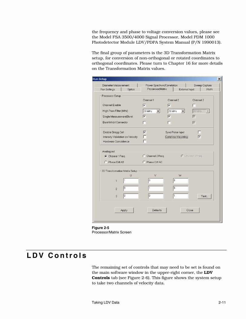
3-2 Optical Setup Page Screen................................................ 3-5 3-3 Processor/Matrix Screen .................................................. 3-6 3-4 Receiver Calibration Screen .............................................. 3-7 3-5 Diameter Measurement Screen......................................... 3-8 3-6 Screen Capture Screen ..................................................... 3-9 3-7 Diameter/Channel 1 Velocity Control Menu ................... 3-11 3-8 Mean Diameter as a Function of PMT Voltage ................. 3-12 3-9 Data Rate as a Function of PMT Voltage ......................... 3-12 3-10 System Graph: Intensity Validation ................................ 3-13 3-11 Diameter Difference Screen Showing Differences
Between Two Independent Measurements of Particle Diameter ........................................................................ 3-14
3-12 Calibration Diode Setup Page After Taking Calibration Data............................................................................... 3-16
3-13 Typical Phase AB, Phase AC Graph After Capturing Calibration Diode Data................................................... 3-17
3-14 Calibration Diode Setup Page After Copying the Mean Phase Values.................................................................. 3-18
4-1 Capture Run Button on the Main Tool Bar ....................... 4-1 4-2 Settings to Utilize Intensity Validation and Probe
Volume Correction ........................................................... 4-2 4-3 Warning Message Pertaining to Auto-Intensity Option ...... 4-3 4-4 Playback Button on the Main Tool Bar ............................. 4-4 4-5 Velocity Statistics ............................................................. 4-5 4-6 Diameter Statistics ........................................................... 4-6 4-7 Measurement Volume Geometry ....................................... 4-7 4-8 Volume Distribution Statistics.......................................... 4-8 4-9 Various Size Distributions .............................................. 4-11 4-10 Diameter Distribution and Fit: Log Normal Screen.......... 4-14 4-11 Volume Distribution and Fit: Rosin Rammler Screen ...... 4-14 4-12 Volume Distribution and Fit: Nukiyama-Tanasawa
Screen with Too Many Bins ............................................ 4-15 4-13 Volume Distribution and Fit: Nukiyama-Tanasawa
Screen going from 0.1 µm/bin to 1.0 µm/bin................. 4-16 5-1 Main Dialog Box for Selecting the Optical Layout.............. 5-2 5-2 Optical Properties of Common Particle Materials .............. 5-2 5-3 Scattering Domains Covering a Wide Range of Relative
Refractive Indices and Off-Axis Angles.............................. 5-3 5-4 Feasible Scattering Modes for Various Domains,
Attenuation Levels and Polarization.................................. 5-5 5-5 Error Message Pertaining to Inconsistent Entries for
Auto Slope........................................................................ 5-7 6-1 Graph Designer Button .................................................... 6-2 6-2 Graph Designer Screen..................................................... 6-3 6-3 Edit Histogram Data Sets Screen...................................... 6-4 6-4 Text Parameters Dialog..................................................... 6-5 6-5 Horizontal Axis Dialog ...................................................... 6-6 6-6 Axis Labels Dialog ............................................................ 6-6

Contents xvii
6-7 Bar Graph Parameters Screen .......................................... 6-7 6-8 Plot Parameters Screen..................................................... 6-8 6-9 Graph Parameters Screen................................................. 6-8 6-10 Diameter Histogram Screen with Information Box ............ 6-9 6-11 Graph Data .................................................................... 6-10 7-1 Statistics Selection Menu.................................................. 7-1 7-2 Velocity Statistics Window ................................................ 7-2 7-3 Diameter Statistics Window.............................................. 7-2 7-4 Volume Distribution Statistics Window............................. 7-3 7-5 Velocity and Size Subrange Statistics Window .................. 7-3 7-6 External Input Subrange Statistics Window...................... 7-4 7-7 Transformed Velocity Statistics Window ........................... 7-4 7-8 Customizing a Statistics Window...................................... 7-5 7-9 Statistics Output Options Window.................................... 7-6 7-10 Statistics Summary Report #1 .......................................... 7-7 7-11 Statistics Summary Report #2 .......................................... 7-8 7-12 Statistics Summary Report #3 .......................................... 7-8 7-13 Statistics Designer Button ................................................ 7-9 7-14 Statistics Designer Screen .............................................. 7-10 7-15 Example Custom Statistics Windows .............................. 7-10 8-1 External Input Screen....................................................... 8-1 9-1 Power Spectrum/Correlation Screen................................. 9-1 9-2 Processor/Matrix Screen .................................................. 9-2 10-1 Subrange Input Menu..................................................... 10-3 10-2 Diameter and Velocity Window for Subrange Example .... 10-4 10-3 FLOWSIZER Window for Lower Velocity Subrange ............. 10-5 10-4 FLOWSIZER Window for Upper Velocity Subrange............. 10-6 10-5 Coincidence Window Setup............................................. 10-8 10-6 Examples of Software Coincidence Checking .................. 10-9 10-7 Software Coincidence Button.......................................... 10-9 10-8 Velocity Bias................................................................. 10-12 11-1 Window for Selecting what Analog Signal to Output........ 11-1 12-1 RMR Screen.................................................................... 12-1 12-2 Automatic RMR Window Generation ............................... 12-5 13-1 Traverse Manager Screen................................................ 13-2 13-2 Communication Setup Dialog Screen.............................. 13-4 13-3 Axis Setup Dialog Screen................................................ 13-5 13-4 Auto Dialog Screen ......................................................... 13-6 13-5 Matrix Dialog Screen ...................................................... 13-8 13-6 Auto Fill-Column Screen................................................. 13-9 14-1 Burst Monitor Window.................................................... 14-2 15-1 Export Data Dialog Box .................................................. 15-1 16-1 Three-Component Velocity Measurement Using Two
Probes in the Same Plane............................................... 16-2

xviii Phase Doppler Particle Analyzer/Laser Doppler Velocimeter (Operations)
16-2 Three-Component Velocity Measurement Using Two Probes not in the Same Plane ......................................... 16-4
16-3 Three-Component Velocity Measurement Using a 5-Beam Probe................................................................. 16-6
16-4 Two-Component Velocity Measurement Using One Probe.............................................................................. 16-7
16-5 Schematic Drawing of Two-Component Near-Wall Velocity Measurement using a Probe with Prism............. 16-8
16-6 3-D Matrix Transformation Setup ................................... 16-9 16-7 3-D Matrix Transformation Test.................................... 16-10 A-1 LDV Technique................................................................. A-1 A-2 Dual-Beam Laser Anemometer ......................................... A-2 A-3 Fringe Descriptions .......................................................... A-4 A-4 Measurement Volume Dimensions ................................... A-5 A-5 Doppler Signal.................................................................. A-6 A-6 Signal Characteristics Along the Measurement Volume .... A-7 A-7 Scattered Light Intensity Variation ................................... A-8 A-8 Typical Frequency versus Velocity Curves ........................ A-9 A-9 Frequency Shifting ......................................................... A-10 A-10 Acousto-Optic (Bragg) Cell.............................................. A-11 A-11 Example Fourier Transforms .......................................... A-15 A-12 Velocity Bias................................................................... A-15
T a b l e s 2-1 Beam Separation Values for TSI Fiberoptic Probes............ 2-7 2-2 Beam Diameter Values for TSI Fiberoptic Probes .............. 2-7
A-1 Sedimentation and Relaxation Time of Unit Density Sphere ........................................................................... A-19

xix
About This Manual
I n t r o d u c t i o n The purpose of this manual is to give step-by-step instructions for proper operation of a LDV or PDPA system. Primary focus of this manual is on the FLOWSIZER
TM software package. Please consult the LDV/PDPA System Installation Manual (P/N 1990024) for step-by-step installation and setup instructions. The TM/TR Series Fiberoptic Probe Manual (P/N 1990021) gives complete instructions on setup, care, and maintenance of your fiberoptic probe. The Model FSA 3500/4000 Signal Processor, Model PDM 1000 Photodetector Module LDV/PDPA System Manual (P/N 1990013) presents a detailed description and specifications of the associated LDV/PDPA electronics.
!
I m p o r t a n t Before turning the FSA on, make sure all connections on the back of the FSA and PDM are secure. All cables should be sufficiently tightened. Failure to secure the connections can damage the PMT voltage supply.
S a f e t y L a b e l s This section acquaints you with the advisory and identification labels on the instrument and used in this manual to reinforce the safety features built into the design of the instrument.
Caution
!
C a u t i o n Caution means be careful. It means if you do not follow the procedures prescribed in this manual you may do something that might result in equipment damage, or you might have to take something apart and start over again. It also indicates that important information about the operation and maintenance of this instrument is included.

xx Phase Doppler Particle Analyzer/Laser Doppler Velocimeter (Operations)
Warning
!
W A R N I N G Warning means that unsafe use of the instrument could result in serious injury to you or cause irrevocable damage to the instrument. Follow the procedures prescribed in this manual to use the instrument safely.
Danger
!
D A N G E R Danger means that unsafe use of the instrument could result in very serious injury or death to you. Follow the procedures prescribed in this manual to use the instrument safely.
Caution, Warning, or Danger Symbols The following symbols may accompany cautions and warnings to indicate the nature and consequences of hazards:
Warns you that uninsulated voltage within the instrument may have sufficient magnitude to cause electric shock and/or death. Therefore, it is dangerous to make any contact with any part inside the instrument.
Warns you that the instrument contains a laser and that important information about its safe operation and maintenance is included. Therefore, you should read the manual carefully to avoid any exposure to hazardous laser radiation.
Warns you that the instrument is susceptible to electro-static dissipation (ESD) and ESD protection procedures should be followed to avoid damage.
Indicates the connector is connected to earth ground and cabinet ground.

About This Manual xxi
G e t t i n g H e l p To report damaged or missing parts, for service information or technical or application questions, contact:
TSI Incorporated 500 Cardigan Road Shoreview, MN 55126 USA Fax: (651) 490-3824 Telephone: 1-800-874-2811 (USA) or (651) 490-2811 E-mail Address: [email protected] Web site: service.tsi.com
S u b m i t t i n g C o m m e n t s TSI values your comments and suggestions on this manual. Please use the comment sheet, on the last page of this manual, to send us your opinion on the manual’s usability, to suggest specific improvements, or to report any technical errors.
If the comment sheet has already been used, mail your comments on another sheet of paper to:
TSI Incorporated 500 Cardigan Road Shoreview, MN 55126 Fax: (651) 490-3824 E-mail: [email protected]


1-1
C H A P T E R 1 Preparing the Computer to Store the Data
I n s t a l l i n g t h e F L O W S I Z E RT M S o f t w a r e
P a c k a g e
If you purchased your LDV/PDPA system computer from TSI, FLOWSIZER
TM software is already installed. If you are supplying your
own computer, FLOWSIZER software must be installed. A Windows® 98SE/2000/XP Professional Operating System is required. The preferred operating system is Windows XP Professional and the preferred amount of RAM is 1GB. Locate the FLOWSIZER CD. Insert it, and if “AutoRun” does not initialize, open it and double-click the Setup.exe icon. Follow the steps in the installation wizard. Connect the FSA processor to the PC and switch the FSA on. Leaving the FLOWSIZER CD in the drive, restart the PC. You may notice a “New Hardware Found” message. If so, Windows is automatically accessing the FLOWSIZER CD and installing the FSA’s FireWire® (IEEE1394) driver. If you do not notice a “New Hardware Found” message, you will need to use the Control Panel’s “Add Hardware” Wizard. If required, browse to the CD drive, then to the FSA.INF file located in the “FSA IEEE-1394 Driver” folder. This will install the FSA’s FireWire (IEEE1394) driver.
C r e a t i n g a N e w S t r u c t u r e f o r D a t a S t o r a g e
The basic storage structure for data taken with FLOWSIZER software consists of a main Project folder that contains various Experiment folders, each of which can contain many runs. Upon installation of FLOWSIZER, a default Project directory entitled TSI Data and a default experiment entitled Default Experiment will be created. There will also be several runs in the default experiment folder,
®Windows is a registered trademark of Microsoft Corporation in the United States and other countries. ®FireWire is a registered trademark of Apple Computer Inc.

1-2 Phase Doppler Particle Analyzer/Laser Doppler Velocimeter (Operations)
which can be “played back” to view some examples of previously collected data. The first step in setting up a place to store your data is to either create a new Project folder or to select an existing one.
To create a new Project folder select File→New Project Directory. A dialog box like the one shown in Figure 1-1 should open.
Figure 1-1 Create Project Directory Dialog Select the target disk drive or folder the new project directory will reside in and click the Create Dir button. A dialog box prompting you to enter a new Project directory name will open. After entering a name for the Project folder click OK.
After creating a new Project directory you must create a new Experiment directory. To do this, select File → Experiment Manager. A dialog box similar to the one shown in Figure 1-2 will open. To create the new Experiment folder select the New Experiment button and then enter a desired name. (The default name will be New Experiment.) The name can be either a word (for example, 10 MPa) or a number (for example, 16). If you would like to use a previous run as a template for all FLOWSIZER software settings, browse to the appropriate Experiment and select (single-click) the Run you would like to clone. Press the Copy button. Then browse back to your new Experiment and press the Paste button. Select (single-click) this Run and press Select.
If you are not selecting a previous Run, after entering the new Experiment name, click the default Run 1 and press the Select

Preparing the Computer to Store the Data 1-3
button. All settings from the most recently saved or opened run will be cloned over to the default Run1 file.
Figure 1-2 Manage Experiments and Runs Screen
Now that both a Project folder and an Experiment folder have been created the final step in setting up the data storage structure is to create a new run. To do this select Run → New Run. A dialog box prompting for a run name will open. Enter a name and hit the OK button. The data file structure is now complete and you are ready to begin taking data.
S e l e c t i n g a n E x i s t i n g P r o j e c t o r E x p e r i m e n t F o l d e r f o r D a t a S t o r a g e
If data is to be stored in a pre-existing Project or Experiment folder, do the following. To select a Project folder go to File → Select Project Directory. A dialog box like the one shown in Figure 1-3 will open. Select the folder name of an existing project and click OK to open.

1-4 Phase Doppler Particle Analyzer/Laser Doppler Velocimeter (Operations)
Figure 1-3 Open Current Project Directory Dialog In order to select an existing Experiment folder, the correct Project folder, which contains the Experiment folder, to be opened must first be chosen. Then select File → Experiment Manager. The dialog box from Figure 1-2 will open. Highlight the Experiment folder that you wish to choose from the left window of the dialog box and hit the Select button. A run from the selected Experiment folder can also be chosen from the list in the right window of the dialog box. If a run is not chosen, a warning dialog box will open. You can ignore it by hitting OK. A run needs to be created before data can be taken in this case.

2-1
C H A P T E R 2 Taking LDV Data
L D V O v e r v i e w Before getting into the details of taking LDV data with your system, a little background on the principle of LDV will be helpful. Laser Doppler Velocimeter measures the velocity of small particles that are moving in the fluid of interest. Assuming the particles are small, the velocity of these particles can be assumed to be the velocity of the fluid itself. The physical principle used to measure the particle velocities is the scattering of light by the particles. The intersection of the two laser beams (for each component of velocity) results in a fringe pattern—a series of light and dark fringes. As a particle moves through the measuring volume, it scatters light when it crosses a bright fringe, and scatters no light as it passes a dark fringe. This results in a fluctuating pattern of scattered light intensity with a frequency proportional to the particle velocity. Since the distance between fringes and the time for the particle to go from one fringe to the next (inverse of signal frequency) are known, the measured signal frequency can be converted to velocity. The scattered light is collected by optics and converted to electrical signals by Photomultiplier Tubes (PMTs). The frequency of the
signal (also known as Doppler frequency Df ) is measured and then
the velocity u is calculated by multiplying the frequency by the
fringe spacing fδ , i.e.
Df fu δ= .
If the two laser beams that interfere are of exactly the same frequency, the fringes will be stationary in the measuring volume. One problem with this is that particles with a certain velocity moving one way across the fringes may have exactly the same frequency as particles (having the same magnitude of velocity) moving in the opposite direction. Thus there would be no way to determine if particles were moving in a positive or negative flow direction. To eliminate this problem in LDV systems, one of the two laser beams is frequency shifted by a Bragg cell by 40 MHz. This results in fringes that are essentially moving at a rate of 40 MHz in the measuring volume. Particles crossing the measurement volume will now have a frequency either above or below 40 MHz, depending on their direction. Thus the frequency of light scattered by a

2-2 Phase Doppler Particle Analyzer/Laser Doppler Velocimeter (Operations)
particle will be 40 MHz plus or minus an amount due to its velocity. If a particle is moving against the fringes, it will have a frequency of 40 MHz plus the Doppler frequency (the frequency due to the particle velocity) and if a particle is moving with the fringes it will have a frequency of 40 MHz minus the Doppler frequency. Frequency shifting also allows you to measure velocities near zero, where without the shifting there would be no oscillating pattern of light scattered from the particle at all. Another factor in the light scattering pattern is due to the Gaussian nature of the intensity laser beams. This results in bright fringes that have more intensity as you move towards the center of the ellipsoidal measuring volume. Thus a particle crossing through the measuring volume will result in a light scattering pattern similar to the one shown in Figure 2-1.
Time Figure 2-1 Light Scattered by a Particle Passing Through the LDV Measurement Volume The scattered light is collected and transmitted to the PMTs through optical fibers. The PMTs generate electrical signals representing the incoming optical signals. The output of the PMT is first high-pass filtered to remove the low frequency portion of the signal due to the Gaussian beams. This low frequency envelope is called the pedestal. After removing the pedestal, the signal (consisting of the 40 MHz ± the Doppler shift) is mixed with another signal whose frequency can range from 0−40 MHz. The difference (low frequency portion of the mixed signal) signal is then passed through to a selectable series of bandpass filters. This process of mixing is often called downmixing. It allows you to select the optimum frequency shift to resolve reversing and zero flow situations. In cases where the flow is not reversing, downmixing by 40 MHz may be appropriate as it essentially removes the 40 MHz that was added by frequency shifting. After downmixing, the signals are passed through a user selectable series of bandpass filters. Passing the signals through the bandpass filters helps improve the Signal to Noise Ratio (SNR) of the signals by eliminating noise. The signal frequencies are then measured using the signal processor.

Taking LDV Data 2-3
Note: The following procedure will set up the system for general-purpose data collection, but may not be exactly appropriate for specific applications.
D i r e c t i o n o f F r i n g e M o t i o n R e l a t i v e t o P a r t i c l e M o t i o n f o r V e l o c i t y M e a s u r e m e n t s
The positive velocity direction for a given velocity component will be such that the particles cross the measurement volume against the motion of the fringes. To determine what direction the fringes are moving in the measuring volume, consider looking at the measuring volume from the vantage point of the transmitter. Determine which beam is the shifted beam and which is the unshifted for a particular pair of beams. (To do this, look on the fiberlight and close the shutter on either the shifted or unshifted beam, and see which one shuts off.) The fringe motion will be from the shifted to the unshifted beam.
R u n S e t u p → R u n S e t t i n g s After setting up and connecting the hardware and creating or selecting a Run to store your data the following will provide an overview of how to take data with the system. The first set of software settings to be checked is found by selecting Run → Run Setup. Then choose the Run Settings tab. A dialog box similar to the one shown in Figure 2-2 should now be open. The following parameters need to be selected.
1. Maximum Particle Measurement Attempts—This is the maximum total number of particle attempts to take in a run. This refers to the number of valid bursts detected, and not to the number of velocity or diameter measurements obtained from those bursts. In random (verified) mode, data acquisition will stop when the total samples from all active channels reaches this value. In hardware coincidence mode, data acquisition will stop when this number of samples is acquired from each channel enabled. In software coincidence mode, data acquisition will stop when this number of samples is acquired from each enabled channel. However, playback with different coincidence gate scale and/or coincidence interval settings will yield a different number of total samples captures. The reason for this is that with software coincidence, all samples are collected and saved—the non-coincident ones are simply not displayed or allowed to enter any statistics.

2-4 Phase Doppler Particle Analyzer/Laser Doppler Velocimeter (Operations)
Figure 2-2 Run Settings Screen
2. Screen Update Intervals—The screen update size sets how often the screen is updated. During data acquisition, a value of zero shuts off this feature. A Screen Update Interval value of 1000 means the screen is updated after 1000 particle attempts are completed. It is suggested to use 0, which means the software will determine the screen update speed. This is especially useful in Capture Run, which captures data directly.
3. Time Out—This value is the length of time the run will stay open with no data being detected. A value of 0 means the run will not stop due to a data rate of zero.
4. Enable Software Slave Mode—By selecting this option an external computer could be used to control the data-taking computer. The control can be done through RS 232.
5. Enable Auto Export—This option instructs the FLOWSIZER software to automatically do an ASCII Export of currently selected ASCII export values, each time a run is captured and saved.

Taking LDV Data 2-5
Hints, Suggestions, and Comments
1. The Maximum Particle Measurement Attempts will be limited by the amount of memory that your computer contains. The recommended amount of memory is currently 1GB.
2. Unless there is a specific reason, set the Screen Update Interval, Maximum Run Time, and Time Out to 0. This means that your run will only stop due to the maximum number of particle measurement attempts.
3. With a highly varying data rate, such as from a pulsed spray device, setting a Screen Update Interval of 0 may result in data overflow. It is suggested that Screen Update Interval values of 1000 to 5000 be used to prevent this.
4. When collecting data from a high data rate flow, there is a possibility that the system will get a data overflow error, which will prematurely stop the run. To improve performance in this case, set the Screen Update Interval to a large value, or if even this is unsuccessful, try capturing data with the Quick Capture mode (<F8> or the button on the Main Menu box). In this mode, the system will capture data without updating the screen at all. After capture is complete, the data can then be saved and replayed without having any data overflow problems.

2-6 Phase Doppler Particle Analyzer/Laser Doppler Velocimeter (Operations)
R u n S e t u p → O p t i c s After selecting values for the Run Settings tab, click the Optics tab from the same dialog box. The dialog box should now look like the one shown in Figure 2-3.
Figure 2-3 Optical Setup Page Screen
The following parameters need to be set correctly in order to take accurate velocity data.
1. Wavelength—Wavelength of the laser light for each channel (velocity component). This is laser dependent and should not be modified unless the laser is changed. Argon Ion laser wavelengths are 514.5 mm (green), 488.0 nm (blue), and 476.5 nm (violet).
2. Focal Length—Focal length of the front lens in the fiberoptic transmitter or transceiver probe usually found on the case of the lens. This parameter must be updated if the lens is changed.

Taking LDV Data 2-7
3. Beam Separation—Distance between the two laser beams of one color from the probe, measured prior to the beam expander and the transmitter lens. See the table below for the correct value to use for your probe. If a beam expander is present, do not change the value—the software will account for the effect of the beam expander through the Beam Expander ratio.
Table 2-1 Beam Separation Values for TSI Fiberoptic Probes
Probe Series Beam Separation
TR 10 Series 15 mm Diameter
7.5 mm
TR 20 Series 25 mm Diameter
15 mm
TM 50 Series 70 mm Diameter
20 mm
TR 60 Series 83 mm Diameter
50 mm
TR 360 Series 5 Beam Probe
25 mm (Green, Violet) 50 mm (Blue)
4. Laser Beam Diam—Gaussian diameter of the laser beam before the focusing lens and before the beam expander, if any. See the table below for the correct value to use for your probe. If a beam expander is present, do not change the value—the software will account for the effect of the beam expander through the Beam Expander ratio.
Table 2-2 Beam Diameter Values for TSI Fiberoptic Probes
Probe Series Beam Diameter
TR 10 Series 15 mm Diameter
0.5 mm
TR 20 Series 25 mm Diameter
1.0 mm
TM 50 Series 70 mm Diameter
1.77 mm
TR 60 Series 83 mm Diameter
2.65 mm
TR 360 Series 5 Beam Probe
1.8 mm (All Beams)
5. Beam Expander—Expansion or contraction ratio of a beam expander or contractor. If an expander or contractor is not present, this field is set to 1. The Model XPD50-I has an expansion ratio of 2.00 when installed as a beam expander, and an expansion ratio of 0.50 when installed as a beam contractor. The Model XPD60 has a fixed expansion ratio of 2.60. If a beam expander is present, do not change the Laser Beam Diam or

2-8 Phase Doppler Particle Analyzer/Laser Doppler Velocimeter (Operations)
Beam Separation values—the software will account for the differences in these values through the Beam Expander ratio.
6. Fringe Spacing—Spacing between fringes in the measurement volume, dependent on other parameters. The fringe spacing (δf) is:
( )κλδ
sin2f =
λ = wavelength of laser 2κ = angle between beams The Fringe Spacing will be automatically calculated by the software based on the previously entered optical parameters. You can also manually select the Fringe Spacing by clicking the “...” button (next to the computed fringe spacing value), checking the Manual Input checkbox, and then entering a value for the fringe spacing.
Note: Once the “Manual Input” checkbox is enabled, future runs created from this run will also have this checkbox enabled. Remember this if optics are subsequently changed, you will again need to manually update the fringe spacing.
7. Bragg Cell Freq—Amount of optical frequency shifting. For typical operation with fringe motion against the positive direction, this value is set to 40 MHz. For special operation with fringe motion in the positive direction, this value is set to -40 MHz.
8. The Diameter Min and Diameter Max limits are the theoretical measurement limits calculated by the system, with the standard assumption of a linear phase to diameter relationship. Uncheck the Enforce checkbox to disable adherence to these limits. Be aware that the smallest diameter droplets will have lower measurement reliability if this is done.
9. Enforce—Enforce the diameter units so diameters measured outside the range will be ignored.
R u n S e t u p → P r o c e s s o r / M a t r i x After setting the parameters from the Optics tab, click the Processor/Matrix tab from the same dialog box. The dialog box should now look like the one shown in Figure 2-5.
Check to see that the following parameters are set correctly:
1. Channel Enable—Enable the correct number of channels by checking or unchecking each box. Though not necessary, it is good practice to disable channels not currently being used.

Taking LDV Data 2-9
2. High-Pass Filter—Selects the high-pass filter which removes the signal pedestal (due to the Gaussian laser beams) from the Doppler signal. For most applications, choose 20 MHz. This filtering is performed on the signal in the PDM before downmixing. Use the 5 MHz filter for high velocity reversing flows because the raw PMT signal can drop below 20 MHz and be attenuated. Use the 20 MHz filter for very short transit time signals because the 5 MHz may not remove the entire pedestal.
3. Single Measurement/Burst—For almost all applications, enable this check box. This will allow the processor to only take one valid measurement per particle, no matter the length of its gate time. Disable the check box only to arbitrarily break up continuous sinewave type signals into multiple bursts.
4. Burst Inhibit Connector—Data collection for each channel can be inhibited using the burst inhibit connector on the back of the FSA. Bursts are inhibited when a logic high (+5V) is applied to this connector. These check boxes control which channels are affected by the signal at the connector. For example, checking the channel 2 box, but not the channel 1 and 3 boxes, would cause only channel 2 to be inhibited when a logic high is applied at the connector. When the connector is driven low, or nothing is connected to it, these boxes have no effect because nothing is being inhibited. See also the FSA hardware manual.
5. Enable Bragg Cell—Checking this box enables the 40 MHz signal from the FSA to the fiberlight. It must be checked during normal operation. It would only be unchecked during some debugging situations to disable the shifted beams.
Items 6 through 9 are not selected in the example shown (Figure 2-5)
6. Enable Sync Pulse Input—Check this box if you are using the sync pulse BNC connector on the back of the FSA. A rising logic level (+5V) applied to this connector will reset the time stamp during data collection (see FSA hardware manual). If this is being done, this box must be checked so the FLOWSIZER
software knows the time stamp will be resetting.
7. Enable Intensity Validation on Velocity—Intensity validation is normally only used with phase Doppler systems. The height (or intensity) of the pedestal of each channel 1A particle is measured and compared to its size calculated by the phase Doppler method. This box does not have to be checked for phase Doppler measurements. However, intensity measurements can also be used with velocity (LDV) measurements, but only if you have a phase Doppler system, or if you ordered the intensity board as a special option. The intensity board is in the PDM and measures the pedestal

2-10 Phase Doppler Particle Analyzer/Laser Doppler Velocimeter (Operations)
heights of channel 1A only. To use the intensity information with velocity data only, check this box. Select the range of intensities you wish to accept/exclude under the Subrange (Under/Over) tab, minimum and maximum intensity. Then enable this subranging by selecting Software Subrange and Software Coincidence.
8. Enable Gatetime Weighting—Check this if you need to get velocity-bias corrected statistics. Gate time (transit time) is used as the weighting function. Velocity bias is caused by the fact that more of the faster particles go through the measuring volume per second. Therefore, the sampling of velocity is not representative of the true flow, but is biased with the faster ones. This causes the measured velocity mean to be higher than the actual, especially with a broad velocity distribution. Checking this box causes each velocity data point to be normalized or weighted with its own gate time. Slower particles have longer gate times and, therefore, more weight. With this weighting, the calculated mean velocity is closer to the actual mean. An even better method to remove velocity bias is to use even-time sampling, see Chapter 10 for more details.
9. Hardware Coincidence—Check this if you wish to enable hardware coincidence. This will require overlap of burst gates of active channels, in order for the data to be considered coincident. Note that hardware coincidence is only applicable to 2 and 3 channel systems. Non-Coincident data is discarded, which reduces file storage size, but remember that unlike software coincidence, there is no way to recover non-coincident data at a later time. Refer to Chapter 10 for more details on software coincidence. When Hardware Coincidence is enabled, the Coincidence Data Rate will be enabled on the Hardware Status Screen (see Figure 2-4).
Figure 2-4 Hardware Status Screen The next group of parameters allows selection of the value to send out the FSA processor Analog Out connector. This is a 0 to 10V signal, updated for every burst in the selected channel. The signal will remain at 0.0V until the first valid sample arrives. The user may connect a load up to 30mA on this line. For more details on
Taking LDV Data 2-11
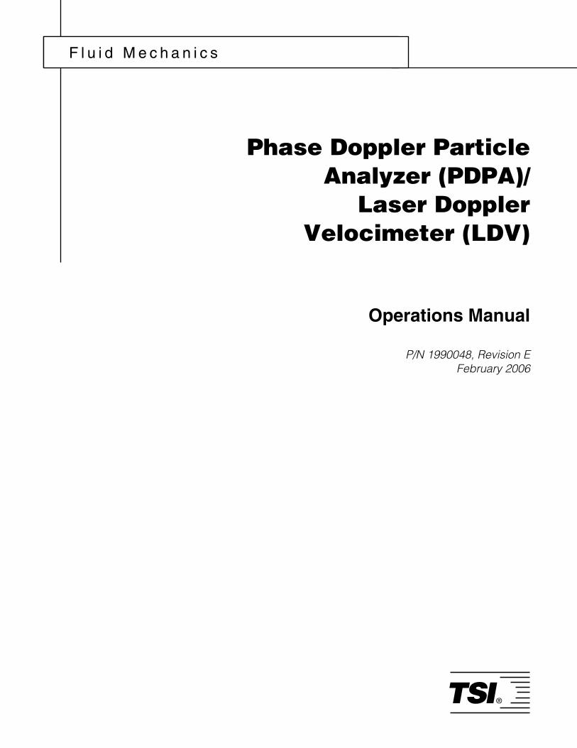
the frequency and phase to voltage conversion values, please see the Model FSA 3500/4000 Signal Processor, Model PDM 1000 Photodetector Module LDV/PDPA System Manual (P/N 1990013). The final group of parameters is the 3D Transformation Matrix setup, for conversion of non-orthogonal or rotated coordinates to orthogonal coordinates. Please turn to Chapter 16 for more details on the Transformation Matrix values.
Figure 2-5 Processor/Matrix Screen
L D V C o n t r o l s The remaining set of controls that may need to be set is found on the main software window in the upper-right corner, the LDV Controls tab (see Figure 2-6). This figure shows the system setup to take two channels of velocity data.

2-12 Phase Doppler Particle Analyzer/Laser Doppler Velocimeter (Operations)
Figure 2-6 LDV Controls Menu The selection of the parameters on the LDV Controls Menu is probably the most important for getting good velocity measurements. The process is often times slightly iterative among the various parameters. Following is a general procedure that will help you acquire good data in many applications. Keep in mind you will have to select parameters independently for each channel of velocity, you wish to measure.
D o w n m i x i n g The fiberlight’s Bragg cell adds 40 MHz to the shifted beams, which causes the fringes for each color to move at 40 MHz. This causes 40 MHz to be added to the Doppler frequency of each burst. A particle, or solid surface, sitting stationary in the measuring volume will generate a 40 MHz signal. This allows flow reversals to be determined and also enables a range of frequencies to be compressed into a 1:10 range. Some or all of this 40 MHz can be removed by the downmixing done in the FSA. Dowmixing subtracts

Taking LDV Data 2-13
the downmix frequency from the input signal. The downmix frequency is entered in the Downmix Freq. (MHZ) box. Entering 40 MHz will eliminate all the 40 MHz Bragg Cell Shift, so only the Doppler frequency is left, which is proportional only to the particle velocity. Entering 39 means 39 MHz is subtracted from the 40 MHz Bragg cell shift, leaving 1 MHz still added onto the Doppler frequency. This will allow flow reversals up to 1 MHz to be measured. With a 5 µm fringe spacing, this would correspond to flow reversals up to 5 m/s. Entering 36 means 36 MHz is subtracted from the 40 MHz Bragg cell shift, leaving 4 MHz still added onto the Doppler frequency. This would correspond to 20 m/s (assuming 5 µm fringe spacing), in terms of the maximum flow reversal velocity. Entering 0 means dowmixing is bypassed so the entire 40 MHz is still left on the signal. When your Doppler frequency is 20 MHz or lower, you should always use downmixing. This allows you to use the narrowest bandpass filter range on the signal after downmixing to remove the most possible noise. A common starting point is to use a 36 MHz downmix frequency, and the 1–10 MHz bandpass filter setting. When the Doppler frequency is above 40 MHz you should bypass dowmixing. This is because downmixing produces two frequency components, the sum and difference between the input signal and the downmix frequency. The bandpass filters remove the sum term, leaving the difference term, which is what we want. When the difference term is near or above 40 MHz, the sum term cannot be fully filtered out resulting in a distorted signal that may give erroneous frequency readings. A Doppler frequency which is between 20 and 40 MHz is in a transition region where downmixing or bypassing downmixing both may work. For this reason, signals being downmixed pass through an 80 MHz low-pass filter. This prevents downmixing from being used for Doppler frequencies over 40 MHz. When downmixing is bypassed, this 80 MHz low-pass filter is also bypassed. Leaving some or all of the 40 MHz on the signal is necessary when your flow is going both directions through the measuring volume. This way the flow direction can be determined, and the FLOWSIZER software then calculates the actual velocity since it knows the amount of frequency that was left on. Even without reversing flows, if your range of Doppler frequencies doesn’t fit within one of the bandpass filter ranges, you must downmix by less than 40 and leave some shift on the signals. A third reason for leaving some shift on is if some particles are traveling nearly parallel to the fringes in the measuring volume. In this case they wouldn’t cross many fringes and not generate enough frequency cycles to be detectable by the processor. Leaving shift on adds cycles to each

2-14 Phase Doppler Particle Analyzer/Laser Doppler Velocimeter (Operations)
burst, making them easily distinguishable from noise. Other than for these reasons, you should generally not leave shift on because adding many cycles to a burst begins to put it out of the region where the processor was optimized, i.e., short bursts in the neighborhood of 5–50 cycles each.
B a n d P a s s F i l t e r Normally the first parameter to select is the Band Pass Filter setting. If you know the range of frequencies that will be in the flow, you can select the setting directly. Remember that the signal frequency (without frequency shift) is equal to the particle velocity divided by the fringe spacing. To estimate the frequency of the signal input to the signal processor, add the effective frequency shift (equal to 40 MHz minus the downmix frequency). If you are unsure, select the 1–10 MHz setting (also use a PMT Voltage of 400, a Burst Threshold of 30, an SNR of medium, and a Downmix Freq. of 36). Then check the Data Rate found on the Hardware Status portion of the main software page. If the data rate is zero, try a different filter range until a non-zero data rate is detected. At this point, you can view the data by capturing in real-time mode. To do this, go to Run → Real Time View (or hit <F6>). Before capturing data you want to have the Frequency Histogram graph open for the channel that you are working with (e.g., use Graphs → Frequency1 Histogram for data on Channel 1). (See Chapter 6, “Using and Creating Graphs,” if you are unsure of how to do this.) As data is being updated to the screen, you should see a frequency histogram appearing. You will know whether or not you have the correct bandpass filter selected depending on how the histogram looks. If the histogram count drops close to zero on both ends of the distribution within the selected bandpass filter range, you can be confident you have selected the correct filter range. Figure 2-7 is an example of a run with the correct bandpass filter selection. Figure 2-8, on the other hand, is an example of an incorrectly chosen bandpass filter range. Notice how the distribution is clipped on the upper end of the frequency distribution. In this example you should change the bandpass range to 2–20 MHz. If a distribution has a frequency range that does not fit within any of the bandpass filter ranges (for example, a frequency distribution ranging from 500 kHz to 4 MHz), you may need to increase the frequency shift (or decrease the downmix frequency) value to make the frequency distribution fit within one of the bandpass ranges. To do this you change the Downmix Freq. to a smaller number. The frequencies of your signals will then be increased by whatever the difference is between the number you select and 40 MHz. For example, changing

Taking LDV Data 2-15
the Downmix Freq. to 39 MHz will increase all the frequencies by 1 MHz (40–39=1 MHz). In the example given previously (a frequency distribution ranging from 500 kHz to 4 MHz), changing the Downmix Freq. to 39 MHz will result in a frequency distribution ranging from 1.5 MHz to 5 MHz. The distribution will now fit in the 1–10 MHz bandpass filter range.
Frequency 1 Histogram
1.8 3.6 5.4 7.2 9.0 10.8 12.6 14.40
2000
4000
6000
8000
10000
Frequency Ch. 1 (MHz)
Freq
uenc
y C
ount
Ch.
1
Figure 2-7 Example of a Good Frequency Histogram Taken with a Bandpass Filter Range of 1–10 MHz

2-16 Phase Doppler Particle Analyzer/Laser Doppler Velocimeter (Operations)
Frequency 1 Histogram
2 4 6 8 10 12 140
1200
2400
3600
4800
6000
Frequency Ch. 1 (MHz)
Freq
uenc
y C
ount
Ch.
1
Figure 2-8 Example of a Cut-Off Frequency Histogram Taken with a Bandpass Filter Range of 1–10 MHz
After the correct Band-Pass Filter range has been selected you will want to optimize the PMT Voltage, Burst Threshold, and SNR parameters for your specific application. A discussion of important considerations follows:
P M T V o l t a g e This parameter sets the voltage that is applied to the PMT for each channel. Increasing the voltage increases the gain of the PMT in a roughly linear fashion. This increase in gain applies not only to the signal, but also to any associated noise. In order to choose an optimum voltage, the following considerations are important. As the voltage is increased, signals from smaller particles (which scatter less light) will be gained up enough to be detected by the processor. Thus increasing the voltage should in general increase the data rate. At a certain point, however, increasing the voltage will not provide much benefit and may actually reduce the data rate. Since the signal will generally have larger amplitude than noise, and since the electronics begin clipping a signal at a certain point, increasing the voltage beyond a certain point will simply reduce the SNR. For many applications, the optimum voltage range will fall between 350 V and 600 V.

Taking LDV Data 2-17
B u r s t T h r e s h o l d The Burst Threshold is another very important variable in taking LDV data. Often times, the best way to optimize your data is to iterate between adjusting the PMT Voltage and the Burst Threshold. The Burst Threshold is the analog voltage level that a signal must reach before the burst gate in the processor will open. (Note: Burst Threshold is only one of the two requirements for opening the burst gate. The other requirement is a certain SNR-level based on a real-time Fourier transform). In general larger particles scatter more light and thus will have higher signal amplitudes. Also, increasing the PMT Voltage will increase the signal amplitudes, which is why the Burst Threshold level cannot be adjusted without considering the PMT Voltage. Typical Burst Threshold values will range from 30 mV to 300 mV. For applications with small particles (<10 µm) the optimum will probably be 30 mV or slightly higher than that. On the other hand, with large particles an optimized value might be 100 mV or 200 mV. In situations with high background light levels, such as near wall measurements or measurements in a dense medium, Burst thresholds over 500 mV may be needed to achieve the best data rate. The signal out BNC connector on the FSA front panel shows the signal as it is when it passes the burst threshold circuit. When the connector is attached to an oscilloscope 50 ohm input, the amplitude seen on the scope matches the burst threshold in millivolts. For example, if the burst threshold is set to 100 mV, a burst signal showing an amplitude of ±100 mV on the scope is just at the threshold.
S N R The SNR (signal-to-noise ratio) sets the validation threshold used by the FSA’s burst validation subsystem, when evaluating bursts passed on from the burst detector. An SNR of “High” means only the best quality bursts pass validation. This results in more accurate frequency and phase data, but also a lower data rate. An SNR setting of “Very Low” means noisier bursts are validated, resulting in higher data rates. These noisier bursts still represent valid flow or size data, but just not as accurately. The SNR setting has no effect on the FSA’s burst detector, but only on its burst processing validation. Because of this, choosing a higher SNR level will result in a decrease in the burst efficiency. The selection of SNR also sets a minimum number of cycles required for a burst to be

2-18 Phase Doppler Particle Analyzer/Laser Doppler Velocimeter (Operations)
validated. Thus you would use an SNR setting of “Very Low” when measuring bursts with just a few cycles or to measure bursts of very short transit time.
H a r d w a r e S t a t u s The hardware status window is in the lower right-hand corner of the screen. The Data Rate (Hz) is the number of bursts passing validation per second for each channel. In phase Doppler systems, channel 1 indicates the phase data rate. This data rate reflects the processor output and is unaffected by software settings such as subranging, coincidence, or even-time sampling. Burst Eff (%) is percent burst efficiency. It is the ratio of burst detector triggers to valid bursts. For example, the burst detector puts out 10,000 bursts per second, each one having one burst gate and 2,500 per second were considered valid after burst processing. The data rate would be 2,500 and burst efficiency 25%. Poor SNR signals will have lower burst efficiencies.
PMT Volt Sat. will light up if the PMTs are saturated from getting too much light. These indicators mirror exactly the lights on the PDM front panel. When saturation is indicated, the PMT voltage is clamped to some value lower than that requested. During saturation only, this actual PMT voltage is shown under Sat. Volt. (V). Note that the channel 1A, 1B, 1C PMTs share one common high voltage supply, but may not match in saturation because of different light levels to each PMT. When one of the three saturates, it clamps the high voltage for all three. FSA Connection shows whether the FSA has established a communication link to the computer. It also shows the FSA model, 4000 or 3500. Connection will be automatically established when the FSA is powered on and the FireWire cable is connected between the FSA and computer. Coincidence Data Rate displays the hardware coincidence data rate when it is enabled.

3-1
C H A P T E R 3 Taking Size and Velocity Data
Note: This section assumes that the system hardware is set up correctly, i.e., an optical layout has been chosen for sizing (see Chapter 5, “Selecting An Optical Layout for Particle Sizing”). You should also already be familiar with operating the system to take velocity data. The following procedure will help optimize the system for general applications. Difficult applications may require changes from the standard procedure and nothing can substitute for experience in using the system.
P h a s e D o p p l e r O v e r v i e w Before going into the details of taking size data, a brief overview of the phase Doppler (sizing) technique will be given. Phase Doppler measurements allow for the sizing of spherical particles (typically liquid sprays, but also some bubbles and solid spheres). Along with size information, the velocity of the particle is also obtained, so in this sense the phase Doppler technique is an extension of LDV. The size of particles that can be measured is limited, at the low end by the amount of light (which depends on particle size, laser power, and light collecting optics) that is scattered by very small particles, and is limited at the high end by the Gaussian nature of the laser beams (and the far field condition). Typical limits for common configurations might be 1 or 2 μm on the lower end and 500 μm to 1 mm on the upper end. To explain the physical principle used to measure the size of particles, the explanation of the measuring volume consisting of a series of moving fringes will again be used. As a particle moves through the measuring volume, it “scatters these fringes” all around, including some towards the optical receiver. The frequency of the scattered light determines the velocity of the particle. Only one detector is required to get this temporal frequency of the scattered light. However, the spatial frequency (spacing between the scattered fringes at the light collecting optics) of the scattered fringes contains information about the size of the particle being

3-2 Phase Doppler Particle Analyzer/Laser Doppler Velocimeter (Operations)
measured. In order to measure this spatial frequency a minimum of two detectors is required. The spatial frequency is measured as a phase shift between the two electrical signals resulting from the scattered light. This phase shift can then be related to particle size provided the correct optical layout is used. In TSI phase Doppler systems, three separate detectors are used. Thus, two independent measurements of size are obtained. This allows for redundancy in measuring size as well as an improved dynamic size range with high sensitivity. One problem with measuring size (phase difference or phase shift) is to ensure that the phase shift measured by the processing electronics is only “caused” by the particle. Because electronic circuitry can introduce its own phase shifts between two signals, it is often necessary to calibrate away the shift introduced by the electronics. This is done by measuring the phase shift from a light source with a known phase difference. Any deviation from the expected phase shift is then due to the electronics and can be calibrated away. In TSI systems a red laser diode is used as the calibration light source. By splitting the diode light into three parts we can be sure there is no phase shift in the optical signals themselves. Thus any measured phase shift must be due to electronics. Another important sizing feature that TSI systems provide is a measurement of the scattered light intensity for each particle. Intensity measurement is useful because it helps eliminate erroneous size measurements and also provides a better characterization of the measuring volume size, which is useful in calculating certain flow properties.
D i r e c t i o n o f F r i n g e M o t i o n R e l a t i v e t o R e c e i v e r O r i e n t a t i o n f o r S i z i n g M e a s u r e m e n t s
(For more information, see “Direction of Fringe Motion Relative to Particle Motion for Velocity Measurements” in Chapter 2.) When taking size data, it is critical that the PDPA receiver be oriented properly with respect to the direction of the fringe motion. When looking in the PDPA receiver eyepiece, the arrow you see should be pointing in the positive velocity direction when you are using refraction or internal reflection lightscatter modes. This means that the fringe motion will be upward when the arrow in the

Taking Size and Velocity Data 3-3
receiver is pointing down (upward and downward being with respect to gravity, i.e., the usual understanding of up and down). If you are collecting light that is due to reflection off of the particles, the receiver must be rotated 180 degrees. In this case, the fringe motion and the arrow in the receiver will be in the same direction. For the special case of inverting the transmitter/transceiver probe to “subtract” 40 MHz from high-speed flows, the above rules hold. For example, with refraction or internal reflection, the receiver arrow will still point in the positive flow direction. Remember to enter “–40MHz” as the Bragg cell frequency in the optics setup page. See “Run Setup → Optics”in Chapter 2 for details.
S e t t i n g U p t h e S o f t w a r e The following will go through the operation of the software required to take size data. Many of the same screens that were set up for taking velocity data will have to be set for taking size data. The first thing to do is to make sure you have an appropriate file structure (project, experiment, and run) to save data to. See the Chapter 1, “Preparing the Computer to Store Data,” for more details if you are unclear on how to do this. The first screen to set up is found under Run → Run Setup. Then select the Run Settings tab, as shown in Figure 3-1. Explanations of how to set up this screen are found in Chapter 2, “Taking Velocity Data.”

3-4 Phase Doppler Particle Analyzer/Laser Doppler Velocimeter (Operations)
Figure 3-1 Run Settings Screen
R u n S e t u p → O p t i c s The second screen to set up is the Optics tab that is also found under Run → Run Setup (Figure 3-2). Most of the setup explanations found on this screen are also found in Chapter 2, “Taking LDV Data.” However, a few additional comments are in order:
1. Diameter Limit Min—The smallest measurable particle size with the current optical setup. This value will depend on the transmitter fringe spacing, the PDPA receiver focal length, and the “slope,” which is calculated on the Run → Run Setup, Diameter Measurement tab.
2. Diameter Limit Max—The largest measurable particle size with the current optical setup. Depends on the same parameters as the Diameter Limit Min.

Taking Size and Velocity Data 3-5
Figure 3-2 Optical Setup Page Screen 3. RCV Front Lens f.l.—The focal length of the front lens in the
PDPA receiver.
Note: This value is not altered when performing underwater measurements.
4. RCV Back Lens f.l.—The focal length of the internal lens in the PDPA receiver. This value should always be set to 250 mm for RV 70 series receivers and 370 mm for RV 100 series receivers.
5. Slit Aperture—The width of the slit in the PDPA receiver. The slit width affects the size of the measuring volume in which particles will be detected. It is important to have this parameter correct when measuring number density or volume flux. The slit width can be read through the eyepiece in the PDPA receiver, and the standard value is 150 µm. Optional slits are available from TSI with widths of 25 µm and 50 µm for better measurement of dense flows.

3-6 Phase Doppler Particle Analyzer/Laser Doppler Velocimeter (Operations)
After finishing the setup of the Optics page you will need to set up the Processor/Matrix tab (Figure 3-3). You must have at least Channel 1 enabled to take size data. See Chapter 2, “Taking Velocity Data,” for more discussion of the parameters on this screen. Note: The positive direction of any velocity component is given by the
direction that goes from the unshifted beam to the shifted beam, at the transmitting lens. Using this, you can set up the transmitting probe(s) to have the proper coordinate system.
Figure 3-3 Processor/Matrix Screen
Taking Size and Velocity Data 3-7
R u n S e t u p → C a l i b r a t i o n The next screen to setup is found by clicking Run → Calibration, and then selecting the Receiver Calibration tab (Figure 3-4). You should verify that the Detector Separation values for AB and AC are entered correctly. Each PDPA receiver has slightly different values that are determined at TSI prior to delivering the system. The values should be found on your receiver.
Figure 3-4 Receiver Calibration Screen

3-8 Phase Doppler Particle Analyzer/Laser Doppler Velocimeter (Operations)
R u n S e t u p → D i a m e t e r M e a s u r e m e n t The next screen is reached through Run → Run Setup, Diameter Measurement tab (Figure 3-5).
Figure 3-5 Diameter Measurement Screen To enable particle sizing you should enable both the AB enable and the AC enable check boxes. Enabling both boxes will provide the two independent size measurements that will provide the most accurate data. It is possible to enable only one of the boxes, but this is not a normal mode of operation. The mode of checking only AB or AC is used if you only have two input signals into the FSA. The Particle Properties portion of the screen also needs to be set up correctly. The correct selection of these parameters is covered in Chapter 5, “Selecting an Optical Layout for Particle Sizing.”

Taking Size and Velocity Data 3-9
R u n S e t u p → S w e e p C a p t u r e The next screen is reached through Run → Run Setup, Sweep Capture tab (Figure 3-6).
Figure 3-6 Sweep Capture Screen
Sweep Capture is used to record data while the traverse is in motion. This method of data collection is used to rapidly acquire data across an entire spray plume. Keep in mind that the final averaged values are number-density (concentration) weighted.
You must have traverse hardware installed to use this feature. The traverse movement is limited to one axis.

3-10 Phase Doppler Particle Analyzer/Laser Doppler Velocimeter (Operations)
When a Sweep Capture Starts:
If the Traverse Manager is not active it will be activated.
The Traverse is moved to the starting position.
The recording of data begins.
The Traverse is moved along the selected axis.
When the end position is reached the traverse stops and data collection ends.
D i a m e t e r M e a s u r e m e n t Now go to the Diameter Measurement tab (Figure 3-7) found in the upper right corner of the main software window. If you are using more than one channel of velocity you will control channels 2 and/or 3 from the LDV Controls tab. Since size data is taken on channel 1, you will control the channel 1 velocity from the Diameter Measurement tab. Many of the same considerations are important to choosing these parameters as when taking velocity data, so reviewing the LDV Controls tab explanations in Chapter 2 would be very helpful at this point. Remember, you must select the bandpass filter range so that you aren’t cutting off any frequencies that may correspond to particle velocities in the flow. The PMT voltage setting for sizing is more critical than for velocity because it affects the measurable size range of the instrument. The voltage must be large enough to detect the smaller particles in the flow, yet low enough so that excessive PMT saturation does not occur. Particles scatter light in proportion to the diameter squared (d2).

Taking Size and Velocity Data 3-11
Figure 3-7 Diameter/Channel 1 Velocity Control Menu In order to set the voltage level for taking size data, the following procedure is recommended. With the system taking data, observe the D10 (diameter mean). Increase the PMT voltage until the value of the diameter mean is stable with PMT voltage. As you increase the voltage, the smaller particles will become measurable. When the voltage is large enough, most of the smaller particles will be detected, and the D10 will stabilize. Figure 3-8 illustrates the relationship of D10 with PMT voltage. Notice that after 400 V (in this example) that the D10 diameter mean is fairly constant with increasing PMT voltage. As with LDV, the Data Rate also increases with increasing voltage (Figure 3-9). For this example, the recommended PMT voltage would be around 400 V.

3-12 Phase Doppler Particle Analyzer/Laser Doppler Velocimeter (Operations)
Figure 3-8 Mean Diameter as a Function of PMT Voltage
Figure 3-9 Data Rate as a Function of PMT Voltage Another important consideration in optimizing your size data is to observe the intensity data as a function of particle size. This data can be viewed on the Intensity Validation Graph (Graphs → System Graphs → Intensity Validation). An example of this graph is shown in Figure 3-10.

Taking Size and Velocity Data 3-13
Figure 3-10 System Graph: Intensity Validation As can be seen in Figure 3-10, there is a relatively sharp upper bound on the intensity for any given size particle. This bound should follow a roughly diameter squared relationship. There is no clear lower limit to intensity because of the Gaussian nature of the measuring volume. A few comments on the intensity versus size plot are in order. First, if you are measuring particles with a very narrow size distribution, you will get more of a blob on your Intensity Validation plot. You can also use the Intensity Validation plot to help select a PMT voltage. The goal is to pick a PMT voltage so that your larger particles have intensities that are very near saturation (intensity of 1000). If you pick too high of a voltage, even at small particle sizes you will have saturated intensities. This helps provide a rough guide to a range of voltages that will produce the best data. An explanation of a couple more of the graphs used in sizing will now be given. Consider first the Diameter Difference graph shown in Figure 3-11. This graph takes the diameter difference between the two independent size measurements and plots it versus the diameter, which is actually a weighted average of the two size measurements. By setting bounds on the allowable diameter difference we can reject data points where the system obviously failed to perform a good sizing measurement. To select the diameter difference limits you use the Epsilon control found on the bottom of the Diameter Measurement tab (Figure 3-7). Based on years of
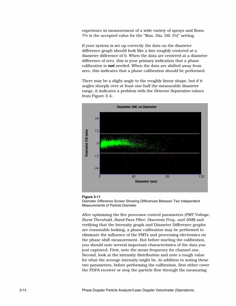
3-14 Phase Doppler Particle Analyzer/Laser Doppler Velocimeter (Operations)
experience in measurement of a wide variety of sprays and flows, 7% is the accepted value for the “Max. Dia. Dif. (%)” setting. If your system is set up correctly the data on the diameter difference graph should look like a line roughly centered at a diameter difference of 0. When the data are centered at a diameter difference of zero, this is your primary indication that a phase calibration is not needed. When the data are shifted away from zero, this indicates that a phase calibration should be performed. There may be a slight angle to the roughly linear shape, but if it angles sharply over at least one-half the measurable diameter range, it indicates a problem with the Detector Separation values from Figure 3-4.
Figure 3-11 Diameter Difference Screen Showing Differences Between Two Independent Measurements of Particle Diameter
After optimizing the five processor control parameters (PMT Voltage, Burst Threshold, Band-Pass Filter, Downmix Freq., and SNR) and verifying that the Intensity graph and Diameter Difference graphs are reasonable looking, a phase calibration may be performed to eliminate the influence of the PMTs and processing electronics on the phase shift measurement. But before starting the calibration, you should note several important characteristics of the data you just captured. First, note the mean frequency for channel one. Second, look at the intensity distribution and note a rough value for what the average intensity might be. In addition to noting these two parameters, before performing the calibration, first either cover the PDPA receiver or stop the particle flow through the measuring

Taking Size and Velocity Data 3-15
volume. You also need to perform the calibration with the optimized processor settings that you just used to capture your flow data.
R u n → C a l i b r a t i o n → L a s e r D i o d e C a l i b r a t i o n To start the calibration process select Run → Calibration → Laser Diode Calibration. A window will open like the one shown in Figure 3-12. To perform the calibration, enable the Cal. Diode checkbox and set the Doppler Frequency parameter to the mean frequency of the real flow. The value to enter will be that before downmixing, so you need to add the downmix frequency to the mean flow frequency. For example, if you had a mean flow frequency of 5 MHz and you were using a downmix frequency of 40 MHz, you would enter a Doppler Frequency of 45 MHz. Set the intensity to 100 and then take data like you would with a real flow. The Data Rate will be automatically calculated based on the chosen Doppler Frequency, and the Downmix Freq and Bandpass Filter settings from the Diameter Measurement screen.

3-16 Phase Doppler Particle Analyzer/Laser Doppler Velocimeter (Operations)
Figure 3-12 Calibration Diode Setup Page After Taking Calibration Data It would be very useful to open up the system graph showing the phase shifts for both detector pairs AB and AC. To do this go to Graphs → System Graphs → Phase AB, Phase AC. After taking a set of data, the graph should look something like the one shown in Figure 3-13.

Taking Size and Velocity Data 3-17
Figure 3-13 Typical Phase AB, Phase AC Graph After Capturing Calibration Diode Data In the Laser Diode Calibration page (Figure 3-12) both the Phase Mean and Phase RMS parameters should update after capturing data to reflect the mean and RMS of the two phase distributions (AB and AC). The mean values should be near zero (±30) for lower frequency flows. For higher frequencies (above 20 MHz) the phase mean values will gradually move further away from zero. The RMS values should typically be less than or around 3 degrees. In the example data shown in Figure 3-13 and Figure 3-14, the mean phase for AB is –0.37 degrees and the RMS is 1.17 The distribution for AC has a mean of –9.72 degrees and an RMS of 1.66 degrees. You should now check the intensity values by looking at the intensity versus size graph. There will probably be very few points on the graph, as most will be rejected as a particular error type. However, the few points there should be clustered around a certain intensity value. If this intensity is higher than the mean intensity value you noted from your real flow data, then you should lower the Intensity parameter below 100 and retake data. Keep lowering the Intensity until the two intensities are roughly the same. If the intensity from the calibration data is lower than the mean intensity data of your flow even with an Intensity parameter of 100 then you can stop. The phase calibration is actually affected very weakly by the signal intensity, so you can expect an accurate correction.
After checking the above you should copy the Phase Mean values for both the AB and AC distributions into the Phase Cal edit boxes. For the example we have been displaying, Figure 3-14 shows what the page should look like after copying the values. Uncheck

3-18 Phase Doppler Particle Analyzer/Laser Doppler Velocimeter (Operations)
(disable) the Enable Cal. Diode checkbox. You have now completed the calibration procedure.
Figure 3-14 Calibration Diode Setup Page After Copying the Mean Phase Values

4-1
C H A P T E R 4 Optimizing Particle Size Measurement and Obtaining Detailed Flow Information
After completing Chapters 1–3, you are ready to do the final capture of data with your PDPA system. Remember that the diode calibration was done in Chapter 3 with a particular set of processor parameters. If you change these you may need to do a new calibration. Using Graphs → … select the graphs that you want to view during data capture. From System Graphs menu, you may want to select Intensity Validation, Diameter Diff. Vs. Diameter, and Velocity vs Diameter. Other graphs of interest would be Diameter Histogram, Velocity, Frequency and Gate Time Histograms for the Channels in use. You may also want to display some of the numerical statistics as well. You are recommended to use Statistics → System Statistics and select Velocity Statistics, Diameter Statistics and Volume Distribution Statistics. You can arrange the graphs and statistics windows manually or use the options (Tile Horizontally, Tile Vertically or Cascade) available under menu item Window. Start a new run (see Chapter 1) and collect data by pressing <F9> or the Capture Run button on the main tool bar as shown in Figure 4-1.
Figure 4-1 Capture Run Button on the Main Tool Bar After capturing a run, you can examine the plots and statistics to decide whether this data makes sense. For example, the diameter difference should be small and velocity versus diameter should follow an expected trend (e.g., in the spray of a pressure atomizer, larger drops move faster due to higher inertia. Note: the white

4-2 Phase Doppler Particle Analyzer/Laser Doppler Velocimeter (Operations)
curve on the Velocity vs Diameter plot represents the average correlation). If you think that the collected data is valuable, it is advised that you save it immediately. For this purpose, use Run → Save Run or the Save button on the tool bar. Now your data cannot be overwritten and you cannot capture more data without creating a new run. However, you can playback the saved data and try out various data reduction options that are discussed below. When you have a reasonable looking intensity versus size plot (something similar to Figure 3-10), you can turn on the intensity validation. To do this go to the Intensity Validation/PVC tab found in the upper-right window of the main software screen. See Figure 4-2 for the contents of this page. To enable intensity validation click on the Enable Intensity Validation checkbox.
Figure 4-2 Settings to Utilize Intensity Validation and Probe Volume Correction As shown in Figure 3-10, the intensity-diameter relation has a natural upper limit that follows a d2 law (scattered light intensity

Optimizing Particle Size Measurement and Obtaining Detailed Flow
Information 4-3
being proportional to the square of particle diameter). However, there may be some out-liers that need to be eliminated by setting an upper threshold curve that closely matches the natural upper limit. The slope of the upper threshold curve may be calculated automatically by checking Enable Auto Intensity Limit Calculation. If this choice is made, the Number of Diameter Bins should be set to a large number, e.g., 100 or 200. (You may find the auto-intensity option convenient in at least getting close to the natural upper limit. Or, you may opt to use manual settings iteratively to arrive at the correct upper limit). When you choose auto-intensity option, the following message (Figure 4-3) may appear. Please activate software coincidence and/or software subrange using the guidelines given under Chapter 10.
Figure 4-3 Warning Message Pertaining to Auto-Intensity Option The d2 law is based on the geometrical optics and does not apply to very small particles. You can set a Minimum Diameter Limit (um) below which the d2 law is not applied. This parameter can be ascertained from the intensity versus diameter scatter plot or can be determined through light scattering simulations. The value of this parameter would typically be 1–5 µm. The Slope of Upper Intensity Curve (mV/um*um) needs to be specified for the manual intensity validation. A good start would be 1000/dmax*dmax, where dmax is the largest measurable diameter. Lower-to-Upper Intensity Ratio determines the position of the lower intensity threshold curve relative to the upper curve. This ratio is obviously less than 1. If it is too close to 1, a large amount of data would lie below the lower threshold and will be rejected. On the other hand, if it is too close to 0, some weak signals with erroneous particle size information would be included in the valid data set. Simulations have shown that a value of 0.1–0.2 is appropriate for this parameter. A physical interpretation of the above parameter is as follows. Signals from a given size particle have different intensities because

4-4 Phase Doppler Particle Analyzer/Laser Doppler Velocimeter (Operations)
they cross the Gaussian laser spot at different locations. Those going through the center of the Gaussian spot generate the strongest signal with the largest intensity. Those grazing the measurement volume at its 1/e2 limits will generate signals with an intensity that is 0.135 times the largest intensity. Hence, by setting the lower-to-upper intensity ratio at 0.2, we truncate the measurement volume to a spot smaller than the Gaussian spot. By setting the above ratio to 0.1, we truncate it to a spot somewhat larger than the Gaussian spot. Theoretically, the upper and lower intensity curves should have zero intercept. However, there may be some electronics-related offset in the measurement that may be corrected by setting the intercept to a non-zero value. In most applications the default value of zero would be satisfactory for Upper/Lower Intensity Curve Intercept. We do not recommend using an intercept outside the ±50 mV range. After entering appropriate intensity validation settings, press Apply (they are not applied automatically). You are now ready to playback the data just taken with intensity validation. Use the playback button from the main tool bar as shown in Figure 4-4.
Figure 4-4 Playback Button on the Main Tool Bar The intensity validation plot now has two white curves, showing the upper and the lower intensity thresholds. In agreement with the d2 law, these curves are parabolic. The upper curve becomes flat for the diameter values smaller than the Minimum Diameter Limit. The data points lying outside the two limiting curves are rejected and shown in red. You would notice changes in the Diameter Histogram and Diameter Statistics. You have probably gotten rid of some of the unrealistically large particles. This is a good time to review the information on the statistics displays.
Velocity Statistics, as shown in Figure 4-5, provides the mean and the root-mean-square (RMS) values of velocity for each component that is enabled. The Turbulence Intensity is the ratio of RMS to mean velocity expressed as a %. The mean, RMS and % fluctuation are also reported for the signal frequency. Note that the frequency includes a shift and the frequency statistics are not simply a scaling factor different from the velocity statistics.

Optimizing Particle Size Measurement and Obtaining Detailed Flow
Information 4-5
Channel 1 Channel 2 Channel 3Velocity Mean (m/sec)Velocity RMS (m/sec)Turbulence Intensity (%)Frequency Mean (MHz)Frequency RMS (MHz)Frequency TI (%)Gate Time Mean (usec)Gate Time RMS (usec)Data Rate (Hz)Valid CountInvalid CountElapsed Time (sec)
8.7320 0.4629 0.25842.3668 0.1029 0.121327.11 22.24 46.967.7461 7.3499 7.19951.6930 0.0778 0.093721.86 1.06 1.307.95 5.46 5.732.91 1.67 2.131795 2052 29683465 3465 34650 0 02.5373
Figure 4-5 Velocity Statistics The Velocity Statistics screen also reports the mean and RMS values of the “gate time.” The gate time represents the duration of the individual signals. This can be used as a check for the quality of the measurements. The gate time multiplied by the main velocity component results in a distance that should roughly represent the size of the measurement volume. If the above distance is too much smaller or larger than the nominal size of the measurement volume, one may expect some problems with the measurements. The gate time is also used for correcting the sampling bias in the velocity or probe volume bias in the size measurement. The Velocity Statistics screen also provides the Data Rate, the number of valid signals collected (Valid Count) and the total duration of the measurement (Elapsed Time). In velocimetry applications, a high data rate is desirable in order to resolve the fine time scales of turbulence. The valid count would vary from channel to channel, unless coincidence is enabled. In the case of coincidence, individual data rates are reported for each channel, but the valid count represents the coincident data only.
Invalid Count refers to the number of samples that were coincident but which did not result in a valid velocity. This category is relevant for hardware coincidence only.
The Diameter Statistics, as shown in Figure 4-6, consists of various mean diameters, i.e., number mean D10, surface mean D20, volume mean D30, Sauter mean D32 and D43. The following general definition applies to all of the above mean diameters:
nm
n
m
mn DD
D−
⎟⎟⎠
⎞⎜⎜⎝
⎛=∑∑
1
.

4-6 Phase Doppler Particle Analyzer/Laser Doppler Velocimeter (Operations)
Figure 4-6 Diameter Statistics The mean diameters are computed in three different ways. The first column represents the raw means, based on the data as it is. The second column is titled PVC, which stands for Probe Volume Correction. The effective probe volume in phase Doppler applications is a function of particle diameter. Large particles are able to scatter discernible signals from the outer regions of the measurement volume, where illumination intensity is weak due to the Gaussian distribution. On the other hand, small particles scatter less light per unit illumination. Hence, they generate measurable signals only from the central region of the measurement volume. This probe volume bias favors larger particles. It must be pointed out that the intensity validation tends to undo the above effect by validating signals within certain boundaries, regardless of the particle size. However, the probe volume bias may be present at the lower end of the size distribution. The values in the PVC column are zero, unless Enable Probe Volume Correction is checked on Intensity Validation/PVC screen. After probe volume correction, the mean values represent temporal averages; i.e., average values seen by an observer who is examining the particles passing by a given point in space. This observer sees more of the faster moving particles. Another kind of average is called spatial average (3rd column), which is seen by an observer who takes a snapshot of the entire particle field. This observer reports averages based on a region around the observation point that is large enough to provide good statistics. Spatial averages can be deduced from the PDPA data. Although the actual algorithm is quite complex, the basic idea is to use the transit time weighting in order to cancel out the bias towards the faster particles.
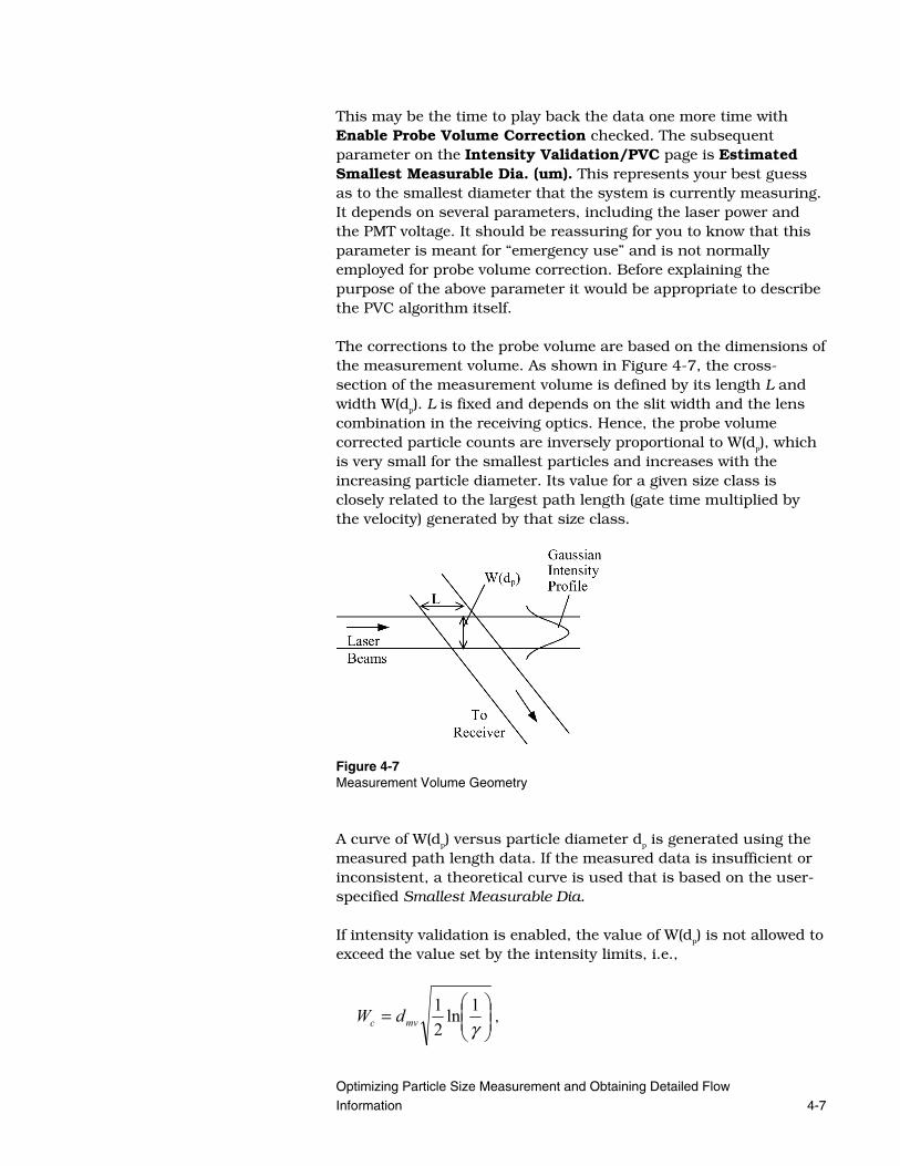
Optimizing Particle Size Measurement and Obtaining Detailed Flow
Information 4-7
This may be the time to play back the data one more time with Enable Probe Volume Correction checked. The subsequent parameter on the Intensity Validation/PVC page is Estimated Smallest Measurable Dia. (um). This represents your best guess as to the smallest diameter that the system is currently measuring. It depends on several parameters, including the laser power and the PMT voltage. It should be reassuring for you to know that this parameter is meant for “emergency use” and is not normally employed for probe volume correction. Before explaining the purpose of the above parameter it would be appropriate to describe the PVC algorithm itself. The corrections to the probe volume are based on the dimensions of the measurement volume. As shown in Figure 4-7, the cross-section of the measurement volume is defined by its length L and width W(dp). L is fixed and depends on the slit width and the lens combination in the receiving optics. Hence, the probe volume corrected particle counts are inversely proportional to W(dp), which is very small for the smallest particles and increases with the increasing particle diameter. Its value for a given size class is closely related to the largest path length (gate time multiplied by the velocity) generated by that size class.
Figure 4-7 Measurement Volume Geometry A curve of W(dp) versus particle diameter dp is generated using the measured path length data. If the measured data is insufficient or inconsistent, a theoretical curve is used that is based on the user-specified Smallest Measurable Dia. If intensity validation is enabled, the value of W(dp) is not allowed to exceed the value set by the intensity limits, i.e.,
⎟⎟⎠
⎞⎜⎜⎝
⎛=
γ1ln
21
mvc dW ,

4-8 Phase Doppler Particle Analyzer/Laser Doppler Velocimeter (Operations)
where mvd is the 1/e2 probe volume diameter and γ is the Lower-to-
Upper Intensity Ratio. When the data is played back with PVC enabled, several changes happen in the output. In the Diameter Statistics, non-zero values appear in the columns titled PVC and Spatial. You may notice your probe volume corrected mean diameters are about the same as the uncorrected values. This happens when the small particles do not play a significant role and the intensity validation based W is practically valid over the entire size range. In other words, intensity limits make the probe volume fixed and eliminate the probe volume bias.
If the small particles, with W values smaller than Wc, are significant, the probe volume corrected mean diameters are smaller than the uncorrected values. Figure 4-8 shows the Volume Distribution Statistics. Non-zero values are available here. The parameters x and q define the best fit of PVC corrected data to Rosin-Rammler distribution, given by
( )[ ]qxDexpQ −=−1
where Q represents the fraction of the total volume contained in drops of diameter less than D.
xqLWC (g/m3)Volume Flux X (cc/cm2 s)Volume Flux Y (cc/cm2 s)Volume Flux Z (cc/cm2 s)Volume 1% (um)Volume 10% (um)Volume 50% (um)Volume 90% (um)Volume 99% (um)Total Particle Conc.(1/cc)
40.922.75109.15430.11660.01580.00007.6918.0535.8155.4371.3310850.4639
Figure 4-8 Volume Distribution Statistics

Optimizing Particle Size Measurement and Obtaining Detailed Flow
Information 4-9
LWC represents the liquid water content in grams per cubic meter. It is based on the assumptions that the particles are water drops. For other kind of particles, multiply this number by the specific gravity of the particulate matter in order to determine the mass per unit volume of the particles. The x, y and z components of the flow rate of particle material per unit area are expressed as Volume Flux X, Y and Z, respectively. These components of the volume flux correspond to the first, second and third velocity component. Each component of volume flux is the summation of bin-by-bin volume fluxes for that component.
The bin-resolved x (y or z)-component of volume flux is given as the volume fraction times the mean x (y or z) velocity component for the size bin under consideration.
The volume fraction for the jth size bin is expressed as
TV
tDL
jprobe
jj
j_
3
6 ∑=
π
,
where summation is done for all the particle diameters jD and
their transit times jt in the jth size bin. T represents the total
measurement time and jprobeV _ is the volume of the probe region for
the jth size bin.
As discussed above, the effective volume of the probe region may increase with the increasing particle diameter, due to increasing signal strength. The following definition of jprobeV _ provides the
necessary size dependency of the probe region on the particle size,
jjrb
rfjprobe hW
ffs
V ⎟⎟⎠
⎞⎜⎜⎝
⎛=
φsin_ ,
where s, rff , rbf and φ are the slit width, focal length of the front
receiver lens, focal length of the back receiver lens and the collection (off-axis) angle, respectively. The term in the parentheses represents the length of the probe region, whereas jW and jh are
the size-dependent width and height of the probe region.
jh is the mean path length for the jth size class.
Referring to Figure 4-8, the following will describe the remaining parameters.

4-10 Phase Doppler Particle Analyzer/Laser Doppler Velocimeter (Operations)
Volume 1 represents the drop diameter in microns such that 1% of total liquid volume is in drops of smaller diameter. Volume 10 represents the drop diameter in microns such that 10% of total liquid volume is in drops of smaller diameter.
Volume 50 is the drop diameter in microns such that 50% of total liquid volume is in drops of smaller diameter. This is also referred to as the mass median diameter (MMD), or volume median diameter (VMD, MVD). Volume 90 represents the drop diameter in microns such that 90% of total liquid volume is in drops of smaller diameter. Volume 99 represents the drop diameter in microns such that 99% of total liquid volume is in drops of smaller diameter. The number of particles (all size bins) per unit volume in cc-1 is represented by Total Particle Conc. (1/cc). Further information about the particulate two-phase flow is given in the graph reached by Graphs → System Graphs → Particle Diameter Distribution. This plot Figure 4-9) has five size distributions. The first two histograms represent the uncorrected and probe volume corrected particle counts. The particle counts are normalized with the width of the size bin (in microns), so that the area under the curve is always 100%. In the case of Corrected Area and Corrected Volume curves, the vertical scale represents the surface area and the volume of the drops. Normally, the peak of the area distribution is shifted to the right of the number distribution and that of volume distribution is shifted to the right of the area distribution.

Optimizing Particle Size Measurement and Obtaining Detailed Flow
Information 4-11
Figure 4-9 Various Size Distributions The concentration distribution is also normalized with the bin width, so that the area under the curve represents the total concentration in 1/cc as given in Volume Distribution Statistics (Figure 4-8). All the distributions in Figure 4-9 represent the temporal data, except the concentration distribution, which is spatial by definition.
D i a m e t e r F i t t i n g There are five Diameter Fit Routines available to help transfer measured results to numerical models. Selection is made in the Diameter Measurement tab (Figure 3-7), press the Playback button to force FLOWSIZER to recompute the fit.
Rosin Rammler This is the most widely used expression for drop size distribution, although it was originally developed to approximate the crushing of solids into powders. It is expressed in the form:
qXDQ )/(exp1 −=−

4-12 Phase Doppler Particle Analyzer/Laser Doppler Velocimeter (Operations)
Where Q is the fraction of the total volume contained in drops of diameter less than D, and X and q are constants.
Fit Var: x in FLOWSIZER represents X.
Fit Var: q in FLOWSIZER represents Q.
Normal The Normal distribution function is based on processes that are random in nature and where no specific bias is present. Atomizers, humidifiers, and some air-assist spray generators produce normally distributed droplet diameters. This fit usually models the number distribution best.
⎥⎦
⎤⎢⎣
⎡−−== 2
2 )(21exp
21)( DD
ssDf
dDdN
nnπ
Where ns is a measure of the deviation of values of D from a mean
value D .
Fit Var: Mean in FLOWSIZER represents the mean value.
Fit Var: Variance in FLOWSIZER represents the deviation value.
Log Normal Many particle size distributions that occur in nature have been found to follow the Gaussian or Normal distribution law if the logarithm of the particle diameter is used as the variable. Pressure atomizers and hole-type fuel injectors typically have diameter distributions that follow this model. This fit does a better job of modeling the number distribution, rather than the volume distribution.
⎥⎥⎦
⎤
⎢⎢⎣
⎡−−==
−2
2 )ln(ln21exp
21)( ng
gg
DDsDs
DfdDdN
π
where ngD−
is the number geometric mean drop size and gs is the
geometric standard deviation.
Fit Var: Mean in FLOWSIZER represents the mean value.
Fit Var: Variance in FLOWSIZER represents the deviation value.
Fit Var: XBar = exp(Mean) in FLOWSIZER represents the exp of the mean value.
Figure 4-10 shows a Log-Normal Fit to a Diesel injectory spray.

Optimizing Particle Size Measurement and Obtaining Detailed Flow
Information 4-13
Matsumoto-Takahashi It is also known as Modified Log Normal. It is used when values of either Dmin or Dmax (or both) are known, and restrict the values of the particle sizes.
⎥⎥
⎦
⎤
⎢⎢
⎣
⎡
−
−−−== −2
max
maxmin2 )
)(
))(((ln21exp
21)(
DDD
DDDDsDs
DfdDdN
ng
Min
ggπ
Where maxD is the maximum diameter and minD is the minimum
diameter.
Fit Var: Mean in FLOWSIZER represents the mean value.
Fit Var: Variance in FLOWSIZER represents the deviation value.
Fit Var: XBar = exp(Mean) in FLOWSIZER represents the exp of the mean value.
Fit Var: Max in FLOWSIZER represents the maximum diameter.
Nukiyama-Tanasawa The expression contains two independent constants, namely b and q. This expression is sometimes found to be a better model for pressure atomizers and hole type fuel injectors, compared to the above models. It performs better as a volume distribution fit.
qbDDdDdN )(exp2 −=
Fit Var B = exp(r) in FLOWSIZER represents b.
Fit Var: q in FLOWSIZER represents Q. Two system graphs use the currently selected Diameter Fit routines (Figure 4-10 and Figure 4-11). These plots are accessed under Graphs → System Graphs → Diameter Distribution and Fit and Graphs → System Graphs → Volume Distribution and Fit. These system graphs allow you to view the number-based and volume-based distributions and fits.

4-14 Phase Doppler Particle Analyzer/Laser Doppler Velocimeter (Operations)
Figure 4-10 Diameter Distribution and Fit: Log Normal Screen
Figure 4-11 Volume Distribution and Fit: Rosin Rammler Screen The quality of fit is affected by the bin settings. Too many bins introduce artificial variations, too few bins mask the actual trends. Figure 4-12 shows an example fit with too many bins. Right-click on the plot, select Edit Histogram Data Sets... then select

Optimizing Particle Size Measurement and Obtaining Detailed Flow
Information 4-15
Diameter Count from the list. “Bin Count” should be set to give a “Bin Range” of about 1 µm/bin. Press OK when finished.
Figure 4-12 Volume Distribution and Fit: Nukiyama-Tanasawa Screen with Too Many Bins Figure 4-13 shows the result after going from 0.1 µm/bin (Figure 4-12) to 1.0 µm/bin.

4-16 Phase Doppler Particle Analyzer/Laser Doppler Velocimeter (Operations)
Figure 4-13 Volume Distribution and Fit: Nukiyama-Tanasawa Screen going from 0.1 µm/bin to 1.0 µm/bin
All the above discussion pertains to a single measurement point in a particle flow. In order to cover a flow field the above measurements need to be repeated at multiple points. The present software can control a traverse and automate the process of moving the measurement volume from one location to the other. See Chapter 13, “Setting up and Using a Traverse.” Sometimes you may want to correlate the size and velocity data with the measurements taken with other devices (e.g., pressure and temperature sensors). This is accomplished using the external input option discussed under Chapter 8, “Using External Input.” Many flows are periodic, e.g., a pulsed spray. FLOWSIZER software allows the analysis of periodic flows, i.e., phase averaging (see Chapter 12, “Using RMR”).

5-1
C H A P T E R 5 Selecting an Optical Layout for Particle Sizing
For particle sizing applications, it is important that the transmitting and the receiving probes are positioned correctly relative to each other, polarization is set right and the slope of the phase-diameter curve is specified correctly. FLOWSIZER helps to select the above parameters. To start using FLOWSIZER for this purpose, choose Run → Run Setup → Diameter Measurement. A dialog box, shown in Figure 5-1 appears. In order to use this utility, you should know the refractive index and light attenuation coefficient of the particles. If the particles are suspended in a liquid, the refractive index of the liquid is also needed. These data for some of the common materials is given in a table, which can be accessed by pressing the button labeled “Table.” It opens the dialog box shown in Figure 5-2. In many applications involving drops of special liquids, e.g., paints, adhesives, fuels, you have to measure the optical properties. An Abbe refractometer can be used to measure the refractive index. Attenuation coefficient α can be determined using measurement of the transmission of a laser beam through a liquid film of known thickness. The following correlation is used for this purpose:
L
in
out ePP α−= ,
where inP and outP are the laser power entering and leaving the
liquid film respectively. L is the thickness of the film.

5-2 Phase Doppler Particle Analyzer/Laser Doppler Velocimeter (Operations)
Figure 5-1 Main Dialog Box for Selecting the Optical Layout
Figure 5-2 Optical Properties of Common Particle Materials

Selecting an Optical Layout for Particle Sizing 5-3
You should proceed with the following steps to select the optical arrangement: 1. Enter the values of Refractive Index of the Particle, Refractive
Index of the Medium and the Attenuation Coefficient on the Diameter Measurement page of Run Setup. Now, hit Apply and the values of the Attenuation Level and the Relative Refractive Index will be updated. Attenuation Level is based on the product of Attenuation Coefficient and the Maximum Expected Particle Diameter. It is read from the following table.
Attenuation
Level ( ) ( ) 1000μmmm max
1pd×−α
1 < 0.005
2 0.005—0.05
3 0.05—500
4 500—4000
5 > 4000
Relative refractive index is the ratio of the particle refractive index to the medium refractive index.
2. Click on the button labeled Domains. The graph of Figure 5-3
will appear.
Figure 5-3 Scattering Domains Covering a Wide Range of Relative Refractive Indices and Off-Axis Angles

5-4 Phase Doppler Particle Analyzer/Laser Doppler Velocimeter (Operations)
At this point, you should select one are more domains that are available for the present application. For most liquid sprays in a gaseous environment, the relative refractive index is 1.3–1.4, so that the scattering domains 8–12 are available for further evaluation. If you do not have optical access in the near forward direction (i.e., off-axis angles <90° are not available), only Domain 8, 9, and 10 would be available. For gas bubbles in a liquid, the relative refractive index would be in the range of 0.7 to 0.8, making scattering domains 2–7 available for further evaluation.
3. Click on the button labeled “Modes.” This will display the Scattering Mode Charts, as shown in Figure 5-4. The two charts pertain to the two cases of polarization of light. Standard TSI systems use perpendicular polarization, meaning the electric vector is perpendicular to the beam plane. You can now examine the scattering mechanisms pertaining to the present set of domains and the attenuation level.
Circles, triangles and squares are used to represent the scattering mechanisms of reflection, refraction and internal reflection, respectively. Closed symbols mean a high level of confidence in the choice of the scattering mechanism. In this case, FLOWSIZER will compute the slope of the phase-diameter curve using both geometric and Mie-based light scattering theories. Open symbols signify a lower level of confidence and the estimated slope may deviate by more than 5% from the actual slope. In this case, it is recommended that you use a more rigorous theory of light scattering, i.e., Mie theory, to examine the phase-diameter relationship. Contact TSI if you think this is needed.

Selecting an Optical Layout for Particle Sizing 5-5
Figure 5-4 Feasible Scattering Modes for Various Domains, Attenuation Levels and Polarization
Let us consider a few examples. For water drops in air, the attenuation level is 1 and the available modes are 8–12. The scattering mode charts show that perpendicular polarization and domain 11, with refraction as the scattering mechanism, are the best choice. You can also use domain 8 or 9, if domain 11 is not available due to some physical constraints in the experimental setup. For air bubbles in water, parallel polarization (i.e., polarization in the beam plane) and domain 6 offer a good combination. Normally, PDPA systems are built to have electric vector of polarization perpendicular to the plane of the laser beams (2nd chart). If parallel polarization is needed, contact TSI for a modification of your fiberoptic couplers to enable switching of the polarization. Another choice for bubble sizing is Domain 2 with either case of polarization. For particles with attenuation level of 5, e.g., metallic particles, surface reflection is the only scattering mechanism and hence, any domain or polarization can be used.

5-6 Phase Doppler Particle Analyzer/Laser Doppler Velocimeter (Operations)
Most paints and fuels have attenuation levels of 1 or 2 and hence, domain 11 and perpendicular polarization are feasible. Also, due to their higher refractive index, backscatter modes 8 and 9 are usually not available. Very opaque fluids, with attenuation levels of 3 or 4, can only be measured in Domain 10 with parallel polarization.
4. So far we have selected the scattering mechanism and the
polarization angle. These may be entered on the Diameter Measurement page. We also know the scattering domain, which restricts the choice of off-axis angles to a certain range (see Figure 5-3). For water drops in air (relative refractive index: 1.33), if Domain 11 is selected, the available off-axis angles are 30-75°. It is your choice to select one of these angles. It is preferable to be well inside the domain and not too close to the boundaries. For air bubbles in water (relative refractive index: 0.75), domain 2 requires the off-axis angle to be in 60–80° range and domain 6 restricts it to 80–90°. Domain 2 is a better choice, because signals are stronger and the standard case of polarization, i.e., perpendicular, can be used. Enter the selected off-axis angle on the Diameter Measurement page.
5. With all the entries current on the Diameter Measurement page, click Auto Slope. This will compute the non-dimensional slope of the phase-diameter curve, defined through the following relationship:
Spacing Fringe DiameterParticle
LengthocalReceiver FSeparationDetector Slope""
360Phase ××=
A message will appear on the message screen (bottom right corner of the FLOWSIZER screen). This message may read, “Orient the PDPA receiver in its ring mounts, such that the white arrow seen through the eye piece, points in the positive flow direction,” or, “Orient the PDPA receiver in its ring mounts, such that the white arrow seen through the eye piece, points against the positive flow direction.” The positive flow direction is from unshifted to shifted beam, that is, against the fringe motion. All cases of external reflective

Selecting an Optical Layout for Particle Sizing 5-7
scatter, including Domain 2 for bubbles, use the arrow pointing against the positive flow direction. All cases of refraction, including internal reflection, use the white arrow pointing in the positive flow direction. During the installation of the system, you may have already set the “white arrow” in the right direction. If you are not sure how to do this, please consult the installation manual. If the entries on the diameter measurement page are not self-consistent, you may get a message like the one shown in Figure 5-5. Please revisit Figure 5-3 and Figure 5-4 and make sure that your entries are consistent.
Figure 5-5 Error Message Pertaining to Inconsistent Entries for Auto Slope
Slope can also be entered manually. This would be the case when Mie scattering calculations show a slope significantly different than the Auto Slope.
6. Hit Apply and switch to the Optics page of Run Setup. You will see an updated value of Diameter Limit Max (um). If it is less than your expected maximum, you should change at least one of the following optical parameters in the suggested manner:
Increase the Transmitter Focal Length; Reduce the Beam Separation (for example, using a
Model XPD50-I beam expander in 0.5:1 contraction position);
Increase the Receiver Front Lens focal length The relationship between the above parameters and the maximum diameter is linear, i.e., doubling the transmitter focal length would double the size range. Reducing the beam separation to half would have the same effect. You may also want to modify the optics if Diameter Limit Max (um) is much larger (more than twice) the expected maximum diameter.

5-8 Phase Doppler Particle Analyzer/Laser Doppler Velocimeter (Operations)
Contact TSI for the available choices of the transmitter and receiver lenses as well as the beam expanders.
The above steps should complete your selection of the optical layout for particle sizing. You may still have to do the necessary hardware changes and optical alignments before proceeding with the measurements.

6-1
C H A P T E R 6 Creating and Using Graphs
The graphing capabilities of the FLOWSIZERTM Data Acquisition and
Analysis Software add a unique dimension of flexibility to the software. You can create histogram plots, scatter plots, smoothed line plots, etc. After creating a plot, it is immediately available in a drop-down list. The FLOWSIZER graphing system is based on a set of variables—some measured, some derived—that can be plotted one versus another, as you choose.
S h o w i n g a G r a p h Press <Alt><G> (or Graphs) and use the Up/Down arrow keys or click the Graphs menu item to select an existing graph. Seven graphs located in the System Graphs submenu are pre-defined because of their importance to phase/Doppler applications. These include the Intensity Validation graph, Diameter Difference vs Diameter graph, Phase AB Phase AC graph, Velocity vs Diameter plot, Particle Diameter Distribution graph, Diameter Distribution and Fit graph, and Volume Distribution and Fit graph. All user-defined graphs are listed below the System Graphs submenu. Simply select the one you wish to display. The current data needs to be replayed, or, new data acquired, to appear in the graph. Each graph entry in the Graph menu corresponds to a pair of files in the current Project folder. A graph named Diameter Histogram, for example, is associated with the file pair Diameter Histogram.grf and Diameter Histogram.bin. If you create a new Project folder, the existing graphs can be copied into it so that you don’t have to redesign all the graphs. A variety of plots are included with FLOWSIZER, but oftentimes you will need to display other data by creating a new graph. The following section will guide you through this process.

6-2 Phase Doppler Particle Analyzer/Laser Doppler Velocimeter (Operations)
D e s i g n i n g a G r a p h Press <Ctrl><G>, or select Graphs → Graph Designer, or press the Graph Designer button (shown in Figure 6-1) to design your own graph. The dialog shown in Figure 6-2 will appear.
Figure 6-1 Graph Designer Button Press the New button to bring up a dialog box so you can begin to create a new graph. You will first be prompted to enter a title for the new plot, then you will be returned to Figure 6-2 to select the plot style and variables. First select the Graph Type to create—either XY or Histogram. XY plots can have a variety of styles, including Line, Line + symbol, Scattered, Vert Bars, Horiz Bars, 3D Ver Bars, 3D Horz Bars. Next, from the Data Set column, select the variable to plot on each axis (XY plot) or the variable to display in a histogram. X and Y values can be scaled up or down by the Scale Factor. You may also modify the maximum number of data points to be displayed on the graph. Remember that this is independent of the Maximum Particle Measurement Attempts in the (Run → Run Setup) Run Settings tab. Finally, press Save to save your plot, and Close to return to FLOWSIZER.

Creating and Using Graphs 6-3
Figure 6-2 Graph Designer Screen
D e l e t i n g a G r a p h Press <Ctrl><G>, or select Graphs → Graph Designer, or press the Graph Designer button (shown in Figure 6-1). The dialog shown in Figure 6-2 will appear. Highlight the graph you wish to delete. Press the Delete button. This will delete the graph currently highlighted.
M o d i f y i n g a G r a p h Press <Ctrl><G>, or select Graphs → Graph Designer, or press the Graph Designer button (shown in Figure 6-1). The dialog shown in Figure 6-2 will appear. Highlight the graph you wish to modify. You are now free to alter the graph type, X and Y Data Set, X and Y Label, and Scale Factor. You may also modify the maximum number of data points to be displayed on the graph. Remember that this is independent of the Maximum Particle Measurement Attempts in the (Run → Run Setup) Run Settings tab. Press Save to save your changes.

6-4 Phase Doppler Particle Analyzer/Laser Doppler Velocimeter (Operations)
M o d i f y i n g a H i s t o g r a m D a t a S e t Right-click on any graph, or press the histogram Data Sets button in the Graph Designer Screen. The dialog shown in Figure 6-3 will appear. Highlight the histogram data set you wish to modify. You are now free to alter the Maximum, Minimum, and Bin Count. Using an excessively large bin count can cause meaningless features (peaks, gaps, etc.) to appear in the histogram.
Figure 6-3 Edit Histogram Data Sets Screen
Note: Several data sets are dependent on the Diameter Count Histogram settings. Changing the Diameter Count settings will change the settings for the dependent data sets automatically.

Creating and Using Graphs 6-5
C u s t o m i z i n g a G r a p h You can modify graph titles, axis labels, and even the graph type by double-clicking on the graph object you wish to modify. By double-clicking the graph title or an axis title, you can access the Text Parameters dialog box, shown in Figure 6-4. The title or label itself, and the font parameters can be modified here.
Figure 6-4 Text Parameters Dialog Double-clicking a plot axis (not the labels), brings up the axis edit dialog box. Figure 6-5 shows the Horizontal Axis dialog (the Vertical Axis dialog is similar). Axis limits are specified in the From/To fields. Enable Fixed Range to lock in the limits you specify when replaying the data and taking new data. Click the Line Attributes button to modify the axis line. Tick intervals and gridlines can be specified in the lower part of the dialog. The gridline style can also be modified if gridlines are enabled.

6-6 Phase Doppler Particle Analyzer/Laser Doppler Velocimeter (Operations)
Figure 6-5 Horizontal Axis Dialog Double-clicking the axis labels (the numbers near major tick marks) brings up the Text Parameters dialog box, shown in Figure 6-6. The position, format, and font format can be modified here.
Figure 6-6 Axis Labels Dialog

Creating and Using Graphs 6-7
Double-clicking a histogram graph (on the bars themselves) brings up the Bar Graph Parameters dialog box, shown in Figure 6-7. The type, format, position, and color can be set in this dialog. Pressing the Data button brings up a spreadsheet-like display of the actual data plotted. This useful feature will be explained in more detail later.
Figure 6-7 Bar Graph Parameters Screen Double-clicking any non-histogram graph (on the points or line) brings up the Plot Parameters dialog box, shown in Figure 6-8. The plot type and other attributes can be set in this dialog. Pressing the Data button brings up a spreadsheet-like display of the actual data plotted. This useful feature will be explained in more detail later.

6-8 Phase Doppler Particle Analyzer/Laser Doppler Velocimeter (Operations)
Figure 6-8 Plot Parameters Screen By right-clicking on a graph and selecting Edit Graph → Edit Graph Window you can edit the graph window attributes. A dialog will appear, as shown in Figure 6-9. This important dialog allows you to alter the plot color scheme if, for example, you are pasting plots into a word processing type application where a black background is undesirable.
Figure 6-9 Graph Parameters Screen
Left-click on or near any point or bar of a plot to view the coordinates (X and Y value) of that point in a floating information box, as shown in Figure 6-10. This is a useful way to identify peaks

Creating and Using Graphs 6-9
in histograms, and outliers in scatter plots, as well as other plot features.
Figure 6-10 Diameter Histogram Screen with Information Box Right-click on a graph and select Edit Graph → Edit Plot and then click the Data button to bring up the actual data in a spreadsheet-like window. Use Copy to copy the data and paste it into a spreadsheet application like Excel.
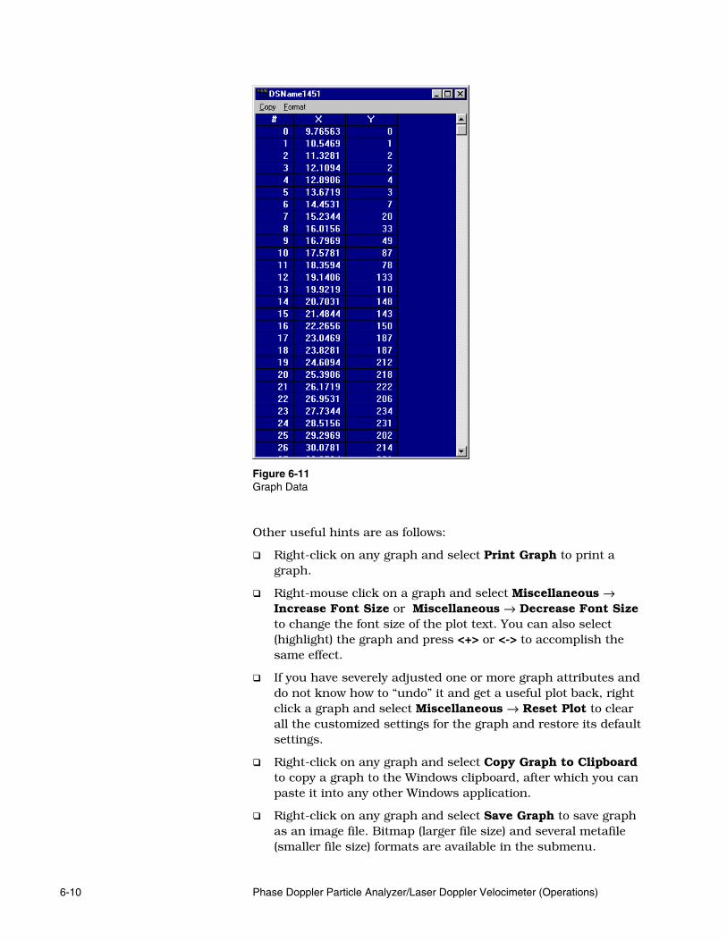
6-10 Phase Doppler Particle Analyzer/Laser Doppler Velocimeter (Operations)
Figure 6-11 Graph Data Other useful hints are as follows:
Right-click on any graph and select Print Graph to print a graph.
Right-mouse click on a graph and select Miscellaneous → Increase Font Size or Miscellaneous → Decrease Font Size to change the font size of the plot text. You can also select (highlight) the graph and press <+> or <-> to accomplish the same effect.
If you have severely adjusted one or more graph attributes and do not know how to “undo” it and get a useful plot back, right click a graph and select Miscellaneous → Reset Plot to clear all the customized settings for the graph and restore its default settings.
Right-click on any graph and select Copy Graph to Clipboard to copy a graph to the Windows clipboard, after which you can paste it into any other Windows application.
Right-click on any graph and select Save Graph to save graph as an image file. Bitmap (larger file size) and several metafile (smaller file size) formats are available in the submenu.

Creating and Using Graphs 6-11
By double-clicking on the title bar of a plot window, you toggle the plot window between full screen size and current size.
Press <Ctrl><H> or select Graphs → Tile Graphs Horizontally to horizontally arrange all the graphs and statistics windows in your display.
Select Graphs → Tile Graphs Vertically to vertically tile all graphs and statistics windows in your display.
Select Graphs → Cascade Graphs to cascade all graphs and statistics windows.
Select Graphs → Hide All Graphs to hide all graphs and statistics windows in your display.


7-1
C H A P T E R 7 Creating and Using Statistics Windows
The statistics capabilities of TSI’s FLOWSIZERTM Data Acquisition and
Analysis Software are very similar to the graphics capabilities, and so you can expect to become proficient rather quickly. The FLOWSIZER statistics system is based on a set of variables—some measured, some derived—that can be displayed in user-defined windows that can be moved and resized just like graph windows.
S h o w i n g a S t a t i s t i c s W i n d o w Press <Alt><S> and use the Up/Down arrow keys or click the Statistics menu item to select an existing statistics window. As shown in Figure 7-1, six statistics windows located in the System Statistics submenu are pre-defined because of their importance. These include:
Velocity Statistics
Diameter Statistics
Volume Distribution Statistics
Velocity and Size Subrange Statistics
External Input Subrange Statistics
Velocity Transformed Statistics Any or all these can be displayed as you choose.
Figure 7-1 Statistics Selection Menu

7-2 Phase Doppler Particle Analyzer/Laser Doppler Velocimeter (Operations)
V e l o c i t y S t a t i s t i c s W i n d o w Figure 7-2 shows the Velocity Statistics Window. Three-channel coincident data are shown in this example.
Channel 1 Channel 2 Channel 3Velocity Mean (m/sec)Velocity RMS (m/sec)Turbulence Intensity (%)Frequency Mean (MHz)Frequency RMS (MHz)Frequency TI (%)Gate Time Mean (usec)Gate Time RMS (usec)Data Rate (Hz)Valid CountInvalid CountElapsed Time (sec)
8.7320 0.4629 0.25842.3668 0.1029 0.121327.11 22.24 46.967.7461 7.3499 7.19951.6930 0.0778 0.093721.86 1.06 1.307.95 5.46 5.732.91 1.67 2.131795 2052 29683465 3465 34650 0 02.5373
Figure 7-2 Velocity Statistics Window
D i a m e t e r S t a t i s t i c s W i n d o w Figure 7-3 shows the Diameter Statistics Window. The software algorithms require you to select coincident mode and enable the probe volume correction (PVC) algorithm in order to see the PVC and Spatially corrected values. Otherwise, they are all zeros.
Figure 7-3 Diameter Statistics Window

Creating and Using Statistics Windows 7-3
V o l u m e D i s t r i b u t i o n S t a t i s t i c s W i n d o w Figure 7-4 shows the Volume Distribution Statistics Window. The software algorithms require you to select coincident mode and enable the probe volume correction (PVC) algorithm in order to see these values. Otherwise, they are all zeros.
xqLWC (g/m3)Volume Flux X (cc/cm2 s)Volume Flux Y (cc/cm2 s)Volume Flux Z (cc/cm2 s)Volume 1% (um)Volume 10% (um)Volume 50% (um)Volume 90% (um)Volume 99% (um)Total Particle Conc.(1/cc)
5.032.600.00930.00010.00000.00000.862.124.376.939.05584.8448
Figure 7-4 Volume Distribution Statistics Window
V e l o c i t y a n d S i z e S u b r a n g e S t a t i s t i c s W i n d o w
Figure 7-5 shows the Velocity and Size Subrange Statistics Window. The software algorithms require you to select subranged mode and enter appropriate subrange values in order to see these values. Otherwise, they are all zeros. Refer to Chapter 10 for more details on how to use the subrange feature.
Figure 7-5 Velocity and Size Subrange Statistics Window

7-4 Phase Doppler Particle Analyzer/Laser Doppler Velocimeter (Operations)
E x t e r n a l I n p u t S t a t i s t i c s W i n d o w Figure 7-6 shows the External Input Subrange Statistics Window. Here you have to be using the external input option, and enter appropriate subrange values. Otherwise, they are all zeros, as they are here, since an external input option was not used.
Figure 7-6 External Input Subrange Statistics Window
T r a n s f o r m e d V e l o c i t y S t a t i s t i c s W i n d o w Figure 7-7 shows the Transformed Velocity Statistics Window. The software algorithms require you to select coincident mode and use a multi-channel PDPA or LDV. Otherwise, the results shown are not very meaningful, as they are here, since a 1D system was used for this data.
Figure 7-7 Transformed Velocity Statistics Window

Creating and Using Statistics Windows 7-5
Customizing a Statistics Window You can modify the appearance and colors used in statistics windows. Right-click in the window and select Edit Statistics → Edit Statistics Window... (Figure 7-8). Customize the colors used in the “Graph Parameters” window. Select OK when done.
Figure 7-8 Customizing a Statistics Window
Statistics Output Options Statistics windows can be copied and pasted into graphics software applications using the right-click Copy Statistics to Clipboard (Bitmap) option. When you want to copy statistics to other applications such as Microsoft Word, Excel, or PowerPoint, the Copy Statistics to Clipboard (Tabbed Text) option gives better results (Figure 7-9).

7-6 Phase Doppler Particle Analyzer/Laser Doppler Velocimeter (Operations)
Figure 7-9 Statistics Output Options Window Like Graph windows, Statistics windows can be saved to a variety of bitmap and metafile type files. These options are available under the right-click Save Statistics selection.
Statistics Summary Report All the above diameter, volume, velocity and transformed velocity statistics are also available in an ASCII (text) based screen. Select File → Statistics Report. The report can be printed, saved, or <Ctrl><C> copied to the clipboard. The contents of the Statistics Summary Report are shown in Figure 7-10, Figure 7-11, and Figure 7-12.

Creating and Using Statistics Windows 7-7
Figure 7-10 Statistics Summary Report #1

7-8 Phase Doppler Particle Analyzer/Laser Doppler Velocimeter (Operations)
Figure 7-11 Statistics Summary Report #2
Figure 7-12 Statistics Summary Report #3 A variety of statistics windows is included with FLOWSIZER, but oftentimes you will need to display your own set of statistics. One reason may be that the statistics useful to you happen to be

Creating and Using Statistics Windows 7-9
scattered among many system statistics windows, which leads to an extremely cluttered display. The following section will guide you through the process of creating your own Statistics Window.
D e s i g n i n g a S t a t i s t i c s W i n d o w Press <Ctrl><G>, or select Statistics → Statistics Designer, or press the Statistics Designer button (shown in Figure 7-13) to design your own graph. The dialog shown in Figure 7-14 will appear.
Figure 7-13 Statistics Designer Button Press the New button to bring up a dialog box so you can begin to create a new statistics window. You will first be prompted to enter a title for the new statistics window, then you will be returned to Figure 6-2 to select the variables to include. First, increment the number of rows and columns to make room for your data. Next, from the second column, select the variable to show using the drop-down menu. Enter a name for it in the left field. Repeat this for each item you wish to include. Finally, press Save to save your statistics window, and Close to return to FLOWSIZER.

7-10 Phase Doppler Particle Analyzer/Laser Doppler Velocimeter (Operations)
Figure 7-14 Statistics Designer Screen
E x a m p l e S t a t i s t i c s W i n d o w s Figure 7-15 shows two example statistics windows for 1D PDPA. The first is a convenient and compact grouping of some basic measured parameters. The second is a collection of PDPA rejections—useful to monitor while taking data to maintain reliability of the results.
Figure 7-15 Example Custom Statistics Windows

8-1
C H A P T E R 8 Using External Input
This chapter briefly covers the approach to input external data (Analog or Digital). The first screen is found under Run → Run Setup. Then select the External Input tab, as shown in Figure 8-1.
Figure 8-1 External Input Screen If RMR is enabled and the timestamp is reset each cycle, Digital Channel 1 will not be available for use. Four channels of analog and/or digital data can be captured and tagged with the selected velocity data.

8-2 Phase Doppler Particle Analyzer/Laser Doppler Velocimeter (Operations)
A n a l o g If each channel data taking is to be triggered along with Vel. Channel 1 data, select the row of boxes for Channel 1. If external data taking is to be synchronized with other Velocity channels, select the appropriate boxes (please note that Figure 8-1 shows only two velocity channels—i.e., 2D LDV/PDPA system).
The incoming external signal voltage can be converted to a range of values. To do this the following items need to be selected.
Converted Low Set this to be the low value for the converted signal for the external input channel. For example, the low value can be set to zero for the minimum input voltage.
Converted High Set this to be the high value for the converted signal for the external input channel. For example, the high value could be set to 100. If the converted low value is zero, you would then have values ranging from 0–100, similar to a “percent full-scale” reading.
Modulus Modulus needs to be selected as a number between the Converted Low and Converted High values. For example, if this value is selected as 50, the Converted values go from 0 to 50 as the input voltage goes from the minimum value (0 volts) to midrange (2.5 volts). As the input voltage crosses the mid range, the converted values again go from 0 to 50 (instead of 51 to 100). In other words, the converted values show “two cycles.” Selecting the modulus to be 25 would generate 4 cycles (the maximum converted value would be 25, for this case). Default value of –1 indicates that this feature is inactive.
Offset The offset value selected is added to the converted values.
Analog Input Range Analog Input range shows the range of analog voltage signals that the External Input will measure. These values correspond to the

Using External Input 8-3
Converted Low and Converted High values. The three ranges available are 0–5 volts, –5 to 5 volts and 0–10 volts.
D i g i t a l The setup procedure here is the same as that for Analog signals. Converted Low and Converted High are the low and high-end converted values corresponding to input digital signals of 0 and 216 (65,536).


9-1
C H A P T E R 9 Power Spectrum Analysis
This chapter briefly covers the approach to get the power spectrum of the velocity field. Since particle arrivals (at the measuring volume) occur at random times the velocity output from the signal processor is random. This makes the Spectrum analysis of LDV data different from standard approaches. The first screen is found under Run → Run Setup. Then select the Power Spectrum/Correlation tab, as shown in Figure 9-1.
Figure 9-1 Power Spectrum/Correlation Screen To do the spectrum analysis, first select Enable Power Spectrum/Correlation Analysis.

9-2 Phase Doppler Particle Analyzer/Laser Doppler Velocimeter (Operations)
Use Transformed Velocities; allows computation of the power spectrum of the velocity components after the matrix transformation (see Figure 9-2).
Figure 9-2 Processor/Matrix Screen Vector to Analyze: Velocity component or components whose power spectrum needs to be computed.
Analyze Method: There are two methods of analysis—Slot Analysis and Even-Time Analysis.
Slot Analysis: This method allows for the random arrival of velocity data. The process involves first a computation of the autocorrelation of raw data. This would generate an Autocorrelation function with random values of the time delay. This Autocorrelation function is “binned” to have equal dT values. In other words, the autocorrelation values are computed for equally spaced delay times. Fourier transform of this provides the power spectrum values. Please see Appendix B for more details on the technique.
Power Spectrum Analysis 9-3
Even-Time Analysis - Data needs to be collected in Even-Time Sampling mode (See Figure 9-2). This approach is used when the data rate high enough so that even-time sampling mode of data collection would be feasible—i.e., there is a new data point every time the sampling is done. This approach would not need Velocity bias correction to compute the statistics. Slot Analysis is the default Analysis Method.
Windowing Method: Lists the different windows that can be selected for FFT. Default selection is Hanning. You can also select No Windows.
Points per FFT: The range of values are 512–4096. As this value increases, the frequency resolution also increases. Default value is 512.
Enable Range Limits: Selecting this option would allow you to select portions of the data file to compute the spectrum. For example, selecting this option and choosing Start to be 1 and Stop to be 1024 would result in computing spectrum for the first 1024 points. If this is not selected, the entire data file (in blocks of 512) will be used for the computations.
Slot Analysis Options include:
Auto (Avg TBD): Selecting this would estimate the average dT for Autocorrelation to be computed from the average value of time between data (TBD). This is the default selection.
Correlation dT: If Auto (Avg TBD) was not selected, the value for Correlation dT (in microseconds) needs to be entered manually. The Autocorrelation function will be “binned” into an equally spaced distribution based on this value of dT.
50% Overlap: Choosing this will generate the Autocorrelation function using 50% overlap of the data.
Increment: Increment of 1 uses all the data to compute the Power Spectrum. Increment of 2 implies that every other data point will be skipped. In this case, only half the number of data points would be used for computing the spectrum. This approach could be used to get higher resolution at the lower end of the frequency spectrum, provided that a large number of data points have been collected.


10-1
C H A P T E R 1 0 Using Subrange, Coincidence Modes and Even-Time Sampling
The FLOWSIZERTM Data Acquisition and Analysis Software can
process and display your data in three different ways. By default, all the data that the processor can process are transferred to the host computer via the FireWire interface. FLOWSIZER displays this data as you acquire it, and it is also displayed during Playback. This means, using a 2D PDPA example, that a droplet could pass through the measurement volume and only allow a U component velocity measurement to be made (i.e., no diameter, no V velocity component). The default FLOWSIZER view (i.e., neither Subrange nor Coincidence button selected) would show the U velocity measurement in all the U velocity plots and histograms, even though its accompanying diameter and V velocity measurement cannot be included anywhere. This is often not desirable, such as when looking for diameter-velocity correlations, or velocity-velocity correlations. For these situations, the data can be “filtered” or “sorted” to select only those particles with no missing measurements—in the 2D PDPA example, the Diameter, U component velocity, and V component velocity must all be present. This is known as coincident data, and is explained in more detail later in this section. The data can also be “filtered” or “sorted” to select only those particles whose diameter, velocity, etc. fall within certain limits. This is known as subranged data and is explained in the following paragraphs. No data is ever deleted or lost when using the subrange and/or software coincidence features. It is simply not shown. The analysis capabilities of FLOWSIZER are very powerful, and part of that power comes from the capability to set limits on a measured variable and then investigate other measured data that falls inside those limits. To do this, we need to use both Subrange AND Coincidence buttons in FLOWSIZER. Subranging sets bounds for the variables we are examining. Coincidence sorts out all the other data so that we are left with only those that are associated with data within the subrange.

10-2 Phase Doppler Particle Analyzer/Laser Doppler Velocimeter (Operations)
You may have a 1D PDPA system, for example, and measure a velocity histogram with two distinct peaks. You ask whether the flow really has a bimodal velocity distribution, and if it does, is each peak associated with different diameter characteristics? The lower velocity peak may be associated with a larger droplet diameter, for example. You may have a 2D PDPA system, for example, and measure a transient (pulsed) spray. The independent variable in this case is time, specifically time After Start of Injection (ASOI). The axial velocity will vary greatly with time ASOI, initially being very high (near the nozzle exit velocity, depending on how far from the nozzle you are measuring) and after injection stops, decaying exponentially. The diameter and radial velocity will also vary greatly with time ASOI. You will want to subrange out various portions of the injection process to examine the diameter during actual injection, for example. You may also need to quantify the entrainment of ambient gas by examining the radial velocity during and/or after the actual injection process. You may want to examine the diameter of droplets entrained into the spray after injection stops. Subranging and coincidence allows you to investigate these types of questions and analyze your data quickly and in great depth.
I n p u t t i n g S u b r a n g e V a l u e s Click the Subranges (Over/Under) tab in the controls area (right part of the FLOWSIZER window). As shown in Figure 10-1, five measured parameters can be subranged. These include:
Velocity
Gate Time
Diameter
Intensity
Time If the system is equipped with the External Input option, four additional analog and four additional digital subrange inputs are also available. The system shown in Figure 10-1 was not equipped with the External Input option, so the relevant fields are disabled.
For each variable, you can select a lower limit only, an upper limit only, or both an upper and lower limit.

Using Subrange, Coincidence Modes and Even-Time Sampling 10-3
Figure 10-1 Subrange Input Menu
E x a m p l e S u b r a n g e A n a l y s i s Figure 10-2 shows the Velocity and Diameter Histogram Windows for a 2D PDPA run with a bimodal U velocity histogram. In this section, we will analyze this data using subranges, to show the capabilities of subrange analysis.

10-4 Phase Doppler Particle Analyzer/Laser Doppler Velocimeter (Operations)
Figure 10-2 Diameter and Velocity Window for Subrange Example
V e l o c i t y S u b r a n g e The descriptive statistical variables describing a bimodal velocity distribution, such as that shown in Figure 10-2, may not be very meaningful. In this case, we can subrange the Channel 1 Velocity between the two peaks—or, at 5.6 m/s in this example. We then have two populations or “subranges,” one below 5.6 m/s and one above 5.6 m/s. We will use only the U Velocity (Channel 1) subrange. Figure 10-3 shows the FLOWSIZER Window. All the results displayed here are associated with only those particles having a velocity under 5.6 m/s, i.e., those in the lower peak. Note the following:
A value of 5.6 m/s is entered in the subrange on the right
The Subrange button is pressed
The Coincidence button is pressed
Only the lower channel 1 velocity peak is present
These slower-moving droplets tend to be smaller

Using Subrange, Coincidence Modes and Even-Time Sampling 10-5
Figure 10-3 FLOWSIZER Window for Lower Velocity Subrange Next we will examine the particles in the upper channel 1 velocity peak. Figure 10-4 shows the FLOWSIZER window for this data. All the results displayed here are associated with only those particles having a velocity above 5.6 m/s, i.e., those in the upper peak. Note the following:
A value of 5.60001 m/s is entered in the Ch.1 Min. Velocity subrange, on the right
The Subrange button is pressed
The Coincidence button is pressed
Only the upper channel 1 velocity peak is present
These faster-moving droplets tend to be larger, although all diameters appear to be represented
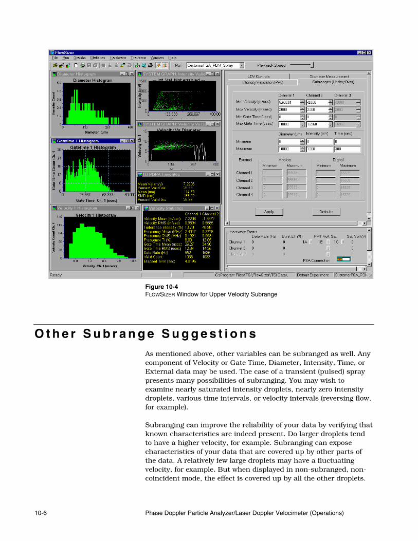
10-6 Phase Doppler Particle Analyzer/Laser Doppler Velocimeter (Operations)
Figure 10-4 FLOWSIZER Window for Upper Velocity Subrange
O t h e r S u b r a n g e S u g g e s t i o n s As mentioned above, other variables can be subranged as well. Any component of Velocity or Gate Time, Diameter, Intensity, Time, or External data may be used. The case of a transient (pulsed) spray presents many possibilities of subranging. You may wish to examine nearly saturated intensity droplets, nearly zero intensity droplets, various time intervals, or velocity intervals (reversing flow, for example). Subranging can improve the reliability of your data by verifying that known characteristics are indeed present. Do larger droplets tend to have a higher velocity, for example. Subranging can expose characteristics of your data that are covered up by other parts of the data. A relatively few large droplets may have a fluctuating velocity, for example. But when displayed in non-subranged, non-coincident mode, the effect is covered up by all the other droplets.

Using Subrange, Coincidence Modes and Even-Time Sampling 10-7
So the best solution is to explore your data using subranges and coincidence.
S o f t w a r e C o i n c i d e n c e M o d e
This mode of operation is used when two quantities (e.g., velocity components) need to be collected or sampled simultaneously. For example, the coincidence mode of operation is used to obtain Reynolds stress values, instantaneous velocity vector and velocity-size and other correlations. Simultaneous sampling or collection of two quantities is done when both the measurements are obtained within a preselected small time window. This window is generally referred to as the Coincidence Window. To set up the Coincidence window, go to the set of controls on the upper right corner of the main software window. Select the LDV Controls tab (Figure 10-5).

10-8 Phase Doppler Particle Analyzer/Laser Doppler Velocimeter (Operations)
Figure 10-5 Coincidence Window Setup
Coincidence Window Selection Gate Scale (%)—The Gate Scale controls how many gate widths the software looks forwards and backwards from the gate on one channel to find a gate on another channel. This value is set for each enabled channel and ranges from 0–1000%. A typical value is 250%. The Gate Scale is measured from the center of the burst gate on the corresponding channel. With a Gate Scale of 100%, for instance, the software will look half a gate forward and behind the center of the gate. This is essentially the same as hardware coincidence. Refer to “Run Setup → Processor Matrix” in Chapter 2 for details on hardware coincidence. The upper burst gates in Figure 10-6 would be coincident with a 100% gate scale on each channel. With a gate scale of 200%, FLOWSIZER lengthens each burst gate by 100% forward and 100% behind. The upper burst gate in Figure 10-6 would again be coincident at this gate scale. The lower burst gate would not be coincident at 100% or 200% gate scale but are coincident at 300% gate scale.

Using Subrange, Coincidence Modes and Even-Time Sampling 10-9
Coincidence Int. (µs)—This specifies a coincidence interval in microseconds. This value is added to each coincidence window. Thus, coincidence is determined by a combination of percent of gate time and a fixed window. Just one of the methods can be used by setting the other to zero. Coincidence interval becomes important with very short gate times because time stamp resolution limits the ability of particles to exhibit overlapping. In flows where the mean gate time is less than 2 µs, consider using a 1 µs Coincidence Interval. When the mean gate time is less than 1 µs, you should always use a Coincidence Interval of 1 µs to 2 µs.
Figure 10-6 Examples of Software Coincidence Checking
Software Coincidence Mode of Operation To activate Software Coincidence mode of operation go to the main software window.
Figure 10-7 Software Coincidence Button Press the button identified as Software Coincidence (Figure 10-7). This will activate Software Coincidence mode of operation.
When data are played back, you may notice more or less total samples present. This is normal and results from the fact that for software coincidence, no data is discarded, it is simply not shown. Thus, if the coincidence window is increased, you could possibly

10-10 Phase Doppler Particle Analyzer/Laser Doppler Velocimeter (Operations)
increase the Maximum Particle Measurement Attempts and obtain more total samples.
For a one-component PDPA system, Coincidence mode selection would result in using only data points that have both velocity and size information. In other words, data points with only velocity and no size measurements would not be displayed. For multi-component PDPA systems, Coincidence selection would result in using or selecting data points that have both size and the multiple components of velocity measurements. For size-velocity correlation results, the system needs to be operated in Coincidence mode.
In the case of three-component LDV systems, selecting coincidence would result in only using data points that have all three-component measurements. This means that all three velocity component measurements occurred within the specified Coincidence window time. The same comments are valid for a two-component LDV system. If the LDV or PDPA system is collecting external data (e.g., pressure), to calculate velocity-pressure or size-pressure correlations, the system needs to be operated in Coincidence mode.
Coincidence is also used with Subranging. Subranging sets bounds for the variables we are examining. Coincidence sorts out all the other data so that we are left with only those that are associated with data within the subrange.
No data is ever deleted or lost when using the subrange and/or coincidence features. It is simply not shown.
Software Coincidence Capture To this point, software coincidence has been discussed in terms of playing back saved data. When new data are acquired with software coincidence enabled, you will obtain the same number of samples on each channel enabled. Be aware that additional noncoincident data are also saved. As a result, the computer’s memory could be consumed by noncoincident samples and could cause capture to be terminated (in low coincidence situations). Hints
1. Optical overlap of the measurement volumes determines your coincidence ratio. Unreasonably long gate scales (>500%) cannot compensate for misaligned measurement volumes—including 3D probe layouts. It is advisable to use your microscope objective to verify overlap of the measurement volumes before you begin taking data. See the “TM/TR Series Fiberoptic Probe” manual for more details.

Using Subrange, Coincidence Modes and Even-Time Sampling 10-11
2. When using hardware coincidence with PDPA systems, you must use software coincidence as well, to ensure each diameter measurement also has a velocity measurement. Hardware coincidence only checks for internal overlap of the gates (in the FSA), not the presence of a valid diameter.
3. Typical Gate Scale settings are 250%. Typical Coincidence Interval settings are 1 or 2 µs and become necessary when mean gate times are less than 1 µs.
4. Good 3D coincidence starts with use of the pinhole and then the microscope objective, to achieve good overlap of measurement volumes. Then the FLOWSIZER Burst Monitor or an oscilloscope can be used to achieve the best overlap of channel 1/2 burst gates with channel 3 burst gates.
E v e n - T i m e S a m p l i n g LDV is a technique where the flow’s velocity is sampled, and particles crossing the measuring volume determine when samples are taken. Enabling Even-Time Sampling causes the software to not use all the possible samples, but only one sample out of a given time period. The main benefit of this approach is to remove velocity bias. Even-Time Sampling is not done in the processor, but in the FLOWSIZER software. The software selects one data point from each time interval using the data’s time stamp.
Velocity Bias The concept of velocity bias is easiest to explain in terms of mean velocity. By “mean” we are referring to a time average. In other words, the “mean” of a continuous but fluctuating analog signal is the value obtained with a sufficiently long averaging time so a second reading of the same flow would provide the same value within an acceptable error band.

10-12 Phase Doppler Particle Analyzer/Laser Doppler Velocimeter (Operations)
McLaughlin, et. al (1975
Figure 10-8 Velocity Bias In LDV, the measurement is on individual particles as they traverse the measurement volume. It is quite clear that as the velocity increases, more particles will traverse the measurement volume per unit of time. In fact the number should be proportional to the velocity. Therefore, if you simply average the individual measurements being made, the result will be biased to the high velocity side since there will be more measurements per unit of time at the higher velocities. As shown in Figure 10-8, in a one-dimensional flow situation, simply applying a correction based on the measured velocity works. But the flow is not normally one-dimensional. Also, any bias correction must consider all biases in the system, not just velocity. The best solution is to provide a high enough seed density so that uniform time sampling or some similar technique can be used.
Using the Even-Time Sampling Feature Even-Time Sampling is enabled under the LDV Controls tab on the upper right corner of the screen. Checking the enable box causes the software to use only one data point, the first point in time, from each time interval. Enter the time interval in microseconds. When selecting the time interval, the main thing to keep in mind is that the processor data rate must be several times larger than the even-time sampling data rate. The processor data rate is displayed in the hardware status box in the lower right corner of the screen. The even-time sampling rate is 1/sampling interval. The result of even-time sampling is that the samples obtained are at equally spaced

Using Subrange, Coincidence Modes and Even-Time Sampling 10-13
time intervals. The data arrival (due to particle arrival in the measuring volume) is random. In the even-time sampling process, the first available data point in each time interval is taken as the sample. Hence, the data rate needs to be much higher (say, about 10 times) than the sampling rate, so that the collected samples occur very close to the sampling time. Consequently, the minimum even-time sampling interval you can use will be determined by your processor data rate.


11-1
C H A P T E R 1 1 Outputting Analog Data
In some cases you may want to output an analog signal, which is proportional to the signal frequency (particle velocity) or phase (particle size) of the signal. This is a simple two-step process. First set up the software and second connect to the Analog Out BNC that is found on the back of the FSA processor. To set up the software go to Run → Run Setup. Then select the Processor/Matrix tab. You should now see a window similar to the one shown in Figure 11-1.
Figure 11-1 Window for Selecting what Analog Signal to Output

11-2 Phase Doppler Particle Analyzer/Laser Doppler Velocimeter (Operations)
Look at the Analog out portion of the window. Depending on how many channels of velocity you have enabled and whether or not you have sizing enabled, you will see certain parameters grayed out. In this example, the system is set up for two channels of velocity and size. Thus the Channel 3 Freq is grayed out. Select the parameter that you wish to output as an analog signal. You can only output one signal at a time. In this example, we are outputting the channel 1 frequency. Next connect a standard BNC cable to the BNC connection on the back of the FSA labeled Analog Out. This BNC output provides a 0- to 10-volt signal corresponding to the frequency or phase that you have selected. The output is updated for every valid burst from the selected parameter. When data capture is started from the software, the output resets to 0 volts until the first valid burst occurs. The range of frequencies indicated by the analog out voltage depends on the bandpass filter range selected in the FLOWSIZER software as shown in the following table. Note that this output indicates frequency, not velocity, so there may not be a 1 to 1 relation between the two depending on the type of downmixing used. If phase is selected, 0 volts corresponds to 0 degrees and 10 volts corresponds to 360 degrees. This output can supply up to 30 milliamps of current. Bandpass Filter Range
Frequency
Voltage
Frequency
Voltage
0.3–3 kHz 0.3 1 3 10
1–10 kHz 1 1 10 10
3–30 kHz 3 1 30 10
10–100 kHz 10 1 100 10
30–300 kHz 30 1 300 10
100–1000 kHz 100 1 1000 10
0.3–3 MHz 0.3 1 3 10
1–10 MHz 1 1 10 10
2–20 MHz 2 1 20 10
5–30 MHz 5 1 30 6
5–40 MHz 5 1 40 8
5–50 MHz 5 1 50 10
10–65 MHz 10 1 65 6.5
20–80 MHz 20 2 80 8
10–100 MHz 10 1 100 10
50–100 MHz 50 5 100 10
40–120* MHz 40 2 120 6
60–150* MHz 60 3 150 7.5
20–175* MHz 20 1 175 8.75
75–175* MHz 75 3.75 175 8.75
*FSA 4000 only

12-1
C H A P T E R 1 2 Using RMR (Shaft Encoder or OPR)
This chapter briefly covers the approach to input RMR—Shaft encoder or OPR (once-per-rev). The first screen is found under Run → Run Setup. Then select the RMR tab, as shown in Figure 12-1.
Figure 12-1 RMR Screen
12-2 Phase Doppler Particle Analyzer/Laser Doppler Velocimeter (Operations)
D e g r e e s P e r C y c l e
The resolver attaches a once-per-revolution pulse for every rotation (360 degrees) or every two rotations (720 degrees).
360 Select if the experiment test range is over a 360-degree cycle.
720 Select if the experiment test range is over a 720-degree cycle. To create a 720-degree period, every other “once-per-rev pulse” is ignored. Use the active real-time displays to make sure that the windows are synchronized with the right “once-per-rev pulse.”
D i r e c t i o n
The graphical RMR window selection control can be changed to make it easier to visualize the selected windows. This control reflects the direction selected.
CCLW Choose this to select counterclockwise direction. The displayed angles increase counterclockwise
CLW Choose this to select clockwise direction. The displayed angles increase in a clockwise direction.
E n c o d e r P a r a m e t e r s
Allows you to specify the following parameters:
Mode The following modes of operation are available.

Using RMR (Shaft Encoder or OPR) 12-3
RMR Off
This is the default selection and corresponds to a case when no RMR is used. Once Per Rev.
Choose this when the signal input into the RMR is the once-per-rev (OPR) signal. The RMR will use a once-per-rev pulse as a synchronizing input and divide the revolution period into 3600 pulses. This method relies on a stable time period between once-per-rev pulses. If the periods are not stable, the OPR Out Of Tolerance will flash and the data for that cycle will be marked as Out of Lock. Use the “Tolerance” to select the maximum fluctuation allowed to be considered in lock. Shaft Encoder x2
This mode multiplies the shaft encoder resolution by 2. For example, if the shaft encoder has a basic resolution of 500 then the Resolver Points Per Cycle value will be equal to 1000. Shaft Encoder x4
This mode multiplies the shaft encoder resolution by 4. For example, if the shaft encoder has a basic resolution of 500 then the Resolver Points Per Cycle value will be equal to 2000.
Tolerance (Degree) This selection determines how stable the once-per-rev pulse needs to be and still be considered in lock. The value needs to be expressed in degrees. This means that a nominal 3600 pulses per Revolution OPR with 1 degree selected can vary from 3610 to 3590 pulses per revolution and still be considered in lock.
Pulses Per Revolution The number of encoder points per revolution output by the shaft encoder installed on the system. If (operating) Mode: Once per rev. is selected, the only choice is the default value of 3600.
Disable Inhibit Windows The inhibit windows enable you to inhibit data collection at certain angular positions, such as when a rotating blade is in the
12-4 Phase Doppler Particle Analyzer/Laser Doppler Velocimeter (Operations)
measuring volume. Checking this box disables this feature and allows data collection at all angles. Unchecking this box causes data collection inhibiting to follow the windows you setup as defined below.
Reset Time Stamp at OPR This provides the option to reset the time stamp, if desired, when the once-per-revolution signal is received. This applies to once-per-revolution or shaft encoder mode.
Windows This set of parameters controls the creation and adjustment of acquisition windows. To update the RMR hardware to match the display, press the Apply button. RMR Windows Display Graphic
The screen contains a display control in the shape of a circle with the current selected windows displayed as pie-shaped wedges at the defined angles. The quadrant angles are marked in degrees based on direction. Each window is marked with its window number. If a window is selected, it will be drawn in a cross-hatch pattern. Max. Angle and Min. Angle provide the beginning and end of the window. Modifying RMR Windows
To modify windows follow these procedures:
Auto This selection brings up a set of controls to generate equally spaced windows. Automatic RMR Window Generation Parameters
The following describes the Automatic RMR Window Generation parameters.

Using RMR (Shaft Encoder or OPR) 12-5
Figure 12-2 Automatic RMR Window Generation Number of Windows
The number of windows desired per period. The windows are evenly divided into 360 (720 if selected) degrees. Size (degrees)
The size of each window in degrees. Offset Angle (degrees)
The offset that will be added to the placement of all of the windows. In effect the whole window pattern is shifted in degrees by this amount. Use the offset to adjust the window pattern. Abs Offset (degrees)
The amount by which the graphic display is shifted. Use this to adjust the display to match the actual model so that the “0” angle is at a more intuitive point rather than the default position.
OK Selects choices made.
Cancel Exits without saving any changes made. After using the Auto. Approach to select the window duration, each window width could be altered by typing in Min. and Max. Angle desired for the window.
Windows This information field displays the number of windows per cycle.

12-6 Phase Doppler Particle Analyzer/Laser Doppler Velocimeter (Operations)
Selected Displays the number of the selected window. This window is displayed in the graphic control in a cross-hatch pattern with minimum and maximum values displayed in the Max and Min boxes. To change the “Selected” window, type in the window you want to select in the entry field or left click on the window you want to select.
Max. Angle Edge of the selected window with the largest angle value.
Min. Angle Edge of the selected window with the smallest angle.
Post Processing RMR post processing enables you to view the mean and rms of diameter, volume, and velocity data binned by RMR angles. You can bin your data either by angle or by time interval. Apply
Sends the settings from the graphic control to the RMR hardware. Window settings do not become effective until this button is pressed.

13-1
C H A P T E R 1 3 Setting Up and Using a Traverse
If you are using a traverse in your experiment, you need to set up the mode in which you want to operate it and also set the parameters through the Traverse menu option.
Select Traverse → Start to open the main traverse interface.
Select Traverse → Scan Capture to start the automatic capture process based on the Matrix of positions and filenames you selected. Matrix can be entered manually or automatically. The spreadsheet within this module is fully compatible with Microsoft® Excel. Therefore, you can copy and paste to and from both applications. Please refer to “Sweep Capture” section in Chapter 3 to capture data while traverse is moving.
S e t t i n g t h e T r a v e r s e P a r a m e t e r s To specify the traverse parameters, select the Traverse option from the command menu bar and then select one of the three control options:
Manual
Auto
Matrix
The following paragraphs describe these parameters.

13-2 Phase Doppler Particle Analyzer/Laser Doppler Velocimeter (Operations)
Figure 13-1 Traverse Manager Screen
Manual This option allows manual control of the traverse. The following parameters or options are available: Manual Setup
Parameter Description Stop
Halts traverse motion. Motion on the x, y, z, u, v, and w axes stops and the current position of the traverse is read and displayed in the X, Y, Z, U, V, and W group boxes.
Move To
Moves all connected axes to the position entered in the X, Y, Z, U, V, W, Move boxes.
Jog+
Moves all connected axes by the displacement value entered in the X, Y, Z, U, V, W, Jog boxes in the positive direction.
Jog-
Moves all connected axes by the displacement value entered in the X, Y, Z, U, V, W, Jog boxes in the negative direction.

Setting Up and Using a Traverse 13-3
Parameter Description X, Y, Z
• The X, Y, Z, group boxes do the following: The top lines in each box show the current positions of the x, y, and z axes of the traverse.
• The boxes next to the Move button allow you to enter a new position for each axis. When you press the Move button, all three axes of the traverse move to this new position.
• The boxes next to the Jog button allow you to enter a displacement value by which you can move all three axes of the traverse. For example, if you specify .1 in the Jog boxes, when you hit Jog, all three axes move by .1.
• The + or - buttons next to the displacement value boxes allow you to individually move, each axis of the traverse—plus or minus the selected displacement value.
More Displays three more axis U, V, W.
Local
Releases the traverse control from the computer to a hardware hand control (joystick).
Remote Restores computer control of the selected traverse.
Abs Home Moves the traverse to its hardware zero reference point. This puts the traverse at a known reference location, indicated as 0,0,0. All future indicated positions are displacements from this point.
Rel Home Moves the traverse to its relative zero position using the “Set Rel 0” command.
Set Rel 0 Assigns the current traverse position as the 0,0,0 reference point. All future indicated positions are displacements from this point. Current position will be set to display 0,0,0.
Setup Set up all the driver settings, communication settings, and axis settings.

13-4 Phase Doppler Particle Analyzer/Laser Doppler Velocimeter (Operations)
Figure 13-2 Communication Setup Dialog Screen Communication Setup
Parameter Description Manual Move Move the traverse by yourself. There will be no
driver and communications needed.
Driver Select which traverse driver to use.
Comm Port Set the serial port the traverse is connected to.
Baud Rate RS-232 setting determined by your traverse controller.
Data Bits RS-232 setting determined by your traverse controller.
Parity RS-232 setting determined by your traverse controller.
Stop Bits RS-232 setting determined by your traverse controller.
Flow Control RS-232 setting determined by your traverse controller.

Setting Up and Using a Traverse 13-5
Figure 13-3 Axis Setup Dialog Screen Axis Setup
Parameter Description Axis Select which axis to set up.
Axis Enabled Enable/Disable this axis.
Title Name of this axis.
Units Units of this axis, e.g., mm or inch
Digits How many decimal points to use.
Max Travel Steps Specify the maximum number of step the traverse can travel along each axis.
Time Out (s) Set the timeout limit of the axis.
Velocity (steps) Velocity of the axis, -1 means not supported.
Acceleration (steps) Acceleration of the axis, -1 means not supported.
Wait Time In Pos. (s) Wait time in seconds after traverse moves to specified position before data capture starts.
Relative Home Enabled: Enable/Disable relative home. Your traverse controller should give its feedback to this setting. Absolute Position: Absolute position of the relative home of this traverse.

13-6 Phase Doppler Particle Analyzer/Laser Doppler Velocimeter (Operations)
Auto This selection moves the traverse step-by-step along the path stored in the current traverse position list. Use this option to test or pre-run the traverse position list for any problems before making an actual acquisition run. You can also use this option to determine if, and where, instrument commands need to be added to a position file. The current position list is displayed at the bottom of the dialog box. To select a different position list, select Matrix → Open to open an existing traverse file.
Figure 13-4 Auto Dialog Screen

Setting Up and Using a Traverse 13-7
Auto Setup
Parameter Description Previous Moves the traverse backwards one position.
Each press of this button moves the traverse to the previous position, sends out any embedded commands, and updates the position displays. Use the Matrix control to edit traverse position or commands.
Next Moves the traverse forward one position. Each press of this button moves the traverse to the next position, sends out any embedded commands, and updates the position displays. Use the Matrix control to edit traverse position or commands.
Current Position X: Current entry of X axis in the Matrix. Y: Current entry of Y axis in the Matrix. Z: Current entry of Z axis in the Matrix. U: Current entry of U axis in the Matrix. V: Current entry of V axis in the Matrix. W: Current entry of W axis in the Matrix. Run Setup: Current entry of Run Setup in the Matrix. Save As: Current entry of Save As in the Matrix.
Matrix This option provides you with a spreadsheet that can be used to create and maintain traverse position lists. Traverse position lists can contain, besides position information, embedded Run Setup files and Save As files. This allows you to optimize the settings for these instruments for each position in a list without relying on a general setting for all cases.

13-8 Phase Doppler Particle Analyzer/Laser Doppler Velocimeter (Operations)
Figure 13-5 Matrix Dialog Screen Parameter Description
The traverse position list is displayed in the spreadsheet in columns. The following describes the contents of each of these columns.
Parameter Description X Contains X position.
Y Contains Y position.
Z Contains Z position.
U Contains U position.
V Contains V position.
W Contains W position.
Run Setup Name of the Setup file for this position. During scan capture, FLOWSIZER software will load this setup file and take data based on all the settings stored in the file.
Save As Name of the Save As file for this position. During scan capture, FLOWSIZER software will save captured data to this file automatically.
Open Open an existing .trv traverse file.
Apply Apply all the matrix information to the software.
Save Save current matrix to a .trv traverse file.
Save As Save current matrix to a different .trv traverse file.

Setting Up and Using a Traverse 13-9
Editing Commands
The right mouse button brings up the following pop-up menu of specific traverse file editing commands.
Figure 13-6 Auto Fill-Column Screen
Command Description Insert Row Adds a new line at the cursor position. Use in create
space for an embedded command in the traverse position list.
Delete Row Deletes the line at the cursor position.
Auto Axes: Select the axis to do auto fill. Start Row: Start row number. End Row: End row number. Starting Number: Start value. Scale: Linear increase linearly, while Log increase logarithmically.
Cut Cuts highlighted text.
Copy Copies cut text to the clipboard.
C r e a t i n g a S i m p l e T r a v e r s e P o s i t i o n L i s t This list starts at position 0,0,0 and moves in the positive x, y, and z directions ten positions, 1-mm per position. This example uses a linear relation to do the automatic position generation.
1. From the Matrix page, click the left mouse button to bring up the Edit menu.
2. From the Edit menu option, select Insert Row. This inserts a new row into current spreadsheet.

13-10 Phase Doppler Particle Analyzer/Laser Doppler Velocimeter (Operations)
3. Repeat step 2 ten times to create ten rows.
4. Enter 0 in the first row of columns X, Y, Z. This will be the initial position.
5. Click the left mouse button to bring up the Edit menu, select Auto Fill option.
6. In the Auto Fill dialog box, select X axis, enter 1 in the start row, enter 10 in the end row, enter 0 in the starting number, enter 1 in increment, and select Apply.
7. Make similar steps for the other two axes.
8. Enter a Run Setup filename in the uppermost Run Setup box.
You only need to enter the name to the first position that has a setup file change, the software will fill the rest automatically once you click the Apply button.
9. Enter a filename in the Save As box. The software will generate the rest automatically once you click the Apply button.

14-1
C H A P T E R 1 4 Using the Burst Monitor
The capabilities of FLOWSIZERTM Data Acquisition and Analysis
Software to display acquired data are very powerful and versatile. But in addition to that, FLOWSIZER also has the capability to display the actual Doppler bursts as they are being processed! This feature is useful in optimizing your settings to improve the data rate, validation rate, and data reliability. It is also useful in troubleshooting, when a good digital oscilloscope is not available. Select Hardware → Burst Monitor to open the Burst Monitor Window. Figure 14-1 shows the Burst Monitor Window. First select the channel you wish to display. For PDPA systems, select channel 1 and the channel 1A, 1B and 1C signals will be displayed. An LDV system will display only individual channels. Then select either Continuous or Single Read to continuously monitor the burst stream, or, capture single “snapshots” of the burst stream. The burst monitor shows the signal after downmixing and bandpass filterings as it appears when being sampled, or digitized. This is the same signal seen on the signal out BNCs on the FSA front panel. In fact, the amplitude, into 50 ohms, at this connector corresponds to the amplitude shown in the burst monitor. The main use of this monitor is to check the quality of the burst signals being processed, specifically their amplitude and noise level. The PMT voltage should be high enough so that some of the signals are close to ±.5 volts in amplitude, which is the full scale of the 8-bit A/D converters. Having some very large signals peg, or max out the A/D full scale is not a problem and even desirable so that the smaller particles have enough gain. Noisy signals don’t have a clean looking sinewave and also have only a few samples. Good quality signals will have a large proportion of the bursts with the maximum number of samples, 256. The portion of the signal shown is not the whole burst, but only the center portion used by the burst processing DSPs to calculate frequency + phase. The 10–1 bandpass filter ranges are further divided into three subranges to optimize samples/cycle. The subrange is indicated by showing time scale x1, x2, or x4. If the time scale is x2, the frequency displayed is actually ½ of the x1 range. If it is x4, the frequency is ¼ of the x1 range. Note also that the FSA’s maximum data rate is lower when the burst monitor

14-2 Phase Doppler Particle Analyzer/Laser Doppler Velocimeter (Operations)
window is open, because the FSA is busy transferring raw data to the computer.
Figure 14-1 Burst Monitor Window

15-1
C H A P T E R 1 5 Exporting Data in ASCII Format
To export your data go to File → Export Data. A dialog box like the one shown in Figure 15-1 should open.
Figure 15-1 Export Data Dialog Box You can then choose which parameters you would like to export. To select parameters for export simply click on the parameter you would like to export and then click the > button. (To remove a parameter that you already selected, click the < button.) When you

15-2 Phase Doppler Particle Analyzer/Laser Doppler Velocimeter (Operations)
have chosen all the parameters you want to export, click the Export button. A text file will then be created and stored in the location shown in the Export File edit box.
E x p o r t F o r m a t This allows you to choose the format of your export files. Both of them are text files. .csv files can be loaded directly into Microsoft Excel, .dat can be loaded directly into TecPlot.
E x p o r t H e a d i n g s ( f i r s t r o w ) If this check box is selected, the first row of the exported file will contain which parameters you have chosen (along with the units) and the order they were exported in.
E x p o r t t o 1 F i l e Checking this box allows you to export the data from multiple FLOWSIZER runs into one *.csv file. If you only have one run selected and you check this box, it will just export that one run into the *.csv file. If this box is unchecked, the Export File edit box will be grayed out and the current run you are processing will be saved with the same name and in the same folder as the data file you are processing. If this box is checked, you can select where to save the resulting *.csv file by clicking on the … button which is to the right of the Export File edit box. To select multiple FLOWSIZER runs to process into one *.csv file, you must select all the runs you want to process by going to File → Experiment Manager, and selecting the runs you want to process (use the Ctrl key to select more than one run). Then open the Export File Dialog Box, make sure the Export to 1 file edit box is checked, and select a location and name for the resulting *.csv file. Then export the data and the data from all the runs will be put in one *.csv file.

Exporting Data in ASCII Format 15-3
A p p l y C u r r e n t S e t t i n g s t o A l l R u n s This box applies only when you are exporting multiple FLOWSIZER runs into one *.csv file. By checking this box the settings from the very first run will be applied to all selected runs when creating the *.csv file. It is probably not likely to be used very often.
When you are done exporting the data, click on the Done button to close the Export File Dialog Box. The set of parameters that you last exported will be saved, so the next time you choose to export data, these parameters will automatically be selected when the Export File Dialog Box is opened.


16-1
C H A P T E R 1 6 Matrix Transformation
M a t r i x T r a n s f o r m a t i o n P a g e In two- and three-component LDV/PDPA systems, the measured velocity directions do not always coincide with the desired world coordinate system. The FLOWSIZER
TM Data Acquisition and Analysis Software can transform the measured non-orthogonal velocity (V1, V2, V3) to the orthogonal velocity components (u, v, w) in the world coordinate system (x, y, z). To perform this transformation, you need to setup a transformation matrix in the FLOWSIZER software.
What is Transformation Matrix? The transformation matrix can be derived from the projection of the orthogonal velocity (u, v, w) along the measurement directions
),,( 321 eeeek =r:
⎥⎥⎥
⎦
⎤
⎢⎢⎢
⎣
⎡⋅
⎥⎥⎥
⎦
⎤
⎢⎢⎢
⎣
⎡=
⎥⎥⎥
⎦
⎤
⎢⎢⎢
⎣
⎡⋅=
⎥⎥⎥
⎦
⎤
⎢⎢⎢
⎣
⎡
wvu
eeeeeeeee
wvu
EVVV
zyx
zyx
zyx
333
222
111
3
2
1
The inverse of projection matrix E is the final transformation matrix that is used to convert the non-orthogonal velocity components (V1, V2, V3) to the orthogonal velocity (u, v, w). In the next section, you can find the projection matrix E for some typical LDV measurement configurations. Since the FLOWSIZER software automatically calculates the inverse of matrix E to get the transformation matrix, what you need to enter in the software is simply the projection matrix E itself.
Examples of Projection Matrix Case 1. Three-Component Measurement Using Two Probes in the Same Plane
Figure 16-1 shows the typical setup of two-probe measurements, in which probe A has a two-component transmitter and both probes

16-2 Phase Doppler Particle Analyzer/Laser Doppler Velocimeter (Operations)
are in the YZ plane. The projections of orthogonal velocity components (u, v, w) onto the measurement directions are:
ββαα
sincossincos
3
2
1
wvVwvV
uV
+⋅−=−⋅−=
=
where V1 and V2 are measured by probe A, and V3 by probe B. α and β is the angle between the axis z and the optical axis of probe A and probe B, respectively. γ is the angle between the optical axis of probe A and the YZ plane. α, β and γ are defined between 0 and 90 degrees. The projection matrix E to be entered in the FLOWSIZER software, for the world coordinate system shown in Figure 16-1, is given below,
x y z 1 1 0 0 2 0 - cosα -sinα 3 0 -cosβ sinβ
If the world coordinate system is different from that shown in Figure 16-1, the sign of eij in the projection matrix is determined by the angle between the measurement direction Vi and the axis xj: eij is positive if the angle is less than 90 degrees, and negative if the angle is between 90 and 180 degrees.
A B
Unshifted beam
Shifted beam
αβ
A B
V2
V3 Y
Z
Top view
A B
Unshifted beam
Shifted beam
αβ
A B
V2
V3 Y
Z
Top view
Figure 16-1 Three-Component Velocity Measurement Using Two Probes in the Same Plane

Matrix Transformation 16-3
Case 2. Three-Component Measurement Using Two Probes not in the Same Plane
Figure 16-2 shows the setup of two-probe measurement similar to that shown in Figure 16-1 except that probe A is not in the YZ plane. The projections of orthogonal velocity components (u, v, w) onto the measurement directions are:
ββαα
γαγαγ
sincossincos
sincossinsincos
3
2
1
wvVwvV
wvuV
+⋅−=−⋅−=
⋅+⋅⋅−⋅=
where V1 and V2 are measured by probe A, and V3 by probe B. α and β is the angle between the axis z and the optical axis of probe A and probe B, respectively. γ is the angle between the optical axis of probe A and the YZ plane. α, β and γ are defined between 0 and 90 degrees. The projection matrix E to be entered in the FLOWSIZER software, for the world coordinate system shown in Figure 16-2, is given below:
x y z 1 cosγ -sinα⋅sinγ cosα⋅sinγ 2 0 - cosα -sinα 3 0 -cosβ sinβ

16-4 Phase Doppler Particle Analyzer/Laser Doppler Velocimeter (Operations)
X
A Projection of A’s optical axis in YZ plane
γV1
A B
αβ
A B
V2
V3 Y
Z
AA
View AA
Top view
Unshifted beam
Shifted beam
X
A Projection of A’s optical axis in YZ plane
γV1
A B
αβ
A B
V2
V3 Y
Z
AA
View AA
Top view
Unshifted beam
Shifted beam
Figure 16-2 Three-Component Velocity Measurement Using Two Probes not in the Same Plane If the world coordinate system is different from that shown in Figure 16-2, the sign of eij in the projection matrix is determined by the angle between the measurement direction Vi and the axis xj: eij is positive if the angle is less than 90 degrees, and negative if the angle is between 90 and 180 degrees, except for the two special cases given below:
a. e1y is positive if the angle between the probe A’s projection in YZ plane and the measurement direction V1 AND the angle between the projection and the axis y are BOTH less than or BOTH greater than 90 degrees;
b. e1z is positive if the angle between the probe A’s projection in YZ plane and the measurement direction V1 AND the angle between the projection and the axis z are BOTH less than or BOTH greater than 90 degrees..

Matrix Transformation 16-5
Case 3. Three-Component Measurement Using One 5-Beam Probe
Figure 16-3 shows the typical setup of 5-beam probe measurement, in which three velocity components are measured by a single three-component transceiver probe. The projections of orthogonal velocity components (u, v, w) onto the measurement directions are:
ββγγαα
sincossincossincos
3
2
1
wuVwvVwuV
−⋅=+⋅=
⋅+⋅=
where V1 is measured by green beam, V2 by blue beam, and V3 by violet beam. α and β is the angle between the Z axis and the optical axis of the green and violet beam pairs, respectively. γ is the angle between the optical axis of the 5-beam probe and the axis z. α, β and γ are defined between 0 and 90 degrees. The projection matrix E to be entered in the FLOWSIZER software, for the world coordinate system shown in Figure 16-3, is given below,
x y z 1 cosα 0 sinα 2 0 cosγ sinγ 3 cosβ 0 -sinβ
If the world coordinate system is different from that shown in Figure 16-3, the sign of eij in the projection matrix is determined by the angle between the measurement direction Vi and the axis xj: eij is positive if the angle is less than 90 degrees, and negative if the angle is between 90 and 180 degrees. A special case of 5-beam probe measurements is when γ = 0; i.e., the optical axis of the probe is perpendicular to the Y axis.

16-6 Phase Doppler Particle Analyzer/Laser Doppler Velocimeter (Operations)
Y
Z γV2
α
β
V1 V3
X
Z
Unshifted beam
Shifted beam
Side view
Top view
Y
Z γV2
α
β
V1 V3
X
Z
Unshifted beam
Shifted beam
Side view
Top view
Figure 16-3 Three-Component Velocity Measurement Using a 5-Beam Probe Case 4. Two-Component Measurement Using One Probe
Figure 16-4 shows the setup of single-probe measurement of two velocity components. Normally no transformation is needed for this case since the two measurement directions are orthogonal. However, sometimes the world coordinate system is rotated (along the axis z) from the measurement coordinate system (as seen in the end view in Figure 16-4), and an affine transform is needed to obtain the velocity components (u, v, w) in the world coordinate system. The projections of orthogonal velocity components (u, v, w) onto the measurement directions are:
αααα
cossinsincos
2
1
vuVvuV
+⋅=−⋅=
where α is the angle from the axis x to the measurement direction V1 and is defined between -180 degrees to 180 degrees with clockwise direction being the positive.
The projection matrix E to be entered in the FLOWSIZER software is given below. Please note that the signs of the elements in this matrix are fixed and the angle α can be negative values.

Matrix Transformation 16-7
x y z 1 cosα -sinα 0 2 sinα cosα 0 3 0 0 1
α V2V1
Y
X
Unshifted beam
Shifted beam
YZ
Top view End view
α V2V1
Y
X
Unshifted beam
Shifted beam
YZ
Top view End view
Figure 16-4 Two-Component Velocity Measurement Using One Probe Case 5. Two-Component Near-Wall Measurement Using a Probe with Prism
Figure 16-5 shows the setup of near-wall velocity measurement using a probe with two-beam transmitter. A prism is used to move the bottom beam to the center to facilitate near-wall measurement. The projections of orthogonal velocity components (u, v, w) onto the measurement directions are:
vVwuV
=⋅+⋅=
2
1 sincos γγ
where the angle γ is determined by the green beam separation and the focal length of the probe. Since the angle γ is very small, the measurement direction V1 is almost aligned with the axis x and the contribution from velocity component w to V1 can be neglected. The projection matrix E to be entered in the FLOWSIZER software, for the world coordinate system shown in Figure 16-5, is given below,
x y z 1 cosγ 0 0 2 0 1 0 3 0 0 1
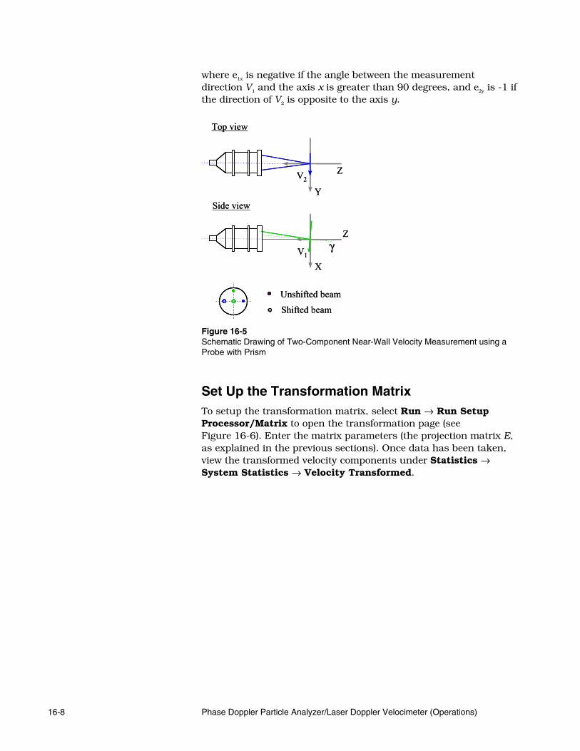
16-8 Phase Doppler Particle Analyzer/Laser Doppler Velocimeter (Operations)
where e1x is negative if the angle between the measurement direction V1 and the axis x is greater than 90 degrees, and e2y is -1 if the direction of V2 is opposite to the axis y.
V2Z
Y
V1
Z
X
γ
Top view
Unshifted beam
Shifted beam
Side view
V2Z
Y
V1
Z
X
γ
Top view
Unshifted beam
Shifted beam
Side view
Figure 16-5 Schematic Drawing of Two-Component Near-Wall Velocity Measurement using a Probe with Prism
Set Up the Transformation Matrix To setup the transformation matrix, select Run → Run Setup Processor/Matrix to open the transformation page (see Figure 16-6). Enter the matrix parameters (the projection matrix E, as explained in the previous sections). Once data has been taken, view the transformed velocity components under Statistics → System Statistics → Velocity Transformed.
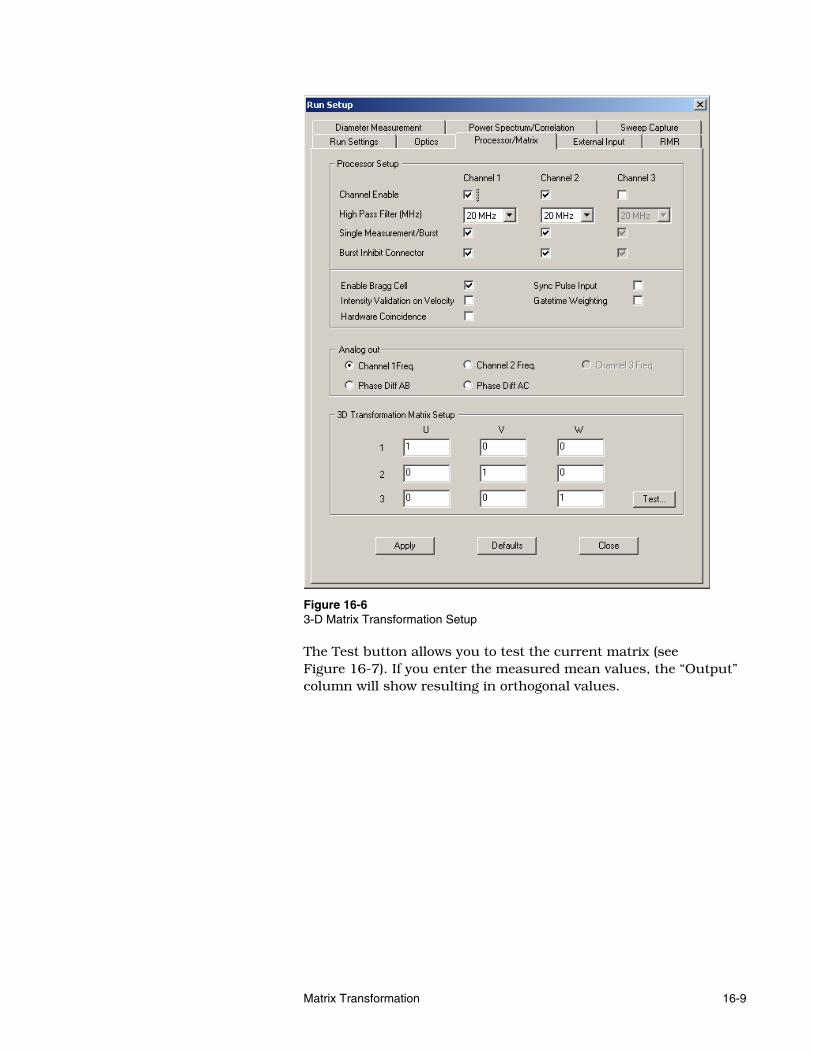
Matrix Transformation 16-9
Figure 16-6 3-D Matrix Transformation Setup
The Test button allows you to test the current matrix (see Figure 16-7). If you enter the measured mean values, the “Output” column will show resulting in orthogonal values.

16-10 Phase Doppler Particle Analyzer/Laser Doppler Velocimeter (Operations)
Figure 16-7 3-D Matrix Transformation Test

A-1
A P P E N D I X A Laser Doppler Velocimetry (LDV) Overview
The Laser Doppler Velocimetry (LDV) measurement technique uses a laser to generate a coherent (fixed frequency) beam to illuminate a moving particle in the flow. This particle movement creates a Doppler shift in the light frequency directly proportional to its velocity. Thus the measurement of such Doppler shift frequency is a measurement of the particle’s velocity. Since the particle is very small, one can be quite certain that the particle velocity is very close to that of the fluid velocity. By not inserting any sensor into the flow, this technique provides a noncontact way of measuring velocity.
Figure A-1 LDV Technique

A-2 Phase Doppler Particle Analyzer/Laser Doppler Velocimeter (Operations)
Some of the key aspects of this noncontact flow measuring technique are:
Measurement is, generally, independent of the property of the medium
Desired component of velocity can be measured by suitably orienting the laser beams
The signal exists only when a detectable particle is in the measurement volume and, hence, is discontinuous.
C o m p o n e n t s o f a n L D V S y s t e m The components of an LDV system are:
Laser—Monochromatic light source, provides coherent, collimated beam
Transmitting optics
Receiving Optics, Detector
Signal processor, Data Analysis system The dual-beam approach is the most common optical arrangement. Figure A-2 shows the basic components of a complete LDV system for velocity measurements.
Particles Movingwith the Fluid
Photodetector
SignalProcessor
No probe in the flowNo velocity calibrationDesired velocity components measured directly
Small measuring volumeLarge dynamic rangeHigh frequency response
Figure A-2 Dual-Beam Laser Anemometer

Laser Doppler Velocimetry (LDV) Overview A-3
O p t i m i z i n g L D V M e a s u r e m e n t s To optimize a measurement, you must have:
Particles that follow the flow and provide an adequate signal.
Laser, optics, and photodetector that provide a signal with optimum signal-to-noise ratio at the photodetector output.
A signal processor that extracts the maximum amount of information from the photodiode signal.
Data processing techniques that provide the needed flow properties from the output of the signal processor.
In many flows, if all these criteria are handled properly, very good data can be obtained that is simply not available by any other technique.
L a s e r S o u r c e Typically, an argon-ion laser is used as the laser source. This laser output has multiple wavelengths. The three wavelengths used for LDV/PDPA applications are 514.5 nm (green), 488.0 nm (blue), and 476.5 nm (violet).
D o p p l e r F r e q u e n c y M e a s u r e m e n t The Doppler shift frequency created by a moving particle is typically from a few kHz to more than 100 MHz, but is contained in its light frequency which is typically around 440 GHz. If we use two laser beams, each to create a Doppler effect on the moving particle, and mix the scattered light from the particle at the photodiode, the basic light frequency is subtracted, only the Doppler shift frequency which is much lower, is detected. In a one-channel LDV/PDPA system, two beams of equal intensity are generated. The two beams are then focused and crossed at an angle (half angle = κ) at the focal length of the lens. When a small particle in the fluid flows past the beam crossing, its scattered light is collected and focused onto a photodetector, creating the (Doppler) signal for velocity measurement. Scattered light from particles outside of the crossing point fall outside of the photodetector and do not get measured.

A-4 Phase Doppler Particle Analyzer/Laser Doppler Velocimeter (Operations)
F r i n g e S p a c i n g At the crossing point of the two beams, an interference fringe pattern is actually created by the coherence of the laser light source. This fringe pattern provides the necessary light pattern to illuminate the particles and is often used as an alternate method to explain the creation of the Doppler frequency signal (Figure A-3). The fringe spacing, (df) in an LDV system, depends only on the wavelength of light, (λ), and half angle, (k). The amplitude variation of the signal reflects the Gaussian intensity distribution across the laser beam. Collection (receiving) optics for the dual-beam system can be placed at any angle. The resulting signal from the receiving system still gives same frequency. However, signal quality and intensity varies greatly with angle.
u − flow velocity
λ − wavelength of incident light
fd − frequency detected at photodetector
f − focal length of the transmitting lens
κ
Laser
f
d
u
f
y fd d f
=
=
λκ2 sin
d f
uyu
Figure A-3 Fringe Descriptions
M e a s u r e m e n t V o l u m e D i m e n s i o n s The measurement volume is the body bound by the ellipsoidal surface shown in Figure A-4, and it corresponds to the surface on which the light intensity of the fringes is 1/e2 of the maximum intensity, which occurs at the center of the measurement volume. Fringe spacing decreases with increasing angle κ.

Laser Doppler Velocimetry (LDV) Overview A-5
NFR = number of fringes
V = volume of measurement volume
df = fringe spacing
dm = diameter of the measurement volume
lm = length of the measurement volume
f= focal length of the lens
λ= laser wavelength
d f D
d d
l d
V d Ndd
dD
e e
m e
m e
e FR
m
f e
− −
−
−
−
−
=
=
=
= = =
2 2
2
2
2
2
4
6 1273 2
λ π
κ
κ
π κ κ
/
/ cos
/ sin
/ ( cos sin ) .
2 κ
s 1
s 2
d
De -2
De - 2
zx
y
s 1
s 2 κ
κ
z
x
e -2 Contour
d mFringes
l m
df
df
d f ×= 5~~sin2
SpacingFringe
λκ
λ
Figure A-4 Measurement Volume Dimensions
D o p p l e r S i g n a l The light scattered by a particle passing through the fringes in the measurement volume is optically collected and focused onto the photomultiplier tube (PMT). The PMT produces an electrical current proportional to this light flux. Variations in this electrical current caused by the particle passing the fringes are subsequently analyzed to determine the velocity of the particle.
The signal output from the PMT can, typically, be decomposed to the following components:
Low frequency "pedestal" caused by the particle passing through the focused Gaussian-intensity laser beams.
d
f.~
d
f~
sind f ×= 50
2λ
κλ
κ
κ
πλ
sin/dl
cos/dd
D/fd
em
em
ee
2
2
22 4
−
−
−−
=
=
=
2
2
271 6 23
−− ===
ef
mFRe D
d.
d
dN)sincos/(dV κκπ

A-6 Phase Doppler Particle Analyzer/Laser Doppler Velocimeter (Operations)
Doppler frequency, fd, signal that is superimposed on the pedestal and has a regular sinusoidal pattern related to how fast the particle crosses the fringes in the measurement volume.
Wide bandwidth electronic noise generated by stray light, the PMT, and associated electronics.
Signal (a) in Figure A-5 is the sum of the pedestal component, the Doppler component and the noise from the photodiode. Since the pedestal is undesirable for good signal processing, it is usually removed by simply filtering the signal through a high-pass filter. The resulting signal, with pedestal-removed, is shown in (b). High frequency noise can be reduced by low-pass filtering the noise at a frequency which must be greater than fD in order to avoid filtering the Doppler signal. The low-pass filtered signal is shown in (c).
Figure A-5 Doppler Signal
L D V S i g n a l C h a r a c t e r i s t i c s Figure A-6 represents the variations in intensity distribution at the intersection region of two Gaussian beams. These would represent the output of a photodetector as a single particle passes along the indicated paths if:
The beams are polarized normal to the plane of the beams
The light scattered by the particle from two incident beams mixes to give 100 percent modulation depth on the photodetector output.

Laser Doppler Velocimetry (LDV) Overview A-7
The scattered light intensity is sufficient to give an essentially continuous signal.
Figure A-6 Signal Characteristics Along the Measurement Volume A particle that is small compared with the fringe spacing, df , normally produces a scattered light signal proportional to the light intensity incident on the particle. Under these conditions, the Doppler component of the signal, for example, the sinusoidal oscillating component, always has a Gaussian envelope, even though the sum of the Doppler component and the pedestals change shape substantially for various particle trajectories.
V a r i a t i o n o f S c a t t e r e d L i g h t I n t e n s i t y Figure A-7 shows the variation of the scattered light intensity as a function of receiver position for polarization perpendicular to the beams. The intensity values are obtained from the Mie scattering calculations. For a dual-beam system, the component of velocity measured is independent of the location of the scattered light collection system. The backscatter mode is a very convenient arrangement since all the optics are on one side of the measuring point, requiring only one window and providing easier traversing arrangement of the LDV system. In this case, the same lens is used for focusing the two beams and for collecting and collimating the scattered light.

A-8 Phase Doppler Particle Analyzer/Laser Doppler Velocimeter (Operations)
transmitter receiver receiver
receiver
receiverΦ
Φ = 180backscatter
Φ = 0forward scatter
off-axisforward scatter
off-axisbackscatter
Off-AxisBackscatter Off-Axis
Forward Scatter
Backscatter Forward Scatter
BackscatterForward ScatterReceiver Orientation Φ
Sca
ttere
d Li
ght I
nten
sity
, Rel
ativ
e U
nits Mie Scattering Theory
Polystyrene Latex ParticleFluid = WaterDiameter = 0.5 µmλ = 0.5145 µm
Figure A-7 Scattered Light Intensity Variation If direct backscatter is not used, then a separate receiving system, appropriately positioned to collect the scattered light, is used. Once the receiving optics is separate from the transmitting optics, the direct forward-scatter arrangement provides the strongest signal. In practice, to avoid reflections, an off-axis forward-scatter location for the receiver is often preferred.
T y p i c a l F r e q u e n c y v e r s u s V e l o c i t y C u r v e s
Figure A-8 shows the frequency versus velocity for two values of half-angle (k) between the two beams. Figure A-3 has the equation showing the relationship between frequency and velocity. Generally, velocity dynamic range of over 108 is achieved by LDV systems and for most common flows, the corresponding Doppler frequencies are in the kHz to MHz range.

Laser Doppler Velocimetry (LDV) Overview A-9
1.00E+00
1.00E+02
1.00E+04
1.00E+06
1.00E+08
1.00E+10
1.00E-06 1.00E-04 1.00E-02 1.00E+00 1.00E+02 1.00E+04
Velocity (m/sec)
Freq
uenc
y, H
z
λ = 514.5 nm
κ = 140
κ = 0.140
Figure A-8 Typical Frequency versus Velocity Curves The value of k = 14° represents a lens with an F-number (focal length/diameter) of 2. At k = 0.14°, the F-number would be about 200. These are reasonable limits using a single-focusing lens. The absolute minimum fringe spacing, df , is the laser wavelength divided by 2 (that is when sin k = 1, k = 90°). This gives frequencies of about 4 MHz per m/s of velocity for visible wavelength lasers (λ = 0.5). Velocity measurements from 1 µm/sec to over 1,000 m/sec which corresponds to a dynamic range of over 109, have been made with LDV.
F r e q u e n c y S h i f t i n g The purpose of frequency shifting in LDV is to:
Measure flow reversal.
Measure small fluctuations of velocity (in the presence of a large average velocity).
Extend the range of low and high velocities that can be measured by a processor.
Measure flow velocities in highly turbulent flows.
Figure A-9 shows the linear relationship between velocity and Doppler frequency fd. For the case of no frequency shift, the frequency of the Doppler signal (photodiode output) goes to zero as the velocity goes to zero and remains positive when the velocity becomes negative. Further, the Doppler signals generated by two

A-10 Phase Doppler Particle Analyzer/Laser Doppler Velocimeter (Operations)
particles, A and B, having equal velocity magnitude but opposite direction (one positive and other negative) will have the same frequency value fAB. From a fringe model standpoint, the fringes are stationary in a system with no frequency shift.
Velocity (+ ve)0Velocity (-ve)
Frequency
fringe motion
frequencyshift = f1
freq. shift =
f 1
freq. shift =
0freq. shift = 0
stationary fringes
stationary fringes
Α
Β
fA
fB
fAB
FringeMotion
Stationary Fringes
Stationary Fringes
Frequency
Velocity (-ve) Velocity (+ve)
Figure A-9 Frequency Shifting A system with frequency shift effectively offsets the frequency velocity curve along the y-axis by the frequency shift value. In Figure A-9, the frequency-velocity curve for a system with a frequency shift value of f1 is shown. For this system, a particle with zero velocity generates a signal of frequency f1. And as the velocity decreases, the frequency of the signal will be less than f1. The two particles A and B generate signals with frequencies fA and fB, respectively. From a fringe model standpoint, the system with frequency shift corresponds to a case where the fringes are moving. In Figure A-9, the fringe motion is opposite the velocity direction of particle A. This creates a higher number of fringe crossings and hence the frequency fA is higher (by f1) than fAB. For a frequency-shifted system, frequency input to the processor is f, where: f = Shift frequency ± |Velocity| / fringe spacing

Laser Doppler Velocimetry (LDV) Overview A-11
A c o u s t o - O p t i c ( B r a g g ) C e l l Bragg interaction is characterized by the diffraction of a high percentage of the incident light intensity (>80 percent) into the first-order beam. Typically, more than two beams exit the Bragg cell. By adjusting the angle between the cell and the incident beam, the intensity of the first-order output beam can be maximized. By adjusting input signal strength, the intensity of the two beams coming out (zero-order and first-order) can also be equalized. Used in this manner, the cell can be both a frequency shifter and beamsplitter. The major disadvantage of this approach is the very small angle (2 α = 0.31° for a 40 MHz cell and λ = 514.5 nm) between the two beams.
Poweramplifier
Localoscillator
Λ
40 MHz
transducer
2α = λ/Λα
υ0
υ 0
υ 0 + 40 MHz
Acoustic absorberLaser beam
Λ − Wavelength of traveling acoustic wave in the cell medium
Laser BeamAcoustic Absorber
Transducer
40 MHzWavelength of travelingacoustic wave in the cellmedium.
Pow er
Amplif ier
Local
Oscillator
Figure A-10 Acousto-Optic (Bragg) Cell
S i g n a l P r o c e s s o r s This section discusses the signal processor requirements and lists the different types of processors. It also discusses the components of digital processors.
A-12 Phase Doppler Particle Analyzer/Laser Doppler Velocimeter (Operations)
Signal Processors Requirements
Accurate individual burst measurements
Large total frequency range
Large dynamic range
High maximum data rates
Measures low SNR signals
Low cost In any measurement, accuracy is always important and to avoid phase noise, it is important to measure individual bursts accurately rather than averaging over a number of bursts. Since the basic input to the processor is a frequency, this permits a very wide potential range of velocities from millimeter per second to over 1000 meters per second. A large dynamic range permits measurements, for example, in high-speed flows where the flow actually reverses (with frequency shifting). In high-speed flows, data rates need to be very high if flow variations are to be followed in real-time or if spectrum analysis on the velocity is to be done. Even with an optimum optical setup, the processor must either make measurements on low SNR signals or reliably reject them. Low-cost means that the system is affordable for more applications.
Types of Signal Processors This section discusses the following types of signal processors.
Spectrum Analyzers
Photon Correlators
Trackers
Counters
Covariance Processor
Digital Signal Processors

Laser Doppler Velocimetry (LDV) Overview A-13
Since it is frequency that needs to be measured, the natural first step was to use a spectrum analyzer. However, a standard spectrum analyzer can only provide information on the average frequency and the deviation from that average over a period of time. Photon correlators had a similar problem, but they could in theory operate at a much lower SNR since individual photons were being counted. The tracker was designed to “track” the Doppler frequency as it changed and was especially applicable to high-burst density signals. However, at low-data densities where large changes in velocity could take place between measurable particles, the tracker would “lose” the signal because of its relatively narrow filter bandwidth. The counter used a high-speed clock and logic to essentially measure the time for a fixed number of cycles (typically 8). This measured individual particles very well and has been used extensively. Its primary limitation was an inability to measure at low SNRs. The covariance processor was designed for phase-Doppler measurements. It can be used for velocity where limited accuracy is acceptable. Digital signal processors represent the state of the art in signal processors for velocity.
Note: In the following section we will discuss only digital signal processors, especially those built by TSI.
Components of Digital Signal Processors While the order may change, all digital signal processors have the following functions:
High-pass filter to remove low frequency components (pedestal)
Low-pass filter to limit noise and bandwidth
A/D converter
Burst detector
Digital signal analyzer
I/O port to computer for data analysis

A-14 Phase Doppler Particle Analyzer/Laser Doppler Velocimeter (Operations)
Burst Detector
In modern processors, the burst detector is a key component and is designed to detect “coherency” in the signal. This is much more effective than simply depending on the amplitude of the Doppler signal, although in some cases both are used. A burst detector is required so the processor is not wasting time processing signals that contain only noise.
Low-Pass Filter
Besides reducing noise in the signal, it is necessary to avoid aliasing. A/D Converter
With advancement in performance and reduction in cost, electronics are enabling multi-bit digitization to become feasible for higher and higher sampling rates. Current state-of-the-art is an 8-bit A/D converter operating at up to 800 MHz. Digital Signal Analyzer
Either a Fourier transform with a method to accurately establish the peak location or auto-correlation with a method to accurately establish the zero-crossing locations are the primary techniques used.
E x a m p l e F o u r i e r T r a n s f o r m s Figure A-11 shows example transforms. In essence, the transform compares the actual signal with a series of similar signals at a range of frequencies. When the comparison is strong, a peak is generated. The frequency represented by the peak is the dominant frequency in the original signal. In LDV, only the primary peak is of interest.

Laser Doppler Velocimetry (LDV) Overview A-15
0 200 400 6000.005
0
0.005
yi
i0 10 20 30 40
0
10
20
cj
j
0 200 400 6000.02
0
0.02
yi
i0 10 20 30 40
0
2
4
6
cj
j
Figure A-11 Example Fourier Transforms
V e l o c i t y B i a s The concept of velocity bias is easiest to explain in terms of mean velocity. By “mean” we are referring to a time average. In other words, the “mean” of a continuous but fluctuating analog signal is the value obtained with a sufficiently long averaging time so a second reading of the same flow would provide the same value within an acceptable error band.
McLaughlin, et. al (1975
Figure A-12 Velocity Bias

A-16 Phase Doppler Particle Analyzer/Laser Doppler Velocimeter (Operations)
In LDV, the measurement is on individual particles as they traverse the measurement volume. It is quite clear that as the velocity increases, more particles will traverse the measurement volume per unit of time. In fact the number should be proportional to the velocity. Therefore, if you simply average the individual measurements being made, the result will be biased to the high velocity side since there will be more measurements per unit of time at the higher velocities. As shown in Figure A-12, in a one-dimensional flow situation, simply applying a correction based on the measured velocity works. But the flow is not normally one-dimensional. Also, any bias correction must consider all biases in the system, not just velocity. The best solution is to provide a high enough seed density so that uniform time sampling or some similar technique can be used.
N o i s e i n L a s e r D o p p l e r V e l o c i m e t r y It is desirable that all light reaching the photodetector comes from incident laser light scattered from signal producing particles in the measurement volume. In theoretical calculations of signal-to-noise ratio this is the usual assumption. However, there are many other possible light sources including room lights, reflections or scattering of laser light from walls, windows, or optical components, and radiation from the fluid (e.g., flames or plasmas). These all add random shot noise to the photodetector signal. In addition, the photodetector itself generates inherent “shot noise” due to dark currents that exist in the absence of any light. The optimum approach to coping with extraneous light sources is to try to eliminate them. Techniques include:
1. Using high-quality and clean optics and windows for minimum flare.
2. Eliminating direct reflections by masking or appropriate orientation of the optics (e.g., off-axis collection).
3. Using a second aperture on the receiving optics as a spatial filter.
4. Using optical filters so only scattered light near the laser wavelength is transmitted to the photodetector.
5. Coating solid surfaces near the measurement volume with light absorbing paint or, alternatively, fluorescent paint that fluoresces at a wavelength different than the incident laser light.

Laser Doppler Velocimetry (LDV) Overview A-17
6. If not (5), sometimes a highly reflecting wall (mirror) is most effective in reducing the amount of light scattered from the wall in random directions.
7. Turning off room lights or other sources of extraneous light.
8. Using “light traps” to absorb the light from the incident beams after they have passed the measurement volume.
In many cases, none of the above precautions are necessary. However, you should try and use as large a particle as possible that will still follow the flow. Then you will need to test them to see if you get enough signal.
P a r t i c l e R e q u i r e m e n t s f o r L D V In some cases (e.g., water flow in forward-scatter) the natural particles occurring in the fluid are adequate seed. In other cases, experimental conditions require that only natural particles can be used. However, in most LDV applications, the data can be improved by adding appropriate seed particles to the flow. The presence of the right type of particles in the flow is vital for successful LDV measurements. The three basic requirements for the seeds are:
1. They should follow the flow with adequate fidelity.
2. They must scatter sufficient light to produce measurable signals.
3. They should be present in desirable numbers. It is often prudent to assess the requirements for the seed particles during the planning stage of the LDV system and plan for a suitable seeder along with the LDV system. Unfortunately, complete information regarding light scattering properties, size and number density of the particles from various seeders is usually not available. To make things worse, in a given application it is not the mean particle diameter and total number of particles produced by the seeder that are important, it is the size and number of the particles that produce measurable signals that are important. Following is a brief discussion of the three basic requirements of seed particles.

A-18 Phase Doppler Particle Analyzer/Laser Doppler Velocimeter (Operations)
P a r t i c l e L a g The ability of the particle to follow the flow is characterized by its aerodynamic diameter. The aerodynamic diameter of a particle is defined as the diameter of a unit density sphere with the same settling velocity as the particle in question. The aerodynamic diameter primarily depends on the size, density and shape of the particle. The particle velocity at any time, t, after a step change in fluid velocity is given by (ρg<<ρp):
τ/t
pigi
pge
VV
VV −=−−
where: Vg = gas velocity after a step change Vp = particle velocity at time t Vgi and Vpi = gas and particle velocity before the step change
and
μρ
τ18
2pp d
= = relaxation time of the particle.
The frequency response can be calculated from τ as follows:
21
21
121
⎥⎥⎦
⎤
⎢⎢⎣
⎡−=
rAf
πτ
where Ar = particle oscillation amplitude divided by fluid oscillation amplitude. For A = 0.707 (-3 dB point)
πτ21=f
Table A-1 gives settling velocity and relaxation time of unit density spheres. Particles with the same aerodynamic diameter will have approximately the same settling velocity and relaxation time.

Laser Doppler Velocimetry (LDV) Overview A-19
Table A-1 Sedimentation and Relaxation Time of Unit Density Sphere
Particle Diameter (µm)
Sedimentation Velocity (cm/sec)
Relaxation Time (sec)
0.5 7.5 × 10⁻⁴ 7.7 × 10⁻⁷ 0.6 1.1 × 10⁻³ 1.1 × 10⁻⁶ 0.7 1.5 × 10⁻³ 1.5 × 10⁻⁶ 0.8 1.9 × 10⁻³ 2.0 × 10⁻⁶ 0.9 2.4 × 10⁻³ 2.5 × 10⁻⁶ 1.0 3.0 × 10⁻³ 3.1 × 10⁻⁶ 2.0 1.2 × 10⁻² 1.2 × 10⁻⁵ 3.0 2.7 × 10⁻² 2.8 × 10⁻⁵ 4.0 4.8 × 10⁻² 4.9 × 10⁻⁵ 5.0 7.5 × 10⁻² 7.7 × 10⁻⁵
Table for air. Dynamic viscosity µ = 1.81 × 10⁻⁴ poise.
L i g h t S c a t t e r i n g The amount of light reaching the photodetector is a complex function of particle size, shape, refractive index, and the geometry of the collection optics. For a given system, it is possible to estimate the minimum diameter of the spherical particle that will scatter enough light to produce a measurable signal through computer calculations. However, you should try and use as large a particle as possible that will still follow the flow. Then you will need to test to see if you get enough signal.
N u m b e r C o n c e n t r a t i o n The number of particles that are large enough to produce a measurable signal is of interest. The smaller particles usually add more noise than signal, and so are undesirable. Very large particles are also undesirable as they are not likely to follow the flow. Thus for LDV applications, aerosols of nearly uniform size are desirable. Monodispersity is a measure of the uniformity of particle size. This is expressed by σg, the geometric standard deviation, defined by the equation:
%50
%84
d
dg =σ
(The diameter of 84% of the particles is smaller than d84% and the diameter of 50% of the particles is smaller than d50%). Ideally, σg = 1, but an aerosol is called monodisperse when σg ≤ 1.2.

A-20 Phase Doppler Particle Analyzer/Laser Doppler Velocimeter (Operations)
The desired particle concentration in the flow depends on the type of signal analysis. Often, the desirable situation is to find one and only one particle in the viewing volume while still maintaining a high data rate. If Np (particles/cm3) is the number of particles in the flow and V (cm3) is the volume of the measurement volume, then the probability of finding one and only one particle in the measurement volume is greatest when Np V = 1. Then, about 37% of the time there is one particle in the measurement volume, 37% of the time there are no particles in the measurement volume and the remainder of the time there is more than one particle in the measurement volume. If more than one particle in the measurement volume is desirable, then Np V>>1, and if more than one particle is unacceptable, then Np V<<1. The particle concentration in the flow can be calculated from the equation:
T
ssp Q
NQN
•=
where:
Qs = aerosol output of the seeder. Ns = particle concentration of the seeder. QT = total flow rate.
V a r i o u s P a r t i c l e G e n e r a t i n g T e c h n i q u e s There are several techniques to generate particles. The following is a brief discussion of the three basic techniques most often used to generate particles for LDV seeding. 1. Atomization: Atomization is a process of generating liquid
droplets with compressed air. Many simple, reliable, and inexpensive atomizers are available. However, the generated aerosol is polydisperse. Atomizers can be used in any of the three following ways.
a. To generate liquid droplets—Droplets of any oil can be generated in an atomizer. However, such aerosols contain some very large droplets (10–15 µm). Although large particles will generally give the strongest signals, they probably are not following the flow field to be measured. In addition, they often cause practical difficulties by depositing on windows.
b. To generate solid particles of a solute—Solid particles from material like salt or sugar can be generated by atomizing a

Laser Doppler Velocimetry (LDV) Overview A-21
solution of the material in water and subsequently evaporating the water. The particles will be smaller than the droplets.
c. To generate monodisperse particles—A monodisperse aerosol can be generated by atomizing a dispersion of uniform size particles in a liquid. When the atomized droplets are dried, the original solid particles remain. However, the concentration of the solid particles in the dispersion should be such that the probability of more than one particle per drop is small. Thus, the number of uniform particles will be much less than the number of droplets produced by the atomizer.
2. Evaporation/Condensation: This is the process of evaporating an oil and allowing the vapor to condense on the nuclei in a controlled condition. Once the condensation process begins, the particles grow until all the oil vapor is consumed. Thus, if the condensation on the nuclei can be controlled to begin at the same time, all the particles will grow to the same size. The main problem is to control both the oil vapor feed rate and the nuclei feed rate. To avoid this problem, oil droplets can be first generated in an atomizer and then these droplets evaporated. Such oil droplets always leave some residual particles (from the impurities in the oil) when evaporation is complete. These residual particles act as the nuclei during the condensation process that follows. This provides the oil vapor and the nuclei at the same time and the process is very stable.
Evaporation/condensation is a good method of generating monodisperse aerosol at high rates. However, this method is limited to oil droplets only, which are not useful for high temperature LDV applications.
3. Dispersion of solid particles: Putting some kind of dust material in air is the most obvious way of seeding a flow. The usual problems with this process are:
a. Breaking the agglomerates of the powder to the original particle size.
b. Feeding the powder into the airstream at a constant rate.
A fluidized bed aerosol generator can take care of these problems. In a fluidized bed, brass beads are kept floating by the drag force of the air. The collision of these beads reduces the agglomerates to the original size. The main advantages of such generators are:
a. High flow rate and high concentration.
b. Metal oxide solid particles can be generated for high temperature LDV applications.


B-1
A P P E N D I X B Technical Paper
This appendix contains the technical paper “Spectral Analysis of Laser Velocimeter Data with the Slotted Correlation Method.”

B-2 Phase Doppler Particle Analyzer/Laser Doppler Velocimeter (Operations)

Technical Paper B-3

B-4 Phase Doppler Particle Analyzer/Laser Doppler Velocimeter (Operations)

Technical Paper B-5

B-6 Phase Doppler Particle Analyzer/Laser Doppler Velocimeter (Operations)

Technical Paper B-7

B-8 Phase Doppler Particle Analyzer/Laser Doppler Velocimeter (Operations)

Technical Paper B-9

B-10 Phase Doppler Particle Analyzer/Laser Doppler Velocimeter (Operations)

Technical Paper B-11

B-12 Phase Doppler Particle Analyzer/Laser Doppler Velocimeter (Operations)

Technical Paper B-13


Index-1
Index
5 50% overlap, 9-3
A A/D converter, A-14 Abs offset, 12-5 acceleration, 13-5 acousto-optic cell, A-11 analog, 8-2 analog data
outputting, 11-1 analog input range, 8-2 analyze method, 9-2 apply, 12-6 apply current settings to all runs, 15-3 atomization, A-20 attenuation level, 5-3 auto, 9-3, 12-4, 13-6 auto dialog
screen, 13-6 auto fill-column
screen, 13-9 auto setup, 13-7 auto slope, 5-6
error message, 5-7 axis labels dialog, 6-6 axis setup, 13-5
dialog screen, 13-5
B backscatter, A-7 band pass filter, 2-14, 2-16 bandwidth, A-6 bar graph parameters
screen, 6-7 beam diameter values, 2-7 beam expander, 2-7 beam separation, 2-7
values, 2-7 beamsplitter, A-3, A-11 bragg cell, A-11 bragg cell freq, 2-8 burst detector, A-14 burst eff (%), 2-18 burst inhibit connector, 2-9 burst monitor, 14-1
window, 14-2
burst threshold, 2-16, 2-17
C calibration, 3-7, 3-15 calibration diode setup page, 3-16
screen, 3-18 capture run button, 4-1 cascade graphs, 6-11 caution and warning labels, xix channel enable, 2-8 class IIIB laser, vi class IV laser, vi coincidence button, 10-9 coincidence data rate, 2-18 coincidence mode, 10-7 coincidence window
coincidence int., 10-9 gate scale, 10-8 selection, 10-8 setup, 10-8
collimating light, A-7 communication setup, 13-4
dialog screen, 13-4 condensation, A-21 converted high, 8-2 converted low, 8-2 copy graph to clipboard, 6-10 correlation dT, 9-3 counters, A-12 covariance processor, A-12 create project directory, 1-2 creating
graphs, 6-1 new data structure, 1-1, 1-2 simple traverse position list, 13-9 statistics window, 7-1
customizing graph, 6-5 customizing statistics window, 7-5
D data rate, 2-14
as function of PMT voltage, 3-12 data storage, 1-3 decrease font size, 6-10 degrees per cycle, 12-2 deleting graph, 6-3 designing graph, 6-2 designing statistics window, 7-9

Index-2 Phase Doppler Particle Analyzer/Laser Doppler Velocimeter (Operations)
detector separation values, 3-7 diameter difference
screen, 3-14 diameter distribution
screen, 4-14 diameter fitting, 4-11 diameter histogram
screen, 6-9 diameter limit max, 3-4 diameter limit min, 3-4 diameter max, 2-8 diameter measurement, 3-8, 3-10, 5-1, 5-6
page, 5-3 screen, 3-8
diameter min, 2-8 diameter statistics, 4-6 diameter statistics window, 7-2 diameter/channel 1 velocity control menu
screen, 3-11 digital, 8-3 digital signal analyzer, A-14 digital signal processor, A-12
components, A-13 direction, 12-2 direction of fringe motion, 2-3, 3-2 disable inhibit windows, 12-3 domains, 5-3 Doppler frequency, A-9 Doppler frequency measurement, A-3 Doppler signal, A-5, A-6 downmixing, 2-12 droplets, A-20 dual-beam arrangement, A-2, A-7
E edit graph
edit graph window, 6-8 edit plot, 6-9
edit graph window, 6-8 edit histogram data sets
screen, 6-4 editing commands, 13-9 enable auto export, 2-4 enable auto intensity limit calculation, 4-3 enable bragg cell, 2-9 enable gatetime weighting, 2-10 enable intensity validation on velocity, 2-9 enable power spectrum/correlation analysis, 9-1 enable probe volume correction, 4-7 enable range limits, 9-3 enable software slave mode, 2-4 enable sync pulse input, 2-9 encoder parameters, 12-2 error message
inconsistent entries for auto slope, 5-7 ESD protection, xx estimated smallest measurable dia., 4-7 evaporation, A-21
even-time analysis, 9-2 even-time sampling, 10-11
feature, 10-12 example subrange analysis, 10-3 export data dialog
screen, 15-1 export file, 15-2 export format, 15-2 export headings, 15-2 export to 1 file, 15-2 exporting data in ASCII format, 15-1 external input
screen, 8-1 statistics window, 7-4 tab, 8-1 using, 8-1
F fiberlight
power output, ix fiberoptic probe
power output, ix file
experiment manager, 15-2 filters
high-pass, A-6 low-pass, A-6, A-14
flow reversal, A-9
focal length, 2-6 forward-scatter, A-8 Fourier transform, A-14 frequency
versus velocity, A-8 frequency shifting, A-9, A-10 fringe descriptions, A-4 fringe motion
direction, 2-3 fringe spacing, 2-8, A-4 fringes, A-10 FSA connection, 2-18
G gate scale, 10-8 Gaussian, A-7 Gaussian diameter, 2-7 Gaussian intensity distribution, A-4, A-5 graph
creating, 6-1 customizing, 6-5 data, 6-10 deleting, 6-3 designing, 6-2 modifying, 6-3 showing, 6-1
graph designer, 6-3 graph designer button, 6-2

Index Index-3
graph designer screen, 6-3 graph parameters screen, 6-8 graphs, 4-1
cascade graphs, 6-11 frequency1 histogram, 2-14 graph designer, 6-3 hide all graphs, 6-11 system graphs
intensity validation, 3-12 particle diamter distribution, 4-10 phase AB, phase AC, 3-16
tile graphs horizontally, 6-11 tile graphs vertically, 6-11
H hardware
burst monitor, 14-1 hardware coincidence, 2-10 hardware status, 2-14, 2-18
screen, 2-10 help, xxi hide all graphs, 6-11 high-pass filter, 2-9 hints, 10-10 histogram data set
modifying, 6-4 horizontal axis dialog, 6-6
I–J–K increase font size, 6-10 increment, 9-3 inputting subrange values, 10-2 installing software, 1-1 intensity validation, 3-12 intensity validation/PVC page, 4-7 intensity/validation PVC tab, 4-2 introduction, xix
L laser beam diam, 2-7 laser diode calibration, 3-15 laser diode calibration page, 3-17 laser Doppler velocimetry
noise, A-16 laser safety, v LDV
Doppler signal, A-5 frequency shifting, A-9 fringe spacing, A-4 laser source, A-3 measurement volume, A-4 noise, A-15 overview, 2-1, A-1 particle requirements, A-17 signal characteristics, A-6 system components, A-2
LDV (continued) system optimization, A-3 technique, A-1
LDV controls, 2-11 menu screen, 2-12 tab, 2-11, 10-7
light scattering, A-19 liquid water content, 4-9 log normal, 4-12 lower-to-upper intensity ratio, 4-3 LWC, 4-9
M manage experiments, 1-3 manage experiments and runs, 1-3 manual, 13-2 manual history, ii manual input checkbox, 2-8 manual setup, 13-2 matrix, 13-7
open, 13-6 matrix dialog screen, 13-8 matrix transformation, 16-1 matrix transformation page, 16-1 Matsumoto-Takahashi, 4-13 max travel steps, 13-5 max. angle, 12-6 maximum particle measurement attempts, 2-3, 2-5 maximum run time, 2-5 mean diameter as function of PMT voltage, 3-12 measurement volume, A-4, A-5, A-20
dimensions, A-5 geometry, 4-7
Mie scattering calculations, A-7 min. angle, 12-6 miscellaneous
decreate font size, 6-10 increase font size, 6-10 reset plot, 6-10
mode, 12-2 modifying graph, 6-3 modifying histograph data set, 6-4 modifying RMR window, 12-4 modulus, 8-2 monodisperse, A-19, A-21
N noise
laser Doppler velocimetry, A-16 normal, 4-12 Nukiyama-Tanasawa, 4-13 number concentration, A-19 number of diameter bins, 4-3 number of windows, 12-5

Index-4 Phase Doppler Particle Analyzer/Laser Doppler Velocimeter (Operations)
O obtaining detailed flow information, 4-1 offset, 8-2 offset angle, 12-5 once per rev., 12-3 open current project directory, 1-4 optical properties of common particle materials, 5-2 optical setup page
screen, 2-6, 3-5 optimizing particle size measurement, 4-1 outputting analog data, 11-1 overview
LDV, 2-1 phase Doppler, 3-1
P parameter description, 13-8 particle, A-7 particle diameter distribution, 4-10 particle generating techniques, A-20 particle lag, A-18 particle sizing, 5-1 particles, solid, A-21 pedestal, A-5, A-6, A-7 phase Doppler
overview, 3-1 photodetector, A-3, A-6 photodiode, A-5, A-6, A-9 photon correlators, A-12 playback button, 4-4 plot parameters
screen, 6-8 PMT volt sat, 2-18 PMT voltage, 2-16 points per FFT, 9-3 polydisperse, A-20 post processing, 12-6 power output, ix power spectrum analysis, 9-1 power spectrum/correlation
screen, 9-1 tab, 9-1
probe volume correction, 4-6 processor/matrix
screen, 2-11, 3-6, 9-2 tab, 3-6, 11-1
pulses per revolution, 12-3 PVC, 4-6
Q quick capture mode, 2-5
R RCF front lens, 3-5 RCV back lens, 3-5
reader’s comments sheet (Reader's Comment Sheet) receiver calibration
screen, 3-7 receiving optics, A-4 relative home, 13-5 relative refractive index, 5-3 reset plot, 6-10 reset time stamp at OPR, 12-4 RMR, 12-1
auto screen, 12-5 screen, 12-1 tab, 12-1 window
automatic generation parameters, 12-4 display graphic, 12-4 modifying, 12-4
RMR off, 12-3 Rosin Rammler, 4-11 run
calibration laser diode calibration, 3-15
real time view, 2-14 run setup, 3-3
diameter measurement, 5-1 run settings, 3-3
run setup processor/matrix, 16-8 save run, 4-2
run settings, 3-3 screen, 2-4, 3-4
run setup, 5-1, 5-3 calibration, 3-7 diameter measurement, 3-8 optics, 2-6, 3-4
beam exapnder, 2-7 beam separator, 2-7 bragg cell freq, 2-8 diameter limit max, 3-4 diameter limit min, 3-4 diameter max, 2-8 diameter min, 2-8 focal length, 2-6 fringe spacing, 2-8 laser beam diam, 2-7 RCV back lens, 3-5 RCV front lens, 3-5 slit aperature, 3-5 wavelength, 2-6
processor/matrix, 2-8 burst inhibit connector, 2-9 channel enable, 2-8 enable bragg cell, 2-9 enable gatetime weighting, 2-10 enable intensity validation on velocity, 2-9 enable sync pulse input, 2-9 hardware coincidence, 2-10 high-pass filter, 2-9 single measurement/burst, 2-9

Index Index-5
run setup (continued) run settings
enable auto export, 2-4 enable software slave mode, 2-4 maximum particle measurement attempts,
2-3, 2-5 maximum run time, 2-5 screen update interval, 2-4, 2-5 time out, 2-4, 2-5
sweep capture, 3-9
S safety
labels, xix laser, v warning labels, vii
save graph, 6-10 save run, 4-2 scan capture, 13-1 scattered light, 2-2, A-7
intensity, A-7 scattering domain, 5-3 scattering mode chart, 5-4, 5-5 screen
hardware status, 2-10 screen update interval, 2-4, 2-5 selected, 12-6 selecting
existing project, 1-3 experiment folder, 1-3 optical layout, 5-1
selecting optical layout, 5-2 service policy, iii setting traverse parameters, 13-1 setting up
software, 3-3 traverse, 13-1
shaft encoder, 12-3 shaft encoder x4, 12-3 showing graph, 6-1 showing statistics window, 7-1 signal processor, A-11
requirements, A-12 types, A-12
signal-to-noise, 2-17 signal-to-noise ratio, A-3 single measurement/burst, 2-9 slit aperture, 3-5 slope of upper intensity curve, 4-3 slot analysis, 9-2
options, 9-3 SNR, 2-16, 2-17 software
installation, 1-1 license, iv setup, 3-3
software coincidence, 10-9 software coincidence capture, 10-10
software coincidence mode of operation, 10-9
spectrum analyzer, A-12 statistics
statistics designer, 7-9 statistics designer
screen, 7-10 statistics designer button, 7-9 statistics output options, 7-5 statistics selection menu, 7-1 statistics summary report, 7-6 statistics window
creating, 7-1 designing, 7-9 example, 7-10 showing, 7-1
subrange suggestions, 10-6
subrange input menu, 10-3 subranges (over/under)
tab, 10-2 sweep capture, 3-9
screen, 3-9 system graph
intensity validation screen, 3-13
system graphs, 3-12, 4-10 menu, 4-1
T taking size and velocity data, 3-1 text parameters dialog, 6-5 tile graphs horizontally, 6-11 tile graphs verticially, 6-11 time out, 2-4, 2-5, 13-5 tolerance, 12-3 total particle conc., 4-10 trackers, A-12 transformation matrix
setup, 16-8 transformed velocity statistics window, 7-4 traverse
scan capture, 13-1 setting parameters, 13-1 setting up, 13-1 start, 13-1
traverse manager screen, 13-2
turbulent flow, A-9
U upper/lower intensity curve intercept, 4-4 use transformed velocities, 9-2 using external input, 8-1 using subrange, coincidence modes and even-time
sampling, 10-1

Index-6 Phase Doppler Particle Analyzer/Laser Doppler Velocimeter (Operations)
V various size distributions, 4-11 vector to analyze, 9-2 velocity, 13-5 velocity and size subrange statistics window, 7-3 velocity bias, 10-11, A-15 velocity statistics, 4-4
screen, 4-5 window, 7-2
velocity subrange, 10-4 volume 1, 4-10 volume 10, 4-10 volume 50, 4-10 volume 90, 4-10 volume 99, 4-10 volume distribution
screen, 4-14, 4-16 volume distribution statistics, 4-8
window, 7-3 volume flux x, y and z, 4-9
W–X–Y–Z wait time in pos (s), 13-5 warning and caution labels, xix warning labels, vii warning message
auto-intensity option, 4-3 warranty, iii wavelength, 2-6 windowing method, 9-3 windows, 12-4, 12-5

Reader’s Comments
Please help us improve our manuals by completing and returning this questionnaire to the address listed in the “About This Manual” section. Feel free to attach a separate sheet of comments. Manual Title Phase Doppler Particle Analyzer/Laser Doppler Velocimeter Operation Manual P/N 1990048 Rev. E 1. Was the manual easy to understand and use? Yes No Please identify any problem area(s) ____________________________________________________________
_______________________________________________________________________________________________
_______________________________________________________________________________________________
2. Was there any incorrect or missing information? (please explain) ________________________________
_______________________________________________________________________________________________
_______________________________________________________________________________________________
3. Please rate the manual according to the following features:
Good Adequate Poor Readability Accuracy Completeness (is everything there?) Organization (finding what you need) Quality and number of illustrations Quality and number of examples
Comments: ___________________________________________________________________________________
_______________________________________________________________________________________________
_______________________________________________________________________________________________
4. Which part(s) of this manual did you find most helpful? ________________________________________
_______________________________________________________________________________________________
_______________________________________________________________________________________________
5. Rate your level of experience with the product:
Beginning Intermediate Expert
6. Please provide us with the following information:
Name _____________________________________ Address _________________________________________
Title ______________________________________ __________________________________________
Company _________________________________ __________________________________________


TSI Incorporated 500 Cardigan Road, Shoreview, MN 55126 U.S.A. Web: www.tsi.com
P/N 1990048, Revision E Copyright © 2006 by TSI Incorporated All Rights Reserved