Rose-Hulman Undergraduate Mathematics Journal Rose-Hulman Undergraduate Mathematics Journal

Volume 11 Issue 2 Article 10

Phase Transitions in the Ising Model Phase Transitions in the Ising Model

Eva Ellis-Monaghan Villanova University, eellis02@villanova.edu

Follow this and additional works at: https://scholar.rose-hulman.edu/rhumj

Recommended Citation Recommended Citation Ellis-Monaghan, Eva (2010) "Phase Transitions in the Ising Model," Rose-Hulman Undergraduate Mathematics Journal: Vol. 11 : Iss. 2 , Article 10. Available at: https://scholar.rose-hulman.edu/rhumj/vol11/iss2/10

ROSE- H ULMAN UNDERGRADUATE M ATHEMATICS J OURNAL

Sponsored by

Rose-Hulman Institute of Technology

Mathematics Department

Terre Haute, IN 47803

Email: mathjournal@rose-hulman.edu

http://www.rose-hulman.edu/mathjournal

PHASE TRANSITIONS IN THE

ISING MODEL

Eva Ellis-Monaghana

VOLUME 11, NO. 2, FALL 2010

a Villanova University

ROSE-HULMAN UNDERGRADUATE MATHEMATICS JOURNAL

VOLUME 11, NO. 1, FALL 2010

PHASE TRANSITIONS IN THE ISING MODEL

Eva Ellis-Monaghan Abstract. This paper investigates the Ising model, a model conceived by Ernst Ising to model ferromagnetism. This paper presents a historical analysis of a model which brings together aspects of graph theory, statistical mechanics, and linear algebra. We will illustrate the model and calculate the probability of individual states in the one dimensional case. We will investigate the mathematical relationship between the energy and temperature of the model, and, using the partition function of the probability equation, show that there are no phase transitions in the one dimensional case. We endeavor to restate these proofs with greater clarity and explanation in order for them to be more accessible to other undergraduates.

Acknowledgements: This research was done at St. Michael’s College and was supported by a grant from the National Security Agency. Special thanks to Dr. Joanna Ellis-Monaghan for her guidance.

RHIT Undergrad. Math. J., Vol. 11, No. 2 Page 184

1. INTRODUCTION

The Ising model was introduced by Ernst Ising in his doctoral thesis as an attempt to

model phase transition behavior in ferromagnets (basic refrigerator magnets)[Isi25], at the

suggestion of his thesis advisor, Dr. Whilhelm Lenz. This model is among the simplest statistical

mechanical models and bears the distinction of being one of the few to be solved in the two

dimensional case. This paper will present a historical analysis of this model and an exposition of

the one dimensional solution.

The Ising model is not ideal for ferromagnets although it successfully models a variety of

different systems[BEPS10]. However, the conventional terminology developed from the setting

of ferromagnetism and therefore a basic understanding of ferromagnets will be useful. A

ferromagnet is a material that exhibits spontaneous magnetization. In ferromagnets, magnetic

ions in the material align to create a net magnetism or misalign to create a zero net magnetism.

Each ion exerts a force on the surrounding ions to align with it. An aligned state is a low energy

state, while entropy increases at higher temperatures to cause substantial misalignment. When

these individual interactions build to a macro scale, alignment produces a net magnetism.

If there is a sudden change in magnetism at a certain temperature, we say there is a phase

transition at that temperature. For instance, if an iron magnet with a net magnetism at 600°C

experiences a temperature increase to 900°C, the magnetism will suddenly dissolve at

approximately 770°C, the Curie temperature of iron. This is represented mathematically as a

failure of analyticity in the energy functions of the magnet.

Although there are phase transitions in higher dimensions, phase transitions do not occur

in the one dimensional case of the Ising model. In this paper we will solve the Ising model in one

dimension and demonstrate that there are no phase transitions generally following the approaches

of Ising[Isi25] and Cipra[Cip87]. The two dimensional model was solved by Onsager[Ons44],

and phase transitions are present. The three dimensional model remains unsolved.

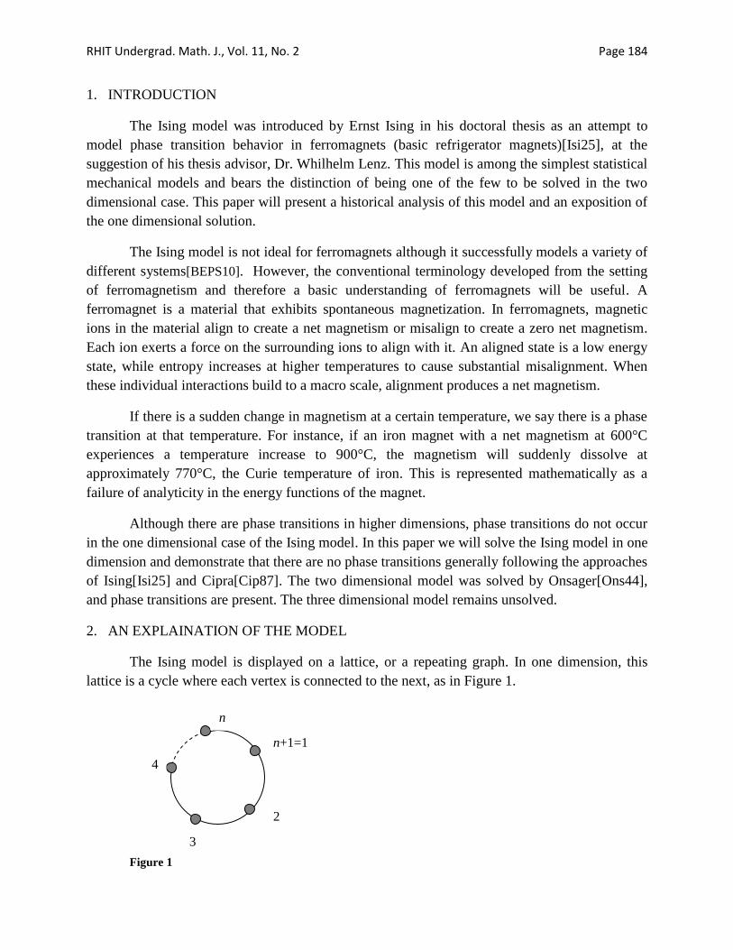
2. AN EXPLAINATION OF THE MODEL

The Ising model is displayed on a lattice, or a repeating graph. In one dimension, this

lattice is a cycle where each vertex is connected to the next, as in Figure 1.

Figure 1

n+1=1

2

n

4

3

Page 185 RHIT Undergrad. Math. J., Vol. 11, No. 2

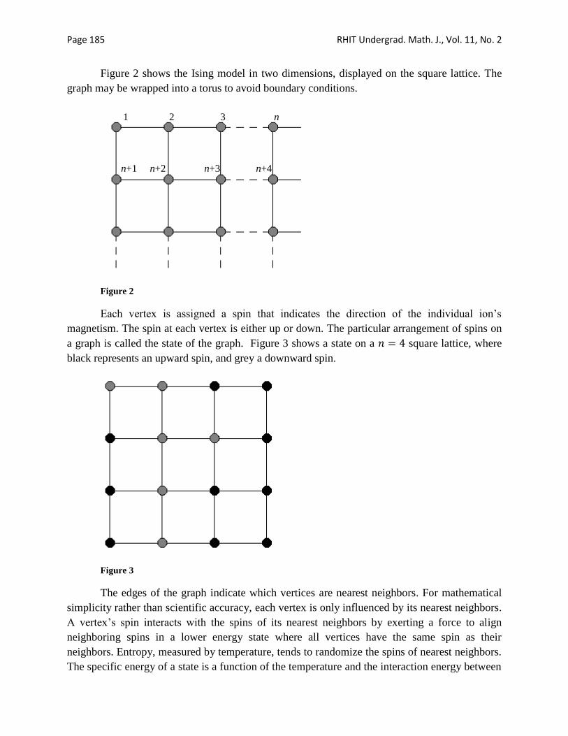
Figure 2 shows the Ising model in two dimensions, displayed on the square lattice. The

graph may be wrapped into a torus to avoid boundary conditions.

Figure 2

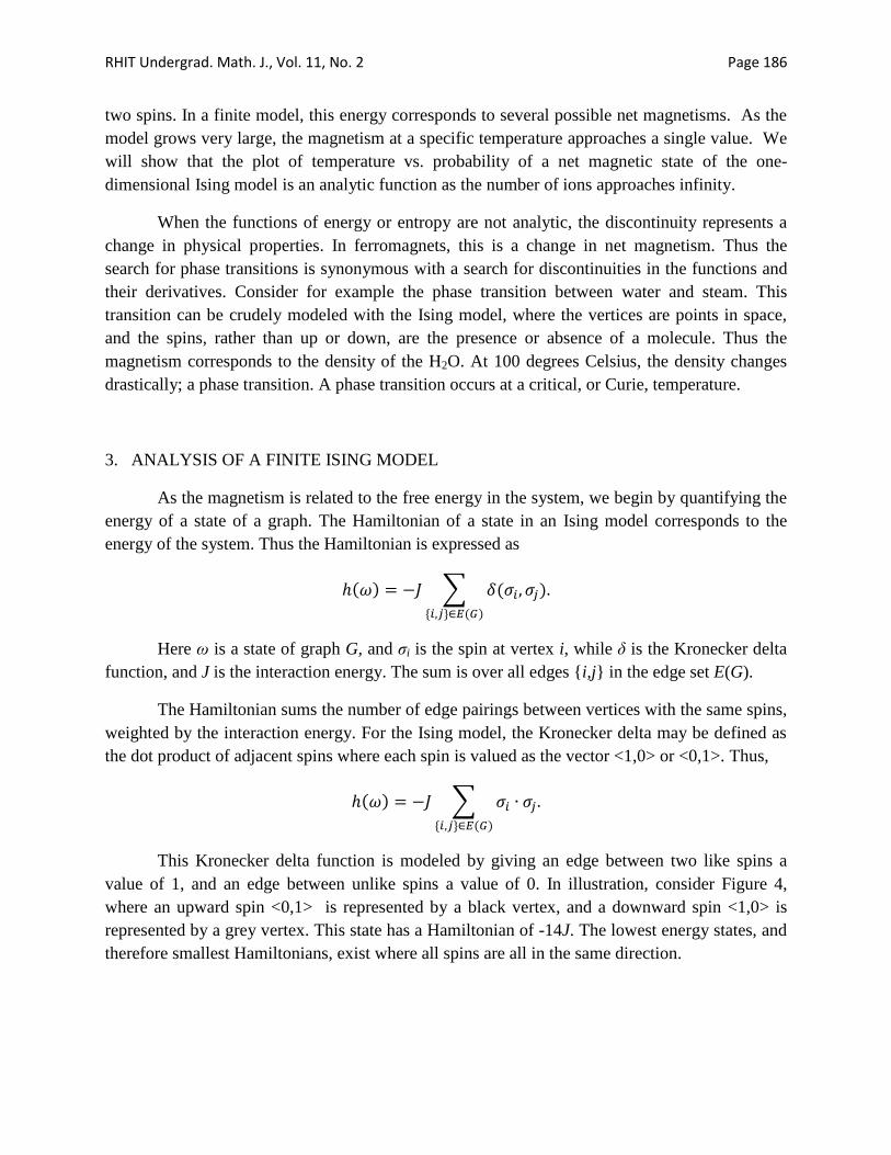
Each vertex is assigned a spin that indicates the direction of the individual ion’s

magnetism. The spin at each vertex is either up or down. The particular arrangement of spins on

a graph is called the state of the graph. Figure 3 shows a state on a square lattice, where

black represents an upward spin, and grey a downward spin.

Figure 3

The edges of the graph indicate which vertices are nearest neighbors. For mathematical

simplicity rather than scientific accuracy, each vertex is only influenced by its nearest neighbors.

A vertex’s spin interacts with the spins of its nearest neighbors by exerting a force to align

neighboring spins in a lower energy state where all vertices have the same spin as their

neighbors. Entropy, measured by temperature, tends to randomize the spins of nearest neighbors.

The specific energy of a state is a function of the temperature and the interaction energy between

1 2 3 n

n+1 n+2 n+3 n+4

RHIT Undergrad. Math. J., Vol. 11, No. 2 Page 186

two spins. In a finite model, this energy corresponds to several possible net magnetisms. As the

model grows very large, the magnetism at a specific temperature approaches a single value. We

will show that the plot of temperature vs. probability of a net magnetic state of the one-

dimensional Ising model is an analytic function as the number of ions approaches infinity.

When the functions of energy or entropy are not analytic, the discontinuity represents a

change in physical properties. In ferromagnets, this is a change in net magnetism. Thus the

search for phase transitions is synonymous with a search for discontinuities in the functions and

their derivatives. Consider for example the phase transition between water and steam. This

transition can be crudely modeled with the Ising model, where the vertices are points in space,

and the spins, rather than up or down, are the presence or absence of a molecule. Thus the

magnetism corresponds to the density of the H2O. At 100 degrees Celsius, the density changes

drastically; a phase transition. A phase transition occurs at a critical, or Curie, temperature.

3. ANALYSIS OF A FINITE ISING MODEL

As the magnetism is related to the free energy in the system, we begin by quantifying the

energy of a state of a graph. The Hamiltonian of a state in an Ising model corresponds to the

energy of the system. Thus the Hamiltonian is expressed as

( ) ∑ ( )

* + ( )

Here ω is a state of graph G, and σi is the spin at vertex i, while δ is the Kronecker delta

function, and J is the interaction energy. The sum is over all edges {i,j} in the edge set E(G).

The Hamiltonian sums the number of edge pairings between vertices with the same spins,

weighted by the interaction energy. For the Ising model, the Kronecker delta may be defined as

the dot product of adjacent spins where each spin is valued as the vector <1,0> or <0,1>. Thus,

( ) ∑

* + ( )

This Kronecker delta function is modeled by giving an edge between two like spins a

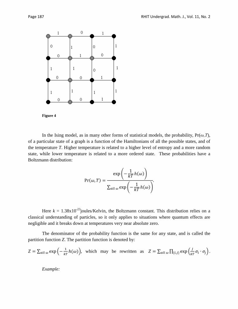
value of 1, and an edge between unlike spins a value of 0. In illustration, consider Figure 4,

where an upward spin <0,1> is represented by a black vertex, and a downward spin <1,0> is

represented by a grey vertex. This state has a Hamiltonian of -14J. The lowest energy states, and

therefore smallest Hamiltonians, exist where all spins are all in the same direction.

Page 187 RHIT Undergrad. Math. J., Vol. 11, No. 2

Figure 4

In the Ising model, as in many other forms of statistical models, the probability, Pr(ω,T),

of a particular state of a graph is a function of the Hamiltonians of all the possible states, and of

the temperature T. Higher temperature is related to a higher level of entropy and a more random

state, while lower temperature is related to a more ordered state. These probabilities have a

Boltzmann distribution:

( )

( ( ))

∑ ( ( ))

Here k = 1.38x10-23

joules/Kelvin, the Boltzmann constant. This distribution relies on a

classical understanding of particles, so it only applies to situations where quantum effects are

negligible and it breaks down at temperatures very near absolute zero.

The denominator of the probability function is the same for any state, and is called the

partition function Z. The partition function is denoted by:

∑ .

( )/ , which may be rewritten as ∑ ∏ .

/* +

Example:

RHIT Undergrad. Math. J., Vol. 11, No. 2 Page 188

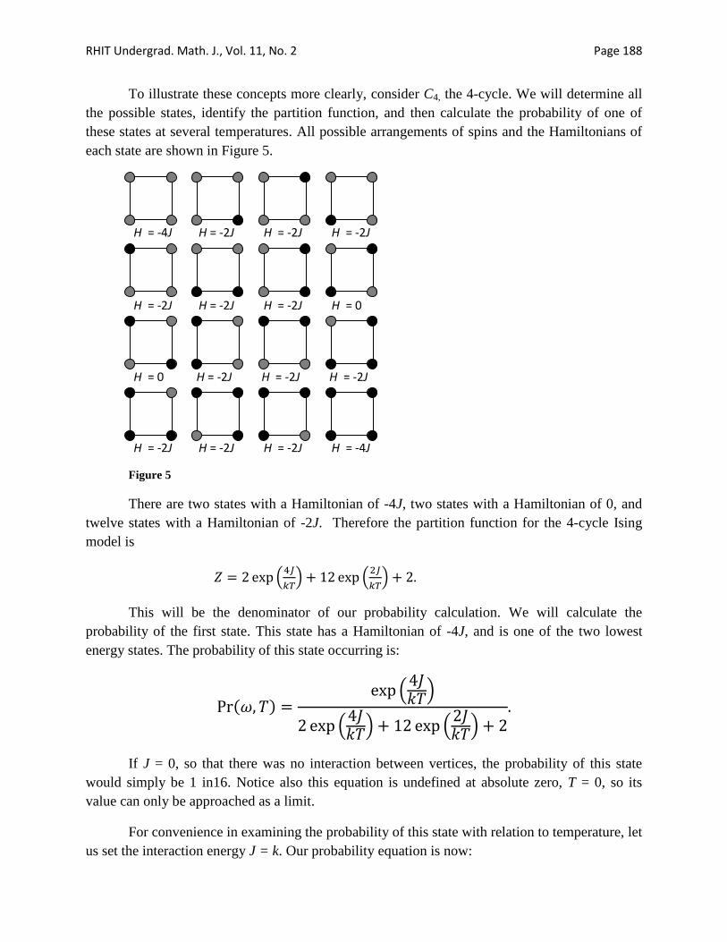
To illustrate these concepts more clearly, consider C4, the 4-cycle. We will determine all

the possible states, identify the partition function, and then calculate the probability of one of

these states at several temperatures. All possible arrangements of spins and the Hamiltonians of

each state are shown in Figure 5.

Figure 5

There are two states with a Hamiltonian of -4J, two states with a Hamiltonian of 0, and

twelve states with a Hamiltonian of -2J. Therefore the partition function for the 4-cycle Ising

model is

.

/ .

/

This will be the denominator of our probability calculation. We will calculate the

probability of the first state. This state has a Hamiltonian of -4J, and is one of the two lowest

energy states. The probability of this state occurring is:

( ) .

/

. / .

/

If J = 0, so that there was no interaction between vertices, the probability of this state

would simply be 1 in16. Notice also this equation is undefined at absolute zero, T = 0, so its

value can only be approached as a limit.

For convenience in examining the probability of this state with relation to temperature, let

us set the interaction energy J = k. Our probability equation is now:

H = -4J H = -2J H = -2J H = -2J

H = -2J H = -2J H = -2J H = 0

H = 0 H = -2J H = -2J H = -2J

H = -2J H = -2J H = -2J H = -4J

Page 189 RHIT Undergrad. Math. J., Vol. 11, No. 2

( ) (

)

. / .

/

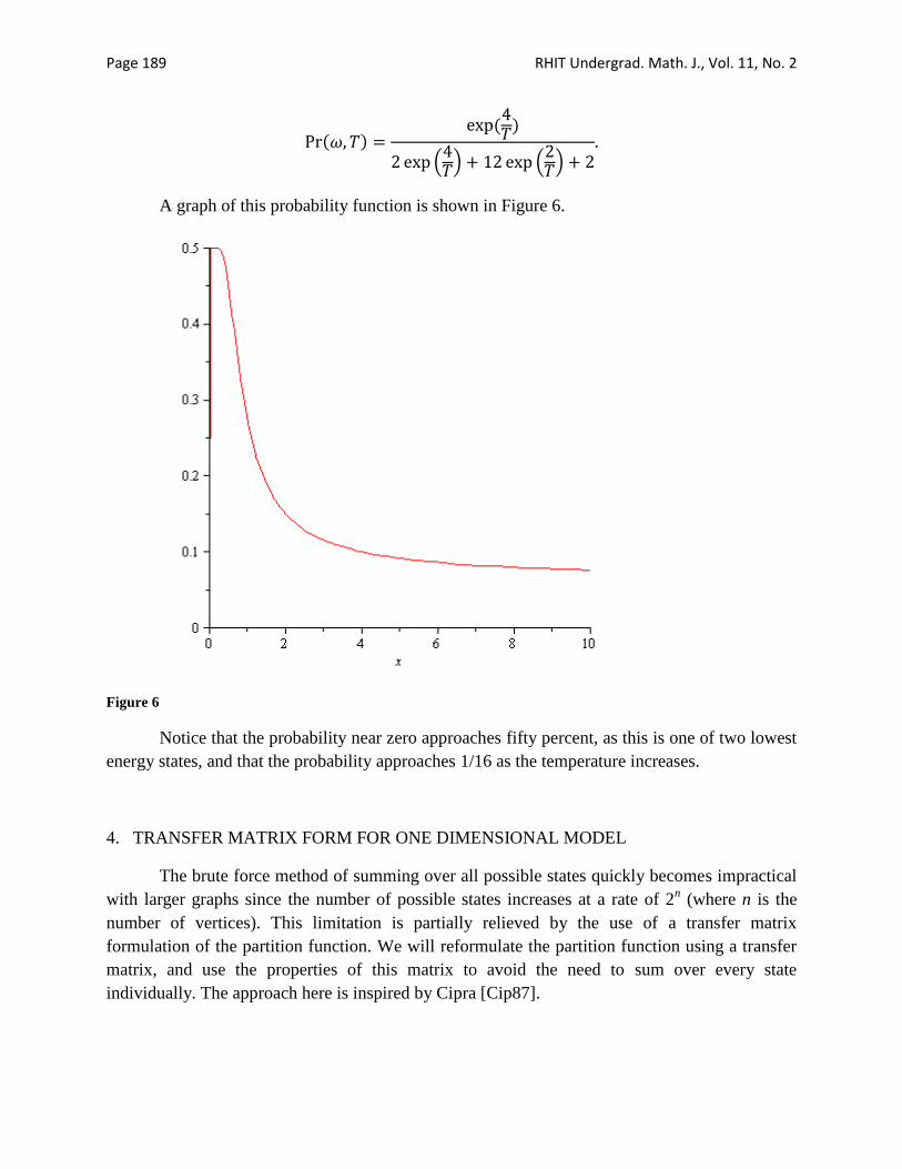
A graph of this probability function is shown in Figure 6.

Figure 6

Notice that the probability near zero approaches fifty percent, as this is one of two lowest

energy states, and that the probability approaches 1/16 as the temperature increases.

4. TRANSFER MATRIX FORM FOR ONE DIMENSIONAL MODEL

The brute force method of summing over all possible states quickly becomes impractical

with larger graphs since the number of possible states increases at a rate of 2n (where n is the

number of vertices). This limitation is partially relieved by the use of a transfer matrix

formulation of the partition function. We will reformulate the partition function using a transfer

matrix, and use the properties of this matrix to avoid the need to sum over every state

individually. The approach here is inspired by Cipra [Cip87].

RHIT Undergrad. Math. J., Vol. 11, No. 2 Page 190

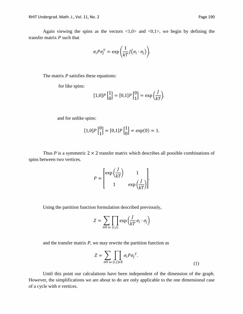
Again viewing the spins as the vectors <1,0> and <0,1>, we begin by defining the

transfer matrix P such that

(

( ))

The matrix P satisfies these equations:

for like spins:

, - 0 1 , - 0

1 (

*

and for unlike spins:

, - 0 1 , - 0

1 ( )

Thus P is a symmetric transfer matrix which describes all possible combinations of

spins between two vertices.

[ (

*

(

*

]

Using the partition function formulation described previously,

∑∏ (

*

* +

and the transfer matrix P, we may rewrite the partition function as

∑ ∏

* +

(1)

Until this point our calculations have been independent of the dimension of the graph.

However, the simplifications we are about to do are only applicable to the one dimensional case

of a cycle with n vertices.

Page 191 RHIT Undergrad. Math. J., Vol. 11, No. 2

With our graph a cycle of size n, we can expand Equation (1) and write:

∑ ∏

* +

∑

In order to format the equation for future simplification, factor the initial spin outside the

summation, creating two summands; one for when the initial spin is up and one when the spin is

down.

, - ( ∑

, -

) 0 1

, - ( ∑

, -

) 0 1

(2)

Since for any state where the initial spin is up, there is an otherwise identical state where

the spin is down, the two inner summations in this equation are equivalent.

This summation, ∑

, - is equal to P

n-1 by the

following induction argument:

If n = 2,

∑∏

0 1 , - 0

1 , -

If we assume that ∑ ∏

is true for some , then this argument also

holds for n+1 as follows.

First note that

∑∏

∑ (∏

+

Once again we split the equation into two summands, one for an upward spin on the

th vertex and one for a downward spin on the vertex.

∑∏

(∑ (∏

+

+ 0 1 , - (∑ (∏

+

+ 0 1 , -

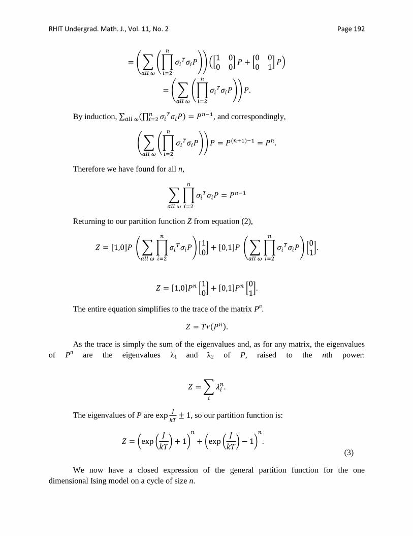
RHIT Undergrad. Math. J., Vol. 11, No. 2 Page 192

(∑ (∏

+

+ .0

1 0

1 /

(∑ (∏

+

+

By induction, ∑ (∏

) , and correspondingly,

(∑ (∏

+

+ ( )

Therefore we have found for all n,

∑∏

Returning to our partition function Z from equation (2),

, - (∑ ∏

+ 0 1 , - (∑ ∏

+ 0 1

, - 0 1 , - 0

1

The entire equation simplifies to the trace of the matrix Pn.

( )

As the trace is simply the sum of the eigenvalues and, as for any matrix, the eigenvalues

of Pn are the eigenvalues λ1 and λ2 of P, raised to the nth power:

∑

The eigenvalues of P are

, so our partition function is:

( (

* *

( (

* *

(3)

We now have a closed expression of the general partition function for the one

dimensional Ising model on a cycle of size n.

Page 193 RHIT Undergrad. Math. J., Vol. 11, No. 2

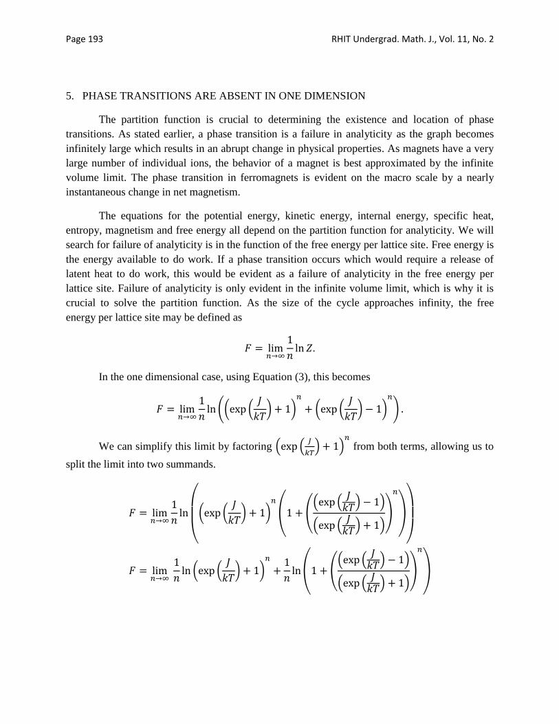
5. PHASE TRANSITIONS ARE ABSENT IN ONE DIMENSION

The partition function is crucial to determining the existence and location of phase

transitions. As stated earlier, a phase transition is a failure in analyticity as the graph becomes

infinitely large which results in an abrupt change in physical properties. As magnets have a very

large number of individual ions, the behavior of a magnet is best approximated by the infinite

volume limit. The phase transition in ferromagnets is evident on the macro scale by a nearly

instantaneous change in net magnetism.

The equations for the potential energy, kinetic energy, internal energy, specific heat,

entropy, magnetism and free energy all depend on the partition function for analyticity. We will

search for failure of analyticity is in the function of the free energy per lattice site. Free energy is

the energy available to do work. If a phase transition occurs which would require a release of

latent heat to do work, this would be evident as a failure of analyticity in the free energy per

lattice site. Failure of analyticity is only evident in the infinite volume limit, which is why it is

crucial to solve the partition function. As the size of the cycle approaches infinity, the free

energy per lattice site may be defined as

In the one dimensional case, using Equation (3), this becomes

(( (

* *

( (

* *

)

We can simplify this limit by factoring . .

/ /

from both terms, allowing us to

split the limit into two summands.

(

( (

* *

( (. .

/ /

. . / /

)

,

)

( (

* *

( (

. . / /

. . / /

)

,

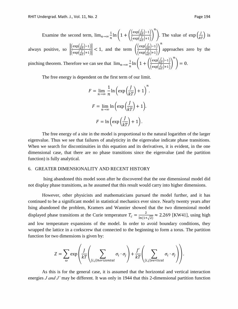
RHIT Undergrad. Math. J., Vol. 11, No. 2 Page 194

Examine the second term,

( (

. .

/ /

. .

/ /

)

). The value of .

/ is

always positive, so |. .

/ /

. .

/ /

| , and the term (. .

/ /

. .

/ /

)

approaches zero by the

pinching theorem. Therefore we can see that

( (

. .

/ /

. .

/ /

)

) .

The free energy is dependent on the first term of our limit.

( (

* *

( (

* *

( (

* *

The free energy of a site in the model is proportional to the natural logarithm of the larger

eigenvalue. Thus we see that failures of analyticity in the eigenvalue indicate phase transitions.

When we search for discontinuities in this equation and its derivatives, it is evident, in the one

dimensional case, that there are no phase transitions since the eigenvalue (and the partition

function) is fully analytical.

6. GREATER DIMENSIONALITY AND RECENT HISTORY

Ising abandoned this model soon after he discovered that the one dimensional model did

not display phase transitions, as he assumed that this result would carry into higher dimensions.

However, other physicists and mathematicians pursued the model further, and it has

continued to be a significant model in statistical mechanics ever since. Nearly twenty years after

Ising abandoned the problem, Kramers and Wannier showed that the two dimensional model

displayed phase transitions at the Curie temperature

( √ ) [KW41], using high

and low temperature expansions of the model. In order to avoid boundary conditions, they

wrapped the lattice in a corkscrew that connected to the beginning to form a torus. The partition

function for two dimensions is given by:

∑ (

( ∑ * +

)

( ∑ * +

),

As this is for the general case, it is assumed that the horizontal and vertical interaction

energies J and J’ may be different. It was only in 1944 that this 2-dimensional partition function

Page 195 RHIT Undergrad. Math. J., Vol. 11, No. 2

was actually solved by Onsager[Ons44]. In order to avoid boundary conditions, Onsager chose to

use the form of a straight torus instead of the corkscrew of Kramers and Wannier. The greatest

challenge in explaining and following the analysis of the two dimensional model is the sheer

number of summations and repeated operations required. In his original paper, Onsager defines

four operations on spins simply to keep his equations down to a reasonable size. In the two

dimensional case, the transfer matrix is infinite, representing the possibilities of a one

dimensional cross section of the two dimensional model. The ingenuity of Onsager’s approach is

in that he does not attempt to find a partition function that applies for any size 2-dimensional

model and then find its limit. Rather he begins directly with the infinite form. This allows him to

focus on only one eigenvector, as the other eigenvalues fall to zero in the infinite case[Ons44].

Solving greater dimensional cases, as well as the two dimensional case with an external

field, has proven extremely difficult. Noting the mathematical acrobatics Onsager managed in

order to solve the two dimensional model, it is tempting to believe that with sufficient creativity

and careful organizational choice the larger dimensional models can be solved. However, these

larger dimension problems are NP-complete. In 1982 Barahona[Bar82] showed that the three

dimensional and two dimensional with external field models are both NP-hard, as they are

equivalent to finding the maximum cardinality of a stable set in a planar cubic graph, a problem

known to be NP-hard[Bar82].

Istrail[Ist00] recently expanded Barahona’s conclusion. He identified an underlying graph

of the model, a Kuratowskian, in all non-planar varieties of the Ising model, and showed that due

to the nature of this graph all non-planar varieties of the Ising model are NP-complete, regardless

of whether the model itself was two or three dimensional. This conclusion applies to both the 3D

Ising model and non-planar 2D models, such as the 2D model with an external field or with next-

nearest neighbor interactions[Ist00]. Yet we cannot forget that it has not yet been proven that

NP-complete problems are unsolvable, so the Ising model may yet be solved for larger

dimensions, but an exact solution may be computationally intractable.

Nevertheless, significant work is done in specific cases of the problem, a variety of

generalizations of the model, and statistical and quantum analyses of unsolved versions. The

survey of [BEPS10] provides an overview of more recent applications and generalizations of the

Ising model.

REFERENCES

[Bar82] F. Barahona. (1982) J. Phys. A: Math. Gen. 15 3241.

[BEPS10] L. Beaudin, J. Ellis-Monaghan, G. Pangborn, R. Shrock (2010) “A Little

Statistical Mechanics for the Graph Theorist.” Discrete Mathematics, Vol.

310, Issues 13-14, pp. 2037-2053.

RHIT Undergrad. Math. J., Vol. 11, No. 2 Page 196

[Cip87] B. A. Cipra.(1987) “An Introduction to the Ising Model.” The American

Mathematical Monthly, Vol. 94, No. 10 (Dec.) pp. 937-959, MAA.

[Isi25] E. Ising, (1925), “Beitrag zur Theorie des Ferromagnetismus”, Z. Phys.

31: 253–258.

[Ist00] S. Istrail, (2000) “Statistical mechanics, three-dimensionality and NP-

completeness: I. Universality of intracatability for the partition function of

the Ising model across non-planar surfaces (extended abstract)”,

Proceedings of the thirty-second annual ACM symposium on Theory of

computing, p.87-96, May 21-23, Portland, Oregon.

[KW41] H. A. Kramers and G. H. Wannier (1941). “Statistics of the two-

dimensional ferromagnet”. Physical Review 60: 252–262.

[Ons44] L. Onsager, (1944), “Crystal statistics. I. A two-dimensional model with

an order-disorder transition”, Physical Review (2) 65: 117–149.