PhD Showcase: Automated artifact-free seafloor surfacereconstruction with two-step ODETLAP

PhD Student: Tsz-Yam LauRensselaer Polytechnic Institute

110, Eighth StreetTroy, NY, USA

laut@cs.rpi.edu

PhD supervisor: W. Randolph FranklinRensselaer Polytechnic Institute

110, Eighth StreetTroy, NY, USA

mail@wrfranklin.org

ABSTRACTWe present an updated artifact-free seafloor surface recon-struction scheme which preserves more terrain features thanour previous attempt using overdetermined Laplacian Par-tial Differential Equation (ODETLAP) and automates theadjustment of smoothing parameter. The high resolutionversion of such a surface fitting problem remains a challengesince we are still confined to extremely unevenly distributeddepth samples collected along and near the ships, in whichcase numerous generic reconstruction algorithms generateunacceptable surfaces featuring abnormal depth fluctuationswhich are correlated with the trackline locations. Previouslywe reported the use a modified ODETLAP scheme, whichintegrates data-density-dependent smoothing into the recon-struction process, to generate surfaces which are free fromsuch acquisition footprint. However, that scheme still suffersfrom terrain feature loss due to smoothing, and the relianceof human to decide appropriate smoothing factor. This paperaims to fix these two problems with a two-step ODETLAPprocedure. The procedure first applies an accuracy-biasedODETLAP to complete the missing depth data from thegiven samples. After that, the vigorous depth fluctuationsalong the tracklines are removed by applying a smoothing-biased ODETLAP on the completed depth grid. To decidethe optimal smoothing factor automatically, the procedurecomputes the areas of the individual bumps on the recon-structed surface. A surface suffering heavily from the artifactshas many small bumps but few big ones. Smoothing reducessuch skewness. We find that for many datasets, the artifactis mostly gone when the coefficient of variation of the areasdrops to around 1.3. Using that value to gauge the smoothingfactor, the automated scheme successfully generates artifact-free seafloor surfaces within a limited error budget.

Categories and Subject DescriptorsI.3.5 [Computing Methodologies]: Computer GraphicsComputational Geometry and Object Modeling

The SIGSPATIAL Special, Volume 4, Number 3, November 2012.Copyright is held by the author/owner(s).

KeywordsGIS, ODETLAP, bathymetry, surface reconstruction, sparseheight grid

1. INTRODUCTIONA bathymetric chart, the underwater equivalent of a to-pographic map, represents the depth and features of theocean floor. This data helps solve not only applications suchas tsunami hazard assessment, communications cable andpipeline route planning, resource exploration, habitat man-agement, and territorial claims under the Law of the Sea,but also fundamental Earth science questions, such as whatcontrols seafloor shape and how seafloor shape influencesglobal climate [12].

While wide-area, high-resolution ground heights can now bemeasured quickly with aerial electromagnetic survey tech-nologies such as standard photogrammetry and LIDAR [10],the same is not true with seafloor depths. Good discussionson this issue are available at [12, 13]. In short, the problemlies in the 3000-5000 meters of salty water which masks thepenetration of electromagnetic waves.

The altimeter method is an attempt for wide-area coverage.The method exploits the fact that the ocean surface hasbroad bumps and dips that mimic the topography of theocean floor. By surveying the shape of the water surfaceinstead, we avoid the need of shooting electromagnetic wavesinto the water, yet allowing us to deduce how the underlyingseafloor looks like. However, features on the ocean floor thatare narrower than the average ocean depth of 3-5 kilometersdo not produce measurable bumps on the ocean surface.

To obtain high-resolution data, we have no choice but to sailacross the ocean, and on the way send out acoustic pulsesto the seafloor. From the time it takes the pulses to leavethe ship, be reflected by the seafloor and eventually get backthe ship again, the ocean depths can be estimated. However,since ships travel slowly, the ocean remains largely uncharted.It has been estimated that 300 years are needed to coverthe whole ocean area. With the most popular multibeambathymetry technique [15], we can collect many data pointswith 10m resolution in a swath up to 10km wide along a ship’strackline. However, between the tracklines there is no data.In the southern oceans, these survey lines can sometimes beclose together, but more often they are hundreds of kilometersapart [14]. Figure 1 demonstrates the spatial distribution ofsuch shipboard data samples in a few 10 × 10 degree regions.

Figure 1: Locations with available depth samples.(Top left) Region 1: 30S-40S, 90E-100E. (Top right)Region 2: 40S-50S, 80E-90E. (Bottom) Region 3:40S-50S, 90E-100E.

Since a full data grid is assumed for many terrain analyses,we need a surface reconstruction. The problem is definedover a spatial domain of dimensions n× n. Available are themeasured depth values of k � n2 positions (x1, y1), (x2, y2),. . . , (xk, yk), denoted as hx1,y1 , hx2,y2 , . . . , hxk,yk . The taskis to predict the depths for all the n × n positions in thedomain, including those of the k known positions and thoseof the remaining n2 − k unknown positions. This assumesfor each possible location (i, j), the corresponding predicteddepth zi,j is single-valued; caves or overhangs are not allowed.

Acquisition footprint is the major problem of using generalreconstruction schemes on those extremely unevenly dis-tributed depth data, even with a few current bathymetrycharts such as the one published by National Oceanic andAtmospheric Administration (NOAA) [9]. It refers to theartifact which makes the tracklines visible. The artifact isespecially obvious under shaded relief, a graphic techniquewhich is often used to highlight terrain surface variations [17].Figure 2 shows how the reconstructed seafloor surfaces looklike under a few such schemes such as Kriging [4] and naturalneighbor [16]. While both come up with a surface of a similargeneral shape, we observe abnormal high-frequency depthfluctuations which are correlated with the few trackline loca-tions. We aim at a surface from which we cannot deduce thetrackline locations. Meanwhile, its general shape as portrayedby relatively low frequencies should be preserved.

To remove the artifact, a typical routine is to smooth thereconstructed surface. The difficulty lies in the fact that itis not a simple high-frequency removal problem. Each localregion has its unique smoothing requirement. We may notneed to smooth certain noisy trackline locations, as long astheir neighborhood is equally noisy. In contrast, we cannotaccept even small fluctuations along the tracklines if they

are surrounded by relatively calm surfaces which make thetracklines stand out. One known attempt, CleanTOPO2 [11],involves post-processing, manually removing the artifactswith repeated applications of a morphological averaging fil-ter. Though easy for humans to decide where filtering shouldbe done and when to stop, the process is subjective andtime-consuming. As we are obtaining new trackline depthdata from time to time, it may become impractical to do sucha manual process every time the database expands. This mo-tivates the automation of artifact-free surface reconstruction.

Figure 2: Region 1 reconstructions with (Left) Krig-ing, (Right) natural neighbor.

Our previous work proposed Overdetermined Laplacian Par-tial Differential Equation (ODETLAP) as a partial solution.Its original version was designed with smoothing consideredright in the reconstruction process, and yields much bet-ter reconstruction accuracy than conventional algorithm. Atthat time, we further improved its accuracy by allowing thesmoothing factor to vary according to local smoothing need.Section 2 will give information about this solution.

This paper aims to improve that ODETLAP implementationin two ways. First, we find that quite a few terrain featureshave been lost in the above variable-smoothing ODETLAP.We fix it by a two-step approach which reconstructs a pre-liminary surface with ODETLAP of a high-accuracy setting,and then applying a smoothing-biased ODETLAP over thatpreliminary surface. Second, our previously-reported imple-mentation relied on human to set smoothing parameters. Weautomate the process based on the bump area distribution.Details will be given in Section 3, before we conclude thepaper in Section 4.

2. ODETLAPWe first presented Overdetermined Laplacian Partial Differ-ential Equation (ODETLAP) as a superior above-groundterrain reconstruction and lossy terrain compression [2, 20,21], since it predicts neighboring terrain heights better thanother conventional prediction schemes. Besides, it can workwith contour lines (continuous or intermittently broken), infermountain tops inside a ring of contours, and enforce continu-ity of slope across contours. All these are favorable featuresof natural-looking terrains.

Its formulation sets up an overdetermined system Az = b, asshown in Figure 3, to solve for the depths of the whole seafloordepth grid z in the bathymetry case presented here. Thesystem includes an exact equation for each of the k known-depth positions. That equation aims to set the depth value

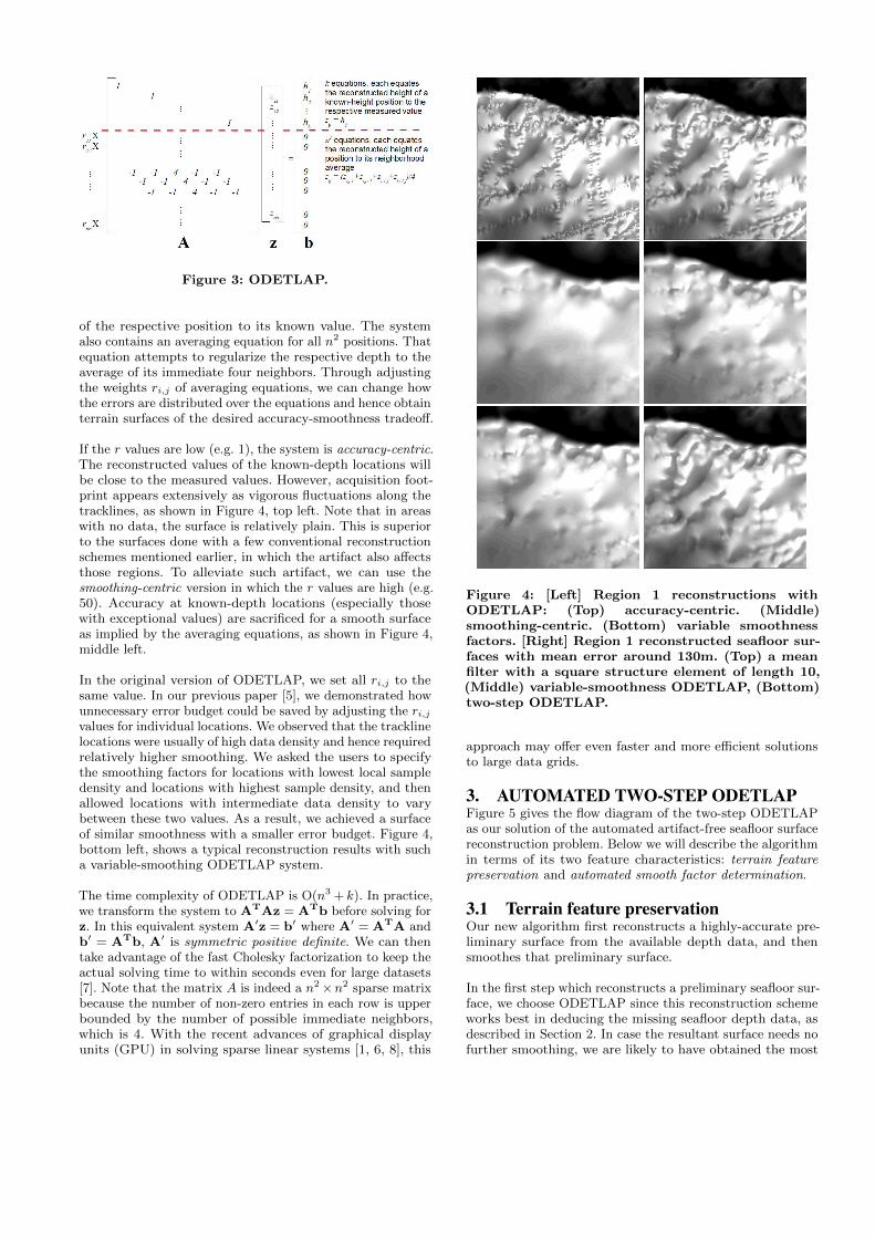
Figure 3: ODETLAP.

of the respective position to its known value. The systemalso contains an averaging equation for all n2 positions. Thatequation attempts to regularize the respective depth to theaverage of its immediate four neighbors. Through adjustingthe weights ri,j of averaging equations, we can change howthe errors are distributed over the equations and hence obtainterrain surfaces of the desired accuracy-smoothness tradeoff.

If the r values are low (e.g. 1), the system is accuracy-centric.The reconstructed values of the known-depth locations willbe close to the measured values. However, acquisition foot-print appears extensively as vigorous fluctuations along thetracklines, as shown in Figure 4, top left. Note that in areaswith no data, the surface is relatively plain. This is superiorto the surfaces done with a few conventional reconstructionschemes mentioned earlier, in which the artifact also affectsthose regions. To alleviate such artifact, we can use thesmoothing-centric version in which the r values are high (e.g.50). Accuracy at known-depth locations (especially thosewith exceptional values) are sacrificed for a smooth surfaceas implied by the averaging equations, as shown in Figure 4,middle left.

In the original version of ODETLAP, we set all ri,j to thesame value. In our previous paper [5], we demonstrated howunnecessary error budget could be saved by adjusting the ri,jvalues for individual locations. We observed that the tracklinelocations were usually of high data density and hence requiredrelatively higher smoothing. We asked the users to specifythe smoothing factors for locations with lowest local sampledensity and locations with highest sample density, and thenallowed locations with intermediate data density to varybetween these two values. As a result, we achieved a surfaceof similar smoothness with a smaller error budget. Figure 4,bottom left, shows a typical reconstruction results with sucha variable-smoothing ODETLAP system.

The time complexity of ODETLAP is O(n3 + k). In practice,we transform the system to ATAz = ATb before solving forz. In this equivalent system A′z = b′ where A′ = ATA andb′ = ATb, A′ is symmetric positive definite. We can thentake advantage of the fast Cholesky factorization to keep theactual solving time to within seconds even for large datasets[7]. Note that the matrix A is indeed a n2 ×n2 sparse matrixbecause the number of non-zero entries in each row is upperbounded by the number of possible immediate neighbors,which is 4. With the recent advances of graphical displayunits (GPU) in solving sparse linear systems [1, 6, 8], this

Figure 4: [Left] Region 1 reconstructions withODETLAP: (Top) accuracy-centric. (Middle)smoothing-centric. (Bottom) variable smoothnessfactors. [Right] Region 1 reconstructed seafloor sur-faces with mean error around 130m. (Top) a meanfilter with a square structure element of length 10,(Middle) variable-smoothness ODETLAP, (Bottom)two-step ODETLAP.

approach may offer even faster and more efficient solutionsto large data grids.

3. AUTOMATED TWO-STEP ODETLAPFigure 5 gives the flow diagram of the two-step ODETLAPas our solution of the automated artifact-free seafloor surfacereconstruction problem. Below we will describe the algorithmin terms of its two feature characteristics: terrain featurepreservation and automated smooth factor determination.

3.1 Terrain feature preservationOur new algorithm first reconstructs a highly-accurate pre-liminary surface from the available depth data, and thensmoothes that preliminary surface.

In the first step which reconstructs a preliminary seafloor sur-face, we choose ODETLAP since this reconstruction schemeworks best in deducing the missing seafloor depth data, asdescribed in Section 2. In case the resultant surface needs nofurther smoothing, we are likely to have obtained the most

Figure 5: Two-step ODETLAP workflow.

SRTM1 Natural neighbor ODETLAPW121N38

31m (413m) 24m (292m)1201:1600,1201:1600

W121N3820m (309m) 18m (242m)

2800:3200, 801:1200W121N38

17m (299m) 15m (164m)3201:3600, 401:800

W111N314m (93m) 3m (79m)

401:800, 1:400W111N31

14m (173m) 11m (120m)401:800, 401:800

W111N315m (134m) 4m (134m)

401:800, 801:1200

Table 1: Mean errors and maximum errors (in paren-theses) of the terrain surfaces reconstructed usingheight samples on the tracklines of Region 1.

accurate surface. We set the weighting between the exactequations and the averaging equations to 1:1. Beyond thatpoint, increasing the weightings of the exact equations doesnot change the accuracy of the preliminary terrain too much.

To investigate the effect of switching the terrain reconstruc-tion scheme in the first step from ODETLAP to the others,we first remove the height values of a few full terrains exceptthose falling on the tracklines shown in Figure 1. (Note wedo not use seafloor surfaces as no ground truth is availablefor error comparison.) Then we reconstruct the terrain withdifferent techniques and compute the errors with respect tothe ground truth. ODETLAP does the best in guessing themissing heights, as reflected by the generally lower meanerrors and maximum errors shown in Table 1. This resultsupports our choice of ODETLAP even if we are now workingon extremely unevenly distributed depth samples.

In the second step which smoothes the preliminary surface,we once again pick ODETLAP since this scheme providesbetter smoothing of the artifacts than others under the sameerror budget. Figure 4, right, compares the smoothing resultswith a mean filter (similar to the one used in CleanTOPO2mentioned in Section 2) and ODETLAP under similar errorbudget. While the acquisition artifact is almost gone withODETLAP smoothing, it is not the case with the mean filter.Table 2 shows the respective mean error budgets neededby the sample seafloors to achieve the respective optimalsmoothing levels (using the metric defined in the next sub-section). Our ODETLAP smoothing scheme just needs halfof the error budget as the average filter counterpart. Theresults above demonstrate the capability of our scheme in

Region ODETLAP Mean filterRegion 1 130m 297mRegion 2 75m 178mRegion 3 214m 360m

Table 2: Mean error budgets to reach optimalsmoothing levels.

distributing the limited error budget to smoothing locations.

The only variable of this algorithm is the smoothing factorin the second step. Figures 6–8, left, show how the surfacevaries as smoothing increases. A higher smoothing factormeans a higher mean error but at the same time bettersmoothing-out of the small bumps along the tracklines. Whencompared with our original implementation which requiresthe specification of the lower and upper smoothing factors, wenow have one fewer degree of freedom, make it easier to adjust.Also note that on raising the error budget, the high-frequencyacquisition footprint is gone before those lower-frequencyterrain features which account for the general terrain shape.Such a smoothing priority makes the scheme superior over ourpreviously-proposed variable-smoothing ODETLAP. In thesurface reconstructed with variable-smoothing ODETLAPsuch as the one in Figure 4 middle right, even though theacquisition footprint is also almost gone, we also lose quite afew terrain features.

3.2 Automated smoothing determinationThe above two-step procedure features a single parametercontrolling the smoothing of the final reconstructed seafloorsurface. To allow automated determination of the optimalsmoothing level, first we need to convert the acquisitionfootprint to a form that is recognizable by computers. Afterseveral experiments, we find that the graph of Gaussiancurvature may be used. As shown on the right hand side ofFigures 6–8, the artifact appears as relatively small patchesof positive Gaussian curvature concentrated at the tracklinelocations. In fact, patches of Gaussian curvature is regardedas a view-independent indicator of regions with potentialshaded relief in a few other research [3].

As observed from the same set of figures, smoothing helpsenlarge those patches or simply remove them. With a smallsmoothing factor, along the tracklines we have a huge numberof small such patches. This is in contrast with regions with nodata where there are few, much bigger patches. On increasingsmoothing, mean error at known-height location increases.Meanwhile, the bumps along the tracklines become fewerand bigger, while those in no-data regions hardly change interms of both size and quantity. This leads to a drop of thevariations among the patch areas.

To utilize the above phenomenon in automated smoothingfactor determination, we first apply a morphological erosion[19] with a 3-pixel-width square component on the positiveGaussian curvature graph to help discriminate the patches.We then compute the coefficient of variation cv, which is anormalized measure of dispersion of a probability distribution[18], of the patch areas. The acquisition footprint is foundto be almost gone when that coefficient drops to around 1.3.Figures 6–8, bottom, correspond to a smoothing level with

Figure 6: (Left) Region 1 reconstructed seafloor sur-faces. (Right) Respective positive Gaussian curva-ture locations. The mean errors, from top to bottom,are around 44m, 78m and 130m respectively.

around that coefficient value. Note that different datasetsmay need different error budgets to remove the artifacts. Forexample, while Region 3 requires a mean error budget ashigh as 214m to have the artifact removed, Region 2 needs75m only. Using that coefficient as a gauge helps reduceunnecessary smoothing and hence reduce the errors neededto achieve an artifact-free surface.

4. CONCLUSIONWe have presented an improved ODETLAP procedure forthe automated reconstruction of artifact-free seafloor sur-faces within a limited error budget. It has the smoothingfactor as its only parameter, making it easier to adjust thanour previous attempt which requires two parameter inputs.By smoothing an accurate reconstruction with ODETLAP,we allow terrain features to be better preserved than ourpreviously-reported scheme that reconstructs from the givenmeasured values directly. To automate the adjustment of thesmoothness parameter, we analyze the Gaussian curvatureof the reconstructed surfaces. Areas of positive Gaussiancurvatures highly resemble the locations of the bumps thatwe observe on the shaded reconstructed surface. Increasingsmoothing enlarges the small bumps and reduces their num-bers along the tracklines, thus alleviating the acquisition

Figure 7: (Left) Region 2 reconstructed seafloor sur-faces. (Right) Respective positive Gaussian curva-ture locations. The mean errors, from top to bottom,are around 43m, 55m and 75m respectively.

footprint. When the coefficient of variation of such areas isaround 1.3, the artifact is almost gone. We use this observa-tion to determine the minimum smoothing needed for theartifact-free surface.

In the future, we will look into the automatic stopping crite-rion further. More tests will be done on a variety of tracklinedepth samples. Even more accurate stopping criteria willbe investigated. Our current work embraces data from thetracklines but not the altimeter. It is interesting to see howdata from different sources could combine.

This research was partially supported by NSF grants CMMI-0835762 and IIS-1117277.

5. REFERENCES[1] N. Bell and M. Garland. Implementing sparse

matrix-vector multiplication on throughput-orientedprocessors. In Proceedings of the Conference on HighPerformance Computing Networking, Storage andAnalysis, SC ’09, pages 18:1–18:11, New York, NY,USA, 2009. ACM.

[2] M. B. Gousie and W. R. Franklin. Augmentinggrid-based contours to improve thin plate DEM

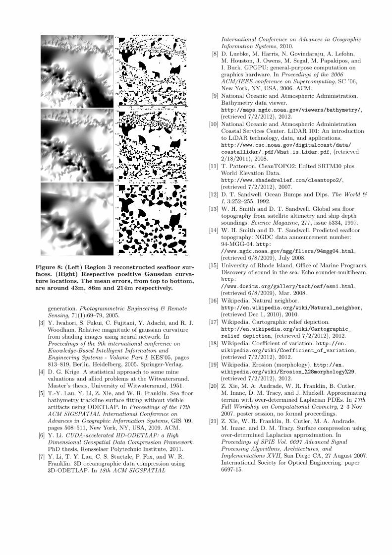
Figure 8: (Left) Region 3 reconstructed seafloor sur-faces. (Right) Respective positive Gaussian curva-ture locations. The mean errors, from top to bottom,are around 43m, 86m and 214m respectively.

generation. Photogrammetric Engineering & RemoteSensing, 71(1):69–79, 2005.

[3] Y. Iwahori, S. Fukui, C. Fujitani, Y. Adachi, and R. J.Woodham. Relative magnitude of gaussian curvaturefrom shading images using neural network. InProceedings of the 9th international conference onKnowledge-Based Intelligent Information andEngineering Systems - Volume Part I, KES’05, pages813–819, Berlin, Heidelberg, 2005. Springer-Verlag.

[4] D. G. Krige. A statistical approach to some minevaluations and allied problems at the Witwatersrand.Master’s thesis, University of Witwatersrand, 1951.

[5] T.-Y. Lau, Y. Li, Z. Xie, and W. R. Franklin. Sea floorbathymetry trackline surface fitting without visibleartifacts using ODETLAP. In Proceedings of the 17thACM SIGSPATIAL International Conference onAdvances in Geographic Information Systems, GIS ’09,pages 508–511, New York, NY, USA, 2009. ACM.

[6] Y. Li. CUDA-accelerated HD-ODETLAP: a HighDimensional Geospatial Data Compression Framework.PhD thesis, Rensselaer Polytechnic Institute, 2011.

[7] Y. Li, T. Y. Lau, C. S. Stuetzle, P. Fox, and W. R.Franklin. 3D oceanographic data compression using3D-ODETLAP. In 18th ACM SIGSPATIAL

International Conference on Advances in GeographicInformation Systems, 2010.

[8] D. Luebke, M. Harris, N. Govindaraju, A. Lefohn,M. Houston, J. Owens, M. Segal, M. Papakipos, andI. Buck. GPGPU: general-purpose computation ongraphics hardware. In Proceedings of the 2006ACM/IEEE conference on Supercomputing, SC ’06,New York, NY, USA, 2006. ACM.

[9] National Oceanic and Atmospheric Administration.Bathymetry data viewer.http://maps.ngdc.noaa.gov/viewers/bathymetry/,(retrieved 7/2/2012), 2012.

[10] National Oceanic and Atmospheric AdministrationCoastal Services Center. LiDAR 101: An introductionto LiDAR technology, data, and applications.http://www.csc.noaa.gov/digitalcoast/data/

coastallidar/_pdf/What_is_Lidar.pdf, (retrieved2/18/2011), 2008.

[11] T. Patterson. CleanTOPO2: Edited SRTM30 plusWorld Elevation Data.http://www.shadedrelief.com/cleantopo2/,(retrieved 7/2/2012), 2007.

[12] D. T. Sandwell. Ocean Bumps and Dips. The World &I, 3:252–255, 1992.

[13] W. H. Smith and D. T. Sandwell. Global sea floortopography from satellite altimetry and ship depthsoundings. Science Magazine, 277, issue 5334, 1997.

[14] W. H. Smith and D. T. Sandwell. Predicted seafloortopography: NGDC data announcement number:94-MGG-04. http://www.ngdc.noaa.gov/mgg/fliers/94mgg04.html,(retrieved 6/8/2009), July 2008.

[15] University of Rhode Island, Office of Marine Programs.Discovery of sound in the sea: Echo sounder-multibeam.http:

//www.dosits.org/gallery/tech/osf/esm1.html,(retrieved 6/8/2009), Mar. 2008.

[16] Wikipedia. Natural neighbor.http://en.wikipedia.org/wiki/Natural_neighbor,(retrieved Dec 1, 2010), 2010.

[17] Wikipedia. Cartographic relief depiction.http://en.wikipedia.org/wiki/Cartographic_

relief_depiction, (retrieved 7/2/2012), 2012.

[18] Wikipedia. Coefficient of variation. http://en.wikipedia.org/wiki/Coefficient_of_variation,(retrieved 7/2/2012), 2012.

[19] Wikipedia. Erosion (morphology). http://en.wikipedia.org/wiki/Erosion_%28morphology%29,(retrieved 7/2/2012), 2012.

[20] Z. Xie, M. A. Andrade, W. R. Franklin, B. Cutler,M. Inanc, D. M. Tracy, and J. Muckell. Approximatingterrain with over-determined Laplacian PDEs. In 17thFall Workshop on Computational Geometry, 2–3 Nov2007. poster session, no formal proceedings.

[21] Z. Xie, W. R. Franklin, B. Cutler, M. A. Andrade,M. Inanc, and D. M. Tracy. Surface compression usingover-determined Laplacian approximation. InProceedings of SPIE Vol. 6697 Advanced SignalProcessing Algorithms, Architectures, andImplementations XVII, San Diego CA, 27 August 2007.International Society for Optical Engineering. paper6697-15.