Embed Size (px)
Citation preview

Analytical Query Execution Optimized for all Layers of Modern Hardware
1
Orestis Polychroniou
PhD Thesis Defense
Ορέστης Πολυχρονίου

Big Data
❖ Volume and value of (big) data❖ 20 zettabytes of data by 2020
❖ $125 billion in 2015
❖ $40 billion for databases
❖ Relational Analytics❖ Business Intelligence
❖ Decision Support
❖ > $10 billion market
2

Database Systems
3
❖ Disk-based / Traditional DBMS❖ Data on (hard) disk
❖ Query execution disk-bound
❖ Not very distributed (e.g. Oracle)
❖ In-Memory / “Modern” DBMS❖ Data (mostly) in RAM
❖ Query execution memory-bound
❖ Very distributed (e.g. cloud)
new hardware !

Impact of Hardware❖ Traditional —> Modern DBMS
❖ Driven by hardware advances !
❖ Hardware advances affecting databases❖ Large main memory capacity
❖ Complex multi-core processors
❖ Scalable memory hierarchy (including fast networks)
❖ How can we achieve high performance in a modern database ?❖ Database system specialization
❖ Adapting to the hardware dynamics
4
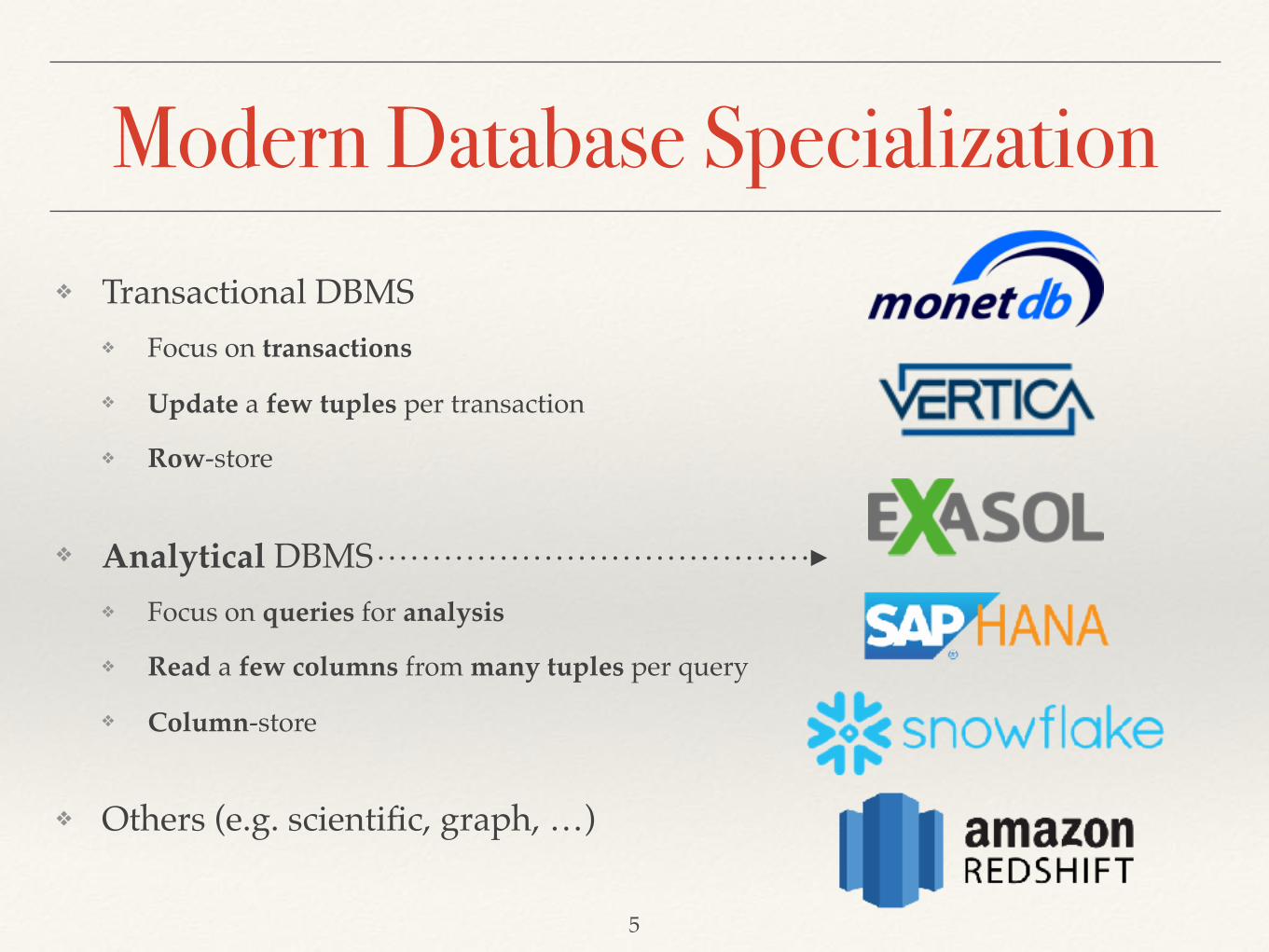
Modern Database Specialization❖ Transactional DBMS
❖ Focus on transactions
❖ Update a few tuples per transaction
❖ Row-store
❖ Analytical DBMS❖ Focus on queries for analysis
❖ Read a few columns from many tuples per query
❖ Column-store
❖ Others (e.g. scientific, graph, …)
5
Research Statement
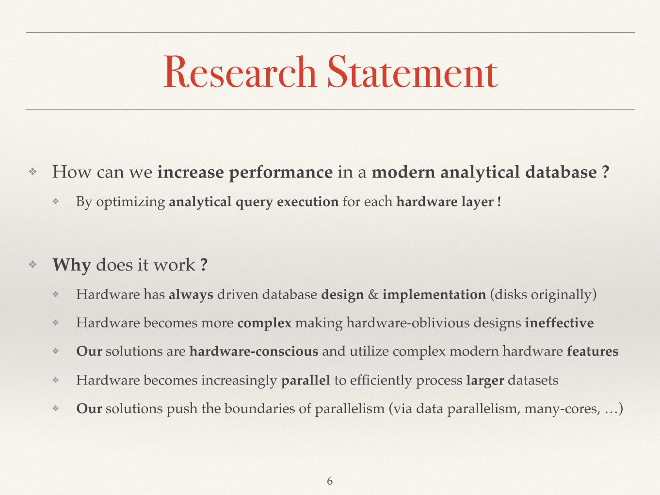
❖ How can we increase performance in a modern analytical database ?❖ By optimizing analytical query execution for each hardware layer !
❖ Why does it work ?❖ Hardware has always driven database design & implementation (disks originally)
❖ Hardware becomes more complex making hardware-oblivious designs ineffective
❖ Our solutions are hardware-conscious and utilize complex modern hardware features
❖ Hardware becomes increasingly parallel to efficiently process larger datasets
❖ Our solutions push the boundaries of parallelism (via data parallelism, many-cores, …)
6

Layers of Modern Hardware
7
CPU CPU
CPUCPU
RAM
RAM RAM
RAM
ServerServer Server
X
Server
Network
Core Core
CoreCore
core pipeline
CPU cache
main memory
NUMA
network

Modern Mainstream CPUs
❖ Thread parallelism❖ Multiple cores
❖ Multiple threads per core
❖ Instruction level parallelism❖ Out-of-order execution
❖ Super-scalar pipeline
❖ Data parallelism❖ SIMD vectorization
8
Core Core Core Core
Core Core Core Core
L3 cache
L1 cache
L2 cache
Pipeline

SIMD Vectorization
9
❖ As compiler optimization❖ Works for simple loops only
❖ Insufficient for database operators
for (i = 0; i < n; ++i) { c[i] = a[i] + b[i]; }
for (i = 0; i < n; i += 16) { __m512i x = _mm512_load_si512(&a[i]); __m512i y = _mm512_load_si512(&b[i]); __m512i z = _mm512_add_epi32(x, y); _mm512_store_si512(&c[i], z); }
scalar code
SIMD code
51 2 3 4 6 7 8
313 8 5 2 1 121
815 11 9 8 8 922
+
=
8-way SIMD addition
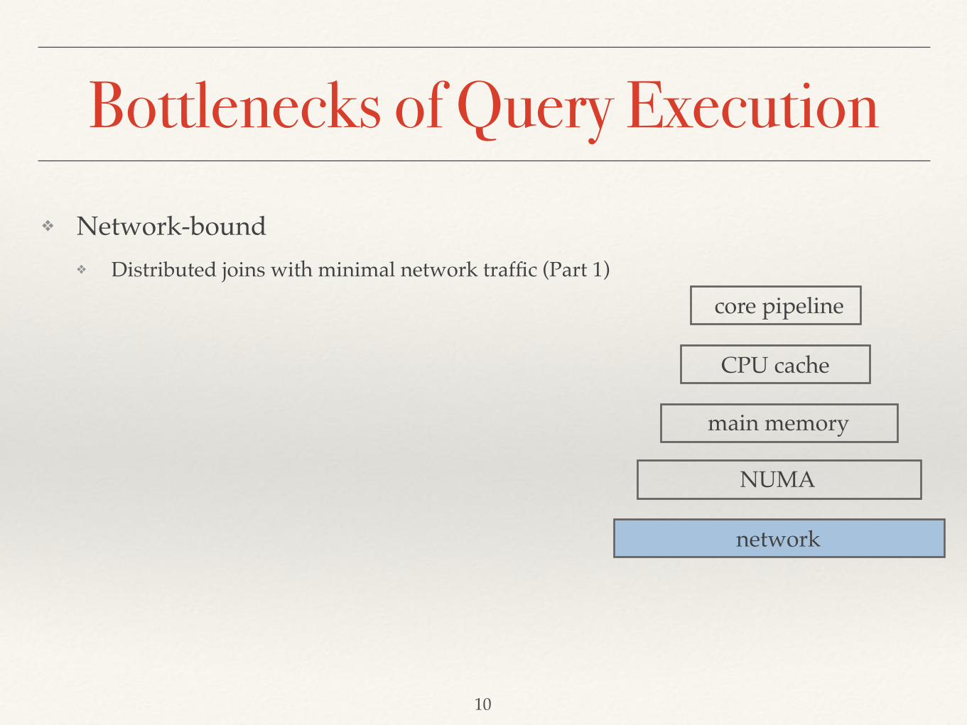
Bottlenecks of Query Execution❖ Network-bound
❖ Distributed joins with minimal network traffic (Part 1)
10
core pipeline
CPU cache
main memory
NUMA
network

❖ Network-bound❖ Distributed joins with minimal network traffic (Part 1)
❖ Memory-bound (random access)❖ (Cache-RAM-NUMA)-aware partitioning (Part 2)
11
core pipeline
CPU cache
main memory
NUMA
network
Bottlenecks of Query Execution

❖ Network-bound❖ Distributed joins with minimal network traffic (Part 1)
❖ Memory-bound (random access)❖ (Cache-RAM-NUMA)-aware partitioning (Part 2)
❖ Memory-bound (sequential access)❖ Lightweight in-memory compression (Part 3)
12
core pipeline
CPU cache
main memory
NUMA
network
Bottlenecks of Query Execution

❖ Network-bound❖ Distributed joins with minimal network traffic (Part 1)
❖ Memory-bound (random access)❖ (Cache-RAM-NUMA)-aware partitioning (Part 2)
❖ Memory-bound (sequential access)❖ Lightweight in-memory compression (Part 3)
❖ Compute-bound❖ Advanced SIMD vectorization techniques (Part 4)
13
core pipeline
CPU cache
main memory
NUMA
network
Bottlenecks of Query Execution

Part 1: Network-bound
14
CPU CPU
CPUCPU
RAM
RAM RAM
RAM
ServerServer Server
X
Server
Network
Core Core
CoreCore
core pipeline
CPU cache
main memory
NUMA
network

Network << RAM
15
❖ Network is slower than RAM❖ 4-channel DDR4 x4 = ~200 GB/s
❖ FDR InfiniBand 4X = ~5 GB/s
❖ Optimize for network traffic❖ Joins are dominant
❖ Disk hash join ~ network hash join
❖ Our contribution: track join
Band
wid
th
(GB/
sec)
04080
120160200
2-ch
anne
l DD
R4 x
1
4-ch
anne
l DD
R4 x
1
4-ch
anne
l DD
R4 x
4 012345
10 G
bit E
ther
net
QD
R In
finiB
and
4X
FDR
Infin
iBan
d 4X

Previous Work: Broadcast Join
R
S
1 2 3 4Network Nodes
Inpu
t Re
latio
ns
❖ Good if one table is small
❖ Bad for large number of nodes
16
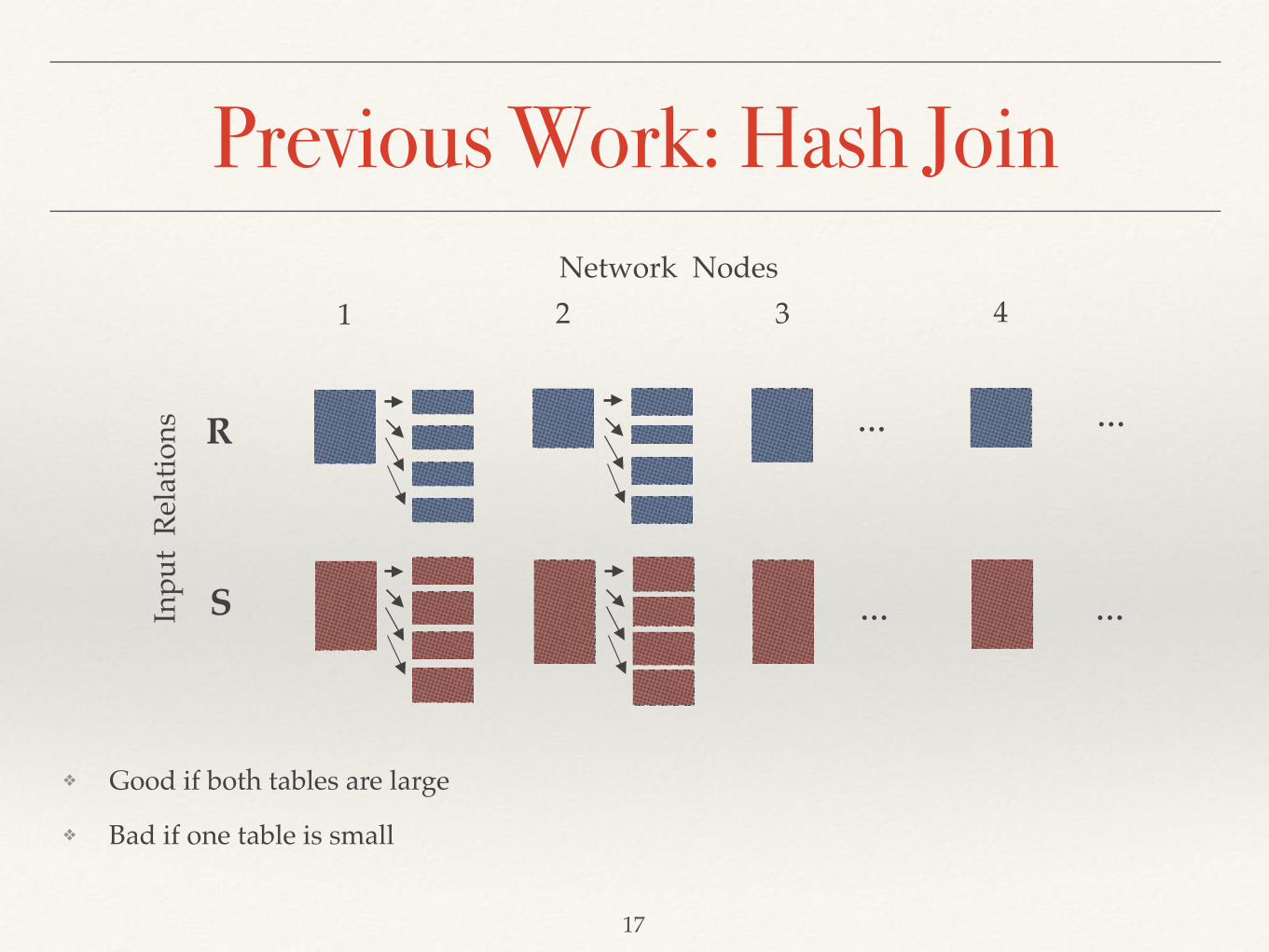
Previous Work: Hash Join
R
S
1 2 3 4
…
…
…
…Inpu
t Re
latio
ns
❖ Good if both tables are large
❖ Bad if one table is small
17
Network Nodes

Track Join: Minimize Network Traffic❖ Basic idea
❖ Logical decomposition into Cartesian product joins
❖ Optimize the transfers for each Cartesian product
❖ Basic steps❖ Track tuple locations per unique join key
❖ Generate optimal transfer schedule per key
❖ Transfer data and execute join
❖ Multiple variants❖ 2-phase, 3-phase, 4-phase
18

Track Join
R
S
Network Nodes
1 2 3 4
…
…
…
…
…
…
Hash partition unique keys
Inpu
t Re
latio
ns
19
❖ Tracking phase❖ Like a hash join of keys only

Track Join (2-phase)
20
21 3 4
1 2 3 4
key=Xnodes=[1,3,4]
R tuples(key=X)
R
S
Network NodesIn
put
Rela
tions
❖ Selective broadcast❖ On locations that have at least one tuple
R tuples(key=X)
R tuples(key=X)

Hash Join & Track Join❖ Hash Join (network cost = 10)
21
❖ 3-phase Track Join (network cost = 8)
❖ 2-phase Track Join (network cost = 12)
…""""""""""""""""""""""""""""""…"R" 2 0 4 0 0
…""""""""""""""""""""""""""""""…"S" 0 3 0 1 0
…""""""""""""""""""""""""""""""…"2 0 4 0 0
…""""""""""""""""""""""""""""""…"0 3 0 1 0
…""""""""""""""""""""""""""""""…"2 0 4 0 0
…""""""""""""""""""""""""""""""…"0 3 0 1 0
…""""""""""""""""""""""""""""""…"2 0 4 0 0
…""""""""""""""""""""""""""""""…"0 3 0 1 0
❖ 4-phase Track Join (network cost = 6)
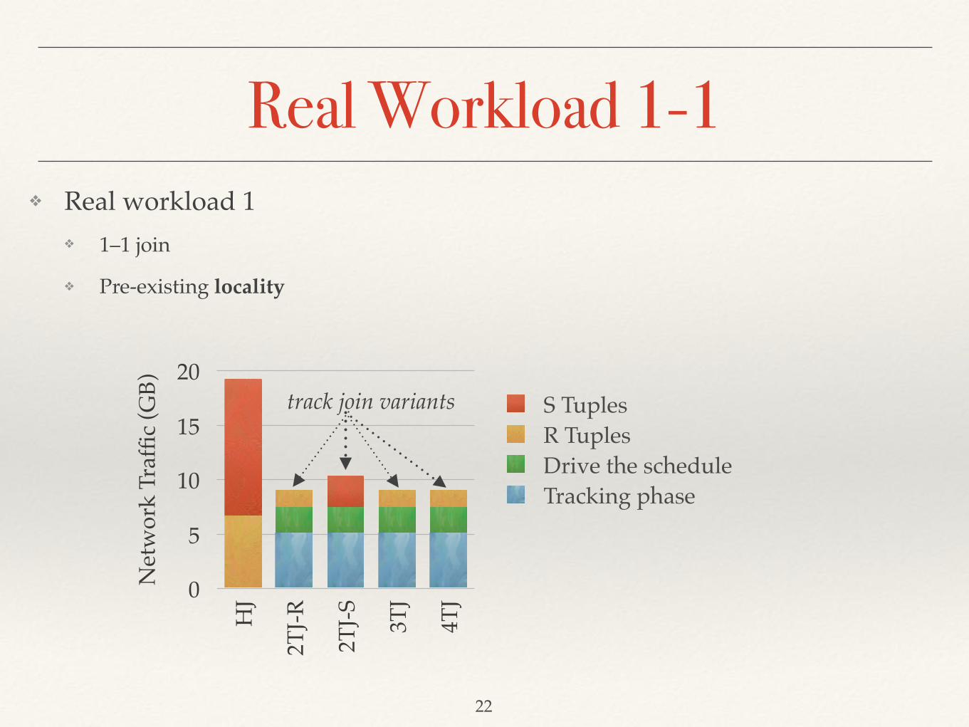
Real Workload 1-1❖ Real workload 1
❖ 1–1 join
❖ Pre-existing locality
22
Net
wor
k Tr
affic
(GB)
0
5
10
15
20
HJ
2TJ-R
2TJ-S 3T
J
4TJ
Tracking phaseDrive the scheduleR TuplesS Tuplestrack join variants

Real Workload M-N❖ Real workload 2
❖ M—N join i.e., output = ~5X inputs
❖ Pre-existing locality
23
Net
wor
k Tr
affic
(GB)
0
10
20
30
40
HJ
2TJ-R
2TJ-S 3T
J
4TJ
Tracking phaseDrive the scheduleR TuplesS Tuples
broadcasts large table
insignificant tracking cost
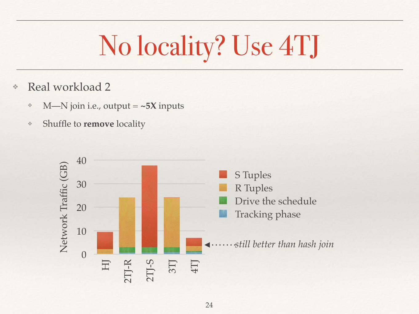
No locality? Use 4TJ❖ Real workload 2
❖ M—N join i.e., output = ~5X inputs
❖ Shuffle to remove locality
24
Net
wor
k Tr
affic
(GB)
0
10
20
30
40
HJ
2TJ-R
2TJ-S 3T
J
4TJ
Tracking phaseDrive the scheduleR TuplesS Tuples
still better than hash join

CPU+Network Time❖ Non-pipelined implementation
❖ 4 servers x 2 CPUs/sever x 4 cores/CPU x 2 threads/core
❖ 10 Gbit Ethernet projected from 1 Gbit (Columbia CLIC lab)
25
0
2
4
6
HJ
2TJ
3TJ
4TJ
Network CPU
slightly higher CPU time
much lower network time

Part 2: Memory-bound (random)
26
CPU CPU
CPUCPU
RAM
RAM RAM
RAM
ServerServer Server
X
Server
Network
Core Core
CoreCore
core pipeline
CPU cache
main memory
NUMA
network

Why partitioning?
❖ Random accesses << sequential accesses❖ Cache misses
❖ TLB misses
❖ Where to use partitioning❖ Sorting
❖ Joins
❖ Group-by aggregation
❖ Materialization
27

28
radix
hash
partition
in-cache
non-in-place
out-of-cache
in-place
in-cache
shared
shared-nothing
NUMAoblivious
previously known
Variants of Partitioning

29
radix
hash
range partition
in-cache
non-in-place
out-of-cache
out-of-cache
in-place
in-cache
shared
inblocklists
insegments
sharedshared-nothing
NUMAoblivious
NUMAaware
previously known
our contributions
Variants of Partitioning

Previous Work: Partitioning small arrays
❖ Compute histogram❖ Contiguous arrays
❖ Prefix sum of histogram
❖ Shuffle the data❖ Copy from input to output
30
input output
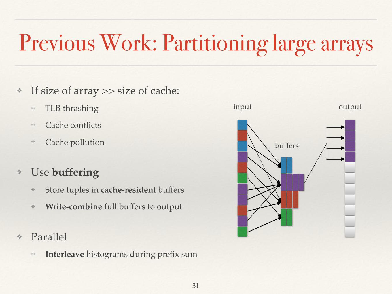
Previous Work: Partitioning large arrays
❖ If size of array >> size of cache:❖ TLB thrashing
❖ Cache conflicts
❖ Cache pollution
❖ Use buffering❖ Store tuples in cache-resident buffers
❖ Write-combine full buffers to output
❖ Parallel❖ Interleave histograms during prefix sum
31
input output
buffers

Partitioning large arrays in place
32
…
…
…
…
❖ Transfer data in cache lines❖ Amortize out-of-cache accesses
❖ RAM <—> CPU cache
❖ “Work” on the cached buffers❖ Similar to in-cache (“swap cycles”)
❖ Data transferred across buffers
❖ Recycle buffers when done❖ Flush buffer when filled
❖ Refill buffer with next data
buffers
input &output

Partitioning large arrays
33
Billi
on tu
ples
per
seco
nd
0
1
2
3
4
5
6
7
Partitioning fanout
2 4 8 16 32 64 128
256
512
1024
2048
4096
8192
non-in-place out-of-cachein-place out-of-cachenon-in-place in-cachein-place in-cache
256 partitions at RAM bandwidth
most efficient fanout5X and 3X speedup
TLB capacity

Parallel partitioning in-place
34
❖ Swap tuples in-place❖ Using atomics
❖ Extreme synchronization cost
❖ Swap blocks of tuples in-place❖ Partition to list of blocks in-place
❖ Swap blocks of tuples
❖ Amortize synchronization cost
partitionin blocks
swapblocks

Partitioning Function
❖ Radix❖ Trivial
❖ Hash❖ Depends on hash function
❖ Range❖ Slow with binary search
❖ Fast with range index
35
Billi
on tu
ples
per
seco
nd
0
5
10
15
20
25
30
35
Partitioning fanout
128
200
256
360
512
1000
1024
1800
2048
range (SIMD index)range (binary search)radixhash
RAM bandwidth for hash and radix
5X by range index

Large-scale Sorting❖ Stable LSB radix-sort
❖ Parallel radix partitioning (not in-place)
❖ In-place MSB radix-sort❖ Parallel in-place radix partitioning
❖ In-place radix partitioning
❖ Comparison-sort (CMP)❖ Parallel range partitioning (not in-place)
❖ SIMD comb-sort in the cache
36
Billi
on tu
ples
per
seco
nd
0
0.2
0.4
0.6
0.8
Billion tuples(32-bit key & payload)
1 2.5 5 10 25 50
LSB MSB CMP

NUMA Awareness
37
Tim
e (s
econ
ds)
0
10
20
30
40
50
60
70
32-bit
64-bit
NUMA awareNUMA oblivious
❖ Optimize for NUMA❖ Use local RAM per CPU
❖ Minimize NUMA transfers
❖ Transfers per sorting variant❖ LSB: up to 1 transfer
❖ MSB: up to 2 transfers
❖ CMP: up to 1 transfer
23%
53%

38
CPU CPU
CPUCPU
RAM
RAM RAM
RAM
ServerServer Server
X
Server
Network
Core Core
CoreCore
core pipeline
CPU cache
main memory
NUMA
network
Part 3: Memory-bound (sequential)

❖ Why compress?❖ Make dataset RAM resident
❖ Process data faster than RAM bandwidth
❖ Dictionary encoding❖ Process without decompressing
39
ACABADCB
ABCD
02010321
02010321
dictionary
mapping
originaldata
bitpacking
Compression in Databases

Bit Packing Layouts❖ Horizontal Bit Packing
40
❖ Vertical Bit Packing
00010101 00110001 11110101 01100110 00100100
00010000 10100000 11000000 11111000 01010000 11001000 10001000 00100000
00010000 10100000 11000000 11111000 01010000 11001000 10001000 00100000
01110110 00111100 01010001 10011000 00010110
b = 5k = 8
b = 5
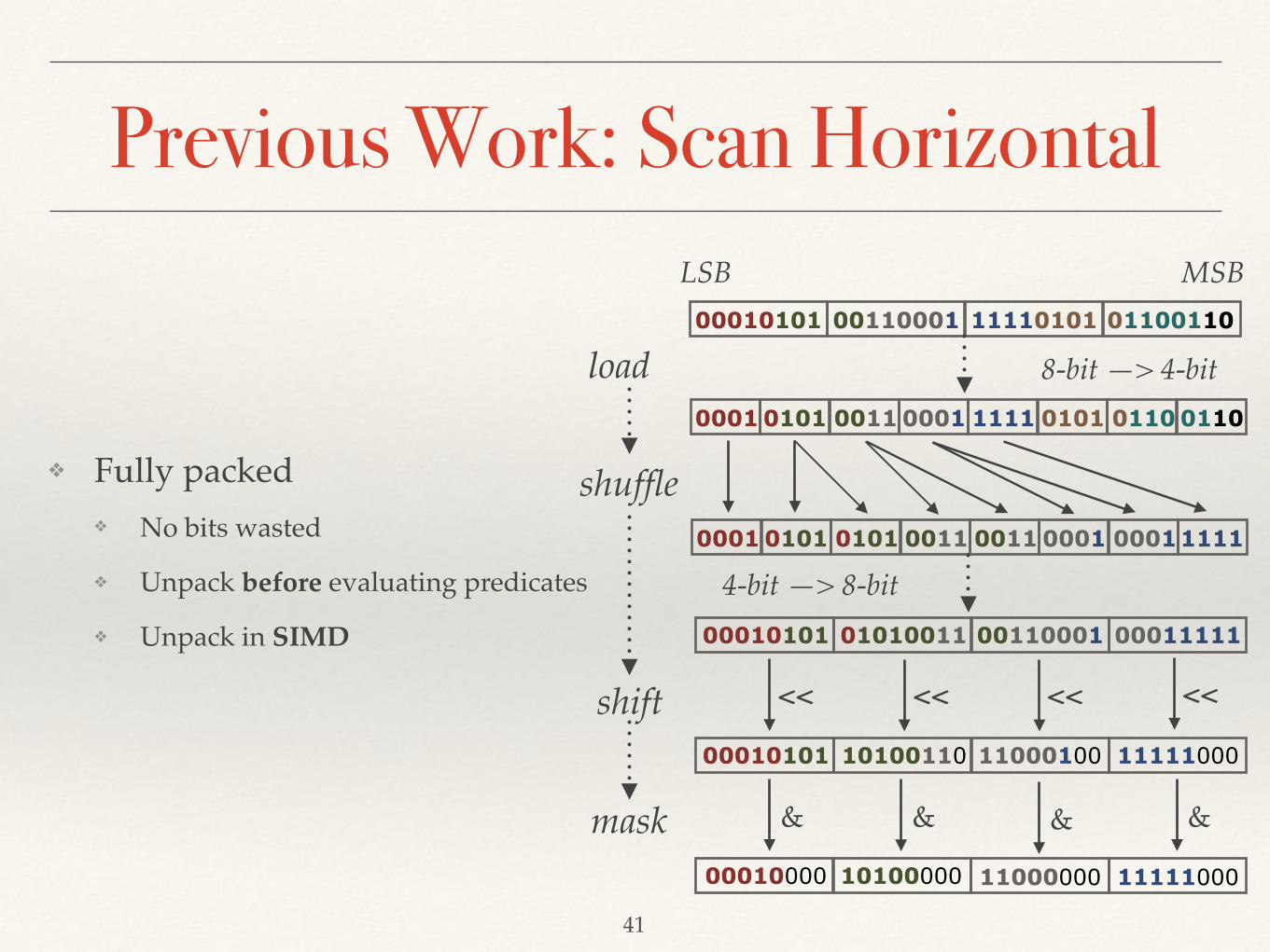
Previous Work: Scan Horizontal
41
00010101 00110001 0110011011110101
0001 0101 0011 0001 1111 0101 0110 0110
0001 0101 0101 0011 0011 0001 00011111
00010101 01010011 00110001 00011111
00010101 10100110 11000100 11111000
00010000 10100000 11000000 11111000
LSB MSB
shuffle
shift
mask
<< << << <<
8-bit —> 4-bit
4-bit —> 8-bit
& & & &
load
❖ Fully packed❖ No bits wasted
❖ Unpack before evaluating predicates
❖ Unpack in SIMD

Previous Work: Scan Horizontal
42
select … where column < C …
010 100 00 ^ 110 110 00 = 100 010 00
010 010 00
01
100 010 00 + 010 010 00 = 110 001 00
invert code
set constant C
add constant C
extract bits110 001 00 —> 01
❖ Word aligned❖ Scan without unpacking
❖ Using scalar code
❖ Bits wasted
❖ Parallel bit extraction
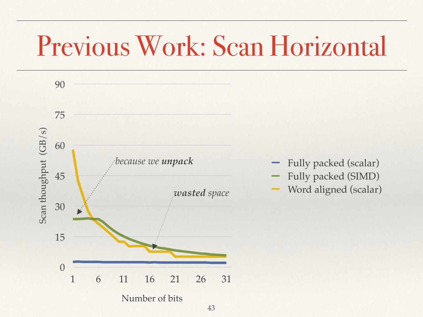
Previous Work: Scan Horizontal
43
Scan
thou
ghpu
t (G
B/s)
0
15
30
45
60
75
90
Number of bits
1 6 11 16 21 26 31
Fully packed (scalar)Fully packed (SIMD)Word aligned (scalar)wasted space
because we unpack
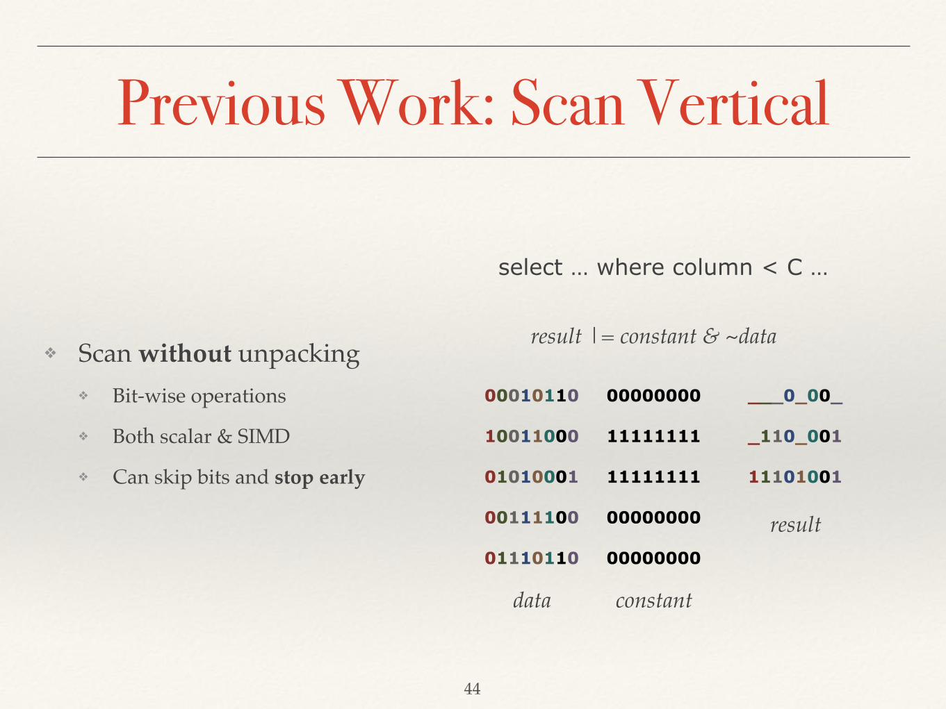
Previous Work: Scan Vertical
❖ Scan without unpacking❖ Bit-wise operations
❖ Both scalar & SIMD
❖ Can skip bits and stop early
44
00010110
10011000
01010001
00111100
01110110
00000000
11111111
11111111
00000000
00000000
___0_00_
_110_001
11101001
result |= constant & ~data
data constant
result
select … where column < C …

Previous Work: Scan Vertical
45
Scan
ning
thou
ghpu
t (G
B/s)
0
10
20
30
40
50
60
70
80
90
Number of bits
1 6 11 16 21 26 31
Vertical (k = 64)Horizontal (full)Horizontal (word)Vertical (k = 8192)
2X throughput for large k(k: number of interleaved codes)
vertical scanwithout unpacking

Pack Vertical Layout
46
pack
extract & shift
00010110
0010 0100 1000 1111 10101001 0001 0100
0001 0010 0100 0111 0101 0100 0000 0010
0000 0001 0010 0011 0010 0010 0000 0001
10011000
0000 0000 0001 0001 0001 0001 0000 0000
01010001
00111100
00000010 00010100 00011000 00011111
00001010 00011001 00010001 00000100
0000 0001 0001 0001 0000 0001 0001 0000
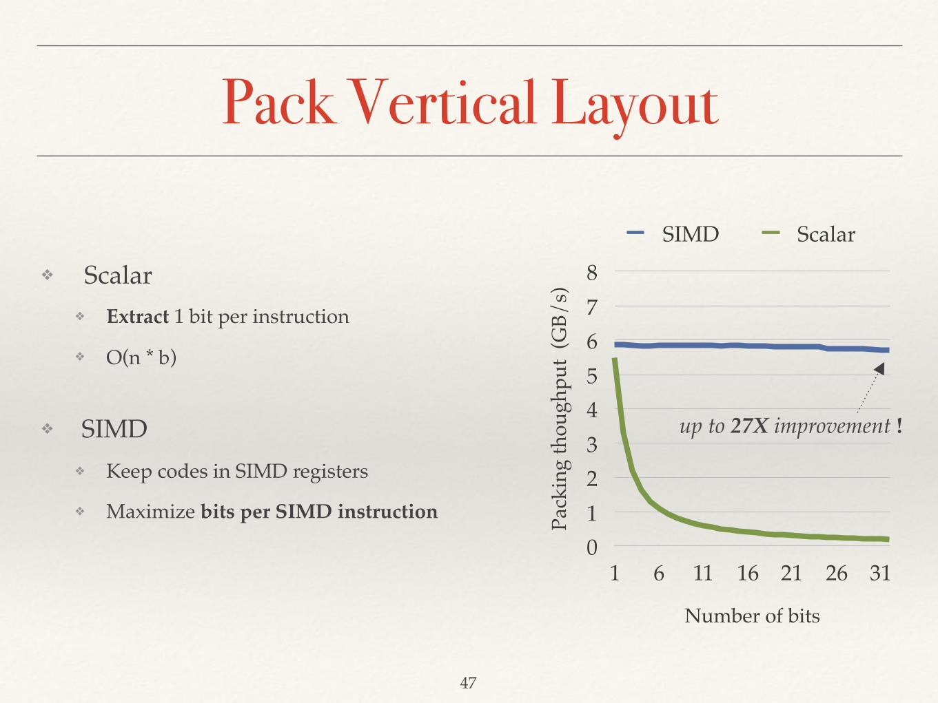
❖ Scalar❖ Extract 1 bit per instruction
❖ O(n * b)
❖ SIMD❖ Keep codes in SIMD registers
❖ Maximize bits per SIMD instruction
shift& pack
Pack Vertical Layout
47
Pack
ing
thou
ghpu
t (G
B/s)
012345678
Number of bits
1 6 11 16 21 26 31
SIMD Scalar
up to 27X improvement !
❖ Scalar❖ Extract 1 bit per instruction
❖ O(n * b)
❖ SIMD❖ Keep codes in SIMD registers
❖ Maximize bits per SIMD instruction

48
Unp
acki
ng th
ough
put
(GB/
s)
[loga
rithm
ic sc
ale]
0.1
1
10
100
Number of bits
1 6 11 16 21 26 31
SIMD Scalar
11–20X improvement !
Unpack Vertical Layout
❖ Scalar❖ Insert 1 bit per instruction
❖ O(n * b)
❖ SIMD❖ Keep codes in SIMD registers
❖ Maximize bits per SIMD instruction

What if not memory-bound?
49
❖ Using 1 thread
Scan
ning
thou
ghpu
t (G
B/s)
[loga
rithm
ic sc
ale]
0.1
1
10
100
Number of bits
1 6 11 16 21 26 31 1 6 11 16 21 26 31
Vertical (k = 8192) Horizontal fullHorizontal word Uncompressed
Multi-threaded Single-threaded
uncompressed (in SIMD)is equally fast !
compressed is faster

50
CPU CPU
CPUCPU
RAM
RAM RAM
RAM
ServerServer Server
X
Server
Network
Core Core
CoreCore
core pipeline
CPU cache
main memory
NUMA
network
Part 4: Compute-bound

Many-Core (MIC) Platforms
51
CoreL2
Cor
eL2
Cor
eL2
CoreC
oreC
oreL2
L2L2
Ring
Bus
Ring Bus~ 60 cores
❖ Mainstream CPUs❖ Aggressively out-of-order
❖ Massively super-scalar
❖ ~20 cores ($$$$)
❖ Many-core co-processors❖ 1st generation
❖ In-order
❖ Not super-scalar
❖ 16 GB of fast RAM
❖ ~60 cores

Advanced SIMD Vectorization
❖ Baseline operator❖ O(f(n)) complexity in scalar code
❖ Fully vectorized❖ O(f(n) / W) complexity in SIMD code
❖ Excluding random memory accesses
❖ Reusable vectorization techniques❖ Reuse fundamental operations
52
8-way SIMD permutation
51 1 2 3 8 13 21
71 3 2 0
215 13 1 3 2 18
45 6

Fundamental Operations
53
A B C Dvector
0 1 0 mask1
B Carray
X Y
0 1 0
A X Y D
array
mask
(output) vector
1
A B C D(input) vector
❖ Selective load
❖ Selective store
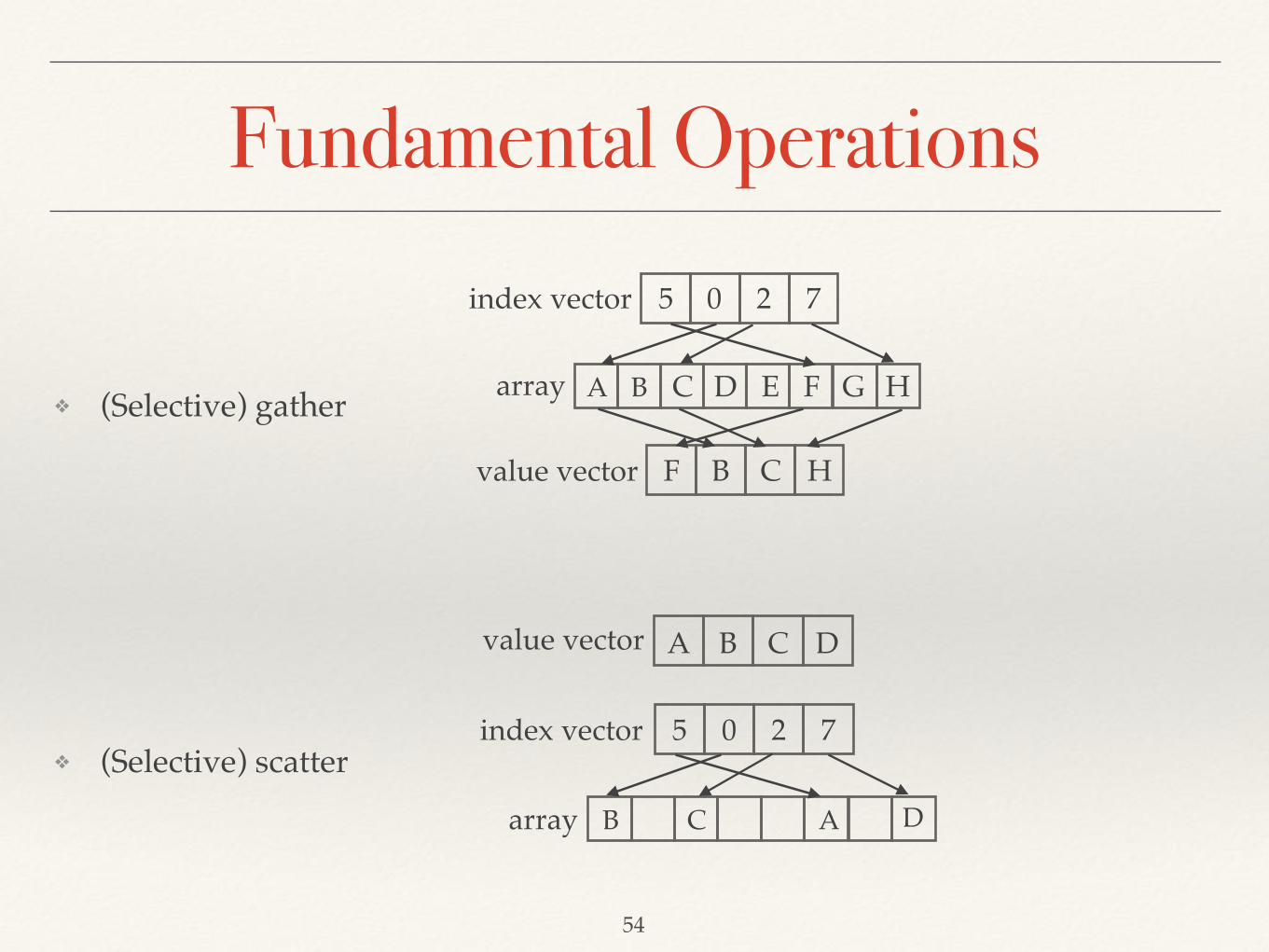
Fundamental Operations
54
❖ (Selective) gather
❖ (Selective) scatter
A B
F B C H
5 0 2 7
C D E F G H
index vector
value vector
array
B
A B C D
5 0 2 7
C A D
value vector
index vector
array
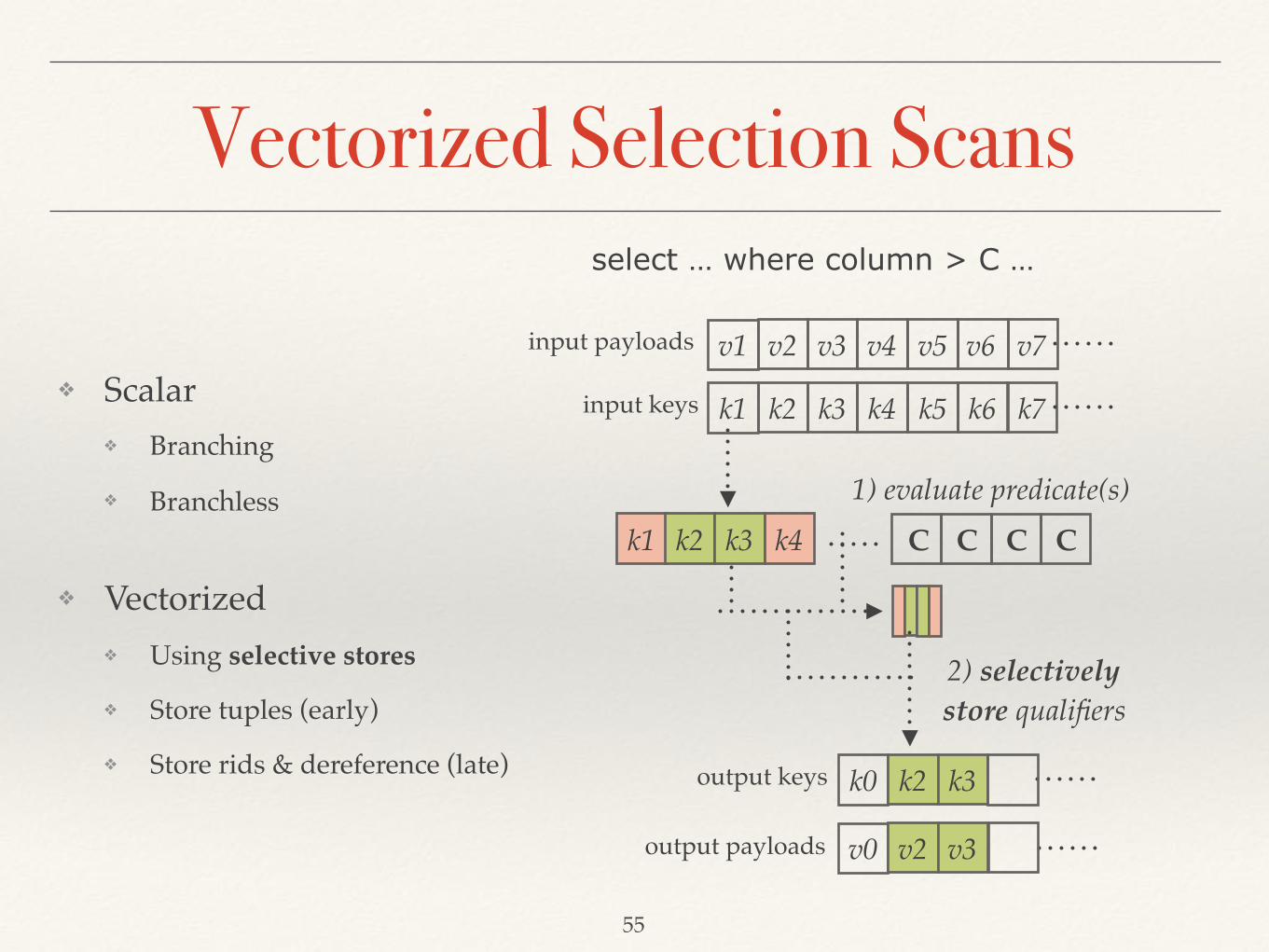
Vectorized Selection Scans
❖ Scalar❖ Branching
❖ Branchless
❖ Vectorized❖ Using selective stores
❖ Store tuples (early)
❖ Store rids & dereference (late)
55
1) evaluate predicate(s)k1 k2 k3 k4
v0 v2 v3
k0 k2 k3output keys
input payloads
input keys
2) selectivelystore qualifiers
k1 k2 k3 k4 k5 k6 k7
v1 v2 v3 v4 v5 v6 v7
C C C C
output payloads
select … where column > C …

Vectorized Selection Scans
56
Thro
ughp
ut
(bill
ion
tupl
es /
seco
nd)
0
10
20
30
40
50
Selectivity (%)
0 1 2 5 10 20 50 100
Scalar (branching)Scalar (branchless)Vectorized (early)Vectorized (late)
“late” is good for low selectivity
big speedup overall

Previous Work: Vectorized Hash Probing
❖ Scalar❖ 1 input key at a time
❖ 1 table key per input key
❖ Horizontal vectorization❖ 1 input keys at a time
❖ W table keys per input key
57
k
h
input key
hashindex
k k k k
keys
payloads
linear probing bucketized hash table
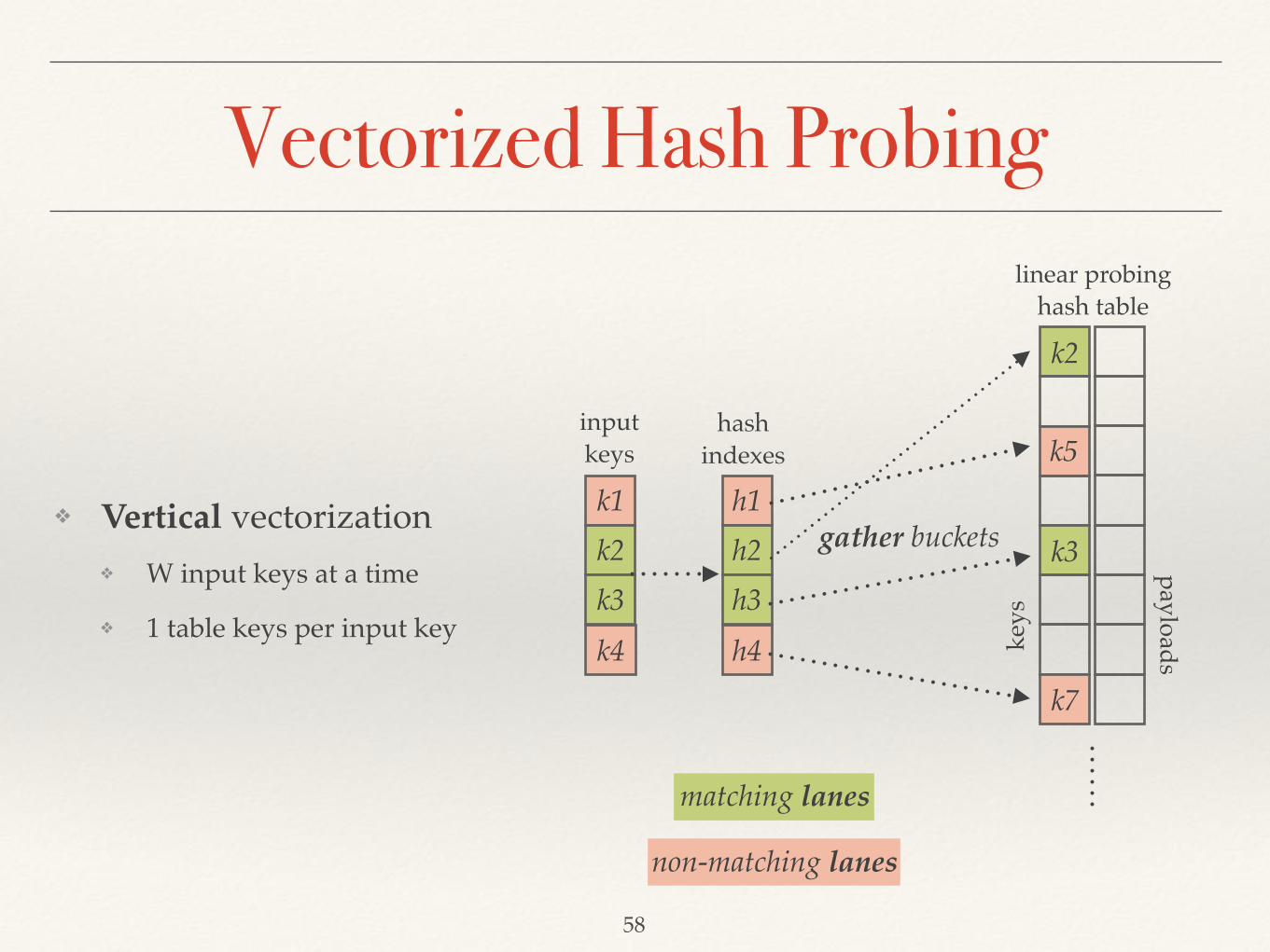
Vectorized Hash Probing
k2
k1k2k3k4
h1h2h3h4 ke
ys
payloads
inputkeys
gather buckets
k5
k7
k3
hashindexes
linear probinghash table
matching lanes
non-matching lanes
❖ Vertical vectorization❖ W input keys at a time
❖ 1 table keys per input key
58

Vectorized Hash Probing
k1k5k6k4 h1+1
h6h6
inputkeys
hashindexes
selectively load input keys
h5
0110
linear probingoffsets
linear probinghash table
h4+1
k2
k3
k7
k5
matching lanes replaced
non-matching lanes kept
59
❖ Vertical vectorization❖ W input keys at a time
❖ 1 table keys per input key

Vectorized Hash Table Probing
60
Prob
ing
thro
ughp
ut
(bill
ion
tupl
es /
seco
nd)
0
2
4
6
8
10
12
4 K
B
16
KB
64
KB
256
KB
1 M
B
4 M
B
16
MB
64
MB
ScalarVectorized (horizontal)Vectorized (vertical)
much faster in the cache !
out of the cache

Vectorized Data Shuffling
61
h1 h2 h3 h4
l1 l3
partition ids
offset array
l2
keys
k1 k2 k3 k4
1) gather offsets
l1 l2 l3 l4
k1 k3
v1 v3
output keys
k4
v4output payloads
conflicting lanes non-conflicting lanes
2) scatter tuplespartition offsets
❖ Scalar❖ Move 1 tuple at a time
❖ Vectorized❖ Scatter tuples to output
❖ Serialize conflicts

Vectorized Data Shuffling
62
h1 h2 h3 h4
l1 l3
partition ids
offset array
l2
keys
k1 k2 k3 k4
1) gather offsets
3) scatter tuplesl1 l2 l3 l4
k1 k3
v1 v3
output keys
partition offsets
output payloads
conflicting lanes non-conflicting lanes
0 0 0 1 +
k2 k4
v4v2
serialization offsets 2) serialize conflicts
❖ Scalar❖ Move 1 tuple at a time
❖ Vectorized❖ Scatter tuples to output
❖ Serialize conflicts
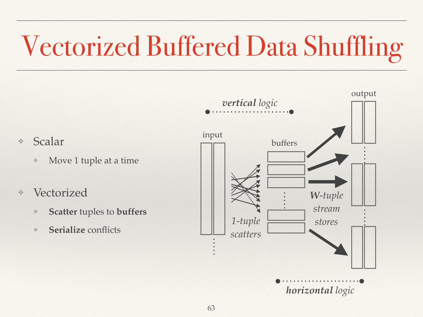
Vectorized Buffered Data Shuffling
63
1-tuplescatters
W-tuplestreamstores
inputbuffers
outputvertical logic
horizontal logic
❖ Scalar❖ Move 1 tuple at a time
❖ Vectorized❖ Scatter tuples to buffers
❖ Serialize conflicts

Vectorized Partitioning
64
Shuf
fling
thro
ughp
ut
(bill
ion
tupl
es /
seco
nd)
0
1
2
3
4
5
6
Fanout (log)
3 4 5 6 7 8 9 10 11 12 13
Scalar unbufferedScalar bufferedVector unbufferedVector buffered
vectorization orthogonal to
buffering

Vectorized Operators❖ Selection scans❖ Partitioning
❖ Histogram
❖ Data shuffling
❖ Hash table building & probing❖ Linear probing
❖ Double hashing
❖ Cuckoo hashing
❖ Bloom filter probing❖ Regular expression matching
65
❖ Sorting❖ LSB radix-sort
❖ Hash joins❖ Non-partitioned
❖ Partitioned

Hash Join Performance
66
partitionednot partitioned
Join
tim
e (s
econ
ds)
0
0.5
1
1.5
2
Scalar Vector Scalar Vector
PartitionBuild (out of cache)Probe (out of cache)Build & Probe (in cache)
not improvedimproved
3.4X !
❖ Hash join 200 with 200 million tuples (2X 32-bit key & payload)
❖ Being cache-conscious matters !

67
CPU CPU
CPUCPU
RAM
RAM RAM
RAM
ServerServer Server
X
Server
Network
Core Core
CoreCore
core pipeline
CPU cache
main memory
NUMA
network
Part 5: An Engine for Many-Cores

Why many-core CPUs?
❖ More complex cores❖ Super-scalar out-of-order cores
❖ Core size: 1st-gen << 2nd-gen << mainstream
❖ Additional layer of on-chip MCDRAM❖ ~4X higher bandwidth than DDR4 DRAM
❖ Larger than the caches (16 GB)
❖ Advanced SIMD: AVX-512❖ Same as upcoming mainstream CPUs
68
core pipeline
CPU cache
off-chip memory
NUMA
network
on-chip memory
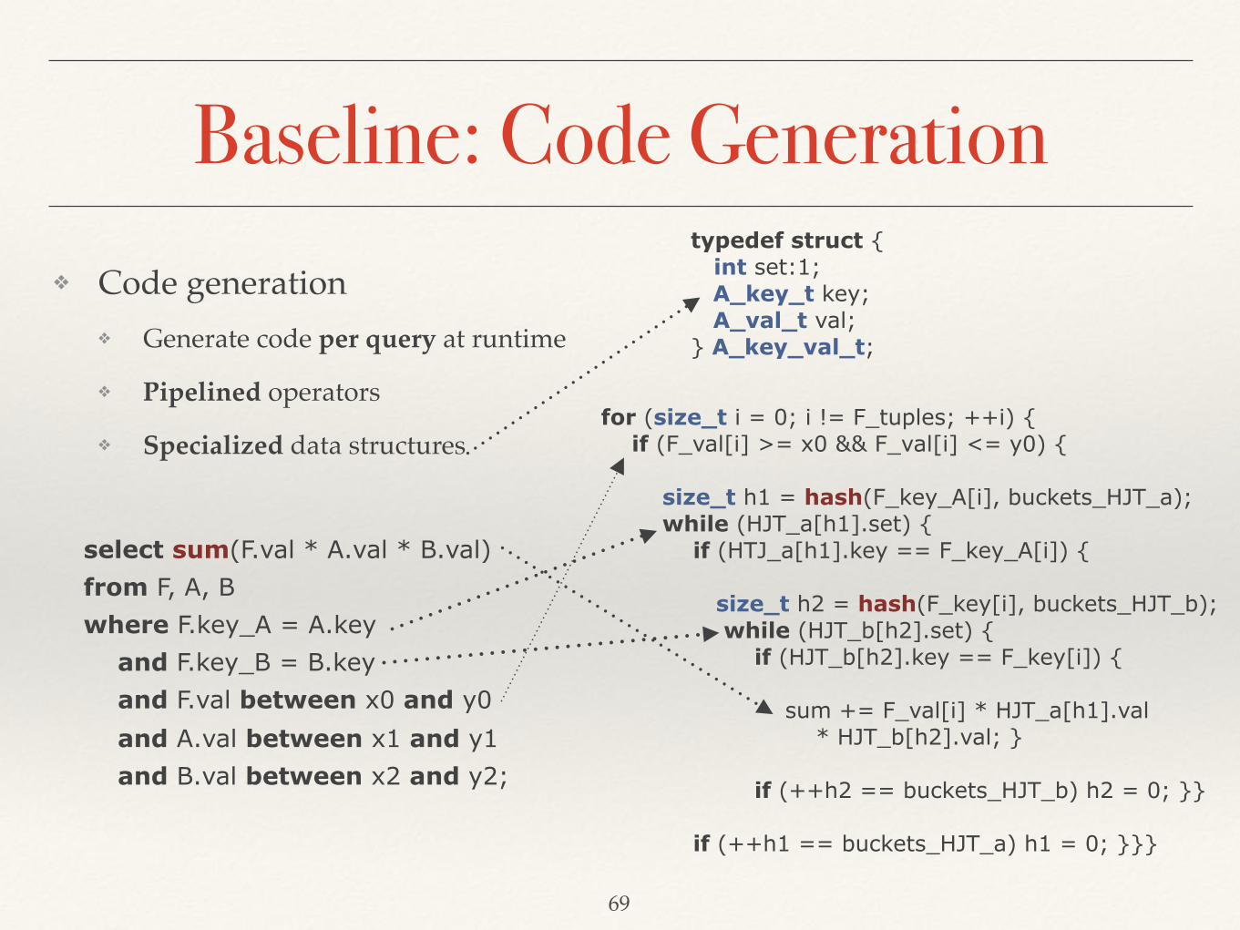
Baseline: Code Generation❖ Code generation
❖ Generate code per query at runtime
❖ Pipelined operators
❖ Specialized data structures
69
for (size_t i = 0; i != F_tuples; ++i) { if (F_val[i] >= x0 && F_val[i] <= y0) {
size_t h1 = hash(F_key_A[i], buckets_HJT_a); while (HJT_a[h1].set) { if (HTJ_a[h1].key == F_key_A[i]) {
size_t h2 = hash(F_key[i], buckets_HJT_b); while (HJT_b[h2].set) { if (HJT_b[h2].key == F_key[i]) {
sum += F_val[i] * HJT_a[h1].val * HJT_b[h2].val; }
if (++h2 == buckets_HJT_b) h2 = 0; }}
if (++h1 == buckets_HJT_a) h1 = 0; }}}
select sum(F.val * A.val * B.val) from F, A, B where F.key_A = A.key and F.key_B = B.key and F.val between x0 and y0 and A.val between x1 and y1 and B.val between x2 and y2;
typedef struct { int set:1; A_key_t key; A_val_t val;} A_key_val_t;

Baseline + SIMD Vectorization
70
❖ Maximize data parallelism❖ Written entirely in SIMD
❖ No register-resident execution
❖ Move data in cache-resident buffers
❖ SIMD can hurt performance❖ Due to cache & TLB misses
❖ Fast RAM does not help
Tim
e (in
seco
nds)
0
0.2
0.4
0.6
0.8
1
HBW LBW HBW LBW
ScalarVector
mostly hash probeSIMD <20% faster
10% selectivity 90% selectivity
mostly selection scanSIMD 2.5X faster

VIP Engine
❖ Based on “sub-operators” that …❖ Process a block of tuples at a time
❖ Process one column at a time within that block
❖ Designed to be data-parallel
❖ Implemented entirely in SIMD
❖ Why is the design fast ?❖ Specialized sub-operators can be extremely optimized
❖ Block at a time execution reduces materialization & interpretation cost
❖ Use cache-conscious execution to utilize both SIMD and fast RAM
71

❖ Hash a composite key <A, B> (of types X, Y)❖ Hash one block at a time
❖ Hash one column at a time per block
❖ Call hash_X() on column A of type X for a block of tuples
❖ Call hash_Y() on column B of type Y for a block of tuples
❖ Keep working set (block of hash values) cache-resident
❖ Amortize interpretation cost
72
void hash_int32(const int32_t* data, uint32_t* hash, size_t tuples);
Sub-operators: An Example
32-bit integer prototype

Selection Scans in VIP
❖ Based on sub-operators❖ Combine results using bitmaps
❖ Skip tuples already determined
❖ Process W items in SIMD
❖ Built-in compression❖ Horizontal dictionary compression
❖ Skip tuples if determined
❖ Decompress in 5 SIMD instructions
73
select * from T where x = 9and y > 1;
x = [1, 9, 8, 9]
y = [_, 0, _, 7]
select * from T where x = 9or y > 1;
x = [1, 9, 8, 9]
y = [2, _, 1, _]
ignore or skip

Selection Scans in VIP
74
❖ From TPC-H Q19 (SF = 1000)❖ Selection on part table
❖ Neither CNF nor DNF
❖ 0.24% selectivity
❖ Skip is essential hereTh
roug
hput
(in
billi
ons
of tu
ples
per
seco
nd)
0
5
10
15
20
HBW LBW HBW LBW
Baseline VIP
uncompressed compressed
baseline iscompute-bound
VIP is not

Hash Joins in VIP❖ Partition
❖ Inner table must fit in the cache
❖ Hash join using hash values❖ Specialized data types & code
❖ Generate rids lists
❖ Evaluate predicates❖ Use rid lists to access columns
❖ Also evaluate non-equality predicates
❖ Resolve hash conflicts
75
typedef struct { uint32_t hash; int32_t rid; } join_bucket_t; void build_hashes( const uint32_t* hashes, join_bucket_t* hash_table, […]); void probe_hashes( const uint32_t* hashes, const join_bucket_t* hash_table, int32_t* inner_rids, int32_t* outer_rids, […]);

Hash Joins in VIP
76
select l_partkey, l_suppkey, o_custkey from lineitem, orderswhere l_orderkey = o_orderkey;
select l_orderkey, l_partkey, l_suppkey from lineitem, partsupp where l_partkey = ps_partkey and l_suppkey = ps_suppkey;
Thro
ughp
ut (i
n bi
llion
s of
tupl
es p
er se
cond
)
0
0.5
1
1.5
HBW LBW HBW LBW
Baseline VIP
Hash Join 1 Hash Join 2
no improvementon slow RAM
❖ From TPC-H (SF = 30)❖ Largest base tables
❖ Core joins of TPC-H
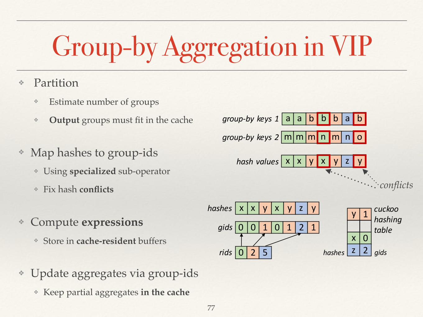
Group-by Aggregation in VIP❖ Partition
❖ Estimate number of groups
❖ Output groups must fit in the cache
❖ Map hashes to group-ids❖ Using specialized sub-operator
❖ Fix hash conflicts
❖ Compute expressions❖ Store in cache-resident buffers
❖ Update aggregates via group-ids❖ Keep partial aggregates in the cache
77
b
y
m
hashes
gids
rids
x x y x y yz
0 0 1 0 1 12
0 2 5
y 1
x 0z 2hashes gids
cuckoohashingtable
group-bykeys1
group-bykeys2
hashvalues
a a b b a
x x y x yz
m m m n on
b
conflicts
Group-by Aggregation in VIP
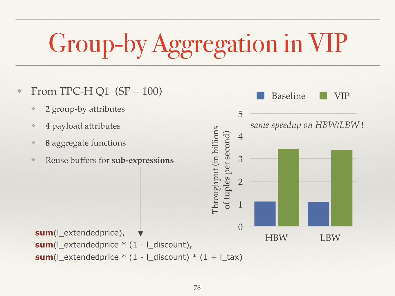
78
Thro
ughp
ut (i
n bi
llion
sof
tupl
es p
er se
cond
)0
1
2
3
4
5
HBW LBW
Baseline VIP❖ From TPC-H Q1 (SF = 100)❖ 2 group-by attributes
❖ 4 payload attributes
❖ 8 aggregate functions
❖ Reuse buffers for sub-expressions
sum(l_extendedprice), sum(l_extendedprice * (1 - l_discount), sum(l_extendedprice * (1 - l_discount) * (1 + l_tax)
same speedup on HBW/LBW !

Future Work❖ Track Join
❖ Overlap CPU & network computation to reduce end-to-end time
❖ Combine with scheduling algorithms for network transfers
❖ Compression❖ Multiple dictionaries or more complex schemes (e.g. Huffman encoding)
❖ Dynamic dictionary encoding (e.g. add & update dictionary values)
❖ Vectorization❖ Evaluate new hardware platforms with better SIMD (e.g. AVX-512)
❖ Design better hardware for database (e.g. better SIMD instructions)
❖ VIP engine❖ Pipeline operators when cache misses cannot occur
❖ Evaluate materialization strategies & build operators in VIP79

Published Papers❖ SIMD-Accelerated Regular Expression Matching
❖ At DaMoN ’16 with Eva Sitaridi, Kenneth A. Ross
❖ Rethinking SIMD Vectorization for In-Memory Databases❖ At SIGMOD ’15 with Arun Raghavan, Kenneth A. Ross
❖ Efficient Lightweight Compression Alongside Fast Scans❖ At DaMoN ’15 with Kenneth A. Ross
❖ Energy Analysis of Hardware and Software Range Partitioning❖ At TOCS with Lisa Wu, Raymond J. Barker, Martha A. Kim, Kenneth A. Ross
❖ A Comprehensive Study of Main-Memory Partitioning and its Application to Large-Scalar Comparison- and Radix-Sort
❖ At SIGMOD ’14 with Kenneth A. Ross
❖ Track Join: Distributed Joins with Minimal Network Traffic❖ At SIGMOD ’14 with Rajkumar Sen, Kenneth A. Ross
❖ Vectorized Bloom Filters for Advanced SIMD Processors❖ At DaMoN ’14 with Kenneth A. Ross
❖ High Throughput Heavy Hitter Aggregation for Modern SIMD Processors❖ At DaMoN ’14 with Kenneth A. Ross
80

Acknowledgments❖ My advisor Ken
❖ My PhD thesis committee❖ Martha, Luis, Eugene, and Stratos
❖ Friends and colleagues from the DB group❖ Fotis, John, Eva, Pablo, and Wangda
❖ Colleagues from Oracle and Amazon❖ Arun, Eric, Ippokratis, Michalis, and Raj
❖ More friends from Columbia & New York
81

Thank you!
82