PhD Thesis - School of Electrical and Computer Engineering

Measurement, Modeling, and OFDM Synchronization for the Wideband Mobile-to-Mobile Channel

A Dissertation Presented to

The Academic Faculty

By

Guillermo Acosta-Marum

In Partial Fulfillment Of the Requirements for the Degree

Doctor of Philosophy in Electrical Engineering

School of Electrical and Computer Engineering Georgia Institute of Technology

May, 2007

Copyright © 2007 by Guillermo Acosta-Marum

Measurement, Modeling, and OFDM Synchronization for the Wideband Mobile-to-Mobile Channel

Approved by: Dr. Mary Ann Ingram, Advisor School of Electrical and Computer Engineering Georgia Institute of Technology

Dr. Peter H. Rogers School of Mechanical Engineering Georgia Institute of Technology

Dr. Ye Li School of Electrical and Computer Engineering Georgia Institute of Technology

Dr. Aaron Lanterman School of Electrical and Computer Engineering Georgia Institute of Technology

Dr. Thomas G. Pratt Georgia Tech Research Institute Georgia Institute of Technology

Date Approved:

To my beautiful wife Claudia, the love of my life,

and to my son Memo, the joy of our lives.

iv

ACKNOWLEDGEMENTS

First and most importantly, I would like to thank my advisor, Dr. Mary Ann Ingram,

for trusting me and helping me achieve one of my major milestones of my life. Working

for Doctor Ingram has enriched my life not only in the academic sense. Her achieve-

ments, her work ethics, and her keen eye for every important detail have been an inspi-

ration throughout all the years I have worked with her. She has been more than a men-

tor. She has opened her arms to me and my family, and she has a very special place in

our hearts. I also want to express a very special gratitude to Dr. Thomas G. Pratt without

whom this project could have not happened.

I would also like to express my gratitude to Dr. Ye Li for all his valuable input and

comments during the time he was my co-advisor and for being part of the reading com-

mittee.

It has been a very long trip. There are so many people to thank, but I would like to

start by thanking all the people from the Consejo Nacional de Ciencia y Tecnología

(CONACYT) who had faith in me and gave me the opportunity to come back to school. I

am also very grateful to all the insitutions and companies that helped finance this project.

This project received support from the National Science Foundation (NSF), Georgia Insi-

tute of Technology, and Arinc. My special thanks to Mr. Broady Cash.

Many are the collegues who helped me through all these years. My deepest grati-

tude goes to all of them. In particular, I want to thank Dr. Weidong Xiang, Nathan Jones,

Mark Wheeler, Brett Walkenhorst, Jeng-Shiann Jiang, Kathleen Tokuda, Lu Dong, Vik-

ram Arreddi, and Anh Nguyen.

v

I want to thank my friends Roberto Uzcategui, John Gibby, and Dr. Ricardo Villalaz

for all the good conversations. Finally, my deepest love goes to my wife Claudia and my

son Memo. You have been my loyal partners in this adventure. I could not have done it

without you. I love you both.

vi

TABLE OF CONTENTS

ACKNOWLEDGEMENTS IV

LIST OF TABLES XI

LIST OF FIGURES XIII

SYMBOLS AND ABBREVIATIONS XXV

SUMMARY XXVIII

CHAPTER 1: INTRODUCTION 1

CHAPTER 2: BACKGROUND 5

2.1 Channel Modeling.............................................................................................5

2.1.1 Small Scale Fading..............................................................................5

2.1.2 Basic Model and Popular Statistics .....................................................7

2.1.3 Scattering Function..............................................................................8

2.1.4 MTM Model........................................................................................12

2.1.5 Measured MTM Doppler ....................................................................17

2.2 Channel Sounding ..........................................................................................19

2.2.1 Narrowband Sounding Techniques ...................................................20

2.2.2 Wideband Sounding Techniques.......................................................21

vii

2.2.2.1 Tone Stepping .....................................................................21

2.2.2.2 The RUSK™ Multitone System.............................................22

2.2.2.3 Periodic Pulse Sounding Method.........................................23

2.2.2.4 Pulse Compression Techniques..........................................24

2.2.2.5 Chirp Sounding....................................................................30

2.3 Channel Emulation .........................................................................................33

2.4 OFDM Synchronization Algorithms.................................................................39

2.4.1 Frame or Symbol Acquisition.............................................................40

2.4.2 Frame or Symbol Tracking ................................................................41

2.4.3 Frequency Offset Acquisition.............................................................42

2.4.4 Frequency Offset Tracking ................................................................44

2.4.5 Sampling Frequency Offset Acquisition.............................................44

CHAPTER 3: OFDM SYNCHRONIZATION 46

3.1 OFDM Synchronization Offsets ......................................................................46

3.1.1 Frequency Offset Analysis.................................................................48

3.1.2 Sampling Frequency Offset Analysis.................................................49

3.1.3 Symbol Timing Offsets Analysis ........................................................51

3.1.4 Combined Effects of Synchronization Offsets ...................................54

3.2 OFDM Offsets Estimation and Compensation................................................57

viii

CHAPTER 4: CHANNEL MEASUREMENT SYSTEMS 66

4.1 2.4 GHz Channel Sounding System Development.........................................66

4.1.1 Sounding Waveform Analysis and Processing ..................................67

4.1.1.1 Autocorrelation.....................................................................69

4.1.1.2 Spectral Estimation..............................................................73

4.1.1.3 Sampling Process................................................................81

4.1.2 Post-Collection System Testing.........................................................85

4.1.2.1 Clock Synchronization .........................................................85

4.1.2.2 Harmonic Distortion Test .....................................................89

4.1.2.3 System’s Performance.........................................................96

4.2 5.9 GHz Channel Sounding System Development.......................................104

4.2.1 System Description..........................................................................104

4.2.2 Sounding Waveform ........................................................................107

4.2.3 OFDM Sounding ..............................................................................109

4.2.4 Alias Problem...................................................................................113

CHAPTER 5: MEASUREMENT CAMPAIGNS 120

5.1 Phase One: 2.4 GHz Measurement Campaign ............................................120

5.1.1 Period One: Finding Worst-Case Delay...........................................120

5.1.2 Period Two.......................................................................................135

ix

5.2 Phase Two: 5.9 GHz Measurement Campaign ............................................136

CHAPTER 6: MEASUREMENT RESULTS AND CHANNEL MODELING 147

6.1 Phase One Channel Modeling......................................................................148

6.1.1 Statistical Model Develpment ..........................................................148

6.1.1.1 Resulting Tap Characteristics............................................148

6.1.1.2 Testing Using a DSRC Simulink™ Model..........................154

6.1.1.3 Model Validation Process ..................................................156

6.1.1.4 Model Results ....................................................................157

6.1.1.5 Statistical Model Extraction Defficiencies ..........................159

6.1.1.6 Statistical Model Conclusions ............................................165

6.1.2 Partitioned Model Development.......................................................165

6.1.2.1 BER Partitions ...................................................................166

6.1.2.2 MD Partitions .....................................................................167

6.1.2.3 Results for Phase I Techniques.........................................168

6.1.2.4 K-Factor .............................................................................173

6.2 Phase Two Channel Modeling......................................................................174

6.2.1 Methodology ....................................................................................175

6.2.2 Results for Phase II Techniques......................................................180

6.2.3 PER Test Procedure........................................................................188

x

6.2.4 Phase II Model Conclusions ............................................................190

CHAPTER 7: MODEL SUMMARIES 191

7.1 Proposed WAVE/DSRC Model.....................................................................191

7.2 Model Descriptions .......................................................................................192

7.2.1 MTM - Expressway Oncoming without Wall, 300m – 400m

Scenario...........................................................................................193

7.2.2 RTM - Urban Canyon, 100 m Scenario ...........................................196

7.2.3 RTM – Expressway, 300m – 400m Scenario ..................................201

7.2.4 MTM - Urban Canyon Oncoming, 100m Scenario...........................206

7.2.5 RTM - Suburban Street, 100m Scenario .........................................211

7.2.6 MTM - Expressway Same Direction with Wall, 300m – 400m

Scenario...........................................................................................218

CHAPTER 8: CONCLUSIONS 222

8.1 Contributions.................................................................................................222

8.2 Suggested Future Work................................................................................223

REFERENCES 226

VITA 233

xi

LIST OF TABLES

Table 1: Reference generators specifications .....................................................87

Table 2: Description of the locations for each scenario.....................................138

Table 3: 6- and 12-tap model results.................................................................150

Table 4: DSRC standard specifications.............................................................155

Table 5: Total transmitted bits, received errors, and BER for each

process................................................................................................158

Table 6: Overall 10-Tap model parameters.......................................................162

Table 7: Spectra offset correlation coefficient matrix ........................................163

Table 8: Partition by BER Criterion Results ......................................................166

Table 9: Partition by MD Results.......................................................................168

Table 10: K-factors for the BER partition model..................................................174

Table 11: MTM - Expressway Oncoming without Wall, 300m – 400m

Model...................................................................................................193

Table 12: RTM – Urban Canyon, 100 m Short Model .........................................196

Table 13: RTM – Urban Canyon, 100 m Long Model..........................................198

Table 14: RTM – Expressway, 300m – 400m 140 km/hr Model .........................201

Table 15: RTM – Expressway, 300m – 400m 200 km/hr Model .........................204

Table 16: MTM - Urban Canyon Oncoming, 100m Short Model .........................206

Table 17: MTM - Urban Canyon Oncoming, 100m Long Model..........................208

Table 18: RTM - Suburban Street, 100m Short Model........................................211

xii

Table 19: RTM - Suburban Street, 100m Long Model ........................................214

Table 20: MTM - Expressway Same Direction with Wall, 300m – 400m

Model...................................................................................................218

xiii

LIST OF FIGURES

Figure 1: Doppler spectrum for MTM and cellular channels (a=0) [63]. ...............14

Figure 2: Normalized Doppler spectrum for a mobile-to-mobile link as a

function of normalized Doppler shift for different values of the ratio

α=fd1/fd2 (coherent detection) [86]. ......................................................16

Figure 3: Normalized Doppler spectrum for a mobile-to-mobile link as a

function of normalized Doppler shift for different values of the ratio

α=fd1/fd2 (square law detection) [86]....................................................17

Figure 4: Flat-fading Doppler measurements in [48]. ...........................................18

Figure 5: Examples of Doppler spectra measured in a fixed-to-mobile

environment [91]....................................................................................19

Figure 6: First elements of transmitted and locally generated sequences

shown for three transmitted sequence repetition cycles. ......................28

Figure 7: Transmitted sequence and locally generated sequence alignment

period [81]. ............................................................................................30

Figure 8: Channel emulator setup for IEEE 802.11g throughput testing. .............34

Figure 9: Spirent TAS 4500 hardware channel emulator parameters setup:

(a) number of taps and (b) delay per tap...............................................35


(a) Doppler parameters per tap and (b) power per tap..........................35


(a) large-scale fading per tap and (b) output power adjustment............36

Figure 12: Matlab™ Simulink™ software channel models: (a) multipath

Rayleigh and (b) Rician fading. .............................................................36

xiv

Figure 13: Common synchronization structure [78]................................................40

Figure 14: Basic correlation process. .....................................................................42

Figure 15: First order approximation behavior for L=10. ........................................62

Figure 16: Second order approximation behavior for L=10. ...................................63

Figure 17: Normalized empirical cumulative distribution functions (CDF) for

the measurement error of the four synchronization offsets. Each

CDF represents approximately 600 data points. ...................................65

Figure 18: Receiver system in van to the left and transmitter system in

compact car to the right.........................................................................67

Figure 19: Possible overlapping regions. ...............................................................70

Figure 20: Simulation of (4.11) for different values of δ and 50 nscT = . ..............72

Figure 21: Direct plot of (4.13) for 100 nscT = .......................................................74

Figure 22: Detailed view of the center peak of direct plot of (4.13). .......................74

Figure 23: 511-MLS waveform simulation. .............................................................75

Figure 24: Non-averaged Power Spectrum estimation of simulated waveform

for 100 nscT = . .....................................................................................76

Figure 25: Detailed view of the center peak of Figure 24. ......................................76

Figure 26: Averaged (20 periodogram) Power Spectrum estimation of

simulated waveform for 100 nscT = . ....................................................77


Figure 28: Measured Power Spectrum for 100 nscT = ..........................................78

Figure 29: Measured detailed view ........................................................................79

xv

Figure 30: Recorded signal processing. .................................................................79

Figure 31: Non-averaged Power Spectrum estimation of the recorded

response at the output of the channel emulator with just LOS..............80

Figure 32: Averaged Power Spectrum estimation of the recorded response at

the output of the channel emulator with just LOS..................................80


Figure 34: Digital down-converter lowpass filter response for a decimation of

four. .......................................................................................................83

Figure 35: Unsynchronized IF Wired Setup............................................................88

Figure 36: Measured free running IF response with the equipment cold. ..............89

Figure 37: Two-tone LNA output with a -35 dBm TX generator output. This is

the maximum level for a clean signal. ...................................................90

Figure 38: Two-tone LNA output with a -30 dBm TX generator output.

Harmonic distortion begins....................................................................90

Figure 39: Two-tone LNA output with a -5 dBm TX generator output. LNA

output is saturated.................................................................................91

Figure 40: Two-tone LNA output with a 0 dBm TX generator output.

Harmonics level almost equals original signal.......................................91

Figure 41: Probing signal LNA output with a -30 dBm TX generator output...........92

Figure 42: Probing signal LNA output with a 0 dBm TX generator output..............93

Figure 43: Probing signal LNA output with a +5 dBm TX generator output.

Even for this output level, there are no harmonics present. ..................93

Figure 44: Probing signal LNA output with a +5 dBm TX generator output.

Notice that the span is now 1000 Hz.....................................................94

xvi

Figure 45: Probing signal downconverter IF output with a +5 dBm TX

generator output. This window size is similar to the short-time

Doppler profile. ......................................................................................95

Figure 46: Probing signal downconverter IF output with a +5 dBm TX

generator output. This window size is equal to the long-time

Doppler profile. ......................................................................................95

Figure 47: Simulated two path 50 ns resolution PDP. ............................................97

Figure 48: (a) Transmitter time scale (nTc), and (b) Receiver time scale (kTs)

[49]. .......................................................................................................98

Figure 49: Channel emulator setup. .....................................................................100

Figure 50: Channel emulator 100cT ns= PDP for first and second baud

sample and time aligned response......................................................101

Figure 51: Channel emulator 100 nscT = vs. 50 nscT = PDP’s. ........................102

Figure 52: Channel emulator 100 nscT = vs. 50 nscT = scattering functions:

(a) & (b) Isometric views, (c) & (d) delay vs. amplitude views, and

(e) & (f) frequency vs. amplitude views. ..............................................103

Figure 53: 5.9 GHz transmitter system.................................................................104

Figure 54: 5.9 GHz receiver system. ....................................................................106

Figure 55: PDP obtained using the MLS signal through a channel emulator. ......108

Figure 56: PDP obtained using the OFDM signal through the same setting in

a channel emulator. We can clearly see the improvement in time

resolution.............................................................................................108

Figure 57: Zero padded OFDM sounding signal. We can notice the impulse

magnitude reduction and the ripples surrounding it. ...........................110

xvii

Figure 58: Scattering function using an OFDM sounding signal through a

seven path channel with different maximum Doppler frequencies. .....111

Figure 59: Example of OFDM PDPs with and without calibration. .......................113

Figure 60: First tap Doppler spectrum from the same segment used in Figure

61 obtained using the OFDM section of the sounding waveform........114

Figure 61: First tap Doppler spectrum from an oncoming scenario segment

obtained using the MLS section of the sounding waveform. ...............115

Figure 62: Measured OFDM section spectrum.....................................................116

Figure 63: Combined waveform spectrum produced by the ESG E4438C

signal generator...................................................................................117

Figure 64: MLS section spectrum at the output of the ADV-3000T

downconverter.....................................................................................118

Figure 65: Correct MLS section spectrum for a 2x sampling................................119

Figure 66: MLS section spectrum used in the measurement campaign...............119

Figure 67: Berkeley-Varitronics Locust system to the left and the chosen

Linksys access point to the right. ........................................................122

Figure 68: Vehicles used with transmission antenna on van’s hood and

reception antenna on car’s trunk. ........................................................122

Figure 69: Berkeley-Varitronics Locust multipath screen. ....................................123

Figure 70: Received power for the first session. ..................................................126

Figure 71: Above threshold RMS delay spread MA with corresponding

histogram for the first session. ............................................................127

Figure 72: Location A @ (33.7487, -84.3857) I-285 exit ramp with distant

office buildings.....................................................................................127

xviii

Figure 73: Location B @ (33.7552, -84.389) Downtown Atlanta involving a

park inside an urban canyon. ..............................................................128

Figure 74: Location C @ (33.7723, -84.3872) Midtown Atlanta near the two

tallest buildings in the city. We have flat land surrounded by very

tall buildings.........................................................................................128

Figure 75: Received power for the second session..............................................129


histogram.............................................................................................129

Figure 77: Location D @ (33.7575, -84.3877) Three-way intersection in

downtown Atlanta. ...............................................................................130

Figure 78: Received power for the third session. .................................................130


histogram for the third session. ...........................................................131

Figure 80: Location E @ (33.9179, -84.3392) Another I-285 exit ramp located

close to office buildings. ......................................................................131

Figure 81: Received power for the fourth session. ...............................................132


histogram for the fourth session. .........................................................132

Figure 83: Location F @ (33.7810, -84.3937) Georgia Tech campus next to

the Alexander Memorial Coliseum and Turner Television studios

with a T-intersection with flat land near long buildings. .......................133

Figure 84: Location G @ (33.7562, -84.3008) Georgia Dome parking lot............133

Figure 85: Location G is a very complex steel structure with many tunnels

and ramps. ..........................................................................................134

Figure 86: Location H @ (33.7756, -84.3873) Georgia Tech Centergy

construction site. It is an urban canyon with parking lots. ...................134

xix

Figure 87: Phase One Period Two recorded data format.....................................135

Figure 88: Phase Two recorded data structure. ...................................................137

Figure 89: Approaching or oncoming vehicle is the white van seen on the

left........................................................................................................139

Figure 90: Roadside antenna at the intersection of Peachtree Street and

Peachtree Circle..................................................................................140

Figure 91: Signal envelope and deleted segments for the RTM – Urban

Canyon 100m scenario. The signal level corresponds to relative

power, i.e., relative to the minimum signal recorded. It does not represent RF signal power. .................................................................141

Figure 92: Roadside antenna on GA 78. ..............................................................142

Figure 93: Starting point of receiver vehicle on Edgewood Avenue. ....................143

Figure 94: Roadside antenna at the intersection of Memorial Drive and

Candler Road. .....................................................................................144

Figure 95: Signal envelope and deleted segments for the RTM – Suburban

Street 100m scenario. The signal level corresponds to relative

power, i.e., relative to the minimum signal recorded. It does not represent RF signal power. .................................................................145

Figure 96: Typical conditions for the Expressway Same Direction with Wall

scenario. The transmitter vehicle kept a 400 m separation to the

front of the receiver vehicle. ................................................................146

Figure 97: Expressway PDPs obtained using (2.37). ...........................................151

Figure 98: 6-tap model scattering function. ..........................................................151

Figure 99: 12-tap model scattering function. ........................................................152

Figure 100: Synthesized 12-tap model scattering function.....................................153

xx

Figure 101: Simulated short time Doppler spectra and long time Doppler

spectrum for the third tap of the 12-tap model scattering function. .....153

Figure 102: Measured short time Doppler spectra and long time Doppler

spectrum of a latter tap of one of the resulting scattering functions. ...154

Figure 103: Recorded channel and models CDFs using the BER per 0.7 s

segment, a 64 OFDM symbol frame, and adaptive modulation. .........158

Figure 104: Recorded channel and models CDFs using the BER measured for

each 64 OFDM symbol frame and adaptive modulation. ....................159

Figure 105: All spectra contribution for the first tap of an averaged statistical

model. The thick line represents the tap spectrum..............................161

Figure 106: All spectra contribution for the last tap of an averaged statistical

model. The thick line represents the tap spectrum..............................161

Figure 107: Overall 10-tap model without frequency adjustment scattering

function................................................................................................162

Figure 108: Frequency aligned spectra contribution for the last tap of the

overall model. The thick line represents the tap spectrum. .................164

Figure 109: Frequency aligned spectra contribution for the last tap of the

overall model. The thick line represents the tap spectrum. .................164

Figure 110: Overall 10-tap model with frequency adjustment scattering

function................................................................................................165

Figure 111: BER partition one scattering function. .................................................167

Figure 112: BER partition four scattering function..................................................167

Figure 113: Recorded channel and models CDFs using the BER per 0.7 s

segment, a 64 OFDM symbol frame, and adaptive modulation. .........170

Figure 114: Recorded channel and models CDFs using the BER measured for

each 64 OFDM symbol frame and adaptive modulation. ....................170

xxi

Figure 115: Recorded channel and BER partition model CDFs using the BER

per 0.7 s segment, a 168 OFDM symbol frame, and a fixed 6

Mbps modulation. ................................................................................172

Figure 116: Recorded channel and BER partition model CDFs using the BER

measured for each 168 OFDM symbol frame (1000, data bytes)

with fixed 6 Mbps modulation. .............................................................172

Figure 117: Suburban Expressway MTM Same Direction Wall PDPs obtained

using (2.37). ........................................................................................175

Figure 118: The overall power delay profile (PDP) for the expressway, same-

direction travel scenario. .....................................................................181

Figure 119: An example spectrum estimate for a 0.6 second segment. The flat

part indicates the level corresponding to the K-factor measured for

this segment. .......................................................................................182

Figure 120: Histogram of Rician component frequencies for Tap. No. 1................182

Figure 121: Average of the parts of the spectra that were removed by the level

and hole methods for Tap. No. 1.........................................................183

Figure 122: Histogram of Rician component frequencies for Tap No. 4.................184

Figure 123: Average of the parts of the spectra that were removed by the level

and hole methods for Tap. No. 1.........................................................184

Figure 124: Histogram of K-factor values for Tap. 1...............................................185

Figure 125: Histogram of K-factor values for Tap 4................................................186

Figure 126: Two-shape fit to the random part spectrum of Tap One......................187

Figure 127: Emulated spectrum comparison..........................................................188

Figure 128: Block diagram of the PER test setup...................................................189

xxii

Figure 129: Tap spectra for the MTM Expressway Oncoming scenario. In blue:

the measured Doppler spectrum for the random part. In red: the

composite or customized spectrum, which corresponds to Table

11. .......................................................................................................194

Figure 130: For the Expressway Oncoming 400m scenario, mean PER and

95% confidence intervals for -79 dBm 1000 Byte PSDU (top

curves), -79 dBm, 200 Byte PSDU (middle three curves), and -76

dBm 1000 Byte PSDU (bottom curves)...............................................195

Figure 131: Tap spectra for the RTM Urban Canyon 100m scenario, short

model. In blue: the measured Doppler spectrum for the random

part. In red: the composite or customized spectrum, which

corresponds to Table 12......................................................................197

Figure 132: Tap spectra for the RTM Urban Canyon 100m scenario, long




Figure 133: RTM – Urban Canyon 100m scenario: mean PER and 95%

confidence intervals for -79 dBm and 1000-Byte PSDU, short and

long models. ........................................................................................200

Figure 134: Tap spectra for the RTM Expressway 300-400m scenario. In blue:

the measured Doppler spectrum for the random part. In red: the

composite or customized spectrum, which corresponds to Table

14. .......................................................................................................202

Figure 135: RTM – Expressway 300-400m scenario: mean PER and 95%

confidence intervals for -79 dBm, for 200- and 1000-Byte PSDUs

and vehicle speed of 140 km/hr. .........................................................203

Figure 136: RTM – Expressway 300-400m scenario: mean PER and 95%

confidence intervals for -79 dBm, for 200- and 1000-Byte PSDUs

and vehicle speed of 200 km/hr. .........................................................205

xxiii

Figure 137: Tap spectra for the MTM Urban Canyon 100m scenario, short




Figure 138: Tap spectra for the MTM Urban Canyon 100m scenario, long




Figure 139: MTM – Urban Canyon 100m scenario: mean PER and 95%

confidence intervals for -79 dBm and 1000-Byte PSDU, short and

long models. ........................................................................................210

Figure 140: First four tap spectra for the RTM Suburban Street 100m scenario,

short model. In blue: the measured Doppler spectrum for the

random part. In red: the composite or customized spectrum, which


Figure 141: Second four tap spectra for the RTM Suburban Street 100m

scenario, short model. In blue: the measured Doppler spectrum for

the random part. In red: the composite or customized spectrum,

which corresponds to Table 18. ..........................................................213

Figure 142: First four tap spectra for the RTM Suburban Street 100m scenario,

long model. In blue: the measured Doppler spectrum for the

random part. In red: the composite or customized spectrum, which


Figure 143: Second four tap spectra for the RTM Suburban Street 100m

scenario, long model. In blue: the measured Doppler spectrum for

the random part. In red: the composite or customized spectrum,

which corresponds to Table 19. ..........................................................216

Figure 144: Mean PER and 95% confidence intervals for -79 dBm, 1000-Byte

PSDU, for the short and long Suburban Street RTM 100m

scenarios. ............................................................................................217

xxiv

Figure 145: First four tap spectra for the MTM Expressway Same Direction

with Wall 300-400m scenario. In blue: the measured Doppler

spectrum for the random part. In red: the composite or customized

spectrum, which corresponds to Table 20...........................................219

Figure 146: Second four tap spectra for the MTM Expressway Same Direction

with Wall 300-400m scenario. In blue: the measured Doppler

spectrum for the random part. In red: the composite or customized

spectrum, which corresponds to Table 20...........................................220

Figure 147: Resulting PER for the Expressway Same Direction scenario. ............221

xxv

SYMBOLS AND ABBREVIATIONS

ADC Analog-to-Digital Converter

AWGN Additive White Gaussian Noise

BER Bit Error Rate

BPSK Binary Phase Shift Keying

BS Base Station

BW Bandwidth

CAZAC Constant Amplitude Zero Autocorrelation

CCD Charge-Coupled Devices

CDF Cumulative Distribution Function

CIR Channel Impulse Response

DA Data Aided

DAB Digital Audio Broadcasting

DAC Digital-to-Analog Converter

DARPA Defense Advanced Research Projects Agency

DSP Digital Signal Processor

DSRC Dedicated Short Range Communications

DVB Digital Video Broadcasting

FFT Fast Fourier Transform

FIR Finite Impulse Response

FMCW Frequency Modulated Continuous Waveform

FPDP Front Panel Data Port

GTRI Georgia Tech Research Institute

HMT Handheld Multimedia Terminal

xxvi

IBOC In-Band On-Channel Digital Audio Broadcasting

ICI Inter-Carrier Interference

IEEE Institute of Electrical and Electronics Engineers

IF Intermediate Frequency

IFFT Inverse Fast Fourier Transform

IR Impulse Response

ISI Inter-Symbol Interference

LOS Line of Sight

MA Moving Average

MAC Medium Access Control

MD Maximum Delay

MIMO Multiple Input Multiple Output

ML Maximum Likelihood

MLS Maximum Length Sequence

mph Miles per hour

MS Mobile Station

MTM Mobile-to-Mobile

NDA Non Data Aided

NLOS Non-Line of Sight

NTP Need to Purchase

OFDM Orthogonal Frequency Division Multiplexing

PAR Peak-to-Average Power Ratio

PDF Probability Density Function

PDP Power Delay Profile

PER Packet Error Rate

xxvii

PHY Physical Layer

PN Pseudo-Noise

ppm Parts per million

PSD Power Spectral Density

PSDU Physical Layer Service Data Unit

RF Radio Frequency

RMS Root Mean Square

RTM Roadside-to-Mobile

SARL Smart Antenna Research Laboratory

SAW Surface Acoustic Wave

SC Switched-Capacitor

SISO Single Input Single Output

SNR Signal to Noise Ratio

STDCC Swept Time-Delay Cross-Correlator

UMTS Universal Mobile Telecommunication Systems

US Uncorrelated Scattering

λ Wavelength

WAVE Wireless Access in Vehicular Environments

WDMR Wideband Digital Mobile Radio

WSS Wide-Sense Stationary

WSSUS Wide-Sense Stationary Uncorrelated Scattering

xxviii

SUMMARY

Wireless communication services tend towards “anywhere” and “everywhere” capa-

bilities. Many of the available services require a stationary base station to provide links

between mobile stations. Wideband mobile-to-mobile (MTM) communications might al-

low future digital broadband mobile services with a reduced infrastructure investment.

There is also a growing interest from the military in wideband MTM communications for

tactical applications. Another one of these conceived services is dedicated short range

communications (DSRC), which is a short to medium range service that supports both

Public Safety and Private operations in roadside to vehicle and vehicle-to-vehicle com-

munication environments. The DSRC standard uses orthogonal frequency division mul-

tiplexing (OFDM).

Wideband measurements of the mobile-to-mobile channel, especially of the harsh-

est channels, are necessary for proper design and certification testing of mobile-to-

mobile communications systems. A complete measurement implies that the Doppler and

delay characteristics are measured jointly. However, such measurements have not pre-

viously been published.

The main objective of the proposed research is to develop channel models for spe-

cific scenarios from data obtained in a wideband mobile-to-mobile measurement cam-

paign in the 5.9 GHz frequency band. For this purpose we developed a channel sound-

ing system including a novel combined waveform. In order to quantify and qualify either

the recorded channel or the proposed generated channel, we developed a simulation

test-bed that includes all the characteristics of the proposed DSRC standard. The result-

ing channel models needed to comply with the specifications required by hardware

xxix

channel emulators or software channel simulators. From the obtained models, we se-

lected one to be included in the IEEE 802.11p standard certification test. To further aid in

the development of software radio based receivers, we also developed an OFDM syn-

chronization algorithm to analyze and compensate synchronization errors produced by

inaccessible system clocks.

1

CHAPTER 1

INTRODUCTION

Wireless communication services tend towards “anywhere” and “everywhere” capa-

bilities. Most of the available services require a stationary base station (BS) to provide

links between mobile stations (MS). There is a growing research interest for wideband

MTM communications that might allow future digital broadband mobile services with a

reduced infrastructure investment. Dedicated broadband communications to vehicles

could open the doors for either the transformation of industries such as broadcasting or

the creation of new services. There is also a growing interest from the military in wide-

band mobile-to-mobile communications for tactical applications such as the handheld

multimedia terminal (HMT) developed for the Defense Advanced Research Projects

Agency (DARPA), which is based on the development of the Tactical Internet, a data

channel also used for routing information to identify positions of friendly forces [90]. An-

other one of these conceived services is DSRC, which is a short to medium range ser-

vice that supports both Public Safety and Private operations in roadside-to-vehicle and

vehicle-to-vehicle communication environments [6].

DSRC services aim to provide a broadband channel to and between moving vehi-

cles. The vehicle-to-vehicle channel is of interest for emergency notification (such as

when an emergency vehicle approaches an intersection), as well as for other intelligent

transportation applications [9], [22], [41], [53], [84]. As with many other communications

services, a reliable channel characterization or model is essential in the design of new

equipment and research on the vehicle-to-vehicle channel is still needed. In general, the

2

MTM channel differs from the cellular (fixed-to-mobile) channel, not only because both

the transmitter and receiver may be moving, but also because MTM applications typi-

cally use lower transmitter antenna heights and therefore experience more scattering

near the transmitter [6], [86]. Narrow-band measurements to obtain fading statistics have

been reported for MTM channels in various environments [48], but the worst-case chan-

nel is often of particular interest, especially when safety is a concern. For OFDM with a

relatively small number of subcarriers, which is the modulation format being considered

for DSRC, doubly selective fading (i.e. time and frequency selective fading) is expected

to be a feature of a difficult or bad channel [85] and is the focus of this dissertation.

Many papers on vehicle-to-vehicle channel characterization address a “platooning”

application, which enables vehicles to travel at high speeds in close proximity. In a pla-

toon, the typical channel is a line-of-sight (LOS) signal path over relatively small trans-

mitter-receiver separations ranging from 1 m to 40 m [41], [84]. These channels usually

exhibit small delay spreads, e.g., RMS delay spreads less than 40 nS [22], [25]. In con-

trast, for an emergency-notification application, transmitter-receiver separations may be

significantly larger than within a platoon, and vehicles, buildings or other structures may

block the LOS path. These conditions may lead to larger delay spreads, as suggested by

fixed-to-mobile urban measurements [44]. In that work, with antenna heights as low as

1.6 m, delay spreads were reported to increase with transmitter-receiver separation. De-

lay spreads were also observed to increase when the LOS path was blocked [44]. These

factors motivated us to try to find sites in Atlanta, Georgia that exhibit large delay

spreads since we consider that such sites will provide the most challenging environ-

ments for MTM communications.

The major contribution of this dissertation is the development of non-separable, i.e.,

joint delay spread-Doppler, wideband MTM channel models from a statistical modeling

3

of empirical data obtained from two measurement campaigns. To our knowledge, meas-

urements of the type presented in this dissertation, i.e. per-tap Doppler spectra for the

MTM channel, where both vehicles are in motion, have not been presented before. We

carried out the first measurement campaign, which we will refer to as Phase One, in the

2.4 GHz frequency band. Phase One consisted of two periods. For Period One, our ob-

jective was to find sites with the worst-case delay in the Atlanta Metropolitan Area. For

Period Two, we measured the joint delay-Doppler characteristic of the sites found in the

previous period. We performed the second measurement campaign, Phase Two, in the

5.9 GHz frequency band. For Phase Two, our objective was to measure joint delay-

Doppler characterisitics in specific scenarios as required to develop a proposed channel

model to be included in the IEEE 802.11p standard certification test. The model parame-

ters obtained from the channel measurements were the number of taps and the relative

time delay, path loss, amplitude statistics, and Doppler spectral shape for each tap. For

the model development, we chose similar scenarios from both phases. We started our

model development using the methodology found in the literature [51] and applying it to

the data of Phase One. To validate or quantify this initial approach, we developed a sys-

tem to compare the obtained model with the original recorded data. We found this avail-

able methodology to be quite limited. In particular, it fell short of incorporing the wide dy-

namics with respect to the bit error rate (BER) encountered in the recorded channel. We

needed to outgrow these limitations to develop a methodology that allowed us to create

practical channel models useful in either commercial channel emulators or simulation

systems with a performance closer to that of the recorded channel.

OFDM has been selected for many wideband communication systems, including

DSRC. Much research effort has been focused on its synchronization, which is one of its

major weaknesses. For this matter, we are extending the analysis of synchronization off-

4

sets to generate a degradation function that includes all of them. Previous works have

focused on subsets only [65] or have made approximations to reduce the expression

complexity [50]. Also, the literature is vast on OFDM synchronization algorithms, but few

of them focus on fixed or inaccessible clocks. We present a joint data aided (DA) and

non-data aided (NDA) synchronization algorithm that combines and upgrades existing

ones to synchronize when the clock is inaccessible.

The structure of the thesis is as follows: In Chapter 2, we provide a background on

mobile channel modeling, a review of channel sounding techniques, statistical channel

parameter extraction, and OFDM synchronization algorithms. In Chapter 3, we proposed

a thorough OFDM synchronization offsets analysis, and we propose a synchronization

algorithm useful to identify the synchronization performance in each of the steps of the

development of an OFDM system. In Chapter 4, we present a detailed analysis of the

specifications, limitations, and performance of our developed wideband sounding sys-

tems. In Chapter 5, we describe the two phases of our measurement campaigns. In

Chapter 6, we present our approaches to channel modeling. In Chapter 7, we present

six channel models for six different scenarios. We also present the results of the per-

formance of these models using the prototype equipment and the channel emulator. Fi-

nally in Chapter 8, we summarize the contributions of this dissertation, and we suggest

the future work that can be developed from our results.

5

CHAPTER 2

BACKGROUND

A major prerequisite for the design of future wideband digital mobile radio (WDMR)

systems or the optimization and extension of existing WDMR systems is a thorough

knowledge of the propagation characteristics of the mobile radio channel. Because of

the complexity of the propagation phenomena and because of the statistical nature of

the radio channel parameters, a reliable channel characterization can be based only on

appropriate channel measurements. In this chapter, we present an overview of the

channel modeling fundamentals and an overall look at the available channel sounding

techniques. We also offer a general description of the existing techniques to combat syn-

chronization problems in OFDM.

2.1 Channel Modeling For the required IEEE 802.11p standard certification test MTM models, we will ig-

nore the large scale fading; therefore, we will concentrate our efforts in small scale fad-

ing phenomena.

2.1.1 Small Scale Fading

We start with the analysis with a description of the parameters that produce the

small scale fading. We begin by expressing a passband-transmitted signal as follows:

( )2( ) ( ) cj f ts t u t e π= ℜ (2.1)

6

where ( )u t represents the complex baseband signal. The Doppler shift modifies the car-

rier frequency according to the relative velocity of the transmitter-receiver pair. This

modification is

( )( )

( )cosm c

D c

f f t f

f t f

θ= +

= + (2.2)

where λ=m m cf v is the maximum Doppler frequency, which is a function of the maxi-

mum relative velocity mV , λc is the wavelength of the arriving plane wave, and ( )tθ

represents the angle of incidence of the wave front arriving at the antenna. For a line-of-

sight (LOS) transmission (no bounces), the received signal becomes

( ) ( )( )( )2 cos 2( ) m cj f t t j f tLOSx t u t e eπ θ π= ℜ (2.3)

for which the complex baseband signal is

( ) ( ) ( )( )( )2 cos .mj f t tLOSr t u t e π θ= (2.4)

Analyzing one bounce or τ -delayed path, the passband signal is

( ) ( )( )( ) ( )( )2 cos 2( ) m cj f t t j f tx t u t e eπ θ τ τ π ττ τ α − − −− = ℜ − (2.5)

where α is the complex reflection coefficient, and the complex baseband is

( ) ( ) ( )( )( )( )2 cos 2 ,m cj f t t fr t u t e π θ τ τ π ττ τ − − +− = − (2.6)

but since the terminals are moving, the time delay τ and reflection coefficient α should

be functions of time to give

7

( )( ) ( )( ) ( )( )( ) ( )( ) ( )( )2 cos 2 .m cj f t t t t f tr t t u t t e π θ τ τ π ττ τ − − +− = − (2.7)

If we consider a multipath trajectory, we can index the time delay and reflection coeffi-

cient and add up the total effect to give

( ) ( ) ( ) ( ) ( )( )( ) ( )( ) ( )( )( )2 cos 2

1( ) m n n c n

Lj f t t t t j f t t

LOS n nn

x t x t u t t t e eπ θ τ τ π ττ α − − −

=

= + ℜ −∑ (2.8)

where L indicates the number of paths. The multipath complex-baseband signal be-

comes

( ) ( ) ( )( ) ( ) ( )( )( ) ( )( ) ( )( )2 cos 2

1.m n n c n

L j f t t t t f tLOS n n

nr t r t u t t t e π θ τ τ π τ

τ α− − +

=

= + −∑ (2.9)

As we can see in (2.9) the small scale variations encountered in a mobile-to-mobile

transmission produce a very complex expression. In order to provide useful description

or model, we need to somehow define, measure, calculate, or estimate the four parame-

ters: L, ( )n tτ , ( )n tα , and mf [75].

2.1.2 Basic Model and Popular Statistics

The multipath fading for a channel manifests itself in two effects [37]:

• Time spreading (in τ ) of the symbol duration within the signal, which is equiva-

lent to filtering and bandlimiting.

• A time-variant behavior (in t) of the channel produced by the motion of the re-

ceiver, transmitter, changing environment, or movement of reflectors and scat-

terers.

8

The random fluctuations in the received signal caused by fading can be modeled by

treating the channel impulse response (CIR) ( , )h tτ as a random process in t. Since the

components of the multipath signal arise from a large number of reflections and scatter-

ing from rough or granular surfaces, then by virtue of the central limit theorem, the CIR

can be modeled as a complex Gaussian process. At any time t, the probability density

functions of the real and imaginary parts are Gaussian. This model implies that for each

τ the ray is composed of a large number or unresolvable components. If ( , )h tτ has zero

mean, then the envelope ( , ) ( , )R t h tτ τ= has a Rayleigh probability density function

(PDF). If it has a nonzero mean, which implies the presence of a significant specular

component, then the envelope has a Ricean PDF. While the PDF of the CIR describes

the distribution of the instantaneous values of the CIR, the temporal variations are mod-

eled by an appropriate autocorrelation function or, equivalently, by the power spectral

density of the random process in the t variable.

2.1.3 Scattering Function

Bello [11] introduced a model for the multipath channel that includes both the varia-

tions in t and τ . The time-varying nature of the CIR is mathematically modeled as a

wide-sense stationary (WSS) random process in t with an autocorrelation function

( ) ( ) ( )1 2 1 2, , , , .hR t E h t h t tτ τ τ τ∗⎡ ⎤Δ = + Δ⎣ ⎦ (2.10)

In most multipath channels, the attenuation and phase shift associated with different de-

lays can be assumed uncorrelated; this is the uncorrelated scattering (US) assumption,

which leads to

( ) ( ) ( )1 2 1 1 2, , , .h hR t R tτ τ τ δ τ τΔ = Δ − (2.11)

9

(2.11) embodies both the WSS and US assumptions, and it is referred to as the WSSUS

model for fading. This autocorrelation function is denoted by

( ) ( ) ( ), , , .hR t E h t h t tτ τ τ∗⎡ ⎤Δ ≡ + Δ⎣ ⎦ (2.12)

It is apparent from (2.12) that the WSSUS model can be represented in either the time

domain or the frequency domain by performing a Fourier transform on one or both of the

variables t and τ . From the engineer’s point of view, it would be useful to have a model

that simultaneously provides a description of the channel properties with respect to the

delay variable τ and a frequency-domain variable (Doppler frequency) ν . We obtain

this model by Fourier transforming the autocorrelation function in the tΔ variable:

( ) ( ) 2, , .j thS R t e d tπντ ν τ

∞ − Δ

−∞= Δ Δ∫ (2.13)

( ),S τ ν is called the scattering function and is perhaps the most important statistical

measure of the random multipath channel. It is a function of two variables: τ (delay) and

a frequency-domain variable ν called the Doppler frequency. We can see from (2.13)

that ν is the dual variable of tΔ , hence it captures the rapidity with which the channel

itself changes. From the scattering function, we can obtain some of the most important

relationships of a channel, which impact the performance of a communication system

operating over that channel. One of these is the power delay profile (PDP) is defined

as

( ) ( ) ( ) 2,0 , ,hp R E h tτ τ τ⎡ ⎤= = ⎢ ⎥⎣ ⎦

(2.14)

which represents the average received power as a function of delay τ . We can derive

( )p τ from the scattering function via

10

( ) ( ), .p S dτ τ ν ν∞

−∞= ∫ (2.15)

For an ideal channel and assuming that we could transmit an ideal impulse, ( )p τ

would be a single impulse with an amplitude reduction that follows the inverse square

law, and it would represent the energy received for a specific time window, which also

translates into a specific local area. For a mobile channel and also for a transmitted ideal

impulse, the delay-power profile would show a collection of attenuated ideal impulses

forming clusters in short times after the first one. This type of response is a result of mul-

tipath propagation. For any mobile service, the usual design is for the base station (BS)

or transmitter to cover a particular area of service; therefore, the mobile station (MS) or

receiver can receive energy or signals from many different trajectories. For each trajec-

tory, there is a path length and phase differences. The PDP is a description of the re-

ceived energy as a function of delay τ , or a description of the time it takes to the chan-

nel to clear after it is excited by an impulse. In other words, knowledge of ( )p τ helps

answer the question “For a transmitted impulse, how does the average received power

vary as a function of time delay, τ ?” [74].

Another function that is useful in characterizing fading is the Doppler power spec-

trum, which is derived from the scattering function through

( ) ( ), .S S dν τ ν τ∞

−∞= ∫ (2.16)

( )S ν characterizes the time variation of the channel produced by the motion between

the transmitter and the receiver.

For the case of mobile radio with a stationary base in a two-dimensional propagation

geometry, an array of uniformly spaced scatterers around the MS, all with equal magni-

11

tude reflection coefficients, but independent, randomly occurring phase angles, is a

widely accepted model. This model is referred as the dense scatterer channel model [35]

and is commonly known as the Jakes model. For this model, the Doppler power spec-

trum is

( )2

1 , .

1m

mm

S f

ff

ν ννπ

= ≤⎛ ⎞

− ⎜ ⎟⎝ ⎠

(2.17)

This assumption that the angle of arrival of a received plane wave is uniformly distrib-

uted random variable seems plausible for urban environments, but it is not so valid for

rural or suburban environments. The Doppler spectrum described by (2.17) has to be

regarded as an average power Doppler profile over many environments considering a

fixed velocity magnitude [2]. One consequence of this assumption is that the results do

not depend on the mobile’s direction of travel. In addition, the Doppler power spectrum is

symmetric. Conversely, a non-uniform distribution of the angle of arrival will skew the

Doppler spectrum [68]. For example, if the angle of arrival is biased in the direction of

the base station, then the Doppler power spectrum will be skewed toward mf+ when the

mobile is moving toward the base and skewed toward mf− when mowing away from the

base.

Another consequence of the Jakes model assumption is delay/temporal separability.

A channel is described as separable if and only if

( ) ( ) ( ), .S S pτ ν ν τ= (2.18)

If the scattering function can not be separated or factored this way, the channel is called

non-separable. Many analyses of OFDM and often channel measurement approaches

12

assume a separable model for simplification [46], [68]. However, some wideband stan-

dard models, such as COST 231, which models the universal mobile telecommunication

system (UMTS) channel, assume a non-separable model. Part of the contribution of this

dissertation are measured non-separable models for the MTM channel.

2.1.4 MTM Model

In this section, we present a brief summary of the analytical studies of the MTM

channel models. Akki and Haber [7] published the first study in 1986. It was not until the

recent past years that the subject rose again, and three other papers were published

[63], [86], [88]. These papers are discussed below.

In [7], Akki and Haber follow the idea that multipath fading manifests as a time

spreading of the symbol within a signal, which is equivalent to filtering; therefore, a sta-

tistical model for the MTM channel can usually be based on a transversal filter structure

with a limited number of taps [7], [13]. Their analysis is as follows. For a transmitted sig-

nal at frequency cf with complex envelope ( )u t , the received signal ( )r t is given as:

2 ( )1

1( ) ( , ) ( ) c i

Lj f t

i ii

r t Q t u t e π τα τ −

=

⎛ ⎞= ℜ −⎜ ⎟

⎝ ⎠∑ (2.19)

where

1 2[2 ( ) ]1( , ) .D i D i ij f f ti iQ t r e π φα + += (2.20)

( )1 ,iQ tα is defined as a complex Gaussian process with magnitude ir equal to the enve-

lope of the received signal for angle of arrival 1 2iα α± Δ . αΔ is the incremental angle

around the angle of arrival 1iα that defines the region where the receiver captures sig-

nals coming from scatterers or reflectors. L is the number of these signals. 1D if and 2D if

13

are independent Doppler shifts produced by the movement of the receiver and transmit-

ter respectively and ( )1 2i i D i D i if fφ φ τ′= − + where iφ′ is a uniformly distributed random

variable and iτ is the mean delay. Assuming frequency flat fading conditions, the base-

band received complex envelope is [63]

( ) ( ) ( ){ }( )1 21exp 2 cos cos

L

n n nn

g t j f f tπ α β θ=

⎡ ⎤= + +⎣ ⎦∑ (2.21)

where 1f and 2f are the maximum Doppler frequencies with respect to a stationary ob-

server for the transmitter and receiver respectively, and nα and nβ are the angles of de-

parture and angles of arrival of the thn path measured with respect to the transmitter and

receiver velocity vectors respectively.

Based on this finite tap model [7], the time correlation function for a Rayleigh distrib-

uted complex envelope assuming uniform scattering and two vehicles in motion is

2

1 0 1 0 22

1 0 1 0 1

( ) (2 ) (2 )

(2 ) (2 )vR t J f t J f t

J f t J af t

σ π π

σ π π

Δ = Δ Δ

= Δ Δ (2.22)

where ( )0J • is a zero-order Bessel function of the first kind, 21σ is the received power,

and where 2 1f af= with 0 1a< < [7]. The Doppler spectra ( )S ν is obtained by Fourier

transform of the time autocorrelation function ( )R tν Δ of the complex envelope assuming

uniform 2-D scattering and omni-directional transmit and receive antennas:

22

12

11

1( ) 1(1 )2

aS Ka ff a a

σ ννπ

⎛ ⎞⎛ ⎞+⎜ ⎟= − ⎜ ⎟⎜ ⎟+⎝ ⎠⎝ ⎠

(2.23)

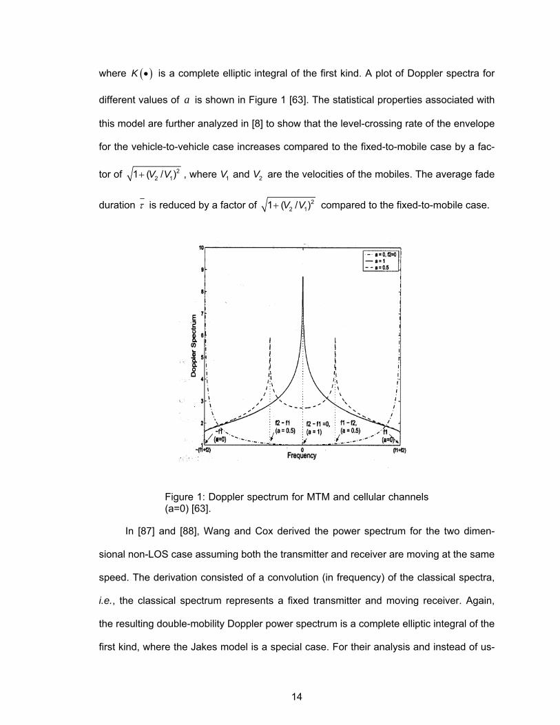
14

where ( )K • is a complete elliptic integral of the first kind. A plot of Doppler spectra for

different values of a is shown in Figure 1 [63]. The statistical properties associated with

this model are further analyzed in [8] to show that the level-crossing rate of the envelope

for the vehicle-to-vehicle case increases compared to the fixed-to-mobile case by a fac-

tor of 22 11 ( / )V V+ , where 1V and 2V are the velocities of the mobiles. The average fade

duration τ is reduced by a factor of 22 11 ( / )V V+ compared to the fixed-to-mobile case.

Figure 1: Doppler spectrum for MTM and cellular channels (a=0) [63].

In [87] and [88], Wang and Cox derived the power spectrum for the two dimen-

sional non-LOS case assuming both the transmitter and receiver are moving at the same

speed. The derivation consisted of a convolution (in frequency) of the classical spectra,

i.e., the classical spectrum represents a fixed transmitter and moving receiver. Again,

the resulting double-mobility Doppler power spectrum is a complete elliptic integral of the

first kind, where the Jakes model is a special case. For their analysis and instead of us-

15

ing a factor multiplying either Doppler frequency, they defined the degree of double mo-

bility as follows:

( )( )

1 2

1 2

min ,, 0 1

max ,V VV V

α α= ≤ ≤ (2.24)

where 1α = is full double mobility and 0α = is single mobility. Although they did not

give a derivation for the case where transmitter velocity is not equal to receiver velocity,

they indicated that as the velocity of the transmitter increases from zero, the vertical as-

ymptotes of the Jakes model move inward. At “full” mobility, when the transmitter and

receiver velocity are equal, the vertical asymptotes merge at the center of the spectrum.

In essence, they arrived to the same spectral shapes as the ones shown in Figure 1, but

they just provided analytical derivations for the extreme cases. They also suggested that

for a fixed maximum Doppler shift, the closer the system is to the full mobility case, it re-

sults in smaller RMS and effective Doppler spread, hence slower fading [87].

The next 2-D study is [63]. Here, Patel introduces the concept of a “double-ring”

mobile-to-mobile scattering environment. This “double-ring” model defines an individual

ring of uniformly spaced scatterers for both the BS and the MS, which causes each

transmitted path to undergo two reflections, one for each ring. For this model, the base-

band received complex envelope is proposed as:

( ) ( ) ( ){ }( )1 21 1

exp 2 cos cosN M

n m nmn m

g t j f f tπ α β θ= =

⎡ ⎤= + +⎣ ⎦∑∑ (2.25)

where index n refers to paths traveling from transmitter to the N scatterers located on the

transmitter ring, and index m refers to the paths traveling from the M scatterers on the

receiver ring to the receiver. The statistical properties of this model match those of the

16

transversal filter model previously described, e.g., its time correlation function is also

given by (2.22).

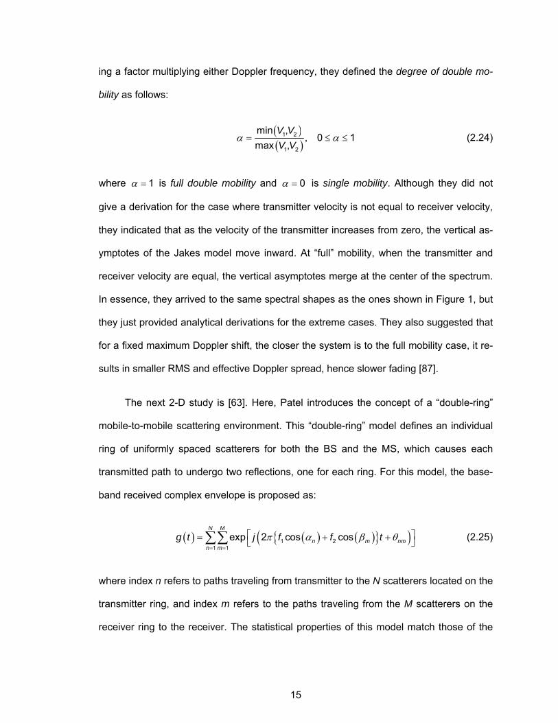
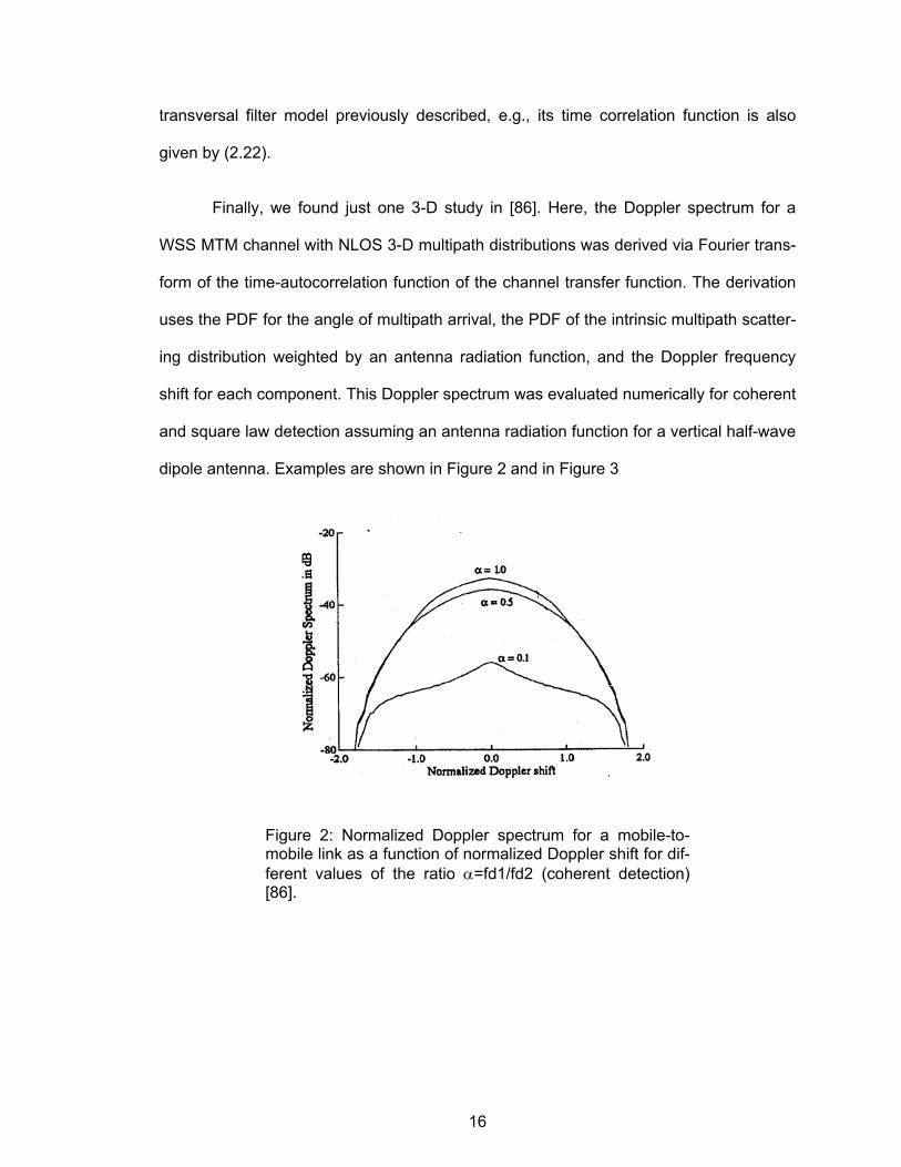
Finally, we found just one 3-D study in [86]. Here, the Doppler spectrum for a

WSS MTM channel with NLOS 3-D multipath distributions was derived via Fourier trans-

form of the time-autocorrelation function of the channel transfer function. The derivation

uses the PDF for the angle of multipath arrival, the PDF of the intrinsic multipath scatter-

ing distribution weighted by an antenna radiation function, and the Doppler frequency

shift for each component. This Doppler spectrum was evaluated numerically for coherent

and square law detection assuming an antenna radiation function for a vertical half-wave

dipole antenna. Examples are shown in Figure 2 and in Figure 3

Figure 2: Normalized Doppler spectrum for a mobile-to-mobile link as a function of normalized Doppler shift for dif-ferent values of the ratio α=fd1/fd2 (coherent detection) [86].

17

Figure 3: Normalized Doppler spectrum for a mobile-to-mobile link as a function of normalized Doppler shift for dif-ferent values of the ratio α=fd1/fd2 (square law detection) [86].

2.1.5 Measured MTM Doppler

One paper [48] contained the flat-fading measurements of vehicle-to-vehicle Dop-

pler shown in Figure 4 for urban and highway environments. In Figure 4, the total power

of each spectrum was normalized to one so that the plots represent the probability den-

sity function of the Doppler frequency fD. It was noted that the Doppler spectrum for the

highway environment was broader than the urban case, as expected since higher rela-

tive velocities occur more frequently in the highway scenario leading to a larger Doppler

spread. Symmetric peaks related to “overtaking situations” are noted for both urban and

highway scenarios.

18

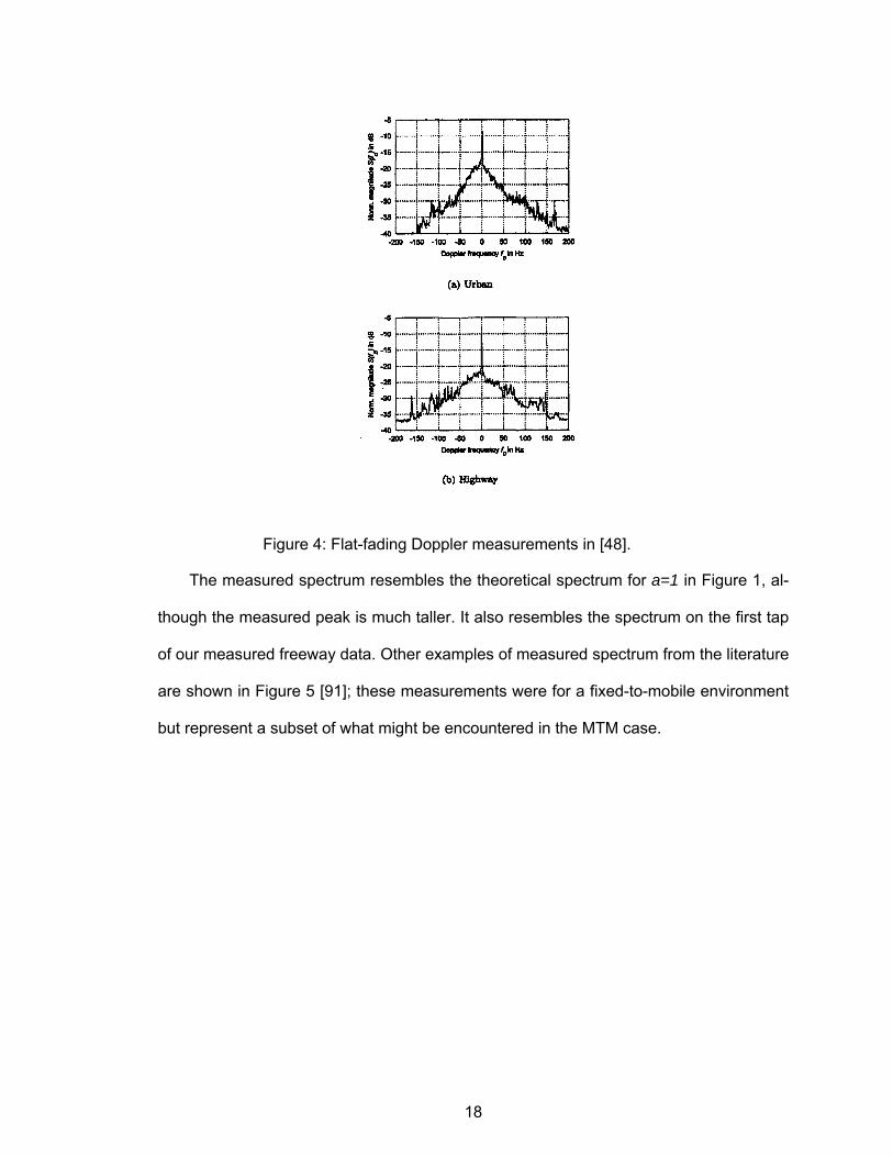
Figure 4: Flat-fading Doppler measurements in [48].

The measured spectrum resembles the theoretical spectrum for a=1 in Figure 1, al-

though the measured peak is much taller. It also resembles the spectrum on the first tap

of our measured freeway data. Other examples of measured spectrum from the literature

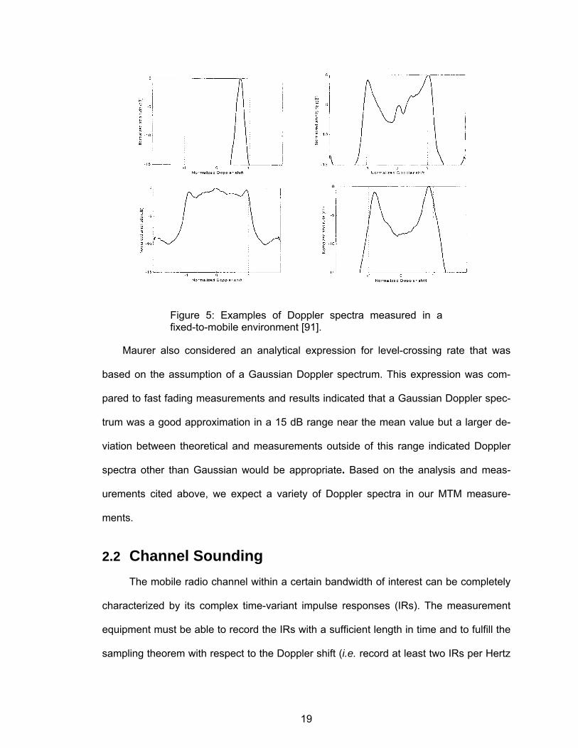
are shown in Figure 5 [91]; these measurements were for a fixed-to-mobile environment

but represent a subset of what might be encountered in the MTM case.

19

Figure 5: Examples of Doppler spectra measured in a fixed-to-mobile environment [91].

Maurer also considered an analytical expression for level-crossing rate that was

based on the assumption of a Gaussian Doppler spectrum. This expression was com-

pared to fast fading measurements and results indicated that a Gaussian Doppler spec-

trum was a good approximation in a 15 dB range near the mean value but a larger de-

viation between theoretical and measurements outside of this range indicated Doppler

spectra other than Gaussian would be appropriate. Based on the analysis and meas-

urements cited above, we expect a variety of Doppler spectra in our MTM measure-

ments.

2.2 Channel Sounding The mobile radio channel within a certain bandwidth of interest can be completely

characterized by its complex time-variant impulse responses (IRs). The measurement

equipment must be able to record the IRs with a sufficient length in time and to fulfill the

sampling theorem with respect to the Doppler shift (i.e. record at least two IRs per Hertz

20

of the maximum Doppler frequency). For system related investigations (e.g., simulations

with stored channel data), a measurement bandwidth equal to the system bandwidth is

sufficient. For the development of (wideband) deterministic or statistical propagation

models, a very large bandwidth for channel measurements is desirable in order to gain

as much detail as possible to enable the understanding of the propagation phenomena

(e.g., identification of scatterer locations) and support the modeling approaches. How-

ever, propagation measurements with large bandwidths produce a huge amount of data.

Narrowband measurements are much simpler to carry out and handle. They are appro-

priate if we require only narrowband information. This is particularly the case for all types

of path-loss modeling [39].

We find in [64] one of the most cited classifications of the available channel sound-

ing techniques where we can fit most of the published works in the last decade. The

techniques are classified as narrowband or wideband and as time- or frequency-domain

approaches.

2.2.1 Narrowband Sounding Techniques

The most common narrowband technique is to excite the channel using an un-

modulated RF carrier (single tone). Large variations are then observed in the amplitude

and phase of the received signal, these variations are a result of the random phase addi-

tions of signals arriving over many scattered paths. Through the years, models like the

Jakes [28] have shown reasonable agreement with single tone measurements of the

fading envelope. One can also perform narrowband Doppler spread measurements by

either recording the channel induced frequency and/or phase modulation of the RF car-

rier or by direct observation of the modulation using a spectrum analyzer.

21

2.2.2 Wideband Sounding Techniques

The evolution of communications systems has dramatically increased the demand

for wideband measurements. There are a number of different approaches to wideband

sounding. In the proposed research, at least two of these approaches will be used to

measure the mobile-to-mobile channel. In this section, we review several techniques,

beginning with the oldest technique of tone-sweeping. We next describe a superior multi-

tone approach, which we will use as a benchmark. To this benchmark, we will compare

several time- and frequency-domain sounding methods, including periodic pulse sound-

ing, pulse compression, chirp sounding, and an OFDM approach. In each case, we will

examine what parameters would be needed to approach the performance of the multi-

tone approach.

2.2.2.1 Tone Stepping

The first wideband measurement attempts relied on sweeping the RF spectrum us-

ing the simple tone technique. In this technique, we step the tones across a band of fre-

quencies to measure the channel frequency transfer function. Using a vector network

analyzer, we can measure the magnitude and phase of the forward transmission gain

21S as if we were exciting a test circuit (in this case the RF channel) with a single sine

wave. This is repeated for a number of equally spaced frequencies within the bandwidth

of interest. Frequency domain channel sounding using network analyzers has two major

drawbacks. First, stepping a synthesizer over a large bandwidth in small steps is time

consuming, and secondly, it is impossible to make mobile measurements due mainly in

part to the strict timing reference requirements, which can be accomplished only through

a wired system. On the other hand, it provides the best multipath resolution and very

small storage requirements. For example, J-S. Jiang [38] used a 500 MHz bandwidth

centered at 5.8 GHz with 401 stepping points and a recording time of six seconds. Such

22

a bandwidth provides a PDP resolution of two nanoseconds, which corresponds to four

wavelengths.

As we can imagine, the tone stepping method is too slow for mobile channels. A

faster alternative would be to perform a real-time frequency domain channel measure-

ment by exciting all frequencies simultaneously and attempting to process and/or record

the reception in real-time. There are two techniques available. The first one uses a

swept frequency (chirp) signal instead of single tone stepping, but the frequency sound-

ing is still sequential. The other one uses a multi-tone signal, and at this time, the

RUSK™ [13] channel sounder is the best representative of this technique, which is also

known as frequency domain correlation processing. For both techniques to work in mo-

bile channels, they require at least real-time recording of baseband complex symbols.

2.2.2.2 The RUSK™ Multitone System

Up until now and to our best knowledge, the state of the art sounding system is the

RUSK™ system. We will briefly describe this system to have a benchmark to compare

the other available techniques. In the RUSK™ system, a signal is sent that includes a

complete set of single tones with 0 1 pf t= Hz of separation. The maximum bandwidth of

the system is 240 MHz, which produces a 3.12 ns resolution. The system has three dif-

ferent repetition periods (IR lengths), 6.4;25.6;102.4 μspt = . The system captures the

signal with an eight bit 640 MHz analog-to-digital (ADC) converter. The system is capa-

ble of recording at a rate of 320 MByte/s using four disk arrays in parallel controlled by a

proprietary interface. All the previous description is about how the system overcomes the

first drawback of the network analyzer system: speed of measurement. To overcome the

second one, which allows for mobile measurements, the system relies on calibrated Ru-

23

bidium frequency generators. We shall describe the characteristics of these frequency

generators in later chapters when we discuss our synchronization method.

There are other alternatives for wideband channel measurements. In the next four

sections we present an overview of the time- and frequency-domain sounding methods

where we show the advantages and disadvantages for each one along with the required

specifications to obtain a similar performance of that of the RUSK™ system previously

described.

2.2.2.3 Periodic Pulse Sounding Method

The CIR is by definition the convolution of the channel response with an ideal pulse

(i.e., infinite magnitude and zero duration). Since there is no such thing as an ideal

pulse, whatever we can measure is only an approximation to the real CIR. On the other

hand, this is a simple channel sounding technique to rapidly determine the power delay

profile of any channel by just detecting the envelope of the received signal and display-

ing it on a high speed oscilloscope. The probing signal is a pulse of width pT with repeti-

tion period RT . The smaller the pulse width is compared to the delay spread of the chan-

nel the better we can resolve the individual multipath components assuming that the pe-

riod exceeds the maximum delay spread, mτ . Of course, the shorter the pulse, the larger

the required null-to-null bandwidth 2 pBW T= for a power spectrum envelope of the

form ( )( )

2sin c p

c p

f f Tf f T

−

−⎡ ⎤⎣ ⎦ . This system is highly sensitive to noise and to interference, and it re-

quires a high peak-to-average power ratio (PAR) to provide adequate detection of weak

echoes [27]. We can detect phase and Doppler shifts using a coherent detector instead

of the envelope detector, but the system loses its simplicity and real time capability.

24

2.2.2.4 Pulse Compression Techniques

To overcome the large dynamic range requirement imposed by the high PAR, we

use pulse compression techniques. The theory of linear systems [62] contains the basis

for all these techniques as follows: if white noise ( )n t is input to a linear system, and if

the system output ( )y t is cross-correlated with a delayed replica of the input ( )n t τ−

then the resulting coefficient is proportional to the IR of the system ( )h t evaluated at the

delay time τ . We will show this below. Let

( ) ( ) ( ) ( )n oE n t n t R Nτ τ δ τ∗⎡ ⎤− = =⎣ ⎦ (2.26)

where ( )nR τ is the autocorrelation function of the noise, and oN is the one-sided noise

power spectral density. The cross-correlation of the system’s output is

0

( ) ( ) ( ) ( ) ( )

( ) ( )

( )n

E y t n t E h n t n t d

h R d

N h

τ λ λ τ λ

λ τ λ λ

τ

∗ ∗⎡ ⎤⎡ ⎤− = − −⎣ ⎦ ⎣ ⎦

= −

=

∫∫ (2.27)

We now need to use an approximation to white noise. We can do it by using maxi-

mum-length pseudo-random binary sequences, which are deterministic signals with

noise-like or pseudo-noise (PN) characteristics. These sequences possess excellent pe-

riodic autocorrelation properties and can be easily generated using linear feedback shift

registers. The general form of one transmitted MLS is

1

0( )cos(2 )

N

n c cn

a g t nT f tπ−

=

−∑ (2.28)

where { } 1

0

Nn n

a −

= is the MLS with { }1, 1na ∈ − + . cT is the “chip” or element period, the pulse

( )cg t nT− is rectangular with width cT , and 2 1pN = − is the length of the sequence.

25

The exponent p is the order of the Galois-field primitive polynomial that generates the

sequence. The first thing we notice is that the MLS is performing a binary phase shift

keying (BPSK) of a carrier with frequency cf ; therefore, we expect a similar spectrum,

( )( )

2sin c c

c c

f f Tf f T

−−

⎡ ⎤⎣ ⎦ and bandwidth 2 cBW T= to the pulse sounding case. Once again, the reso-

lution of the system is given by cT , and T should exceed mτ , but in this case T is also

a function of the dynamic range, 20log( )N , of the signal.

We might consider two main design or performance goals for any channel sounding

system: real time processing or information and real time storage or recording. As an

hypothetical example, let us try to obtain the specifications for a MLS system that

matches the RUSK™ system described previously. We have a 240 MHz bandwidth and

25.6 μsT = . First, we would like the maximum resolution 2 (240 MHz) 8.33 nscT = = ,

then, we want the maximum dynamic range that allows the repetition rate. In this case,

3072cT T = ; therefore, we need to choose between an order 11 (N=2047, T= 17.0 μs, &

66 dB) and an order 12 (N=4095, T= 34.0 μs, & 72 dB) MLS. We choose the latter. Let

us talk about real time recording first. We need at least a 580 MHz ADC. Since we have

chosen the MLS with 72 dB of dynamic range, it would be logical to match it with at least

a 12-bit ADC. This will mean that we need a two-byte word for each quadrature sample

or four bytes per complex sample. The required recording speed is 2.32 GByte/s. As-

suming that there exists a hard disk array that can match the PCI-X bus (latest server

interface bus), we can only achieve 1.064 GByte/s; therefore, there are trade-offs to

solve among dynamic range, repetition rate, and resolution. For this example, we can

first perform some processing before recording. We could combine the complex samples

into a three byte word and decimate by two, which will reduce the speed to 720 MByte/s.

This speed can fit into the PCI-X bus, but it will probably require an array of 16 of the

26

fastest hard drives to match the speed. As we can see, even with the latest technology,

real time recording is hard and expensive.

For real time processing, let us start by looking at the discrete-time correlation op-

eration as follows:

( ) ( )1

0

1 ( )N

xx Ior Qk

R n r n a kN

−

=

= ∑ (2.29)

where ( )r n is the received baseband quadrature signal, and ( )a k is the stored MLS.

For each complex baseband sample, we need 2N operations, which for our example

translate into 4.42 TFLOPS, way out of the reach of even the most powerful DSP. There-

fore, in cases like our example, it makes more sense to bias the design efforts towards

recording capability for off-line or post-processing.

In case of continuous-time processing, there are two main techniques to perform the

correlation process. The first one is the convolution matched-filter technique where a

filter is designed to match the sounding waveform. This means that the filter must match

the specific MLS by implementing a transversal or finite impulse response (FIR) filter

with a MLS used as the tap weights. CMOS switched-capacitor circuits (SC), charged-

coupled devices (CCD), and surface-acoustic wave (SAW) technologies are all viable

solutions for this task. SAW devices are most suitable for high-frequency operation while

the others are preferable in digital CMOS compatible solutions [61]. Such a system will

operate in real time, but the recording requirements do not change. Also, the perform-

ance of practical SAW devices is limited by their own deficiencies. Specifically, long se-

quences are difficult to obtain, and the generation of spurious acoustic signals that along

with other inherent imperfections cause time sidelobes to appear at the output of the fil-

ter. These sidelobes reduce the sensitivity to weak echoes.

27

The second technique is the swept time-delay cross-correlation (STDCC)

method. This method focuses on real time processing and data reduction to allow re-

cording. For real time processing, a local MLS is generated and mixed with the incoming

signal usually at IF. This requires a stable synchronization, which once again is usually

achieved by means of a Rubidium generator. In a sense, we have to duplicate the whole

transmitter generator, but there is a big problem. It is not just a matter of running the two

generators in parallel; we cannot achieve the correlation function this way. What we will

need to do is to start the local MLS at least every delay lag chosen as the system resolu-

tion, which is of course clearly unrealistic since it would require a huge bank of genera-

tors. There is an alternative that not only allows real-time correlation, but it also reduces

the recording requirements. This idea dates back to 1972 [21] and relies in a time-

scaling of the IR estimate [81]. To explain the time-scaling, we start by looking at an

ideal discrete-time signal illustrated in Figure 6. By ideal, we mean as if we were able to

process the sequences digitally with perfect synchronization. Here we show the first

elements of the transmitted sequence with elementary or chip period cT , the sequence

generated at the receiver with a chip period crT , and the period psT , where we have a

maximum value for the correlation between the two sequences. As we can see, the pe-

riod of the receiver sequence is slightly longer than the transmitted period. We can easily

accomplish this by offsetting the reference generators by a small amount. There will be

an instant when the first elements of two sequences align at 0t = . From this instant,

they will start separating or offsetting at a rate ( )cr cN T TΔ = − for each sequence repeti-

28

cr cT T>cT

0t =

t = Δ

2t = Δ

3t = Δ

ps cT kT=

Figure 6: First elements of transmitted and locally gener-ated sequences shown for three transmitted sequence repetition cycles.

tion cycle ,rep TX cT NT= . If we consider the trailing edge of the receiver’s sequence first

element as the correlation instant (i.e., the sampling instant), we can fit cT Δ correlation

instants before the sequences have to align again. Therefore, both sequences will sus-

tain correlation for a period ps cT kT= where ( )c cr ck T T T= − is the slide factor. We have

indeed extended or time-dilated the correlation period to , ,rep STDCC rep TXT kT= , and the re-

sulting output will resemble a pulsed signal with pulse width psT , repetition rate ,rep STDCCT ,

and amplitude N . For each reflected path, the receiver’s sequence will correlate in the

same manner; therefore, the delay spread measurement obtained will also be time-

dilated. To obtain the original or real delay spread, we have to scale the measurement

dividing by k . As we mentioned before, the correlation operation is usually performed at

IF in the STDCC systems using a mixer to multiply the signals followed by an integrator.

29

The equivalent baseband operations is as follows: we start with just one transmitter se-

quence and one receiver sequence aligned at 0t =

1

01

0

( ) ( )

( ) ( )

N

TX n cn

N

RX k crk

s t a g t nT

s t a g t kT

−

=

−

=

= −

′= −

∑

∑ (2.30)

where g′ has width crT . During the correlation period, the receiver sequence advances

at Δ intervals

1

0( , ) ( );

N

RX n crn

s t m a g t nT m−

=

= − − Δ∑ (2.31)

therefore, the output of the correlator is

0

1 1

0 0 0

( ) ( ) ( , )

( ) ( ) ,

c

c

NT

TX RX

NTN N

n k c crn k

c m s t s t m dt

a a g t nT g t kT m dt− −

= =

=

′= − − − Δ

∫

∑∑ ∫ (2.32)

which is reference to the transmitter chip period cT . The maximum value of the correla-

tion will occur when the sequences’ overlapping is a maximum as we can see in the top

graph of Figure 6. Since the areas will start overlapping from the left for the next align-

ment instant, the resulting shape of ( )c m is a triangular pulse similar to the convolution

of two rectangular pulses as we describe in Figure 7.

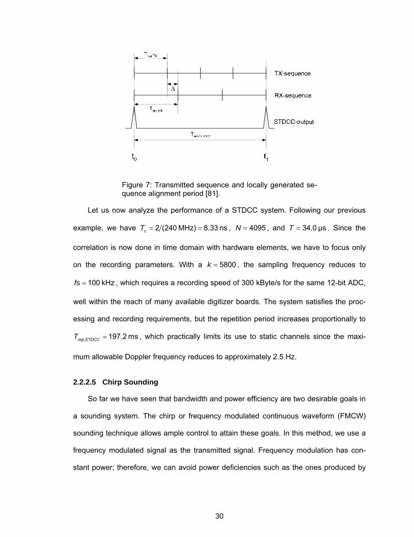
30

Δ

Figure 7: Transmitted sequence and locally generated se-quence alignment period [81].

Let us now analyze the performance of a STDCC system. Following our previous

example, we have 2 (240 MHz) 8.33 nscT = = , 4095N = , and 34.0 μsT = . Since the

correlation is now done in time domain with hardware elements, we have to focus only

on the recording parameters. With a 5800k = , the sampling frequency reduces to

100 kHzfs = , which requires a recording speed of 300 kByte/s for the same 12-bit ADC,

well within the reach of many available digitizer boards. The system satisfies the proc-

essing and recording requirements, but the repetition period increases proportionally to

, 197.2 msrep STDCCT = , which practically limits its use to static channels since the maxi-

mum allowable Doppler frequency reduces to approximately 2.5 Hz.

2.2.2.5 Chirp Sounding

So far we have seen that bandwidth and power efficiency are two desirable goals in

a sounding system. The chirp or frequency modulated continuous waveform (FMCW)

sounding technique allows ample control to attain these goals. In this method, we use a

frequency modulated signal as the transmitted signal. Frequency modulation has con-

stant power; therefore, we can avoid power deficiencies such as the ones produced by

31

large PAR. The transmitted baseband signal is usually a linear frequency modulated

continuous signal of the form

( )2( ) cos 2Hs t A t tω β= + (2.33)

where A is the signal amplitude, 2H Hfω π= is the initial frequency, and tβ ω= ∂ ∂ is the

rate of frequency variation. This signal has an almost constant spectrum over the swept

bandwidth in contrast to the square sinc shape of the STDCC. Its multipath resolution is

1 BW , and its unambiguous Doppler coverage is 1 2T± .

At the receiver, the chirp signal is compressed by either a matched filter in a similar

manner to the sliding correlator, e.g., via SAW filters, but with the same limitations and

advantages as before. Another way to measure the individual time delays of the multi-

path arrivals is to combine the received signal with the transmitted signal using a mixer.

This homodyne signal contains frequencies, called beat frequencies, which are propor-

tional to the time delays of the multipath arrivals. Since this method requires strictly iden-

tical chirp-signal characteristics and simultaneous synchronization in both transmitter

and receiver, homodyne reception is highly desirable, but it limits the use of the system

to static measurements. Once again, using highly stable Rubidium reference generators,

we can achieve heterodyne reception.

The output of this detection method is compressed in frequency but not compressed

in time. The required bandwidth at the output of the detector is determined by the prod-

uct of the sweep rate and the maximum expected time delay of the farthest echo. This

results in an important reduction in bandwidth without a significant reduction in the effec-

tive repetition rate of the sounder. The disadvantage of the chirp sounder is that the

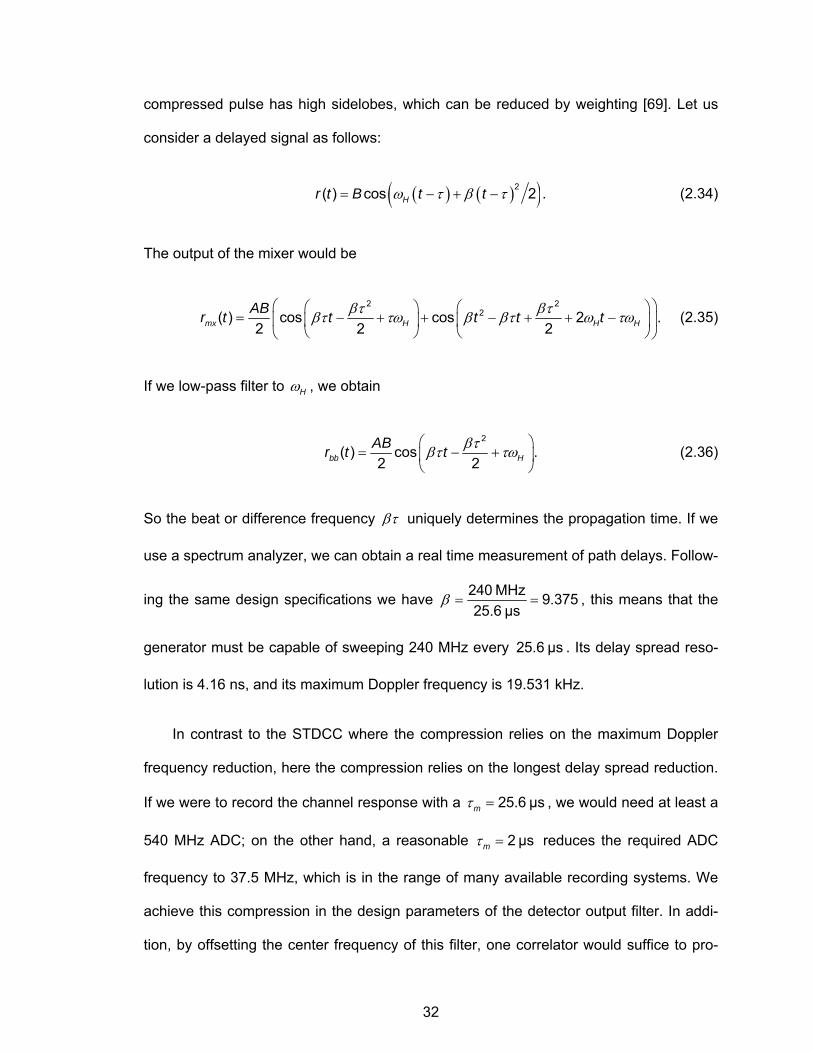
32

compressed pulse has high sidelobes, which can be reduced by weighting [69]. Let us

consider a delayed signal as follows:

( ) ( )( )2( ) cos 2 .Hr t B t tω τ β τ= − + − (2.34)

The output of the mixer would be

2 2

2( ) cos cos 2 .2 2 2mx H H H

ABr t t t t tβτ βτβτ τω β βτ ω τω⎛ ⎞⎛ ⎞ ⎛ ⎞

= − + + − + + −⎜ ⎟⎜ ⎟ ⎜ ⎟⎝ ⎠ ⎝ ⎠⎝ ⎠

(2.35)

If we low-pass filter to Hω , we obtain

2

( ) cos .2 2bb H

ABr t t βτβτ τω⎛ ⎞

= − +⎜ ⎟⎝ ⎠

(2.36)

So the beat or difference frequency βτ uniquely determines the propagation time. If we

use a spectrum analyzer, we can obtain a real time measurement of path delays. Follow-

ing the same design specifications we have 240 MHz 9.37525.6 μs

β = = , this means that the

generator must be capable of sweeping 240 MHz every 25.6 μs . Its delay spread reso-

lution is 4.16 ns, and its maximum Doppler frequency is 19.531 kHz.

In contrast to the STDCC where the compression relies on the maximum Doppler

frequency reduction, here the compression relies on the longest delay spread reduction.

If we were to record the channel response with a 25.6 μsmτ = , we would need at least a

540 MHz ADC; on the other hand, a reasonable 2 μsmτ = reduces the required ADC

frequency to 37.5 MHz, which is in the range of many available recording systems. We

achieve this compression in the design parameters of the detector output filter. In addi-

tion, by offsetting the center frequency of this filter, one correlator would suffice to pro-

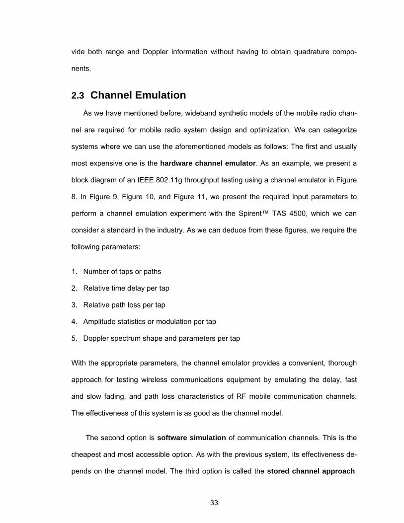
33

vide both range and Doppler information without having to obtain quadrature compo-

nents.

2.3 Channel Emulation As we have mentioned before, wideband synthetic models of the mobile radio chan-

nel are required for mobile radio system design and optimization. We can categorize

systems where we can use the aforementioned models as follows: The first and usually

most expensive one is the hardware channel emulator. As an example, we present a

block diagram of an IEEE 802.11g throughput testing using a channel emulator in Figure

8. In Figure 9, Figure 10, and Figure 11, we present the required input parameters to

perform a channel emulation experiment with the Spirent™ TAS 4500, which we can

consider a standard in the industry. As we can deduce from these figures, we require the

following parameters:

1. Number of taps or paths

2. Relative time delay per tap

3. Relative path loss per tap

4. Amplitude statistics or modulation per tap

5. Doppler spectrum shape and parameters per tap

With the appropriate parameters, the channel emulator provides a convenient, thorough

approach for testing wireless communications equipment by emulating the delay, fast

and slow fading, and path loss characteristics of RF mobile communication channels.

The effectiveness of this system is as good as the channel model.

The second option is software simulation of communication channels. This is the

cheapest and most accessible option. As with the previous system, its effectiveness de-

pends on the channel model. The third option is called the stored channel approach.

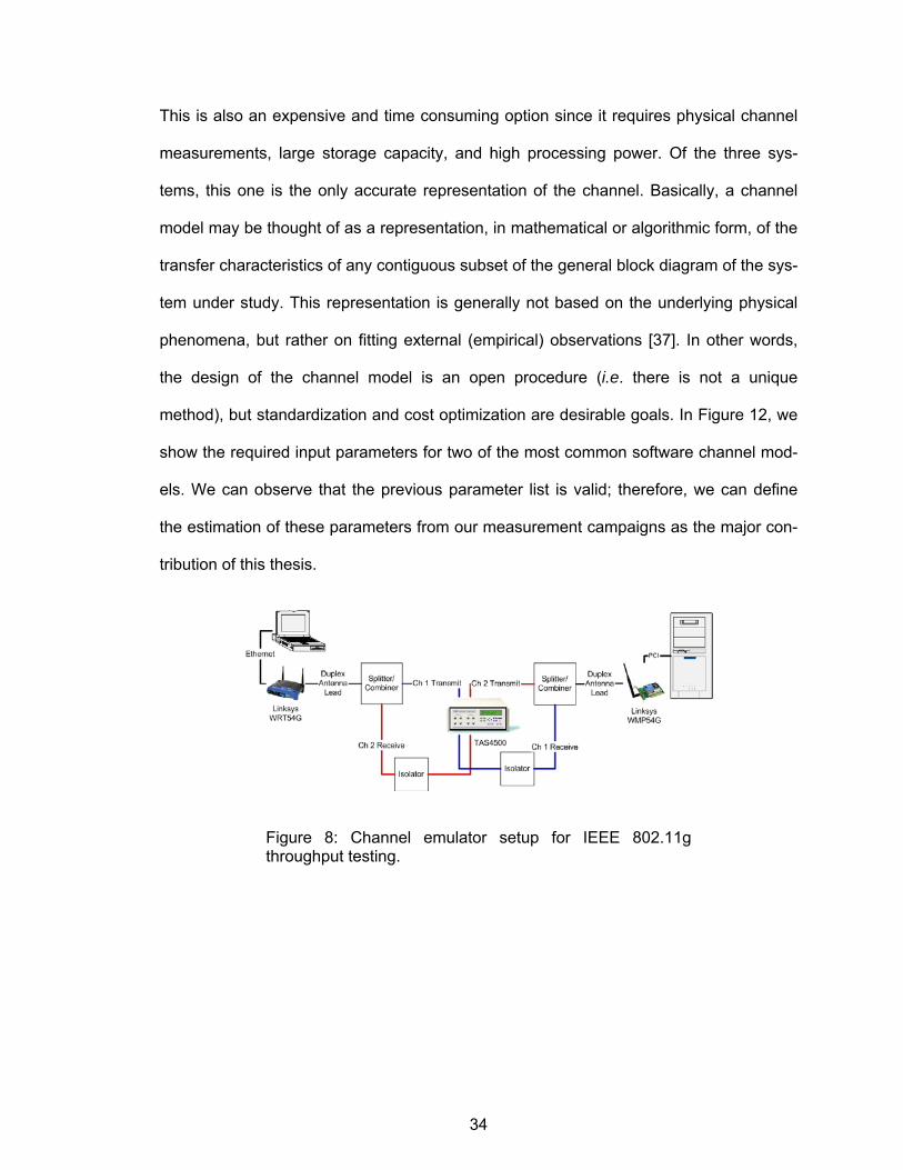
34

This is also an expensive and time consuming option since it requires physical channel

measurements, large storage capacity, and high processing power. Of the three sys-

tems, this one is the only accurate representation of the channel. Basically, a channel

model may be thought of as a representation, in mathematical or algorithmic form, of the

transfer characteristics of any contiguous subset of the general block diagram of the sys-

tem under study. This representation is generally not based on the underlying physical

phenomena, but rather on fitting external (empirical) observations [37]. In other words,

the design of the channel model is an open procedure (i.e. there is not a unique

method), but standardization and cost optimization are desirable goals. In Figure 12, we

show the required input parameters for two of the most common software channel mod-

els. We can observe that the previous parameter list is valid; therefore, we can define

the estimation of these parameters from our measurement campaigns as the major con-

tribution of this thesis.

Figure 8: Channel emulator setup for IEEE 802.11g throughput testing.

35

(a) (b)

Figure 9: Spirent TAS 4500 hardware channel emulator parameters setup: (a) number of taps and (b) delay per tap.

(a) (b)

Figure 10: Spirent TAS 4500 hardware channel emulator parameters setup: (a) Doppler parameters per tap and (b) power per tap.

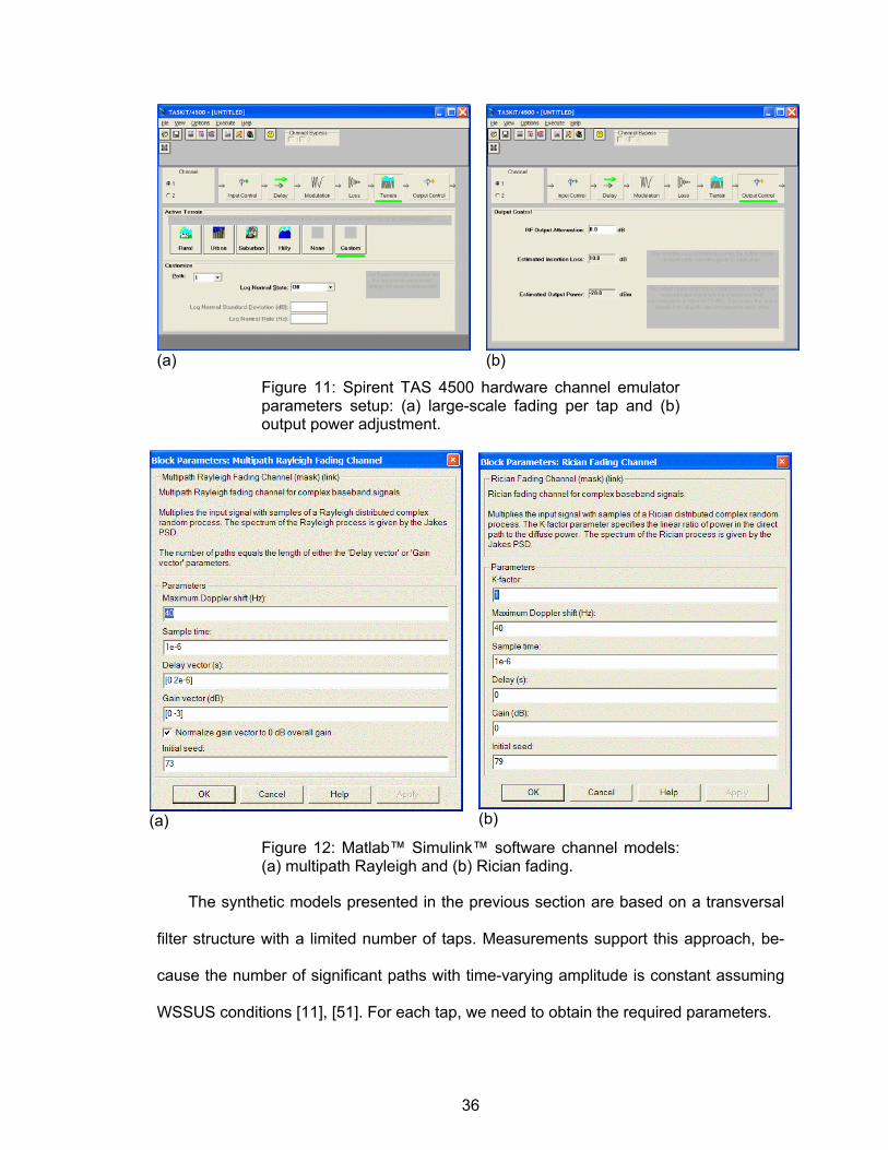
36

(a) (b)

Figure 11: Spirent TAS 4500 hardware channel emulator parameters setup: (a) large-scale fading per tap and (b) output power adjustment.

(a) (b)

Figure 12: Matlab™ Simulink™ software channel models: (a) multipath Rayleigh and (b) Rician fading.

The synthetic models presented in the previous section are based on a transversal

filter structure with a limited number of taps. Measurements support this approach, be-

cause the number of significant paths with time-varying amplitude is constant assuming

WSSUS conditions [11], [51]. For each tap, we need to obtain the required parameters.

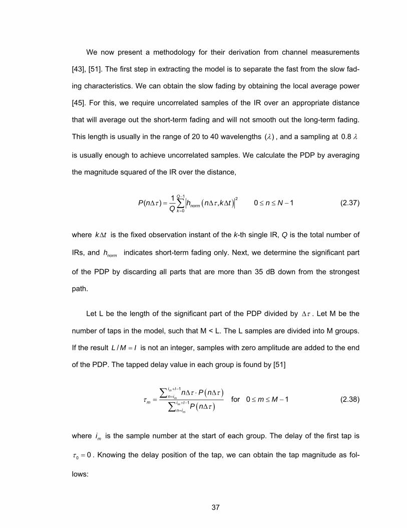
37

We now present a methodology for their derivation from channel measurements

[43], [51]. The first step in extracting the model is to separate the fast from the slow fad-

ing characteristics. We can obtain the slow fading by obtaining the local average power

[45]. For this, we require uncorrelated samples of the IR over an appropriate distance

that will average out the short-term fading and will not smooth out the long-term fading.

This length is usually in the range of 20 to 40 wavelengths λ( ) , and a sampling at λ0.8

is usually enough to achieve uncorrelated samples. We calculate the PDP by averaging

the magnitude squared of the IR over the distance,

( )τ τ−

=

Δ = Δ Δ ≤ ≤ −∑1 2

0

1( ) , 0 1Q

normk

P n h n k t n NQ

(2.37)

where k tΔ is the fixed observation instant of the k-th single IR, Q is the total number of

IRs, and normh indicates short-term fading only. Next, we determine the significant part

of the PDP by discarding all parts that are more than 35 dB down from the strongest

path.

Let L be the length of the significant part of the PDP divided by τΔ . Let M be the

number of taps in the model, such that M < L. The L samples are divided into M groups.

If the result /L M I= is not an integer, samples with zero amplitude are added to the end

of the PDP. The tapped delay value in each group is found by [51]

( )

( )τ τ

ττ

+ −

=+ −

=

Δ ⋅ Δ= ≤ ≤ −

Δ

∑∑

1

1 for 0 1m

m

m

m

i I

n im i I

n i

n P nm M

P n (2.38)

where mi is the sample number at the start of each group. The delay of the first tap is

0 0τ = . Knowing the delay position of the tap, we can obtain the tap magnitude as fol-

lows:

38

( ) ( )τ τ+ −

=

Δ = Δ Δ∑11, , .

m

m

i I

m mn i

P k t P n k tI

(2.39)

We determine the Rice factor for each tap using the moment-method [1], [29] as follows:

( )

( )

τ

σ

σ

=

=

= Δ =

=

= −

= −

= −

=

∑

∑

K2

1

2

1

2 2 2

22

2

2

, , 1, ,

1

1

.

k m m

Q

a kk

Q

v k ak

a v

a

Rice

G h k t k Q

G GQ

G G GQ

V G G

G V

VK

(2.40)

Finally, we use the Welch algorithm to estimate the Doppler spectrum per tap.

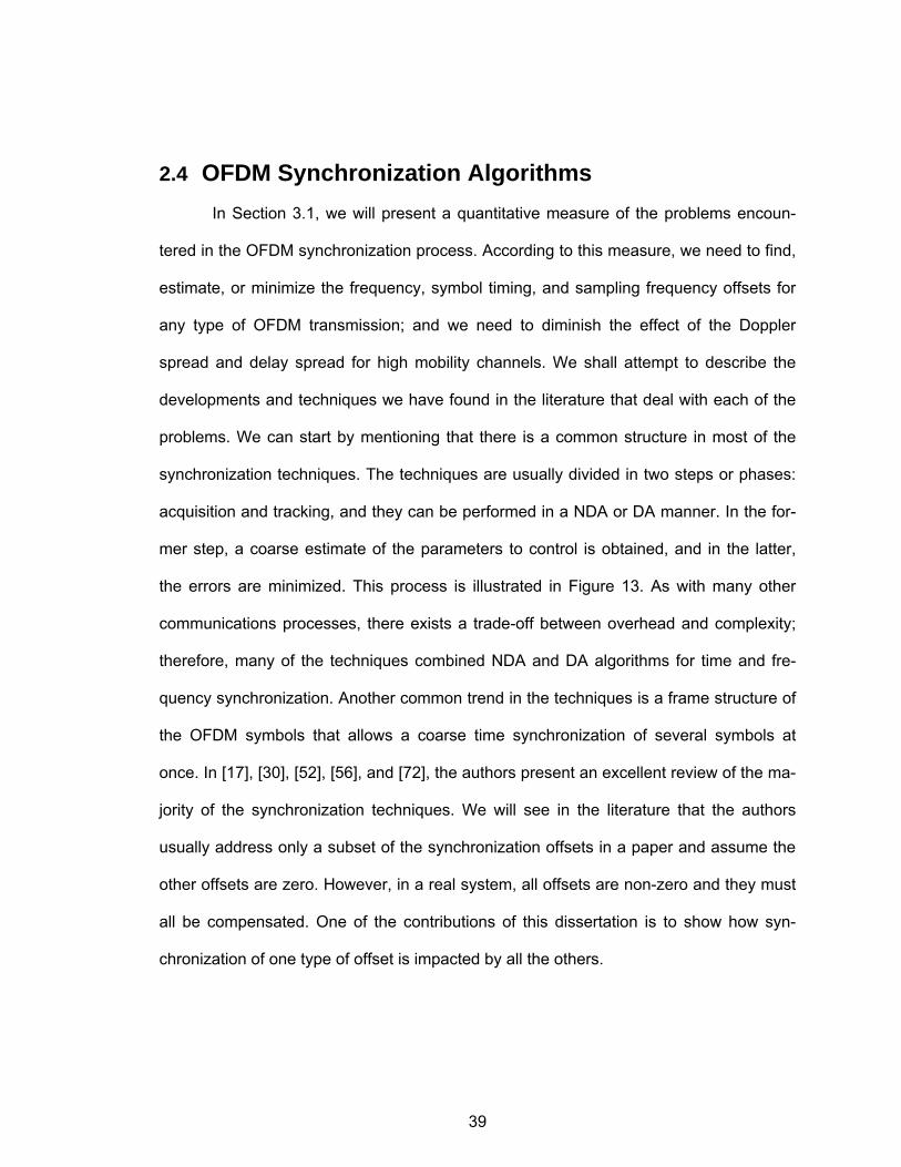
39

2.4 OFDM Synchronization Algorithms In Section 3.1, we will present a quantitative measure of the problems encoun-

tered in the OFDM synchronization process. According to this measure, we need to find,

estimate, or minimize the frequency, symbol timing, and sampling frequency offsets for

any type of OFDM transmission; and we need to diminish the effect of the Doppler

spread and delay spread for high mobility channels. We shall attempt to describe the

developments and techniques we have found in the literature that deal with each of the

problems. We can start by mentioning that there is a common structure in most of the

synchronization techniques. The techniques are usually divided in two steps or phases:

acquisition and tracking, and they can be performed in a NDA or DA manner. In the for-

mer step, a coarse estimate of the parameters to control is obtained, and in the latter,

the errors are minimized. This process is illustrated in Figure 13. As with many other

communications processes, there exists a trade-off between overhead and complexity;

therefore, many of the techniques combined NDA and DA algorithms for time and fre-

quency synchronization. Another common trend in the techniques is a frame structure of

the OFDM symbols that allows a coarse time synchronization of several symbols at

once. In [17], [30], [52], [56], and [72], the authors present an excellent review of the ma-

jority of the synchronization techniques. We will see in the literature that the authors

usually address only a subset of the synchronization offsets in a paper and assume the

other offsets are zero. However, in a real system, all offsets are non-zero and they must

all be compensated. One of the contributions of this dissertation is to show how syn-

chronization of one type of offset is impacted by all the others.

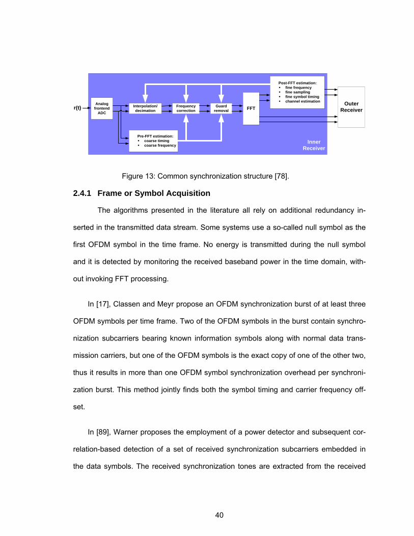
40

Frequencycorrection

Guardremoval FFT

Post-FFT estimation:fine frequencyfine samplingfine symbol timingchannel estimation Outer

Receiver

Pre-FFT estimation:coarse timingcoarse frequency

Analogfrontend

ADC

Interpolation/decimationr(t)

InnerReceiver

Figure 13: Common synchronization structure [78].

2.4.1 Frame or Symbol Acquisition

The algorithms presented in the literature all rely on additional redundancy in-

serted in the transmitted data stream. Some systems use a so-called null symbol as the

first OFDM symbol in the time frame. No energy is transmitted during the null symbol

and it is detected by monitoring the received baseband power in the time domain, with-

out invoking FFT processing.

In [17], Classen and Meyr propose an OFDM synchronization burst of at least three

OFDM symbols per time frame. Two of the OFDM symbols in the burst contain synchro-

nization subcarriers bearing known information symbols along with normal data trans-

mission carriers, but one of the OFDM symbols is the exact copy of one of the other two,

thus it results in more than one OFDM symbol synchronization overhead per synchroni-

zation burst. This method jointly finds both the symbol timing and carrier frequency off-

set.

In [89], Warner proposes the employment of a power detector and subsequent cor-

relation-based detection of a set of received synchronization subcarriers embedded in

the data symbols. The received synchronization tones are extracted from the received

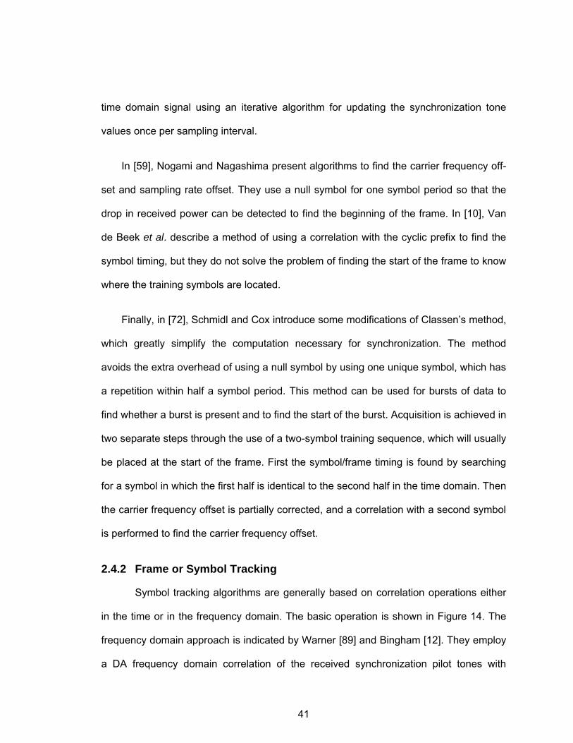
41

time domain signal using an iterative algorithm for updating the synchronization tone

values once per sampling interval.

In [59], Nogami and Nagashima present algorithms to find the carrier frequency off-

set and sampling rate offset. They use a null symbol for one symbol period so that the

drop in received power can be detected to find the beginning of the frame. In [10], Van

de Beek et al. describe a method of using a correlation with the cyclic prefix to find the

symbol timing, but they do not solve the problem of finding the start of the frame to know

where the training symbols are located.

Finally, in [72], Schmidl and Cox introduce some modifications of Classen’s method,

which greatly simplify the computation necessary for synchronization. The method

avoids the extra overhead of using a null symbol by using one unique symbol, which has

a repetition within half a symbol period. This method can be used for bursts of data to

find whether a burst is present and to find the start of the burst. Acquisition is achieved in

two separate steps through the use of a two-symbol training sequence, which will usually

be placed at the start of the frame. First the symbol/frame timing is found by searching

for a symbol in which the first half is identical to the second half in the time domain. Then

the carrier frequency offset is partially corrected, and a correlation with a second symbol

is performed to find the carrier frequency offset.

2.4.2 Frame or Symbol Tracking

Symbol tracking algorithms are generally based on correlation operations either

in the time or in the frequency domain. The basic operation is shown in Figure 14. The

frequency domain approach is indicated by Warner [89] and Bingham [12]. They employ

a DA frequency domain correlation of the received synchronization pilot tones with

42

known synchronization sequences. A time domain NDA correlation can be performed as

de Couasnon [18] and Sandell’s [70] groups suggest. The former utilizes the redundancy

of the cyclic prefix by integrating over the magnitude of the difference between the data

and the cyclic extension samples. The latter proposes exploiting the autocorrelation

properties of the received time domain samples imposed by the cyclic extension for fine

time domain tracking.

Tdelay Conjugation

Estimatephase ofmaximum

Findmaximumcorrelation

dt∫OFDMsignal

Frequencyoffset

Timing

Figure 14: Basic correlation process.

2.4.3 Frequency Offset Acquisition

The frequency offset acquisition algorithm has to provide an initial frequency error

estimate, which is sufficiently accurate for the subsequent frequency-tracking algorithm

to operate reliably. Generally, the initial estimate must be accurate to half a subcarrier

spacing. For the acquisition process, most of the techniques use DA algorithms.

In [71], Sari proposes the use of a pilot tone embedded into the data symbol, sur-

rounded by zero-valued virtual subcarriers, so that the receiver can locate the frequency-

shifted pilot easily.

In [54], Moose gives the ML estimator for the carrier frequency offset that is calcu-

lated in the frequency domain after taking the FFT. He assumes that the symbol timing is

known, so he just has to find the carrier frequency offset. The limit of the acquisition

43

range for the carrier frequency offset is 1 2± the subcarrier spacing. He also describes

how to increase this range by using shorter training symbols to find the carrier frequency

offset. For example, shortening the training symbols by a factor of two would double the

range of carrier frequency acquisition. This approach will work to a point, but the esti-

mates get worse as the symbols get shorter because there are fewer samples over

which to average, and the training symbols need to be kept longer than the guard inter-

val so that the channel impulse response does not cause distortion when estimating the

frequency offset.

In [17], Classen and Meyr propose to use binary PN or so-called constant ampli-

tude, zero autocorrelation (CAZAC) training sequences carried by synchronization sub-

carriers, which are also employed for the frequency tracking. The frequency acquisition,

however, is performed by a search for the training sequence in the frequency domain.

This is achieved by means of frequency domain correlation of the received symbol with

the training sequence. The method is very computationally complex because it uses a

trial and error method where the carrier frequency is incremented in small steps over the

entire acquisition range until the correct carrier frequency is found. It is impractical to do

the exhaustive search and go through a large amount of computation at each possible

carrier frequency offset.

Lastly in [72], Schmidl and Cox employ different OFDM blocks. The first one has two

identical halves and serves to measure the frequency offset with an ambiguity of multi-

ples of the sub-carrier spacing. The second block contains a pseudo-noise sequence

and serves to resolve the frequency ambiguity.

44

2.4.4 Frequency Offset Tracking

The frequency offset tracking method generally relies on an already established

coarse frequency estimation having a frequency error of less than half a subcarrier spac-

ing. In [54], Moose suggests the use of the phase difference between subcarriers of re-

peated OFDM symbols in order to estimate frequency deviations of up to one-half of the

subcarrier spacing.

In [17], Classen and Meyr employ frequency domain synchronization subcarriers

embedded into the data symbols, for which the phase shift between consecutive OFDM

symbols can be measured. Also in [23] and [70], and Daffara and Sandell respectively,

use the phase of the received signal’s autocorrelation function, which represents a

phase shift between the received data samples and their repeated copies in the cyclic

extension of the OFDM symbols.

2.4.5 Sampling Frequency Offset Acquisition

Simoens et al [73] propose a joint ML algorithm to estimate the frequency offset and

the sampling frequency offset. Under certain assumptions a linearization can be applied,

leading to an analytical expression of the estimator. Sliskovic [76], [77] estimates the

sampling frequency offset using the repetition of data symbols and comparison of the

phases between successive repeated symbols on all subcarriers. The phase difference

between successive symbols has two mains causes: either frequency offset or sampling

frequency offset. Sliskovic assumes that there is no frequency offset.

One major conclusion from the OFDM synchronization literature survey is that ML

estimation of the OFDM synchronization offsets provides high accuracy [19], [20], [24].

Several authors have considered ML for one or two offsets [10], [73], [76], [77]. We need

45

to estimate all of them; however, joint estimation of all them has too much complexity. In

the next chapter, we discuss our adopted approach for OFDM synchronization.

46

CHAPTER 3

OFDM SYNCHRONIZATION

OFDM systems have become widely popular since the beginning of the 1990s. We

can find them as the preferred physical layer (PHY) in many transmission standards

such as: DAB, IBOC, DVB, DSRC, IEEE 802.11a, IEEE 802.11g, IEEE 802.11p, IEEE

802.16. OFDM importance will continue to grow along with the wideband requirements

of future communication systems; therefore, in this chapter, we present an analysis of

one of its weaknesses: synchronization offsets. In the first part of the chapter, we offer a

detailed analysis of the degradation produced by these offsets. We will extend the

analysis to a static channel. In the second part, we propose a technique to detect and

compensate for them that will be useful in a situation where we need to develop a trans-

ceiver test bed with fixed parameter components. By fixed parameters, we mean for ex-

ample an ADC board with a fixed clock. This proposed technique is by no means in-

tended for a real-time communication system. Its main purpose is to provide a tool that

will help in the development or calibration of a prototype system.

3.1 OFDM Synchronization Offsets Previous works in the literature have focused only on subsets of these offsets, and

most of these works are referenced to [65]. In particular, we find in [80] one of the few

that includes an analysis of all the offsets; however, they are treated singly. In these few,

we also have [50], but in this work, Mody made approximations to reduce the expression

complexity. We derived most of this work from the experiences and problems encoun-

tered in our experimental test-bed. In our test-bed, we had only one clock for all the

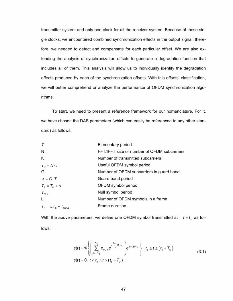
47

transmitter system and only one clock for all the receiver system. Because of these sin-

gle clocks, we encountered combined synchronization effects in the output signal; there-

fore, we needed to detect and compensate for each particular offset. We are also ex-

tending the analysis of synchronization offsets to generate a degradation function that

includes all of them. This analysis will allow us to individually identify the degradation

effects produced by each of the synchronization offsets. With this offsets’ classification,

we will better comprehend or analyze the performance of OFDM synchronization algo-

rithms.

To start, we need to present a reference framework for our nomenclature. For it,

we have chosen the DAB parameters (which can easily be referenced to any other stan-

dard) as follows:

T Elementary period N FFT/IFFT size or number of OFDM subcarriers K Number of transmitted subcarriers

= ⋅UT N T Useful OFDM symbol period G Number of OFDM subcarriers in guard band

Δ = ⋅G T Guard band period

= + ΔS UT T OFDM symbol period

NULLT Null symbol period L Number of OFDM symbols in a frame

= +F S NULLT LT T Frame duration.

With the above parameters, we define one OFDM symbol transmitted at st t= as fol-

lows:

( ) ( ) ( )

( )

ππ

−−

=−

⎧ ⎫⎛ ⎞⎪ ⎪⎜ ⎟= ℜ ≤ ≤ +⎨ ⎬⎜ ⎟⎪ ⎪⎝ ⎠⎩ ⎭= < ∧ > +

∑ U

K 22T

, ,K

2

( ) c ,

( ) 0,

sc s

kj t tj f t t

m l k s s Uk

s s U

s t e e t t t T

s t t t t t T

(3.1)

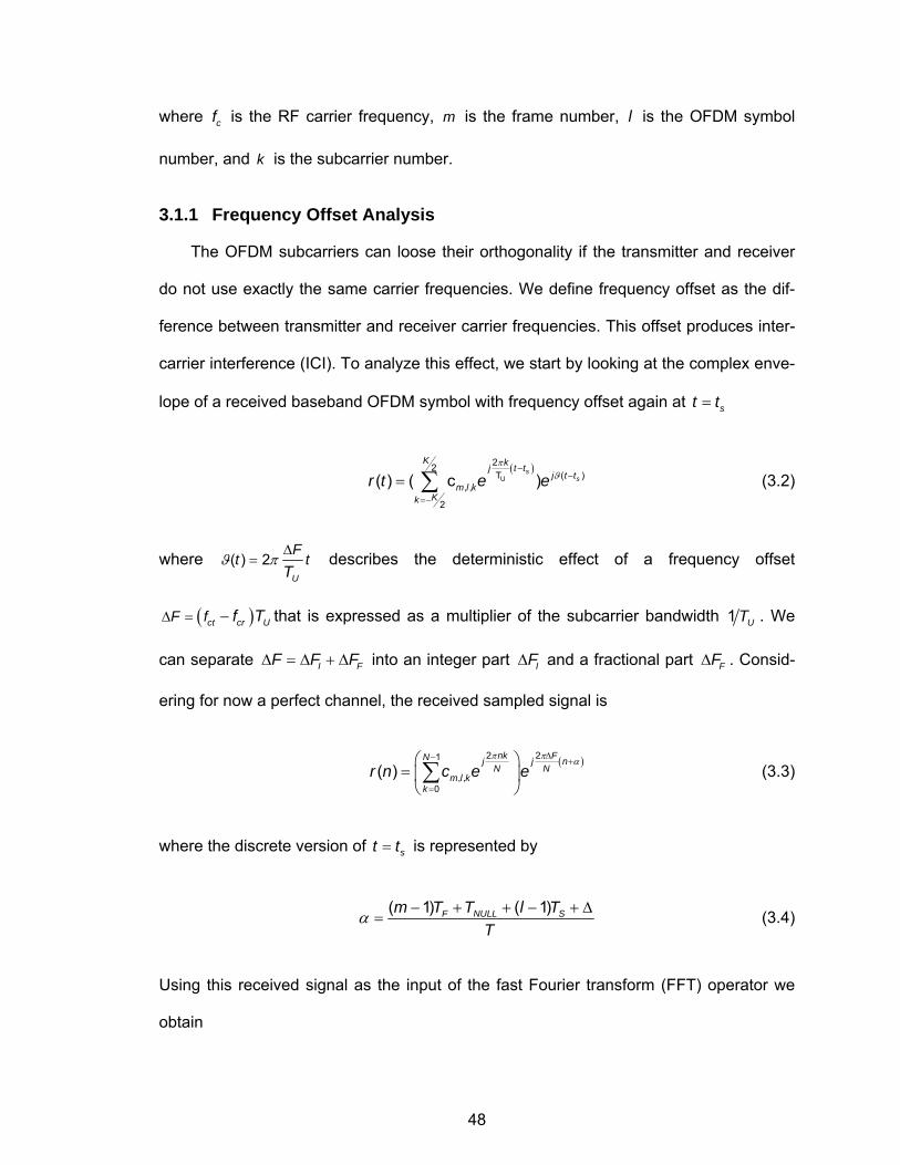
48

where cf is the RF carrier frequency, m is the frame number, l is the OFDM symbol

number, and k is the subcarrier number.

3.1.1 Frequency Offset Analysis

The OFDM subcarriers can loose their orthogonality if the transmitter and receiver

do not use exactly the same carrier frequencies. We define frequency offset as the dif-

ference between transmitter and receiver carrier frequencies. This offset produces inter-

carrier interference (ICI). To analyze this effect, we start by looking at the complex enve-

lope of a received baseband OFDM symbol with frequency offset again at st t=

( )π

ϑ−

−

=−

= ∑ U

22T ( )

, ,

2

( ) ( c )s

s

K kj t tj t t

m l kKk

r t e e (3.2)

where ϑ πΔ

=( ) 2U

Ft t

T describes the deterministic effect of a frequency offset

( )Δ = −ct cr UF f f T that is expressed as a multiplier of the subcarrier bandwidth 1 UT . We

can separate Δ = Δ + ΔI FF F F into an integer part Δ IF and a fractional part Δ FF . Consid-

ering for now a perfect channel, the received sampled signal is

( )π π αΔ− +

=

⎛ ⎞= ⎜ ⎟⎝ ⎠∑

2 21

, ,0

( )nk FN j j n

N Nm l k

kr n c e e (3.3)

where the discrete version of st t= is represented by

α − + + − + Δ=

( 1) ( 1)F NULL Sm T T l TT

(3.4)

Using this received signal as the input of the fast Fourier transform (FFT) operator we

obtain

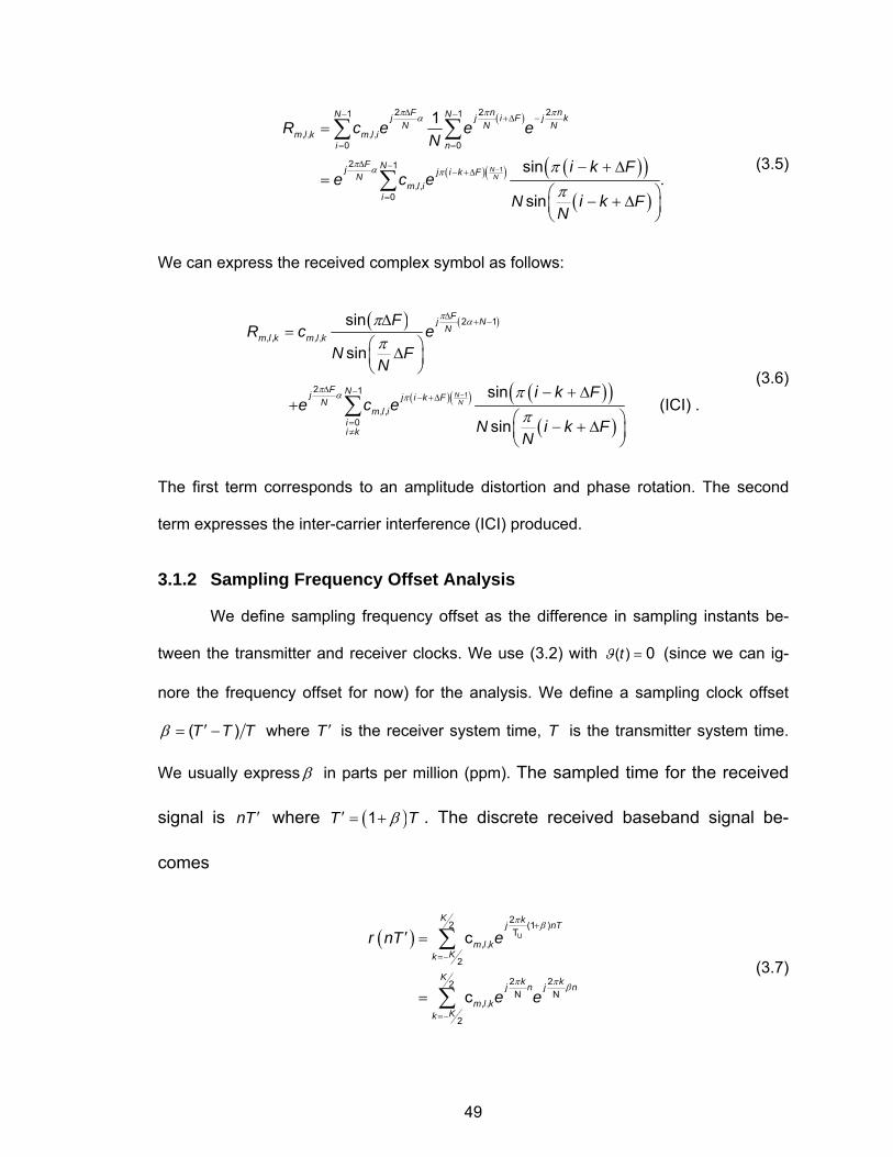
49

( )

( )( ) ( )( )( )

π π πα

π α π ππ

−

Δ− − +Δ −

= =

Δ −− +Δ

=

=

− + Δ=

⎛ ⎞− + Δ⎜ ⎟⎝ ⎠

∑ ∑

∑1

2 2 21 1

, , , ,0 0

2 1

, ,0

1

sin.

sin

NN

F n nN Nj j i F j kN N N

m l k m l ii n

F Nj j i k FNm l i

i

R c e e eN

i k Fe c e

N i k FN

(3.5)

We can express the received complex symbol as follows:

( ) ( )

( )( ) ( )( )( )

π α

π α π

ππ

ππ

−

Δ+ −

Δ −− +Δ

=≠

Δ=

⎛ ⎞Δ⎜ ⎟⎝ ⎠

− + Δ+

⎛ ⎞− + Δ⎜ ⎟⎝ ⎠

∑1

2 1

, , , ,

2 1

, ,0

sin

sin

sin(ICI) .

sin

NN

Fj NN

m l k m l k

F Nj j i k FNm l i

ii k

FR c e

N FN

i k Fe c e

N i k FN

(3.6)

The first term corresponds to an amplitude distortion and phase rotation. The second

term expresses the inter-carrier interference (ICI) produced.

3.1.2 Sampling Frequency Offset Analysis

We define sampling frequency offset as the difference in sampling instants be-

tween the transmitter and receiver clocks. We use (3.2) with ϑ =( ) 0t (since we can ig-

nore the frequency offset for now) for the analysis. We define a sampling clock offset

β ′= −( )T T T where ′T is the receiver system time, T is the transmitter system time.

We usually express β in parts per million (ppm). The sampled time for the received

signal is ′nT where ( )β′ = +1T T . The discrete received baseband signal be-

comes

( ) U

22 (1 )T

, ,

2

2 22N N

, ,

2

c

c

K kj nT

m l kKk

K k kj n j n

m l kKk

r nT e

e e

π β

π π β

+

=−

=−

′ =

=

∑

∑ (3.7)

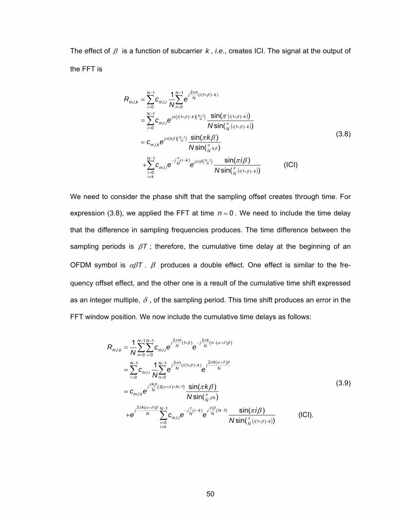
50

The effect of β is a function of subcarrier k , i.e., creates ICI. The signal at the output of

the FFT is

( )( )( ) ( )( )( )( )

( )( )

( ) ( )( )( )

1

1

1

21 1 ( (1 ) )

, , , ,0 01

11, ,

10

, ,

1

, ,10

1

sin( )sin( )

sin( ) sin( )

sin( ) (ICIsin( )

NN

NN

NN

nN N j i kN

m l k m l ii n

Ni kj i k

m l ii ki N

j km l k

kN

N j i k j iNm l i

i ki Ni k

R c eN

c eNkc e

N

ic e eN

π β

βπ βπ

β

π βπ

β

ππ β

πβ

π

π β

π β

−

−

−

− − + −

= =

−+ −+ −

+ −=

− − −

+ −=≠

=

=

=

+

∑ ∑

∑

∑ )

(3.8)

We need to consider the phase shift that the sampling offset creates through time. For

expression (3.8), we applied the FFT at time = 0n . We need to include the time delay

that the difference in sampling frequencies produces. The time difference between the

sampling periods is βT ; therefore, the cumulative time delay at the beginning of an

OFDM symbol is αβT . β produces a double effect. One effect is similar to the fre-

quency offset effect, and the other one is a result of the cumulative time shift expressed

as an integer multiple, δ , of the sampling period. This time shift produces an error in the

FFT window position. We now include the cumulative time delays as follows:

( )( )

( )

( )( )

( ) ( ) ( )

2 21 1 (1 )

, , , ,0 0

221 1 ( (1 ) )

, ,0 0

2 1

, ,

2 1 1

, ,0

1

1

sin( )sin( )

sin( )sin(

ni kN N j j nN N

m l k m l in i

knN N j i k jN N

m l ii n

kj NN

m l kkN

k iNj j i k j NN N N

m l iii k

R c e eN

c e eN

kc eN

ie c e eN

π πβ α δ β

π α δ βπ β

π β α δ

πβ

π α δ β π π β

π

π β

π β

− − + − − +

= =

+− − + −

= =

+ + −

+ − − − −

=≠

=

=

=

+

∑∑

∑ ∑

∑( )( )1

(ICI).)i kN β+ −

(3.9)

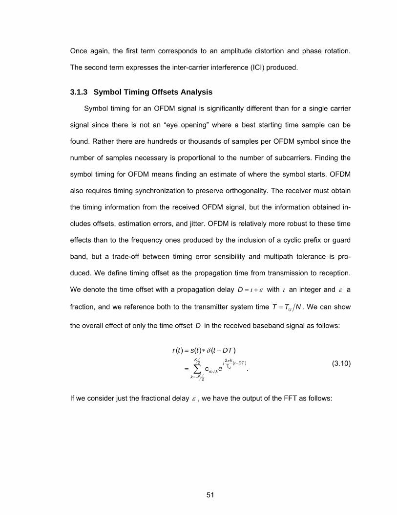
51

Once again, the first term corresponds to an amplitude distortion and phase rotation.

The second term expresses the inter-carrier interference (ICI) produced.

3.1.3 Symbol Timing Offsets Analysis

Symbol timing for an OFDM signal is significantly different than for a single carrier

signal since there is not an “eye opening” where a best starting time sample can be

found. Rather there are hundreds or thousands of samples per OFDM symbol since the

number of samples necessary is proportional to the number of subcarriers. Finding the

symbol timing for OFDM means finding an estimate of where the symbol starts. OFDM

also requires timing synchronization to preserve orthogonality. The receiver must obtain

the timing information from the received OFDM signal, but the information obtained in-

cludes offsets, estimation errors, and jitter. OFDM is relatively more robust to these time

effects than to the frequency ones produced by the inclusion of a cyclic prefix or guard

band, but a trade-off between timing error sensibility and multipath tolerance is pro-

duced. We define timing offset as the propagation time from transmission to reception.

We denote the time offset with a propagation delay ι ε= +D with ι an integer and ε a

fraction, and we reference both to the transmitter system time = UT T N . We can show

the overall effect of only the time offset D in the received baseband signal as follows:

U

22 ( )T

, ,

2

( ) ( ) ( )

c .K kj t DT

m l kKk

r t s t t DT

eπ

δ

−

=−

= ∗ −

= ∑ (3.10)

If we consider just the fractional delay ε , we have the output of the FFT as follows:

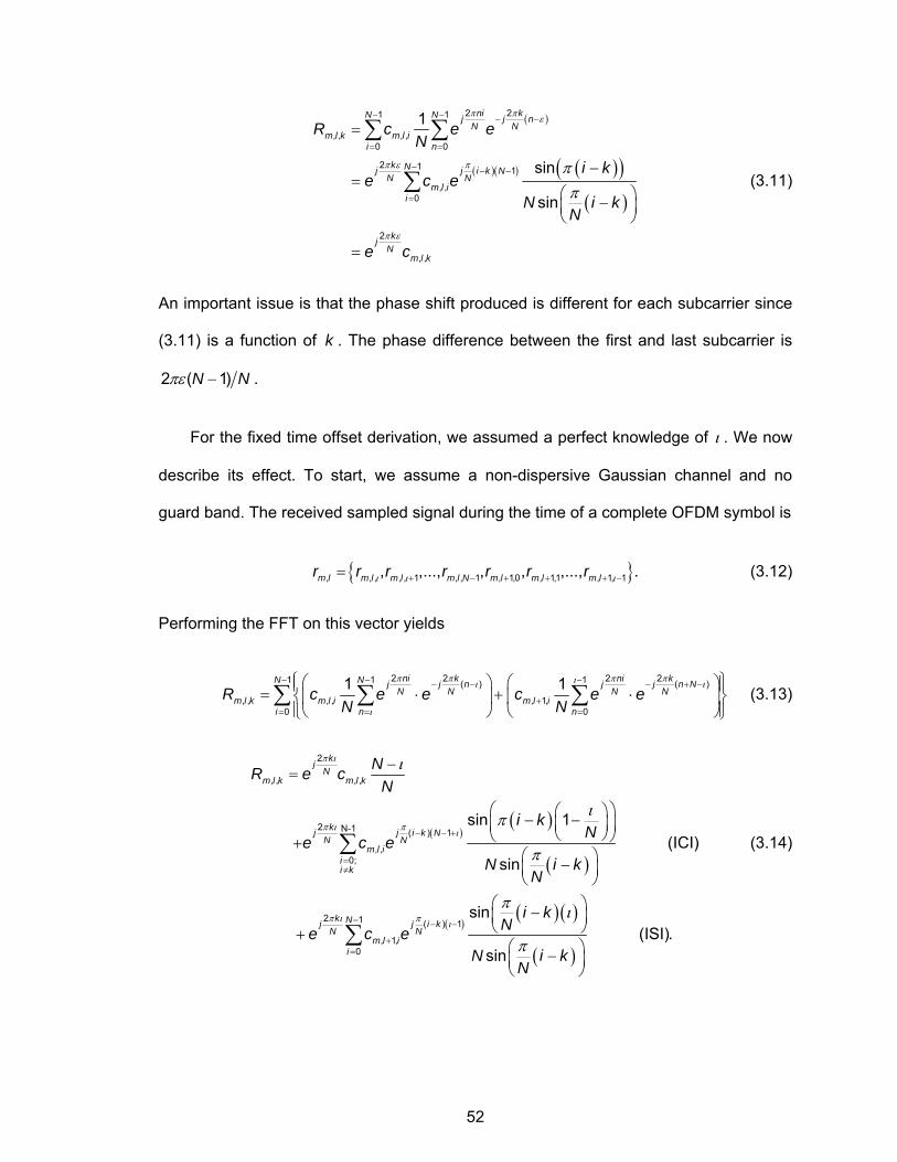
52

( )

( )( ) ( )( )( )

π π ε

π ε π

π ε

ππ

− − − −

= =

− − −

=

=

−=

⎛ ⎞−⎜ ⎟⎝ ⎠

=

∑ ∑

∑

2 21 1

, , , ,0 0

2 1 1

, ,0

2

, ,

1

sin

sin

ni kN N j j nN N

m l k m l ii n

k Nj j i k NN N

m l ii

kjN

m l k

R c e eN

i ke c e

N i kN

e c

(3.11)

An important issue is that the phase shift produced is different for each subcarrier since

(3.11) is a function of k . The phase difference between the first and last subcarrier is

πε −2 ( 1)N N .

For the fixed time offset derivation, we assumed a perfect knowledge of ι . We now

describe its effect. To start, we assume a non-dispersive Gaussian channel and no

guard band. The received sampled signal during the time of a complete OFDM symbol is

{ }ι ι ι+ − + + + −=, , , , , 1 , , 1 , 1,0 , 1,1 , 1, 1, ,..., , , ,..., .m l m l m l m l N m l m l m lr r r r r r r (3.12)

Performing the FFT on this vector yields

π π π πιι ι

ι

− − −− − − + −

+= = =

⎧ ⎫⎛ ⎞ ⎛ ⎞⎪ ⎪= ⋅ + ⋅⎨ ⎬⎜ ⎟ ⎜ ⎟⎪ ⎪⎝ ⎠ ⎝ ⎠⎩ ⎭

∑ ∑ ∑2 2 2 21 1 1( ) ( )

, , , , , 1,0 0

1 1ni k ni kN N j j n j j n NN N N N

m l k m l i m l ii n n

R c e e c e eN N

(3.13)

( )

( )

( )

( )( ) ( )

( )

2

, , , ,

2 N-1 ( ) 1

, ,0;

2 1 ( ) 1

, 1,0

sin 1(ICI)

sin

sin(ISI).

sin

kjN

m l k m l k

kj j i k NN N

m l iii k

k Nj j i kN N

m l ii

NR e cN

i kNe c e

N i kN

i kNe c e

N i kN

π ι

π ι π ι

π ι π ι

ι

ιπ

π

π ι

π

− − +

=≠

− − −

+=

−=

⎛ ⎞⎛ ⎞− −⎜ ⎟⎜ ⎟⎝ ⎠⎝ ⎠+⎛ ⎞−⎜ ⎟⎝ ⎠

⎛ ⎞−⎜ ⎟⎝ ⎠+⎛ ⎞−⎜ ⎟⎝ ⎠

∑

∑

(3.14)

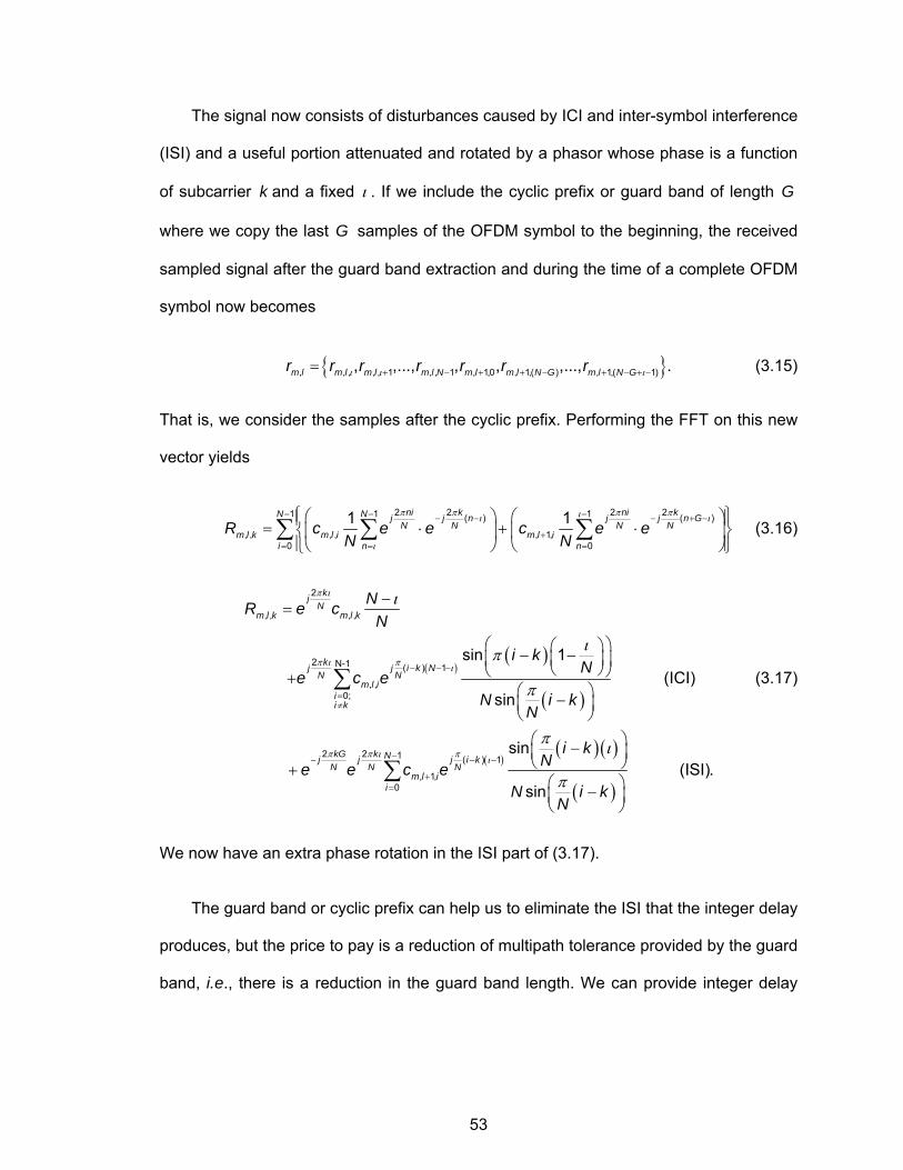
53

The signal now consists of disturbances caused by ICI and inter-symbol interference

(ISI) and a useful portion attenuated and rotated by a phasor whose phase is a function

of subcarrier k and a fixed ι . If we include the cyclic prefix or guard band of length G

where we copy the last G samples of the OFDM symbol to the beginning, the received

sampled signal after the guard band extraction and during the time of a complete OFDM

symbol now becomes

{ }ι ι ι+ − + + − + − + −=, , , , , 1 , , 1 , 1,0 , 1,( ) , 1,( 1), ,..., , , ,..., .m l m l m l m l N m l m l N G m l N Gr r r r r r r (3.15)

That is, we consider the samples after the cyclic prefix. Performing the FFT on this new

vector yields

π π π πιι ι

ι

− − −− − − + −

+= = =

⎧ ⎫⎛ ⎞ ⎛ ⎞⎪ ⎪= ⋅ + ⋅⎨ ⎬⎜ ⎟ ⎜ ⎟⎪ ⎪⎝ ⎠ ⎝ ⎠⎩ ⎭

∑ ∑ ∑2 2 2 21 1 1( ) ( )

, , , , , 1,0 0

1 1ni k ni kN N j j n j j n GN N N N

m l k m l i m l ii n n

R c e e c e eN N

(3.16)

( )

( )

( )

( )( ) ( )

( )

2

, , , ,

2 N-1 ( ) 1

, ,0;

2 2 1 ( ) 1

, 1,0

sin 1(ICI)

sin

sin(ISI).

sin

kjN

m l k m l k

kj j i k NN N

m l iii k

kG k Nj j j i kN N N

m l ii

NR e cN

i kNe c e

N i kN

i kNe e c e

N i kN

π ι

π ι π ι

π π ι π ι

ι

ιπ

π

π ι

π

− − −

=≠

−− − −

+=

−=

⎛ ⎞⎛ ⎞− −⎜ ⎟⎜ ⎟⎝ ⎠⎝ ⎠+⎛ ⎞−⎜ ⎟⎝ ⎠⎛ ⎞−⎜ ⎟⎝ ⎠+⎛ ⎞−⎜ ⎟⎝ ⎠

∑

∑

(3.17)

We now have an extra phase rotation in the ISI part of (3.17).

The guard band or cyclic prefix can help us to eliminate the ISI that the integer delay

produces, but the price to pay is a reduction of multipath tolerance provided by the guard

band, i.e., there is a reduction in the guard band length. We can provide integer delay

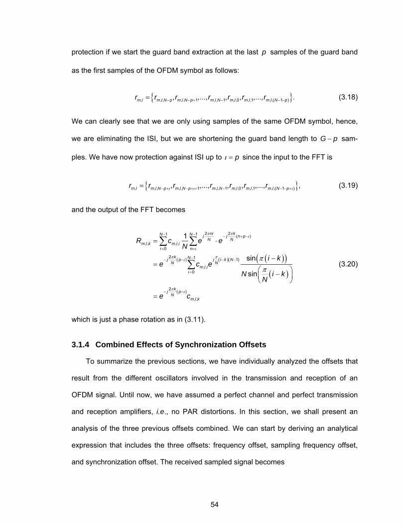
54

protection if we start the guard band extraction at the last p samples of the guard band

as the first samples of the OFDM symbol as follows:

{ }− − + − − −=, , , , , 1 , , 1 , ,0 , ,1 , ,( 1 ), ,..., , , ,..., .m l m l N p m l N p m l N m l m l m l N pr r r r r r r (3.18)

We can clearly see that we are only using samples of the same OFDM symbol, hence,

we are eliminating the ISI, but we are shortening the guard band length to −G p sam-

ples. We have now protection against ISI up to ι = p since the input to the FFT is

{ }ι ι ι− + − + + − − − +=, , , , , 1 , , 1 , ,0 , ,1 , ,( 1 ), ,..., , , ,..., ,m l m l N p m l N p m l N m l m l m l N pr r r r r r r (3.19)

and the output of the FFT becomes

( ) ( )( ) ( )( )

( )

( )

π π ι

ι

π πι

π ι

ππ

− − − + −

= =

−− − − −

=

− −

= ⋅

−=

⎛ ⎞−⎜ ⎟⎝ ⎠

=

∑ ∑

∑

2 21 1 ( )

, , , ,0

2 1 1

, ,0

2

, ,

1

sin

sin

ni kN N j j n pN N

m l k m l ii n

k Nj p j i k NN N

m l ii

kj pN

m l k

R c e eN

i ke c e

N i kN

e c

(3.20)

which is just a phase rotation as in (3.11).

3.1.4 Combined Effects of Synchronization Offsets

To summarize the previous sections, we have individually analyzed the offsets that

result from the different oscillators involved in the transmission and reception of an

OFDM signal. Until now, we have assumed a perfect channel and perfect transmission

and reception amplifiers, i.e., no PAR distortions. In this section, we shall present an

analysis of the three previous offsets combined. We can start by deriving an analytical

expression that includes the three offsets: frequency offset, sampling frequency offset,

and synchronization offset. The received sampled signal becomes

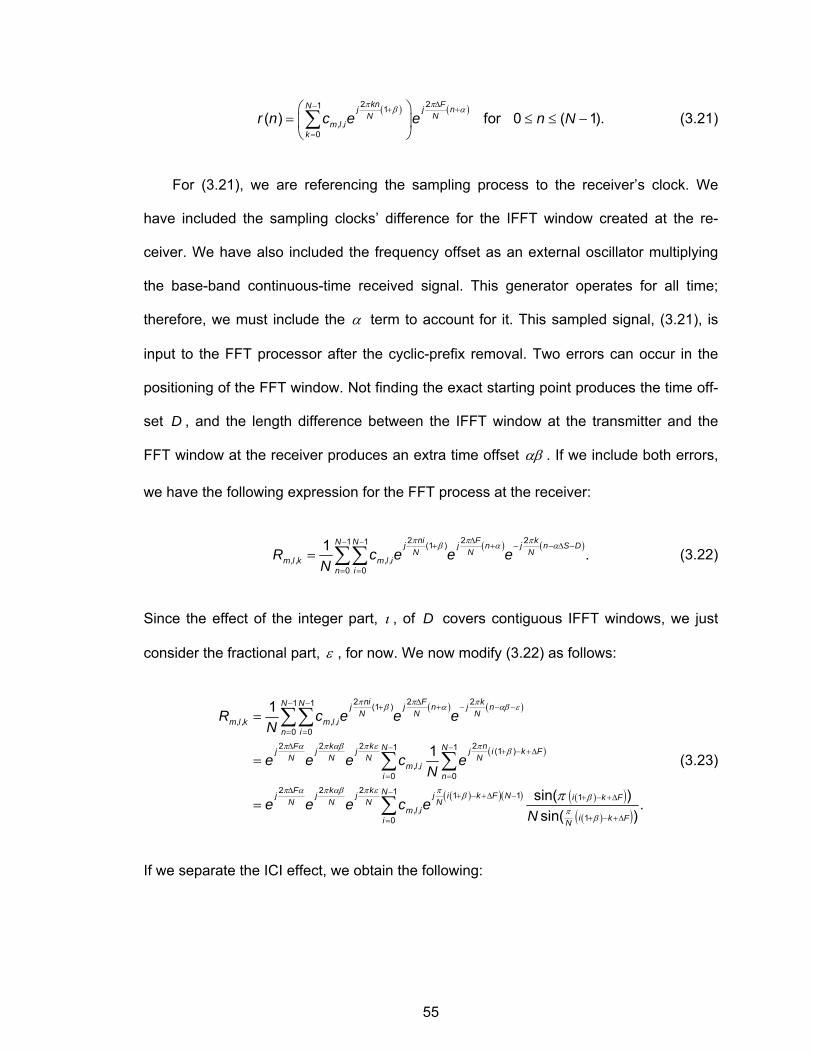
55

( ) ( )2 21 1

, ,0

( ) for 0 ( 1).kn FN j j n

N Nm l i

kr n c e e n N

π πβ αΔ− + +

=

⎛ ⎞= ≤ ≤ −⎜ ⎟⎝ ⎠∑ (3.21)

For (3.21), we are referencing the sampling process to the receiver’s clock. We

have included the sampling clocks’ difference for the IFFT window created at the re-

ceiver. We have also included the frequency offset as an external oscillator multiplying

the base-band continuous-time received signal. This generator operates for all time;

therefore, we must include the α term to account for it. This sampled signal, (3.21), is

input to the FFT processor after the cyclic-prefix removal. Two errors can occur in the

positioning of the FFT window. Not finding the exact starting point produces the time off-

set D , and the length difference between the IFFT window at the transmitter and the

FFT window at the receiver produces an extra time offset αβ . If we include both errors,

we have the following expression for the FFT process at the receiver:

( ) ( )2 2 21 1 (1 )

, , , ,0 0

1 .ni F kN N j j n j n S D

N N Nm l k m l i

n iR c e e e

N

π π πβ α αΔ− − + + − − Δ −

= =

= ∑∑ (3.22)

Since the effect of the integer part, ι , of D covers contiguous IFFT windows, we just

consider the fractional part, ε , for now. We now modify (3.22) as follows:

( ) ( )

( )

( )( )( ) ( )( )

2 2 21 1 (1 )

, , , ,0 0

2 2 2 21 1 (1 )

, ,0 0

2 2 2 1 1 1 1, ,

0

1

1

sin( )sin(

ni F kN N j j n j nN N N

m l k m l in i

F k k nN Nj j j j i k FN N N N

m l ii n

F k k Nj j j j i k F N i k FN N N Nm l i

i

R c e e eN

e e e c eN

e e e c eN

π π πβ α αβ ε

π α π αβ π ε π β

π α π αβ π ε π β βπ

Δ− − + + − − −

= =

Δ − − + − +Δ

= =

Δ − + − +Δ − + − +Δ

=

=

=

=

∑∑

∑ ∑

∑( )( )1

.)i k FN

πβ+ − +Δ

(3.23)

If we separate the ICI effect, we obtain the following:

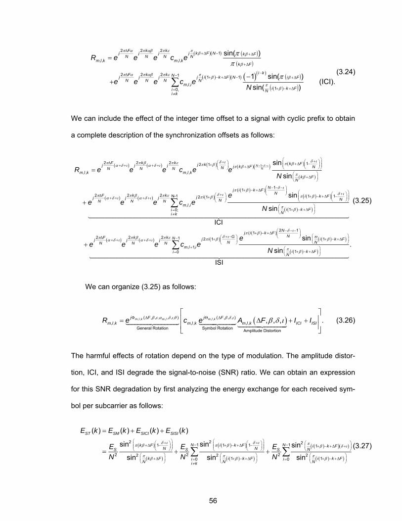
56

( )( ) ( )( )

( )( )( ) ( )( ) ( )

( )( )

2 2 2 1

, , , ,

2 2 2 1 1 1

, ,10,

sin( )

1 sin( )(ICI).

sin( )

F k kj j j j k F N k FN N N Nm l k m l k

k F

i kF k k Nj j j j i k F N i FN N N N

m l ii k Fi N

i k

R e e e c e

e e e c eN

π α π αβ π ε π β β

β

π α π αβ π ε π β β

πβ

ππ

π

Δ+Δ − +Δ

+Δ

−Δ − + − +Δ − +Δ

+ − +Δ=≠

=

−+ ∑

(3.24)

We can include the effect of the integer time offset to a signal with cyclic prefix to obtain

a complete description of the synchronization offsets as follows:

( ) ( ) ( ) ( )( ) ( )

( )

( ) ( ) ( )( )

δ ιδ ιδ ιπ π β π ε π βπ βα δ ι α δ ι π β

π β

δπ βδ ιπ π β π ε π βα δ ι α δ ι

− − −

⎛ ⎞+⎛ ⎞+⎛ ⎞Δ ⎜ ⎟+Δ −+ ⎜ ⎟⎜ ⎟+ + + + ⎜ ⎟ +Δ ⎝ ⎠⎝ ⎠⎝ ⎠⎛ ⎞

+Δ⎜ ⎟⎝ ⎠

− − −+ − +Δ

+⎛ ⎞Δ ++ + + + ⎜ ⎟⎝ ⎠

=

+

12 2 2 12 1

, , , ,

1( 1 )2 2 2 2 1

, ,

sin

sin

NN

F k k k Fj kj j j j k F NNN N Nm l k m l k

k FN

Nj i k FF k k j ij j j NN N N

m l i

R e e e c e eN

ee e e c e

( )( )

( )( )

( ) ( )

ιδ ιπ β

π β

π π β π εα δ ι α δ ι

⎛ ⎞⎜ ⎟ ⎛ ⎞+⎝ ⎠ ⎛ ⎞⎜ ⎟+ − +Δ −⎜ ⎟⎜ ⎟⎝ ⎠⎝ ⎠

⎛ ⎞+ − +Δ⎜ ⎟=

⎝ ⎠≠

Δ+ + + +

++

∑N-1 1 1

10;

2 2 2

, 1,

ICI

sin

sin

Ni k F

N

i k FiNi k

F k kj j jN N N

m l

N

e e e c( )

( )( )( )

( )( )

δ ιπ βπιδ ι βπ β

π β

− − −⎛ ⎞+ − +Δ ⎜ ⎟ ⎛ ⎞+ − ⎝ ⎠⎛ ⎞− + − +Δ+ ⎜ ⎟⎜ ⎟ ⎝ ⎠⎝ ⎠⎛ ⎞

+ − +Δ⎜ ⎟=⎝ ⎠

∑

2 1( 1 )1 12 1

10

ISI

sin.

sin

Nj i k FNGN i k Fj i

NNi

i k FiN

ee

N

(3.25)

We can organize (3.25) as follows:

( )β ε α δ ι θ β δ ι β δ ιΦ Δ Θ Δ⎡ ⎤⎢ ⎥= Δ + +⎢ ⎥⎣ ⎦

, , , , ,( , , , , , , ) ( , , , ), , , , , ,

General Rotation Symbol Rotation Amplitude Distortion

, , , .m l k m l m l kj F j Fm l k m l k m l k ICI ISIR e c e A F I I (3.26)

The harmful effects of rotation depend on the type of modulation. The amplitude distor-

tion, ICI, and ISI degrade the signal-to-noise (SNR) ratio. We can obtain an expression

for this SNR degradation by first analyzing the energy exchange for each received sym-

bol per subcarrier as follows:

( )

( )

( )( )

( )( )

( )( )( )

( )( )

2 2 211 1 1 1

2 2 22 2 21 10

( ) ( ) ( ) ( )

sin sin sin

sin sin sin

ST SM SICI SISI

Nk F i k F i k FN N NS S S

k F i k F i k FiN N N

E k E k E k E k

E E EN N N

δ ι δ ι ππ β π β β δ ι

π π πβ β β

⎛ ⎞ ⎛ ⎞+ + ⎛ ⎞⎛ ⎞ ⎛ ⎞⎜ ⎟ ⎜ ⎟ −+Δ − + − +Δ − + − +Δ +⎜ ⎟ ⎜ ⎟ ⎜ ⎟⎜ ⎟ ⎜ ⎟⎝ ⎠ ⎝ ⎠⎝ ⎠ ⎝ ⎠ ⎝ ⎠⎛ ⎞ ⎛ ⎞ ⎛ ⎞

+Δ + − +Δ + − +Δ⎜ ⎟ ⎜ ⎟ ⎜ ⎟=⎝ ⎠ ⎝ ⎠ ⎝ ⎠

= + +

= + + ∑1

0

N

ii k

−

=≠

∑(3.27)

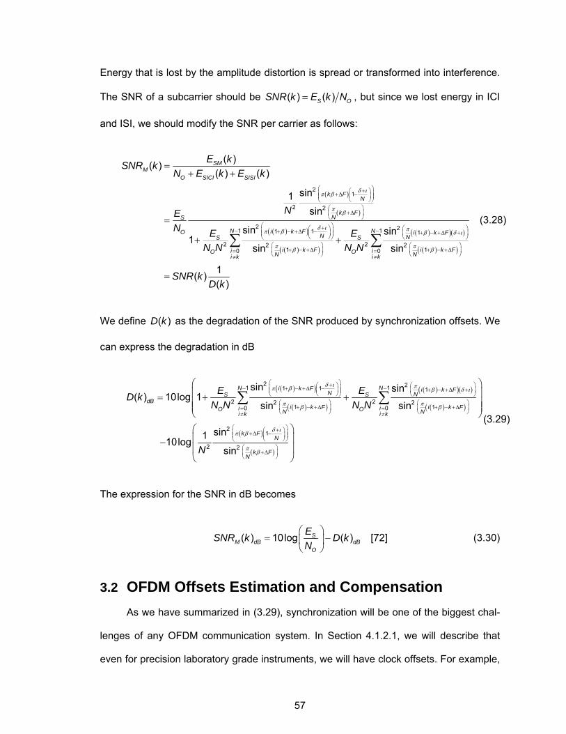
57

Energy that is lost by the amplitude distortion is spread or transformed into interference.

The SNR of a subcarrier should be ( ) ( )S OSNR k E k N= , but since we lost energy in ICI

and ISI, we should modify the SNR per carrier as follows:

( )

( )

( )( )

( )( )

( )( )( )

21

2 2

2 21 1 1 1

2 22 210

( )( )( ) ( )

sin1sin

sin sin1

sin sin

SMM

O SICI SISI

k FN

k FNS

N i k FO i k FN NS S

i k F iiO ON Ni k

E kSNR kN E k E k

NEN E E

N N N N

δ ιπ β

π β

δ ι ππ β β δ ι

π πβ

⎛ ⎞+⎛ ⎞⎜ ⎟+Δ −⎜ ⎟⎜ ⎟⎝ ⎠⎝ ⎠⎛ ⎞

+Δ⎜ ⎟⎝ ⎠

⎛ ⎞+ ⎛ ⎞⎛ ⎞⎜ ⎟− + − +Δ − + − +Δ +⎜ ⎟ ⎜ ⎟⎜ ⎟⎝ ⎠⎝ ⎠ ⎝ ⎠⎛ ⎞

+ − +Δ⎜ ⎟= ⎝ ⎠≠

=+ +

=

+ +∑( )( )

1

10

1( )( )

N

k Fii k

SNR kD k

β

−

⎛ ⎞+ − +Δ⎜ ⎟= ⎝ ⎠≠

=

∑(3.28)

We define ( )D k as the degradation of the SNR produced by synchronization offsets. We

can express the degradation in dB

( )( )

( )( )

( )( )( )

( )( )

( )

2 21 11 1 1

2 22 21 10 0

21

2 2

sin sin( ) 10log 1

sin sin

sin110logsin

N Ni k F i k FN NS SdB

i k F i k Fi iO ON Ni k i k

k FN

E ED kN N N N

N

δ ι ππ β β δ ι

π πβ β

δ ιπ β

⎛ ⎞+ ⎛ ⎞⎛ ⎞⎜ ⎟− −+ − +Δ − + − +Δ +⎜ ⎟ ⎜ ⎟⎜ ⎟⎝ ⎠⎝ ⎠ ⎝ ⎠⎛ ⎞ ⎛ ⎞

+ − +Δ + − +Δ⎜ ⎟ ⎜ ⎟= =⎝ ⎠ ⎝ ⎠≠ ≠

⎛ ⎞+⎛ ⎞⎜ ⎟+Δ −⎜ ⎟⎜ ⎟⎝ ⎠⎝ ⎠

⎛ ⎞⎜ ⎟= + +⎜ ⎟⎜ ⎟⎝ ⎠

−

∑ ∑

( )k FNπ β

⎛ ⎞+Δ⎜ ⎟

⎝ ⎠

⎛ ⎞⎜ ⎟⎜ ⎟⎝ ⎠

(3.29)

The expression for the SNR in dB becomes

( ) 10log ( )SM dB dB

O

ESNR k D kN

⎛ ⎞= −⎜ ⎟

⎝ ⎠[72] (3.30)

3.2 OFDM Offsets Estimation and Compensation As we have summarized in (3.29), synchronization will be one of the biggest chal-

lenges of any OFDM communication system. In Section 4.1.2.1, we will describe that

even for precision laboratory grade instruments, we will have clock offsets. For example,

58

in our particular setup, we derive the up/down conversion oscillator frequency from the

ADC clock, which we know has an offset compared to the transmitter clock that creates

a sampling frequency offset; therefore, there is also frequency offset. In this case, which

can easily be the case for many systems, we have no means of adjusting the clock fre-

quency in real time; therefore, we propose an off-line algorithm to detect FΔ ,ι ,ε , and

β to compensate via software.

As we described in Section 2.4, we can find a vast amount of information about

OFDM synchronization in the literature. Out of this information, we can propose two

categories for the detection algorithms: pre-FFT and post-FFT. In the former, the signal

is the sampled baseband signal where we can use some form of correlation of the

guard-band to detect FΔ and ι , and we have the frame separation signal to also detect

ι . In the latter, we can use the symbol rotation information to detect FΔ , β and ε .

Since our objective is a calibration procedure, our interest is in accuracy; therefore, we

propose using a combination of DA and NDA maximum-likelihood (ML) techniques. Out

of all the techniques in the literature, we have chosen the pre-FFT technique in [10], [70]

to detect FΔ and ι . This is a NDA technique since it uses the guard-band or cyclic pre-

fix interval. We now present a brief summary. The log-likelihood function is

( ) ( ) ( ), F m mι γ ρΛ Δ = − Φ (3.31)

where the correlation is

( ) ( ) ( )1

,m N

k mm r k r k Nγ

+ −∗

=

= +∑ (3.32)

the energy is

59

( ) ( ) ( )1 2 21 ,

2

m N

k mm r k r k N

+ −

=

Φ = + +∑ (3.33)

and

.1

SNRSNR

ρ =+

(3.34)

From this log-likelihood function, the estimates are

( ){ }( ){ }

ˆ argmin ,

ˆ .

ML

ML ML

F

F angle

ι ι

γ ι∧

= Λ Δ

Δ = (3.35)

Since all the post-FFT techniques rely on the measurement of the rotation angle of

the symbol at the output of the FFT, every parameter to detect adds a dimension to the

ML function; therefore, we should try to detect and correct as many parameters as pos-

sible before the FFT. So far, we have detected two of the four parameters that appear in

the symbol rotation. To detect the other two, we must compensate for the ones that we

have found. First, we multiply the baseband signal as follows:

( )2

( ) ( ) ,Fj n

Nr n r n eπ α

∧Δ

− +=% (3.36)

and then, we use ι to correctly start the FFT window. We have reduced the synchroni-

zation distortion to:

( )

( )( )( ) ( )( )

( )( )

π παβ ε π β

π βπ παβ ε

πβ

π βπ β

π β

−

− −+ −−

+ −=≠

=

−+ +∑

1

1

2 2

, , , ,

12 2 1

, , , ,10,

sin( )

1 sin( ) .

sin( )

NN

NN

j k j k j kN Nm l k m l k

i kj i kNj k j kN N

m l i m l ki ki Ni k

ICI

kR e e c ek

iee e c WN

(3.37)

60

We now present a post-FFT DA technique to detect the last two parameters. We

suggest using a frame of L OFDM symbols for this purpose. The technique is a modifica-

tion of [24], [41], [73], [76], [77]. The log-likelihood function given a set of parameters

{ }1, , , ,l kc ε β , with non-random offsets, for an AWGN channel is

{ }00

2 ( ) ( )T

r t s t dtN

∗Λ = ℜ∫ (3.38)

From (3.38), the ML estimates are

( )( )

( )( )1, , 1, , 1, ,, 0, , 1

ˆˆ, argmin ln , ,

l k l k l Lx y k N

p R x y cε β ε β == −

⎧ ⎫⎡ ⎤= = =⎨ ⎬⎢ ⎥

⎣ ⎦⎩ ⎭KK (3.39)

(3.39) implies that we have to minimize the expression 2

1, 1,1

Ll ll=−∑ R T where we define

the components of the vector 1,lT as 1,

2 12

1, , 1, ,

lNj k x y

Nl k l kT c e

π α⎛ ⎞−⎛ ⎞− + +⎜ ⎟⎜ ⎟⎝ ⎠⎝ ⎠= . We expand the square

norm to obtain

( )

1,2 11 22 2

1, , 1, , 1, , 1, ,1 0

independent of ,

2 .l

NL N j k x yN

l k l k l k l kl k

x y

R T R c eπ α⎛ ⎞−⎛ ⎞− − + +⎜ ⎟⎜ ⎟∗ ⎝ ⎠⎝ ⎠

= =

⎡ ⎤⎛ ⎞⎢ ⎥⎜ ⎟+ − ℜ⎢ ⎥⎜ ⎟⎝ ⎠⎢ ⎥⎣ ⎦

∑∑ 1 44 2 4 43 (3.40)

The ML estimates expression becomes

( )( )

2 12

1, , 1, ,, 1

ˆˆ, argminNL K j k x y

Nl k l k

x y l k KR c e

π αε β

⎛ ⎞−⎛ ⎞− + +⎜ ⎟⎜ ⎟∗ ⎝ ⎠⎝ ⎠

= =−

⎧ ⎫⎡ ⎤⎛ ⎞⎪ ⎪⎢ ⎥⎜ ⎟= − ℜ⎨ ⎬⎜ ⎟⎢ ⎥⎪ ⎪⎝ ⎠⎣ ⎦⎩ ⎭∑ ∑ (3.41)

from which we define a function to minimize as

61

2 1

21, , 1, ,

1( , ) .

NL K j k x yN

l k l kl k K

F x y R c eπ α⎛ ⎞−⎛ ⎞− + +⎜ ⎟⎜ ⎟∗ ⎝ ⎠⎝ ⎠

= =−

⎡ ⎤⎛ ⎞⎢ ⎥⎜ ⎟= ℜ

⎜ ⎟⎢ ⎥⎝ ⎠⎣ ⎦∑ ∑ (3.42)

There are many computer programs available for this classical two-dimensional

minimization problem, but we will present a differential procedure that transforms the

problem into a one-dimensional case. We can start by using a simplified expression for

(3.36) as follows:

1, , 1, , +(ICI)+( )jAl k l kR c e noise≅ (3.43)

Now, let us multiply this symbol by the conjugate of the previous symbol as shown:

( )

1, , 1, 1, 1, , 1 1 1, 1, 2 2

1, , 1, 1,

+(ICI )+( ) +(ICI )+( )

.

jA jBl k l k l k l k

j A Bl k l k

R R c e noise c e noise

c c e NOISE

∗ ∗ −− −

−∗−

⎡ ⎤ ⎡ ⎤≅ ⎣ ⎦ ⎣ ⎦

= + (3.44)

If we look only at the exponent

( )

1, 1, 1

1, 1, 1

2 1 2 12 2

2 ,

l l

l l

k N k NA BN N

kN

π πε α β ε α β

π β α α

−

−

⎛ ⎞ ⎛ ⎞− −⎛ ⎞ ⎛ ⎞− = + + − + +⎜ ⎟ ⎜ ⎟⎜ ⎟ ⎜ ⎟⎝ ⎠ ⎝ ⎠⎝ ⎠ ⎝ ⎠

= −

(3.45)

we can see that we have gotten rid of the time-offset term ε . We have now to estimate

just one parameter. We define , , , , , 1,m l k m l k m l kQ R R∗−= , , , , , , 1,m l k m l k m l kS c c∗

−= , and

, , , , , ,m l k m l k m l kZ Q S∗= , and the ML expression becomes

( ), , 1

2

, ,2

( ) m l m lkyL K j

Nm l k

l k KF y Z e

π α α −− −

= =−

⎛ ⎞= − ℜ⎜ ⎟

⎝ ⎠∑ ∑ (3.46)

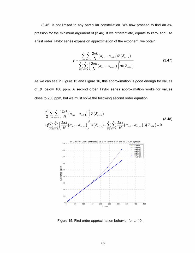
62

(3.46) is not limited to any particular constellation. We now proceed to find an ex-

pression for the minimum argument of (3.46). If we differentiate, equate to zero, and use

a first order Taylor series expansion approximation of the exponent, we obtain:

( ) ( )

( ) ( )

, , 1 , ,2

2

, , 1 , ,2

2

ˆ2

L K

m l m l m l kl k K

L K

m l m l m l kl k K

k ZNyk Z

N

π α α

π α α

−= =−

−= =−

− ℑ≈

⎛ ⎞− ℜ⎜ ⎟⎝ ⎠

∑ ∑

∑ ∑ (3.47)

As we can see in Figure 15 and Figure 16, this approximation is good enough for values

of β below 100 ppm. A second order Taylor series approximation works for values

close to 200 ppm, but we must solve the following second order equation

( ) ( )

( ) ( ) ( ) ( )

32

, , 1 , ,2

2

, , 1 , , , , 1 , ,2 2

ˆ 22

2 2ˆ 0

L K

m l m l m l kl k K

L K L K

m l m l m l k m l m l m l kl k K l k K

y k ZN

k ky Z ZN N

π α α

π πα α α α

−= =−

− −= =− = =−

⎛ ⎞− ℑ⎜ ⎟⎝ ⎠

⎛ ⎞+ − ℜ − − ℑ =⎜ ⎟⎝ ⎠

∑ ∑

∑ ∑ ∑ ∑ (3.48)

0 50 100 150 200 250 300 350 400 4500

50

100

150

200

250

300

350

400

45064 QAM 1st Order Estimated β vs. β for various SNR and 10 OFDM Symbols

β ppm

Est

imat

ed β

ppm

SNR=5SNR=10SNR=15SNR=20SNR=25SNR=30True value

Figure 15: First order approximation behavior for L=10.

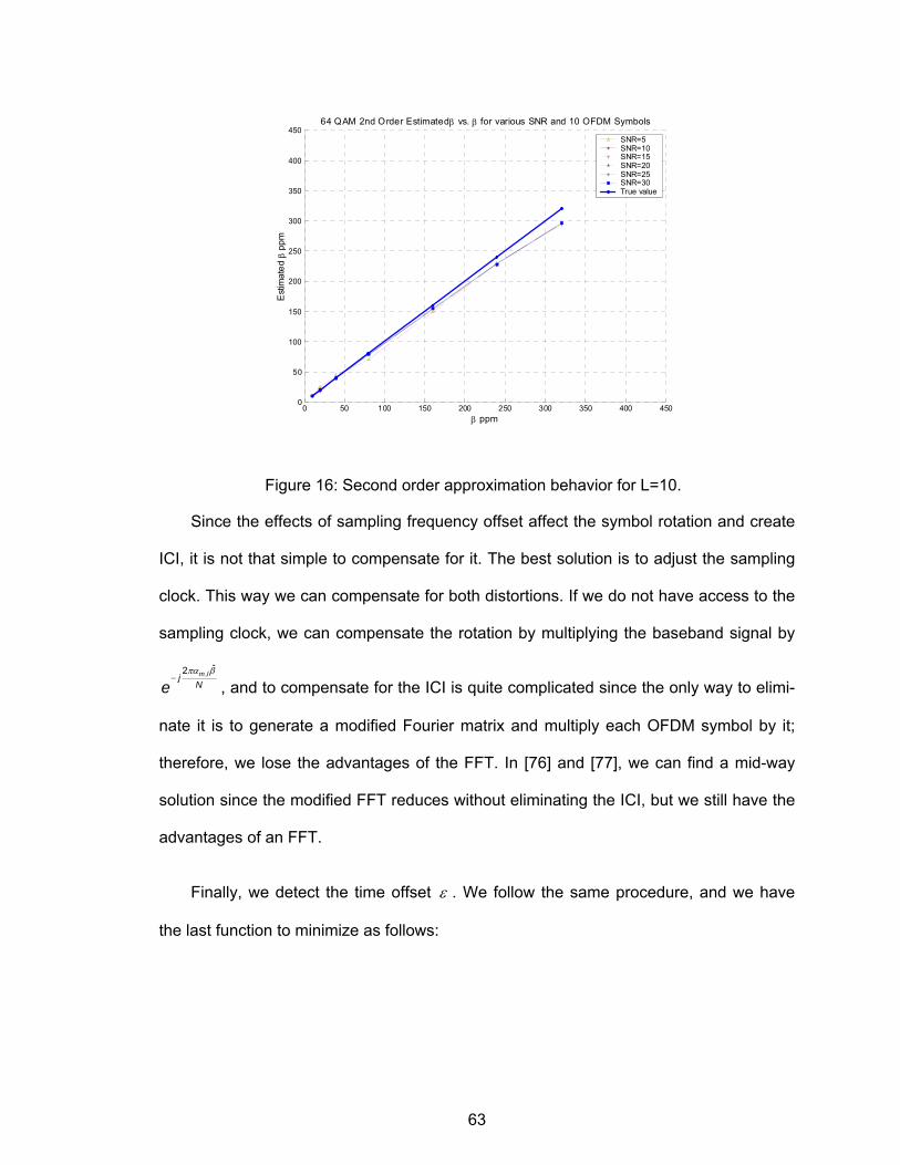
63

0 50 100 150 200 250 300 350 400 4500

50

100

150

200

250

300

350

400

45064 QAM 2nd Order Estimated β vs. β for various SNR and 10 OFDM Symbols

β ppm

Est

imat

ed β

ppm

SNR=5SNR=10SNR=15SNR=20SNR=25SNR=30True value

Figure 16: Second order approximation behavior for L=10.

Since the effects of sampling frequency offset affect the symbol rotation and create

ICI, it is not that simple to compensate for it. The best solution is to adjust the sampling

clock. This way we can compensate for both distortions. If we do not have access to the

sampling clock, we can compensate the rotation by multiplying the baseband signal by

,ˆ2 m lj

Neπα β

−, and to compensate for the ICI is quite complicated since the only way to elimi-

nate it is to generate a modified Fourier matrix and multiply each OFDM symbol by it;

therefore, we lose the advantages of the FFT. In [76] and [77], we can find a mid-way

solution since the modified FFT reduces without eliminating the ICI, but we still have the

advantages of an FFT.

Finally, we detect the time offset ε . We follow the same procedure, and we have

the last function to minimize as follows:

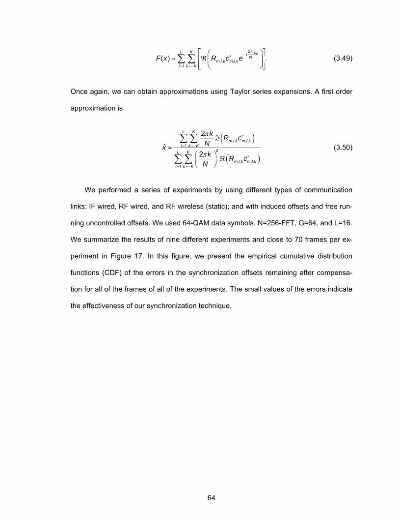
64

2

, , , ,1

( ) .L K j kx

Nm l k m l k

l k KF x R c e

π−∗

= =−

⎡ ⎤⎛ ⎞= ℜ⎢ ⎥⎜ ⎟

⎢ ⎥⎝ ⎠⎣ ⎦∑ ∑ (3.49)

Once again, we can obtain approximations using Taylor series expansions. A first order

approximation is

( )

( )

, , , ,1

2

, , , ,1

2

ˆ2

L K

m l k m l kl k K

L K

m l k m l kl k K

k R cNxk R c

N

π

π

∗

= =−

∗

= =−

ℑ≈

⎛ ⎞ ℜ⎜ ⎟⎝ ⎠

∑ ∑

∑ ∑ (3.50)

We performed a series of experiments by using different types of communication

links: IF wired, RF wired, and RF wireless (static); and with induced offsets and free run-

ning uncontrolled offsets. We used 64-QAM data symbols, N=256-FFT, G=64, and L=16.

We summarize the results of nine different experiments and close to 70 frames per ex-

periment in Figure 17. In this figure, we present the empirical cumulative distribution

functions (CDF) of the errors in the synchronization offsets remaining after compensa-

tion for all of the frames of all of the experiments. The small values of the errors indicate

the effectiveness of our synchronization technique.

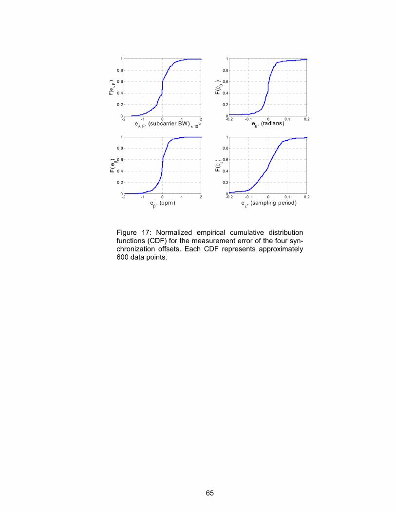
65

-2 -1 0 1 2

x 10-3

0

0.2

0.4

0.6

0.8

1

eΔ F, (subcarrier BW)

F(e Δ

F )

-0.2 -0.1 0 0.1 0.20

0.2

0.4

0.6

0.8

1

eθ, (radians)

F(eθ )

-2 -1 0 1 20

0.2

0.4

0.6

0.8

1

eβ, (ppm)

F( e

β)

-0.2 -0.1 0 0.1 0.20

0.2

0.4

0.6

0.8

1

eε, (sampling period)

F(e ε

)

Figure 17: Normalized empirical cumulative distribution functions (CDF) for the measurement error of the four syn-chronization offsets. Each CDF represents approximately 600 data points.

66

CHAPTER 4

CHANNEL MEASUREMENT SYSTEMS

The complete channel measurement campaign was performed at two different fre-

quency bands: 2.4 and 5.9 GHz. In each of this chapter’s sections, we will describe the

channel sounding system developed for a particular frequency band. We will indicate the

system’s specifications and limitations. We will also include a description and analysis of

the sounding waveform. We developed both systems by integrating available general

purpose equipment. As with any new system design, ours had some mistakes and er-

rors; therefore, we present an analysis of their effects, and how we managed to over-

come them.

4.1 2.4 GHz Channel Sounding System Development In this section, we present a detailed description of the design and performance of

our channel sounding system developed for the 2.4 GHz frequency band. For this pur-

pose, we also present a detailed analysis of the sounding waveform.

As shown on the right in Figure 18, an Agilent™ ESG E4438C RF signal generator

was used to create the MLS waveform of 511 chips, with the chip period of 50 ns, and a

3 dB bandwidth of approximately 20 MHz, centered at 2.445 GHz. The 511-chip burst

was repeated back-to-back, corresponding to a repetition period of 25.5 μs, which further

corresponds to a maximum unambiguous excess path length of 7.65 km and a maxi-

mum unambiguous Doppler shift of ±19.5 kHz. Following amplification and transmission

from a 8 dBi omnidirectional antenna mounted on the middle of the roof of a compact

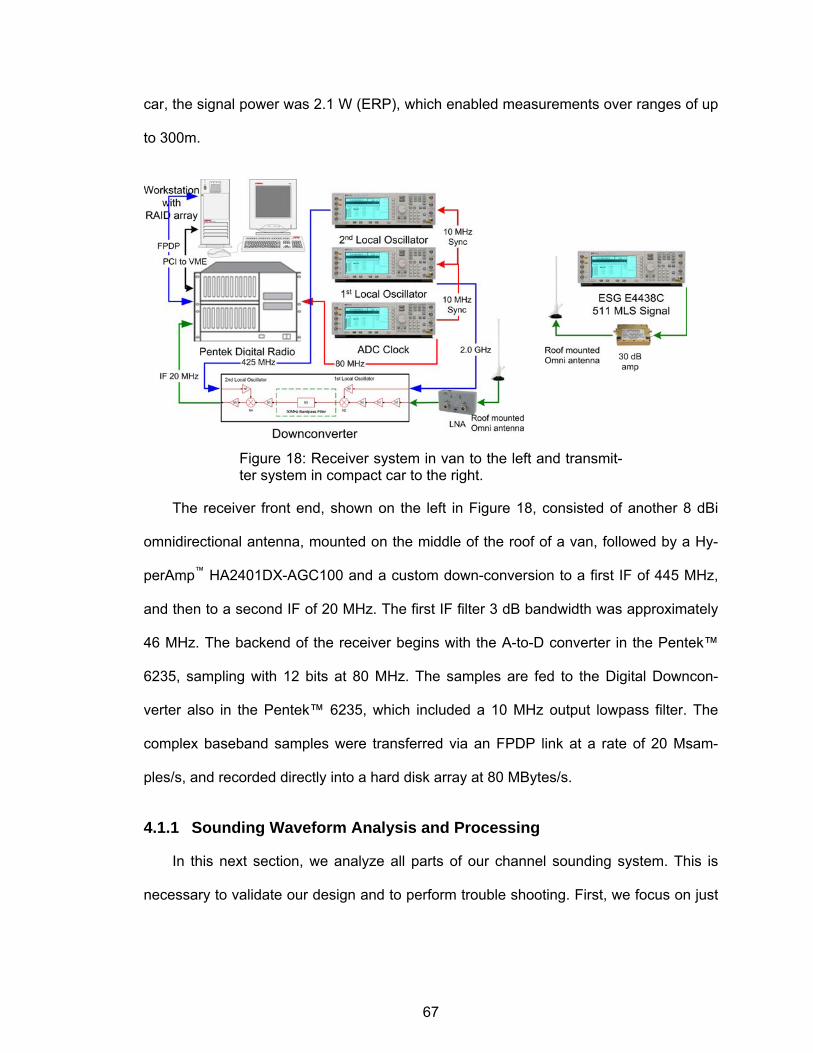
67

car, the signal power was 2.1 W (ERP), which enabled measurements over ranges of up

to 300m.

Figure 18: Receiver system in van to the left and transmit-ter system in compact car to the right.

The receiver front end, shown on the left in Figure 18, consisted of another 8 dBi

omnidirectional antenna, mounted on the middle of the roof of a van, followed by a Hy-

perAmp™ HA2401DX-AGC100 and a custom down-conversion to a first IF of 445 MHz,

and then to a second IF of 20 MHz. The first IF filter 3 dB bandwidth was approximately

46 MHz. The backend of the receiver begins with the A-to-D converter in the Pentek™

6235, sampling with 12 bits at 80 MHz. The samples are fed to the Digital Downcon-

verter also in the Pentek™ 6235, which included a 10 MHz output lowpass filter. The

complex baseband samples were transferred via an FPDP link at a rate of 20 Msam-

ples/s, and recorded directly into a hard disk array at 80 MBytes/s.

4.1.1 Sounding Waveform Analysis and Processing

In this next section, we analyze all parts of our channel sounding system. This is

necessary to validate our design and to perform trouble shooting. First, we focus on just

68

the transmitter and the receiver up to the IF output. Later, we continue with the analysis

of the sampling process and signal processing.

In the first part of the section, we present a complete analysis of the spectrum of our

sounding waveform. This analysis will enable us to detect irregularities or problems in

the system in real time using a spectrum analyzer. We analyze the spectrum three ways:

theoretically, through simulation and through measurement in a hardware implementa-

tion. The theoretical treatment derives the autocorrelation function of our probe wave-

form, and the transform of this to get the PSD of the waveform. We next compare the

theoretical PSD with that obtained from a SIMULINK™ simulation of the transmitter. Fi-

nally, we obtain measurements of the PSD at several points in the hardware implemen-

tation of the transmitter and receiver, for example one is from the RF output of the

transmitter and another is from the IF output of the receiver. We show that all of these

PSDs agree.

In the last part, we address the nonlinearities of the power amplifier and the receiver

low noise amplifier. It confirms that at the power levels of measurement, there should be

no intermodulation distortion in the recorded signal.

Since we are working with wideband signals modulated at 2.445 GHz, a spectrum

analyzer is the only available measurement equipment for passband signals; therefore,

we need a thorough understanding of the spectrum of our sounding waveform since this

way we will know the expected spectrum shape beforehand. This understanding will also

allow us to detect irregularities or problems in the system. In addition, we make exten-

sive use of simulations; therefore, we require a close link among theory, simulation, and

measurements. Finally, we need an analytical description of the processing performed

by the Pentek™ digital radio.

69

4.1.1.1 Autocorrelation

To obtain the power spectral density (PSD) of the sounding signal, we need to ob-

tain the autocorrelation. This section describes in detail the autocorrelation of the 511

MLS used. The analysis is as follows: The ideal intermediate frequency (IF) signal is

given by

( )

( ) ( )

mod511 2

mod511

( )

cos 2

k Ij d j f tc

k

c I kk

s t g t kT e e

g t kT f t d

π π

π π

∞

=−∞

∞

=−∞

⎡ ⎤= ℜ −⎢ ⎥

⎣ ⎦

= − +

∑

∑ (4.1)

where

( ) ( ) ( )cg t U t U t T= − − (4.2)

and mod511kd represents the binary pseudo-random (PN) sequence vector, ( )U t the unit

step function, If the IF carrier, and cT the chip period. We can obtain the baseband or

complex envelope signal from (4.1) as follows:

( )

( ) ( )

mod511

mod511

( )

cos

kj dc

k

c kk

x t g t kT e

g t kT d

π

π

∞

=−∞

∞

=−∞

= −

= −

∑

∑ (4.3)

with autocorrelation function

( ) ( ) ( )0

1 T

xxR x t x t dtT

τ τ∗= +∫ (4.4)

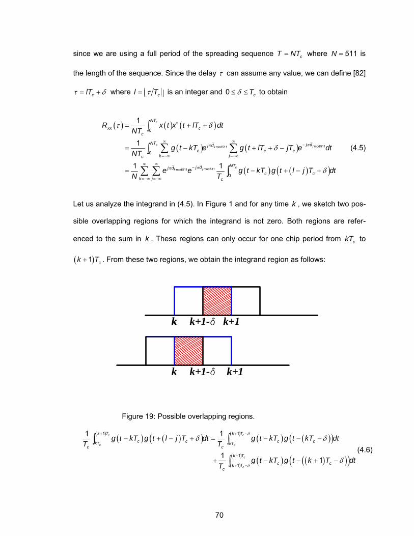
70

since we are using a full period of the spreading sequence cT NT= where 511N = is

the length of the sequence. Since the delay τ can assume any value, we can define [82]

clTτ δ= + where cl Tτ= ⎢ ⎥⎣ ⎦ is an integer and 0 cTδ≤ ≤ to obtain

( ) ( ) ( )

( ) ( )

( ) ( )( )

mod511mod511

mod511mod511

0

0

0

1

1

1 1

c

c jk

cjk

NT

xx cc

NT j dj dc c c

k jc

NTj dj dc c

k j c

R x t x t lT dtNT

g t kT e g t lT jT e dtNT

e e g t kT g t l j T dtN T

ππ

ππ

τ δ

δ

δ

∗

∞ ∞−

=−∞ =−∞

∞ ∞−

=−∞ =−∞

= + +

= − + + −

= − + − +

∫

∑ ∑∫

∑ ∑ ∫

(4.5)

Let us analyze the integrand in (4.5). In Figure 1 and for any time k , we sketch two pos-

sible overlapping regions for which the integrand is not zero. Both regions are refer-

enced to the sum in k . These regions can only occur for one chip period from ckT to

( )1 ck T+ . From these two regions, we obtain the integrand region as follows:

k k+1-dk k+1

k k+1-d k+1

Figure 19: Possible overlapping regions.

( ) ( )( )( ) ( ) ( )( )( )

( ) ( )( )( )( )

( )

1 1

1

1

1 1

1 1

c c

c c

c

c

k T k T

c c c ckT kTc c

k T

c ck Tc

g t kT g t l j T dt g t kT g t kT dtT T

g t kT g t k T dtT

δ

δ

δ δ

δ

+ + −

+

+ −

− + − + = − − −

+ − − + −

∫ ∫

∫(4.6)

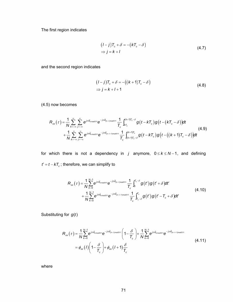
71

The first region indicates

( ) ( )c cl j T kT

j k lδ δ− + = − −

⇒ = + (4.7)

and the second region indicates

( ) ( )( )1

1c cl j T k T

j k l

δ δ− + = − + −

⇒ = + + (4.8)

(4.5) now becomes

( ) ( ) ( ) ( )( )( )

( ) ( ) ( )( )( )( )

( )

mod511mod511

1 mod511mod511

1

1

1

1 1

1 1 1

ck lk

c

ck lk

c

k Tj dj dxx c ckT

k j c

k Tj dj dc ck T

k j c

R e e g t kT g t kT dtN T

e e g t kT g t k T dtN T

δππ

ππ

δ

τ δ

δ

+

+ +

∞ ∞ + −−

=−∞ =−∞

∞ ∞ +−

+ −=−∞ =−∞

= − − −

+ − − + −

∑ ∑ ∫

∑ ∑ ∫(4.9)

for which there is not a dependency in j anymore, 0 1k N≤ ≤ − , and defining

ct t kT′ = − ; therefore, we can simplify to

( ) ( ) ( ) ( )

( ) ( ) ( )

mod511mod511

1 mod511mod511

1

00

1

0

1 1

1 1

ck lk

ck lk

c

N Tj dj dxx

k c

N Tj dj dcT

k c

R e e g t g t dtN T

e e g t g t T dtN T

δππ

ππ

δ

τ δ

δ

+

+ +

− −−

=

−−

−=

′ ′ ′= +

′ ′ ′+ − +

∑ ∫

∑ ∫ (4.10)

Substituting for ( )g t

( ) ( ) ( )

( ) ( )

mod511 1 mod511mod511 mod511

1 1

0 0

1 11

1 1

k l k lk k

N Nj d j dj d j dxx

k kc

xx xxc c

R e e e eN T N

l lT T

π ππ πδτ

δ δφ φ

+ + +− −

− −

= =

⎛ ⎞= − +⎜ ⎟

⎝ ⎠⎛ ⎞

= − + +⎜ ⎟⎝ ⎠

∑ ∑ (4.11)

where

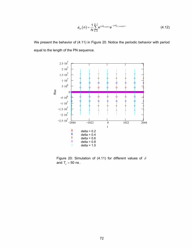
72

( ) ( )mod511mod511

1

0

1 k nk

N j dj dxx

kn e e

Nππφ +

−−

=

= ∑ (4.12)

We present the behavior of (4.11) in Figure 20. Notice the periodic behavior with period

equal to the length of the PN sequence.

2044 1022 0 1022 20442.5 .107

2 .1071.5 .107

1 .1075 .106

0

5 .1061 .107

1.5 .1072 .107

2.5 .107

delta = 0.2delta = 0.4delta = 0.6delta = 0.8delta = 1.0

l

Rxx

Figure 20: Simulation of (4.11) for different values of δ and 50 nscT = .

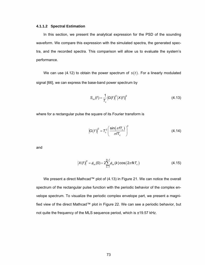
73

4.1.1.2 Spectral Estimation

In this section, we present the analytical expression for the PSD of the sounding

waveform. We compare this expression with the simulated spectra, the generated spec-

tra, and the recorded spectra. This comparison will allow us to evaluate the system’s

performance.

We can use (4.12) to obtain the power spectrum of ( )s t . For a linearly modulated

signal [66], we can express the base-band power spectrum by

2 21( ) ( ) ( )xxc

S f G f X fT

= (4.13)

where for a rectangular pulse the square of its Fourier transform is

( ) ( ) 22 2 sin c

cc

fTG f T

fTπ

π⎛ ⎞

= ⎜ ⎟⎝ ⎠

(4.14)

and

( )1

2

1( ) (0) 2 ( )cos 2

N

xx xx ck

X f k fkTφ φ π−

=

= + ∑ (4.15)

We present a direct Mathcad™ plot of (4.13) in Figure 21. We can notice the overall

spectrum of the rectangular pulse function with the periodic behavior of the complex en-

velope spectrum. To visualize the periodic complex envelope part, we present a magni-

fied view of the direct Mathcad™ plot in Figure 22. We can see a periodic behavior, but

not quite the frequency of the MLS sequence period, which is ±19.57 kHz.

74

4 .107 3 .107 2 .107 1 .107 0 1 .107 2 .107 3 .107 4 .10780

75

70

65

60

55

50

45

40Power Spectra

Frequency, Hz

Mag

nitu

de, d

B

Figure 21: Direct plot of (4.13) for 100 nscT = .

1 .105 8 .104 6 .104 4 .104 2 .104 0 2 .104 4 .104 6 .104 8 .104 1 .10550

46

42

38

34

30Power Spectra

frequency, Hz

Mag

nitu

de, d

B

Figure 22: Detailed view of the center peak of direct plot of (4.13).

We proceed to present the results of the Simulink™ simulation shown in Figure 23.

In Figure 24, we start with non-averaged (or snapshot) response of the Spectrum

Scope3 (the system does not allow editing; therefore, we apologize for the small font).

We can see a great resemblance to the direct plot of Figure 21. To obtain a detailed

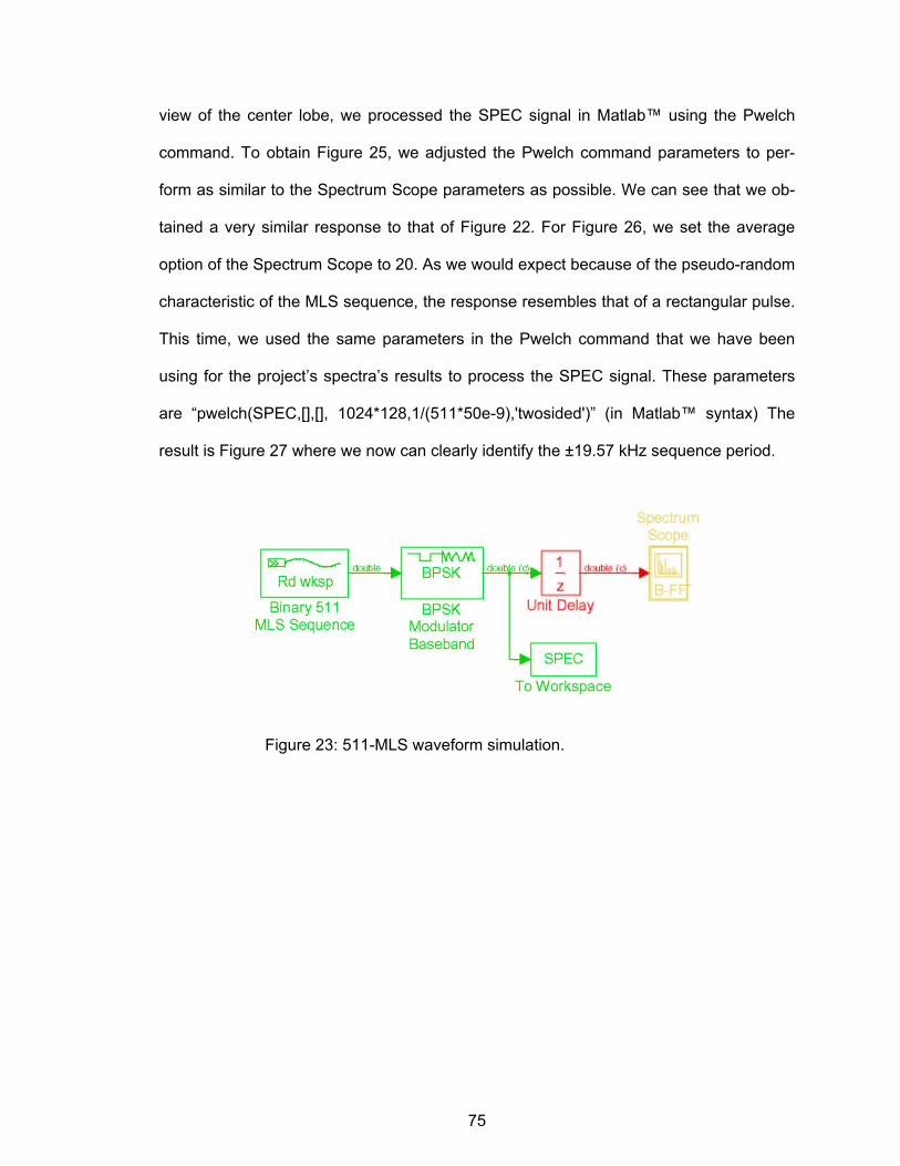
75

view of the center lobe, we processed the SPEC signal in Matlab™ using the Pwelch

command. To obtain Figure 25, we adjusted the Pwelch command parameters to per-

form as similar to the Spectrum Scope parameters as possible. We can see that we ob-

tained a very similar response to that of Figure 22. For Figure 26, we set the average

option of the Spectrum Scope to 20. As we would expect because of the pseudo-random

characteristic of the MLS sequence, the response resembles that of a rectangular pulse.

This time, we used the same parameters in the Pwelch command that we have been

using for the project’s spectra’s results to process the SPEC signal. These parameters

are “pwelch(SPEC,[],[], 1024*128,1/(511*50e-9),'twosided')” (in Matlab™ syntax) The

result is Figure 27 where we now can clearly identify the ±19.57 kHz sequence period.

Figure 23: 511-MLS waveform simulation.

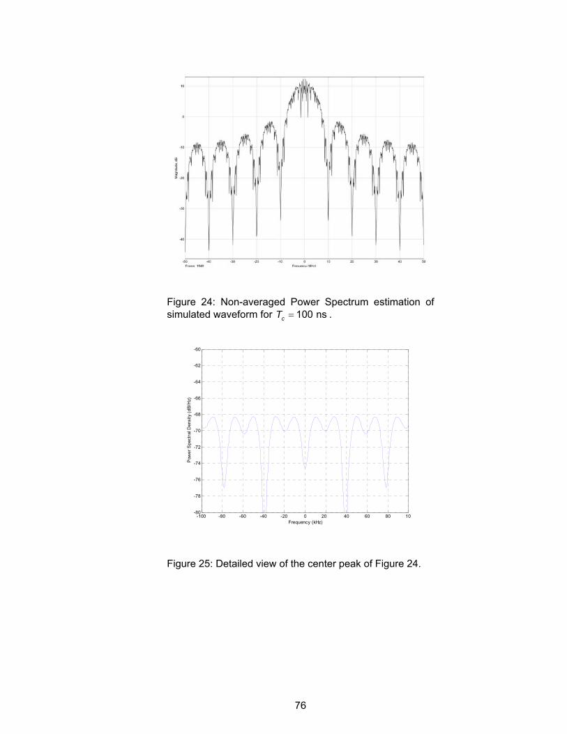
76

Figure 24: Non-averaged Power Spectrum estimation of simulated waveform for 100 nscT = .

-100 -80 -60 -40 -20 0 20 40 60 80 10 -80

-78

-76

-74

-72

-70

-68

-66

-64

-62

-60

Frequency (kHz)

Pow

er S

pect

ral D

ensi

ty (

dB/H

z)

Figure 25: Detailed view of the center peak of Figure 24.

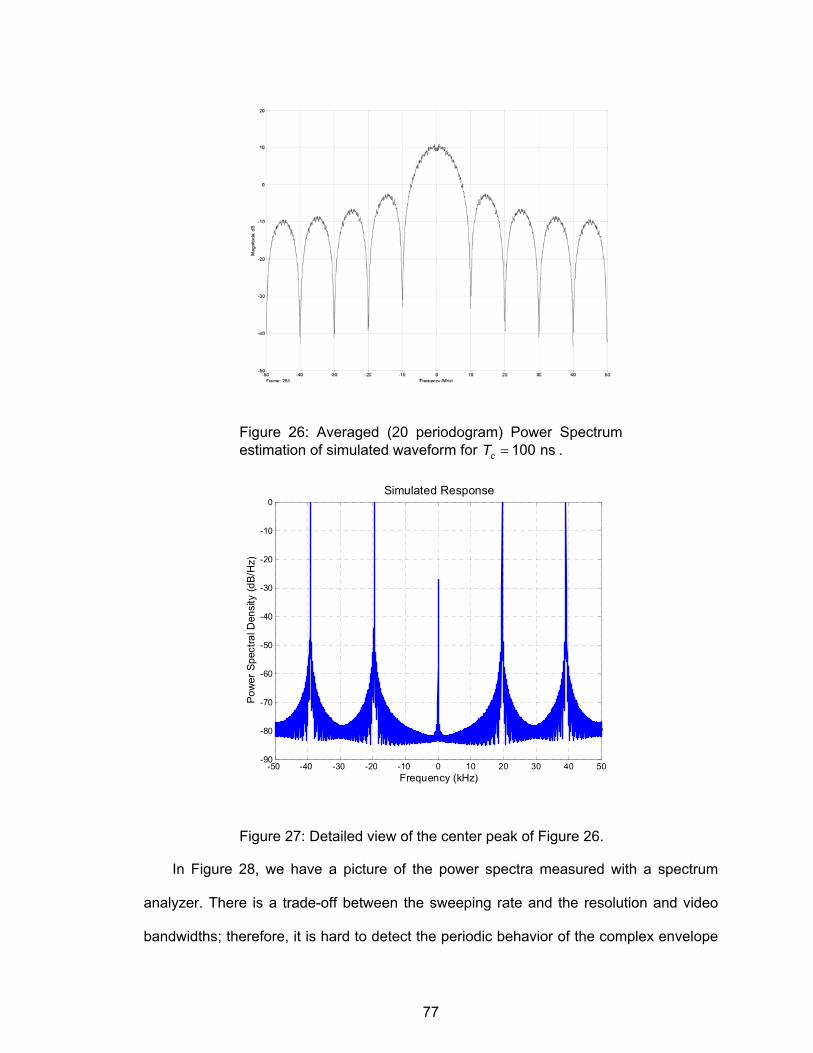
77

Figure 26: Averaged (20 periodogram) Power Spectrum estimation of simulated waveform for 100 nscT = .

-50 -40 -30 -20 -10 0 10 20 30 40 50-90

-80

-70

-60

-50

-40

-30

-20

-10

0

Pow

er S

pect

ral D

ensi

ty (d

B/H

z)

Frequency (kHz)

Simulated Response


In Figure 28, we have a picture of the power spectra measured with a spectrum

analyzer. There is a trade-off between the sweeping rate and the resolution and video

bandwidths; therefore, it is hard to detect the periodic behavior of the complex envelope

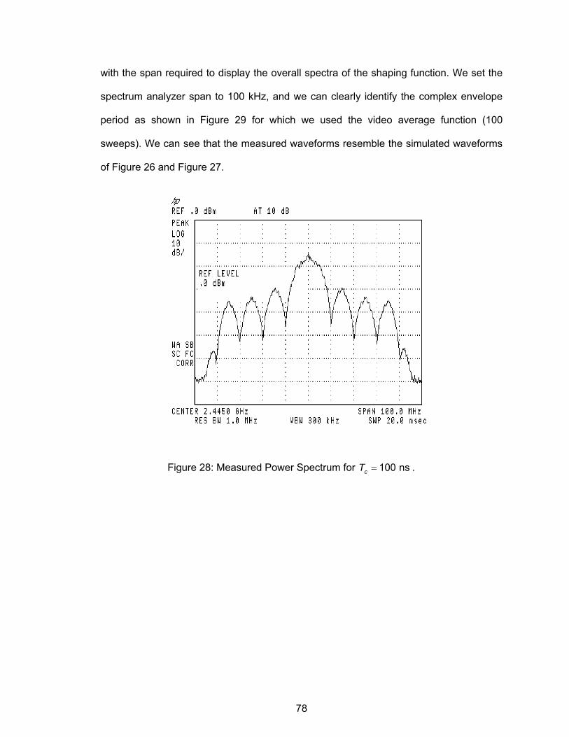
78

with the span required to display the overall spectra of the shaping function. We set the

spectrum analyzer span to 100 kHz, and we can clearly identify the complex envelope

period as shown in Figure 29 for which we used the video average function (100

sweeps). We can see that the measured waveforms resemble the simulated waveforms

of Figure 26 and Figure 27.

Figure 28: Measured Power Spectrum for 100 nscT = .

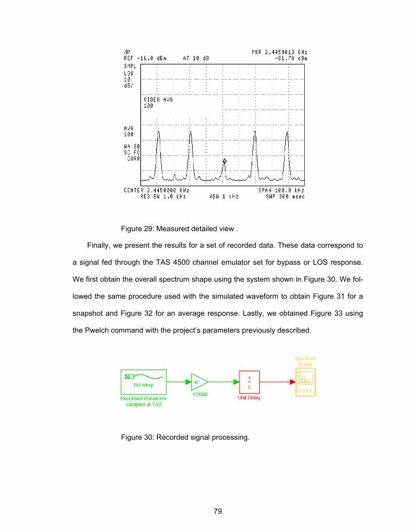
79

Figure 29: Measured detailed view .

Finally, we present the results for a set of recorded data. These data correspond to

a signal fed through the TAS 4500 channel emulator set for bypass or LOS response.

We first obtain the overall spectrum shape using the system shown in Figure 30. We fol-

lowed the same procedure used with the simulated waveform to obtain Figure 31 for a

snapshot and Figure 32 for an average response. Lastly, we obtained Figure 33 using

the Pwelch command with the project’s parameters previously described.

Figure 30: Recorded signal processing.

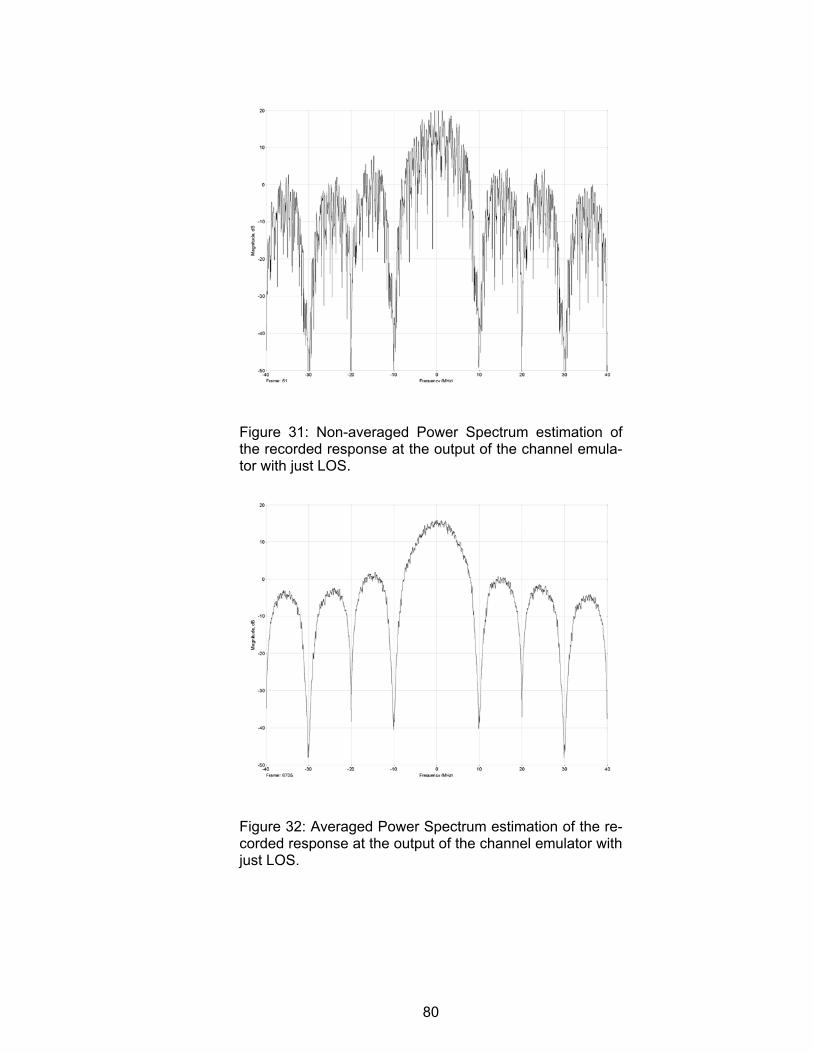
80

Figure 31: Non-averaged Power Spectrum estimation of the recorded response at the output of the channel emula-tor with just LOS.

Figure 32: Averaged Power Spectrum estimation of the re-corded response at the output of the channel emulator with just LOS.

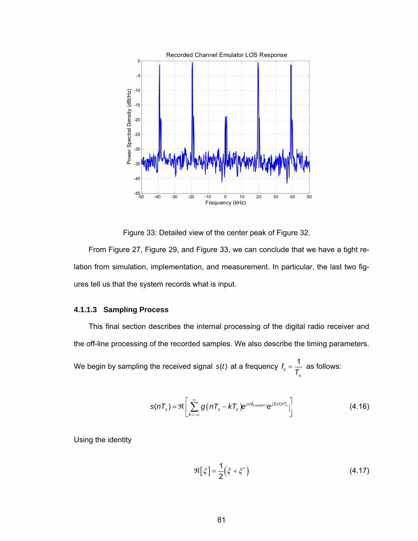
81

-50 -40 -30 -20 -10 0 10 20 30 40 50-45

-40

-35

-30

-25

-20

-15

-10

-5

0

Pow

er S

pect

ral D

ensi

ty (d

B/H

z)

Frequency (kHz)

Recorded Channel Emulator LOS Response


From Figure 27, Figure 29, and Figure 33, we can conclude that we have a tight re-

lation from simulation, implementation, and measurement. In particular, the last two fig-

ures tell us that the system records what is input.

4.1.1.3 Sampling Process

This final section describes the internal processing of the digital radio receiver and

the off-line processing of the recorded samples. We also describe the timing parameters.

We begin by sampling the received signal ( )s t at a frequency 1s

s

fT

= as follows:

( ) mod511 2( ) k I sj d j f nTs s c

ks nT g nT kT e eπ π

∞

=−∞

⎡ ⎤= ℜ −⎢ ⎥

⎣ ⎦∑ (4.16)

Using the identity

[ ] ( )12

ξ ξ ξ ∗ℜ = + (4.17)

82

we represent the sampled signal as

( ) ( ) ( )( )mod511 mod5112 21( )2

I s k I s kj f nT d j f nT ds s c

ks nT g nT kT e eπ π π π

∞+ − +

=−∞

= − +∑ (4.18)

We now proceed to down-convert to base-band

( ) ( )

( ) ( )( )mod511mod511

2

41 .2

I s

I s kk

j f nTs s

j f nT dj ds c

k

r nT s nT e

g nT kT e e

π

π ππ

−

∞− +

=−∞

=

= − +∑ (4.19)

The digital down-converter system in the Pentek digital radio receiver provides a

low-pass filter with a response close to 90 percent of half the Nyquist rate after decima-

tion. For example, a 80 MHzsf = corresponds to an 8x over-sampling for a 100 nscT =

or 8c

sTT = . If we band-limit the signal to its first 10 MHz null, we can decimate by four to

obtain a Nyquist frequency of 2N

c

fT

= giving two samples per baud. The corresponding

filter for these specifications is shown in Figure 34.

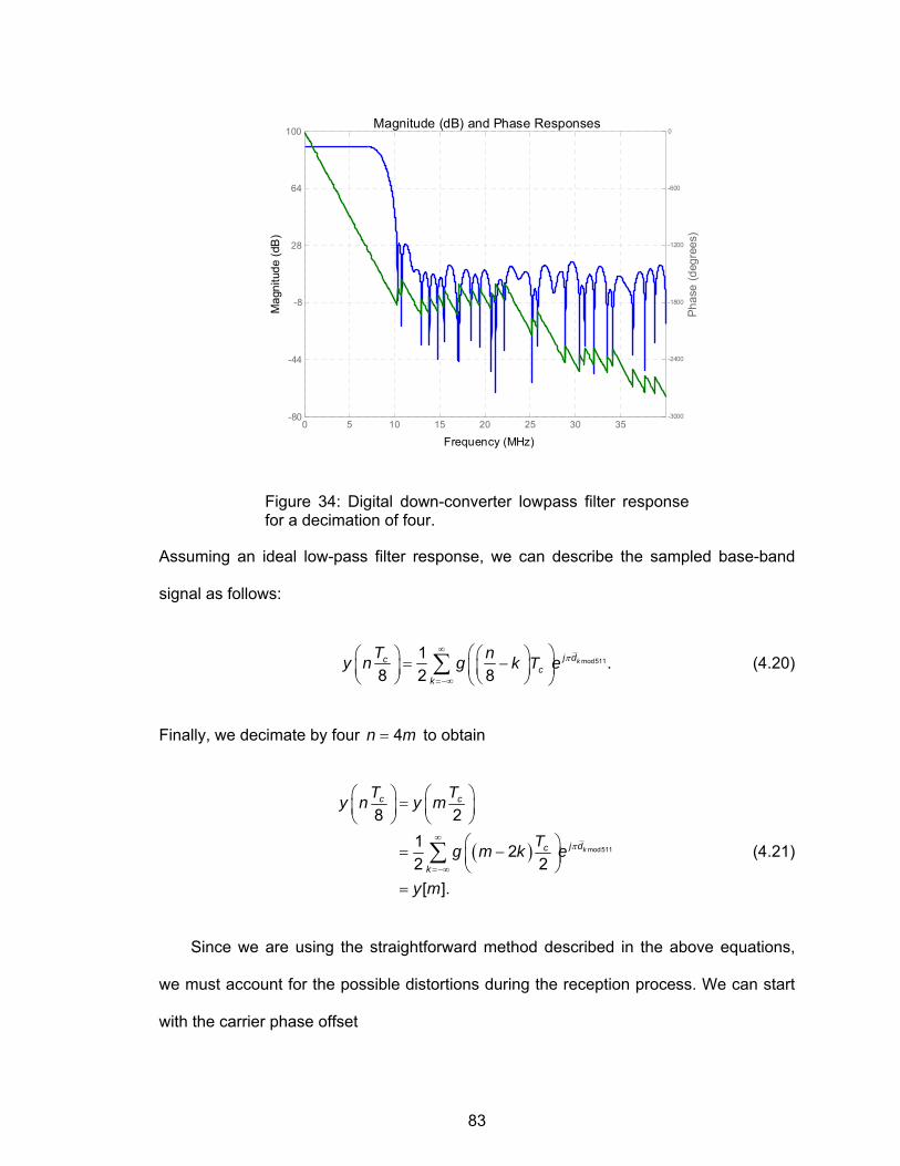
83

0 5 10 15 20 25 30 35-80

-44

-8

28

64

100

Frequency (MHz)

Mag

nitu

de (d

B)

Magnitude (dB) and Phase Responses

-3000

-2400

-1800

-1200

-600

0

Phas

e (d

egre

es)

Figure 34: Digital down-converter lowpass filter response for a decimation of four.

Assuming an ideal low-pass filter response, we can describe the sampled base-band

signal as follows:

mod5111 .

8 2 8kj dc

ck

T ny n g k T e π∞

=−∞

⎛ ⎞⎛ ⎞ ⎛ ⎞= −⎜ ⎟⎜ ⎟⎜ ⎟⎝ ⎠⎝ ⎠ ⎝ ⎠

∑ (4.20)

Finally, we decimate by four 4n m= to obtain

( ) mod511

8 21 22 2[ ].

k

c c

j dc

k

T Ty n y m

Tg m k e

y m

π∞

=−∞

⎛ ⎞ ⎛ ⎞=⎜ ⎟ ⎜ ⎟⎝ ⎠ ⎝ ⎠

⎛ ⎞= −⎜ ⎟⎝ ⎠

=

∑ (4.21)

Since we are using the straightforward method described in the above equations,

we must account for the possible distortions during the reception process. We can start

with the carrier phase offset

84

( ) mod511 2( ) ,k Ij d j f t jc

ks t g t kT e e eπ π θ

∞

=−∞

⎡ ⎤= ℜ −⎢ ⎥

⎣ ⎦∑ (4.22)

which produces a constellation rotation

( ) mod5111[ ] 2 .2 2

kj d jc

k

Ty m g m k e eπ θ∞

=−∞

⎛ ⎞= −⎜ ⎟⎝ ⎠

∑ (4.23)

We are mostly concerned with carrier frequency offset produced by the Doppler

characteristics of the channel. We can represent this carrier frequency offset as ( )Df t

and ignoring any other distortions, we have a received signal

( ) ( )

( ) ( )( )( )

mod511 22

mod511

( )

cos 2 ,

Dk I j f t tj d j f tc

k

c I D kk

s t g t kT e e e

g t kT f f t t d

ππ π

π π

∞

=−∞

∞

=−∞

⎡ ⎤= ℜ −⎢ ⎥

⎣ ⎦

= − + +

∑

∑ (4.24)

which produces a time dependant constellation rotation

( ) mod5112

21[ ] 2 .2 2

cD

k

Tj f mj dc

k

Ty m g m k e eπ

π⎛ ⎞∞ ⎜ ⎟⎝ ⎠

=−∞

⎛ ⎞= −⎜ ⎟⎝ ⎠

∑ (4.25)

The next step in the processing, which is done off-line in Matlab™, is the periodic

correlation. The operation is

[ ] [ ] [ ]1

0

N

jz k y k j a N j

−

=

= − −∑ (4.26)

where [ ]y k is the input real signal, N is the length of the MLS with coefficients [ ]a j .

Since this is a real operator, we first need to obtain the quadrature components of (4.25).

85

Considering that we are using a BPSK signal, mod511kj de π generates the real sequence

ja of 1± ’s, i.e., the PN sequence coefficients. The real and imaginary components are

[ ] ( )

[ ] ( )

mod511

mod511

1 2 cos 22 2 2

ˆ cos 22

1 2 sin 22 2 2

ˆ sin 2 .2

k

k

c cI D

k

cm D

c cQ D

k

cm D

T Ty m g m k a f m

Ta f m

T Ty m g m k a f m

Ta f m

π

π

π

π

∞

=−∞

∞

=−∞

⎛ ⎞⎛ ⎞ ⎛ ⎞= − ⎜ ⎟⎜ ⎟ ⎜ ⎟⎝ ⎠ ⎝ ⎠⎝ ⎠⎛ ⎞⎛ ⎞= ⎜ ⎟⎜ ⎟

⎝ ⎠⎝ ⎠⎛ ⎞⎛ ⎞ ⎛ ⎞= − ⎜ ⎟⎜ ⎟ ⎜ ⎟

⎝ ⎠ ⎝ ⎠⎝ ⎠⎛ ⎞⎛ ⎞= ⎜ ⎟⎜ ⎟

⎝ ⎠⎝ ⎠

∑

∑ (4.27)

From the sampling process just described, the main conclusion is that the recorded

samples will always have two samples per baud. As we will describe in Section 4.1.2.3,

this is one of the major restrictions of our system.

4.1.2 Post-Collection System Testing

This is one of the most important sections of this dissertation since it is here where

we assess the validity of the measurements.

4.1.2.1 Clock Synchronization

Since one of the main purposes of channel sounding is to measure small fade met-

rics, it is vital to have an adequate synchronization between the transmitting and receiv-

ing systems. Most communication systems must synchronize to a time or frequency

standard, i.e. an internal or external oscillator. Today’s technology provides four different

levels in frequency standards: cesium beam, hydrogen maser, rubidium, and quartz [83].

They are listed in descending order according to their accuracy and stability. The top

commercially available technology is the cesium beam standard. It is capable of provid-

ing an accuracy of a few parts in 1012 and a stability of a few parts in 1013/year. In many

86

channel sounding systems, it is common to use rubidium reference generators for syn-

chronization. Rubidium generators are much cheaper than the first two technologies, but

their stability reduces to approximately one part in 1011/month. The rubidium is generally

selected for applications in which the quartz crystal oscillator does not provide adequate

long-term stability, and cost and size considerations restrict the use of cesium beam

standards. The rubidium has excellent retrace characteristics (return to the frequency of

interest after a cold start) and warms up to its nominal frequency in a matter of minutes.

On the other hand, the quartz crystal oscillator has a number of qualities that make its

use as a reliable frequency standard desirable. It has mechanical stability and is rela-

tively immune to external environmental conditions. When connected into a closed loop

electric circuit in such a manner as to sustain oscillations and control the frequency of

oscillation, the quartz oscillator provides a convenient and reliable frequency source. To

improve the performance of the quartz oscillator, temperature compensation circuitry is

used to limit the variations in output frequency that result from variations in the operating

temperature. Crystal oscillators with such compensation are referred to as temperature

compensated crystal oscillators (TCXO). Another alternative to improve the stability is to

place the quartz in an oven controlled environment. This environment maintains a con-

stant temperature and provides shielding from the affects of line voltage.

For our measurement campaign, we used Agilent ESG series signal generators as

shown in Figure 18 where we display the complete system. For the receiver system, we

used the ESG E443xB series. This series has TCXO internal generators. For the trans-

mitter system, we used the ESG E4438C. This series has an improved internal oscilla-

tor. The specifications for the two signal generators are shown in Table 1, where we also

show the specifications for a commercially available rubidium generator for comparison.

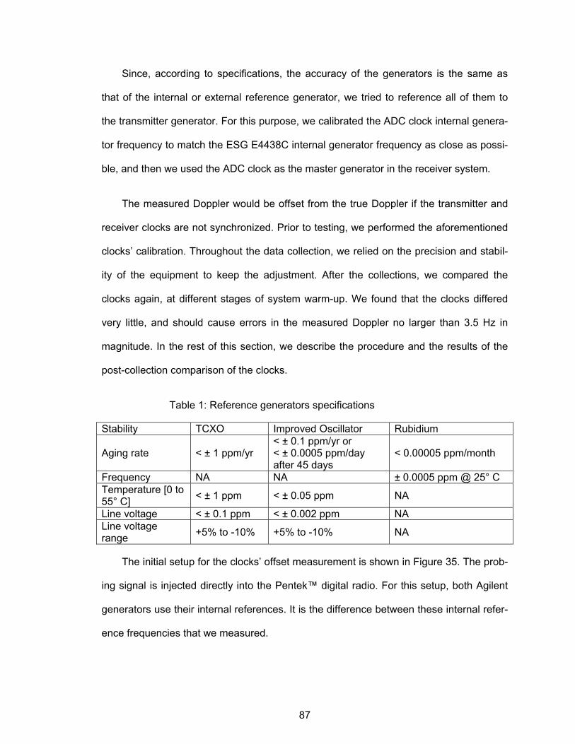
87

Since, according to specifications, the accuracy of the generators is the same as

that of the internal or external reference generator, we tried to reference all of them to

the transmitter generator. For this purpose, we calibrated the ADC clock internal genera-

tor frequency to match the ESG E4438C internal generator frequency as close as possi-

ble, and then we used the ADC clock as the master generator in the receiver system.

The measured Doppler would be offset from the true Doppler if the transmitter and

receiver clocks are not synchronized. Prior to testing, we performed the aforementioned

clocks’ calibration. Throughout the data collection, we relied on the precision and stabil-

ity of the equipment to keep the adjustment. After the collections, we compared the

clocks again, at different stages of system warm-up. We found that the clocks differed

very little, and should cause errors in the measured Doppler no larger than 3.5 Hz in

magnitude. In the rest of this section, we describe the procedure and the results of the

post-collection comparison of the clocks.

Table 1: Reference generators specifications

Stability TCXO Improved Oscillator Rubidium

Aging rate < ± 1 ppm/yr < ± 0.1 ppm/yr or < ± 0.0005 ppm/day after 45 days

< 0.00005 ppm/month

Frequency NA NA ± 0.0005 ppm @ 25° C Temperature [0 to 55° C] < ± 1 ppm < ± 0.05 ppm NA

Line voltage < ± 0.1 ppm < ± 0.002 ppm NA Line voltage range +5% to -10% +5% to -10% NA

The initial setup for the clocks’ offset measurement is shown in Figure 35. The prob-

ing signal is injected directly into the Pentek™ digital radio. For this setup, both Agilent

generators use their internal references. It is the difference between these internal refer-

ence frequencies that we measured.

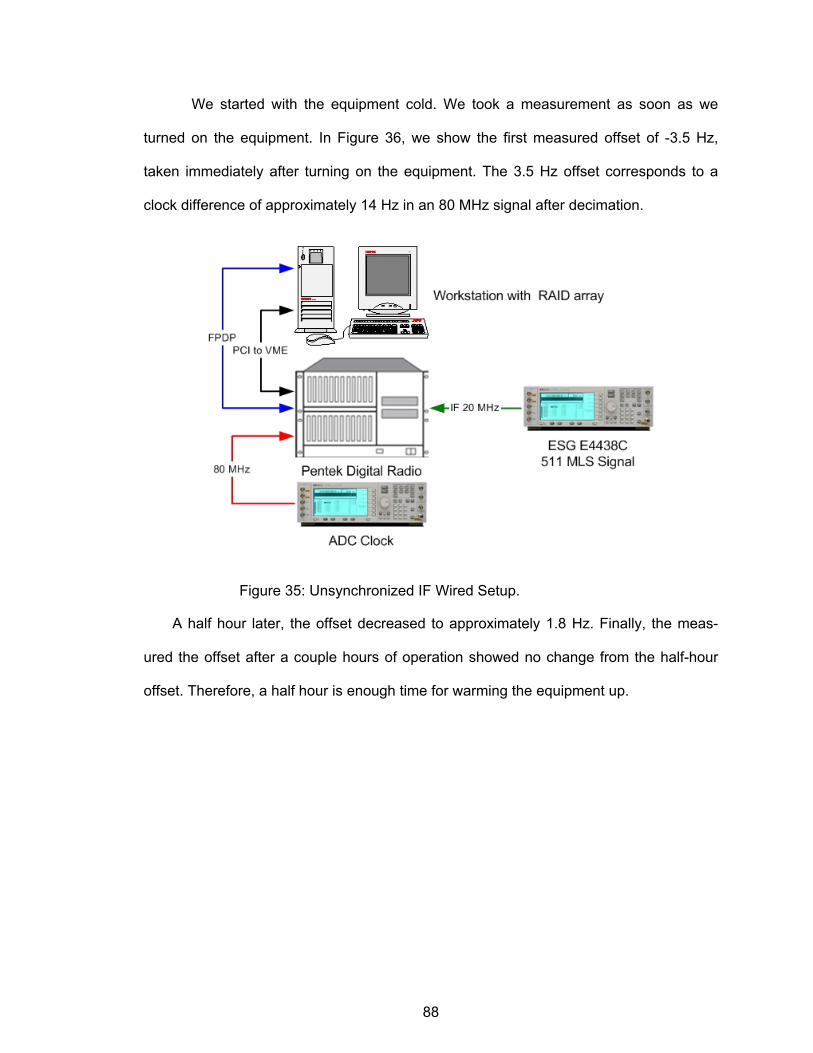
88

We started with the equipment cold. We took a measurement as soon as we

turned on the equipment. In Figure 36, we show the first measured offset of -3.5 Hz,

taken immediately after turning on the equipment. The 3.5 Hz offset corresponds to a

clock difference of approximately 14 Hz in an 80 MHz signal after decimation.

Figure 35: Unsynchronized IF Wired Setup.

A half hour later, the offset decreased to approximately 1.8 Hz. Finally, the meas-

ured the offset after a couple hours of operation showed no change from the half-hour

offset. Therefore, a half hour is enough time for warming the equipment up.

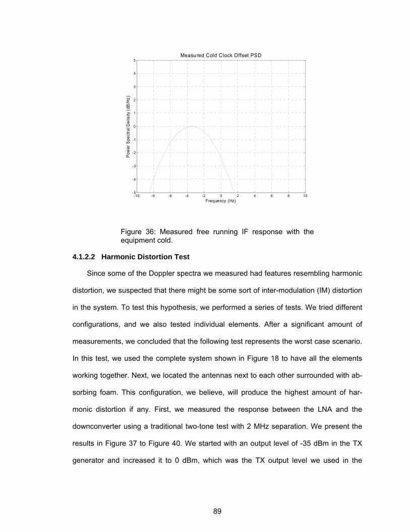
89

-10 -8 -6 -4 -2 0 2 4 6 8 10-5

-4

-3

-2

-1

0

1

2

3

4

5

Pow

er S

pect

ral D

ensi

ty (d

B/H

z)

Frequency (Hz)

Measured Cold Clock Offset PSD

Figure 36: Measured free running IF response with the equipment cold.

4.1.2.2 Harmonic Distortion Test

Since some of the Doppler spectra we measured had features resembling harmonic

distortion, we suspected that there might be some sort of inter-modulation (IM) distortion

in the system. To test this hypothesis, we performed a series of tests. We tried different

configurations, and we also tested individual elements. After a significant amount of

measurements, we concluded that the following test represents the worst case scenario.

In this test, we used the complete system shown in Figure 18 to have all the elements

working together. Next, we located the antennas next to each other surrounded with ab-

sorbing foam. This configuration, we believe, will produce the highest amount of har-

monic distortion if any. First, we measured the response between the LNA and the

downconverter using a traditional two-tone test with 2 MHz separation. We present the

results in Figure 37 to Figure 40. We started with an output level of -35 dBm in the TX

generator and increased it to 0 dBm, which was the TX output level we used in the

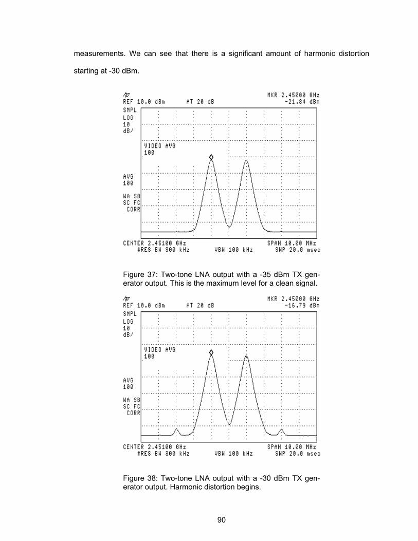
90

measurements. We can see that there is a significant amount of harmonic distortion

starting at -30 dBm.

Figure 37: Two-tone LNA output with a -35 dBm TX gen-erator output. This is the maximum level for a clean signal.

Figure 38: Two-tone LNA output with a -30 dBm TX gen-erator output. Harmonic distortion begins.

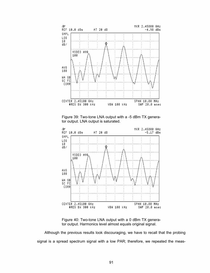
91

Figure 39: Two-tone LNA output with a -5 dBm TX genera-tor output. LNA output is saturated.

Figure 40: Two-tone LNA output with a 0 dBm TX genera-tor output. Harmonics level almost equals original signal.

Although the previous results look discouraging, we have to recall that the probing

signal is a spread spectrum signal with a low PAR; therefore, we repeated the meas-

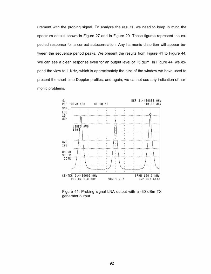
92

urement with the probing signal. To analyze the results, we need to keep in mind the

spectrum details shown in Figure 27 and in Figure 29. These figures represent the ex-

pected response for a correct autocorrelation. Any harmonic distortion will appear be-

tween the sequence period peaks. We present the results from Figure 41 to Figure 44.

We can see a clean response even for an output level of +5 dBm. In Figure 44, we ex-

pand the view to 1 KHz, which is approximately the size of the window we have used to

present the short-time Doppler profiles, and again, we cannot see any indication of har-

monic problems.

Figure 41: Probing signal LNA output with a -30 dBm TX generator output.

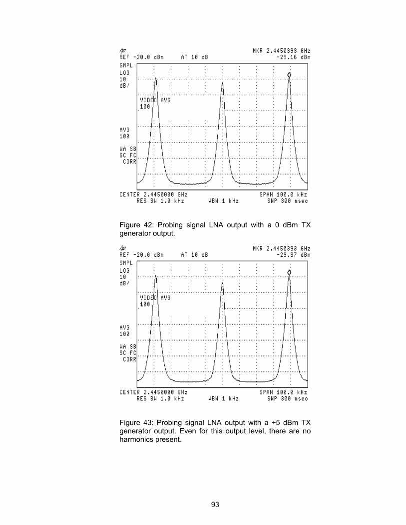
93

Figure 42: Probing signal LNA output with a 0 dBm TX generator output.

Figure 43: Probing signal LNA output with a +5 dBm TX generator output. Even for this output level, there are no harmonics present.

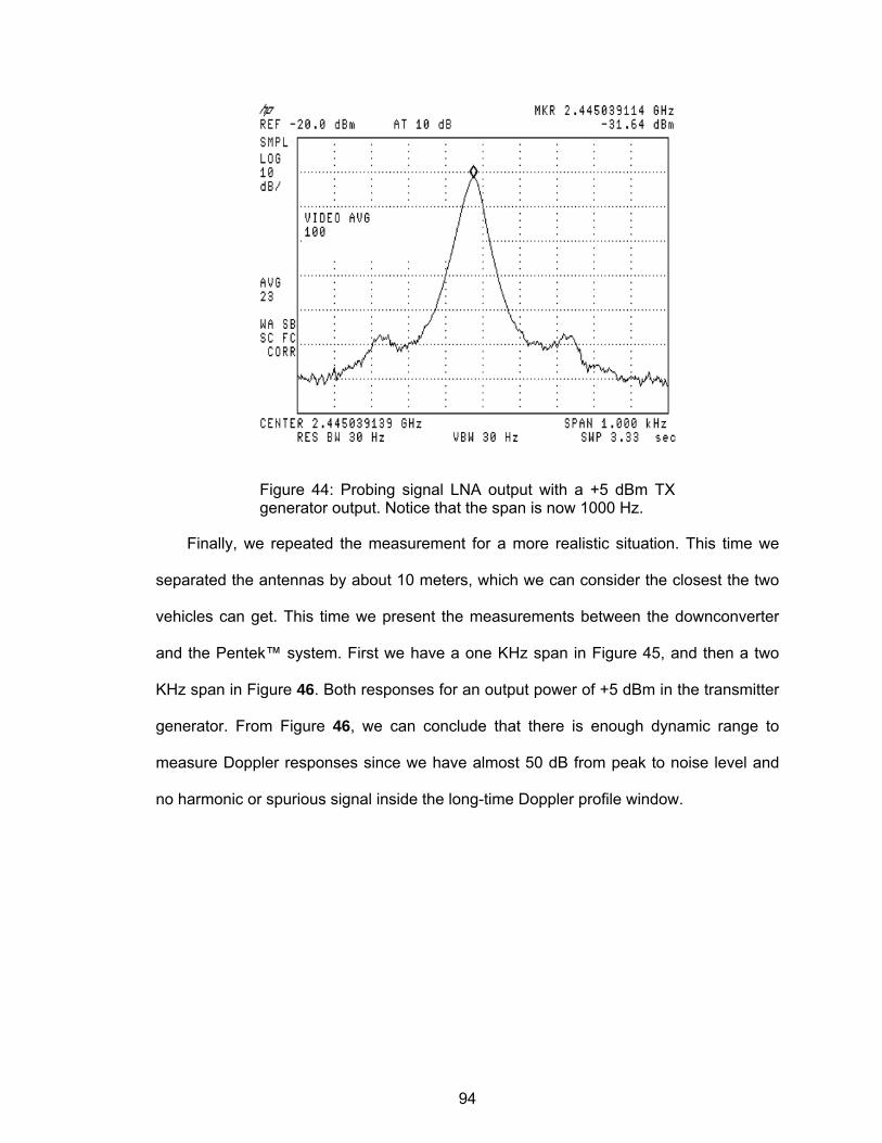
94

Figure 44: Probing signal LNA output with a +5 dBm TX generator output. Notice that the span is now 1000 Hz.

Finally, we repeated the measurement for a more realistic situation. This time we

separated the antennas by about 10 meters, which we can consider the closest the two

vehicles can get. This time we present the measurements between the downconverter

and the Pentek™ system. First we have a one KHz span in Figure 45, and then a two

KHz span in Figure 46. Both responses for an output power of +5 dBm in the transmitter

generator. From Figure 46, we can conclude that there is enough dynamic range to

measure Doppler responses since we have almost 50 dB from peak to noise level and

no harmonic or spurious signal inside the long-time Doppler profile window.

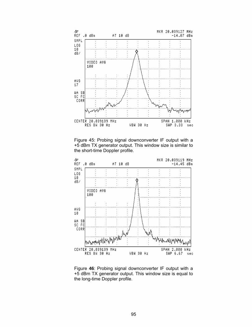
95

Figure 45: Probing signal downconverter IF output with a +5 dBm TX generator output. This window size is similar to the short-time Doppler profile.

Figure 46: Probing signal downconverter IF output with a +5 dBm TX generator output. This window size is equal to the long-time Doppler profile.

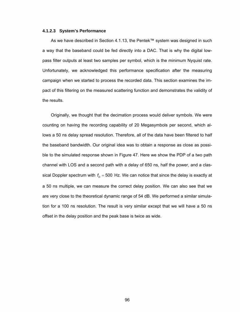
96

4.1.2.3 System’s Performance

As we have described in Section 4.1.13, the Pentek™ system was designed in such

a way that the baseband could be fed directly into a DAC. That is why the digital low-

pass filter outputs at least two samples per symbol, which is the minimum Nyquist rate.

Unfortunately, we acknowledged this performance specification after the measuring

campaign when we started to process the recorded data. This section examines the im-

pact of this filtering on the measured scattering function and demonstrates the validity of

the results.

Originally, we thought that the decimation process would deliver symbols. We were

counting on having the recording capability of 20 Megasymbols per second, which al-

lows a 50 ns delay spread resolution. Therefore, all of the data have been filtered to half

the baseband bandwidth. Our original idea was to obtain a response as close as possi-

ble to the simulated response shown in Figure 47. Here we show the PDP of a two path

channel with LOS and a second path with a delay of 650 ns, half the power, and a clas-

sical Doppler spectrum with 500Df = Hz. We can notice that since the delay is exactly at

a 50 ns multiple, we can measure the correct delay position. We can also see that we

are very close to the theoretical dynamic range of 54 dB. We performed a similar simula-

tion for a 100 ns resolution. The result is very similar except that we will have a 50 ns

offset in the delay position and the peak base is twice as wide.

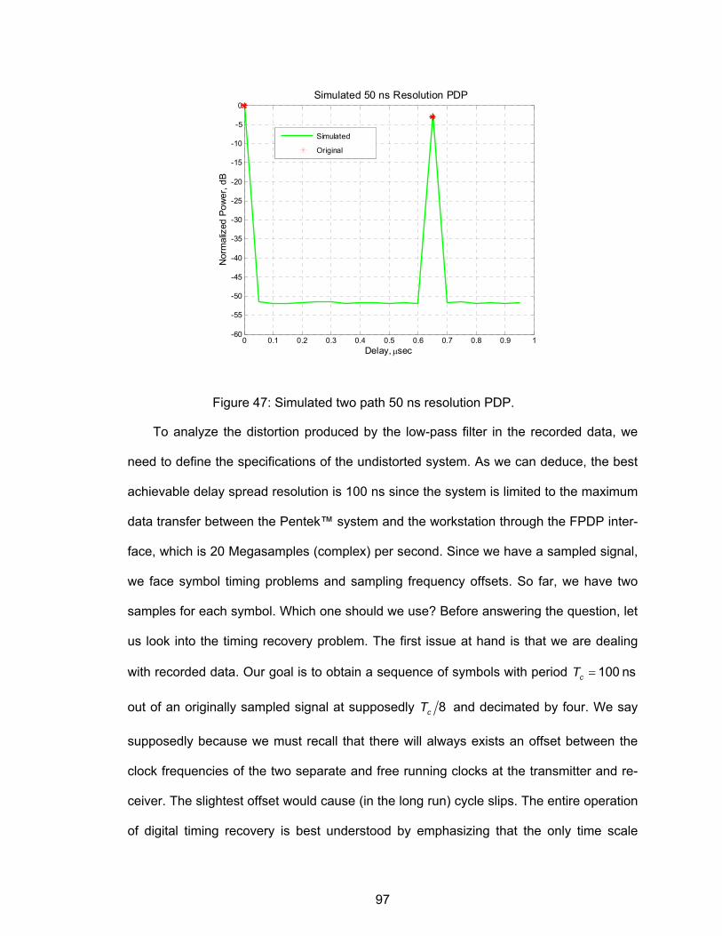
97

0 0.1 0.2 0.3 0.4 0.5 0.6 0.7 0.8 0.9 1-60

-55

-50

-45

-40

-35

-30

-25

-20

-15

-10

-5

0Simulated 50 ns Resolution PDP

Nor

mal

ized

Pow

er, d

B

Delay, μsec

Simulated

Original

Figure 47: Simulated two path 50 ns resolution PDP.

To analyze the distortion produced by the low-pass filter in the recorded data, we

need to define the specifications of the undistorted system. As we can deduce, the best

achievable delay spread resolution is 100 ns since the system is limited to the maximum

data transfer between the Pentek™ system and the workstation through the FPDP inter-

face, which is 20 Megasamples (complex) per second. Since we have a sampled signal,

we face symbol timing problems and sampling frequency offsets. So far, we have two

samples for each symbol. Which one should we use? Before answering the question, let

us look into the timing recovery problem. The first issue at hand is that we are dealing

with recorded data. Our goal is to obtain a sequence of symbols with period 100 nscT =

out of an originally sampled signal at supposedly 8cT and decimated by four. We say

supposedly because we must recall that there will always exists an offset between the

clock frequencies of the two separate and free running clocks at the transmitter and re-

ceiver. The slightest offset would cause (in the long run) cycle slips. The entire operation

of digital timing recovery is best understood by emphasizing that the only time scale

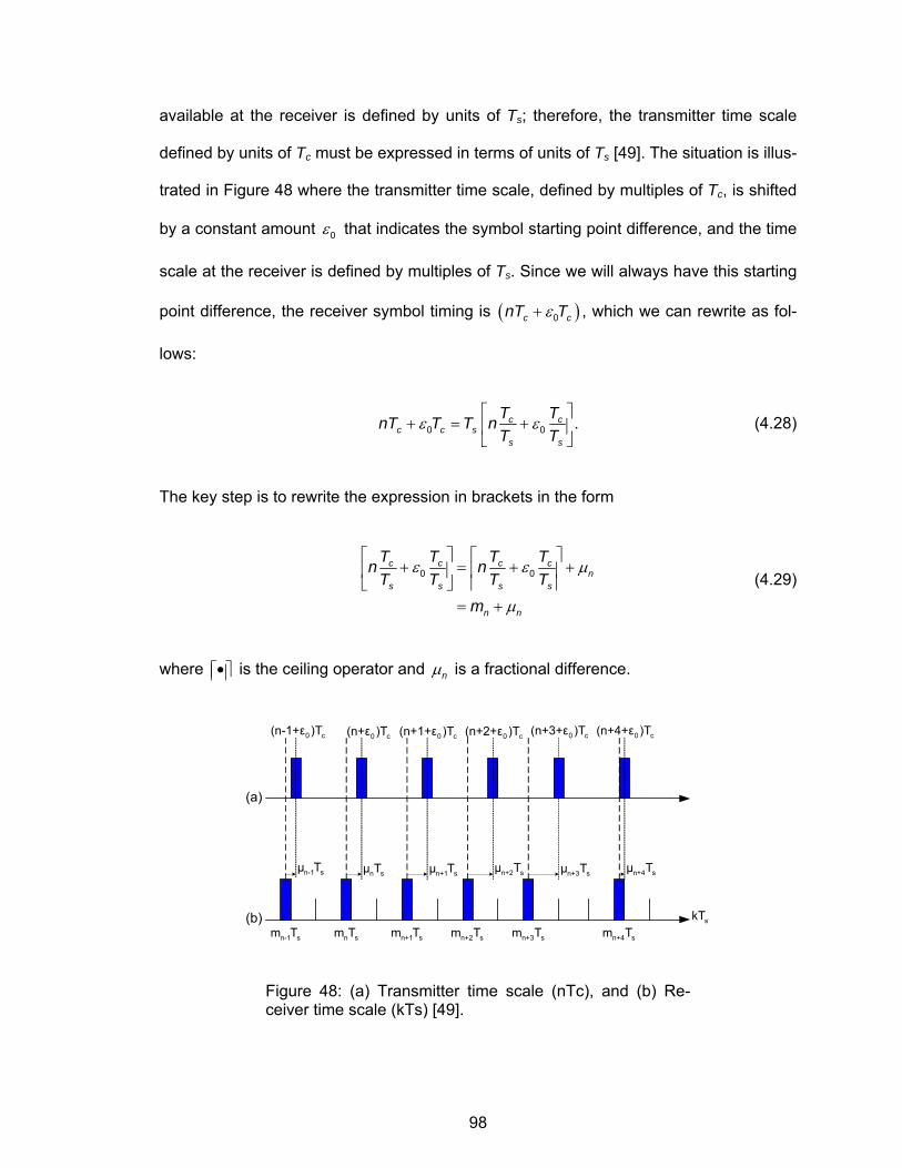
98

available at the receiver is defined by units of Ts; therefore, the transmitter time scale

defined by units of Tc must be expressed in terms of units of Ts [49]. The situation is illus-

trated in Figure 48 where the transmitter time scale, defined by multiples of Tc, is shifted

by a constant amount 0ε that indicates the symbol starting point difference, and the time

scale at the receiver is defined by multiples of Ts. Since we will always have this starting

point difference, the receiver symbol timing is ( )0c cnT Tε+ , which we can rewrite as fol-

lows:

0 0 .c cc c s

s s

T TnT T T nT T

ε ε⎡ ⎤

+ = +⎢ ⎥⎣ ⎦

(4.28)

The key step is to rewrite the expression in brackets in the form

0 0c c c c

ns s s s

n n

T T T Tn nT T T T

m

ε ε μ

μ

⎡ ⎤ ⎡ ⎤+ = + +⎢ ⎥ ⎢ ⎥

⎣ ⎦ ⎢ ⎥= +

(4.29)

where •⎡ ⎤⎢ ⎥ is the ceiling operator and nμ is a fractional difference.

n-1 sμ T n sμ T n+1 sμ T n+2 sμ T n+3 sμ T n+4 sμ T

0 c(n-1+ε )T 0 c(n+ε )T 0 c(n+1+ε )T 0 c(n+2+ε )T 0 c(n+3+ε )T 0 c(n+4+ε )T

(a)

(b) skT

n-1 sm T n sm T n+1 sm T n+2 sm T n+3 sm T n+4 sm T

Figure 48: (a) Transmitter time scale (nTc), and (b) Re-ceiver time scale (kTs) [49].

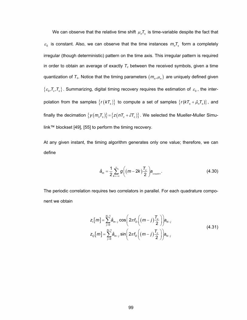
99

We can observe that the relative time shift n sTμ is time-variable despite the fact that

0ε is constant. Also, we can observe that the time instances n sm T form a completely

irregular (though deterministic) pattern on the time axis. This irregular pattern is required

in order to obtain an average of exactly Tc between the received symbols, given a time

quantization of Ts. Notice that the timing parameters ( ),n nm μ are uniquely defined given

{ }0, ,c sT Tε . Summarizing, digital timing recovery requires the estimation of 0ε , the inter-

polation from the samples ( ){ }sr kT to compute a set of samples { }( )ˆs n sr kT Tμ+ , and

finally the decimation ( ){ } ( ){ }ˆn s c cy m T z nT Tε= + . We selected the Mueller-Muller Simu-

link™ blockset [49], [55] to perform the timing recovery.

At any given instant, the timing algorithm generates only one value; therefore, we can

define

( )mod511

1ˆ 2 .2 2 k

cm

k

Ta g m k a∞

=−∞

⎛ ⎞= −⎜ ⎟⎝ ⎠

∑ (4.30)

The periodic correlation requires two correlators in parallel. For each quadrature compo-

nent we obtain

[ ] ( )

[ ] ( )

1

0

1

0

ˆ cos 22

ˆ sin 22

Nc

I m j D N jj

Nc

Q m j D N jj

Tz m a f m j a

Tz m a f m j a

π

π

−

− −=

−

− −=

⎛ ⎞⎛ ⎞= −⎜ ⎟⎜ ⎟⎝ ⎠⎝ ⎠

⎛ ⎞⎛ ⎞= −⎜ ⎟⎜ ⎟⎝ ⎠⎝ ⎠

∑

∑ (4.31)

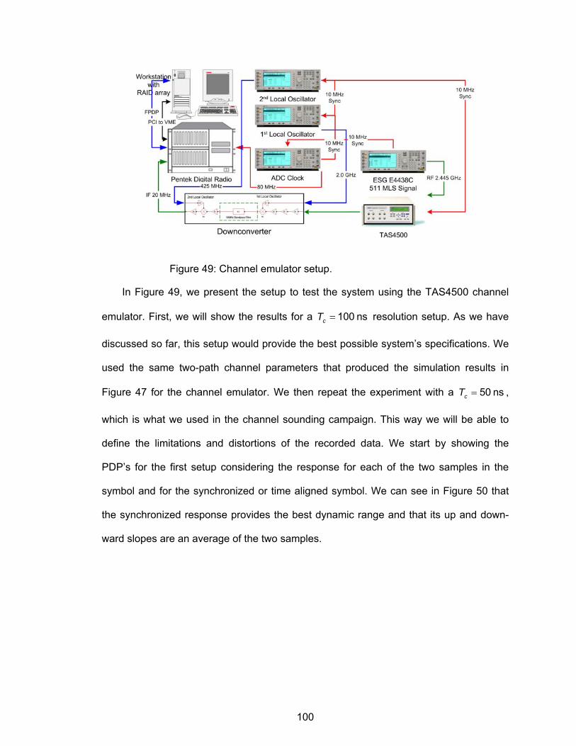
100

Figure 49: Channel emulator setup.

In Figure 49, we present the setup to test the system using the TAS4500 channel

emulator. First, we will show the results for a 100 nscT = resolution setup. As we have

discussed so far, this setup would provide the best possible system’s specifications. We

used the same two-path channel parameters that produced the simulation results in

Figure 47 for the channel emulator. We then repeat the experiment with a 50 nscT = ,

which is what we used in the channel sounding campaign. This way we will be able to

define the limitations and distortions of the recorded data. We start by showing the

PDP’s for the first setup considering the response for each of the two samples in the

symbol and for the synchronized or time aligned symbol. We can see in Figure 50 that

the synchronized response provides the best dynamic range and that its up and down-

ward slopes are an average of the two samples.

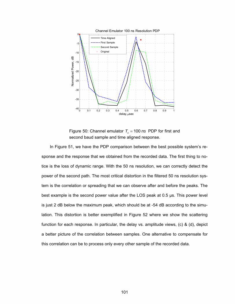
101

0 0.1 0.2 0.3 0.4 0.5 0.6 0.7 0.8 0.9 1-40

-35

-30

-25

-20

-15

-10

-5

0Channel Emulator 100 ns Resolution PDP

Nor

mal

ized

Pow

er, d

B

delay, μsec

Time Aligned

First Sample

Second Sample

Original

Figure 50: Channel emulator 100cT ns= PDP for first and second baud sample and time aligned response.

In Figure 51, we have the PDP comparison between the best possible system’s re-

sponse and the response that we obtained from the recorded data. The first thing to no-

tice is the loss of dynamic range. With the 50 ns resolution, we can correctly detect the

power of the second path. The most critical distortion in the filtered 50 ns resolution sys-

tem is the correlation or spreading that we can observe after and before the peaks. The

best example is the second power value after the LOS peak at 0.5 µs. This power level

is just 2 dB below the maximum peak, which should be at -54 dB according to the simu-

lation. This distortion is better exemplified in Figure 52 where we show the scattering

function for each response. In particular, the delay vs. amplitude views, (c) & (d), depict

a better picture of the correlation between samples. One alternative to compensate for

this correlation can be to process only every other sample of the recorded data.

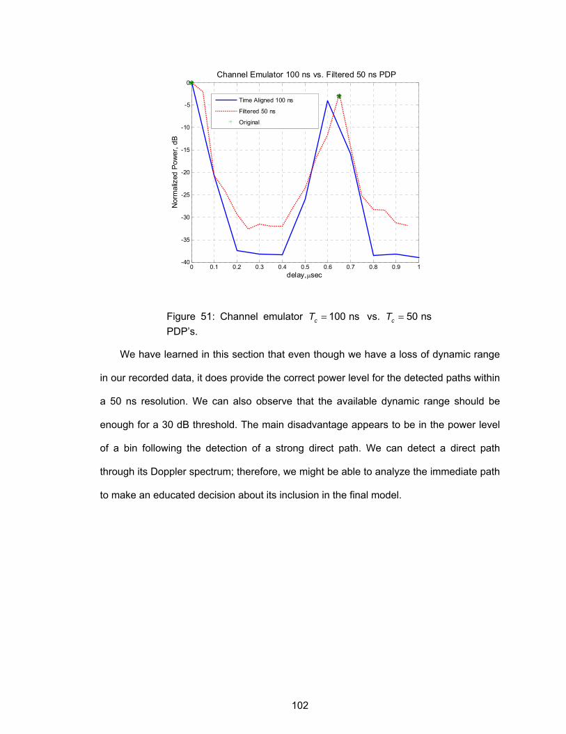
102

0 0.1 0.2 0.3 0.4 0.5 0.6 0.7 0.8 0.9 1-40

-35

-30

-25

-20

-15

-10

-5

0Channel Emulator 100 ns vs. Filtered 50 ns PDP

Nor

mal

ized

Pow

er, d

B

delay, μsec

Time Aligned 100 ns

Filtered 50 ns

Original

Figure 51: Channel emulator 100 nscT = vs. 50 nscT = PDP’s.

We have learned in this section that even though we have a loss of dynamic range

in our recorded data, it does provide the correct power level for the detected paths within

a 50 ns resolution. We can also observe that the available dynamic range should be

enough for a 30 dB threshold. The main disadvantage appears to be in the power level

of a bin following the detection of a strong direct path. We can detect a direct path

through its Doppler spectrum; therefore, we might be able to analyze the immediate path

to make an educated decision about its inclusion in the final model.

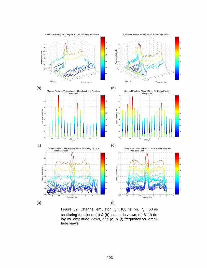
103

-.8-.6

-.4-.2

0 .2

.4 .6

.8

0

0.5

1

1.5

-70

-60

-50

-40

-30

-20

-10

0

Frequency, kHz

Channel Emulator Time Aligned 100 ns Scattering FunctionT

Delay, μs

Rel

ativ

e am

plitu

de, d

B

-60

-50

-40

-30

-20

-10

(a)

-.8-.6

-.4-.2

0 .2

.4 .6

.8

00.2

0.40.6

0.81

-70

-60

-50

-40

-30

-20

-10

0

Frequency, kHz

Channel Emulator Filtered 50 ns Scattering Function

Delay, μs

Rel

ativ

e am

plitu

de, d

B

-60

-50

-40

-30

-20

-10

(b)

0 0.2 0.4 0.6 0.8 1 1.2 1.4 1.6-70

-60

-50

-40

-30

-20

-10

0

Channel Emulator Time Aligned 100 ns Scattering FunctionDelay View

Delay, μs

Rel

ativ

e am

plitu

de, d

B

-60

-50

-40

-30

-20

-10

(c)

0 0.2 0.4 0.6 0.8 1-70

-60

-50

-40

-30

-20

-10

0

Channel Emulator Filtered 50 ns Scattering FunctionDelay View

Delay, μs

Rel

ativ

e am

plitu

de, d

B

-60

-50

-40

-30

-20

-10

(d)

-.8 -.6 -.4 -.2 0 .2 .4 .6 .8 -70

-60

-50

-40

-30

-20

-10

0

Channel Emulator Time Aligned 100 ns Scattering FunctionFrequency View

Frequency, kHz

Rel

ativ

e am

plitu

de, d

B

-60

-50

-40

-30

-20

-10

(e)

-.8 -.6 -.4 -.2 0 .2 .4 .6 .8 -70

-60

-50

-40

-30

-20

-10

0

Channel Emulator Filtered 50 ns Scattering FunctionFrequency View

Frequency, kHz

Rel

ativ

e am

plitu

de, d

B

-60

-50

-40

-30

-20

-10

(f)

Figure 52: Channel emulator 100 nscT = vs. 50 nscT = scattering functions: (a) & (b) Isometric views, (c) & (d) de-lay vs. amplitude views, and (e) & (f) frequency vs. ampli-tude views.

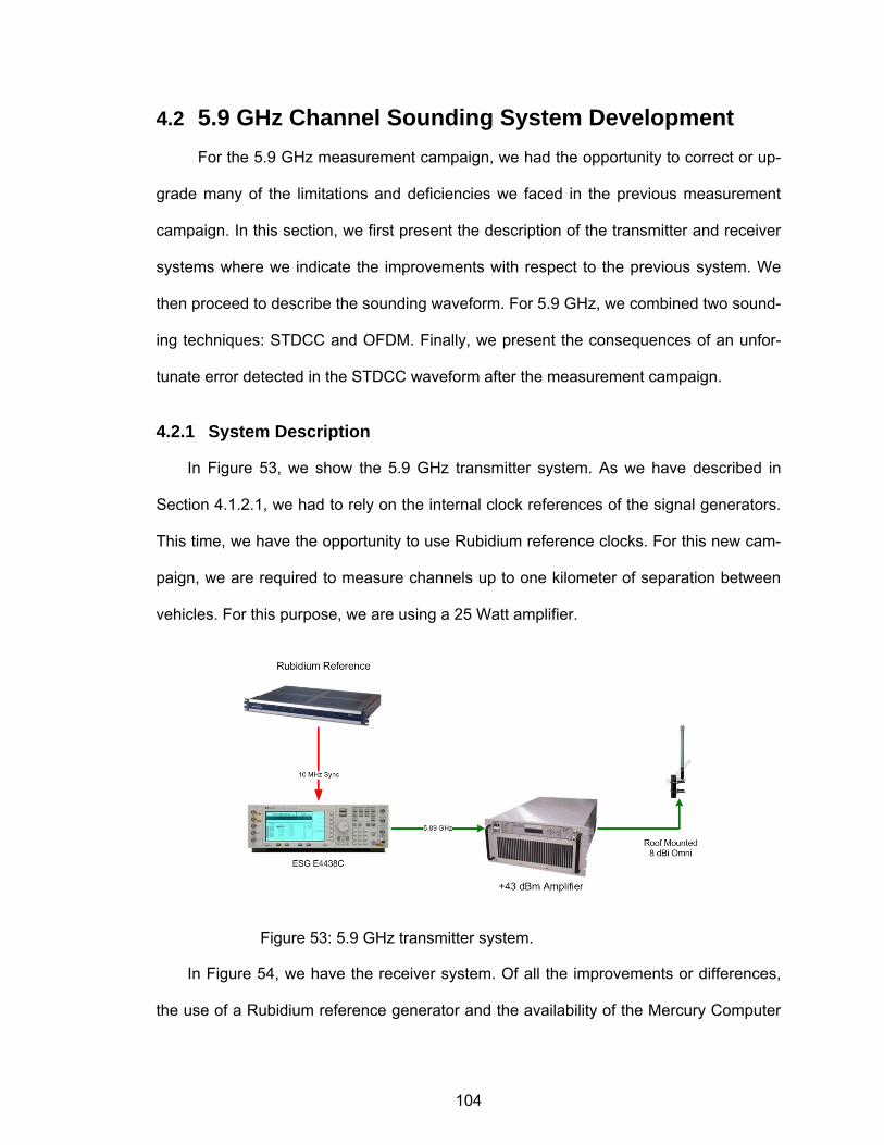
104

4.2 5.9 GHz Channel Sounding System Development For the 5.9 GHz measurement campaign, we had the opportunity to correct or up-

grade many of the limitations and deficiencies we faced in the previous measurement

campaign. In this section, we first present the description of the transmitter and receiver

systems where we indicate the improvements with respect to the previous system. We

then proceed to describe the sounding waveform. For 5.9 GHz, we combined two sound-

ing techniques: STDCC and OFDM. Finally, we present the consequences of an unfor-

tunate error detected in the STDCC waveform after the measurement campaign.

4.2.1 System Description

In Figure 53, we show the 5.9 GHz transmitter system. As we have described in

Section 4.1.2.1, we had to rely on the internal clock references of the signal generators.

This time, we have the opportunity to use Rubidium reference clocks. For this new cam-

paign, we are required to measure channels up to one kilometer of separation between

vehicles. For this purpose, we are using a 25 Watt amplifier.

Figure 53: 5.9 GHz transmitter system.

In Figure 54, we have the receiver system. Of all the improvements or differences,

the use of a Rubidium reference generator and the availability of the Mercury Computer

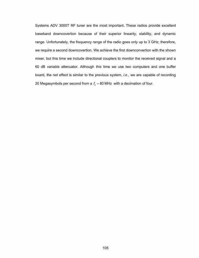
105

Systems ADV 3000T RF tuner are the most important. These radios provide excellent

baseband downcovertion because of their superior linearity, stability, and dynamic

range. Unfortunately, the frequency range of the radio goes only up to 3 GHz; therefore,

we require a second downcovertion. We achieve the first downconvertion with the shown

mixer, but this time we include directional couplers to monitor the received signal and a

60 dB variable attenuator. Although this time we use two computers and one buffer

board, the net effect is similar to the previous system, i.e., we are capable of recording

20 Megasymbols per second from a 80 MHzsf = with a decimation of four.

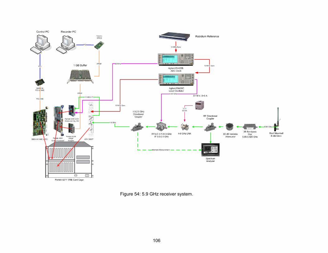
106

Figure 54: 5.9 GHz receiver system.

107

4.2.2 Sounding Waveform

As we described in Section 4.1.2.3, the maximum multipath resolution attainable

with an MLS sounding signal is 100 ns. We also mentioned in Section Error! Reference

source not found. that it is possible to double this maximum resolution using an OFDM

sounding waveform. For this campaign, we used a combined, MLS and OFDM, sound-

ing waveform. As we have indicated in previous sections, a 511 MLS sequence with a

100 ns chip period provides a Doppler measuring range of ±9.78 kHz. This is more than

enough since we are not required to measure Doppler shifts greater than ±2,100 Hz [6].

In other words, we can have a sequence length of up to 450 μs.

This time, the sounding waveform contains four sections. The first section is a 511

MLS sequence with a 100 ns chip period. The second and fourth sections are 320 zeros

with a 50 ns period. The third section is an OFDM signal with a 512 FFT size with a

guard band of size 128 for a total length of 640 samples with also a 50 ns period. There-

fore, the total length of the combined sequence is (511x2)+(320x2)+(512+128)=2,302 for

a time of 115.1 μs and a Doppler range of ±4,345 Hz.

In Figure 55 and Figure 56, we show the PDPs obtained when we tested our com-

bined signal through a channel emulator set for a three-tap static channel. The delays

were 0, 100, and 250 nanoseconds, and the power settings were 0, -4, and -7 dB re-

spectively. In particular, we can see the improved time resolution by comparing their re-

sponses at 250 ns.

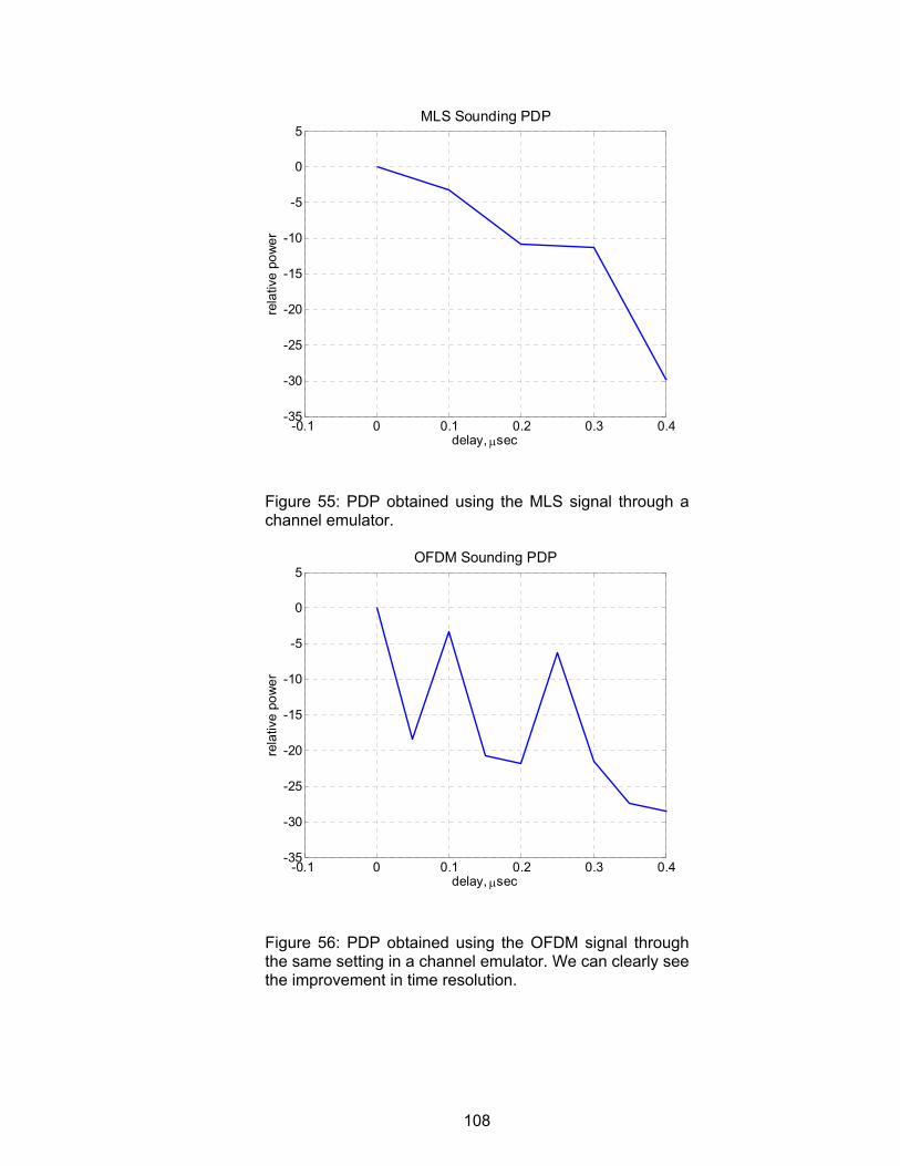
108

-0.1 0 0.1 0.2 0.3 0.4-35

-30

-25

-20

-15

-10

-5

0

5MLS Sounding PDP

rela

tive

pow

er

delay, μsec

Figure 55: PDP obtained using the MLS signal through a channel emulator.

-0.1 0 0.1 0.2 0.3 0.4-35

-30

-25

-20

-15

-10

-5

0

5OFDM Sounding PDP

rela

tive

pow

er

delay, μsec

Figure 56: PDP obtained using the OFDM signal through the same setting in a channel emulator. We can clearly see the improvement in time resolution.

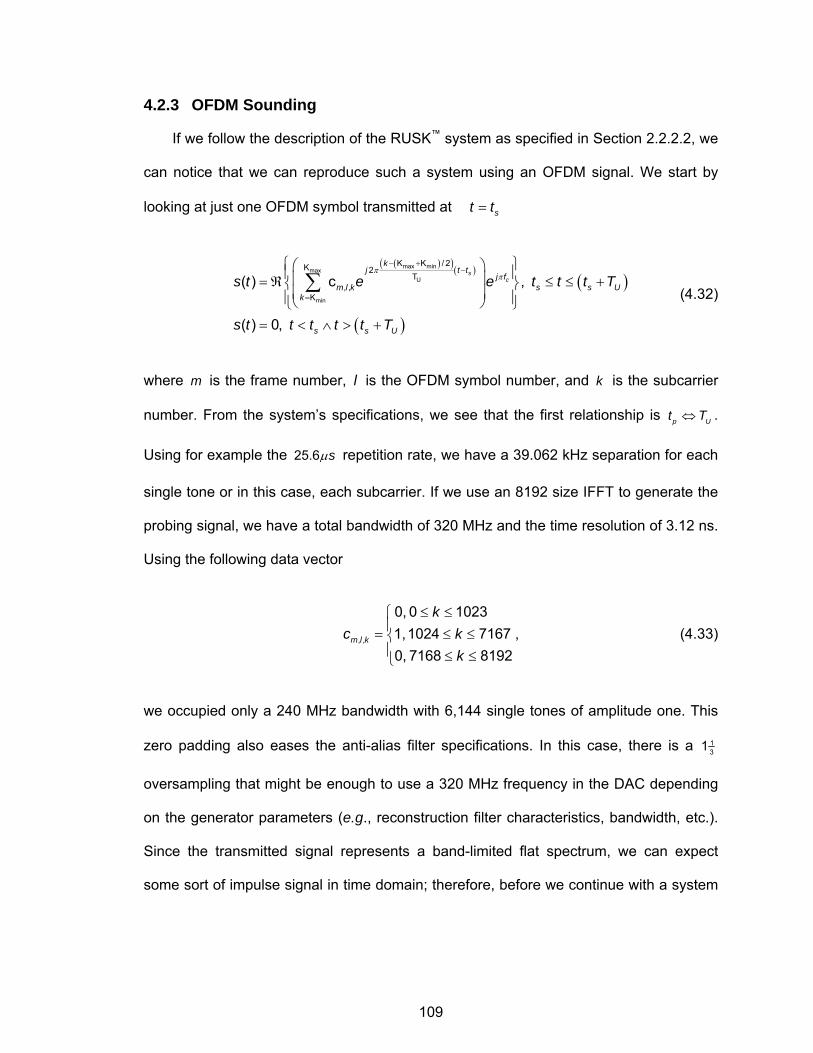
109

4.2.3 OFDM Sounding

If we follow the description of the RUSK™ system as specified in Section 2.2.2.2, we

can notice that we can reproduce such a system using an OFDM signal. We start by

looking at just one OFDM symbol transmitted at st t=

( )( )( )( )

( )

max minmax

U

min

K K / 2K 2T

, ,K

( ) c ,

( ) 0,

sc

kj t t

j fm l k s s U

k

s s U

s t e e t t t T

s t t t t t T

ππ

− +−

=

⎧ ⎫⎛ ⎞⎪ ⎪⎜ ⎟= ℜ ≤ ≤ +⎨ ⎬⎜ ⎟⎪ ⎪⎝ ⎠⎩ ⎭

= < ∧ > +

∑ (4.32)

where m is the frame number, l is the OFDM symbol number, and k is the subcarrier

number. From the system’s specifications, we see that the first relationship is p Ut T⇔ .

Using for example the 25.6 sμ repetition rate, we have a 39.062 kHz separation for each

single tone or in this case, each subcarrier. If we use an 8192 size IFFT to generate the

probing signal, we have a total bandwidth of 320 MHz and the time resolution of 3.12 ns.

Using the following data vector

, ,

0, 0 10231,1024 7167 ,0, 7168 8192

m l k

kc k

k

≤ ≤⎧⎪= ≤ ≤⎨⎪ ≤ ≤⎩

(4.33)

we occupied only a 240 MHz bandwidth with 6,144 single tones of amplitude one. This

zero padding also eases the anti-alias filter specifications. In this case, there is a 131

oversampling that might be enough to use a 320 MHz frequency in the DAC depending

on the generator parameters (e.g., reconstruction filter characteristics, bandwidth, etc.).

Since the transmitted signal represents a band-limited flat spectrum, we can expect

some sort of impulse signal in time domain; therefore, before we continue with a system

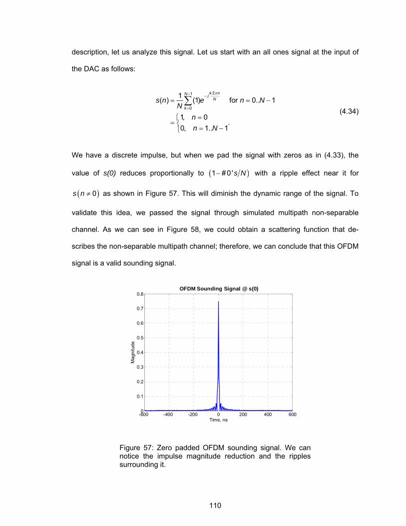
110

description, let us analyze this signal. Let us start with an all ones signal at the input of

the DAC as follows:

21

0

1( ) (1) for 0.. 1

1, 0.

0, 1.. 1

k nN jN

ks n e n N

Nnn N

π− −

=

= = −

=⎧= ⎨ = −⎩

∑ (4.34)

We have a discrete impulse, but when we pad the signal with zeros as in (4.33), the

value of s(0) reduces proportionally to ( )1 # 0's N− with a ripple effect near it for

( )0s n ≠ as shown in Figure 57. This will diminish the dynamic range of the signal. To

validate this idea, we passed the signal through simulated multipath non-separable

channel. As we can see in Figure 58, we could obtain a scattering function that de-

scribes the non-separable multipath channel; therefore, we can conclude that this OFDM

signal is a valid sounding signal.

-600 -400 -200 0 200 400 6000

0.1

0.2

0.3

0.4

0.5

0.6

0.7

0.8

Time, ns

Mag

nitu

de

OFDM Sounding Signal @ s(0)

Figure 57: Zero padded OFDM sounding signal. We can notice the impulse magnitude reduction and the ripples surrounding it.

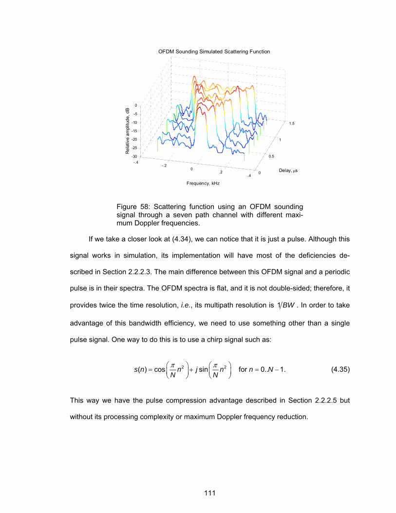
111

-.4 -.2

0 .2

.4 0

0.5

1

1.5

-30

-25

-20

-15

-10

-5

0

Delay, μs

Frequency, kHz

OFDM Sounding Simulated Scattering Function

Rel

ativ

e am

plitu

de, d

B

Figure 58: Scattering function using an OFDM sounding signal through a seven path channel with different maxi-mum Doppler frequencies.

If we take a closer look at (4.34), we can notice that it is just a pulse. Although this

signal works in simulation, its implementation will have most of the deficiencies de-

scribed in Section 2.2.2.3. The main difference between this OFDM signal and a periodic

pulse is in their spectra. The OFDM spectra is flat, and it is not double-sided; therefore, it

provides twice the time resolution, i.e., its multipath resolution is 1 BW . In order to take

advantage of this bandwidth efficiency, we need to use something other than a single

pulse signal. One way to do this is to use a chirp signal such as:

2 2( ) cos sin for 0.. 1.s n n j n n NN Nπ π⎛ ⎞ ⎛ ⎞= + = −⎜ ⎟ ⎜ ⎟

⎝ ⎠ ⎝ ⎠ (4.35)

This way we have the pulse compression advantage described in Section 2.2.2.5 but

without its processing complexity or maximum Doppler frequency reduction.

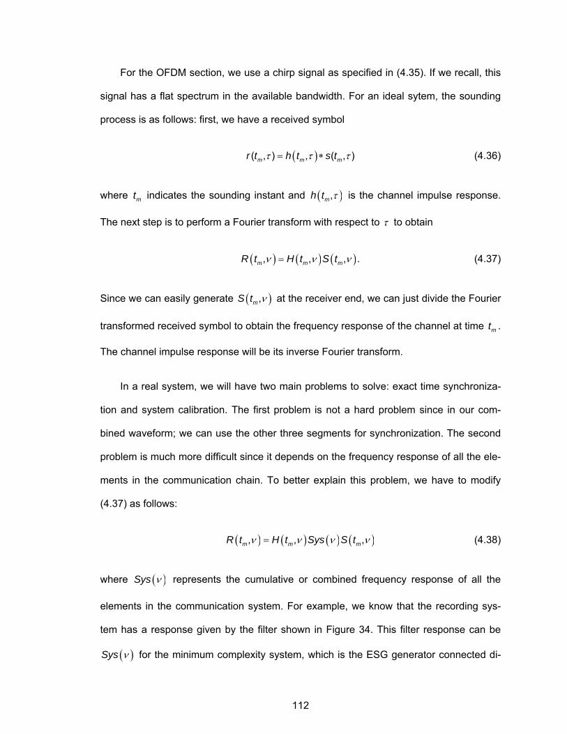
112

For the OFDM section, we use a chirp signal as specified in (4.35). If we recall, this

signal has a flat spectrum in the available bandwidth. For an ideal sytem, the sounding

process is as follows: first, we have a received symbol

( )( , ) , ( , )m m mr t h t s tτ τ τ= ∗ (4.36)

where mt indicates the sounding instant and ( ),mh t τ is the channel impulse response.

The next step is to perform a Fourier transform with respect to τ to obtain

( ) ( ) ( ), , , .m m mR t H t S tν ν ν= (4.37)

Since we can easily generate ( ),mS t ν at the receiver end, we can just divide the Fourier

transformed received symbol to obtain the frequency response of the channel at time mt .

The channel impulse response will be its inverse Fourier transform.

In a real system, we will have two main problems to solve: exact time synchroniza-

tion and system calibration. The first problem is not a hard problem since in our com-

bined waveform; we can use the other three segments for synchronization. The second

problem is much more difficult since it depends on the frequency response of all the ele-

ments in the communication chain. To better explain this problem, we have to modify

(4.37) as follows:

( ) ( ) ( ) ( ), , ,m m mR t H t Sys S tν ν ν ν= (4.38)

where ( )Sys ν represents the cumulative or combined frequency response of all the

elements in the communication system. For example, we know that the recording sys-

tem has a response given by the filter shown in Figure 34. This filter response can be

( )Sys ν for the minimum complexity system, which is the ESG generator connected di-

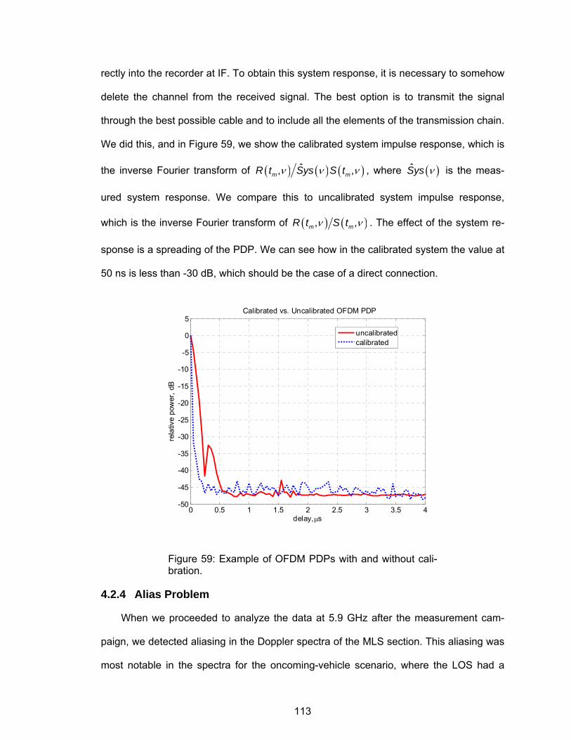
113

rectly into the recorder at IF. To obtain this system response, it is necessary to somehow

delete the channel from the received signal. The best option is to transmit the signal

through the best possible cable and to include all the elements of the transmission chain.

We did this, and in Figure 59, we show the calibrated system impulse response, which is

the inverse Fourier transform of ( ) ( ) ( )ˆ, ,m mR t Sys S tν ν ν , where ( )Sys ν is the meas-

ured system response. We compare this to uncalibrated system impulse response,

which is the inverse Fourier transform of ( ) ( ), ,m mR t S tν ν . The effect of the system re-

sponse is a spreading of the PDP. We can see how in the calibrated system the value at

50 ns is less than -30 dB, which should be the case of a direct connection.

0 0.5 1 1.5 2 2.5 3 3.5 4-50

-45

-40

-35

-30

-25

-20

-15

-10

-5

0

5

delay, μs

rela

tive

pow

er, d

B

Calibrated vs. Uncalibrated OFDM PDP

uncalibratedcalibrated

Figure 59: Example of OFDM PDPs with and without cali-bration.

4.2.4 Alias Problem

When we proceeded to analyze the data at 5.9 GHz after the measurement cam-

paign, we detected aliasing in the Doppler spectra of the MLS section. This aliasing was

most notable in the spectra for the oncoming-vehicle scenario, where the LOS had a

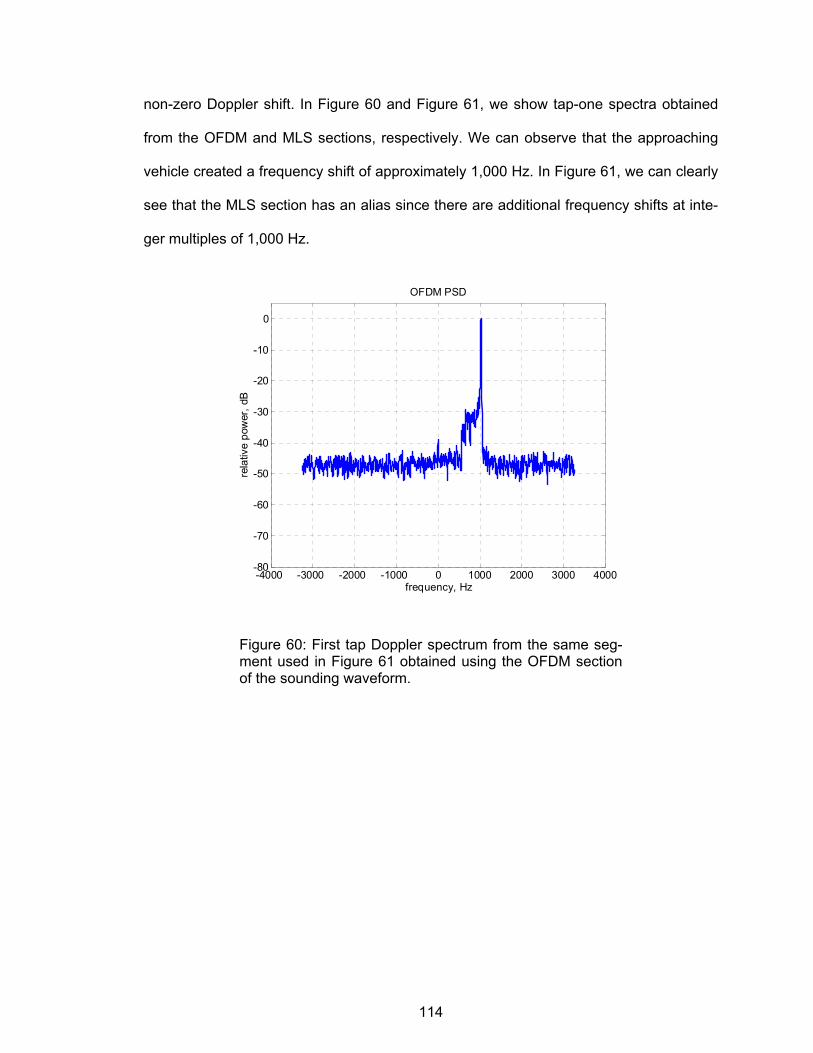
114

non-zero Doppler shift. In Figure 60 and Figure 61, we show tap-one spectra obtained

from the OFDM and MLS sections, respectively. We can observe that the approaching

vehicle created a frequency shift of approximately 1,000 Hz. In Figure 61, we can clearly

see that the MLS section has an alias since there are additional frequency shifts at inte-

ger multiples of 1,000 Hz.

-4000 -3000 -2000 -1000 0 1000 2000 3000 4000-80

-70

-60

-50

-40

-30

-20

-10

0

frequency, Hz

rela

tive

pow

er, d

B

OFDM PSD

Figure 60: First tap Doppler spectrum from the same seg-ment used in Figure 61 obtained using the OFDM section of the sounding waveform.

115

-4000 -3000 -2000 -1000 0 1000 2000 3000 4000-80

-70

-60

-50

-40

-30

-20

-10

0

frequency, Hz

rela

tive

pow

er, d

B

MLS PSD

Figure 61: First tap Doppler spectrum from an oncoming scenario segment obtained using the MLS section of the sounding waveform.

This happened because the IF of 10 MHz, while adequate for the OFDM section,

was not adequate for the MLS section. To see this, we first need to look at Figure 62,

where we show the measured spectrum of the OFDM section at the output of the ADV-

3000T. To show clearly that it only occupies 20 MHz, we used a 20 MHz IF. Therefore,

the optimum setting for the OFDM section was to use a 4x oversampling with the avail-

able 80 MHzsf = sampling frequency and a 10 MHz IF frequency. The ADV-3000T ra-

dios have a 40 MHz bandwidth passband filter at the baseband output. This is the main

anti-aliasing filter in the system. The combined waveform spectrum produced by the

ESG E4438C is shown in Figure 63. We can clearly observe the resulting sinc square

shape produced by the 100 ns rectangular pulse used for the MLS section. The MLS

section spectrum of the combined measured spectrum shown in Figure 63 is the same

as the one we showed in Figure 28 as expected. We could have avoided the problem if

we were able to filter the transmitter signal generator output with 20 MHz passband filter

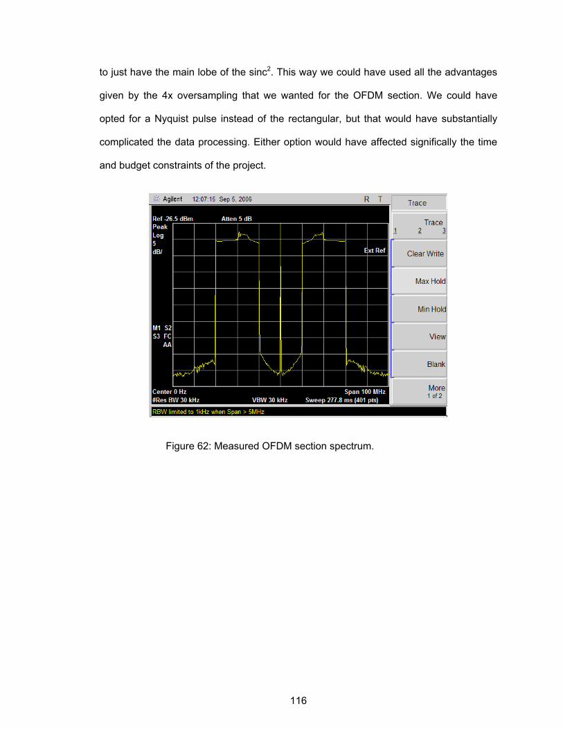
116

to just have the main lobe of the sinc2. This way we could have used all the advantages

given by the 4x oversampling that we wanted for the OFDM section. We could have

opted for a Nyquist pulse instead of the rectangular, but that would have substantially

complicated the data processing. Either option would have affected significally the time

and budget constraints of the project.

Figure 62: Measured OFDM section spectrum.

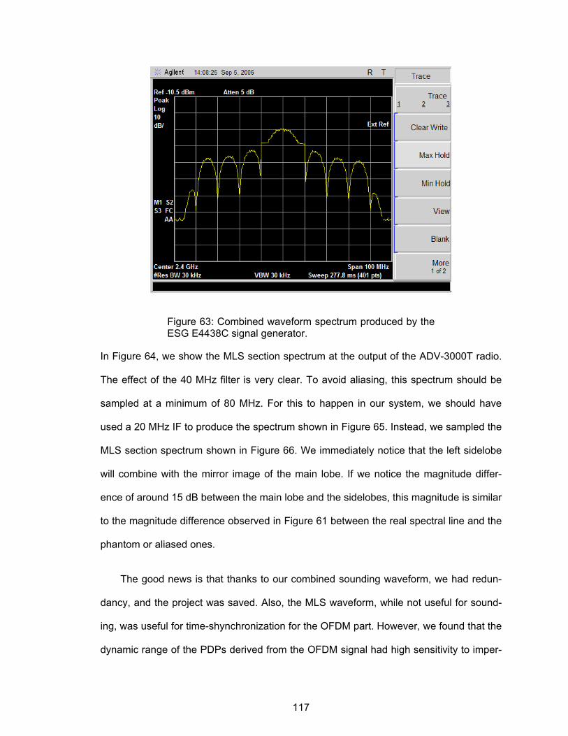
117

Figure 63: Combined waveform spectrum produced by the ESG E4438C signal generator.

In Figure 64, we show the MLS section spectrum at the output of the ADV-3000T radio.

The effect of the 40 MHz filter is very clear. To avoid aliasing, this spectrum should be

sampled at a minimum of 80 MHz. For this to happen in our system, we should have

used a 20 MHz IF to produce the spectrum shown in Figure 65. Instead, we sampled the

MLS section spectrum shown in Figure 66. We immediately notice that the left sidelobe

will combine with the mirror image of the main lobe. If we notice the magnitude differ-

ence of around 15 dB between the main lobe and the sidelobes, this magnitude is similar

to the magnitude difference observed in Figure 61 between the real spectral line and the

phantom or aliased ones.

The good news is that thanks to our combined sounding waveform, we had redun-

dancy, and the project was saved. Also, the MLS waveform, while not useful for sound-

ing, was useful for time-shynchronization for the OFDM part. However, we found that the

dynamic range of the PDPs derived from the OFDM signal had high sensitivity to imper-

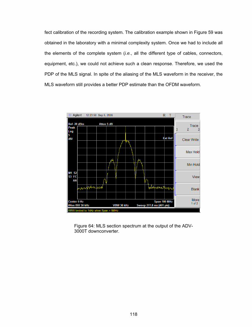
118

fect calibration of the recording system. The calibration example shown in Figure 59 was

obtained in the laboratory with a minimal complexity system. Once we had to include all

the elements of the complete system (i.e., all the different type of cables, connectors,

equipment, etc.), we could not achieve such a clean response. Therefore, we used the

PDP of the MLS signal. In spite of the aliasing of the MLS waveform in the receiver, the

MLS waveform still provides a better PDP estimate than the OFDM waveform.

Figure 64: MLS section spectrum at the output of the ADV-3000T downconverter.

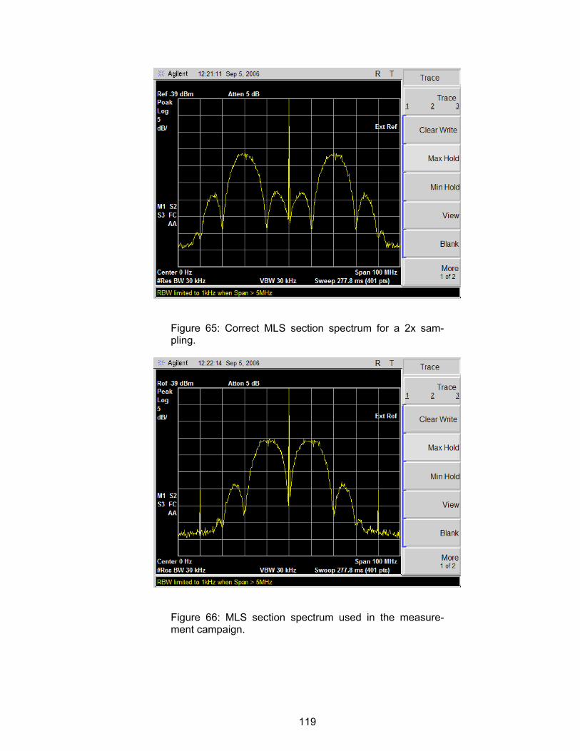
119

Figure 65: Correct MLS section spectrum for a 2x sam-pling.

Figure 66: MLS section spectrum used in the measure-ment campaign.

120

CHAPTER 5

MEASUREMENT CAMPAIGNS

In this chapter, we present an overview of the two measurement campaigns we per-

formed. The first campaign that we shall refer to as Phase One, started in June of 2003,

and concluded in December of 2004. The objective of Phase One was to identify the

worst case MTM channel. This campaign was performed at 2.4 GHz. The second cam-

paign or Phase Two was performed at 5.9 GHz during 2006. The objective of Phase

Two was to identify nominal channels at various specified ranges in specified environ-

ments.

5.1 Phase One: 2.4 GHz Measurement Campaign The most challenging environment for MTM communications is the doubly selective

channel that has large spreads in both delay and Doppler. We divided Phase One cam-

paign into two periods. In Period One, we measured only delay spreads. In Period Two,

we measured the doubly selective channel at only those sites found in Period One with

long delay spreads.

5.1.1 Period One: Finding Worst-Case Delay

This first period was simple and economical. The second period required a con-

siderable investment and logistics; therefore, it was very important to concentrate the

resources in sites that would provide adequate data to develop a “worst-case scenario”

model for future equipment testing. Using off-the-shelf 802.11b “sniffing” equipment, we

measured power delay profiles along several streets and freeways in the area surround-

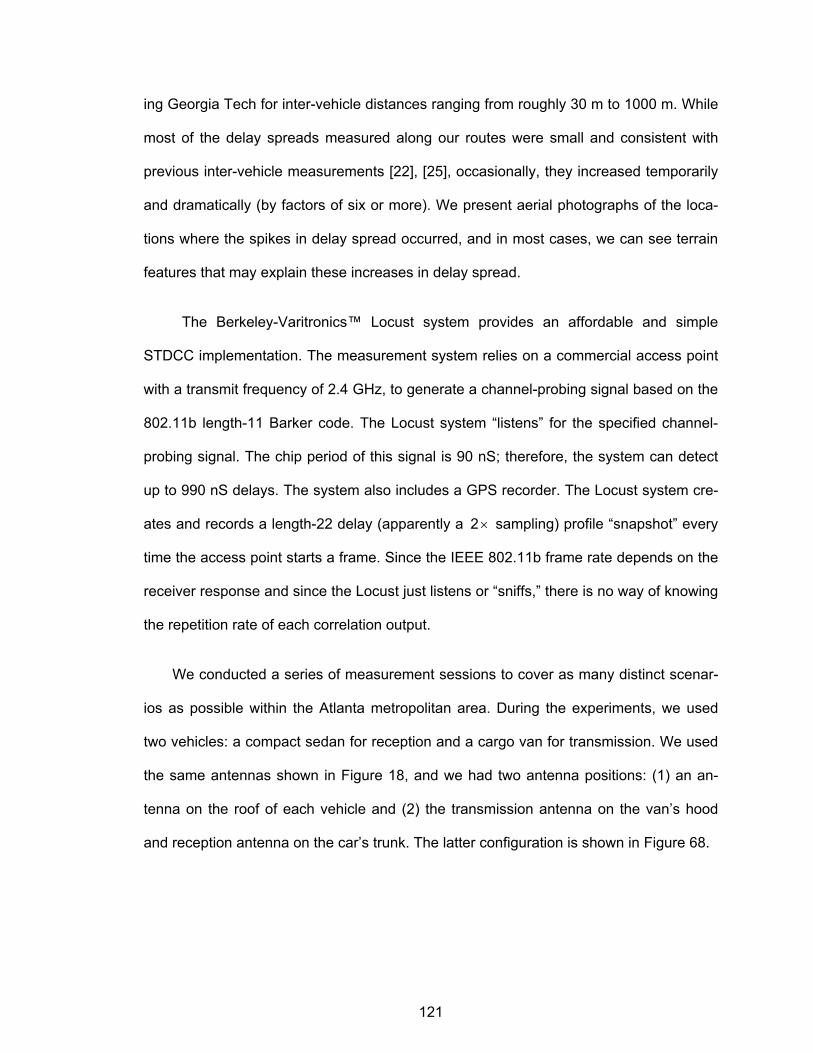
121

ing Georgia Tech for inter-vehicle distances ranging from roughly 30 m to 1000 m. While

most of the delay spreads measured along our routes were small and consistent with

previous inter-vehicle measurements [22], [25], occasionally, they increased temporarily

and dramatically (by factors of six or more). We present aerial photographs of the loca-

tions where the spikes in delay spread occurred, and in most cases, we can see terrain

features that may explain these increases in delay spread.

The Berkeley-Varitronics™ Locust system provides an affordable and simple

STDCC implementation. The measurement system relies on a commercial access point

with a transmit frequency of 2.4 GHz, to generate a channel-probing signal based on the

802.11b length-11 Barker code. The Locust system “listens” for the specified channel-

probing signal. The chip period of this signal is 90 nS; therefore, the system can detect

up to 990 nS delays. The system also includes a GPS recorder. The Locust system cre-

ates and records a length-22 delay (apparently a 2× sampling) profile “snapshot” every

time the access point starts a frame. Since the IEEE 802.11b frame rate depends on the

receiver response and since the Locust just listens or “sniffs,” there is no way of knowing

the repetition rate of each correlation output.

We conducted a series of measurement sessions to cover as many distinct scenar-

ios as possible within the Atlanta metropolitan area. During the experiments, we used

two vehicles: a compact sedan for reception and a cargo van for transmission. We used

the same antennas shown in Figure 18, and we had two antenna positions: (1) an an-

tenna on the roof of each vehicle and (2) the transmission antenna on the van’s hood

and reception antenna on the car’s trunk. The latter configuration is shown in Figure 68.

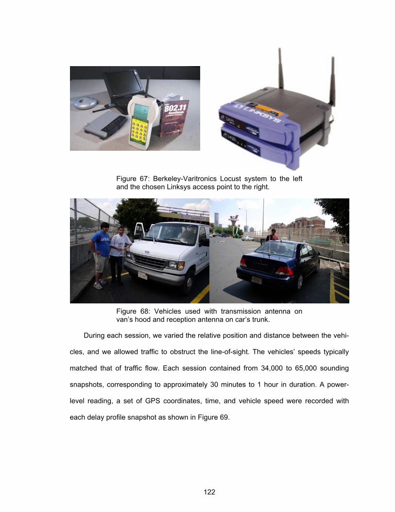
122

Figure 67: Berkeley-Varitronics Locust system to the left and the chosen Linksys access point to the right.

Figure 68: Vehicles used with transmission antenna on van’s hood and reception antenna on car’s trunk.

During each session, we varied the relative position and distance between the vehi-

cles, and we allowed traffic to obstruct the line-of-sight. The vehicles’ speeds typically

matched that of traffic flow. Each session contained from 34,000 to 65,000 sounding

snapshots, corresponding to approximately 30 minutes to 1 hour in duration. A power-

level reading, a set of GPS coordinates, time, and vehicle speed were recorded with

each delay profile snapshot as shown in Figure 69.

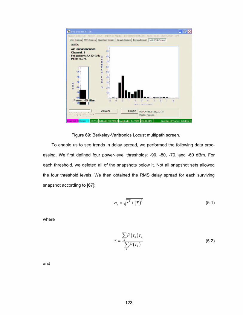
123

Figure 69: Berkeley-Varitronics Locust multipath screen.

To enable us to see trends in delay spread, we performed the following data proc-

essing. We first defined four power-level thresholds: -90, -80, -70, and -60 dBm. For

each threshold, we deleted all of the snapshots below it. Not all snapshot sets allowed

the four threshold levels. We then obtained the RMS delay spread for each surviving

snapshot according to [67]:

( )22τσ τ τ= + (5.1)

where

( )

( )k k

k

kk

P

P

τ ττ

τ=∑∑

(5.2)

and

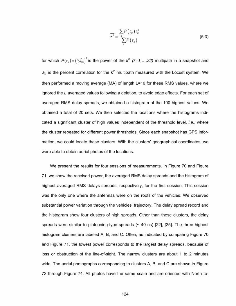
124

( )

( )

2

2k k

k

kk

P

P

τ ττ

τ=∑∑

(5.3)

for which ( )2100( ) ka

kP τ = is the power of the kth (k=1,…,22) multipath in a snapshot and

ka is the percent correlation for the kth multipath measured with the Locust system. We

then performed a moving average (MA) of length L=10 for these RMS values, where we

ignored the L averaged values following a deletion, to avoid edge effects. For each set of

averaged RMS delay spreads, we obtained a histogram of the 100 highest values. We

obtained a total of 20 sets. We then selected the locations where the histograms indi-

cated a significant cluster of high values independent of the threshold level, i.e., where

the cluster repeated for different power thresholds. Since each snapshot has GPS infor-

mation, we could locate these clusters. With the clusters’ geographical coordinates, we

were able to obtain aerial photos of the locations.

We present the results for four sessions of measurements. In Figure 70 and Figure

71, we show the received power, the averaged RMS delay spreads and the histogram of

highest averaged RMS delays spreads, respectively, for the first session. This session

was the only one where the antennas were on the roofs of the vehicles. We observed

substantial power variation through the vehicles’ trajectory. The delay spread record and

the histogram show four clusters of high spreads. Other than these clusters, the delay

spreads were similar to platooning-type spreads (~ 40 ns) [22], [25]. The three highest

histogram clusters are labeled A, B, and C. Often, as indicated by comparing Figure 70

and Figure 71, the lowest power corresponds to the largest delay spreads, because of

loss or obstruction of the line-of-sight. The narrow clusters are about 1 to 2 minutes

wide. The aerial photographs corresponding to clusters A, B, and C are shown in Figure

72 through Figure 74. All photos have the same scale and are oriented with North to-

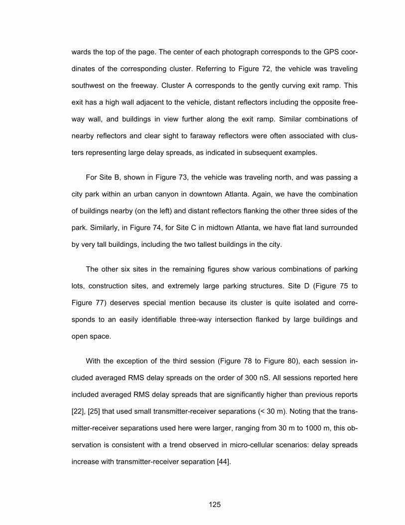
125

wards the top of the page. The center of each photograph corresponds to the GPS coor-

dinates of the corresponding cluster. Referring to Figure 72, the vehicle was traveling

southwest on the freeway. Cluster A corresponds to the gently curving exit ramp. This

exit has a high wall adjacent to the vehicle, distant reflectors including the opposite free-

way wall, and buildings in view further along the exit ramp. Similar combinations of

nearby reflectors and clear sight to faraway reflectors were often associated with clus-

ters representing large delay spreads, as indicated in subsequent examples.

For Site B, shown in Figure 73, the vehicle was traveling north, and was passing a

city park within an urban canyon in downtown Atlanta. Again, we have the combination

of buildings nearby (on the left) and distant reflectors flanking the other three sides of the

park. Similarly, in Figure 74, for Site C in midtown Atlanta, we have flat land surrounded

by very tall buildings, including the two tallest buildings in the city.

The other six sites in the remaining figures show various combinations of parking

lots, construction sites, and extremely large parking structures. Site D (Figure 75 to

Figure 77) deserves special mention because its cluster is quite isolated and corre-

sponds to an easily identifiable three-way intersection flanked by large buildings and

open space.

With the exception of the third session (Figure 78 to Figure 80), each session in-

cluded averaged RMS delay spreads on the order of 300 nS. All sessions reported here

included averaged RMS delay spreads that are significantly higher than previous reports

[22], [25] that used small transmitter-receiver separations (< 30 m). Noting that the trans-

mitter-receiver separations used here were larger, ranging from 30 m to 1000 m, this ob-

servation is consistent with a trend observed in micro-cellular scenarios: delay spreads

increase with transmitter-receiver separation [44].

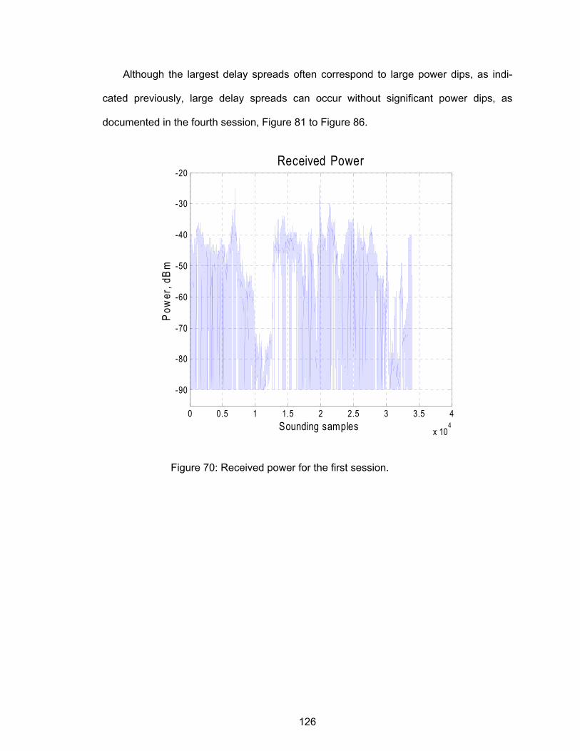
126

Although the largest delay spreads often correspond to large power dips, as indi-

cated previously, large delay spreads can occur without significant power dips, as

documented in the fourth session, Figure 81 to Figure 86.

0 0.5 1 1.5 2 2.5 3 3.5 4

x 104

-90

-80

-70

-60

-50

-40

-30

-20Received Power

Pow

er, d

Bm

Sounding samples

Figure 70: Received power for the first session.

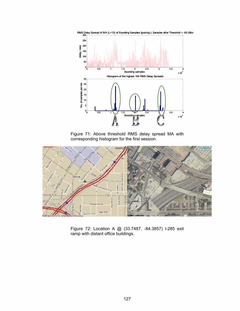
127

0 0.5 1 1.5 2 2.5 3 3.5 4

x 104

0

50

100

150

200

250

300RMS Delay Spread of MA (L=10) of Sounding Samples Ignoring L Samples after Threshold = -90 dBm

dela

y, n

sec

Sounding samples

0 0.5 1 1.5 2 2.5 3 3.5 4

x 104

0

5

10

15

20

25

30Histogram of the highest 100 RMS Delay Spreads

No.

of s

ampl

es p

er b

in

Sounding samples

0 0.5 1 1.5 2 2.5 3 3.5 4

x 104

0

50

100

150

200

250


dela

y, n

sec

Sounding samples

0 0.5 1 1.5 2 2.5 3 3.5 4

x 104

0

5

10

15

20

25


No.

of s

ampl

es p

er b

in

Sounding samples

Figure 71: Above threshold RMS delay spread MA with corresponding histogram for the first session.

Figure 72: Location A @ (33.7487, -84.3857) I-285 exit ramp with distant office buildings.

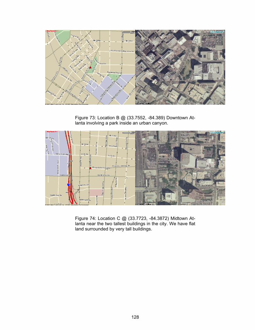
128

Figure 73: Location B @ (33.7552, -84.389) Downtown At-lanta involving a park inside an urban canyon.

Figure 74: Location C @ (33.7723, -84.3872) Midtown At-lanta near the two tallest buildings in the city. We have flat land surrounded by very tall buildings.

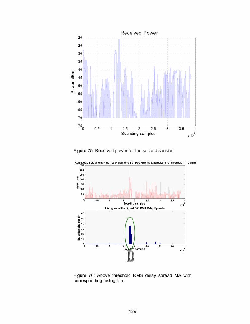
129

0 0.5 1 1.5 2 2.5 3 3.5 4

x 104

-75

-70

-65

-60

-55

-50

-45

-40

-35

-30

-25

-20Received Power

Pow

er, d

Bm

Sounding samples

Figure 75: Received power for the second session.

0 0.5 1 1.5 2 2.5 3 3.5 4

x 104

0

50

100

150

200

250

300


dela

y, n

sec

Sounding samples

0 0.5 1 1.5 2 2.5 3 3.5 4

x 104

0

10

20

30

40

50

60

Histogram of the highest 100 RMS Delay Spreads

No.

of s

ampl

es p

er b

in

Sounding samples

0 0.5 1 1.5 2 2.5 3 3.5 4

x 104

0

50

100

150

200

250

300


dela

y, n

sec

Sounding samples

0 0.5 1 1.5 2 2.5 3 3.5 4

x 104

0

10

20

30

40

50

60

Histogram of the highest 100 RMS Delay Spreads

No.

of s

ampl

es p

er b

in

Sounding samples

Figure 76: Above threshold RMS delay spread MA with corresponding histogram.

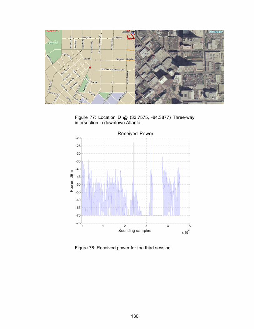
130

Figure 77: Location D @ (33.7575, -84.3877) Three-way intersection in downtown Atlanta.

0 1 2 3 4 5

x 104

-75

-70

-65

-60

-55

-50

-45

-40

-35

-30

-25

-20Received Power

Pow

er, d

Bm

Sounding samples

Figure 78: Received power for the third session.

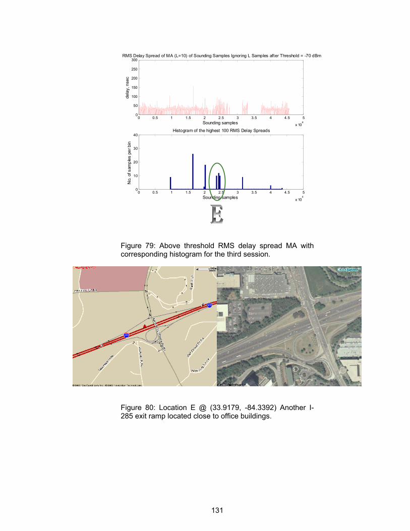
131

0 0.5 1 1.5 2 2.5 3 3.5 4 4.5 5

x 104

0

50

100

150

200

250


dela

y, n

sec

Sounding samples

0 0.5 1 1.5 2 2.5 3 3.5 4 4.5 5

x 104

0

10

20

30


No.

of s

ampl

es p

er b

in

Sounding samples

Figure 79: Above threshold RMS delay spread MA with corresponding histogram for the third session.

Figure 80: Location E @ (33.9179, -84.3392) Another I-285 exit ramp located close to office buildings.

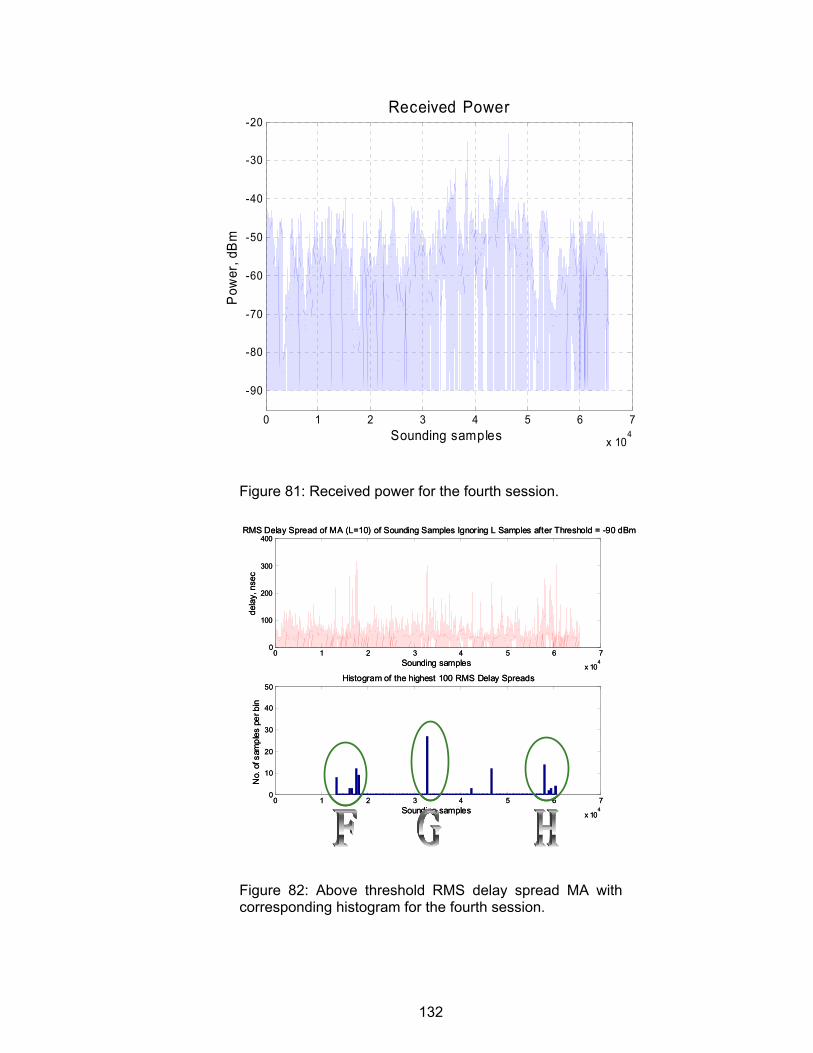
132

0 1 2 3 4 5 6 7

x 104

-90

-80

-70

-60

-50

-40

-30

-20Received Power

Pow

er, d

Bm

Sounding samples

Figure 81: Received power for the fourth session.

0 1 2 3 4 5 6 7

x 104

0

100

200

300


dela

y, n

sec

Sounding samples

0 1 2 3 4 5 6 7

x 104

0

10

20

30

40


No.

of s

ampl

es p

er b

in

Sounding samples

0 1 2 3 4 5 6 7

x 104

0

100

200

300


dela

y, n

sec

Sounding samples

0 1 2 3 4 5 6 7

x 104

0

10

20

30

40


No.

of s

ampl

es p

er b

in

Sounding samples

Figure 82: Above threshold RMS delay spread MA with corresponding histogram for the fourth session.

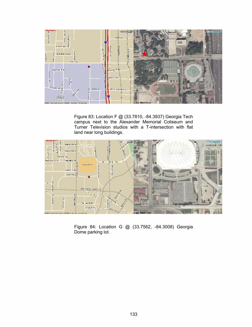
133

Figure 83: Location F @ (33.7810, -84.3937) Georgia Tech campus next to the Alexander Memorial Coliseum and Turner Television studios with a T-intersection with flat land near long buildings.

Figure 84: Location G @ (33.7562, -84.3008) Georgia Dome parking lot.

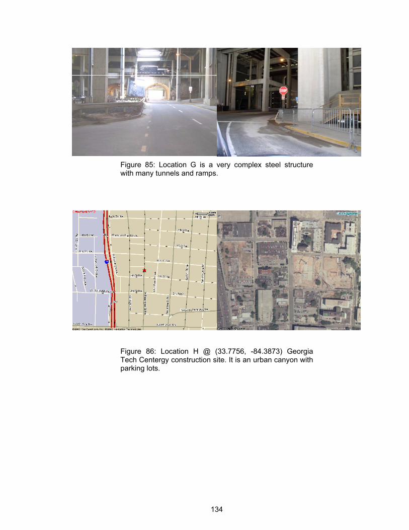
134

Figure 85: Location G is a very complex steel structure with many tunnels and ramps.

Figure 86: Location H @ (33.7756, -84.3873) Georgia Tech Centergy construction site. It is an urban canyon with parking lots.

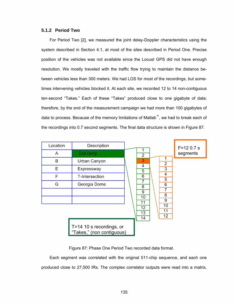
135

5.1.2 Period Two

For Period Two [2], we measured the joint delay-Doppler characteristics using the

system described in Section 4.1, at most of the sites described in Period One. Precise

position of the vehicles was not available since the Locust GPS did not have enough

resolution. We mostly traveled with the traffic flow trying to maintain the distance be-

tween vehicles less than 300 meters. We had LOS for most of the recordings, but some-

times intervening vehicles blocked it. At each site, we recorded 12 to 14 non-contiguous

ten-second “Takes.” Each of these “Takes” produced close to one gigabyte of data;

therefore, by the end of the measurement campaign we had more than 100 gigabytes of

data to process. Because of the memory limitations of Matlab™, we had to break each of

the recordings into 0.7 second segments. The final data structure is shown in Figure 87.

Figure 87: Phase One Period Two recorded data format.

Each segment was correlated with the original 511-chip sequence, and each one

produced close to 27,500 IRs. The complex correlator outputs were read into a matrix,

T=14 10 s recordings, or “Takes,” (non contiguous)

F=12 0.7 s segments

136

row by row, so that the matrix dimensions were 27,500 511× . Therefore, the columns of

this matrix correspond to 50 ns “delay bins.” Because there was no absolute time refer-

ence, there was no way to determine the absolute excess delay of the bins. However,

the relative excess delays of the bins were known. Furthermore, because of the long

length of the sequence (25.5 μs) and the usually small delay spreads of the MTM chan-

nel (on the order of 300 ns), it was easy to locate the consecutive bins with energy be-

cause the vast majority of bins were empty. By averaging the squared magnitudes of the

correlator outputs down each column of the matrix, we could obtain power delay profiles

for each 0.7 seconds segment.

5.2 Phase Two: 5.9 GHz Measurement Campaign For Phase Two, we measured three main environments: Urban Canyon, Suburban

Expressway, and Suburban Surface Street, and for each one, we had two types of links:

MTM and roadside-to-mobile (RTM). Each combination of link type and environment de-

fined a “scenario” from which we could develop a particular model.

For each scenario, we recorded several “Takes.” Each “Take” was 9.6 seconds

long, and we divided each one into 16 0.6 second segments. Each recorded segment

was split into its MLS and OFDM parts. Similarly to Phase One, the MLS part was corre-

lated to the chip sequence, and the output of the correlator was arranged into an impulse

response matrix such that each row was a channel IR taken at a certain time (i.e. certain

position of the cars) and each column represented a particular delay in the impulse re-

sponse. For the Phase Two MLS part, the matrix dimensions for each 0.6 second seg-

ment were approximately 5,500 511× , and they corresponded to 100 ns “delay bins.”

For the OFDM section, the number of columns was 512, and they corresponded to 50 ns

“delay bins.”

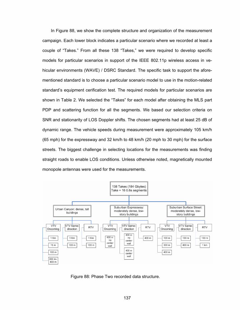
137

In Figure 88, we show the complete structure and organization of the measurement

campaign. Each lower block indicates a particular scenario where we recorded at least a

couple of “Takes.” From all these 138 “Takes,” we were required to develop specific

models for particular scenarios in support of the IEEE 802.11p wireless access in ve-

hicular environments (WAVE) / DSRC Standard. The specific task to support the afore-

mentioned standard is to choose a particular scenario model to use in the motion-related

standard’s equipment cerification test. The required models for particular scenarios are

shown in Table 2. We selected the “Takes” for each model after obtaining the MLS part

PDP and scattering function for all the segments. We based our selection criteria on

SNR and stationarity of LOS Doppler shifts. The chosen segments had at least 25 dB of

dynamic range. The vehicle speeds during measurement were approximately 105 km/h

(65 mph) for the expressway and 32 km/h to 48 km/h (20 mph to 30 mph) for the surface

streets. The biggest challenge in selecting locations for the measurements was finding

straight roads to enable LOS conditions. Unless otherwise noted, magnetically mounted

monopole antennas were used for the measurements.

Figure 88: Phase Two recorded data structure.

138

Table 2: Description of the locations for each scenario

Scenario Date Location Takes MTM - Expressway Oncoming, 300-400 m 04/19/2006 GA 675 between exits 5 and 7 4

RTM - Urban Canyon 100 m 04/24/2006 Approach Peachtree Street at Col-ony Square from the North 4

Westbound GA 78 4 RTM - Expressway 300-400 m 04/25/2006 Eastbound GA 78 4 04/12/2006 Along Edgewood Avenue 2 MTM - Urban Canyon Oncom-

ing 100 m 04/25/2006 Along Edgewood Avenue 2

RTM - Suburban Street 100 m 04/25/2006 Four different approaches to Me-morial Drive and Candler Road 10

Along North I-285 7 04/19/2006 West on I-20 6 I-285 @ Ashford Dunwoody 4

MTM - Expressway Same Di-rection With Wall, 300-400 m 04/17/2006 GA 400 North, just north of I-285 4

In the rest of this section, we present a brief description of each of the scenarios

chosen for Phase Two. In each one, we show a representative photo of the scenario, the

particularities encountered, and any other specific information necessary.

• MTM - Expressway Oncoming, 300-400 m Scenario

For this scenario, we found a stretch of highway without a middle wall at GA 675 be-

tween exits 5 and 7. For the measurement, we synchronized each of the vehicles so that

they entered the highway at the same time. We then accelerated each one to 65 mph,

and it was at that instance that we began recording. The recording or “Take” period

sometimes allowed for the vehicles to cross or pass each other. We were able to obtain

four good “Takes,” i.e., good SNR, vehicle speeds, etc. From the total 64 0.6 second

segments, we only chose the ones that represented a vehicle separation of 300-400 m

for processing. We found these segments either by looking at their Doppler spectrum or

by using the notes taken. These particular segments showed a fixed LOS Doppler shift

in the first tap spectrum. In Figure 89, we show an instance when we had the required

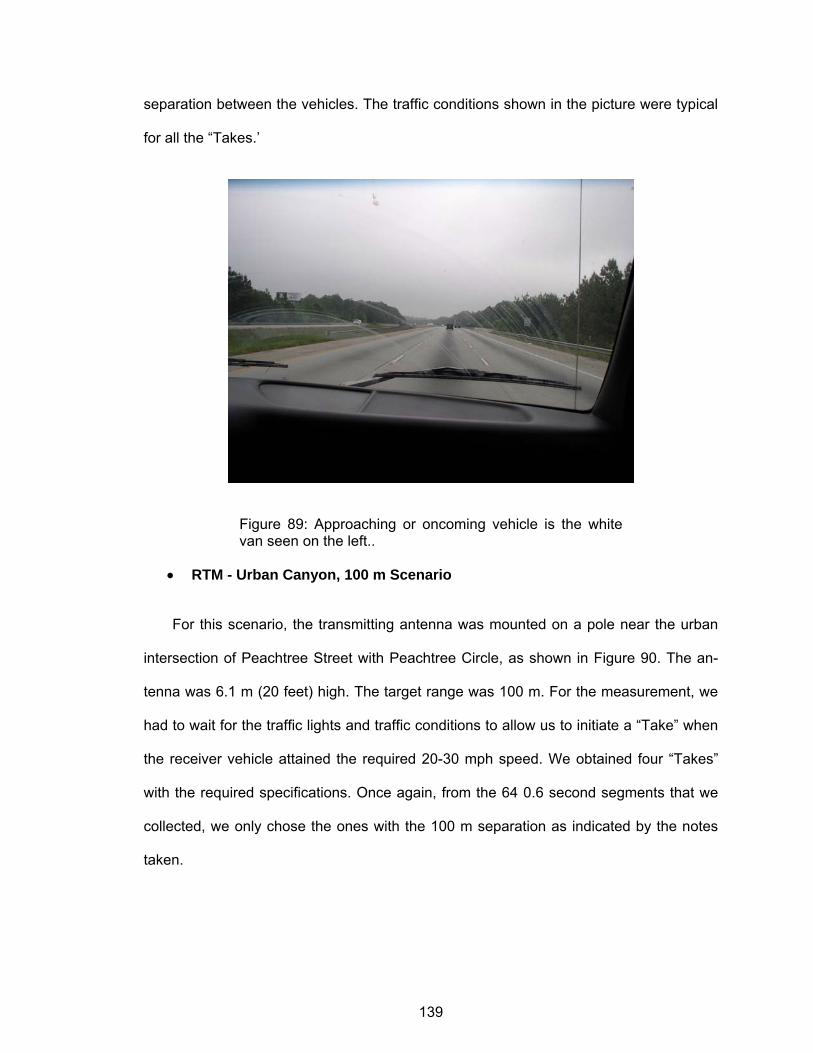
139

separation between the vehicles. The traffic conditions shown in the picture were typical

for all the “Takes.’

Figure 89: Approaching or oncoming vehicle is the white van seen on the left..

• RTM - Urban Canyon, 100 m Scenario

For this scenario, the transmitting antenna was mounted on a pole near the urban

intersection of Peachtree Street with Peachtree Circle, as shown in Figure 90. The an-

tenna was 6.1 m (20 feet) high. The target range was 100 m. For the measurement, we

had to wait for the traffic lights and traffic conditions to allow us to initiate a “Take” when

the receiver vehicle attained the required 20-30 mph speed. We obtained four “Takes”

with the required specifications. Once again, from the 64 0.6 second segments that we

collected, we only chose the ones with the 100 m separation as indicated by the notes

taken.

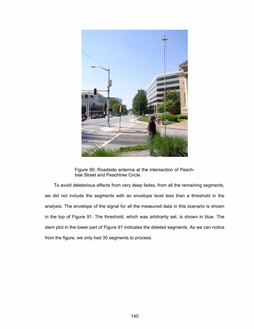
140

Figure 90: Roadside antenna at the intersection of Peach-tree Street and Peachtree Circle.

To avoid deleterious effects from very deep fades, from all the remaining segments,

we did not include the segments with an envelope level less than a threshold in the

analysis. The envelope of the signal for all the measured data in this scenario is shown

in the top of Figure 91. The threshold, which was arbitrarily set, is shown in blue. The

stem plot in the lower part of Figure 91 indicates the deleted segments. As we can notice

from the figure, we only had 30 segments to process.

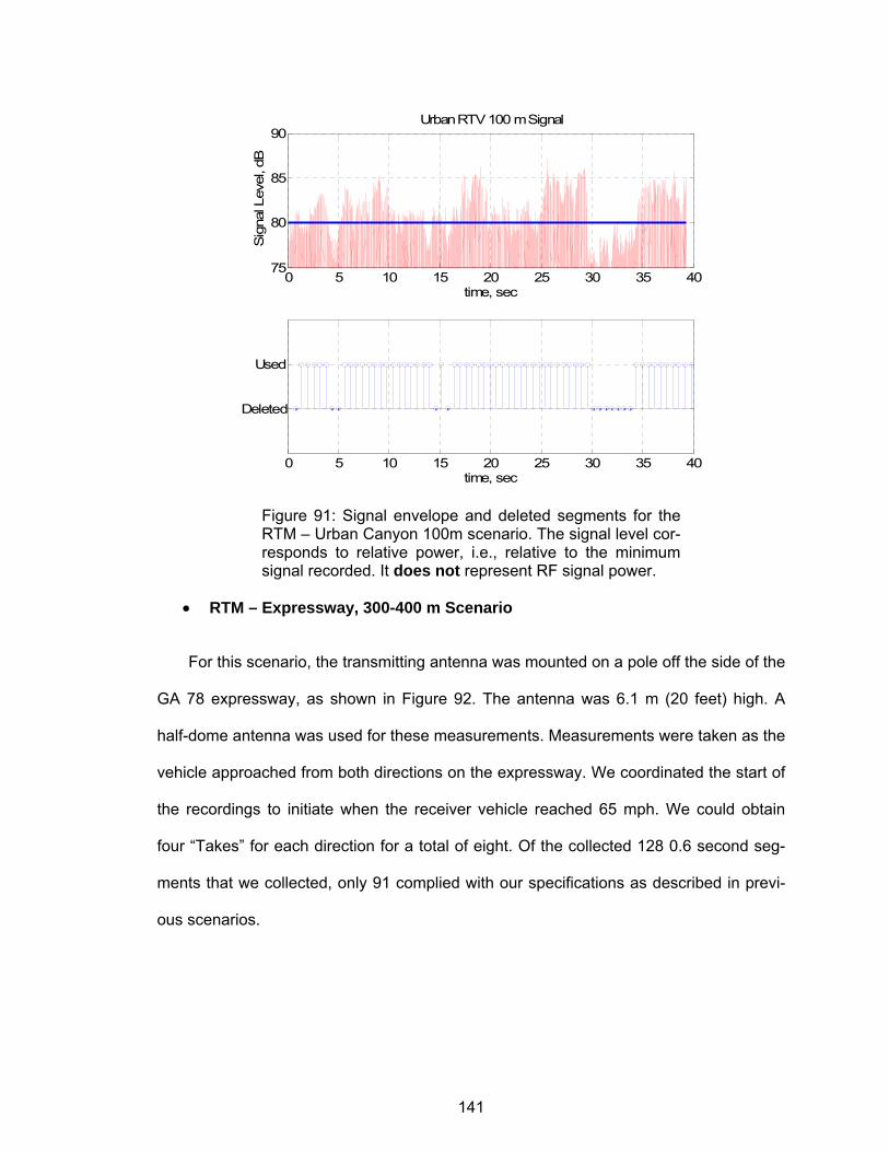
141

0 5 10 15 20 25 30 35 4075

80

85

90Urban RTV 100 m Signal

Sig

nal L

evel

, dB

time, sec

0 5 10 15 20 25 30 35 40

Deleted

Used

time, sec

Figure 91: Signal envelope and deleted segments for the RTM – Urban Canyon 100m scenario. The signal level cor-responds to relative power, i.e., relative to the minimum signal recorded. It does not represent RF signal power.

• RTM – Expressway, 300-400 m Scenario

For this scenario, the transmitting antenna was mounted on a pole off the side of the

GA 78 expressway, as shown in Figure 92. The antenna was 6.1 m (20 feet) high. A

half-dome antenna was used for these measurements. Measurements were taken as the

vehicle approached from both directions on the expressway. We coordinated the start of

the recordings to initiate when the receiver vehicle reached 65 mph. We could obtain

four “Takes” for each direction for a total of eight. Of the collected 128 0.6 second seg-

ments that we collected, only 91 complied with our specifications as described in previ-

ous scenarios.

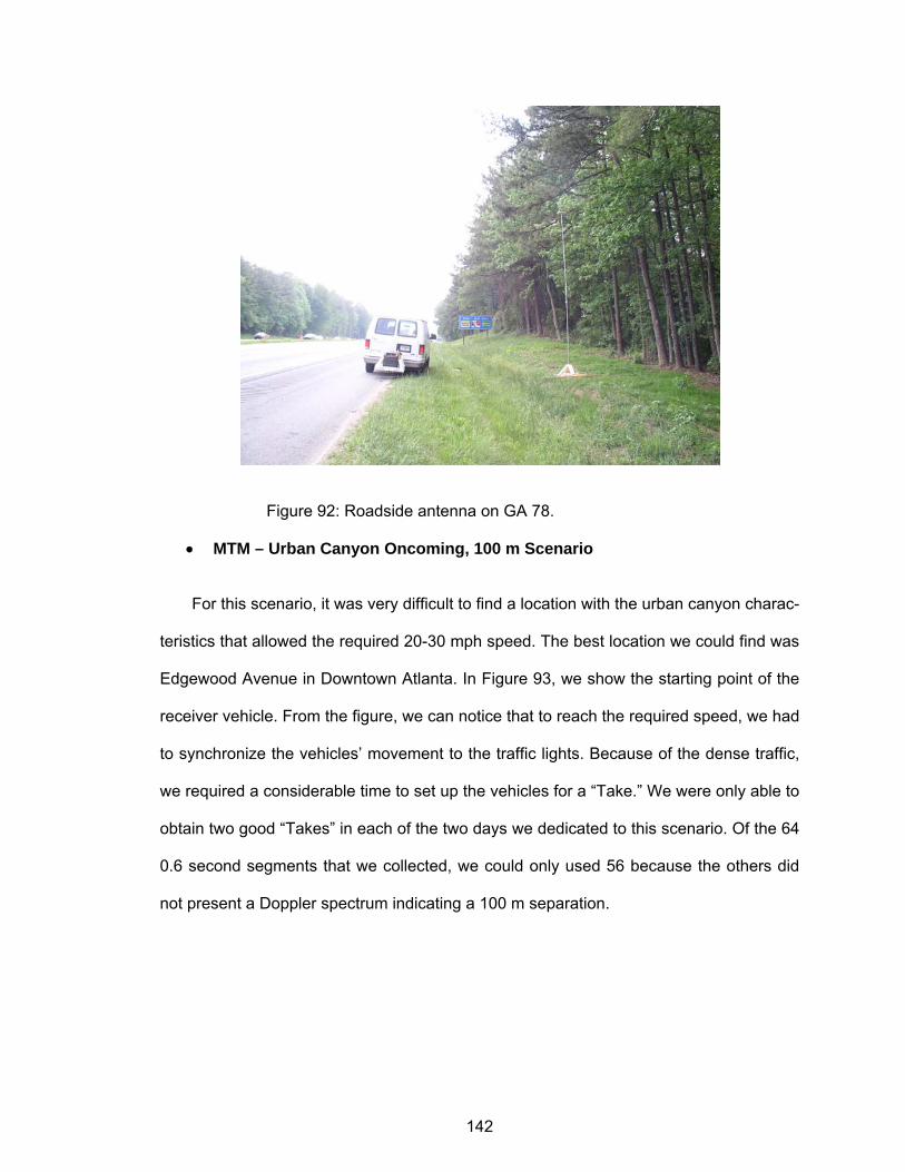
142

Figure 92: Roadside antenna on GA 78.

• MTM – Urban Canyon Oncoming, 100 m Scenario

For this scenario, it was very difficult to find a location with the urban canyon charac-

teristics that allowed the required 20-30 mph speed. The best location we could find was

Edgewood Avenue in Downtown Atlanta. In Figure 93, we show the starting point of the

receiver vehicle. From the figure, we can notice that to reach the required speed, we had

to synchronize the vehicles’ movement to the traffic lights. Because of the dense traffic,

we required a considerable time to set up the vehicles for a “Take.” We were only able to

obtain two good “Takes” in each of the two days we dedicated to this scenario. Of the 64

0.6 second segments that we collected, we could only used 56 because the others did

not present a Doppler spectrum indicating a 100 m separation.

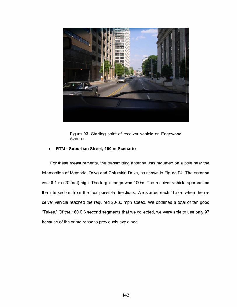
143

Figure 93: Starting point of receiver vehicle on Edgewood Avenue.

• RTM - Suburban Street, 100 m Scenario

For these measurements, the transmitting antenna was mounted on a pole near the

intersection of Memorial Drive and Columbia Drive, as shown in Figure 94. The antenna

was 6.1 m (20 feet) high. The target range was 100m. The receiver vehicle approached

the intersection from the four possible directions. We started each “Take” when the re-

ceiver vehicle reached the required 20-30 mph speed. We obtained a total of ten good

“Takes.” Of the 160 0.6 second segments that we collected, we were able to use only 97

because of the same reasons previously explained.

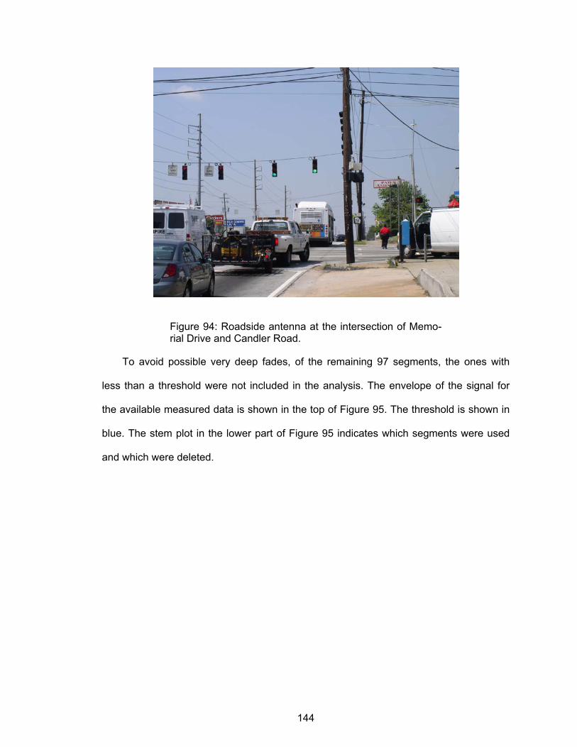
144

Figure 94: Roadside antenna at the intersection of Memo-rial Drive and Candler Road.

To avoid possible very deep fades, of the remaining 97 segments, the ones with

less than a threshold were not included in the analysis. The envelope of the signal for

the available measured data is shown in the top of Figure 95. The threshold is shown in

blue. The stem plot in the lower part of Figure 95 indicates which segments were used

and which were deleted.

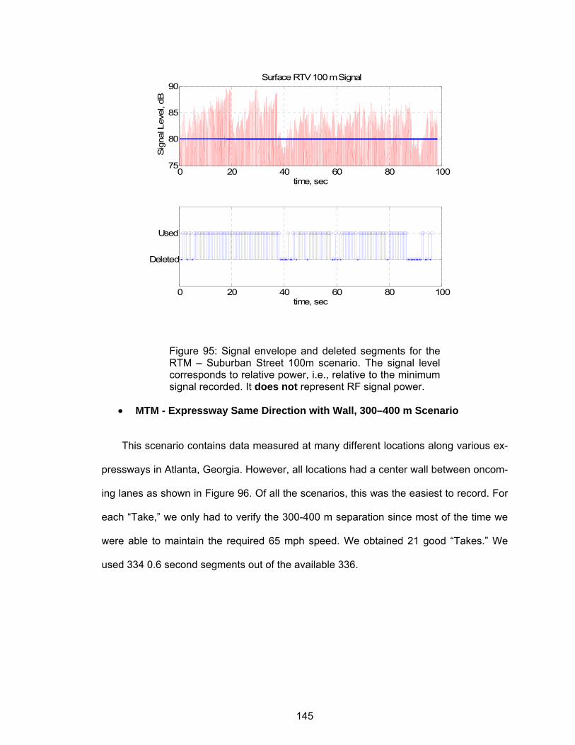
145

0 20 40 60 80 10075

80

85

90Surface RTV 100 m Signal

Sig

nal L

evel

, dB

time, sec

0 20 40 60 80 100

Deleted

Used

time, sec

Figure 95: Signal envelope and deleted segments for the RTM – Suburban Street 100m scenario. The signal level corresponds to relative power, i.e., relative to the minimum signal recorded. It does not represent RF signal power.

• MTM - Expressway Same Direction with Wall, 300–400 m Scenario

This scenario contains data measured at many different locations along various ex-

pressways in Atlanta, Georgia. However, all locations had a center wall between oncom-

ing lanes as shown in Figure 96. Of all the scenarios, this was the easiest to record. For

each “Take,” we only had to verify the 300-400 m separation since most of the time we

were able to maintain the required 65 mph speed. We obtained 21 good “Takes.” We

used 334 0.6 second segments out of the available 336.

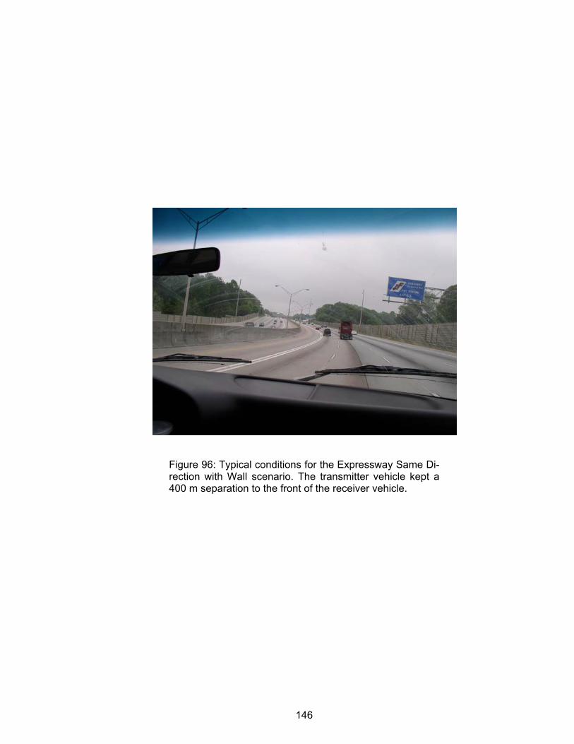
146

Figure 96: Typical conditions for the Expressway Same Di-rection with Wall scenario. The transmitter vehicle kept a 400 m separation to the front of the receiver vehicle.

147

CHAPTER 6

MEASUREMENT RESULTS AND CHANNEL MODELING

In this chapter, we used one common scenario from each of the two measurement

campaigns to describe how we develop the final product of this investigation, which is a

reliable channel model to use either in simulation or a channel emulator. The most simi-

lar scenarios that we found were the Location E Expressway from Phase One and the

Suburban Expressway MTM Same Direction Wall from Phase Two. We have to clarify at

this point that the modeling process presented in this chapter has been progressive, i.e.,

for the second phase, we started the modeling process including all the previous experi-

ence gained in the first phase. For Phase One, we concentrated our efforts in matching

the BER behavior between the recorded channel and our proposed synthesized chan-

nels. For the channel synthesis, we used the random noise filtering technique. From the

recorded channel, we obtained the number of taps, their delay, their power, and a filter

template. As we will describe in Section 6.1.2.4, we have learned two main lessons from

Phase One channel modeling. First, we have learned that even when a spectral tem-

plate clearly indicates a narrow frequency peak, as you would expect from a strong LOS

component, it does not produce a significant K-factor. Second, the BER performance

over the recorded channel clearly indicates that there is a strong relationship between

BER and the existence of a LOS component. For Phase Two, we developed a technique

to separate the random and deterministic parts of the recorded channel. Once we had

this separation, we used the random part to obtain the per-tap spectra. This time, in-

stead of using the obtained spectra as filter templates, we develop a spectrum fitting

148

procedure to use a combination of the four possible spectrum shapes we can find in ei-

ther a simulation system or a channel emulator. We used the deterministic part to pro-

duce the K-factor. For this second phase, instead of using a simulation system, we

tested our proposed models with hardware prototypes developed for the DSRC stan-

dard. Once again, we empirically noticed a strong relationship between the K-factor and,

for this phase, the packet error rate (PER) of the prototype sytem. This relationship sug-

gests that in order to have a more precise model, it is necessary to model the dynamics

of the K-factor.

6.1 Phase One Channel Modeling In the first of two parts of this section, we developed a channel model, which we

will call a statistical model, following the procedure of Section 2.3. In the second part, we

propose a new channel modeling method, which we named Partitioned Model, to com-

pensate the limitations encountered in the Statistical Model.

6.1.1 Statistical Model Develpment

We considered Mohr’s method [51] as our first approach for our model develop-

ment. This method considers direct averaging of the extracted model parameters to ob-

tain the overall model parameters. As we shall demonstrate, this approach is far from

satisfactory to comply with the performance extremes encountered in the real or re-

corded channel. To justify this claim, we developed a system simulation tool capable of

measuring the performance of a real or synthesized channel.

6.1.1.1 Resulting Tap Characteristics

For the expressway location, we recorded 14 ten-second “Takes.” We divided each

take into 12 0.7-second segments for their analysis. Please note that each “Take” corre-

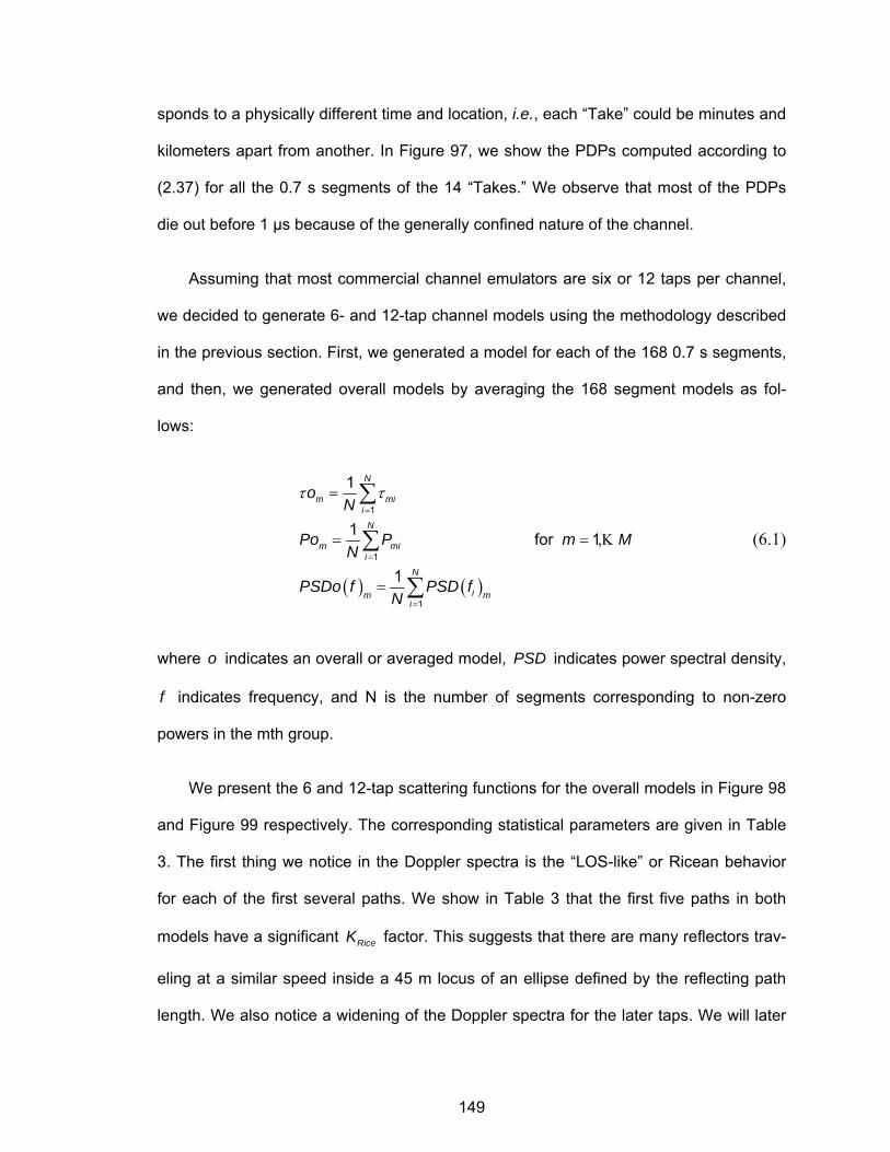
149

sponds to a physically different time and location, i.e., each “Take” could be minutes and

kilometers apart from another. In Figure 97, we show the PDPs computed according to

(2.37) for all the 0.7 s segments of the 14 “Takes.” We observe that most of the PDPs

die out before 1 μs because of the generally confined nature of the channel.

Assuming that most commercial channel emulators are six or 12 taps per channel,

we decided to generate 6- and 12-tap channel models using the methodology described

in the previous section. First, we generated a model for each of the 168 0.7 s segments,

and then, we generated overall models by averaging the 168 segment models as fol-

lows:

( ) ( )

τ τ=

=

=

=

= =

=

∑

∑

∑

K

1

1

1

1

1 for 1,

1

N

m mii

N

m mii

N

im mi

oN

Po P m MN

PSDo f PSD fN

(6.1)

where o indicates an overall or averaged model, PSD indicates power spectral density,

f indicates frequency, and N is the number of segments corresponding to non-zero

powers in the mth group.

We present the 6 and 12-tap scattering functions for the overall models in Figure 98

and Figure 99 respectively. The corresponding statistical parameters are given in Table

3. The first thing we notice in the Doppler spectra is the “LOS-like” or Ricean behavior

for each of the first several paths. We show in Table 3 that the first five paths in both

models have a significant RiceK factor. This suggests that there are many reflectors trav-

eling at a similar speed inside a 45 m locus of an ellipse defined by the reflecting path

length. We also notice a widening of the Doppler spectra for the later taps. We will later

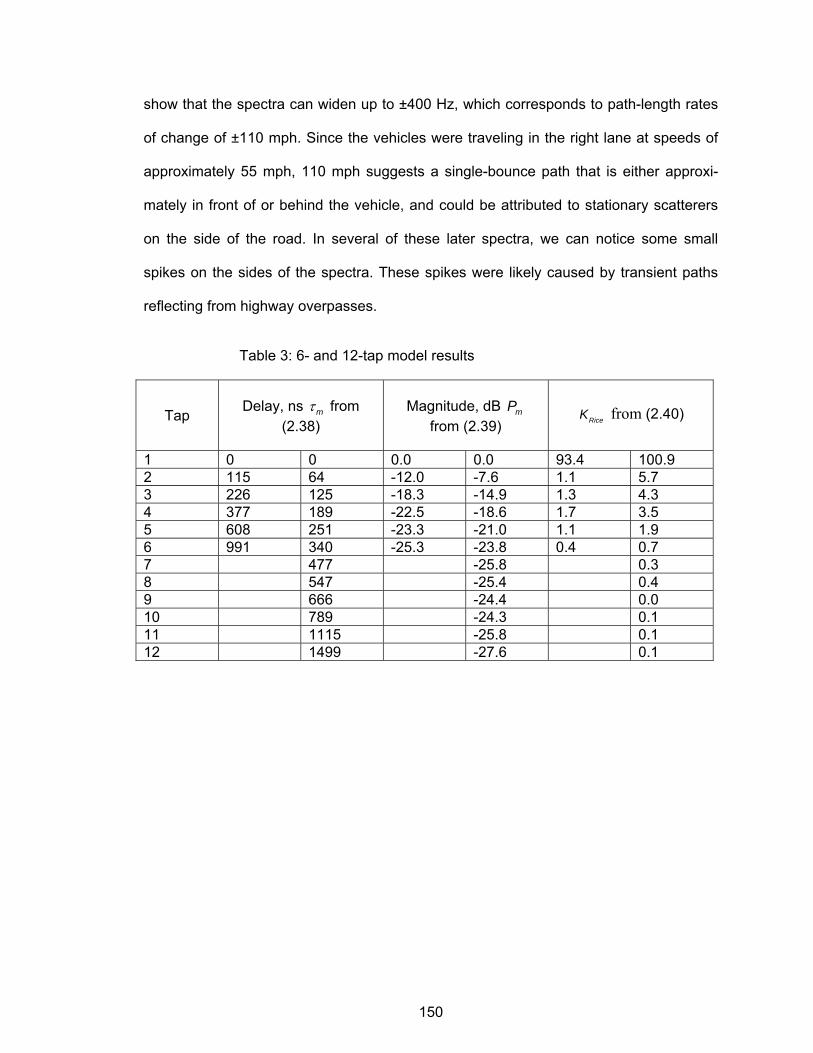
150

show that the spectra can widen up to ±400 Hz, which corresponds to path-length rates

of change of ±110 mph. Since the vehicles were traveling in the right lane at speeds of

approximately 55 mph, 110 mph suggests a single-bounce path that is either approxi-

mately in front of or behind the vehicle, and could be attributed to stationary scatterers

on the side of the road. In several of these later spectra, we can notice some small

spikes on the sides of the spectra. These spikes were likely caused by transient paths

reflecting from highway overpasses.

Table 3: 6- and 12-tap model results

Tap Delay, ns τm from (2.38)

Magnitude, dB mP from (2.39) RiceK from (2.40)

1 0 0 0.0 0.0 93.4 100.9 2 115 64 -12.0 -7.6 1.1 5.7 3 226 125 -18.3 -14.9 1.3 4.3 4 377 189 -22.5 -18.6 1.7 3.5 5 608 251 -23.3 -21.0 1.1 1.9 6 991 340 -25.3 -23.8 0.4 0.7 7 477 -25.8 0.3 8 547 -25.4 0.4 9 666 -24.4 0.0 10 789 -24.3 0.1 11 1115 -25.8 0.1 12 1499 -27.6 0.1

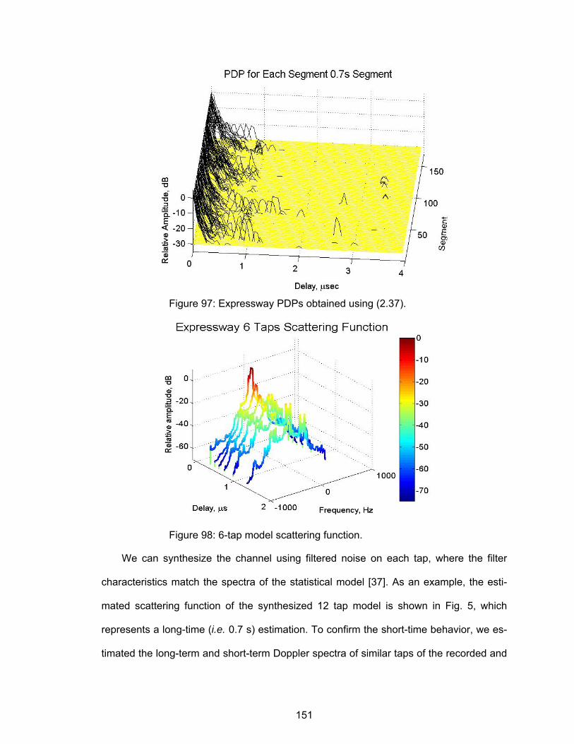
151

Figure 97: Expressway PDPs obtained using (2.37).

Figure 98: 6-tap model scattering function.

We can synthesize the channel using filtered noise on each tap, where the filter

characteristics match the spectra of the statistical model [37]. As an example, the esti-

mated scattering function of the synthesized 12 tap model is shown in Fig. 5, which

represents a long-time (i.e. 0.7 s) estimation. To confirm the short-time behavior, we es-

timated the long-term and short-term Doppler spectra of similar taps of the recorded and

152

synthesized channel. For the long-time spectrum, we used the approximately 27,000 IRs

in 0.7 s for the estimate, and for the short-time spectra, we obtained the estimate every

2,048 IRs or approximately every 50 ns. In Figure 101, we show the resulting Doppler

spectra for the third tap of the synthesized model. In Figure 102, we present the results

of a latter tap of one 0.7-second segment of one of the “Takes” of the recorded channel.

As we can see in these figures, the short-time spectra of the synthesized channel have

transient behavior similar to that of the real channel. We can also notice a spectra wid-

ening up to 400 Hz.

Figure 99: 12-tap model scattering function.

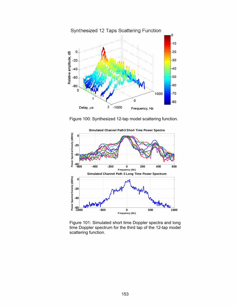
153

Figure 100: Synthesized 12-tap model scattering function.

Figure 101: Simulated short time Doppler spectra and long time Doppler spectrum for the third tap of the 12-tap model scattering function.

-600 -400 -200 0 200 400 600-60

-40

-20

0

Pow

er S

pect

ral D

ensi

ty (d

B/Hz

)

Frequency (Hz)

Simulated Channel Path3 Short Time Power Spectra

-1000 -500 0 500 1000-60

-40

-20

0

Pow

er S

pect

ral D

ensi

ty (d

B/Hz

)

Frequency (Hz)

Simulated Channel Path 3 Long Time Power Spectrum

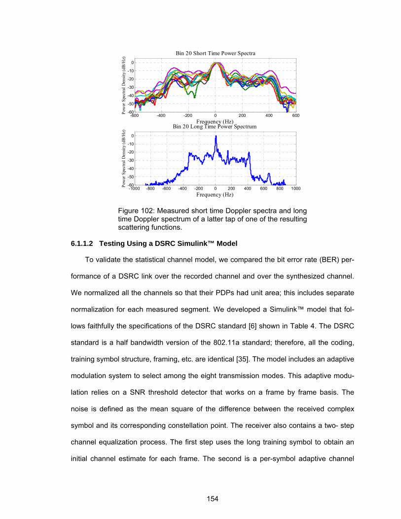
154

-600 -400 -200 0 200 400 600-60

-50

-40

-30

-20

-10

0

Pow

er S

pect

ral D

ensit

y (d

B/H

z)Frequency (Hz)

Bin 20 Short Time Power Spectra

-1000 -800 -600 -400 -200 0 200 400 600 800 1000-60

-50

-40

-30

-20

-10

0

Pow

er S

pect

ral D

ensit

y (d

B/H

z)

Frequency (Hz)

Bin 20 Long Time Power Spectrum

Figure 102: Measured short time Doppler spectra and long time Doppler spectrum of a latter tap of one of the resulting scattering functions.

6.1.1.2 Testing Using a DSRC Simulink™ Model

To validate the statistical channel model, we compared the bit error rate (BER) per-

formance of a DSRC link over the recorded channel and over the synthesized channel.

We normalized all the channels so that their PDPs had unit area; this includes separate

normalization for each measured segment. We developed a Simulink™ model that fol-

lows faithfully the specifications of the DSRC standard [6] shown in Table 4. The DSRC

standard is a half bandwidth version of the 802.11a standard; therefore, all the coding,

training symbol structure, framing, etc. are identical [35]. The model includes an adaptive

modulation system to select among the eight transmission modes. This adaptive modu-

lation relies on a SNR threshold detector that works on a frame by frame basis. The

noise is defined as the mean square of the difference between the received complex

symbol and its corresponding constellation point. The receiver also contains a two- step

channel equalization process. The first step uses the long training symbol to obtain an

initial channel estimate for each frame. The second is a per-symbol adaptive channel

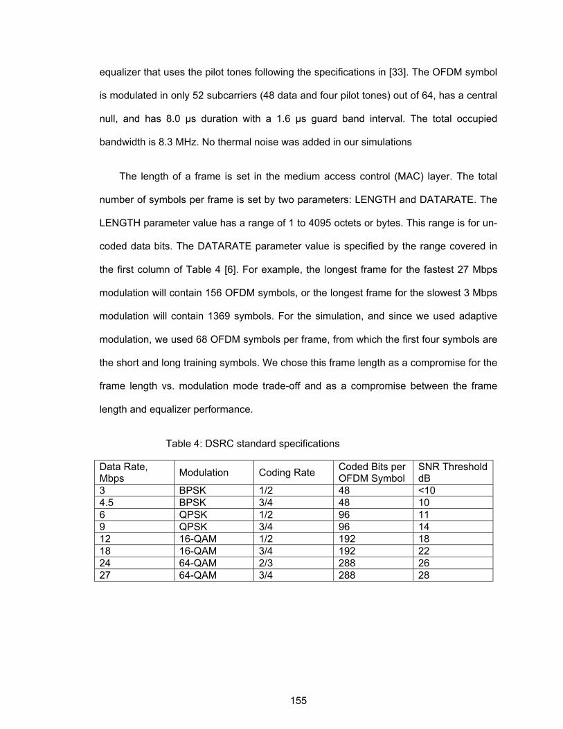
155

equalizer that uses the pilot tones following the specifications in [33]. The OFDM symbol

is modulated in only 52 subcarriers (48 data and four pilot tones) out of 64, has a central

null, and has 8.0 μs duration with a 1.6 μs guard band interval. The total occupied

bandwidth is 8.3 MHz. No thermal noise was added in our simulations

The length of a frame is set in the medium access control (MAC) layer. The total

number of symbols per frame is set by two parameters: LENGTH and DATARATE. The

LENGTH parameter value has a range of 1 to 4095 octets or bytes. This range is for un-

coded data bits. The DATARATE parameter value is specified by the range covered in

the first column of Table 4 [6]. For example, the longest frame for the fastest 27 Mbps

modulation will contain 156 OFDM symbols, or the longest frame for the slowest 3 Mbps

modulation will contain 1369 symbols. For the simulation, and since we used adaptive

modulation, we used 68 OFDM symbols per frame, from which the first four symbols are

the short and long training symbols. We chose this frame length as a compromise for the

frame length vs. modulation mode trade-off and as a compromise between the frame

length and equalizer performance.

Table 4: DSRC standard specifications

Data Rate, Mbps Modulation Coding Rate Coded Bits per

OFDM Symbol SNR Threshold dB

3 BPSK 1/2 48 <10 4.5 BPSK 3/4 48 10 6 QPSK 1/2 96 11 9 QPSK 3/4 96 14 12 16-QAM 1/2 192 18 18 16-QAM 3/4 192 22 24 64-QAM 2/3 288 26 27 64-QAM 3/4 288 28

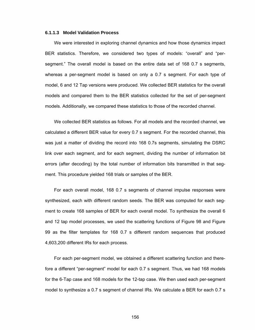
156

6.1.1.3 Model Validation Process

We were interested in exploring channel dynamics and how those dynamics impact

BER statistics. Therefore, we considered two types of models: “overall” and “per-

segment.” The overall model is based on the entire data set of 168 0.7 s segments,

whereas a per-segment model is based on only a 0.7 s segment. For each type of

model, 6 and 12 Tap versions were produced. We collected BER statistics for the overall

models and compared them to the BER statistics collected for the set of per-segment

models. Additionally, we compared these statistics to those of the recorded channel.

We collected BER statistics as follows. For all models and the recorded channel, we

calculated a different BER value for every 0.7 s segment. For the recorded channel, this

was just a matter of dividing the record into 168 0.7s segments, simulating the DSRC

link over each segment, and for each segment, dividing the number of information bit

errors (after decoding) by the total number of information bits transmitted in that seg-

ment. This procedure yielded 168 trials or samples of the BER.

For each overall model, 168 0.7 s segments of channel impulse responses were

synthesized, each with different random seeds. The BER was computed for each seg-

ment to create 168 samples of BER for each overall model. To synthesize the overall 6

and 12 tap model processes, we used the scattering functions of Figure 98 and Figure

99 as the filter templates for 168 0.7 s different random sequences that produced

4,603,200 different IRs for each process.

For each per-segment model, we obtained a different scattering function and there-

fore a different “per-segment” model for each 0.7 s segment. Thus, we had 168 models

for the 6-Tap case and 168 models for the 12-tap case. We then used each per-segment

model to synthesize a 0.7 s segment of channel IRs. We calculate a BER for each 0.7 s

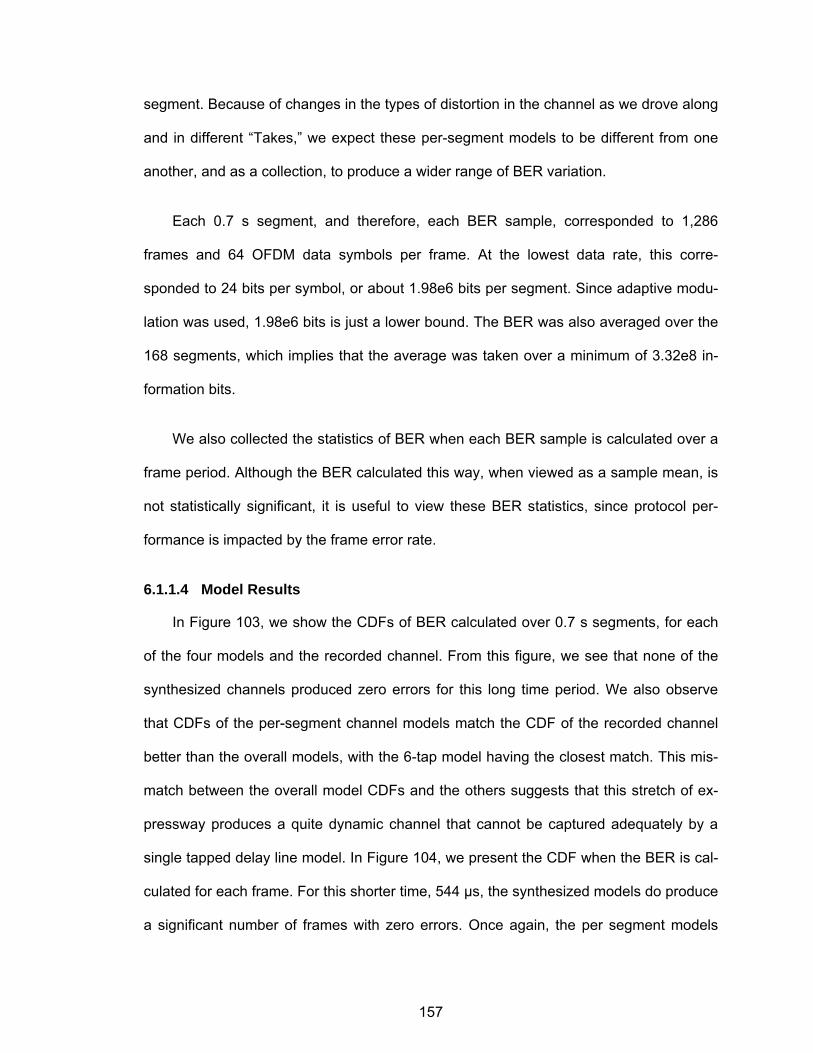
157

segment. Because of changes in the types of distortion in the channel as we drove along

and in different “Takes,” we expect these per-segment models to be different from one

another, and as a collection, to produce a wider range of BER variation.

Each 0.7 s segment, and therefore, each BER sample, corresponded to 1,286

frames and 64 OFDM data symbols per frame. At the lowest data rate, this corre-

sponded to 24 bits per symbol, or about 1.98e6 bits per segment. Since adaptive modu-

lation was used, 1.98e6 bits is just a lower bound. The BER was also averaged over the

168 segments, which implies that the average was taken over a minimum of 3.32e8 in-

formation bits.

We also collected the statistics of BER when each BER sample is calculated over a

frame period. Although the BER calculated this way, when viewed as a sample mean, is

not statistically significant, it is useful to view these BER statistics, since protocol per-

formance is impacted by the frame error rate.

6.1.1.4 Model Results

In Figure 103, we show the CDFs of BER calculated over 0.7 s segments, for each

of the four models and the recorded channel. From this figure, we see that none of the

synthesized channels produced zero errors for this long time period. We also observe

that CDFs of the per-segment channel models match the CDF of the recorded channel

better than the overall models, with the 6-tap model having the closest match. This mis-

match between the overall model CDFs and the others suggests that this stretch of ex-

pressway produces a quite dynamic channel that cannot be captured adequately by a

single tapped delay line model. In Figure 104, we present the CDF when the BER is cal-

culated for each frame. For this shorter time, 544 μs, the synthesized models do produce

a significant number of frames with zero errors. Once again, the per segment models

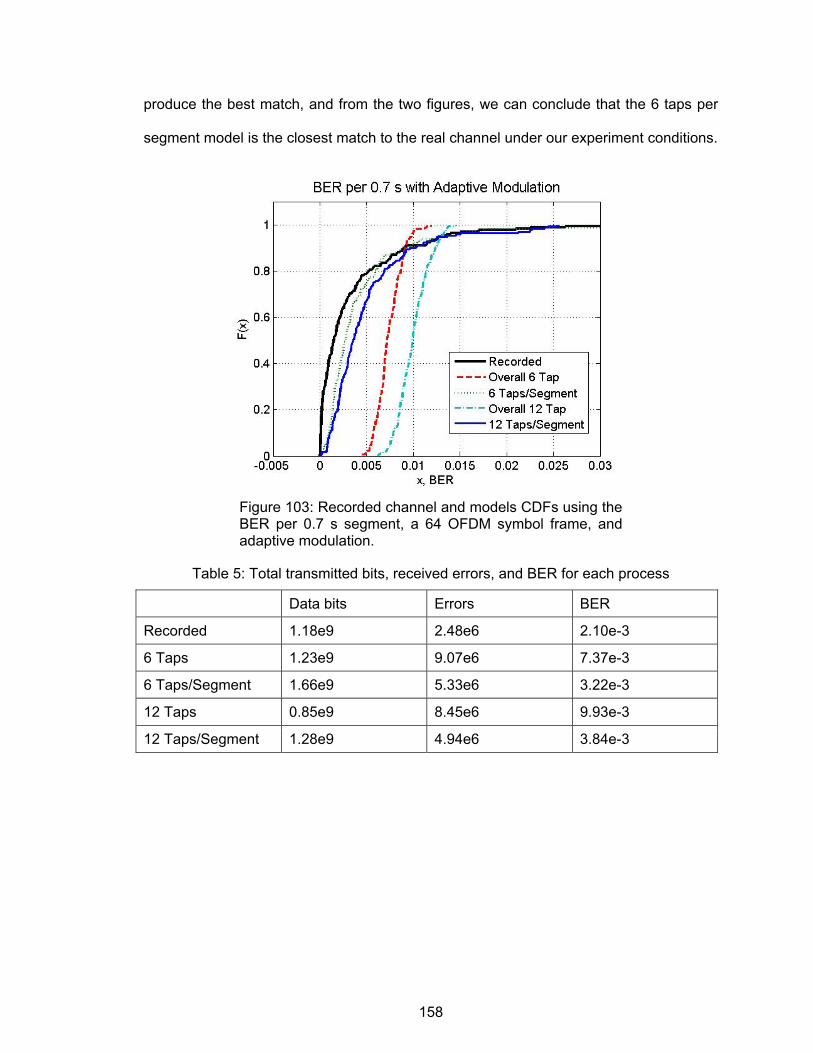
158

produce the best match, and from the two figures, we can conclude that the 6 taps per

segment model is the closest match to the real channel under our experiment conditions.

Figure 103: Recorded channel and models CDFs using the BER per 0.7 s segment, a 64 OFDM symbol frame, and adaptive modulation.

Table 5: Total transmitted bits, received errors, and BER for each process

Data bits Errors BER

Recorded 1.18e9 2.48e6 2.10e-3

6 Taps 1.23e9 9.07e6 7.37e-3

6 Taps/Segment 1.66e9 5.33e6 3.22e-3

12 Taps 0.85e9 8.45e6 9.93e-3

12 Taps/Segment 1.28e9 4.94e6 3.84e-3

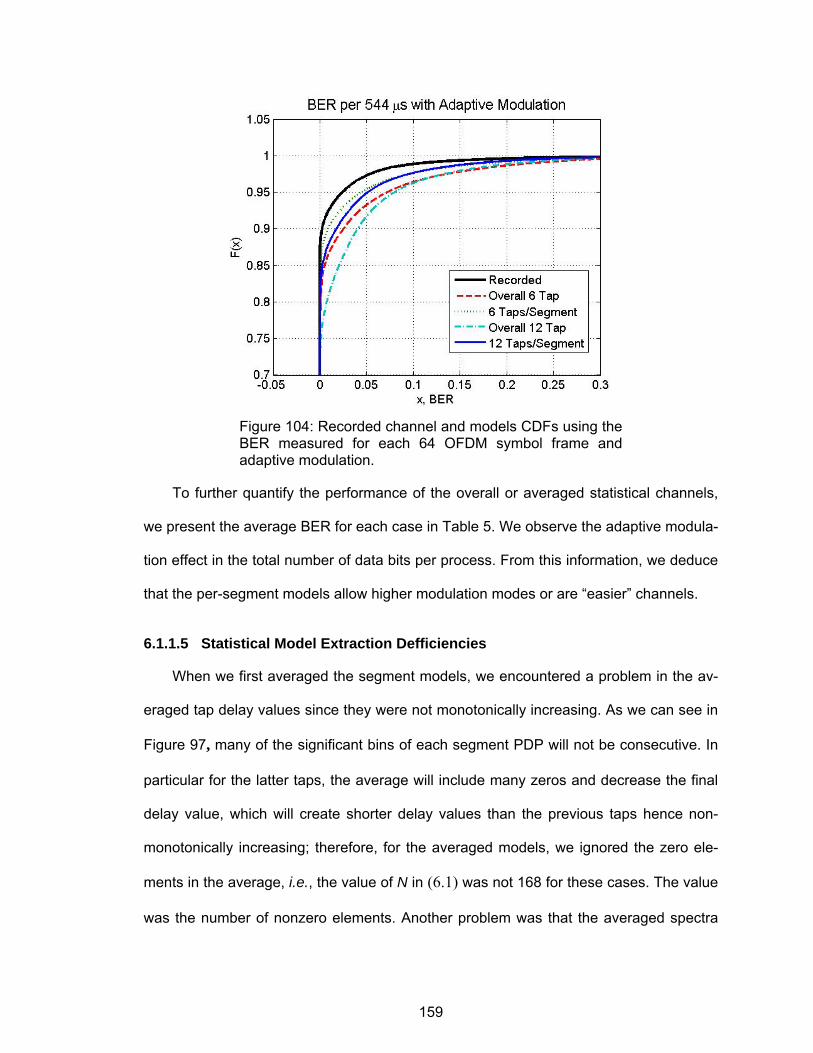
159

Figure 104: Recorded channel and models CDFs using the BER measured for each 64 OFDM symbol frame and adaptive modulation.

To further quantify the performance of the overall or averaged statistical channels,

we present the average BER for each case in Table 5. We observe the adaptive modula-

tion effect in the total number of data bits per process. From this information, we deduce

that the per-segment models allow higher modulation modes or are “easier” channels.

6.1.1.5 Statistical Model Extraction Defficiencies

When we first averaged the segment models, we encountered a problem in the av-

eraged tap delay values since they were not monotonically increasing. As we can see in

Figure 97, many of the significant bins of each segment PDP will not be consecutive. In

particular for the latter taps, the average will include many zeros and decrease the final

delay value, which will create shorter delay values than the previous taps hence non-

monotonically increasing; therefore, for the averaged models, we ignored the zero ele-

ments in the average, i.e., the value of N in (6.1) was not 168 for these cases. The value

was the number of nonzero elements. Another problem was that the averaged spectra

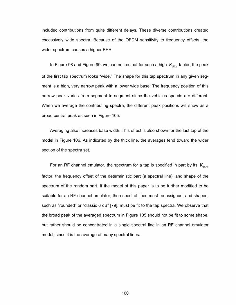
160

included contributions from quite different delays. These diverse contributions created

excessively wide spectra. Because of the OFDM sensitivity to frequency offsets, the

wider spectrum causes a higher BER.

In Figure 98 and Figure 99, we can notice that for such a high RiceK factor, the peak

of the first tap spectrum looks “wide.” The shape for this tap spectrum in any given seg-

ment is a high, very narrow peak with a lower wide base. The frequency position of this

narrow peak varies from segment to segment since the vehicles speeds are different.

When we average the contributing spectra, the different peak positions will show as a

broad central peak as seen in Figure 105.

Averaging also increases base width. This effect is also shown for the last tap of the

model in Figure 106. As indicated by the thick line, the averages tend toward the wider

section of the spectra set.

For an RF channel emulator, the spectrum for a tap is specified in part by its RiceK

factor, the frequency offset of the deterministic part (a spectral line), and shape of the

spectrum of the random part. If the model of this paper is to be further modified to be

suitable for an RF channel emulator, then spectral lines must be assigned, and shapes,

such as “rounded” or “classic 6 dB” [79], must be fit to the tap spectra. We observe that

the broad peak of the averaged spectrum in Figure 105 should not be fit to some shape,

but rather should be concentrated in a single spectral line in an RF channel emulator

model, since it is the average of many spectral lines.

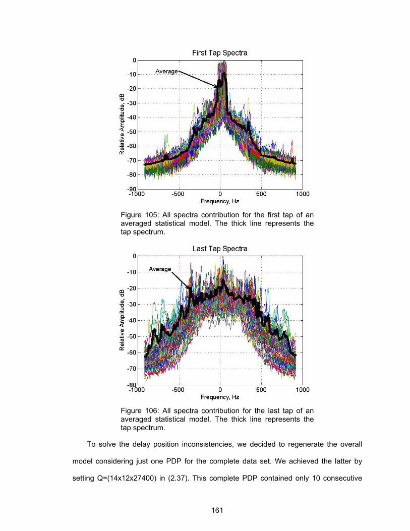
161

Figure 105: All spectra contribution for the first tap of an averaged statistical model. The thick line represents the tap spectrum.

Figure 106: All spectra contribution for the last tap of an averaged statistical model. The thick line represents the tap spectrum.

To solve the delay position inconsistencies, we decided to regenerate the overall

model considering just one PDP for the complete data set. We achieved the latter by

setting Q=(14x12x27400) in (2.37). This complete PDP contained only 10 consecutive

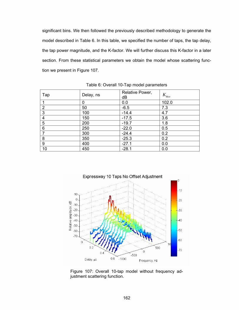
162

significant bins. We then followed the previously described methodology to generate the

model described in Table 6. In this table, we specified the number of taps, the tap delay,

the tap power magnitude, and the K-factor. We will further discuss this K-factor in a later

section. From these statistical parameters we obtain the model whose scattering func-

tion we present in Figure 107.

Table 6: Overall 10-Tap model parameters

Tap Delay, ns Relative Power, dB RiceK

1 0 0.0 102.0 2 50 -6.5 7.3 3 100 -14.4 4.7 4 150 -17.5 3.6 5 200 -19.7 1.8 6 250 -22.0 0.5 7 300 -24.4 0.2 8 350 -25.3 0.2 9 400 -27.1 0.0 10 450 -28.1 0.0

Figure 107: Overall 10-tap model without frequency ad-justment scattering function.

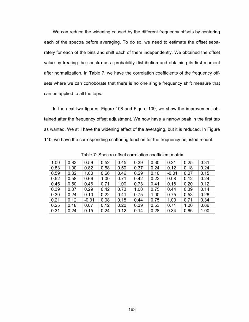
163

We can reduce the widening caused by the different frequency offsets by centering

each of the spectra before averaging. To do so, we need to estimate the offset sepa-

rately for each of the bins and shift each of them independently. We obtained the offset

value by treating the spectra as a probability distribution and obtaining its first moment

after normalization. In Table 7, we have the correlation coefficients of the frequency off-

sets where we can corroborate that there is no one single frequency shift measure that

can be applied to all the taps.

In the next two figures, Figure 108 and Figure 109, we show the improvement ob-

tained after the frequency offset adjustment. We now have a narrow peak in the first tap

as wanted. We still have the widening effect of the averaging, but it is reduced. In Figure

110, we have the corresponding scattering function for the frequency adjusted model.

Table 7: Spectra offset correlation coefficient matrix

1.00 0.83 0.59 0.52 0.45 0.39 0.30 0.21 0.25 0.31 0.83 1.00 0.82 0.58 0.50 0.37 0.24 0.12 0.18 0.24 0.59 0.82 1.00 0.66 0.46 0.29 0.10 -0.01 0.07 0.15 0.52 0.58 0.66 1.00 0.71 0.42 0.22 0.08 0.12 0.24 0.45 0.50 0.46 0.71 1.00 0.73 0.41 0.18 0.20 0.12 0.39 0.37 0.29 0.42 0.73 1.00 0.75 0.44 0.39 0.14 0.30 0.24 0.10 0.22 0.41 0.75 1.00 0.75 0.53 0.28 0.21 0.12 -0.01 0.08 0.18 0.44 0.75 1.00 0.71 0.34 0.25 0.18 0.07 0.12 0.20 0.39 0.53 0.71 1.00 0.66 0.31 0.24 0.15 0.24 0.12 0.14 0.28 0.34 0.66 1.00

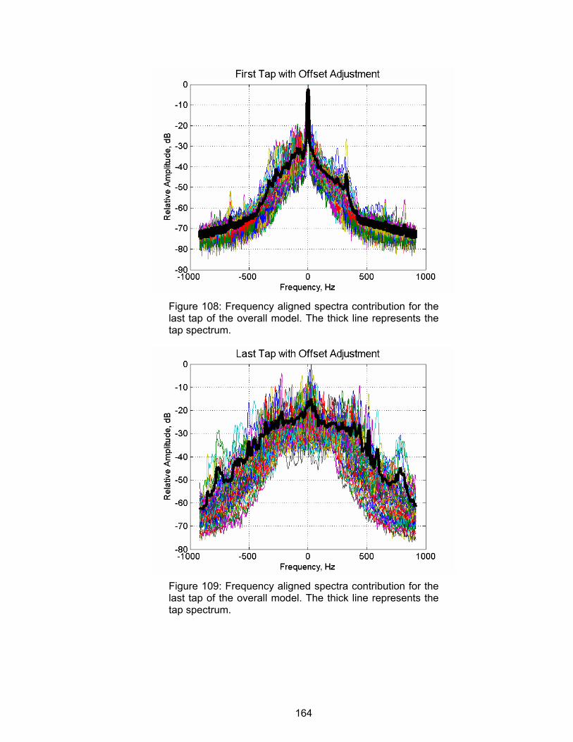
164

Figure 108: Frequency aligned spectra contribution for the last tap of the overall model. The thick line represents the tap spectrum.

Figure 109: Frequency aligned spectra contribution for the last tap of the overall model. The thick line represents the tap spectrum.

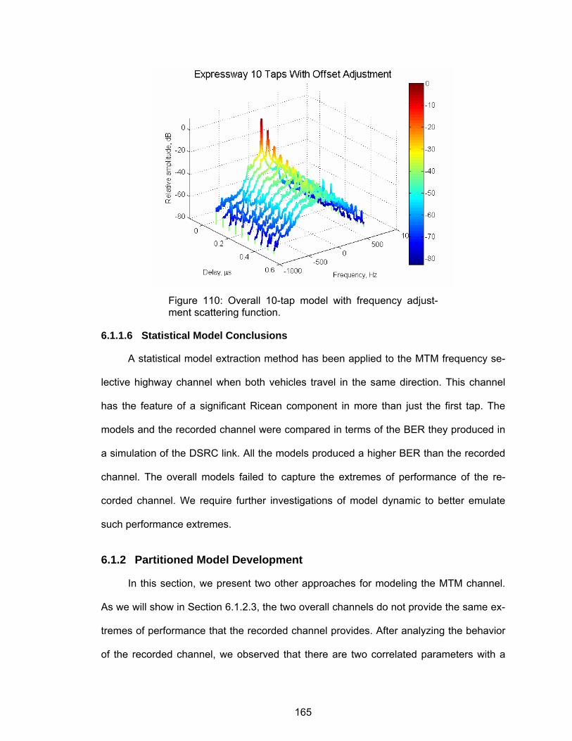
165

Figure 110: Overall 10-tap model with frequency adjust-ment scattering function.

6.1.1.6 Statistical Model Conclusions

A statistical model extraction method has been applied to the MTM frequency se-

lective highway channel when both vehicles travel in the same direction. This channel

has the feature of a significant Ricean component in more than just the first tap. The

models and the recorded channel were compared in terms of the BER they produced in

a simulation of the DSRC link. All the models produced a higher BER than the recorded

channel. The overall models failed to capture the extremes of performance of the re-

corded channel. We require further investigations of model dynamic to better emulate

such performance extremes.

6.1.2 Partitioned Model Development

In this section, we present two other approaches for modeling the MTM channel.

As we will show in Section 6.1.2.3, the two overall channels do not provide the same ex-

tremes of performance that the recorded channel provides. After analyzing the behavior

of the recorded channel, we observed that there are two correlated parameters with a

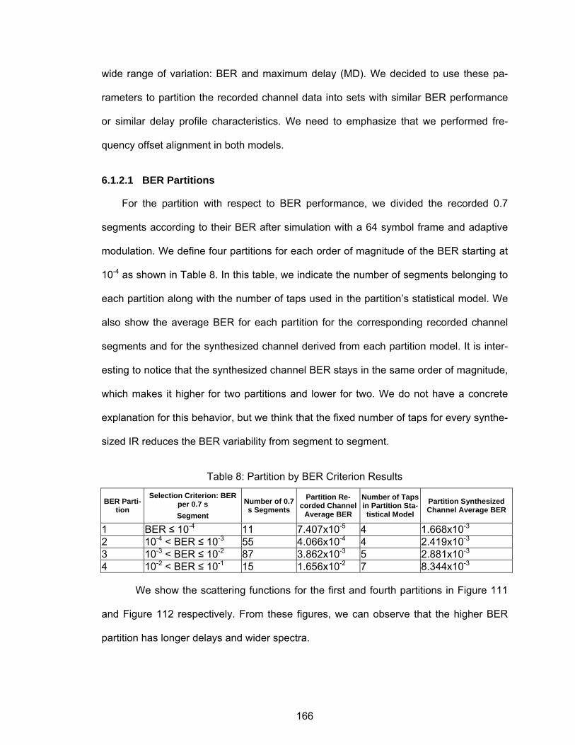
166

wide range of variation: BER and maximum delay (MD). We decided to use these pa-

rameters to partition the recorded channel data into sets with similar BER performance

or similar delay profile characteristics. We need to emphasize that we performed fre-

quency offset alignment in both models.

6.1.2.1 BER Partitions

For the partition with respect to BER performance, we divided the recorded 0.7

segments according to their BER after simulation with a 64 symbol frame and adaptive

modulation. We define four partitions for each order of magnitude of the BER starting at

10-4 as shown in Table 8. In this table, we indicate the number of segments belonging to

each partition along with the number of taps used in the partition’s statistical model. We

also show the average BER for each partition for the corresponding recorded channel

segments and for the synthesized channel derived from each partition model. It is inter-

esting to notice that the synthesized channel BER stays in the same order of magnitude,

which makes it higher for two partitions and lower for two. We do not have a concrete

explanation for this behavior, but we think that the fixed number of taps for every synthe-

sized IR reduces the BER variability from segment to segment.

Table 8: Partition by BER Criterion Results

BER Parti-tion

Selection Criterion: BER per 0.7 s Segment

Number of 0.7 s Segments

Partition Re-corded Channel

Average BER

Number of Taps in Partition Sta-tistical Model

Partition Synthesized Channel Average BER

1 BER ≤ 10-4 11 7.407x10-5 4 1.668x10-3 2 10-4 < BER ≤ 10-3 55 4.066x10-4 4 2.419x10-3 3 10-3 < BER ≤ 10-2 87 3.862x10-3 5 2.881x10-3 4 10-2 < BER ≤ 10-1 15 1.656x10-2 7 8.344x10-3

We show the scattering functions for the first and fourth partitions in Figure 111

and Figure 112 respectively. From these figures, we can observe that the higher BER

partition has longer delays and wider spectra.

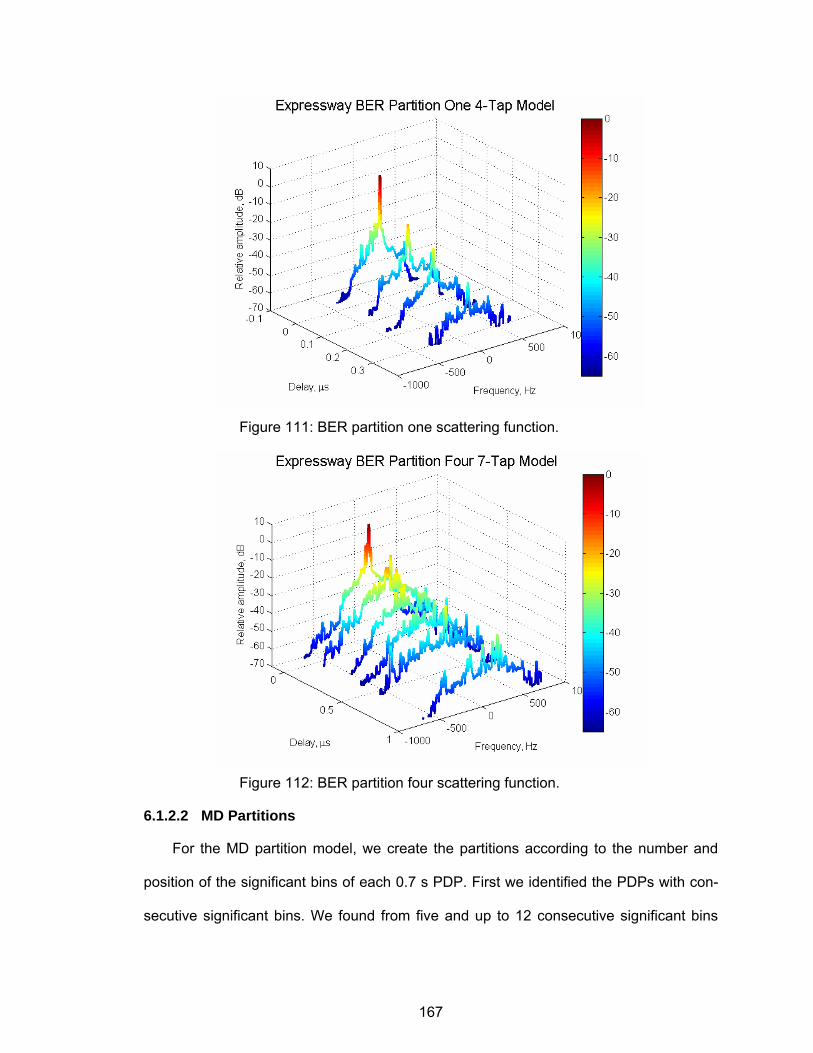
167

Figure 111: BER partition one scattering function.

Figure 112: BER partition four scattering function.

6.1.2.2 MD Partitions

For the MD partition model, we create the partitions according to the number and

position of the significant bins of each 0.7 s PDP. First we identified the PDPs with con-

secutive significant bins. We found from five and up to 12 consecutive significant bins

168

after the first. From this set, we created four partitions so that each partition model would

contain two consecutive bins per tap. For the non-consecutive significant bins, we cre-

ated two partitions: one for segments with less than 12 significant bins and one for seg-

ments with 12 or more significant bins. The number of segments per partitions is shown

in Table 9 where we also indicate the number of taps for the partition model. As in the

previous table, we also show the BER per partition for recorded and synthesized chan-

nels. Once again, we obtained BER of the same order of magnitude for the synthesized

channel.

Table 9: Partition by MD Results

Maximum Delay Parti-

tion

Selection Criterion: BER per 0.7 s Segment

Number of 0.7 s Seg-

ments

Partition Re-corded Channel

Average BER

Number of Taps in Partition Statistical

Model

Partition Synthe-sized Channel Aver-

age BER

1 5 & 6 Consecutive First Significant Bins 24 6.679x10-4 3 2.639x10-3




5 Long (>12) Non-consecutive Signifi-cant Bins

65 6.762x10-3 11 4.615x10-3

6 Short (<12) Non-consecutive Signifi-cant Bins

24 1.541x10-3 5 2.465x10-3

6.1.2.3 Results for Phase I Techniques

In this section, the models developed in the previous sections are compared in

terms of the CDF of the BER. The BER is impacted strongly by the length of the frame,

the length of the time period over which the BER is computed, and the choice of fixed or

adaptive modulation. Longer frames yield higher BER because the high initial quality of

the channel estimates degrades over time, even though there are pilot tones. The shape

of the CDF of the BER is impacted by the length of the observation interval because

169

zero and very low values of BER become less likely as the interval grows. Finally, the

type of modulation, fixed or adaptive, makes a difference, because ideally, adaptive

modulation makes the BER constant.

The BER will be computed for four cases, two which use adaptive modulation and

short frames, and two which use fixed modulation (6 Mbps) and long frames. The latter

case was included because it is the basis of the motion-related equipment test in the

current DSRC standard [6]. For adaptive modulation, two interval lengths are consid-

ered: 0.7 seconds, which corresponds to the “segment” length in the database, and 544

μs, which corresponds to a frame containing 64 symbols. For fixed modulation, the two

interval lengths are 0.7 seconds and 1.376 ms. The 1.376 ms frame holds 168 symbols,

or 1000 bytes of information at 6 Mbps; this is the “long frame” part of the motion-related

equipment test in the DSRC standard.

Figure 113 and Figure 114 contain the adaptive modulation results and Figures 19

and 20 contain the fixed modulation results. The adaptive modulation results include

CDFs of BER for the recorded channel and four models: the overall aligned, the overall

non-aligned, the BER partition, and the MD partition. Recall that for all models except

the overall non-aligned model, the segment spectra are centered prior to averaging. The

fixed modulation results include only the recorded channel and the BER partition model.

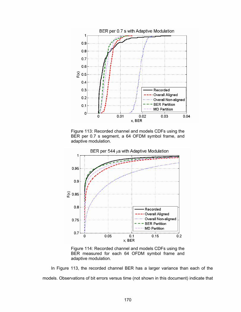
170

Figure 113: Recorded channel and models CDFs using the BER per 0.7 s segment, a 64 OFDM symbol frame, and adaptive modulation.

Figure 114: Recorded channel and models CDFs using the BER measured for each 64 OFDM symbol frame and adaptive modulation.

In Figure 113, the recorded channel BER has a larger variance than each of the

models. Observations of bit errors versus time (not shown in this document) indicate that

171

the recorded channel has relatively long periods of time when there are no errors, and

then other periods of time with a high density of bit errors. In contrast, the synthesized

channels produce a more uniform distribution of errors in time. Because the recorded

channel produces a significant percentage of 0.7 segments with zero or very few errors,

we may conclude that the low-error periods are often at least 0.7 seconds long.

In Figure 114, the BER partition model produces a very good fit to the recorded

channel. The MD partition model is next closest, and the overall aligned model is the

worst fit of the aligned models. Evidently, the 64 symbol frame is short enough that the

synthesized models produce between 80 and 90 percent error free frames.

As observed in Figure 115 and Figure 116, the long frames and fixed modulation

degrade the performance of the recorded channel and all the models. Interestingly, the

BER partition model and recorded channel diverge significantly for in the low BER region

when BER is computed over the long frame period (1.376 ms). Comparing Figure 114

and Figure 116, we observe that the BER partition model is only slightly degraded by the

longer frame and fixed modulation, but the recorded channel degrades significantly for

the longer frame. Long frame vs. short frame effects would seem to depend more on

small scale phenomena than large scale, and the long frame would suffer more from

Doppler spread. One possible reason for the divergence of these curves is that the de-

sign of the partition model was based on the short frame and adaptive modulation, yet in

Figure 116, the model is being evaluated on a link using a different type of modulation.

Had the partition model been based on the modulation assumed in Figure 116, fewer

segments would have been assigned to the lowest BER partition. The excessive number

of segments in the low BER partition could be the reason that the BER partition model

performs so much better than the recorded channel in the low BER regime.

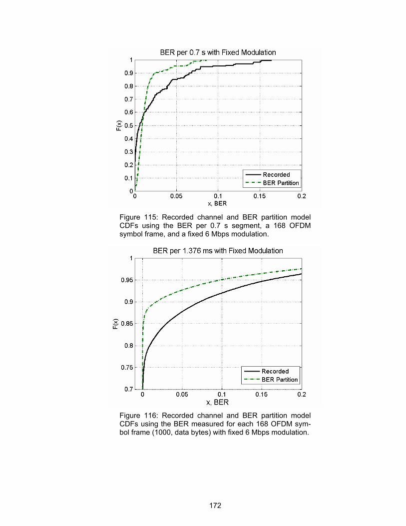
172

Figure 115: Recorded channel and BER partition model CDFs using the BER per 0.7 s segment, a 168 OFDM symbol frame, and a fixed 6 Mbps modulation.

Figure 116: Recorded channel and BER partition model CDFs using the BER measured for each 168 OFDM sym-bol frame (1000, data bytes) with fixed 6 Mbps modulation.

173

6.1.2.4 K-Factor

The Rice or K factor has not been part of our Phase One model specification, but it

is an important feature of models; therefore, it should be examined. Also, K-factors must

be explicitly specified in RF channel emulators. For these reasons, in this section, we

compute the K-factors of the taps of our models and compare them to the recorded

channel. We determine the Rice or K factor for any bin m using the moment-method [1],

[29] described in (2.40). Applying this method to each 0.7 s recorded segments, for

which Q = 27,400, we obtained a 168 x 511 K-factor matrix. Any complex K-factors were

set to zero. The K-factors given for the overall model in Table 10 are the first ten column

averages of the K-factor matrix. In Table 10, we present the K-factors for the corre-

sponding rows and columns of the K-factor matrix for each of the sections of the BER

partition model. For example, for Partition One; we have 11 0.7 s segments and seven

significant bins for the PDP of the partition. To obtain the K-factors for the partition, we

choose the corresponding rows and columns, and we perform a column average on the

new 11 x 7 matrix. For Table 10, we also calculated the K-factors for the synthesized

channel. Continuing with the partition one example, the partition contains four taps;

therefore, the K-factor submatrix size is 11 x 4. Each matrix element was obtained from

the 27,400 samples per tap of the synthesized channel. The table values are the column

averages.

By looking at the scattering function of Figure 111 and by considering the bins K-

factor values, we should expect a high K-factor for the first tap of the synthesized chan-

nel, but it is surprisingly small. This means that even when we use the recorded spectra,

which shows a significant K-factor, as the filter template for the synthesized channel, it is

not enough to create a representative K-factor. We have empirically notice that the seg-

ments with low BER present very high K-factors in the first bin, but we have also notice a

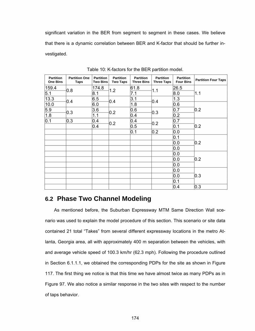
174

significant variation in the BER from segment to segment in these cases. We believe

that there is a dynamic correlation between BER and K-factor that should be further in-

vestigated.

Table 10: K-factors for the BER partition model.

Partition One Bins

Partition One Taps

Partition Two Bins

Partition Two Taps

Partition Three Bins

Partition Three Taps

Partition Four Bins Partition Four Taps

159.4 174.8 61.8 26.5 5.1 0.8 8.1 1.2 7.1 1.1 8.0 13.3 6.5 3.1 1.3

1.1

10.0 0.4 6.0 0.4 1.8 0.4 0.6 5.9 3.6 0.6 0.7 1.8 0.3 1.1 0.2 0.4 0.3 0.2

0.2

0.1 0.3 0.4 0.4 0.7 0.4 0.2 0.5 0.2 0.1 0.1 0.2 0.0

0.2

0.1 0.0 0.0

0.2

0.0 0.0 0.0

0.2

0.0 0.0 0.1

0.3

0.4 0.3

6.2 Phase Two Channel Modeling As mentioned before, the Suburban Expressway MTM Same Direction Wall sce-

nario was used to explain the model procedure of this section. This scenario or site data

contained 21 total “Takes” from several different expressway locations in the metro At-

lanta, Georgia area, all with approximately 400 m separation between the vehicles, with

and average vehicle speed of 100.3 km/hr (62.3 mph). Following the procedure outlined

in Section 6.1.1.1, we obtained the corresponding PDPs for the site as shown in Figure

117. The first thing we notice is that this time we have almost twice as many PDPs as in

Figure 97. We also notice a similar response in the two sites with respect to the number

of taps behavior.

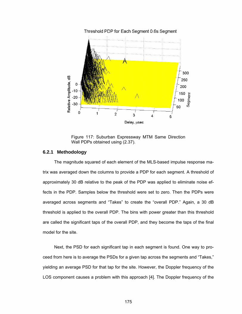
175

Figure 117: Suburban Expressway MTM Same Direction Wall PDPs obtained using (2.37).

6.2.1 Methodology

The magnitude squared of each element of the MLS-based impulse response ma-

trix was averaged down the columns to provide a PDP for each segment. A threshold of

approximately 30 dB relative to the peak of the PDP was applied to eliminate noise ef-

fects in the PDP. Samples below the threshold were set to zero. Then the PDPs were

averaged across segments and “Takes” to create the “overall PDP.” Again, a 30 dB

threshold is applied to the overall PDP. The bins with power greater than this threshold

are called the significant taps of the overall PDP, and they become the taps of the final

model for the site.

Next, the PSD for each significant tap in each segment is found. One way to pro-

ceed from here is to average the PSDs for a given tap across the segments and “Takes,”

yielding an average PSD for that tap for the site. However, the Doppler frequency of the

LOS component causes a problem with this approach [4]. The Doppler frequency of the

176

LOS component varies from segment to segment as the relative velocity of the vehicles

changes. Because of the changing Doppler of the LOS, the averaged spectrum ends up

having a broad peak which would not correspond to a Rician characteristic if that spec-

trum were used as a basis for channel simulation. In other words, a significant K factor is

indicated in a tap PSD by a spectral line. If a PSD without a narrow line is used as a ba-

sis for a filter in the filtered white noise approach to tap process simulation [37], then the

measured K factor for that simulated tap would be insignificant.

In Section 6.1.1.5, we dealt with this problem for the expressway same-direction

channel by aligning the spectra (i.e. translating them in frequency) before averaging,

such that the peaks of the aligned spectra were all at zero Doppler. Then we averaged

those spectra and ignored the somewhat less broad peak in our subjective shape-fitting

process. Since the same translation should not necessarily apply to all spectral compo-

nents, we decided to take a different and more objective approach in this modelling pro-

cedure.

For the procedure, we estimate the K factor of each bin in each segment using the

moment method [29], and we use this as a basis for removing the spectral peak. The K

factor is the ratio of the power of the “deterministic” or dominant spectral component

over the power of the random or diffuse reflection component. We note that the method

of moments approach measures the relative power of any phase or frequency modu-

lated component; it is not necessary that the component have zero Hz Doppler. Using

the K factor, we calculate the fraction of power that is attributed to the deterministic

component. By incrementally lowering a horizontal line, starting at the spectral peak, we

can identify the level such that the PSD area above this line equals the deterministic

power and the area below equals the random power. We then store the separated parts

of the spectrum and store the frequency of the peak for each segment. Finally, by aver-

177

aging the random parts across segments and “Takes,” we can arrive at an average ran-

dom spectral part for the site. We can also produce an average of the deterministic

parts, which shows the range of variation of the spectral line frequency and also shows

the influence of the segments with a particularly strong LOS. Alternatively, we can pro-

duce a histogram of spectral peak locations.

Our approach to identifying the shape of the random part of the spectrum is based

on the limitations of the RF channel emulators and by the type of link (OFDM) that is be-

ing evaluated. Usually, the identified channel model is intended to be an inherent prop-

erty of the channel, and applicable to any type of air interface with a similar RF fre-

quency and bandwidth. Therefore, propagation modellers are usually interested in the

geometrical properties of the channel, such as the distinct parameters of each path of

propagation, such as its power, delay and angle of arrival. However, our objective is only

to characterize the tap spectra, within the limited delay resolution of the target system

and the limited degrees of freedom of the RF channel emulator. The delay resolution

(100ns) of our measurements is large and corresponds to 30 m of excess path distance,

which will include many actual paths of propagation with different Doppler shifts. Fur-

thermore, for OFDM, if the excess delay is within the guard interval and if the channel

frequency response nulls are not too deep, then the primary channel impairment to the

link will be the ICI caused by the Doppler spreads of the tap processes [14]. This im-

pairment can be quantified based on the Doppler spectrum. Therefore, in our modelling

approach, we will attempt to optimally fit to the measured tap spectrum.

With such limited degrees of freedom in the fitting process, some parts of the spec-

trum will not be matched well. Therefore, the question arises, should certain parts of the

spectrum be considered as more important than others? For this, we will use a weighting

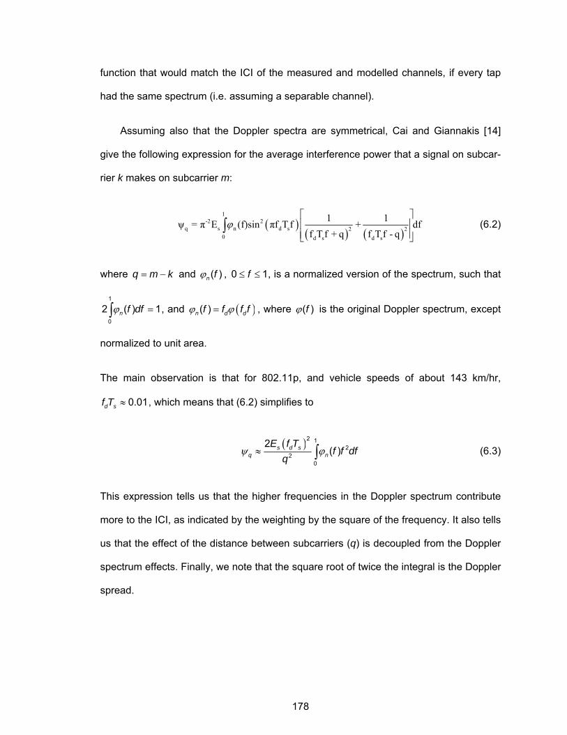
178

function that would match the ICI of the measured and modelled channels, if every tap

had the same spectrum (i.e. assuming a separable channel).

Assuming also that the Doppler spectra are symmetrical, Cai and Giannakis [14]

give the following expression for the average interference power that a signal on subcar-

rier k makes on subcarrier m:

( )( ) ( )

1-2 2

q s n d s 2 20 d s d s

1 1ψ = π E (f)sin πf T f + dff T f + q f T f - q

ϕ⎡ ⎤⎢ ⎥⎢ ⎥⎣ ⎦

∫ (6.2)

where = −q m k and ϕ ( )n f , ≤ ≤0 1f , is a normalized version of the spectrum, such that

ϕ =∫1

0

2 ( ) 1n f df , and ( )ϕ ϕ=( )n d df f f f , where ϕ( )f is the original Doppler spectrum, except

normalized to unit area.

The main observation is that for 802.11p, and vehicle speeds of about 143 km/hr,

≈ 0.01d sf T , which means that (6.2) simplifies to

( )ψ ϕ≈ ∫

2 12

20

2( )s d s

q n

E f Tf f df

q (6.3)

This expression tells us that the higher frequencies in the Doppler spectrum contribute

more to the ICI, as indicated by the weighting by the square of the frequency. It also tells

us that the effect of the distance between subcarriers (q) is decoupled from the Doppler

spectrum effects. Finally, we note that the square root of twice the integral is the Doppler

spread.

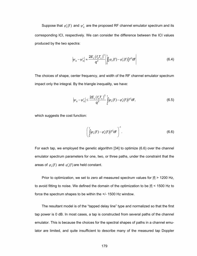
179

Suppose that ϕ′ ( )n f and ψ ′q are the proposed RF channel emulator spectrum and its

corresponding ICI, respectively. We can consider the difference between the ICI values

produced by the two spectra:

( ) [ ]ψ ψ ϕ ϕ′ ′− ≈ −∫2 1

22

0

2( ) ( )s d s

q q n n

E f Tf f f df

q (6.4)

The choices of shape, center frequency, and width of the RF channel emulator spectrum

impact only the integral. By the triangle inequality, we have:

( )ψ ψ ϕ ϕ′ ′− ≤ −∫

2 12

20

2( ) ( ) ,s d s

q q n n

E f Tf f f df

q (6.5)

which suggests the cost function:

ϕ ϕ−

⎛ ⎞′−⎜ ⎟

⎝ ⎠∫

112

0

( ) ( ) .n nf f f df (6.6)

For each tap, we employed the genetic algorithm [34] to optimize (6.6) over the channel

emulator spectrum parameters for one, two, or three paths, under the constraint that the

areas of ϕ ( )n f and ϕ′ ( )n f are held constant.

Prior to optimization, we set to zero all measured spectrum values for |f| > 1200 Hz,

to avoid fitting to noise. We defined the domain of the optimization to be |f| < 1500 Hz to

force the spectrum shapes to be within the +/- 1500 Hz window.

The resultant model is of the “tapped delay line” type and normalized so that the first

tap power is 0 dB. In most cases, a tap is constructed from several paths of the channel

emulator. This is because the choices for the spectral shapes of paths in a channel emu-

lator are limited, and quite insufficient to describe many of the measured tap Doppler

180

spectra. By superimposing several paths with nearly the same delay, it is possible to

create a customized Doppler spectrum that fits better. To avoid problems with the chan-

nel emulator, paths comprising a single tap were separated in delay by one nanosecond.

The customized Doppler spectrum is constrained to have the same total power (i.e.

same area in a non-dB plot) as the measured Doppler spectrum, so that the power delay

profile is preserved.

Each tap spectrum fit was optimized by taking the best of five runs of the genetic al-

gorithm. The cost function used in the genetic algorithm and for selecting the best of the

five was the integrated weighted difference between the measured spectrum and the

customized spectrum as indicated in (6.6). The weighting function was 2)( peakff − ,

where peakf is the frequency of the peak (usually very well defined) of the spectrum of

the first (and strongest) tap. It is assumed that peakf is the recovered carrier frequency in

the receiver. The cost function ensures that the ICI that would be produced by the cus-

tomized spectrum in an OFDM receiver is as close as possible to the ICI produced by

the measured spectrum [14]. In some cases, it seems that the fit of the customized spec-

trum to the measured spectrum could be made better by simply widening or shortening a

shape, however, this generally violates the equal power constraint.

6.2.2 Results for Phase II Techniques

In Figure 118, we show the overall PDP for the site. There are eight significant bins

or taps. In Figure 119, we have one snapshot of the Doppler spectrum for Tap One, illus-

trating the level method of Rician component removal. There is still a broad peak re-

maining, which may be there because of shifting of the Doppler frequency of the LOS

over the 0.6 s segment. In Figure 120, we present the histogram of Doppler frequencies

of the LOS for the 334 segments. The Doppler varies roughly from -100 Hz to +100 Hz.

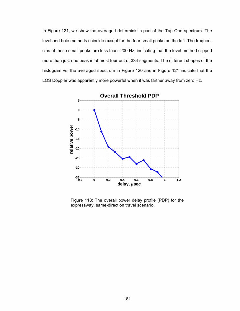
181

In Figure 121, we show the averaged deterministic part of the Tap One spectrum. The

level and hole methods coincide except for the four small peaks on the left. The frequen-

cies of these small peaks are less than -200 Hz, indicating that the level method clipped

more than just one peak in at most four out of 334 segments. The different shapes of the

histogram vs. the averaged spectrum in Figure 120 and in Figure 121 indicate that the

LOS Doppler was apparently more powerful when it was farther away from zero Hz.

Figure 118: The overall power delay profile (PDP) for the expressway, same-direction travel scenario.

-0.2 0 0.2 0.4 0.6 0.8 1 1.2-35

-30

-25

-20

-15

-10

-5

0

5Overall Threshold PDP

rela

tive

pow

er

delay, μsec

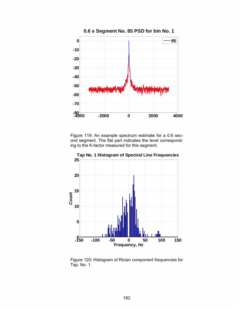
182

Figure 119: An example spectrum estimate for a 0.6 sec-ond segment. The flat part indicates the level correspond-ing to the K-factor measured for this segment.

Figure 120: Histogram of Rician component frequencies for Tap. No. 1.

-150 -100 -50 0 50 100 1500

5

10

15

20

25Tap No. 1 Histogram of Spectral Line Frequencies

Cou

nt

Frequency, Hz

-4000 -2000 0 2000 4000-80

-70

-60

-50

-40

-30

-20

-10

0

0.6 s Segment No. 85 PSD for bin No. 1

85

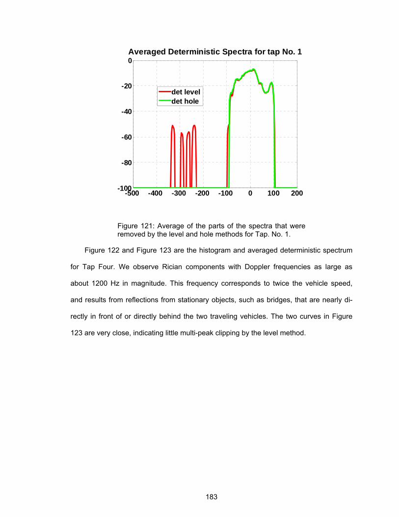
183

Figure 121: Average of the parts of the spectra that were removed by the level and hole methods for Tap. No. 1.

Figure 122 and Figure 123 are the histogram and averaged deterministic spectrum

for Tap Four. We observe Rician components with Doppler frequencies as large as

about 1200 Hz in magnitude. This frequency corresponds to twice the vehicle speed,

and results from reflections from stationary objects, such as bridges, that are nearly di-

rectly in front of or directly behind the two traveling vehicles. The two curves in Figure

123 are very close, indicating little multi-peak clipping by the level method.

-500 -400 -300 -200 -100 0 100 200-100

-80

-60

-40

-20

0Averaged Deterministic Spectra for tap No. 1

det leveldet hole

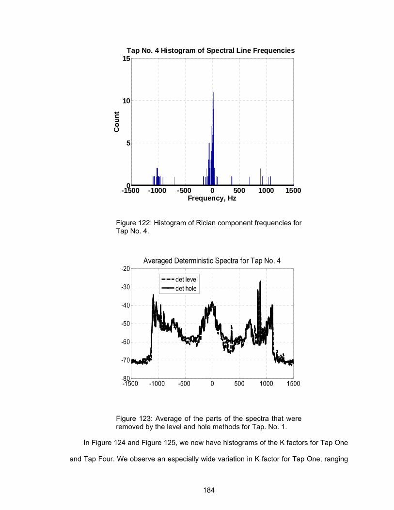
184

Figure 122: Histogram of Rician component frequencies for Tap No. 4.

-1500 -1000 -500 0 500 1000 1500-80

-70

-60

-50

-40

-30

-20Averaged Deterministic Spectra for Tap No. 4

det leveldet hole

Figure 123: Average of the parts of the spectra that were removed by the level and hole methods for Tap. No. 1.

In Figure 124 and Figure 125, we now have histograms of the K factors for Tap One

and Tap Four. We observe an especially wide variation in K factor for Tap One, ranging

-1500 -1000 -500 0 500 1000 15000

5

10

15Tap No. 4 Histogram of Spectral Line Frequencies

Cou

nt

Frequency, Hz

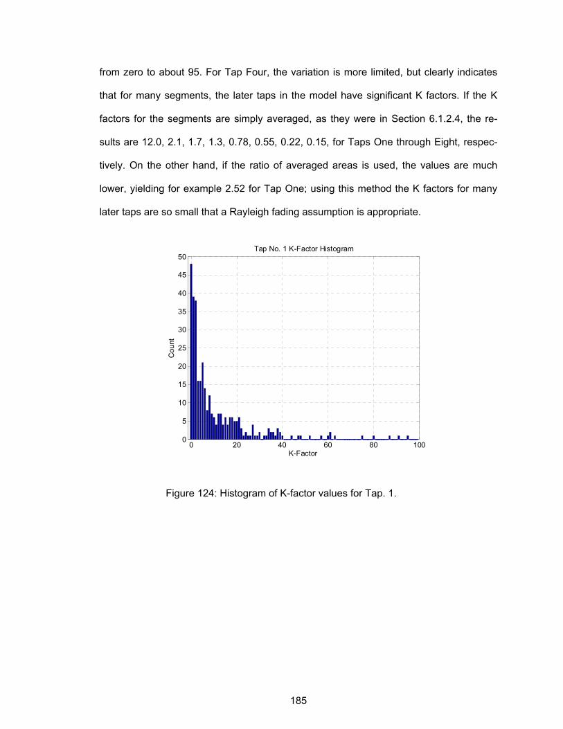
185

from zero to about 95. For Tap Four, the variation is more limited, but clearly indicates

that for many segments, the later taps in the model have significant K factors. If the K

factors for the segments are simply averaged, as they were in Section 6.1.2.4, the re-

sults are 12.0, 2.1, 1.7, 1.3, 0.78, 0.55, 0.22, 0.15, for Taps One through Eight, respec-

tively. On the other hand, if the ratio of averaged areas is used, the values are much

lower, yielding for example 2.52 for Tap One; using this method the K factors for many

later taps are so small that a Rayleigh fading assumption is appropriate.

0 20 40 60 80 1000

5

10

15

20

25

30

35

40

45

50Tap No. 1 K-Factor Histogram

Cou

nt

K-Factor

Figure 124: Histogram of K-factor values for Tap. 1.

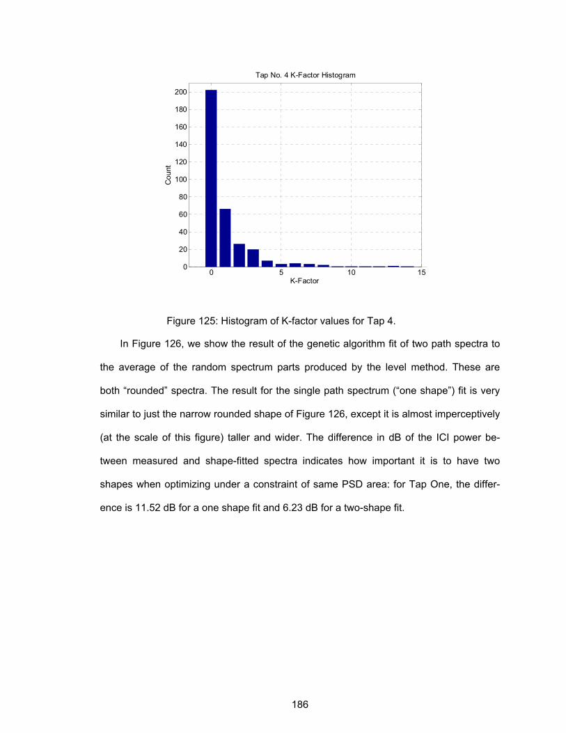
186

0 5 10 150

20

40

60

80

100

120

140

160

180

200

Tap No. 4 K-Factor Histogram

Cou

nt

K-Factor

Figure 125: Histogram of K-factor values for Tap 4.

In Figure 126, we show the result of the genetic algorithm fit of two path spectra to

the average of the random spectrum parts produced by the level method. These are

both “rounded” spectra. The result for the single path spectrum (“one shape”) fit is very

similar to just the narrow rounded shape of Figure 126, except it is almost imperceptively

(at the scale of this figure) taller and wider. The difference in dB of the ICI power be-

tween measured and shape-fitted spectra indicates how important it is to have two

shapes when optimizing under a constraint of same PSD area: for Tap One, the differ-

ence is 11.52 dB for a one shape fit and 6.23 dB for a two-shape fit.

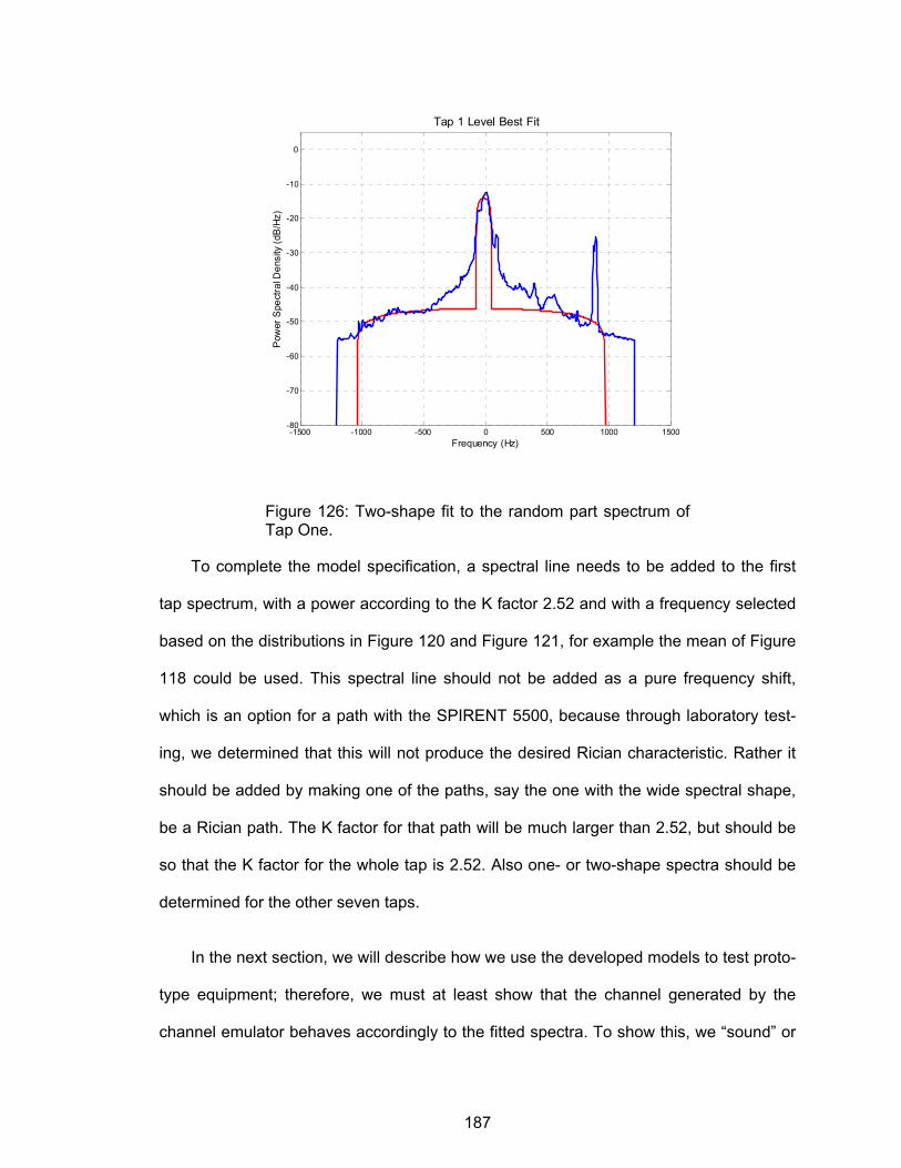
187

-1500 -1000 -500 0 500 1000 1500-80

-70

-60

-50

-40

-30

-20

-10

0

Tap 1 Level Best Fit

Pow

er S

pect

ral D

ensi

ty (d

B/H

z)

Frequency (Hz)

Figure 126: Two-shape fit to the random part spectrum of Tap One.

To complete the model specification, a spectral line needs to be added to the first

tap spectrum, with a power according to the K factor 2.52 and with a frequency selected

based on the distributions in Figure 120 and Figure 121, for example the mean of Figure

118 could be used. This spectral line should not be added as a pure frequency shift,

which is an option for a path with the SPIRENT 5500, because through laboratory test-

ing, we determined that this will not produce the desired Rician characteristic. Rather it

should be added by making one of the paths, say the one with the wide spectral shape,

be a Rician path. The K factor for that path will be much larger than 2.52, but should be

so that the K factor for the whole tap is 2.52. Also one- or two-shape spectra should be

determined for the other seven taps.

In the next section, we will describe how we use the developed models to test proto-

type equipment; therefore, we must at least show that the channel generated by the

channel emulator behaves accordingly to the fitted spectra. To show this, we “sound” or

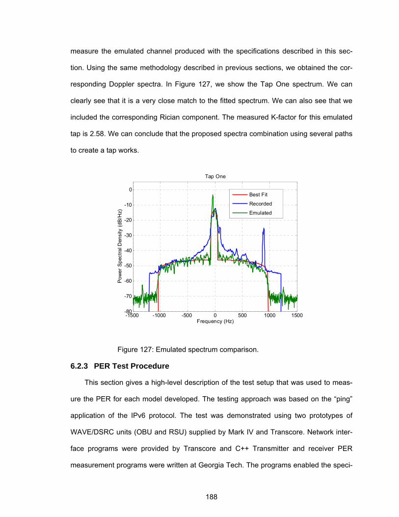
188

measure the emulated channel produced with the specifications described in this sec-

tion. Using the same methodology described in previous sections, we obtained the cor-

responding Doppler spectra. In Figure 127, we show the Tap One spectrum. We can

clearly see that it is a very close match to the fitted spectrum. We can also see that we

included the corresponding Rician component. The measured K-factor for this emulated

tap is 2.58. We can conclude that the proposed spectra combination using several paths

to create a tap works.

-1500 -1000 -500 0 500 1000 1500-80

-70

-60

-50

-40

-30

-20

-10

0

Tap One

Pow

er S

pect

ral D

ensi

ty (d

B/H

z)

Frequency (Hz)

Best Fit

Recorded

Emulated

Figure 127: Emulated spectrum comparison.

6.2.3 PER Test Procedure

This section gives a high-level description of the test setup that was used to meas-

ure the PER for each model developed. The testing approach was based on the “ping”

application of the IPv6 protocol. The test was demonstrated using two prototypes of

WAVE/DSRC units (OBU and RSU) supplied by Mark IV and Transcore. Network inter-

face programs were provided by Transcore and C++ Transmitter and receiver PER

measurement programs were written at Georgia Tech. The programs enabled the speci-

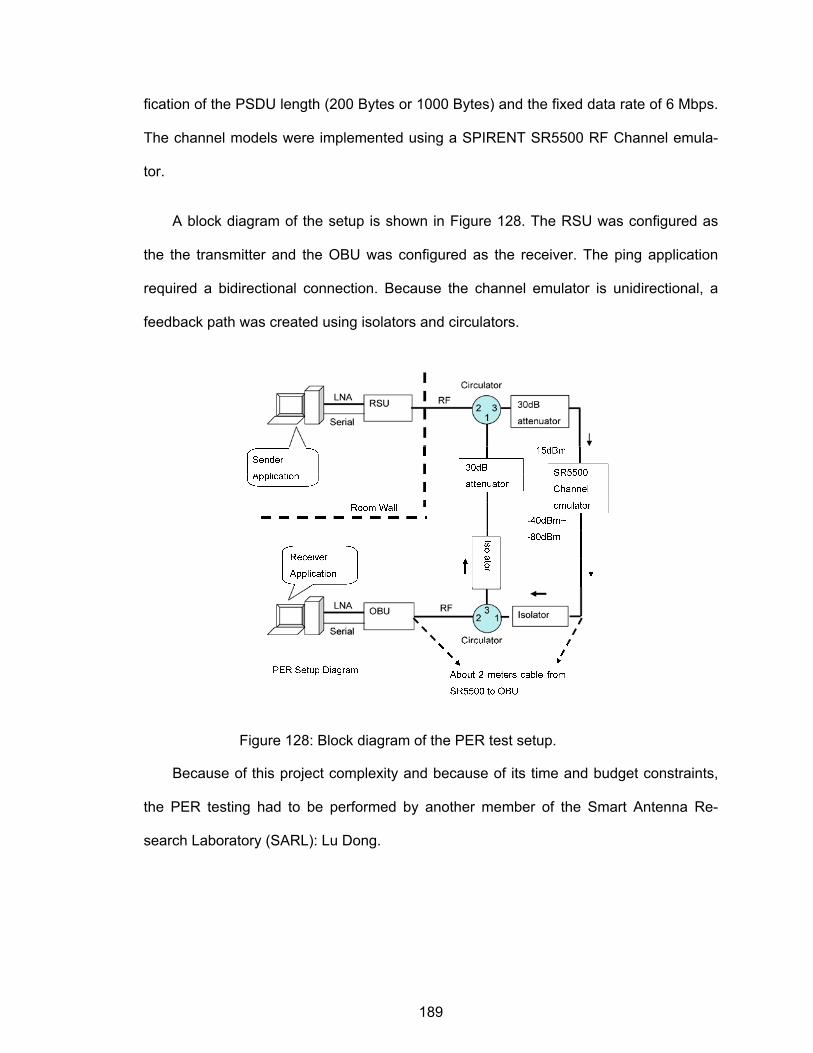
189

fication of the PSDU length (200 Bytes or 1000 Bytes) and the fixed data rate of 6 Mbps.

The channel models were implemented using a SPIRENT SR5500 RF Channel emula-

tor.

A block diagram of the setup is shown in Figure 128. The RSU was configured as

the the transmitter and the OBU was configured as the receiver. The ping application

required a bidirectional connection. Because the channel emulator is unidirectional, a

feedback path was created using isolators and circulators.

Figure 128: Block diagram of the PER test setup.

Because of this project complexity and because of its time and budget constraints,

the PER testing had to be performed by another member of the Smart Antenna Re-

search Laboratory (SARL): Lu Dong.

190

6.2.4 Phase II Model Conclusions

We have described an approach to channel identification for the purpose of RF

channel emulation or Simulink simulation for the MTM channel in the expressway, same-

direction travel scenario. Because of limited degrees of freedom in spectrum fitting, we

used weighting function to ensure that the ICI for OFDM that is produced by the model

tap is as near as possible to that of the measured channel, given a constraint on tap

power. With this weighting function, it is clear that at least two shapes per tap are neces-

sary to model the first tap of the model.

The histograms of K factors shown for Phase Two have a wide range of variation,

even in later taps. However, since for most of the segments, the K factors are low, then

the K factors based on average powers are low, and can be approximated as zero for all

taps but the first.

The most important lesson we have learned trough the model development for

Phase Two is that the fixed K-factor produced in channel emulation or simulation does

not represent the real behavior of the MTM channel; therefore, in order to properly de-

scribe this type of communication channel, it is necessary to include the dynamic char-

acteristics of the K-factor.

191

CHAPTER 7

MODEL SUMMARIES

7.1 Proposed WAVE/DSRC Model As we mentioned in Section 5.2, the purpose of this investigation has been to define

the model to be used in the motion-related equipment certification test for the standard.

The model we recommend for the test is the MTM Expressway Oncoming without Wall,

because it produces the highest PER among all the channels for the prototype

WAVE/DSRC transceivers that were provided to Georgia Tech.

The models represent six of the environments in which the WAVE/DSRC system is

expected to operate; three of them are for the MTM link, and the other three are for the

RTM link. The models are listed below in order of the PER (from results indicated by Lu

Dong) they produced for 1000 Byte packets, from highest (worst channel) to lowest (best

channel).

1. MTM – Expressway Oncoming Without Wall, 300m – 400m

2. RTM – Urban Canyon, 100m

3. RTM – Expressway, 300m – 400m

4. MTM – Urban Canyon Oncoming, 100m

5. RTM – Suburban Street, 100m

6. MTM – Expressway Same Direction with Wall, 300m – 400m

The small-scale fading models represent multipath fading effects only and do not in-

clude path loss or lognormal shadowing.

192

7.2 Model Descriptions In some cases, two models, “long” and “short,” are presented. The short models use

a maximum of 12 paths, which is the maximum number of paths on many RF channel

emulators. Some channel emulators, such as the model SR5500, have 24 paths, so they

can run the “long” model, which has more than 12 paths. When given, the long model

has a better fit to the measured spectrum. PER results are presented for both long and

short models, so that the user can see how much they differ in terms of PER.

The parameters are named according to the Spirent SR5500 TestKit Instrument

Control Software [Section 2.3], [79]. For example, “Fading Spectral Shape” is the Dop-

pler spectrum shape, “Frequency Shift” is the center frequency of the path’s fading spec-

tral shape, and “Fading Doppler” is the half-width of the path’s fading spectral shape.

“n/a” means “not applicable.”

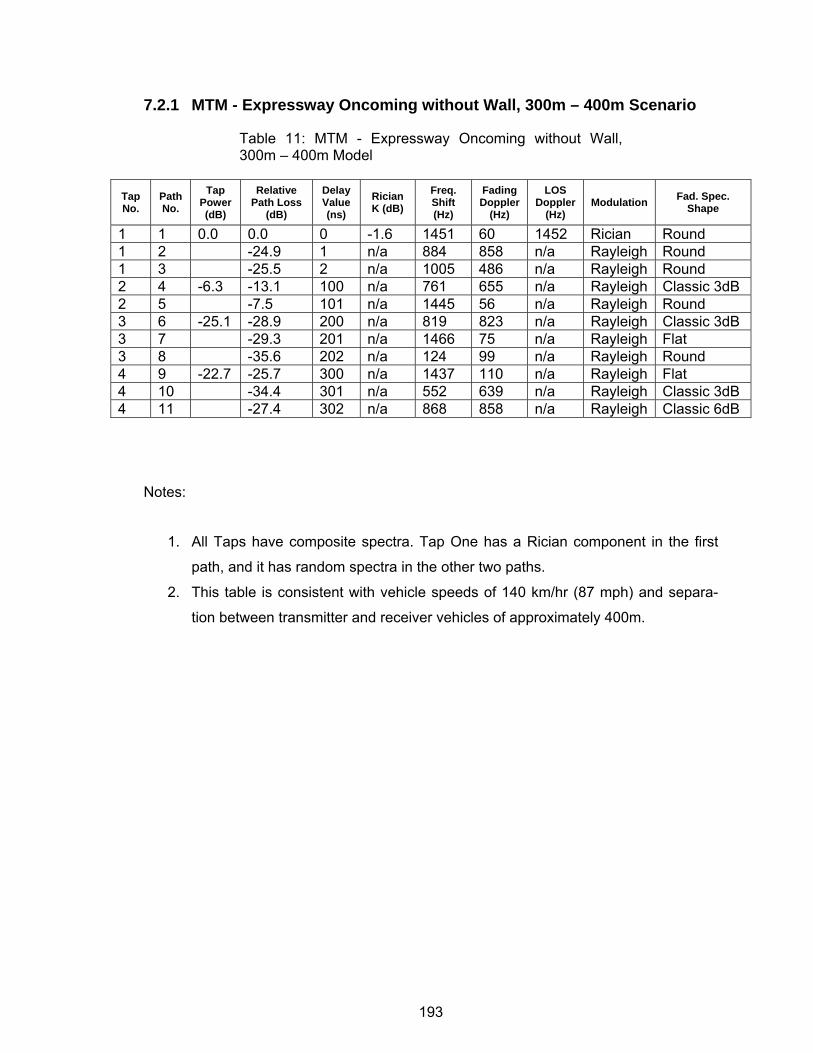
193

7.2.1 MTM - Expressway Oncoming without Wall, 300m – 400m Scenario

Table 11: MTM - Expressway Oncoming without Wall, 300m – 400m Model

Tap No.

Path No.

Tap Power (dB)

Relative Path Loss

(dB)

Delay Value (ns)

Rician K (dB)

Freq. Shift (Hz)

Fading Doppler

(Hz)

LOS Doppler

(Hz) Modulation Fad. Spec.

Shape

1 1 0.0 0.0 0 -1.6 1451 60 1452 Rician Round 1 2 -24.9 1 n/a 884 858 n/a Rayleigh Round 1 3 -25.5 2 n/a 1005 486 n/a Rayleigh Round 2 4 -6.3 -13.1 100 n/a 761 655 n/a Rayleigh Classic 3dB 2 5 -7.5 101 n/a 1445 56 n/a Rayleigh Round 3 6 -25.1 -28.9 200 n/a 819 823 n/a Rayleigh Classic 3dB 3 7 -29.3 201 n/a 1466 75 n/a Rayleigh Flat 3 8 -35.6 202 n/a 124 99 n/a Rayleigh Round 4 9 -22.7 -25.7 300 n/a 1437 110 n/a Rayleigh Flat 4 10 -34.4 301 n/a 552 639 n/a Rayleigh Classic 3dB 4 11 -27.4 302 n/a 868 858 n/a Rayleigh Classic 6dB

Notes:

1. All Taps have composite spectra. Tap One has a Rician component in the first

path, and it has random spectra in the other two paths.

2. This table is consistent with vehicle speeds of 140 km/hr (87 mph) and separa-

tion between transmitter and receiver vehicles of approximately 400m.

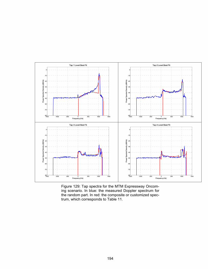
194

-1500 -1000 -500 0 500 1000 1500-80

-70

-60

-50

-40

-30

-20

-10

0


Pow

er S

pect

ral D

ensi

ty (d

B/H

z)

Frequency (Hz)-1500 -1000 -500 0 500 1000 1500

-80

-70

-60

-50

-40

-30

-20

-10

0


Pow

er S

pect

ral D

ensi

ty (d

B/H

z)

Frequency (Hz)

-1500 -1000 -500 0 500 1000 1500-80

-70

-60

-50

-40

-30

-20

-10

0


Pow

er S

pect

ral D

ensi

ty (d

B/H

z)

Frequency (Hz)-1500 -1000 -500 0 500 1000 1500

-80

-70

-60

-50

-40

-30

-20

-10

0

Tap 4 Level Best FitP

ower

Spe

ctra

l Den

sity

(dB

/Hz)

Frequency (Hz)

Figure 129: Tap spectra for the MTM Expressway Oncom-ing scenario. In blue: the measured Doppler spectrum for the random part. In red: the composite or customized spec-trum, which corresponds to Table 11.

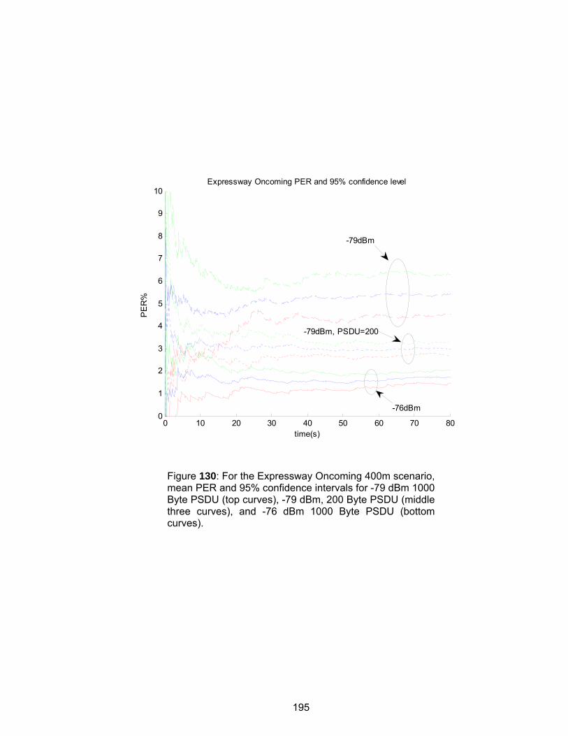
195

0 10 20 30 40 50 60 70 800

1

2

3

4

5

6

7

8

9

10

time(s)

PE

R%

Expressway Oncoming PER and 95% confidence level

-76dBm

-79dBm

-79dBm, PSDU=200

Figure 130: For the Expressway Oncoming 400m scenario, mean PER and 95% confidence intervals for -79 dBm 1000 Byte PSDU (top curves), -79 dBm, 200 Byte PSDU (middle three curves), and -76 dBm 1000 Byte PSDU (bottom curves).

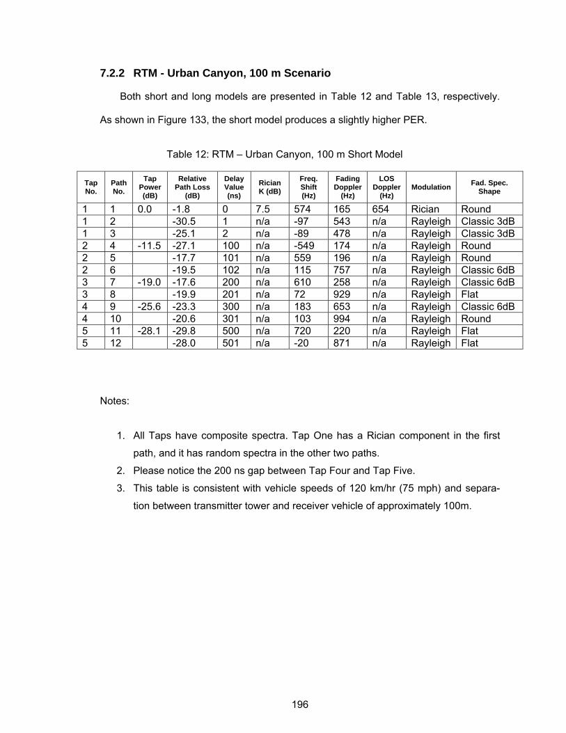
196

7.2.2 RTM - Urban Canyon, 100 m Scenario

Both short and long models are presented in Table 12 and Table 13, respectively.

As shown in Figure 133, the short model produces a slightly higher PER.

Table 12: RTM – Urban Canyon, 100 m Short Model

Tap No.

Path No.

Tap Power (dB)

Relative Path Loss

(dB)

Delay Value (ns)

Rician K (dB)

Freq. Shift (Hz)

Fading Doppler

(Hz)

LOS Doppler


Shape

1 1 0.0 -1.8 0 7.5 574 165 654 Rician Round 1 2 -30.5 1 n/a -97 543 n/a Rayleigh Classic 3dB 1 3 -25.1 2 n/a -89 478 n/a Rayleigh Classic 3dB 2 4 -11.5 -27.1 100 n/a -549 174 n/a Rayleigh Round 2 5 -17.7 101 n/a 559 196 n/a Rayleigh Round 2 6 -19.5 102 n/a 115 757 n/a Rayleigh Classic 6dB 3 7 -19.0 -17.6 200 n/a 610 258 n/a Rayleigh Classic 6dB 3 8 -19.9 201 n/a 72 929 n/a Rayleigh Flat 4 9 -25.6 -23.3 300 n/a 183 653 n/a Rayleigh Classic 6dB 4 10 -20.6 301 n/a 103 994 n/a Rayleigh Round 5 11 -28.1 -29.8 500 n/a 720 220 n/a Rayleigh Flat 5 12 -28.0 501 n/a -20 871 n/a Rayleigh Flat

Notes:



2. Please notice the 200 ns gap between Tap Four and Tap Five.


tion between transmitter tower and receiver vehicle of approximately 100m.

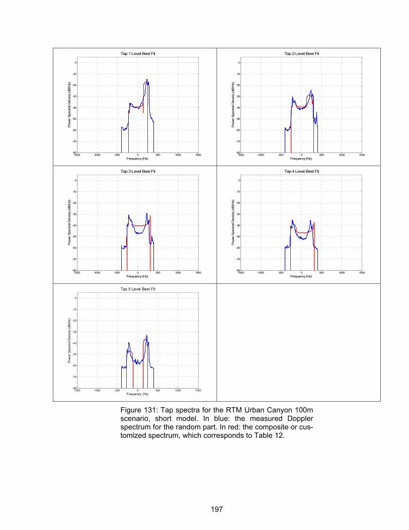
197

-1500 -1000 -500 0 500 1000 1500-80

-70

-60

-50

-40

-30

-20

-10

0


Pow

er S

pect

ral D

ensi

ty (d

B/H

z)

Frequency (Hz)-1500 -1000 -500 0 500 1000 1500

-80

-70

-60

-50

-40

-30

-20

-10

0


Pow

er S

pect

ral D

ensi

ty (d

B/H

z)

Frequency (Hz)

-1500 -1000 -500 0 500 1000 1500-80

-70

-60

-50

-40

-30

-20

-10

0


Pow

er S

pect

ral D

ensi

ty (d

B/H

z)

Frequency (Hz)-1500 -1000 -500 0 500 1000 1500

-80

-70

-60

-50

-40

-30

-20

-10

0


Pow

er S

pect

ral D

ensi

ty (d

B/H

z)

Frequency (Hz)

-1500 -1000 -500 0 500 1000 1500-80

-70

-60

-50

-40

-30

-20

-10

0


Pow

er S

pect

ral D

ensi

ty (d

B/H

z)

Frequency (Hz)

Figure 131: Tap spectra for the RTM Urban Canyon 100m scenario, short model. In blue: the measured Doppler spectrum for the random part. In red: the composite or cus-tomized spectrum, which corresponds to Table 12.

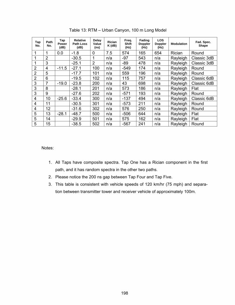
198

Table 13: RTM – Urban Canyon, 100 m Long Model

Tap No.

Path No.

Tap Power (dB)

Relative Path Loss

(dB)

Delay Value (ns)

Rician K (dB)

Freq. Shift (Hz)

Fading Doppler

(Hz)

LOS Doppler


Shape

1 1 0.0 -1.8 0 7.5 574 165 654 Rician Round 1 2 -30.5 1 n/a -97 543 n/a Rayleigh Classic 3dB 1 3 -25.1 2 n/a -89 478 n/a Rayleigh Classic 3dB 2 4 -11.5 -27.1 100 n/a -549 174 n/a Rayleigh Round 2 5 -17.7 101 n/a 559 196 n/a Rayleigh Round 2 6 -19.5 102 n/a 115 757 n/a Rayleigh Classic 6dB 3 7 -19.0 -23.8 200 n/a 43 698 n/a Rayleigh Classic 6dB 3 8 -28.1 201 n/a 573 186 n/a Rayleigh Flat 3 9 -27.6 202 n/a -571 193 n/a Rayleigh Round 4 10 -25.6 -33.4 300 n/a -137 494 n/a Rayleigh Classic 6dB 4 11 -30.5 301 n/a -573 211 n/a Rayleigh Round 4 12 -31.6 302 n/a 576 250 n/a Rayleigh Round 5 13 -28.1 -48.7 500 n/a -506 644 n/a Rayleigh Flat 5 14 -29.9 501 n/a 575 162 n/a Rayleigh Flat 5 15 -38.5 502 n/a -567 241 n/a Rayleigh Round

Notes:



2. Please notice the 200 ns gap between Tap Four and Tap Five.



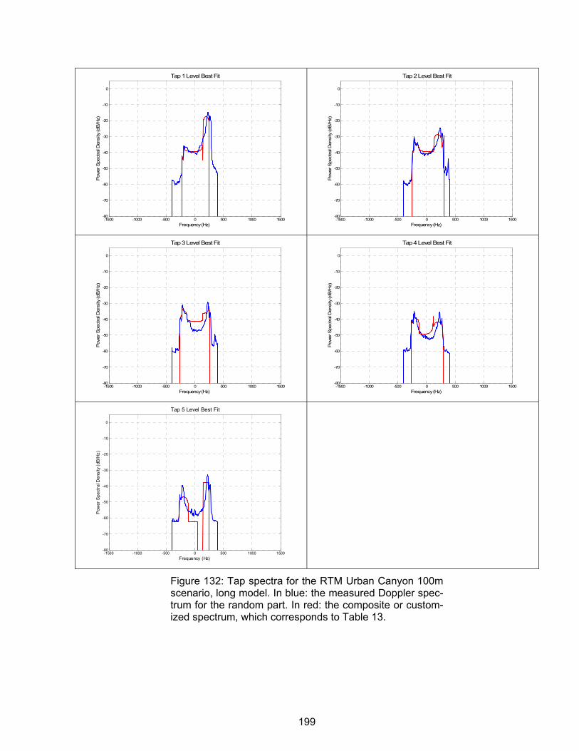
199

-1500 -1000 -500 0 500 1000 1500-80

-70

-60

-50

-40

-30

-20

-10

0


Pow

er S

pect

ral D

ensi

ty (d

B/H

z)

Frequency (Hz)-1500 -1000 -500 0 500 1000 1500

-80

-70

-60

-50

-40

-30

-20

-10

0


Pow

er S

pect

ral D

ensi

ty (d

B/H

z)

Frequency (Hz)

-1500 -1000 -500 0 500 1000 1500-80

-70

-60

-50

-40

-30

-20

-10

0


Pow

er S

pect

ral D

ensi

ty (d

B/H

z)

Frequency (Hz)-1500 -1000 -500 0 500 1000 1500

-80

-70

-60

-50

-40

-30

-20

-10

0


Pow

er S

pect

ral D

ensi

ty (d

B/H

z)

Frequency (Hz)

-1500 -1000 -500 0 500 1000 1500-80

-70

-60

-50

-40

-30

-20

-10

0


Pow

er S

pect

ral D

ensi

ty (d

B/H

z)

Frequency (Hz)

Figure 132: Tap spectra for the RTM Urban Canyon 100m scenario, long model. In blue: the measured Doppler spec-trum for the random part. In red: the composite or custom-ized spectrum, which corresponds to Table 13.

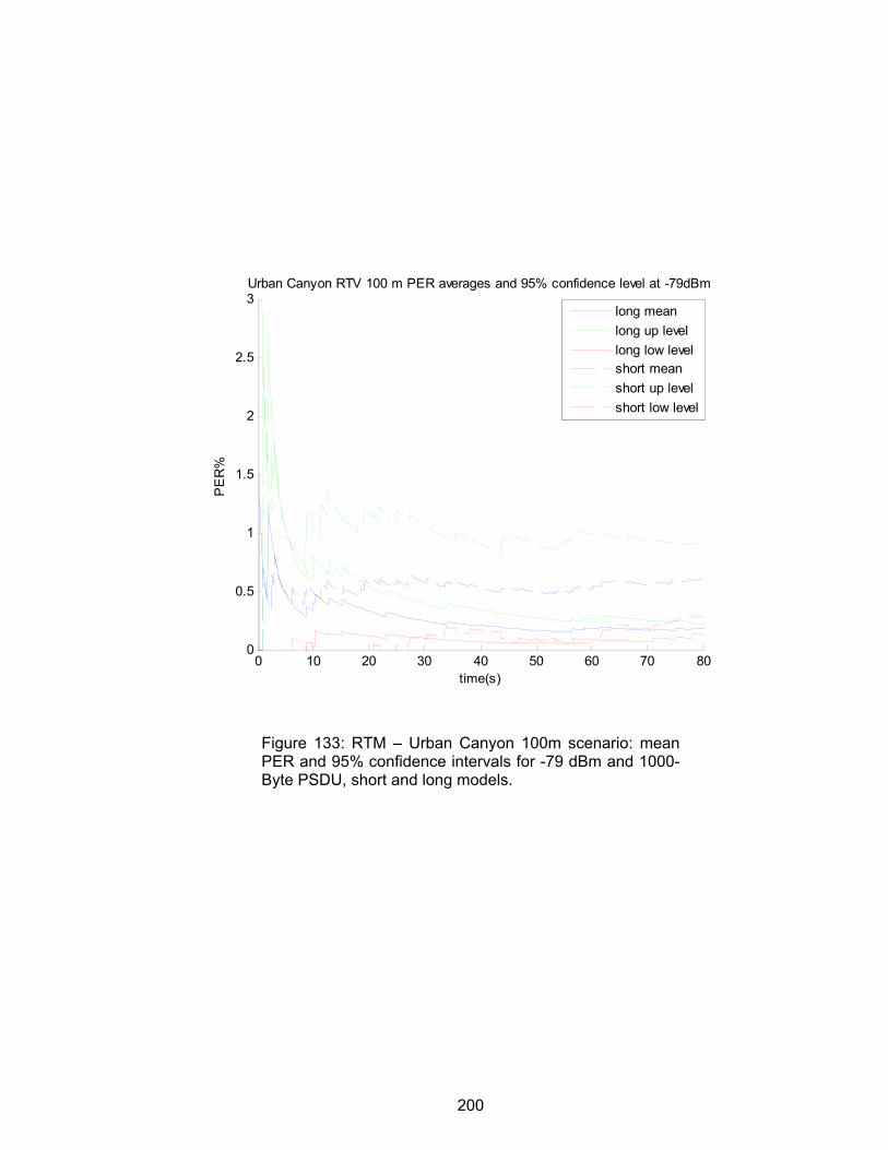
200

0 10 20 30 40 50 60 70 800

0.5

1

1.5

2

2.5

3

time(s)

PE

R%

Urban Canyon RTV 100 m PER averages and 95% confidence level at -79dBm

long meanlong up levellong low levelshort meanshort up levelshort low level

Figure 133: RTM – Urban Canyon 100m scenario: mean PER and 95% confidence intervals for -79 dBm and 1000-Byte PSDU, short and long models.

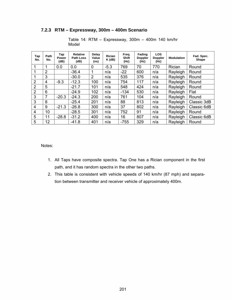
201

7.2.3 RTM – Expressway, 300m – 400m Scenario

Table 14: RTM – Expressway, 300m – 400m 140 km/hr Model

Tap No.

Path No.

Tap Power (dB)

Relative Path Loss

(dB)

Delay Value (ns)

Rician K (dB)

Freq. Shift (Hz)

Fading Doppler

(Hz)

LOS Doppler


Shape

1 1 0.0 0.0 0 -5.3 769 70 770 Rician Round 1 2 -36.4 1 n/a -22 600 n/a Rayleigh Round 1 3 -30.0 2 n/a 535 376 n/a Rayleigh Round 2 4 -9.3 -12.3 100 n/a 754 117 n/a Rayleigh Round 2 5 -21.7 101 n/a 548 424 n/a Rayleigh Round 2 6 -24.9 102 n/a -134 530 n/a Rayleigh Flat 3 7 -20.3 -24.3 200 n/a 761 104 n/a Rayleigh Round 3 8 -25.4 201 n/a 88 813 n/a Rayleigh Classic 3dB 4 9 -21.3 -26.8 300 n/a 37 802 n/a Rayleigh Classic 6dB 4 10 -28.5 301 n/a 752 91 n/a Rayleigh Round 5 11 -28.8 -31.2 400 n/a 16 807 n/a Rayleigh Classic 6dB 5 12 -41.8 401 n/a -755 329 n/a Rayleigh Round

Notes:




tion between transmitter and receiver vehicle of approximately 400m.

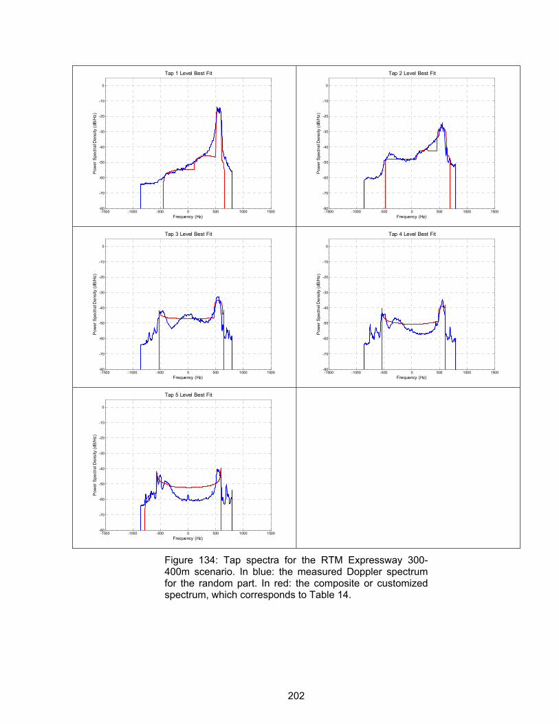
202

-1500 -1000 -500 0 500 1000 1500-80

-70

-60

-50

-40

-30

-20

-10

0


Pow

er S

pect

ral D

ensi

ty (d

B/H

z)

Frequency (Hz)-1500 -1000 -500 0 500 1000 1500

-80

-70

-60

-50

-40

-30

-20

-10

0


Pow

er S

pect

ral D

ensi

ty (d

B/H

z)

Frequency (Hz)

-1500 -1000 -500 0 500 1000 1500-80

-70

-60

-50

-40

-30

-20

-10

0


Pow

er S

pect

ral D

ensi

ty (d

B/H

z)

Frequency (Hz)-1500 -1000 -500 0 500 1000 1500

-80

-70

-60

-50

-40

-30

-20

-10

0


Pow

er S

pect

ral D

ensi

ty (d

B/H

z)

Frequency (Hz)

-1500 -1000 -500 0 500 1000 1500-80

-70

-60

-50

-40

-30

-20

-10

0


Pow

er S

pect

ral D

ensi

ty (d

B/H

z)

Frequency (Hz)

Figure 134: Tap spectra for the RTM Expressway 300-400m scenario. In blue: the measured Doppler spectrum for the random part. In red: the composite or customized spectrum, which corresponds to Table 14.

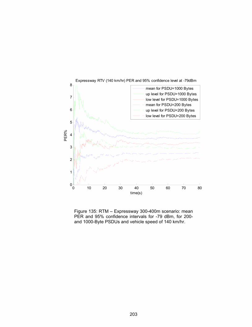
203

0 10 20 30 40 50 60 70 800

1

2

3

4

5

6

7

8

time(s)

PE

R%

Expressway RTV (140 km/hr) PER and 95% confidence level at -79dBm

mean for PSDU=1000 Bytesup level for PSDU=1000 Byteslow level for PSDU=1000 Bytesmean for PSDU=200 Bytesup level for PSDU=200 Byteslow level for PSDU=200 Bytes

Figure 135: RTM – Expressway 300-400m scenario: mean PER and 95% confidence intervals for -79 dBm, for 200- and 1000-Byte PSDUs and vehicle speed of 140 km/hr.

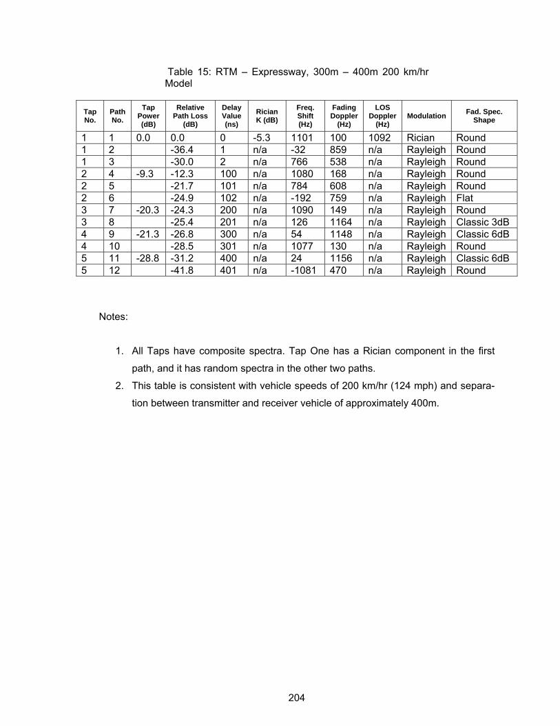
204

Table 15: RTM – Expressway, 300m – 400m 200 km/hr Model

Tap No.

Path No.

Tap Power (dB)

Relative Path Loss

(dB)

Delay Value (ns)

Rician K (dB)

Freq. Shift (Hz)

Fading Doppler

(Hz)

LOS Doppler


Shape

1 1 0.0 0.0 0 -5.3 1101 100 1092 Rician Round 1 2 -36.4 1 n/a -32 859 n/a Rayleigh Round 1 3 -30.0 2 n/a 766 538 n/a Rayleigh Round 2 4 -9.3 -12.3 100 n/a 1080 168 n/a Rayleigh Round 2 5 -21.7 101 n/a 784 608 n/a Rayleigh Round 2 6 -24.9 102 n/a -192 759 n/a Rayleigh Flat 3 7 -20.3 -24.3 200 n/a 1090 149 n/a Rayleigh Round 3 8 -25.4 201 n/a 126 1164 n/a Rayleigh Classic 3dB 4 9 -21.3 -26.8 300 n/a 54 1148 n/a Rayleigh Classic 6dB 4 10 -28.5 301 n/a 1077 130 n/a Rayleigh Round 5 11 -28.8 -31.2 400 n/a 24 1156 n/a Rayleigh Classic 6dB 5 12 -41.8 401 n/a -1081 470 n/a Rayleigh Round

Notes:




tion between transmitter and receiver vehicle of approximately 400m.

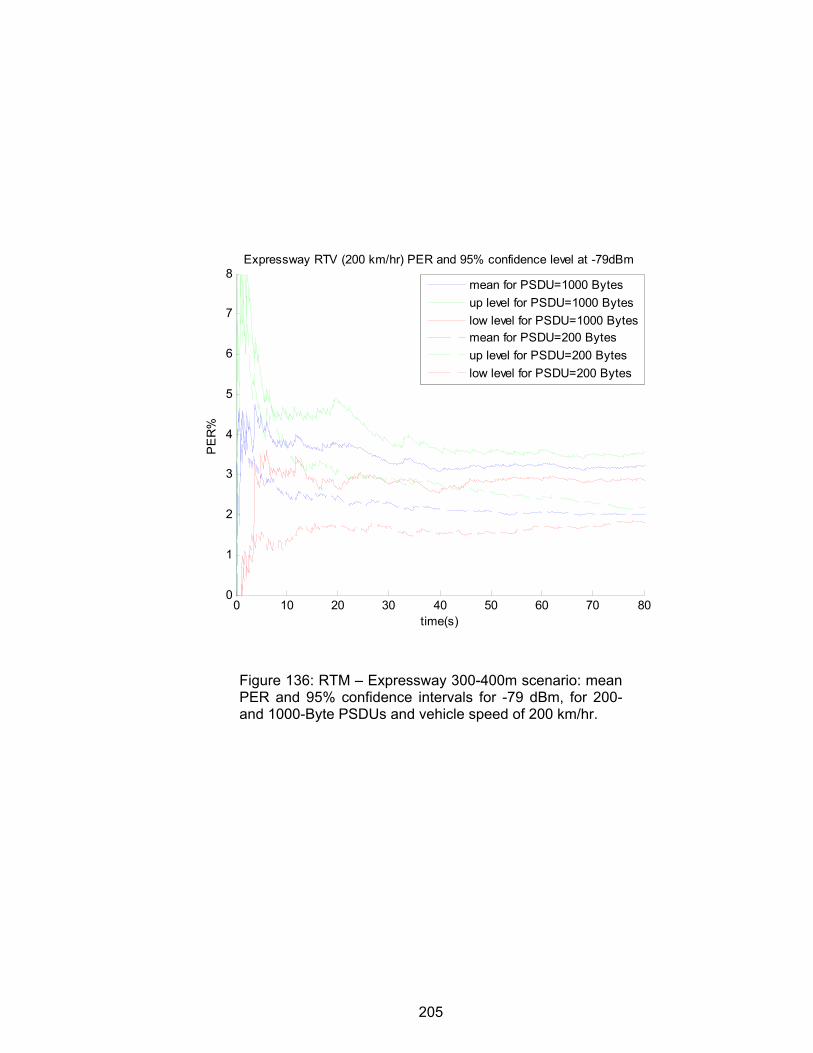
205

0 10 20 30 40 50 60 70 800

1

2

3

4

5

6

7

8

time(s)

PE

R%

Expressway RTV (200 km/hr) PER and 95% confidence level at -79dBm

mean for PSDU=1000 Bytesup level for PSDU=1000 Byteslow level for PSDU=1000 Bytesmean for PSDU=200 Bytesup level for PSDU=200 Byteslow level for PSDU=200 Bytes

Figure 136: RTM – Expressway 300-400m scenario: mean PER and 95% confidence intervals for -79 dBm, for 200- and 1000-Byte PSDUs and vehicle speed of 200 km/hr.

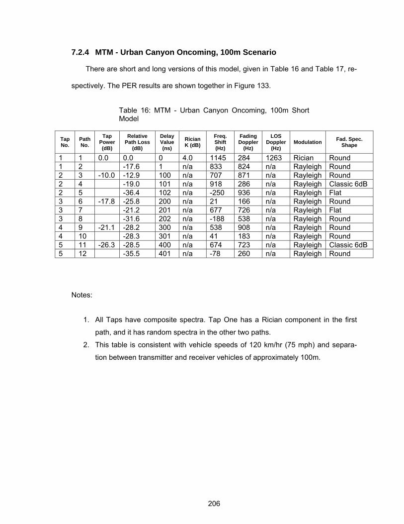
206

7.2.4 MTM - Urban Canyon Oncoming, 100m Scenario

There are short and long versions of this model, given in Table 16 and Table 17, re-

spectively. The PER results are shown together in Figure 133.

Table 16: MTM - Urban Canyon Oncoming, 100m Short Model

Tap No.

Path No.

Tap Power (dB)

Relative Path Loss

(dB)

Delay Value (ns)

Rician K (dB)

Freq. Shift (Hz)

Fading Doppler

(Hz)

LOS Doppler


Shape

1 1 0.0 0.0 0 4.0 1145 284 1263 Rician Round 1 2 -17.6 1 n/a 833 824 n/a Rayleigh Round 2 3 -10.0 -12.9 100 n/a 707 871 n/a Rayleigh Round 2 4 -19.0 101 n/a 918 286 n/a Rayleigh Classic 6dB 2 5 -36.4 102 n/a -250 936 n/a Rayleigh Flat 3 6 -17.8 -25.8 200 n/a 21 166 n/a Rayleigh Round 3 7 -21.2 201 n/a 677 726 n/a Rayleigh Flat 3 8 -31.6 202 n/a -188 538 n/a Rayleigh Round 4 9 -21.1 -28.2 300 n/a 538 908 n/a Rayleigh Round 4 10 -28.3 301 n/a 41 183 n/a Rayleigh Round 5 11 -26.3 -28.5 400 n/a 674 723 n/a Rayleigh Classic 6dB 5 12 -35.5 401 n/a -78 260 n/a Rayleigh Round

Notes:





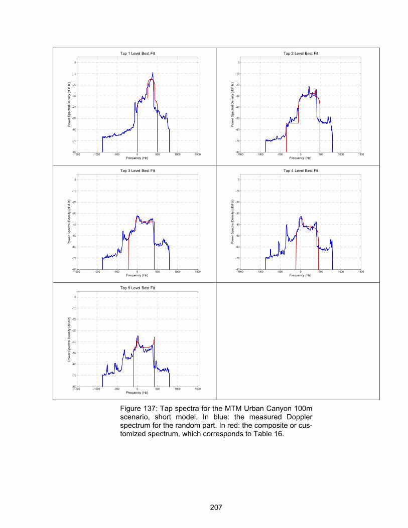
207

-1500 -1000 -500 0 500 1000 1500-80

-70

-60

-50

-40

-30

-20

-10

0


Pow

er S

pect

ral D

ensi

ty (d

B/H

z)

Frequency (Hz)-1500 -1000 -500 0 500 1000 1500

-80

-70

-60

-50

-40

-30

-20

-10

0


Pow

er S

pect

ral D

ensi

ty (d

B/H

z)

Frequency (Hz)

-1500 -1000 -500 0 500 1000 1500-80

-70

-60

-50

-40

-30

-20

-10

0


Pow

er S

pect

ral D

ensi

ty (d

B/H

z)

Frequency (Hz)-1500 -1000 -500 0 500 1000 1500

-80

-70

-60

-50

-40

-30

-20

-10

0


Pow

er S

pect

ral D

ensi

ty (d

B/H

z)

Frequency (Hz)

-1500 -1000 -500 0 500 1000 1500-80

-70

-60

-50

-40

-30

-20

-10

0


Pow

er S

pect

ral D

ensi

ty (d

B/H

z)

Frequency (Hz)

Figure 137: Tap spectra for the MTM Urban Canyon 100m scenario, short model. In blue: the measured Doppler spectrum for the random part. In red: the composite or cus-tomized spectrum, which corresponds to Table 16.

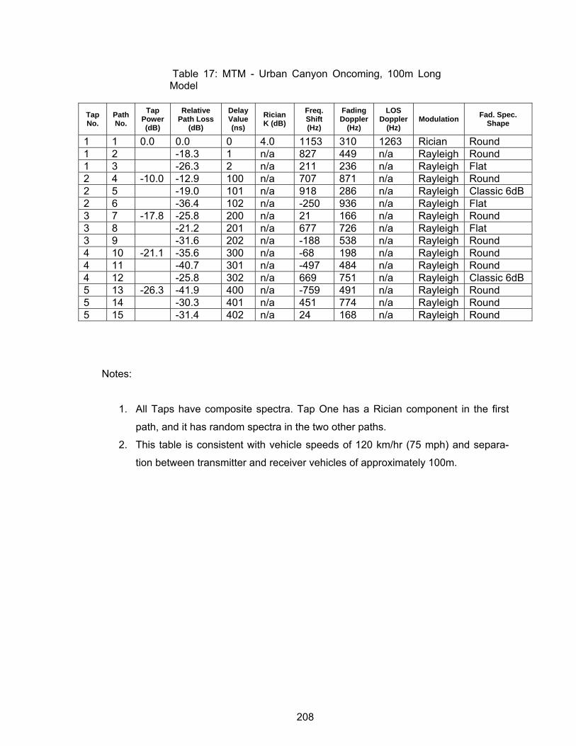
208

Table 17: MTM - Urban Canyon Oncoming, 100m Long Model

Tap No.

Path No.

Tap Power (dB)

Relative Path Loss

(dB)

Delay Value (ns)

Rician K (dB)

Freq. Shift (Hz)

Fading Doppler

(Hz)

LOS Doppler


Shape

1 1 0.0 0.0 0 4.0 1153 310 1263 Rician Round 1 2 -18.3 1 n/a 827 449 n/a Rayleigh Round 1 3 -26.3 2 n/a 211 236 n/a Rayleigh Flat 2 4 -10.0 -12.9 100 n/a 707 871 n/a Rayleigh Round 2 5 -19.0 101 n/a 918 286 n/a Rayleigh Classic 6dB 2 6 -36.4 102 n/a -250 936 n/a Rayleigh Flat 3 7 -17.8 -25.8 200 n/a 21 166 n/a Rayleigh Round 3 8 -21.2 201 n/a 677 726 n/a Rayleigh Flat 3 9 -31.6 202 n/a -188 538 n/a Rayleigh Round 4 10 -21.1 -35.6 300 n/a -68 198 n/a Rayleigh Round 4 11 -40.7 301 n/a -497 484 n/a Rayleigh Round 4 12 -25.8 302 n/a 669 751 n/a Rayleigh Classic 6dB 5 13 -26.3 -41.9 400 n/a -759 491 n/a Rayleigh Round 5 14 -30.3 401 n/a 451 774 n/a Rayleigh Round 5 15 -31.4 402 n/a 24 168 n/a Rayleigh Round

Notes:


path, and it has random spectra in the two other paths.



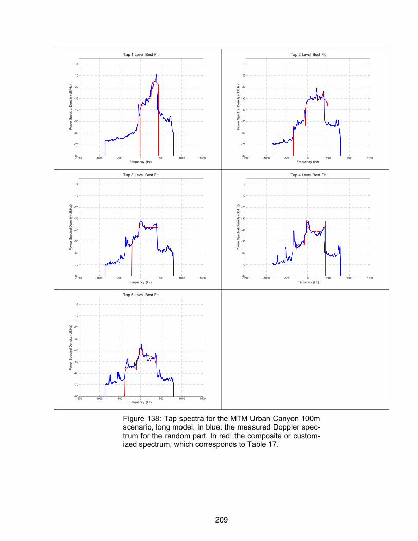
209

-1500 -1000 -500 0 500 1000 1500-80

-70

-60

-50

-40

-30

-20

-10

0


Pow

er S

pect

ral D

ensi

ty (d

B/H

z)

Frequency (Hz)-1500 -1000 -500 0 500 1000 1500

-80

-70

-60

-50

-40

-30

-20

-10

0


Pow

er S

pect

ral D

ensi

ty (d

B/H

z)

Frequency (Hz)

-1500 -1000 -500 0 500 1000 1500-80

-70

-60

-50

-40

-30

-20

-10

0


Pow

er S

pect

ral D

ensi

ty (d

B/H

z)

Frequency (Hz)-1500 -1000 -500 0 500 1000 1500

-80

-70

-60

-50

-40

-30

-20

-10

0


Pow

er S

pect

ral D

ensi

ty (d

B/H

z)

Frequency (Hz)

-1500 -1000 -500 0 500 1000 1500-80

-70

-60

-50

-40

-30

-20

-10

0


Pow

er S

pect

ral D

ensi

ty (d

B/H

z)

Frequency (Hz)

Figure 138: Tap spectra for the MTM Urban Canyon 100m scenario, long model. In blue: the measured Doppler spec-trum for the random part. In red: the composite or custom-ized spectrum, which corresponds to Table 17.

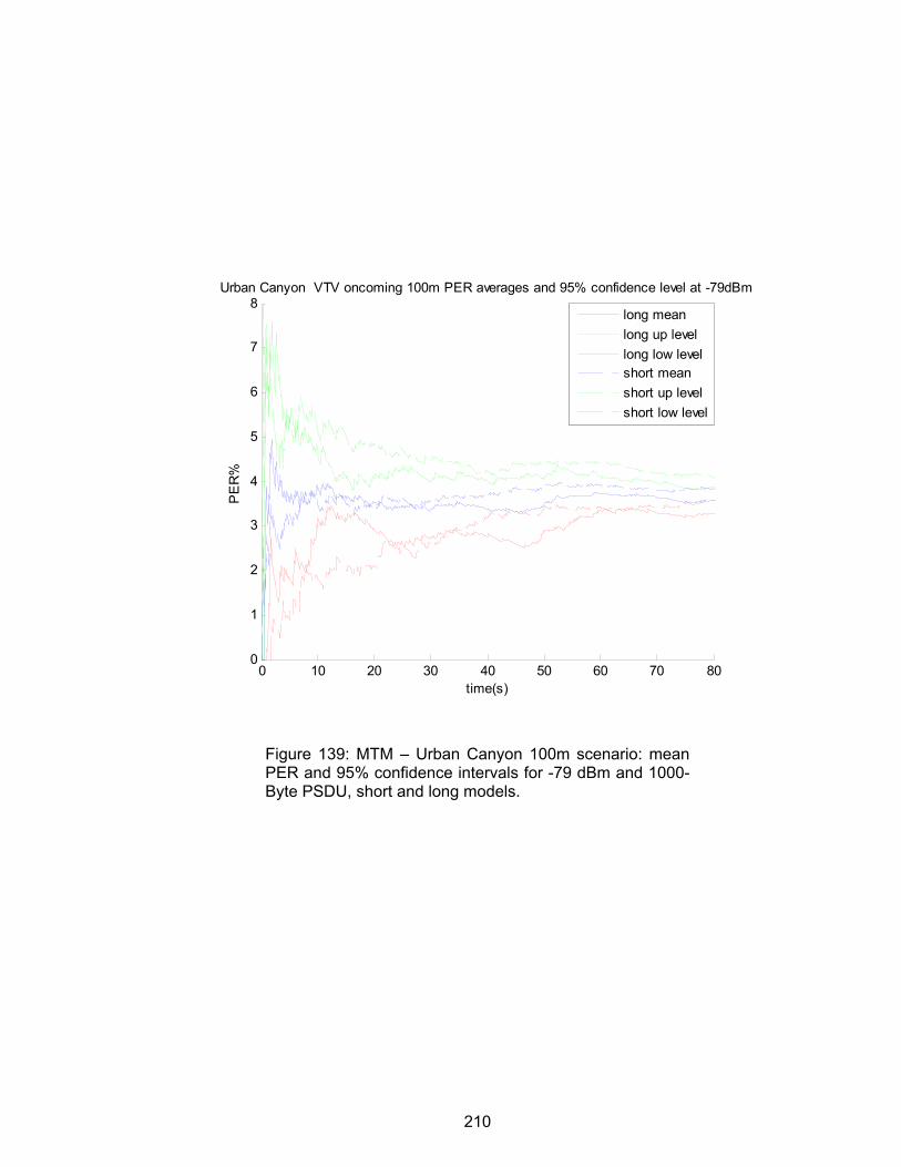
210

0 10 20 30 40 50 60 70 800

1

2

3

4

5

6

7

8

time(s)

PE

R%

Urban Canyon VTV oncoming 100m PER averages and 95% confidence level at -79dBm


Figure 139: MTM – Urban Canyon 100m scenario: mean PER and 95% confidence intervals for -79 dBm and 1000-Byte PSDU, short and long models.

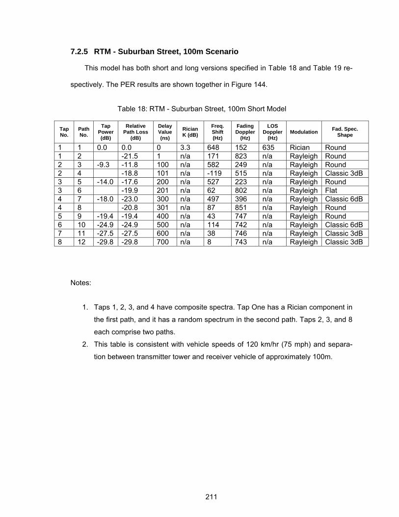
211

7.2.5 RTM - Suburban Street, 100m Scenario

This model has both short and long versions specified in Table 18 and Table 19 re-

spectively. The PER results are shown together in Figure 144.

Table 18: RTM - Suburban Street, 100m Short Model

Tap No.

Path No.

Tap Power (dB)

Relative Path Loss

(dB)

Delay Value (ns)

Rician K (dB)

Freq. Shift (Hz)

Fading Doppler

(Hz)

LOS Doppler


Shape

1 1 0.0 0.0 0 3.3 648 152 635 Rician Round 1 2 -21.5 1 n/a 171 823 n/a Rayleigh Round 2 3 -9.3 -11.8 100 n/a 582 249 n/a Rayleigh Round 2 4 -18.8 101 n/a -119 515 n/a Rayleigh Classic 3dB 3 5 -14.0 -17.6 200 n/a 527 223 n/a Rayleigh Round 3 6 -19.9 201 n/a 62 802 n/a Rayleigh Flat 4 7 -18.0 -23.0 300 n/a 497 396 n/a Rayleigh Classic 6dB 4 8 -20.8 301 n/a 87 851 n/a Rayleigh Round 5 9 -19.4 -19.4 400 n/a 43 747 n/a Rayleigh Round 6 10 -24.9 -24.9 500 n/a 114 742 n/a Rayleigh Classic 6dB 7 11 -27.5 -27.5 600 n/a 38 746 n/a Rayleigh Classic 3dB 8 12 -29.8 -29.8 700 n/a 8 743 n/a Rayleigh Classic 3dB

Notes:

1. Taps 1, 2, 3, and 4 have composite spectra. Tap One has a Rician component in

the first path, and it has a random spectrum in the second path. Taps 2, 3, and 8

each comprise two paths.



212

-1500 -1000 -500 0 500 1000 1500-80

-70

-60

-50

-40

-30

-20

-10

0


Pow

er S

pect

ral D

ensi

ty (d

B/H

z)

Frequency (Hz)-1500 -1000 -500 0 500 1000 1500

-80

-70

-60

-50

-40

-30

-20

-10

0


Pow

er S

pect

ral D

ensi

ty (d

B/H

z)Frequency (Hz)

-1500 -1000 -500 0 500 1000 1500-80

-70

-60

-50

-40

-30

-20

-10

0


Pow

er S

pect

ral D

ensi

ty (d

B/H

z)

Frequency (Hz)-1500 -1000 -500 0 500 1000 1500

-80

-70

-60

-50

-40

-30

-20

-10

0


Pow

er S

pect

ral D

ensi

ty (d

B/H

z)

Frequency (Hz)

Figure 140: First four tap spectra for the RTM Suburban Street 100m scenario, short model. In blue: the measured Doppler spectrum for the random part. In red: the compos-ite or customized spectrum, which corresponds to Table 18.

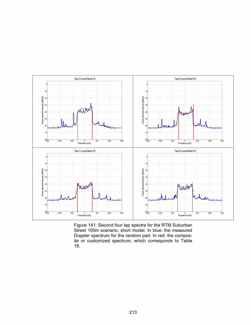
213

-1500 -1000 -500 0 500 1000 1500-80

-70

-60

-50

-40

-30

-20

-10

0


Pow

er S

pect

ral D

ensi

ty (d

B/H

z)

Frequency (Hz)-1500 -1000 -500 0 500 1000 1500

-80

-70

-60

-50

-40

-30

-20

-10

0


Pow

er S

pect

ral D

ensi

ty (d

B/H

z)Frequency (Hz)

-1500 -1000 -500 0 500 1000 1500-80

-70

-60

-50

-40

-30

-20

-10

0


Pow

er S

pect

ral D

ensi

ty (d

B/H

z)

Frequency (Hz)-1500 -1000 -500 0 500 1000 1500

-80

-70

-60

-50

-40

-30

-20

-10

0


Pow

er S

pect

ral D

ensi

ty (d

B/H

z)

Frequency (Hz)

Figure 141: Second four tap spectra for the RTM Suburban Street 100m scenario, short model. In blue: the measured Doppler spectrum for the random part. In red: the compos-ite or customized spectrum, which corresponds to Table 18.

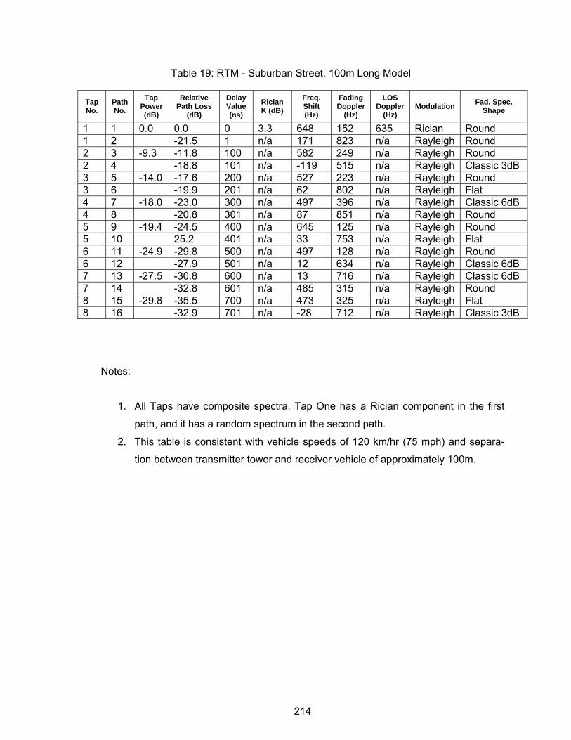
214

Table 19: RTM - Suburban Street, 100m Long Model

Tap No.

Path No.

Tap Power (dB)

Relative Path Loss

(dB)

Delay Value (ns)

Rician K (dB)

Freq. Shift (Hz)

Fading Doppler

(Hz)

LOS Doppler


Shape

1 1 0.0 0.0 0 3.3 648 152 635 Rician Round 1 2 -21.5 1 n/a 171 823 n/a Rayleigh Round 2 3 -9.3 -11.8 100 n/a 582 249 n/a Rayleigh Round 2 4 -18.8 101 n/a -119 515 n/a Rayleigh Classic 3dB 3 5 -14.0 -17.6 200 n/a 527 223 n/a Rayleigh Round 3 6 -19.9 201 n/a 62 802 n/a Rayleigh Flat 4 7 -18.0 -23.0 300 n/a 497 396 n/a Rayleigh Classic 6dB 4 8 -20.8 301 n/a 87 851 n/a Rayleigh Round 5 9 -19.4 -24.5 400 n/a 645 125 n/a Rayleigh Round 5 10 25.2 401 n/a 33 753 n/a Rayleigh Flat 6 11 -24.9 -29.8 500 n/a 497 128 n/a Rayleigh Round 6 12 -27.9 501 n/a 12 634 n/a Rayleigh Classic 6dB 7 13 -27.5 -30.8 600 n/a 13 716 n/a Rayleigh Classic 6dB 7 14 -32.8 601 n/a 485 315 n/a Rayleigh Round 8 15 -29.8 -35.5 700 n/a 473 325 n/a Rayleigh Flat 8 16 -32.9 701 n/a -28 712 n/a Rayleigh Classic 3dB

Notes:


path, and it has a random spectrum in the second path.



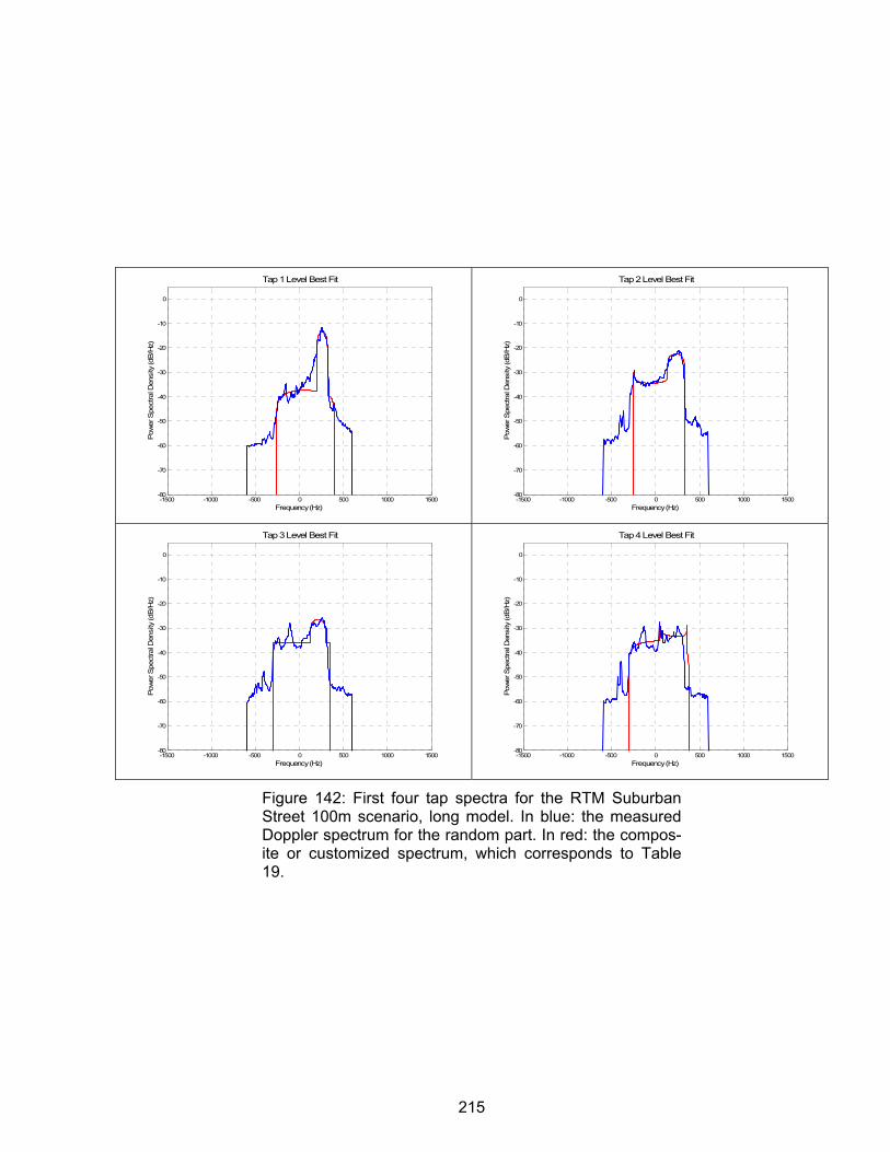
215

-1500 -1000 -500 0 500 1000 1500-80

-70

-60

-50

-40

-30

-20

-10

0


Pow

er S

pect

ral D

ensi

ty (d

B/H

z)

Frequency (Hz)-1500 -1000 -500 0 500 1000 1500

-80

-70

-60

-50

-40

-30

-20

-10

0


Pow

er S

pect

ral D

ensi

ty (d

B/H

z)Frequency (Hz)

-1500 -1000 -500 0 500 1000 1500-80

-70

-60

-50

-40

-30

-20

-10

0


Pow

er S

pect

ral D

ensi

ty (d

B/H

z)

Frequency (Hz)-1500 -1000 -500 0 500 1000 1500

-80

-70

-60

-50

-40

-30

-20

-10

0


Pow

er S

pect

ral D

ensi

ty (d

B/H

z)

Frequency (Hz)

Figure 142: First four tap spectra for the RTM Suburban Street 100m scenario, long model. In blue: the measured Doppler spectrum for the random part. In red: the compos-ite or customized spectrum, which corresponds to Table 19.

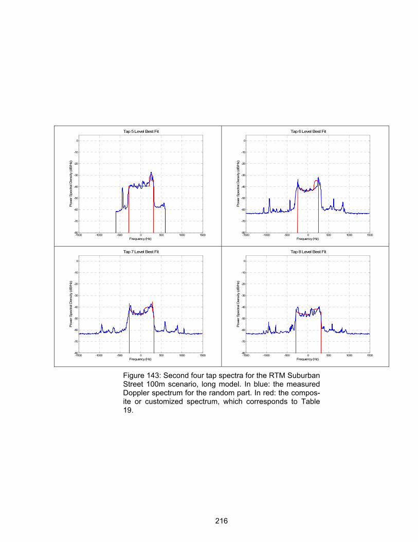
216

-1500 -1000 -500 0 500 1000 1500-80

-70

-60

-50

-40

-30

-20

-10

0


Pow

er S

pect

ral D

ensi

ty (d

B/H

z)

Frequency (Hz)-1500 -1000 -500 0 500 1000 1500

-80

-70

-60

-50

-40

-30

-20

-10

0


Pow

er S

pect

ral D

ensi

ty (d

B/H

z)Frequency (Hz)

-1500 -1000 -500 0 500 1000 1500-80

-70

-60

-50

-40

-30

-20

-10

0


Pow

er S

pect

ral D

ensi

ty (d

B/H

z)

Frequency (Hz)-1500 -1000 -500 0 500 1000 1500

-80

-70

-60

-50

-40

-30

-20

-10

0


Pow

er S

pect

ral D

ensi

ty (d

B/H

z)

Frequency (Hz)

Figure 143: Second four tap spectra for the RTM Suburban Street 100m scenario, long model. In blue: the measured Doppler spectrum for the random part. In red: the compos-ite or customized spectrum, which corresponds to Table 19.

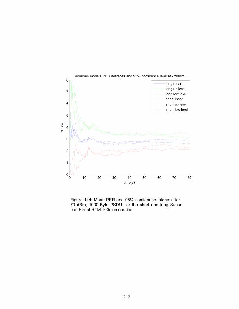
217

0 10 20 30 40 50 60 70 800

1

2

3

4

5

6

7

8

time(s)

PE

R%

Suburban models PER averages and 95% confidence level at -79dBm


Figure 144: Mean PER and 95% confidence intervals for -79 dBm, 1000-Byte PSDU, for the short and long Subur-ban Street RTM 100m scenarios.

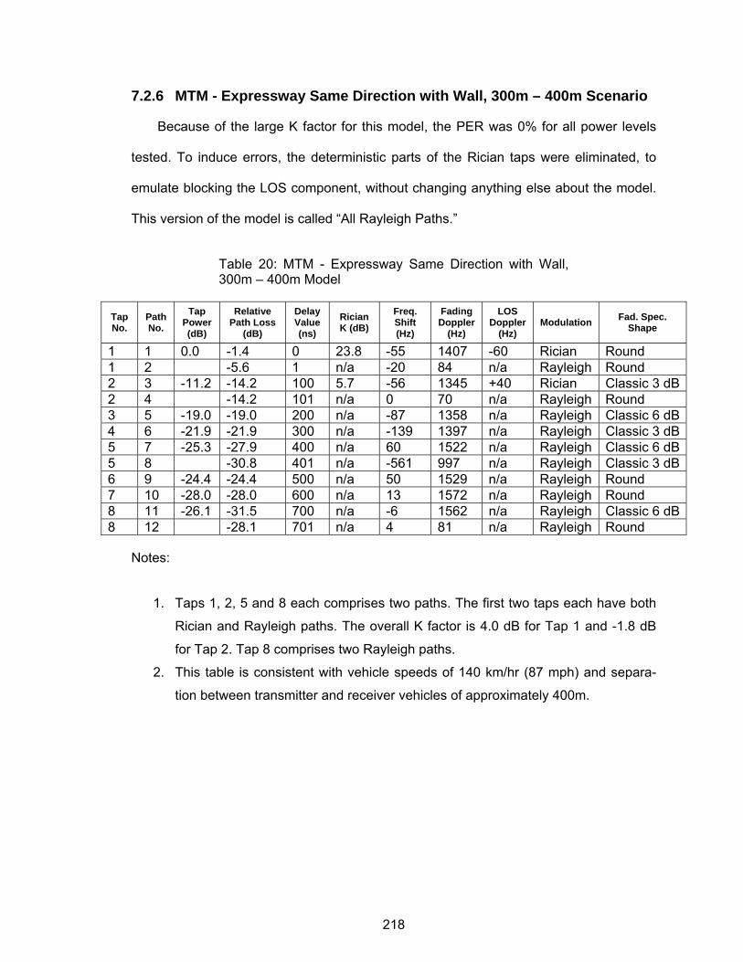
218

7.2.6 MTM - Expressway Same Direction with Wall, 300m – 400m Scenario

Because of the large K factor for this model, the PER was 0% for all power levels

tested. To induce errors, the deterministic parts of the Rician taps were eliminated, to

emulate blocking the LOS component, without changing anything else about the model.

This version of the model is called “All Rayleigh Paths.”

Table 20: MTM - Expressway Same Direction with Wall, 300m – 400m Model

Tap No.

Path No.

Tap Power (dB)

Relative Path Loss

(dB)

Delay Value (ns)

Rician K (dB)

Freq. Shift (Hz)

Fading Doppler

(Hz)

LOS Doppler


Shape

1 1 0.0 -1.4 0 23.8 -55 1407 -60 Rician Round 1 2 -5.6 1 n/a -20 84 n/a Rayleigh Round 2 3 -11.2 -14.2 100 5.7 -56 1345 +40 Rician Classic 3 dB2 4 -14.2 101 n/a 0 70 n/a Rayleigh Round 3 5 -19.0 -19.0 200 n/a -87 1358 n/a Rayleigh Classic 6 dB4 6 -21.9 -21.9 300 n/a -139 1397 n/a Rayleigh Classic 3 dB5 7 -25.3 -27.9 400 n/a 60 1522 n/a Rayleigh Classic 6 dB5 8 -30.8 401 n/a -561 997 n/a Rayleigh Classic 3 dB6 9 -24.4 -24.4 500 n/a 50 1529 n/a Rayleigh Round 7 10 -28.0 -28.0 600 n/a 13 1572 n/a Rayleigh Round 8 11 -26.1 -31.5 700 n/a -6 1562 n/a Rayleigh Classic 6 dB8 12 -28.1 701 n/a 4 81 n/a Rayleigh Round

Notes:

1. Taps 1, 2, 5 and 8 each comprises two paths. The first two taps each have both

Rician and Rayleigh paths. The overall K factor is 4.0 dB for Tap 1 and -1.8 dB

for Tap 2. Tap 8 comprises two Rayleigh paths.



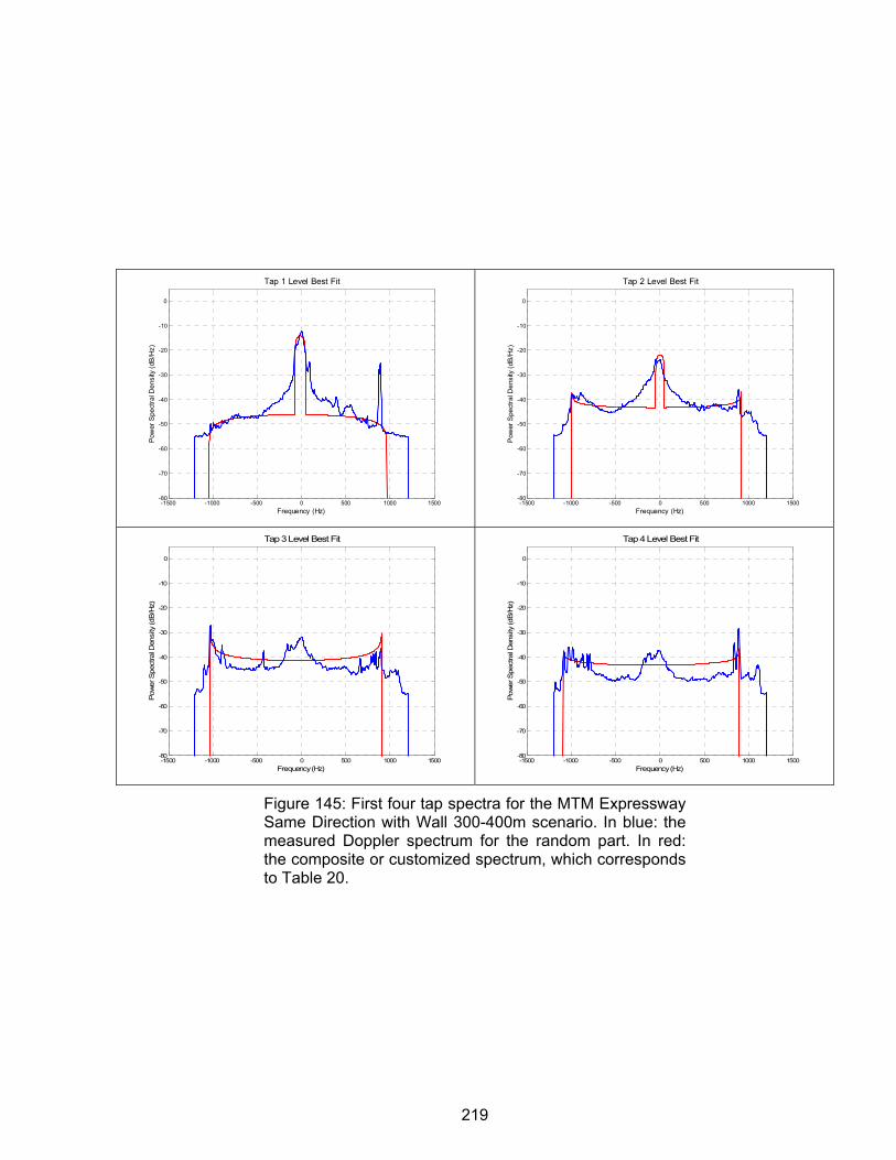
219

-1500 -1000 -500 0 500 1000 1500-80

-70

-60

-50

-40

-30

-20

-10

0


Pow

er S

pect

ral D

ensi

ty (d

B/H

z)

Frequency (Hz)-1500 -1000 -500 0 500 1000 1500

-80

-70

-60

-50

-40

-30

-20

-10

0


Pow

er S

pect

ral D

ensi

ty (d

B/H

z)Frequency (Hz)

-1500 -1000 -500 0 500 1000 1500-80

-70

-60

-50

-40

-30

-20

-10

0


Pow

er S

pect

ral D

ensi

ty (d

B/H

z)

Frequency (Hz)-1500 -1000 -500 0 500 1000 1500

-80

-70

-60

-50

-40

-30

-20

-10

0


Pow

er S

pect

ral D

ensi

ty (d

B/H

z)

Frequency (Hz)

Figure 145: First four tap spectra for the MTM Expressway Same Direction with Wall 300-400m scenario. In blue: the measured Doppler spectrum for the random part. In red: the composite or customized spectrum, which corresponds to Table 20.

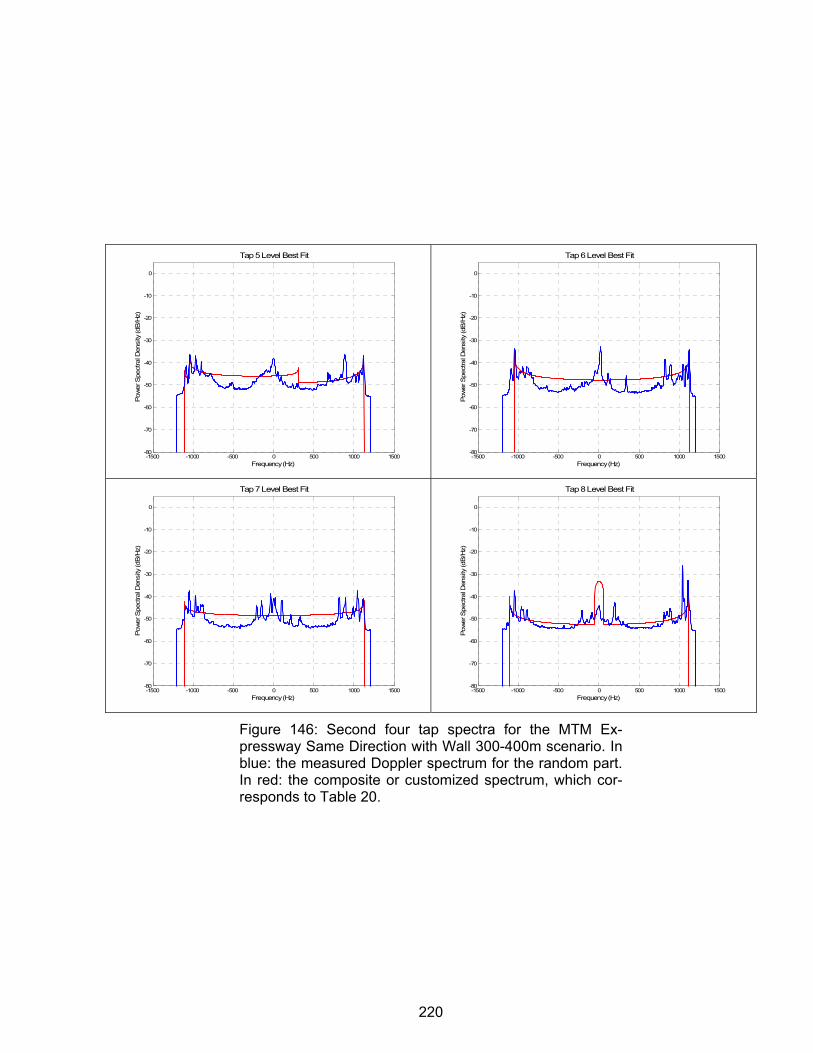
220

-1500 -1000 -500 0 500 1000 1500-80

-70

-60

-50

-40

-30

-20

-10

0


Pow

er S

pect

ral D

ensi

ty (d

B/H

z)

Frequency (Hz)-1500 -1000 -500 0 500 1000 1500

-80

-70

-60

-50

-40

-30

-20

-10

0


Pow

er S

pect

ral D

ensi

ty (d

B/H

z)Frequency (Hz)

-1500 -1000 -500 0 500 1000 1500-80

-70

-60

-50

-40

-30

-20

-10

0


Pow

er S

pect

ral D

ensi

ty (d

B/H

z)

Frequency (Hz)-1500 -1000 -500 0 500 1000 1500

-80

-70

-60

-50

-40

-30

-20

-10

0


Pow

er S

pect

ral D

ensi

ty (d

B/H

z)

Frequency (Hz)

Figure 146: Second four tap spectra for the MTM Ex-pressway Same Direction with Wall 300-400m scenario. In blue: the measured Doppler spectrum for the random part. In red: the composite or customized spectrum, which cor-responds to Table 20.

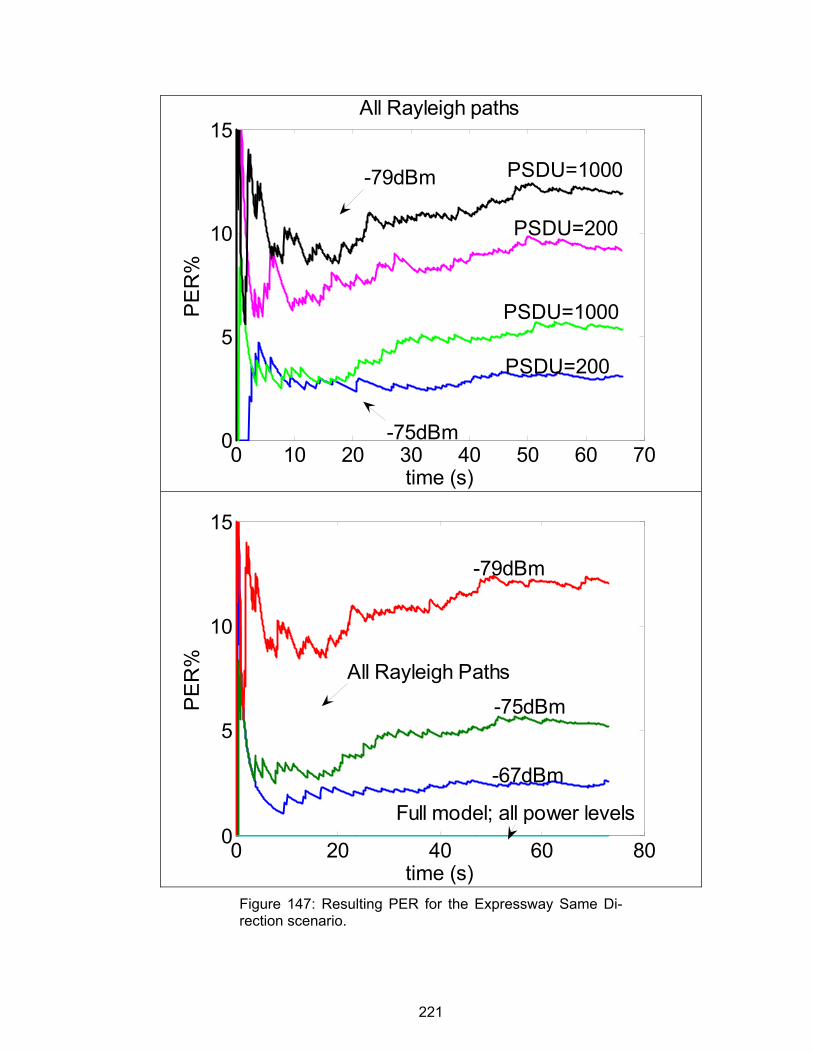
221

Figure 147: Resulting PER for the Expressway Same Di-rection scenario.

0 20 40 60 800

5

10

15

time (s)

PE

R% All Rayleigh Paths

-79dBm

-75dBm

-67dBm

Full model; all power levels

0 10 20 30 40 50 60 700

5

10

15

time (s)

PE

R%

All Rayleigh paths

-75dBm

-79dBm PSDU=1000

PSDU=200

PSDU=200

PSDU=1000

222

CHAPTER 8

CONCLUSIONS

In this final chapter, we summarize the contributions of this dissertation. We also

present the future work that can result from the extension of the ideas and results pre-

sented.

8.1 Contributions • Combined sounding waveform: We were able to combine two pulse compres-

sion techniques in our channel sounding waveform. This way, we were able to

obtain the maximum dynamic range from our system with the MLS section, and

to use the full RF bandwidth available with the OFDM section.

• OFDM synchronization for design stage: We have presented an algorithm that

allows the identification and compensation of all the static OFDM synchronization

offsets. This algorithm is intended for systems where the timing clock is not ac-

cessible such as the software radio system that we could develop with the

Pentek™ modular system used in this project.

• Recorded channel in simulation: We developed a reliable simulated receiver

system to compare the behavior of a real recorded channel to the behavior of

any proposed synthesized channel. We included all the specifications indicated

by the WAVE/DSRC standard and most of the processing required in a similar

system.

223

• Model methodology: We have showed the necessity of more comprehensive

channel model methodology for the high mobility channels under study. We

started with the popular techniques found in the literature, and we grew from

them to propose extended methodologies that capture more of the dynamics

present in these types of channels. In particular, we were able to show the corre-

lation between the K-factor and the BER using our also developed system to in-

tegrate the recorded channel in simulations.

• Finished Models: We have presented six models, suitable for simulation on

standard RF channel emulators, representing three MTM and three RTM envi-

ronments measured in the Atlanta, Georgia metropolitan area. The models were

ranked in terms of PER measured at -79 dBm with 1000-byte PSDUs, and the

MTM Expressway without Wall channel had the highest measured PER. There-

fore, this is the model we recommend for the WAVE/DSRC certification test, be-

cause if equipment passes the certification test with this channel it is likely that it

will pass the other channels as well. Three of the models, RTM Urban Canyon,

MTM Urban Canyon, and RTM Suburban Street, had both long and short ver-

sions (greater than 12 paths and less than or equal to 12 paths, respectively). Of

these, the only long-short pair that produced statistically different mean PERs

was the first, and for that one, the mean PERs differed by less than 0.5%. There-

fore, the long-short distinction is not very important from a link performance point

of view.

8.2 Suggested Future Work • Include MTM channel in the combined effects of OFDM synchronization

offsets: In (3.25) and (3.29), we presented the degradation produced by just

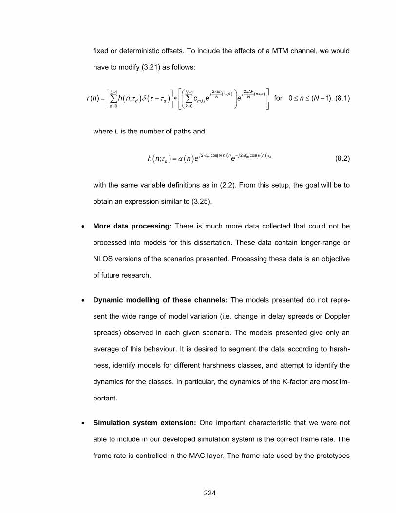
224

fixed or deterministic offsets. To include the effects of a MTM channel, we would

have to modify (3.21) as follows:

( ) ( ) ( ) ( )2 21 1 1

, ,0 0

( ) ; for 0 ( 1).kn FL N j j n

N Nd d m l i

d kr n h n c e e n N

π πβ ατ δ τ τ

Δ− − + +

= =

⎡ ⎤⎛ ⎞⎡ ⎤= − ∗ ≤ ≤ −⎢ ⎥⎜ ⎟⎢ ⎥⎣ ⎦ ⎢ ⎥⎝ ⎠⎣ ⎦∑ ∑ (8.1)

where L is the number of paths and

( ) ( ) ( )( ) ( )( )2 cos 2 cos; m m dj f n n j f ndh n n e eπ θ π θ ττ α −= (8.2)

with the same variable definitions as in (2.2). From this setup, the goal will be to

obtain an expression similar to (3.25).

• More data processing: There is much more data collected that could not be

processed into models for this dissertation. These data contain longer-range or

NLOS versions of the scenarios presented. Processing these data is an objective

of future research.

• Dynamic modelling of these channels: The models presented do not repre-

sent the wide range of model variation (i.e. change in delay spreads or Doppler

spreads) observed in each given scenario. The models presented give only an

average of this behaviour. It is desired to segment the data according to harsh-

ness, identify models for different harshness classes, and attempt to identify the

dynamics for the classes. In particular, the dynamics of the K-factor are most im-

portant.

• Simulation system extension: One important characteristic that we were not

able to include in our developed simulation system is the correct frame rate. The

frame rate is controlled in the MAC layer. The frame rate used by the prototypes

225

is much lower than the one we used in our simulations. All of our results in com-

paring real to synthesized or simulated channels assume a continuous frame

rate, i.e., one frame after another without spaces, and we compare transmitted

vs. received data to obtain the BER. We have a significant period between

frames in the prototypes, and there is no transmitted vs. received data compari-

son; therefore, any further comparison between real or recorded channel vs. a

proposed model should have a matched frame rate and the same type of error

metric.

• MIMO extension: The GTRI recording and transmission system used in the

measurement campaign has the possibility to grow into a MIMO system. In par-

ticular, the system used for Phase Two is ready for a 2x2 MIMO up to 3 GHz.

The combined sounding waveform can also be modified for MIMO. We can sub-

situte the MLS section with a Gold sequence, and we can use an odd/even sub-

carrier separation in the OFDM section.

226

REFERENCES

[1] A. Abdi, C. Tepedelenlioglu, M. Kaveh, and G. Giannakis, “On the estimation of the K pa-rameter for the Rice fading distribution,” in IEEE Communications Letters, vol. 5, No. 3, pp. 92-94, March 2001.

[2] G. Acosta, K. Tokuda, and M. A. Ingram, “Measured joint Doppler-delay power profiles for vehicle-to-vehicle communications at 2.4 GHz,” in Proc. of IEEE Global Telecom. Conf., vol. 6, pp. 3813-3817, 2004.

[3] Guillermo Acosta and Mary Ann Ingram, “Model development for the wideband vehicle-to-vehicle 2.4 GHz channel,” Proc. IEEE Wireless Communications & Networking Conference (WCNC 2006), Las Vegas, NV, 3-6 April 2006.

[4] G. Acosta-Marum and M.A. Ingram, “A BER-Based Partitioned Model for a 2.4 GHz Vehicle-to-Vehicle Expressway Channel,” in International Journal on Wireless Personal Communica-tion, July 2006.

[5] J. B. Andersen, “Radio channel characterization,” in COST 231 Final Report.

[6] ASTM E 2213-03, “Standard Specification for Telecommunications and Information Ex-change between Roadside and Vehicle Systems— 5.9 GHz Band Dedicated Short Range Communications (DSRC) Medium Access Control (MAC) and Physical Layer (PHY) Specifi-cations,” ASTM International, www.astm.org.

[7] A. S. Akki and F. Haber, “A statistical model of mobile-to-mobile land communication chan-nel,” in IEEE Transactions on Vehicular Technology, pp. 2–7, February 1986.

[8] A. S. Akki, “Statistical properties of mobile-to-mobile land communication channels,” in IEEE Transactions on Vehicular Technology, vol. 43, No. 4, November 1994.

[9] H. Bantli, E. Ring, and E. Goff, “Requirements for direct short range, vehicle to roadside communications,” in Proceedings of the IEEE Aerospace Conference, pp. 46-61, Feb. 1997.

[10] J. J. van de Beek, M. Sandell, and P. O. Borjesson, “ML estimation of time and frequency offset in OFDM systems,” in IEEE Transactions on Signal Processing, vol. 45, pp. 1800-1805, July 1997

[11] P. A. Bello, “Characterization of randomly time-variant linear channels,” in IEEE Transactions on Communication Systems, vol. 11, pp. 360-393, December 1963.

[12] J. Bingham, “Method and apparatus for correcting for clock and carrier frequency offset, and phase jitter in multicarrier modems.” U.S. Patent No. 5206886, April 27, 1993.

[13] W. R. Braun and U. Dersch, “A physical mobile radio channel model,” in IEEE Transactions on Vehicular Technology, vol. 40, No. 2, pp. 472-482, May 1991.

[14] X. Cai and G.B. Giannakis, “Bounding performance and suppressing intercarrier interference in wireless mobile OFDM,” IEEE Trans. Comm. Vol. 51, No. 12, December 2003.

227

[15] http://www.channelsounder.de (May, 2005).

[16] C-C. Chong, C-M. Tan, D. I. Laurenson, S. McLaughlin, M. A. Beach, and A. R. Nix, “A novel wideband dynamic directional indoor channel model based on a Markov process,” in IEEE Transactions on Wireless Communications, vol. 4, No. 4, pp. 1539-1552, July 2005.

[17] F. Classen and H. Meyr, “Frequency synchronization algorithms for OFDM systems suitable for communication over frequency selective fading channels,” in Proceedings of IEEE the Global Telecommunications Conference, vol.3, pp. 1655-1659, 1994.

[18] T. de Couasnon, R. Monnier, and J. Rault, “OFDM for digital TV broadcasting,” Signal Proc-essing, vol. 39, pp. 1-32, 1994.

[19] A. J. Coulson, “Maximum likelihood synchronization for OFDM using a pilot symbol: Algo-rithms,” in the IEEE Journal on Selected Areas in Communications, vol. 19, pp. 2486–2494, December 2001.

[20] A.J. Coulson, “Maximum likelihood synchronization for OFDM using a pilot symbol: Analysis,” in the IEEE Journal on Selected Areas in Communications, vol. 19, pp. 2495–2502, Decem-ber 2001.

[21] D. C. Cox, “Delay Doppler characteristics of multipath propagation at 910 MHz in a suburban mobile radio environment,” in IEEE Transactions on Antennas and Propagation, vol. 20, No. 5, pp. 625-635, September 1972.

[22] A. V. B. Da Silva and M. Nakagawa, “Radio wave propagation measurements in tunnel en-trance environment for intelligent transportation systems applications,” in Proceedings of the IEEE Intelligent Transportation Systems Conference, pp. 883-888, August 2001.

[23] F. Daffara and O. Adami, “A new frequency detector for orthogonal multicarrier transmission techniques,” in Proceedings of the IEEE Vehicular Technology Conference, vol.2, pp. 804-809, 1995.

[24] F. Daffara and A. Chouly, “Maximum likelihood frequency detectors for orthogonal multicar-rier systems,” in Proceedings of the 1993 IEEE International Conference in Communications, pp. 766-771.

[25] J. S. Davis II and J. P. Linnartz, “Vehicle to vehicle RF propagation measurements,” in Pro-ceedings of the Twenty-Eighth Asilomar Conference on Signals, Systems and Computers, pp. 470–474, October 1994.

[26] C.R. Dow, P. J. Lin, S. C. Chen, J. H. Lin, and S. F. Hwang, “A study of recent research trends and experimental guidelines in mobile ad-hoc network,” in Proc. of Advanced Informa-tion Networking and Applications 19th International Conference, vol.1, pp. 72-77, March 2005.

[27] P. G. Flikkema and S. G. Johnson, “A comparison of time- and frequency-domain wireless channel sounding techniques,” in Proceedings of the IEEE Southeastcon ’96. ‘Bringing To-gether Education, Science and Technology,’ Tampa, FL USA, pp. 488-491, 11-14 April 1996.

[28] H. Gharavi and K. Ban, “Multihop sensor network design for wide-band communications,” IEEE Proceedings, Vol. 91, No. 8, pp. 1221–1234, August 2003.

228

[29] L. J. Greenstein, D. G. Michelson, and V. Erceg, “Moment-method estimation of the Ricean K-factor,” in IEEE Communications Letters, vol. 3, No. 6, pp. 175-176, June 1999.

[30] L. Hanzo, W. Webb, and T. Keller, Single- and Multi-carrier Quadrature Amplitude Modulation Principles and Applications for Personal Communications, WLANs and Broadcasting, Chich-ester, West Sussex, UK: John Wiley & Sons, Ltd, 2000.

[31] T. J. Harrold, A.R. Nix, and M.A. Beach, “Propagation studies for mobile-to-mobile communi-cations,” in Proc. of IEEE Vehicular Technology Conf., vol. 3, pp. 1251-1255, October 2001.

[32] Y. Higa and H. Furukawa, “One-way relay for wireless multihop networks associated with the intermittent periodic transmit and the spiral mesh routing,” in Proc. of IEEE Vehicular Tech-nology Conf., vol. 5, pp. 3202-3206, May 2005.

[33] M. H. Hsieh and C. H. Wei, “Channel estimation for OFDM systems based on comb-type pilot arrangement in frequency selective channels,” in IEEE Transactions on Consumer Electron-ics, vol. 44, No. 1, pp. 217-225, February 1998.

[34] http://ideas.repec.org/c/cod/matlab/ga.html (February, 2007).

[35] IEEE Std 502.11a-1999. Part 11: Wireless LAN Medium Access Control (MAC) and Physical Layer (PHY) Specifications: High-speed Physical Layer in the 5 GHz Band.

[36] W. C. Jakes, Microwave Mobile Communications, IEEE Press, New York, 1993.

[37] M. C. Jeruchim, P. Balaban, and K. S. Shanmugan, Simulation of Communication Systems: Modeling, Methodology, and Techniques, Second Edition, Kluwer Academic Press, Boston 2000.

[38] J-S. Jiang and M.A. Ingram, "Enhancing measured MIMO capacity by adapting the locations of the antenna elements," in Proceedings of the IEEE International Symposium on Per-sonal, Indoor, and Mobile Radio Communications, vol.3, pp. 1027-1031, 2002.

[39] Zhu Jing and S. Roy, “MAC for dedicated short range communications in intelligent transport system,” in IEEE Communications Magazine, Vol. 41, No. 12, pp. 60-67, December 2003.

[40] G. Kadel, “Propagation measurements and their analysis,” in COST 231 Final Report.

[41] G. Karam, F. Daffara, and H. Sari, “Simplified versions of the maximum-likelihood frequency detector,” in Proceedings of the. 1992 IEEE Global Telecommunications Conference, vol. 1, pp. 345-349.

[42] S. Kato, S. Tsugawa, K. Tokuda, T. Matsui, and H. Fujii, “Vehicle control algorithms for coop-erative driving with automated vehicles and intervehicle communications,” in IEEE Transac-tions on Intelligent Transportation Systems, pp. 155-161, September 2002

[43] J. Kivinen, X. Zhao, and P. Vainikainen, “Empirical characterization of wideband indoor radio channel at 5.3 GHz,” in IEEE Transactions on Antennas and Propagation, vol. 49, No. 8, Au-gust 2001.

[44] T. Kobayashi, H. Masui, S. Takahashi, K. Takahashi, and K. Kage, “Delay profile measure-ment system for microwave mobile communications and delay characteristics in an urban en-

http://users.ece.gatech.edu/~jsjiang�

http://users.ece.gatech.edu/~mai�

http://users.ece.gatech.edu/~mai/publication/jsjiang/PIMRC2002_Jiang_Web.pdf�

http://users.ece.gatech.edu/~mai/publication/jsjiang/PIMRC2002_Jiang_Web.pdf�

229

vironment,” in Proceedings of the IEEE Radio and Wireless Conference (RAWCON), pp. 163–166, August 1999.

[45] W. C. Y. Lee, “Estimate of local average power of mobile radio signal,” in IEEE Transactions on Vehicular Technology, vol. 34, No. 1, pp. 22-27, February 1985.

[46] Y. Li, L. J. Cimini, Jr., and N. R. Sollenberger, “Robust channel estimation for OFDM systems with rapid dispersive fading channels,” in IEEE Transactions on Communications, vol. 46, no. 7, pp. 902-915, July 1998.

[47] U. Martin, “Echo estimation-deriving simulation models for the mobile radio channel,” in Pro-ceedings of the Vehicular Technology Conference, vol. 1, pp. 231-235, July 1995.

[48] J. Maurer, T. Fügen, and W. Wiesbeck, “Narrow-band measurement and analysis of the inter-vehicle transmission channel at 5.2 GHz,” in Proceedings of the Vehicular Technology Con-ference, pp. 1274–1278, May 2002.

[49] H. Meyr, M. Moeneclaey, and S. A. Fechtel, Digital Communication Receivers: Synchroniza-tion, Channel Estimation, and Signal Processing, John Wiley & Sons, New York, 1998.

[50] A. N. Mody, “Signal Acquisition and Tracking for Fixed Wireless Access Multiple Input Multi-ple Output Orthogonal Frequency Division Multiplexing,” Ph.D. Thesis, Georgia Institute of Technology, Atlanta, Georgia 2004.

[51] W. Mohr, “Modeling of wideband mobile radio channels based on propagation measure-ments,” in Proc. 16th International Symposium of Personal, Indoor, Mobile Radio Communica-tions, vol. 2, pp. 397-401, 1995.

[52] M. Morelli, A. N. D’Andrea, and U. Mengali, “Feedback frequency synchronization for OFDM applications,” in Proceedings of the IEEE Global Telecommunications Conference, vol.5, pp. 2504-2507, 1999.

[53] Y. Morioka, T. Sota, T, and M. Nakagawa, “An anti-car collision system using GPS and 5.8 GHz inter-vehicle communication at an off-sight intersection,” in Proceedings of the IEEE Ve-hicular Technology Conference, pp. 2019-2024, September 2000.

[54] P. H. Moose, “A technique for orthogonal frequency division multiplexing frequency offset correction,” in IEEE Transactions on Communications, vol. 42, no. 10, pp. 2908-2914, Octo-ber 1994.

[55] K. H. Mueller, and M. S. Muller, "Timing recovery in digital synchronous data receivers," in IEEE Transactions on Communications, vol. COM-24, pp. 516-531, May 1976.

[56] R. V. Nee and R. Prasad, OFDM Wireless Multimedia Communications, Norwood, MA: Artech House, 2000.

[57] M. Newton, D. Kitchener, and M. S. Smith, “Wideband channel dynamics (measurement and simulation),” in Proc. of 11th International Antennas and Propagation Conf., pp. 428-431, April 2001.

[58] J. O. Nielsen, V. Afanassiev, and J. B. Andersen, “A dynamic model for the indoor channel,” in KAP Journal of Wireless Personal Communications, vol. 19, pp. 91-120, 2001.

230

[59] H. Nogami and T. Nagashima, “A frequency and timing period acquisition technique for OFDM systems,” in Proceedings of IEEE Personal, Indoor, and Mobile Radio Communica-tion, pp. 1010-1015, September 1995.

[60] Heo Nojeong and P. K. Varshney, “Energy-efficient deployment of intelligent mobile sensor networks,” IEEE Transactions on Systems, Man and Cybernetics, Vol. 35, No. 1, pp. 78–92, January 2005.

[61] K. K. Onodera and P. R. Gray, “A 75-mW 128-MHz DS-CDMA baseband demodulator for high-speed wireless applications,” in IEEE Journal of Solid-State Circuits, vol. 33, No. 5, pp. 753-760, May 1998.

[62] A. Papoulis, Probability, Random Variables, and Stochastic Processes, McGraw-Hill, New York, 1991.

[63] C. S. Patel, G. L. Stüber, and T. G. Pratt, “Simulation of Rayleigh faded mobile-to-mobile communication channels,” in Proceedings of the IEEE Vehicular Technology Conference, vol.1, pp. 163-167, October 2003.

[64] J. D. Parsons, D.A. Demery and A.M.D. Turkmani, “Sounding techniques for wideband mo-bile radio channels: a review,” in IEE Proceedings, pp. 437-446, Feb. 1991.

[65] T. Pollet, M. van Bladel, and M. Moeneclaey, “BER sensitivity of OFDM systems to carrier frequency offset and Wiener phase noise,” in IEEE Transactions on Communications, vol. 43, No. 2/3/4, pp. 191-193, February/March/April 1995.

[66] J. G. Proakis, Digital Communications, McGraw-Hill, New York, 1995.

[67] T. S. Rappaport, Wireless Communications: Principles and Practice, Prentice Hall PTR, Up-per Saddle River, NJ, 1995.

[68] J. S. Sadowsky and V. Kafedziski, “On the correlation and scattering functions of the WSSUS channel for mobile communications,” in IEEE Transactions on Vehicular Technology, vol. 1, No. 1, pp. 270-282, February 1998.

[69] S. Salous, P. Pantzaris, and P. Green, “FMCW waveforms for UHF/SHF wideband channel sounders,” in Proceedings of the IEE Colloquium on High Bit Rate UHF/SHF Channel Sounder Technology and Measurement, digest No. 1993/233, pp. 2/1-2/5.

[70] M. Sandell, J.-J. van de Beek, and P. O. Börjesson, “Timing and frequency synchronization in OFDM systems using the cyclic prefix,” in Proceedings of the International Symposium on Synchronization, Essen, Germany, pp. 16-19, December 1995.

[71] H. Sari, G. Karam, and I. Jeanclaude, “Transmission techniques for digital terrestrial tv broadcasting,” in IEEE Communications Magazine, pp. 100-109, February 1995.

[72] T. M. Schnidl and D. C. Cox, “Robust frequency and timing synchronization for OFDM,” in IEEE Transactions on Communications, vol. 45, no. 12, pp. 1613-1621, December 1997.

[73] S. Simoens, V. Buzenac, and M. de Courville, “A new method for joint cancellation of clock and carrier frequency offsets in OFDM receivers over frequency selective channels,” in Pro-ceedings of the. 2000 IEEE Vehicular Technology Conference, pp. 390-394.

231

[74] B. Sklar, “Rayleigh fading channels in mobile digital communication systems, part I: charac-terization,” in IEEE Communications Magazine, pp. 90-100, July 1997.

[75] B. Sklar, “Rayleigh fading channels in mobile digital communication systems, part II: mitiga-tion,” in IEEE Communications Magazine, pp. 102-109, July 1997.

[76] M. Sliskovic, “Sampling frequency offset estimation and correction in OFDM systems,” in Proceedings of the 2001 IEEE ICECS, pp. 437-440, 2001.

[77] M. Sliskovic, “Signal Processing Algorithms in Multicarrier Systems,” Ph.D. Thesis, University of Zagreb, Croatia 2001.

[78] M. Speth, S. A. Fechtel, G. Fock, and H. Meyr, “Optimum receiver design for wireless broad-band systems using OFDM — part I,” in IEEE Transactions on Communications, vol. 47, no. 11, pp. 1668-1677, November 1999.

[79] Spirent Communications SR5500 Wireless Channel Emulator Operations Manual. www.spirentcom.com (February, 2007).

[80] H. Steendam, M. Moeneclaey, “Sensitivity of orthogonal frequency-division multiplexed sys-tems to carrier and clock synchronization errors,” in Signal Processing, vol.80, pp. 1217–1229, July 2000

[81] M. Steinbauer, The Radio Propagation Channel — A Non-Directional, Directional, and Dou-ble-Directional Point-of-View, Ph.D. Thesis, Fakultät für Elektrotechnik und Informationstech-nik, Technische Universität Wien, Vienna, Austria November 2001.

[82] G. L. Stüber, Principles of Mobile Communications, Kluwer Academic Press, Boston 1996.

[83] Symmetricom, Inc., “Timing & time code reference,” application note. www.symmetricom.com (February, 2007).

[84] T. Tank and J. P. M. G. Linnartz, “Vehicle-to-vehicle communications for AVCS platooning,” in IEEE Transactions on Vehicular Technology, pp. 528-536, May 1997.

[85] R. Van Nee and R. Prasad, OFDM for Wireless Multimedia Communications, Artech House, Boston 2000.

[86] F. Vatalaro and A. Forcella, “Doppler spectrum in mobile-to-mobile communications in the presence of three-dimensional multipath scattering,” in IEEE Transactions on Vehicular Technology, pp. 213-219, February 1997.

[87] R. Wang and D. Cox, “Double mobility mitigates fading in ad hoc wireless networks,” in Pro-ceedings of the IEEE Antennas and Propagation Society International Symposium, vol. 2, pp. 306-309, 2002.

[88] R. Wang and D. Cox, “Channel modeling for ad hoc mobile wireless networks,” in Proceed-ings of the IEEE Vehicular Technology Conference, pp. 21-25, Spring 2002.

[89] W. D. Warner and C. L. Leung, “OFDM/FM frame synchronization for mobile radio data communication,” in IEEE Transactions on Vehicular Technology, vol. 42, no. 3, pp. 302-313, August 1993.

232

[90] L. Williams and A. Kupetz, “The 4G soldier – new developments in military mobile communi-cations,” RF Design, www.rfdesign.com (February, 2007), pp. 52-55, June 2003.

[91] X. Zhao, J. Kivinen, P. Vainikainen, and K. Skog, “Characterization of Doppler spectra for mobile communications at 5.3 GHz,” in IEEE Transactions Vehicular Technology, vol. 52, no. 1, pp. 14-23, 2003.

[92] T. Zwick, C. Fischer, and W. Wiesbeck, “A stochastic multipath channel model including path directions for indoor environments,” in IEEE Journal of Selected Areas in Communications, vol. 20, No. 6, pp. 1178-1192, August 2002.

233

VITA

Guillermo Acosta-Marum was born in Mexico City, Mexico, in 1962. He obtained his

Bachelor of Engineering with Honors and Master of Engineering, both in Electrical Engi-

neering, from Stevens Institute of Technology, Hoboken, New Jersey, in 1985 and 1987,

respectively. He also obtained a Master of Business Administration with Honors from the

Instituto Tecnologico Autonomo de Mexico (ITAM), Mexico City, Mexico, in 1996. Mr.

Acosta has held technical and managerial positions in the recording, radio, and TV in-

dustries and in the Communications Ministry of Mexico. He has been an adjunct instruc-

tor in Electrical Engineering in the Instituto Tecnologico y Estudios Superiores de Mon-

terrey - Campus Estado de Mexico (ITESM-CEM), the Universidad Iberoamericana, and

Devry University. He has also been a graduate teaching assistant (class instructor) and

a graduate research assistant at the Georgia Insitute of Technology. He is member of

the IEEE, ASA, INCE, Tau Beta Pi, and Eta Kappa Nu, and he is a Robert G.

Shackelford Graduate Student Fellowship Recipient.

Documents

PhD Thesis - School of Electrical and Computer Engineering