PHEV Control Strategies

2009 DOE Hydrogen Program and Vehicle Technologies2009 DOE Hydrogen Program and Vehicle Technologies Annual Merit Review 

May 19, 2009

Dominik Karbowski, Aymeric Rousseau, Phil Sharer

Argonne National LaboratoryArgonne National Laboratory

Sponsored by Lee Slezak

This presentation does not contain any proprietary, confidential, or otherwise restricted information

Project OverviewTimeline

Start – September 2008Barriers

Develop optimum control strategies  End – September 2009

50% Completeto maximize fuel displacement

Take into account real world driving

Budget

DOEPartners

U S EPADOE

FY08 $ 400k

FY09 $ 200k

U.S EPA

$

2

Main Objectives

Understand the impact of different control strategy philosophies on fuel efficiency and component operating conditions.y p p g

Analyze the most appropriate set of control parameters to maximize fuel efficiency while maintaining acceptable drive 

li ( i ) d i i i b lif ( lquality (e.g., engine starts) and maximizing battery life (e.g., low RMS current).

Evaluate fuel efficiency obtained with different control strategiesEvaluate fuel efficiency obtained with different control strategies over Real World Driving Cycles (RWDC’s) and compare to the J1711 procedure.

3

Milestones

Q1 Q2 Q3

Develop Controls

Q4

Develop Controls

Tune Parameters

Run Simulations on RealRun Simulations on Real World Drive Cycles (RWDC)Select “Best Control” per vehicle

Analyze Impact on Components OperationWrite report

p

Current Status

4

Approach – Vehicle Definition

Real World Drive Cycles

AutomatedSizing

Control Strategy Analysis

10

15

20

25

Spee

d (m

ph)

Drive cycle

10

15

20

25

Spee

d (m

ph)

Drive cycle

Motor Power for Cycle

Vehicle Assumptions

0 200 400 600 800 1000 12000

5

10

Time (s)

S

0 200 400 600 800 1000 12000

5

10

Time (s)

S

0

5

10

15

20

25

30

35

40

Spee

d (m

ph)

Drive cycle

0

5

10

15

20

25

30

35

40

Spee

d (m

ph)

Drive cycle

30

35Drive cycle

30

35Drive cycle

Battery Power

Engine Power0 500 1000 1500 2000 2500 30000

Time (s)0 500 1000 1500 2000 2500 30000

Time (s)

0 500 1000 1500 2000 25000

5

10

15

20

25

Time (s)

Spee

d (m

ph)

0 500 1000 1500 2000 25000

5

10

15

20

25

Time (s)

Spee

d (m

ph)

Battery Energy

ConvergenceNo

>110 TripsOne day in Kansas City

Yes

Midsize Vehicle

5Only Hot Conditions Assumed, no Grade!

Approach - Control Strategies Considered

4kWh

Load Following Engine Power

Optimal Engine PowerEach tuned for

Power Split

Differential Engine Power

Load Following Engine Power

Each tuned for 10, 20, 30, 40 & 50 miles Charge Depleting (CD) range on the 

UDDS

Study8kWh Optimal Engine Power

Differential Engine Power

Series

12kWhLoad Following Engine Power

Thermostat

Thermostat16kWh

Load Following Engine Power

Thermostat

All these options were simulated on the RWDCs

6

p(source EPA 2005 Kansas City Cycles – 110 trips)

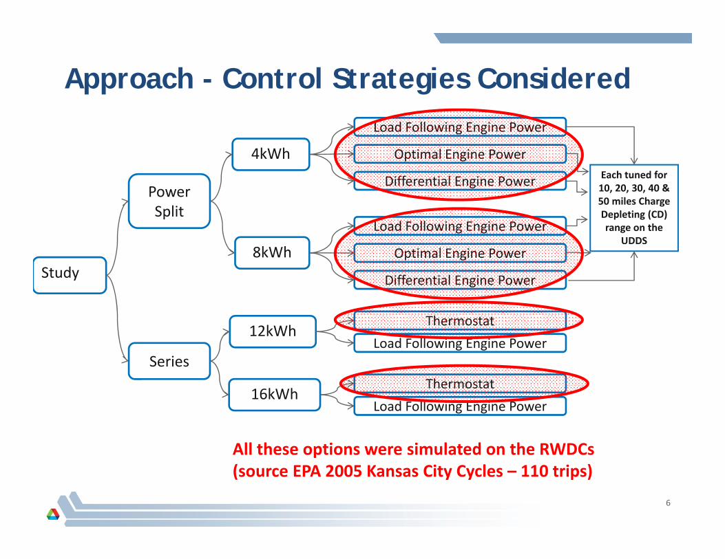
Differential Engine Power Strategy The engine is started when wheel power demand exceeds a certain 

threshold. 

It then provides the difference between the wheel power demand and the power threshold.

7

d1

Slide 7

d1 Shouldn't the Power threshold be the available max torque of the EM?dkarbowski, 3/19/2009

Load Following Strategy The engine is started when wheel power demand exceeds a certain 

threshold. 

It then provides the full wheel power, i.e. it is load following

8

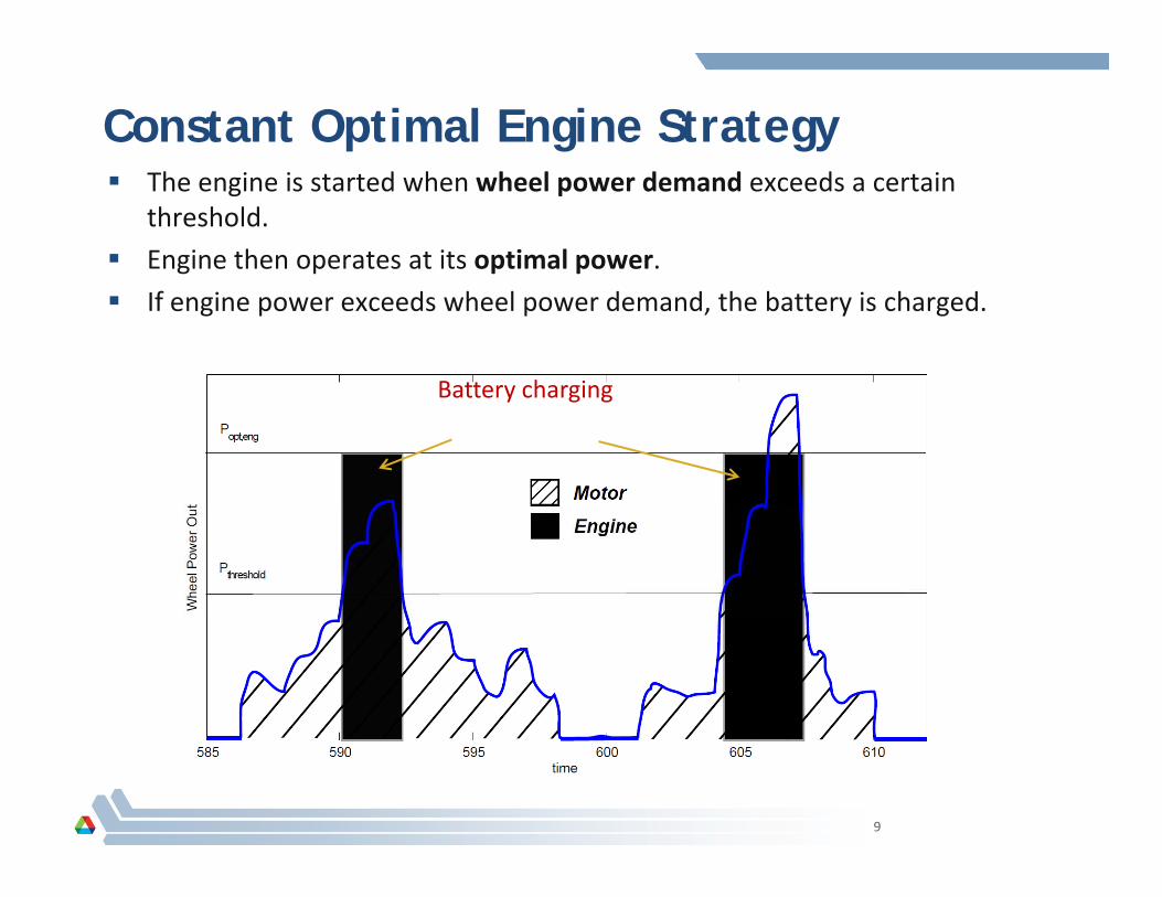
Constant Optimal Engine Strategy The engine is started when wheel power demand exceeds a certain 

threshold. 

Engine then operates at its optimal power. 

If engine power exceeds wheel power demand, the battery is charged.

Battery chargingBattery charging

9

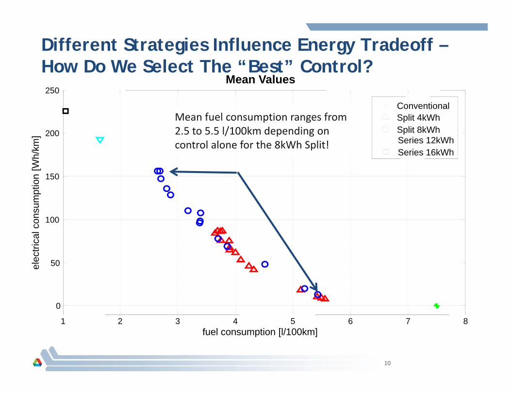
Different Strategies Influence Energy Tradeoff –How Do We Select The “Best” Control?250

Mean Values

Split 4kWhConventional

Mean fuel consumption ranges from 200

[Wh/

km] Series 12kWh

Series 16kWh

Split 8kWhp g

2.5 to 5.5 l/100km depending on control alone for the 8kWh Split!

100

150

onsu

mpt

ion

50

100

elec

trica

l co

1 2 3 4 5 6 7 8

0

10

1 2 3 4 5 6 7 8fuel consumption [l/100km]

Kernel Density Will be Used to Compare Control OptionsControl Options

40

Distribution Fuel ConsumptionConventional Vehicle

30

35

es

histogramkernel density estimation

20

25

of O

ccur

ence

10

15

Num

ber o

6 6.5 7 7.5 8 8.5 9 9.50

5

11

Fuel Consumption [liter/100km]

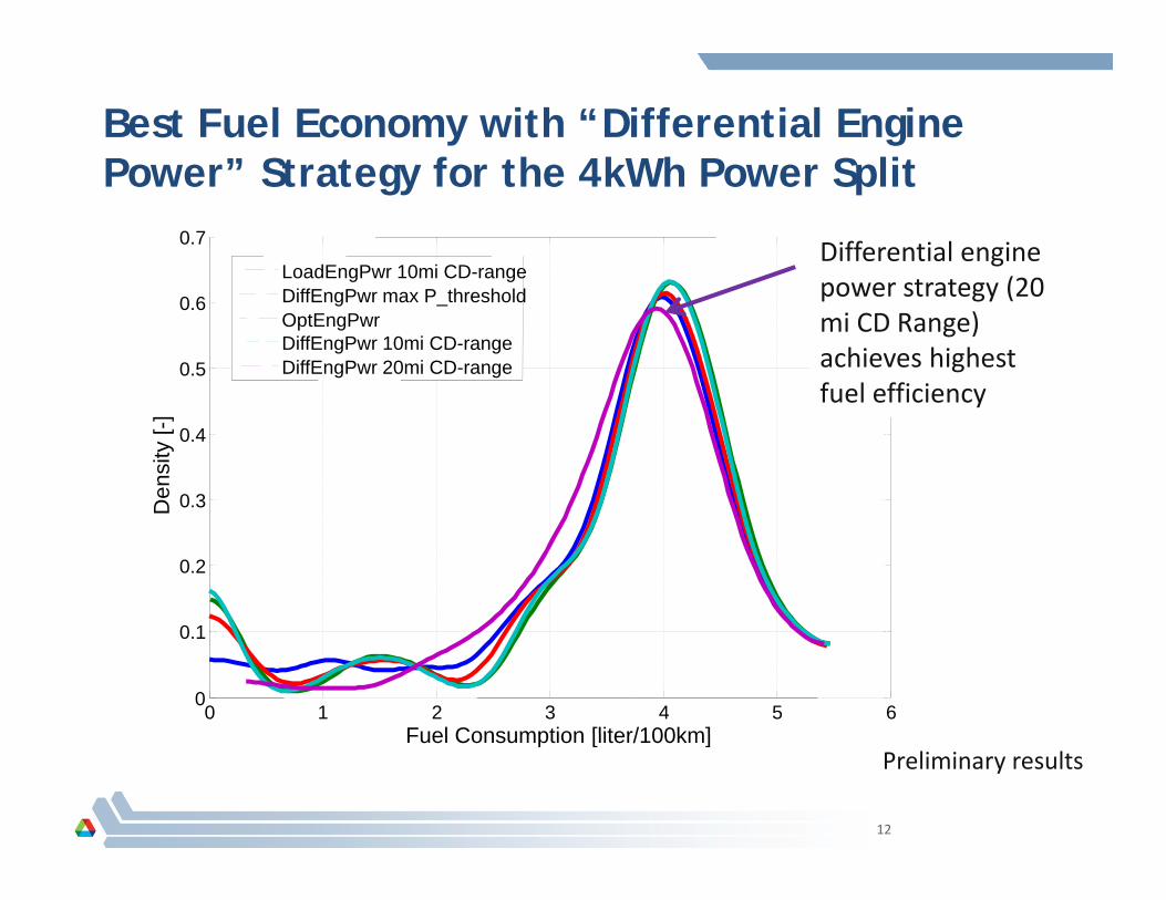
Best Fuel Economy with “Differential Engine Power” Strategy for the 4kWh Power SplitPower” Strategy for the 4kWh Power Split

0.7

LoadEngPwr 10mi CD-rangeDifferential engine 

t t (20

0.5

0.6g g

DiffEngPwr max P_thresholdOptEngPwrDiffEngPwr 10mi CD-rangeDiffEngPwr 20mi CD-range

power strategy (20 mi CD Range) achieves highest fuel efficiency

Performs best regarding fuel 0.3

0.4

Den

sity

[-]

fuel efficiency

g geconomy

0.2

0.3D

0 1 2 3 4 5 60

0.1

Fuel Consumption [liter/100km]

12

Fuel Consumption [liter/100km]Preliminary results

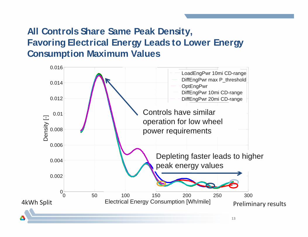
All Controls Share Same Peak Density, Favoring Electrical Energy Leads to Lower Energy

0.016LoadEngPwr 10mi CD-range

Favoring Electrical Energy Leads to Lower Energy Consumption Maximum Values

0.012

0.014

LoadEngPwr 10mi CD-rangeDiffEngPwr max P_thresholdOptEngPwrDiffEngPwr 10mi CD-rangeDiffEngPwr 20mi CD-range

0.008

0.01

nsity

[-] Controls have similar

operation for low wheel power requirements

0.004

0.006

De p q

Depleting faster leads to higher k l

0

0.002

peak energy values

0 50 100 150 200 250 3000

Electrical Energy Consumption [Wh/mile]

13

4kWh Split Preliminary results

Number of Engine Starts Clearly Distinguishes Control Strategies

0.35

0.4LoadEngPwr 10mi CD-rangeDiffEngPwr max P_thresholdOptEngPwrDiffE P 10 i CD

Strategies

0.25

0.3

[-]

DiffEngPwr 10mi CD-rangeDiffEngPwr 20mi CD-range

0.15

0.2

Den

sity

Performs best regarding # of engine starts

0.05

0.1

0 2 4 6 8 10 12 140

Number of starts per distance [#starts/mile]

14

4kWh Split Preliminary results

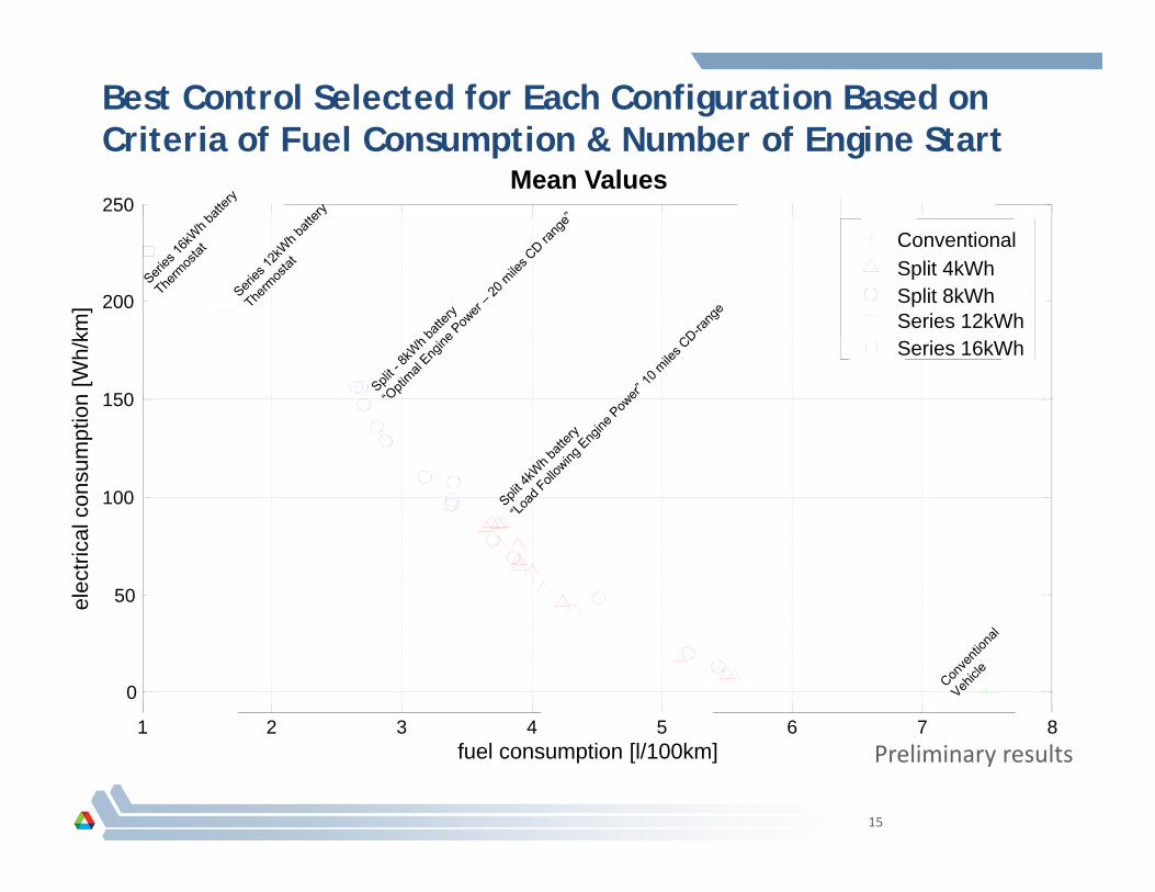
Best Control Selected for Each Configuration Based on Criteria of Fuel Consumption & Number of Engine Start

250Mean Values

Split 4kWhConventional

200

[Wh/

km]

Series 12kWhSeries 16kWh

pSplit 8kWh

100

150

onsu

mpt

ion

50

100

elec

trica

l co

1 2 3 4 5 6 7 8

0

15

1 2 3 4 5 6 7 8fuel consumption [l/100km] Preliminary results

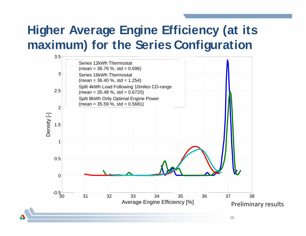
Higher Average Engine Efficiency (at its maximum) for the Series Configurationmaximum) for the Series Configuration

3

3.5Series 12kWh Thermostat(mean = 36.76 %, std = 0.696)S i 16kWh Th t t

2.5

3 Series 16kWh Thermostat(mean = 36.40 %, std = 1.254)Split 4kWh Load Following 10miles CD-range(mean = 35.48 %, std = 0.6720)Split 8kWh Only Optimal Engine Power(mean 35 59 % std 0 5681)

1.5

2

ensi

ty [-

]

(mean = 35.59 %, std = 0.5681)

0.5

1

D

0 5

0

16

30 31 32 33 34 35 36 37 38-0.5

Average Engine Efficiency [%] Preliminary results

Future Activities

Expand study to other Real World Drive Cycles (RWDC) –Source INLSource INL

Develop and test control strategies with trip recognition

Implement controls on hardware (if possible)Implement controls on hardware (if possible)

Understand differences with J1711 fuel efficiency results

17

Summary The analysis is only valid for the specific set of RWDC The analysis is only valid for the specific set of RWDC.

Several control strategies and set of parameters were evaluated on Real World Drive Cycles.y

Different controls were selected based on fuel efficiency and drive quality.

Control selected varies depending on the battery energy.– Load Following for 4kWh battery

– Optimum Engine for 8kWh batteryp g y

– Thermostat for 12 and 16 kWh battery

Impact of component operating conditions assessed

Preliminary comparison with J1711 shows fuel economy under evaluated

18

References D. Karbowski, “Fair Comparison of Powertrain Configurations for Plug‐In 

Hybrid Operation using Global Optimization”, SAE 2009‐01‐1334, SAE World Congress, April 2009

Rousseau, A. Pagerit, S., Gao, D. (Tennessee Tech University) , "Plug‐in hybrid electric vehicle control strategy parameter optimization", Journal of Asian Electric Vehicles, Volume 6 Number 2 December 2008, ISSN 1348‐3927

P. Sharer, A. Rousseau, D. Karbowski, S. Pagerit, “Plug‐in Hybrid Electric Vehicle Control Strategy: Comparison between EV and Charge‐Depleting Options”, SAE paper 2008‐01‐0460, SAE World Congress, Detroit (April 2008).

19

Additional Slides

20

Analysis of Vehicle Speed Traces at Different Levels

40Drive cycle

15

20

25

30

35

40

Spee

d (m

ph)

A hill is the portion of a cycle 

25Drive cycle

40Drive cycle

35Drive cycle

0 500 1000 1500 2000 2500 30000

5

10

15

Time (s)

between two stops

10

15

20

Spee

d (m

ph)

15

20

25

30

35Sp

eed

(mph

)

15

20

25

30

Spee

d (m

ph)

0 200 400 600 800 1000 12000

5

Time (s)0 500 1000 1500 2000 2500 30000

5

10

Time (s) 0 500 1000 1500 2000 25000

5

10

Time (s)

15

20

25

30

35

40

Speed (mph)

Drive cycle

21

0 1000 2000 3000 4000 5000 6000 70000

5

10

15

Time (s)

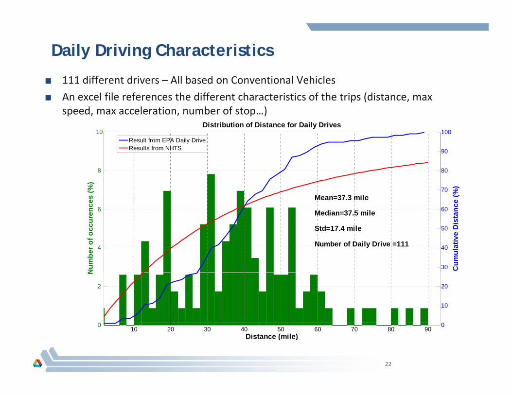
Daily Driving Characteristics

■ 111 different drivers – All based on Conventional Vehicles

■ An excel file references the different characteristics of the trips (distance, max speed, max acceleration, number of stop…)

Di t ib ti f Di t f D il D i

8

10

80

90

100Distribution of Distance for Daily Drives

Result from EPA Daily DriveResults from NHTS

6

uren

ces

(%)

60

70

stan

ce (%

)

Mean=37.3 mile

Median=37.5 mile

4

Num

ber o

f occ

u

30

40

50

Cum

ulat

ive

Di

Std=17.4 mile

Number of Daily Drive =111

2

N

10

20

22

0 10 20 30 40 50 60 70 80 90

0

Distance (mile)

Additional Characteristics of the Daily Driving20 100

Distribution of Max speed for Daily Drives40 100

Distribution of Mean acceleration positive for Daily Drives

12

16

20

ence

s (%

)

60

70

80

90

100

spee

d (%

)

Mean=72.3 mile/hMedian=72 mile/hStd=8.5 mile/h 24

32

40

ence

s (%

)

60

70

80

90

100

atio

n po

sitiv

e (%

)Mean=0.7 m/s2Median=0.7 m/s2Std=0.1 m/s2Number of Daily Drive =111

US06

US06

4

8

Num

ber o

f occ

ur

20

30

40

50

Cum

ulat

ive

Max

sStd 8.5 mile/hNumber of Daily Drive =111

8

16

Num

ber o

f occ

ure

20

30

40

50

ulat

ive

Mea

n ac

cele

ra

HWFET

LA92U

DDS

HWFET 

(0.16 m/s2)

UDDS LA92

US06

0 40 50 60 70 80 90 100 110 120

0

10

Max speed (mile/h)0

0.5 0.55 0.6 0.65 0.7 0.75 0.8 0.850

10

Cum

u

Mean acceleration positive (m/s2)

20 100Mean=33 4 mile/h

Distribution of Mean speed for Daily Drives30 100

Distribution of Mean deceleration for Daily Drives

12

16

cure

nces

(%)

60

70

80

90

an s

peed

(%)

Mean=33.4 mile/hMedian=33.5 mile/hStd=6.8 mile/hNumber of Daily Drive =111

18

24

cure

nces

(%)

60

70

80

90

dece

lera

tion

(%)

Mean=-0.8 m/s2

Median=-0.8 m/s2

Std=0.1 m/s2

Number of Daily Drive =111

HWFET

US06

US06

4

8

Num

ber o

f occ

10

20

30

40

50

Cum

ulat

ive

Mea

6

12

Num

ber o

f occ

20

30

40

50

Cum

ulat

ive

Mea

n dLA

92

UDDS HWFET 

(0.13 m/s2)

UDDS 

(0.48 m/s2)

LA92

23

0 20 25 30 35 40 45 50 55

0

10

Mean speed (mile/h)0 -1 -0.95 -0.9 -0.85 -0.8 -0.75 -0.7 -0.65 -0.6 -0.55 -0.5

0

10

Mean deceleration (m/s2)

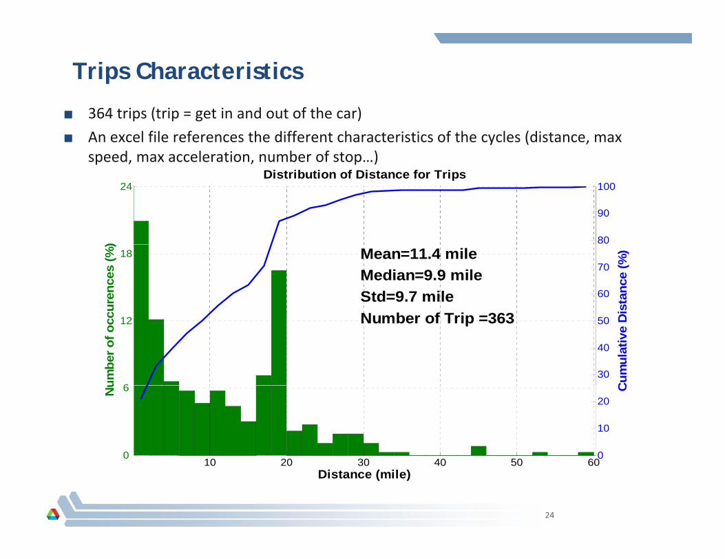
Trips Characteristics

■ 364 trips (trip = get in and out of the car)

■ An excel file references the different characteristics of the cycles (distance, max speed, max acceleration, number of stop…)

Distribution of Distance for Trips24

) 80

90

100Distribution of Distance for Trips

18

cure

nces

(%)

60

70

Dis

tanc

e (%

)Mean=11.4 mileMedian=9.9 mileStd=9.7 mileN b f T i 363

6

12

umbe

r of o

cc

30

40

50

Cum

ulat

ive

DNumber of Trip =363

0

6 Nu

0

10

20

C

24

0 10 20 30 40 50 60

0

Distance (mile)

Additional Characteristics of the Trips10 100

Distribution of Max speed for Trips 20 100Distribution of Mean acceleration for Trips

6

8

10

ence

s (%

)

60

70

80

90

100

peed

(%)

Mean=57.9 mile/hMedian=61.1 mile/h

Std=16.1 mile/hNumber of Trip =363

12

16

renc

es (%

)

60

70

80

90

ccel

erat

ion

(%)

Mean=0.4 m/s2Median=0.4 m/s2Std=0.1 m/s2

2

4

Num

ber o

f occ

ure

20

30

40

50

Cum

ulat

ive

Max

s

4

8

Num

ber o

f occ

u

20

30

40

50

Cum

ulat

ive

Mea

n acNumber of Trip =363

0 20 30 40 50 60 70 80 90 100

0

10

Max speed (mile/h)

0 0.1 0.2 0.3 0.4 0.5 0.6 0.7 0.8 0.9 1 1.1

0

10

C

Mean acceleration (m/s2)

10 100

Mean=28.5 mile/h

Distribution of Mean speed for Trips24

90

100Distribution of Mean deceleration for Trips

6

8

ccur

ence

s (%

)

50

60

70

80

90

ean

spee

d (%

)

Median=28.7 mile/h

Std=10.9 mile/h

Number of Trip =363

12

18

ccur

ence

s (%

)50

60

70

80

90

n de

cele

ratio

n (%

)

Mean=-0.5 m/s2Median=-0.4 m/s2Std=0.1 m/s2Number of Trip =363

2

4

Num

ber o

f oc

10

20

30

40

50

Cum

ulat

ive

M

6

12N

umbe

r of o

c

10

20

30

40

50

Cum

ulat

ive

Mea

nNumber of Trip 363

25

0 10 20 30 40 50 60

0

Mean speed (mile/h)0

-1.2 -1 -0.8 -0.6 -0.4 -0.2 00

Mean deceleration (m/s2)

Cycles Cross correlation Cross correlation

100150200

size

d

Distance vs. Max speed

Regression-50

0

P ess

harg

ing

er e

ach

cycl

e

100

200

Pes

s

disc

harg

ing

per e

ach

c

ycle

50100

P ess

Regression

50

100

Max

S

peed

0204060

Dist

ance

-100

Pch pe c

on

123

Max

ac

cele

ratio

n 0200040006000

Tim

e

0 81

e

tio

n

2040

60

Aver

age

spee

d

-4

-2

Max

de

cele

ratio

-1.2-1-0.8-0.6-0.4-0.2Average

0.20.40.6 0.8 1Average

20 40 60Average

-4 -2Max

1 2 3Max

0 200040006000Time

50 100Max

0 20 40 60Distance

-100 -50 0Pess

100 200Pess

50 100150200-1.2

-1-0.8-0.6-0.4-0.2

Pess sized

Aver

age

dece

lera

tion 0.2

0.40.60.8

Aver

age

acce

lera

t

26

decelerationaccelerationspeed decelerationaccelerationSpeedess

chargingper each cycle

essdischargingper each cycle

ess

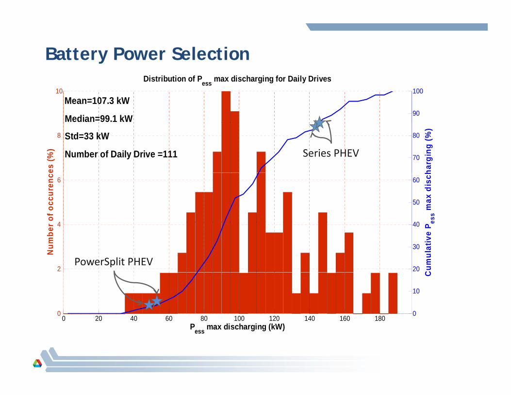
Battery Power Selection

10

90

100Mean=107.3 kW

Median=99.1 kW

Distribution of Pess max discharging for Daily Drives

8

es (%

)

70

80

harg

ing

(%)

Std=33 kW

Number of Daily Drive =111 Series PHEV

4

6

of o

ccur

ence

40

50

60

ess m

ax d

isch

2

4

Num

ber

20

30

40

Cum

ulat

ive

P e

PowerSplit PHEV

0 0 20 40 60 80 100 120 140 160 180

0

10

C

Pess max discharging (kW)

27

Di t ib ti f B tt E t f D il d i

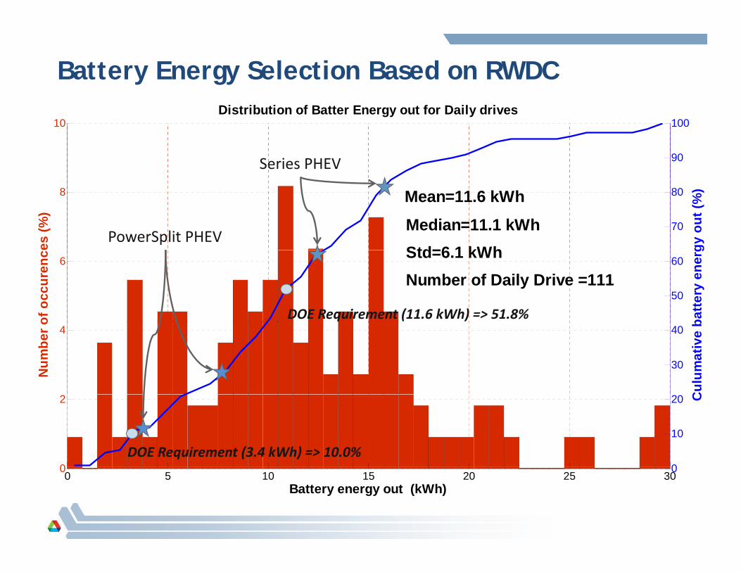
Battery Energy Selection Based on RWDC

10

90

100Distribution of Batter Energy out for Daily drives

Series PHEV

8

es (%

)

70

80

gy o

ut (%

)Mean=11.6 kWh

Median=11.1 kWhStd=6 1 kWh

PowerSplit PHEV6

of o

ccur

enc

50

60

batte

ry e

nergStd=6.1 kWh

Number of Daily Drive =111

DOE Requirement (11.6 kWh) => 51.8%4

Num

ber o

30

40

Cul

umat

ive

b

0

2

0

10

20 C

DOE Requirement (3.4 kWh) => 10.0%00 5 10 15 20 25 30

0

Battery energy out (kWh)

28

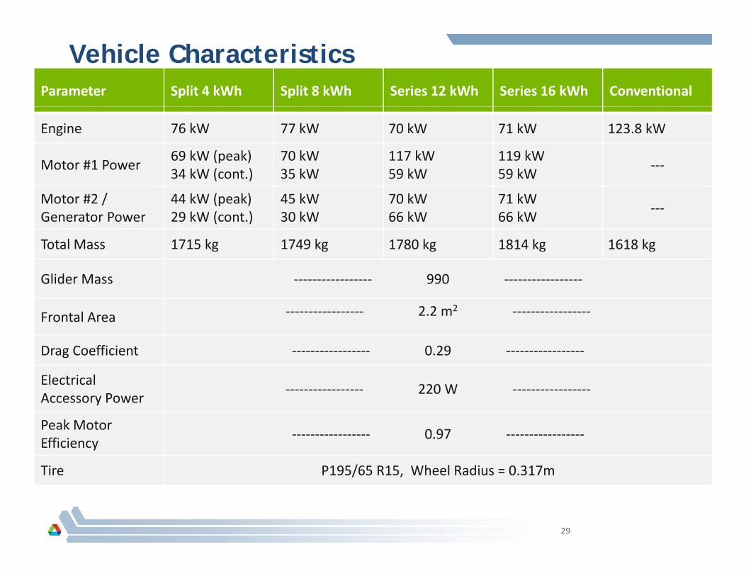
Vehicle CharacteristicsParameter Split 4 kWh Split 8 kWh Series 12 kWh Series 16 kWh Conventional

Engine 76 kW 77 kW 70 kW 71 kW 123.8 kW

Motor #1 Power69 kW (peak)34 kW (cont.)

70 kW35 kW

117 kW59 kW

119 kW59 kW

‐‐‐( )

Motor #2 /Generator Power

44 kW (peak)29 kW (cont.)

45 kW30 kW

70 kW66 kW

71 kW66 kW

‐‐‐

Total Mass 1715 kg 1749 kg 1780 kg 1814 kg  1618 kg

Glider Mass ‐‐‐‐‐‐‐‐‐‐‐‐‐‐‐‐‐ 990                ‐‐‐‐‐‐‐‐‐‐‐‐‐‐‐‐‐

Frontal Area ‐‐‐‐‐‐‐‐‐‐‐‐‐‐‐‐‐ 2.2 m2 ‐‐‐‐‐‐‐‐‐‐‐‐‐‐‐‐‐

Drag Coefficient ‐‐‐‐‐‐‐‐‐‐‐‐‐‐‐‐‐ 0.29                ‐‐‐‐‐‐‐‐‐‐‐‐‐‐‐‐‐

Electrical Accessory Power

‐‐‐‐‐‐‐‐‐‐‐‐‐‐‐‐‐ 220 W   ‐‐‐‐‐‐‐‐‐‐‐‐‐‐‐‐‐Accessory Power

Peak MotorEfficiency

‐‐‐‐‐‐‐‐‐‐‐‐‐‐‐‐‐ 0.97                ‐‐‐‐‐‐‐‐‐‐‐‐‐‐‐‐‐

Tire P195/65 R15 Wheel Radius = 0 317m

29

Tire P195/65 R15,  Wheel Radius = 0.317m