Embed Size (px)
Citation preview
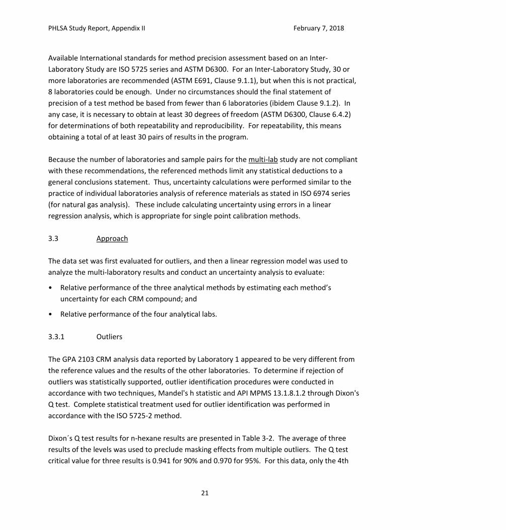
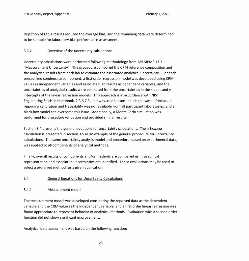
PHLSA Study Report, Appendix II February 7, 2018
i
PHLSA Study Final Report
Appendix II
Uncertainty Analysis
Table of Contents
List of Tables ................................................................................................................................... iii
List of Figures .................................................................................................................................. vi
Abbreviations, Acronyms, and Symbols ......................................................................................... ix
References .................................................................................................................................... xiii
1.0 Introduction. ....................................................................................................................... 1
2.0 Certified Reference Material. ............................................................................................. 2
2.1 Description of Uncertainty Sources .................................................................................... 4
2.2 Software Validation ............................................................................................................ 5
2.3 Input data for calculations .................................................................................................. 7
2.4 C6+ Molecular Weight Uncertainty ..................................................................................... 9
2.5 CRM and C6+ Specific Gravity Uncertainty Calculations .................................................. 16
2.6 Summary of CRM uncertainty calculations....................................................................... 19
3.0 Multi-laboratory study. ..................................................................................................... 20
3.1 Introduction ...................................................................................................................... 20
3.2 Background ....................................................................................................................... 20
3.3 Approach ........................................................................................................................... 21
3.4 General Equations for Uncertainty Calculations .............................................................. 23
3.5 Measurement Uncertainty of Multi-laboratory Study ..................................................... 29
3.6 Summary of Multi-Laboratory Study Findings .................................................................. 33
4.0 SPL Analytical Methods Evaluation. .................................................................................. 34
4.1 Introduction and Approach............................................................................................... 34
4.2 Summary of SPL Analytical Methods Uncertainty and Bias ............................................. 34
4.3 Weighted Bias ................................................................................................................... 38
4.4 GPA Method 2286 ............................................................................................................. 40
5.0 Sample Collection and Sample Handling Perturbation Studies. ....................................... 44
PHLSA Study Report, Appendix II February 7, 2018
ii
5.1 Sample Handling Perturbation Study ............................................................................... 44
5.2 Sample Collection Perturbation Study .............................................................................. 58
6.0 Process measurement. ..................................................................................................... 91
6.1 Introduction ...................................................................................................................... 91
6.2 Uncertainty of General Process Instrumentation ............................................................. 92
6.3 Coriolis Liquid Flow Meter .............................................................................................. 100
7.0 Uncertainty of Storage Tank Mass Balance and FGOR Measurements. ........................ 102
8.0 PSM/EOS FGOR Calculations Uncertainty Analysis. ....................................................... 103
8.1 Introduction .................................................................................................................... 103
8.2 Numerical Approximation Uncertainty Calculation ........................................................ 104
8.3 Monte Carlo Simulation .................................................................................................. 108
8.4 Summary of Results ........................................................................................................ 110
List of Tables ................................................................................................................................... iii
List of Figures ................................................................................................................................... v
Abbreviations, Acronyms, and Symbols ........................................................................................ vii
References ...................................................................................................................................... xi
PHLSA Study Report, Appendix II February 7, 2018
iii
List of Tables
Table 2-1. Molecular Weight and Uncertainty ISO 6976:2016 (E) .......................................... 7
Table 2-2. Elemental Molecular Weight and Uncertainty ISO 6976:2016 (E) ......................... 8
Table 2-3. Density and Uncertainty (NIST REFPROP) ............................................................... 8
Table 2-4. Cryoscope Readings for Repeatability Uncertainty Calculation ........................... 14
Table 2-5. Quality Control Toluene Samples ......................................................................... 18
Table 2-6 Input Variables for Specific Gravity of Toluene Standard Uncertainty Calculation18
Table 2-7. CRM 101259 Composition and Uncertainty Estimates ........................................ 19
Table 3-1. Number of Samples Analyzed for the Multi-laboratory Study ............................. 20
Table 3-2. Q-test for n-Hexane by GPA 2103 Average Values ............................................... 22
Table 3-3. R Code Calculation of Slope and Intercept for n-Hexane ..................................... 27
Table 3-4. GPA 2103 Analysis, n-Hexane Uncertainty ........................................................... 28
Table 3-5a. Multi-laboratory Study GPA 2103M Analysis Uncertainty (Lab 1 Outliers
Removed) .............................................................................................................. 29
Table 3-5b. Multi-laboratory Study GPA 2103M Analysis Uncertainty (Lab 1 Outliers
Included) ............................................................................................................. 30
Table 3-6. Multi-laboratory Study GPA 2186M Analysis Uncertainty ................................... 30
Table 3-7. Multi-laboratory Study Flash Liberation Analysis Uncertainty ............................. 31
Table 3-8. C10+ Specific Gravity and Molecular Weight Analyses Uncertainties.................. 31
Table 4-1. Summary of SPL Analytical Methods Uncertainty Estimates ............................... 35
Table 4-2. Summary of Analytical Methods Bias Estimates .................................................. 36
Table 4.3. Example Sample for Weighted Bias Calculation ................................................... 39
Table 4-4. General Method Bias ............................................................................................ 39
Table 4-5. GPA 2286 Analytical Range and Sample Composition (mole %) .......................... 40
Table 4-6. GPA 2261-13 Reproducibility ................................................................................ 42
Table 4-7. Gas Composition for Property Calculation Examples ........................................... 43
Table 4-8. Gas Properties from Composition ........................................................................ 43
Table 5-1 Laboratory Sample Handling Perturbations for CP and CV Cylinders .................. 44
PHLSA Study Report, Appendix II February 7, 2018
iv
Table 5-2. Calculated Vapor Pressures from Compositional Analysis ................................... 48
Table 5-3. Vapor Pressures Differences (Sample Analysis - CRM) ......................................... 49
Table 5-4. Effect on Vapor Pressures of Low Condition and High Condition Factors ........... 50
Table 5-5. Detailed Ruggedness Test Results ........................................................................ 51
Table 5-6. Summary of Results ............................................................................................. 53
Table 5-7 CP/CV Cylinders Paired Samples Comparison t-statistic Test Data, H0: davg = 0
(GPA 2103 Analysis) .............................................................................................. 66
Table 5-8. Goodness-of-fit Test Summary for Methane CP/CV Differences Data ................. 68
Table 5-9. Summary of Outlier Tests for Methane CP/CV Differences Data .......................... 69
Table 5-10. Goodness-of-fit Test Summary for Methane CP/CV Differences Data, with Outlier
Removed ................................................................................................................ 70
Table 5-11. Summary of WSRT for Methane CP/CV Differences Data .................................... 72
Table 5-12. CP/CV Cylinders Paired Samples Comparison t-statistic Test Data, H0: davg <
Analytical Uncertainty (GPA 2103 Analysis) .......................................................... 74
Table 5-13. Summary Statistics for CP/CV Cylinders Paired Samples Differences Data .......... 76
Table 5-14. Sight Glass/Sample Probe Paired Samples Comparison t-statistic Test Data, H0:
davg = 0 (GPA 2103 Analysis, CP and CV samples) ................................................. 87
Table 5-15. Sight Glass/Sample Probe Paired Samples Comparison t-statistic Test Data, H0:
davg = 0 (GPA 2103 Analysis, CP samples only) ...................................................... 88
Table 5-16. Sight Glass/Sample Probe Paired Samples Comparison t-statistic Test Data, H0:
davg = 0 (GPA 2103 Analysis, CV samples only) ...................................................... 89
Table 5-17. Sight Glass/Sample Probe Paired Samples Comparison Summary Statistics (GPA
2103 Analysis) ........................................................................................................ 90
Table 6-1. Process Measurement Standard Uncertainty Algorithm and Example Relative
Uncertainty at Half Full Scale ................................................................................ 95
Table 8-1. Tank One Foot from Bottom Pressure (TBP) ...................................................... 106
Table 8-2. Relative PSM/EOS FGOR Calculation Sensitivity Effect Determined by Numerical
Approximation ................................................................................................... 107
Table 8-3. Results of FGOR Uncertainty Calculations ......................................................... 111
Table 8-4. Results of Bubble Point Pressure Uncertainty Calculations .............................. 111
PHLSA Study Report, Appendix II February 7, 2018
v
Table 8-5. Results of Shrinkage Factor Uncertainty Calculations ....................................... 111
PHLSA Study Report, Appendix II February 7, 2018
vi
List of Figures
Figure 2-1 CRM sources of uncertainty. Rounded squares boxes represent type B
uncertainties. .......................................................................................................... 3
Figure 2-2 Sources of uncertainty for molecular weight measurements .............................. 11
Figure 3-1 Mandel's statistic for laboratories 1, 2 and 3. n-Hexane by GPA 2103 ................ 22
Figure 3-2 GPA 2103 n-Hexane data with outliers ................................................................. 22
Figure 3-3 GPA 2103 n-Hexane data after removal of removal of outliers ........................... 23
Figure 3-4 Multi-laboratory study analytical method uncertainty analysis results (%U for
analytes) ................................................................................................................ 32
Figure 4-1. SPL study analytical method uncertainty analysis results (%U for analytes)........ 37
Figure 5-1. Half normal plot of effects over vapor pressure .................................................. 50
Figure 5-2. Half normal plot of effects over Carbon Dioxide .................................................. 53
Figure 5-3. Half normal plot of effects over Nitrogen ............................................................ 54
Figure 5-4. Half normal plot of effects over Methane ............................................................ 54
Figure 5-5. Half normal plot of effects over Ethane ............................................................... 54
Figure 5-6. Half normal plot of effects over Propane ............................................................. 55
Figure 5-7. Half normal plot of effects over i-butane ............................................................. 55
Figure 5-8. Half normal plot of effects over n-Butane ............................................................ 56
Figure 5-9. Half normal plot of effects over i-Pentane ........................................................... 56
Figure 5-10. Half normal plot of effects over n-Pentane .......................................................... 57
Figure 5-11. Half normal plot of effects over Hexanes plus ..................................................... 57
Figure 5-12. Half normal plot of effects over Vapor pressure .................................................. 57
Figure 5-13. Histogram of the CP/CV differences data for methane ....................................... 67
Figure 5-14. Histogram of the CP/CV differences data for methane, with outlier removed ... 70
Figure 5-15. Impact of sample collection initiation time on PBP/PSC ......................................... 77
Figure 5-16. Impact of sample collection initiation time on pressurized condensate methane
concentration ........................................................................................................ 78
Figure 5-17. Impact of sample collection rate on PBP/PSC, Low-, Mid-, and High-Pressure well
cycles .................................................................................................................... 79
PHLSA Study Report, Appendix II February 7, 2018
vii
Figure 5-18. Impact of sample collection rate on PBP/PSC, Mid-Pressure well cycles 80
Figure 5-19. Impact of sample collection rate on condensate concentrations of CO2 and CH4 82
Figure 5-20. Impact of sample collection rate on condensate concentrations of C10+. 82
Figure 5-21. Impact of sample collection rate on condensate C10+ specific gravity 83
Figure 5-22. Impact of separator temperature on PBP/PSC 83
Figure 5-23. Impact of separator temperature on PBP. 84
Figure 5-24. Impact of separator temperature on CO2 and methane 84
Figure 5-25. Impact of sample collection location on PBP/PSC 86
Figure 8-1. Relative PSM/EOS FGOR calculation sensitivity effect determined by numerical
approximation 108
Figure 8-2. Monte Carlo simulation sensitivity study 110
PHLSA Study Report, Appendix II February 7, 2018
viii
Abbreviations, Acronyms, and Symbols
a Slope constant of first order regression (dimensionless)
b Ordinate to origin or intercept constant of first order regression (dimensionless)
API American Petroleum Institute
ASTM American Society for Testing and Materials
BAM Bundesanstalt für Materialforschung
bbl barrel
BTEX benzene + toluene + ethyl benzene + xylenes
BIPM Bureau International des Poids et Measures
Bz Weight of Benzene for Cryoscopy Analysis (g)
C1 methane
CH4 methane
C5 pentanes
C6+ hexanes and heavier hydrocarbons
C7+ heptanes and heavier hydrocarbons
C8+ octanes and heavier hydrocarbons
C10+ decanes and heavier hydrocarbons
ci Sensitivity coefficient
CI confidence interval
CO2 carbon dioxide
CP constant pressure
CRM Certified Reference Material
Cv Certified value of component for multi-laboratory study (regression dependent variable)
CV constant volume
D Knob adjustment of cryoscope
d density (g/mL)
DoF degrees of freedom
°F degrees Fahrenheit
FGOR flash gas-to-oil ratio
g gram
G relative density
GC gas chromatography
PHLSA Study Report, Appendix II February 7, 2018
ix
gmol gram-mole
GPA Gas Processors Association
GUM Guide to the expression of Uncertainty in Measurement
HP High pressure (well cycle)
IPT initial pressure test
ISO International Organization for Standardization
JCGM Joint Committee for Guides in Metrology
K Kelvin
k Number of data sets with different n elements
%L Component liquid volume percent (% liquid)
L Cryoscope reading of an unknown sample (dimensionless)
lb pound
LP Low pressure (well cycle)
LV% liquid volume percent
mi Component mass in 1 g of CRM (mass fraction) (g)
min minute
ml milli-liter
MW Molecular Weight (g/gmol)
MPMS Manual of Petroleum Measurement Standards
MWs Standard Molecular Weight (128.22 for n-Nonane) (g/gmol)
n Total number of elements or components of a data set
N2 nitrogen
NGLs natural gas liquids
NIST National Institute of Standards and Technology
NPL National Physical Laboratory
OPC operational performance check
PBP bubble point pressure
Psep Separator pressure
PSC Separator pressure during pressurized hydrocarbon sample collection
psia pounds per square inch absolute
psig pounds per square inch gauge
PSM/EOS process simulation modeling/ equation of state
PHLSA Study Report, Appendix II February 7, 2018
x
Ptank tank pressure
PVT pressure-volume-temperature
R Cryoscope reading for n-nonane
R ideal gas constant
R correlation coefficient (e.g., for linear regression equation)
Rv Reported value in multi-laboratory study, regression independent variable
s Standard deviation
scf standard cubic feet
sp Pooled standard deviation
seff Estimated standard deviation of test result
Sd Sample Standard Deviation
SW Sample weight for Cryoscopy Analysis (g)
SG Specific gravity at 60 °F/60 °F (dimensionless)
SHP summer high-pressure
SLP summer low-pressure
SMP summer mid-pressure
SPL Southern Petroleum Laboratories
SWs Weight of standard (n-Nonane) for Cryoscopy Analysis (g)
t Critical value of t distribution (i.e., for n-1 degrees of freedom)
TCD thermal conductivity detector
Tsep Separator temperature, typically during pressurized hydrocarbon sample collection
Ttank tank temperature
u Standard uncertainty (units of related variable)
U Expanded uncertainty (units of related variable)
%u Relative standard uncertainty (%)
%U Relative expanded uncertainty (%)
UK United Kingdom
WMP winter mid-pressure
wt% weight percent
WSRT Wilconxan Sign-Rank Test
Z compressibility factor
PHLSA Study Report, Appendix II February 7, 2018
xi
% percent
Δ difference or change
α significance level, is the probability of rejecting the null hypothesis when it is true
Density at 60 °F (g/mL)
i Density of component i at 60 °F (g/mL)
w Density of water at 60 °FD, 0.999017 (g/mL)
PHLSA Study Report, Appendix II February 7, 2018
xii
References.
1. API Manual of Petroleum Measurement Standards Chapter 13—Statistical Aspects of Measuring and
Sampling Section 1—Statistical Concepts and Procedures in Measurements reaffirmed, March 2016.
2. API Manual of Petroleum Measurement Standards Chapter 13.3 —Measurement Uncertainty. First Ed.
May 2016.
3. ASTM D6300 − 16 Standard Practice for Determination of Precision and Bias Data for Use in Test
Methods for Petroleum Products and Lubricants
4. ASTM E691 − 16 “Standard Practice for Conducting an Inter-laboratory Study to Determine the
Precision of a Test Method”
5. JCGM 100:2008. GUM 1995 with minor corrections. Evaluation of measurement data — Guide to the
expression of uncertainty in measurement.
6. JCGM 101:2008 Evaluation of measurement data — Supplement 1 to the “Guide to the expression of
uncertainty in measurement” — Propagation of distributions using a Monte Carlo method
7. ISO 5725-2. Accuracy (trueness and precision) of measurement methods and results - Part 2: Basic
method for the determination of repeatability and reproducibility of a standard measurement method
8. ISO/TS 29041 (E) Gas mixtures - Gravimetric preparation - Mastering correlations in composition.
9. ISO 6142-1 (E) Gas analysis - Preparation of calibration gas mixtures - Part 1: Gravimetric method for
Class I mixtures.
10. ISO 14912 Gas analysis -- Conversion of gas mixture composition data
11. ISO 6974 - 1 Natural gas - Determination of composition and associated uncertainty by gas
chromatography - Part 1: General guidelines and calculation of the composition.
12. ISO 6974-2 Natural gas - Determination of composition and associated uncertainty by gas
chromatography - Part 2: Uncertainty calculations.
13. ISO 6976:2016 Natural gas - Calculation of calorific values, density, relative density and Wobbe Index
from composition.
14. ISO 80000-1 First edition 2009-11-15 Quantities and units Part 1: General
15. GPA Standard 2261-13. Analysis for Natural Gas and Similar Gaseous Mixtures by Gas Chromatography.
16. GPA Midstream Standard 2145-16. Table of Physical Properties for Hydrocarbons and Other
Compounds of Interest to the Natural Gas and Natural Gas Liquids Industries.
17. GPA Standard 2103-03 “Tentative Method for the Analysis of Natural Gas Condensate Mixtures Containing Nitrogen and Carbon Dioxide by Gas Chromatography”
PHLSA Study Report, Appendix II February 7, 2018
xiii
18. GPA Standard 2177-13 “Analysis of Natural Gas Liquid Mixtures Containing Nitrogen And Carbon Dioxide By Gas Chromatography“
19. GPA 2186-14“Tentative Method for the Extended Analysis of Hydrocarbon Liquid Mixtures Containing Nitrogen and Carbon Dioxide by Temperature Programmed Gas Chromatography”
PHLSA Study Report, Appendix II February 7, 2018
1
1. Introduction
Many variables impact estimates of flash gas generated in atmospheric oil storage tanks and
contribute to complex uncertainty calculations. Integrating data from multiple components,
procedures, operators, environmental conditions, instruments, maintenance and calibrations is
required to estimate the uncertainty of oil tank flash gas generation.
Assessing the influence of each contributing parameter to a measured or calculated result is
critical and necessary for confidence in the estimated uncertainty of the result. This
assessment must be accomplished by detailed procedures based upon recognized practices or
standards. Detailed documentation of data sources such as calibration reports, experimental
data and other published sources contribute to support trustworthiness of results.
API MPMS (American Petroleum Institute Manual of Petroleum Measurement Standards)
Chapters 13.1 and 13.3 were the primary guidelines for calculating uncertainty estimates for
the PLHSA project. The latter is based upon the 2008 edition of the International Organization
of Standards (ISO) Guide to the Expression of Uncertainty in Measurement (GUM)-JCGM
100:2008. This ISO document was developed as guide for writers of technical standards.
For some critical measurement components, such as chromatographic analytical methods or
Certified Reference Materials preparation, selected ASTM and ISO standards were determined
to be more appropriate for uncertainty estimate calculations than the API general standards.
In some cases, critical thinking, working group consensus, and professional judgement were
used to discuss and agree upon appropriate uncertainty estimate approaches. This report
includes the following sections that document the approach and results for primary uncertainty
estimates.
2.0 Preparation of Certified Reference Materials
3.0 Multi-laboratory Study
4.0 SPL Analytical Methods Evaluation
5.0 Sample Handling and Sample Collection Perturbation Studies
6.0 Process Measurement
7.0 Operational Performance Checks
8.0 Storage Tank Mass Balance and FGOR Measurements
9.0 PSM/EOS FGOR Calculations Uncertainty Analysis
PHLSA Study Report, Appendix II February 7, 2018
2
The O&G production facility used for this testing produces HC liquid that is classified as
condensate, and the terms HC liquid, condensate, and oil are used interchangeably in this
document.
2. Certified Reference Material
Supporting data and calculations for the information presented in this section can be found in
Annex 1.
Condensate Certified Reference Materials (CRM) were prepared in accordance with common
American industry practices and gravimetrically blended from high purity feedstocks of C1 – C5
hydrocarbons and characterized heavy ends (depentanized C6+) condensate obtained from the
test site storage tank. There were two target CRM compositions (i.e., “CRM1” and “CRM2”),
and about 30 CRM1 sample cylinders were prepared and about 30 CRM2 sample cylinders were
prepared.
CRM composition confirmation and associated uncertainty calculations were performed
applying API Chapter 13.3 and ISO International Standards ISO/TS 29041, ISO 6142-1 and ISO
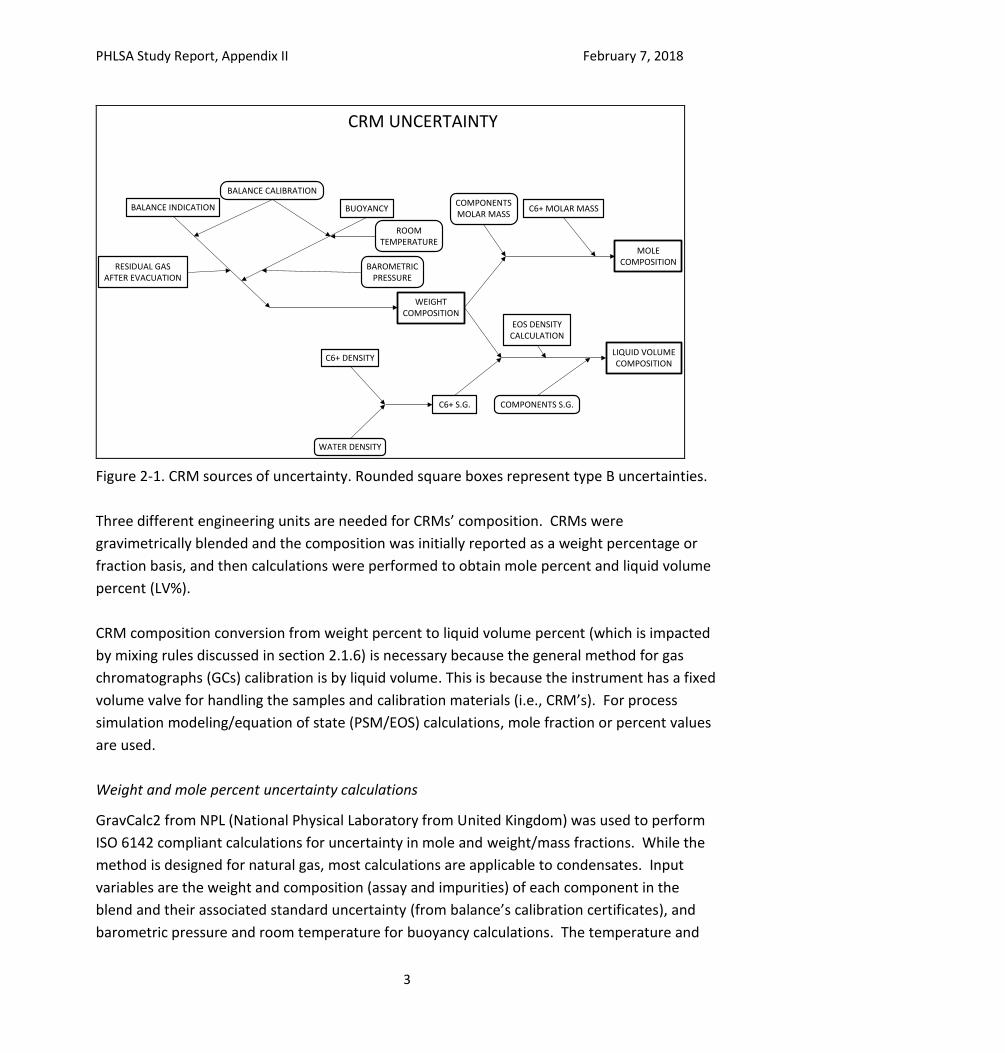
14912. Sources of uncertainty identified through these standards are schematically presented
in Figure 1-1 and include:
Feedstocks purity;
Balance linearity, minimum division, repeatability, and bias;
Buoyancy;
Published values of component molecular weights and densities;
C6+ fraction density and specific gravity; and
Other sources: vacuum residues, cylinder expansion by pressure, volume shrinkage for
liquid volume units.
PHLSA Study Report, Appendix II February 7, 2018
3
CRM UNCERTAINTY
WATER DENSITY
C6+ DENSITY
COMPONENTS S.G.
LIQUID VOLUMECOMPOSITION
C6+ S.G.
EOS DENSITYCALCULATION
BALANCE INDICATION
RESIDUAL GASAFTER EVACUATION
BUOYANCY
WEIGHTCOMPOSITION
BALANCE CALIBRATION
ROOMTEMPERATURE
BAROMETRIC PRESSURE
MOLECOMPOSITION
COMPONENTSMOLAR MASS
C6+ MOLAR MASS
Figure 2-1. CRM sources of uncertainty. Rounded square boxes represent type B uncertainties.
Three different engineering units are needed for CRMs’ composition. CRMs were
gravimetrically blended and the composition was initially reported as a weight percentage or
fraction basis, and then calculations were performed to obtain mole percent and liquid volume
percent (LV%).
CRM composition conversion from weight percent to liquid volume percent (which is impacted
by mixing rules discussed in section 2.1.6) is necessary because the general method for gas
chromatographs (GCs) calibration is by liquid volume. This is because the instrument has a fixed
volume valve for handling the samples and calibration materials (i.e., CRM’s). For process
simulation modeling/equation of state (PSM/EOS) calculations, mole fraction or percent values
are used.
Weight and mole percent uncertainty calculations
GravCalc2 from NPL (National Physical Laboratory from United Kingdom) was used to perform
ISO 6142 compliant calculations for uncertainty in mole and weight/mass fractions. While the
method is designed for natural gas, most calculations are applicable to condensates. Input
variables are the weight and composition (assay and impurities) of each component in the
blend and their associated standard uncertainty (from balance’s calibration certificates), and
barometric pressure and room temperature for buoyancy calculations. The temperature and
PHLSA Study Report, Appendix II February 7, 2018
4
pressure were obtained from the databases of meteorological stations close to the Reference
Materials Producer laboratory. A detailed explanation of the calculation model can be found in
ISO 6142.
Liquid volume uncertainty calculations
In absence of an International Standard for liquid volume uncertainty calculations, these
calculations were performed following API 13.3 and BIPM GUM guidelines JCGM 100:2008.
Densities from Refprop by National Institute of Standards and Technology (NIST), rather than
GPA 2145, were used. Refprop provides a generic uncertainty for density of around 0.02%, or
higher (up to 0.2%), for almost all the components in the CRMs. Differences in densities
between the two data sources (i.e., Refprop and GPA 2145) are small compared to related
uncertainty levels. Refer to Annex 2 for input data (type B).
2.1 Description of Uncertainty Sources
2.1.1 Weighing
The weighing process uncertainty considers the weight without tare zeroing uncertainty and
uncertainty at range of balance. The weight amount of substance is the weight of substance
plus vessel minus the tared vessel weight. The uncertainty of the net weight measurement is
approximately 40% (square root of 2 minus 1) greater than the balance uncertainty because the
mathematical operation includes two similar weight readings.
The uncertainty contribution from the balance is around 0.001 %, and the balance uncertainty
provides a very low contribution to the CRM uncertainty.
2.1.2 Buoyancy
Buoyancy, which accounts for the air displaced by the weighing vessel, is a variable for high
accuracy weighing. Even when the buoyancy correction is almost cancelled in net weight
calculations, its effect on uncertainty is not cancelled and it must be included in uncertainty
calculations. The contribution of buoyancy is only a small fraction of the overall weight
uncertainty.
PHLSA Study Report, Appendix II February 7, 2018
5
2.1.3 Molecular weight
The contribution of the C1 – C5 feedstocks molecular weight uncertainties to the overall CRM
molecular weight uncertainty is very small. The feedstocks molecular weight uncertainties
result from impurities and associated uncertainties of published molecular weights of
components. For CRM components molecular weights, ISO 6976-2016 data are used instead of
GPA 2145 because the ISO method includes uncertainties for molecular weights.
The C6+ fraction molecular weight was obtained from cryoscopy analysis prior to mixing with
the lighter components. Cryoscope molecular weight measurements have a relative
uncertainty of approximately 0.3%, and this value is the greatest contribution to the CRM mole
composition uncertainty. It is two orders of magnitude larger than uncertainties obtained from
molecular weight tables for the C1 – C5 feedstocks. The molecular weight by cryoscopy
uncertainty calculation is detailed in Section 2.4.
2.1.4 C6+ Density
Densities of C1 – C5 feedstocks components were obtained from Refprop. The C6+ fraction
density and specific gravity were determined by an oscillating tube method (i.e., densitometer)
with an ASTM D4052 compliant procedure. Repeatability of this method is around 0.1 %, and a
relative uncertainty obtained from Toluene quality control samples was used to estimate
sample uncertainties. An example detailed calculation can be found in Section 2.5.
2.1.5 Other minor sources
Uncertainty calculations included additional sources such as vacuum residues and cylinder
expansion by effect of pressure. These were considered negligible.
2.2 Software Validation
Even though the software used for uncertainty calculations are from trusted sources, the
calculations were validated using example input and output data from ISO 6142.
2.2.1 GravCalc2 (version 2.3.0), by NPL (National Physical laboratory, UK National
Metrology Institute) calculates mole fractions and associated uncertainties for mixtures of
gases prepared gravimetrically from known data of added mass, relative molecular mass of
each component, and the purity of the components based upon ISO 6142. The software was
validated using an example from Annex B of ISO 6142.
PHLSA Study Report, Appendix II February 7, 2018
6
2.2.2 CONVERT (version 1.0) by BAM (Bundesanstalt für Materialforschung und -
prüfung, German National Metrology Institute) was used to calculate uncertainties associated
with weight to mole percent conversions, including correlation matrix calculation of molecular
weight components updated to latest ISO 6976 version, and uncertainty of weight percent
values. CONVERT is compliant with ISO 14912, furthermore, this software is indicated in the
standard. Results of CONVERT were validated with examples of Annex D of ISO 14912.
2.2.3 The uncertainties of the CRM mass fractions (i.e., weight percent) were directly
calculated as described below. Converting the CRM weight percent values to mole % and LV%
required application of unit conversion constants. Calculating the uncertainty in the CRM mole
% and LV% values requires consideration of the uncertainty in the conversion factors. An Excel
calculation for liquid volume conversions and associated uncertainty calculations was
developed by Movilab and validated by confirmation of the same model with GUMsim 2.0.0
from Quodata.
PHLSA Study Report, Appendix II February 7, 2018
7
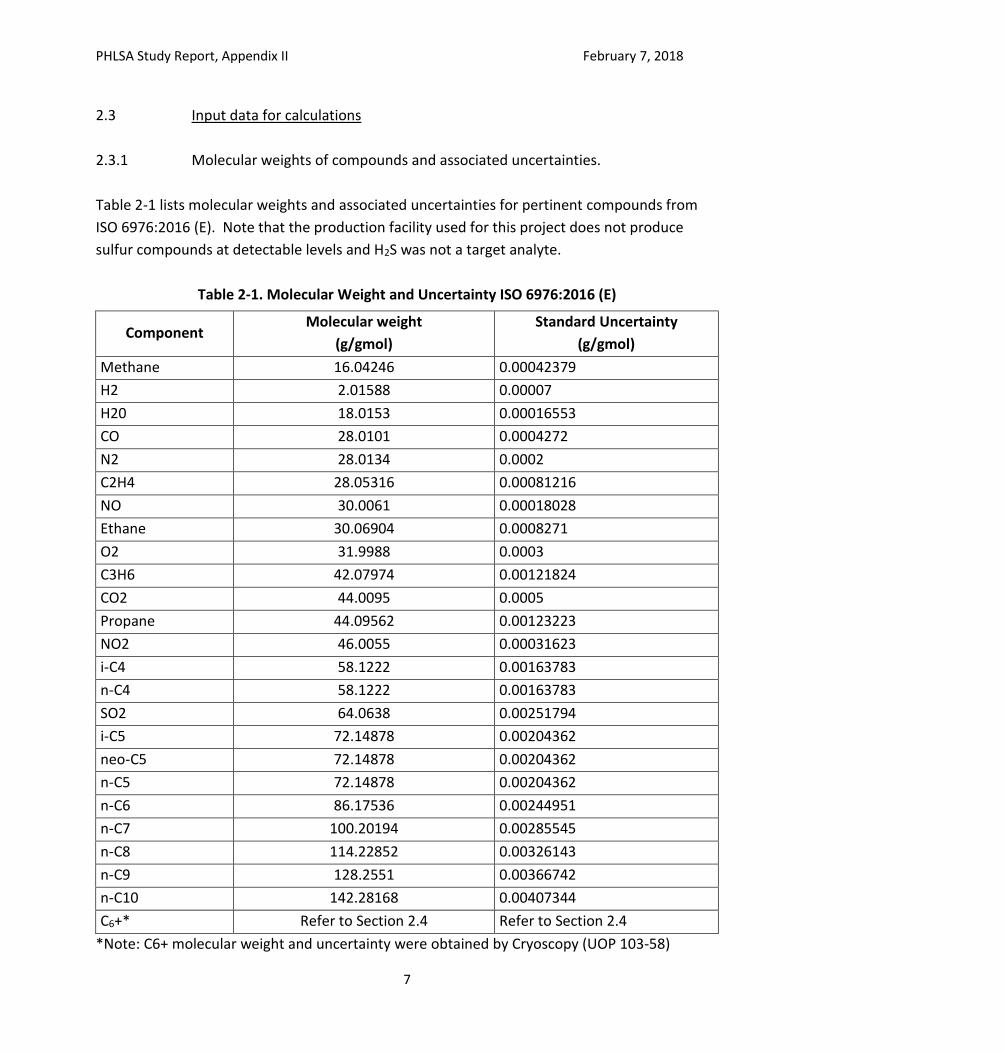
2.3 Input data for calculations
2.3.1 Molecular weights of compounds and associated uncertainties.
Table 2-1 lists molecular weights and associated uncertainties for pertinent compounds from
ISO 6976:2016 (E). Note that the production facility used for this project does not produce
sulfur compounds at detectable levels and H2S was not a target analyte.
Table 2-1. Molecular Weight and Uncertainty ISO 6976:2016 (E)
Component Molecular weight
(g/gmol)
Standard Uncertainty
(g/gmol)
Methane 16.04246 0.00042379
H2 2.01588 0.00007
H20 18.0153 0.00016553
CO 28.0101 0.0004272
N2 28.0134 0.0002
C2H4 28.05316 0.00081216
NO 30.0061 0.00018028
Ethane 30.06904 0.0008271
O2 31.9988 0.0003
C3H6 42.07974 0.00121824
CO2 44.0095 0.0005
Propane 44.09562 0.00123223
NO2 46.0055 0.00031623
i-C4 58.1222 0.00163783
n-C4 58.1222 0.00163783
SO2 64.0638 0.00251794
i-C5 72.14878 0.00204362
neo-C5 72.14878 0.00204362
n-C5 72.14878 0.00204362
n-C6 86.17536 0.00244951
n-C7 100.20194 0.00285545
n-C8 114.22852 0.00326143
n-C9 128.2551 0.00366742
n-C10 142.28168 0.00407344
C6+* Refer to Section 2.4 Refer to Section 2.4
*Note: C6+ molecular weight and uncertainty were obtained by Cryoscopy (UOP 103-58)
PHLSA Study Report, Appendix II February 7, 2018
8
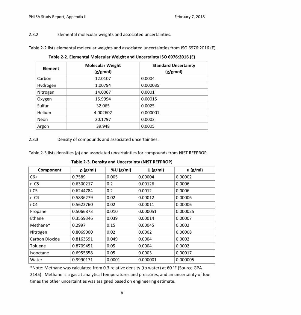
2.3.2 Elemental molecular weights and associated uncertainties.
Table 2-2 lists elemental molecular weights and associated uncertainties from ISO 6976:2016 (E).
Table 2-2. Elemental Molecular Weight and Uncertainty ISO 6976:2016 (E)
Element Molecular Weight
(g/gmol)
Standard Uncertainty
(g/gmol)
Carbon 12.0107 0.0004
Hydrogen 1.00794 0.000035
Nitrogen 14.0067 0.0001
Oxygen 15.9994 0.00015
Sulfur 32.065 0.0025
Helium 4.002602 0.000001
Neon 20.1797 0.0003
Argon 39.948 0.0005
2.3.3 Density of compounds and associated uncertainties.
Table 2-3 lists densities (ρ) and associated uncertainties for compounds from NIST REFPROP.
Table 2-3. Density and Uncertainty (NIST REFPROP)
Component ρ (g/ml) %U (g/ml) U (g/ml) u (g/ml)
C6+ 0.7589 0.005 0.00004 0.00002
n-C5 0.6300217 0.2 0.00126 0.0006
i-C5 0.6244784 0.2 0.0012 0.0006
n-C4 0.5836279 0.02 0.00012 0.00006
i-C4 0.5622760 0.02 0.00011 0.00006
Propane 0.5066873 0.010 0.000051 0.000025
Ethane 0.3559346 0.039 0.00014 0.00007
Methane* 0.2997 0.15 0.00045 0.0002
Nitrogen 0.8069000 0.02 0.0002 0.00008
Carbon Dioxide 0.8163591 0.049 0.0004 0.0002
Toluene 0.8709451 0.05 0.0004 0.0002
Isooctane 0.6955658 0.05 0.0003 0.00017
Water 0.9990171 0.0001 0.000001 0.000005
*Note: Methane was calculated from 0.3 relative density (to water) at 60 °F (Source GPA
2145). Methane is a gas at analytical temperatures and pressures, and an uncertainty of four
times the other uncertainties was assigned based on engineering estimate.
PHLSA Study Report, Appendix II February 7, 2018
9
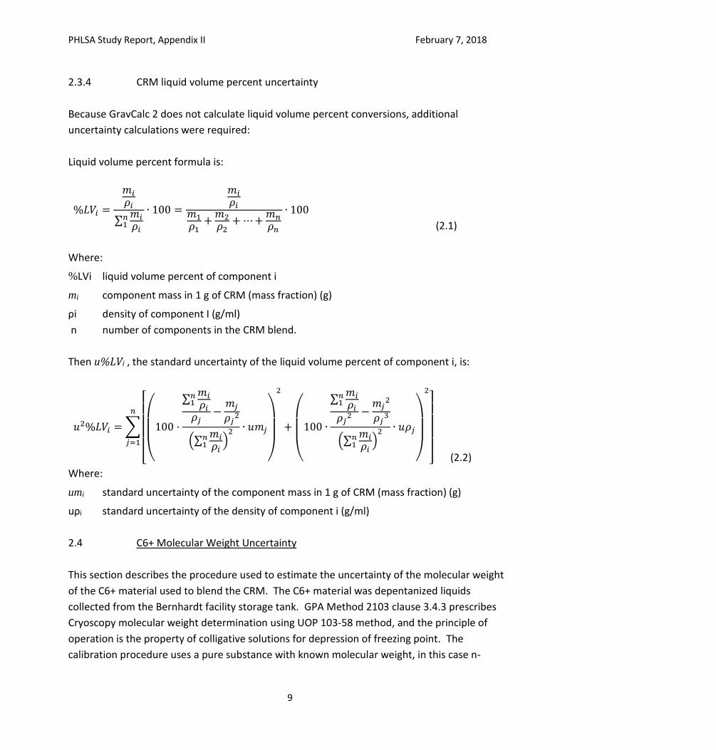
2.3.4 CRM liquid volume percent uncertainty
Because GravCalc 2 does not calculate liquid volume percent conversions, additional
uncertainty calculations were required:
Liquid volume percent formula is:
%𝐿𝑉𝑖 =
𝑚𝑖
𝜌𝑖
∑𝑚𝑖
𝜌𝑖
𝑛1
∙ 100 =
𝑚𝑖
𝜌𝑖𝑚1
𝜌1+
𝑚2
𝜌2+ ⋯+
𝑚𝑛
𝜌𝑛
∙ 100
(2.1)
Where:
%LVi liquid volume percent of component i
mi component mass in 1 g of CRM (mass fraction) (g)
ρi density of component I (g/ml)
n number of components in the CRM blend.
Then u%LVi , the standard uncertainty of the liquid volume percent of component i, is:
𝑢2%𝐿𝑉𝑖 = ∑
[
(
100 ·
∑𝑚𝑖
𝜌𝑖
𝑛1
𝜌𝑗−
𝑚𝑗
𝜌𝑗2
(∑𝑚𝑖
𝜌𝑖
𝑛1 )
2 ∙ 𝑢𝑚𝑗
)
2
+
(
100 ∙
∑𝑚𝑖
𝜌𝑖
𝑛1
𝜌𝑗2 −
𝑚𝑗2
𝜌𝑗3
(∑𝑚𝑖
𝜌𝑖
𝑛1 )
2 ∙ 𝑢𝜌𝑗
)
2
]
𝑛
𝑗=1
(2.2)
Where:
umi standard uncertainty of the component mass in 1 g of CRM (mass fraction) (g)
uρi standard uncertainty of the density of component i (g/ml)
2.4 C6+ Molecular Weight Uncertainty
This section describes the procedure used to estimate the uncertainty of the molecular weight
of the C6+ material used to blend the CRM. The C6+ material was depentanized liquids
collected from the Bernhardt facility storage tank. GPA Method 2103 clause 3.4.3 prescribes
Cryoscopy molecular weight determination using UOP 103-58 method, and the principle of
operation is the property of colligative solutions for depression of freezing point. The
calibration procedure uses a pure substance with known molecular weight, in this case n-
PHLSA Study Report, Appendix II February 7, 2018
10
nonane. A small amount of standard is dissolved in a known quantity of benzene. Samples are
similarly prepared.
Several sources of uncertainty were identified and these included weighing of materials, purity
of standards, assigned molecular weight uncertainty, and accuracy or stability of instrument
response (which considers the initial instrument adjustment).
The following assumptions were made for reasonable uncertainty calculations:
For the molecular weight of n-nonane standard, the impurities composition was assumed to
be a triangular distribution between octane and decane molecular weights.
For the n-Nonane nominal molecular weight, UOP Method 103-58 lists a n-nonane
molecular weight of 128.22, while ISO 6976-16 reports 128.25510. The ISO standard was
selected because it contains stated molecular weight uncertainties. The difference between
the UOP and ISO molecular weights was combined with uncertainty as bias.
For cryoscope reading adjustment, a triangular distribution at center position of 0.001
cryoscope reading was assumed.
For weight measurements, an uncertainty corresponding to the proportional uncertainty of
the interval between nearest calibration points was assigned.
The calculation procedure includes sensitivity coefficient calculations based on calculation
models (equations) of instrument response adjustment and molecular weight calculation
formulas.
Stability or precision in reproducibility conditions of Instrument Reading were calculated
using the pooled standard deviation of two sets of observations of quality control samples
as prescribed in GUM JCGM 100:2008 clause 4.2.4.
Final combined uncertainty was obtained from the standard uncertainties of Cryoscope
Adjustment and Sample Molecular weight calculations.
Coverage factor for expanded uncertainty is 1.96 (95% confidence interval (CI)).
PHLSA Study Report, Appendix II February 7, 2018
11
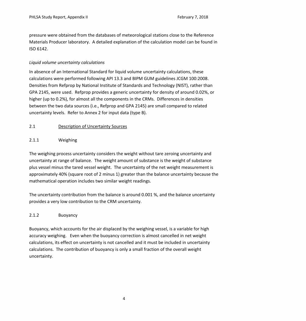
MOLECULAR WEIGHT
BENZENE BALANCE INDICATION
MANUAL KNOBADJUSTMENT
MOLECULAR WEIGHT UNCERTAINTY
N-NONANE BALANCE INDICATION
N-NONANE MOLECULARWEIGHT
STANDARD CALCULATEDRESPONSE
BENZENE BALANCE INDICATION
SAMPLE BALANCE INDICATION
CRYOSCOPE PRECISION
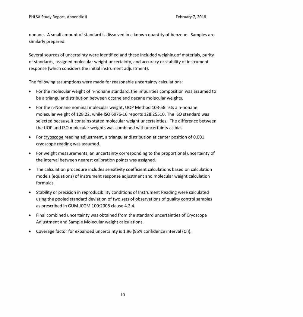
Figure 2-2. Sources of uncertainty for molecular weight measurements
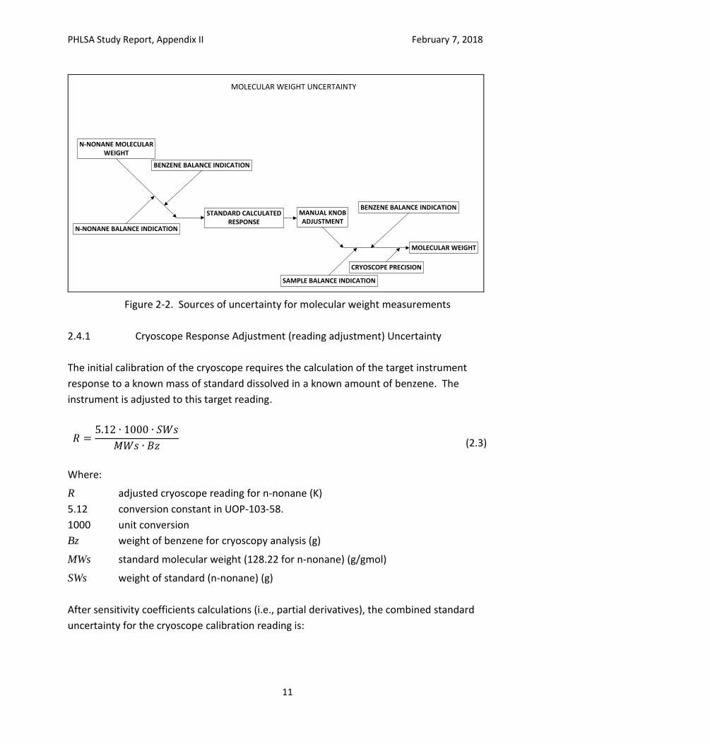
2.4.1 Cryoscope Response Adjustment (reading adjustment) Uncertainty
The initial calibration of the cryoscope requires the calculation of the target instrument
response to a known mass of standard dissolved in a known amount of benzene. The
instrument is adjusted to this target reading.
𝑅 =5.12 ∙ 1000 ∙ 𝑆𝑊𝑠
𝑀𝑊𝑠 ∙ 𝐵𝑧 (2.3)
Where:
R adjusted cryoscope reading for n-nonane (K)
5.12 conversion constant in UOP-103-58.
1000 unit conversion
Bz weight of benzene for cryoscopy analysis (g)
MWs standard molecular weight (128.22 for n-nonane) (g/gmol)
SWs weight of standard (n-nonane) (g)
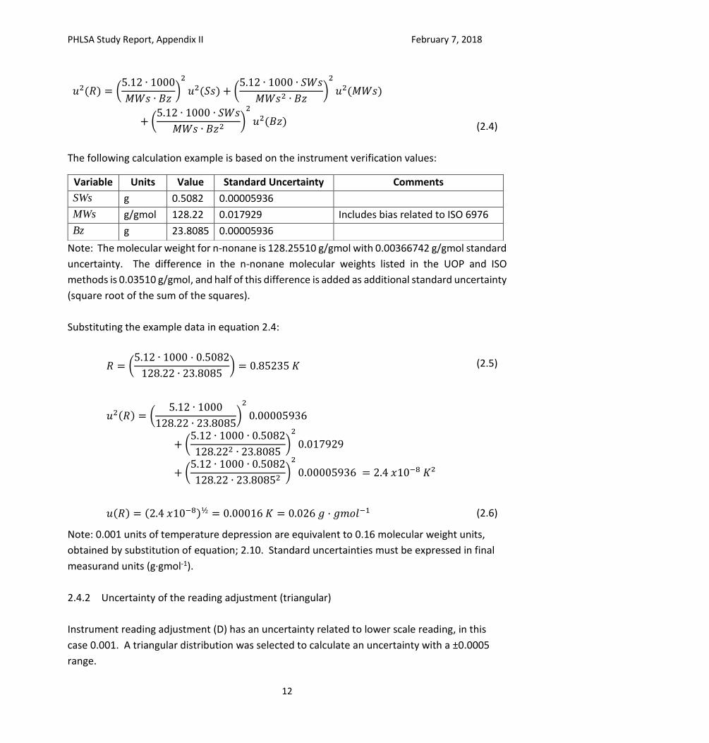
After sensitivity coefficients calculations (i.e., partial derivatives), the combined standard
uncertainty for the cryoscope calibration reading is:
PHLSA Study Report, Appendix II February 7, 2018
12
𝑢2(𝑅) = (5.12 ∙ 1000
𝑀𝑊𝑠 ∙ 𝐵𝑧)2
𝑢2(𝑆𝑠) + (5.12 ∙ 1000 ∙ 𝑆𝑊𝑠
𝑀𝑊𝑠2 ∙ 𝐵𝑧)2
𝑢2(𝑀𝑊𝑠)
+ (5.12 ∙ 1000 ∙ 𝑆𝑊𝑠
𝑀𝑊𝑠 ∙ 𝐵𝑧2)2
𝑢2(𝐵𝑧) (2.4)
The following calculation example is based on the instrument verification values:
Note: The molecular weight for n-nonane is 128.25510 g/gmol with 0.00366742 g/gmol standard
uncertainty. The difference in the n-nonane molecular weights listed in the UOP and ISO
methods is 0.03510 g/gmol, and half of this difference is added as additional standard uncertainty
(square root of the sum of the squares).
Substituting the example data in equation 2.4:
𝑅 = (5.12 ∙ 1000 · 0.5082
128.22 ∙ 23.8085) = 0.85235 𝐾 (2.5)
𝑢2(𝑅) = (5.12 ∙ 1000
128.22 ∙ 23.8085)2
0.00005936
+ (5.12 ∙ 1000 ∙ 0.5082
128.222 ∙ 23.8085)
2
0.017929
+ (5.12 ∙ 1000 ∙ 0.5082
128.22 ∙ 23.80852)
2
0.00005936 = 2.4 𝑥10−8 𝐾²
𝑢(𝑅) = (2.4 𝑥10−8)½ = 0.00016 𝐾 = 0.026 𝑔 · 𝑔𝑚𝑜𝑙−1 (2.6)
Note: 0.001 units of temperature depression are equivalent to 0.16 molecular weight units,
obtained by substitution of equation; 2.10. Standard uncertainties must be expressed in final
measurand units (g·gmol-1).
2.4.2 Uncertainty of the reading adjustment (triangular)
Instrument reading adjustment (D) has an uncertainty related to lower scale reading, in this
case 0.001. A triangular distribution was selected to calculate an uncertainty with a ±0.0005
range.
Variable Units Value Standard Uncertainty Comments
SWs g 0.5082 0.00005936
MWs g/gmol 128.22 0.017929 Includes bias related to ISO 6976
Bz g 23.8085 0.00005936
PHLSA Study Report, Appendix II February 7, 2018
13
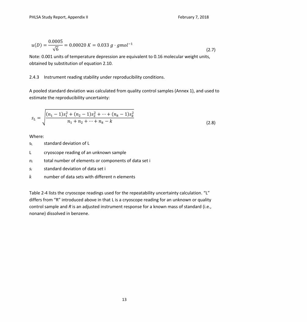
𝑢(𝐷) =0.0005
√6= 0.00020 𝐾 = 0.033 𝑔 · 𝑔𝑚𝑜𝑙−1
(2.7)
Note: 0.001 units of temperature depression are equivalent to 0.16 molecular weight units,
obtained by substitution of equation 2.10.
2.4.3 Instrument reading stability under reproducibility conditions.
A pooled standard deviation was calculated from quality control samples (Annex 1), and used to
estimate the reproducibility uncertainty:
𝑠𝐿 = √(𝑛1 − 1)𝑠1
2 + (𝑛2 − 1)𝑠22 + ⋯+ (𝑛𝑘 − 1)𝑠𝑘
2
𝑛1 + 𝑛2 + ⋯+ 𝑛𝑘 − 𝑘
(2.8)
Where:
sL standard deviation of L
L cryoscope reading of an unknown sample
ni total number of elements or components of data set i
si standard deviation of data set i
k number of data sets with different n elements
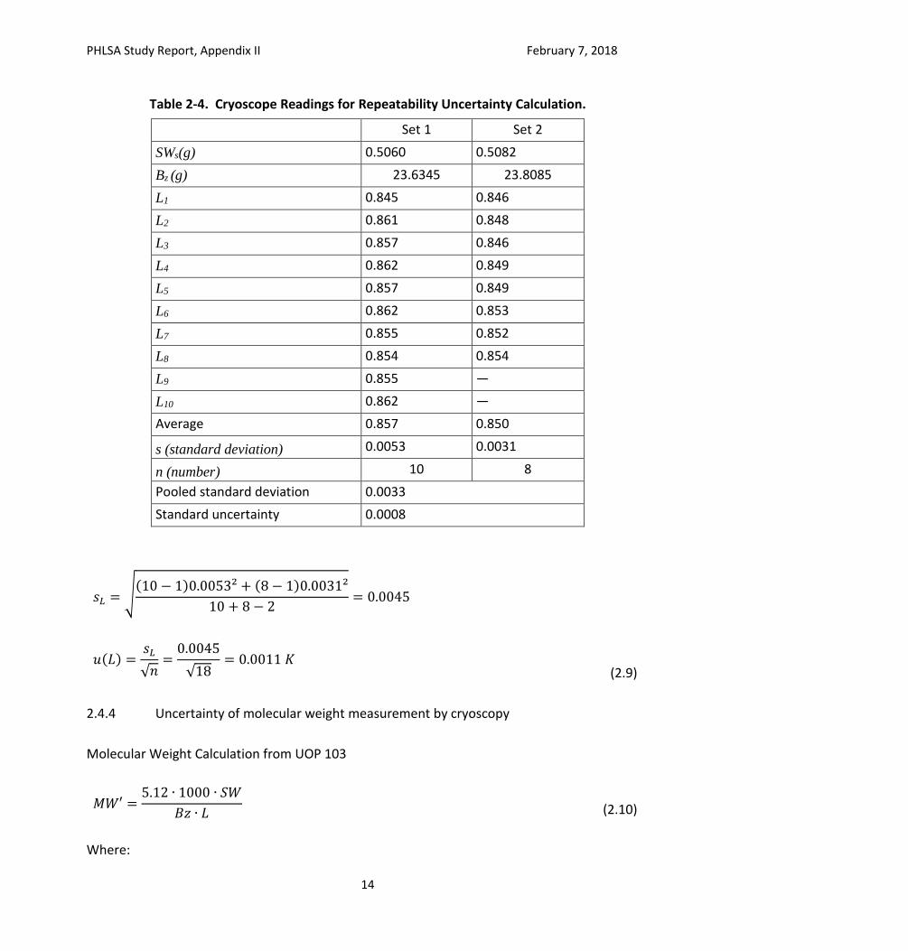
Table 2-4 lists the cryoscope readings used for the repeatability uncertainty calculation. “L”
differs from “R” introduced above in that L is a cryoscope reading for an unknown or quality
control sample and R is an adjusted instrument response for a known mass of standard (i.e.,
nonane) dissolved in benzene.
PHLSA Study Report, Appendix II February 7, 2018
14
Table 2-4. Cryoscope Readings for Repeatability Uncertainty Calculation.
Set 1 Set 2
SWs(g) 0.5060 0.5082
Bz (g) 23.6345 23.8085
L1 0.845 0.846
L2 0.861 0.848
L3 0.857 0.846
L4 0.862 0.849
L5 0.857 0.849
L6 0.862 0.853
L7 0.855 0.852
L8 0.854 0.854
L9 0.855 —
L10 0.862 —
Average 0.857 0.850
s (standard deviation) 0.0053 0.0031
n (number) 10 8
Pooled standard deviation 0.0033
Standard uncertainty 0.0008
𝑠𝐿 = √(10 − 1)0.0053² + (8 − 1)0.0031²
10 + 8 − 2= 0.0045
𝑢(𝐿) =𝑠𝐿
√𝑛=
0.0045
√18= 0.0011 𝐾
(2.9)
2.4.4 Uncertainty of molecular weight measurement by cryoscopy
Molecular Weight Calculation from UOP 103
𝑀𝑊′ =5.12 ∙ 1000 ∙ 𝑆𝑊
𝐵𝑧 ∙ 𝐿 (2.10)
Where:
PHLSA Study Report, Appendix II February 7, 2018
15
MW’ Calculated Molecular Weight (g/gmol)
SW Sample weight for Cryoscopy Analysis (g)
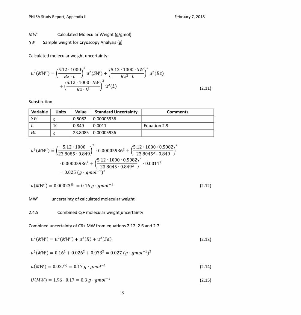
Calculated molecular weight uncertainty:
𝑢2(𝑀𝑊′) = (5.12 ∙ 1000
𝐵𝑧 ∙ 𝐿)2
𝑢2(𝑆𝑊) + (5.12 ∙ 1000 ∙ 𝑆𝑊
𝐵𝑧2 ∙ 𝐿)2
𝑢2(𝐵𝑧)
+ (5.12 ∙ 1000 ∙ 𝑆𝑊
𝐵𝑧 ∙ 𝐿2)2
𝑢2(𝐿) (2.11)
Substitution:
𝑢2(𝑀𝑊′) = (5.12 ∙ 1000
23.8085 ∙ 0.849)2
· 0.000059362 + (5.12 ∙ 1000 ∙ 0.5082
23.80452 ∙ 0.849)2
· 0.000059362 + (5.12 ∙ 1000 ∙ 0.5082
23.8045 ∙ 0.8492)2
· 0.00112
= 0.025 (𝑔 · 𝑔𝑚𝑜𝑙−1)²
𝑢(𝑀𝑊′) = 0.00023½ = 0.16 𝑔 · 𝑔𝑚𝑜𝑙−1 (2.12)
MW’ uncertainty of calculated molecular weight
2.4.5 Combined C6+ molecular weight uncertainty
Combined uncertainty of C6+ MW from equations 2.12, 2.6 and 2.7
𝑢2(𝑀𝑊) = 𝑢2(𝑀𝑊′) + 𝑢2(𝑅) + 𝑢2(𝑆𝑑) (2.13)
𝑢2(𝑀𝑊) = 0.16² + 0.026² + 0.033² = 0.027 (𝑔 · 𝑔𝑚𝑜𝑙−1)²
𝑢(𝑀𝑊) = 0.027½ = 0.17 𝑔 · 𝑔𝑚𝑜𝑙−1 (2.14)
𝑈(𝑀𝑊) = 1.96 · 0.17 = 0.3 𝑔 · 𝑔𝑚𝑜𝑙−1 (2.15)
Variable Units Value Standard Uncertainty Comments
SW g 0.5082 0.00005936
L °K 0.849 0.0011 Equation 2.9
Bz g 23.8085 0.00005936
PHLSA Study Report, Appendix II February 7, 2018
16
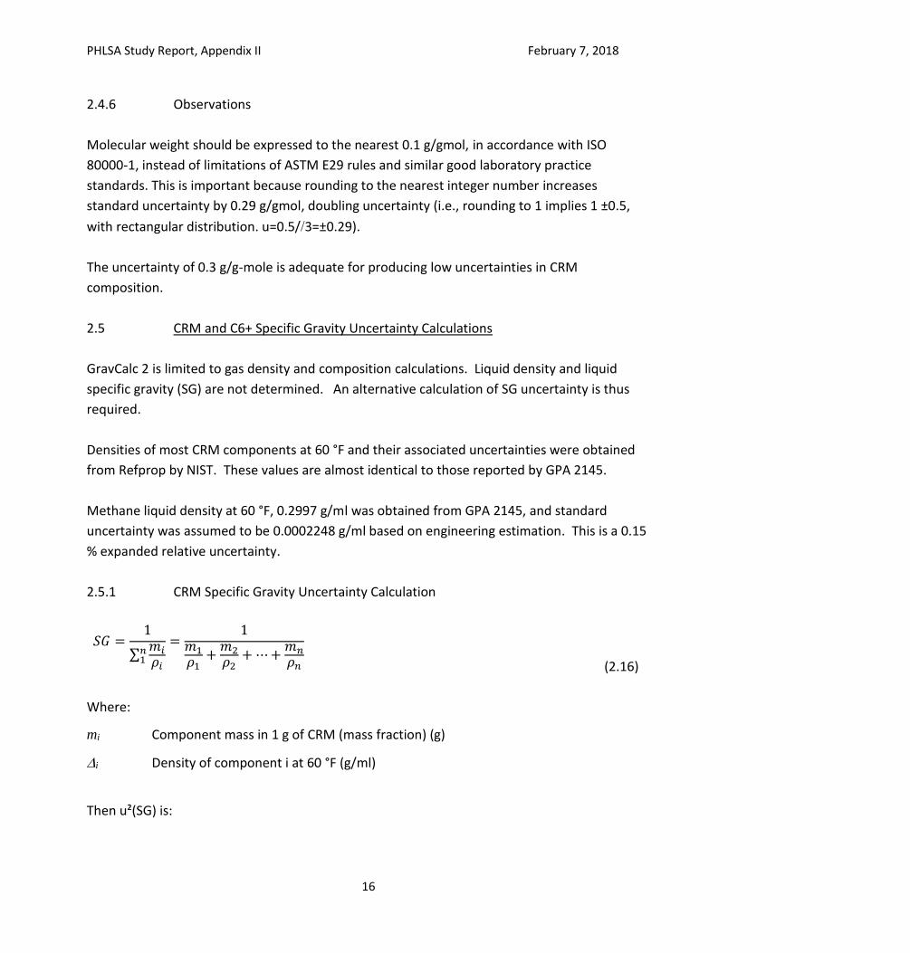
2.4.6 Observations
Molecular weight should be expressed to the nearest 0.1 g/gmol, in accordance with ISO
80000-1, instead of limitations of ASTM E29 rules and similar good laboratory practice
standards. This is important because rounding to the nearest integer number increases
standard uncertainty by 0.29 g/gmol, doubling uncertainty (i.e., rounding to 1 implies 1 ±0.5,
with rectangular distribution. u=0.5/3=±0.29).
The uncertainty of 0.3 g/g-mole is adequate for producing low uncertainties in CRM
composition.
2.5 CRM and C6+ Specific Gravity Uncertainty Calculations
GravCalc 2 is limited to gas density and composition calculations. Liquid density and liquid
specific gravity (SG) are not determined. An alternative calculation of SG uncertainty is thus
required.
Densities of most CRM components at 60 °F and their associated uncertainties were obtained
from Refprop by NIST. These values are almost identical to those reported by GPA 2145.
Methane liquid density at 60 °F, 0.2997 g/ml was obtained from GPA 2145, and standard
uncertainty was assumed to be 0.0002248 g/ml based on engineering estimation. This is a 0.15
% expanded relative uncertainty.
2.5.1 CRM Specific Gravity Uncertainty Calculation
𝑆𝐺 =1
∑𝑚𝑖
𝜌𝑖
𝑛1
=1
𝑚1
𝜌1+
𝑚2
𝜌2+ ⋯+
𝑚𝑛
𝜌𝑛
(2.16)
Where:
mi Component mass in 1 g of CRM (mass fraction) (g)
i Density of component i at 60 °F (g/ml)
Then u²(SG) is:
PHLSA Study Report, Appendix II February 7, 2018
17
𝑢2(𝑆𝐺) = ∑[((𝑚𝑖
𝜌𝑖)2
+ 1)(1
𝜌𝑖 (∑𝑚𝑖
𝜌𝑖
𝑛1 )
2)]
𝑛
𝑖=1
(2.17)
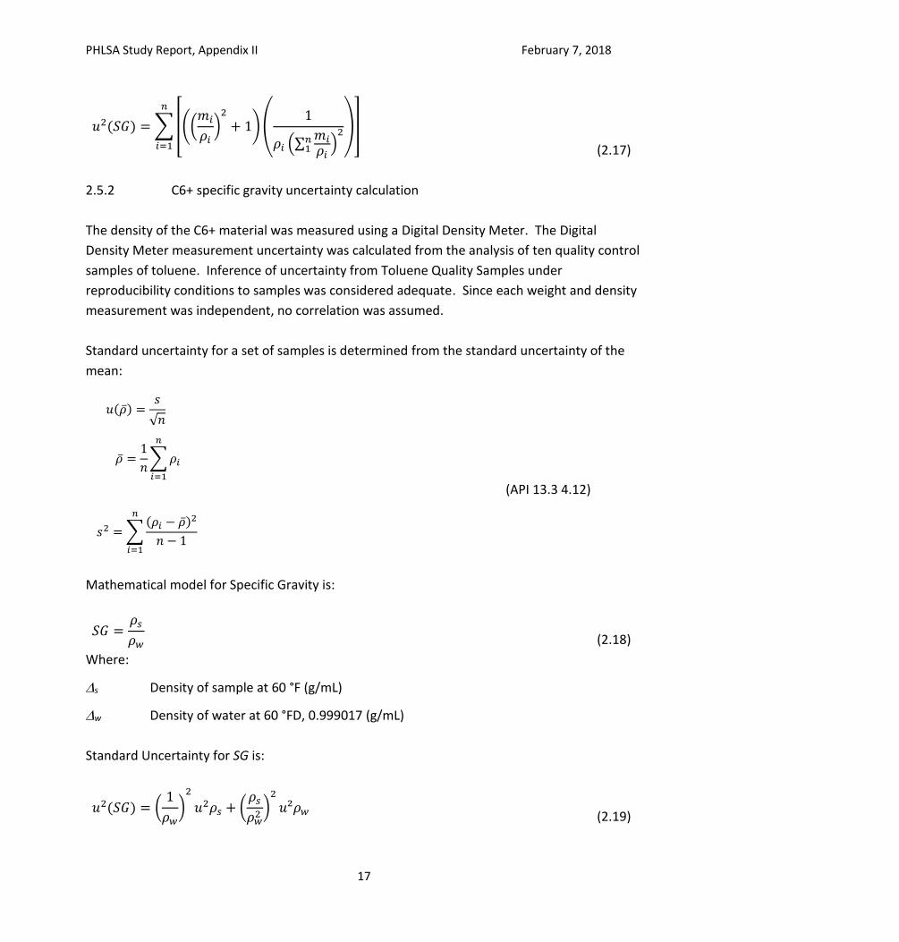
2.5.2 C6+ specific gravity uncertainty calculation
The density of the C6+ material was measured using a Digital Density Meter. The Digital
Density Meter measurement uncertainty was calculated from the analysis of ten quality control
samples of toluene. Inference of uncertainty from Toluene Quality Samples under
reproducibility conditions to samples was considered adequate. Since each weight and density
measurement was independent, no correlation was assumed.
Standard uncertainty for a set of samples is determined from the standard uncertainty of the
mean:
(API 13.3 4.12)
Mathematical model for Specific Gravity is:
𝑆𝐺 =𝜌𝑠
𝜌𝑤
(2.18)
Where:
s Density of sample at 60 °F (g/mL)
w Density of water at 60 °FD, 0.999017 (g/mL)
Standard Uncertainty for SG is:
𝑢2(𝑆𝐺) = (1
𝜌𝑤)
2
𝑢2𝜌𝑠 + (𝜌𝑠
𝜌𝑤2)
2
𝑢²𝜌𝑤 (2.19)
𝑠2 = ∑(𝜌𝑖 − �̅�)2
𝑛 − 1
𝑛
𝑖=1
𝑢(�̅�) =𝑠
√𝑛
�̅� =1
𝑛∑𝜌𝑖
𝑛
𝑖=1
PHLSA Study Report, Appendix II February 7, 2018
18
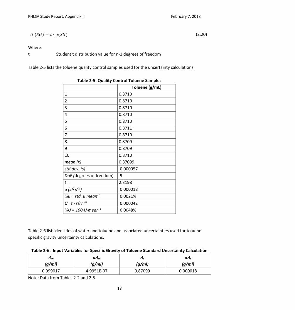
𝑈 (𝑆𝐺) = 𝑡 ∙ 𝑢(𝑆𝐺) (2.20)
Where:
t Student t distribution value for n-1 degrees of freedom
Table 2-5 lists the toluene quality control samples used for the uncertainty calculations.
Table 2-5. Quality Control Toluene Samples
Toluene (g/mL)
1 0.8710
2 0.8710
3 0.8710
4 0.8710
5 0.8710
6 0.8711
7 0.8710
8 0.8709
9 0.8709
10 0.8710
mean (x) 0.87099
std.dev. (s) 0.000057
DoF (degrees of freedom) 9
t= 2.3198
u (s n-½) 0.000018
%u = std. u·mean-1 0.0021%
U= t · s n-½ 0.000042
%U = 100·U·mean-1 0.0048%
Table 2-6 lists densities of water and toluene and associated uncertainties used for toluene
specific gravity uncertainty calculations.
Table 2-6. Input Variables for Specific Gravity of Toluene Standard Uncertainty Calculation
w
(g/ml)
uw
(g/ml)
s
(g/ml)
us
(g/ml)
0.999017 4.9951E-07 0.87099 0.000018
Note: Data from Tables 2-2 and 2-5
PHLSA Study Report, Appendix II February 7, 2018
19
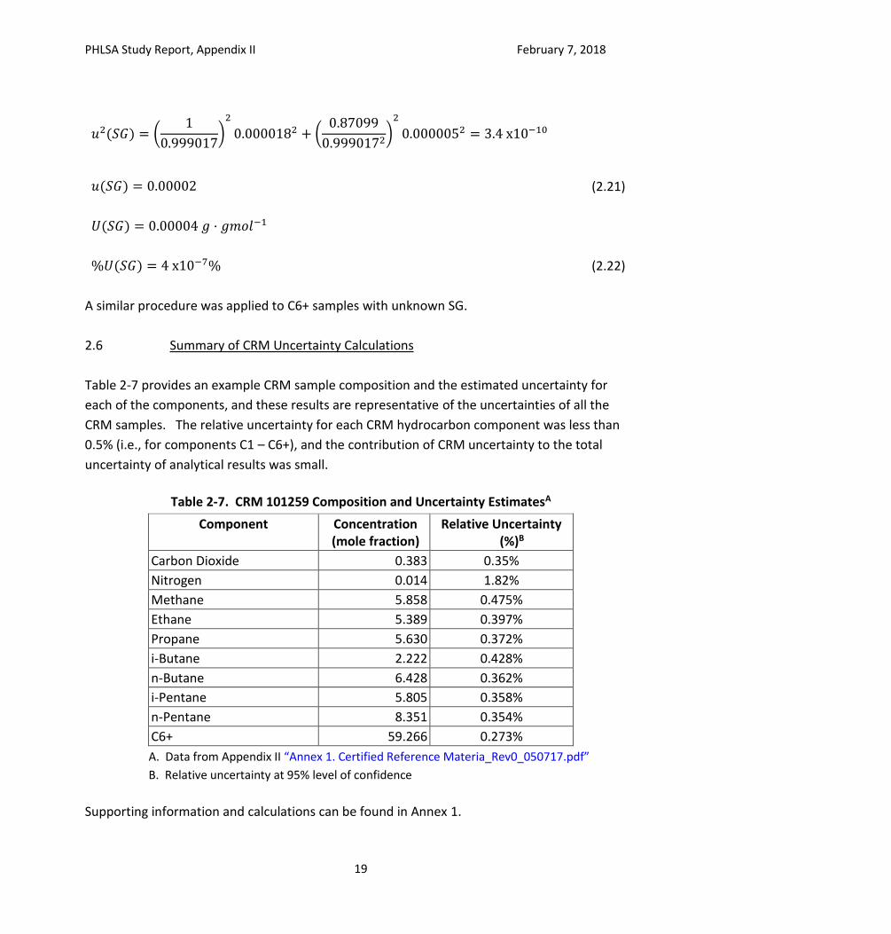
𝑢2(𝑆𝐺) = (1
0.999017)
2
0.0000182 + (0.87099
0.9990172)
2
0.0000052 = 3.4 x10⁻¹⁰
𝑢(𝑆𝐺) = 0.00002 (2.21)
𝑈(𝑆𝐺) = 0.00004 𝑔 · 𝑔𝑚𝑜𝑙−1
%𝑈(𝑆𝐺) = 4 x10⁻⁷% (2.22)
A similar procedure was applied to C6+ samples with unknown SG.
2.6 Summary of CRM Uncertainty Calculations
Table 2-7 provides an example CRM sample composition and the estimated uncertainty for
each of the components, and these results are representative of the uncertainties of all the
CRM samples. The relative uncertainty for each CRM hydrocarbon component was less than
0.5% (i.e., for components C1 – C6+), and the contribution of CRM uncertainty to the total
uncertainty of analytical results was small.
Table 2-7. CRM 101259 Composition and Uncertainty EstimatesA
Component Concentration (mole fraction)
Relative Uncertainty (%)B
Carbon Dioxide 0.383 0.35%
Nitrogen 0.014 1.82%
Methane 5.858 0.475%
Ethane 5.389 0.397%
Propane 5.630 0.372%
i-Butane 2.222 0.428%
n-Butane 6.428 0.362%
i-Pentane 5.805 0.358%
n-Pentane 8.351 0.354%
C6+ 59.266 0.273%
A. Data from Appendix II “Annex 1. Certified Reference Materia_Rev0_050717.pdf”
B. Relative uncertainty at 95% level of confidence
Supporting information and calculations can be found in Annex 1.
PHLSA Study Report, Appendix II February 7, 2018
20
3. Multi-laboratory Study
Supporting data and calculations for the information presented in this section can be found in
Annex 2.
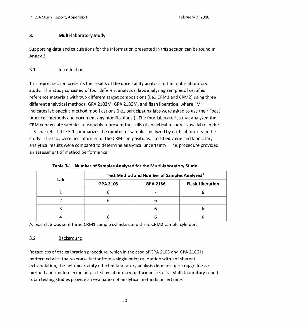
3.1 Introduction
This report section presents the results of the uncertainty analysis of the multi-laboratory
study. This study consisted of four different analytical labs analyzing samples of certified
reference materials with two different target compositions (I.e., CRM1 and CRM2) using three
different analytical methods: GPA 2103M, GPA 2186M, and flash liberation, where “M”
indicates lab-specific method modifications (i.e., participating labs were asked to use their “best
practice” methods and document any modifications.). The four laboratories that analyzed the
CRM condensate samples reasonably represent the skills of analytical resources available in the
U.S. market. Table 3-1 summarizes the number of samples analyzed by each laboratory in the
study. The labs were not informed of the CRM compositions. Certified value and laboratory
analytical results were compared to determine analytical uncertainty. This procedure provided
an assessment of method performance.
Table 3-1. Number of Samples Analyzed for the Multi-laboratory Study
Lab Test Method and Number of Samples AnalyzedA
GPA 2103 GPA 2186 Flash Liberation
1 6 - 6
2 6 6 -
3 - 6 6
4 6 6 6
A. Each lab was sent three CRM1 sample cylinders and three CRM2 sample cylinders.
3.2 Background
Regardless of the calibration procedure, which in the case of GPA 2103 and GPA 2186 is
performed with the response factor from a single point calibration with an inherent
extrapolation, the net uncertainty effect of laboratory analysis depends upon ruggedness of
method and random errors impacted by laboratory performance skills. Multi-laboratory round-
robin testing studies provide an evaluation of analytical methods uncertainty.
PHLSA Study Report, Appendix II February 7, 2018
21
Available International standards for method precision assessment based on an Inter-
Laboratory Study are ISO 5725 series and ASTM D6300. For an Inter-Laboratory Study, 30 or
more laboratories are recommended (ASTM E691, Clause 9.1.1), but when this is not practical,
8 laboratories could be enough. Under no circumstances should the final statement of
precision of a test method be based from fewer than 6 laboratories (ibidem Clause 9.1.2). In
any case, it is necessary to obtain at least 30 degrees of freedom (ASTM D6300, Clause 6.4.2)
for determinations of both repeatability and reproducibility. For repeatability, this means
obtaining a total of at least 30 pairs of results in the program.
Because the number of laboratories and sample pairs for the multi-lab study are not compliant
with these recommendations, the referenced methods limit any statistical deductions to a
general conclusions statement. Thus, uncertainty calculations were performed similar to the
practice of individual laboratories analysis of reference materials as stated in ISO 6974 series
(for natural gas analysis). These include calculating uncertainty using errors in a linear
regression analysis, which is appropriate for single point calibration methods.
3.3 Approach
The data set was first evaluated for outliers, and then a linear regression model was used to
analyze the multi-laboratory results and conduct an uncertainty analysis to evaluate:
• Relative performance of the three analytical methods by estimating each method’s
uncertainty for each CRM compound; and
• Relative performance of the four analytical labs.
3.3.1 Outliers
The GPA 2103 CRM analysis data reported by Laboratory 1 appeared to be very different from
the reference values and the results of the other laboratories. To determine if rejection of
outliers was statistically supported, outlier identification procedures were conducted in
accordance with two techniques, Mandel's h statistic and API MPMS 13.1.8.1.2 through Dixon's
Q test. Complete statistical treatment used for outlier identification was performed in
accordance with the ISO 5725-2 method.
Dixon´s Q test results for n-hexane results are presented in Table 3-2. The average of three
results of the levels was used to preclude masking effects from multiple outliers. The Q test
critical value for three results is 0.941 for 90% and 0.970 for 95%. For this data, only the 4th
PHLSA Study Report, Appendix II February 7, 2018
22
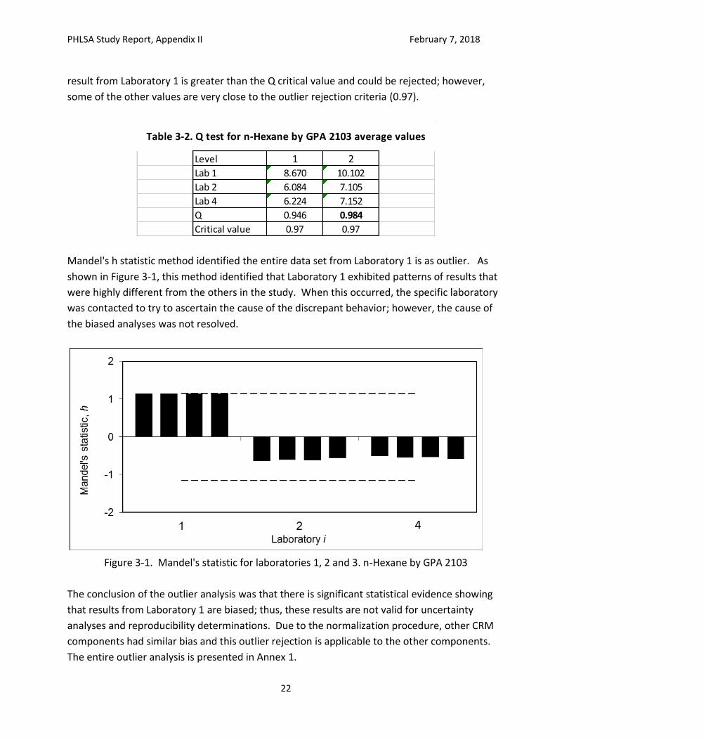
result from Laboratory 1 is greater than the Q critical value and could be rejected; however,
some of the other values are very close to the outlier rejection criteria (0.97).
Mandel's h statistic method identified the entire data set from Laboratory 1 is as outlier. As
shown in Figure 3-1, this method identified that Laboratory 1 exhibited patterns of results that
were highly different from the others in the study. When this occurred, the specific laboratory
was contacted to try to ascertain the cause of the discrepant behavior; however, the cause of
the biased analyses was not resolved.
Figure 3-1. Mandel's statistic for laboratories 1, 2 and 3. n-Hexane by GPA 2103
The conclusion of the outlier analysis was that there is significant statistical evidence showing
that results from Laboratory 1 are biased; thus, these results are not valid for uncertainty
analyses and reproducibility determinations. Due to the normalization procedure, other CRM
components had similar bias and this outlier rejection is applicable to the other components.
The entire outlier analysis is presented in Annex 1.
Level 1 2Lab 1 8.670 10.102
Lab 2 6.084 7.105
Lab 4 6.224 7.152
Q 0.946 0.984
Critical value 0.97 0.97
Table 3-2. Q test for n-Hexane by GPA 2103 average values
PHLSA Study Report, Appendix II February 7, 2018
23
Rejection of Lab 1 results reduced the average bias, and the remaining data were determined
to be suitable for laboratory bias performance assessment.
3.3.2 Overview of the uncertainty calculations
Uncertainty calculations were performed following methodology from API MPMS 13.3
"Measurement Uncertainty". The procedure compared the CRM reference composition and
the analytical results from each lab to estimate the associated analytical uncertainty. For each
pressurized condensate component, a first order regression model was developed using CRM
values as independent variables and associated lab results as dependent variables, and the
uncertainties of analytical results were estimated from the uncertainties in the slopes and y-
intercepts of the linear regression models. This approach is in accordance with NIST
Engineering Statistic Handbook, 2.3.6.7.3, and was used because much relevant information
regarding calibration and traceability was not available from all participant laboratories, and a
black box model can overcome this issue. Additionally, a Monte Carlo simulation was
performed for procedure validation and provided similar results.
Section 3.4 presents the general equations for uncertainty calculations. The n-hexane
calculation is presented in section 3.5 as an example of the general procedure for uncertainty
calculations. The same uncertainty analysis model and procedure, based on experimental data,
was applied to all components of analytical methods.
Finally, overall results of components and/or methods are compared using graphical
representation and associated uncertainties are identified. These evaluations may be used to
select a preferred method for a given application.
3.4 General Equations for Uncertainty Calculations
3.4.1 Measurement model
The measurement model was developed considering the reported data as the dependent
variable and the CRM value as the independent variable, and a first order linear regression was
found appropriate to represent behavior of analytical methods. Evaluation with a second order
function did not show significant improvement.
Analytical data assessment was based on the following function:
PHLSA Study Report, Appendix II February 7, 2018
24
𝑅𝑣 = 𝑎 𝐶𝑣 + 𝑏 (3.1)
Where:
a Slope constant of first order regression (dimensionless)
b Ordinate to origin or intercept constant of first order regression (dimensionless)
Cv Reference (CRM) value of component for multi-laboratory study, independent
variable in linear regression
Rv Reported analytical value in multi-laboratory study, dependent variable in linear
regression
If the analytical results equaled the CRM values, then the results of the linear regression would
be “a” = 1.0 and “b” = zero.
Sensitivity Coefficients determination:
Sensitivity coefficients quantify the effect of the uncertainty of a component on the total
uncertainty estimate. The sensitivity coefficient of x with respect to y is defined by the first
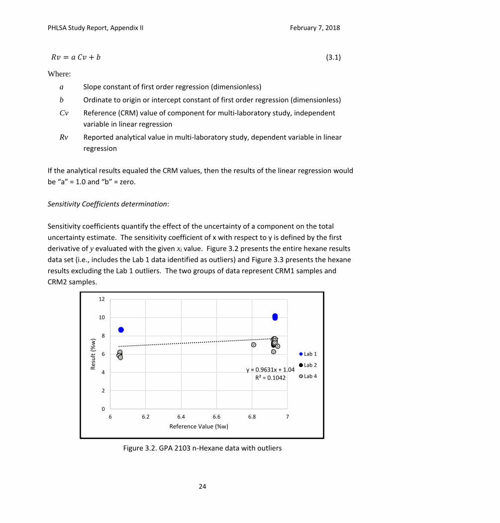
derivative of y evaluated with the given xi value. Figure 3.2 presents the entire hexane results
data set (i.e., includes the Lab 1 data identified as outliers) and Figure 3.3 presents the hexane
results excluding the Lab 1 outliers. The two groups of data represent CRM1 samples and
CRM2 samples.
Figure 3.2. GPA 2103 n-Hexane data with outliers
y = 0.9631x + 1.04R² = 0.1042
0
2
4
6
8
10
12
6 6.2 6.4 6.6 6.8 7
Res
ult
(%
w)
Reference Value (%w)
Lab 1
Lab 2
Lab 4
PHLSA Study Report, Appendix II February 7, 2018
25
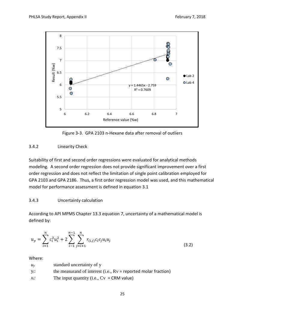
Figure 3-3. GPA 2103 n-Hexane data after removal of outliers
3.4.2 Linearity Check
Suitability of first and second order regressions were evaluated for analytical methods
modeling. A second order regression does not provide significant improvement over a first
order regression and does not reflect the limitation of single point calibration employed for
GPA 2103 and GPA 2186. Thus, a first order regression model was used, and this mathematical
model for performance assessment is defined in equation 3.1
3.4.3 Uncertainty calculation
According to API MPMS Chapter 13.3 equation 7, uncertainty of a mathematical model is
defined by:
𝑢𝑦 = ∑𝑐𝑖2𝑢𝑖
2 + 2 ∑ ∑ 𝑟(𝑖,𝑗)𝑐𝑖𝑐𝑗𝑢𝑖𝑢𝑗
𝑛
𝑗=𝑖+1
𝑛−1
𝑖−1
𝑛
𝑖=1
(3.2)
Where:
uy
yi:
standard uncertainty of y
the measurand of interest (i.e., Rv = reported molar fraction)
xi: The input quantity (i.e., Cv = CRM value)
y = 1.4465x - 2.759R² = 0.7609
5
5.5
6
6.5
7
7.5
8
6 6.2 6.4 6.6 6.8 7
Res
ult
(%
w)
Reference value (%w)
Lab 2
Lab 4
PHLSA Study Report, Appendix II February 7, 2018
26
ci:
ui
Sensitivity coefficient of the input quantity ( xi)
The standard uncertainty of input xi
r(x,j):
n:
Correlation coefficient of xi to xj
Total number of elements in the measurement model equation
Correlation is the degree of relationship between two variables. It is assumed that correlation
coefficients quantify the intensity and direction of a linear relationship between elements in
two sets of measurements, and is defined by the following equation (API MPMS Chapter 13.3
equation 6):
𝑟(𝑥𝑖,𝑗𝑖)=
∑ (𝑥𝑖 − �̅�)(𝑥𝑖 − 𝑗)̅𝑛𝑖=1
∑ (𝑥𝑖 − �̅�)2 ∑ (𝑗𝑖 − 𝑗)̅2𝑛𝑖=1
𝑛𝑖=1
(3.3)
Where:
r(xi, ji): Correlation coefficient
Based on this approach, uncertainty calculation of the first order linear regression model is
equation 3.4:
𝑢𝑦 = 𝑐𝑎2𝑢𝑎
2 + 𝑐𝑏2𝑢𝑏
2 + 2𝑟(𝑎,𝑏)𝑐𝑎𝑐𝑏𝑢𝑎𝑢𝑏 (3.4)
Where:
ca: Slope sensitivity coefficient
ua: Slope uncertainty (a regression standard error)
cb: Ordinate to the origin sensitivity coefficient
ub: Ordinate to the origin uncertainty (b regression standard error)
r(a,b): Correlation coefficient of Slope and Ordinate to the origin
The standard error of estimates of slope and intercept were used to estimate the uncertainty of
these variables (NIST Engineering Statistic Handbook, 2.3.6.7.3.).
Sensitivity coefficients are derived from the first order linear regression and correlation
element.
𝑐x = 𝜕𝑦
𝜕x (3.5)
PHLSA Study Report, Appendix II February 7, 2018
27
Where:
𝜕𝑦
𝜕x
is the partial derivative of y with respect to x
Calculations for regression, covariance and correlation matrices were performed with R Code (R
Foundation for Statistical Computing, Vienna, Austria. URL https://www.R-project.org/.)
Examples code and calculation results are included in Annex 2. Validation of uncertainty
calculations using GUM procedure was performed with GumSim. This also provides a Monte
Carlo simulation result with a confirmed value equal to the GUM procedure calculations due to
normal distribution assumptions.
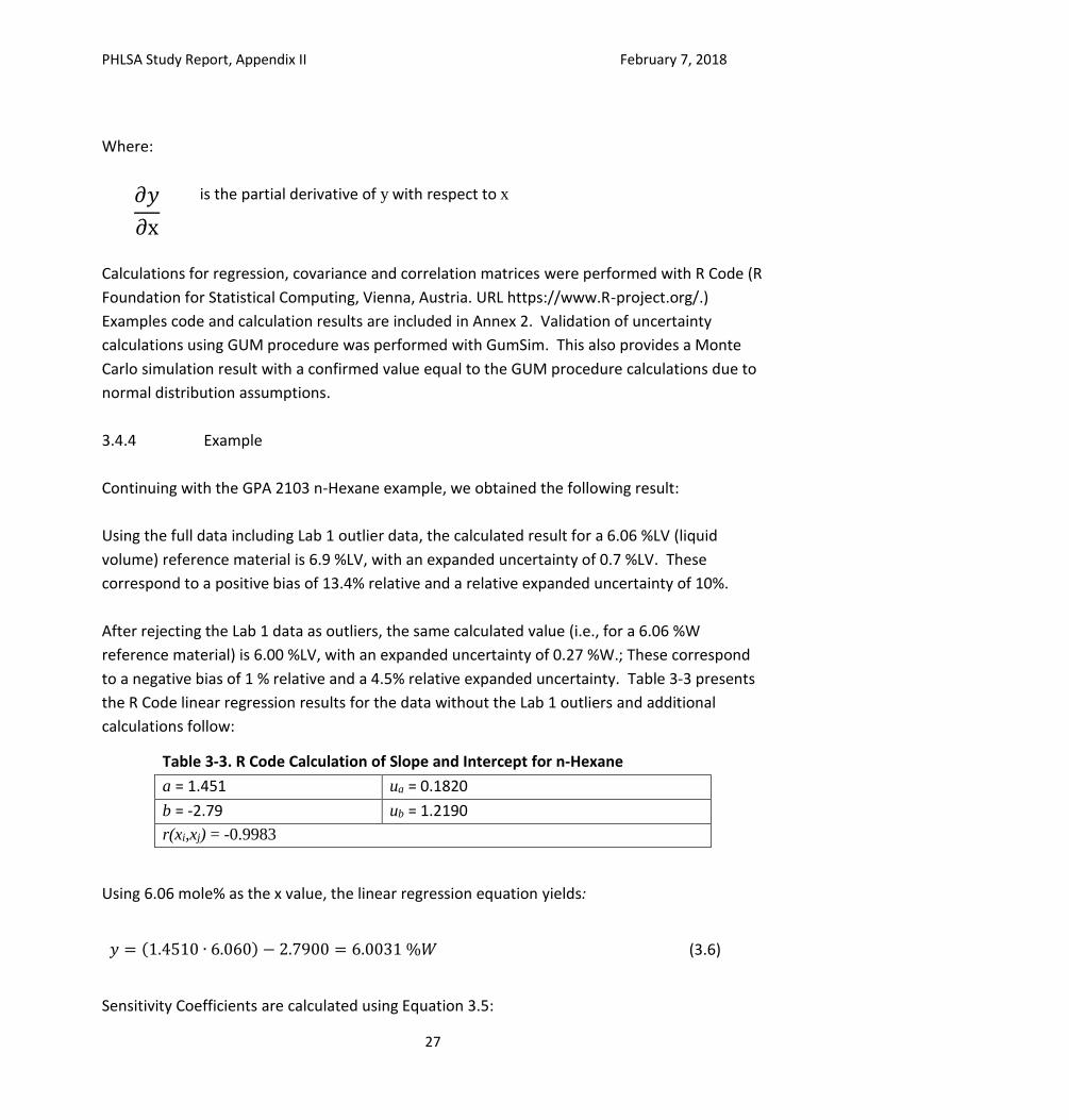
3.4.4 Example
Continuing with the GPA 2103 n-Hexane example, we obtained the following result:
Using the full data including Lab 1 outlier data, the calculated result for a 6.06 %LV (liquid
volume) reference material is 6.9 %LV, with an expanded uncertainty of 0.7 %LV. These
correspond to a positive bias of 13.4% relative and a relative expanded uncertainty of 10%.
After rejecting the Lab 1 data as outliers, the same calculated value (i.e., for a 6.06 %W
reference material) is 6.00 %LV, with an expanded uncertainty of 0.27 %W.; These correspond
to a negative bias of 1 % relative and a 4.5% relative expanded uncertainty. Table 3-3 presents
the R Code linear regression results for the data without the Lab 1 outliers and additional
calculations follow:
Table 3-3. R Code Calculation of Slope and Intercept for n-Hexane
a = 1.451 ua = 0.1820
b = -2.79 ub = 1.2190
r(xi,xj) = -0.9983
Using 6.06 mole% as the x value, the linear regression equation yields:
𝑦 = (1.4510 ∙ 6.060) − 2.7900 = 6.0031 %𝑊 (3.6)
Sensitivity Coefficients are calculated using Equation 3.5:
PHLSA Study Report, Appendix II February 7, 2018
28
Original model: 𝑦 = 𝑎𝑥 + 𝑏
𝑐𝑎 =𝑑𝑦
𝑑𝑎=
𝜕(𝑎𝑥𝑖 + 𝑏)
𝜕𝑎= 𝑥𝑖 (3.7)
𝑐𝑏 =𝑑𝑦
𝑑𝑏=
𝜕(𝑎𝑥𝑖 + 𝑏)
𝜕𝑏= 1 (3.8)
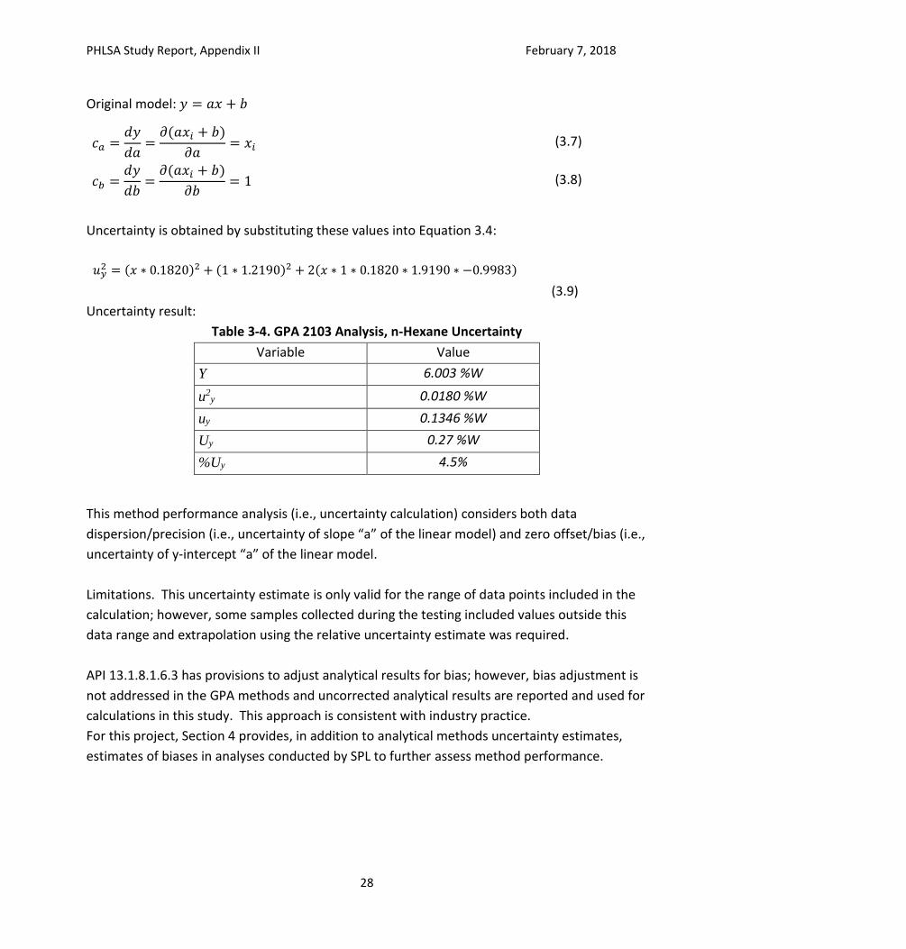
Uncertainty is obtained by substituting these values into Equation 3.4:
𝑢𝑦2 = (𝑥 ∗ 0.1820)2 + (1 ∗ 1.2190)2 + 2(𝑥 ∗ 1 ∗ 0.1820 ∗ 1.9190 ∗ −0.9983)
(3.9)
Uncertainty result:
Table 3-4. GPA 2103 Analysis, n-Hexane Uncertainty
Variable Value
Y 6.003 %W
u2y 0.0180 %W
uy 0.1346 %W
Uy 0.27 %W
%Uy 4.5%
This method performance analysis (i.e., uncertainty calculation) considers both data
dispersion/precision (i.e., uncertainty of slope “a” of the linear model) and zero offset/bias (i.e.,
uncertainty of y-intercept “a” of the linear model.
Limitations. This uncertainty estimate is only valid for the range of data points included in the
calculation; however, some samples collected during the testing included values outside this
data range and extrapolation using the relative uncertainty estimate was required.
API 13.1.8.1.6.3 has provisions to adjust analytical results for bias; however, bias adjustment is
not addressed in the GPA methods and uncorrected analytical results are reported and used for
calculations in this study. This approach is consistent with industry practice.
For this project, Section 4 provides, in addition to analytical methods uncertainty estimates,
estimates of biases in analyses conducted by SPL to further assess method performance.
PHLSA Study Report, Appendix II February 7, 2018
29
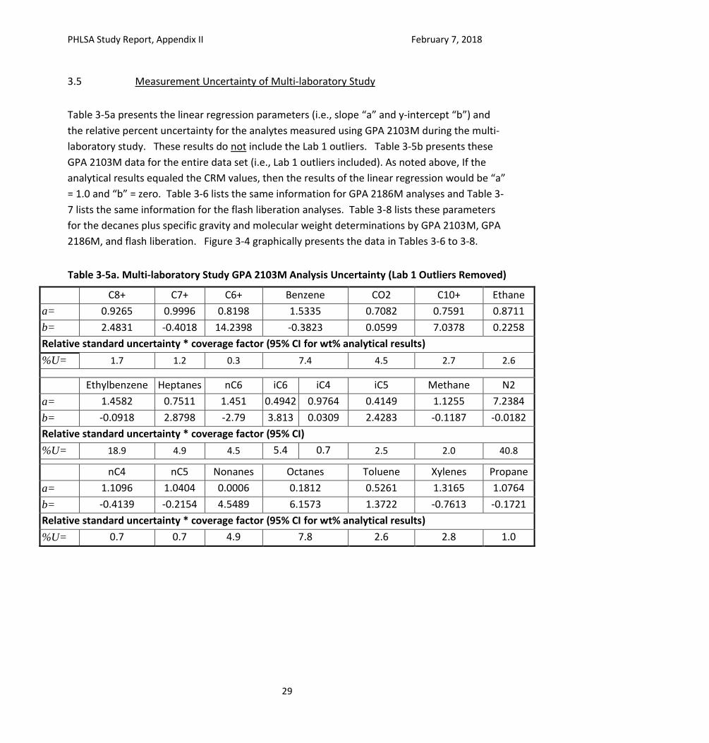
3.5 Measurement Uncertainty of Multi-laboratory Study
Table 3-5a presents the linear regression parameters (i.e., slope “a” and y-intercept “b”) and
the relative percent uncertainty for the analytes measured using GPA 2103M during the multi-
laboratory study. These results do not include the Lab 1 outliers. Table 3-5b presents these
GPA 2103M data for the entire data set (i.e., Lab 1 outliers included). As noted above, If the
analytical results equaled the CRM values, then the results of the linear regression would be “a”
= 1.0 and “b” = zero. Table 3-6 lists the same information for GPA 2186M analyses and Table 3-
7 lists the same information for the flash liberation analyses. Table 3-8 lists these parameters
for the decanes plus specific gravity and molecular weight determinations by GPA 2103M, GPA
2186M, and flash liberation. Figure 3-4 graphically presents the data in Tables 3-6 to 3-8.
Table 3-5a. Multi-laboratory Study GPA 2103M Analysis Uncertainty (Lab 1 Outliers Removed)
C8+ C7+ C6+ Benzene CO2 C10+ Ethane
a= 0.9265 0.9996 0.8198 1.5335 0.7082 0.7591 0.8711
b= 2.4831 -0.4018 14.2398 -0.3823 0.0599 7.0378 0.2258
Relative standard uncertainty * coverage factor (95% CI for wt% analytical results)
%U= 1.7 1.2 0.3 7.4 4.5 2.7 2.6 Ethylbenzene Heptanes nC6 iC6 iC4 iC5 Methane N2
a= 1.4582 0.7511 1.451 0.4942 0.9764 0.4149 1.1255 7.2384
b= -0.0918 2.8798 -2.79 3.813 0.0309 2.4283 -0.1187 -0.0182
Relative standard uncertainty * coverage factor (95% CI)
%U= 18.9 4.9 4.5 5.4 0.7 2.5 2.0 40.8
nC4 nC5 Nonanes Octanes Toluene Xylenes Propane
a= 1.1096 1.0404 0.0006 0.1812 0.5261 1.3165 1.0764
b= -0.4139 -0.2154 4.5489 6.1573 1.3722 -0.7613 -0.1721
Relative standard uncertainty * coverage factor (95% CI for wt% analytical results)
%U= 0.7 0.7 4.9 7.8 2.6 2.8 1.0
PHLSA Study Report, Appendix II February 7, 2018
30
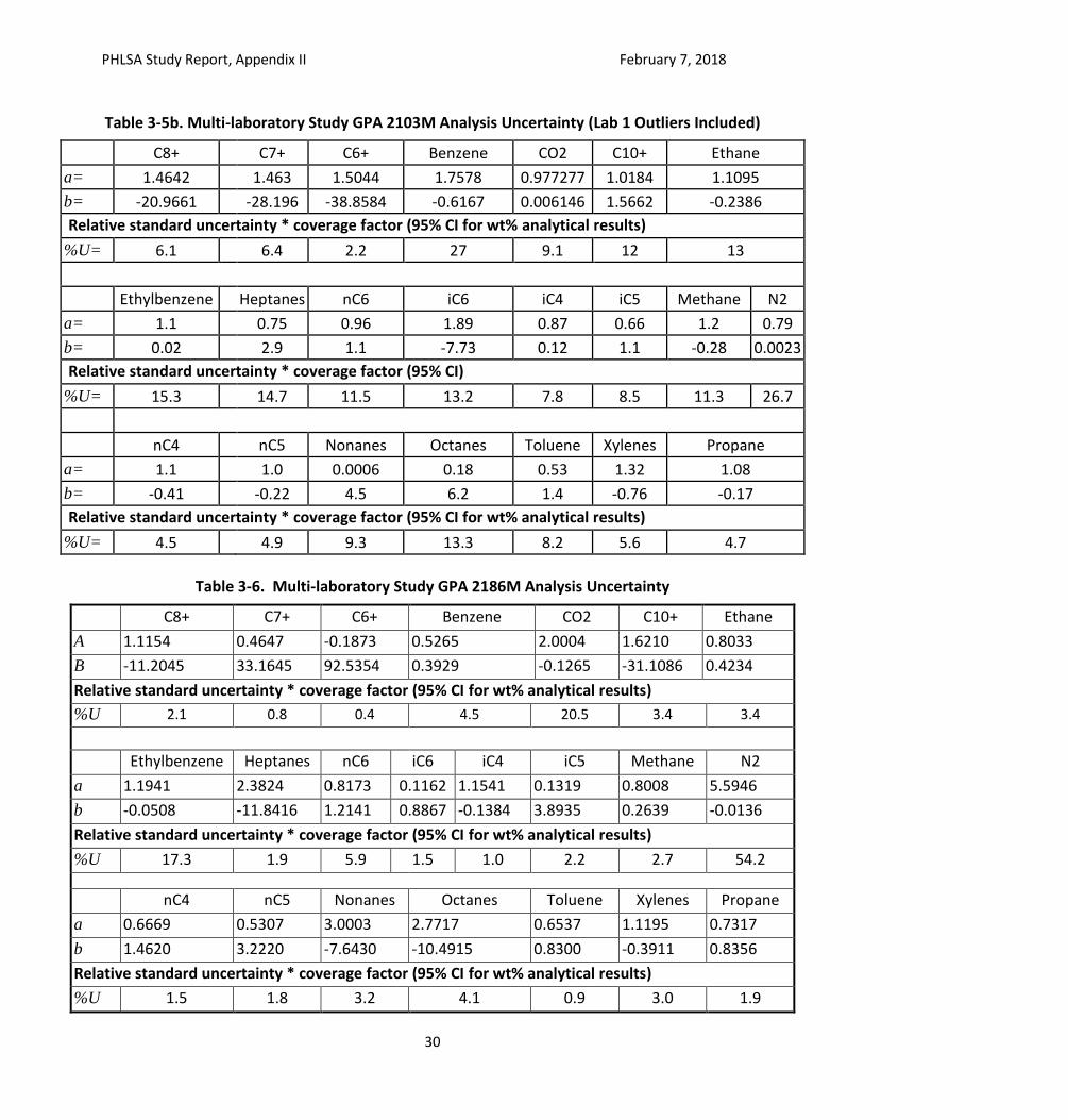
Table 3-5b. Multi-laboratory Study GPA 2103M Analysis Uncertainty (Lab 1 Outliers Included)
C8+ C7+ C6+ Benzene CO2 C10+ Ethane
a= 1.4642 1.463 1.5044 1.7578 0.977277 1.0184 1.1095
b= -20.9661 -28.196 -38.8584 -0.6167 0.006146 1.5662 -0.2386
Relative standard uncertainty * coverage factor (95% CI for wt% analytical results)
%U= 6.1 6.4 2.2 27 9.1 12 13
Ethylbenzene Heptanes nC6 iC6 iC4 iC5 Methane N2
a= 1.1 0.75 0.96 1.89 0.87 0.66 1.2 0.79
b= 0.02 2.9 1.1 -7.73 0.12 1.1 -0.28 0.0023
Relative standard uncertainty * coverage factor (95% CI)
%U= 15.3 14.7 11.5 13.2 7.8 8.5 11.3 26.7
nC4 nC5 Nonanes Octanes Toluene Xylenes Propane
a= 1.1 1.0 0.0006 0.18 0.53 1.32 1.08
b= -0.41 -0.22 4.5 6.2 1.4 -0.76 -0.17
Relative standard uncertainty * coverage factor (95% CI for wt% analytical results)
%U= 4.5 4.9 9.3 13.3 8.2 5.6 4.7
Table 3-6. Multi-laboratory Study GPA 2186M Analysis Uncertainty
C8+ C7+ C6+ Benzene CO2 C10+ Ethane
A 1.1154 0.4647 -0.1873 0.5265 2.0004 1.6210 0.8033
B -11.2045 33.1645 92.5354 0.3929 -0.1265 -31.1086 0.4234
Relative standard uncertainty * coverage factor (95% CI for wt% analytical results)
%U 2.1 0.8 0.4 4.5 20.5 3.4 3.4
Ethylbenzene Heptanes nC6 iC6 iC4 iC5 Methane N2
a 1.1941 2.3824 0.8173 0.1162 1.1541 0.1319 0.8008 5.5946
b -0.0508 -11.8416 1.2141 0.8867 -0.1384 3.8935 0.2639 -0.0136
Relative standard uncertainty * coverage factor (95% CI for wt% analytical results)
%U 17.3 1.9 5.9 1.5 1.0 2.2 2.7 54.2
nC4 nC5 Nonanes Octanes Toluene Xylenes Propane
a 0.6669 0.5307 3.0003 2.7717 0.6537 1.1195 0.7317
b 1.4620 3.2220 -7.6430 -10.4915 0.8300 -0.3911 0.8356
Relative standard uncertainty * coverage factor (95% CI for wt% analytical results)
%U 1.5 1.8 3.2 4.1 0.9 3.0 1.9
PHLSA Study Report, Appendix II February 7, 2018
31
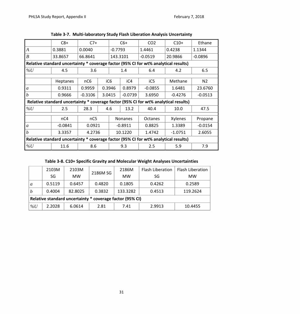
Table 3-7. Multi-laboratory Study Flash Liberation Analysis Uncertainty
C8+ C7+ C6+ CO2 C10+ Ethane
A 0.3881 0.0040 -0.7793 1.4461 0.4238 1.1344
B 33.8657 66.8641 143.3101 -0.0519 20.9866 -0.0896
Relative standard uncertainty * coverage factor (95% CI for wt% analytical results)
%U 4.5 3.6 1.4 6.4 4.2 6.5
Heptanes nC6 iC6 iC4 iC5 Methane N2
a 0.9311 0.9959 0.3946 0.8979 -0.0855 1.6481 23.6760
b 0.9666 -0.3106 3.0415 -0.0739 3.6950 -0.4276 -0.0513
Relative standard uncertainty * coverage factor (95% CI for wt% analytical results)
%U 2.5 28.3 4.6 13.2 40.4 10.0 47.5
nC4 nC5 Nonanes Octanes Xylenes Propane
a -0.0841 0.0921 -0.8911 0.8825 1.3389 -0.0154
b 3.3357 4.2736 10.1220 1.4742 -1.0751 2.6055
Relative standard uncertainty * coverage factor (95% CI for wt% analytical results)
%U 11.6 8.6 9.3 2.5 5.9 7.9
Table 3-8. C10+ Specific Gravity and Molecular Weight Analyses Uncertainties
2103M
SG
2103M
MW 2186M SG
2186M
MW
Flash Liberation
SG
Flash Liberation
MW
a 0.5119 0.6457 0.4820 0.1805 0.4262 0.2589
b 0.4004 82.8025 0.3832 133.3282 0.4513 119.2624
Relative standard uncertainty * coverage factor (95% CI)
%U 2.2028 6.0614 2.81 7.41 2.9913 10.4455
PHLSA Study Report, Appendix II February 7, 2018
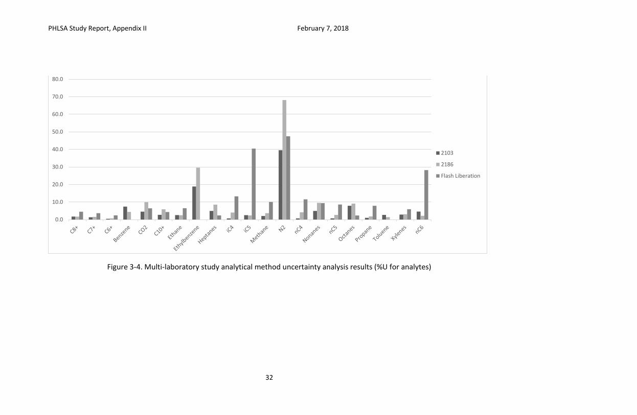
32
Figure 3-4. Multi-laboratory study analytical method uncertainty analysis results (%U for analytes)
0.0
10.0
20.0
30.0
40.0
50.0
60.0
70.0
80.0
2103
2186
Flash Liberation
PHLSA Study Report, Appendix II February 7, 2018
33
3.6 Summary of Multi-laboratory Study Findings
Primary findings of the multi-lab study include:
• One laboratory has a large bias in its GPA 2103 analytical results of CRM samples. These
results were identified as outliers and rejected. Remaining GPA 2103 results have a much
better agreement with CRM compositions. These results suggest that pre-qualification of
laboratory performance with a blind sample of known composition could be warranted.
• Relative uncertainty for nitrogen analytical results is significant at low concentrations. GPA
methods have a lower range limit of 0.01 mole percent nitrogen. For values close to or
lower than this concentration, it may be preferable to use nitrogen-free results for
subsequent calculations.
• The uncertainties of detailed analysis of pseudo-components from hexane to C10+ are
significantly greater than sum of species analytical results (e.g., U(C7) > U(C7+), U(C8) >
U(C8+)). The estimated uncertainties for hexanes, heptanes, octanes, nonanes, BTEX, and
C10+ are at least four times higher than the uncertainty estimated for total C6+ species.
The uncertainty of heptanes is on the order of three to four times greater than the
uncertainty of C7+, regardless of the method used. Well characterized lumped or total
pseudo-components provide lower uncertainties than the uncertainties of the individual
compounds.
Detailed analysis is performed over multiple peaks nested with low resolution, C6+ can be
obtained by difference with C1-C5 low uncertainty results, a more detailed analysis implies
compounds with poor resolution, this contributes to larger uncertainty. GPA 2103
analytical results generally had the lowest uncertainties, and had the lowest uncertainties
for light end compounds methane, carbon dioxide, and nitrogen.
Flash Liberation had the highest uncertainties for methane, carbon dioxide, and nitrogen.
PHLSA Study Report, Appendix II February 7, 2018
34
4. SPL Analytical Methods Evaluation
Supporting data and calculations for the information presented in this section can be found in
Annex 2.
4.1 Introduction and Approach
To assess the performance of the SPL analytical methods for pressurized condensate samples,
the SPL analytical results for CRM samples from the method performance task (Task 4 from the
Work Plan) and multi-lab study task (Task 3 from the Work Plan and addressed in Section 3)
were combined and the data analyzed to evaluate the uncertainty and bias for SPL analyses.
This resulted in 16 CRM sample analyses by SPL GPA 2186M, 16 CRM sample analyses by SPL
flash liberation, and 26 CRM sample analyses by SPL GPA 2103M. As described in Section 3,
analytical results were processed to obtain a regression between reported values and certified
values as dependent and independent variables, respectively. The uncertainty of SPL reported
results from random errors can be estimated from CRM uncertainty, linearity (linear fit errors)
and dispersion (reproducibility and repeatability). Measurement/method bias is defined as an
estimate of a systematic measurement error, and was estimated from the difference between
reported analytical values and the regression equation estimates of the analytical values based
on the associated certified (i.e., CRM) value.
According to international vocabulary of metrology (VIM) measurement bias is an estimate of a
systematic measurement error and, measurement uncertainty is a non-negative parameter
characterizing the dispersion of the quantity values being attributed to a measurand, based on
the information used.
Sometimes estimated systematic effects are not corrected for but, instead, associated
measurement uncertainty components are incorporated (API 13.1.8.1.3). As bias correction is
not addressed in GPA methods, analysis results are assumed unbiased.
On the other hand, bias cannot be assessed under routine analysis, in the best case this is
evaluated for method validation, but also, bias corrections are not applied under proper
method execution.
4.2 Summary of SPL Analytical Methods Uncertainty and Bias
Table 4-1 shows a summary of calculated uncertainties by component and method for the SPL
analytical results, and Figure 4-1 presents these results graphically. These are the uncertainties
used for subsequent uncertainty estimates, such as the uncertainties of directly measured flash
gas-to-oil ratios (FGORs) and storage tank mass balance closures. GPA 2103M generally had the
lowest uncertainties, with GPA 2186M generally having lower uncertainties than the SPL flash
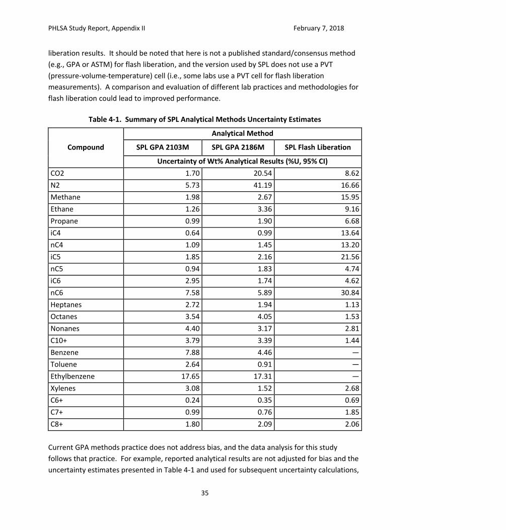
PHLSA Study Report, Appendix II February 7, 2018
35
liberation results. It should be noted that here is not a published standard/consensus method
(e.g., GPA or ASTM) for flash liberation, and the version used by SPL does not use a PVT
(pressure-volume-temperature) cell (i.e., some labs use a PVT cell for flash liberation
measurements). A comparison and evaluation of different lab practices and methodologies for
flash liberation could lead to improved performance.
Table 4-1. Summary of SPL Analytical Methods Uncertainty Estimates
Compound
Analytical Method
SPL GPA 2103M SPL GPA 2186M SPL Flash Liberation
Uncertainty of Wt% Analytical Results (%U, 95% CI)
CO2 1.70 20.54 8.62
N2 5.73 41.19 16.66
Methane 1.98 2.67 15.95
Ethane 1.26 3.36 9.16
Propane 0.99 1.90 6.68
iC4 0.64 0.99 13.64
nC4 1.09 1.45 13.20
iC5 1.85 2.16 21.56
nC5 0.94 1.83 4.74
iC6 2.95 1.74 4.62
nC6 7.58 5.89 30.84
Heptanes 2.72 1.94 1.13
Octanes 3.54 4.05 1.53
Nonanes 4.40 3.17 2.81
C10+ 3.79 3.39 1.44
Benzene 7.88 4.46 —
Toluene 2.64 0.91 —
Ethylbenzene 17.65 17.31 —
Xylenes 3.08 1.52 2.68
C6+ 0.24 0.35 0.69
C7+ 0.99 0.76 1.85
C8+ 1.80 2.09 2.06
Current GPA methods practice does not address bias, and the data analysis for this study
follows that practice. For example, reported analytical results are not adjusted for bias and the
uncertainty estimates presented in Table 4-1 and used for subsequent uncertainty calculations,
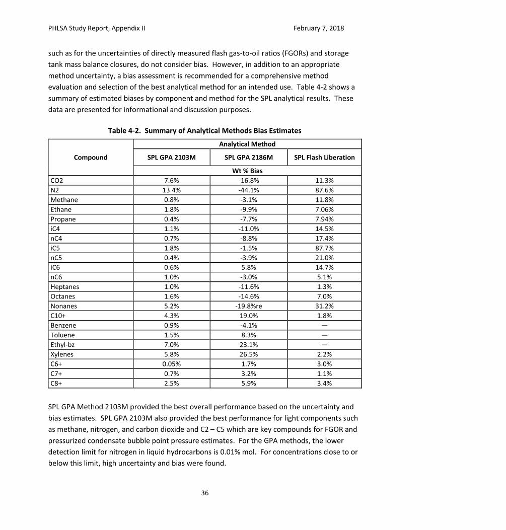
PHLSA Study Report, Appendix II February 7, 2018
36
such as for the uncertainties of directly measured flash gas-to-oil ratios (FGORs) and storage
tank mass balance closures, do not consider bias. However, in addition to an appropriate
method uncertainty, a bias assessment is recommended for a comprehensive method
evaluation and selection of the best analytical method for an intended use. Table 4-2 shows a
summary of estimated biases by component and method for the SPL analytical results. These
data are presented for informational and discussion purposes.
Table 4-2. Summary of Analytical Methods Bias Estimates
Compound
Analytical Method
SPL GPA 2103M SPL GPA 2186M SPL Flash Liberation
Wt % Bias
CO2 7.6% -16.8% 11.3%
N2 13.4% -44.1% 87.6%
Methane 0.8% -3.1% 11.8%
Ethane 1.8% -9.9% 7.06%
Propane 0.4% -7.7% 7.94%
iC4 1.1% -11.0% 14.5%
nC4 0.7% -8.8% 17.4%
iC5 1.8% -1.5% 87.7%
nC5 0.4% -3.9% 21.0%
iC6 0.6% 5.8% 14.7%
nC6 1.0% -3.0% 5.1%
Heptanes 1.0% -11.6% 1.3%
Octanes 1.6% -14.6% 7.0%
Nonanes 5.2% -19.8%re 31.2%
C10+ 4.3% 19.0% 1.8%
Benzene 0.9% -4.1% —
Toluene 1.5% 8.3% —
Ethyl-bz 7.0% 23.1% —
Xylenes 5.8% 26.5% 2.2%
C6+ 0.05% 1.7% 3.0%
C7+ 0.7% 3.2% 1.1%
C8+ 2.5% 5.9% 3.4%
SPL GPA Method 2103M provided the best overall performance based on the uncertainty and
bias estimates. SPL GPA 2103M also provided the best performance for light components such
as methane, nitrogen, and carbon dioxide and C2 – C5 which are key compounds for FGOR and
pressurized condensate bubble point pressure estimates. For the GPA methods, the lower
detection limit for nitrogen in liquid hydrocarbons is 0.01% mol. For concentrations close to or
below this limit, high uncertainty and bias were found.
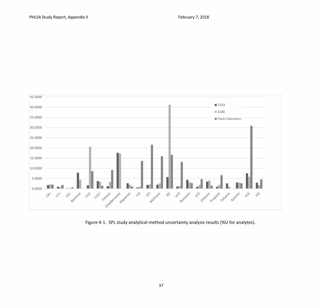
PHLSA Study Report, Appendix II February 7, 2018
37
0.0000
5.0000
10.0000
15.0000
20.0000
25.0000
30.0000
35.0000
40.0000
45.0000
2103
2186
Flash Liberation
Figure 4-1. SPL study analytical method uncertainty analysis results (%U for analytes).
PHLSA Study Report, Appendix II February 7, 2018
38
4.3 Weighted bias
The pressurized hydrocarbon analytical methods evaluated for this project were developed for
different applications (e.g., for NGLs (natural gas liquids), light and heavy condensates, or crude
oil), and the estimated bias of these methods will depend on the sample properties. The
impact of a method bias on an application (e.g., FGOR estimates) can be evaluated for the
individual components bias, as an average bias for all the components, and as a weighted
average bias. Weighed bias calculation is intended to assign more importance to components
with larger concentration than those with lower concentration. A component with a large bias
and lower concentration will have less impact on the overall results compared to a component
with a large concentration component with low bias.
The average bias of all components may provide a better indication whether an analytical
method is appropriate for the sample than the biases of the individual components. An
inappropriate analytical method will result in both high bias and uncertainty for certain
components, and a high average bias. Thus, a weighted bias calculation may be a better
indicator of the impact of the method bias on an application than the average bias. For a
weighted bias calculation, the biases of the most abundant components have larger weight in
the total bias calculated for the sample. Based on the example sample composition presented
in Table 4-3, Table 4-4 provides average and weighted bias estimates for the three SPL
pressurized hydrocarbons analytical methods, and shows that weighted bias estimates are
generally lower than average bias estimates. This is primarily because low concentration / high
bias components such as nitrogen and carbon dioxide have less impact on weighted bias
estimates.
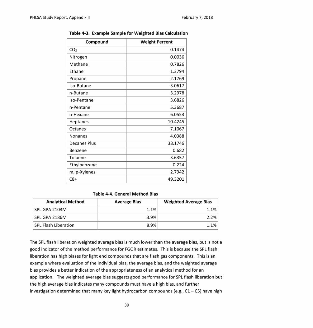
PHLSA Study Report, Appendix II February 7, 2018
39
Table 4-3. Example Sample for Weighted Bias Calculation
Compound Weight Percent
CO2 0.1474
Nitrogen 0.0036
Methane 0.7826
Ethane 1.3794
Propane 2.1769
Iso-Butane 3.0617
n-Butane 3.2978
Iso-Pentane 3.6826
n-Pentane 5.3687
n-Hexane 6.0553
Heptanes 10.4245
Octanes 7.1067
Nonanes 4.0388
Decanes Plus 38.1746
Benzene 0.682
Toluene 3.6357
Ethylbenzene 0.224
m, p-Xylenes 2.7942
C8+ 49.3201
Table 4-4. General Method Bias
Analytical Method Average Bias Weighted Average Bias
SPL GPA 2103M 1.1% 1.1%
SPL GPA 2186M 3.9% 2.2%
SPL Flash Liberation 8.9% 1.1%
The SPL flash liberation weighted average bias is much lower than the average bias, but is not a
good indicator of the method performance for FGOR estimates. This is because the SPL flash
liberation has high biases for light end compounds that are flash gas components. This is an
example where evaluation of the individual bias, the average bias, and the weighted average
bias provides a better indication of the appropriateness of an analytical method for an
application. The weighted average bias suggests good performance for SPL flash liberation but
the high average bias indicates many compounds must have a high bias, and further
investigation determined that many key light hydrocarbon compounds (e.g., C1 – C5) have high
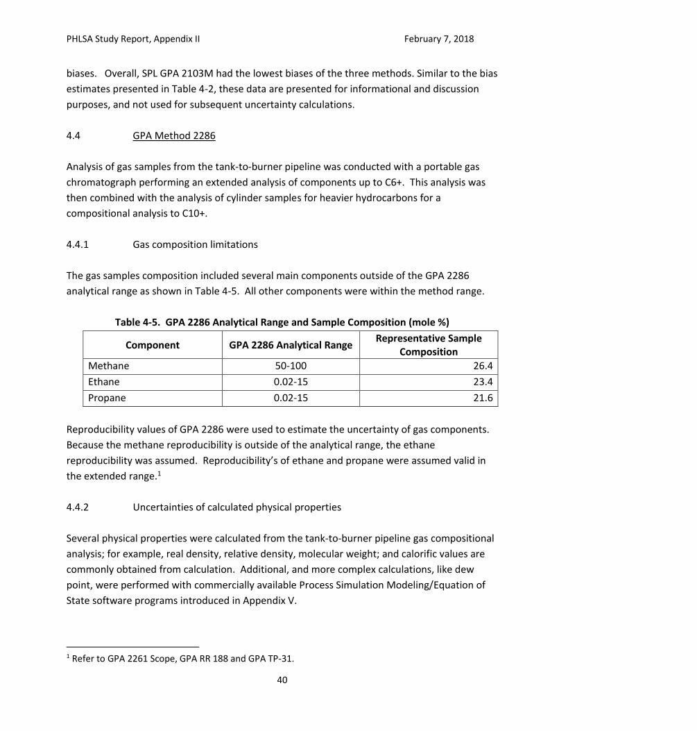
PHLSA Study Report, Appendix II February 7, 2018
40
biases. Overall, SPL GPA 2103M had the lowest biases of the three methods. Similar to the bias
estimates presented in Table 4-2, these data are presented for informational and discussion
purposes, and not used for subsequent uncertainty calculations.
4.4 GPA Method 2286
Analysis of gas samples from the tank-to-burner pipeline was conducted with a portable gas
chromatograph performing an extended analysis of components up to C6+. This analysis was
then combined with the analysis of cylinder samples for heavier hydrocarbons for a
compositional analysis to C10+.
4.4.1 Gas composition limitations
The gas samples composition included several main components outside of the GPA 2286
analytical range as shown in Table 4-5. All other components were within the method range.
Table 4-5. GPA 2286 Analytical Range and Sample Composition (mole %)
Component GPA 2286 Analytical Range Representative Sample
Composition
Methane 50-100 26.4
Ethane 0.02-15 23.4
Propane 0.02-15 21.6
Reproducibility values of GPA 2286 were used to estimate the uncertainty of gas components.
Because the methane reproducibility is outside of the analytical range, the ethane
reproducibility was assumed. Reproducibility’s of ethane and propane were assumed valid in
the extended range.1
4.4.2 Uncertainties of calculated physical properties
Several physical properties were calculated from the tank-to-burner pipeline gas compositional
analysis; for example, real density, relative density, molecular weight; and calorific values are
commonly obtained from calculation. Additional, and more complex calculations, like dew
point, were performed with commercially available Process Simulation Modeling/Equation of
State software programs introduced in Appendix V.
1 Refer to GPA 2261 Scope, GPA RR 188 and GPA TP-31.
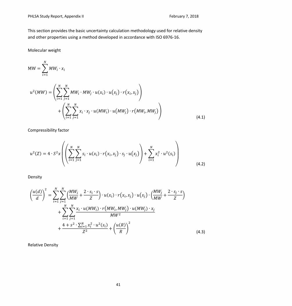
PHLSA Study Report, Appendix II February 7, 2018
41
This section provides the basic uncertainty calculation methodology used for relative density
and other properties using a method developed in accordance with ISO 6976-16.
Molecular weight
MW = ∑𝑀𝑊𝑖 ∙ 𝑥𝑖
𝑁
𝑖=1
𝑢2(𝑀𝑊) = (∑∑𝑀𝑊𝑖 ∙ 𝑀𝑊𝑗 ∙ 𝑢(𝑥𝑖) ∙ 𝑢(𝑥𝑗) ∙ 𝑟(𝑥𝑖 , 𝑥𝑗)
𝑁
𝑗=1
𝑁
𝑖=1
)
+ (∑∑𝑥𝑖 ∙ 𝑥𝑗 ∙ 𝑢(𝑀𝑊𝑖) ∙ 𝑢(𝑀𝑊𝑗) ∙ 𝑟(𝑀𝑊𝑖, 𝑀𝑊𝑗)
𝑁
𝑗=1
𝑁
𝑖=1
)
(4.1)
Compressibility factor
𝑢2(𝑍) = 4 ∙ 𝑆2𝑥
(
(∑∑𝑠𝑖 ∙ 𝑢(𝑥𝑖) ∙ 𝑟(𝑥𝑖 , 𝑥𝑗)
𝑁
𝑗=1
𝑁
𝑖=1
∙ 𝑠𝑗 ∙ 𝑢(𝑥𝑗)) + ∑𝑥𝑖2 ∙ 𝑢2(𝑠𝑖)
𝑁
𝑖=1
)
(4.2)
Density
(𝑢(𝑑)
𝑑)
2
= ∑∑(𝑀𝑊𝑖
𝑀𝑊+
2 ∙ 𝑠𝑖 ∙ 𝑠
𝑍) ∙ 𝑢(𝑥𝑖) ∙ 𝑟(𝑥𝑖, 𝑥𝑗) ∙ 𝑢(𝑥𝑗) ∙ (
𝑀𝑊𝑗
𝑀𝑊+
2 ∙ 𝑠𝑗 ∙ 𝑠
𝑍)
𝑁
𝑗=1
𝑁
𝑖=1
+ ∑∑𝑥𝑖 ∙ 𝑢(𝑀𝑊𝑖) ∙ 𝑟(𝑀𝑊𝑖, 𝑀𝑊𝑗) ∙ 𝑢(𝑀𝑊𝑗) ∙ 𝑥𝑗
𝑀𝑊2
𝑁
𝑗=1
𝑁
𝑖=1
+4 + 𝑠2 ∙ ∑ 𝑥𝑖
2 ∙ 𝑢2(𝑠𝑖)𝑁𝑖=1
𝑍2+ (
𝑢(𝑅)
𝑅)
2
(4.3)
Relative Density
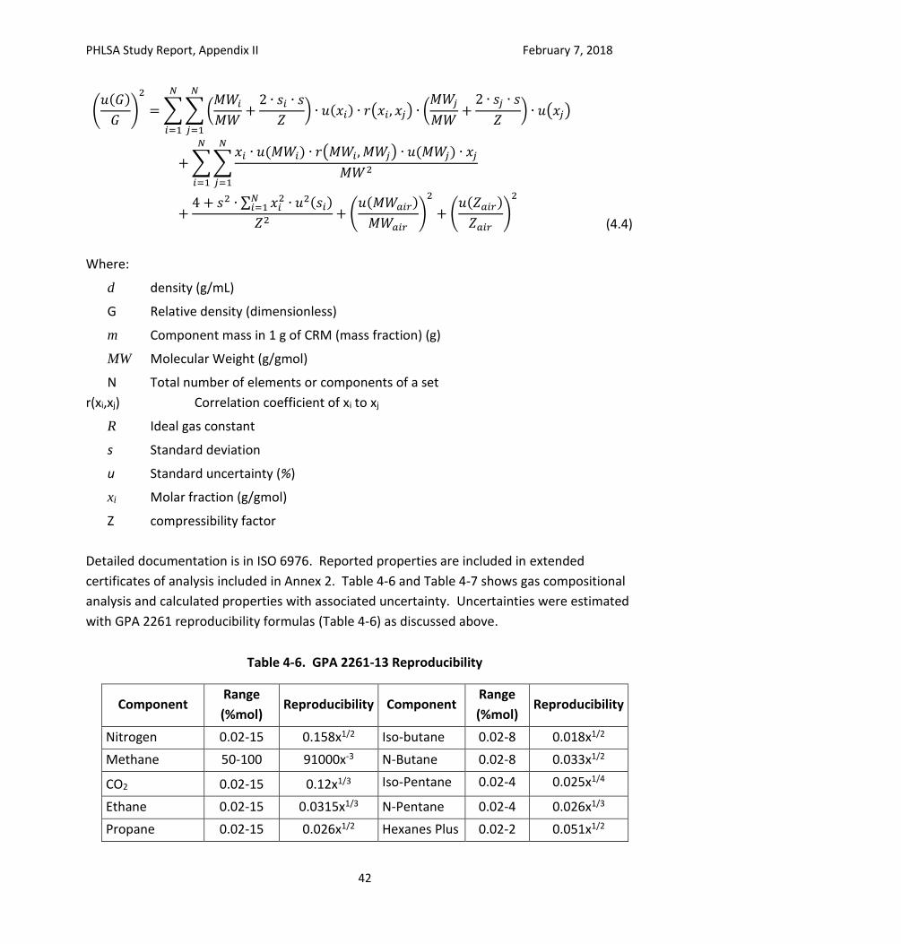
PHLSA Study Report, Appendix II February 7, 2018
42
(𝑢(𝐺)
𝐺)
2
= ∑∑(𝑀𝑊𝑖
𝑀𝑊+
2 ∙ 𝑠𝑖 ∙ 𝑠
𝑍) ∙ 𝑢(𝑥𝑖) ∙ 𝑟(𝑥𝑖, 𝑥𝑗) ∙ (
𝑀𝑊𝑗
𝑀𝑊+
2 ∙ 𝑠𝑗 ∙ 𝑠
𝑍) ∙ 𝑢(𝑥𝑗)
𝑁
𝑗=1
𝑁
𝑖=1
+ ∑∑𝑥𝑖 ∙ 𝑢(𝑀𝑊𝑖) ∙ 𝑟(𝑀𝑊𝑖, 𝑀𝑊𝑗) ∙ 𝑢(𝑀𝑊𝑗) ∙ 𝑥𝑗
𝑀𝑊2
𝑁
𝑗=1
𝑁
𝑖=1
+4 + 𝑠2 ∙ ∑ 𝑥𝑖
2 ∙ 𝑢2(𝑠𝑖)𝑁𝑖=1
𝑍2+ (
𝑢(𝑀𝑊𝑎𝑖𝑟)
𝑀𝑊𝑎𝑖𝑟)
2
+ (𝑢(𝑍𝑎𝑖𝑟)
𝑍𝑎𝑖𝑟)
2
(4.4)
Where:
d density (g/mL)
G Relative density (dimensionless)
m Component mass in 1 g of CRM (mass fraction) (g)
MW Molecular Weight (g/gmol)
N Total number of elements or components of a set
r(xi,xj) Correlation coefficient of xi to xj
R Ideal gas constant
s Standard deviation
u Standard uncertainty (%)
xi Molar fraction (g/gmol)
Z compressibility factor
Detailed documentation is in ISO 6976. Reported properties are included in extended
certificates of analysis included in Annex 2. Table 4-6 and Table 4-7 shows gas compositional
analysis and calculated properties with associated uncertainty. Uncertainties were estimated
with GPA 2261 reproducibility formulas (Table 4-6) as discussed above.
Table 4-6. GPA 2261-13 Reproducibility
Component Range
(%mol) Reproducibility Component
Range
(%mol) Reproducibility
Nitrogen 0.02-15 0.158x1/2 Iso-butane 0.02-8 0.018x1/2
Methane 50-100 91000x-3 N-Butane 0.02-8 0.033x1/2
CO2 0.02-15 0.12x1/3 Iso-Pentane 0.02-4 0.025x1/4
Ethane 0.02-15 0.0315x1/3 N-Pentane 0.02-4 0.026x1/3
Propane 0.02-15 0.026x1/2 Hexanes Plus 0.02-2 0.051x1/2
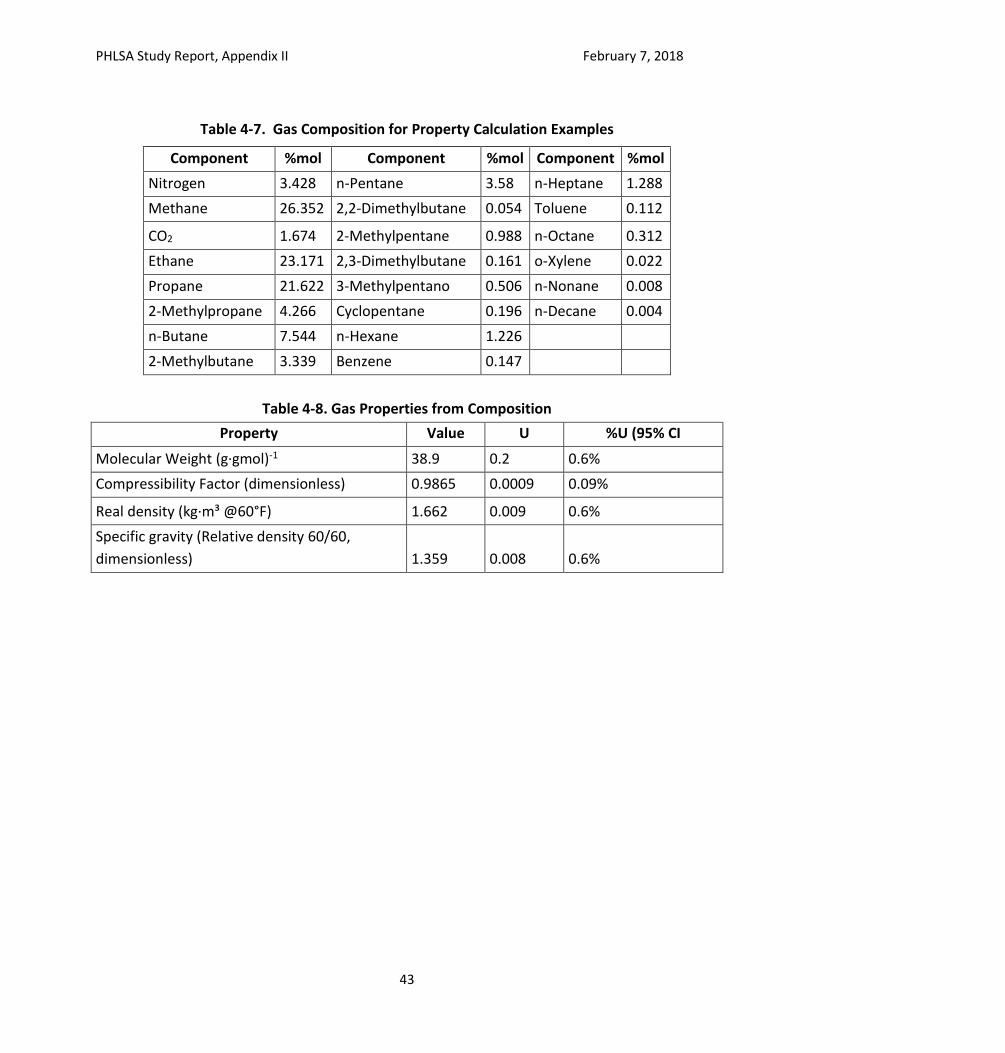
PHLSA Study Report, Appendix II February 7, 2018
43
Table 4-7. Gas Composition for Property Calculation Examples
Component %mol Component %mol Component %mol
Nitrogen 3.428 n-Pentane 3.58 n-Heptane 1.288
Methane 26.352 2,2-Dimethylbutane 0.054 Toluene 0.112
CO2 1.674 2-Methylpentane 0.988 n-Octane 0.312
Ethane 23.171 2,3-Dimethylbutane 0.161 o-Xylene 0.022
Propane 21.622 3-Methylpentano 0.506 n-Nonane 0.008
2-Methylpropane 4.266 Cyclopentane 0.196 n-Decane 0.004
n-Butane 7.544 n-Hexane 1.226 2-Methylbutane 3.339 Benzene 0.147
Table 4-8. Gas Properties from Composition
Property Value U %U (95% CI
Molecular Weight (g·gmol)-1 38.9 0.2 0.6%
Compressibility Factor (dimensionless) 0.9865 0.0009 0.09%
Real density (kg·m³ @60°F) 1.662 0.009 0.6%
Specific gravity (Relative density 60/60,
dimensionless) 1.359 0.008 0.6%
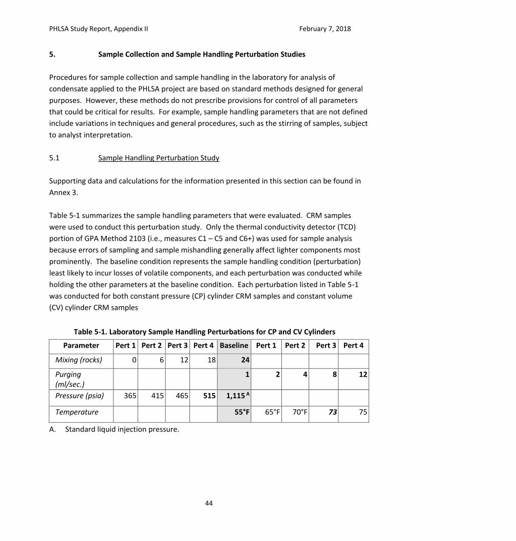
PHLSA Study Report, Appendix II February 7, 2018
44
5. Sample Collection and Sample Handling Perturbation Studies
Procedures for sample collection and sample handling in the laboratory for analysis of
condensate applied to the PHLSA project are based on standard methods designed for general
purposes. However, these methods do not prescribe provisions for control of all parameters
that could be critical for results. For example, sample handling parameters that are not defined
include variations in techniques and general procedures, such as the stirring of samples, subject
to analyst interpretation.
5.1 Sample Handling Perturbation Study
Supporting data and calculations for the information presented in this section can be found in
Annex 3.
Table 5-1 summarizes the sample handling parameters that were evaluated. CRM samples
were used to conduct this perturbation study. Only the thermal conductivity detector (TCD)
portion of GPA Method 2103 (i.e., measures C1 – C5 and C6+) was used for sample analysis
because errors of sampling and sample mishandling generally affect lighter components most
prominently. The baseline condition represents the sample handling condition (perturbation)
least likely to incur losses of volatile components, and each perturbation was conducted while
holding the other parameters at the baseline condition. Each perturbation listed in Table 5-1
was conducted for both constant pressure (CP) cylinder CRM samples and constant volume
(CV) cylinder CRM samples
Table 5-1. Laboratory Sample Handling Perturbations for CP and CV Cylinders
Parameter Pert 1 Pert 2 Pert 3 Pert 4 Baseline Pert 1 Pert 2 Pert 3 Pert 4
Mixing (rocks) 0 6 12 18 24
Purging (ml/sec.)
1 2 4 8 12
Pressure (psia) 365 415 465 515 1,115 A
Temperature
55°F 65°F 70°F 73 75
A. Standard liquid injection pressure.
PHLSA Study Report, Appendix II February 7, 2018
45
ASTM E1169 “Standard Practice for Conducting Ruggedness Tests” provides tools for assessing
the statistical significance of a method parameter (e.g., sample temperature, sample
mixing) “effect” over method outcomes. In this discussion, some concepts of ASTM E1169
will be used:
- Ruggedness; the insensitivity of a test method to departures from specified test or
environmental conditions.
- Factor: a test parameter that may affect either the result obtained from the use of a test
method or the variability of that result.
- Effect: the impact of a factor (method parameter) change upon analytical results.
The effect of a method parameter on analytical results for individual sample components does
not necessarily represent the effect of the method parameter over analytical results for
composite sample properties. To assess the combined effects of method parameters, the
vapor pressure by Raoult's Law was calculated and included in the evaluation.
The ruggedness test procedure consists of the following steps:
- Identification of relevant factors;
- Base line condition definition;
- Selection of appropriate levels to be used in experiment runs;
- Execution of runs in a random order;
- Calculation of High and Low level factors and results from experimental data;
- Statistical analysis to determine the effect of factors on the test method results; and
- Results revision and conclusions
The experimental design shown in Table 5-1 includes more experiments than high and low
conditions, and a modification of the ASTM method was needed in order to obtain only two
levels. For example, for the mixing factor, with perturbations of 0, 6, 12, 18, and 24 rocks, the
low condition factor was assumed to be the average of 0 and 6 rocks and the high condition
factor was assumed to be the average of 18 and 24 rocks.
Because the effect of each factor was isolated (i.e., only one factor was changed for each
perturbation), there were no factor interactions and direct determination of the effect of each
factor was possible. This exceeds the experimental design requirements of ASTM E1169. Also,
PHLSA Study Report, Appendix II February 7, 2018
46
the number of data points is six to ten times larger than the ASTM method requirements, and
the larger data set produces a more robust result.
The statistical significance of a factor is determined by comparing the standard deviation of
effect differences caused by changing the factor and the standard deviation of the effect
differences from the entire set of factor change experiments.
A half-normal plot is used to present potentially statistical significant factors. Plot construction
steps are:
Construct a results table with analytical results differences against baseline condition result,
these data will be at abscissa axis (i.e., x values);
Sort absolute differences in decreasing order;
Ordinates are standard deviations as indicated by ASTM D1169 Table A2.1 or can be
calculated applying the normal probability: Φ-1(0.5+0.5[e - 0.5]/E) (ASTM E1169 − 14
A2.1), excel formula is "=INV.NORM(0.5+0.5*(e-0.5)/E,0,1)" where E is the number of
Effects, e is the increasing number from 1 to E, and Φ(x) is the probability that the
standard normal distribution gives a value less than x. Values for five factors correspond
to 0.126, 0.385, 0.674, 1.036 and 1.645;
Calculate one standard deviation for the full data set of differences;
Plot the standard deviation as solid line up to 2 standard deviations and plot parameter
(factors) differences as dots.
Half normal plot interpretation: Method parameters (factors) with greater impact on analytical
results are further from the origin than method parameters with lower impact on analytical
results. The straight line represents one standard deviation. Method parameters with statistical
significant difference are far from the line.
5.1.1 Ruggedness Test Calculations
Conducting a ruggedness test is based on making systematic changes to method parameters,
called factors in the ASTM method, and then observing associated effects upon each test result.
Factors are features of the test method or of the laboratory environment that can vary across
laboratories and can impact the method outcome.
Perturbation factors chosen for ruggedness testing are those believed to have potential to
affect results. Identified perturbation factors and corresponding change values listed in Table 5-
PHLSA Study Report, Appendix II February 7, 2018
47
1 were performed isolated from other factors; that is, other factors were maintained at the
most conservative sample handling condition (base line condition): mixing (24 rocks), pressure
(1,100 psig), temperature (55 °F) and purge rate (1 ml/min), and CP sample cylinder.
A statistical analysis to determine the impact of perturbation factors on test method results
was conducted and is summarized in section 5.1.5. Possible revisions to the test method and
specific guidelines to follow to optimize analytical results are discussed in conclusions.
The standard deviation of the method parameter/factor impact on analytical results was
calculated as a pooled standard deviation (ASTM D1169 eq. 1):
𝑠 =∑(𝑥𝑖 − �̅�)
𝑛 − 1
𝑠𝑝 = √(𝑛1 − 1)𝑠1
2 + (𝑛2 − 1)𝑠22 + ⋯+ (𝑛𝑛 − 1)𝑠𝑘
2
𝑛1 + 𝑛2 + ⋯+ 𝑛𝑘 − 𝑘
𝑠𝑒𝑓𝑓 = √4𝑠𝑝
2
𝑛
(5.1)
𝑡 =|𝑒𝑓𝑓𝑒𝑐𝑡 𝑑𝑖𝑓𝑓𝑒𝑟𝑒𝑛𝑐𝑒|
𝑠𝑒𝑓𝑓
(5.2)
Where:
s Standard deviation
n Number of runs or data
xi Analytical result
N Number of effects in the array
r Number of replicates of the effect
k Degrees of freedom = Number of data sets (i.e., number of factors)
sp Pooled standard deviation
seff Estimated standard deviation of test result
t Critical value of t distribution
The student t value was calculated by dividing the absolute value of effect difference by seff and
the probability of the t score was based on two tails and (Number of effects-1)(replicates-1)
degrees of freedom.
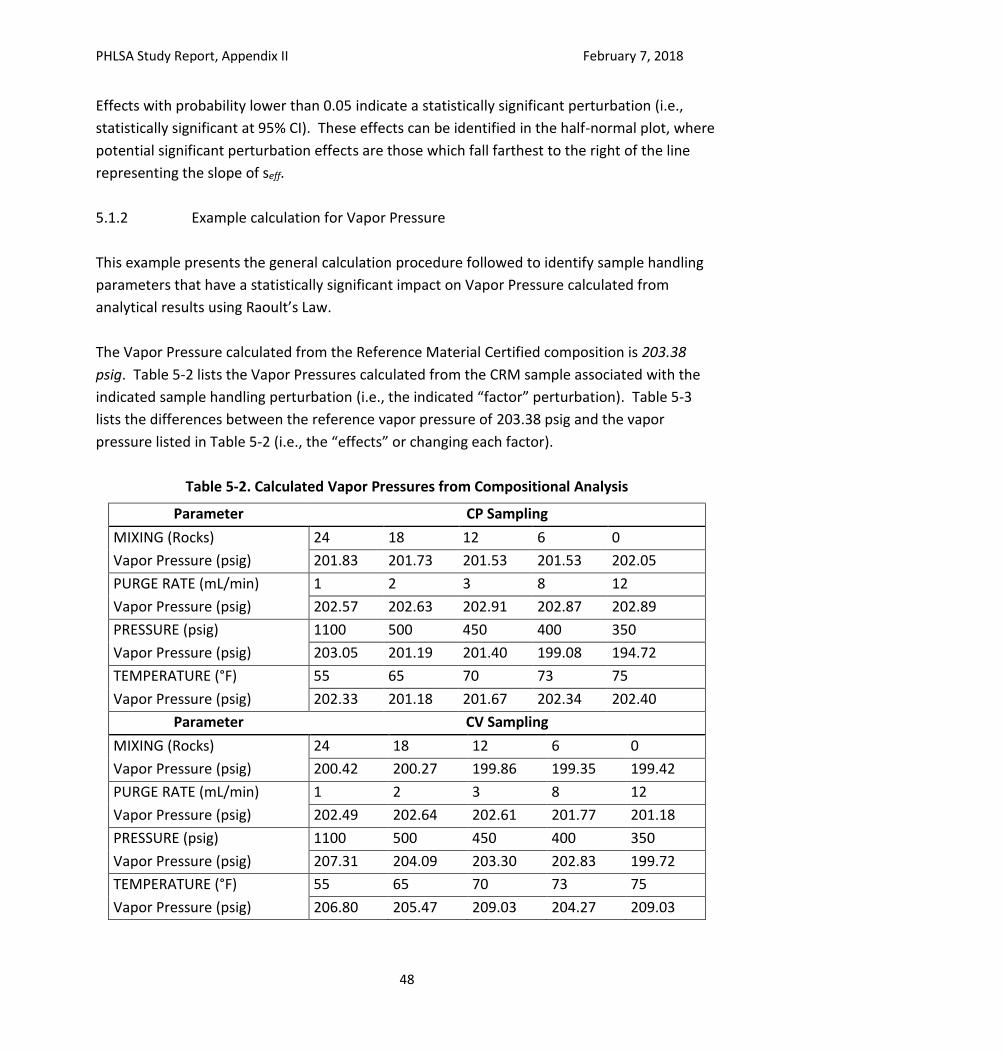
PHLSA Study Report, Appendix II February 7, 2018
48
Effects with probability lower than 0.05 indicate a statistically significant perturbation (i.e.,
statistically significant at 95% CI). These effects can be identified in the half-normal plot, where
potential significant perturbation effects are those which fall farthest to the right of the line
representing the slope of seff.
5.1.2 Example calculation for Vapor Pressure
This example presents the general calculation procedure followed to identify sample handling
parameters that have a statistically significant impact on Vapor Pressure calculated from
analytical results using Raoult’s Law.
The Vapor Pressure calculated from the Reference Material Certified composition is 203.38
psig. Table 5-2 lists the Vapor Pressures calculated from the CRM sample associated with the
indicated sample handling perturbation (i.e., the indicated “factor” perturbation). Table 5-3
lists the differences between the reference vapor pressure of 203.38 psig and the vapor
pressure listed in Table 5-2 (i.e., the “effects” or changing each factor).
Table 5-2. Calculated Vapor Pressures from Compositional Analysis
Parameter CP Sampling
MIXING (Rocks) 24 18 12 6 0
Vapor Pressure (psig) 201.83 201.73 201.53 201.53 202.05
PURGE RATE (mL/min) 1 2 3 8 12
Vapor Pressure (psig) 202.57 202.63 202.91 202.87 202.89
PRESSURE (psig) 1100 500 450 400 350
Vapor Pressure (psig) 203.05 201.19 201.40 199.08 194.72
TEMPERATURE (°F) 55 65 70 73 75
Vapor Pressure (psig) 202.33 201.18 201.67 202.34 202.40
Parameter CV Sampling
MIXING (Rocks) 24 18 12 6 0
Vapor Pressure (psig) 200.42 200.27 199.86 199.35 199.42
PURGE RATE (mL/min) 1 2 3 8 12
Vapor Pressure (psig) 202.49 202.64 202.61 201.77 201.18
PRESSURE (psig) 1100 500 450 400 350
Vapor Pressure (psig) 207.31 204.09 203.30 202.83 199.72
TEMPERATURE (°F) 55 65 70 73 75
Vapor Pressure (psig) 206.80 205.47 209.03 204.27 209.03
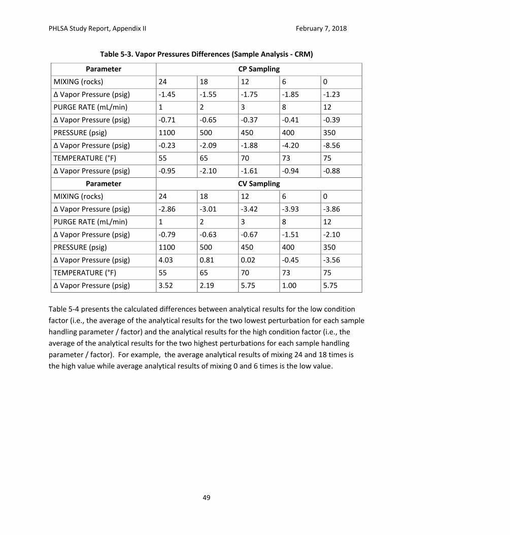
PHLSA Study Report, Appendix II February 7, 2018
49
Table 5-3. Vapor Pressures Differences (Sample Analysis - CRM)
Parameter CP Sampling
MIXING (rocks) 24 18 12 6 0
Δ Vapor Pressure (psig) -1.45 -1.55 -1.75 -1.85 -1.23
PURGE RATE (mL/min) 1 2 3 8 12
Δ Vapor Pressure (psig) -0.71 -0.65 -0.37 -0.41 -0.39
PRESSURE (psig) 1100 500 450 400 350
Δ Vapor Pressure (psig) -0.23 -2.09 -1.88 -4.20 -8.56
TEMPERATURE (°F) 55 65 70 73 75
Δ Vapor Pressure (psig) -0.95 -2.10 -1.61 -0.94 -0.88
Parameter CV Sampling
MIXING (rocks) 24 18 12 6 0
Δ Vapor Pressure (psig) -2.86 -3.01 -3.42 -3.93 -3.86
PURGE RATE (mL/min) 1 2 3 8 12
Δ Vapor Pressure (psig) -0.79 -0.63 -0.67 -1.51 -2.10
PRESSURE (psig) 1100 500 450 400 350
Δ Vapor Pressure (psig) 4.03 0.81 0.02 -0.45 -3.56
TEMPERATURE (°F) 55 65 70 73 75
Δ Vapor Pressure (psig) 3.52 2.19 5.75 1.00 5.75
Table 5-4 presents the calculated differences between analytical results for the low condition
factor (i.e., the average of the analytical results for the two lowest perturbation for each sample
handling parameter / factor) and the analytical results for the high condition factor (i.e., the
average of the analytical results for the two highest perturbations for each sample handling
parameter / factor). For example, the average analytical results of mixing 24 and 18 times is
the high value while average analytical results of mixing 0 and 6 times is the low value.
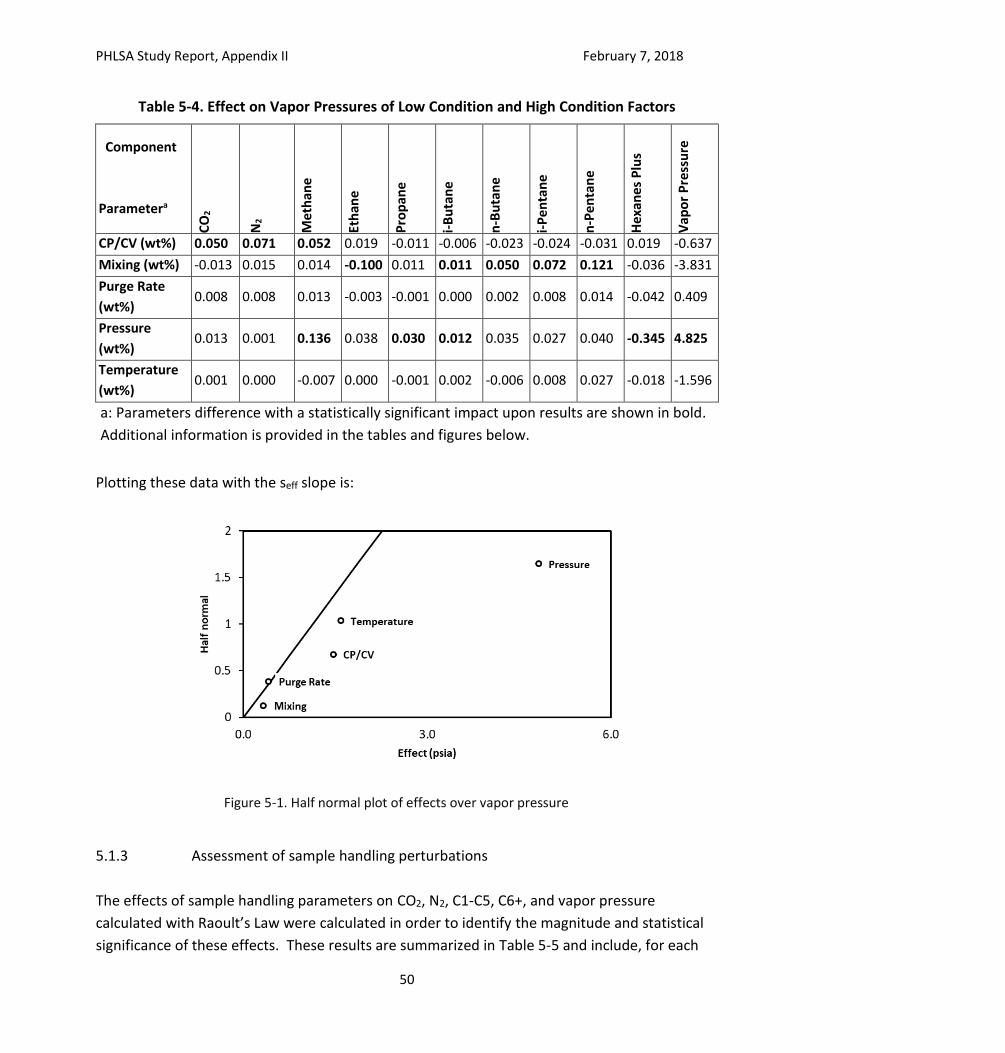
PHLSA Study Report, Appendix II February 7, 2018
50
Table 5-4. Effect on Vapor Pressures of Low Condition and High Condition Factors
Component
Parametera C
O2
N2
Met
han
e
Eth
ane
Pro
pan
e
i-B
uta
ne
n-B
uta
ne
i-P
en
tan
e
n-P
en
tan
e
Hex
anes
Plu
s
Vap
or
Pre
ssu
re
CP/CV (wt%) 0.050 0.071 0.052 0.019 -0.011 -0.006 -0.023 -0.024 -0.031 0.019 -0.637
Mixing (wt%) -0.013 0.015 0.014 -0.100 0.011 0.011 0.050 0.072 0.121 -0.036 -3.831
Purge Rate
(wt%) 0.008 0.008 0.013 -0.003 -0.001 0.000 0.002 0.008 0.014 -0.042 0.409
Pressure
(wt%) 0.013 0.001 0.136 0.038 0.030 0.012 0.035 0.027 0.040 -0.345 4.825
Temperature
(wt%) 0.001 0.000 -0.007 0.000 -0.001 0.002 -0.006 0.008 0.027 -0.018 -1.596
a: Parameters difference with a statistically significant impact upon results are shown in bold.
Additional information is provided in the tables and figures below.
Plotting these data with the seff slope is:
5.1.3 Assessment of sample handling perturbations
The effects of sample handling parameters on CO2, N2, C1-C5, C6+, and vapor pressure
calculated with Raoult’s Law were calculated in order to identify the magnitude and statistical
significance of these effects. These results are summarized in Table 5-5 and include, for each
Figure 5-1. Half normal plot of effects over vapor pressure
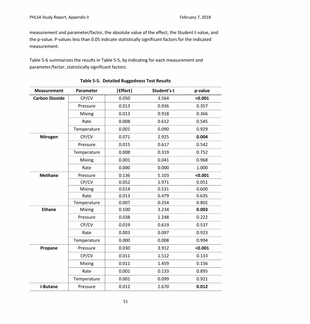
PHLSA Study Report, Appendix II February 7, 2018
51
measurement and parameter/factor, the absolute value of the effect, the Student t-value, and
the p-value. P-values less than 0.05 indicate statistically significant factors for the indicated
measurement.
Table 5-6 summarizes the results in Table 5-5, by indicating for each measurement and
parameter/factor, statistically significant factors.
Table 5-5. Detailed Ruggedness Test Results
Measurement Parameter |Effect| Student's t p-value
Carbon Dioxide CP/CV 0.050 3.564 <0.001
Pressure 0.013 0.936 0.357
Mixing 0.013 0.918 0.366
Rate 0.008 0.612 0.545
Temperature 0.001 0.090 0.929
Nitrogen CP/CV 0.071 2.925 0.004
Pressure 0.015 0.617 0.542
Temperature 0.008 0.319 0.752
Mixing 0.001 0.041 0.968
Rate 0.000 0.000 1.000
Methane Pressure 0.136 5.103 <0.001
CP/CV 0.052 1.971 0.051
Mixing 0.014 0.531 0.600
Rate 0.013 0.479 0.635
Temperature 0.007 0.254 0.802
Ethane Mixing 0.100 3.234 0.003
Pressure 0.038 1.248 0.222
CP/CV 0.019 0.619 0.537
Rate 0.003 0.097 0.923
Temperature 0.000 0.008 0.994
Propane Pressure 0.030 3.912 <0.001
CP/CV 0.011 1.512 0.133
Mixing 0.011 1.459 0.156
Rate 0.001 0.133 0.895
Temperature 0.001 0.099 0.921
i-Butane Pressure 0.012 2.670 0.012
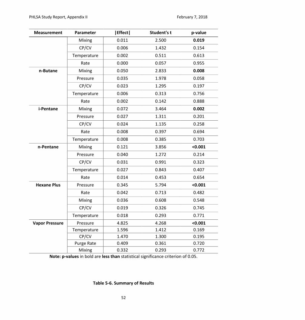
PHLSA Study Report, Appendix II February 7, 2018
52
Measurement Parameter |Effect| Student's t p-value
Mixing 0.011 2.500 0.019
CP/CV 0.006 1.432 0.154
Temperature 0.002 0.511 0.613
Rate 0.000 0.057 0.955
n-Butane Mixing 0.050 2.833 0.008
Pressure 0.035 1.978 0.058
CP/CV 0.023 1.295 0.197
Temperature 0.006 0.313 0.756
Rate 0.002 0.142 0.888
i-Pentane Mixing 0.072 3.464 0.002
Pressure 0.027 1.311 0.201
CP/CV 0.024 1.135 0.258
Rate 0.008 0.397 0.694
Temperature 0.008 0.385 0.703
n-Pentane Mixing 0.121 3.856 <0.001
Pressure 0.040 1.272 0.214
CP/CV 0.031 0.991 0.323
Temperature 0.027 0.843 0.407
Rate 0.014 0.453 0.654
Hexane Plus Pressure 0.345 5.794 <0.001
Rate 0.042 0.713 0.482
Mixing 0.036 0.608 0.548
CP/CV 0.019 0.326 0.745
Temperature 0.018 0.293 0.771
Vapor Pressure Pressure 4.825 4.268 <0.001
Temperature 1.596 1.412 0.169
CP/CV 1.470 1.300 0.195
Purge Rate 0.409 0.361 0.720
Mixing 0.332 0.293 0.772
Note: p-values in bold are less than statistical significance criterion of 0.05.
Table 5-6. Summary of Results
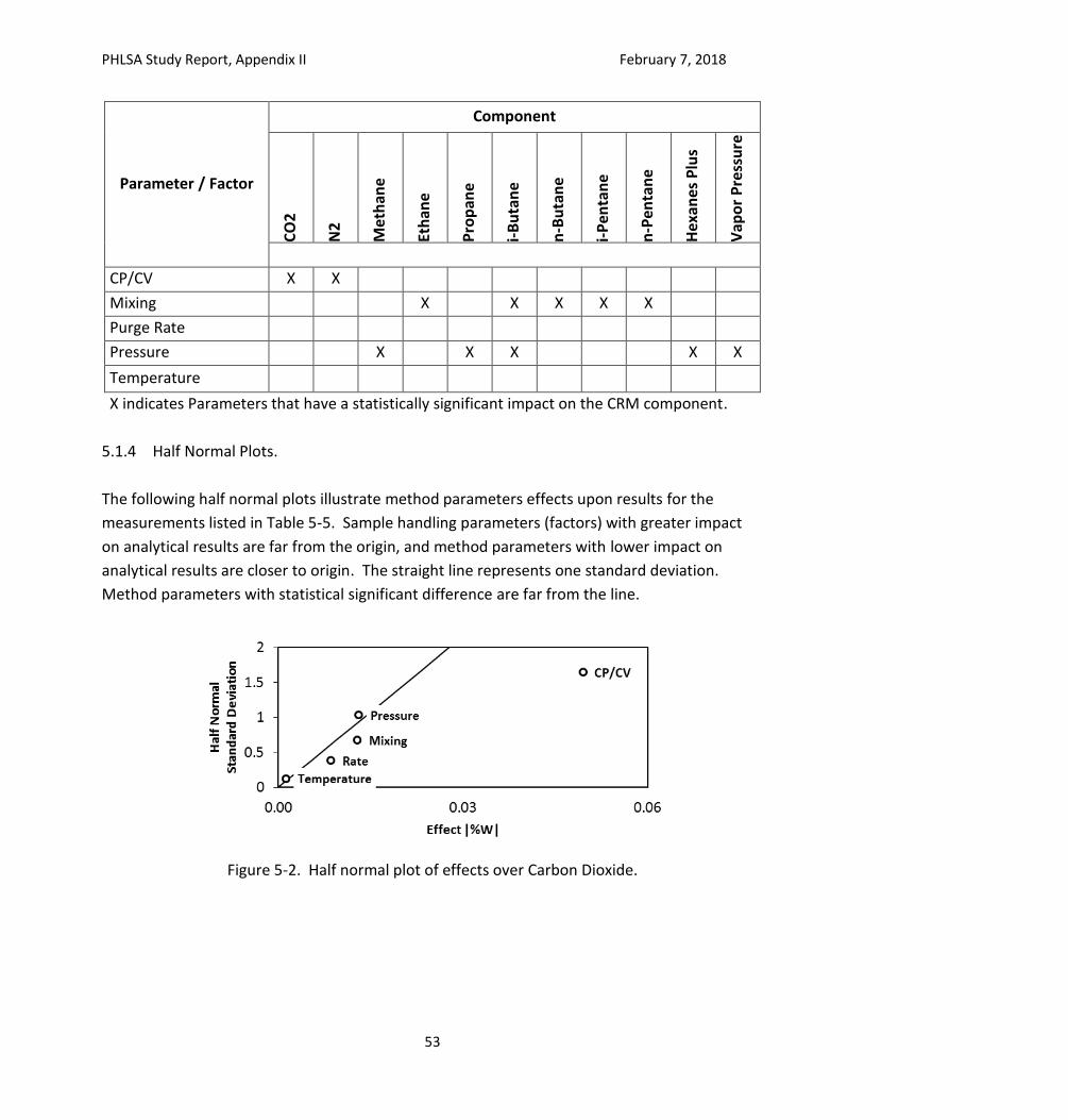
PHLSA Study Report, Appendix II February 7, 2018
53
Parameter / Factor
Component
CO
2
N2
Met
han
e
Eth
ane
Pro
pan
e
i-B
uta
ne
n-B
uta
ne
i-P
enta
ne
n-P
enta
ne
Hex
anes
Plu
s
Vap
or
Pre
ssu
re
CP/CV X X
Mixing X X X X X
Purge Rate
Pressure X X X X X
Temperature
X indicates Parameters that have a statistically significant impact on the CRM component.
5.1.4 Half Normal Plots.
The following half normal plots illustrate method parameters effects upon results for the
measurements listed in Table 5-5. Sample handling parameters (factors) with greater impact
on analytical results are far from the origin, and method parameters with lower impact on
analytical results are closer to origin. The straight line represents one standard deviation.
Method parameters with statistical significant difference are far from the line.
Figure 5-2. Half normal plot of effects over Carbon Dioxide.
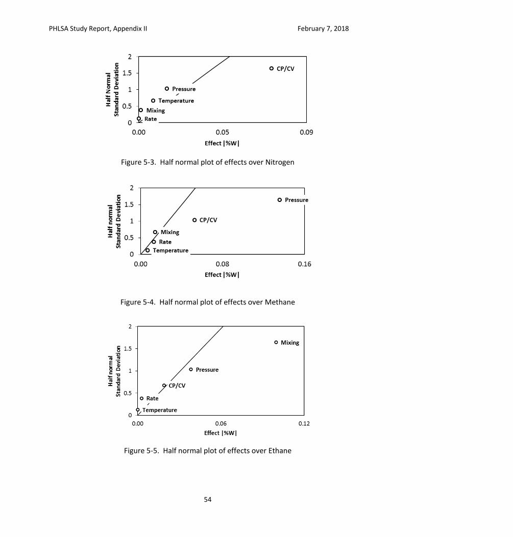
PHLSA Study Report, Appendix II February 7, 2018
54
Figure 5-3. Half normal plot of effects over Nitrogen
Figure 5-4. Half normal plot of effects over Methane
Figure 5-5. Half normal plot of effects over Ethane
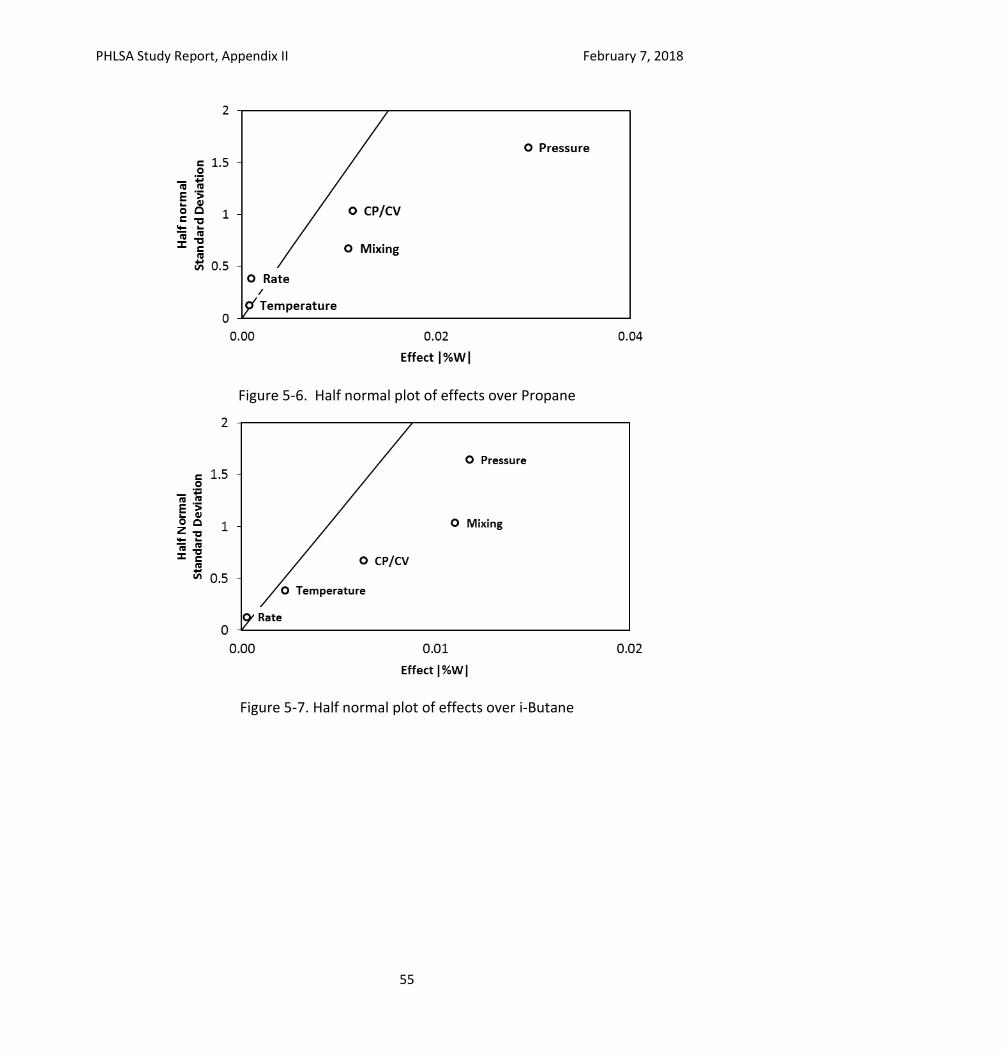
PHLSA Study Report, Appendix II February 7, 2018
55
Figure 5-6. Half normal plot of effects over Propane
Figure 5-7. Half normal plot of effects over i-Butane
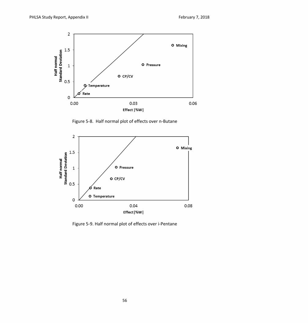
PHLSA Study Report, Appendix II February 7, 2018
56
Figure 5-8. Half normal plot of effects over n-Butane
Figure 5-9. Half normal plot of effects over i-Pentane
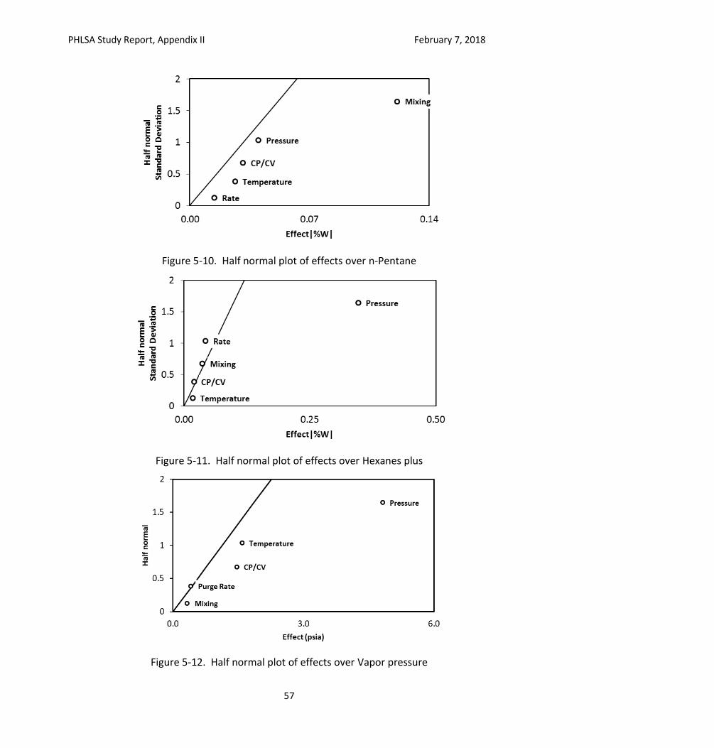
PHLSA Study Report, Appendix II February 7, 2018
57
Figure 5-10. Half normal plot of effects over n-Pentane
Figure 5-11. Half normal plot of effects over Hexanes plus
Figure 5-12. Half normal plot of effects over Vapor pressure
PHLSA Study Report, Appendix II February 7, 2018
58
5.1.5 Conclusions on sample handling perturbations
- The statistical analysis indicates that the sample handling parameters cylinder pre-
charge pressure and number of mixing rocks impact the analytical results for
compounds in the pressurized condensate samples. However, there is insufficient
statistical evidence to conclude that purge rate and sample temperature have influence
over the analytical results of tested samples.
- Sample collection cylinder type (constant pressure cylinder or two valve constant
volume cylinder) influences the light end compounds nitrogen and carbon dioxide.
- In order to avoid losses of volatile components, it is recommended that the pressure
applied to pre- charge should be a minimum of 300 psi above the simple collection
pressure. GPA 2174 guidelines recommend that the pre-charge sample pressure be a
minimum of 200 psi greater than the sample vapor pressure at injection valve
temperature. The number of rocks for sample homogenization should be between 18
and 24.
5.2 Sample Collection Perturbation Study
This task collected data to evaluate the impact of key sample collection parameters on
pressurized liquid HC sampling and analysis results to develop recommendations for sample
collection procedures. Parameters evaluated were:
Sample cylinder type (constant pressure (CP) cylinder and constant volume (CV) cylinder)
- Note that Section 5.1 evaluated laboratory sample handling parameters using lab-
prepared CRM samples in CP cylinders and CV cylinders, and compared analytical results
for these samples. This section evaluates analytical results of CP and CV cylinder
samples simultaneously collected from the test facility separator from adjacent sample
probes.
Sample collection rate (20, 40, 60, 100, and 180 ml/min)
Sample collection initiation time after the end of the well cycle (< 0, < 30, 90, and 150
minutes after well cycle). The well cycle is assumed to start when fluids first begin to flow
from the well to the separator and is assumed to end after the last separator-to-tank liquids
dump.
Sample collection location (sample probe and oil box oil level sight glass)
PHLSA Study Report, Appendix II February 7, 2018
59
Sample collection perturbations were primarily evaluated by comparing bubble point pressure
(PBP) / separator pressure during sample collection (Psc) ratios for all samples. Bubble point
pressures (at the sample collection temperature) were calculated by PSM/EOS from the
measured pressurized condensate composition, with PBP / Psc ratios greatly deviating from 1.0
being indicative of possible sample collection bias. Operational performance checks (OPC) data
analysis and discussion that follow show that PBP is very sensitive to methane and nitrogen (i.e.,
air) in condensate samples, and that samples that lose some methane or have some air
contamination may have anomalous PBP/PSC, but still provide reasonable estimates of flash gas
volume and composition. Thus, PBP/PSC is likely a very conservative OPC for sample collection
and analysis results.
Supporting data and calculations for the data tables and figures in this section are in the
following Excel document in Appendix VI:
PHLSA Study Task 8 Sample Collection Data.xlsm
GPA 2103 analytical results with the nitrogen mathematically removed were used for these
evaluations.
5.2.1 Sample cylinder type perturbation study
Overview of data collected and data analysis approach
Paired CV cylinder and CP cylinder pressurized condensate samples were simultaneously
collected during sampling events throughout the project using probe 1 and probe 3. The CV
and CP cylinders were randomly switched between probe 1 and probe 3 to address possible
sample probe bias. The samples were analyzed using GPA 2103M and GPA 2186M.
Paired CP cylinder /CV cylinder pressurized condensate samples data were evaluated using the
following steps to determine if there were statistically significant differences between the
sample collection methods during the PHLSA study.
A. Initial paired data comparisons t-statistic test. A paired data comparisons test was initially
used as a screening tool to determine whether CP vs. CV results (e.g., condensate species
and parameters calculated based on the condensate composition) were significantly
different. This statistical analysis (hypothesis test) applies when evaluating the difference in
the value of paired observations/measurements that are not independent.
For a two-tailed paired data comparisons test, the hypothesis is:
H0: µd = µmd versus Ha: µd ≠ µmd
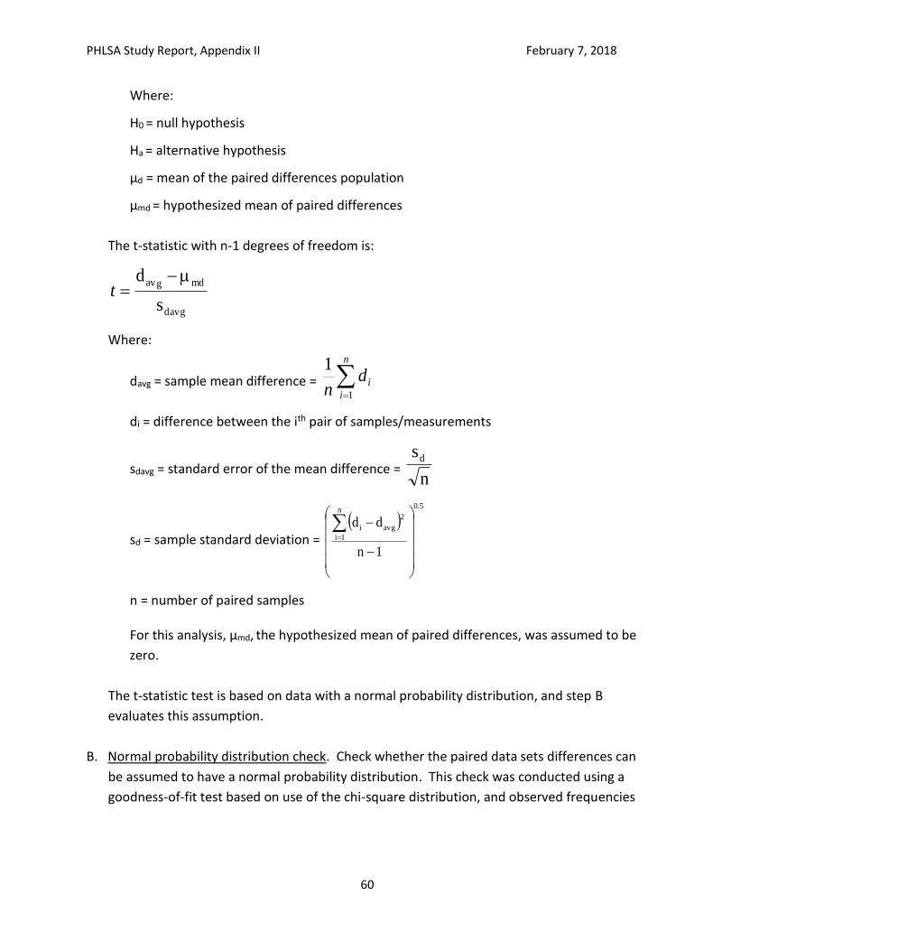
PHLSA Study Report, Appendix II February 7, 2018
60
Where:
H0 = null hypothesis
Ha = alternative hypothesis
µd = mean of the paired differences population
µmd = hypothesized mean of paired differences
The t-statistic with n-1 degrees of freedom is:
davg
mdgav
s
d t
Where:
davg = sample mean difference =
n
i
idn 1
1
di = difference between the ith pair of samples/measurements
sdavg = standard error of the mean difference = n
sd
sd = sample standard deviation =
5.0n
1i
2
avgi
1n
dd
n = number of paired samples
For this analysis, µmd, the hypothesized mean of paired differences, was assumed to be
zero.
The t-statistic test is based on data with a normal probability distribution, and step B
evaluates this assumption.
B. Normal probability distribution check. Check whether the paired data sets differences can
be assumed to have a normal probability distribution. This check was conducted using a
goodness-of-fit test based on use of the chi-square distribution, and observed frequencies
PHLSA Study Report, Appendix II February 7, 2018
61
for sample data categories are compared to the frequencies that would be expected for a
population with a normal distribution. Anderson et al2 summarize the procedure as follows:
I. State the null and alternative hypotheses:
H0: The population has a normal probability distribution
Ha: The population does not have a normal probability distribution
II. Select a random sample and
a. Compute the sample mean and sample standard deviation
b. Define intervals of values so that the expected frequency is at least five for
each interval. Using equal probability intervals is a good approach.
c. Record the observed frequency of data values fi in each interval defined.
III. Compute the expected number of occurrences ei for each interval of values defined
in II.b. Multiply the sample size by the probability of a normal random variable being in
the interval.
IV. Compute the value of the test statistic
k
i i
ii
e
ef
1
2
2
where k is the number of intervals determined in II.b.
V. Rejection rule:
Using test statistic: Reject H0 if χ2 > χα2
Using p value: Reject H0 if p-value < α
Where α is the level of significance and there are k-3 degrees of freedom.
C. Outliers check. Check for data outliers using the Dixon’s Q-test and Grubbs test for outliers.
Consider data an outlier if identified as an outlier by both tests.
Grubb’s test for outliers (one sided test)
Grubb’s test identifies a single outlier, and after that outlier is removed from the data
set additional outliers can be detected. The general procedure for the Grubb’s test is:
2 Anderson, Sweeney, & Williams, "Statistics for Business and Economics, 8th Edition". South-Western/Thomson Learning, 2002.
PHLSA Study Report, Appendix II February 7, 2018
62
I. Organize sample data from smallest number to largest number.
II. State the null and alternative hypotheses:
H0: There are no outliers in the data set
Ha: There is at least one outlier in the data set
III. Calculate the Grubb’s test statistic
s
XXor
s
XXG
avgmaxminavg
Where:
s = sample standard deviation
Xmin = minimum value
Xmax = maximum value
Xavg = sample mean
IV. Reject H0 if G > Gcritical at significance level α
Dixon’s Q-test
Dixons Q-test identifies a single outlier. After that outlier is removed from the data set,
literature guidance varies regarding whether additional outliers can be detected. For
this outlier analysis, it was assumed that a second outlier could be identified using the
Dixon’s Q-test, but outliers were only removed from the data set if detected by both the
Grubb’s and Dixon’s tests (i.e., conservative assumptions regarding outlier removal were
used).
The general procedure for the Dixons Q-test is:
I. Organize n sample data from smallest number to largest number (x1 to xn), or largest
number smallest number (x1 to xn) with the suspected outlier the first number (i.e., at
the x1 position).
II. Calculate the test statistic (for data sets larger than 14)
12
1322
xx
xxrQ
n
Where:
n = number of elements in the data set
PHLSA Study Report, Appendix II February 7, 2018
63
III. If Q > Qcritical at significance level α, then x1 can be considered an outlier
D. Normal probability distribution check, without outliers. Check whether the paired data sets
differences without statistical outliers can be assumed to have a normal probability
distribution using the goodness-of-fit test described above in Step B.
E. WSRT test. Use the Wilconxan Sign-Rank Test (WSRT) to test the null hypothesis that two
populations are identical. The WSRT can be used when the population cannot be assumed
to have a normal distribution. The general procedure is as follows:3
I. State the null and alternative hypotheses:
H0: the difference between paired samples or measurements follows a
symmetric distribution around zero
Ha: the difference between paired samples or measurements does not follow a
symmetric distribution around zero (i.e., the two populations are not identical)
II. For each sample or measurement pair (x1,i and x2,i), calculate |x2,i – x1,i| and the sign
(i.e., + or -) of (x2,i – x1,i), where i = 1 to N and N = number of sample pairs.
III. Exclude pairs with |x2,i – x1,i|= 0 and calculate Nr, where Nr = N – number of pairs
with |x2,i – x1,i|= 0
IV. Order the Nr pairs from smallest to largest |x2,i – x1,i|
V. Rank the pairs from smallest to largest with the smallest |x2,i – x1,i| with a rank of 1.
Ri denotes the rank.
VI. Calculate the test statistic W
i
Nr
i
i,i, R*xXsignW1
12
VII. Under the null hypothesis, W follows a specific distribution that has an expected
value of 0 and a variance of
6
121 rrr NNN
VIII. As Nr increases, the sampling distribution of W converges to a normal distribution
and for Nr > 10, a z-score can be calculated as
3 https://en.wikipedia.org/wiki/Wilcoxon_signed-rank_test
PHLSA Study Report, Appendix II February 7, 2018
64
W
Wz
, where σW = SQRT(variance)
IX. Reject H0 if |z| > zcritical
F. Paired data comparisons t-statistic test considering measurement uncertainty. Conduct a
paired data comparisons test to determine whether the difference between CP and CV
results were significantly greater than the measured or calculated value uncertainty.
This test used a single-tailed paired data comparisons test, and the hypothesis is:
H0: µd < µmd versus Ha: µd > µmd
Where:
µd = mean of the paired differences population
µmd = hypothesized mean of paired differences, and assumed to be the analytical
uncertainty/ reproducibility
In sum, this analysis evaluated whether the CP/CV differences were greater than the
analytical uncertainty at a given statistical significance.
G. Compile additional statistical data and summarize and discuss the results. Additional data
includes percent of paired CP/CV samples for which the CP parameter is > the CV
parameter, and the ratio of davg and (CP value + CV value)/2 (i.e., calculate davg as a percent
of the average measured value).
5.2.1.1 Initial paired data comparisons t-statistic test
Table 5-7 lists CP cylinder / CV cylinder paired pressurized condensate samples data for the GPA
2103 analyses, and calculates a t-statistic to test the null hypothesis that the mean of the paired
differences population (i.e., davg) equals 0. The data includes, by column:
Column Data
A Measured or calculated compound or parameter. These include condensate
compounds and sample bubble point pressure and FGOR calculated by PSM/EOS
B Engineering units for the compound or parameter.
C Count – number of paired samples (42)
D Average CP – average value for all the CP cylinder samples
E Average CV – average value for all the CV cylinder samples
F davg = average difference for the 42 paired samples
PHLSA Study Report, Appendix II February 7, 2018
65
G davg divided by the average of Average CP and Average CV, expressed as a
percentage. Yellow highlighted values are greater than 2%
H Standard deviation of the paired CP/CV samples differences (di values)
I Standard error of the mean difference
J t-statistic for the compound or parameter. Red high-lighted t-statistics are
greater than the critical t-statistic
K Critical t-statistic, n-1 degrees of freedom, 95% CI, 2-tailed.
This initial analysis suggests there may be statistically significant differences between CP and CV
samples for CO2, methane, ethane, propane, heptanes, octanes, 2,2,4 trimethylpentane,
PSM/EOS bubble point pressure, and PSM/EOS FGOR. 2,2,4 trimethyl pentane concentrations
are negligible and further analysis focused on the remaining compounds, with methane data
shown in the following subsections as an example.
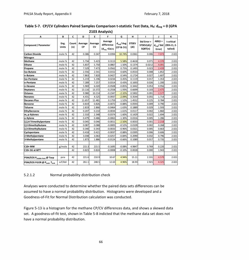
PHLSA Study Report, Appendix II February 7, 2018
66
Table 5-7. CP/CV Cylinders Paired Samples Comparison t-statistic Test Data, H0: davg = 0 (GPA
2103 Analysis)
5.2.1.2 Normal probability distribution check
Analyses were conducted to determine whether the paired data sets differences can be
assumed to have a normal probability distribution. Histograms were developed and a
Goodness-of-Fit for Normal Distribution calculation was conducted.
Figure 5-13 is a histogram for the methane CP/CV differences data, and shows a skewed data
set. A goodness-of-fit test, shown in Table 5-8 indicted that the methane data set does not
have a normal probability distribution.
A B C D E F G H I J K
Compound / ParameterEng.
Units
Count
(n)
Average
CP
Average
CV
Average
difference
(davg =Σdi/n)
davg/ Avg
(CP & CV)
STDEV
(di)
Std Error =
STDEV(di)/
SQRT(n)
ABS(t =
davg/ Std
Error)
t-critical
(95% CI, 2-
tailed)
Carbon Dioxide mole % 42 0.386 0.347 0.0394 10.74% 0.0361 0.006 7.073 2.021
Nitrogen
Methane mole % 42 5.734 5.423 0.3113 5.58% 0.4618 0.071 4.370 2.021
Ethane mole % 42 5.837 5.750 0.0867 1.50% 0.1374 0.0212 4.091 2.021
Propane mole % 42 7.529 7.473 0.0562 0.75% 0.1493 0.023 2.439 2.021
Iso-Butane mole % 42 2.556 2.541 0.0152 0.60% 0.0533 0.008 1.852 2.021
n-Butane mole % 42 7.863 7.820 0.0427 0.54% 0.1724 0.027 1.607 2.021
Iso-Pentane mole % 42 5.219 5.196 0.0234 0.45% 0.1119 0.017 1.353 2.021
n-Pentane mole % 42 7.289 7.257 0.0314 0.43% 0.1693 0.026 1.200 2.021
n-Hexane mole % 42 5.969 6.020 -0.0508 -0.85% 0.3442 0.053 0.956 2.021
Heptanes mole % 42 13.116 13.372 -0.2558 -1.93% 0.6699 0.103 2.475 2.021
Octanes mole % 42 9.980 10.214 -0.2347 -2.32% 0.5902 0.091 2.577 2.021
Nonanes mole % 42 4.431 4.525 -0.0937 -2.09% 0.3544 0.055 1.714 2.021
Decanes Plus mole % 42 11.657 11.481 0.1759 1.52% 1.4552 0.225 0.784 2.021
Benzene mole % 42 0.819 0.826 -0.0072 -0.88% 0.0593 0.009 0.790 2.021
Toluene mole % 42 2.819 2.866 -0.0464 -1.63% 0.1889 0.029 1.593 2.021
Ethylbenzene mole % 42 0.207 0.210 -0.0034 -1.61% 0.0117 0.002 1.860 2.021
m, p-Xylenes mole % 42 2.310 2.348 -0.0374 -1.60% 0.1429 0.022 1.694 2.021
o-Xylene mole % 42 0.479 0.486 -0.0063 -1.30% 0.0316 0.005 1.286 2.021
2,2,4-Trimethylpentane mole % 42 0.045 0.046 -0.0011 -2.50% 0.0033 0.001 2.218 2.021
2,2-Dimethylbutane mole % 42 0.087 0.088 -0.0005 -0.52% 0.0109 0.002 0.268 2.021
2,3-Dimethylbutane mole % 42 0.340 0.343 -0.0033 -0.96% 0.0321 0.005 0.663 2.021
Cyclopentane mole % 42 0.418 0.421 -0.0037 -0.88% 0.0395 0.006 0.606 2.021
2-Methylpentane mole % 42 3.038 3.063 -0.0257 -0.84% 0.2090 0.032 0.796 2.021
3-Methylpentane mole % 42 1.873 1.886 -0.0124 -0.66% 0.1089 0.017 0.735 2.021
C10+ MW g/mole 42 215.3 215.5 -0.1695 -0.08% 4.9847 0.769 0.220 2.021
C10+ SG at 60°F 42 0.823 0.824 -0.0008 -0.10% 0.0028 0.000 1.943 2.021
PSM/EOS PBubble Point @ Tsep psia 42 221.6 210.9 10.67 4.94% 15.11 2.331 4.579 2.021
PSM/EOS FGOR @ Ptank, Ttank scf/bbl 42 261.1 248.5 12.63 4.96% 18.93 2.921 4.325 2.021
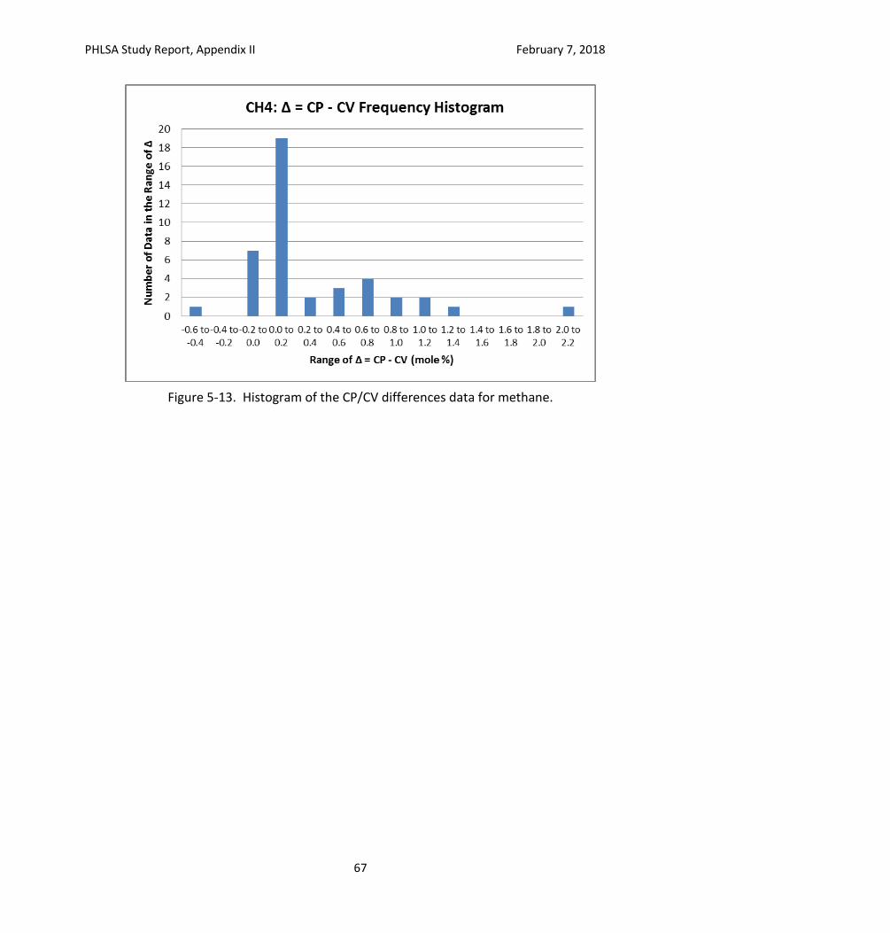
PHLSA Study Report, Appendix II February 7, 2018
67
Figure 5-13. Histogram of the CP/CV differences data for methane.
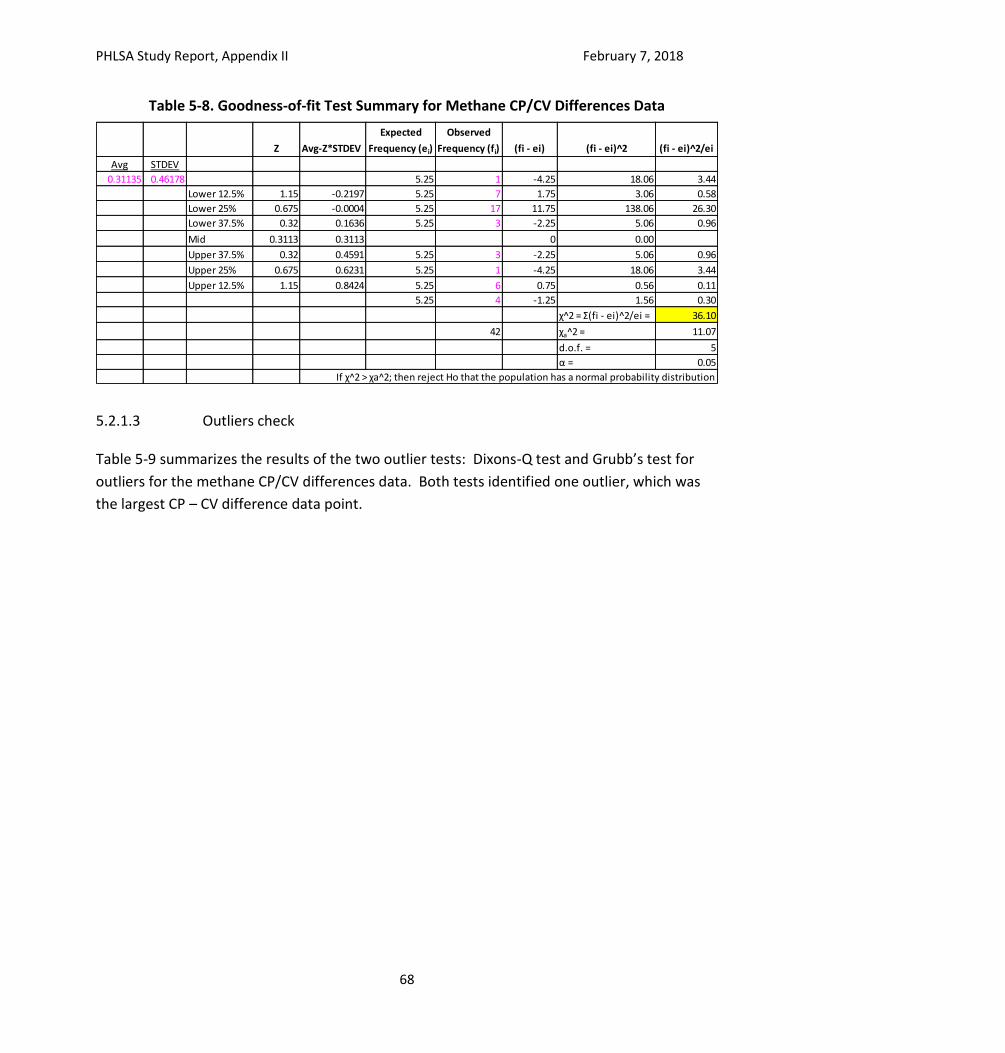
PHLSA Study Report, Appendix II February 7, 2018
68
Table 5-8. Goodness-of-fit Test Summary for Methane CP/CV Differences Data
5.2.1.3 Outliers check
Table 5-9 summarizes the results of the two outlier tests: Dixons-Q test and Grubb’s test for
outliers for the methane CP/CV differences data. Both tests identified one outlier, which was
the largest CP – CV difference data point.
Z Avg-Z*STDEV
Expected
Frequency (ei)
Observed
Frequency (fi) (fi - ei) (fi - ei)^2 (fi - ei)^2/ei
Avg STDEV
0.31135 0.46178 5.25 1 -4.25 18.06 3.44
Lower 12.5% 1.15 -0.2197 5.25 7 1.75 3.06 0.58
Lower 25% 0.675 -0.0004 5.25 17 11.75 138.06 26.30
Lower 37.5% 0.32 0.1636 5.25 3 -2.25 5.06 0.96
Mid 0.3113 0.3113 0 0.00
Upper 37.5% 0.32 0.4591 5.25 3 -2.25 5.06 0.96
Upper 25% 0.675 0.6231 5.25 1 -4.25 18.06 3.44
Upper 12.5% 1.15 0.8424 5.25 6 0.75 0.56 0.11
5.25 4 -1.25 1.56 0.30
χ^2 = Σ(fi - ei)^2/ei = 36.10
42 χa^2 = 11.07
d.o.f. = 5
α = 0.05
If χ^2 > χa^2; then reject Ho that the population has a normal probability distribution
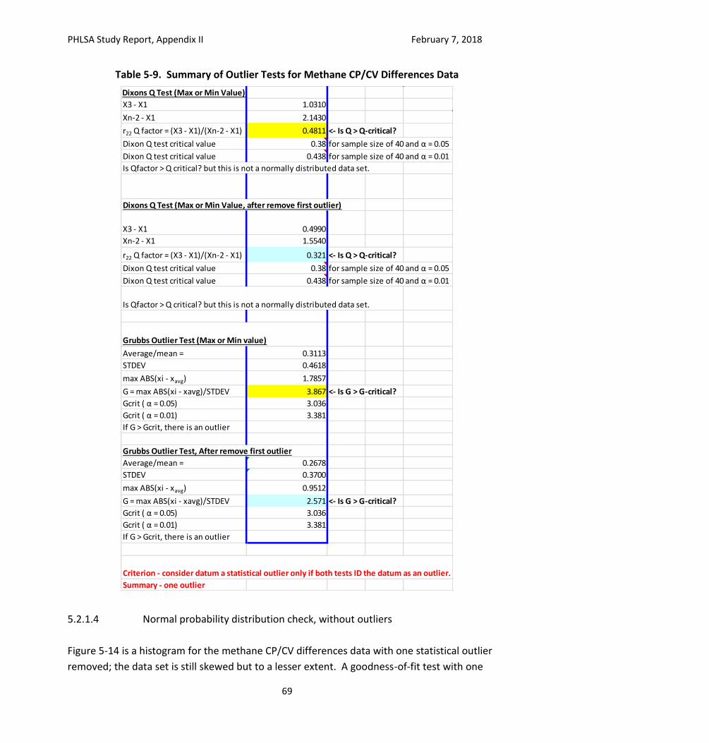
PHLSA Study Report, Appendix II February 7, 2018
69
Table 5-9. Summary of Outlier Tests for Methane CP/CV Differences Data
5.2.1.4 Normal probability distribution check, without outliers
Figure 5-14 is a histogram for the methane CP/CV differences data with one statistical outlier
removed; the data set is still skewed but to a lesser extent. A goodness-of-fit test with one
Dixons Q Test (Max or Min Value)
X3 - X1 1.0310
Xn-2 - X1 2.1430
r22 Q factor = (X3 - X1)/(Xn-2 - X1) 0.4811 <- Is Q > Q-critical?
Dixon Q test critical value 0.38 for sample size of 40 and α = 0.05
Dixon Q test critical value 0.438 for sample size of 40 and α = 0.01
Is Qfactor > Q critical? but this is not a normally distributed data set.
Dixons Q Test (Max or Min Value, after remove first outlier)
X3 - X1 0.4990
Xn-2 - X1 1.5540
r22 Q factor = (X3 - X1)/(Xn-2 - X1) 0.321 <- Is Q > Q-critical?
Dixon Q test critical value 0.38 for sample size of 40 and α = 0.05
Dixon Q test critical value 0.438 for sample size of 40 and α = 0.01
Is Qfactor > Q critical? but this is not a normally distributed data set.
Grubbs Outlier Test (Max or Min value)
Average/mean = 0.3113
STDEV 0.4618
max ABS(xi - xavg) 1.7857
G = max ABS(xi - xavg)/STDEV 3.867 <- Is G > G-critical?
Gcrit ( α = 0.05) 3.036
Gcrit ( α = 0.01) 3.381
If G > Gcrit, there is an outlier
Grubbs Outlier Test, After remove first outlier
Average/mean = 0.2678
STDEV 0.3700
max ABS(xi - xavg) 0.9512
G = max ABS(xi - xavg)/STDEV 2.571 <- Is G > G-critical?
Gcrit ( α = 0.05) 3.036
Gcrit ( α = 0.01) 3.381
If G > Gcrit, there is an outlier
Summary - one outlier
Criterion - consider datum a statistical outlier only if both tests ID the datum as an outlier.
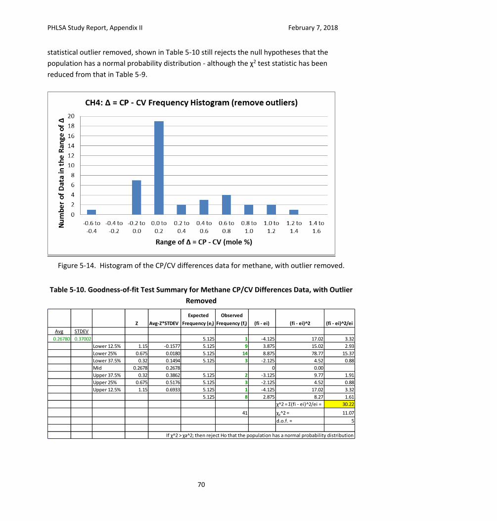
PHLSA Study Report, Appendix II February 7, 2018
70
statistical outlier removed, shown in Table 5-10 still rejects the null hypotheses that the
population has a normal probability distribution - although the χ2 test statistic has been
reduced from that in Table 5-9.
Figure 5-14. Histogram of the CP/CV differences data for methane, with outlier removed.
Table 5-10. Goodness-of-fit Test Summary for Methane CP/CV Differences Data, with Outlier
Removed
Z Avg-Z*STDEV
Expected
Frequency (ei)
Observed
Frequency (fi) (fi - ei) (fi - ei)^2 (fi - ei)^2/ei
Avg STDEV
0.26780 0.37002 5.125 1 -4.125 17.02 3.32
Lower 12.5% 1.15 -0.1577 5.125 9 3.875 15.02 2.93
Lower 25% 0.675 0.0180 5.125 14 8.875 78.77 15.37
Lower 37.5% 0.32 0.1494 5.125 3 -2.125 4.52 0.88
Mid 0.2678 0.2678 0 0.00
Upper 37.5% 0.32 0.3862 5.125 2 -3.125 9.77 1.91
Upper 25% 0.675 0.5176 5.125 3 -2.125 4.52 0.88
Upper 12.5% 1.15 0.6933 5.125 1 -4.125 17.02 3.32
5.125 8 2.875 8.27 1.61
χ^2 = Σ(fi - ei)^2/ei = 30.22
41 χa^2 = 11.07
d.o.f. = 5
If χ^2 > χa^2; then reject Ho that the population has a normal probability distribution
PHLSA Study Report, Appendix II February 7, 2018
71
5.2.1.5 Wilconxan Sign-Rank Test (WSRT)
Table 5-11 shows the WSRT analysis of the methane CP/CV differences data. The test statistic is
greater than zcritical for the data sets with and without the outliers; thus the null hypothesis that
the two populations are identical is rejected and it is concluded, that for samples collected for
this project, that methane concentrations measured in pressurized condensate collected with a
CP cylinder differ from methane concentrations measured in pressurized condensate collected
with a CV cylinder.
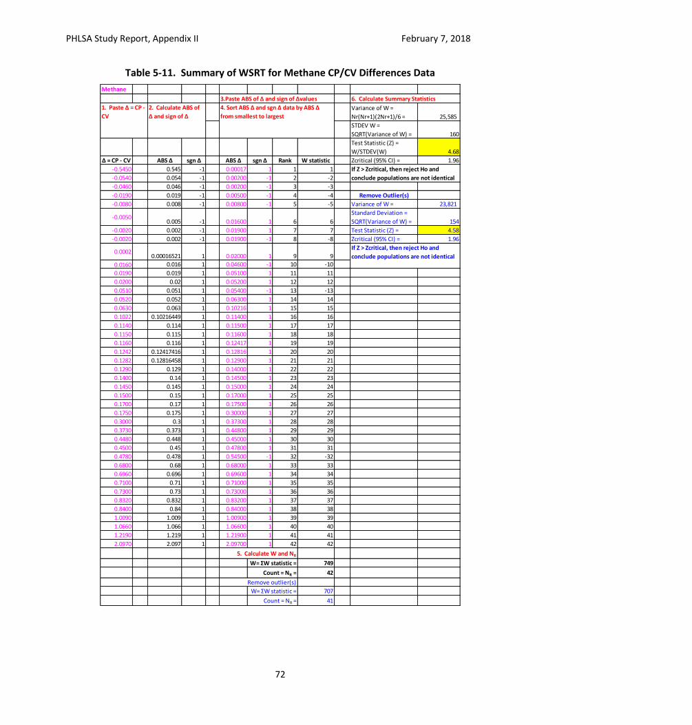
PHLSA Study Report, Appendix II February 7, 2018
72
Table 5-11. Summary of WSRT for Methane CP/CV Differences Data
Methane
3.Paste ABS of Δ and sign of Δvalues 6. Calculate Summary Statistics
Variance of W =
Nr(Nr+1)(2Nr+1)/6 = 25,585
STDEV W =
SQRT(Variance of W) = 160
Test Statistic (Z) =
W/STDEV(W) 4.68
Δ = CP - CV ABS Δ sgn Δ ABS Δ sgn Δ Rank W statistic Zcritical (95% CI) = 1.96
-0.5450 0.545 -1 0.00017 1 1 1
-0.0540 0.054 -1 0.00200 -1 2 -2
-0.0460 0.046 -1 0.00200 -1 3 -3
-0.0190 0.019 -1 0.00500 -1 4 -4 Remove Outlier(s)
-0.0080 0.008 -1 0.00800 -1 5 -5 Variance of W = 23,821
-0.00500.005 -1 0.01600 1 6 6
Standard Deviation =
SQRT(Variance of W) = 154
-0.0020 0.002 -1 0.01900 1 7 7 Test Statistic (Z) = 4.58
-0.0020 0.002 -1 0.01900 -1 8 -8 Zcritical (95% CI) = 1.96
0.00020.00016521 1 0.02000 1 9 9
0.0160 0.016 1 0.04600 -1 10 -10
0.0190 0.019 1 0.05100 1 11 11
0.0200 0.02 1 0.05200 1 12 12
0.0510 0.051 1 0.05400 -1 13 -13
0.0520 0.052 1 0.06300 1 14 14
0.0630 0.063 1 0.10216 1 15 15
0.1022 0.10216449 1 0.11400 1 16 16
0.1140 0.114 1 0.11500 1 17 17
0.1150 0.115 1 0.11600 1 18 18
0.1160 0.116 1 0.12417 1 19 19
0.1242 0.12417416 1 0.12816 1 20 20
0.1282 0.12816458 1 0.12900 1 21 21
0.1290 0.129 1 0.14000 1 22 22
0.1400 0.14 1 0.14500 1 23 23
0.1450 0.145 1 0.15000 1 24 24
0.1500 0.15 1 0.17000 1 25 25
0.1700 0.17 1 0.17500 1 26 26
0.1750 0.175 1 0.30000 1 27 27
0.3000 0.3 1 0.37300 1 28 28
0.3730 0.373 1 0.44800 1 29 29
0.4480 0.448 1 0.45000 1 30 30
0.4500 0.45 1 0.47800 1 31 31
0.4780 0.478 1 0.54500 -1 32 -32
0.6800 0.68 1 0.68000 1 33 33
0.6960 0.696 1 0.69600 1 34 34
0.7100 0.71 1 0.71000 1 35 35
0.7300 0.73 1 0.73000 1 36 36
0.8320 0.832 1 0.83200 1 37 37
0.8400 0.84 1 0.84000 1 38 38
1.0090 1.009 1 1.00900 1 39 39
1.0660 1.066 1 1.06600 1 40 40
1.2190 1.219 1 1.21900 1 41 41
2.0970 2.097 1 2.09700 1 42 42
5. Calculate W and NR
W= ΣW statistic = 749
Count = NR = 42
Remove outlier(s)
W= ΣW statistic = 707
Count = NR = 41
4. Sort ABS Δ and sgn Δ data by ABS Δ
from smallest to largest
2. Calculate ABS of
Δ and sign of Δ
1. Paste Δ = CP -
CV
If Z > Zcritical, then reject Ho and
conclude populations are not identical
If Z > Zcritical, then reject Ho and
conclude populations are not identical
PHLSA Study Report, Appendix II February 7, 2018
73
5.2.1.6 Paired data comparisons t-statistic test considering measurement uncertainty.
Table 5-12 lists CP cylinder / CV cylinder paired pressurized condensate samples data for the
GPA 2103 analyses, and calculates a t-statistic to test the null hypothesis that the mean of the
paired differences population (i.e., davg) is less than or equal to the analytical method
uncertainty for the contract lab. The data includes, by column:
Column Data
A Measured compound.
B Engineering units for the compound.
C Count – number of paired samples (42)
D Average CP – average value for all the CP cylinder samples
E Average CV – average value for all the CV cylinder samples
F davg = average difference for the 42 paired samples
G Standard deviation of the paired CP/CV samples differences (di values)
H Standard error of the mean difference
I Analytical method uncertainty expressed as a percentage of the measured value
J Analytical method uncertainty expressed in engineering unit
K t-statistic for the compound or parameter. Red high-lighted t-statistics are
greater than the critical t-statistic for a 99% CI, and blue high-lighted t-statistics
are greater than the critical t-statistic for a 95% CI.
L Critical t-statistic, n-1 degrees of freedom, 99% CI, 1-tailed.
M Critical t-statistic, n-1 degrees of freedom, 95% CI, 1-tailed.
This analysis suggests that the differences between CP and CV samples for CO2 and methane
are statistically significant, even when the analytical uncertainty is considered. The t-statistics
for CO2 and methane indicate that the null hypothesis is rejected at 99% probability, providing
additional support for these conclusions considering that the population of differences for
these parameters may not be normally distributed.
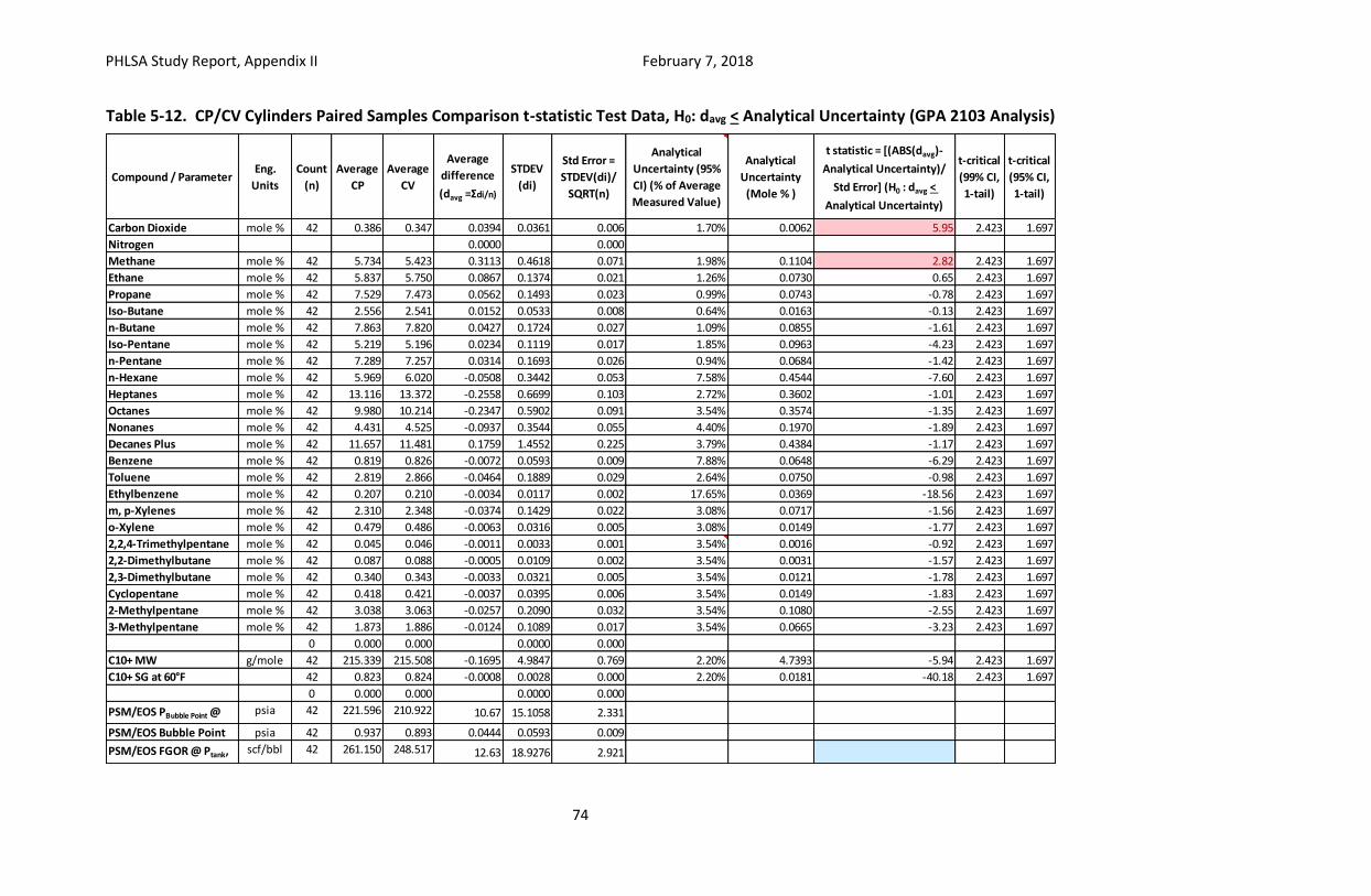
PHLSA Study Report, Appendix II February 7, 2018
74
Table 5-12. CP/CV Cylinders Paired Samples Comparison t-statistic Test Data, H0: davg < Analytical Uncertainty (GPA 2103 Analysis)
Compound / ParameterEng.
Units
Count
(n)
Average
CP
Average
CV
Average
difference
(davg =Σdi/n)
STDEV
(di)
Std Error =
STDEV(di)/
SQRT(n)
Analytical
Uncertainty (95%
CI) (% of Average
Measured Value)
Analytical
Uncertainty
(Mole % )
t statistic = [(ABS(davg)-
Analytical Uncertainty)/
Std Error] (H0 : davg <
Analytical Uncertainty)
t-critical
(99% CI,
1-tail)
t-critical
(95% CI,
1-tail)
Carbon Dioxide mole % 42 0.386 0.347 0.0394 0.0361 0.006 1.70% 0.0062 5.95 2.423 1.697
Nitrogen 0.0000 0.000
Methane mole % 42 5.734 5.423 0.3113 0.4618 0.071 1.98% 0.1104 2.82 2.423 1.697
Ethane mole % 42 5.837 5.750 0.0867 0.1374 0.021 1.26% 0.0730 0.65 2.423 1.697
Propane mole % 42 7.529 7.473 0.0562 0.1493 0.023 0.99% 0.0743 -0.78 2.423 1.697
Iso-Butane mole % 42 2.556 2.541 0.0152 0.0533 0.008 0.64% 0.0163 -0.13 2.423 1.697
n-Butane mole % 42 7.863 7.820 0.0427 0.1724 0.027 1.09% 0.0855 -1.61 2.423 1.697
Iso-Pentane mole % 42 5.219 5.196 0.0234 0.1119 0.017 1.85% 0.0963 -4.23 2.423 1.697
n-Pentane mole % 42 7.289 7.257 0.0314 0.1693 0.026 0.94% 0.0684 -1.42 2.423 1.697
n-Hexane mole % 42 5.969 6.020 -0.0508 0.3442 0.053 7.58% 0.4544 -7.60 2.423 1.697
Heptanes mole % 42 13.116 13.372 -0.2558 0.6699 0.103 2.72% 0.3602 -1.01 2.423 1.697
Octanes mole % 42 9.980 10.214 -0.2347 0.5902 0.091 3.54% 0.3574 -1.35 2.423 1.697
Nonanes mole % 42 4.431 4.525 -0.0937 0.3544 0.055 4.40% 0.1970 -1.89 2.423 1.697
Decanes Plus mole % 42 11.657 11.481 0.1759 1.4552 0.225 3.79% 0.4384 -1.17 2.423 1.697
Benzene mole % 42 0.819 0.826 -0.0072 0.0593 0.009 7.88% 0.0648 -6.29 2.423 1.697
Toluene mole % 42 2.819 2.866 -0.0464 0.1889 0.029 2.64% 0.0750 -0.98 2.423 1.697
Ethylbenzene mole % 42 0.207 0.210 -0.0034 0.0117 0.002 17.65% 0.0369 -18.56 2.423 1.697
m, p-Xylenes mole % 42 2.310 2.348 -0.0374 0.1429 0.022 3.08% 0.0717 -1.56 2.423 1.697
o-Xylene mole % 42 0.479 0.486 -0.0063 0.0316 0.005 3.08% 0.0149 -1.77 2.423 1.697
2,2,4-Trimethylpentane mole % 42 0.045 0.046 -0.0011 0.0033 0.001 3.54% 0.0016 -0.92 2.423 1.697
2,2-Dimethylbutane mole % 42 0.087 0.088 -0.0005 0.0109 0.002 3.54% 0.0031 -1.57 2.423 1.697
2,3-Dimethylbutane mole % 42 0.340 0.343 -0.0033 0.0321 0.005 3.54% 0.0121 -1.78 2.423 1.697
Cyclopentane mole % 42 0.418 0.421 -0.0037 0.0395 0.006 3.54% 0.0149 -1.83 2.423 1.697
2-Methylpentane mole % 42 3.038 3.063 -0.0257 0.2090 0.032 3.54% 0.1080 -2.55 2.423 1.697
3-Methylpentane mole % 42 1.873 1.886 -0.0124 0.1089 0.017 3.54% 0.0665 -3.23 2.423 1.697
0 0.000 0.000 0.0000 0.000
C10+ MW g/mole 42 215.339 215.508 -0.1695 4.9847 0.769 2.20% 4.7393 -5.94 2.423 1.697
C10+ SG at 60°F 42 0.823 0.824 -0.0008 0.0028 0.000 2.20% 0.0181 -40.18 2.423 1.697
0 0.000 0.000 0.0000 0.000
PSM/EOS PBubble Point @
Tsep
psia 42 221.596 210.922 10.67 15.1058 2.331
PSM/EOS Bubble Point psia 42 0.937 0.893 0.0444 0.0593 0.009
PSM/EOS FGOR @ Ptank,
Ttank
scf/bbl 42 261.150 248.517 12.63 18.9276 2.921
PHLSA Study Report, Appendix II February 7, 2018
75
5.2.1.7 Statistical data summary
Table 5-13 summarizes statistics for the CP/CV cylinders paired samples differences data. The table
includes data for the compounds and parameters identified in Table 5-7 as having a statistically significant
difference between CP and CV samples. In addition to the paired sample t-statistic and WRST results
presented previously, this table includes the percent of paired CP/CV samples for which the CP parameter is
> the CV parameter, and the ratio of davg and (CP value + CV value)/2 (i.e., calculate davg as a percent of the
average measured value).
For 100% of the paired CP/CV cylinder samples, the CP cylinder had a higher concentration of carbon
dioxide, and on average this difference was about 10.7% of the CO2 concentration. These data, and the
results of the paired data comparisons t-statistic test considering measurement uncertainty, indicate
that the difference between the CP cylinder and CV cylinder measurements of CO2 in pressurized
condensate is statistical significant.
In 81% of the paired CP/CV cylinder samples, the CP cylinder had a higher concentration of methane, and
the overall average difference (CP – CV) was about 5.6% of the methane concentration. These data, and
the results of the paired data comparisons t-statistic test considering measurement uncertainty, indicate
that there was a statistically significant difference between the CP cylinder and CV cylinder
measurements of methane in pressurized condensate.
For both PSM/EOS bubble point pressure and PSM/EOS FGOR, over 80% of the paired CP/CV cylinder
samples had higher calculated values for the CP cylinder and the overall average difference (CP – CV) was
about 5% of the calculated value. These data, and the results of the paired data comparisons t-statistic
test, indicate that there was difference between the PSM/EOS calculated estimates of PBP and FGOR
based on the CP cylinder pressurized condensate samples and the PSM/EOS calculated estimates of PBP
and FGOR based on the CV cylinder pressurized condensate samples.
Both PBP and FGOR are strongly impacted by CO2 and methane concentrations in the pressurized
condensate; thus, these results are consistent with CP/CV results for methane and CO2.
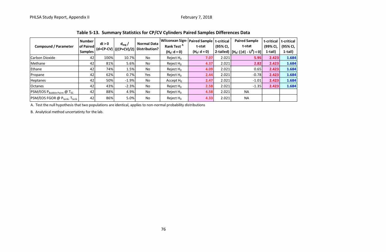
PHLSA Study Report, Appendix II February 7, 2018
76
Table 5-13. Summary Statistics for CP/CV Cylinders Paired Samples Differences Data
Compound / Parameter
Number
of Paired
Samples
di > 0
(d=CP-CV)
davg /
((CP+CV)/2)
Normal Data
Distribution?
Wilconxan Sign-
Rank Test A
(H0: d = 0)
Paired Sample
t-stat
(H0: d = 0)
t-critical
(95% CI,
2-tailed)
Paired Sample
t-stat
[H0: (|d| - UB) < 0]
t-critical
(99% CI,
1-tail)
t-critical
(95% CI,
1-tail)
Carbon Dioxide 42 100% 10.7% No Reject H0 7.07 2.021 5.95 2.423 1.684
Methane 42 81% 5.6% No Reject H0 4.37 2.021 2.82 2.423 1.684
Ethane 42 74% 1.5% No Reject H0 4.09 2.021 0.65 2.423 1.684
Propane 42 62% 0.7% Yes Reject H0 2.44 2.021 -0.78 2.423 1.684
Heptanes 42 50% -1.9% No Accept H0 2.47 2.021 -1.01 2.423 1.684
Octanes 42 43% -2.3% No Reject H0 2.58 2.021 -1.35 2.423 1.684
PSM/EOS PBubble Point @ TSC 42 88% 4.9% No Reject H0 4.58 2.021 NA
PSM/EOS FGOR @ Ptank, Ttank 42 86% 5.0% No Reject H0 4.33 2.021 NA
A. Test the null hypothesis that two populations are identical, applies to non-normal probability distributions
B. Analytical method uncertatinty for the lab.
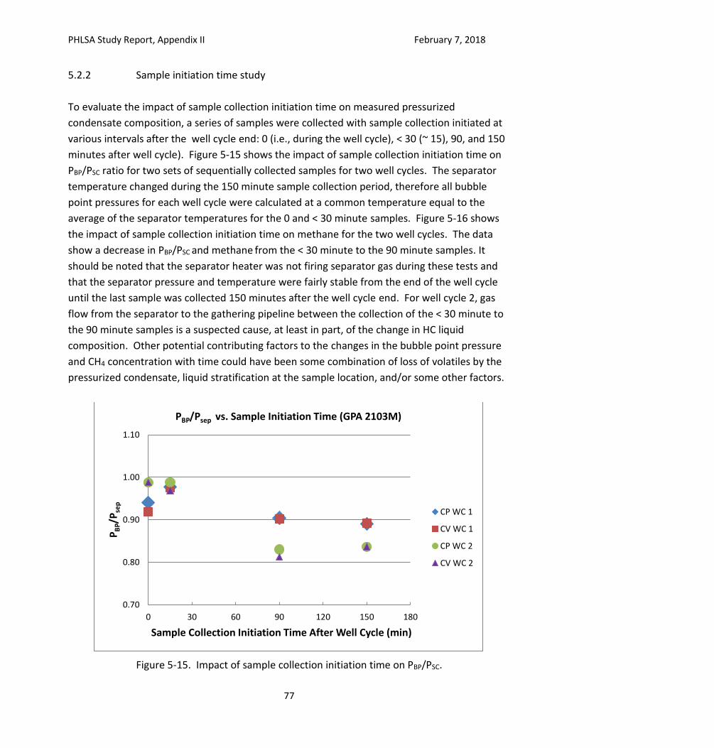
PHLSA Study Report, Appendix II February 7, 2018
77
5.2.2 Sample initiation time study
To evaluate the impact of sample collection initiation time on measured pressurized
condensate composition, a series of samples were collected with sample collection initiated at
various intervals after the well cycle end: 0 (i.e., during the well cycle), < 30 (~ 15), 90, and 150
minutes after well cycle). Figure 5-15 shows the impact of sample collection initiation time on
PBP/PSC ratio for two sets of sequentially collected samples for two well cycles. The separator
temperature changed during the 150 minute sample collection period, therefore all bubble
point pressures for each well cycle were calculated at a common temperature equal to the
average of the separator temperatures for the 0 and < 30 minute samples. Figure 5-16 shows
the impact of sample collection initiation time on methane for the two well cycles. The data
show a decrease in PBP/PSC and methane from the < 30 minute to the 90 minute samples. It
should be noted that the separator heater was not firing separator gas during these tests and
that the separator pressure and temperature were fairly stable from the end of the well cycle
until the last sample was collected 150 minutes after the well cycle end. For well cycle 2, gas
flow from the separator to the gathering pipeline between the collection of the < 30 minute to
the 90 minute samples is a suspected cause, at least in part, of the change in HC liquid
composition. Other potential contributing factors to the changes in the bubble point pressure
and CH4 concentration with time could have been some combination of loss of volatiles by the
pressurized condensate, liquid stratification at the sample location, and/or some other factors.
Figure 5-15. Impact of sample collection initiation time on PBP/PSC.
0.70
0.80
0.90
1.00
1.10
0 30 60 90 120 150 180
PB
P/P
sep
Sample Collection Initiation Time After Well Cycle (min)
PBP/Psep vs. Sample Initiation Time (GPA 2103M)
CP WC 1
CV WC 1
CP WC 2
CV WC 2
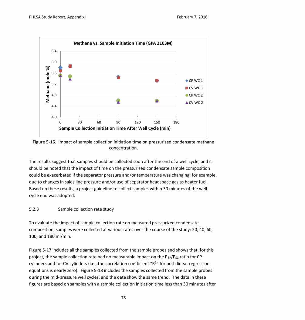
PHLSA Study Report, Appendix II February 7, 2018
78
Figure 5-16. Impact of sample collection initiation time on pressurized condensate methane
concentration.
The results suggest that samples should be collected soon after the end of a well cycle, and it
should be noted that the impact of time on the pressurized condensate sample composition
could be exacerbated if the separator pressure and/or temperature was changing; for example,
due to changes in sales line pressure and/or use of separator headspace gas as heater fuel.
Based on these results, a project guideline to collect samples within 30 minutes of the well
cycle end was adopted.
5.2.3 Sample collection rate study
To evaluate the impact of sample collection rate on measured pressurized condensate
composition, samples were collected at various rates over the course of the study: 20, 40, 60,
100, and 180 ml/min.
Figure 5-17 includes all the samples collected from the sample probes and shows that, for this
project, the sample collection rate had no measurable impact on the PBP/PSC ratio for CP
cylinders and for CV cylinders (i.e., the correlation coefficient “R2” for both linear regression
equations is nearly zero). Figure 5-18 includes the samples collected from the sample probes
during the mid-pressure well cycles, and the data show the same trend. The data in these
figures are based on samples with a sample collection initiation time less than 30 minutes after
4.0
4.4
4.8
5.2
5.6
6.0
6.4
0 30 60 90 120 150 180
Met
han
e (m
ole
%)
Sample Collection Initiation Time After Well Cycle (min)
Methane vs. Sample Initiation Time (GPA 2103M)
CP WC 1
CV WC 1
CP WC 2
CV WC 2
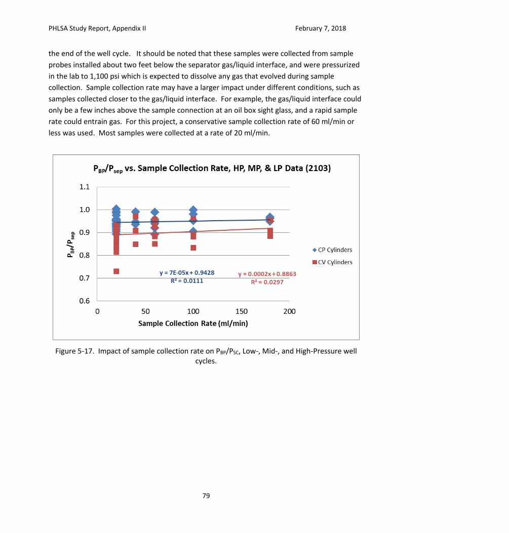
PHLSA Study Report, Appendix II February 7, 2018
79
the end of the well cycle. It should be noted that these samples were collected from sample
probes installed about two feet below the separator gas/liquid interface, and were pressurized
in the lab to 1,100 psi which is expected to dissolve any gas that evolved during sample
collection. Sample collection rate may have a larger impact under different conditions, such as
samples collected closer to the gas/liquid interface. For example, the gas/liquid interface could
only be a few inches above the sample connection at an oil box sight glass, and a rapid sample
rate could entrain gas. For this project, a conservative sample collection rate of 60 ml/min or
less was used. Most samples were collected at a rate of 20 ml/min.
Figure 5-17. Impact of sample collection rate on PBP/PSC, Low-, Mid-, and High-Pressure well cycles.
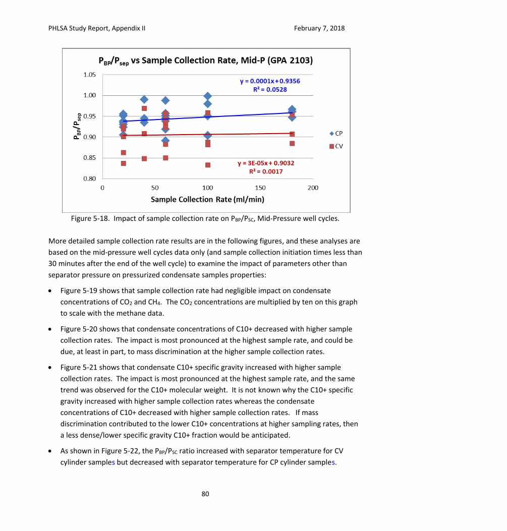
PHLSA Study Report, Appendix II February 7, 2018
80
Figure 5-18. Impact of sample collection rate on PBP/PSC, Mid-Pressure well cycles.
More detailed sample collection rate results are in the following figures, and these analyses are
based on the mid-pressure well cycles data only (and sample collection initiation times less than
30 minutes after the end of the well cycle) to examine the impact of parameters other than
separator pressure on pressurized condensate samples properties:
Figure 5-19 shows that sample collection rate had negligible impact on condensate
concentrations of CO2 and CH4. The CO2 concentrations are multiplied by ten on this graph
to scale with the methane data.
Figure 5-20 shows that condensate concentrations of C10+ decreased with higher sample
collection rates. The impact is most pronounced at the highest sample rate, and could be
due, at least in part, to mass discrimination at the higher sample collection rates.
Figure 5-21 shows that condensate C10+ specific gravity increased with higher sample
collection rates. The impact is most pronounced at the highest sample rate, and the same
trend was observed for the C10+ molecular weight. It is not known why the C10+ specific
gravity increased with higher sample collection rates whereas the condensate
concentrations of C10+ decreased with higher sample collection rates. If mass
discrimination contributed to the lower C10+ concentrations at higher sampling rates, then
a less dense/lower specific gravity C10+ fraction would be anticipated.
As shown in Figure 5-22, the PBP/PSC ratio increased with separator temperature for CV
cylinder samples but decreased with separator temperature for CP cylinder samples.
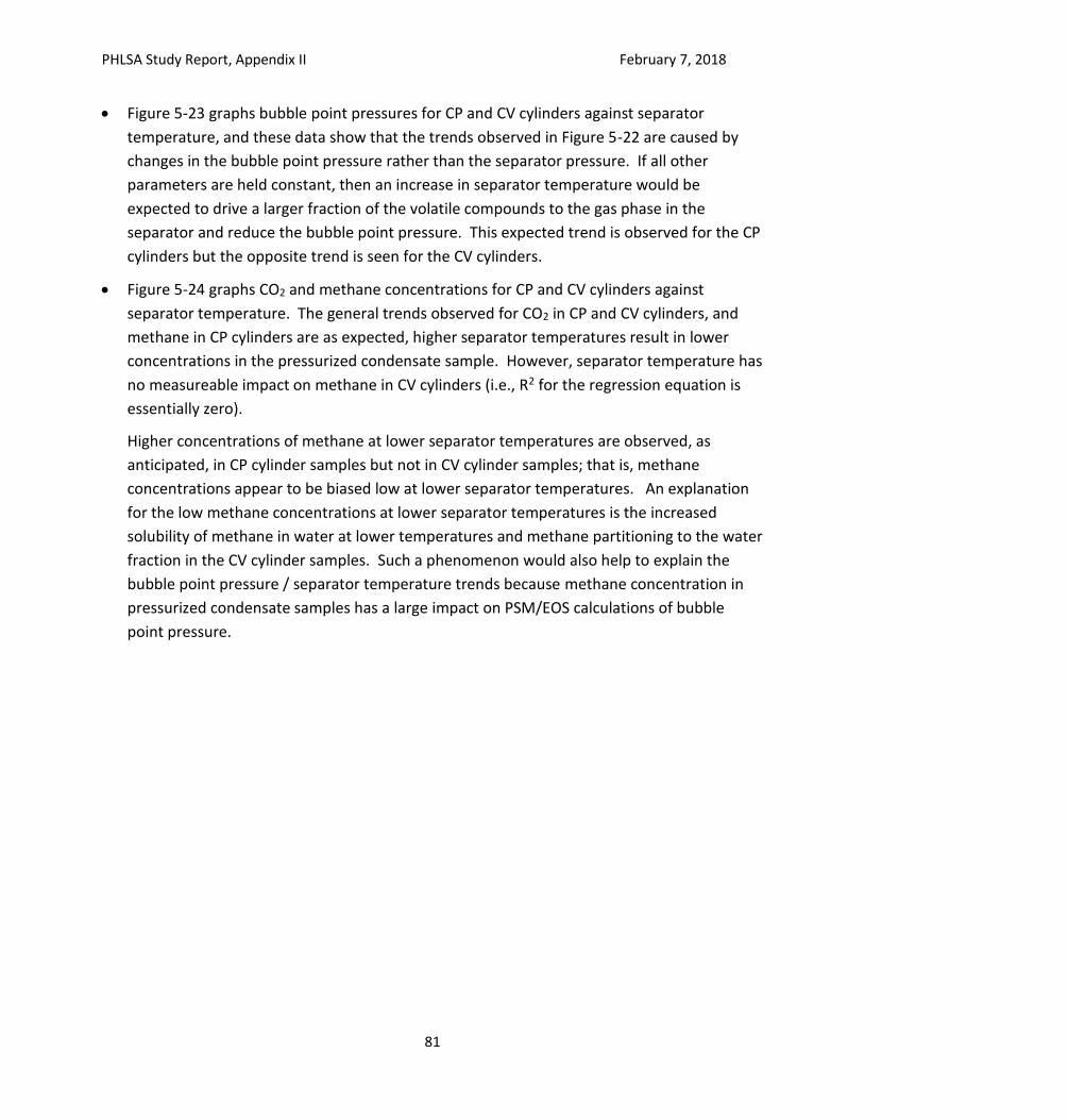
PHLSA Study Report, Appendix II February 7, 2018
81
Figure 5-23 graphs bubble point pressures for CP and CV cylinders against separator
temperature, and these data show that the trends observed in Figure 5-22 are caused by
changes in the bubble point pressure rather than the separator pressure. If all other
parameters are held constant, then an increase in separator temperature would be
expected to drive a larger fraction of the volatile compounds to the gas phase in the
separator and reduce the bubble point pressure. This expected trend is observed for the CP
cylinders but the opposite trend is seen for the CV cylinders.
Figure 5-24 graphs CO2 and methane concentrations for CP and CV cylinders against
separator temperature. The general trends observed for CO2 in CP and CV cylinders, and
methane in CP cylinders are as expected, higher separator temperatures result in lower
concentrations in the pressurized condensate sample. However, separator temperature has
no measureable impact on methane in CV cylinders (i.e., R2 for the regression equation is
essentially zero).
Higher concentrations of methane at lower separator temperatures are observed, as
anticipated, in CP cylinder samples but not in CV cylinder samples; that is, methane
concentrations appear to be biased low at lower separator temperatures. An explanation
for the low methane concentrations at lower separator temperatures is the increased
solubility of methane in water at lower temperatures and methane partitioning to the water
fraction in the CV cylinder samples. Such a phenomenon would also help to explain the
bubble point pressure / separator temperature trends because methane concentration in
pressurized condensate samples has a large impact on PSM/EOS calculations of bubble
point pressure.
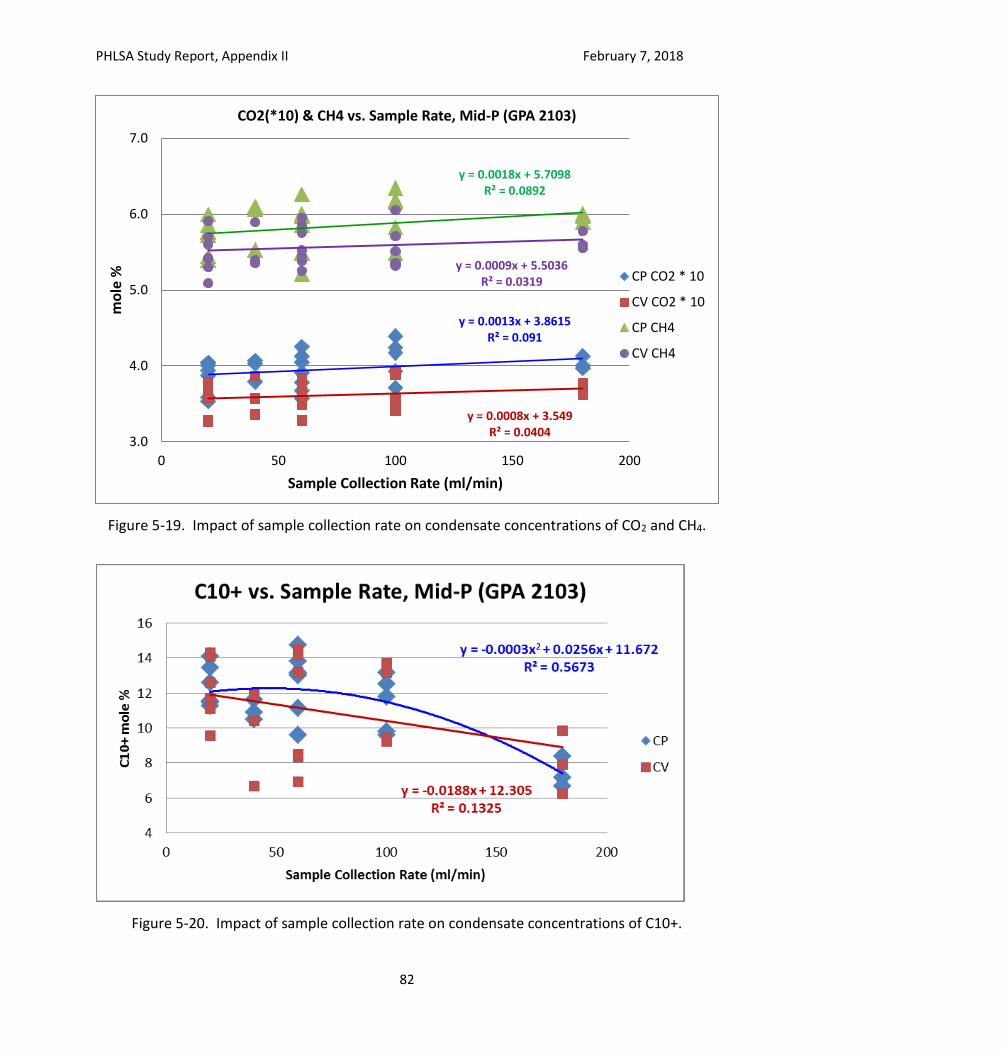
PHLSA Study Report, Appendix II February 7, 2018
82
Figure 5-19. Impact of sample collection rate on condensate concentrations of CO2 and CH4.
Figure 5-20. Impact of sample collection rate on condensate concentrations of C10+.
y = 0.0013x + 3.8615R² = 0.091
y = 0.0008x + 3.549R² = 0.0404
y = 0.0018x + 5.7098R² = 0.0892
y = 0.0009x + 5.5036R² = 0.0319
3.0
4.0
5.0
6.0
7.0
0 50 100 150 200
mo
le %
Sample Collection Rate (ml/min)
CO2(*10) & CH4 vs. Sample Rate, Mid-P (GPA 2103)
CP CO2 * 10
CV CO2 * 10
CP CH4
CV CH4
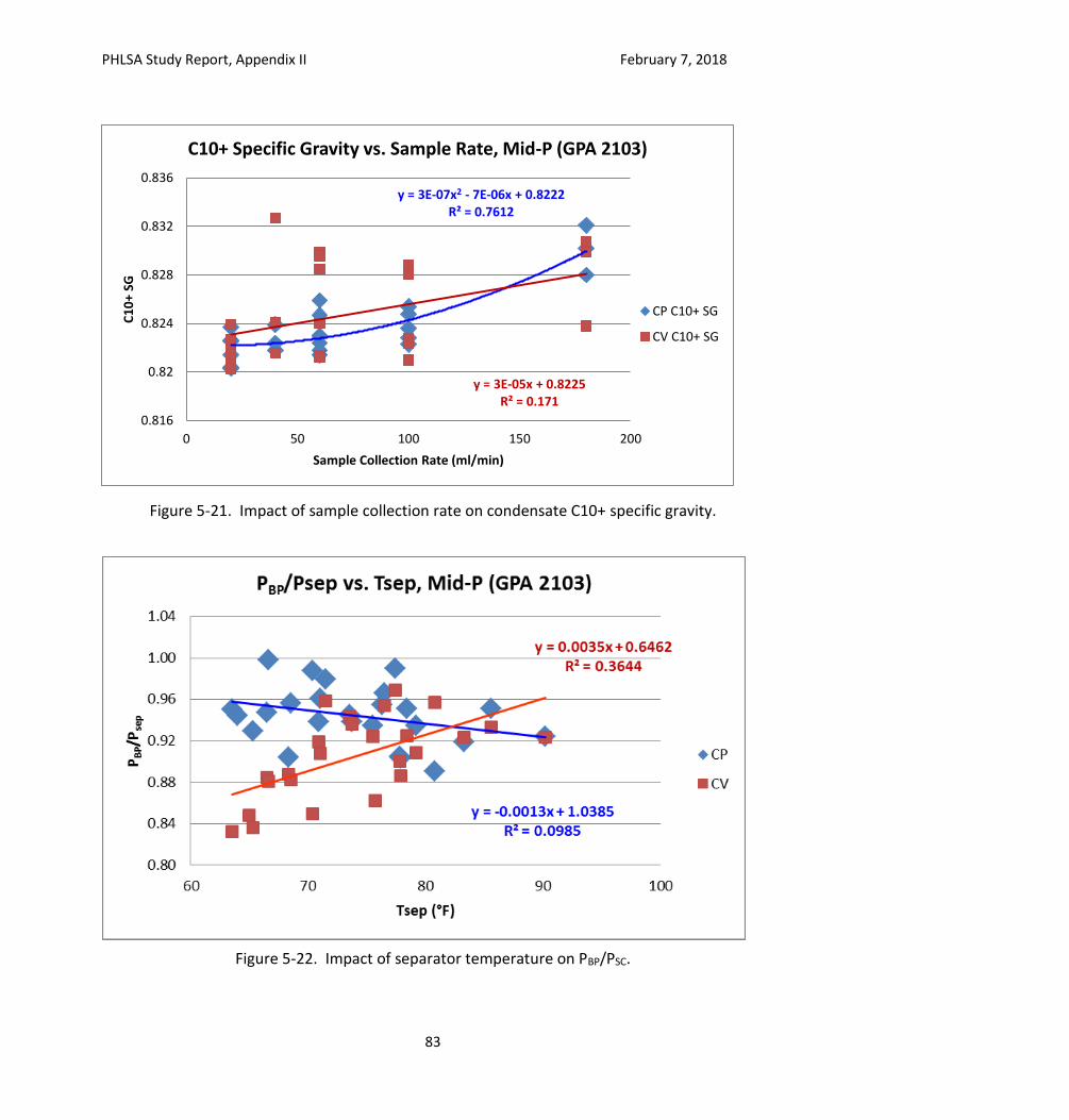
PHLSA Study Report, Appendix II February 7, 2018
83
Figure 5-21. Impact of sample collection rate on condensate C10+ specific gravity.
Figure 5-22. Impact of separator temperature on PBP/PSC.
y = 3E-07x2 - 7E-06x + 0.8222R² = 0.7612
y = 3E-05x + 0.8225R² = 0.171
0.816
0.82
0.824
0.828
0.832
0.836
0 50 100 150 200
C1
0+
SG
Sample Collection Rate (ml/min)
C10+ Specific Gravity vs. Sample Rate, Mid-P (GPA 2103)
CP C10+ SG
CV C10+ SG
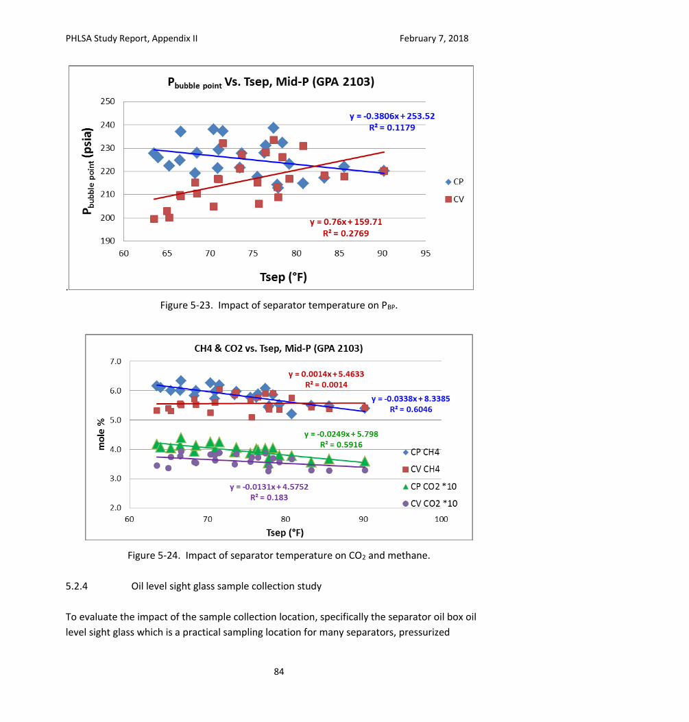
PHLSA Study Report, Appendix II February 7, 2018
84
.
Figure 5-23. Impact of separator temperature on PBP.
Figure 5-24. Impact of separator temperature on CO2 and methane.
5.2.4 Oil level sight glass sample collection study
To evaluate the impact of the sample collection location, specifically the separator oil box oil
level sight glass which is a practical sampling location for many separators, pressurized
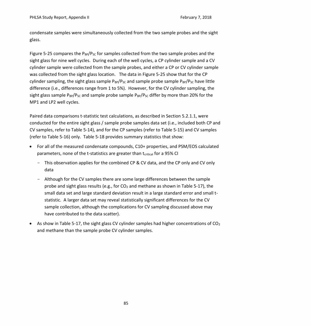
PHLSA Study Report, Appendix II February 7, 2018
85
condensate samples were simultaneously collected from the two sample probes and the sight
glass.
Figure 5-25 compares the PBP/PSC for samples collected from the two sample probes and the
sight glass for nine well cycles. During each of the well cycles, a CP cylinder sample and a CV
cylinder sample were collected from the sample probes, and either a CP or CV cylinder sample
was collected from the sight glass location. The data in Figure 5-25 show that for the CP
cylinder sampling, the sight glass sample PBP/PSC and sample probe sample PBP/PSC have little
difference (i.e., differences range from 1 to 5%). However, for the CV cylinder sampling, the
sight glass sample PBP/PSC and sample probe sample PBP/PSC differ by more than 20% for the
MP1 and LP2 well cycles.
Paired data comparisons t-statistic test calculations, as described in Section 5.2.1.1, were
conducted for the entire sight glass / sample probe samples data set (i.e., included both CP and
CV samples, refer to Table 5-14), and for the CP samples (refer to Table 5-15) and CV samples
(refer to Table 5-16) only. Table 5-18 provides summary statistics that show:
For all of the measured condensate compounds, C10+ properties, and PSM/EOS calculated
parameters, none of the t-statistics are greater than tcritical for a 95% CI
- This observation applies for the combined CP & CV data, and the CP only and CV only
data
- Although for the CV samples there are some large differences between the sample
probe and sight glass results (e.g., for CO2 and methane as shown in Table 5-17), the
small data set and large standard deviation result in a large standard error and small t-
statistic. A larger data set may reveal statistically significant differences for the CV
sample collection, although the complications for CV sampling discussed above may
have contributed to the data scatter).
As show in Table 5-17, the sight glass CV cylinder samples had higher concentrations of CO2
and methane than the sample probe CV cylinder samples.
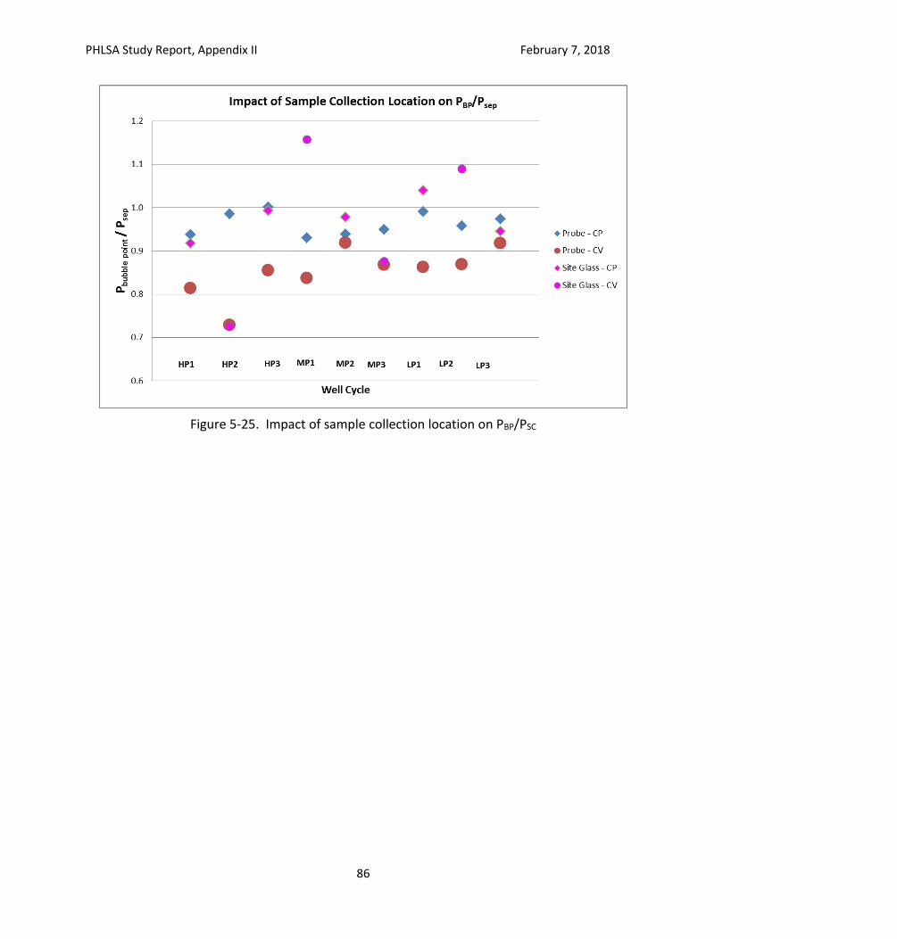
PHLSA Study Report, Appendix II February 7, 2018
86
Figure 5-25. Impact of sample collection location on PBP/PSC
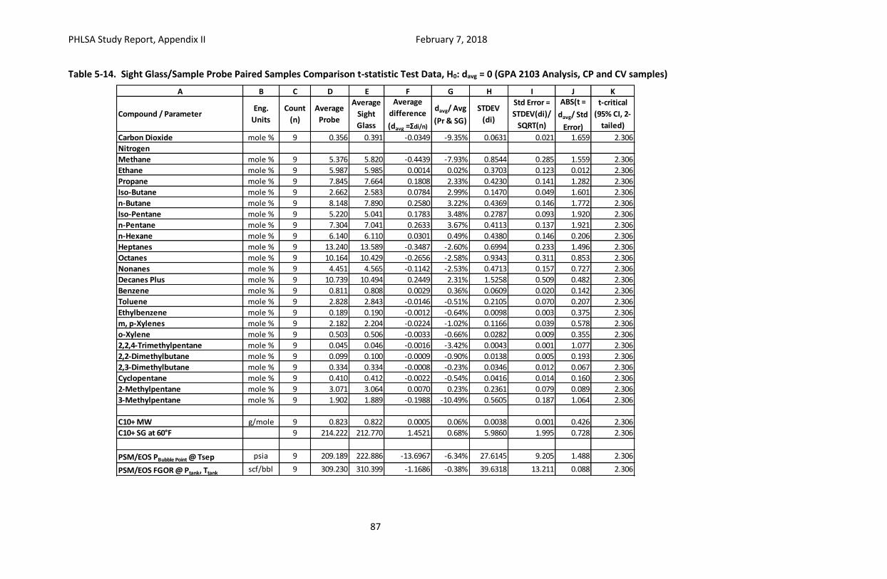
PHLSA Study Report, Appendix II February 7, 2018
87
Table 5-14. Sight Glass/Sample Probe Paired Samples Comparison t-statistic Test Data, H0: davg = 0 (GPA 2103 Analysis, CP and CV samples)
A B C D E F G H I J K
Compound / ParameterEng.
Units
Count
(n)
Average
Probe
Average
Sight
Glass
Average
difference
(davg =Σdi/n)
davg/ Avg
(Pr & SG)
STDEV
(di)
Std Error =
STDEV(di)/
SQRT(n)
ABS(t =
davg/ Std
Error)
t-critical
(95% CI, 2-
tailed)
Carbon Dioxide mole % 9 0.356 0.391 -0.0349 -9.35% 0.0631 0.021 1.659 2.306
Nitrogen
Methane mole % 9 5.376 5.820 -0.4439 -7.93% 0.8544 0.285 1.559 2.306
Ethane mole % 9 5.987 5.985 0.0014 0.02% 0.3703 0.123 0.012 2.306
Propane mole % 9 7.845 7.664 0.1808 2.33% 0.4230 0.141 1.282 2.306
Iso-Butane mole % 9 2.662 2.583 0.0784 2.99% 0.1470 0.049 1.601 2.306
n-Butane mole % 9 8.148 7.890 0.2580 3.22% 0.4369 0.146 1.772 2.306
Iso-Pentane mole % 9 5.220 5.041 0.1783 3.48% 0.2787 0.093 1.920 2.306
n-Pentane mole % 9 7.304 7.041 0.2633 3.67% 0.4113 0.137 1.921 2.306
n-Hexane mole % 9 6.140 6.110 0.0301 0.49% 0.4380 0.146 0.206 2.306
Heptanes mole % 9 13.240 13.589 -0.3487 -2.60% 0.6994 0.233 1.496 2.306
Octanes mole % 9 10.164 10.429 -0.2656 -2.58% 0.9343 0.311 0.853 2.306
Nonanes mole % 9 4.451 4.565 -0.1142 -2.53% 0.4713 0.157 0.727 2.306
Decanes Plus mole % 9 10.739 10.494 0.2449 2.31% 1.5258 0.509 0.482 2.306
Benzene mole % 9 0.811 0.808 0.0029 0.36% 0.0609 0.020 0.142 2.306
Toluene mole % 9 2.828 2.843 -0.0146 -0.51% 0.2105 0.070 0.207 2.306
Ethylbenzene mole % 9 0.189 0.190 -0.0012 -0.64% 0.0098 0.003 0.375 2.306
m, p-Xylenes mole % 9 2.182 2.204 -0.0224 -1.02% 0.1166 0.039 0.578 2.306
o-Xylene mole % 9 0.503 0.506 -0.0033 -0.66% 0.0282 0.009 0.355 2.306
2,2,4-Trimethylpentane mole % 9 0.045 0.046 -0.0016 -3.42% 0.0043 0.001 1.077 2.306
2,2-Dimethylbutane mole % 9 0.099 0.100 -0.0009 -0.90% 0.0138 0.005 0.193 2.306
2,3-Dimethylbutane mole % 9 0.334 0.334 -0.0008 -0.23% 0.0346 0.012 0.067 2.306
Cyclopentane mole % 9 0.410 0.412 -0.0022 -0.54% 0.0416 0.014 0.160 2.306
2-Methylpentane mole % 9 3.071 3.064 0.0070 0.23% 0.2361 0.079 0.089 2.306
3-Methylpentane mole % 9 1.902 1.889 -0.1988 -10.49% 0.5605 0.187 1.064 2.306
C10+ MW g/mole 9 0.823 0.822 0.0005 0.06% 0.0038 0.001 0.426 2.306
C10+ SG at 60°F 9 214.222 212.770 1.4521 0.68% 5.9860 1.995 0.728 2.306
PSM/EOS PBubble Point @ Tsep psia 9 209.189 222.886 -13.6967 -6.34% 27.6145 9.205 1.488 2.306
PSM/EOS FGOR @ Ptank, Ttank scf/bbl 9 309.230 310.399 -1.1686 -0.38% 39.6318 13.211 0.088 2.306
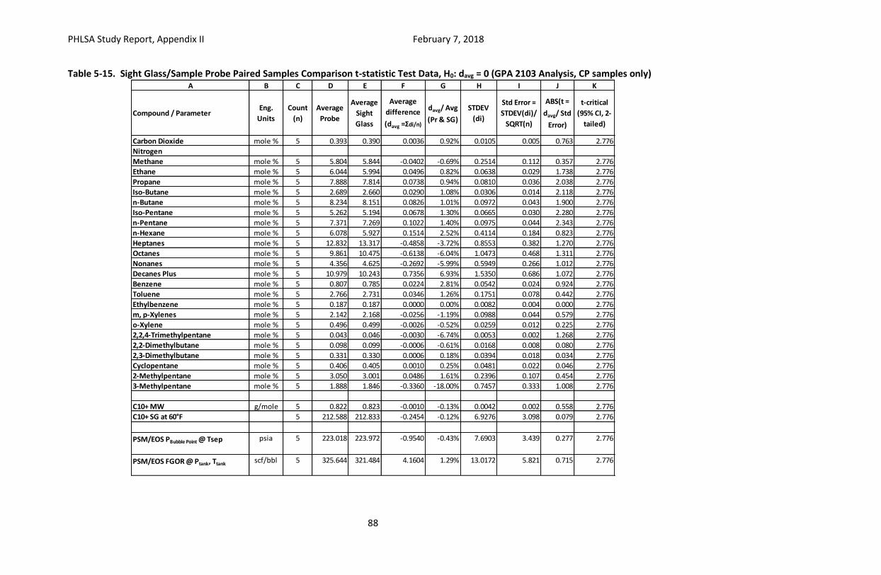
PHLSA Study Report, Appendix II February 7, 2018
88
Table 5-15. Sight Glass/Sample Probe Paired Samples Comparison t-statistic Test Data, H0: davg = 0 (GPA 2103 Analysis, CP samples only)
A B C D E F G H I J K
Compound / ParameterEng.
Units
Count
(n)
Average
Probe
Average
Sight
Glass
Average
difference
(davg =Σdi/n)
davg/ Avg
(Pr & SG)
STDEV
(di)
Std Error =
STDEV(di)/
SQRT(n)
ABS(t =
davg/ Std
Error)
t-critical
(95% CI, 2-
tailed)
Carbon Dioxide mole % 5 0.393 0.390 0.0036 0.92% 0.0105 0.005 0.763 2.776
Nitrogen
Methane mole % 5 5.804 5.844 -0.0402 -0.69% 0.2514 0.112 0.357 2.776
Ethane mole % 5 6.044 5.994 0.0496 0.82% 0.0638 0.029 1.738 2.776
Propane mole % 5 7.888 7.814 0.0738 0.94% 0.0810 0.036 2.038 2.776
Iso-Butane mole % 5 2.689 2.660 0.0290 1.08% 0.0306 0.014 2.118 2.776
n-Butane mole % 5 8.234 8.151 0.0826 1.01% 0.0972 0.043 1.900 2.776
Iso-Pentane mole % 5 5.262 5.194 0.0678 1.30% 0.0665 0.030 2.280 2.776
n-Pentane mole % 5 7.371 7.269 0.1022 1.40% 0.0975 0.044 2.343 2.776
n-Hexane mole % 5 6.078 5.927 0.1514 2.52% 0.4114 0.184 0.823 2.776
Heptanes mole % 5 12.832 13.317 -0.4858 -3.72% 0.8553 0.382 1.270 2.776
Octanes mole % 5 9.861 10.475 -0.6138 -6.04% 1.0473 0.468 1.311 2.776
Nonanes mole % 5 4.356 4.625 -0.2692 -5.99% 0.5949 0.266 1.012 2.776
Decanes Plus mole % 5 10.979 10.243 0.7356 6.93% 1.5350 0.686 1.072 2.776
Benzene mole % 5 0.807 0.785 0.0224 2.81% 0.0542 0.024 0.924 2.776
Toluene mole % 5 2.766 2.731 0.0346 1.26% 0.1751 0.078 0.442 2.776
Ethylbenzene mole % 5 0.187 0.187 0.0000 0.00% 0.0082 0.004 0.000 2.776
m, p-Xylenes mole % 5 2.142 2.168 -0.0256 -1.19% 0.0988 0.044 0.579 2.776
o-Xylene mole % 5 0.496 0.499 -0.0026 -0.52% 0.0259 0.012 0.225 2.776
2,2,4-Trimethylpentane mole % 5 0.043 0.046 -0.0030 -6.74% 0.0053 0.002 1.268 2.776
2,2-Dimethylbutane mole % 5 0.098 0.099 -0.0006 -0.61% 0.0168 0.008 0.080 2.776
2,3-Dimethylbutane mole % 5 0.331 0.330 0.0006 0.18% 0.0394 0.018 0.034 2.776
Cyclopentane mole % 5 0.406 0.405 0.0010 0.25% 0.0481 0.022 0.046 2.776
2-Methylpentane mole % 5 3.050 3.001 0.0486 1.61% 0.2396 0.107 0.454 2.776
3-Methylpentane mole % 5 1.888 1.846 -0.3360 -18.00% 0.7457 0.333 1.008 2.776
C10+ MW g/mole 5 0.822 0.823 -0.0010 -0.13% 0.0042 0.002 0.558 2.776
C10+ SG at 60°F 5 212.588 212.833 -0.2454 -0.12% 6.9276 3.098 0.079 2.776
PSM/EOS PBubble Point @ Tsep psia 5 223.018 223.972 -0.9540 -0.43% 7.6903 3.439 0.277 2.776
PSM/EOS FGOR @ Ptank, Ttank scf/bbl 5 325.644 321.484 4.1604 1.29% 13.0172 5.821 0.715 2.776
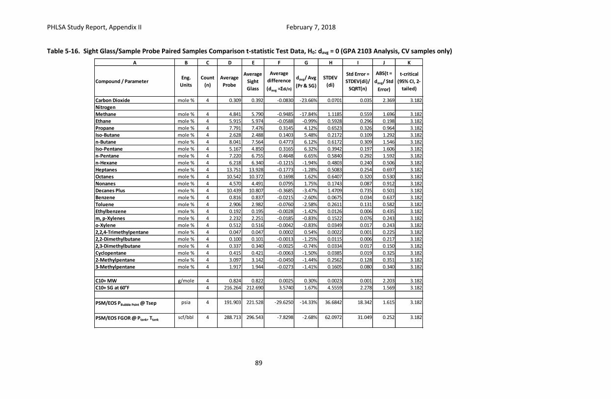
PHLSA Study Report, Appendix II February 7, 2018
89
Table 5-16. Sight Glass/Sample Probe Paired Samples Comparison t-statistic Test Data, H0: davg = 0 (GPA 2103 Analysis, CV samples only)
A B C D E F G H I J K
Compound / ParameterEng.
Units
Count
(n)
Average
Probe
Average
Sight
Glass
Average
difference
(davg =Σdi/n)
davg/ Avg
(Pr & SG)
STDEV
(di)
Std Error =
STDEV(di)/
SQRT(n)
ABS(t =
davg/ Std
Error)
t-critical
(95% CI, 2-
tailed)
Carbon Dioxide mole % 4 0.309 0.392 -0.0830 -23.66% 0.0701 0.035 2.369 3.182
Nitrogen
Methane mole % 4 4.841 5.790 -0.9485 -17.84% 1.1185 0.559 1.696 3.182
Ethane mole % 4 5.915 5.974 -0.0588 -0.99% 0.5928 0.296 0.198 3.182
Propane mole % 4 7.791 7.476 0.3145 4.12% 0.6523 0.326 0.964 3.182
Iso-Butane mole % 4 2.628 2.488 0.1403 5.48% 0.2172 0.109 1.292 3.182
n-Butane mole % 4 8.041 7.564 0.4773 6.12% 0.6172 0.309 1.546 3.182
Iso-Pentane mole % 4 5.167 4.850 0.3165 6.32% 0.3942 0.197 1.606 3.182
n-Pentane mole % 4 7.220 6.755 0.4648 6.65% 0.5840 0.292 1.592 3.182
n-Hexane mole % 4 6.218 6.340 -0.1215 -1.94% 0.4803 0.240 0.506 3.182
Heptanes mole % 4 13.751 13.928 -0.1773 -1.28% 0.5083 0.254 0.697 3.182
Octanes mole % 4 10.542 10.372 0.1698 1.62% 0.6407 0.320 0.530 3.182
Nonanes mole % 4 4.570 4.491 0.0795 1.75% 0.1743 0.087 0.912 3.182
Decanes Plus mole % 4 10.439 10.807 -0.3685 -3.47% 1.4709 0.735 0.501 3.182
Benzene mole % 4 0.816 0.837 -0.0215 -2.60% 0.0675 0.034 0.637 3.182
Toluene mole % 4 2.906 2.982 -0.0760 -2.58% 0.2611 0.131 0.582 3.182
Ethylbenzene mole % 4 0.192 0.195 -0.0028 -1.42% 0.0126 0.006 0.435 3.182
m, p-Xylenes mole % 4 2.232 2.251 -0.0185 -0.83% 0.1522 0.076 0.243 3.182
o-Xylene mole % 4 0.512 0.516 -0.0042 -0.83% 0.0349 0.017 0.243 3.182
2,2,4-Trimethylpentane mole % 4 0.047 0.047 0.0002 0.54% 0.0022 0.001 0.225 3.182
2,2-Dimethylbutane mole % 4 0.100 0.101 -0.0013 -1.25% 0.0115 0.006 0.217 3.182
2,3-Dimethylbutane mole % 4 0.337 0.340 -0.0025 -0.74% 0.0334 0.017 0.150 3.182
Cyclopentane mole % 4 0.415 0.421 -0.0063 -1.50% 0.0385 0.019 0.325 3.182
2-Methylpentane mole % 4 3.097 3.142 -0.0450 -1.44% 0.2562 0.128 0.351 3.182
3-Methylpentane mole % 4 1.917 1.944 -0.0273 -1.41% 0.1605 0.080 0.340 3.182
C10+ MW g/mole 4 0.824 0.822 0.0025 0.30% 0.0023 0.001 2.203 3.182
C10+ SG at 60°F 4 216.264 212.690 3.5740 1.67% 4.5559 2.278 1.569 3.182
PSM/EOS PBubble Point @ Tsep psia 4 191.903 221.528 -29.6250 -14.33% 36.6842 18.342 1.615 3.182
PSM/EOS FGOR @ Ptank, Ttank scf/bbl 4 288.713 296.543 -7.8298 -2.68% 62.0972 31.049 0.252 3.182
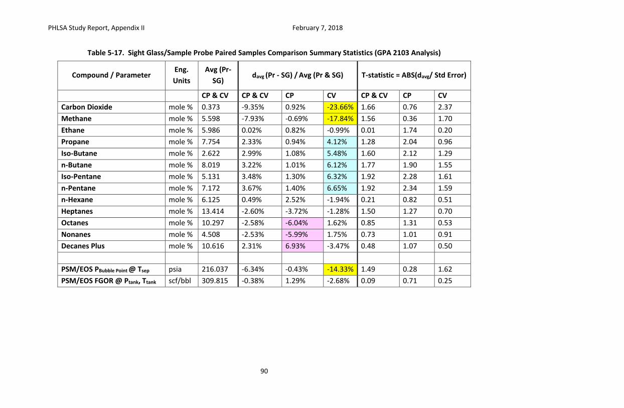
PHLSA Study Report, Appendix II February 7, 2018
90
Table 5-17. Sight Glass/Sample Probe Paired Samples Comparison Summary Statistics (GPA 2103 Analysis)
Compound / Parameter Eng.
Units
Avg (Pr-
SG) davg (Pr - SG) / Avg (Pr & SG) T-statistic = ABS(davg/ Std Error)
CP & CV CP & CV CP CV CP & CV CP CV
Carbon Dioxide mole % 0.373 -9.35% 0.92% -23.66% 1.66 0.76 2.37
Methane mole % 5.598 -7.93% -0.69% -17.84% 1.56 0.36 1.70
Ethane mole % 5.986 0.02% 0.82% -0.99% 0.01 1.74 0.20
Propane mole % 7.754 2.33% 0.94% 4.12% 1.28 2.04 0.96
Iso-Butane mole % 2.622 2.99% 1.08% 5.48% 1.60 2.12 1.29
n-Butane mole % 8.019 3.22% 1.01% 6.12% 1.77 1.90 1.55
Iso-Pentane mole % 5.131 3.48% 1.30% 6.32% 1.92 2.28 1.61
n-Pentane mole % 7.172 3.67% 1.40% 6.65% 1.92 2.34 1.59
n-Hexane mole % 6.125 0.49% 2.52% -1.94% 0.21 0.82 0.51
Heptanes mole % 13.414 -2.60% -3.72% -1.28% 1.50 1.27 0.70
Octanes mole % 10.297 -2.58% -6.04% 1.62% 0.85 1.31 0.53
Nonanes mole % 4.508 -2.53% -5.99% 1.75% 0.73 1.01 0.91
Decanes Plus mole % 10.616 2.31% 6.93% -3.47% 0.48 1.07 0.50
PSM/EOS PBubble Point @ Tsep psia 216.037 -6.34% -0.43% -14.33% 1.49 0.28 1.62
PSM/EOS FGOR @ Ptank, Ttank scf/bbl 309.815 -0.38% 1.29% -2.68% 0.09 0.71 0.25
PHLSA Study Report, Appendix II February 7, 2018
91
6. Process Measurement
Supporting data and calculations for the information presented in this section can be found in
Annex 5 and Appendix IV.4
6.1 Introduction
Several instruments were used to measure process parameters during the PHLSA study.
Manufacturer metrological specifications and calibration data, when available, were typically
used for measurement uncertainty calculations.
An integrated operational map, which identifies and codifies each instrument in the process
measurement system, may be consulted in Appendix IV.
This section includes two parts. The first refers to general instrumentation, such as
temperature, pressure and liquid level transducers. All signals are processed in a Supervisory
Control and Data Acquisition (SCADA) system with an Analog-to-Digital (A-D) converter and
recorded in a data logger. Total uncertainty for each measurement (i.e., combination of data
logger and instrumentation uncertainties) was calculated from transducer and Electronic Flow
Computer (EFC) accuracy information. The calculation of uncertainties for measurements
based on several instruments, such as tank pressure one foot from the bottom, are discussed at
the end of this section.
The second part of this section addresses flow measurements. Liquid process meters were
calibrated to accuracies compliant with custody transfer limits for steady-state flow and
operate under a metrological confirmation process that includes field proving. The associated
uncertainties are the lower feasible for midstream operations. Because the various gas meters
used for this project have different operating principles, they require specific uncertainty
calculations. A flow computer records readings of flow meters, and because they are digital
signals the influence of the data logger on measurement uncertainty is null.
Section 6.2 provides general information regarding calibration and accuracy data for process
measurement instruments used for this study, and the methodology used to estimate
measurement uncertainty based on this information. Many of these calibrations and accuracy
specifications only apply under prescribed conditions (e.g., steady-state flow of a fluid of known
composition); thus, for some instruments, engineering assumptions were made regarding
instrument/measurement uncertainty for subsequent uncertainty estimation calculations.
These engineering estimates are documented in Section 8.
PHLSA Study Report, Appendix II February 7, 2018
92
6.2 Uncertainty of General Process Instrumentation
6.2.1 Description of sources of uncertainty4
Temperature transducers. Instruments from several manufacturers were used and typical
accuracy is in the range of 1.5 to 2 degrees Fahrenheit.
Pressure transducers. Instruments from various manufactures and with differing accuracies
were used with +/- 2% of the measured value a typical accuracy specification.
Liquid tank height. Tank ullage is measured by an instrument with a manufacturer stated
accuracy of 0.125 inches.
Liquid density. Stabilized condensate (i.e., tank liquids) density was determined using a liquid densitometer with accuracy better than 0.1 %. This measurement was conducted in the laboratory. The Coriolis meter recorded flowing density.
Flow computer. Transducer signals are processed by a flow computer with an ADC with 0.2 %
measurement accuracy for analogic transducer signals.
Appendix IV.4 provides additional details regarding the instruments operating principles and
calibrations.
6.2.2 General uncertainty model
The signals of some instruments were field verified using a calibration procedure that measured
instrument output power or current, because these units do not correspond to the measured
property, such as temperature or pressure (e.g. mV output vs. °F measured parameter). Such
calibrations only confirm instrument functionality, and manufacturer accuracy specifications
were used for uncertainty calculations.
A 95% confidence level (API MPMS 13.1 5.3) was the basis for uncertainty calculations. A
rectangular distribution (API MPMS 13.3 4.18.4) was assumed for most instrument calibrations.
The 95% CI coverage factor for the standard uncertainty corresponds to 1.65 for rectangular
distributions and 1.96 for normal distributions.
4 The documentation for the referenced instrument accuracies are in the project Calibration Report, Appendix IV.4.
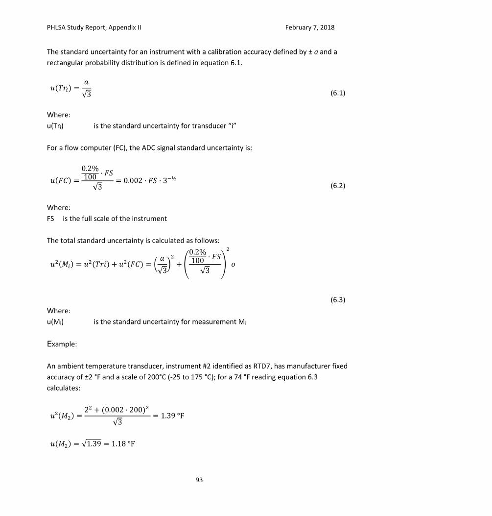
PHLSA Study Report, Appendix II February 7, 2018
93
The standard uncertainty for an instrument with a calibration accuracy defined by ± a and a
rectangular probability distribution is defined in equation 6.1.
𝑢(𝑇𝑟𝑖) =𝑎
√3
(6.1)
Where:
u(Tri) is the standard uncertainty for transducer “i”
For a flow computer (FC), the ADC signal standard uncertainty is:
𝑢(𝐹𝐶) =
0.2%100 · 𝐹𝑆
√3= 0.002 · 𝐹𝑆 · 3−½
(6.2)
Where:
FS is the full scale of the instrument
The total standard uncertainty is calculated as follows:
𝑢2(𝑀𝑖) = 𝑢2(𝑇𝑟𝑖) + 𝑢2(𝐹𝐶) = (𝑎
√3)2
+ (
0.2%100 · 𝐹𝑆
√3)
2
𝑜
(6.3)
Where:
u(Mi) is the standard uncertainty for measurement Mi
Example:
An ambient temperature transducer, instrument #2 identified as RTD7, has manufacturer fixed
accuracy of ±2 °F and a scale of 200°C (-25 to 175 °C); for a 74 °F reading equation 6.3
calculates:
𝑢²(𝑀2) =22 + (0.002 · 200)²
√3= 1.39 °F
𝑢(𝑀2) = √1.39 = 1.18 °F
PHLSA Study Report, Appendix II February 7, 2018
94
𝑈(𝑀2) = 1.18 · 1.65 = 2.56 °F
(6.4)
%𝑈(𝑀2) =2.56
74= 2.62%
(6.5)
Table 6-1 summarizes process instrumentation uncertainties, and relative uncertainties are for
information purposes only. For the testing, relative uncertainties were calculated based on
actual measurements.
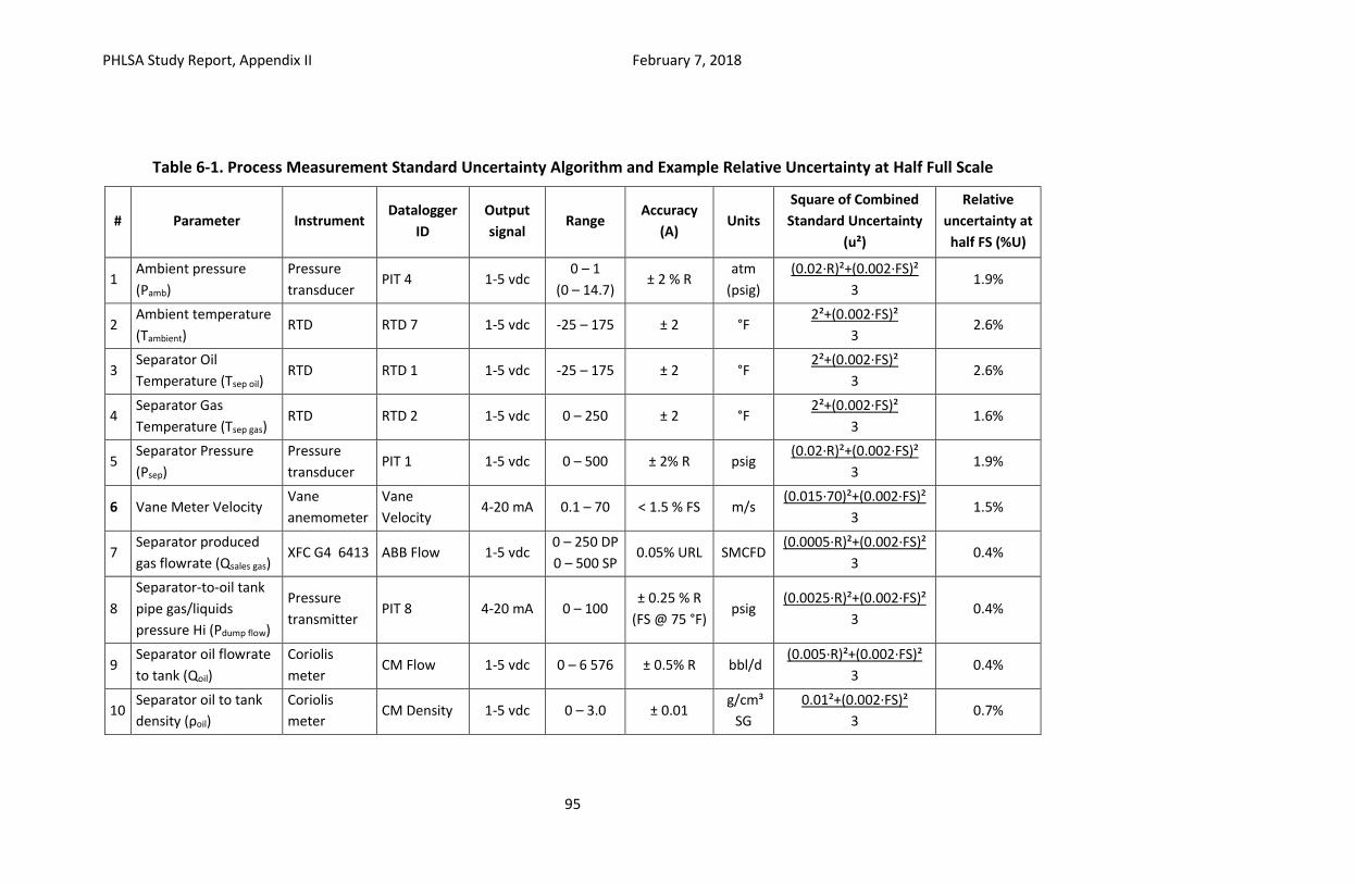
PHLSA Study Report, Appendix II February 7, 2018
95
Table 6-1. Process Measurement Standard Uncertainty Algorithm and Example Relative Uncertainty at Half Full Scale
# Parameter Instrument Datalogger
ID
Output
signal Range
Accuracy
(A) Units
Square of Combined
Standard Uncertainty
(u²)
Relative
uncertainty at
half FS (%U)
1 Ambient pressure
(Pamb)
Pressure
transducer PIT 4 1-5 vdc
0 – 1
(0 – 14.7) ± 2 % R
atm
(psig)
(0.02·R)²+(0.002·FS)²
3 1.9%
2 Ambient temperature
(Tambient) RTD RTD 7 1-5 vdc -25 – 175 ± 2 °F
2²+(0.002·FS)²
3 2.6%
3 Separator Oil
Temperature (Tsep oil) RTD RTD 1 1-5 vdc -25 – 175 ± 2 °F
2²+(0.002·FS)²
3 2.6%
4 Separator Gas
Temperature (Tsep gas) RTD RTD 2 1-5 vdc 0 – 250 ± 2 °F
2²+(0.002·FS)²
3 1.6%
5 Separator Pressure
(Psep)
Pressure
transducer PIT 1 1-5 vdc 0 – 500 ± 2% R psig
(0.02·R)²+(0.002·FS)²
3 1.9%
6 Vane Meter Velocity Vane
anemometer
Vane
Velocity 4-20 mA 0.1 – 70 < 1.5 % FS m/s
(0.015·70)²+(0.002·FS)²
3 1.5%
7 Separator produced
gas flowrate (Qsales gas) XFC G4 6413 ABB Flow 1-5 vdc
0 – 250 DP
0 – 500 SP 0.05% URL SMCFD
(0.0005·R)²+(0.002·FS)²
3 0.4%
8
Separator-to-oil tank
pipe gas/liquids
pressure Hi (Pdump flow)
Pressure
transmitter PIT 8 4-20 mA 0 – 100
± 0.25 % R
(FS @ 75 °F) psig
(0.0025·R)²+(0.002·FS)²
3 0.4%
9 Separator oil flowrate
to tank (Qoil)
Coriolis
meter CM Flow 1-5 vdc 0 – 6 576 ± 0.5% R bbl/d
(0.005·R)²+(0.002·FS)²
3 0.4%
10 Separator oil to tank
density (ρoil)
Coriolis
meter CM Density 1-5 vdc 0 – 3.0 ± 0.01
g/cm³
SG
0.01²+(0.002·FS)²
3 0.7%
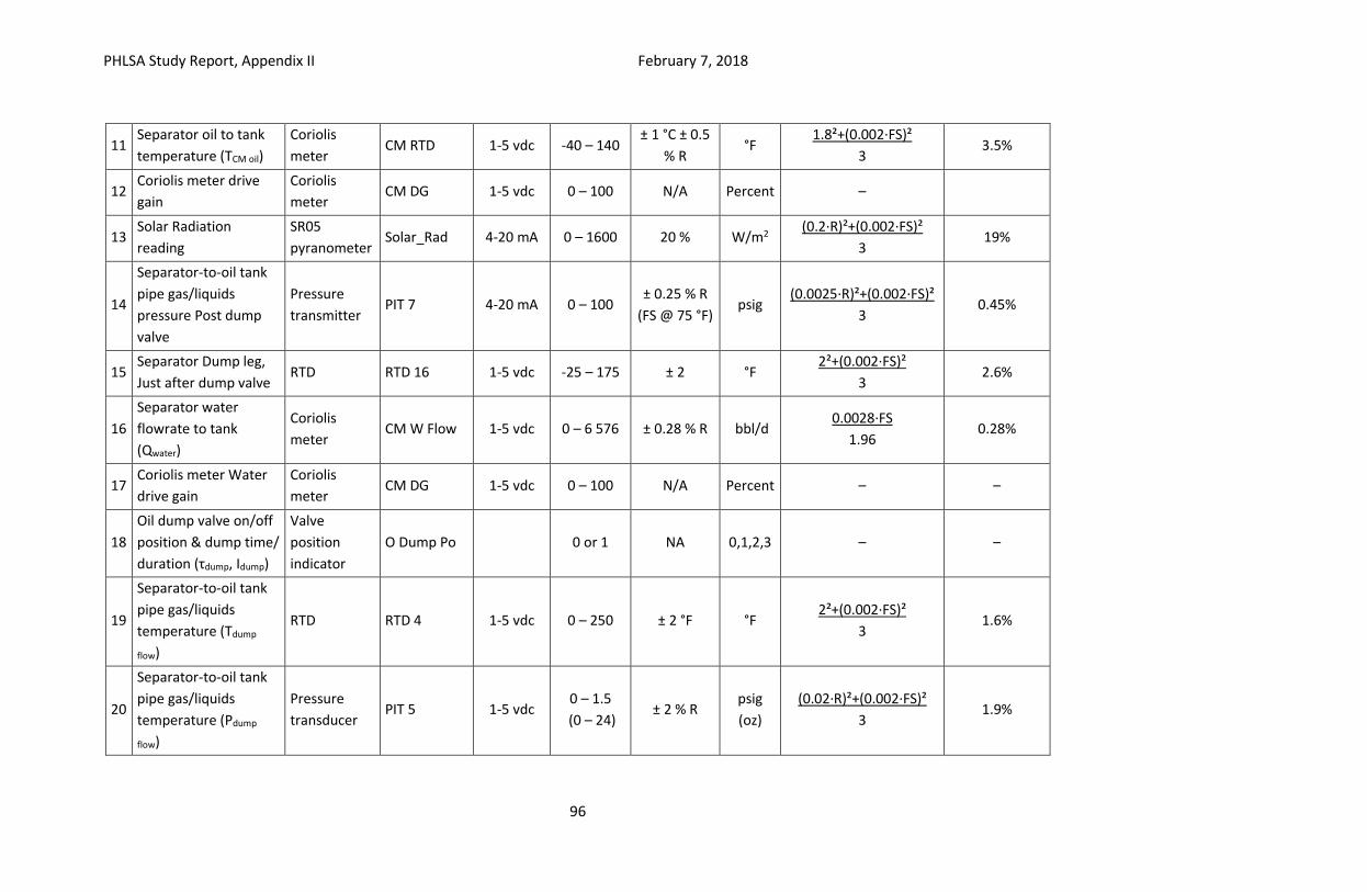
PHLSA Study Report, Appendix II February 7, 2018
96
11 Separator oil to tank
temperature (TCM oil)
Coriolis
meter CM RTD 1-5 vdc -40 – 140
± 1 °C ± 0.5
% R °F
1.8²+(0.002·FS)²
3 3.5%
12 Coriolis meter drive
gain
Coriolis
meter CM DG 1-5 vdc 0 – 100 N/A Percent –
13 Solar Radiation
reading
SR05
pyranometer Solar_Rad 4-20 mA 0 – 1600 20 % W/m2
(0.2·R)²+(0.002·FS)²
3 19%
14
Separator-to-oil tank
pipe gas/liquids
pressure Post dump
valve
Pressure
transmitter PIT 7 4-20 mA 0 – 100
± 0.25 % R
(FS @ 75 °F) psig
(0.0025·R)²+(0.002·FS)²
3 0.45%
15 Separator Dump leg,
Just after dump valve RTD RTD 16 1-5 vdc -25 – 175 ± 2 °F
2²+(0.002·FS)²
3 2.6%
16
Separator water
flowrate to tank
(Qwater)
Coriolis
meter CM W Flow 1-5 vdc 0 – 6 576 ± 0.28 % R bbl/d
0.0028·FS
1.96 0.28%
17 Coriolis meter Water
drive gain
Coriolis
meter CM DG 1-5 vdc 0 – 100 N/A Percent – –
18
Oil dump valve on/off
position & dump time/
duration (τdump, Idump)
Valve
position
indicator
O Dump Po 0 or 1 NA 0,1,2,3 – –
19
Separator-to-oil tank
pipe gas/liquids
temperature (Tdump
flow)
RTD RTD 4 1-5 vdc 0 – 250 ± 2 °F °F 2²+(0.002·FS)²
3 1.6%
20
Separator-to-oil tank
pipe gas/liquids
temperature (Pdump
flow)
Pressure
transducer PIT 5 1-5 vdc
0 – 1.5
(0 – 24) ± 2 % R
psig
(oz)
(0.02·R)²+(0.002·FS)²
3 1.9%
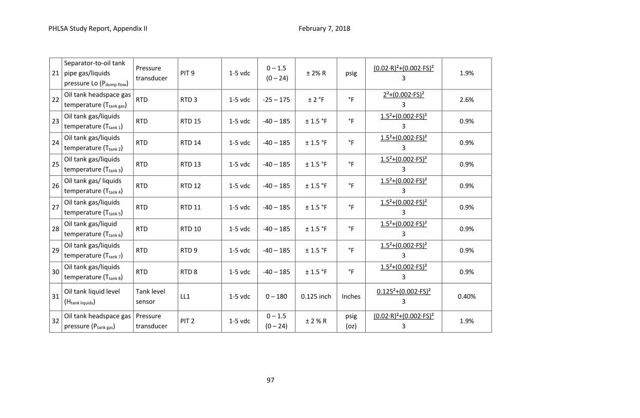
PHLSA Study Report, Appendix II February 7, 2018
97
21
Separator-to-oil tank
pipe gas/liquids
pressure Lo (Pdump flow)
Pressure
transducer PIT 9 1-5 vdc
0 – 1.5
(0 – 24) ± 2% R psig
(0.02·R)²+(0.002·FS)²
3 1.9%
22 Oil tank headspace gas
temperature (Ttank gas) RTD RTD 3 1-5 vdc -25 – 175 ± 2 °F °F
2²+(0.002·FS)²
3 2.6%
23 Oil tank gas/liquids
temperature (Ttank 1) RTD RTD 15 1-5 vdc -40 – 185 ± 1.5 °F °F
1.5²+(0.002·FS)²
3 0.9%
24 Oil tank gas/liquids
temperature (Ttank 2) RTD RTD 14 1-5 vdc -40 – 185 ± 1.5 °F °F
1.5²+(0.002·FS)²
3 0.9%
25 Oil tank gas/liquids
temperature (Ttank 3) RTD RTD 13 1-5 vdc -40 – 185 ± 1.5 °F °F
1.5²+(0.002·FS)²
3 0.9%
26 Oil tank gas/ liquids
temperature (Ttank 4) RTD RTD 12 1-5 vdc -40 – 185 ± 1.5 °F °F
1.5²+(0.002·FS)²
3 0.9%
27 Oil tank gas/liquids
temperature (Ttank 5) RTD RTD 11 1-5 vdc -40 – 185 ± 1.5 °F °F
1.5²+(0.002·FS)²
3 0.9%
28 Oil tank gas/liquid
temperature (Ttank 6) RTD RTD 10 1-5 vdc -40 – 185 ± 1.5 °F °F
1.5²+(0.002·FS)²
3 0.9%
29 Oil tank gas/liquids
temperature (Ttank 7) RTD RTD 9 1-5 vdc -40 – 185 ± 1.5 °F °F
1.5²+(0.002·FS)²
3 0.9%
30 Oil tank gas/liquids
temperature (Ttank 8) RTD RTD 8 1-5 vdc -40 – 185 ± 1.5 °F °F
1.5²+(0.002·FS)²
3 0.9%
31 Oil tank liquid level
(Htank liquids)
Tank level
sensor LL1 1-5 vdc 0 – 180 0.125 inch Inches
0.125²+(0.002·FS)²
3 0.40%
32 Oil tank headspace gas
pressure (Ptank gas)
Pressure
transducer PIT 2 1-5 vdc
0 – 1.5
(0 – 24) ± 2 % R
psig
(oz)
(0.02·R)²+(0.002·FS)²
3 1.9%
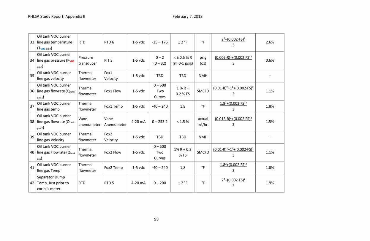
PHLSA Study Report, Appendix II February 7, 2018
98
33
Oil tank VOC burner
line gas temperature
(TVOC pipe)
RTD RTD 6 1-5 vdc -25 – 175 ± 2 °F °F 2²+(0.002·FS)²
3 2.6%
34
Oil tank VOC burner
line gas pressure (PVOC
pipe)
Pressure
transducer PIT 3 1-5 vdc
0 – 2
(0 – 32)
< ± 0.5 % R
(@ 0-1 psig)
psig
(oz)
(0.005·R)²+(0.002·FS)²
3 0.6%
35 Oil tank VOC burner
line gas velocity
Thermal
flowmeter
Fox1
Velocity 1-5 vdc TBD TBD NMH –
36
Oil tank VOC burner
line gas flowrate (Qtank
gas 1)
Thermal
flowmeter Fox1 Flow 1-5 vdc
0 – 500
Two
Curves
1 % R +
0.2 % FS SMCFD
(0.01·R)²+1²+(0.002·FS)²
3 1.1%
37 Oil tank VOC burner
line gas temp
Thermal
flowmeter Fox1 Temp 1-5 vdc -40 – 240 1.8 °F
1.8²+(0.002·FS)²
3 1.8%
38
Oil tank VOC burner
line gas flowrate (Qtank
gas 2)
Vane
anemometer
Vane
Anemometer 4-20 mA 0 – 253.2 < 1.5 %
actual
m3/hr.
(0.015·R)²+(0.002·FS)²
3 1.5%
39 Oil tank VOC burner
line gas Velocity
Thermal
flowmeter
Fox2
Velocity 1-5 vdc TBD TBD NMH –
40
Oil tank VOC burner
line gas Flowrate (Qtank
gas)
Thermal
flowmeter Fox2 Flow 1-5 vdc
0 – 500
Two
Curves
1% R + 0.2
% FS SMCFD
(0.01·R)²+1²+(0.002·FS)²
3 1.1%
41 Oil tank VOC burner
line gas Temp
Thermal
flowmeter Fox2 Temp 1-5 vdc -40 – 240 1.8 °F
1.8²+(0.002·FS)²
3 1.8%
42
Separator Dump
Temp, Just prior to
coriolis meter.
RTD RTD 5 4-20 mA 0 – 200 ± 2 °F °F 2²+(0.002·FS)²
3 1.9%
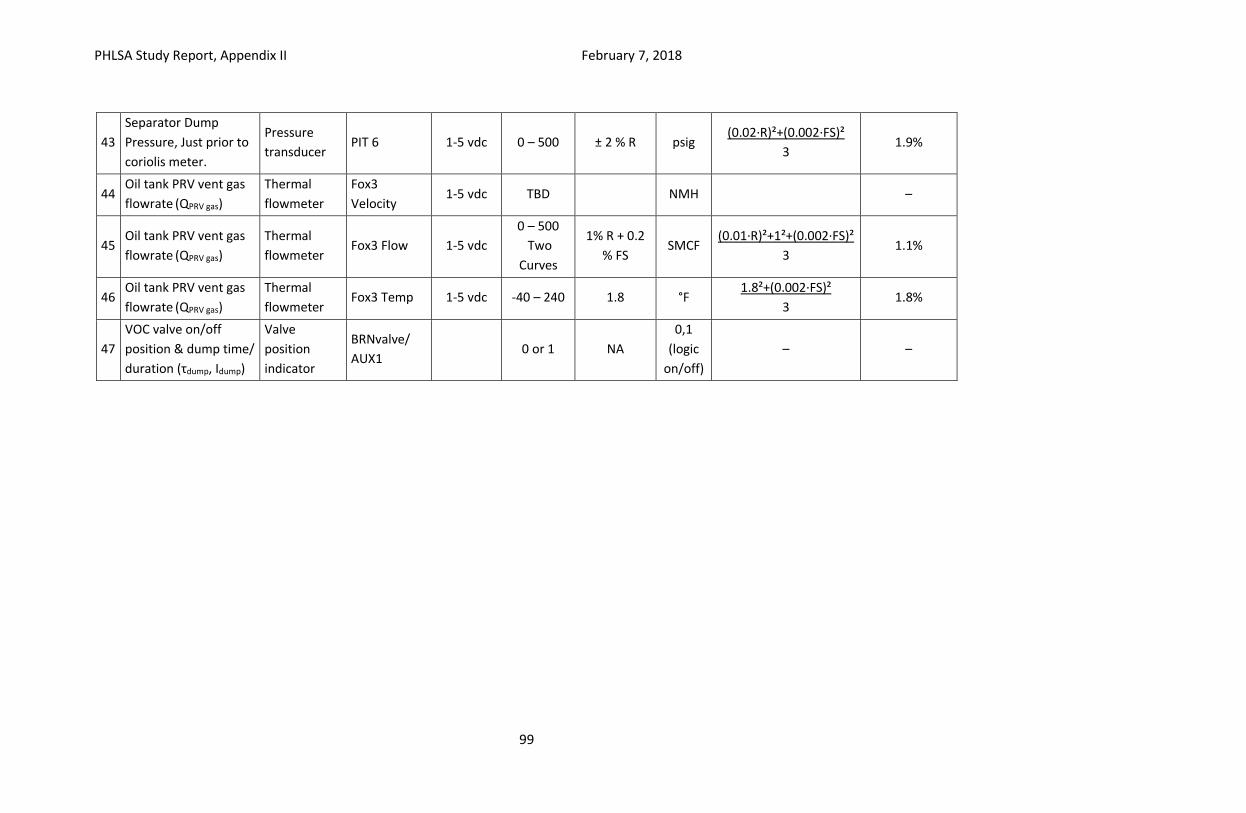
PHLSA Study Report, Appendix II February 7, 2018
99
43
Separator Dump
Pressure, Just prior to
coriolis meter.
Pressure
transducer PIT 6 1-5 vdc 0 – 500 ± 2 % R psig
(0.02·R)²+(0.002·FS)²
3 1.9%
44 Oil tank PRV vent gas
flowrate (QPRV gas)
Thermal
flowmeter
Fox3
Velocity 1-5 vdc TBD NMH –
45 Oil tank PRV vent gas
flowrate (QPRV gas)
Thermal
flowmeter Fox3 Flow 1-5 vdc
0 – 500
Two
Curves
1% R + 0.2
% FS SMCF
(0.01·R)²+1²+(0.002·FS)²
3 1.1%
46 Oil tank PRV vent gas
flowrate (QPRV gas)
Thermal
flowmeter Fox3 Temp 1-5 vdc -40 – 240 1.8 °F
1.8²+(0.002·FS)²
3 1.8%
47
VOC valve on/off
position & dump time/
duration (τdump, Idump)
Valve
position
indicator
BRNvalve/
AUX1 0 or 1 NA
0,1
(logic
on/off)
– –
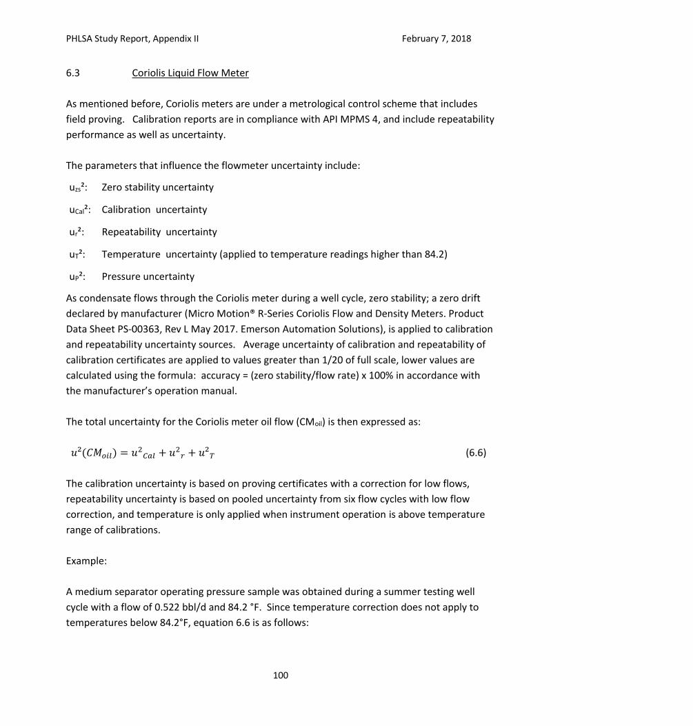
PHLSA Study Report, Appendix II February 7, 2018
100
6.3 Coriolis Liquid Flow Meter
As mentioned before, Coriolis meters are under a metrological control scheme that includes
field proving. Calibration reports are in compliance with API MPMS 4, and include repeatability
performance as well as uncertainty.
The parameters that influence the flowmeter uncertainty include:
uzs²: Zero stability uncertainty
uCal²: Calibration uncertainty
ur²: Repeatability uncertainty
uT²: Temperature uncertainty (applied to temperature readings higher than 84.2)
uP²: Pressure uncertainty
As condensate flows through the Coriolis meter during a well cycle, zero stability; a zero drift
declared by manufacturer (Micro Motion® R-Series Coriolis Flow and Density Meters. Product
Data Sheet PS-00363, Rev L May 2017. Emerson Automation Solutions), is applied to calibration
and repeatability uncertainty sources. Average uncertainty of calibration and repeatability of
calibration certificates are applied to values greater than 1/20 of full scale, lower values are
calculated using the formula: accuracy = (zero stability/flow rate) x 100% in accordance with
the manufacturer’s operation manual.
The total uncertainty for the Coriolis meter oil flow (CMoil) is then expressed as:
𝑢²(𝐶𝑀𝑜𝑖𝑙) = 𝑢2𝐶𝑎𝑙 + 𝑢2
𝑟 + 𝑢²𝑇 (6.6)
The calibration uncertainty is based on proving certificates with a correction for low flows,
repeatability uncertainty is based on pooled uncertainty from six flow cycles with low flow
correction, and temperature is only applied when instrument operation is above temperature
range of calibrations.
Example:
A medium separator operating pressure sample was obtained during a summer testing well
cycle with a flow of 0.522 bbl/d and 84.2 °F. Since temperature correction does not apply to
temperatures below 84.2°F, equation 6.6 is as follows:
PHLSA Study Report, Appendix II February 7, 2018
101
𝑢²(𝐶𝑀𝑜𝑖𝑙) = (0.522 · 0.00026)² + (0.522 · 0.00018)² + (|0| · 5/9 · 0.000875)²)²
= 0.00011
𝑢(𝐶𝑀𝑜𝑖𝑙) = √1.12𝑥10−8 = 0.00011
𝑈(𝐶𝑀𝑜𝑖𝑙) = 0.00011 · 1.96 = 0.0002
%𝑈(𝐶𝑀𝑜𝑖𝑙) = 0.021%
(6.7)
This uncertainty is applicable to steady flows, and because steady flow is not feasible under
field conditions, an uncertainty of 1.0% of flow, twice the manufacturer specification of 0.5 % of
flow, was considered.
PHLSA Study Report, Appendix II February 7, 2018
102
7. Uncertainty of Storage Tank Mass Balance and FGOR Measurements
Data and documentation for these calculations are included in the spreadsheets in Appendix
IV.2.
PHLSA Study Report, Appendix II February 7, 2018
103
8. PSM/EOS FGOR Calculations Uncertainty Analysis
Supporting data and calculations for the information presented in this section can be found in
Appendix V.
8.1 Introduction.
The uncertainties of many measurements conducted for this project were estimated using
methodologies from international standards; however, this is not the case for PSM/EOS
calculations of FGORs.
The uncertainty of results calculated using Equation of State software packages cannot be
determined using standard GUM procedures because calculations of sensitivity coefficients and
combined calculations are not possible for such black box models. Therefore, the uncertainties
of PSM/EOS FGOR calculations were estimated using a numerical approximation method and a
Monte Carlo simulation, and the results of these two approaches were compared.
Numerical approximation sensitivity assessment and uncertainty calculation
One approach to estimate the uncertainty of PSM/EOS calculations of FGOR is to isolate and
vary calculation input variables to determine the sensitivity of the calculation to the parameter.
This numerical approximation solution, or “dither method” described in API MSPS 13.3 5.6.2,
iterates input values over the range of uncertainty for the variable to determine the sensitivity
of the dependent variable (e.g., FGOR) to this variable. Combining these results for all the input
variables provides a reasonable estimate of the overall FGOR uncertainty. This can be a
laborious process and additional complexity can result from combining uncertainty sources; for
example, some may have a normal distribution while others may have triangular or rectangular
distribution.
Monte Carlo simulation sensitivity assessment and uncertainty calculation
Monte Carlo (MC) simulation is another sensitivity and uncertainty calculation approach, but it
can be limited by availability of technical resources, software and hardware tools. Monte Carlo
simulation produces a distribution of possible outcome results by performing thousands of
calculations. Calculation inputs that have an inherent uncertainty are randomly varied for each
iteration based on their probability distribution. Each calculation uses a different set of random
input values from the probability functions.
Summary of Findings
PHLSA Study Report, Appendix II February 7, 2018
104
• Separator temperature and pressure, and tank bottom temperature are the measured
process parameters that have a large influence upon FGOR uncertainty. Siphon prevention
hole fraction also contributes to FGOR uncertainty. Octanes and methane were the
pressurized condensate components that have the significant effect on FGOR. FGOR is
sensitive to condensate methane concentration, and octanes influence this analysis because
octanes had a very high analytical uncertainty.
• The numerical approximation method and Monte Carlo simulation calculate FGOR
uncertainty estimates ranging from 3 to 5 %. In general, the Monte Carlo uncertainty
estimates were slightly lower.
8.2 Numerical Approximation Uncertainty Calculation.
The Numerical Approximation approach calculates several PSM/EOS FGOR estimates, or
another variable of interest, by changing a critical input parameter in prescribed iterations.
FGOR sensitivity to the parameter changes may be calculated from compiled results (i.e.,
calculate ratio of FGOR change to input parameter change).
If the input variable changes are close to standard uncertainty and the change in the calculated
value is proportional to the change in the input variable, then the input variable / calculated
value relationship is similar to a sensitivity coefficient multiplied by standard uncertainty as in
API MPMS 13.3 equation 7. When these conditions apply, the uncertainty of the PSM/EOS
calculated parameter (e.g., FGOR) can be calculated by API MPMS 13.3 equation 7 without
correlation.
Limitations of this approach include if the number of input variables/parameters in the
measurement model is very large, calculations will be very time consuming and/or only a
subset of the input variables can be assessed. In addition, final calculated uncertainties tend to
be higher than uncertainties obtained by Monte Carlo simulation because some sensitivities are
overestimated.
Another limitation of this approach is the inability to completely isolate the effect of an input
parameter (i.e., some input parameters may be correlated). For example, a change to the
pressurized condensate methane concentration will proportionally change the concentration of
the other condensate components.
8.2.1 Calculation example
PHLSA Study Report, Appendix II February 7, 2018
105
A Summer testing, medium separator pressure condensate sample (S-MP3, GPA 2103) was
used for PSM/EOS calculations of FGOR values, and the impact of changing the following
variables was determined: Tank Headspace temperature, Tank Headspace pressure, Tank 1 foot
from Bottom temperature, Tank 1 foot from Bottom pressure, Decanes Plus Molecular Weight,
Decanes Plus Density, Separator Pressure, Separator temperature and Siphon Prevention Hole
Fraction. For example, Table 8-1 lists the range of Tank 1 foot from Bottom pressures input
into the calculations, and associated FGOR values that were calculated. This range is based on
the estimated high and low limit values of the parameters that contribute to the tank bottom
pressure (i.e., ambient pressure, tank headspace pressure, and liquid head pressure) and their
associated uncertainties.
The Numerical approximation calculation was conducted following these steps:
1. Multiple simulations were conducted by changing a variable of interest (e.g., Separator
Pressure) by adding and subtracting from the average value one standard uncertainty and
one expanded uncertainty (for a total of five simulations) while maintaining the other
variables fixed. FGOR, bubble point pressure, and shrinkage factor were calculated during
each simulation.
2. Using calculated standard uncertainties, a combined uncertainty of a property such as FGOR
was calculated in equivalent form as API 13.1 equation 7, under assumption that sensitivity
coefficient and uncertainty square product is equivalent to numerical approximation
calculation (API 13.1 5.6.2).
𝑢𝐹𝐺𝑂𝑅2 = ∑ 𝑐𝑖
2
𝑛−1
𝑖=1
𝑢𝑖2
(8.1)
𝑢𝐹𝐺𝑂𝑅2 ≈ ∑(𝑓𝐹𝐺𝑂𝑅(𝑦0
𝑛−1
𝑖=1
) − 𝑓𝐹𝐺𝑂𝑅(𝑦𝑖))2
(8.2)
where:
fFGOR(y0): FGOR calculated value with variables unaffected by uncertainty
fFGOR(yi): FGOR calculated value with variables affected by uncertainty
3. Expanded uncertainty was calculated applying a coverage factor of 1.96 and relative
uncertainty was calculated from the property value without uncertainty.
4. Calculation of the sensitivity of each input variable was performed by calculating the square
of property change by sum of squares of property changes
𝑆𝑃(𝑠𝑒𝑝) =(𝑓𝐹𝐺𝑂𝑅(𝑦0) − 𝑓𝐹𝐺𝑂𝑅(𝑦𝑃(𝑠𝑒𝑝))
∑ (𝑓𝐹𝐺𝑂𝑅(𝑦0𝑛−1𝑖=1 ) − 𝑓𝐹𝐺𝑂𝑅(𝑦𝑖))
2· 100
(8.3)
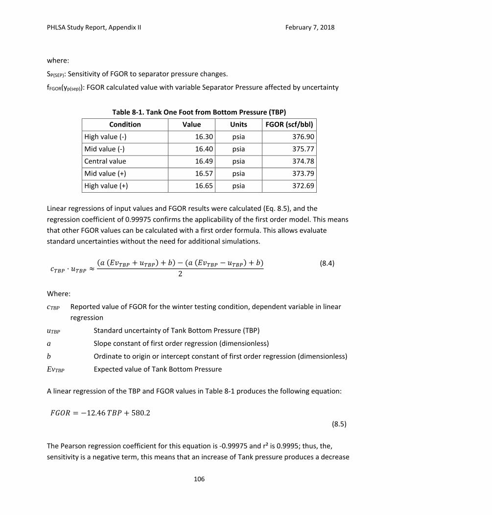
PHLSA Study Report, Appendix II February 7, 2018
106
where:
SP(SEP): Sensitivity of FGOR to separator pressure changes.
fFGOR(yp(sep)): FGOR calculated value with variable Separator Pressure affected by uncertainty
Table 8-1. Tank One Foot from Bottom Pressure (TBP)
Condition Value Units FGOR (scf/bbl)
High value (-) 16.30 psia 376.90
Mid value (-) 16.40 psia 375.77
Central value 16.49 psia 374.78
Mid value (+) 16.57 psia 373.79
High value (+) 16.65 psia 372.69
Linear regressions of input values and FGOR results were calculated (Eq. 8.5), and the
regression coefficient of 0.99975 confirms the applicability of the first order model. This means
that other FGOR values can be calculated with a first order formula. This allows evaluate
standard uncertainties without the need for additional simulations.
𝑐𝑇𝐵𝑃 · 𝑢𝑇𝐵𝑃 ≈(𝑎 (𝐸𝑣𝑇𝐵𝑃 + 𝑢𝑇𝐵𝑃) + 𝑏) − (𝑎 (𝐸𝑣𝑇𝐵𝑃 − 𝑢𝑇𝐵𝑃) + 𝑏)
2
(8.4)
Where:
cTBP Reported value of FGOR for the winter testing condition, dependent variable in linear
regression
uTBP Standard uncertainty of Tank Bottom Pressure (TBP)
a Slope constant of first order regression (dimensionless)
b Ordinate to origin or intercept constant of first order regression (dimensionless)
EvTBP Expected value of Tank Bottom Pressure
A linear regression of the TBP and FGOR values in Table 8-1 produces the following equation:
𝐹𝐺𝑂𝑅 = −12.46 𝑇𝐵𝑃 + 580.2
(8.5)
The Pearson regression coefficient for this equation is -0.99975 and r² is 0.9995; thus, the,
sensitivity is a negative term, this means that an increase of Tank pressure produces a decrease
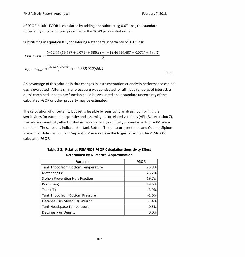
PHLSA Study Report, Appendix II February 7, 2018
107
of FGOR result. FGOR is calculated by adding and subtracting 0.071 psi, the standard
uncertainty of tank bottom pressure, to the 16.49 psia central value.
Substituting in Equation 8.1, considering a standard uncertainty of 0.071 psi:
𝑐𝑇𝐵𝑃 · 𝑢𝑇𝐵𝑃 ≈(−12.46 (16.487 + 0.071) + 580.2) − (−12.46 (16.487 − 0.071) + 580.2)
2
𝑐𝑇𝐵𝑃 · 𝑢𝑇𝐵𝑃 ≈(375.67−373.90)
2≈ −0.885 (SCF/BBL)
(8.6)
An advantage of this solution is that changes in instrumentation or analysis performance can be
easily evaluated. After a similar procedure was conducted for all input variables of interest, a
quasi-combined uncertainty function could be evaluated and a standard uncertainty of the
calculated FGOR or other property may be estimated.
The calculation of uncertainty budget is feasible by sensitivity analysis. Combining the
sensitivities for each input quantity and assuming uncorrelated variables (API 13.1 equation 7),
the relative sensitivity effects listed in Table 8-2 and graphically presented in Figure 8-1 were
obtained. These results indicate that tank Bottom Temperature, methane and Octane, Siphon
Prevention Hole Fraction, and Separator Pressure have the largest effect on the PSM/EOS
calculated FGOR.
Table 8-2. Relative PSM/EOS FGOR Calculation Sensitivity Effect
Determined by Numerical Approximation
Variable FGOR
Tank 1 foot from Bottom Temperature 26.8%
Methane/-C8 26.2%
Siphon Prevention Hole Fraction 19.7%
Psep (psia) 19.6%
Tsep (°F) -3.9%
Tank 1 foot from Bottom Pressure -2.0%
Decanes Plus Molecular Weight -1.4%
Tank Headspace Temperature 0.3%
Decanes Plus Density 0.0%
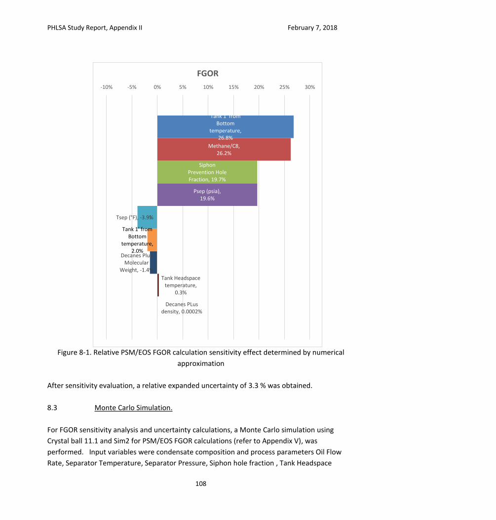
PHLSA Study Report, Appendix II February 7, 2018
108
Figure 8-1. Relative PSM/EOS FGOR calculation sensitivity effect determined by numerical
approximation
After sensitivity evaluation, a relative expanded uncertainty of 3.3 % was obtained.
8.3 Monte Carlo Simulation.
For FGOR sensitivity analysis and uncertainty calculations, a Monte Carlo simulation using
Crystal ball 11.1 and Sim2 for PSM/EOS FGOR calculations (refer to Appendix V), was
performed. Input variables were condensate composition and process parameters Oil Flow
Rate, Separator Temperature, Separator Pressure, Siphon hole fraction , Tank Headspace
Decanes PLus density, 0.0002%
Tank Headspace temperature,
0.3%
Decanes Plus Molecular
Weight, -1.4%
Tank 1' from Bottom
temperature, 2.0%
Tsep (°F), -3.9%
Psep (psia), 19.6%
Siphon Prevention Hole Fraction, 19.7%
Methane/C8, 26.2%
Tank 1' from Bottom
temperature, 26.8%
-10% -5% 0% 5% 10% 15% 20% 25% 30%
1
FGOR
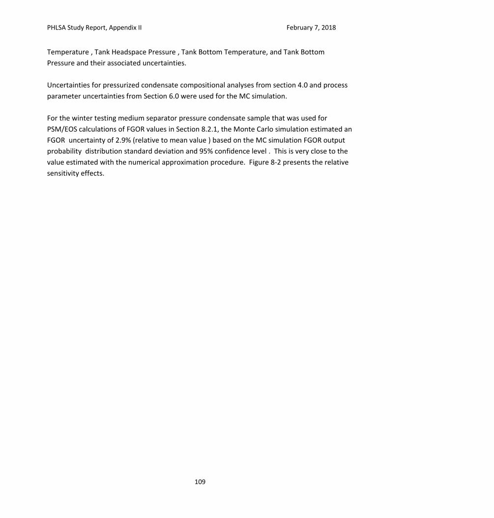
PHLSA Study Report, Appendix II February 7, 2018
109
Temperature , Tank Headspace Pressure , Tank Bottom Temperature, and Tank Bottom
Pressure and their associated uncertainties.
Uncertainties for pressurized condensate compositional analyses from section 4.0 and process
parameter uncertainties from Section 6.0 were used for the MC simulation.
For the winter testing medium separator pressure condensate sample that was used for
PSM/EOS calculations of FGOR values in Section 8.2.1, the Monte Carlo simulation estimated an
FGOR uncertainty of 2.9% (relative to mean value ) based on the MC simulation FGOR output
probability distribution standard deviation and 95% confidence level . This is very close to the
value estimated with the numerical approximation procedure. Figure 8-2 presents the relative
sensitivity effects.
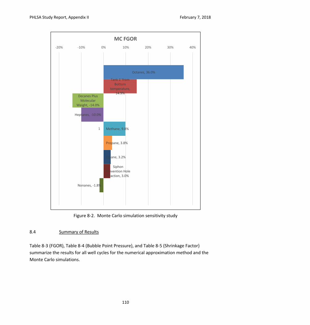
PHLSA Study Report, Appendix II February 7, 2018
110
Figure 8-2. Monte Carlo simulation sensitivity study
8.4 Summary of Results
Table 8-3 (FGOR), Table 8-4 (Bubble Point Pressure), and Table 8-5 (Shrinkage Factor)
summarize the results for all well cycles for the numerical approximation method and the
Monte Carlo simulations.
Nonanes, -1.8%
Siphon Prevention Hole Fraction, 3.0%
Ethane, 3.2%
Propane, 3.8%
Methane, 9.8%
Heptanes, -10.0%
Decanes Plus Molecular
Weight, -14.0%
Tank 1' from Bottom
temperature, 14.9%
Octanes, 36.0%
-20% -10% 0% 10% 20% 30% 40%
1
MC FGOR
PHLSA Study Report, Appendix II February 7, 2018
111
Table 8-3. Results of FGOR Uncertainty Calculations
Season Well Cycle
Sample
GPA 2103 Analysis GPA 2186 Analysis
Numerical
Approximation
Monte Carlo
Simulation
Numerical
Approximation
Monte Carlo
Simulation
SUMMER LP-3 3.8% 3.0% 4.0% 3.3%
SUMMER MP-3 2.8% 2.8% 3.1% 3.0%
SUMMER HP-3 2.8% 2.7% 3.7% 2.9%
WMULTI LP-1 4.9% 3.8% 4.7% 3.8%
WMULTI MP-2 3.8% 3.3% 3.7% 3.3%
WMULTI HP-1 3.3% 3.1% 3.0% 3.1%
Table 8-4. Results of Bubble Point Pressure Uncertainty Calculations
Season Well Cycle
Sample
GPA 2103 Analysis GPA 2186 Analysis
Numerical
Approximation
Monte Carlo
Simulation
Numerical
Approximation
Monte Carlo
Simulation
SUMMER LP-3 1.1% 2.2% 1.0% 2.9%
SUMMER MP-3 1.1% 2.2% 1.0% 2.9%
SUMMER HP-3 1.1% 2.2% 1.2% 2.9%
WMULTI LP-1 1.2% 3.0% 0.8% 3.0%
WMULTI MP-2 1.2% 3.0% 0.8% 3.0%
WMULTI HP-1 0.9% 3.1% 0.7% 3.1%
Table 8-5. Results of Shrinkage Factor Uncertainty Calculations
Season Well Cycle
Sample
GPA 2103 Analysis GPA 2186 Analysis
Numerical
Approximation
Monte Carlo
Simulation
Numerical
Approximation
Monte Carlo
Simulation
SUMMER LP-3 0.50% 0.44% 0.47% 0.44%
SUMMER MP-3 0.57% 0.50% 0.46% 0.49%
SUMMER HP-3 0.57% 0.57% 0.70% 0.54%
WMULTI LP-1 0.41% 0.32% 0.36% 0.32%
WMULTI MP-2 0.42% 0.38% 0.37% 0.38%
WMULTI HP-1 0.56% 0.55% 0.49% 0.55%
![الموقع الأول للدراسة في الجزائر · 2019-06-14 · NPb NPo ); 6˘ sh ˆ)6 ... 176 .gmol 1]˙ ˘ /!ˇ*6](https://img.pdfslide.net/doc/110x75/5f52686121ea2856d945d18b/-2019-06-14-npb-npo.jpg)


![based ionic liquids: OFET application and tribological ... · 3 [P22P113N][NTf2]4.3H2O (PzIL2a) 1 35-292 188 2.89 2.82 3H2O C39H73F25N13O23P3S8 2 292-454 371 87.78 1916.44 gmol-1](https://img.pdfslide.net/doc/110x75/5fdb557210743856e36f0850/based-ionic-liquids-ofet-application-and-tribological-3-p22p113nntf243h2o.jpg)