Embed Size (px)
Citation preview

PHOENICS-ESTER User Guide. CHAM Ref: CHAM/TR315
Document rev: 6
Doc. release date: 29 March 2019
Software version: PHOENICS 2019 v1.0
Responsible author: J C Ludwig
Other contributors: A Adam
Editor: J C Ludwig
Published by: CHAM
Confidentiality:
Classification: Unclassified
The copyright covers the exclusive rights to reproduction and distribution including reprints,
photographic reproductions, microform or any other reproductions of similar nature, and translations.
No part of this publication may be reproduced, stored in a retrieval system or transmitted in any form
or by any means, electronic, electrostatic, magnetic tape, mechanical, photocopying, recording or
otherwise, without permission in writing from the copyright holder.
© Copyright Concentration, Heat and Momentum Limited 2019
CHAM, Bakery House, 40 High Street, Wimbledon, London SW19 5AU, UK Telephone: 020 8947 7651 Fax: 020 8879 3497
E-mail: [email protected] Web site: http://www.cham.co.uk
PHOENICS – Your Gateway to CFD Success
Documentation for PHOENICS |TR 315

TR 315 PHOENICS-ESTER User Guide
2 PHOENICS-ESTER User Guide
CHAM – Your Gateway to CFD Success
PHOENICS-ESTER Reference Guide: TR 315
Table of Contents
1. Foreword 4
2. Introduction 5
3. ESTER Main menu 6
4. Geometry 7
4.1 Anode Settings 8
4.2 Electrical Connections to the Anodes 13
4.3 Cathode Settings 14
4.4 Electrical Connections to the Cathodes 15
5. Meshing 17
6. Properties 19
7. Models 20
8. Boundary Conditions 22
8.1 Cathode Conditions 22
8.2 Anode Conditions 23
8.3 Magnetic Fields 25
8.4 Other Settings 25
9. Numerics 26
10. ESTER-Specific Output 28
11. OBJECT Types Used by ESTER 30
11.1 Anode 30
11.2 Anode Stubs, Yokes, Rods, Bus- and Cross-bars 31
11.3 Cathode Blocks and Collector Bars 31
11.4 Freeze 32
11.5 Other Objects 32
12. Post Processing 33
12.1 Displaying the metal - electrolyte interface 33
12.2 Plotting vectors of current 34
12.3 Plotting vectors of other vector quantities 35
12.4 Creating Animations 35
12.5 Monitoring Rod Voltage and Current 35
12.6 Monitoring Collector-bar currents 36
12.7 Monitoring the Interface Height 36
13. Q1 Settings 37

TR 315 PHOENICS-ESTER User Guide
3 PHOENICS-ESTER User Guide
13.1 Domain Settings 37
13.2 Variables Passed to ESTRGR 39
13.3 Anode Object 41
13.4 Additional Monitoring flags 41
Appendix A. Mathematical Background 43
A.1 Some notes on the solution of the General Conservation Equation 43
A.2 Momentum Sources 43
A.3 The Potential Equation and Current Calculations 43
A.4 Potential Equation Sources 44
A.5 Magnetic Fields 46
Appendix B. Location of Anodes 47
Appendix C. Freeze 49
Appendix D. The Moving Grid and the Metal-Electrolyte Interface 50
Appendix E. ESTER File Formats 51
TR 315 PHOENICS-ESTER User Guide
4 PHOENICS-ESTER User Guide
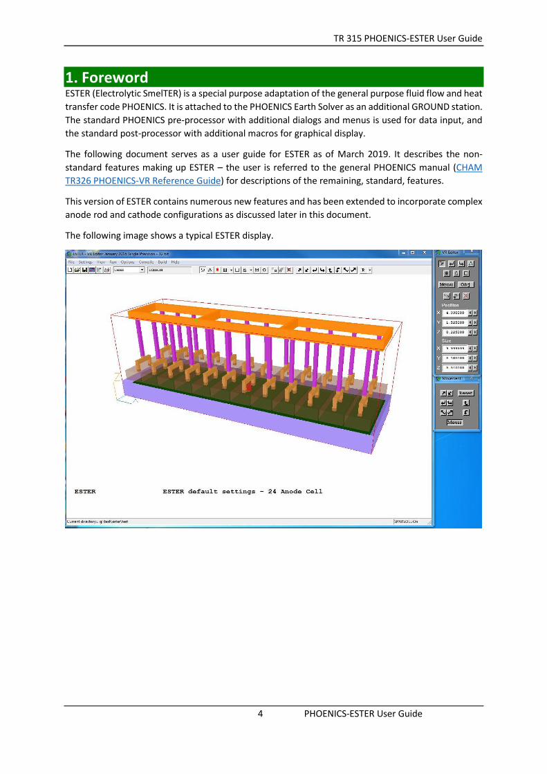
1. Foreword ESTER (Electrolytic SmelTER) is a special purpose adaptation of the general purpose fluid flow and heat
transfer code PHOENICS. It is attached to the PHOENICS Earth Solver as an additional GROUND station.
The standard PHOENICS pre-processor with additional dialogs and menus is used for data input, and
the standard post-processor with additional macros for graphical display.
The following document serves as a user guide for ESTER as of March 2019. It describes the non-
standard features making up ESTER – the user is referred to the general PHOENICS manual (CHAM
TR326 PHOENICS-VR Reference Guide) for descriptions of the remaining, standard, features.
This version of ESTER contains numerous new features and has been extended to incorporate complex
anode rod and cathode configurations as discussed later in this document.
The following image shows a typical ESTER display.

TR 315 PHOENICS-ESTER User Guide
5 PHOENICS-ESTER User Guide
2. Introduction ESTER solves for the steady state or transient fluid flow and electric potential distributions within an
aluminium reduction cell of the Hall Cell type that is found prevalently in industrial aluminium smelting.
The equations solved are pressure, P1, three velocity components U1, V1 and W1, and the electric
potential EPOT.
A primary feature of the Hall Cell is the presence of two distinct layers of fluid, which never intermingle.
The liquid metal is at the bottom, in contact with the cathode. The upper layer is the electrolyte, into
which the anodes are immersed. The height of the metal-electrolyte interface is adjusted periodically
to maintain hydrostatic equilibrium across the interface. The Lorentz forces driving the flow cause
pressure differences across the interface, which then deforms.
The enormous difference in conductivity between metal and electrolyte means that even small
changes in interface height can significantly alter the resistance paths, and hence current distributions.
This then feeds back to the Lorentz forces and the height distribution. (More mathematical and
technical details can be found in Appendix A to this document).
Whilst by default, ESTER solves only for the fluid behaviour and the electric potential, the two-phase
option of PHOENICS can also be activated to model the dispersion of gas bubbles from the anode
undersides, through the inter-anode and anode-wall gaps.
A schematic representation of the Hall type electrolysis cell is shown below:
The rest of this document discusses in some detail how to build the geometry illustrated above and
how to access and control all the model parameters relevant to an ESTER simulation. (We again remind
the reader to refer to the PHOENICS-VR Reference Guide (TR326) in order to clarify any general aspects
of PHOENICS with which they are unfamiliar).
Anode stubs and yoke
Steel collector bar
Cathode carbon
Liquid metal
Bath
Anode block
Anode rod
Copper insert
Freeze

TR 315 PHOENICS-ESTER User Guide
6 PHOENICS-ESTER User Guide
3. ESTER Main menu The controls for the anode and cathode configurations, and all other model paramaters are located on
the ESTER Main Menu. To display this menu, click the Menu icon on the tool bar, or the Menu
button on the hand-set. Either action will result in this dialog appearing:
The structure of these menus will be familiar to general PHOENICS users. The features unique to ESTER
are restricted to the top line of buttons – the Geometry / Properties / Models / Boundary and Numerics
panels. For descriptions of the Output, Initialisation and INFORM panels please refer to TR326,
PHOENICS-VR Reference Guide.
The functions of the ESTER-specific panels are as follows:
Geometry – sets the size of the reduction cell, the anode and cathode configurations and can
control the meshing.
Properties – sets the density and laminar kinematic viscosity of the metal and electrolyte, and
the electrical conductivities of the materials used in the construction of the cell.
Models – controls whether the potential equation is solved, and which terms are included in
the interface-height adjustment sequence.
Boundary – sets the cell current and voltage, the voltages at the anode rods, the currents at
the busbar and collector bars, and the magnetic field initialisation.
Numerics – sets the numerical controls for the solution.
Output – sets ESTER-specific output controls.
Each of these panels will now be described in detail.

TR 315 PHOENICS-ESTER User Guide
7 PHOENICS-ESTER User Guide
4. Geometry The fundamental geometry of the electrolysis cell to be modelled is governed by the ‘Geometry’ tab.
Clicking this button brings up the following dialog box:
Time dependence: when set to Steady the calculation is steady-state.
When set to Transient, the calculation is transient, and the iterative solution procedure will be
repeated at each time step. The number of steps to perform and the time step size is set from
the Time step settings dialog.
Include anodes: when set to Yes, the anodes, and at the user’s choice the stubs, yokes, rods
and busbars are included in the model. When set to No, the anodes are not included at all, and
the solution domain ends at the upper surface of the electrolyte layer.
Include cathode blocks: when set to Yes, the cathode blocks, and at the user’s choice the
collector bars, are included in the model. When set to No, the solution domain starts at the
upper surface of the cathode blocks.
Depth of metal layer: sets the depth of the metal layer above the cathode blocks.
Depth of electrolyte bath: sets the total depth of the electrolyte bath.
The overall dimensions of the model are displayed at the bottom of this panel (but note this is
not user input but calculated internally).
Anode Settings: This button is only shown if the anodes are to be included. It displays the
anode settings panel which allows the user to select anode properties such as their dimensions
and number, together with whether stubs, cross-bars, busbars, tapping gaps and connectors
are present or not. The dimensions of these objects are also set here together with other
variables such as the inter-anode spacing, anode to cathode distance and freeze block
inclusion. (See 4.1 Anode Settings below for more detail).
Cathode Settings: This button is only shown if the cathode blocks are to be included. It displays
the cathode setting panel where the user can control the cathode block dimensions together
with whether collector bars are to be included and, if so, their geometry. The user may also
add electrical contacts in the form of copper and cast iron inserts to the collector bars. Finally,

TR 315 PHOENICS-ESTER User Guide
8 PHOENICS-ESTER User Guide
there is also the option to import CAD geometry if an alternative cathode geometry (rather
than the default cuboid type) is desired. (See 4.3 Cathode Settings below for more detail).
Meshing: If automatic meshing is toggled ON, the user has the option to click the ‘meshing’
button. This displays the ESTER automatic meshing dialog box where the user can specify the
number of cells in key regions in the electrolysis cell. NOTE: If automatic meshing is turned
off, users can control the grid manually. (See 5 Meshing below for more detail.)
4.1 Anode Settings Selecting ‘Anode settings’ displays the following dialog box (where, in this case, everything has been
toggled as ‘On’):
Number of anodes: sets the number of anodes in the X and Y directions. (Note: there can be
only a single layer of anodes in the z direction).
Anode size: sets the physical size of the anodes in the X, Y and Z directions.
Include tapping gap(s): A tapping gap represents a physical space between anodes where metal
is siphoned out of the cell. Geometrically, it appears as a spacing that is larger than the regular
inter-anode gap. The user can choose to include such gaps if desired.
Tapping gap in direction: controls whether the tapping gap(s) are in the X or Y direction.
Number of gaps: If activated, there can be one or two tapping gaps.
Gap size: is the size of each tapping gap.
Gap after anode: this entry places the gap(s) after the anode number(s) selected. Anode 1 is the
left-most.
The effect of activating the tapping gap is shown in the figure below, where two gaps are set in
X, after the sixth and seventh anodes.

TR 315 PHOENICS-ESTER User Guide
9 PHOENICS-ESTER User Guide
Example of two tapping gaps (of 0.8m each) in the x direction after anode numbers 6 & 7.
Regular inter-anode gap: controls the regular spacing in X and Y between each of the anode
blocks.
Anode to wall distance: controls the size of the gap between the left or right edge of the domain
and the start and end of the adjacent anode blocks. The gaps are equal at both ends and can be
set separately in X and Y.
Anode to cathode distance (ACD): controls the vertical (Z) distance from the base of the anode
block to the top of the metal layer beneath the electrolyte solution. (Note: Following standard
convention, this does NOT in fact measure the physical distance from anode to cathode).
Anode/stub yoke configuration: this button displays the following drop-down menu:
From here the user can select whether anode rods, yokes and stubs are to be included in the
model. Note that rods, yokes and stubs are all coupled – one cannot have a rod without stubs
and yokes.
If ‘None’ is chosen, the solution domain ends at the upper surface of the anode blocks. If one of
the other configurations is chosen, then the stubs, yokes and rods will be included in the model.
The m*n nomenclature refers to the number of stubs in X and Y respectively. The 1*2 – 2*2
configurations apply to a single anode, each fed by a single rod. The 2*2 and 2*4 configurations
apply to pairs of adjacent (in X) anodes. These are joined by the yoke and are fed by a single rod
per pair.
The next table shows the available configurations.

TR 315 PHOENICS-ESTER User Guide
10 PHOENICS-ESTER User Guide
1 * 2 1 * 3 1 * 4
2 * 2 2 * 3 2 * 4
Anode stub diameter: the diameter of the anode stubs (in the model the stubs are treated as
square with the equivalent area).
Depth of stub in anode: the depth to which the stub is embedded in the anode block.
Anode yoke distance (top to top): the distance from the top of the anode block to the top of
the yoke.
Anode yoke dimensions: the dimensions of the yoke in X, Y and Z.
Anode rod dimensions: the dimensions of the anode rod in X, Y and Z.
Yoke to anode rod steel connector: the height of the steel connector between the yoke and the
bottom of the anode rod, as shown below:
Include cast-iron layer: when set to Yes, the cast iron layer surrounding the tips of the anode
stubs immersed within the anode itself is included, to act as electrical contact layer. If toggled
on, the user can then specify the thickness of this layer.
Note that this layer is treated as a sub-grid element, and does not need to be explicitly meshed.
Include bus and cross-bars: incorporates electrical overhead rails into the model.
Steel connector
TR 315 PHOENICS-ESTER User Guide
11 PHOENICS-ESTER User Guide
Busbar dimensions: sets the dimensions of the busbars in X, Y and Z. The busbars are assumed
to lie along the anode-rod centre lines in the Y direction. In the X direction they are located
centrally in the cell, and in Z they sit on the top of the anode rods.
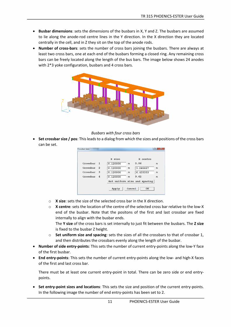
Number of cross-bars: sets the number of cross bars joining the busbars. There are always at
least two cross bars, one at each end of the busbars forming a closed ring. Any remaining cross
bars can be freely located along the length of the bus bars. The image below shows 24 anodes
with 2*3 yoke configuration, busbars and 4 cross bars.
Busbars with four cross bars
Set crossbar size / pos: This leads to a dialog from which the sizes and positions of the cross bars
can be set.
o X size: sets the size of the selected cross bar in the X direction.
o X centre: sets the location of the centre of the selected cross bar relative to the low-X
end of the busbar. Note that the positons of the first and last crossbar are fixed
internally to align with the busbar ends.
The Y size of the cross bars is set internally to just fit between the busbars. The Z size
is fixed to the busbar Z height.
o Set uniform size and spacing: sets the sizes of all the crossbars to that of crossbar 1,
and then distributes the crossbars evenly along the length of the busbar.
Number of side entry-points: This sets the number of current entry-points along the low-Y face
of the first busbar.
End entry-points: This sets the number of current entry-points along the low- and high-X faces
of the first and last cross bar.
There must be at least one current entry-point in total. There can be zero side or end entry-
points.
Set entry-point sizes and locations: This sets the size and position of the current entry-points.
In the following image the number of end entry-points has been set to 2.
TR 315 PHOENICS-ESTER User Guide
12 PHOENICS-ESTER User Guide
o X / Y size: This sets the X (for side entries) or Y (for end entries) size of the current
entry-point. The sizes are trapped relative to the centre location such that the entry
point does not extend beyond either end of the busbar.
o X / Y centre: This sets the X or Y location of the centre of the current entry-point
relative to the start of the busbar. For side entries this is the low-X end, for end entries
it is the low-Y face. The locations are trapped relative to the size such that the entry
point does not extend beyond either end of the busbar.
o Far end: When not ticked, the end entry-point is on the low-X face of the first cross
bar. When ticked, it is on the high-X face of the last cross bar.
The Z size is fixed to the busbar Z height.
o Set uniform size and spacing: sets the sizes of all the entry-points to that of entry-
point 1, and then distributes the entry-points evenly along the length of the busbar (in
X), or length of crossbar plus twice the busbar width (in Y).
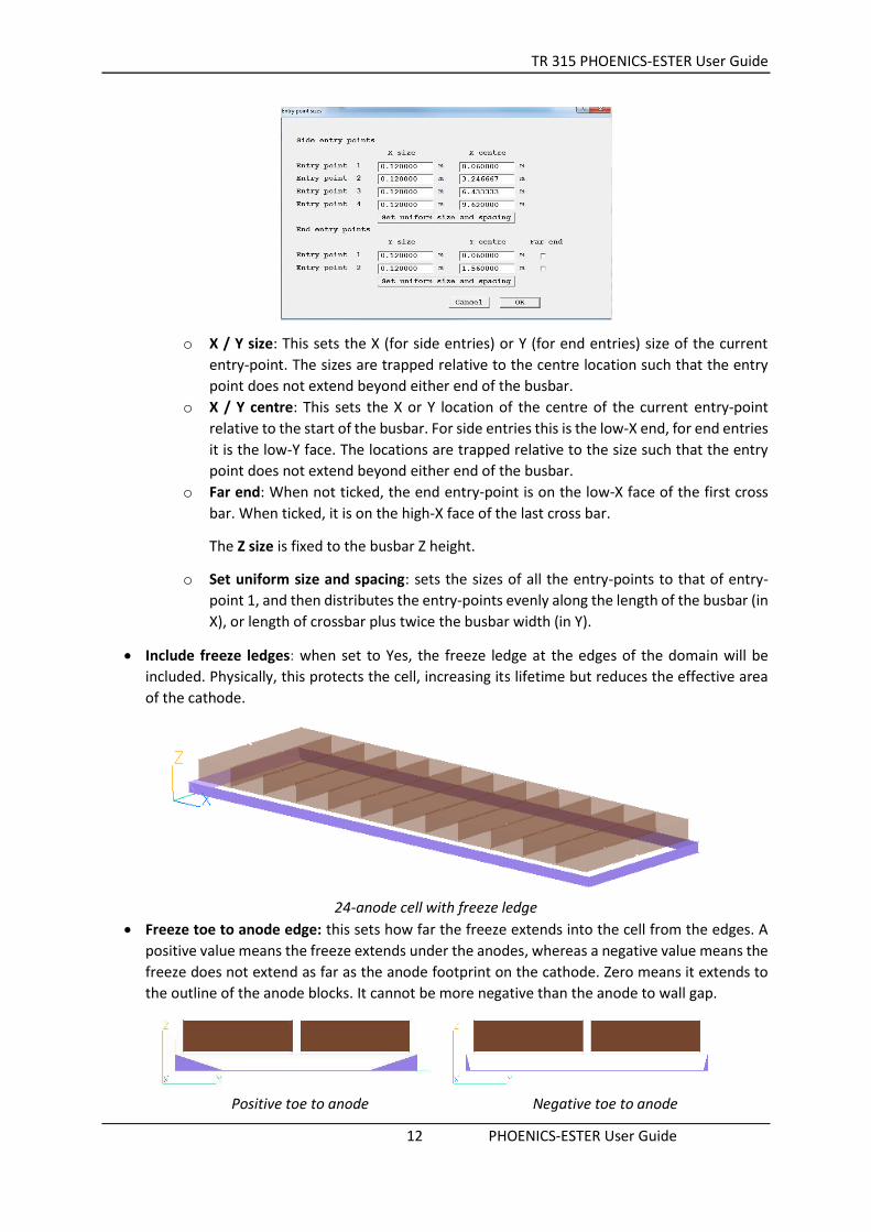
Include freeze ledges: when set to Yes, the freeze ledge at the edges of the domain will be
included. Physically, this protects the cell, increasing its lifetime but reduces the effective area
of the cathode.
24-anode cell with freeze ledge
Freeze toe to anode edge: this sets how far the freeze extends into the cell from the edges. A
positive value means the freeze extends under the anodes, whereas a negative value means the
freeze does not extend as far as the anode footprint on the cathode. Zero means it extends to
the outline of the anode blocks. It cannot be more negative than the anode to wall gap.
Positive toe to anode Negative toe to anode

TR 315 PHOENICS-ESTER User Guide
13 PHOENICS-ESTER User Guide
4.2 Electrical Connections to the Anodes If the anode stubs and rods are not included, a single fixed potential condition is applied at the upper
Z face of the solution domain. The program determines which cells lie inside an anode block, and
applies the fixed voltage at those locations. The voltage can either be a fixed constant value, or a cell-
by-cell distribution can be set by modifying the ESTRGR subroutine.
If the anode stubs and yokes are included, but the busbars are not, a fixed voltage condition is applied
at the top of each anode rod. The potential at each rod is set on the Boundary panel – Section 8. The
voltage locations are blue in the following image. One is circled in red.
Fixed-voltage locations (blue) for 24-anode cell with 2*3 yoke
If the busbars are also included, then a fixed current condition is applied at each current entry-point
and a fixed voltage is applied at the mid-point of the left-most cross bar. The current entry-points are
green and the fixed voltage point is blue in the following image. The numbers, sizes and locations of
the current entry-points and the cross bars can be different.
Fixed-current (green) and fixed-voltage (blue) locations on busbar
The actual values of the currents and anode potential are set in the Boundary panel – Section 8.

TR 315 PHOENICS-ESTER User Guide
14 PHOENICS-ESTER User Guide
4.3 Cathode Settings Selecting ‘Cathode settings’ brings up the following dialog box (all options are turned on)
:
Number of cathode blocks: sets the number of cathode blocks in the X direction. It is assumed
there is always one block in the Y direction.
Cathode dimensions: sets the dimensions of the cathode blocks in X, Y and Z. The size * number
in X and Y cannot exceed the overall cell size, which is determined by the number and size of
anodes and inter-anode gaps. If the total size of the cathode carbon panel is less than the cell
size, the free space at the edges is filled with an insulating material.
Default cathode geometry: sets the name of the geometry file to be used when creating the
cathode blocks. ‘default’ is a rectangular block, so will give a flat cathode upper surface. A
different shape can be imported as a CAD file. This will then be used for all the cathode blocks.
Default flat cathodes Shaped cathodes
The shape of each cathode block can also be set individually from the ‘Shape’ tab of the Object
Specification dialog for an individual cathode by importing the geometry as a CAD file.
More information about importing CAD files is given in TR326, PHOENICS-VR Reference Guide.
Include collector bars: when set to Yes, the collector bars at the bottom of the cathode blocks
are included in the model.
Number of collector bars/block: sets the number of collector bars in X in each cathode block.Up
to 3 collector bars per block are allowed as long as they will fit within the width of a cathode
block. In the Y direction it is assumed that the bars extend to the edges of the cell. The number
of bars is thus one if the centre gap is zero, or two if the centre gap is finite.
Collector bar dimensions: sets the dimensions of the collector bars in the X, Y and Z directions.
The number of bars per cathode block times the X size cannot exceed the X size of a cathode
block. If twice the Y size plus the collector bar centre gap exceeds the bath width, the edges of
the domain outboard the bath are filled with a non-conducting solid.
Collector bar centre gap: If the centre gap is set to zero, then a single collector bar is placed
parallel to the y-axis. If the gap is non-zero, then there are two separate collector bars parallel
to the y-axis separated by this gap size. (Note: In order to refresh the dialog box on changing

TR 315 PHOENICS-ESTER User Guide
15 PHOENICS-ESTER User Guide
the centre gap in order to update the number of collector bars in the y-direction, the user
should press the ‘Apply’ button.
The following image shows 14 cathode blocks, each with 2 collector bars giving a total of 28
collector bars in X. The centre gap is non-zero, so there are 2 bars in Y.
Two collector bars per cathode block, finite centre gap and filled edge gaps
Include copper inserts: includes a copper insert inside the collector bar itself. It is located
centrally immediately under the upper face of the collector bar.
Copper insert dimensions: sets the X, Y and Z sizes of the copper insert. These may not be
bigger than the collector bar itself.
Offset from domain edge: sets the distance between the edge of the domain (and hence
collector bar) and the start of the copper insert.
Include cast iron inserts: includes a thin cast-iron layer around the outside of each collector
bar.
Cast iron insert dimensions: sets the thickness of the cast iron layer. Note that this layer is
treated as a sub-grid element, and does not need to be explicitly meshed. The image below
shows the cast-iron inserts and copper inserts.
Cast-iron and copper inserts
4.4 Electrical Connections to the Cathodes If the cathode blocks are not included, or if they are included but the collector bars are not, a single
fixed-current condition is applied at the base of the solution domain. The current density can be a
single fixed value, or a cell-by-cell distribution can be read from a file.
If the cathode blocks and collector bars are included, a fixed current extraction condition is applied at
the ends of each collector bar The following image shows the current-condition locations in red.

TR 315 PHOENICS-ESTER User Guide
16 PHOENICS-ESTER User Guide
The current exit condition includes the copper inserts, if they are present.
The actual values of the cell current or the collector bar currents are set in the Boundary panel – Section
8.

TR 315 PHOENICS-ESTER User Guide
17 PHOENICS-ESTER User Guide
5. Meshing Selecting ‘Meshing’ displays the following dialog box
If the automatic meshing option is set to ON, the user has access to the above dialogue box which
allows the number of cells/slabs in important regions to be set. (A slab is a layer of cells in the Z-
direction). The selected number of cells in the X- and Y-directions as well as slabs in the Z-direction
will then be distributed as evenly as possible within the selected part of the domain.
The items which cause the grid to align with their edges are:
o The anodes in all three directions
o The top of the steel yoke-rod connector in Z
o The top of the anode rod in Z
o The upper surface of the electrolyte bath
o The metal-electrolyte interface in Z
o The top of the cathode blocks in Z
o The collector bars in Z
o The copper inserts in Z.
The ESTER auto-meshing dialog allows the number of cells in each of these zones to be set. The
yokes, rods, bus- and cross-bars, cathode blocks , collector bars and copper inserts do not force the
X and Y grid to align with their edges. Provided there is a reasonable number of cells, they will be
detected correctly.The cast-iron inserts in the anodes and cathodes are always treated as sub-grid
items.
If ESTER automatic meshing is OFF, all items (other than the cast iron inserts) cause the grid to align
with their edges in all three directions. The standard PHOENICS auto-meshing will be turned on in
X and Y.
In Z, the standard auto-mesh will be initially turned on, but the once the grid has been built around
the geometry the Z-direction grid will be reset to manual and the number of Z planes in the bath
under the anodes will be reset to that set in the ESTER dialog.
Any further changes then made by the user via the PHOENICS environment will be retained. To
access the meshing dialog, click the icon on the menu bar or hand-set then click on the grid. The
number of cells per grid region can now be set.

TR 315 PHOENICS-ESTER User Guide
18 PHOENICS-ESTER User Guide
A file called ‘grid.txt’ containing the cell face locations in each coordinate direction is written whenever
‘File – Save working files’ or ‘Run – Solver’ is clicked. The format of this file is given in the Appendix.
TR 315 PHOENICS-ESTER User Guide
19 PHOENICS-ESTER User Guide
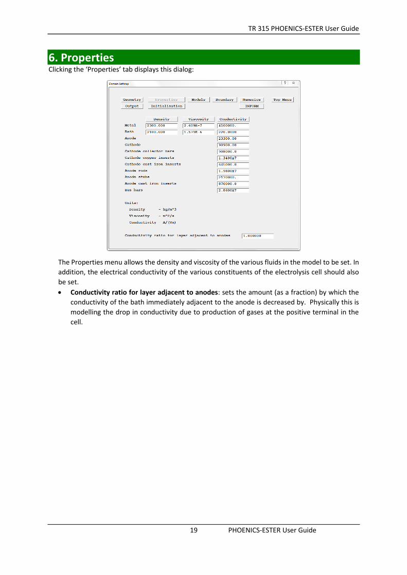
6. Properties Clicking the ‘Properties’ tab displays this dialog:
The Properties menu allows the density and viscosity of the various fluids in the model to be set. In
addition, the electrical conductivity of the various constituents of the electrolysis cell should also
be set.
Conductivity ratio for layer adjacent to anodes: sets the amount (as a fraction) by which the
conductivity of the bath immediately adjacent to the anode is decreased by. Physically this is
modelling the drop in conductivity due to production of gases at the positive terminal in the
cell.
TR 315 PHOENICS-ESTER User Guide
20 PHOENICS-ESTER User Guide
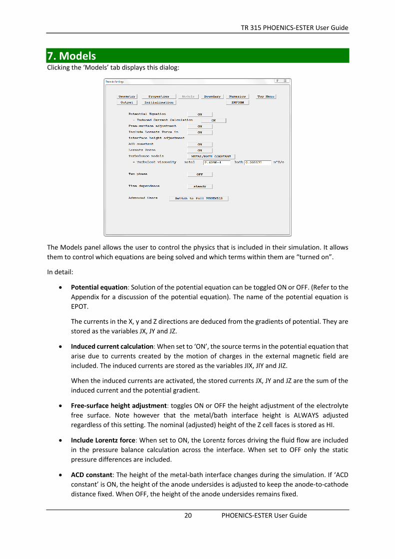
7. Models Clicking the ‘Models’ tab displays this dialog:
The Models panel allows the user to control the physics that is included in their simulation. It allows
them to control which equations are being solved and which terms within them are “turned on”.
In detail:
Potential equation: Solution of the potential equation can be toggled ON or OFF. (Refer to the
Appendix for a discussion of the potential equation). The name of the potential equation is
EPOT.
The currents in the X, y and Z directions are deduced from the gradients of potential. They are
stored as the variables JX, JY and JZ.
Induced current calculation: When set to ‘ON’, the source terms in the potential equation that
arise due to currents created by the motion of charges in the external magnetic field are
included. The induced currents are stored as the variables JIX, JIY and JIZ.
When the induced currents are activated, the stored currents JX, JY and JZ are the sum of the
induced current and the potential gradient.
Free-surface height adjustment: toggles ON or OFF the height adjustment of the electrolyte
free surface. Note however that the metal/bath interface height is ALWAYS adjusted
regardless of this setting. The nominal (adjusted) height of the Z cell faces is stored as HI.
Include Lorentz force: When set to ON, the Lorentz forces driving the fluid flow are included
in the pressure balance calculation across the interface. When set to OFF only the static
pressure differences are included.
ACD constant: The height of the metal-bath interface changes during the simulation. If ‘ACD
constant’ is ON, the height of the anode undersides is adjusted to keep the anode-to-cathode
distance fixed. When OFF, the height of the anode undersides remains fixed.

TR 315 PHOENICS-ESTER User Guide
21 PHOENICS-ESTER User Guide
Lorentz force: The Lorentz force arises from the movement of charge through a magnetic field,
and it drives the fluid flow in the electrolyte / metal bath. The effect of these forces can be
included by toggling Lorentz force ON. By toggling this OFF, the effect of the Lorentz force on
the fluid motion is not included. The three components of the Lorentz force are stored as FX,
FY and FZ.
Turbulence models: allows the user to select a turbulence model as best suits their
application: The options are:
o Single constant effective turbulent kinematic viscosity for metal and bath zones. (The
user may input their desired value in m2/s).
o Different constant effective turbulent kinematic viscosities for metal and bath zones.
(The user may again input their desired values in m2/s).
o Any of the standard PHOENICS turbulence models.
Two phase: The PHOENICS two-phase capability may be toggled here. This allows modelling
of the gas phase that is produced at the anodes. If this is toggled ON, an extra set of equations
is solved for the velocity of the gas and its distribution.
Time dependence: switches between steady-state and transient operation. When set to
Unsteady, the extra ‘Set/Modify time steps’ button leads to a panel where the duration of the
transient and the number of time steps can be set.
Switch to full PHOENICS: is included if some additional functionality is needed that falls
outside of the options available within the ESTER GUI (such as the solution for energy
equations e.g. temperature, enthalpy).

TR 315 PHOENICS-ESTER User Guide
22 PHOENICS-ESTER User Guide
8. Boundary Conditions Clicking the ‘Boundary’ tab displays this dialog, shown here in its simplest form:
The boundary conditions panel takes one of several forms, depending on whether the collector bars
or anode rods or anode busbars are included or not. If there are no collector bars and the anode
rod/stub/yoke configuration is ‘None’, the panel is as shown above.
8.1 Cathode Conditions Cathode current distribution: This sets the current distribution at the base of the solution
domain. This will be the bottom of the cathode blocks if they are included, or the upper surface
of the cathode blocks if they are not. The current density in A/m2 can either be a constant, or
a cell-by-cell value can be read from a file. The format of the file is described in the Appendix.
If the cathode collector bars are included the cathode current setting section changes to this:
Set collector bar currents: This leads to a dialog from which the current at each end of each
collector bar can be set. It is shown below. The remainder of the panel does not change.

TR 315 PHOENICS-ESTER User Guide
23 PHOENICS-ESTER User Guide
o Set total cell current: This sets the target total current through the cell in Amps.
o Bar 1 End 1 End 2: These and subsequent input boxes set the current at each end of
each collector bar. If there are too many bars to fit on the dialog extra buttons appear
which allow the list of collector bars to be scrolled up and down.
o Actual total cell current: This displays the actual total current – it is not an input box.
It is the sum of all the collector bar currents. Clicking any ‘Apply’ button will update
this value using the latest currents.
o Set all currents to default: This will reset the current at each end of each collector bar
to the target cell current divided by the total number of bar ends. This value is shown
in brackets on the button. It will be updated if ‘Apply’ is clicked after entering a new
target current.
o Adjust currents to sum to set current: This will adjust each current by the ratio of the
target total current to the actual total current. The effect is to achieve the target
current whilst retaining the relative distribution amongst the bar ends.
If the anode busbars are included, and the total cell current on exit from the dialog is
different from that on entry, the opportunity is offered to adjust the busbar currents so
that they sum to the new total cell current.
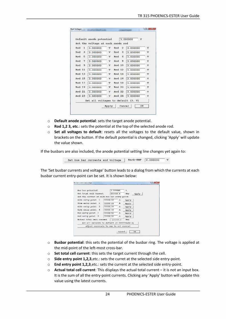
8.2 Anode Conditions Anode potential: sets the voltage applied at the anodes. If the yokes and rods are not included,
the voltage is applied at the upper face of the anode blocks. If they are included, but the
busbars are not, the voltage is applied at the top of each anode rod. The input box changes to
this button:
The ‘Set anode rod potentials’ button leads to a dialog from which the voltages at each anode
rod can be set. It is shown below:
TR 315 PHOENICS-ESTER User Guide
24 PHOENICS-ESTER User Guide
o Default anode potential: sets the target anode potential.
o Rod 1,2 3, etc.: sets the potential at the top of the selected anode rod.
o Set all voltages to default: resets all the voltages to the default value, shown in
brackets on the button. If the default potential is changed, clicking ‘Apply’ will update
the value shown.
If the busbars are also included, the anode potential setting line changes yet again to:
The ‘Set busbar currents and voltage’ button leads to a dialog from which the currents at each
busbar current entry-point can be set. It is shown below:
o Busbar potential: this sets the potential of the busbar ring. The voltage is applied at
the mid-point of the left-most cross-bar.
o Set total cell current: this sets the target current through the cell.
o Side entry point 1,2,3,etc.: sets the curret at the selected side entry-point.
o End entry point 1,2,3,etc.: sets the current at the selected side entry-point.
o Actual total cell current: This displays the actual total current – it is not an input box.
It is the sum of all the entry-point currents. Clicking any ‘Apply’ button will update this
value using the latest currents.

TR 315 PHOENICS-ESTER User Guide
25 PHOENICS-ESTER User Guide
o Set all currents to default: This will reset the current at each entry-point to the target
cell current divided by the total number of entry-ponts. This value is shown in brackets
on the button. It will be updated if ‘Apply’ is clicked after entering a new target current.
o Adjust currents to sum to set current: This will adjust each current by the ratio of the
target total current to the actual total current. The effect is to achieve the target
current whilst retaining the relative distribution amongst the entry-points.
If the collector bars are included, and the total cell current on exit from the dialog is
different from that on entry, the opportunity is offered to adjust the collector bar currents
so that they sum to the new total cell current.
If the collector bars are not included, then on exit the cathode current density is adjusted
to the sum of the bus currents divided by the area of the cathode blocks
Back EMF: introduces a potential drop across the anode bath-interface.
8.3 Magnetic Fields Initial magnetic field: ESTER does not calculate the magnetic field, so values must be supplied.
The field can be expressed analytically as a polynomial or linear form, in which case the user
specifies the necessary coefficients. (The expansion parameters X, Y are measured from the
centre of the cell). Alternatively the magnetic field can be read in from a file. The file format is
given in the Appendix. The three components of the magnetic field are stored as BX, BY and
BZ.
8.4 Other Settings Units: ESTER expects the magnetic field to be specified in Tesla. The user-specified field can be
in Gauss, Tesla or MilliTesla. The BX, BY and BZ fields seen in the post-processor or in the
RESULT file will have been converted to Tesla.
Initial interface height: the height of the metal-electrolyte interface at the start of the
calculation can be set in this panel. The options are:
o flat,
o constant gradient in x,
o constant gradient in y or
o read from a file. The format of the file is given in the Appendix
For the constant-gradient options, additional input boxes appear for the displacement at each
end of the cell.
Initial anode heights: the initial heights of the anode undersides can either be flat, or read
from a file. The format of the file is given in the Appendix.
It should be noted that all the options relating to ‘read from a file’ are completely dependent on the
number of data entries in the file exactly matching the number of computational cells on an X-Y plane.
If the grid is changed, any such files will have to be updated to fit the new grid.
A file called ‘grid.txt’ containing the cell face locations in each coordinate direction is written whenever
‘File – Save working files’ or ‘Run – Solver’ is clicked. The format of this file is given in the Appendix.
TR 315 PHOENICS-ESTER User Guide
26 PHOENICS-ESTER User Guide
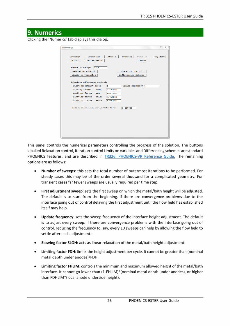
9. Numerics Clicking the ‘Numerics’ tab displays this dialog:
This panel controls the numerical parameters controlling the progress of the solution. The buttons
laballed Relaxation control, Iteration control Limits on variables and Differencing schemes are standard
PHOENICS features, and are described in TR326, PHOENICS-VR Reference Guide. The remaining
options are as follows:
Number of sweeps: this sets the total number of outermost iterations to be performed. For
steady cases this may be of the order several thousand for a complicated geometry. For
transient cases far fewer sweeps are usually required per time step.
First adjustment sweep: sets the first sweep on which the metal/bath height will be adjusted.
The default is to start from the beginning. If there are convergence problems due to the
interface going out of control delaying the first adjustment until the flow field has established
itself may help.
Update frequency: sets the sweep frequency of the interface height adjustment. The default
is to adjust every sweep. If there are convergence problems with the interface going out of
control, reducing the frequency to, say, every 10 sweeps can help by allowing the flow field to
settle after each adjustment.
Slowing factor SLOH: acts as linear relaxation of the metal/bath height adjustment.
Limiting factor FDH: limits the height adjustment per cycle. It cannot be greater than (nominal
metal depth under anodes)/FDH.
Limiting factor FHLIM: controls the minimum and maximum allowed height of the metal/bath
interface. It cannot go lower than (1-FHLIM)*(nominal metal depth under anodes), or higher
than FDHLIM*(local anode underside height).

TR 315 PHOENICS-ESTER User Guide
27 PHOENICS-ESTER User Guide
Limiting factor FRCON: acts to slow down the rate of change of the height of the metal bath
interface. (Values >1.0 slow it down).
Linear relaxation for Lorentz force: applies a linear relaxation factor to the sweep-to-sweep
change in Lorentz force.
TR 315 PHOENICS-ESTER User Guide
28 PHOENICS-ESTER User Guide
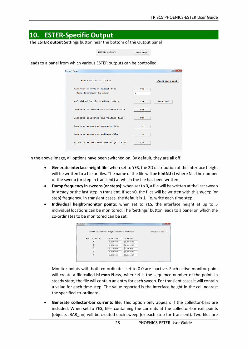
10. ESTER-Specific Output The ESTER output Settings button near the bottom of the Output panel
leads to a panel from which various ESTER outputs can be controlled.
In the above image, all options have been switched on. By default, they are all off.
Generate interface height file: when set to YES, the 2D distribution of the interface height
will be written to a file or files. The name of the file will be hintN.txt where N is the number
of the sweep (or step in transient) at which the file has been written.
Dump frequency in sweeps (or steps): when set to 0, a file will be written at the last sweep
in steady or the last step in transient. If set >0, the files will be written with this sweep (or
step) frequency. In transient cases, the default is 1, i.e. write each time step.
Individual height-monitor points: when set to YES, the interface height at up to 5
individual locations can be monitored. The ‘Settings’ button leads to a panel on which the
co-ordinates to be monitored can be set:
Monitor points with both co-ordinates set to 0.0 are inactive. Each active monitor point
will create a file called hi-mon-N.csv, where N is the sequence number of the point. In
steady state, the file will contain an entry for each sweep. For transient cases it will contain
a value for each time-step. The value reported is the interface height in the cell nearest
the specified co-ordinate.
Generate collector-bar currents file: This option only appears if the collector-bars are
included. When set to YES, files containing the currents at the collector-bar exit points
(objects JBAR_nn) will be created each sweep (or each step for transient). Two files are

TR 315 PHOENICS-ESTER User Guide
29 PHOENICS-ESTER User Guide
created, cbars_1.csv containing the currents at the low-Y ends of the collector-bars
(JBAR_0001, JBAR_0003 etc), and cbars_2.csv containing the currents at the high-Y ends
(JBAR_0002, JBAR_0004 etc). The values are the total currents in Amps.
Generate anode-rod currents file: This option only appears if anodes are active. When set
to YES, files containing the currents at the upper ends of the anode rods (objects VTAB_nn)
will be created each sweep (or each step for transient). Two files are created, rods_j_1.csv
containing the currents in the low-Y anode rods (VTAB_0001, VTAB_0003 etc) and
rods_j_2.csv containing the currents in the high-Y rods (VTAB-0002, VTAB_0004 etc). The
values are the currents in Amps/m2 in a cell located nearest the centreline of each rod.
Generate anode-rod voltage file: This option only appears if anodes are active. When set
to YES, files containing the voltage at the upper ends of the anode rods (objects VTAB_nn)
will be created each sweep (or each step for transient). Two files are created, rods_v_1.csv
containing the voltage in the low-Y anode rods (VTAB_0001, VTAB_0003 etc) and
rods_v_2.csv containing the voltage in the high-Y rods (VTAB-0002, VTAB_0004 etc). The
values are the voltage in Volts in a cell located nearest the centreline of each rod.
Store relative interface height (HINT): This creates an additional 3D stored variable
named HINT which is filled with the distance the interface has moved from it’s nominal,
flat, position:
HINT = current interface height – nominal interface height
Although it is stored as a 3D variable, HINT is actually the same at each Z location.

TR 315 PHOENICS-ESTER User Guide
30 PHOENICS-ESTER User Guide
11. OBJECT Types Used by ESTER There is only one object type which is specific to ESTER. This is the ANODE type. All the other elements
of the Hall Cell are composed of standard PHOENICS object types. The components of the cell are
automatically created from the following objects.
11.1 Anode Each anode is made using an ANODE type object. The attributes of the ANODE type can be seen by
double-clicking an anode on the screen, or in the Object Management Dialog, and then clicking the
‘Attributes’ button:
Each individual anode can be de-activated by changing ‘Anode is active Yes’ to ‘No’. In that case, the
anode remains in the model but the material is changed from the normal anode carbon to an insulating
material.
Each anode can also be raised from its nominal position.
Raised in-active anode
When active, the anode material is set to material number 100. The electrical conductivity of the anode
material is set on the Properties panel’, Chapter 6. Inactive anodes are set to material 198.
By default, the anodes are rectangular blocks. It is possible to assign other shapes to the individual
anodes by opening the Object Specification Dialog for an anode object and then importing a different
geometry from the ‘Shape’ tab.
TR 315 PHOENICS-ESTER User Guide
31 PHOENICS-ESTER User Guide
11.2 Anode Stubs, Yokes, Rods, Bus- and Cross-bars If the stubs, yokes and rods are not included, the anode voltage condition is set by a USER_DEFINED
object called ANOPTNTL, located at the top of the solution domain.
If they are included, the ANOPTNTL object is deleted, and the stubs, yokes etc. are all created using
the BLOCKAGE object for the solid parts and the USER_DEFINED object for the current and voltage
locations. The following table lists the object types, names and material numbers used. ‘nn’ refers to
an automatically-generated sequence number.
Element Object type Name Material Number
Stub BLOCKAGE STUB_nn 105
Yoke BLOCKAGE YOKE_nn 105
Rod BLOCKAGE ROD_nn 101
Cast iron insert BLOCKAGE CAST_nn 108
Bus- and cross bar BLOCKAGE BUS_nn 102
Voltage USER_DEFINED VOLT_nn n/a
Current entry USER_DEFINED JBUS_nn n/a
The electrical conductivities of the materials used are set on the Properties panel’, Chapter 6.
If the busbars are longer than the metal bath, the spaces at the edges are filled with BLOCKAGE objects
named FILL1 and FILL2. These are made of material 198, and do not participate in the solution.
11.3 Cathode Blocks and Collector Bars If the cathode blocks are not included, or if they are included but the collector bars are not, the cathode
current condition is set by a USER_DEFINED object called CATHCURR, located at the base of the
solution domain.
If the Cathode blocks and collector bars are included, the CATHCURR object is deleted. The cathode
blocks and other components are composed of BLOCKAGE and USER_DEFINED objects, as in the
following table.
Element Object type Name Material Number
Cathode block BLOCKAGE CATHODn 104
Collector Bar BLOCKAGE CBAR_nn 103
Cast iron insert BLOCKAGE CAST_nn 107
Copper insert BLOCKAGE COPR_nn 106
Current exit USER_DEFINED JBAR_nn n/a
If the cathode blocks do not entirely fill the solution domain in X and / or Y, the spaces at the edges
are filled with BLOCKAGE objects named FILLX1/2 and FILLY1/2. These are made of material 198, and
do not participate in the solution.

TR 315 PHOENICS-ESTER User Guide
32 PHOENICS-ESTER User Guide
The shape of the cathode blocks can be changed as described in Chapter 4.3.
11.4 Freeze If the freeze ledge is active, it is represented in the model as four BLOCKAGE objects named FREEZE1
– FREEZE4. These objects are made of material 198 and use the ‘wedge’ geometry.
11.5 Other Objects The other objects which may be found in an ESTER case include:
Name Type Function
INIAIR BLOCKAGE, material
199
Create air-space above electrolyte
INIELEC BLOCKAGE,
material 52
Crate electrolyte bath
PREF1 CELLTYPE Fixed pressure point in metal layer
PREF2 CELLTYPE Fixed pressure point in electrolyte layer
FLOOR PLATE Friction condition at Z=0.0
XMIN / XMAX PLATE Friction condition at X=0.0 and X=Xmax
YMIN / YMAX PLATE Friction condition at Y=0.0 and Y=Ymax
INTERFAC NULL Create Z grid region at metal / bath interface
FREESURF NULL Create Z grid region at bath free surface
VTAB_nn USER_DEFINED Tabulate voltage and current at top of anode
rod
The metal layer is treated as the domain material, with material number 51.
The air space is treated as a non-participating zone – there is no solution there.
TR 315 PHOENICS-ESTER User Guide
33 PHOENICS-ESTER User Guide
12. Post Processing The main Post Processor for ESTER is the standard PHOENICS VR-Viewer. This is described in some
detail in TR326, PHOENICS-VR Reference Guide. Only a few items of specific interest to ESTER are
described here.
It may be helpful to switch the display to wire-frame mode by clicking the wireframe toggle . The
user should be familiar with plotting contours, vectors and iso-surfaces.
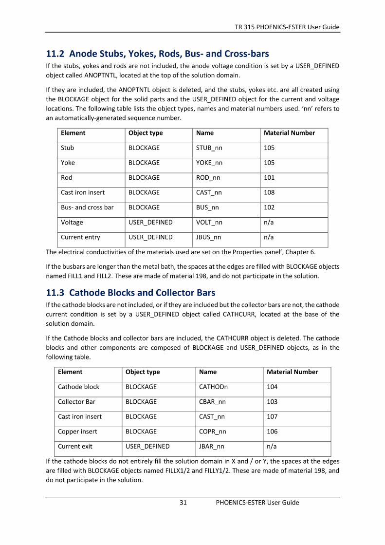
12.1 Displaying the metal - electrolyte interface There are several ways to display the metal – electrolyte interface. One way is to plot a contour map
of the variable HI. Switch the plotting plane to Z and move the probe to the plane immediately below
the interface. Select HI as the plotting variable, and turn on the contour display by clicking the contour
icon . Right-click this icon, and increase the minimum value until the first white space appears in
the blue zone, then decrease a fraction until it disappears. Decrease the maximum value until the first
white space appears in the red zone, then increase a fraction. The contour map should now be scaled
to the minimum and maximum heights of the interface.
Original scale Adjusted scale
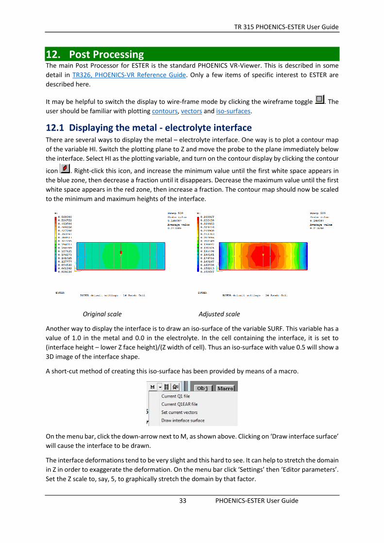
Another way to display the interface is to draw an iso-surface of the variable SURF. This variable has a
value of 1.0 in the metal and 0.0 in the electrolyte. In the cell containing the interface, it is set to
(interface height – lower Z face height)/(Z width of cell). Thus an iso-surface with value 0.5 will show a
3D image of the interface shape.
A short-cut method of creating this iso-surface has been provided by means of a macro.
On the menu bar, click the down-arrow next to M, as shown above. Clicking on ‘Draw interface surface’
will cause the interface to be drawn.
The interface deformations tend to be very slight and this hard to see. It can help to stretch the domain
in Z in order to exaggerate the deformation. On the menu bar click ‘Settings’ then ‘Editor parameters’.
Set the Z scale to, say, 5, to graphically stretch the domain by that factor.
TR 315 PHOENICS-ESTER User Guide
34 PHOENICS-ESTER User Guide
Actual proportions Z scale increased by factor 5
To switch the iso-surface off, click the iso-surface icon .
Yet another way is to plot contours of the additional variable HINT
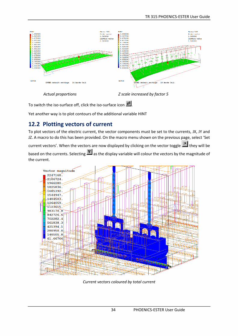
12.2 Plotting vectors of current To plot vectors of the electric current, the vector components must be set to the currents, JX, JY and
JZ. A macro to do this has been provided. On the macro menu shown on the previous page, select ‘Set
current vectors’. When the vectors are now displayed by clicking on the vector toggle they will be
based on the currents. Selecting as the display variable will colour the vectors by the magnitude of
the current.
Current vectors coloured by total current
TR 315 PHOENICS-ESTER User Guide
35 PHOENICS-ESTER User Guide
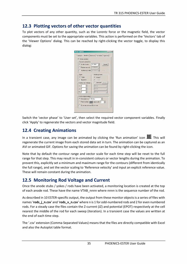
12.3 Plotting vectors of other vector quantities To plot vectors of any other quantity, such as the Lorentz force or the magnetic field, the vector
components must be set to the appropriate variables. This action is performed on the ‘Vectors’ tab of
the ‘Viewer Options’ dialog. This can be reached by right-clicking the vector toggle, to display this
dialog:
Switch the ‘vector phase’ to ‘User set’, then select the required vector component variables. Finally
click ‘Apply’ to regenerate the vectors and vector magnitude field.
12.4 Creating Animations
In a transient case, any image can be animated by clicking the ‘Run animation’ icon . This will
regenerate the current image from each stored data set in turn. The animation can be captured as an
AVI or animated GIF. Options for saving the animation can be found by right-clicking the icon.
Note that by default the contour range and vector scale for each time step will be reset to the full
range for that step. This may result in in-consistent colours or vector lengths during the animation. To
prevent this, explicitly set a minimum and maximum range for the contours (different from identically
the full range), and set the vector scaling to ‘Reference velocity’ and input an explicit reference value.
These will remain constant during the animation.
12.5 Monitoring Rod Voltage and Current Once the anode stubs / yokes / rods have been activated, a monitoring location is created at the top
of each anode rod. These have the name VTAB_nnnn where nnnn is the sequence number of the rod.
As described in 10 ESTER-specific output, the output from these monitor objects is a series of files with
names ‘rods_j_n.csv’ and ‘rods_v_n.csv’ where n is 1 for odd-numbered rods and 2 for even numbered
rods. For a steady case the files contain the Z-current (JZ) and potential (EPOT) respectively at the cell
nearest the middle of the rod for each sweep (iteration). In a transient case the values are written at
the end of each time step.
The ‘.csv’ extension (Comma-Separated Values) means that the files are directly compatible with Excel
and also the Autoplot table format.

TR 315 PHOENICS-ESTER User Guide
36 PHOENICS-ESTER User Guide
12.6 Monitoring Collector-bar currents As described in 10 ESTER-Specific Output, the current drawn from each end of each collector bar can
be monitored in the file ‘cbars_1.csv’ for odd-numbered exit points, and ‘cbars_2.csv’ for even-
numbered exit points.
12.7 Monitoring the Interface Height There are three independent means of monitoring the evolution of the interface height with sweep
for steady cases or with step for transient cases.
As described in 12.1 Displaying the metal-electrolyte interface, create an iso surface of the
interface. Click the Animate’ button to redraw the image from each saved set of
results. As long as the sweep/step frequency of dumping on the ‘Field dumping – settings’
panel of the Main Menu Output panel is set >0, this will produce an animation of the
interface height motion.
As described in 10 ESTER-Specific Output, activate the generation of interface-height files
every n sweeps or steps. Display the interface height maps in 3rd party software.
As described in 10 ESTER-Specific Output, activate up to 5 interface-height monitor points.
Display the change of interface height at these locations in Excel or Autoplot.
As described in 10 ESTER-Specific Output, activate storage of the relative interface height
HINT. Create a contour map at any Z location (they are all the same), then click the
Animate’ button to redraw the image from each saved set of results. As long as the
sweep/step frequency of dumping on the ‘Field dumping – settings’ panel of the Main
Menu Output panel is set >0, this will produce an animation of the interface height motion.

TR 315 PHOENICS-ESTER User Guide
37 PHOENICS-ESTER User Guide
13. Q1 Settings The Q1 settings for a case with anodes, stubs, busbars, cathode blocks, collector bars and cast-iron
inserts is shown here. If an item is set to NO, then the subsequent data settings will be absent.
13.1 Domain Settings The carbon blocks are included: > DOM, CARBON-BLOCKS,YES
The name of the default geometry file > DOM, CATHODE-GEOM, default
The number of cathode blocks > DOM, NUM-BLOCKS, 14
The block size in X, Y and Z > DOM, BLOCK-SIZE, 7.030000E-01, 3.000000E+00, 4.500000E-01
The collector bars are included > DOM, COLLECTOR-BAR,YES
The number of collector bars per cathode block > DOM, NUM-BARS, 1
The size of the collector bars in X, Y and the central gap > DOM, BAR-SIZE, 1.500000E-01, 1.600000E-01, 2.000000E-01
The copper inserts are included > DOM, COPPER-INSERT,YES
The copper insert size in X, Y and Z and the edge offset > DOM, INSERT-SIZE, 5.000000E-02, 1.300000E+00, 6.000000E-02, 1.000000E-01
The cast-iron inserts around the collector bars are included > DOM, CAST-IRON-INS,YES
The thickness of the inserts > DOM, INSERT-THICK, 5.000000E-03
The anodes are included > DOM, ANODES, YES
The number of anodes in X and Y > DOM, NUM-ANODES, 12, 2
The size of the anode, the edge gap and inter-anode gap in X then Y > DOM, SIZE-X, 7.700000E-01, 4.000000E-02, 1.600000E-01
> DOM, SIZE-Y, 1.400000E+00, 1.000000E-01, 1.000000E-01
The depth of metal and anode height > DOM, SIZE-Z-1, 2.000000E-01, 4.000000E-01
The depth of electrolyte and ACD > DOM, SIZE-Z-2, 2.000000E-01, 4.000000E-02
The tapping gaps are included in X, gap size, number of cells in gap, after anode(s) > DOM, TAPPING-GAP, YES, X, 1.000000E-01, 1, 6, 7
The anode yoke configuration > DOM, YOKE-CONFIG, 1*3

TR 315 PHOENICS-ESTER User Guide
38 PHOENICS-ESTER User Guide
The anode stub diameter, depth of insertion into anode and distance from top of carbon to top of
yoke > DOM, ANODE-STUB, 1.300000E-01, 1.000000E-01, 3.500000E-01
Size of yoke in X, Y and Z > DOM, ANODE-YOKE, 1.200000E-01, 8.100000E-01, 1.500000E-01
Size of anode rod in X, Y and Z, and length of steel at end of rod > DOM, ANODE-ROD, 1.200000E-01, 1.200000E-01, 1.500000E+00, 1.000000E-01
The cast-iron inserts around the anode stubs are included > DOM, STUB-LAYER, YES
The layer thickness > DOM, LAYER-SIZE, 5.000000E-03
The busbars are included > DOM, BUSBARS, YES
The number of busbars (in Y), the number of cross bars (in X), the number of side current entry-
points and the number of end current entry-points > DOM, NUM-BUSBARS, 2, 4 , 4, 2
The busbar size in X, Y and Z > DOM, BUS-SIZE, 9.680000E+00, 1.200000E-01, 3.000000E-01
The size of each cross bar in X and the centre location in X relative to the busbar origin, repeated for
each cross bar where n is the sequence number of the cross bar > DOM, BAR-SIZE-0n, 1.200000E-01, 5.999994E-02
The size of each side current entry-point in X and the centre location in X relative to the busbar
origin, repeated for each side entry where n is the sequence number of the entry-point > DOM, SIDE-ENTRY-0n, 1.200000E-01, 5.999994E-02
The size of each end current entry-point in Y and the centre location in Y relative to the busbar origin,
repeated for each end entry where n is the sequence number of the entry-point > DOM, END-ENTRY-0n, 1.200000E-01, 5.999994E-02, 0
The number of cells in the anode, edge gaps and interanode gaps in X then in Y > DOM, NUM-X, 10, 2, 2
> DOM, NUM-Y, 16, 2, 2
The number of Z cells below the copper inserts, in the copper inserts and collector bar above the
copper. > DOM, NUM-Z-1, 2, 2, 5
The number of Z cells in the electrolyte, metal below the anodes, metal at anode immersion, and
anodes above the bath > DOM, NUM-Z-2, 5, 3, 4, 3
The number of Z cells in the yoke, rod and busbars > DOM, NUM-Z-3, 5, 10, 2
The freeze ledge is included > DOM, FREEZE, YES
The freeze-toe to anode edge distance > DOM, FREEZE-TOE, 0.000000E+00

TR 315 PHOENICS-ESTER User Guide
39 PHOENICS-ESTER User Guide
The Lorentz forces are ON > DOM, LORENTZ, ON
ESTER auto-meshing is ON > DOM, AUTOMESH, ON
The interface is initially flat > DOM, INTERFACE, FLAT
The alternative settings are SLOPE_IN_X, SLOPE_IN_Y or READ_FROM_FILE. The initial displacements
at either end are then held in RG(16) and RG(17). The file name is held in
SPDAT(SET,ESTER,HUMP,C,file_name)
The total cell current in Amps > DOM, CELL-CURRENT, 2.000000E+05
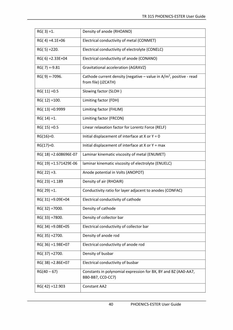
13.2 Variables Passed to ESTRGR In addition, many values are passed to the ESTER Ground station using the LG, IG and RG arrays. The
following table lists the default values of these variables and their meanings. The variable names used
for some variables in earlier versions of ESTER are given in brackets.
Variable Name Function
LG( 1) = T Induced current calculation active
LG( 2) = T Free surface adjustment active
LG( 3) = T Include Loretz force in interface adjustment
LG( 4) = T ACD constant
IG( 1) = 14 Last IZ plane in metal (IZ1)
IG( 2) = 17 IZ plane under anodes (IZ2)
IG( 3) = 1 Interface height adjustment frequency (NIH)
IG( 4) = 1 First sweep for interface adjustment (IHF)
IG( 6) = 21 Last IZ plane in air space above bath (IZ3)
IG(11)=0 If >0, read height of anode undersides from file – see Appendix B
(HANO)
IG(12)=0 If >0, read initial interface height distribution from file – see
Appendix D (HUMP)
IG( 13) = 9 Last IZ plane in cathode block (IZ0)
IG( 14) = 2 Magnetic field units flag (0-Tesla, 1-Gauss, 2-milliTesla) (IMAGU)
IG( 15) = 1 Magnetic field formula switch (0-linear, 1-polynomial) (IMAGF)
RG( 1) =2300. Density of metal (RHOMET)
RG( 2) =2100. Density of electrolyte (RHOELC)
TR 315 PHOENICS-ESTER User Guide
40 PHOENICS-ESTER User Guide
RG( 3) =1. Density of anode (RHOANO)
RG( 4) =4.1E+06 Electrical conductivity of metal (CONMET)
RG( 5) =220. Electrical conductivity of electrolyte (CONELC)
RG( 6) =2.33E+04 Electrical conductivity of anode (CONANO)
RG( 7) =-9.81 Gravitational acceleration (AGRAVZ)
RG( 9) =-7096. Cathode current density (negative – value in A/m2, positive - read
from file) (JZCATH)
RG( 11) =0.5 Slowing factor (SLOH )
RG( 12) =100. Limiting factor (FDH)
RG( 13) =0.9999 Limiting factor (FHLIM)
RG( 14) =1. Limiting factor (FRCON)
RG( 15) =0.5 Linear relaxation factor for Lorentz Force (RELF)
RG(16)=0. Initial displacement of interface at X or Y = 0
RG(17)=0. Initial displacement of interface at X or Y = max
RG( 18) =2.608696E-07 Laminar kinematic viscosity of metal (ENUMET)
RG( 19) =1.571429E-06 laminar kinematic viscosity of electrolyte (ENUELC)
RG( 22) =3. Anode potential in Volts (ANOPOT)
RG( 23) =1.189 Density of air (RHOAIR)
RG( 29) =1. Conductivity ratio for layer adjacent to anodes (CONFAC)
RG( 31) =9.09E+04 Electrical conductivity of cathode
RG( 32) =7000. Density of cathode
RG( 33) =7800. Density of collector bar
RG( 34) =9.08E+05 Electrical conductivity of collector bar
RG( 35) =2700. Density of anode rod
RG( 36) =1.98E+07 Electrical conductivity of anode rod
RG( 37) =2700. Density of busbar
RG( 38) =2.86E+07 Electrical conductivity of busbar
RG(40 – 67) Constants in polynomial expression for BX, BY and BZ (AA0-AA7,
BB0-BB7, CC0-CC7)
RG( 42) =12.903 Constant AA2

TR 315 PHOENICS-ESTER User Guide
41 PHOENICS-ESTER User Guide
RG( 46) =-0.465 Constant AA6
RG( 51) =-4. Constant BB1
RG( 57) =0.832 Constant BB7
RG( 64) =-1.032 Constant CC4
RG( 71) =7800. Density of anode stub
RG( 72) =2.17E+06 Electrical conductivity of anode stub
RG( 73) =8950. Density of copper insert
RG( 74) =1.34E+07 Electrical conductivity of copper insert
RG( 75) =7800. Density of cast iron insert in anode
RG( 76) =6.45E+05 Electrical conductivity of cast iron insert in anode
RG( 77) =7800. Density of cast iron insert in cathode
RG( 78) =8.7E+05 Electrical conductivity of cast iron insert in cathode
13.3 Anode Object The specific settings for an anode object are:
Set object type to ANODE > OBJ, TYPE, ANODE
Anode is not active – (line not written for active anodes) > OBJ, ACTIVE, NO
Anode is raised by n cells – (line not written for un-raised anodes) > OBJ, RAISED, YES, n
The material of an ANODE object is always set to 100.
13.4 Additional Monitoring flags Generate interface height file: SPEDAT(SET,ESTER,HI-FILE,C,YES)
Interface-height file dumping frequency: SPEDAT(SET,ESTER,HI-FREQ,I,ifreq)
Individual height-monitor plots active: SPEDAT(SET,ESTER,HI-MON,C,YES)
Height-monitor locations: SPEDAT(SET,ESTER,HI-MON-X-n,R,Xcoor)
SPEDAT(SET,ESTER,HI-MON-Y-n,R,Ycoor)
Generate collector-bar currents file: SPEDAT(SET,ESTER,CBARJ-FILE,C,YES)

TR 315 PHOENICS-ESTER User Guide
42 PHOENICS-ESTER User Guide
Generate anode-rods currents file: SPEDAT(SET,ESTER,RODSJ-FILE,C,YES)
Generate anode-rods voltage file: SPEDAT(SET,ESTER,RODSV-FILE,C,YES)

TR 315 PHOENICS-ESTER User Guide
43 PHOENICS-ESTER User Guide
Appendix A. Mathematical Background
A.1 Some notes on the solution of the General Conservation
Equation PHOENICS solves a general conservation equation, which for a single phase flow may be written as:
𝜕(𝜌)
𝜕𝑡+ ∇(𝜌𝑢 − ∇) = 𝑆
Where the symbols are as defined below:
- The conserved quantity in question (e.g. momentum, energy, mass etc.)
- Density
u -- Velocity vector
- Diffusive exchange coefficient
S - Source term
The source term and exchange coefficient vary from equation to equation, and also from case to case.
Examples of source term are pressure gradient and gravity force for the momentum equations, or
kinetic heating for the enthalpy equation. The mass continuity equation can also be written in the
above form by setting =1 and =0.
The commonly appearing sources, such as those mentioned above, are pre-programmed into the
PHOENICS solver, EARTH. Provision is then made to enable users to add in any further sources
required.
The partial differential equation above is integrated over 'control volumes' (cells) to form the Finite
Volume Equation that is actually solved. The linkage between velocity, pressure and continuity is
resolved by a variant of the SIMPLE algorithm.
A.2 Momentum Sources In a Hall Cell, the flow is primarily driven by the Lorentz forces. These are added to the standard
momentum equations through the ESTER Ground station. The Lorentz forces are computed from the
cross product of the electric current J and the magnetic field B,
𝐹 = 𝐽 × 𝐵
Or explicitly writing the cross product in terms of x y and z components, this becomes:
𝐹𝑥 = 𝐽𝑦𝐵𝑧 − 𝐽𝑧𝐵𝑦
𝐹𝑦 = 𝐽𝑧𝐵𝑥 − 𝐽𝑥𝐵𝑧
𝐹𝑧 = 𝐽𝑥𝐵𝑦 − 𝐽𝑦𝐵𝑥
These forces are then applied to the momentum equations as source terms. Laminar or turbulent
friction is applied at the cathode, and on the anode undersides.
A.3 The Potential Equation and Current Calculations The potential equation is obtained from the standard conservation equation by removing the built-in
sources, and convective and transient terms. The remaining, diffusive, term then contains the electrical
conductivity.

TR 315 PHOENICS-ESTER User Guide
44 PHOENICS-ESTER User Guide
Finally, the currents are deduced in the ESTER Ground station as the gradients of the electric potential:
𝐽 = −𝜎∇𝐸
In terms of components, this is:
𝐽𝑥 = −𝜎(𝐸𝑒 − 𝐸𝑝)/𝛿𝑋𝑔
𝐽𝑦 = −𝜎(𝐸𝑛 − 𝐸𝑝)/𝛿𝑌𝑔
𝐽𝑧 = −𝜎(𝐸ℎ − 𝐸𝑝)/𝛿𝑍𝑔
Where: Xg, Yg and Zg are the distances between cell centres in the x, y and z directions.
In addition, the induced currents arising from the motion of the liquid through the magnetic field are
calculated from:
𝐽𝑖 = 𝜎(𝑉 × 𝐵)
In terms of x y and z components, this is:
𝐽𝑖𝑥 = 𝜎(𝑉𝐵𝑧 − 𝑊𝐵𝑦)
𝐽𝑖𝑦 = 𝜎(𝑊𝐵𝑥 − 𝑈𝐵𝑧)
𝐽𝑖𝑧 = 𝜎(𝑈𝐵𝑦 − 𝑉𝐵𝑥)
The total current is then J + Ji. (The calculation of Ji is controlled by the variable LG(1). When set to T,
the induced currents are calculated, when left at F, they are not).
The potential, being a scalar, is stored at the cell centres. The currents, being components of a vector,
are stored at the cell faces. This results in complications at the Lorentz force stage, as none of the
currents is stored at a convenient location. Hence in the calculation of the Lorentz force, for each
current component four currents must be averaged to the relevant cell face, taking into account non-
uniformities of the grid.
A.4 Potential Equation Sources The boundary conditions for the potential equation are:
Fixed current at the cathode; and,
Fixed potential at the anode.
This is equivalent to fixed mass flux and fixed pressure respectively.
The cathode current can either be set to a constant value, or a distribution can be read in from a file
containing cell by cell values over the cathode. It is left to the user to specify these values appropriately.
The values should be specified in Amps/m2.
Note that if freeze is present, the cathode currents under the freeze should be set to zero. The freeze
is a very poor conductor, and huge potentials will result. These may lead to numerical overflow.
If the collector bars are not included, the setting of cathode current is controlled by the variable JZCATH
(RG(9)) in Q1. This was always the practice in previous versions of ESTER.
The variable can take the following values:
TR 315 PHOENICS-ESTER User Guide
45 PHOENICS-ESTER User Guide
JZCATH < 0 - cathode current density set to uniform value of JZCATH.
JZCATH > 0 - cathode current densities read in from file CG(2) attached to logical unit JZCATH.
If CG(2) is set to Q1, the data can be included in Q1, starting in column 3 or more. The start of the data
is marked with *JZC in column 3. CG(2) can only be 4 characters long. To use a file name up to 30
characters long, the file name can be set as SPEDAT(SET,ESTER,JZCATH,C,file_name).
A USER_DEFINED object named CATHCURR is created at the base of the domain. The object has a
related PATCH command which sets the current:
This patch is attached to object CATHCURR
PATCH(CATHCURR, LOW, -1, 0, 0, 0, 0, 0, 1, 1)
COVAL(CATHCURR, EPOT, FIXFLU, GRND)
If the collector bars are included, the above settings are not used. In this case, the CATHCURR object
and CATHCUR patch are deleted. A USER_DEFINED object named JBAR_nn is created at each end of
each collector bar. Each such object has an associated PATCH which sets the current density. The
current density at each end of a bar is calculated from the bar current divided by the cross-sectional
area of the collector bar.
If the collector bars are not included, but the busbars are included, the value of JZCATH is deduced
from the total cell current divided by the combined area of the cathode blocks (or the freeze-free plan
area of the domain if the cathode blocks are not included).
If the yokes, stubs, rods and busbars are not included, the anode potential is set to a single constant
value in all anodes. This is done in the subroutine POTENT, which is supplied as a model. If the user
wishes to update anode potentials, then POTENT can be used as a 'junction box', to interface to some
other software suite which would supply the potentials.
A USER_DEFINED object called ANOPTNTL is created at the top of the domain. A related patch
ANOPTNT then sets the potential:
This patch is attached to object ANOPTNTL
PATCH(ANOPTNT, HIGH, -1, 0, 0, 0, 0, 0, 1, 1)
COVAL(ANOPTNT, EPOT, GRND, GRND)
The potential is set at the centre of the high face of the top slab of the domain for those cells containing
anode material. The anode potential is held in RG(22) in Q1.
If the anode yokes, stubs and rods are included, the ANOPTNTL object and associated ANOPTNT patch
are deleted. A USER_DEFINED object named VOLT_nn is created at the top of each anode rod, and an
associated patch fixes the potential to the rod potential.
Further, if the busbars are also included, then a USER_DEFINED object called JBUS_nn is created at
each current-entry location, and a fixed-current condition is set by an associated patch. The current is
deduced from the entry-point current divided by the cross-sectional area of the entry-point. In
addition, a single fixed-potential condition is applied at the midpoint of the left-most (in X) cross bar.
This is done by a USER_DEFINED object called VOLT_nn and associated patch.
A further source for the potential equation arises from the induced currents. This source takes the
form:
𝑆 = ∇𝐽𝑖

TR 315 PHOENICS-ESTER User Guide
46 PHOENICS-ESTER User Guide
This is written in finite-difference form as:
𝑆 = (𝐴𝑛𝐽𝑖𝑦)𝑝 − (𝐴𝑛𝐽𝑖𝑦)𝑠 + (𝐴𝑒𝐽𝑖𝑥)𝑝 − (𝐴𝑒𝐽𝑖𝑥)𝑤 + (𝐴ℎ𝐽𝑖𝑧)𝑝 − (𝐴ℎ𝐽𝑖𝑧)𝑙
where the subscript 'p' denotes the current cell, and 'w','s','l' denote the neighbours in the low x, low
y and low z directions. Ae, An and Ah are the cell face areas.
If the induced currents are not calculated, i.e. LG(1)=F, the source is set to zero.
A.5 Magnetic Fields To avoid the interpolation complications associated with the current components, the B field
components are deemed to be stored at the cell centres, even though they too are strictly vectors.
The values of Bx, By and Bz can either be calculated from simple algebraic expressions, or individual cell
values can be read in from a data file. The fields can be specified in Gauss, Tesla or milliTesla. Internally,
the values are always converted to Tesla.
The expressions used are a linear formula:
Bx = A0 (1 – 2Y/Ymax)
By = B0 (1 – 2X/Xmax)
Bz = C0 (1 – 2X/Xmax) (1 – 2Y/Ymax)
or a polynomial formula:
Bx = A0 + A1 X + A2 Y + A3 X2 + A4 XY + A5 Y2 + A6 X2Y + A7 XY2
By = B0 + B1 X + B2 Y + B3 X2 + B4 XY + B5 Y2 + B6 X2Y + B7 XY2
Bz = C0 + C1 X + C2 Y + C3 X2 + C4 XY + C5 Y2 + C6 X2Y + C7 XY2
The coefficients A0 – A7 are held as RG(40) – RG(47) in Q1.
The coefficients B0 – B7 are held as RG(50) – RG(57) in Q1.
The coefficients C0 – C7 are held as RG(60) – RG(67) in Q1.
There is at present no provision for updating the B field, but this can easily be done from Group 19 of
the Ground station, if a suitable physical mechanism is known.
The setting of the B field is controlled by the variable MAGF (IG(5) in Q1). This can take the following
values:
MAGF = 0 - B fields calculated from algebraic expressions in Group 11 of the ESTER Ground station.
MAGF > 0 - B fields read in from file CG(1) attached to logical unit MAGF.
If CG(1) is set to Q1, the data can be included in Q1, starting in column 3 or more. The start of the data
is marked with *MAGF in column 3.
CG(1) can only be 4 characters long. To use a file name up to 30 characters long, the file name can be
set as SPEDAT(SET,ESTER,MAGF,C,file_name).
TR 315 PHOENICS-ESTER User Guide
47 PHOENICS-ESTER User Guide
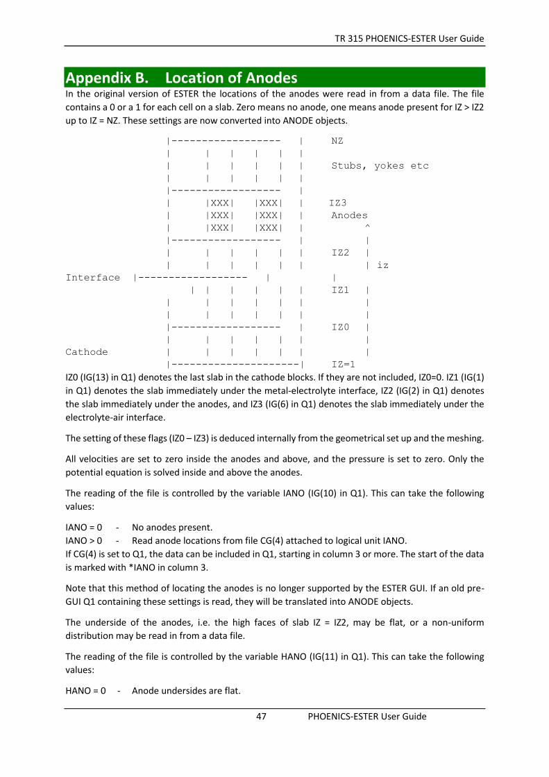
Appendix B. Location of Anodes In the original version of ESTER the locations of the anodes were read in from a data file. The file
contains a 0 or a 1 for each cell on a slab. Zero means no anode, one means anode present for IZ > IZ2
up to IZ = NZ. These settings are now converted into ANODE objects.
|------------------ | NZ
| | | | | |
| | | | | | Stubs, yokes etc
| | | | | |
|------------------ |
| |XXX| |XXX| | IZ3
| |XXX| |XXX| | Anodes
| |XXX| |XXX| | ^
|------------------ | |
| | | | | | IZ2 |
| | | | | | | iz
Interface |------------------ | |
| | | | | | IZ1 |
| | | | | | |
| | | | | | |
|------------------ | IZ0 |
| | | | | | |
Cathode | | | | | | |
|---------------------| IZ=1
IZ0 (IG(13) in Q1) denotes the last slab in the cathode blocks. If they are not included, IZ0=0. IZ1 (IG(1)
in Q1) denotes the slab immediately under the metal-electrolyte interface, IZ2 (IG(2) in Q1) denotes
the slab immediately under the anodes, and IZ3 (IG(6) in Q1) denotes the slab immediately under the
electrolyte-air interface.
The setting of these flags (IZ0 – IZ3) is deduced internally from the geometrical set up and the meshing.
All velocities are set to zero inside the anodes and above, and the pressure is set to zero. Only the
potential equation is solved inside and above the anodes.
The reading of the file is controlled by the variable IANO (IG(10) in Q1). This can take the following
values:
IANO = 0 - No anodes present.
IANO > 0 - Read anode locations from file CG(4) attached to logical unit IANO.
If CG(4) is set to Q1, the data can be included in Q1, starting in column 3 or more. The start of the data
is marked with *IANO in column 3.
Note that this method of locating the anodes is no longer supported by the ESTER GUI. If an old pre-
GUI Q1 containing these settings is read, they will be translated into ANODE objects.
The underside of the anodes, i.e. the high faces of slab IZ = IZ2, may be flat, or a non-uniform
distribution may be read in from a data file.
The reading of the file is controlled by the variable HANO (IG(11) in Q1). This can take the following
values:
HANO = 0 - Anode undersides are flat.

TR 315 PHOENICS-ESTER User Guide
48 PHOENICS-ESTER User Guide
HANO > 0 - Read anode underside heights from file CG(5) attached to logical unit HANO.
If CG(5) is set to Q1, the data can be included in Q1, starting in column 3 or more. The start of the data
is marked with *HANO in column 3.
CG(5) can only be 4 characters long. To use a file name up to 30 characters long, the file name can be
set as SPEDAT(SET,ESTER,HANO,C,file_name).
Under some circumstances, the anode undersides may take on the shape of the metal-electrolyte
interface. This situation, known as 'burn-off', may be modelled by setting LG(4) = T. The distance
between the anodes and the interface will now be kept constant at the initial value irrespective of the
motion of the interface.

TR 315 PHOENICS-ESTER User Guide
49 PHOENICS-ESTER User Guide
Appendix C. Freeze The freeze is the solid accretion around the edges of the cell, which reduces the volume and the
available cathode area. The presence of freeze is accounted for by fixing the velocities and pressure to
zero in selected cells. The potential is also fixed to zero within the freeze, as it is such a poor conductor.
The location and height of the freeze was read in from a data file. The file contained the height, in full
Z slabs, of freeze in each column of cells. The freeze may extend up into the electrolyte layer.
The reading of the file was controlled by the variable IFRZ. This can take the following values:
IFRZ = 0 - No freeze present.
IFRZ > 0 - Read freeze heights from file CG(3) attached to logical unit IFRZ.
If CG(3) is set to Q1, the data can be included in Q1, starting in column 3 or more. The start of the data
is marked with *IFRZ in column 3.
Note that this method of locating the freeze is no longer supported by the ESTER GUI. If an old pre-GUI
Q1 containing these settings is read, they will be translated into blockage objects.
The modelling of the freeze was very simple - no partial cell occupation is allowed, and freeze will rise
and fall with the interface, as the height is specified in terms of slabs, not actual height.
In the current ESTER, the freeze ledges are modelled as sloped non-conductive blockages at the
domain edges.

TR 315 PHOENICS-ESTER User Guide
50 PHOENICS-ESTER User Guide
Appendix D. The Moving Grid and the Metal-Electrolyte Interface
As discussed in the introduction, the primary feature of the Hall Cell is the presence of two distinct
layers of fluid, which never mix. Lorentz forces deform the interface between these two layers of fluid
and the enormous difference in conductivity across them means that even small height fluctuations
can significantly alter the resistance paths, and hence current distributions. This then feeds back to the
Lorentz forces and the height distribution.
In ESTER, the interface is always maintained at the high faces of the slab IZ = IZ1. The grid is then
stretched to follow the motion of the interface. The grid itself does not actually change, but the North
and East porosities, and the z direction inter-nodal distances, are adjusted to give the same effect. This
is considerably cheaper computationally than using a distorting BFC grid. The adjustment takes place
in the slabs between IZ0 and IZ3. Slabs in the cathode blocks and above the bottom face of the anodes
are not adjusted.
The interface adjustment is based on the principle of maintaining hydrostatic equilibrium across the
interface. A reference cell is chosen (the first unblocked cell), and height adjustments are calculated
for all other cells based on the pressure difference between the reference cells above and below the
interface. Once the adjustments have been applied, the whole interface is moved up or down by a
uniform amount in order to preserve the open volume under it. The adjustment sequence is entered
every NIH sweeps, once ISWEEP > IHF.
A similar adjustment can be performed at the electrolyte free surface, where the inter-anode gaps are
open to the atmosphere. This can be switched on by setting LG(2) = T.
The vertically directed components of the Lorentz force can be included in the balance equation across
the interface by setting LG(3) = T.
The initial distribution of the interface height may be read from a file. This is signalled by setting IG(12)
> 0 - Read anode underside heights from file CG(6) attached to logical unit IG(12).
If CG(6) is set to Q1, the data can be included in Q1, starting in column 3 or more. The start of the data
is marked with *HUMP in column 3.
CG(6) can only be 4 characters long. To use a file name up to 30 characters long, the file name can be
set as SPEDAT(SET,ESTER,HUMP,C,file_name).
The true (i.e. distorted) heights of the cell faces are stored in the variable HI. A PHOTON contour map
of the interface can thus be obtained by plotting contours of HI at IZ = IZ1. It is best to SET CON SCALE
PLANE prior to this, as the changes in height on a plane are usually very small.
The variable SURF contains a relief map of the interface – an iso-surface of SURF with the value 0.5 will
show a 3D surface of the interface.

TR 315 PHOENICS-ESTER User Guide
51 PHOENICS-ESTER User Guide
Appendix E. ESTER File Formats The files making up ESTER have the following significances:
ESTRGR.FOR - The ESTER Ground Station. This should be studied together with the Q1 file. It can be
found in phoenics/d_earth/d_spe/d_ester.
Several example Q1 files are supplied as library cases Y400 – Y412, and Y497. , setting up a twenty-four
anode case. These can be found at /phoenics/d_earth/d_spe/d_mscspp/inplib.
The input files described below primarily refer to previous versions of ESTER. The descriptions are left
for completeness. Only the magnetic field, cathode-current and anode-underside-height files may be
used by the current ESTER.
As noted above, the files referred to below may be physically appended to the Q1 file after the STOP
line, and not exist as separate files. If they are embedded in Q1 before STOP, then the lines containing
the data must be after a PIL comment line (staring column 3) SAVE11BEGIN, and before a PIL comment
line SAVE11END.
The Freeze - FRZ (deprecated)
A data file defining the locations and height in IZ slabs of the freeze. The file is appended to the end of
the library Q1. The freeze may extend above the interface at IZ1. The numbers indicate the height (in
Z slabs) of the freeze in each IX,IY column.
1 1 1 1 1 1 1 1 1 1
1 0 0 0 0 0 0 0 0 1
1 0 0 0 0 0 0 0 0 1
1 0 0 0 0 0 0 0 0 1
1 0 0 0 0 0 0 0 0 1
1 0 0 0 0 0 0 0 0 1
1 0 0 0 0 0 0 0 0 1
^ 1 0 0 0 0 0 0 0 0 1
IY | 1 0 0 1 1 0 0 0 0 1
| 2 1 1 1 1 1 1 1 1 1
|____>
IX
(IX is along this direction >>>> and IY vertically).
The Cathode Currents - JZC
A data file defining the cathode current distribution. It is important to specify zero cathode current
within the freeze, otherwise overflow may result.
Data Format 1 (Deprecated)
The library example is shown below. The numbers specify the current in Amps/m2 passing through the
centre of each cell face adjacent to the cathode. This is always located at z=0, i.e. low of IZ=1.
0. 0. 0. 0. 0. 0. 0. 0. 0. 0.
0. -5000. -5000. -5000. -5000. -5000. -5000. -5000. -5000. 0.
0. -5000. -5000. -5000. -5000. -5000. -5000. -5000. -5000. 0.
0. -5000. -5000. -5000. -5000. -5000. -5000. -5000. -5000. 0.
0. -5000. -5000. -5000. -5000. -5000. -5000. -5000. -5000. 0.
0. -5000. -5000. -5000. -5000. -5000. -5000. -5000. -5000. 0.
0. -5000. -5000. -5000. -5000. -5000. -5000. -5000. -5000. 0.
^ 0. -5000. -5000. -5000. -5000. -5000. -5000. -5000. -5000. 0.
IY | 0. -5000. -5000 0. 0. -5000. -5000. -5000. -5000. 0.
| 0. 0. 0. 0. 0. 0. 0. 0. 0. 0.
|---> IX

TR 315 PHOENICS-ESTER User Guide
52 PHOENICS-ESTER User Guide
This format is very inflexible, as it relies on the file containing exactly the correct number of data values.
If the computational grid is changed, the file will not be valid.
Data Format 2 (Recommended)
For this reason, an alternative format is available, in which the X and Y coordinates of each data point
are specified. Once read in, the currents are interpolated onto the grid in use. As a final adjustment,
the interpolated currents are normalised so that the total current is preserved.
The first few lines of such a file are given here as an example:
88 32 4.55E5
-0.70000E+01 -0.20250E+01 0.00000E+00
-0.68391E+01 -0.20250E+01 0.00000E+00
-0.66782E+01 -0.20250E+01 0.00000E+00
-0.65172E+01 -0.20250E+01 0.00000E+00
-0.63563E+01 -0.20250E+01 0.00000E+00
-0.61954E+01 -0.20250E+01 0.00000E+00
The first line contains the number of data points in X (NI), the number of data points in Y (NJ) and the
total current in Amps. The total current can also be specified as the single item on the second line. The
following lines contain the X coordinate, Y coordinate and current density in A/m2 at that point. The
coordinates are in metres, relative to the centre-point of the cathode.
The coordinate and current data is read by loops similar to:
DO J=1,NJ
DO I=1,NI
READ() X(I), Y(J), Jz(I,J)
ENDDO
ENDDO
NI and NJ are the values read from the first line of the data file. Blank lines, lines starting with # and
any characters after ! are ignored, allowing the file to be commented. A two-stage linear interpolation
is performed to get the current at the grid cell centres.
The Anode Locations - ANO (deprecated)
A data file defining the locations of the anodes. The anode locations are actually specified by the
ANODE objects and the anode configuration. The data-file method is retained for downward
compatibility, but anodes defined this way will be converted to ANODE objects at startup. In the file, a
0 means free volume, a 1 means an anode occupies the cell. The active library example for a 4 anode
cell is shown below. The anodes only exist at z locations above IZ = IZ2.
0 0 0 0 0 0 0 0 0 0
0 1 1 1 0 0 1 1 1 0
0 1 1 1 0 0 1 1 1 0
0 1 1 1 0 0 1 1 1 0
0 0 0 0 0 0 0 0 0 0
0 0 0 0 0 0 0 0 0 0
0 1 1 1 0 0 1 1 1 0
^ 0 1 1 1 0 0 1 1 1 0
| 0 1 1 1 0 0 1 1 1 0
| 0 0 0 0 0 0 0 0 0 0
|____> IX
The Anode Underside Heights - HAN
A data file defining the height in metres of the anode undersides above the cathode. The anode
undersides may be flat, sloped or contoured.

TR 315 PHOENICS-ESTER User Guide
53 PHOENICS-ESTER User Guide
Data Format 1 (Deprecated)
The library example for flat anodes is shown below.
0.260 0.260 0.260 0.260 0.260 0.260 0.260 0.260 0.260 0.260
0.260 0.260 0.260 0.260 0.260 0.260 0.260 0.260 0.260 0.260
0.260 0.260 0.260 0.260 0.260 0.260 0.260 0.260 0.260 0.260
0.260 0.260 0.260 0.260 0.260 0.260 0.260 0.260 0.260 0.260
0.260 0.260 0.260 0.260 0.260 0.260 0.260 0.260 0.260 0.260
0.260 0.260 0.260 0.260 0.260 0.260 0.260 0.260 0.260 0.260
0.260 0.260 0.260 0.260 0.260 0.260 0.260 0.260 0.260 0.260
^ 0.260 0.260 0.260 0.260 0.260 0.260 0.260 0.260 0.260 0.260
IY | 0.260 0.260 0.260 0.260 0.260 0.260 0.260 0.260 0.260 0.260
| 0.260 0.260 0.260 0.260 0.260 0.260 0.260 0.260 0.260 0.260
|____>
IX
An alternative set of data shown below, indicates how sloped anodes may be introduced. This data
should be used for 2-phase calculations, as the gas will tend to move up the slopes towards the central
inter-anode gap and then escape.
0.260 0.260 0.260 0.260 0.260 0.260 0.260 0.260 0.260 0.260
0.260 0.260 0.260 0.260 0.260 0.260 0.260 0.260 0.260 0.260
0.267 0.267 0.267 0.267 0.267 0.267 0.267 0.267 0.267 0.267
0.274 0.274 0.274 0.274 0.274 0.274 0.274 0.274 0.274 0.274
0.274 0.274 0.274 0.274 0.274 0.274 0.274 0.274 0.274 0.274
0.274 0.274 0.274 0.274 0.274 0.274 0.274 0.274 0.274 0.274
0.274 0.274 0.274 0.274 0.274 0.274 0.274 0.274 0.274 0.274
^ 0.267 0.267 0.267 0.267 0.267 0.267 0.267 0.267 0.267 0.267
IY | 0.260 0.260 0.260 0.260 0.260 0.260 0.260 0.260 0.260 0.260
| 0.260 0.260 0.260 0.260 0.260 0.260 0.260 0.260 0.260 0.260
|____>
IX
This format is very inflexible, as it relies on the file containing exactly the correct number of data values.
If the computational grid is changed, the file will not be valid.
Data Format 2 (Recommended)
For this reason, an alternative format is available, in which the X and Y coordinates of each data point
are specified. Once read in, the anode-underside heights are interpolated onto the grid in use. The first
few lines of such a file are given here as an example:
56 26
-2.575 -1.285 0.230
-2.475 -1.285 0.230
-2.364 -1.285 0.230
-2.254 -1.285 0.230
-2.143 -1.285 0.230
-2.032 -1.285 0.230
The first line contains the number of data points in X (NI) and the number of data points in Y (NJ) The
following lines contain the X coordinate, Y coordinate and anode-underside height in m at that point.
The coordinates are in metres, relative to the centre-point of the cathode.
The coordinate and height data is read by loops similar to:
DO J=1,NJ
DO I=1,NI
READ() X(I), Y(J), H(I,J)
ENDDO
ENDDO

TR 315 PHOENICS-ESTER User Guide
54 PHOENICS-ESTER User Guide
NI and NJ are the values read from the first line of the data file. Blank lines, lines starting with # and
any characters after ! are ignored, allowing the file to be commented. A two-stage linear interpolation
is performed to get the height at the grid cell centres.
The Magnetic Fields – MAGF
A data file specifying the magnetic field components at the cell faces. This file is not used in the active
demo, as the magnetic fields are computed from algebraic expressions. No example data is provided.
The field components should be defined in Gauss. The field components are deemed to be stored at
the cell centres.
Data Format 1 (Deprecated)
The data is read in the order shown below in the sample code. If the file does not contain data for all
Z planes, the fields are assumed to remain the same at all Z locations above the last plane read. The
following code snippet shows how the values should be ordered.
DO IX=1,NX
DO IY=1,NY
READ() (Bx(IY,IX),By(IY,IX),Bz(IY,IX),IY=1,NY)
ENDDO ENDDO NX, NY are the actual number of cells in X and Y. As with the cathode current file, JZC, this format is
inflexible, as each file describes a particular grid distribution.
Data Format 2 (Recommended)
The recommended format of the magnetic field file is the Tecplot ‘PLT’ format, as shown in the partial
example below:
TITLE=B on_demand
VARIABLES="X","Y","Z","Bx","By","Bz","Bm"
ZONE T="B1", I= 88, J= 32, K= 10,F=POINT
-0.70000E+01 -0.20250E+01 0.00000E+00 -0.13145E-01 0.84991E-02 -0.59068E-02 0.16731E-01
-0.68391E+01 -0.20250E+01 0.00000E+00 -0.14118E-01 0.75620E-02 -0.68962E-02 0.17437E-01
-0.66782E+01 -0.20250E+01 0.00000E+00 -0.16239E-01 0.72623E-02 -0.69125E-02 0.19085E-01
-0.65172E+01 -0.20250E+01 0.00000E+00 -0.17954E-01 0.77459E-02 -0.58176E-02 0.20401E-01
-0.63563E+01 -0.20250E+01 0.00000E+00 -0.16959E-01 0.74316E-02 -0.53471E-02 0.19272E-01
-0.61954E+01 -0.20250E+01 0.00000E+00 -0.18229E-01 0.63882E-02 -0.51384E-02 0.19988E-01
-0.60345E+01 -0.20250E+01 0.00000E+00 -0.18127E-01 0.76131E-02 -0.44052E-02 0.20148E-01
.....
The ‘TITLE’ line is used to identify the file format. The content of TITLE is not used.
The ‘VARIABLES’ line is ignored, and could be absent. It is assumed that the data will be in the order
stated above, i.e. X co-ordinate, Y co-ordinate, Z co-ordinate, X component, Y component, Z
component, magnitude. The coordinates are in metres, relative to the centre-point of the cathode.
The ‘ZONE’ line is used to find the number of data points in X (I= NI), Y (J= NJ) and Z (K= NK). The ‘T=’
and ‘F=’ flags are not used. The remainer of the file is read using loops like:
DO K=1,NK
DO J=1,NJ
DO I=1,NI
READ() XC(I),YC(J),ZC(K), BX(I,J,K),BY(I,J,K),BZ(I,J,K),BM
ENDDO
ENDDO
ENDDO

TR 315 PHOENICS-ESTER User Guide
55 PHOENICS-ESTER User Guide
The Cell Face Locations - GRID.TXT
This is an output file containing the numbers of cells and cell face locations in each coordinate
direction. A very simple example file is shown here:
5 = nx
0.1500 1.8750 2.1250 3.8500 4.0000
9 = ny
0.1500 1.9643 3.7786 5.5929 7.4071 9.2214 11.0357 12.8500 13.0000
5 = nz
0.1000 0.2000 0.2200 0.2400 0.4000
Additional Monitoring
Interface Height: hintn.txt
A sequence of files containing the interface height distribution at sweep or step n. An extract from a
typical file is shown here:
0.0395 0.0992 0.1397 0.1905 0.2577 0.3250 0.3879 0.4526 0.5150
3.1675 0.5963 0.5967 0.5971 0.5976 0.5989 0.6008 0.6027 0.6050 0.6075
3.1445 0.5957 0.5958 0.5962 0.5967 0.5981 0.5998 0.6017 0.6039 0.6064
3.1253 0.5954 0.5953 0.5957 0.5965 0.5981 0.6001 0.6020 0.6041 0.6065
3.1094 0.5951 0.5949 0.5955 0.5966 0.5985 0.6005 0.6024 0.6045 0.6068
3.0960 0.5949 0.5947 0.5954 0.5968 0.5989 0.6011 0.6030 0.6050 0.6073
3.0850 0.5948 0.5946 0.5954 0.5972 0.5995 0.6016 0.6035 0.6055 0.6077
3.0726 0.5947 0.5946 0.5955 0.5977 0.6001 0.6023 0.6041 0.6060 0.6081
3.0562 0.5946 0.5946 0.5957 0.5981 0.6007 0.6029 0.6047 0.6065 0.6085
3.0366 0.5947 0.5948 0.5960 0.5987 0.6013 0.6035 0.6053 0.6070 0.6090
3.0131 0.5949 0.5952 0.5964 0.5993 0.6019 0.6041 0.6058 0.6075 0.6093
2.9849 0.5952 0.5959 0.5970 0.6000 0.6025 0.6045 0.6061 0.6078 0.6095
The first line contains the X co-ordinate for each X location. The subsequent lines contain the Y co-
ordinate as the first entry followed by the interface height at each X location. In the above extract the
red values are X co-ordinates and the green Y co-ordinates.
Individual Height monitor: hi-mon-n.csv
Up to 5 files containing the interface height at a position as a function of sweep or time for transient
cases. An extract from a typical transient file is shown here:
TIME, HI_1
4.000000E+00, 1.727117E-01
8.000000E+00, 1.757539E-01
1.200000E+01, 1.795289E-01
1.600000E+01, 1.836075E-01
2.000000E+01, 1.876970E-01
2.400000E+01, 1.916234E-01
2.800000E+01, 1.953025E-01
3.200000E+01, 1.987072E-01
3.600000E+01, 2.018405E-01
Collector-bar Currents file: cbars_1.csv and cbars_2.csv
Two files containing the odd- and even-numbered collector-bar currents in Amps as a function of
sweep or time. An extract from a typical file is shown here:
ISWEEP, J_01, J_03, J_05, J_07, J_09, J_11, J_13, J_15, J_17, J_19, J_21, J_23, J_25, J_27
1, -7.142855E+03, -7.142853E+03, -7.142855E+03, -7.142849E+03, -7.142861E+03, …
2, -7.142855E+03, -7.142853E+03, -7.142855E+03, -7.142849E+03, -7.142861E+03, …

TR 315 PHOENICS-ESTER User Guide
56 PHOENICS-ESTER User Guide
3, -7.142855E+03, -7.142853E+03, -7.142855E+03, -7.142849E+03, -7.142861E+03, …
4, -7.142855E+03, -7.142853E+03, -7.142855E+03, -7.142849E+03, -7.142861E+03, …
5, -7.142855E+03, -7.142853E+03, -7.142855E+03, -7.142849E+03, -7.142861E+03, …
6, -7.142855E+03, -7.142853E+03, -7.142855E+03, -7.142849E+03, -7.142861E+03, …
7, -7.142855E+03, -7.142853E+03, -7.142855E+03, -7.142849E+03, -7.142861E+03, …
8, -7.142855E+03, -7.142853E+03, -7.142855E+03, -7.142849E+03, -7.142861E+03, …
Anode-rod Currents files: rods_j_1.csv and rods_j_2.csv
Two files containing the currents in the odd- and even-numbered anode rods in Amps/m2 as a function
of sweep or time. An extract from a typical _1 file is shown here:
ISWEEP, J_01, J_03, J_05, J_07, J_09, J_11, J_13, J_15, J_17, J_19, J_21, J_23
1, 0.000000E+00, 0.000000E+00, 0.000000E+00, 0.000000E+00, 0.000000E+00, …
2, -3.831848E+05, -3.812878E+05, -4.118300E+05, -3.942508E+05, -3.805764E+05, …
3, -5.162616E+05, -5.096694E+05, -5.048004E+05, -5.467090E+05, -5.087051E+05, …
4, -3.394898E+05, -3.317594E+05, -2.820572E+05, -3.813668E+05, -3.364071E+05, …
5, -3.064972E+05, -3.004268E+05, -2.610633E+05, -3.474573E+05, -3.081413E+05, …
6, -3.448173E+05, -3.391578E+05, -3.067186E+05, -3.863781E+05, -3.478842E+05, …
7, -4.104862E+05, -4.041154E+05, -3.736206E+05, -4.548452E+05, -4.123042E+05, …
8, -4.754754E+05, -4.677767E+05, -4.330293E+05, -5.233913E+05, -4.747957E+05, …
Anode-rod Voltage files: rods_v_1.csv and rods_v_2.csv
Two files containing the voltages in the odd- and even-numbered anode rods in Volts as a function of
sweep or time. An extract from a typical _1 file is shown here:
ISWEEP, V_01, V_03, V_05, V_07, V_09, V_11, V_13, V_15, V_17, V_19, V_21, V_23
1, 2.992688E+00, 2.992724E+00, 2.991781E+00, 2.992755E+00, 2.992738E+00, …
2, 2.990149E+00, 2.990275E+00, 2.989929E+00, 2.989952E+00, 2.990293E+00, …
3, 2.993522E+00, 2.993669E+00, 2.994379E+00, 2.992990E+00, 2.993581E+00, …
4, 2.994152E+00, 2.994267E+00, 2.994794E+00, 2.993613E+00, 2.994120E+00, …
5, 2.993421E+00, 2.993529E+00, 2.993882E+00, 2.992898E+00, 2.993362E+00, …
6, 2.992168E+00, 2.992289E+00, 2.992547E+00, 2.991640E+00, 2.992133E+00, …
7, 2.990928E+00, 2.991074E+00, 2.991362E+00, 2.990380E+00, 2.990941E+00, …
8, 2.989577E+00, 2.989769E+00, 2.990113E+00, 2.989021E+00, 2.989674E+00, …