Kai XuEpstein Department of Industrial and

Systems Engineering,

University of Southern California,

Los Angeles, CA 90089

Yong Chen1

Epstein Department of Industrial and

Systems Engineering,

University of Southern California,

Los Angeles, CA 90089

e-mail: yongchen@usc.edu

Photocuring Temperature Studyfor Curl Distortion Control inProjection-BasedStereolithographyPolymerization shrinkage and thermal cooling effect have been identified as two majorfactors that lead to the curl distortion in the stereolithography apparatus (SLA) process.In this paper, the photocuring temperature during the building process of mask imageprojection-based stereolithography (MIP-SL) and how it affects parts’ curl distortion areinvestigated using a high-resolution infrared (IR) camera. Test cases of photocuringlayers with different shapes, sizes, and layer thicknesses have been designed and tested.The experimental results reveal that the temperature increase of a cured layer is mainlyrelated to the layer thickness, while the layer shapes and sizes have little effect. The pho-tocuring temperatures of built layers using different exposure strategies including vary-ing exposure time, grayscale levels, and mask image patterns have been studied. The curldistortions of a test case based on various exposure strategies have been measured andanalyzed. It is shown that, by decreasing the photocuring temperature of built layers, theexposure strategies using grayscale levels and mask image patterns can effectivelyreduce the curl distortion with the expense of increased building time. In addition to curldistortion control, the photocuring temperature study also provides a basis for the curldistortion simulation in the MIP-SL process. [DOI: 10.1115/1.4034305]

Keywords: stereolithography, curl distortion, photocuring temperature, processplanning, simulation

1 Introduction

Stereolithography apparatus (SLA) is one of the additive manu-facturing (AM) processes, which has been widely used in variousapplications. In the SLA process, three-dimensional (3D) objectsare built by photocuring liquid resin using controlled light expo-sure. Unlike the laser-based SLA process, the mask imageprojection-based stereolithography (MIP-SL) uses digital micro-mirror device (DMD) to dynamically project mask images ontoliquid resin surface. Since the shape of a whole layer can be curedsimultaneously, the MIP-SL process is much faster than the laser-based SLA process [1]. Compared to other AM processes, MIP-SL has good feature resolution and surface finishes as well [2].Recent breakthrough based on the MIP-SL process has been madeto dramatically increase its building speed up to 100 times [3].However, the MIP-SL process also has some critical challenges.One of such challenges is the curl deformation of the built partsafter removing supported structures. This deformation will lead totolerance loss, making it unacceptable to applications such as withassembly features. Figure 1 shows a rectangular bar built by MIP-SL; in comparison, the nominal shape is shown in dashed lines.From the side view of the built object, such curl deformation isobvious with two tips curl up.

To understand how such curl deformation is formed, someresearchers tried to use finite-element analysis (FEA) and othermodeling methods to simulate the SLA process. Bugeda et al. [4]and Chambers et al. [5] developed an FEA program to simulateSLA deformation. The volumetric shrinkage was incorporatedinto the model. Huang and Jiang [6] and Vatani et al. [7] consid-ered heterogeneous material properties in their simulation models.Some researchers considered the thermal effects during the

building process. Narahara et al. [8] designed an experiment tostudy the relation between linear shrinkage and temperature. Hurand Youn [9] incorporated the thermal cooling effects in the FEAmodel to predict the related deformation in SLA. Tanaka et al.[10] simulated the distortion in SLA by incorporating both ther-mal effect and polymerization shrinkage into the FEA model. Inaddition to the modeling work, some researchers studied thedeformation control in SLA. Huang et al. [11] developed a scan-ning path planning method to increase the accuracy of some diag-nostic parts. Xu and Chen [12] used the mask pattern exposurestrategies to reduce the deformation in built parts. Huang et al.[13–15] increased the accuracy of parts using the reverse compen-sation based on the statistical modeling of measured deformationafter a test part is built.

Although the thermal effect has been identified as one of themajor contributing factors to the deformation of built parts, littleresearch has been reported on the understanding of the curingtemperature during the building process. Previous simulationresearch (e.g., Refs. [8,9]) assumes a constant temperature drop ora certain amount of heat is released when a layer is solidified.

Fig. 1 A physical object built by the MIP-SL process with curldistortion

1Corresponding author.Manuscript received February 23, 2016; final manuscript received July 18, 2016;

published online August 24, 2016. Assoc. Editor: Donggang Yao.

Journal of Manufacturing Science and Engineering FEBRUARY 2017, Vol. 139 / 021002-1Copyright VC 2017 by ASME

Downloaded From: http://manufacturingscience.asmedigitalcollection.asme.org/ on 09/15/2016 Terms of Use: http://www.asme.org/about-asme/terms-of-use

Such an assumption may not be accurate for the projection-basedphotocuring process. In order to better simulate the deformation inthe MIP-SL process, the curing temperature of built layers needsto be measured and studied. Some research reported using embed-ding thermocouples under resin to measure the curing temperatureat discrete points [5,7]. In this paper, a high-precision infrared(IR) camera is adopted to systematically study curing temperatureof the MIP-SL process. We first investigated the curing tempera-ture distribution within a single layer and temperature evolution inmultiple consecutive layers by using IR camera. Then, we furtherstudied the curing temperature related to common MIP-SL pro-cess parameters including exposure time, gray scale values, andmask patterns. Effective exposure strategies based on such curingtemperature study have been designed to reduce the deformationof built parts by reducing the curing temperature of buildinglayers. Similar studies of using IR camera in measuring build sur-face temperature in electronic beam additive manufacturing(EBAM) process have been reported [16]; however, to the best ofour knowledge, little research has been reported on using IR cam-era to measure the photocuring temperature in the MIP-SL pro-cess. The systematic photocuring temperature study in this paperprovides insight for understanding the effectiveness of differentexposure strategies to reduce curl distortion. It also provides basisfor developing FEA simulation to predict such deformation.

1.1 Deformation Mechanism in the MIP-SL Process. In theMIP-SL process, photocurable liquid monomers are linked intosolid polymers under controlled light exposure. During this photo-polymerization process, intrinsic volumetric shrinkage from liquidto solid will occur. The photocuring process is also an exothermicprocess. Heat generated during the photocuring process may haveunfavorable effects on the dimensions of the cured layers. In addi-tion, heterogeneous material properties may exist in differentlayers since, during the building process, different layers receivedifferent amount of light exposures and may be cured in differentlevels. Furthermore, when a built layer solidifies, it is constrainedby either previously built layers or added supporting structures.Consequently, the shrinkage of the built layer is constrained. Suchconstrained shrinkage will lead to internal stress, which will laterresult in curl deformation after the part is removed from the plat-form and support structures.

1.2 Technical Contributions. In order to understand the curldistortion in the MIP-SL process, the thermal effect during thephotocuring process needs to be studied. Temperature sensorssuch as thermal couples have been used before to measure thetemperature changes at some sample points in a single layer (e.g.,Ref. [5]); however, it is more desired to measure the temperaturedistribution of an entire layer and to continuously monitor thetemperature changes in building multiple layers.

In this paper, we used a high-resolution IR camera to in situmonitor photocuring temperature distribution and evolution in theMIP-SL building process. Designed experiments have been per-formed to investigate the effects of layer thickness and curingregion sizes and shapes on curing temperature. The experimentalresults show that the temperature changes during the curing pro-cess are mainly related to the layer thickness. Larger layer thick-ness leads to higher temperature in the cured layer. The shapes orsizes of photocuring regions have little effect on the temperaturechanges. Besides, the curing temperatures of built layers havebeen studied using different exposure strategies including varyingexposure time, grayscale levels, and mask image patterns. Thecurl distortions of a test case based on various exposure strategies,such as using grayscale levels and mask image patterns, havebeen measured and analyzed. It is shown that curl distortion canbe effectively reduced by decreasing the curing temperature ofbuilt layers when using designed exposure strategies. In additionto curl distortion control, the curing temperature study also

provides a basis for the curl distortion simulation in the MIP-SLprocess.

The rest of the paper is organized as follows: Section 2 presentsthe photocuring temperature distribution study within a singlelayer. The in situ monitoring of curing temperature evolution inmultiple consecutive layers is discussed in Sec. 3. Section 4presents our photocuring temperature study by varying exposuretime of projection images. Section 5 presents the photocuring tem-perature study by using projection images with different grayscalevalues. Section 6 presents the photocuring temperature study byusing various mask patterns. Based on the photocuring tempera-ture study, two exposure strategies for reducing curl distortion arediscussed in Sec. 7. Physical experiments based on a test case arepresented in Sec. 8. FEA simulation is discussed in Sec. 9. A com-parison of the simulation and physical experimental results is alsogiven in the section. Finally, conclusions are drawn with futurework in Sec. 10.

2 Temperature Distribution Study of Cured Parts

With a Single Layer

In the MIP-SL process, the mask image of a sliced two-dimensional (2D) layer is projected onto the liquid resin surface.Depending on the geometric shape and slicing parameters, themask images may have various shapes, sizes, and layer thick-nesses. All these factors may affect the temperature distributionduring the photocuring process. A set of experiments have beenconducted to understand their effects. A high-resolution infraredcamera (ThermoVision SC8000, FLIR System) is used in record-ing the real-time temperature changes. The image resolution ofthe IR camera is 1280� 1024 (each pixel size is 0.124 mm). It candetect temperature differences that are smaller than 25 mK [17].

The schematic of using the IR camera to monitor the MIP-SLprocess is shown in Fig. 2. The IR camera is fixed beside the MIP-SL system, and its lens is focused on the curing platform. Thetemperature changes over time within the curing region arerecorded and displayed real-time in the computer that connectsthe IR camera. The recorded data are also exported for furtherprocessing.

2.1 Calibration of the IR Camera. The IR camera is cali-brated before it is used for temperature measurement. In the cali-bration process, the IR camera takes a number of blackbodymeasurements at several known reference temperature (e.g.,20 �C, 30 �C, etc.), which creates a data table that relates radiancevalue to resultant temperature. During the measurement, the IRcamera detects the radiance value from the target object and con-verts it to temperature value using the calibrated temperature andradiance relation table based on the emissivity of target object[18]. The emissivity of acrylate resin used in our experiments isassumed to be 0.94 by looking up the emissivity table [19]. Due tothe oxygen inhibition effect, the top surface of cured regions iswet during photocuring. The emissivity of liquid resin is used inour study. Besides, the IR camera employs another technique,

Fig. 2 In situ temperature monitoring using an IR camera inMIP-SL

021002-2 / Vol. 139, FEBRUARY 2017 Transactions of the ASME

Downloaded From: http://manufacturingscience.asmedigitalcollection.asme.org/ on 09/15/2016 Terms of Use: http://www.asme.org/about-asme/terms-of-use

called “Built-In NUC” (on-camera nonuniformity corrections), tomake the temperature measurement accurate [20]. All the experi-ments are conducted at room temperature (20 �C). The tempera-ture of human hands was also tested using the IR camera. Themeasurement result using the IR camera is 35.8 �C, and a cali-brated K-type thermocouple measures it about 35.7 �C.

2.2 Experimental Design and Setup. Five test cases withtwo types of shapes and four different sizes are designed to studythe effects of shapes and sizes on the temperature distribution of alayer. Figure 3 shows the test cases including circular shapes withradius of 1 in., 2 in., and 3 in., and square shapes with lengths of 2in. and 3 in. The two shapes represent the two most commonboundary conditions: curves and corners. During the experiments,the mask images of the five test cases are projected onto the liquidresin surface using a DMD system. Since only one sliced layer isneeded in studying the curing effects of shapes and sizes, a simplesetup of making one layer of liquid resin is used. Two spacers at aset thickness (0.1 mm) are used to guide an aluminum roller tosweep the liquid resin into a uniform layer with the set thicknesson a glass platform. The workflow of experiments is shown inFig. 3. In the experiments, the layer thickness is set to 0.1 mm,and the exposure time for each test case is 9 s. A built one-layercircular shape with R¼ 3 in. is shown in Fig. 3.

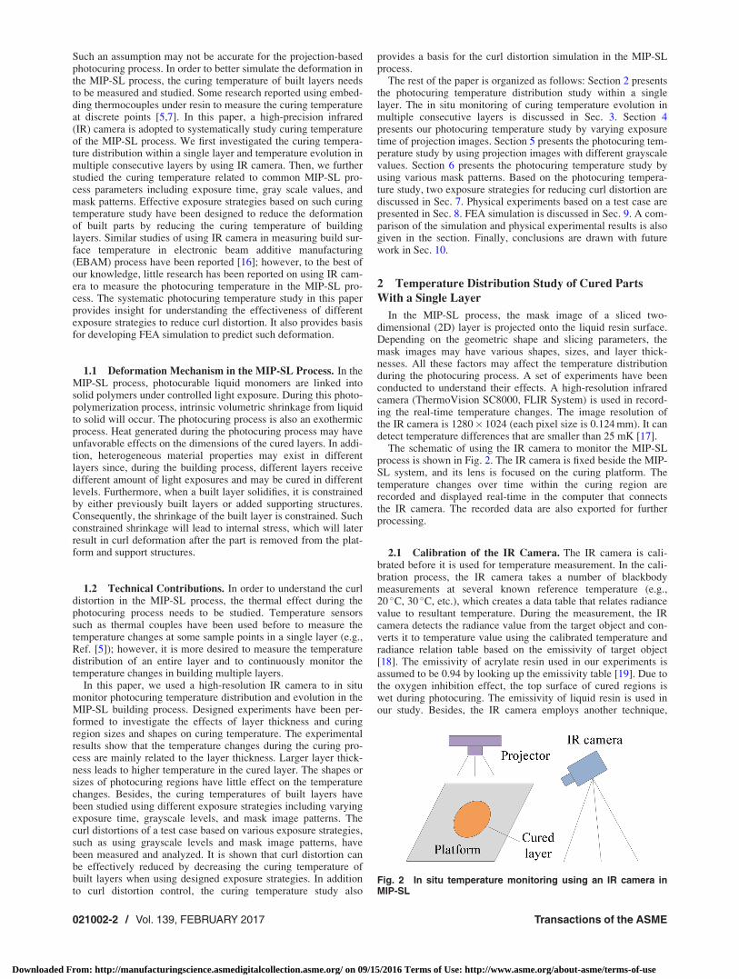
2.3 Temperature Distribution. After finishing the physicalexperiments, the temperature data recorded by the IR camera areexported to excel files and then processed by a MATLAB program.Figure 4(a) shows the maximum temperatures when building acircle with R¼ 3 in. The figure shows that the temperature distri-bution within the curing region is nonuniform. The center portionhas lower temperatures than the other portions. The temperaturerange is between 28.5 and 34 �C. Figure 4(b) shows the

temperature distribution along the X axis through the circle center.In the figure, the Y axis denotes the temperature range (in �C),and the X axis is the distance from the circle center (in in.). Thedifferences between the highest and lowest temperature regionsare around 4 �C. The reason for such temperature differences isinvestigated and discussed as follows.

2.4 The Effect of Layer Thickness. In order to understandthe nonuniform temperature distribution within a cured layer, thethickness of the built layer is measured using a digital caliper thathas a measurement resolution of 1 lm. Sampling points from dif-ferent regions in the layer are measured. Figure 4(c) shows thereadings of the layer thickness in some sampling points (in lm).The measurements show that the thickness of the built layer variesranging from 50 lm to 140 lm. Initially, the target layer thicknessis set to be 100 lm; however, due to the surface tension of liquidresin and the limitations of our hardware setup, liquid resin is notspread out uniformly at exactly 100 lm thickness.

The thickness measurement data are then oriented to be alignedwith the temperature distribution image. It shows that the meas-ured thickness distribution matches well to the maximum temper-ature distribution. That is, the higher temperatures occur at thepositions where the layer thicknesses are larger. The same resultshave been found in the remaining four test cases. The alignmentof layer thickness and temperature is because, in the regions withlarger layer thickness, more resin will be cured by the projectionlight. Consequently, more heat will be generated in the photopoly-merization process, which will then lead to higher temperature inthe region.

2.5 The Effect of Shapes and Sizes. In the experiments, allthe five test cases have been built. Accordingly, the temperaturedistributions during the building process are recorded. Some of

Fig. 3 The one-layer experimental design and the test cases

Fig. 4 The temperature distribution and layer thickness of the one-layer circle with R 5 3 in:(a) maximum curing temperature in IR image, (b) temperature distribution along the centerline(top), and physical built layer (bottom), and (c) layer thicknesses measured on selected sam-ple points

Journal of Manufacturing Science and Engineering FEBRUARY 2017, Vol. 139 / 021002-3

Downloaded From: http://manufacturingscience.asmedigitalcollection.asme.org/ on 09/15/2016 Terms of Use: http://www.asme.org/about-asme/terms-of-use

the sample points in the same positions on the platform areselected from each of the five test cases and compared with eachother. The temperature differences between different shapes andsizes are shown in Fig. 5. In the figure, the thermal images of thesefive test cases are compared by calculating their temperature differ-ences in the overlapping regions. The temperature differences atdifferent positions are represented in grayscale images. The smallerthe temperature difference is, the darker the image is. As shown inFig. 5, the overlapping areas of these comparing shapes are nearlyblack, which means the temperature difference in such regions isvery small even they are cured in different shapes and sizes.

In summary, our experimental results show that the temperaturedistribution in the MIP-SL process is mainly related to the layerthickness of the built layer and is less dependent on the particularshape or size of a built layer. This is because the energy generatedby the photopolymerization process plays a major role in tempera-ture increase. It is orders of magnitude larger than the energyinput of the projection light.

3 In Situ Monitoring of Temperature Evolution in

MIP-SL

After getting the basic understanding of the temperature distri-bution within one layer of a built part, the IR camera is used to insitu monitor the entire building process to understand how

temperature evolves in successive layers during the building pro-cess. Since the IR camera cannot see through a glass cover, it isdifficult to use an IR camera to measure the temperature changesin the constrained-surface-based MIP-SL process [1]. In our study,we constructed a setup based on the free-surface-based MIP-SLprocess to facilitate the IR camera measurement. That is, insteadof using a glass cover to recoat liquid resin, a blade is used in thesystem to form thin layers of liquid resin. To recoat a layer, theblade sweeps through the platform to remove excessive resin onthe previously built layers.

Figure 6 shows our setup of using the IR camera to monitor thefree-surface-based MIP-SL process. The IR camera is fixed on atripod that can be adjusted to gain a proper view of photocuringregions. The IR camera is connected to a computer using a cablesuch that the temperature data can be transferred and recorded.When the building process starts, real-time temperature readingscan be obtained on selected points of the photocuring regions.

3.1 Experimental Design. A set of experiments weredesigned to investigate how photocuring temperature evolves inconsecutive layers, and how building parameters like layer dimen-sion and layer thickness may affect temperature changes in thebuilding process. A rectangular thin part as shown in Fig. 1 hasobvious curl distortion. The similar shape is used in our study.Rectangular bars with different sizes and layer thicknesses arebuilt in our MIP-SL setup and monitored by the IR camera.Table 1 shows the dimensions and building parameters of the fourtest cases. The schematic dimensions of test #1 are shown inFig. 7.

All the test cases are built directly on the platform withoutusing any support structures. For each test case, four samplepoints are picked inside a photocuring region to show the temper-ature variance within the region. Figure 8(a) shows the four sam-pling points and their positions related to the photocuring regionof a sliced rectangle. During the building process, both the meanand maximum temperatures within the curing region are recorded.

3.2 Temperature Evolution in Consecutive Layers. Figure 8(b)shows the temperature plot for cursor 1 in test case #1. It can beobserved that the maximum temperature in building the first tenlayers is �31.5 �C, which is measured at the tenth layer.In comparison, the resin temperature is measured at 24.7 �C.The maximum temperature of each layer is gradually increasing.

Fig. 5 The temperature differences between overlapping areas of five test cases: (a) circles of R 5 2 in. and R 5 3 in., (b)circles of R 5 1 in. and R 5 2 in., (c) circle of R 5 1 in. and square of L 5 2 in., and (d) squares of L 5 2 in. and L 5 3 in.

Fig. 6 Using an IR camera to in situ monitor the free-surface-based MIP-SL process

Table 1 Dimensions and building parameters of four test cases

Test case # Width (mm) Length (mm) Thickness (mm) Layer thickness (mm) Exposure time (s)

1 5 60 1.27 0.127 242 8 60 1.27 0.127 243 10 60 1.27 0.127 244 5 60 1.27 0.254 36

021002-4 / Vol. 139, FEBRUARY 2017 Transactions of the ASME

Downloaded From: http://manufacturingscience.asmedigitalcollection.asme.org/ on 09/15/2016 Terms of Use: http://www.asme.org/about-asme/terms-of-use

This may be caused by the following reasons. The thermal conduc-tivity of the cured resin is low. Therefore, the heat generated duringthe curing process is dissipating slowly. The current layer is curedon the top of previous layers, which may have a higher temperaturethan liquid resin especially when the exposure time for each layer isshort (e.g., 24 s). However, the temperature increase rate is becom-ing smaller as more layers are built. For example, the maximumtemperature increases 1 �C from the second to the third layer; incomparison, the maximum temperature increases only 0.2 �C fromthe ninth to the tenth layer. It suggests that the maximum tempera-ture is getting stable as more layers have been built. The curing tem-perature is the result of three factors: overcure effect, initialtemperature condition for the layer, and heat transfer to the environ-ment. For the first few layers, more heat is generated for each layerprimarily due to the overcure effect, in which light can penetratemultiple layers and cause additional curing. For the later layers, theovercure effect is smaller and becomes stable, while more heat istransferred to the environment compared to the earlier layers due totemperature gradient (i.e., temperature is higher). Therefore, theincrease rate is becoming smaller and approaching stable.

The temperature plot also shows that the maximum temperaturein the first layer is higher than that in the second layer. This is dueto the overcuring effect that exists in the MIP-SL process. That is,the light exposure of a layer is designed to cure 2–3 layers belowin order to bond neighboring layers well. From our previousexperiments base on a single layer, it is observed that the tempera-ture increase is directly related to the layer thickness of liquidresin. The larger layer thickness leads to a higher temperatureincrease. The cured resin in the first layer may be thicker due tothe overcuring effect.

3.3 One Building Cycle Analysis. Figure 9 shows the build-ing sequence of building one layer using our experimental MIP-SL system. First, the platform moves down below the liquid resinsurface. The blade moves back to its beginning position. The plat-form then moves up to leave a gap of one-layer thickness. The

blade sweeps across the platform to remove excess resin. Finally,after a uniform thin layer of liquid resin has been prepared, amask image is projected using the DMD system to expose the liq-uid resin for a specified time.

Corresponding to the building sequence, the temperature evolu-tion in one building cycle is shown in Fig. 10. Along the X axis ofthe figure, t1 corresponds to the time when the platform startsmoving down below the liquid surface; t2 is the time when theblade starts sweeping right; t3 is the time when the blade startssweeping left; and t4 is the time when the projection light isturned on. The time as shown in Fig. 10 is in seconds. It takes�10 s for the blade to sweep from left to the right of the platform.In comparison, the light exposure time of fully curing a layer is24 s. It is shown in Fig. 10 that the temperature at the measuredpoint drops quickly when the platform moves down. The tempera-ture increases slowly in the beginning of light exposure since ittakes some time to dissolve the oxygen in the liquid resin that pre-vents curing. However, after the curing process starts, the temper-ature increases rapidly until it rises to the maximum temperature.

3.4 Temperature Variation Study Within One Layer. Thetemperature evolutions of the four sample points in test case #1are shown in Fig. 11. It can be observed that the trends of temper-ature increase at these four points are similar. Cursor 1 has slightly

Fig. 7 Dimensions of a built part (in mm)

Fig. 8 Four sample points in a photocuring region and the temperature plot at cursor 1 for test case #1

Fig. 9 Building sequence in MIP-SLA

Journal of Manufacturing Science and Engineering FEBRUARY 2017, Vol. 139 / 021002-5

Downloaded From: http://manufacturingscience.asmedigitalcollection.asme.org/ on 09/15/2016 Terms of Use: http://www.asme.org/about-asme/terms-of-use

higher temperatures than the other three sample points. The reasonis that cursor 1 is located at the position that is closest to the rightboundary of the platform. Note that the layer recoating in oursetup is done by sweeping the blade from the right side to the leftside of the platform. Therefore, cursor 1 will be recoated first.Due to liquid viscosity, it is observed that there will be some left-over resin on the right boundary portion of a built region, whichwill make the right portion where cursor 1 is located slightlythicker. Consequently, cursor 1 will have a higher temperatureduring the photocuring process. The other three sample points,cursors 2–4, have very close temperature measurements (as can beseen in dashed, dashed–dotted, and dotted curves). The maximumtemperature difference between these points in the building pro-cess is less than 0.2 �C.

3.5 Verification of the Effects of Layer Size and Thicknesson Temperature. Test cases #1, #2, and #3 have the same dimen-sions and building parameters on their length (60 mm), thickness(1.27 mm), layer thickness (0.127 mm), and exposure time (24 s).Only their widths are different (i.e., 5 mm, 8 mm, and 10 mm).The mean temperatures within the cured layers of these threetest cases are shown in Fig. 12(a). It can be observed that themean temperatures for these three test cases are close, withthe maximum temperature difference around 1 �C. The meantemperature profiles for test case #1 (5� 60� 1.27 mm) and #3(10� 60� 1.27 mm) almost overlap with each other, with themaximum temperature difference less than 0.3 �C. This confirmsour previous experimental result that the temperature increase of acured layer is not dependent on its shape and size.

For test case #2 (8� 60� 1.27 mm), there is a slight tempera-ture deviation from the other two test cases. However, after care-ful examination, it can be observed that the deviation mainlycomes from the first two layers. From the third to tenth layer, thetemperature increase rates for the three test cases are close. Thereason for the temperature deviation in the first two layers may bedue to inaccurate leveling of liquid resin; hence, thinner liquidlayers are formed in the beginning of the building process in testcase #2.

Test case #4 has the same part sizes as test case #1; however, ituses a layer thickness of 0.254 mm instead of 0.127 mm that isused in the other three test cases. Accordingly, the exposure timefor each layer is increased from 24 s to 36 s. A comparison of themean temperature in test cases #1 and #4 is shown in Fig. 12(b).It is shown that the highest mean temperature in test case #4 isclose to 32.7 �C, while it is around 30.1 �C in test case #1. This ismainly due to a larger layer thickness used in the building process.

Fig. 10 Temperature plot of a building cycle at cursor 1

Fig. 11 Temperature evolutions at four and three sampling points

Fig. 12 Mean temperature plots of the test cases with (a) different widths and (b) different thicknesses

021002-6 / Vol. 139, FEBRUARY 2017 Transactions of the ASME

Downloaded From: http://manufacturingscience.asmedigitalcollection.asme.org/ on 09/15/2016 Terms of Use: http://www.asme.org/about-asme/terms-of-use

Similar to the other three test cases, the temperature increase ratefor test case #4 is getting smaller as more layers are built.

Based on the temperature evolution measurement results forbuilding multiple layers, the following conclusions can be drawnfor the MIP-SL process:

(1) The temperature increase is not dependent on the shapesand sizes of the cured regions.

(2) The temperature increase is mainly related to the layerthickness of a cured layer. The larger the layer thickness,the higher the temperature it will reach.

(3) For test parts built directly on platform, the temperature ineach layer is getting higher as more layers are built; how-ever, the temperature increase rate is becoming smallerafter a few layers.

4 Photocuring Temperature by Varying Exposure

Time

Exposure time is a critical building parameter in the MIP-SLprocess. Longer exposure time can provide more energy to bettersolidify liquid resin in the building process. Since heat will begenerated when liquid resin solidifies, longer exposure time mayresult in higher temperature in the cured layers. The relationshipbetween exposure time and the maximum photocuring tempera-ture is studied in the section.

4.1 Experiment Design. In our study to understand how cur-ing temperature is related to exposure time, ten different levels ofexposure time (5 s, 10 s, 15 s, 20 s, 25 s, 30 s, 35 s, 40 s, 45 s, and50 s) are tested. The workflow of our experiments is shown inFig. 13. The experiments are conducted using a free-surface MIP-SL setup as shown in Fig. 6. The size of the test layers is5 mm� 60 mm. and the layer thickness is 0.127 mm. In theexperiments, ten layers are first built on the platform to form thebase on which the test layers will be built. The added base can

also eliminate the effect of unevenness of the platform if any.Subsequent test layers are built on the base layers or previouslybuilt test layers. Before a test layer is built, the platform movesdown to submerge the built layers in liquid resin and remainsthere for over 3 min until the previously built layers cool down.After the platform moves up, the blade of the system sweepsacross the platform to prepare a thin layer of liquid resin. Whenprojection light is turned on to expose the photocuring region fora specified exposure time (e.g., 5 s, 10 s, etc.), the IR camera startsrecording the temperature evolution at the same time. The record-ing time is set to be 90 s to capture the whole cycle of temperatureevolution. After testing with specified exposure time, the test layeris then exposed to the projection image with an additional 2 minto make it fully cured. The same IR camera is used to record thisfully photocuring process for 3 min. (The IR camera settings arethe same as those used in the previous step of recording the 90 sexposing process.) The aforementioned process is repeated forbuilding the next layer. The experiment workflow is designed toeliminate the effects of other factors on the photocuring tempera-ture of test layers, e.g., the accumulation of heat from previoustest layers, or the variation of different runs of experiments.

4.2 Exposure Time Effect on Photocuring Temperature.The temperature measurement view using the IR camera is shownin Fig. 8(a), in which polygon 2 is the entire curing region of thetest layers. Hence, the average curing temperature of the layer iscalculated based on the measured temperatures of all the pixelsthat lie within the polygon. The photocuring temperatures arerecorded and viewed in real-time through a control software sys-tem. As shown in Fig. 13, an additional fully curing process isconducted after exposing a test layer for a certain time to ensureall the liquid resins of the layer have been cured.

4.2.1 Exposure Time of 5 s. The average temperature of thetest layer using the exposure time of 5 s is plotted in solid curve inFig. 14. The average temperature in the corresponding fully pho-tocuring process using additional 2 min exposure is plotted indashed curve in Fig. 14. It can be observed that the temperatureincrease in the solid curve is very small (from 25.3 �C to 25.4 �C),and the maximum temperature is measured at the end of lightexposure. However, the maximum temperature increase in thefully curing process (the dashed curve) is large. It takes almost30 s for the layer to reach the maximum temperature (�28.7 �C).Then, the layer’s temperature begins to drop even though the layeris still under the light exposure. The light exposure of the fullyphotocuring process ends at the time t¼ 123 s. After that, the tem-perature cools down much faster compared to when the lightexposure is on.

4.2.2 Exposure Time of 15 s. The temperature evolution dur-ing the curing process using exposure time of 15 s and correspond-ing fully curing process are shown as the dotted curve and dottedcurve with triangle markers, respectively, in Fig. 14. The dottedcurve shows that the exposure starts at time t¼ 8 s, and the maxi-mum temperature during the curing process is 27.7 �C, which ismeasured at the end of the light exposure (t¼ 23 s). It can also beseen that the photocuring temperature rises very slowly (from25.4 �C to 25.5 �C) for the first 5 s (t¼ 8–13 s), and it then risesrapidly (from 25.4 �C to 27.7 �C) in the next 10 s under the lightexposure (t¼ 13–23 s). The temperature cools down when lightexposure ends; however, the cool rate drops as time passes. Themaximum temperature during the fully photocuring process is�28 �C. Similar to the result observed when using exposure timeof 5 s, the cool rate after the light exposure ends is faster thanwhen the light exposure is on.

4.2.3 Exposure Time of 45 s. The temperature plots during thephotocuring process using the exposure time of 45 s and therelated fully curing process are shown as the solid curve withcircle markers and dotted curve with square markers in Fig. 14,respectively. The maximum temperature during the curing process

Fig. 13 Workflow of testing various exposure times on themaximum curing temperature

Journal of Manufacturing Science and Engineering FEBRUARY 2017, Vol. 139 / 021002-7

Downloaded From: http://manufacturingscience.asmedigitalcollection.asme.org/ on 09/15/2016 Terms of Use: http://www.asme.org/about-asme/terms-of-use

is 28.3 �C; and the maximum temperature during the fully photo-curing process is 26.5 �C. The light exposure starts at t¼ 7 s andends at t¼ 52 s. The maximum temperature is measured att¼ 36 s, which is before the light exposure ends. The relationshipbetween the curing temperature and the exposure time can bedrawn as follows. For the first 5 s exposure, the layer temperaturerises slightly, which may be due to the oxygen inhibition effect[21]. For the next 24 s exposure, the temperature rises rapidly toreach the maximum; however, the increasing rate slows down.After reaching the maximum, the temperature drops even thoughit is still under the light exposure.

The temperature plots during the curing process based on otherexposure times (10 s, 20 s, 25 s, 30 s, 35 s, 40 s, and 50 s) and thecorresponding fully photocuring process have similar trends asthose of using 45 s. The maximum temperatures using these tenexposure time settings are shown in Table 2 and plotted inFig. 15. As can be seen in Fig. 15, the curing temperature rises asthe exposure time increases. The curing temperature reaches themaximum when the exposure time is around 30 s. In the fully pho-tocuring process, the maximum photocuring temperaturedecreases as longer exposure time is applied in the previous expo-sure process. This is because a larger portion of the test layer hasbeen cured when the exposure time is increased. Thus, less liquidresin remains in the layers to be cured in the fully photocuringprocess.

5 Curing Temperature by Varying Grayscale Values

Mask image exposure based on different grayscale values couldbe an effective way of controlling the exposure energy since dif-ferent grayscale values correspond to different energy intensities[22]. The relationship between grayscale values and related photo-curing temperature is investigated in the section.

The maximum and the minimum light intensities of a maskimage for a DMD device are 255 and 0, respectively. Amongthem, eight levels of grayscale values, specifically, 70, 100, 130,160, 190, 205, 220, and 255, are studied. Some grayscale maskimage examples are shown in Fig. 16. The workflow of the experi-ments is similar to the one as shown in Fig. 13 for testing variousexposure times. The only difference is that, instead of exposing

the test layer using the maximum light intensity (255) with aspecified exposure time, the test layer is exposed using differentgrayscale levels for certain exposure time, which is set to ensurethe photocuring temperature will reach to the maximum.

Fig. 14 Photocuring temperature using different exposure times

Table 2 Comparisons of the exposure time effects

Exposure time (s) 5 10 15 20 25 30 35 40 45 50

Max T during exposure (�C) 25.4 26.6 27.7 28.3 28.4 28.2 28.3 28.3 28.3 28.6Max T during fully curing process (�C) 28.7 28.8 28 27.4 27 26.7 26.6 26.5 26.5 26.3

Fig. 15 Comparisons of the maximum curing temperaturesusing varying exposure time

Fig. 16 Examples of grayscale mask images

021002-8 / Vol. 139, FEBRUARY 2017 Transactions of the ASME

Downloaded From: http://manufacturingscience.asmedigitalcollection.asme.org/ on 09/15/2016 Terms of Use: http://www.asme.org/about-asme/terms-of-use

Experiments are designed to explore the maximum temperaturethat a cured layer can reach using a specific grayscale level. Like-wise, the test layer will be fully cured using the maximum lightintensity (255) for 2 min after the light exposure using a grayscalelevel has been finished.

5.1 Grayscale Level Exposure Study

5.1.1 Grayscale Level of 130. The curing temperature duringthe grayscale exposure process and its corresponding fully curingprocess are plotted in solid and dashed curves, respectively, inFig. 17. The exposure time of using grayscale 130 is chosen to be45 s. It can be seen from the figure that the temperature almoststays the same during the exposing process using grayscale 130,while the maximum temperature during the fully photocuring pro-cess reaches 29 �C. The temperature plot shows that grayscale 130cannot provide enough energy to cure liquid resin (i.e., the inputenergy is less than the critical energy of the liquid resin). The tem-perature plot of the fully photocuring process is very similar to theones of testing different exposure times in Sec. 4.

5.1.2 Other Grayscale Levels. The curing temperature plotsduring the exposure process using the grayscale levels of 160,190, and 220 are also shown in Fig. 17. The maximum tempera-ture is around 26.7 �C when using grayscale 160 with a total expo-sure time of 150 s (shown in dotted curve). The temperatureevolution is similar to the ones in Sec. 4; however, temperatureincrease rate is much smaller. The light exposure starts at t¼ 8 s,and ends at t¼ 158 s. The temperature rises little from t¼ 8 s tot¼ 33 s. In this paper, this period is denoted as the oxygen inhibi-tion period. The temperature reaches the maximum at t¼ 117 s.That is, it takes 109 s of exposure using grayscale 160 to reach themaximum temperature. The dotted curve with circle markersdenotes the temperature evolution during the exposure process ofusing grayscale 190 with the exposure time of 90 s. The maximumtemperature reaches 27.3 �C at t¼ 65 s. The light exposure startsat t¼ 5 s, and the oxygen inhibition period lasts 16 s. The maxi-mum temperature of using grayscale 220 reaches 28.1 �C att¼ 45 s, as denoted by solid curve with circle markers. The totallight exposure time is 90 s, which starts at t¼ 9 s. The oxygeninhibition period lasts 6 s, which is shorter than the ones usinglower grayscale levels.

The maximum photocuring temperatures based on differentgrayscale levels are shown in Table 3 and plotted in Fig. 18. It canbe seen that the maximum photocuring temperature increases asthe grayscale level increases. Since a higher level of grayscalelevel corresponds to higher energy input, the related curing pro-cess will be faster. A lower grayscale level can slow down thephotocuring process, which lead to a lower maximum

temperature. Also, the maximum temperature drops in the fullyphotocuring process when the layer uses a higher grayscale levelin the curing process.

The time it takes to reach the maximum temperature, as well asthe oxygen inhibition period, is also shown in Table 3. Both of thetime is plotted in Fig. 19. It shows that, as the grayscale levelbecomes higher, the oxygen inhibition period and the time to reachthe maximum temperature decrease. This is because a higher gray-scale level provides higher energy for photocuring liquid resin.

6 Curing Temperatures by Using Mask Patterns

Instead of exposing the whole area of a layer at the same time,the layer can be divided into several smaller regions, and eachregion can be exposed at different times. These smaller regionsare denoted as mask patterns [12]. Since the temperature is mainlyrelated to the layer thickness, the temperature of a small regionduring the curing process is almost the same as the one when thewhole region is exposed. However, the thermal cooling and

Fig. 17 Photocuring temperature using different grayscale levels exposures

Table 3 Comparisons of the grayscale exposure effect

Grayscale (0–255) 70 100 130 160 190 205 220 255

Max T during exposure (�C) 25.3 25.5 25.6 26.7 27.3 27.6 28.1 28.6Max T during fully curingprocess (�C)

29 28.7 29 27.4 26.9 26.7 26.7 26.4

Oxygen inhibition period (s) — — — 25 16 13 6 5Time to reach maximum T (s) — — — 109 60 58 36 30

Fig. 18 Grayscale effects on curing temperature

Journal of Manufacturing Science and Engineering FEBRUARY 2017, Vol. 139 / 021002-9

Downloaded From: http://manufacturingscience.asmedigitalcollection.asme.org/ on 09/15/2016 Terms of Use: http://www.asme.org/about-asme/terms-of-use

polymerization shrinkage will only affect the local discreteregions. The final accuracy of the built layer will be less affectedby the temperature increase and related shrinkage of these smallregions since they are not connected with each other.

In this paper, the curing temperatures of the cured layers using aset of mask patterns are investigated. The schematics of the maskpatterns studied in our experiments are shown in Figs. 20(a) and20(b). In comparison, Fig. 20(c) shows the mask image of the entirelayer without applying any patterns. In the mask images, the whiteareas denote the regions to be cured under the light exposure, whilethe black regions receive no light exposure. In mask pattern 1, a gap

size of three pixels is designed to separate the large curing regioninto smaller regions. Mask pattern 2 exposes the gap regions that areleft to be uncured after applying mask pattern 1. These two maskpatterns will be applied sequentially with specified exposure time.The whole region will then be fully cured after applying the twomask patterns, similar to using a single mask exposure for the entireregion as shown in Fig. 20(c). A difference between applying maskpatterns and without lies in the curing temperature of built layers.After using mask patterns, the curing temperature of the built layersmay be lower than those without mask patterns.

6.1 Curing Temperature Study. Mask patterns 1 and 2 asshown in Fig. 20 are used to investigate the related maximum pho-tocuring temperatures in the built layers. The workflow of experi-ments is similar to Fig. 13. Instead of exposing the whole regionof a test layer, different small regions are exposed by using thesetwo patterns, each with a specified exposure time. Eight differentlevels of exposure time (i.e., 10 s, 15 s, 20 s, 25 s, 30 s, 35 s, 40 s,and 45 s) are tested. The average temperature within the wholeregion of a built layer is measured and plotted. Two examples ofthe curing temperatures are shown in Fig. 21, in which the temper-atures during the photocuring process are plotted. The three crestsof the plotted curves correspond to exposing the two mask pat-terns and the fully photocuring process over time.

The curing temperature evolution of the first test case is shownin solid curve in Fig. 21, in which each of the two mask patterns isapplied to expose 25 s, and the layer is then fully cured using themask image of the entire region for a long time. The average tem-perature of the test layer during the two patterns exposure and thefully cured process is around 26 �C. In comparison, the maximumtemperature rises to 26.6 �C when applying the first mask patternwith exposure time of 40 s, as shown in dotted curve, and it dropsto 26.2 �C and 25.9 �C during the second mask pattern exposureand the fully curing process, respectively.

Table 4 shows the maximum temperature during the fully curingprocess after using mask patterns for different exposure times. It canbe observed that, when the mask pattern exposure increases, themaximum temperature during the fully curing process decreases.This is because small regions within the test layer have been par-tially cured during the mask pattern exposure, and the ratio of curingregions increases as the exposure time becomes longer. Thus, lessliquid resin will need to be cured during the fully curing process.

7 Photocuring Strategies of MIP-SL for Curl

Distortion Control

It is desired to have a smaller temperature difference betweenthe maximum curing temperature and the room temperature

Fig. 19 Grayscale effects on curing time

Fig. 20 Mask images of (a) mask pattern 1, (b) mask pattern 2,and (c) entire region

Fig. 21 Photocuring temperature using mask patterns with different exposure times

021002-10 / Vol. 139, FEBRUARY 2017 Transactions of the ASME

Downloaded From: http://manufacturingscience.asmedigitalcollection.asme.org/ on 09/15/2016 Terms of Use: http://www.asme.org/about-asme/terms-of-use

during the curing process since the curl distortion is related to theincreased curing temperature of each layer. Based on our previousstudy on varying exposure time, grayscale levels, and mask pat-terns, two exposure strategies have been developed with the aimof reducing the maximum curing temperature difference andrelated curl distortion of built parts. Note that a disadvantage ofusing these strategies, compared to the single exposure of a wholelayer, is a longer building time that is required. This is a tradeoffto be made in order to reduce the curl distortion. How to balancethe fabrication speed and the curl distortion needs to be furtherinvestigated in the future.

7.1 Photocuring Strategy Using Grayscale Exposure. Asshown in Fig. 17, grayscale level 190 can make the maximum cur-ing temperature during the grayscale exposure process and thefully curing process close to each other, which stays around 27 �C.Thus, the exposure strategies based on grayscale 190 may be ableto reduce the maximum photocuring temperature difference ofbuilt layers and, consequently, reduce the curl distortion of thebuilt part.

An exposure strategy based on grayscale 190 is to expose amask image using grayscale 190 for 80 s, and then to use gray-scale 255 to expose the layer for 30 s. The curing temperature dur-ing building a test part can be recorded using the IR camera. Theresulting temperature plot of a test part with 22 layers is shown inFig. 22, in which the dotted curve records the liquid resin temper-ature while the solid curve represents the temperature of the builtlayers. The first four layers are the base layers, and the followingeight layers are supports. The remaining ten layers are the builtlayers related to the given part, which will be applied with theexposure strategy. Hence, the curing temperature of the last tenlayers is what we are interested in. It can be seen from the temper-ature plot (solid curve) that the maximum temperatures of the lastten layers are rather close to each other, which is about 2.8 �Chigher than the temperature of liquid resin (dotted curve). In com-parison, the curing temperature plot for the same test part usinggrayscale 255 to expose the whole layer for 40 s is shown in Fig.23. The maximum temperature of the last ten layers is about4.3 �C higher than the temperature of liquid resin. The

temperature increase is also higher than that of using the grayscaleexposure as shown in Fig. 22.

7.2 Photocuring Strategy Using Mask Pattern Exposure.As shown in the mask patterns exposure study (refer to Sec. 6),the curing temperature of test layers can be reduced by applyingmask patterns, since a portion of liquid resin in a layer is cured ata time during the mask pattern exposure. Thus, the mask patternexposure may effectively reduce the curl distortion of built parts.The temperature plot of using the mask pattern exposure strategyis shown in Fig. 24. In each of the last ten layers, mask pattern 1as shown in Fig. 20(a) is first applied for 18 s; mask pattern 2 asshown in Fig. 20(b) is then applied for 12 s; finally, the wholeregion is exposed using the mask image as shown in Fig. 20(c) for20 s. The temperature plot as shown in Fig. 24 shows that themaximum temperature of the last ten layers is �3.4 �C higher thanthe temperature of liquid resin.

8 Physical Experiments and Results

A rectangular thin part based on the two aforementioned expo-sure strategies is built using the MIP-SL setup as shown in Fig. 6and monitored by the IR camera. The schematic dimension of thetest part is shown in Fig. 7. The layer thickness is 0.127 mm(0.005 in.), and the test part has a total of ten layers. Before build-ing the part, anchor supports with a height of 1 mm are added onthe bottom of the part for the easy removal of the part after thebuilding process. Accordingly, the test part is built on eight layersof the supports, which fix the part on the platform.

8.1 Physical Experiments. The two exposure strategies areapplied to investigate their effects on the curl distortion in thebuilt parts.

(1) The first exposure strategy is based on grayscale exposure,in which (i) each layer is first exposed using grayscale 255for 5 s (to overcome the oxygen inhibition effect); (ii) thelayer is then exposed using grayscale 190 for 60 s; and (iii)finally, the layer is exposed using grayscale 255 for 10 s.

(2) The second exposure strategy is based on mask patternexposure, in which (i) each layer is first exposed usinggrayscale 255 for 5 s; (ii) the layer is then exposed usingmask patterns similar to those shown in Figs. 20(a) and20(b). A small modification is to expose the layer boundaryseparately from the inner regions (refer to a layer exampleas shown in Fig. 25). Each of the three patterns will beexposed for 25 s; (iii) finally, the layer is exposed usinggrayscale 255 for 10 s.

Table 4 The maximum temperature in the fully curing processafter applying mask patterns

Exposure time of mask pattern 10 15 20 25 30 35 40 45

Maximum temperature (�C) 28.2 27.7 27.1 26.1 25.8 26 25.9 25.9

Fig. 22 Curing temperature of using grayscale 190

Journal of Manufacturing Science and Engineering FEBRUARY 2017, Vol. 139 / 021002-11

Downloaded From: http://manufacturingscience.asmedigitalcollection.asme.org/ on 09/15/2016 Terms of Use: http://www.asme.org/about-asme/terms-of-use

To study the effect of these two exposure strategies on curl dis-tortion, a baseline part has also been built using a single exposure(i.e., exposing the whole region of a layer using grayscale 255 for40 s). To reduce the effect of the boundary layers, the first and thelast layers of all the test parts are built with the single exposurestrategy. The remaining layers of the test parts are built using theaforementioned grayscale exposure strategy, the mask patternexposure strategy, and the single exposure strategy, respectively.

8.2 Experimental Results. After the building process, thebuilt parts are removed and cleaned. The measurement of thebuild parts is conducted based on the schematic measurement as

shown in Fig. 26. The curl distortion of the parts is denoted by thesize of e. A precision measurement machine from Micro-Vu [23]is used in measuring each built part. The measurement procedureis described in more detail in Ref. [24].

The experimental results of the measured e values are shown inTable 5. Each of the test cases is repeated four times, and the aver-age curl distortion is calculated. As shown in the table, the aver-age curl distortion for the baseline parts is 0.431 mm; incomparison, the curl distortions for the test parts using the gray-scale and mask pattern exposure strategies are 0.232 mm and0.26 mm, respectively. The physical experiment results show thatthe two exposure strategies using grayscale values and mask pat-terns are effective in reducing the curl distortions in the MIP-SLprocess (�40% reduction).

Fig. 24 Curing temperature of mask pattern exposure

Fig. 25 Exposure strategy using mask patterns Fig. 26 Schematic of curl distortion measurement

Fig. 23 Curing temperature of grayscale 255 for 40 s

021002-12 / Vol. 139, FEBRUARY 2017 Transactions of the ASME

Downloaded From: http://manufacturingscience.asmedigitalcollection.asme.org/ on 09/15/2016 Terms of Use: http://www.asme.org/about-asme/terms-of-use

9 Simulation

Based on the curing temperature study in the MIP-SL process,we investigate the possibility of simulating the curl distortion ofbuilt parts based on the observed thermal effect. A finite-elementanalysis (FEA) software package, COMSOL MULTIPHYSICS, is adoptedto simulate the building process. A structural mechanics model isused to incorporate the thermal shrinkage effect. A linear elasticmaterial model with constant Young’s modulus, Poisson’s ratio,and coefficient of thermal expansion is assumed to simplify thesimulation process. Test parts with dimensions 5� 60� 1.27 mmand layer thickness of 0.127 mm as shown in Fig. 7 are simulatedusing COMSOL.

9.1 Modeling of the Layer-Based MIP-SL Process. In theMIP-SL process, a part is built on a layer-by-layer sequence. Tosimulate this layer-based dynamic building process, a techniquecalled birth and death method has been applied. The method wasalso used to simulate fusion deposition modeling (FDM) and otherdynamic processes before [25,26]. In this method, each layer isactivated when it is being exposed in current step. For example,only the first layer will be activated in the first building step; andthe second layer will be activated in the second building step.Note that, in the second building step, the first layer is still activewhile all the above layers are deactivated. To deactivate a layer,its Young’s modulus is set to a very small value (e.g.,1� 10�12 Pa). Thus, the deactivated layers will have negligiblestress. When the layer is activated, its Young’s modulus is set to anormal value (e.g., 2.68� 109 Pa). In the newly activated layer,phase change from liquid to solid takes place. After the photocur-ing process, its temperature will decrease from its maximum tem-perature to room temperature. The temperature drop will lead toshrinkage of the layer and related internal thermal stress due tothe external constraints in the building process.

In the simulation of test part with ten layers, a total of 11 stepshave been conducted. The first ten steps calculate the initial stressfrom the currently activated layers. The last step (11th) calculatesthe total stresses generated from the building process of the tenlayers. The final distortion can then be calculated after the releaseof these stresses during the part removal process.

9.2 FEA Model Settings and Simulation Results. Thegeometry model of the ten layers is first built. Due to the symme-try along the X and Y axes, only 1/4 of original size was modeled.Tetrahedron mesh elements are used to mesh the part. All thelayers are meshed such that each mesh element and node has auniform index. Table 6 shows the material properties used in thesimulation. It is assumed that the material properties are constantin building each layer. The property values are based on previousresearch [9] and open sources [27,28].

Two kinds of mechanical boundary conditions were applied inthe simulation. They are:

(a) The constraint of fixing the first layer: The bottom surfaceof the first layer is fixed during the building of the tenlayers. After the building process, the part is removed fromthe platform. Hence, the bottom constraint added to the firstlayer can then be removed to let the ten-layer part to

deform freely under the residual stress that is generated inthe building process.

(b) The constraint of symmetric boundary: Since the part issymmetric in the X and Y axes, the symmetric boundaryconditions are applied to the 1=4th of the built part to reducethe computation cost. The symmetric boundary conditionsare applied in both the building process and part removalprocess.

When a layer is cured, its temperature drops from the maximumtemperature to the room temperature, which will cause shrinkagein the cured layer. The temperature drop is modeled as thermalload in the mechanical structural analysis. In the simulation, thereference temperature is set to the measured results for each layerwhen it is activated. From the IR camera temperature measure-ment, the maximum curing temperature of test layers in baselinepart is about 4.3 �C than liquid resin temperature. This tempera-ture differences for test parts using the grayscale and mask patternexposures are around 2.8 �C and 3.4 �C, respectively. These tem-peratures are incorporated in the FEA model.

The simulation result of the baseline part is shown in Fig. 27.Coefficient of thermal expansion is set to 0.4� 10�4 1/K. The curldistortion is 0.221 mm. The curl distortion of the test parts usingthe grayscale and mask pattern exposure is 0.139 mm and0.165 mm, respectively. The simulation results show that the testparts using the designed exposure strategies will have smaller curldistortion than the baseline part, and the curl distortion is relatedto the curing temperature during the building process.

Table 5 Curl distortion of test parts

Curl distortion (mm)

Test parts Replicate 1 Replicate 2 Replicate 3 Replicate 4 Average

Baseline 0.408 0.442 0.434 0.44 0.431Grayscale exposure 0.201 0.279 0.215 0.232 0.232Mask pattern exposure 0.251 0.234 0.243 0.312 0.260

Table 6 Material properties in simulation

Property Value Unit

Young’s modulus 3.2� 109 PaPoisson’s ratio 0.3 —Density 1100 kg/m3

Coefficient of thermal expansion (0.4–1.2)� 10�4 1/K

Fig. 27 Simulation result of baseline part

Journal of Manufacturing Science and Engineering FEBRUARY 2017, Vol. 139 / 021002-13

Downloaded From: http://manufacturingscience.asmedigitalcollection.asme.org/ on 09/15/2016 Terms of Use: http://www.asme.org/about-asme/terms-of-use

When compared with the physical experiment results, the simu-lation results are smaller in all the three test cases. Several reasonsmay account for the differences. One reason is that the polymer-ization shrinkage is not considered in the FEA model. Anotherreason is the boundary condition considered in the current FEAmodel assumes that the bottom of test layers is fully constrained;however, the test part is built on anchor supports, which may havedifferent boundary condition. Besides, the material propertiessuch as coefficient of thermal expansion may need to be calibratedfor the tested liquid resin.

10 Conclusions

The photocuring temperature during the MIP-SL process hasbeen studied using a high-resolution IR camera in this paper. Thephotocuring temperature distribution within a single layer withdifferent sizes and shapes, as well as temperature evolution duringthe building process with multiple consecutive layers, has beeninvestigated. The results show that the photocuring temperature ismainly related to the layer thickness, and larger layer thicknessleads to higher photocuring temperature. Layer sizes or shapeshave little effect on it. Photocuring temperature of built layers isgetting stable as more layers are built in the MIP-SL process.

The effects of varying exposure time, grayscale levels, andmask patterns on the maximum curing temperature have also beenstudied. The results show that the photocuring temperature risesvery little in the beginning of light exposure due to the oxygeninhibition effect. It rises rapidly to the maximum with a decreas-ing rate when reaching the maximum temperature. The curingtemperature can drop even though it is still under light exposure.Accordingly, two exposure strategies have been designed basedon grayscale and mask pattern exposures to reduce the maximumphotocuring temperature of built layers. Test parts using thedeveloped exposure strategies have been built with the curl distor-tion measured. The physical experiments show that the designedexposure strategies can effectively reduce the curl distortionalthough the building time would be significantly longer. TheFEA simulation has also been conducted to verify the physicalexperiments results. The simulation results show similar trends asthe physical experiment measurements with smaller values.

In addition to further exploring better exposure strategies to bal-ance curl distortion and fabrication speed, future work on the FEAsimulation based on the temperature study includes: (1) incorpo-rating the polymerization shrinkage in the FEA model; (2) incor-porating the anchor supports as the constraints in the simulationprocess; and (3) developing a shape compensation method basedon accurate prediction of curl distortion in the MIP-SL process.

Acknowledgment

This work was partially supported by ONR-N00014-11-1-0671.We acknowledge Professor Qiang Huang at USC, and AndrewDavidson, a summer intern from the Brigham Young University,for the help in setting up the IR camera.

References[1] Pan, Y. Y., Zhou, C., and Chen, Y., 2012, “A Fast Mask Projection Stereoli-

thography Process for Fabricating Digital Models in Minutes,” ASME J. Manuf.Sci. Eng., 134(5), p. 051011.

[2] Zhou, C., and Chen, Y., 2012, “Additive Manufacturing Based on OptimizedMask Video Projection for Improved Accuracy and Resolution,” J. Manuf.Processes, 14(2), pp. 107–118.

[3] Tumbleston, J. R., Shirvanyants, D., Ermoshkin, N., Janusziewicz, R., Johnson,A. R., Kelly, D., and Samulski, E. T., 2015, “Continuous Liquid Interface Pro-duction of 3D Objects,” Science, 347(6228), pp. 1349–1352.

[4] Bugeda, G., Cervera, M., Lombera, G., and Onate, E., 1995, “Numerical Analy-sis of Stereolithography Processes Using the Finite Element Method,” RapidPrototyping J., 1(2), pp. 13–23.

[5] Chambers, R. S., Guess, T. R., and Hinnerichs, T. D., 1995, “A Phenomenologi-cal Finite Element Model of Part Building in the Stereolithography Process,”Sandia National Laboratory, Albuquerque, NM, Report No. SAND-94-2565C;CONF-9506149-2.

[6] Huang, Y. M., and Jiang, C. P., 2003, “Curl Distortion Analysis During Photo-polymerisation of Stereolithography Using Dynamic Finite Element Method,”Int. J. Adv. Manuf. Technol., 21(8), pp. 586–595.

[7] Vatani, M., Barazandeh, F., Rahimi, A., and Nezhad, A. S., 2012, “DistortionModeling of SL Parts by Classical Lamination Theory,” Rapid Prototyping J.,18(3), pp. 188–193.

[8] Narahara, H., Tanaka, F., Kishinami, T., Igarashi, S., and Saito, K., 1999,“Reaction Heat Effects on Initial Linear Shrinkage and Deformation in Stereo-lithography,” Rapid Prototyping J., 5(3), pp. 120–128.

[9] Hur, S. S., and Youn, J. R., 1998, “Prediction of the Deformation in Stereoli-thography Products Based on Elastic Thermal Shrinkage,” Polym. Plast. Tech-nol. Eng., 37(4), pp. 539–563.

[10] Tanaka, F., Morooka, M., Kishinami, T., and Narahara, H., 2000,“Thermal Distortion Analysis During Photopolymerization in Stereo-lithography,” 8th International Conference on Rapid Prototyping, Tokyo, Japan,National Taiwan University of Science and Technology, Taipei City, Taiwan,pp. 87–92.

[11] Huang, Y. M., Jeng, J. Y., and Jiang, C. P., 2003, “Increased Accuracy by UsingDynamic Finite Element Method in the Constrain-Surface StereolithographySystem,” J. Mater. Process. Technol., 140(1), pp. 191–196.

[12] Xu, K., and Chen, Y., 2015, “Mask Image Planning for Deformation Control inProjection-Based Stereolithography Process,” ASME J. Manuf. Sci. Eng.,137(3), p. 031014.

[13] Huang, Q., Zhang, J., Sabbaghi, A., and Dasgupta, T., 2015, “Optimal OfflineCompensation of Shape Shrinkage for Three-Dimensional Printing Processes,”IIE Trans., 47(5), pp. 431–441.

[14] Huang, Q., Nouri, H., Xu, K., Chen, Y., Sosina, S., and Dasgupta, T., 2014,“Statistical Predictive Modeling and Compensation of Geometric Deviations ofThree-Dimensional Printed Products,” ASME J. Manuf. Sci. Eng., 136(6),p. 061008.

[15] Huang, Q., 2016, “An Analytical Foundation for Optimal Compensation ofThree-Dimensional Shape Deformation in Additive Manufacturing,” ASME J.Manuf. Sci. Eng., 138(6), p. 061010.

[16] Cheng, B., Price, S., Lydon, J., Cooper, K., and Chou, K., 2014, “OnProcess Temperature in Powder-Bed Electron Beam Additive Manufacturing:Model Development and Validation,” ASME J. Manuf. Sci. Eng., 136(6),p. 061018.

[17] FLIR Systems, 2016, “FLIR SC8000 Series,” FLIR Systems, Inc., Wilson-ville, OR, accessed July 16, 2016, http://www.flir.co.uk/cs/display/?id=53648

[18] FLIR Systems, 2016, “Infrared Handbook,” FLIR Systems, Inc., Wilsonville,OR, accessed July 16, 2016, http://www.flirmedia.com/MMC/THG/Brochures/T559243/T559243_EN.pdf

[19] Electronic Temperature Instruments, Ltd., 2016, “Emissivity Table,” ElectronicTemperature Instruments, Ltd., Worthing, UK, accessed July 16, 2016, http://thermometer.co.uk/img/documents/emissivity_table.pdf

[20] FLIR Systems, 2016, “FLIR X8000sc/X6000sc Series,” FLIR Systems, Inc.,Wilsonville, OR, accessed July 16, 2016, http://www.flir.eu/cs/display/?id=52429

[21] Jariwala, A. S., Schwerzel, R. E., and Rosen, D. W., 2011, “Real-Time Inter-ferometric Monitoring System for Exposure Controlled Projection Lith-ography,” Solid Freeform Fabrication Symposium, pp. 99–110.

[22] Zhou, C., Chen, Y., and Waltz, R. A., 2009, “Optimized Mask Image Pro-jection for Solid Freeform Fabrication,” ASME J. Manuf. Sci. Eng., 131(6),p. 061004.

[23] Micro-Vu Corporation, 2016, “MicroVu Measurement Machine,” Micro-VuCorporation, Windsor, CA, accessed July 16, 2016, http://www.microvu.com/sol.html

[24] Xu, K., and Chen, Y., 2014, “Deformation Control Based on In-Situ Sensors forMask Projection Based Stereolithography,” ASME Paper No. MSEC2014-4055.

[25] Zhang, Y., and Chou, Y. K., 2006, “Three-Dimensional Finite Element Analy-sis Simulations of the Fused Deposition Modelling Process,” Proc. Inst. Mech.Eng., Part B, 220(10), pp. 1663–1671.

[26] Abid, M., Siddique, M., and Mufti, R. A., 2005, “Prediction of WeldingDistortions and Residual Stresses in a Pipe–Flange Joint Using the FiniteElement Technique,” Modell. Simul. Mater. Sci. Eng., 13(3), pp. 455–470.

[27] EnvisionTEC, 2016, “SI 500 Datasheet,” EnvisionTEC, Dearborn, MI, accessedJuly 16, 2016, http://envisiontec.com/userfiles/Material%20SI500.pdf

[28] Tang, Y., 2005, “Stereolithography Cure Process Modeling,” Ph.D. dissertation,Georgia Institute of Technology, Atlanta, GA.

021002-14 / Vol. 139, FEBRUARY 2017 Transactions of the ASME

Downloaded From: http://manufacturingscience.asmedigitalcollection.asme.org/ on 09/15/2016 Terms of Use: http://www.asme.org/about-asme/terms-of-use