1

PHYS2042 Quantum Mechanics (Part II)

Dr Jacob Dunningham

I. INTRODUCTION

“I think I can safely say that no one understands quantum mechanics”R.P. Feynman, Nobel Laureate 1965

“Those who are not shocked when they first come across quantum mechanics cannot possibly have under-stood it”

Niels Bohr, Nobel Laureate 1922

In the first half of this course, you have been introduced to the formal structure of quantum mechanics. Thisincluded the concepts of quantum states, operators, wave functions, and measurements. You have seen some of theconsequences of this formalism. For example, Heisenberg’s Uncertainty Principle which says that it is not possibleto simultaneously know the position and momentum of an object with arbitrary accuracy. You have also seen thatquantum mechanics allows objects to exist in regions that would be forbidden classically. This means that particlescan tunnel through energy barriers and explains, for example, why radioactive nuclei are able to undergo α decay.

There are many effects in quantum mechanics that, at first sight, seem strange and counter-intuitive. The secondhalf of this course will build upon the formalism you have already seen and apply it to study these effects in a rangeof different physical systems. Our ultimate goal is to understand the quantum structure of atoms and their spectrum.Along the way, we will gain insight into neutron stars, the periodic table, how molecules form and why smoking cigars– while bad for your health – has been good for science.

II. THE QUANTUM HARMONIC OSCILLATOR

In the first set of lectures, you have been introduced to the Schrodinger equation and used it to study the behaviourof a particle trapped in different one-dimensional potentials. There is one last type of potential that we would like tobriefly cover — the quantum harmonic oscillator. Just as the harmonic oscillator is important in classical physics asa prototype for more complex oscillations, the quantum harmonic oscillator plays a key role in quantum physics.

The harmonic potential is given by,

U(x) =12Mω2x2, (1)

where M is the mass of the trapped particle and ω is a constant describing the frequency of the potential (i.e. the rateat which a classical particle would complete a full oscillation). We know that to describe the motion of a quantumparticle, we need to solve the Schrodinger equation. Substituting this potential into the 1-d Schrodinger equation, weget,

d2ψ

dx2= −2M

h2

(E − 1

2Mω2x2

)ψ(x). (2)

The first three solutions to this are,

ψ0(x) =(

1√πb

)1/2

e−x2/2b2 (3)

ψ1(x) =(

2√πb3

)1/2

xe−x2/2b2 (4)

ψ2(x) =(

12√πb

)1/2 (2x2

b2− 1

)e−x2/2b2 , (5)

where b =√h/(Mω) has the dimensions of length and corresponds to the classical turning point of an oscillator in

the n = 0 ground state. You do not need to be able to derive these wave functions. However, you should be able tocheck that they are indeed solutions.

2

As expected, stationary states of a quantum harmonic oscillator exist only for certain discrete energy levels. Theallowed energies are given by,

En =(n+

12

)hω n = 0, 1, 2, .... (6)

Figure 1 shows the first three energy levels and wave function of a quantum harmonic oscillator. Note that this hasthe special property that the energy levels are equally spaced by ∆E = hω. This result is different from a particlein a box, where the energy levels get increasingly further apart. Also note that the wave functions, like those of thefinite potential well, extend well beyond the turning points into the classically forbidden region.

The quantum harmonic oscillator is widely used in quantum physics and you will see it a lot in your future studies.The potential describing the bond between two particles, for example, is often well-approximated by a harmonic welland the very first quantum calculation essentially made use of a harmonic well when Planck described blackbodyradiation using photons with quantized energies of hω (i.e. the spacing of energy levels in a harmonic well).

An excellent resource for studying the behaviour of a particle in an harmonic potential is the PhET website(http://phet.colorado.edu)

Energy

0 b 2b!b!2b

E0 = 1/2

E1 = 3/2

E2 = 5/2

0

FIG. 1: The first three energy levels (in units of hω) and wave functions of a quantum harmonic oscillator.

PROBLEMS

1. Show that ψ0(x) given by (3) is a solution of (2) when E = 12 hω.

2. Which probability density represents a quantum harmonic oscillator with E = 52 hω?

(a) (b) (c) (d)

3

III. THE SCHRODINGER EQUATION IN 3-D

So far, we have only discussed the Schrodinger equation in one dimension, e.g. a particle in a 1-d box. For mostreal-world situations, we would like to study the behaviour of particles in three-dimensions. The 1-d Schrodingerequation is,

− h2

2M∂2ψ

∂x2+ V (x)ψ = Eψ, (7)

and this generalises to 3-d in a straightforward fashion. In Cartesian coordinates (i.e. x, y, z), this can be written as,

− h2

2M

(∂2ψ

∂x2+∂2ψ

∂y2+∂2ψ

∂z2

)+ V (x, y, z)ψ = Eψ. (8)

We would now like to use this equation to study the structure of atoms in a fully quantum manner. In particular,we will consider the hydrogen atom since it is the most simple atom consisting of a single electron. You havealready studied Bohr’s model of the hydrogen atom. Despite it’s spectacular success, this model has its shortcomings.In particular, there was no justification for the postulates of stationary states or for the quantisation of angularmomentum other than the fact that they agreed with observations. Furthermore, attempts to apply this modelto more complicated atoms had little success. We shall see how a quantum treatment of the atom (by solving theSchrodinger equation in 3-d) resolves these problems. Among other things, it enables us to understand atomic spectra,the periodic table, and how atoms bond to form molecules.

A. The Schrodinger equation in spherical coordinates

In a hydrogen atom, the orbiting electron always experiences a central force (i.e. a force directed towards the centreof the nucleus) due to Coulombic attraction between the positive nucleus and the negative electron. For this reason,it makes the maths a lot easier if we transform to spherical coordinates, r, θ, and φ, which are related to the cartesiancoordinates x, y, and z by,

z = r cos θ (9)x = r sin θ cosφ (10)y = r sin θ sinφ. (11)

These relations are shown in Figure 2

!r

y

x

z r sin!

"

FIG. 2: Relations between spherical coordinates and cartesian coordinates.

The transformation of the bracketed term in Equation (8) to spherical coordinates is a little tedious (and is notpart of this course). It is covered in detail, however, in your Maths courses this year. The result is,

∂2ψ

∂x2+∂2ψ

∂y2+∂2ψ

∂z2=

1r2

∂

∂r

(r2∂ψ

∂r

)+

1r2

[1

sin θ∂

∂θ

(sin θ

∂ψ

∂θ

)+

1sin2 θ

∂2ψ

∂φ2

]. (12)

4

Substituting into Equation (8) gives,

− h2

2Mr2∂

∂r

(r2∂ψ

∂r

)− h2

2Mr2

[1

sin θ∂

∂θ

(sin θ

∂ψ

∂θ

)+

1sin2 θ

∂2ψ

∂φ2

]+ V (r)ψ = Eψ. (13)

It can also be shown (in a lengthy calculation) that the square of the angular momentum operator of the electron,L2, and the z-component of the angular momentum, Lz are given by,

L2 = −h2

[1

sin θ∂

∂θ

(sin θ

∂

∂θ

)+

1sin2 θ

∂2

∂φ2

](14)

Lz = −ih ∂

∂φ. (15)

Despite its formidable appearance, this Schrodinger equation in spherical coordinates (13) can be solved in arelatively straightforward manner using the technique of separation of variables. This involves trying a solution of theform,

ψ(r, θ, φ) = ψ(r)Θ(θ)Φ(φ), (16)

i.e. a product of three functions where each one is a function of only one variable. The actual working out is notrequired for exam purposes, but is given at the end in an appendix. It is worth looking through this calculation tounderstand what is going on.

The result is that the functions ψ(r), Θ(θ), and Φ(φ) satisfy separate eigenvalue equations. The equation for Φ(φ)is, [

−i ∂∂φ

]Φ(φ) = mΦ(φ). (17)

The equation for Θ(θ) is, [− 1

sin θ∂

∂θ

(sin θ

∂

∂θ

)+

m2

sin2 θ

]Θ(θ) = κΘ(θ). (18)

The equation that depends on r – the so-called radial equation – is,[− h2

2Mr2∂

∂r

(r2∂

∂r

)+ V (r) +

h2κ

2Mr2

]ψ(r) = Eψ(r). (19)

We see that these are eigenvalue equations since, in each case, an operator (in square brackets) acting on a functionis equal to that same function multiplied by a constant. These three constants, m, κ, and E, are the eigenvalues orquantum numbers associated with the problem. Let us now look at each of the equations (17–19) in turn.

Using (15), we can rewrite Eq. (17) as,

LzΦ(φ) = mhΦ(φ), (20)

i.e. it is just the eigenvalue equation for the z-component, hm of the angular momentum. We can solve (17) to give,

Φ(φ) = Φ(0) exp(imφ). (21)

By requiring that the wave function does not change when φ −→ φ+2π, the eigenvalues m must be integers. In otherwords, the z-component of the angular momentum is quantised in units of h. This is the original Bohrhypothesis, but now it emerges quite naturally from the Schrodinger equation.

The equation for Θ(θ) (18) has been studied extensively. It turns out that it has physically sensible solutions onlyif κ takes the form,

κ = l(l + 1), (22)

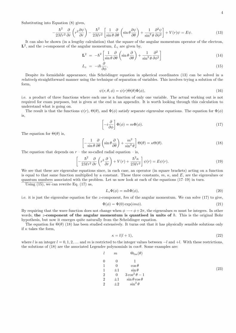
where l is an integer l = 0, 1, 2, .... and m is restricted to the integer values between −l and +l. With these restrictions,the solutions of (18) are the associated Legendre polynomials in cos θ. Some examples are:

l m Θlm(θ)

0 0 11 0 cos θ1 ±1 sin θ2 0 3 cos2 θ − 12 ±1 sin θ cos θ2 ±2 sin2 θ

(23)

5

!

0

!

0

!

0

!

0

!

0

!

0

l=0

l=1

l=2

m=0

m=±1

m=± 2m=± 1m=0

m=0

FIG. 3: Polar plots of the probability distributions |Ylm(θ, φ)|2 = |Θlm(θ)|2. Note that the probability distributions do notdepend on φ.

You can check that these are solutions by direct substitution into (18).These solutions may be multiplied by exp(imφ) and still be a solution of (18). In fact they are now solutions of

both (18) and (17) simultaneously and, apart from a constant factor, are known as the spherical harmonics. Thesecan be looked up in many books and are generally denoted, Ylm(θ, φ). They contain all the angular information aboutthe wave function of the electron. By using equations (14), (17), and (18) it can be shown that (see Problem below),

L2Ylm = h2l(l + 1)Ylm, (24)

i.e the angular momentum of the electron is given by

L = h√l(l + 1) l = 0, 1, 2, ... (25)

That leaves us with only the radial equation (19) to deal with. In order to solve this, we need an expression for thepotential V (r) and so we consider the specific case of a hydrogen atom.

PROBLEM

Prove the result shown in Eq. (24), where Ylm = Θ(θ)Φ(φ)Hint: Multiply both sides of Eq. (18) on the right by Φ(φ) and then use Eq. (17) to write the operator in the formof L2 given by (14).

6

Appendix

(N.B. This material is not examinable - it is included for your interest)

In this appendix, we show how the separation of variables technique can be used to separate the 3d Schrodingerequation in spherical coordinates into three separate eigenvalue equations. We begin by substituting Ψ(r, θ, φ) =ψ(r)Θ(θ)Φ(φ) into the Schrodinger equation. This gives,

− h2

2Mr2ΘΦ

∂

∂r

(r2∂ψ

∂r

)− h2

2Mr2

[ψΦ

1sin θ

∂

∂θ

(sin θ

∂Θ∂θ

)+ ψΘ

1sin2 θ

∂2Φ∂φ2

]+ (V (r)− E)ψΘΦ = 0 (26)

Dividing through by ψΘΦ and multiplying by 2Mr2, this can be rewritten as,[−h2 1

ψ

∂

∂r

(r2∂ψ

∂r

)+ 2Mr2(V (r)− E)

]− h2

[1Θ

1sin θ

∂

∂θ

(sin θ

∂Θ∂θ

)+

1Φ

1sin2 θ

∂2Φ∂φ2

]= 0 (27)

Using Equation (14), the second term can be rewritten to give,[−h2 1

ψ

∂

∂r

(r2∂ψ

∂r

)+ 2Mr2(V (r)− E)

]+

[1

ΘΦL2ΘΦ

]= 0. (28)

Now, the first term in square brackets depends only on r and the second term in square brackets depends only on theangular variables θ and φ. That means that these two terms must each equal a constant (and sum to zero), i.e. wecan write,

−h2 1ψ

∂

∂r

(r2∂ψ

∂r

)+ 2Mr2(V (r)− E) = −c (29)

1ΘΦ

L2ΘΦ = c, (30)

where c is a constant. The second equation is just the eigenvalue equation for L2, i.e. c = h2l(l+1), where l = 0, 1, 2, ....This means we can rewrite the radial equation as,[

− h2

2Mr2∂

∂r

(r2∂

∂r

)+ V (r) +

h2l(l + 1)2Mr2

]ψ(r) = Eψ(r). (31)

This is the same as Equation (19) above. Now, using the value for c and substituting back the derivative form of L2

into Eq. (30), we get,

− 1Θ

1sin θ

∂

∂θ

(sin θ

∂Θ∂θ

)− 1

Φ1

sin2 θ

∂2Φ∂φ2

= l(l + 1). (32)

There is no Φ(φ) dependence on the right hand side, i.e. l(l + 1), therefore, the φ-dependent term on the left handside must be a constant,

1Φ∂2Φ∂φ2

= −m2. (33)

This can be rewritten as, [−i ∂∂φ

]Φ(φ) = mΦ(φ), (34)

i.e Equation (17).Finally, substituting this into Eq. (32), and multiplying by Θ(θ), we get[

− 1sin θ

∂

∂θ

(sin θ

∂

∂θ

)+

m2

sin2 θ

]Θ(θ) = l(l + 1)Θ(θ), (35)

i.e. Equation (18).

7

IV. THE HYDROGEN ATOM

So far we have solved the 3-d Schrodinger equation for the angular coordinates, θ and φ. These coordinates areindependent of the potential V (r). In order to complete the job, and write down the full solution, we need to solvethe radial equation [

− h2

2Mr2∂

∂r

(r2∂

∂r

)+ V (r) +

h2κ

2Mr2

]ψ(r) = Eψ(r). (36)

For this we will consider the specific case of the electron in a hydrogen atoms. In this case, the electron is bound tothe proton by the Coulomb potential,

V (r) = − e2

4πε0r. (37)

This enables us to rewrite the radial equation as,[− h2

2Mr2∂

∂r

(r2∂

∂r

)− e2

4πε0r+h2l(l + 1)

2Mr2

]ψ(r) = Eψ(r), (38)

where we have written κ = l(l + 1) since we have seen that these are the only values that are consistent with thesolutions of the angular equations.

It turns out that this equation only has solutions if the energy eigenvalue takes the discrete values,

E ≡ En = − R

n2n = 1, 2, 3, ... (39)

and l < n. R is the Rydberg constant,

R =12

(e2

4πε0

)2M

h2 ≈ −13.6eV (40)

Again, we see that Bohr’s energy level spectrum has emerged as a natural consequence of the Schrodingerequation.

The solutions of Eq. (38) for ψ(r) ≡ ψnl(r) can be obtained analytically (but this is beyond the scope of thiscourse). Some examples (not normalised) are:

n l ψnl(r)

1 0 exp(− r

a0

)2 0

(1− r

2a0

)exp

(− r

2a0

)2 1 r

a0exp

(− r

2a0

) (41)

0 5 10 150

0.2

0.4

0.6

0.8

1

r/a0

!1,

0(r)

0 5 10 15!0.2

0

0.2

0.4

0.6

0.8

r/a0

!2,

0(r)

0 5 10 150

0.2

0.4

0.6

0.8

1

r/a0

!2,

1(r)

FIG. 4: Plot of the radial wave functions shown in (41).

8

where

a0 =4πε0h2

Me2≈ 5.29× 10−11m (42)

is the Bohr radius. These radial wave functions are plotted in Figure 4.To recap: The complete solution of the Schrodinger equation for a Coulomb potential has the form,

ψnlm(r, θ, φ) = ψnl(r)Θlm(θ)Φm(φ) (43)

and is labelled by three quantum numbers n, l,m. These reflect the fact that for a central potential, the originalequation could be factorised into three separate equations – one for each dimension. The complete (un-normalised)wave functions are then easily written down by using the results in (23) and (41) and the fact that Φm(φ) = exp(imφ).(Note: these tables will be given to you in an exam). For the first two energy levels (i.e. n = 1, 2) the complete wavefunctions are:

n l m ψnlm(r, θ, φ)

1 0 0 exp(− r

a0

)2 0 0

(1− r

2a0

)exp

(− r

2a0

)2 1 0 r

a0exp

(− r

2a0

)cos θ

2 1 ±1 ra0

exp(− r

2a0

)sin θ exp(±iφ).

(44)

Of course, not all values of n, l,m are possible. The energy eigenvalue En depends only on one quantum number nalso called the principal quantum number: n = 1, 2, 3, ....

The electron angular momentum states are labelled by quantum numbers l and m, where the total angular mo-mentum is h

√l(l + 1) and the component along the z-axis is mh. The values that l and m can take are,

l = 0, 1, 2, ..., n− 1m = −l,−l + 1, ..., l.

A. Another notation

There is an alternative labelling of the angular momentum states that is commonly used and which you shouldknow. This arose from the empirical classification of spectral lines into series before quantum theory was developed.In this notation, the angular momentum state l = 0 is specified by the letter s for sharp; l = 1 is specified by p forprincipal; l = 2 by d for diffuse; l = 3 by f for fundamental. After that, the letters just increase alphabetically.

l = 0 1 2 3 4 5 6 ...

s p d f g h i ...

For example, in this notation, an electron in the energy state n = 2 and angular momentum state l = 0 would besaid to be in the 2s state. For n = 4 and l = 2, it is the 4d state.

V. RADIAL PROBABILITY DENSITIES

The probability of finding an electron in a small volume dV about the point specified by the coordinates r, θ, andφ is proportional to:(a) the volume dV(b) the modulus squared of the wave function at that point, |ψ(r, θ, φ)|2.The volume element is spherical polar coordinates can be constructed from a small ‘cube’ with sides dr, rdθ, andr sin θ dφ, so that,

dV = r2 sin θ dr dθ dφ. (45)

9

Therefore, the probability of finding an electron in an energy state, n and an angular momentum state (l,m) in avolume dV at position (r, θ, φ) is,

Pnlm dV = |ψnlm(r, θ, φ)|2r2 sin θ dr dθ dφ=

[|ψnl(r)|2r2 dr

] [|Θlm(θ)|2 sin θ dθ

] [|Φm(φ)|2 dφ

],

where is the last line we have separated the variables into each of the three sets of brackets. Each of these functionsis separately normalised, so that, ∫ 2π

0

|Φm(φ)|2 dφ = 1 (46)∫ π

0

|Θlm(θ)|2 sin θ dθ = 1 (47)∫ ∞

0

|ψnl(r)|2r2 dr = 1. (48)

For example: n = 1, l = 0, m = 0

ψ1,0,0(r, θ, φ) = A exp(− r

a0

)∫ ∞

0

A2 exp(−2ra0

)r2 dr

∫ 2π

0

dφ

∫ π

0

sin θ dθ = 1

A2

(a30

4

)(4π) = 1

=⇒ A =1

√πa

3/20

where we have used the result∫∞0r2 exp(−r/b) dr = 2b3 that can be looked up in tables of integrals and would be

given to you if required in the exam.Using a similar technique, the wave functions in (44) can be normalised to give (You are not expected to memorise

these!)

n l m ψnlm(r, θ, φ)

1 0 0 1√πa

3/20

exp(− r

a0

)2 0 0 1

2√

2πa3/20

(1− r

2a0

)exp

(− r

2a0

)2 1 0 1

4√

2πa3/20

ra0

exp(− r

2a0

)cos θ

2 1 ±1 1

8√

2πa3/20

ra0

exp(− r

2a0

)sin θ exp(±iφ).

(49)

If we are only interested in the distance of the electron from the nucleus and not its direction, then the integralsover the angles can be done leaving the probability of finding an electron at a distance r.The radial probability density p(r) is given by

p(r) = |ψnl(r)|2r2. (50)

Note that the modulus squared wave function is multiplied by the geometric factor r2. For the ground state: n = 1,l = 0, E1 = −13.6eV, the wave function is,

ψnl(r) = A exp(− r

a0

). (51)

The normalisation constant is given by,

A2

∫ ∞

0

r2 exp(−2ra0

)dr = 1. (52)

10

This gives A2 = 4/a30 and so the radial probability density is,

p(r) =(

4a30

)r2 exp

(−2ra0

). (53)

This function is plotted in Figure 5(a) and peaks at the Bohr radius, r = a0. For comparison, the radial distributionfunctions for the n = 2 states are plotted in Figure 5(b-c).

0 5 10 150

0.2

0.4

0.6

r/a0

p(r)

0 5 10 150

0.4

0.8

1.2

1.6

r/a0

p(r)

0 5 10 150

0.05

0.1

0.15

0.2

n=1l=0

n=2l=0

n=2l=1

(a) (b) (c)

FIG. 5: Plot of the radial probability densities for (a) the 1s ground state, (b) the 2s state, and (c) the 2p state.

PROBLEMS

1. Show that an electron in the 2p state is most likely to be found at r = 4a0.

2. Evaluate the integral∫∞0r2 exp(−2r/a0) dr using integration by parts.

11

VI. STERN-GERLACH EXPERIMENT

In 1922, one of the most important experiments in atomic physics was carried out by Otto Stern and Walter Gerlachat the University of Frankfurt. They wanted to measure the magnetic moment of atoms that comes about from themotion of the electrons. It is well-known that, if charges move in a circle, a magnetic field is created in a directiongiven by the right-hand rule. Think, for example, of an electric current moving in a coil. In a similar way, we have seenthat charged electrons ‘orbit’ the nucleus of an atom with angular momentum L = h

√l(l + 1). This means that we

would expect the atom to have an overall magnetic field associated with it. The so-called Stern-Gerlach experimentwas designed to measure this effect.

FIG. 6: Scheme of the Stern-Gerlach experiment

The experimental apparatus (shown in Fig. 6) consisted of a furnace producing a beam of silver atoms. Thisbeam travelled through a vacuum and passed through collimators to ensure that it didn’t spread out too much. Thecollimated beam was then passed through an inhomogeneous magnetic field, which was stronger near the north polethan the south pole. Finally, the atoms were collected on a screen.

The energy of a magnetic moment, ~µ, in a magnetic field, ~B is,

E = −~µ · ~B, (54)

where the magnetic moment due to the angular momentum of the electron is,

~µ =−e~L2me

. (55)

The minus sign is because electrons are negatively charged and me is the electron mass. If we take the direction ofthe magnetic field to be the z-direction, then the energy is,

E =e

2meLzBz =

eh

2memBz, (56)

where the last equality follows from Lz = hm. The force on the atom in the magnetic field is then,

Fz = −∂E∂z

= − eh

2me

dBz

dzm. (57)

Two important points come out of this. Firstly, for a uniform field, we get dBz/dz = 0, which would mean that theforce is zero and explains why we need an inhomogeneous magnetic field. This can also be physically understood bythe fact that we need an overall net force, i.e. the upward and downward forces are not balanced. Secondly, we noticethat the force is quantized since m can only take integer values. This second fact led Stern and Gerlach to proposethat the quantization of angular momentum would result is discrete ‘blobs’ of atoms being seen on the screen. Inparticular, there should be 2l + 1 blobs since that is the number of different values m can take. This is differentfrom the classical prediction of a continuous broad distribution of atoms on the screen (since classically any angularmomentum is possible).

12

FIG. 7: Plaque at the University of Frankfurt commemorating the famous experiment.

The result were not as expected — all the most interesting experiments throw up a surprise! Although they did seediscrete blobs of atoms (rather than a continuous distribution), they only saw two blobs. The reason this is surprisingis that this would suggest 2l + 1 = 2, which means l = 1/2, but we have already seen that l must be an integer.

The explanation for all this is that the electron has an inherent magnetic moment called its spin.

A. What is this thing called spin?

Spin is a vector quantity ~S = (Sx, Sy, Sz) measured in units of h and therefore has the units of angular momentum(as we might expect for a spin). The equation for the magnitude of the spin angular momentum is,

S = h√s(s+ 1), (58)

where s is the spin quantum number and can only be an integer or half-integer.The word spin is somewhat misleading as nothing is spinning! For example, the electron is a point particle and a

point cannot spin. Despite this, it is possible to see evidence of the spin (or inherent magnetic moment) of a particlein the Stern-Gerlach experiment. In analogy with the magnetic moment due to its orbital angular momentum, theenergy of the particle in a magnetic field ~B due to its spin is

E = −g~s · ~B, (59)

where g is a constant. If we define the z axis to be in the direction of the magnetic field, we get ∆E = −gSzB. Thez-component of the spin can only take the values,

Sz = msh where ms = −s,−s+ 1,−s+ 2, ...., s (60)

and so the energy level is split into 2s+ 1 components. This means that the spin of a particle can be inferred by itsbehaviour in a magnetic field. For example, an electron is split into two components, which means that is has spin1/2. Similarly, a particle split into three energy components by a magnetic field would have spin 1.

Historical NoteWhen Gerlach first removed the detector plate from the vacuum after this experiment was carried out, nothing wasseen. There was no trace of silver. However, to his amazement, slowly the trace of the beam started to appear. AsStern later put it:

“My salary was too low to afford good cigars, so I smoked bad cigars. These had a lot of sulphur in them,so my breath on the plate turned the silver into silver sulphide, which is jet black so easily visible. It waslike developing a photographic plate.”

Had it not been for Stern’s cheap cigars, one of quantum physics greatest episodes may have passed us by.

13

VII. IDENTICAL PARTICLES AND SYMMETRY OF THE WAVE FUNCTION

So far, we have studied only the wave function for single particles. In order to study real-world problems, we wouldlike to extend this approach to consider multi-particle systems. This leads us directly to an important feature ofquantum mechanics: quantum particles of the same type are identical. Two particles are said to be identical whenthey cannot de distinguished by any intrinsic property. This means that two electrons, for example, cannot be toldapart no matter how clever we are or how hard we try. This is quite different from classical physics where objects mayappear to be the same (identical twins, two red apples....) but can always be distinguished if we look hard enough.While classical particles have sharp trajectories and so can be told apart by the paths they take, in quantum physicsthere is no way of keeping track of the individual particles when their wave functions overlap. The fact that quantumparticles are indistinguishable has some fascinating and fundamental consequences.

A. Wave function for two identical particles

As a simple example, consider two identical non-interacting particles of mass m placed in an infinite square wellwith width, L. We know that for single particles, the energy of the pth level is given by,

Ep =h2

2M

(πpL

)2

. (61)

The spatial wave function of a particle is

ψ(x) = 〈x|Ψ〉, (62)

i.e. the probability amplitude of the state |Ψ〉 having each value of position x We have seen that the wave functionfor a particle in the pth energy level is,

ψ(x) =√

2/L sin(pπx/L). (63)

Now, suppose that one particle goes into level p and the other goes into level q. Since the particles are not interacting,they should be independent of one another and, for the wave function of the two particles, we might anticipate theproduct,

ψ(x1, x2) = ψp(x1)ψq(x2) =2L

sin(pπx1

L

)sin

(qπx2

L

), (64)

where the particle in state p has been labelled by x1 and the one in q labelled x2.

0

0.5

1

00.2

0.40.6

0.81!1

!0.5

0

0.5

1

x1/Lx2/L 0

0.5

1

00.2

0.40.6

0.81!1

!0.5

0

0.5

1

x1/Lx2/L

a b

FIG. 8: Plot of (a) sin(3πx1/L) sin(πx2/L) and (b) sin(3πx2/L) sin(πx1/L)

It is interesting to ask what happens if the labels are interchanged 1 ↔ 2. In this case, the new wave functionbecomes,

ψ(x2, x1) = ψp(x2)ψq(x1) =2L

sin(pπx2

L

)sin

(qπx1

L

), (65)

14

and comparing with (64) we see that the wave function has changed, i.e ψ(x1, x2) 6= ψ(x2, x1). An example is shownin Figure 8 for p = 1 and q = 3.

More importantly, the probability distribution function has changed,

|ψ(x1, x2)|2 6= |ψ(x2, x1)|2. (66)

However, this cannot be correct since, if the particles are truly identical, then the interchange 1 ↔ 2 should not affectanything measurable (otherwise the measurement could be used to tell them apart). In particular, the wave functionψ(x1, x2) describing the two identical particles should have the property that,

|ψ(x1, x2)|2 = |ψ(x2, x1)|2. (67)

To understand this condition, let us introduce an operator P that swaps the two particles, i.e. Pψ(x1, x2) =ψ(x2, x1). Clearly, now, if we apply this operator twice, we should get the original state back (since we swap the twoparticles then swap them back again). This gives,

P2ψ(x1, x2) = ψ(x1, x2), (68)

and so P2 is just the identity and the eigenvalues of P are just ±1. In other words, we have two possibilities,

ψ(x1, x2) = ψ(x2, x1) (69)ψ(x1, x2) = −ψ(x2, x1). (70)

For the + sign, the wave function is said to be symmetric and for the − sign, it is said to be antisymmetric.So it seems that the fact that quantum particles are identical, demands that the wave function is either symmetric

or antisymmetric. We can easily construct symmetric and antisymmetric combinations for the two particles in a box.These are (respectively)

ψS(x1, x2) =1√2

[ψp(x1)ψq(x2) + ψp(x2)ψq(x1)] (71)

ψA(x1, x2) =1√2

[ψp(x1)ψq(x2)− ψp(x2)ψq(x1)] (72)

Note that the correct wave function is a linear combination of the two possibilities. The probability distributionfunctions derived from the correctly symmetrised wave function are plotted in Figure 9 and are quite different fromthose in Figure 8.

0

0.5

1

0

0.5

10

1

2

3

4

x1/L

x2/L

0

0.5

1

0

0.5

10

1

2

3

x1/L

x2/L

a b

FIG. 9: Plot of (a) |ψS(x1, x2)|2 and (b) |ψA(x1, x2)|2 for p = 1 and q = 3.

Although the two particles are non-interacting, the probability distribution function for the symmetric case favoursparticles being close together (x1 ≈ x2). Whereas the antisymmetric function keeps the particles apart since the wavefunction vanishes at x1 = x2. This is a purely quantum mechanical effect and has profound consequences for thephysical world.

15

VIII. SPIN AND THE EXCLUSION PRINCIPLE

We have seen that the wave functions of identical particles must be either symmetric or antisymmetric. Theantisymmetric form has the property that if two particles are put in the same quantum state, e.g. p = q, the wavefunction is,

ψ(x1, x2) =1√2

[ψp(x1)ψp(x2)− ψp(x2)ψp(x1)] = 0. (73)

This means that an antisymmetric wave function prevents two particles from having the same quantum numbers. Forthe symmetric wave function there is no such restriction.

• Particles described by symmetric wave functions are BOSONS – named after S.N. Bose

• Particles described by antisymmetric wave functions are FERMIONS – named after E. Fermi

All particles are either bosons or fermions – this is an innate characteristic of the particle and is closely related totheir spin. It has been shown that particles with

integer spin 0, 1, 2, .... are bosons

half-integer spin 1/2, 3/2, .... are fermions

Fermions Bosons

FIG. 10: A maximum of two spin-1/2 fermions can occupy each energy level and they must have opposite spins. There is norestriction on how many bosons can occupy a single energy level.

IX. SPIN AND STATISTICS

Systems consisting of fermions obey Fermi-Dirac statistics and systems consisting of bosons obey Bose-Einsteinstatistics. Electrons have spin +h/2 (spin up) or −h/ (spin down) and so are fermions. Consequently, no twoelectrons can have the same set of quantum numbers. This is an expression of the Pauli Exclusion Principle.

Pauli Exclusion Principle: No two identical fermions can have the same set of quantum numbers.

We can understand superconductors in terms of bosons and fermions. In a superconductor, pairs of electrons arepersuaded to form bound pairs (called Cooper pairs) which have an overall integer spin. These pairs then act asbosons and superconductivity appears when these pairs are all in the same quantum state.

Photons are bosons and so can all occupy a single quantum state – this is what laser light is. Many atoms (althoughcomposed of fermions, i.e. electrons, protons, and neutrons) have an overall integer spin and so are bosons. The 2001Nobel Prize in Physics was awarded to experimental groups who managed to produce large numbers of atoms all ina single quantum state - effectively an ‘atom laser’.

16

X. SPIN STATES AND SPIN FUNCTIONS

The two spin states of an electron, sz = +1/2 and sz = −1/2 are referred to as spin up and spin down respectively.The wave functions for these two spin states can be written as χ(↑) and χ(↓). Since the spin of a particle has nothingto do with its position in space (i.e. they are independent), the total wave function can be written as the product ofthe spatial and spin wave functions. For example, an electron (labelled 1) in the pth energy level with spin up can bewritten as

ψp(x1)χ(↑). (74)

The Pauli Exclusion Principle now allows a spin up and a spin down electron in each energy level since the extraspin quantum number enables a total antisymmetric wave function to be formed even though the spatial part issymmetric (see Figure 10).

There are two possibilities for constructing an overall wave function that is antisymmetric:

ψ(x1, x2) = (symmetric spatial part) × (antisymmetric spin part)ψ(x1, x2) = (antisymmetric spatial part) × (symmetric spin part).

We have seen that if two electrons are in the same energy state, then only the symmetric spatial part is possible(the antisymmetric part is zero everywhere) and hence must be in an antisymmetric spin state,

χ1(↑)χ2(↓)− χ1(↓)χ2(↑). (75)

This spin state has total spin S = s1 +s2 = 0 and is known as a singlet state. The total wave function of two particlesin the same energy state is then,

ψ(x1, x2) = [ψp(x1)ψp(x2)] (χ1(↑)χ2(↓)− χ1(↓)χ2(↑)) . (76)

and we see that the two spins must point in opposite directions.When the electrons are in different energy levels, more possibilities are open to the form of the wave function. The

combination (symmetric spatial part)×(antisymmetric spin part) gives,

ψ(x1, x2) = [ψp(x1)ψq(x2) + ψp(x2)ψq(x1)] (χ1(↑)χ2(↓)− χ1(↓)χ2(↑)) . (77)

The other combination (antisymmetric spatial part)×(symmetric spin part) gives three possibilities,

ψ(x1, x2) = [ψp(x1)ψq(x2)− ψp(x2)ψq(x1)]×

(χ1(↑)χ2(↑))(χ1(↑)χ2(↓) + χ1(↓)χ2(↑))(χ1(↓)χ2(↓))

(78)

The three symmetric spin states describe a total spin state of S = 1. This is known as a triplet state. The existenceof these spin states plays an important role in the fine structure of atomic spectra.

PROBLEM

A one dimensional box of width 1nm contains 11 electrons. The system is in the ground state.(a) What is the Fermi energy (i.e. energy of the most energetic fermion) assuming the electrons are non-interacting?(b) What is the minimum energy, in eV, a photon must have to excite an n = 1 electron to a higher energy state?

17

XI. PERIODIC TABLE

The state of an electron in an atom is fully specified by the four quantum numbers: n, l, m, and ms. This, combinedwith the fact that we know that electrons are fermions and so must obey the Pauli Exclusion Principle, allows us tostudy the electron configurations of atoms that are more complicated than hydrogen. In particular, it enables us tounderstand the periodic table of the elements.

The Russian chemist Dmitri Mendeleev was the first to propose, in 1867, a periodic arrangement of the elements.He did so by explicitly pointing out ‘gaps’ where undiscovered elements should exist. He could then predict theexpected properties of the missing elements. The subsequent discovery of these elements verified Mendeleev’s schemeand element number 101 has since been named in his honour.

A version of the periodic table is shown in Figure 11. The significance to physicists is the implication that there isa regularity to the structure of atoms. Quantum mechanics successfully explains this structure. We need three basicideas to see how this works:

1. The energy levels of the atom are found by solving the Schrodinger equation for multielectron atoms and dependon the quantum numbers n and l.

2. For each value of l, there are 2l+ 1 possible values for m and for each of these there are two possible values forthe spin quantum number, ms. Consequently, each value of l has 2(2l + 1) different states associated with itand each of these have the same energy. This can be summarised as,

Subshell l Number of states

s 0 2p 1 6d 2 10f 3 14

(79)

3. The ground state of the atom is the lowest-energy electron configuration that is consistent with the Pauliexclusion principle.

The energy of the electron is determined mainly by the principal quantum number n (which we have seen is relatedto the radial dependence of the wave function) and by the orbital angular-momentum quantum number, l. Generally,

FIG. 11: Periodic table of the elements.

18

the lower the value of n, the lower the energy; and, for a given value of n, the lower the value of l, the lower theenergy (though there are exceptions!). The dependence of the energy on l is due to the interaction of the electrons inthe atom with each other. In hydrogen, of course, there is only one electron, and the energy is independent of l.

The electron structure of an atom is written as a listing of all the energy levels that the electrons are in, orderedby their energy. For example, the ground state of hydrogen is 1s1 denoting one electron in the 1s state. The groundstate for helium is 1s2 and for lithium is 1s22s1. Remember that the s state can only be occupied by two electrons(because there are only two spin states) and so the third electron in lithium must go to the next lowest available level– in this case 2s. The energy ordering of the levels is as follows,

1s < 2s < 2p < 3s < 3p < 4s < 3d < 4p. (80)

Note that the order of 4s and 3d are different from what we might guess. This is the only exception to the orderingof levels that you will be expected to know.

Now we can write down the electron configurations for much more complicated atoms. For example, the groundstate configuration for arsenic (As) with atomic number 33 is,

1s22s22p63s23p64s23d104p3.

If the electron configuration for an atom is,

1s22s22p63s23p64s23d94p4,

the atom is still arsenic (33 electrons). However, this is now an excited state of arsenic since one of the 3d electronshas moved to the more energetic 4p level.

A. Ionization Energies

The ionization energy is the energy required to remove a ground-state electron from an atom and leave a positiveion behind. The ionization energy of hydrogen is 13.6eV because the ground-state energy is E0 = −13.6eV and anelectron requires a minimum of zero energy to be unbound. Figure 12 shows the ionization energy of the elements.There is a clear pattern to the values. The ionization energies for the alkali metals (e.g. Li, Na, K) on the left of theperiodic table have low values. These increase steadily across the table to reach maxima for the inert gases (e.g. He,Ne, Ar) on the right hand side of the table.

FIG. 12: Ionization energy of the elements.

19

Quantum theory can explain this structure. The inert gases have closed shells which are very stable structures andso these elements are chemically non-reactive. It takes a lot of energy to pull an electron out of a stable closed shelland so the inert gases have the largest ionization energies. The alkali metals, by contrast, have a single s-electronoutside a closed shell. This electron is easily disrupted, which is why these elements are highly reactive and have thelowest ionization energies.

PROBLEMS

1. What is the total number of quantum states of hydrogen with quantum number n = 4?

2. If the electron configuration of an atom is 1s22s22p63s23p64s2, what element is the atom?

XII. ENERGY SPECTRUM

Left to itself, an atom will be in its lowest-energy ground state. An atom can get into an excited state by absorbingenergy. This can happen, for example, by absorbing a photon or by colliding with other atoms.

One of the postulates of Bohr’s model is that an atom can jump from one stationary state of energy E0 to a higherenergy state E1 by absorbing a photon of frequency,

f =∆Eatom

h=E1 − E0

h. (81)

Because we are interested in spectra, it is more useful to write this equation in terms of wavelength,

λ =c

f=

hc

∆Eatom=

1240 eV nm∆E(in eV)

. (82)

Bohr’s idea of quantum jumps remains an integral part of our interpretation of the results of quantum mechanics.By absorbing a photon, an atom jumps from its ground state to one of its excited states. However, it turns outthat not every conceivable transition can occur. Allowed transitions between energy states, with the emission orabsorption of a photon, are governed by the following selection rules,

∆m = 0,±1∆l = ±1.

For example, an atom in an s-state (l = 0) can absorb a photon and be excited to a p-state (l = 1), but not to anothers-state or to a d-state. These rules come naturally from the conservation of angular momentum and the fact that aphoton carries one unit, h, of angular momentum. This enables us to understand the spectra of atoms.

PROBLEM

What is the longest wavelength in the absorption spectrum of hydrogen (initially in the ground state)? What is thetransition?

20

XIII. MOLECULAR BONDING

A. Ionic Bond

The simplest type of bond is the ionic bond found in salts such as sodium chloride (NaCl). Sodium has a solitary 3selectron located outside a stable electron core. This electron can be stripped away from the atom with the relativelysmall energy of 5.14eV. Chlorine by contrast is one electron short of a full shell and releases 3.62 eV when it acquiresan additional electron. Thus the formation of a Na+ ion and a Cl− ion by the donation of one electron from Na toCl requires only 5.14 eV - 3.62 eV = 1.52 eV at infinite separation.

However, the electrostatic energy of the oppositely charged ions when they are separated by a distance r is, −ke2/r2.When the separation of the ions is less than about 0.95 nm, the negative potential energy of attraction is greaterthan the 1.52 eV needed to create the ions. It therefore becomes energetically favourable for the two atoms to bondtogether to form NaCl. Since the electrostatic attraction increases as the ions get closer together, it might seem thatequilibrium is not possible and the ions will collapse into one another. This is prevented by the Pauli ExclusionPrinciple discussed in Section IX. If the ions become too close, the core electrons begin to overlap spatially. Becauseof the Exclusion Principle, this can only happen if some electrons go into higher energy quantum states. This increasein energy when the ions are pushed closer together is equivalent to a repulsion of the ions. For NaCl, the equilibrium(i.e minimum energy) separation of the ions is r = 0.236 nm. A sketch of the variation of potential energy with ionicseparation is shown in Figure 13.

FIG. 13: Variation of potential energy with separation for an ionic bond.

B. Covalent Bond

A very different mechanism is responsible for the bonding of similar or identical atoms such as gaseous hydrogen(H2), nitrogen (N2), and carbon monoxide (CO). If we calculate the energy required to create H+ and H− bytransferring an electron between two hydrogen atoms and add to this the electrostatic potential energy, we find thatthere is no distance for which the total energy is negative. In other words, two hydrogen atoms cannot form an ionicbond. Instead, the attraction is a purely quantum effect due to the sharing of the two electrons by both atoms. Thisis called a covalent bond.

We can understand covalent bonding by considering the example of two finite square wells that are close to eachother (see Figure 14). These wells represents the attractive potential the electrons experience due to the two positivelycharged nuclei. We begin by considering a single electron that is equally likely to be found in either well. Because thewells are identical, the probability density, which is proportional to |ψ|2, must be symmetric around the midpoint ofthe wells. This means that the wave function must be either symmetric or antisymmetric with respect to the wells,as shown in Figure 14.

Now, we consider the case of two electrons (i.e. one from each hydrogen atom). We know that electrons are fermions

21

(with spin 1/2) and therefore the total wave function must be antisymmetric on exchange of the electrons. The totalwave function is the product of a spatial part and a spin part. So the wave function of the two electrons can be aproduct of a symmetric spatial part and an antisymmetric spin part or of a symmetric spin part and an antisymmetricspatial part.

As can be seen in Figure 14, the probability distribution, |ψ|2 in the region between the protons is large for thesymmetric wave function and small for the antisymmetric wave function. Thus when the space part of the wavefunction is symmetric (and the electrons are in the S=0 singlet state) the electrons more likely to be found in thespace between the protons, and the protons are bound together by this negatively charged cloud. Conversely, whenthe space part of the wave function is antisymmetric (and the electrons are in the S=1 triplet state), the electronsspend very little time between the protons and do not bind them together into a molecule. The symmetric spatialwave function, therefore, has a lower potential energy. The equilibrium separation for H2 is r = 0.074 nm, and thebinding energy is 4.52 eV. For the antisymmetric spatial state, the potential energy is never negative and so there isno bonding.

!A

!S

FIG. 14: Two square wells representing protons that are close together. Between the wells, the antisymmetric spatial wavefunction of the electrons is close to zero, whereas the symmetric wave function is large.