Physica A 392 (2013) 3666–3681

Contents lists available at SciVerse ScienceDirect

Physica A

journal homepage: www.elsevier.com/locate/physa

Liquidity crisis detection: An application of log-periodicpower law structures to default predictionJan Henrik Wosnitza a,∗, Cornelia Denz b

a Institute of Business Administration, University of Muenster, Leonardo-Campus 1, 48149 Muenster, Germanyb Institute of Applied Physics, Center for Nonlinear Science, University of Muenster, Corrensstraße 2, 48149 Muenster, Germany

h i g h l i g h t s

• This study provides a quantitative description of the mechanism behind bank runs.• We diagnosed the presence of log-periodic patterns in CDS spreads.• We investigated univariate classification performances of log-periodic parameters.• These parameters appear to characterize investor behavior.• Further, they enable us to draw conclusions of banks’ refinancing options.

a r t i c l e i n f o

Article history:Received 22 July 2012Received in revised form 7 February 2013Available online 19 April 2013

Keywords:Log-periodic power lawDiscrete scale-invarianceEconophysicsBailoutDefault estimation

a b s t r a c t

We employ the log-periodic power law (LPPL) to analyze the late-2000 financial crisisfrom the perspective of critical phenomena. The main purpose of this study is to examinewhether LPPL structures in the development of credit default swap (CDS) spreads canbe used for default classification. Based on the different triggers of Bear Stearns’ nearbankruptcy during the late-2000 financial crisis and Ford’s insolvency in 2009, this studyprovides a quantitative description of the mechanism behind bank runs. We apply theJohansen–Ledoit–Sornette (JLS) positive feedback model to explain the rise of financialinstitutions’ CDS spreads during the global financial crisis 2007–2009. This investigationis based on CDS spreads of 40 major banks over the period from June 2007 to April 2009which includes a significant CDS spread increase. The qualitative data analysis indicatesthat the CDS spread variations have followed LPPL patterns during the global financialcrisis. Furthermore, the univariate classification performances of seven LPPL parametersas default indicators are measured by Mann–Whitney U tests. The present study supportsthe hypothesis that discrete scale-invariance governs the dynamics of financial marketsand suggests the application of new and fast updateable default indicators to capture thebuildup of long-range correlations between creditors.

© 2013 Elsevier B.V. All rights reserved.

1. Introduction

In economics the opinion prevails that complex financial systems are in general unpredictable [1]. Some econophysicistshave nevertheless designed methods in order to predict financial market turmoil. The interactions between microscopicparticles dealt with in physics are commonly of short range. But under certain conditions these short ranged interactionsdevelop to long ranged interactions, culminating in cooperative behavior of the physical system. Financial markets also

∗ Corresponding author. Tel.: +49 251 83 31824.E-mail addresses: j.w@uni-muenster.de (J.H. Wosnitza), denz@uni-muenster.de (C. Denz).

0378-4371/$ – see front matter© 2013 Elsevier B.V. All rights reserved.http://dx.doi.org/10.1016/j.physa.2013.04.009

J.H. Wosnitza, C. Denz / Physica A 392 (2013) 3666–3681 3667

exhibit cooperative phenomena, for instance, in terms of crashes when investors decide in bulk to sell their shares. Thisapparent similarity between physical systems on the one hand and financial market dynamics on the other hand justifiesthe application of physical methods in order to extract the coarse-grained properties of these large ensembles of marketparticipants [1–3]. In particular, the log-periodic power law (LPPL) has proven very fruitful in forecasting the bursting ofspeculative bubbles [1].

In a nutshell, the objective of the LPPL ansatz is to observe well defined patterns in price trajectories before criticalpoints in time. In this context, financial markets are regarded as self-organized systems that can drive themselves towardcritical points [4]. When financial markets approach their critical points, long-range correlations between traders build upand imitation becomes a leadingmotive of investment decision [4–6]. This positive feedbackmechanism between investorsresults in a faster-than-exponential price increase decorated by log-periodic oscillations [7]. The faster-than-exponentialprice increase is defined by a growth rate which increases with time [8]. The log-periodic oscillations manifest themselvesas peaks and valleys with progressively smaller amplitudes and greater frequencies that eventually reach the critical pointin time tc at which the average state of the system becomes sensitive to external influences [6]. Any adequate disturbancemay trigger a crash at this state. That is why the speculative bubble has the highest probability to burst at tc . For the sake ofillustration, we adopt the example originally given in Ref. [6]: ‘‘Consider a ruler put vertically on a table. Being in an unstableposition, it will fall in some direction, and the specific air current or slight imperfection in the initial condition are of no realimportance. What is important is the intrinsically unstable initial state of the ruler. We argue that a similar situation appliesfor crashes. They occur because the market has reached a state of global instability. Of course, there will always be specificevents which may be identified as triggers of market motions but they will be the indicators rather than the deep sourcesof the instability’’ [6].

In order to provide an overview of the literature on log-periodicity, we first have to mention the pioneering works ofFeigenbaum and Freund [9] and Sornette et al. [10] who independently of each other discovered ex post LPPL structures inthe S&P500 index prior to the crash in October 1987. The hypothesis that the reasons for LPPL structures are rooted deeperin economic mechanisms than only in the dynamics of financial markets has met with skepticism and even triggered aheated discussion between two discoverers [11–14]. The academic community is also divided into two camps on this topic:Although, skepticsmainly acknowledge the presence of LPPL imprints in financial time series, they consider those structuresas accidental patterns attributed to the stochastic processes of the financial market [12,15,16]. In contrast, the advocates ofthe Johansen–Ledoit–Sornette (JLS) model substantiate their point of view of LPPL patterns diagnosing speculative bubblesby offering a wide variety of investigations which can, for example, be partitioned into four groups as follows: First, there isrich literature on the ex post detection of LPPL patterns preceding financial crashes. LPPL structures were, for example,successfully identified in stock market bubbles [6,12,17–22], in real estate price bubbles [8,23], in the 2006–2008 oilbubble [24], and in the US FED Prime Rate [25].1 Second, a vast body of empirical evidence has accumulated demonstratingthat the herding behavior of investors not only results in speculative bubbles with accelerating market overvaluations, butalso in anti-bubbles with decelerating market devaluations [27–29]. A third strand of literature went even one step furtherby claiming that financial crashes can be forecasted by extrapolating the LPPL [1]. The main idea of this research line is tointegrate the LPPL structures into a pattern recognition approach in order to predict end times of bubbles and anti-bubbles[1,29–31]. Fourth, researchers have discovered that the presence of LPPL structures is predictive of crashes in real data, butthey were unable to establish a link between LPPL patterns and crashes in the synthetic data [9,32,33].

Despite this large number of studies in favor of the LPPL hypothesis, ‘‘the statistical significance of these precursors andtheir predictive power remain controversial in part’’ [34]. However, an increasing number of case studies in a wide varietyof financial time series reinforces one by one the LPPL hypothesis. The detection of LPPL structures in US corporate bondspreads [35], in the credit default swap (CDS) indices [36,37], and in the repurchase agreement market size bubble from2007 to 2008 [38] can be considered as first applications of the LPPL to credit risk time series. The experiences of the globalfinancial crisis 2007–2009 have shown plainly that high uncertainties about international banks’ creditworthiness mayinduce serious consequences for the real economy [39–42]. Due to significant off-balance-sheet liabilities, it is difficult toestimate the default risk of financial institutions on the basis of conventional methods like balance sheet ratings or withinthe Black–Scholes–Merton framework [43]. Research on the causes of international banks’ deterioration in creditworthinessis therefore of utmost importance for financial market stability. Ourmain hypothesis is that bankruptcies are not necessarilythe consequences of bad business figures, but can also be the result of creditors’ positive feedback interaction in analogy tocritical phenomena in physics. Thus, it appears to be worthwhile to pursue the idea of LPPL structures as a harbinger of animpending liquidity crisis.We consequently apply the JLSmodel to explain the CDS spreadmovements of large banks duringthe financial crisis 2007–2009 [4,44]. This model is based on two central assumptions: First, CDSs provide an opportunityfor creditors to transfer credit risks to counterparties. Hence, the individual creditor in our model has only two possibleactions: Either he does hedge or he does not hedge against default by CDSs. Second, no creditor can precisely estimate theprobability of default for any debtor. There is always an uncertainty about the obligor’s credit standing. That is why eachcreditor steadily communicates with a limited number of other creditors about the obligor’s solvency. The opinions of theirnetworks are crucial for the creditors’ future actions.

Weperformboth, a qualitative and a quantitative investigation on daily data of financial institutions’ CDS spreads in orderto answer the question whether there is a link between bankruptcies and phase transitions. At first, we calibrate the LPPL

1 Sornette [26] provides further examples of cases in which LPPL patterns were diagnosed.

3668 J.H. Wosnitza, C. Denz / Physica A 392 (2013) 3666–3681

Jan05 Jul05 Jan06 Jul06 Jan07 Jul07 Jan08 Jul08 Jan09 Jul09

BBBBBB+A−AA+

Bear Stearns

Time

S&

P’s

Rat

ing

Jan05 Jul05 Jan06 Jul06 Jan07 Jul07 Jan08 Jul08 Jan09 Jul09

SDCCCCC

B

BB

BBBFord

Time

S&

P’s

Rat

ing

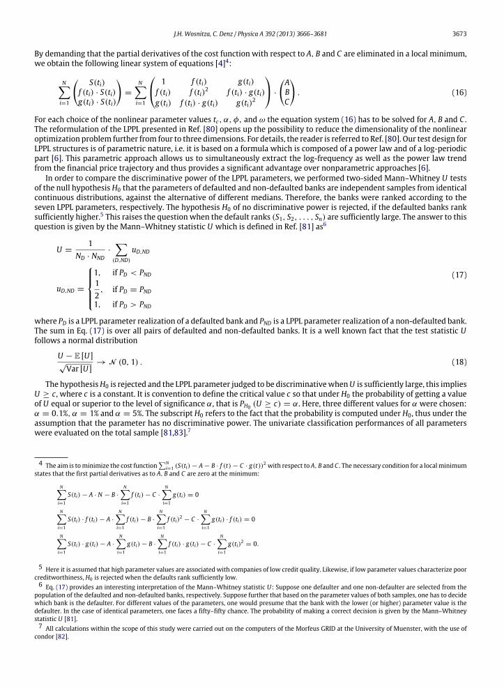
Fig. 1. Rating history of Ford and Bear Stearns. For the sake of overview, only some rating classes are displayed.

to CDS spreads of 40 financial institutions. Based on these results, we evaluate the discriminatory power of the parametervalues to separate between defaulted and non-defaulted banks using Mann–Whitney U tests. In contrast to the definitionof default specified by the Basel Committee on Banking Supervision [45], recipients of federal bailout funds are labeled asdefaults whereas financial institutions that did not require public bailouts are labeled as non-defaults in this study.

The present study contributes to the literature twofold: First, this paper provides a quantitative description of the mech-anism behind bank runs, and thus ensures better understanding of reasons for insolvencies. Second, the presence of discretescale-invariance in time series related to credit risk suggests the application of new and fast updateable default indicatorsto capture the buildup of long-range correlations between creditors.

The remainder of this paper is organized as follows: Section two briefly displays the current knowledge of the companycrises theory and shows the incompleteness of this theory. A background section about the LPPL follows in section three.Subsequently, a description of the data set and of theMann–WhitneyU test is presented in section four. The fifth section listsand briefly discusses the empirical results and finally, the sixth section summarizes the most important results, discussesthe limitations inherent to the methodology and concludes with implications for theory and practice.

2. Crisis mechanisms for companies on their way to insolvency

The business management theory assigns strategic and operative mistakes as reasons for manufacturers’ defaults [46].The course to insolvency is usually subdivided into four phases which are characterized by the isolated or combinedoccurrence of an increasing debt-to-equity ratio and liquidity shortages2:

1. Strategic crisis: The first stage of the crisis mechanism is not as clearly determinable as the stages listed below. In general,this phase is distinguished by a drop of net income, but not necessarily by an increasing debt-to-equity ratio.

2. Operative crisis: The second stage is characterized by an increasing debt-to-equity ratio and progressively noticeablelosses. As a consequence, liquid assets diminish considerably.

3. Illiquidity crisis: The company becomes heavily in debt during this penultimate stage. Since debt rises, the crisis becomesincreasingly urgent.

4. Insolvency: Finally, the company is unable tomeet its financial obligations in part or in full, because of liquidity shortages.

Ford’s road to insolvency, for instance, can be differentiated in compliance with the individual phases mentioned above:Standard and Poor’s (S&P) justified the first two consecutive downgrades of Ford’s creditworthiness illustrated in Fig. 1 on05/05/2005 and 01/05/2006 by their ‘‘skepticism about whether management’s strategies will be sufficient to counteractmounting competitive challenges’’ [48]. Further indication of the strategic crisis is provided by S&P opinion that ‘‘thefull-year pretax loss of Ford’s North American operations could approach $2 billion – before substantial impairment andrestructuring charges – although Ford is still expected to be profitable on a net basis in 2005 (before special items) thanksto earnings from its finance unit’’ [49]. According to S&P, an operative crisis characterized by ‘‘mounting cash losses inFord’s North American automotive operations’’ [50] has unfolded on 07/31/2008. Strictly speaking, S&P decision to lowerthe rating on FordMotor Company on 07/31/2008was driven by ‘‘cash outflows (which)will reduce the company’s currentlyadequate liquidity’’ [50]. Ford’s transition to illiquidity crisiswas documented by S&P expectation that ‘‘Ford’s liquidity (will)be significantly reduced the rest of this year and into next year by continued heavy cash use’’ [51]. Ford’s announcement of adebt restructuring on 03/04/2009 induced S&P to demote the company’s rating from CCC+ to CC [52]. Given that distressed

2 The theoretical considerations on Section 2 are based on [47].

J.H. Wosnitza, C. Denz / Physica A 392 (2013) 3666–3681 3669

exchanges belong to S&P default criteria, Ford’s rating was lowered to SD (selective default) after completion of the tenderoffers on 04/06/2009 [53].

Assuming a four stage process in the run-up to insolvency justifies the hope that balance sheet ratios are capable of dis-criminating between defaulted and non-defaulted companies with a forecast horizon greater than one year. But the suddendecline of creditworthiness of several banks during the financial crisis 2007–2009 arises doubt on the validity of the just pre-sented concept for financial institutions. In contrast to manufacturing firms, financial institutions are subject to bank runs,i.e., to the risk of becoming illiquid due to loss of investors’ confidence. Balance sheet ratios usually cannot reflect this risk.Motivated by Bear Stearns’ collapse shown in Fig. 1, we posit that illiquidity crisis can also be triggered or at least intensifiedby the nonlinear interaction of creditors [54]. S&P raised Bear Stearns’ credit rating from A to A+ on 10/27/2006 based onthe company’s ‘‘relatively low profit volatility, conservativemanagement, and cost flexibility, as well as long-term improve-ments in its liquidity and risk management’’ [55]. This upgrade was compensated by a later rating action on 11/15/2007reflecting Bear Stearns’ first quarterly loss in its history due to a ‘‘writedown on its CDO and subprime exposure’’ [56]. Fi-nally, Bear Stearns spiraled into an existence-threatening crisis on 03/14/2008 since ‘‘its liquidity position has substantiallydeteriorated in the past 48 hours [54]. The company’s announcementwas followed by S&P downgrade on Bear Stearns’ fromA to BBB. The minor rating judgment deterioration on Bear Stearns is explained by S&P expectation ‘‘that Bear will find anorderly solution to its funding problems’’ [54]. Over the weekend of 03/15/2008, the US Federal Reserve, the US Depart-ment of the Treasury and JPMorgan Chase prepared a rescue takeover to prevent Bear Stearns from going bankrupt [57–59].JPMorgan completed the acquisition of Bear Stearns on 05/30/2008 [59].

In contrast to Ford Motor Company, whose liquidity crunch was attributed to its North American automotive opera-tions [49–51,60], Bear Stearns’ near-bankruptcy in March 2008 was at least partially a different story: This collapse wasmainly caused by a run of the counterparties on the investment bank [57,61]. In concrete terms, lenders denied credits andclients withdrew their liquid assets from Bear Stearns due to a lack of trust [61,62].

Skipping or speeding through the strategic or operative crisis, as with Bear Stearns, may shorten the forecasting horizonof default prediction. As a result, balance sheet ratiosmay be inadequate indicators of defaults triggered by a run of creditorsand customers, since they can only be updated annually for the greater part [63]. In the next section we apply the JLS modelintroduced by Johansen et al. [4] to explain how the nonlinear interaction of creditors may have caused Bear Stearns’ failure.Following this model, new default predictors are suggested.

3. Model to explain LPPL patterns in CDS spreads

Johansen et al. [4] proposed amodification of the Ising spin model, in which investors either imitate the opinions of theirnearest neighbors or take individual decisions, in order to formalize the information swap between investors which mayeventually end up in a cooperative herding behavior of the investors [2,4,12]. According to this model, speculative bubblesemerge from a positive feedback mechanism. As a new area of application, it is demonstrated that this model can be usedto explain the CDS spread variations of several banks during the financial crisis 2007–2009.

CDSs enable institutional investors to transfer the credit risk of a reference entity (e.g. bank, corporate or sovereign)from one party to anotherwithout exchange of liquidity on transaction date. These financial derivatives serve the purpose ofhedging against risks of real business transactions. The design of a standard CDS contract corresponds to that of an insurance:The protection buyer purchases protection against the risk of a credit event by the underlying company from the protectionseller. A credit event refers to a legally defined event which usually incorporates bankruptcy, failure-to-pay and sometimesdebt restructuring events. To pay for the protection, the buyer of the CDS makes periodic premium payments to the sellereither until the specified maturity date of the contract or until a credit event occurs, whichever is earlier. The quoted CDSspread at conclusion of the contract determines the level of the periodic payments. The premium level is paid on the nominalvalue of the protection. In return, the protection buyer of the CDS gains the right to sell a particular bond issued by thereference entity at par value or to receive the difference between the par value and the market price if a credit event occursbefore maturity [64,65].

Roughly summarized, CDS spreads reflect investors’ aggregate opinion about the credit quality of the reference entity.Below, S(t) denotes the CDS spread at time t . For the sake of simplicity, we consider CDSs in the following as purelyspeculative investments. Furthermore we posit that themartingale hypothesis applies for the expectation of the CDS spreadS(t)—a hypothesis which holds true only under idealized conditions [4]:

E[S(t)] = S(t0) ∀t > t0. (1)

The point of departure for the model of Johansen et al. [4] is the following Ising spin model [4]3:

si = sign

j∈N(i)

sj + σ · εi + G

. (2)

A spin-up constituent represents an individual investor i who takes on credit risk (si = +1) and a spin down constituentrepresents a traderwho has already transferred the default risk to a trading partner via a CDS (si = −1) [4]. The derivation of

3 The spins si must not be confused with the CDS spread S(t).

3670 J.H. Wosnitza, C. Denz / Physica A 392 (2013) 3666–3681

the analytical solution (13) necessitates the following two main simplifications: First, each creditor pursues an irreversibleinvestment strategy which means that all investors who have already hedged against default, cannot reassume the creditrisk [66]. Second, the model presupposes that the number of insurance providers remains constant during the time whencreditors’ highly nonlinear behavior evolves. An assumption which obviously stands in opposition to the equilibriumbetween protection buyers and protection sellers [66]. Eq. (2) says, that the investment decision of a single creditori ∈ 1, . . . , I is dependent on his network’s accumulated actions, on an idiosyncratic signal εi and on a global influenceG. N(i) denotes the number of investors who significantly influence the opinion of creditor i. The scalar multipliers K and σdetermine the individual creditors’ tendency to imitate and to contradict their nearest neighbors’ opinions, respectively [4].

After defining the cumulative distribution function of the time to insolvency Q (t) and the corresponding probabilitydensity function q(t) =

∂∂tQ (t), we are able to express the hazard rate h(t) [4]:

h(t) =q(t)

1 − Q (t). (3)

At the critical point of time t = tc two scenarios are conceivable with regard to the fate of the debtor: On the one hand theinteraction of the creditors could in fact force the debtor into bankruptcy. In consequence, the creditors who hedged againstdefault would receive the agreed payoff and the CDS is taken off the market. On the other hand the debtor could survive thespeculative attack [4]. In this case we assume that the CDS spread drops by a fixed percentage κ above the inner credit riskmeasured by Sinternal. Formally, the spread trend is described by the following differential equation [33]:

dS = µ(t) · S(t) · dt − κ · [S(tc) − Sinternal] · dj, (4)

where µ(t) denotes the time-dependent drift. Applying the expectation value on both sides of Eq. (4), the martingalehypothesis (1) and the relationship E[dj] = h(t) · dt yields [4]:

µ · S(t) = κ · [S(tc) − Sinternal] · h(t). (5)

Eq. (6) is obtained by inserting (5) in (4):

dS = κ · [S(tc) − Sinternal] · h(t) · dt − κ · [S(tc) − Sinternal] · dj. (6)

As long as no default has occurred, the variable j equals zeros. Thus, Eq. (6) simplifies to:

dS = κ · [S(tc) − Sinternal] · h(t) · dt. (7)

Under the assumption that Sinternal depends only weakly on time, the integration of Eq. (7) approximately yields [33]:

S(t) ≈ S(t0) + κ · [S(tc) − Sinternal] ·

t

t0h(t ′) · dt ′. (8)

With Eq. (8) it is easy to see that the time dependence of CDS spreads before tc is only due to the hazard rate h(t). Inour simplified model the susceptibility of the system is defined by the derivation of the expected average state E[M] =

1I · E

I

i=1 siwith respect to the global influence G [4]:

χ =∂

∂GE[M]

G=0

. (9)

The susceptibility provides a measure for the system’s response to an infinitesimal global perturbation dG [4]. In physicalsystems governed by discrete scale invariance, the susceptibility close to second order phase transitions is approximately afunction of the form [4]:

χ(Kc − K) = (Kc − K)−β·

a + b · cos

ω · ln(Kc − K) + φ

, (10)

where a and b are positive constants, β > 0 denotes the critical exponent of the susceptibility and Kc stands for thecritical value for the coupling strength K : If the coupling strength K is considerably less than Kc , the creditors respondinconsistently to small global perturbations and as a result, there is little effect on the average state of the system. But if thecoupling strength K converges toward Kc , the creditors respond identically to small global influences. As a consequence ofthe investors’ homogeneous responsiveness, the system’s sensitivity to small global influences becomes extremely high [4].Since the temporal dependence of the coupling strength K is unknown, we only assume that a first order Taylor expansionaround the critical point is possible [4]:

K(t) ≈ Kc + C · (tc − t), (11)

where C is another constant. The difference tc − t quantifies the distance between the current state of the system and thecritical point. Based on Johansen et al. [4], we assume that the hazard rate follows a similar process as the susceptibility:

h(tc − t) = (tc − t)−β·

A + B · cos

ω · ln(tc − t) + φ

, (12)

J.H. Wosnitza, C. Denz / Physica A 392 (2013) 3666–3681 3671

with new constants A and B. The sensitivity of the financial market to external influences increases while approaching thecritical point in time [6]. If β would not lie within the interval (0; 1), the CDS spread would diverge under the condition thatno default has occurred yet [4,33]. Substituting Eq. (12) into (8) finally yields the LPPL for the CDS spread development [33]:

S(t) = A + B · (tc − t)α + C · (tc − t)α · cos (ω · ln(tc − t) + φ) . (13)

The existence of positive feedbacks among creditors leads to a faster-than-exponential CDS spread increase in the formof a finite-time singularity occurring at the critical time tc . However, this mathematical singularity does not exist in realdata, inter alia, because of finite-size effects [67]. Particular importance has been attached to the third summand in theLPPL (13) due to which the faster-than-exponential CDS spread growth is decorated by log-periodic oscillations. As aconsequence of these oscillations, LPPL fits can ‘‘lock in’’ on the log-periodic fluctuations and eventually lead tomore accurateestimations of the critical times tc [5]. Within the scope of this article, the faster-than-exponential growth decorated by log-periodic oscillations is referred to as LPPL structures. In addition, it should be noted that the LPPL (13) is only a first orderapproximation [5]. The log-periodic component in the noisy financial data does of course not correspond to a pure cosineas implied by Eq. (13). Nonetheless, the LPPL (13) has proven successful in capturing the mechanisms of positive feedbacksamong investors and thus in modeling the speculative aspects of financial markets [68].

The parameters in Eq. (13) have the following meaning: A represents the CDS spread S (t) in the limit t → tc [1]. Bgoverns the polynomial trend over the course of time [18,69] and C quantifies the amplitude of the log-periodic oscillationsaround this trend [1]. The critical point in time tc is themost probablemoment at which the financial market is transitioningfrom the speculative bubble into another state, for example, into a crash [4,5,67]. The end of the speculative bubble at tc doesnot necessarily imply a crash, but it is the time when a crash is most likely. Apart from the crash scenario at tc , the bubblemay either burst prior to tc or even land smoothly without any crash [6]. According to prior investigations, bubbles landsmoothly in approximately in one third of the cases [30,70]. The critical exponent α quantifies the acceleration of the CDSspreads [8] and thus is promising in capturing the collective organization between investors [71]. α is bounded between 0and 1 because otherwise the price at tc would tend toward an infinite value. Substituting φ = −ω · ln (τ ) in the cosinusterm in Eq. (13) yields [10]:

S(t) = A + B · (tc − t)α + C · (tc − t)α · cos

ω · lntc − t

τ

. (14)

According to Eq. (14), the parameter φ is regarded as time scale [10]. The log-angular frequency ω contains informationon how fast the oscillations contract. Sornette et al. [10] suggested that the term exp

πω

measures the ‘‘coupling between

traders and the fundamentals of the economy’’ [10].The JLSmodel does not explicitly impose any restrictions on the amplitude of the crash. However, depending onwhether

the crash amplitude is assumed to be proportional to the spread or to the accretion during the bubble episode, either thespread itself or the logarithm of the spread becomes implicitly the relevant observable [8,19,28]. In the remainder of thispaper, we assume that the spread itself is the natural variable.

By way of illustration, we demonstrate the key principles of the model in the following example which is depicted inFig. 2 [66,72]. At the beginning (t = 1) four creditors grant loans to one debtor. Each creditor is assigned a stress value σ0.This value determines the likelihood that creditor i transfers his default risk to a counterparty in the next instant. Creditori = 2 is the first who hedges against the potential default of the borrower at t = 2. At first only creditor i = 1 has theprivilege to use this information for his own investment decision and since he is aware that his ratings may be, at least insome cases, incorrect this information is an important factor for his own decision. The additional information is reflectedby the higher stress value. The creditors i = 3 and i = 4 do not significantly interact with creditor i = 1 and therefore thisadditional information is withheld from them. Only after creditor i = 1 has hedged his exposure, creditors i = 3 and i = 4receive the information on the two risk-hedgings which leads to an increase of both stress values at t = 3. Next creditori = 4 insures himself against potential losses via a CDS at t = 4. Since more and more creditors hedge against a possibleinsolvency and the number of CDS providers remains constant with respect to time, the CDS spread increases. This leads tohigher credit risk in the sense of a self-fulfilling prophecy, because some investors convert CDS spreads into implicit defaultprobabilities to estimate the debtor’s creditworthiness [65,73].

4. Used data and applied method

In the present analysis, CDS spreads played a similar role as the concentration of chlorine ions in the examination ofthe Kobe earthquake [74] or stock market indices in other scientific papers [3,17,75]. More specifically, we analyzed thespread trajectories of senior CDSs with 1-year maturities. Such spreads are daily monitored and available for downloadingat Thomson Reuters [76]. The data sample contained daily CDS spreads of 40 international banks from June 2007 untilapproximately April 2009, which corresponds to about 460 data points per time series. Thereof 20 financial institutionsreceived federal bailouts during the financial crisis 2007–2009. Deviating from the default definitions of the Basel Committeeon Banking Supervision [45], banks were labeled as defaults, if they have required public bailouts in the period from 2007to 2009.

In a first step, the seven parameters in the LPPL (13)were adjusted to each of the 40 CDS spread trajectories byminimizingthe squared residuals between the data points and the LPPL function. The first data point of each fitting interval corresponds

3672 J.H. Wosnitza, C. Denz / Physica A 392 (2013) 3666–3681

(t=1)

σ0

σ0

σ0

σ0

invested stressed hedged

(t=2)

σ0

σ0

σ0

σ0CDS2⋅σ

0

(t=3)

σ0

σ0

σ0

σ0CDS2⋅σ

0CDS 2⋅σ0

2⋅σ0

(t=4)

σ0

σ0

σ0

σ0CDS2⋅σ

0CDS 2⋅σ0

2⋅σ0CDS4⋅σ

04⋅σ

0

Fig. 2. Illustrative example of stress transfer. At first, each creditor is assigned an individual stress value σ0 . A higher stress value usually indicates higherrisk aversion which causes an immediate effect on the investors’ subsequent action. Creditor i = 2 is the first who decides to hedge against a potentialdefault (t = 2). His stress is transferred to creditor i = 1. Next, Creditor i = 1 insures against default transferring stress to traders i = 3 and i = 4 at t = 3.Then, creditor i = 4 buys protection at t = 4.Source: Based on [66,72].

to the lowest CDS spread prior to the commencement of the bubble. This procedure discounts the possibility that inceptionsof speculative bubbles could be clouded in uncertainty. Instead, we assumed that the interval start points can always bedetermined objectively. The last data point is equivalent to the highest CDS spread, respectively. Since we use the highestCDS spread as a last data point, our approach runs the risk of biasing the predictive power of the critical point in time tc .Under the assumption that the critical points in time are close to the last data points and that defaulted banks tend to exhibitthe maximum CDS spread earlier than non-defaulted banks, we would artificially introduce discriminative power to tc byour approach. In order to assess this risk, we conducted a Mann–Whitney U test of the predetermined fitting interval endtimes. The result indicates that there is no significant difference between the last data points of defaulted and non-defaultedbanks at a 5% level. More specifically, the AUROC value of 0.67125 indicates a sub-acceptable discriminative power of thelast data points according to Ref. [77]. Thus, we rejected the potential criticism that the discriminative power of the criticaltime tc was contaminated by a forward-looking bias.

After specifying the fitting intervals, the LPPL parameters were adjusted to the corresponding CDS spread developments.In order to achieve the best possible fit of Eq. (13) to each trajectory, we applied a multi-start optimization algorithm [78]based on the MATLAB function fmincon.m [79]. This local search algorithm ‘‘attempts to find a constrained minimum ofa scalar function of several variables starting at an initial estimate’’ [79]. In order to ensure that the outputted parametervector corresponds to a global and not only to a local minimum sum of squared residuals, we called fmincon.m 250 timeswith randomly chosen initial parameter vectors bounded as follows:

• A > 0,• B < 0 [1,18],

• −B ≥

1 +

ωα

2· |C | [1,33],

• α ∈ (0; 1) [3,4],• φ ∈ [0; 2π ] and• ω ∈ [0; 20].

We kept the five best outcomes of this search algorithm for each CDS spread trajectory. The constraint−B ≥

1 +

ωα

2·

|C | results from the fact that the hazard rate – as a probability – remains always positive [33]. Furthermore, we only considerparameter sets whose log-frequency ω is smaller than 20, ‘‘because a large log-frequency corresponds to many oscillationswhichmost often can be associatedwith high frequency noise’’ [6]. These constraints limit the parameter space to be scannedand hence may significantly reduce the computational cost. By slaving the three linear parameters A, B and C to the fournonlinear parameters tc, α, φ, andω, the LPPL fits become effectively four dimensional [4]. After substituting f (t) = (tc−t)αand g(t) = (tc − t)α · cos (ω · ln(tc − t) + φ) in Eq. (13) we can rewrite this equation as [4]:

S(t) = A + B · f (t) + C · g(t) (15)

J.H. Wosnitza, C. Denz / Physica A 392 (2013) 3666–3681 3673

By demanding that the partial derivatives of the cost function with respect to A, B and C are eliminated in a local minimum,we obtain the following linear system of equations [4]4:

Ni=1

S(ti)f (ti) · S(ti)g(ti) · S(ti)

=

Ni=1

1 f (ti) g(ti)f (ti) f (ti)2 f (ti) · g(ti)g(ti) f (ti) · g(ti) g(ti)2

·

ABC

. (16)

For each choice of the nonlinear parameter values tc, α, φ, and ω the equation system (16) has to be solved for A, B and C .The reformulation of the LPPL presented in Ref. [80] opens up the possibility to reduce the dimensionality of the nonlinearoptimization problem further from four to three dimensions. For details, the reader is referred to Ref. [80]. Our test design forLPPL structures is of parametric nature, i.e. it is based on a formula which is composed of a power law and of a log-periodicpart [6]. This parametric approach allows us to simultaneously extract the log-frequency as well as the power law trendfrom the financial price trajectory and thus provides a significant advantage over nonparametric approaches [6].

In order to compare the discriminative power of the LPPL parameters, we performed two-sided Mann–Whitney U testsof the null hypothesis H0 that the parameters of defaulted and non-defaulted banks are independent samples from identicalcontinuous distributions, against the alternative of different medians. Therefore, the banks were ranked according to theseven LPPL parameters, respectively. The hypothesis H0 of no discriminative power is rejected, if the defaulted banks ranksufficiently higher.5 This raises the question when the default ranks (S1, S2, . . . , Sn) are sufficiently large. The answer to thisquestion is given by the Mann–Whitney statistic U which is defined in Ref. [81] as6

U =1

ND · NND·

(D,ND)

uD,ND

uD,ND =

1, if PD < PND12, if PD = PND

1, if PD > PND

(17)

where PD is a LPPL parameter realization of a defaulted bank and PND is a LPPL parameter realization of a non-defaulted bank.The sum in Eq. (17) is over all pairs of defaulted and non-defaulted banks. It is a well known fact that the test statistic Ufollows a normal distribution

U − E [U]√Var [U]

→ N (0, 1) . (18)

The hypothesisH0 is rejected and the LPPL parameter judged to be discriminativewhenU is sufficiently large, this impliesU ≥ c , where c is a constant. It is convention to define the critical value c so that under H0 the probability of getting a valueof U equal or superior to the level of significance α, that is PH0 (U ≥ c) = α. Here, three different values for α were chosen:α = 0.1%, α = 1% and α = 5%. The subscript H0 refers to the fact that the probability is computed under H0, thus under theassumption that the parameter has no discriminative power. The univariate classification performances of all parameterswere evaluated on the total sample [81,83].7

4 The aim is tominimize the cost functionN

i=1 (S(ti) − A − B · f (t) − C · g(t))2 with respect to A, B and C . The necessary condition for a localminimumstates that the first partial derivatives as to A, B and C are zero at the minimum:

Ni=1

S(ti) − A · N − B ·

Ni=1

f (ti) − C ·

Ni=1

g(ti) = 0

Ni=1

S(ti) · f (ti) − A ·

Ni=1

f (ti) − B ·

Ni=1

f (ti)2 − C ·

Ni=1

g(ti) · f (ti) = 0

Ni=1

S(ti) · g(ti) − A ·

Ni=1

g(ti) − B ·

Ni=1

f (ti) · g(ti) − C ·

Ni=1

g(ti)2 = 0.

5 Here it is assumed that high parameter values are associated with companies of low credit quality. Likewise, if low parameter values characterize poorcreditworthiness, H0 is rejected when the defaults rank sufficiently low.6 Eq. (17) provides an interesting interpretation of the Mann–Whitney statistic U: Suppose one defaulter and one non-defaulter are selected from the

population of the defaulted and non-defaulted banks, respectively. Suppose further that based on the parameter values of both samples, one has to decidewhich bank is the defaulter. For different values of the parameters, one would presume that the bank with the lower (or higher) parameter value is thedefaulter. In the case of identical parameters, one faces a fifty–fifty chance. The probability of making a correct decision is given by the Mann–Whitneystatistic U [81].7 All calculations within the scope of this study were carried out on the computers of the Morfeus GRID at the University of Muenster, with the use of

condor [82].

3674 J.H. Wosnitza, C. Denz / Physica A 392 (2013) 3666–3681

Table 1List of non-bailout banks. LPPL parameters for financial institutions which did not require public bailouts in the period from 2007 to 2009.Source: Author’s calculation.

Names of banks A B C tc α φ ω

Australia & NZ BKG GP 2.57 · 10+2−6.35 · 10+1

−2.42 · 10+0 03/10/2009 2.11 · 10−1 2.18 5.54Banco Bilbao Vizcaya ARG 3.58 · 10+5

−3.56 · 10+5−8.83 · 10+1 08/03/2009 5.87 · 10−4 6.25 2.37

Banco STDR CTL HISP SA 2.34 · 10+5−2.33 · 10+5

−1.98 · 10+1 01/22/2010 5.64 · 10−4 3.12 6.63Barclays bank PLC 6.32 · 10+2

−2.20 · 10+2+9.26 · 10+0 04/12/2009 1.65 · 10−1 0.75 3.93

Commonwealth bank of AUS 1.41 · 10+2−8.36 · 10+0

+4.51 · 10−1 03/10/2009 4.33 · 10−1 2.81 8.02Credit Suisse Group 8.42 · 10+2

−4.22 · 10+2−1.23 · 10+1 03/26/2009 1.09 · 10−1 5.05 3.74

Daiwa Securities GP INC 8.82 · 10+2−2.37 · 10+2

+1.86 · 10+1 03/11/2009 2.15 · 10−1 0.84 2.73Deutsche bank AG 1.84 · 10+2

−1.20 · 10+1−1.45 · 10+0 03/13/2009 4.30 · 10−1 0.23 3.52

HSBC bank PLC 2.20 · 10+2−2.70 · 10+1

−2.66 · 10+0 03/15/2009 3.34 · 10−1 0.85 3.36Intesa Sanpaolo SPA 1.99 · 10+5

−1.98 · 10+5+2.87 · 10+1 08/24/2009 5.62 · 10−4 6.02 3.88

Mediobanca SPA 6.95 · 10+2−3.66 · 10+2

−1.07 · 10+1 04/11/2009 1.02 · 10−1 5.95 3.52Mitsubishi UFJ FIN GRP INC 9.46 · 10+1

−1.68 · 10+1−1.46 · 10+0 11/21/2008 2.63 · 10−1 0.00 2.99

National Australia bank 2.57 · 10+7−2.57 · 10+7

+6.67 · 10+0 05/30/2009 2.38 · 10−6 4.55 7.49Nordea bank AB 1.70 · 10+7

−1.70 · 10+7−7.88 · 10+0 04/06/2009 3.14 · 10−6 2.39 4.17

Rabobank 1.37 · 10+5−1.37 · 10+5

−2.01 · 10+1 04/11/2009 5.72 · 10−4 4.01 3.88Skens Banken AB 3.53 · 10+3

−3.02 · 10+3−1.46 · 10+1 04/12/2009 2.44 · 10−2 0.36 4.56

Standard CHT bank 3.64 · 10+2−2.21 · 10+1

−6.37 · 10+0 04/01/2009 4.74 · 10−1 5.75 1.46Svenska HANDBKN 3.84 · 10+2

−1.82 · 10+2−7.33 · 10+0 03/19/2009 1.14 · 10−1 4.05 2.51

Unicredito Italiano SPA 4.40 · 10+5−4.40 · 10+5

−1.57 · 10+1 03/10/2009 1.21 · 10−4 1.08 3.40Westpac banking CORP 1.03 · 10+2

−3.92 · 10+0−2.46 · 10−1 03/10/2009 4.96 · 10−1 6.28 7.91

Table 2List of bailout banks. LPPL parameters for financial institutions which did require public bailouts in the period from 2007 to 2009.Source: Author’s calculation.

Names of banks A B C tc α φ ω

Allied Irish Banks 2.84 · 10+7−2.84 · 10+7

−8.51 · 10+1 03/10/2009 4.91 · 10−6 5.65 1.64Bank of America CORP 2.71 · 10+7

−2.71 · 10+7−6.11 · 10+1 04/04/2009 5.09 · 10−6 2.98 2.03

Bank of Ireland 1.80 · 10+3−9.61 · 10+2

−3.60 · 10+1 03/08/2009 1.04 · 10−1 6.28 1.45Bear Stearns COS 1.48 · 10+8

−1.48 · 10+8−1.33 · 10+2 03/14/2008 1.45 · 10−6 3.17 1.25

Bradford & Bingley PLC 2.80 · 10+3−7.39 · 10+2

+1.22 · 10+2 10/08/2008 2.45 · 10−1 4.69 1.26Citigroup INC 4.73 · 10+5

−4.72 · 10+5−3.18 · 10+1 03/11/2009 3.30 · 10−4 4.53 4.89

Erste group bank AG 4.13 · 10+7−4.13 · 10+7

+1.86 · 10+1 03/10/2009 2.35 · 10−6 0.36 4.07Fortis NL 8.15 · 10+7

−8.15 · 10+7−1.16 · 10+2 12/07/2008 2.03 · 10−6 0.90 1.27

IKB DT INDUSTR bank AG 3.30 · 10+5−3.05 · 10+5

+5.65 · 10+3 04/20/2008 1.58 · 10−2 0.36 0.85JPMorgan chase & CO 2.80 · 10+2

−7.38 · 10+1+2.85 · 10+0 03/10/2009 1.96 · 10−1 1.53 5.08

KBC group NV 5.62 · 10+2−1.22 · 10+2

−1.12 · 10+1 03/14/2009 2.44 · 10−1 4.84 2.64Landsbanki ISLE HF 5.45 · 10+3

−3.61 · 10+3+1.25 · 10+2 10/02/2008 6.65 · 10−2 4.57 1.62

Lloyds TSB bank PLC 1.46 · 10+7−1.46 · 10+7

−9.26 · 10+0 03/14/2009 3.47 · 10−6 1.96 4.46RAIF ZNTRLBK OSTER AG 6.07 · 10+5

−6.06 · 10+5−3.44 · 10+1 03/07/2009 1.73 · 10−4 2.45 3.05

Sberbank 1.92 · 10+4−1.26 · 10+4

−3.21 · 10+3 10/29/2008 9.55 · 10−2 6.28 0.36Swedbank AB 1.41 · 10+6

−1.41 · 10+6+2.37 · 10+1 03/19/2009 5.80 · 10−5 2.71 3.45

UBS AG 8.94 · 10+5−8.93 · 10+5

+1.52 · 10+1 03/15/2009 9.60 · 10−5 4.30 5.64VTB Bank 2.73 · 10+3

−6.28 · 10+2−1.86 · 10+2 10/27/2008 2.89 · 10−1 3.33 0.94

Washington MUT INC 1.58 · 10+9−1.58 · 10+9

−7.58 · 10+2 09/24/2008 9.21 · 10−7 5.93 1.60Wells Fargo & CO 2.41 · 10+7

−2.41 · 10+7−3.49 · 10+1 04/04/2009 3.84 · 10−6 2.51 2.15

5. Application of the model to the financial crisis 2007–2009

LPPL structures are evident for all 40 banks during the time period from June 2007 until around April 2009. The optimalparameter combinations for each of the 40 banks are shown in Table 1 and in Table 2.

Instead of verbalizing these two tables in detail, we focus on summarizing typical parameter ranges for default andnon-default banks, respectively. In doing so, we have constructed box-plots of the non-linear parameters tc, α, φ, and ωin Figs. 3–6. These box-plots allow comparisons between the univariate distributions of the default banks and of the non-default banks. On each box, the central (red) mark represents the median and the box’s edges correspond to the 25th and75th percentiles, respectively. Every point outside of the 25th and the 75th percentile is regarded as an outlier. Outliers areplotted individually and are denoted by (red) plus signs (+). Typical parameter ranges for default and non-default banksare, for example, bounded by the 25th and the 75th percentiles.

Next, we investigate whether ourω-values confirm the hypothesis of an universal log-angular frequency close to nine aswas postulated, for example, in Refs. [13,84,85]. As can be seen fromFig. 6, our results indicate that the log-angular frequencywithin the analyzed CDS spread trajectories tend to be smaller than the proposed value of ω ≈ 9. The overall median ωamounts to 3.3824. The median ω of the non-default population is equal to 3.8097 and within the default population it is

J.H. Wosnitza, C. Denz / Physica A 392 (2013) 3666–3681 3675

Mar08 Sep08 Mar09 Sep09 Mar10

Non−Defaults

Defaults

tc

Fig. 3. Box-plot of the LPPL parameter tc . The central (red)marks denote themedian tc ’s within the populations of the default banks (03/09/2009) and of thenon-default banks (03/29/2009), respectively. The box’s edges represent the 25th and 75th percentiles, respectively. Every point outside of the 25th andthe 75th percentile is regarded as an outlier. Outliers are plotted individually and are denoted by (red) plus signs (+). Typical parameter ranges for defaultand non-default banks are defined by the 25th and the 75th percentiles, i.e. [10/18/2008; 03/14/2009] for default banks and [03/11/2009; 04/12/2009]for non-default banks. (For interpretation of the references to colour in this figure legend, the reader is referred to the web version of this article.)

0 0.1 0.2 0.3 0.4 0.5

Non−Defaults

Defaults

α

Fig. 4. Box-plot of the LPPL parameter α. The central (red) marks denote the median α’s within the populations of the default banks (1.3471 · 10−4) andof the non-default banks (0.1116), respectively. The box’s edges represent the 25th and 75th percentiles, respectively. Every point outside of the 25thand the 75th percentile is regarded as an outlier. Outliers are plotted individually and are denoted by (red) plus signs (+). Typical parameter ranges fordefault and non-default banks are defined by the 25th and the 75th percentiles, i.e. [3.6527 · 10−6

; 0.0996] for default banks and [5.6766 · 10−4; 0.2986]

for non-default banks. (For interpretation of the references to colour in this figure legend, the reader is referred to the web version of this article.)

1.8325. However, we acknowledge that the universal log-angular frequency of ω ≈ 9 was substantiated by numerousanalyses in a wide variety of financial time series. LPPL structures with a log-angular frequency close to nine have, forexample, been identified in stockmarket trajectories [25,85], in commodity price time series [25,85,86], in foreign exchangerates [25], and in the US Fed Prime Loan Rate [25]. We will discuss possible reasons for the difference in the log-angularfrequency between the CDS market and the other mentioned markets in Section 6.

As a typical example, the CDS spread development as well as the corresponding LPPL (13) of the Raiffeisen ZentralbankÖsterreich AG during the late-2000 financial crisis are shown in Fig. 7. From our point of view, this figure is sufficient toconvince the reader of the LPPL behavior. However, the LPPL trend exhibits stochastic fluctuations which can usually betraced back to external events, such as Bear Stearns’ near-bankruptcy on 03/14/2008 and the state-financed rescue undercover of JPMorgan on 03/17/2008. The noise peak on 12/08/2008 probably reflects the turmoil over Raiffeisen Zentralbank’spreparation for bailout money at the end of November 2008. The LPPL trend in Raiffeisen Zentralbank’s CDS spreadswas temporarily disrupted by industrial nations’ announcements to launch economic stimulation programs amounting tobillions of dollars in early 2009. Except for the just mentioned exogenous shocks, Fig. 7 strongly indicates the LPPL patternsin Raiffeisen Zentralbank’s CDS spread variations during the global financial crisis 2007–2009.

The main focus of this work is the individual analyses of the LPPL parameters A, B, C, tc, α, φ, andω with respect to theirdiscriminatory powers to separate default banks from non-default banks. The classification accuracies of the parametersets resulting in the best fits are detailed in Table 3. According to Hosmer and Lemeshow [77], U-values are categorized as

3676 J.H. Wosnitza, C. Denz / Physica A 392 (2013) 3666–3681

0 2 4 6

Non−Defaults

Defaults

φ

Fig. 5. Box-plot of the LPPL parameter φ. The central (red) marks denote the median φ’s within the populations of the default banks (3.2506) and of thenon-default banks (2.9666), respectively. The box’s edges represent the 25th and 75th percentiles, respectively. Every point outside of the 25th and the75th percentile is regarded as an outlier. Outliers are plotted individually and are denoted by (red) plus signs (+). Typical parameter ranges for default andnon-default banks are defined by the 25th and the 75th percentiles, i.e. [2.2048; 4.7666] for default banks and [0.8470; 5.3995] for non-default banks. (Forinterpretation of the references to colour in this figure legend, the reader is referred to the web version of this article.)

0 2 4 6 8

Non−Defaults

Defaults

ω

Fig. 6. Box-plot of the LPPL parameter ω. The central (red) marks denote the median ω’s within the populations of the default banks (1.8325) and of thenon-default banks (3.8097), respectively. The box’s edges represent the 25th and 75th percentiles, respectively. Every point outside of the 25th and the75th percentile is regarded as an outlier. Outliers are plotted individually and are denoted by (red) plus signs (+). Typical parameter ranges for default andnon-default banks are defined by the 25th and the 75th percentiles, i.e. [1.2630; 3.7604] for default banks and [3.1788; 5.0527] for non-default banks. (Forinterpretation of the references to colour in this figure legend, the reader is referred to the web version of this article.)

follows [77]:U = 0.5 ⇔ no discrimination,

0.7 ≤ U < 0.8 ⇔ acceptable discrimination,0.8 ≤ U < 0.9 ⇔ excellent discrimination,

U ≥ 0.9 ⇔ outstanding discrimination.

Excellent classification performances are, for example, obtained by the two linear parameters A and B. These results aretraced back to the fact that higher CDS spreads are equivalent to higher probabilities of default [65]: A converges for t → tctoward the CDS spread S(t). The time derivative of the power law trend B · α · (tc − t)α−1 is controlled by parameter B.Hypothesizing that banks of low credit quality are characterized by higher and faster growing CDS spreads than banks ofhigh credit quality, explains the excellent discriminative powers for A and B. The relatively low discriminatory power of Cindicates that there is no fundamental difference between the log-periodic oscillations’ amplitudes of low and high credit-standing banks. By considerations of Section 3, the non-existent classification accuracy of the time scale φ does not comeas a surprise. The excellent discriminatory power of tc is attributed to the fact that banks of low credit quality have ingeneral shorter time distances to default tc − t than banks of high credit quality. Furthermore, the acceptable classificationaccuracies of α and ω are suggestive of LPPL structures’ ability to discriminate between banks of low and high credit qualityand therefore substantiate the hypothesis of Sornette et al. [10] that these parameters capture the collective organizationof investors [10,71].

J.H. Wosnitza, C. Denz / Physica A 392 (2013) 3666–3681 3677

Feb07 Jun07 Oct07 Feb08 Jun08 Oct08 Feb09 Jun090

100

200

300

400

500

600

700

Time

1ye

arse

nior

CD

Ssp

read

Mar−14↓

Dec−08↓

↑Jan−09

CDS spreads log−periodic function

Fig. 7. LPPL patterns in the CDS spread development of Raiffeisen Zentralbank Österreich AG. The LPPL ‘‘locks in’’ on the market fluctuations and remainsquite well in phase with the CDS spread development over the period from June 2007 until March 2009. The LPPL trend of the CDS spread is, however,superimposed by noise: The first marked noise peak is most likely attributed to Bear Stearns’ near-bankruptcy on 03/14/2008. Raiffeisen Zentralbank’spreparation in November 2008 for participating in the Austrian bank aid package signaled the start of massive noise superposition culminating on12/08/2008. Passing economic stimulus programs in early 2009 had a temporary calming effect on the credit market which is not reproduced by theLPPL.

Table 3Classification performances of LPPL parameters that result in theminimum sums of squared residuals. The Mann–Whitney U measuresthe discriminatory power of the LPPL parameters that result in theminimum sums of squared residuals. Values close to 1.0 correspondto outstanding discrimination whereas values close to 0.5 correspondto no discrimination.

Parameters Mann–Whitney U

A 0.8025**

B 0.8025**

C 0.6225tc 0.8225***

α 0.7375*

φ 0.5525ω 0.7675**

*** If the difference of medians is significant at the 0.1% level.** If the difference of medians is significant at the 1.0% level.* If the difference of medians is significant at the 5.0% level.

The determination of the four non-linear parameters in Eq. (13) is very sensitive to noise. In addition to the globalminimum which is characterized by the parameter set that leads to the smallest sum of squared residuals, our fittingalgorithm generates many local minima [32]. Some of these local minima lead to LPPLs which are graphically (almost)indistinguishable from the globalminimumLPPL. As a result,widely varying estimates of the four non-linear parametersmaycirculate in literature for the same data set, all of which may be equally valid [32]. In order to demonstrate the robustness ofour results with respect to noise, we saved not only the best, but the five best parameter sets for each CDS spread time series.Subsequently, we selected randomly one of the five parameter sets for each of the 40 banks and conducted aMann–WhitneyU test for each LPPL parameter. This procedure was repeated five times and the results are summarized in Table 4. This tableclearly shows that our results are remarkably robust with respect to noise.

6. Conclusion

In order to investigate whether LPPL structures contain valuable information on banks’ default risk, we proceeded asfollows: First, we employed the JLS model to explain how positive feedback mechanisms between creditors can lead toliquidity shortages at banks. Second, we established the existence of LPPL structures guiding the CDS spread developmentof 40 banks during the late-2000 financial crisis. Our results for the log-angular frequency ω indicate that the CDS marketis characterized by smaller values of ω than, for example, stock markets. We suggest to attribute the difference in the log-angular frequencies to the fundamental differences between CDSmarkets and stockmarkets: For one thing, the CDSmarketexhibits a completely differentmarket structure than the equitymarket, since CDSs are traded over-the-counter. For anotherthing, the CDS market is dominated by financial institutions. Only 0.7% of all CDSs are held by non-financial customers [87].In contrast, households’ direct ownership of Australian equities amounts to 16% [88]. After calibrating the LPPL (13) to each

3678 J.H. Wosnitza, C. Denz / Physica A 392 (2013) 3666–3681

Table 4Classification performances of randomly selected LPPL parameters. The parameter sets resulting in the five best fits to eachCDS spread evolutionwere stored. One of these five parameter sets was randomly selected for each bank. Finally, the discriminatory powers of these LPPLparameters were univariately measured by the Mann–Whitney U . This procedure was repeated five times. Each column corresponds toone iteration. Values close to 1.0 correspond to outstanding discrimination whereas values close to 0.5 correspond to no discrimination.

Parameters Mann–Whitney Us for randomly selected parameter sets

A 0.8225*** 0.8075*** 0.8050** 0.7575** 0.8175***

B 0.8275*** 0.8075*** 0.8075*** 0.7600** 0.8150***

C 0.5100 0.5225 0.6700 0.5000 0.5625tc 0.8100*** 0.7875** 0.8050** 0.7700** 0.7475**

α 0.7775** 0.7725** 0.7550** 0.7075* 0.7775**

φ 0.6025 0.6300 0.6250 0.5125 0.6250ω 0.7975** 0.7775** 0.7425** 0.7350* 0.7750**

*** If the difference of medians is significant at the 0.1% level.** If the difference of medians is significant at the 1.0% level.* If the difference of medians is significant at the 5.0% level.

of the 40 time series, we evaluated the univariate classification performances of the best-fitting LPPL parameters in a thirdstep. A corresponds to the CDS spread immediately prior to the date of default. Since CDS spreads reflect investors’ aggregateopinion about the credit quality of the underlying bank, they represent reliable indicators of whether the reference entityis going to default in the near future. Therefore, the excellent discriminative power of A makes perfect sense. Likewise, B isbasically a measure of the slope in the CDS spread. A rapid rise in the CDS spread is surely indicative that the underlyingreference is on the brink of ruin. The low discriminatory power of C indicates that there is no fundamental differencebetween the log-periodic oscillations’ amplitudes of low and high credit-standing banks. tc represents the point in timewhen a liquidity shortage is most probable. Since default banks tend to have earlier critical points in time than non-defaultbanks, it is highly plausible that tc has reached the highest univariate discriminative power. Both the critical exponent α andthe log-angular frequency ω obtained acceptable discriminative powers. Sornette et al. [10] claimed that α and ω capturethe collective organization of investors [10,71]. The non-existent discriminative power of φ can be traced back to the factthat φ denotes a time scale.

Under the assumption that LPPL structures are generated by the mechanism presented in Section 3, LPPL patterns arethe observable signature of alternating positive and negative feedbacks ending up in the final ‘‘rupture’’ [22]. In the scopeof this study, systematic differences in LPPL parameters between banks of low and of high credit quality were discovered.These differences appear to characterize investor behavior when banks are at risk of insolvency. This enables us to drawconclusions of banks’ refinancing options from the investor behavior quantified by LPPL parameters. Assuming that the levelof interpretability of default indicators constitutes amajor criterion for selection in practice, not only the critical exponent αand the log-angular frequencyω, but in particular the critical time tc seem to hold great promise in differentiating defaultedfrom non-defaulted banks. The application of all LPPL parameters is, however, associated with short-term predictionhorizons, because the long-range correlation between creditors may quickly build up. Therefore, these parameters areparticularly suited to complement traditional balance sheet analysis. Further investigations demonstrated the robustnessof the discriminative powers in differentiating between banks of low and high credit quality with respect to noise.

The strength of our results is on the one hand limited by our default definition and on the other hand by our data setsize. The first problem is as follows: Some banks that received bailoutmoney during the financial crisis might not have facedserious financial difficulties. Instead, theymight have been urged to take bailout funds in order to disguisewhich banks havereally been in financial straits in avoidance of further bank runs. The second problem relates to the limited number of insol-vencies amongmajor financial institutions even during the global financial crisis 2007–2009. Instead of taking large financialinstitutions’ defaults into account, governments all over the world bailed out systematically important institutions [89–91].To minimize the reduction of our data set, we decided to refrain from incorporating credit event definition underlyingCDSs. Instead, we defined bailout banks as defaults and non-bailout banks as non-defaults, respectively, to proceed ourinvestigation.

Although the LPPL (13) quantifies the herding behavior of creditors, this approach cannot capture exogenous influenceson the financial system [92]. Of course, real financialmarkets are exposed tomany external factors such as sudden outbreaksof war or unexpected interventions by central banks. Due to our extreme perspective that all CDS spread fluctuation duringthe late-2000 financial crisiswere endogenously triggered by the collective behavior of the investors, there are discrepanciesbetween the real data and the LPPL.

Despite these limitations, our investigation provides further arguments in favor of discrete scale invariance governingthe fluctuations of financial markets. Our results support the hypothesis that herding behavior among investors can limitthe refinancing options of banks which, in the worst case, can end up in insolvency.

Appendix

For the sake of completeness, we show that the constraint introduced by von Bothmer and Meister [33] may be replacedby the stronger condition presented by Sornette and Zhou [1]. Starting from Eqs. (8) and (13), the following relationship can

J.H. Wosnitza, C. Denz / Physica A 392 (2013) 3666–3681 3679

be derived:

h(t) ≈ −α · B · (tc − t)α−1− α · C · (tc − t)α−1

· cos (ω · ln(tc − t) + φ)

+ ω · C · (tc − t)α−1· sin (ω · ln(tc − t) + φ) . (19)

In compliance with Ref. [33], we require the following inequality to hold:

0 ≤ −α · B · (tc − t)α−1− α · C · (tc − t)α−1

· cos (ω · ln(tc − t) + φ)

+ ω · C · (tc − t)α−1· sin (ω · ln(tc − t) + φ) . (20)

Since tc − t ≥ 0∀t ≤ tc , Eq. (20) simplifies to:

0 ≤ −α · B + C · (ω · sin (ω · ln(tc − t) + φ) − α · cos (ω · ln(tc − t) + φ))

= −α · B ± |C | · |ω · sin (ω · ln(tc − t) + φ) − α · cos (ω · ln(tc − t) + φ)| . (21)

In the next step, we have to prove

|ω · sin (ω · ln(tc − t) + φ) − α · cos (ω · ln(tc − t) + φ)| ≤

α2 + ω2, (22)

which is easily done starting from the fact that the negative of a squared real number is trivially smaller than or equal tozero:

0 ≥ − (ω · cos (ω · ln(tc − t) + φ) + α · sin (ω · ln(tc − t) + φ))2

0 ≥ −ω2· cos2 (ω · ln(tc − t) + φ)

− 2 · α · ω · cos (ω · ln(tc − t) + φ) · sin (ω · ln(tc − t) + φ)

− α2· sin2 (ω · ln(tc − t) + φ) . (23)

Adding α2+ ω2 on both sides of Eq. (23) and subsequently using sin2(x) = 1 − cos2(x), we obtain:

α2+ ω2

≥ω2

·1 − cos2 (ω · ln(tc − t) + φ)

− 2 · α · ω · cos (ω · ln(tc − t) + φ) · sin (ω · ln(tc − t) + φ)

+ α2·1 − sin2 (ω · ln(tc − t) + φ)

α2

+ ω2≥ ω2

· sin2 (ω · ln(tc − t) + φ)− 2 · α · ω · cos (ω · ln(tc − t) + φ) · sin (ω · ln(tc − t) + φ)

+ α2· cos2 (ω · ln(tc − t) + φ) (24)

α2+ ω2

≥ (ω · sin (ω · ln(tc − t) + φ) − α · cos (ω · ln(tc − t) + φ))2α2 + ω2 ≥ |ω · sin (ω · ln(tc − t) + φ) − α · cos (ω · ln(tc − t) + φ)| .

Substituting inequality (22) in (21) finally yields:

− α · B ≥ |C | ·

α2 + ω2. (25)

References

[1] D. Sornette, W.X. Zhou, Predictability of large future changes in major financial indices, International Journal of Forecasting 22 (1) (2006) 153–168.[2] K. Bolonek-Lason, P. Kosinski, Note on log-periodic description of 2008 financial crash, Physica A: Statistical Mechanics and its Applications 390

(23–24) (2011) 4332–4339.[3] N. Vandewalle, M. Ausloos, P. Boveroux, A. Minguet, Visualizing the log-periodic pattern before crashes, The European Physical Journal B 9 (2) (1999)

355–359.[4] A. Johansen, O. Ledoit, D. Sornette, Crashes as critical points, International Journal of Theoretical and Applied Finance 3 (2) (2000) 219–255.[5] A. Johansen, D. Sornette, Critical crashes, Risk 12 (1) (1999) 91–94.[6] A. Johansen, D. Sornette, O. Ledoit, Predicting financial crashes using discrete scale invariance, Journal of Risk 1 (4) (1999) 5–32.[7] J. Speth, S. Drozdz, F. Grümmer, Complex systems: from nuclear physics to financial markets, Nuclear Physics A 844 (1–4) (2010) 30c–39c.[8] W.X. Zhou, D. Sornette, 2000–2003 real estate bubble in the UK but not in the USA, Physica A: Statistical Mechanics and its Applications 329 (1–2)

(2003) 249–263.[9] J.A. Feigenbaum, P.G.O. Freund, Discrete scale invariance in stock markets before crashes, International Journal of Modern Physics B 10 (27) (1996)

3737–3745.[10] D. Sornette, A. Johansen, J.P. Bouchaud, Stock market crashes, precursors and replicas, Journal de Physique I 6 (1) (1996) 167–175.[11] J.A. Feigenbaum, More on a statistical analysis of log-periodic precursors to financial crashes, Quantitative Finance 1 (5) (2001) 527–532.[12] J.A. Feigenbaum, A statistical analysis of log-periodic precursors to financial crashes, Quantitative Finance 1 (3) (2001) 346–360.[13] D. Sornette, Discrete-scale invariance and complex dimensions, Physics Reports 297 (5) (1998) 239–270.[14] D. Sornette, A. Johansen, Significance of log-periodic precursors to financial crashes, Quantitative Finance 1 (4) (2001) 452–471.[15] J.P. Bouchaud, R. Cont, A Langevin approach to stock market fluctuations and crashes, The European Physical Journal B 6 (4) (1998) 543–550.[16] R.S. Gürkaynak, Econometric tests of asset price bubbles: taking stock, Journal of Economic Surveys 22 (1) (2008) 166–186.[17] S. Drozdz, F. Ruf, J. Speth,M.Wojcik, Imprints of log-periodic self-similarity in the stockmarket, The European Physical Journal B 10 (3) (1999) 589–593.[18] Z.Q. Jiang, W.X. Zhou, D. Sornette, R. Woodard, K. Bastiaensen, P. Cauwels, Bubble diagnosis and prediction of the 2005–2007 and 2008–2009 Chinese

stock market bubbles, Journal of Economic Behavior & Organization 74 (3) (2010) 149–162.

3680 J.H. Wosnitza, C. Denz / Physica A 392 (2013) 3666–3681

[19] A. Johansen, D. Sornette, TheNasdaq crash of April 2000: yet another example of log-periodicity in a speculative bubble ending in a crash, The EuropeanPhysical Journal B 17 (2) (2000) 319–328.

[20] D. Sornette, A. Johansen, Large financial crashes, Physica A: Statistical Mechanics and its Applications 245 (3–4) (1997) 411–422.[21] W.X. Zhou, D. Sornette, Nonparametric analyses of log-periodic precursors to financial crashes, International Journal ofModern Physics C 14 (8) (2003)

1107–1125.[22] W.X. Zhou, D. Sornette, A case study of speculative financial bubbles in the South African stock market 2003–2006, Physica A: Statistical Mechanics

and its Applications 388 (6) (2009) 869–880.[23] W.X. Zhou, D. Sornette, Is there a real-estate bubble in the US? Physica A: Statistical Mechanics and its Applications 361 (1) (2006) 297–308.[24] D. Sornette, R. Woodard, W.X. Zhou, The 2006–2008 oil bubble: evidence of speculation, and prediction, Physica A: Statistical Mechanics and its

Applications 388 (8) (2009) 1571–1576.[25] J. Kwapien, S. Drozdz, Physical approach to complex systems, Physics Reports 515 (3–4) (2012) 115–226.[26] D. Sornette, Why Stock Markets Crash: Critical Events in Complex Financial Systems, fifth ed., Princeton Univ. Press, Princeton, ISBN: 0-691-11850-7,

2004.[27] A. Johansen, D. Sornette, Financial ‘‘anti-bubbles’’: log-periodicity in gold and Nikkei collapses, International Journal of Modern Physics C 10 (4) (1999)

563–575.[28] D. Sornette, W.X. Zhou, The US 2000–2002 market descent: how much longer and deeper? Quantitative Finance 2 (6) (2002) 468–481.[29] W. Yan, R. Woodard, D. Sornette, Diagnosis and prediction of rebounds in financial markets, Physica A: Statistical Mechanics and its Applications 391

(4) (2012) 1361–1380.[30] W. Yan, R. Woodard, D. Sornette, Diagnosis and prediction of tipping points in financial markets: crashes and rebounds, Physics Procedia 3 (5) (2010)

1641–1657.[31] W. Yan, R. Rebib, R. Woodard, D. Sornette, Detection of crashes and rebounds in major equity markets, International Journal of Portfolio Analysis and

Management 1 (1) (2012) 59–79.[32] G. Chang, J. Feigenbaum, Detecting log-periodicity in a regime-switching model of stock returns, Quantitative Finance 8 (7) (2008) 723–738.[33] H.C. von Bothmer, C. Meister, Predicting critical crashes? A new restriction for the free variables, Physica A: Statistical Mechanics and its Applications

320 (2003) 539–547.[34] G. Chang, J. Feigenbaum, A Bayesian analysis of log-periodic precursors to financial crashes, Quantitative Finance 6 (1) (2006) 15–36.[35] A. Clark, Evidence of log-periodicity in corporate bond spreads, Physica A: Statistical Mechanics and its Applications 338 (3–4) (2004) 585–595.[36] D. Sornette, Dragon-kings, black swans and the prediction of crises, International Journal of Terraspace Science and Engineering 2 (1) (2009) 1–18.[37] D. Sornette, R. Woodard, Search for bubble behavior in credit default swaps, German bond futures and spread sovereign funds, http://www.er.ethz.

ch/fco/CDS, 2009.[38] W. Yan, R. Woodard, D. Sornette, Leverage bubble, Physica A: Statistical Mechanics and its Applications 391 (1–2) (2012) 180–186.[39] M. Campello, J.R. Graham, C.R. Harvey, The real effects of financial constraints: evidence from a financial crisis, Journal of Financial Economics 97 (3)

(2010) 470–487.[40] D. Chor, K.Manova, Off the cliff and back? Credit conditions and international trade during the global financial crisis, Journal of International Economics

87 (1) (2012) 117–133.[41] T.C. Earle, Trust, confidence, and the 2008 global financial crisis, Risk Analysis 29 (6) (2009) 785–792.[42] H.M. Markowitz, Proposals concerning the current financial crisis, Financial Analysts Journal 65 (1) (2009) 25–27.[43] P. Crosbie, J. Bohn, Modeling default risk, http://www.ma.hw.ac.uk/~mcneil/F79CR/Crosbie_Bohn.pdf, 2003.[44] H.E. Stanley, Introduction to Phase Transitions and Critical Phenomena, Oxford Univ. Press, New York, ISBN: 0-19-505316-8, 1987.[45] Basel Committee on Banking Supervision, International convergence of capitalmeasurement and capital standards. http://www.bis.org/publ/bcbs107.

pdf, 2004.[46] U. Kehrel, J. Leker, Unternehmenskrisen, Zeitschrift Führung + Organisation 78 (4) (2009) 200–205.[47] J. Hauschildt, C. Grape, M. Schindler, Typologien von Unternehmenskrisen imWandel, Die Betriebswirtschaft 66 (1) (2006) 7–25.[48] S. Sprinzen, R. Schulz, Research update: Ford Motor Co., Ford Motor Credit Co.’s ratings lowered to ‘BB+’; outlook negative, Technical Report, 5 May

2005.[49] R. Schulz, S. Sprinzen, Research update: Ford Motor Co., Ford Credit downgrade to ‘BB-/B-2’, off credit watch; outlook negative, Technical Report, 5

January 2006.[50] R. Schulz, G. Lemos-Stein, Ford, Ford Credit downgraded, off watch as cash losses mount in North America; otlk negative, Technical Report, 31 July

2008.[51] R. Schulz, G. Lemos-Stein, Ford Motor Co., related entities’ ratings lowered to ‘CCC+’ on increasing cash use, Technical Report, 20 November 2008.[52] R. Schulz, G. Lemos-Stein, Ford Motor Co. corporate credit rating lowered to ‘CC’ on distressed debt exchange; outlook negative, Technical Report, 4

March 2009.[53] R. Schulz, G. Lemos-Stein, FordMotor Co. Corp. credit rating lowered to ‘SD’ (SelectiveDefault) on completion of tender offers; debt rtgs to ‘D’, Technical

Report, 6 April 2009.[54] D. Hinton, S. Sprinzen, T. Azarchs, The Bear Stearns Cos. Inc. ratings lowered and placed on credit watch negative, Technical Report, 14 March 2008.[55] T. Foley, T. Azarchs, M. Eiger, Bear Stearns Cos., Inc. upgraded to ‘A+’; short-term ‘A-1’ rating affirmed; outlook stable, Technical Report, 27 October

2006.[56] D. Hinton, S. Sprimzen, T. Azarchs, Bear Stearns Cos. Inc. l − t rating lowered to ‘A’; ‘A-1’ s − t rating affirmed; outlook negative, Technical Report, 15

November 2007.[57] B.S. Bernanke, Financial regulation and financial stability, http://www.federalreserve.gov/newsevents/speech/bernanke20080708a.htm, 2008.[58] S. Jagger, S. Kennedy, Bear Stearns sold to JP Morgan under US Treasury pressure, 2008.[59] J.P. Morgan Chase & Co. Annual report 2008, Technical Report, 2009.[60] R. Schulz, G. Lemos-Stein, Ford Motor and Ford Credit ratings lowered one notch to ‘B’, off watch; outlook negative, Technical Report, 19 September

2006.[61] C. Cox, Sound practices for managing liquidity in banking organizations, http://www.sec.gov/news/press/2008/2008-48.htm, 2008.[62] K. Kelly, Fear, rumors touched off fatal run on Bear Stearns, http://online.wsj.com/article/SB121193290927324603.html, 2008.[63] J.H. Trustorff, P.M. Konrad, J. Leker, Credit risk prediction using support vectormachines, Review of Quantitative Finance and Accounting 36 (4) (2011)

565–581.[64] J.C. Hull, A.D. White, Valuing credit default swaps I: no counterparty default risk, Journal of Derivatives 8 (1) (2000) 29–40.[65] D. O’Kane, S. Turnbull, Valuation of credit default swaps, http://iscte.pt/∼jpsp/Teaching/Credit_MMF/Handouts/Okane%20and%20Turnbull,

%20Lehman%20Brothers%202003,%20Valuation%20CDS.pdf, 2003.[66] D. Sornette, A. Johansen, A hierarchical model of financial crashes, Physica A: Statistical and Theoretical Physics 261 (3–4) (1998) 581–598.[67] W.X. Zhou, D. Sornette, Analysis of the real estate market in Las Vegas: bubble, seasonal patterns, and prediction of the CSW indices, Physica A:

Statistical Mechanics and its Applications 387 (1) (2008) 243–260.[68] W.X. Zhou, D. Sornette, Fundamental factors versus herding in the 2000–2005 US stock market and prediction, Physica A: Statistical Mechanics and

its Applications 360 (2) (2006) 459–482.[69] R. Matsushita, S. da Silva, A. Figueiredo, I. Gleria, Log-periodic crashes revisited, Physica A: Statistical Mechanics and its Applications 364 (2006)

331–335.[70] A. Johansen, D. Sornette, Shocks, crashes and bubbles in financial markets, Brussels Economic Review 53 (2) (2010) 201–253.[71] D. Sornette, Critical market crashes, Physics Reports 378 (1) (2003) 1–98.

J.H. Wosnitza, C. Denz / Physica A 392 (2013) 3666–3681 3681

[72] W.I. Newman, D.L. Turcotte, A.M. Gabrielov, Log-periodic behavior of a hierarchical failure model with applications to precursory seismic activation,Physical Review E 52 (5) (1995) 4827–4835.

[73] J. Hull, M. Predescu, A. White, Bond prices, default probabilities and risk premiums, Journal of Credit Risk 1 (2) (2005) 53–60.[74] A. Johansen, D. Sornette, H. Wakita, U. Tsunogai, W.I. Newman, H. Saleur, Discrete scaling in earthquake precursory phenomena: evidence in the Kobe

earthquake, Japan, Journal de Physique I 6 (10) (1996) 1391–1402.[75] N. Vandewalle,M. Ausloos, P. Boveroux, A.Minguet, How the financial crash of October 1997 could have been predicted, The European Physical Journal

B 4 (2) (1998) 139–141.[76] Thomson Reuters, Datastream/Equity indices, 2010.[77] D.W. Hosmer, S. Lemeshow, Applied Logistic Regression, second ed., Wiley, New York, ISBN: 0-471-35632-8, 2000.[78] Z. Ugray, L. Lasdon, J. Plummer, F. Glover, J. Kelly, R. Marti, Scatter search and local NLP solvers: a multistart framework for global optimization,

INFORMS Journal on Computing 19 (3) (2007) 328–340.[79] MathWorks, fmincon, http://www.mathworks.de/de/help/optim/ug/fmincon.html, 2012.[80] V. Filimonov, D. Sornette, A stable and robust calibration scheme of the log-periodic power law model, http://arxiv.org/pdf/1108.0099v2.pdf, 2011.[81] B. Engelmann, Measures of a rating’s discriminative power—applications and limitations, The Basel II Risk Parameters, pp. 263–287, 2006.[82] M.J. Litzkow, M. Livny, M.W. Mutka, Condor-a hunter of idle workstations, in: The 8th International Conference on Distributed Computing Systems,

San Jose, California, June 13–17, 1988, IEEE Computer Society, 1988, pp. 104–111.[83] E.L. Lehmann, H.J.M. D’Abrera, Nonparametrics: Statistical Methods Based on Ranks, Holden-Day, San Francisco, ISBN: 0-07-037073-7, 1975.[84] M. Bartolozzi, S. Drozdz, D.B. Leinweber, J. Speth, A.W. Thomas, Self-similar log-periodic structures inWestern stockmarkets from 2000, International

Journal of Modern Physics C 16 (9) (2005) 1347–1361.[85] S. Drozdz, F. Grümmer, F. Ruf, J. Speth, Log-periodic self-similarity: an emerging financial law? Physica A: Statistical Mechanics and its Applications

324 (1–2) (2003) 174–182.[86] S. Drozdz, J. Kwapien, P. Oswiecimka, Criticality characteristics of current oil price dynamics, Acta Physica Polonica A 114 (4) (2008) 699–702.[87] Bank for International Settlements, Statistical release: OTC derivatives statistics at end-June 2012, http://www.bis.org/publ/otc_hy1211.pdf, 2012.[88] S. Black, J. Kirkwood, Ownership of Australian equities and corporate bonds, http://www-ho.rba.gov.au/publications/bulletin/2010/sep/pdf/bu-

0910.pdf, 2010.[89] J. Crotty, Structural causes of the global financial crisis: a critical assessment of the ‘new financial architecture’, Cambridge Journal of Economics 33

(4) (2009) 563–580.[90] T. Ferguson, R. Johnson, Too big to bail: the ‘‘Paulson put’’, presidential politics, and the global financial meltdown, International Journal of Political

Economy 38 (2) (2009) 5–45.[91] T. Hoshi, A.K. Kashyap, Will the US bank recapitalization succeed? Eight lessons from Japan, Journal of Financial Economics 97 (3) (2010) 398–417.[92] L. Czarnecki, D. Grech, G. Pamula, Comparison study of global and local approaches describing critical phenomena on the Polish stock exchangemarket,

Physica A: Statistical Mechanics and its Applications 387 (27) (2008) 6801–6811.