Physical and geochemical characteristics of the Lower Sailor Bar 2012 ... bean 2012 gravel... · Physical and geochemical characteristics of the Lower Sailor Bar 2012, Upper Sunrise

Physical and geochemical characteristics of the Lower Sailor Bar 2012, Upper

Sunrise 2010/2011, Upper Sailor Bar 2009, and Upper Sailor Bar 2008 gravel

additions

Submitted to the US Bureau of Reclamation, Sacramento office

Prepared by:

Jessica A. Bean

With Assistance from:

M. Katy Janes, Joe Rosenberry, Jay E. Heffernan, Michael O’Connor, Chris Hall,

Lewis Lumen, Nick Novotny, and Anthony Paradiso

Submitted by:

Tim Horner

Professor, CSUS Geology Department

ii

TABLE OF CONTENTS

Chapter Page

1.0 INTRODUCTION......................……………………………………………………….. 1

1.1 OBJECTIVES .................................................................................................... 1

1.2 BACKGROUND .............................................................................................. 2

Spawning Habitat Requirements .................................................................. 3

1.3 STUDY AREA ................................................................................................. 5

1.4 PREVIOUS WORK ............................................................................................ 7

1.5 CONTINUED WORK ...................................................................................... 8

2.0 METHODS ................................................................................................................... 10

2.1 GRAIN SIZE .................................................................................................. 10

Pebble Counts ............................................................................................ 11

Bulk Samples ............................................................................................. 12

Sorting ........................................................................................................ 13

2.2 GRAVEL MOBILITY .................................................................................... 15

Tracer Rocks .............................................................................................. 16

Scour Chains .............................................................................................. 17

2.3 SURFACE WATER DEPTH AND VELOCITY ............................................. 19

2.4 GRAVEL PERMEABILITY .......................................................................... 21

Standpipe Drawdown Test ......................................................................... 21

2.5 HYPORHEIC PRESSURE HEAD ................................................................... 25

2.6 TEMPERATURE ........................................................................................... 28

2.7 HYPORHEIC WATER QUALITY ................................................................. 30

3.0 LOWER SAILOR BAR 2012 RESULTS ..................................................................... 34

3.1 GRAIN SIZE .................................................................................................. 34

Pebble Counts ............................................................................................ 34

Bulk Samples ............................................................................................. 38

3.2 GRAVEL MOBILITY .................................................................................... 42

Tracer Rocks .............................................................................................. 42

Scour Chains .............................................................................................. 43




3.6 TEMPERATURE ........................................................................................... 47


3.8 DISCUSSION .................................................................................................. 56

4.0 UPPER SUNRISE 2010/2011 RESULTS ..................................................................... 59

iii

4.1 GRAVEL MOBILITY .................................................................................... 59

Tracer Rocks .............................................................................................. 59

Scour Chains .............................................................................................. 60




4.5 TEMPERATURE ........................................................................................... 65


4.7 DISCUSSION .................................................................................................. 78

5.0 UPPER SAILOR BAR 2009 RESULTS ....................................................................... 81

4.1 GRAVEL MOBILITY .................................................................................... 81

Scour Chains .............................................................................................. 81





4.6 DISCUSSION .................................................................................................. 89

6.0 UPPER SAILOR BAR 2008 ......................................................................................... 92

4.1 GRAVEL MOBILITY .................................................................................... 92

Tracer Rocks .............................................................................................. 92





4.6 DISCUSSION ................................................................................................ 102

7.0 CONCLUSIONS ......................................................................................................... 104

Grain size, Gravel Mobility and Permeability ....................................................... 104

Surface Water Depth & Velocity, Upwelling & Downwelling, & Water Quality ... 108

Spawning Usage ..................................................................................................... 114

Recommendations ................................................................................................. 118

8.0 REFERENCES ............................................................................................................ 120

LIST OF TABLES

Tables Page

2.1 Standard deviation range and degree of sorting from Boggs, 2011 ............................. 15

2.2 Response of freshwater salmonid larvae and eggs to dissolved oxygen levels ............ 32

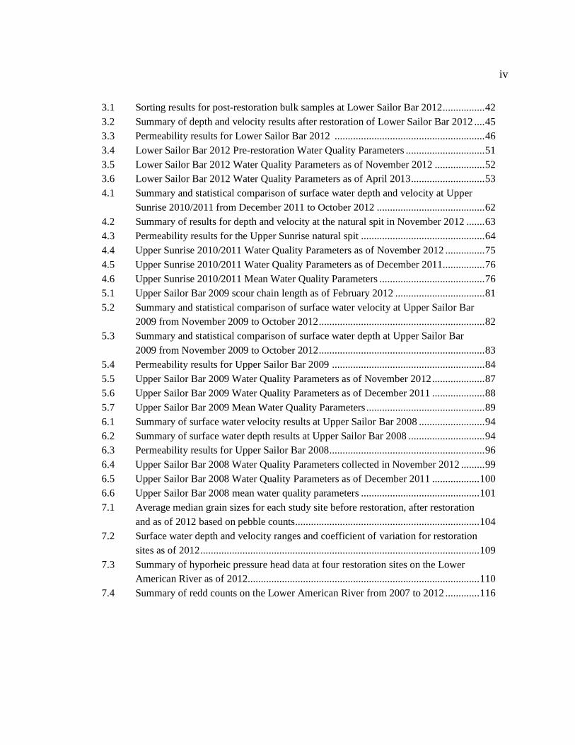
iv

3.1 Sorting results for post-restoration bulk samples at Lower Sailor Bar 2012 ................ 42

3.2 Summary of depth and velocity results after restoration of Lower Sailor Bar 2012 .... 45

3.3 Permeability results for Lower Sailor Bar 2012 ......................................................... 46

3.4 Lower Sailor Bar 2012 Pre-restoration Water Quality Parameters .............................. 51

3.5 Lower Sailor Bar 2012 Water Quality Parameters as of November 2012 ................... 52

3.6 Lower Sailor Bar 2012 Water Quality Parameters as of April 2013 ............................ 53

4.1 Summary and statistical comparison of surface water depth and velocity at Upper

Sunrise 2010/2011 from December 2011 to October 2012 ......................................... 62

4.2 Summary of results for depth and velocity at the natural spit in November 2012 ....... 63

4.3 Permeability results for the Upper Sunrise natural spit ............................................... 64

4.4 Upper Sunrise 2010/2011 Water Quality Parameters as of November 2012 ............... 75

4.5 Upper Sunrise 2010/2011 Water Quality Parameters as of December 2011................ 76

4.6 Upper Sunrise 2010/2011 Mean Water Quality Parameters ........................................ 76

5.1 Upper Sailor Bar 2009 scour chain length as of February 2012 .................................. 81

5.2 Summary and statistical comparison of surface water velocity at Upper Sailor Bar

2009 from November 2009 to October 2012 ............................................................... 82

5.3 Summary and statistical comparison of surface water depth at Upper Sailor Bar

2009 from November 2009 to October 2012 ............................................................... 83

5.4 Permeability results for Upper Sailor Bar 2009 .......................................................... 84

5.5 Upper Sailor Bar 2009 Water Quality Parameters as of November 2012 .................... 87

5.6 Upper Sailor Bar 2009 Water Quality Parameters as of December 2011 .................... 88

5.7 Upper Sailor Bar 2009 Mean Water Quality Parameters ............................................. 89

6.1 Summary of surface water velocity results at Upper Sailor Bar 2008 ......................... 94

6.2 Summary of surface water depth results at Upper Sailor Bar 2008 ............................. 94

6.3 Permeability results for Upper Sailor Bar 2008 ........................................................... 96

6.4 Upper Sailor Bar 2008 Water Quality Parameters collected in November 2012 ......... 99

6.5 Upper Sailor Bar 2008 Water Quality Parameters as of December 2011 .................. 100

6.6 Upper Sailor Bar 2008 mean water quality parameters ............................................. 101

7.1 Average median grain sizes for each study site before restoration, after restoration

and as of 2012 based on pebble counts...................................................................... 104

7.2 Surface water depth and velocity ranges and coefficient of variation for restoration

sites as of 2012 .......................................................................................................... 109

7.3 Summary of hyporheic pressure head data at four restoration sites on the Lower

American River as of 2012........................................................................................ 110

7.4 Summary of redd counts on the Lower American River from 2007 to 2012 ............. 116

v

LIST OF FIGURES

Figures Page

1.1 Longitudinal cross section of a pool-riffle sequence ..................................................... 3

1.2 Longitudinal cross section of a salmonid redd .............................................................. 3

1.3 Flow through a pool-riffle sequence .............................................................................. 4

1.4 Location map of Lower American River Restoration Project........................................ 6

1.5 Lower American River Peak Discharge from July 2008 through April 2013 ................ 8

1.6 Location of four restoration sites on the American River .............................................. 9

1.7 Front-end loaders placing gravel at the Lower Sailor Bar 2012 restoration site ............ 9

2.1 Salmonid spawning behavior ...................................................................................... 11

2.2 Lower Sailor Bar 2012 site with post-restoration pebble count transects .................... 12

2.3 Bulk sample collection at the Lower Sailor Bar 2012 site. .......................................... 14

2.4 Percent distribution for Lower Sailor Bar 2012 post-restoration bulk samples ........... 15

2.5 Tracer rocks initial placement and displacement after a high flow event .................... 17

2.6 Diagram of a scour chain with anchor constructed from pipe fittings. ........................ 17

2.7 Schematic of scour chains before and after a scour and fill events .............................. 18

2.8 Field team determining surface water depth and velocity .......................................... .20

2.9 Modified Terhune Mark IV standpipe schematic ........................................................ 22

2.10 Standpipe drawdown testing equipment and procedure. ............................................. 24

2.11 Modified Terhune (1958) calibration chart ................................................................. 25

2.12 Subsurface flow through gravel bed ............................................................................ 26

2.13 Hyporheic pressure head equipment ........................................................................... 27

2.14 Stream flow and temperature histories for a gaining and losing stream ...................... 29

2.15 Temperature logging equipment ................................................................................. 30

2.16 Conceptual model of flow through a pool tailout/riffle sequence ................................ 33

2.17 Cross section of hyporheic water quality measurements ............................................. 33

3.1 Pre-restoration pebble count traces at Lower Sailor Bar 2012..................................... 35

3.2 Post-restoration pebble count traces at Lower Sailor Bar 2012 ................................... 35

3.3 Pre-restoration pebble counts for the Lower Sailor Bar 2012 site ............................... 36

3.4 Post-restoration pebble counts for the Lower Sailor bar 2012 site .............................. 36

3.5 Lower Sailor Bar 2012 average pebble distribution before and after restoration ......... 37

3.6 Pebble count averages at Lower Sailor Bar 2012 ........................................................ 37

3.7 Post-restoration pebble count average compared to fine, medium and coarse patches

of material at Lower Sailor Bar 2012 .......................................................................... 38

3.8 Map of the Lower American River (modified from Snider et al., 1992) ..................... 39

3.9 Location of post-restoration bulk samples at Lower Sailor Bar 2012 .......................... 40

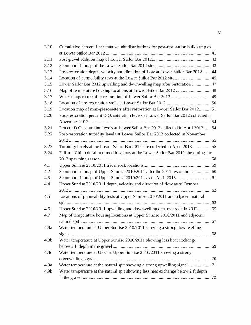
vi

3.10 Cumulative percent finer than weight distributions for post-restoration bulk samples

at Lower Sailor Bar 2012 ............................................................................................ 41

3.11 Post gravel addition map of Lower Sailor Bar 2012.. .................................................. 42

3.12 Scour and fill map of the Lower Sailor Bar 2012 site. ................................................ 43

3.13 Post-restoration depth, velocity and direction of flow at Lower Sailor Bar 2012 ....... 44

3.14 Location of permeability tests at the Lower Sailor Bar 2012 site ................................ 45

3.15 Lower Sailor Bar 2012 upwelling and downwelling map after restoration ................. 47

3.16 Map of temperature housing locations at Lower Sailor Bar 2012 ............................... 48

3.17 Water temperature after restoration of Lower Sailor Bar 2012 .................................... 49

3.18 Location of pre-restoration wells at Lower Sailor Bar 2012 ........................................ 50

3.19 Location map of mini-piezometers after restoration at Lower Sailor Bar 2012 ........... 51

3.20 Post-restoration percent D.O. saturation levels at Lower Sailor Bar 2012 collected in

November 2012 ........................................................................................................... 54

3.21 Percent D.O. saturation levels at Lower Sailor Bar 2012 collected in April 2013 ....... 54

3.22 Post-restoration turbidity levels at Lower Sailor Bar 2012 collected in November

2012 ............................................................................................................................ 55

3.23 Turbidity levels at the Lower Sailor Bar 2012 site collected in April 2013 ................. 55

3.24 Fall-run Chinook salmon redd locations at the Lower Sailor Bar 2012 site during the

2012 spawning season ................................................................................................. 58

4.1 Upper Sunrise 2010/2011 tracer rock locations ........................................................... 59

4.2 Scour and fill map of Upper Sunrise 2010/2011 after the 2011 restoration ................. 60

4.3 Scour and fill map of Upper Sunrise 2010/2011 as of April 2013 ............................... 61

4.4 Upper Sunrise 2010/2011 depth, velocity and direction of flow as of October

2012 ............................................................................................................................ 62

4.5 Locations of permeability tests at Upper Sunrise 2010/2011 and adjacent natural

spit .............................................................................................................................. 63

4.6 Upper Sunrise 2010/2011 upwelling and downwelling data recorded in 2012 ............ 65

4.7 Map of temperature housing locations at Upper Sunrise 2010/2011 and adjacent

natural spit................................................................................................................... 67

4.8a Water temperature at Upper Sunrise 2010/2011 showing a strong downwelling

signal ........................................................................................................................... 68

4.8b Water temperature at Upper Sunrise 2010/2011 showing less heat exchange

below 2 ft depth in the gravel ...................................................................................... 69

4.8c Water temperature at US-5 at Upper Sunrise 2010/2011 showing a strong

downwelling signal ..................................................................................................... 70

4.9a Water temperature at the natural spit showing a strong upwelling signal ................... .71

4.9b Water temperature at the natural spit showing less heat exchange below 2 ft depth

in the gravel ................................................................................................................ 72

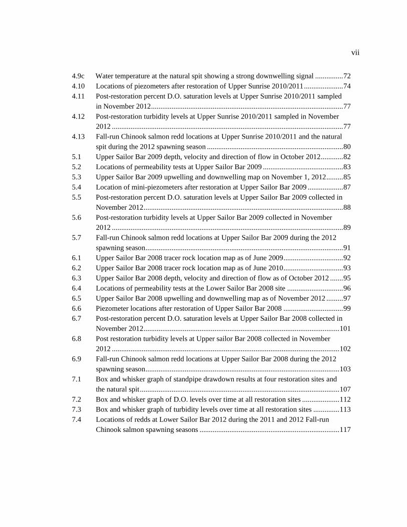
vii

4.9c Water temperature at the natural spit showing a strong downwelling signal ............... 72

4.10 Locations of piezometers after restoration of Upper Sunrise 2010/2011 ..................... 74

4.11 Post-restoration percent D.O. saturation levels at Upper Sunrise 2010/2011 sampled

in November 2012 ....................................................................................................... 77

4.12 Post-restoration turbidity levels at Upper Sunrise 2010/2011 sampled in November

2012 ............................................................................................................................ 77

4.13 Fall-run Chinook salmon redd locations at Upper Sunrise 2010/2011 and the natural

spit during the 2012 spawning season ......................................................................... 80

5.1 Upper Sailor Bar 2009 depth, velocity and direction of flow in October 2012 ............ 82

5.2 Locations of permeability tests at Upper Sailor Bar 2009 ........................................... 83

5.3 Upper Sailor Bar 2009 upwelling and downwelling map on November 1, 2012 ......... 85

5.4 Location of mini-piezometers after restoration at Upper Sailor Bar 2009 ................... 87

5.5 Post-restoration percent D.O. saturation levels at Upper Sailor Bar 2009 collected in

November 2012 ........................................................................................................... 88

5.6 Post-restoration turbidity levels at Upper Sailor Bar 2009 collected in November

2012 ............................................................................................................................ 89

5.7 Fall-run Chinook salmon redd locations at Upper Sailor Bar 2009 during the 2012

spawning season .......................................................................................................... 91

6.1 Upper Sailor Bar 2008 tracer rock location map as of June 2009 ................................ 92

6.2 Upper Sailor Bar 2008 tracer rock location map as of June 2010 ................................ 93

6.3 Upper Sailor Bar 2008 depth, velocity and direction of flow as of October 2012 ....... 95

6.4 Locations of permeability tests at the Lower Sailor Bar 2008 site .............................. 96

6.5 Upper Sailor Bar 2008 upwelling and downwelling map as of November 2012 ......... 97

6.6 Piezometer locations after restoration of Upper Sailor Bar 2008 ................................ 99

6.7 Post-restoration percent D.O. saturation levels at Upper Sailor Bar 2008 collected in

November 2012 ......................................................................................................... 101

6.8 Post restoration turbidity levels at Upper sailor Bar 2008 collected in November

2012 .......................................................................................................................... 102

6.9 Fall-run Chinook salmon redd locations at Upper Sailor Bar 2008 during the 2012

spawning season ........................................................................................................ 103

7.1 Box and whisker graph of standpipe drawdown results at four restoration sites and

the natural spit ........................................................................................................... 107

7.2 Box and whisker graph of D.O. levels over time at all restoration sites .................... 112

7.3 Box and whisker graph of turbidity levels over time at all restoration sites .............. 113

7.4 Locations of redds at Lower Sailor Bar 2012 during the 2011 and 2012 Fall-run

Chinook salmon spawning seasons ........................................................................... 117

1

1.0 INTRODUCTION

Anthropogenic forces, including dams, artificial levees, channel modification and

overall urbanization have been shown to limit the quantity and quality of available

spawning gravel necessary for anadromous salmonid populations in rivers (Vyverberg et

al., 1997; Phillips, 2003; Hannon and Deason, 2005). These forces lead to streambed

degradation, a primary factor in the continued decline of resident salmonid populations in

the Lower American River (Horner, 2004; Kondolf et al., 2008). In response to this

problem, a multi-phase remediation project was conducted on the river as part of the

Central Valley Project Improvement Act of 1992 (CVPIA section b.13) which mandates

the improvement of gravel conditions below federal dams. Project collaborators included

California State University Sacramento (CSUS), U.S. Bureau of Reclamation (BOR),

Sacramento Water Forum, U.S. Fish and Wildlife Service, CBEC consultants, NOAA

Fisheries, and Cramer Fish Sciences.

1.1 OBJECTIVES

This report is a summary of hydrologic and physical data collected at four

restoration sites on the Lower American River: Upper Sailor Bar 2008, Upper Sailor Bar

2009, Upper Sunrise 2010/2011, and Lower Sailor Bar 2012. Data was collected before

and after restoration of each site, and in subsequent years. Analysis includes an

assessment of temporal changes at individual sites and a comprehensive comparison of

results between all four sites. Field work and analyses conducted during the 2012/2013

field season fulfilled seven major objectives, described as tasks in a gravel monitoring

proposal submitted to the U.S. Bureau of Reclamation, Sacramento office on July 9,

2012. The tasks are summarized below:

(1) Conduct grain size analyses using pebble counts and bulk samples

(2) Conduct gravel mobility tests and analysis using tracer rocks and scour chains

(3) Measure depth and velocity of surface water

(4) Measure gravel permeability with tracer tests

2

(5) Measure hyporheic pressure head of mini-piezometers vs. surface water (upwelling

and downwelling)

(6) Measure temperature data using temperature loggers

(7) Measure hyporheic water quality field parameters (dissolved oxygen, turbidity,

electrical conductivity, pH, and temperature) from mini-piezometers

1.2 BACKGROUND

Salmonid species are critical indicators of good water quality, a healthy

ecosystem, and effective watershed management (DeVries, 2000). Gravel-bed streams

are used by salmonids for spawning and the incubation of embryos. Approximately one

third of natural salmonid spawning in Northern California occurs in the Lower American

River, making the condition of this stream channel very important. The American River

has been the site of at least seven gravel experiments or augmentation projects over the

past 20 years (Vyverberg et al., 1997; Hannon 2000, Horner et al., 2004; Horner, 2005;

Redd and Horner, 2009; Janes et al., 2012). The focus of these projects has been gravel

addition or enhancement to offset the degradation of natural spawning areas on the river.

Many of the factors that limit successful natural spawning are part of the physical

environment and depend on appropriate water depth and velocity, substrate size,

temperature, dissolved oxygen content, and a variety of other more subtle factors like

cover, upwelling or downwelling conditions, and hyporheic flow.

Spawning Habitat Requirements

Naturally flowing gravel-bed streams are often characterized by changes in bed

gradient that appear as a series of pools and riffles. Pool-riffle sequences provide a

heterogeneous environment for salmonid spawning (Figure 1.1). Successful salmon

spawning occurs when the female salmon is able to construct a redd (spawning nest) by

excavating a pit in streambed gravel, deposit and bury her eggs, the eggs incubate and

hatch, and alevins (recently hatched fish) develop and emerge (Kondolf et al., 2008).

3

Redd construction creates localized flow conditions that direct stream flow through

individual redds (Figure 1.2).

Figure 1.1: Longitudinal cross section of a pool-riffle sequence. (From FSC, 2012)

Figure 1.2: Longitudinal cross section of a salmonid redd. Depicted are the original bed

surface elevation (dashed line), locations of two egg pockets, and disturbed bed material

(shaded particles) forming a tailspill. (From DeVries, 2000)

Salmonids construct redds between 7 in and 12 in deep in the streambed (Hannon,

2000; Monaghan and Milner, 2009) and bury their eggs in the hyporheic zone. The

hyporheic zone is the band of shallow gravel where exchange occurs between the stream

and the subsurface (Bencala, 2005). This active interface between groundwater and

surface water is important for the supply of chemicals, nutrients and organic matter that

characterize a healthy ecosystem. Dynamic flow through the hyporheic zone supplies

oxygenated water to egg pockets while removing metabolic waste (Coble, 1961; Vaux,

1962; Chevalier et al., 1984).

Egg pockets

Flow

4

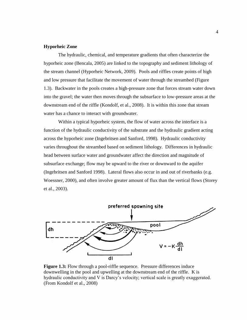
Hyporheic Zone

The hydraulic, chemical, and temperature gradients that often characterize the

hyporheic zone (Bencala, 2005) are linked to the topography and sediment lithology of

the stream channel (Hyporheic Network, 2009). Pools and riffles create points of high

and low pressure that facilitate the movement of water through the streambed (Figure

1.3). Backwater in the pools creates a high-pressure zone that forces stream water down

into the gravel; the water then moves through the subsurface to low-pressure areas at the

downstream end of the riffle (Kondolf, et al., 2008). It is within this zone that stream

water has a chance to interact with groundwater.

Within a typical hyporheic system, the flow of water across the interface is a

function of the hydraulic conductivity of the substrate and the hydraulic gradient acting

across the hyporheic zone (Ingebritsen and Sanford, 1998). Hydraulic conductivity

varies throughout the streambed based on sediment lithology. Differences in hydraulic

head between surface water and groundwater affect the direction and magnitude of

subsurface exchange; flow may be upward to the river or downward to the aquifer

(Ingebritsen and Sanford 1998). Lateral flows also occur in and out of riverbanks (e.g.

Woessner, 2000), and often involve greater amount of flux than the vertical flows (Storey

et al., 2003).

Figure 1.3: Flow through a pool-riffle sequence. Pressure differences induce

downwelling in the pool and upwelling at the downstream end of the riffle. K is

hydraulic conductivity and V is Darcy’s velocity; vertical scale is greatly exaggerated.

(From Kondolf et al., 2008)

5

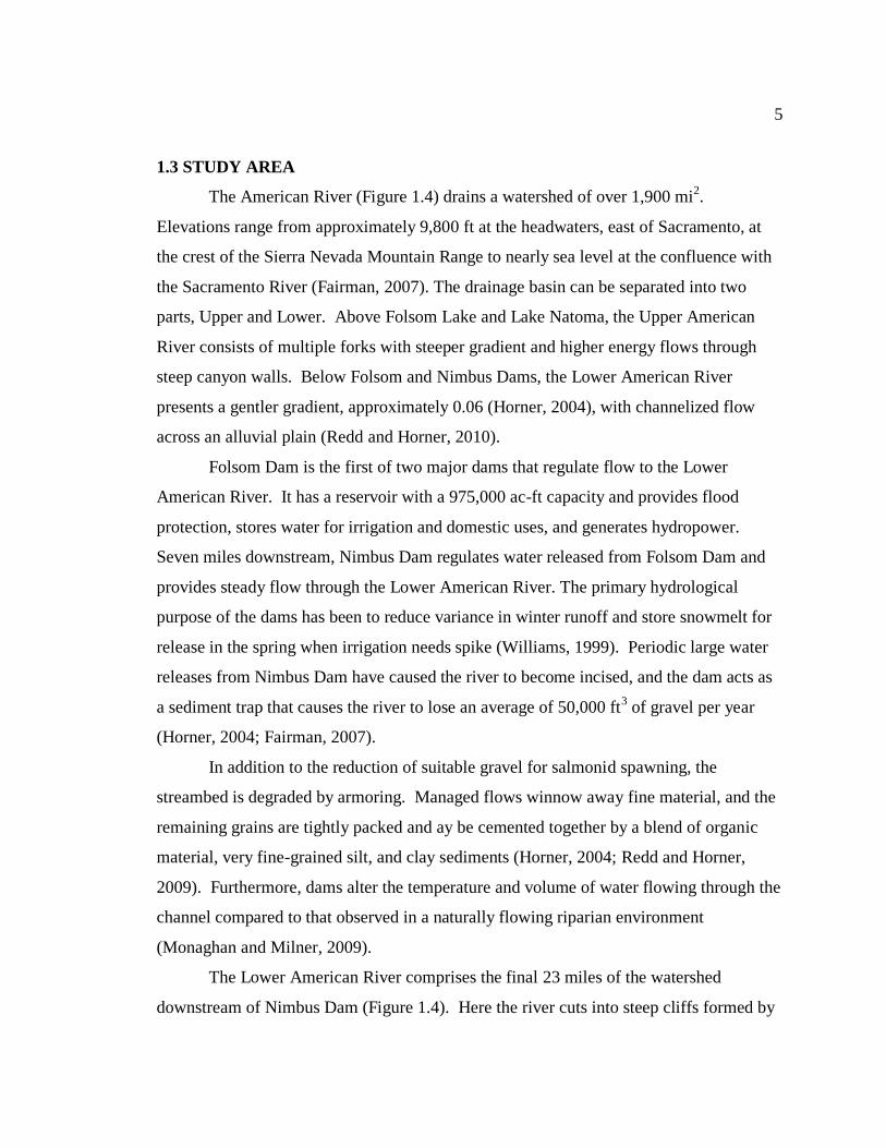
1.3 STUDY AREA

The American River (Figure 1.4) drains a watershed of over 1,900 mi2.

Elevations range from approximately 9,800 ft at the headwaters, east of Sacramento, at

the crest of the Sierra Nevada Mountain Range to nearly sea level at the confluence with

the Sacramento River (Fairman, 2007). The drainage basin can be separated into two

parts, Upper and Lower. Above Folsom Lake and Lake Natoma, the Upper American

River consists of multiple forks with steeper gradient and higher energy flows through

steep canyon walls. Below Folsom and Nimbus Dams, the Lower American River

presents a gentler gradient, approximately 0.06 (Horner, 2004), with channelized flow

across an alluvial plain (Redd and Horner, 2010).

Folsom Dam is the first of two major dams that regulate flow to the Lower

American River. It has a reservoir with a 975,000 ac-ft capacity and provides flood

protection, stores water for irrigation and domestic uses, and generates hydropower.

Seven miles downstream, Nimbus Dam regulates water released from Folsom Dam and

provides steady flow through the Lower American River. The primary hydrological

purpose of the dams has been to reduce variance in winter runoff and store snowmelt for

release in the spring when irrigation needs spike (Williams, 1999). Periodic large water

releases from Nimbus Dam have caused the river to become incised, and the dam acts as

a sediment trap that causes the river to lose an average of 50,000 ft3 of gravel per year

(Horner, 2004; Fairman, 2007).

In addition to the reduction of suitable gravel for salmonid spawning, the

streambed is degraded by armoring. Managed flows winnow away fine material, and the

remaining grains are tightly packed and ay be cemented together by a blend of organic

material, very fine-grained silt, and clay sediments (Horner, 2004; Redd and Horner,

2009). Furthermore, dams alter the temperature and volume of water flowing through the

channel compared to that observed in a naturally flowing riparian environment

(Monaghan and Milner, 2009).

The Lower American River comprises the final 23 miles of the watershed

downstream of Nimbus Dam (Figure 1.4). Here the river cuts into steep cliffs formed by

6

Miocene to Pliocene-aged sandstone and siltstone of the Fair Oaks and Mehrten

Formations (Schlemon, 1967). The riverbed substrate becomes progressively smaller as

it meets its terminus with the Sacramento River, moving from coarse-grained gravels to

smaller sand and silt sized material (Vyverberg et al. 1997). The river’s south bank is

composed of gradually terraced Pleistocene alluvial gravels (Schlemon, 1967). The study

area for this report includes four reaches located approximately one mile downstream of

Nimbus Dam (Figure 1.4).

Figure 1.4: Location map of Lower American River Restoration Project

The regional climate is Mediterranean, characterized by warm, dry summers and

cool, wet winters. Average precipitation in the watershed ranges from 18.5 in/yr to 78.7

7

in/yr (NOAA, 2011). Stream flow is highly seasonal (USGS, 2009). Lower elevation

run-off is the result of winter rains, and very high flows are the result of winter storms

(Williams, 1999). Prior to 1955 (year of completion of Folsom and Nimbus Dams),

American River peak flows ranged from 10,000 cfs to180,000 cfs; current annual peak

flow ranges between 1,000 cfs and 135,000 cfs (USGS, 2009). Daily peak flows during

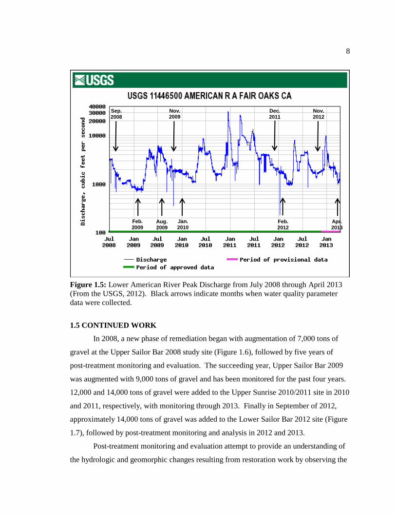
the duration of this study (2008-2013), ranged from 1,000 cfs to 30,000 cfs (Figure 1.5).

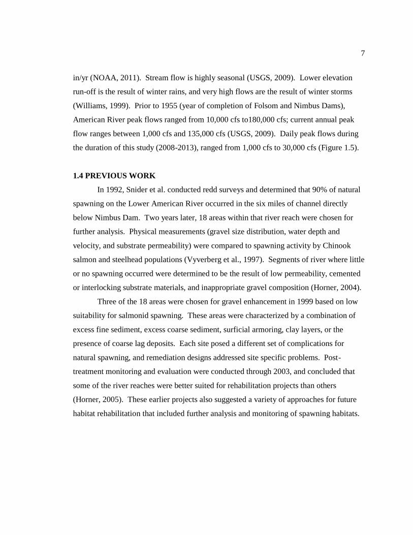
1.4 PREVIOUS WORK

In 1992, Snider et al. conducted redd surveys and determined that 90% of natural

spawning on the Lower American River occurred in the six miles of channel directly

below Nimbus Dam. Two years later, 18 areas within that river reach were chosen for

further analysis. Physical measurements (gravel size distribution, water depth and

velocity, and substrate permeability) were compared to spawning activity by Chinook

salmon and steelhead populations (Vyverberg et al., 1997). Segments of river where little

or no spawning occurred were determined to be the result of low permeability, cemented

or interlocking substrate materials, and inappropriate gravel composition (Horner, 2004).

Three of the 18 areas were chosen for gravel enhancement in 1999 based on low

suitability for salmonid spawning. These areas were characterized by a combination of

excess fine sediment, excess coarse sediment, surficial armoring, clay layers, or the

presence of coarse lag deposits. Each site posed a different set of complications for

natural spawning, and remediation designs addressed site specific problems. Post-

treatment monitoring and evaluation were conducted through 2003, and concluded that

some of the river reaches were better suited for rehabilitation projects than others

(Horner, 2005). These earlier projects also suggested a variety of approaches for future

habitat rehabilitation that included further analysis and monitoring of spawning habitats.

8

Figure 1.5: Lower American River Peak Discharge from July 2008 through April 2013

(From the USGS, 2012). Black arrows indicate months when water quality parameter

data were collected.

1.5 CONTINUED WORK

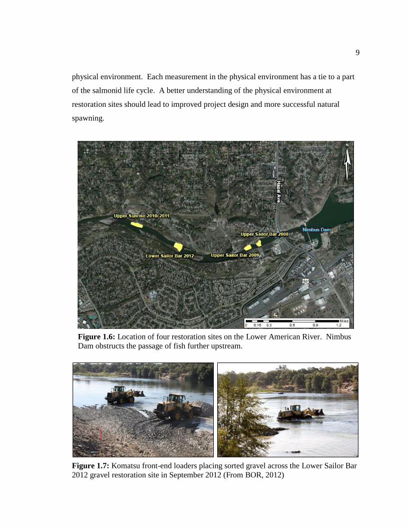
In 2008, a new phase of remediation began with augmentation of 7,000 tons of

gravel at the Upper Sailor Bar 2008 study site (Figure 1.6), followed by five years of

post-treatment monitoring and evaluation. The succeeding year, Upper Sailor Bar 2009

was augmented with 9,000 tons of gravel and has been monitored for the past four years.

12,000 and 14,000 tons of gravel were added to the Upper Sunrise 2010/2011 site in 2010

and 2011, respectively, with monitoring through 2013. Finally in September of 2012,

approximately 14,000 tons of gravel was added to the Lower Sailor Bar 2012 site (Figure

1.7), followed by post-treatment monitoring and analysis in 2012 and 2013.

Post-treatment monitoring and evaluation attempt to provide an understanding of

the hydrologic and geomorphic changes resulting from restoration work by observing the

Sep.

2008

Feb.

2009

Nov. 2009

Jan.

2010 Feb.

2012

Dec.

2011

Nov.

2012

Apr.

2013

Aug.

2009

9

physical environment. Each measurement in the physical environment has a tie to a part

of the salmonid life cycle. A better understanding of the physical environment at

restoration sites should lead to improved project design and more successful natural

spawning.

Figure 1.6: Location of four restoration sites on the Lower American River. Nimbus

Dam obstructs the passage of fish further upstream.

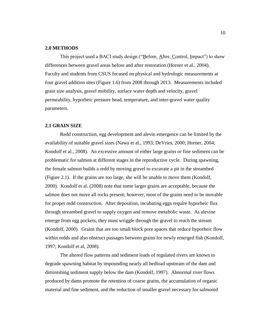
Figure 1.7: Komatsu front-end loaders placing sorted gravel across the Lower Sailor Bar

2012 gravel restoration site in September 2012 (From BOR, 2012)

10

2.0 METHODS

This project used a BACI study design (“Before, After, Control, Impact”) to show

differences between gravel areas before and after restoration (Horner et al., 2004).

Faculty and students from CSUS focused on physical and hydrologic measurements at

four gravel addition sites (Figure 1.6) from 2008 through 2013. Measurements included

grain size analysis, gravel mobility, surface water depth and velocity, gravel

permeability, hyporheic pressure head, temperature, and inter-gravel water quality

parameters.

2.1 GRAIN SIZE

Redd construction, egg development and alevin emergence can be limited by the

availability of suitable gravel sizes (Nawa et al., 1993; DeVries, 2000; Horner, 2004;

Kondolf et al., 2008). An excessive amount of either large grains or fine sediment can be

problematic for salmon at different stages in the reproductive cycle. During spawning,

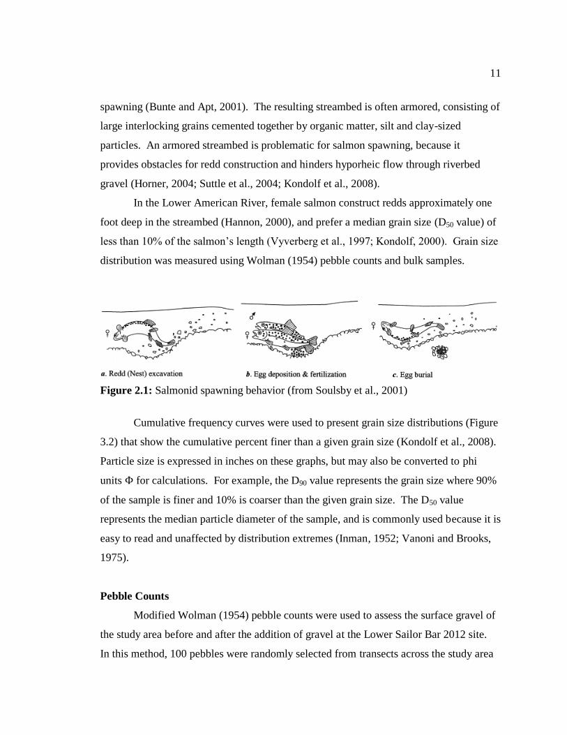
the female salmon builds a redd by moving gravel to excavate a pit in the streambed

(Figure 2.1). If the grains are too large, she will be unable to move them (Kondolf,

2000). Kondolf et al. (2008) note that some larger grains are acceptable, because the

salmon does not move all rocks present; however, most of the grains need to be movable

for proper redd construction. After deposition, incubating eggs require hyporheic flux

through streambed gravel to supply oxygen and remove metabolic waste. As alevine

emerge from egg pockets, they must wriggle through the gravel to reach the stream

(Kondolf, 2000). Grains that are too small block pore spaces that reduce hyporheic flow

within redds and also obstruct passages between grains for newly emerged fish (Kondolf,

1997; Kondolf et al, 2008).

The altered flow patterns and sediment loads of regulated rivers are known to

degrade spawning habitat by impounding nearly all bedload upstream of the dam and

diminishing sediment supply below the dam (Kondolf, 1997). Abnormal river flows

produced by dams promote the retention of coarse grains, the accumulation of organic

material and fine sediment, and the reduction of smaller gravel necessary for salmonid

11

spawning (Bunte and Apt, 2001). The resulting streambed is often armored, consisting of

large interlocking grains cemented together by organic matter, silt and clay-sized

particles. An armored streambed is problematic for salmon spawning, because it

provides obstacles for redd construction and hinders hyporheic flow through riverbed

gravel (Horner, 2004; Suttle et al., 2004; Kondolf et al., 2008).

In the Lower American River, female salmon construct redds approximately one

foot deep in the streambed (Hannon, 2000), and prefer a median grain size (D50 value) of

less than 10% of the salmon’s length (Vyverberg et al., 1997; Kondolf, 2000). Grain size

distribution was measured using Wolman (1954) pebble counts and bulk samples.

Figure 2.1: Salmonid spawning behavior (from Soulsby et al., 2001)

Cumulative frequency curves were used to present grain size distributions (Figure

3.2) that show the cumulative percent finer than a given grain size (Kondolf et al., 2008).

Particle size is expressed in inches on these graphs, but may also be converted to phi

units for calculations. For example, the D90 value represents the grain size where 90%

of the sample is finer and 10% is coarser than the given grain size. The D50 value

represents the median particle diameter of the sample, and is commonly used because it is

easy to read and unaffected by distribution extremes (Inman, 1952; Vanoni and Brooks,

1975).

Pebble Counts

Modified Wolman (1954) pebble counts were used to assess the surface gravel of

the study area before and after the addition of gravel at the Lower Sailor Bar 2012 site.

In this method, 100 pebbles were randomly selected from transects across the study area

12

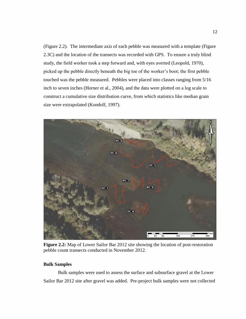
(Figure 2.2). The intermediate axis of each pebble was measured with a template (Figure

2.3C) and the location of the transects was recorded with GPS. To ensure a truly blind

study, the field worker took a step forward and, with eyes averted (Leopold, 1970),

picked up the pebble directly beneath the big toe of the worker’s boot; the first pebble

touched was the pebble measured. Pebbles were placed into classes ranging from 5/16

inch to seven inches (Horner et al., 2004), and the data were plotted on a log scale to

construct a cumulative size distribution curve, from which statistics like median grain

size were extrapolated (Kondolf, 1997).

Figure 2.2: Map of Lower Sailor Bar 2012 site showing the location of post-restoration

pebble count transects conducted in November 2012.

Bulk Samples

Bulk samples were used to assess the surface and subsurface gravel at the Lower

Sailor Bar 2012 site after gravel was added. Pre-project bulk samples were not collected

13

because of high flows and deep water at the site. This method considers fine sediments

within the substrate that are not accounted for by pebble counts. In this method, a marker

was tossed to randomly determine the center of the bulk sample area, and the location

was mapped using GPS. Bulk sample size was calculated by multiplying the weight of

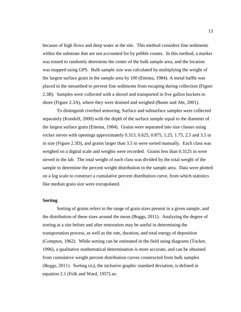
the largest surface grain in the sample area by 100 (Ettema, 1984). A metal baffle was

placed in the streambed to prevent fine sediments from escaping during collection (Figure

2.3B). Samples were collected with a shovel and transported in five gallon buckets to

shore (Figure 2.3A), where they were drained and weighed (Bunte and Abt, 2001).

To distinguish riverbed armoring, Surface and subsurface samples were collected

separately (Kondolf, 2000) with the depth of the surface sample equal to the diameter of

the largest surface grain (Ettema, 1984). Grains were separated into size classes using

rocker sieves with openings approximately 0.313, 0.625, 0.875, 1.25, 1.75, 2.5 and 3.5 in

in size (Figure 2.3D), and grains larger than 3.5 in were sorted manually. Each class was

weighed on a digital scale and weights were recorded. Grains less than 0.3125 in were

sieved in the lab. The total weight of each class was divided by the total weight of the

sample to determine the percent weight distribution in the sample area. Data were plotted

on a log scale to construct a cumulative percent distribution curve, from which statistics

like median grain size were extrapolated.

Sorting

Sorting of grains refers to the range of grain sizes present in a given sample, and

the distribution of these sizes around the mean (Boggs, 2011). Analyzing the degree of

sorting at a site before and after restoration may be useful in determining the

transportation process, as well as the rate, duration, and total energy of deposition

(Compton, 1962). While sorting can be estimated in the field using diagrams (Tucker,

1996), a qualitative mathematical determination is more accurate, and can be obtained

from cumulative weight percent distribution curves constructed from bulk samples

(Boggs, 2011). Sorting (σi), the inclusive graphic standard deviation, is defined in

equation 2.1 (Folk and Ward, 1957) as:

14

σi = 84 – 16 95 – 5 (2.1)

4 6.6

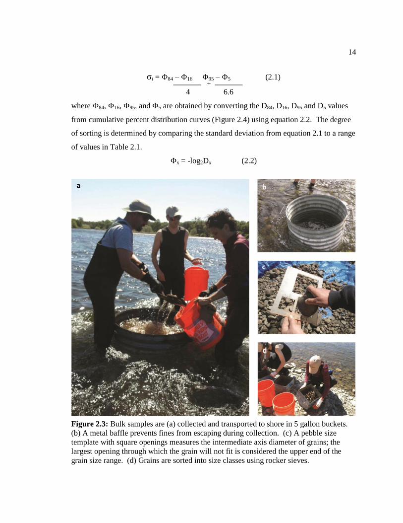
where 84, 16, 95, and 5 are obtained by converting the D84, D16, D95 and D5 values

from cumulative percent distribution curves (Figure 2.4) using equation 2.2. The degree

of sorting is determined by comparing the standard deviation from equation 2.1 to a range

of values in Table 2.1.

x = -log2Dx (2.2)

Figure 2.3: Bulk samples are (a) collected and transported to shore in 5 gallon buckets.

(b) A metal baffle prevents fines from escaping during collection. (c) A pebble size

template with square openings measures the intermediate axis diameter of grains; the

largest opening through which the grain will not fit is considered the upper end of the

grain size range. (d) Grains are sorted into size classes using rocker sieves.

a b

c

d

_______ + _______

15

Figure 2.4: Cumulative percent distribution curve for grain size (measured in phi) at the

Lower Sailor Bar 2012 site (post-restoration) from bulk sample data. D84, D16, D95, and

D5 values are noted in red.

Table 2.1: Standard deviation range and degree of sorting (From Boggs, 2011)

Standard Deviation Sorting

< 0.35 Very well sorted

0.35-0.50 Well sorted

0.50-0.71 Moderately well sorted

0.71-1.00 Moderately sorted

1.00-2.00 Poorly sorted

2.00-4.00 Very poorly sorted

>4.00 Extremely poorly sorted

2.2 GRAVEL MOBILITY

Successful salmonid spawning can be impacted by gravel mobilization during

high stream flow events (Nawa et al., 1990; DeVries, 2000), because the rounded cobbles

and pebbles necessary for spawning are highly mobile. The movement of this material

has both biological and physical implications, so the effects of high flows on spawning

habitat are very important. Large magnitude flood events are capable of eroding and

0%

10%

20%

30%

40%

50%

60%

70%

80%

90%

100%

-8 -7 -6 -5 -4 -3 -2 -1

Cu

mm

ula

tive

Wei

ght

Per

cen

t

Grain Size (Φ)

Surface Sample 1

D95

D84 D16

D5

16

depositing streambed material over a short period of time, causing changes in bed

topography called scour and fill (Leopold, 1964). Scour and fill can lead to the complete

washout or crushing of salmonid eggs (DeVries, 1997). Some studies indicate that

salmonid embryo survival can be limited if a redd is scoured down to egg elevation

(McNeil 1966; Seegrist and Gard, 1972; Kondolf et al., 1991), while others have found

that even minor scour can significantly reduce the survival of embryos (Montgomery et

al., 1996).

Localized scour and fill are common at restoration sites on the Lower American

River, and problematic for the overall longevity of restoration projects (Horner, 2005).

Previous studies have shown that the processes of scour and fill are influenced by several

factors (Carling, 1987; Haschenberger, 1999; Bigelow, 2005; DeVries, 2000). Some

studies indicate that scour and fill are controlled by shear stress levels (Bigelow, 2005),

while others point to a correlation between sediment supply, particle size, and the amount

of scour and fill that occurs in the stream bed (Lisle and Eads, 1991; Nawa and Frissell,

1993; Harvey and Lisle, 1999; DeVries, 2000). Information about scour and fill will

inform managers about the average longevity of projects, and the intervals at which

gravel will need to be replenished. For this study, gravel mobility was measured using

tracer rocks and scour chains.

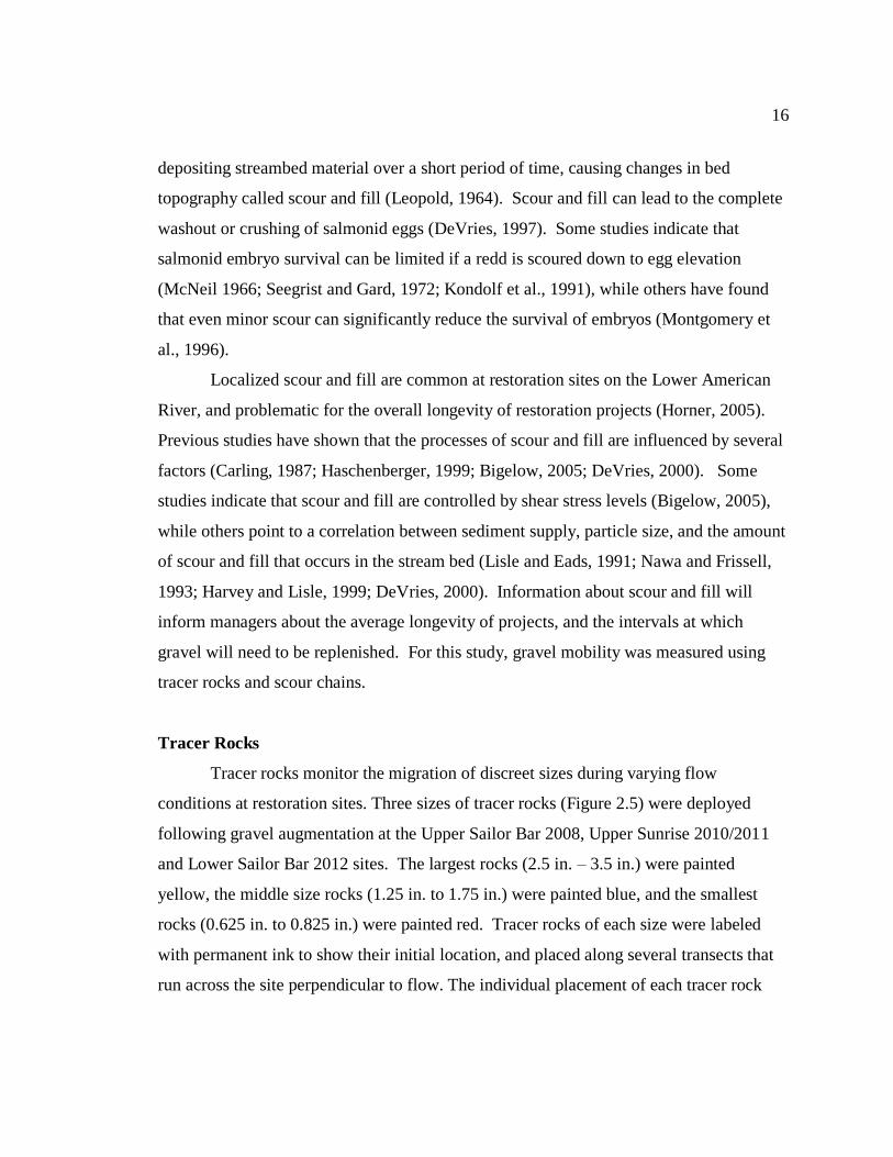
Tracer Rocks

Tracer rocks monitor the migration of discreet sizes during varying flow

conditions at restoration sites. Three sizes of tracer rocks (Figure 2.5) were deployed

following gravel augmentation at the Upper Sailor Bar 2008, Upper Sunrise 2010/2011

and Lower Sailor Bar 2012 sites. The largest rocks (2.5 in. – 3.5 in.) were painted

yellow, the middle size rocks (1.25 in. to 1.75 in.) were painted blue, and the smallest

rocks (0.625 in. to 0.825 in.) were painted red. Tracer rocks of each size were labeled

with permanent ink to show their initial location, and placed along several transects that

run across the site perpendicular to flow. The individual placement of each tracer rock

17

was mapped using GPS, and position of the tracer rocks was tracked after various flow

events.

Figure 2.5: (a) Initial placement of yellow, blue,

and red tracer rocks; (b) displacement of yellow

tracer rock following a higher flow event indicates

movement of bedload.

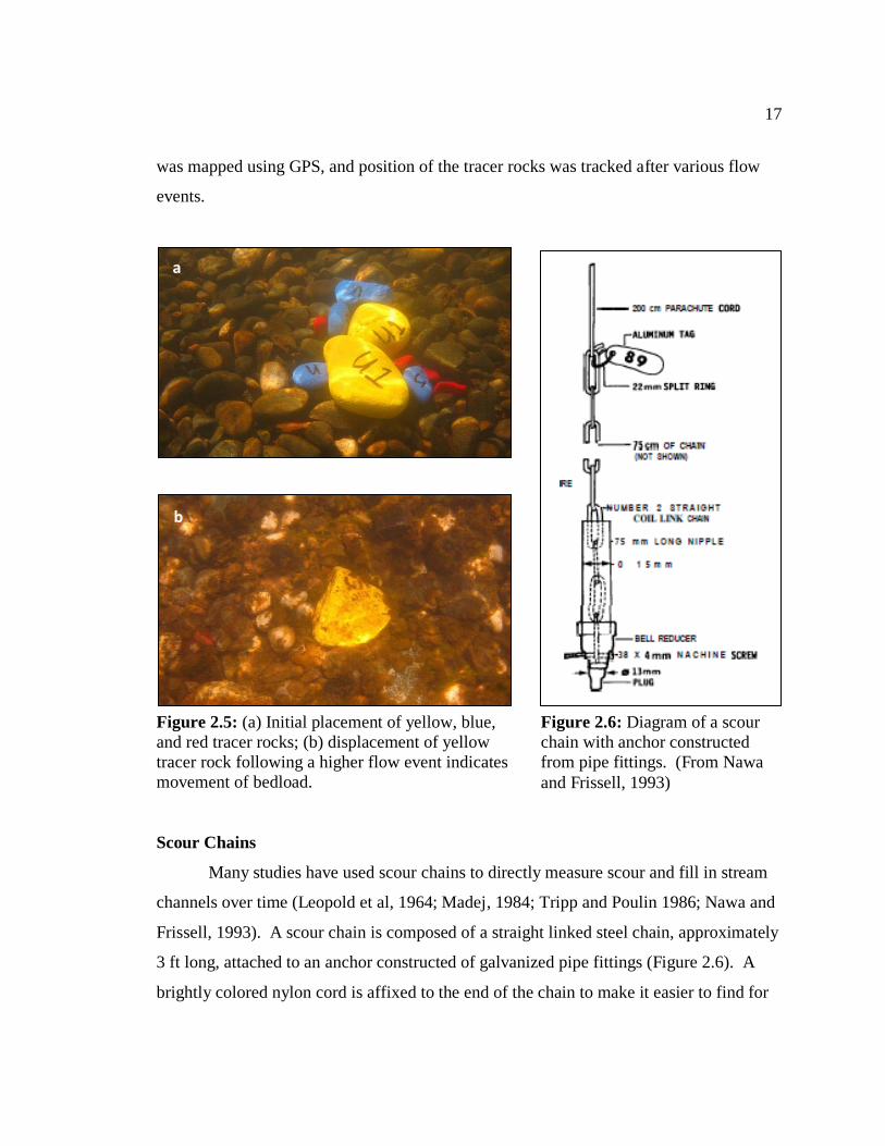
Scour Chains

Many studies have used scour chains to directly measure scour and fill in stream

channels over time (Leopold et al, 1964; Madej, 1984; Tripp and Poulin 1986; Nawa and

Frissell, 1993). A scour chain is composed of a straight linked steel chain, approximately

3 ft long, attached to an anchor constructed of galvanized pipe fittings (Figure 2.6). A

brightly colored nylon cord is affixed to the end of the chain to make it easier to find for

Figure 2.6: Diagram of a scour

chain with anchor constructed

from pipe fittings. (From Nawa

and Frissell, 1993)

b

a

18

future measurements. The completed scour chain is inserted approximately 15 in.- 20 in.

down into the streambed (anchor side down) using a steel pipe and a post driver.

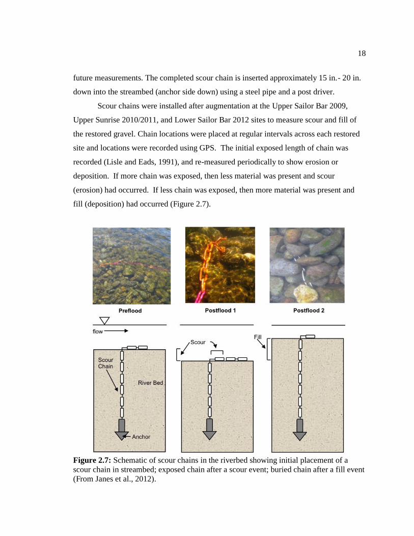
Scour chains were installed after augmentation at the Upper Sailor Bar 2009,

Upper Sunrise 2010/2011, and Lower Sailor Bar 2012 sites to measure scour and fill of

the restored gravel. Chain locations were placed at regular intervals across each restored

site and locations were recorded using GPS. The initial exposed length of chain was

recorded (Lisle and Eads, 1991), and re-measured periodically to show erosion or

deposition. If more chain was exposed, then less material was present and scour

(erosion) had occurred. If less chain was exposed, then more material was present and

fill (deposition) had occurred (Figure 2.7).

Figure 2.7: Schematic of scour chains in the riverbed showing initial placement of a

scour chain in streambed; exposed chain after a scour event; buried chain after a fill event

(From Janes et al., 2012).

19

2.3 SURFACE WATER DEPTH AND VELOCITY

Surface water depth and velocity are key factors in the selection of suitable redd

sites by spawning salmonids. If velocities are too high, the female salmon must expend

excessive amounts of energy fighting the current and spends less time on her redd when

compared to optimal conditions (Chapman et al., 1986, Hannon, 2000). If velocities are

too low, hyporheic exchange is lessened and oxygen and nutrients are not delivered to the

developing eggs. In 2004, Horner et al. reported that optimal salmonid spawning in the

Lower American River occurred at water depths ranging from the fin height of the

salmon to approximately six feet of stream depth. Chapman et al. (1986) found that

Chinook salmon prefer water velocities between 1.3 ft/sec. and 6.3 ft/sec.

Depth and velocity were measured at all four restoration site using standard

USGS stream gaging procedures (1980). A topset wading rod was used to determine

depth. A Price AA current meter or a Marsh-McBirney electronic velocity meter was

attached to the wading rod to measure surface water velocities (Figure 2.8).

Measurements were made at locations where mini-piezometers had been installed

throughout the study area. When using the current meter, the number of revolutions (R)

completed by current meter cups was counted for a 60 second interval, and then

converted to velocity (V) using equation 2.2 (USGS, 1980).

V=2.2048(R)+0.0178 (2.2)

The Marsh-McBirney electronic velocity meter automatically calculated a velocity value

in feet per second. Two velocity measurements were taken at each mini-piezometer

location, at 60% and 80% below the water surface. The 60% measurement represents the

average velocity of the water column, and the 80% measurement represents the “snout

velocity” of the salmonid. The direction of flow was measured using a Brunton compass.

Depth and Velocity data are reported on maps showing depth, velocity and

direction of flow, and in tables that include range, mean, standard deviation, and the

coefficient of variation. The coefficient of variation (CV) is a normalized measure of the

dispersion in a distribution that does not depend on the unit of a given parameter, in this

20

case depth and velocity. CV is a dimensionless value defined as the ratio of the standard

deviation (σ) to the mean ( ) multiplied by 100, as in equation 2.3 (Neville and Kennedy,

1964), and shows the extent of variability in relation to the mean: the higher the

coefficient, the greater the dispersion in the parameter. The CV can only be used if the

mean of a variable is not zero or close to zero, and if all sampled values are positive

(UCLA, 2013).

CV =

× 100 (2.3)

While standard deviation is a useful way to look at the dispersion of a single

variable, it is unit dependent and cannot be compared to variables with differing units in a

meaningful way. The advantage of the CV is that it is dimensionless. As a ratio of the

standard deviation and the mean (both of which are expressed in the same units, allowing

for the cancellation of units), CV’s of different variables (and differing units) can be

compared in a meaningful way: the variable with the greater CV is more dispersed than

the variable with the smaller CV (UCLA, 2013).

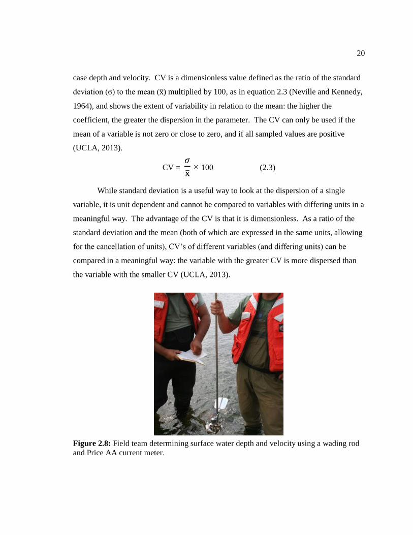
Figure 2.8: Field team determining surface water depth and velocity using a wading rod

and Price AA current meter.

21

2.4 GRAVEL PERMEABILITY

When eggs have been deposited in the redd, it is imperative that flow persist

through the streambed. The ability of water to move through hyporheic gravels, or

permeability, is used as an indicator of spawning gravel quality. Highly permeable

gravels allow the exchange of oxygenated water and other nutrients between the stream

channel and hyporheic zone (Barnard and McBain, 1994). When excess fine sediment

intrudes into the streambed, the decreased permeability effects this active exchange, and

can have negative effects on egg and fry survival (Cordone and Kelley 1961). According

to Terhune (1958), the survival of eggs is highly dependent on the oxygen available to

them in the surrounding water.

In past studies (Janes et al., 2012), gravel permeability was evaluated using

saltwater tracer tests to measure subsurface seepage velocities in the shallow gravel

where salmonids construct redds. Tracer Tests are dependent on stream flow, require

long field tests, and may cause swelling of clay minerals in the subsurface. Additionally,

tracer tests produce a seepage velocity that is not directly comparable to the hydraulic

conductivity (K) value that typically describes permeability. Because of these factors, it

was determined that standpipe drawdown tests (Terhune 1958; Barnard and McBain,

1994) are more effective at evaluating gravel permeability, and therefore standpipe

drawdown tests were conducted at all four restoration sites during the 2011/2012 field

season.

Standpipe Drawdown Test

Permeability was measured using the standpipe drawdown test, pioneer by

Terhune (1958) and adapted by Barnard and McBain (1994). In this method, a modified

Terhune Mark IV standpipe (Figure 2.9a) was inserted into the streambed, and a pumping

apparatus used to create a constant one inch drawdown in the intragravel water (Figure

2.9b). The volume of water collected during drawdown was measured and duration of

the test recorded.

22

The pumping apparatus was composed of two capture tanks with individual intake

valves attached to a vacuum pump and extraction hose (Figure 2.10a). One tank was

used to collect test water, and the other to collect residual water. Residual water was a

byproduct of the initial drawdown volume, and the water that drained out of the system

following the test. To clear the screen of debris and stabilize recorded measurements, the

pipe was developed before testing. To develop the standpipe, the extraction hose was

inserted into the standpipe and approximately five gallons of water removed. Water was

pumped from the standpipe until it was clear, indicating that silt and clay were removed

from the standpipe and screened area. In cases where this volume of water could not be

extracted, water was removed until turbidity was sufficiently low.

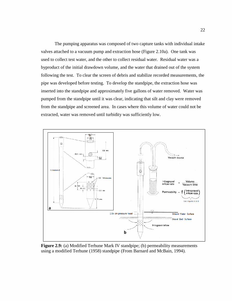
Figure 2.9: (a) Modified Terhune Mark IV standpipe; (b) permeability measurements

using a modified Terhune (1958) standpipe (From Barnard and McBain, 1994).

a

b

23

After the standpipe was appropriately developed, the extraction hose was lowered

into the pipe and positioned one inch below the water level. Water level was determined

by a “slurping” sound indicating that the end of the hose had made contact with the water

surface (Figure 2.10d). A clamp was affixed to the hose one inch from the top of the

standpipe (Figure 2.10b). The clamp rested on the top of the standpipe, insuring that the

hose remained one inch below the water surface. The test began with the residual tank

open (Figure 2.10c). The pump was activated, removing water from the pipe until

drawdown was obtained. At that point, the residual tank was closed, the testing tank

opened and the timer started. Intragravel water was continuously drawn through the

standpipe and into the testing tank until .75 gal to 1 gal (3000 ml to 4000 ml) was

collected or an appropriate amount of time had elapsed. A graduated cylinder was used

to measure the volume of water extracted, and the procedure repeated at least one

additional time. Drawdown measurements were collected from four to ten locations at

each study site. The test durations and the volumes of water extracted were used to

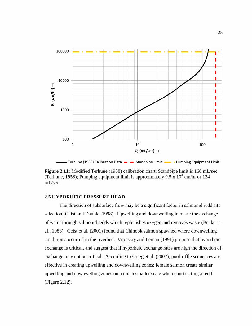
determine hydraulic conductivity (K) values based on a calibration chart (Figure 2.11).

Permeability data are reported in tables that include range, mean, standard deviation, and

the coefficient of variation. The coefficient of variation is explained in Chapter 2.3.

24

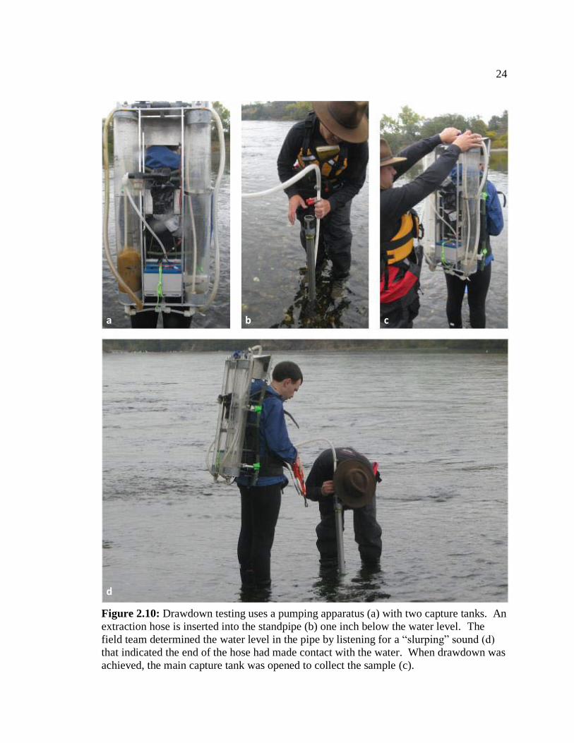
Figure 2.10: Drawdown testing uses a pumping apparatus (a) with two capture tanks. An

extraction hose is inserted into the standpipe (b) one inch below the water level. The

field team determined the water level in the pipe by listening for a “slurping” sound (d)

that indicated the end of the hose had made contact with the water. When drawdown was

achieved, the main capture tank was opened to collect the sample (c).

a b c

d

25

Figure 2.11: Modified Terhune (1958) calibration chart; Standpipe limit is 160 mL/sec

(Terhune, 1958); Pumping equipment limit is approximately 9.5 x 104 cm/hr or 124

mL/sec.

2.5 HYPORHEIC PRESSURE HEAD

The direction of subsurface flow may be a significant factor in salmonid redd site

selection (Geist and Dauble, 1998). Upwelling and downwelling increase the exchange

of water through salmonid redds which replenishes oxygen and removes waste (Becker et

al., 1983). Geist et al. (2001) found that Chinook salmon spawned where downwelling

conditions occurred in the riverbed. Vronskiy and Leman (1991) propose that hyporheic

exchange is critical, and suggest that if hyporheic exchange rates are high the direction of

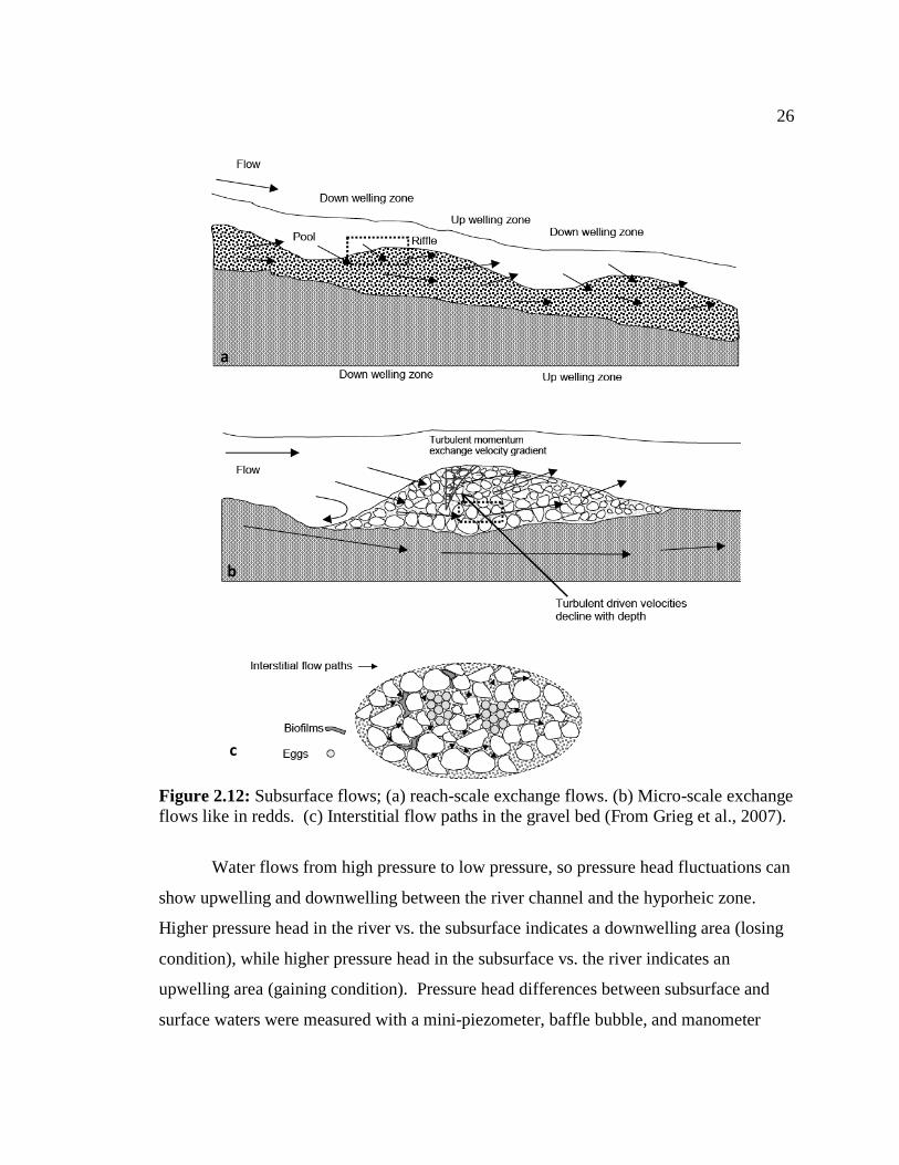
exchange may not be critical. According to Grieg et al. (2007), pool-riffle sequences are

effective in creating upwelling and downwelling zones; female salmon create similar

upwelling and downwelling zones on a much smaller scale when constructing a redd

(Figure 2.12).

100

1000

10000

100000

1 10 100

K (

cm/h

r) →

Q (mL/sec) →

Terhune (1958) Calibration Data Standpipe Limit Pumping Equipment Limit

26

Figure 2.12: Subsurface flows; (a) reach-scale exchange flows. (b) Micro-scale exchange

flows like in redds. (c) Interstitial flow paths in the gravel bed (From Grieg et al., 2007).

Water flows from high pressure to low pressure, so pressure head fluctuations can

show upwelling and downwelling between the river channel and the hyporheic zone.

Higher pressure head in the river vs. the subsurface indicates a downwelling area (losing

condition), while higher pressure head in the subsurface vs. the river indicates an

upwelling area (gaining condition). Pressure head differences between subsurface and

surface waters were measured with a mini-piezometer, baffle bubble, and manometer

a

b

c

27

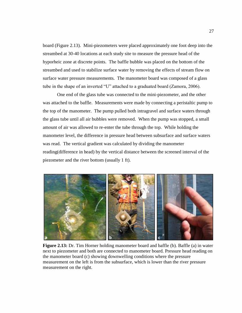
board (Figure 2.13). Mini-piezometers were placed approximately one foot deep into the

streambed at 30-40 locations at each study site to measure the pressure head of the

hyporheic zone at discrete points. The baffle bubble was placed on the bottom of the

streambed and used to stabilize surface water by removing the effects of stream flow on

surface water pressure measurements. The manometer board was composed of a glass

tube in the shape of an inverted “U” attached to a graduated board (Zamora, 2006).

One end of the glass tube was connected to the mini-piezometer, and the other

was attached to the baffle. Measurements were made by connecting a peristaltic pump to

the top of the manometer. The pump pulled both intragravel and surface waters through

the glass tube until all air bubbles were removed. When the pump was stopped, a small

amount of air was allowed to re-enter the tube through the top. While holding the

manometer level, the difference in pressure head between subsurface and surface waters

was read. The vertical gradient was calculated by dividing the manometer

reading(difference in head) by the vertical distance between the screened interval of the

piezometer and the river bottom (usually 1 ft).

Figure 2.13: Dr. Tim Horner holding manometer board and baffle (b). Baffle (a) in water

next to piezometer and both are connected to manometer board. Pressure head reading on

the manometer board (c) showing downwelling conditions where the pressure

measurement on the left is from the subsurface, which is lower than the river pressure

measurement on the right.

c b a

28

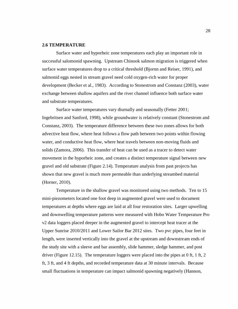
2.6 TEMPERATURE

Surface water and hyporheic zone temperatures each play an important role in

successful salomonid spawning. Upstream Chinook salmon migration is triggered when

surface water temperatures drop to a critical threshold (Bjornn and Reiser, 1991), and

salmonid eggs nested in stream gravel need cold oxygen-rich water for proper

development (Becker et al., 1983). According to Stonestrom and Constanz (2003), water

exchange between shallow aquifers and the river channel influence both surface water

and substrate temperatures.

Surface water temperatures vary diurnally and seasonally (Fetter 2001;

Ingebritsen and Sanford, 1998), while groundwater is relatively constant (Stonestrom and

Constanz, 2003). The temperature difference between these two zones allows for both

advective heat flow, where heat follows a flow path between two points within flowing

water, and conductive heat flow, where heat travels between non-moving fluids and

solids (Zamora, 2006). This transfer of heat can be used as a tracer to detect water

movement in the hyporheic zone, and creates a distinct temperature signal between new

gravel and old substrate (Figure 2.14). Temperature analysis from past projects has

shown that new gravel is much more permeable than underlying streambed material

(Horner, 2010).

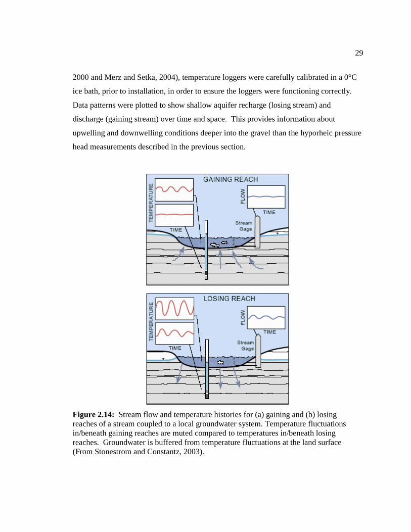
Temperature in the shallow gravel was monitored using two methods. Ten to 15

mini-piezometers located one foot deep in augmented gravel were used to document

temperatures at depths where eggs are laid at all four restoration sites. Larger upwelling

and downwelling temperature patterns were measured with Hobo Water Temperature Pro

v2 data loggers placed deeper in the augmented gravel to intercept heat tracer at the

Upper Sunrise 2010/2011 and Lower Sailor Bar 2012 sites. Two pvc pipes, four feet in

length, were inserted vertically into the gravel at the upstream and downstream ends of

the study site with a sleeve and bar assembly, slide hammer, sledge hammer, and post

driver (Figure 12.15). The temperature loggers were placed into the pipes at 0 ft, 1 ft, 2

ft, 3 ft, and 4 ft depths, and recorded temperature data at 30 minute intervals. Because

small fluctuations in temperature can impact salmonid spawning negatively (Hannon,

29

2000 and Merz and Setka, 2004), temperature loggers were carefully calibrated in a 0°C

ice bath, prior to installation, in order to ensure the loggers were functioning correctly.

Data patterns were plotted to show shallow aquifer recharge (losing stream) and

discharge (gaining stream) over time and space. This provides information about

upwelling and downwelling conditions deeper into the gravel than the hyporheic pressure

head measurements described in the previous section.

Figure 2.14: Stream flow and temperature histories for (a) gaining and (b) losing

reaches of a stream coupled to a local groundwater system. Temperature fluctuations

in/beneath gaining reaches are muted compared to temperatures in/beneath losing

reaches. Groundwater is buffered from temperature fluctuations at the land surface

(From Stonestrom and Constantz, 2003).

30

Figure 2.15: A string of (c) Hobo water Temp Pro v2 data loggers are affixed at (b) 0

foot (gravel river interface), 1 foot, 2 foot, 3 foot, 4 foot intervals and inserted into the

streambed using a (a) sleeve assembly and post driver. Data is retrieved by (d)

connecting each logger to a computer and uploading information.

2.7 HYPORHEIC WATER QUALITY

On the American River, salmonids construct redds approximately one foot deep in

streambed gravels (Hannon, 2000), taking advantage of the groundwater-surface water

interface in the hyporheic zone. Stream water flows through this zone, exchanging

oxygen and transporting dissolved ions through the gravel. Incubating eggs are exposed

to this environment and dependent on intragravel flow of hyporheic water for the delivery

a

b c d

31

of oxygen and the removal of metabolic waste (Youngson et al., 2004; Kondolf, 2008).

Dissolved oxygen, pH, electrical conductivity and turbidity each provide information

about water quality and flow in the hyporheic zone.

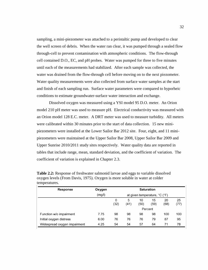
Dissolved oxygen can be a limiting factor in salmonid reproduction. Multiple

factors control oxygen content in the hyporheic environment (Malcolm et al., 2002),

including temperature (Davis, 1975). Low dissolved oxygen content has been linked to

salmonid egg mortality, as well as low overall fitness of eggs and alevin (Nawa et al.,

1990; DeVries, 2000; Malcolm et al. 2003; Youngson et al. 2004; Horner, 2004; Kondolf

et al., 2008). The minimum oxygen necessary for developing salmonid embryos is

between 4 mg/L and 6 mg/L (Table 2.2). Additionally, dissolved oxygen saturation is

inversely correlated with electrical conductivity. Low dissolved oxygen and high

electrical conductivity levels are representative of groundwater with long residence times

and low intragravel flow. Mineral ion dissolution results in a rise in electrical

conductivity, while low dissolved oxygen content may produce reducing conditions

(Figure 2.16) and result in anaerobic bacterial activity in the hyporheic zone (Youngson

et al., 2004).

A high percent of suspended sediment or turbidity can be an indicator of an

impaired stream habitat, and fine sediment intrusion and accumulation in riverbed gravels

can significantly reduce permeability (Wu, 2000; Soulsby et al., 2001; Bash et al., 2001).

The Environmental Protection Agency (EPA) has identified siltation as the most

important source of water quality degradation on rivers. From a biological standpoint,

the density and diversity of macro-invertebrates can be impacted by turbidity, thereby

negatively affecting the food web at higher trophic levels and older salmonid life stages

such as fry and adult salmon (Henley et al., 2000, Bash et al., 2001).

At each restoration site, subsurface water quality parameters were measured to

characterize the chemical conditions experienced by incubating eggs. Ten to 15 mini-

piezometers were installed one foot deep into the gravel at each study site and sampled

for dissolved oxygen (D.O.), turbidity, electrical conductivity (EC), pH, and temperature.

Mini-piezometers were sampled seasonally at each location (Figure 2.17). During

32

sampling, a mini-piezometer was attached to a peristaltic pump and developed to clear

the well screen of debris. When the water ran clear, it was pumped through a sealed flow

through-cell to prevent contamination with atmospheric conditions. The flow-through

cell contained D.O., EC, and pH probes. Water was pumped for three to five minutes

until each of the measurements had stabilized. After each sample was collected, the

water was drained from the flow-through cell before moving on to the next piezometer.

Water quality measurements were also collected from surface water samples at the start

and finish of each sampling run. Surface water parameters were compared to hyporheic

conditions to estimate groundwater-surface water interaction and exchange.

Dissolved oxygen was measured using a YSI model 95 D.O. meter. An Orion

model 210 pH meter was used to measure pH. Electrical conductivity was measured with

an Orion model 128 E.C. meter. A DRT meter was used to measure turbidity. All meters

were calibrated within 30 minutes prior to the start of data collection. 15 new mini-

piezometers were installed at the Lower Sailor Bar 2012 site. Four, eight, and 11 mini-

piezometers were maintained at the Upper Sailor Bar 2008, Upper Sailor Bar 2009 and

Upper Sunrise 2010/2011 study sites respectively. Water quality data are reported in

tables that include range, mean, standard deviation, and the coefficient of variation. The

coefficient of variation is explained in Chapter 2.3.

Table 2.2: Response of freshwater salmonid larvae and eggs to variable dissolved

oxygen levels (From Davis, 1975). Oxygen is more soluble in water at colder

temperatures.

33

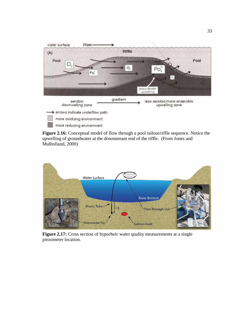
Figure 2.16: Conceptual model of flow through a pool tailout/riffle sequence. Notice the

upwelling of groundwater at the downstream end of the riffle. (From Jones and

Mulholland, 2000)

Figure 2.17: Cross section of hyporheic water quality measurements at a single

piezometer location.

34

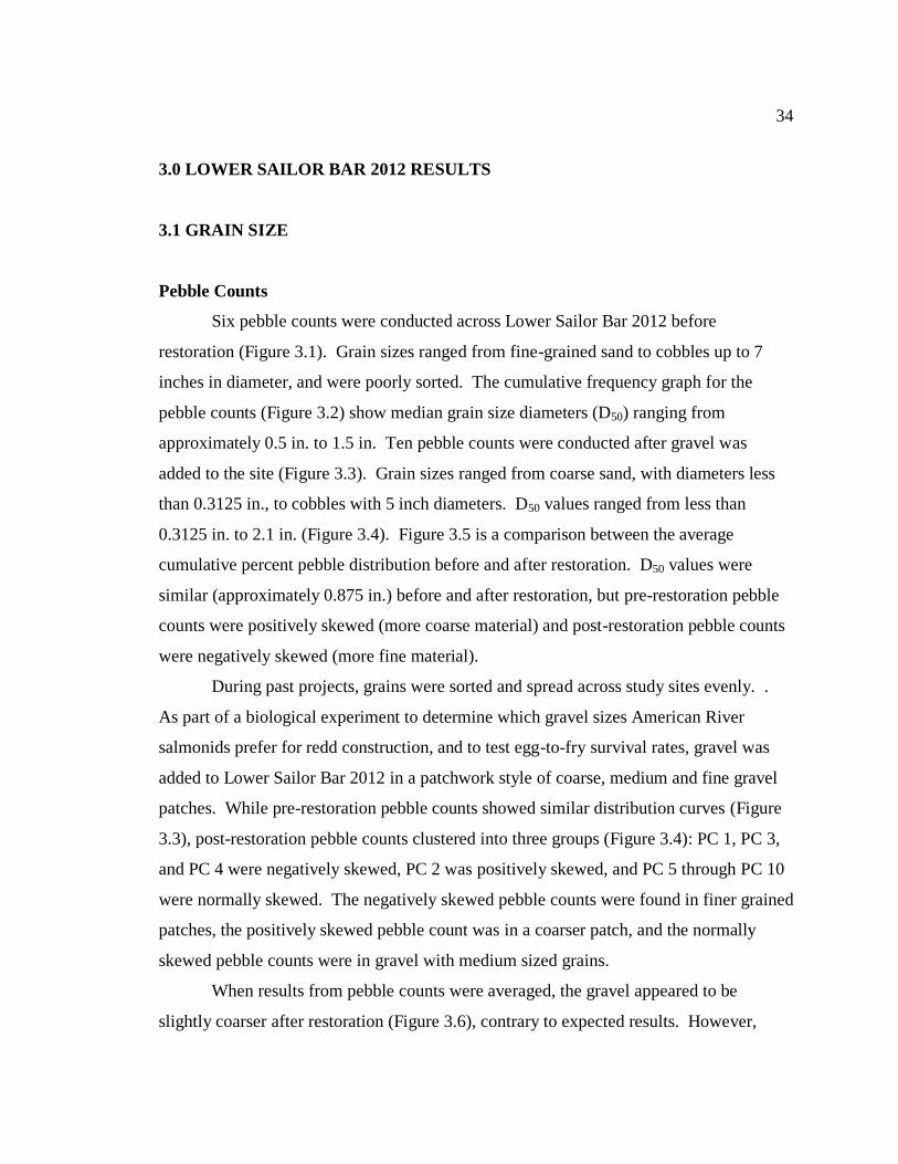
3.0 LOWER SAILOR BAR 2012 RESULTS

3.1 GRAIN SIZE

Pebble Counts

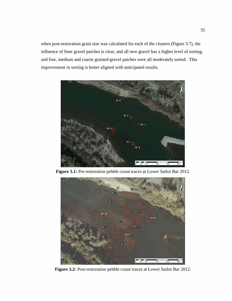
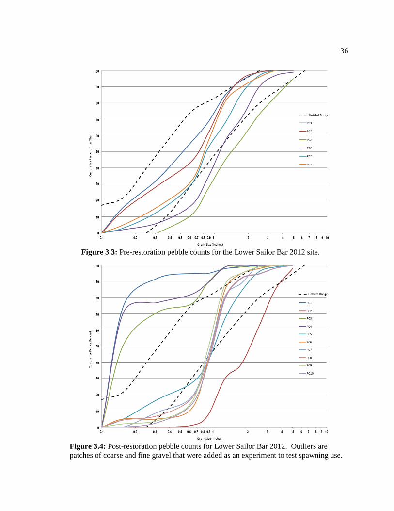
Six pebble counts were conducted across Lower Sailor Bar 2012 before

restoration (Figure 3.1). Grain sizes ranged from fine-grained sand to cobbles up to 7

inches in diameter, and were poorly sorted. The cumulative frequency graph for the

pebble counts (Figure 3.2) show median grain size diameters (D50) ranging from

approximately 0.5 in. to 1.5 in. Ten pebble counts were conducted after gravel was

added to the site (Figure 3.3). Grain sizes ranged from coarse sand, with diameters less

than 0.3125 in., to cobbles with 5 inch diameters. D50 values ranged from less than

0.3125 in. to 2.1 in. (Figure 3.4). Figure 3.5 is a comparison between the average

cumulative percent pebble distribution before and after restoration. D50 values were

similar (approximately 0.875 in.) before and after restoration, but pre-restoration pebble

counts were positively skewed (more coarse material) and post-restoration pebble counts

were negatively skewed (more fine material).

During past projects, grains were sorted and spread across study sites evenly. .

As part of a biological experiment to determine which gravel sizes American River

salmonids prefer for redd construction, and to test egg-to-fry survival rates, gravel was

added to Lower Sailor Bar 2012 in a patchwork style of coarse, medium and fine gravel

patches. While pre-restoration pebble counts showed similar distribution curves (Figure

3.3), post-restoration pebble counts clustered into three groups (Figure 3.4): PC 1, PC 3,

and PC 4 were negatively skewed, PC 2 was positively skewed, and PC 5 through PC 10

were normally skewed. The negatively skewed pebble counts were found in finer grained

patches, the positively skewed pebble count was in a coarser patch, and the normally

skewed pebble counts were in gravel with medium sized grains.

When results from pebble counts were averaged, the gravel appeared to be

slightly coarser after restoration (Figure 3.6), contrary to expected results. However,

35

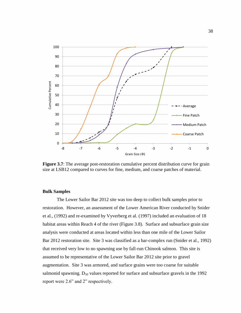
when post-restoration grain size was calculated for each of the clusters (Figure 3.7), the

influence of finer gravel patches is clear, and all new gravel has a higher level of sorting,

and fine, medium and coarse grained-gravel patches were all moderately sorted. This

improvement in sorting is better aligned with anticipated results.

Figure 3.1: Pre-restoration pebble count traces at Lower Sailor Bar 2012.

Figure 3.2: Post-restoration pebble count traces at Lower Sailor Bar 2012.

36

Figure 3.3: Pre-restoration pebble counts for the Lower Sailor Bar 2012 site.

Figure 3.4: Post-restoration pebble counts for Lower Sailor Bar 2012. Outliers are

patches of coarse and fine gravel that were added as an experiment to test spawning use.

37

Figure 3.5: Lower Sailor Bar 2012 average pebble frequency before and after restoration.

Figure 3.6: Pebble count averages at Lower Sailor Bar 2012 before and after restoration.

0

10

20

30

40

50

60

70

80

90

100

-8 -7 -6 -5 -4 -3 -2 -1 0

Cu

mu

lati

ve P

erce

nt

Grain Size (Φ)

LSB Pre-Restoration

LSB12 Post-Restoration

38

Figure 3.7: The average post-restoration cumulative percent distribution curve for grain

size at LSB12 compared to curves for fine, medium, and coarse patches of material.

Bulk Samples

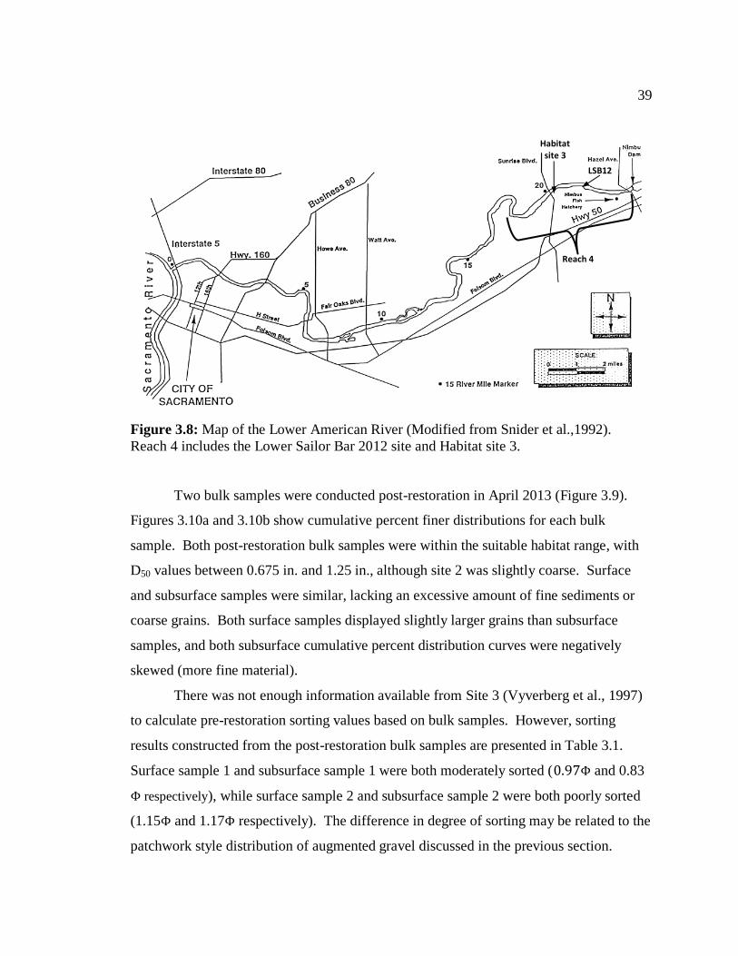
The Lower Sailor Bar 2012 site was too deep to collect bulk samples prior to

restoration. However, an assessment of the Lower American River conducted by Snider

et al., (1992) and re-examined by Vyverberg et al. (1997) included an evaluation of 18

habitat areas within Reach 4 of the river (Figure 3.8). Surface and subsurface grain size

analysis were conducted at areas located within less than one mile of the Lower Sailor

Bar 2012 restoration site. Site 3 was classified as a bar-complex run (Snider et al., 1992)

that received very low to no spawning use by fall-run Chinook salmon. This site is

assumed to be representative of the Lower Sailor Bar 2012 site prior to gravel

augmentation. Site 3 was armored, and surface grains were too coarse for suitable

salmonid spawning. D50 values reported for surface and subsurface gravels in the 1992

report were 2.6” and 2” respectively.

0

10

20

30

40

50

60

70

80

90

100

-8 -7 -6 -5 -4 -3 -2 -1 0

Cu

mu

lati

ve P

erce

nt

Grain Size (Φ)

Average

Fine Patch

Medium Patch

Coarse Patch

39

Figure 3.8: Map of the Lower American River (Modified from Snider et al.,1992).

Reach 4 includes the Lower Sailor Bar 2012 site and Habitat site 3.

Two bulk samples were conducted post-restoration in April 2013 (Figure 3.9).

Figures 3.10a and 3.10b show cumulative percent finer distributions for each bulk

sample. Both post-restoration bulk samples were within the suitable habitat range, with

D50 values between 0.675 in. and 1.25 in., although site 2 was slightly coarse. Surface

and subsurface samples were similar, lacking an excessive amount of fine sediments or

coarse grains. Both surface samples displayed slightly larger grains than subsurface

samples, and both subsurface cumulative percent distribution curves were negatively

skewed (more fine material).

There was not enough information available from Site 3 (Vyverberg et al., 1997)

to calculate pre-restoration sorting values based on bulk samples. However, sorting

results constructed from the post-restoration bulk samples are presented in Table 3.1.

Surface sample 1 and subsurface sample 1 were both moderately sorted ( and 0.83

respectively), while surface sample 2 and subsurface sample 2 were both poorly sorted

(1.15 and 1.17 respectively). The difference in degree of sorting may be related to the

patchwork style distribution of augmented gravel discussed in the previous section.

Reach 4

LSB12

Habitat site 3

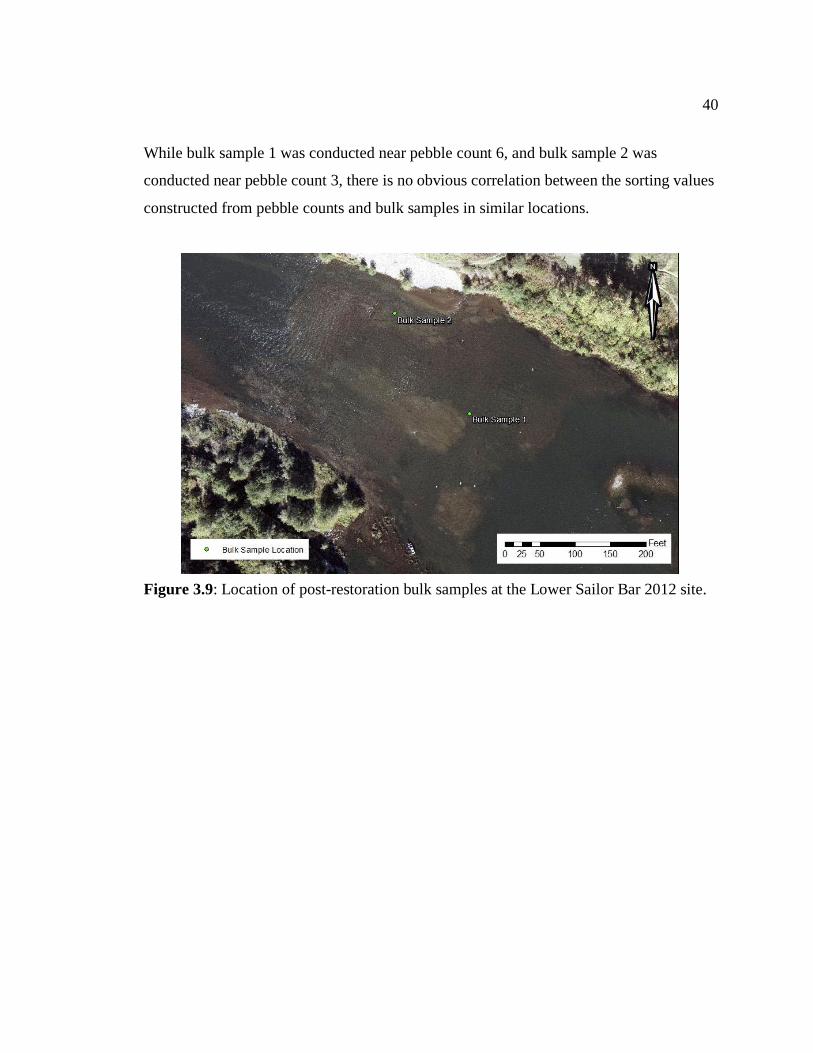
40

While bulk sample 1 was conducted near pebble count 6, and bulk sample 2 was

conducted near pebble count 3, there is no obvious correlation between the sorting values

constructed from pebble counts and bulk samples in similar locations.

Figure 3.9: Location of post-restoration bulk samples at the Lower Sailor Bar 2012 site.

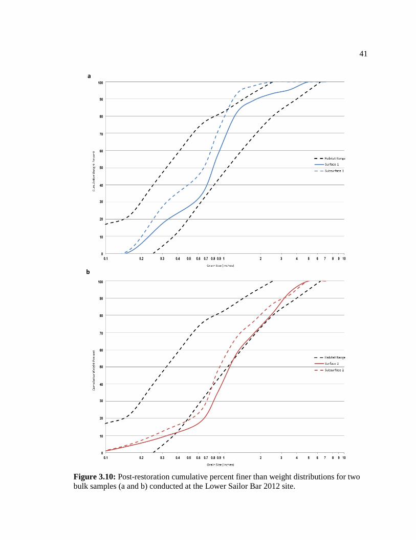
41

Figure 3.10: Post-restoration cumulative percent finer than weight distributions for two

bulk samples (a and b) conducted at the Lower Sailor Bar 2012 site.

a

b

42

Table 3.1: Sorting results for post-restoration bulk samples at the Lower Sailor Bar 2012

site collected in April 2013.

Surface Sample 1 Subsurface Sample 1 Surface Sample 2 Subsurface Sample 2

D84 -3.8 -3.5 -4.35 -4.55

D16 -5.59 -5.25 -6.58 -6.8

D95 -3.2 -3.1 -3.15 -3.6

D5 -6.71 -5.69 -7.05 -7.6

σi 0.97 0.83 1.15 1.17

Sorting Moderately sorted Moderately sorted Poorly sorted Poorly sorted

3.2 GRAVEL MOBILITY

Tracer Rocks

Figure 3.11: Post gravel addition map of Lower Sailor Bar 2012 showing initial

placement of tracer rocks. Large (2.5 in. - 3 in.), medium (1.25 in. - 1.75 in.), and small

(0.625 in. - 0.875 in.) tracer rocks were placed at each point on the map.

Tracer rocks were deployed at the study site following gravel augmentation in

September 2012. Small groupings of tracer rocks (small, medium, large) were placed at

43

discrete points along one of three transects across the study site (upstream, middle,

downstream) as shown in Figure 3.11. Tracer rocks were relocated in April 2013

following the winter season. River flows between October 2012 and April 2013 ranged

from a low of 942 cfs to a high of 9,980 cfs with a mean flow of 2,382 cfs. Flows above

5,000 cfs persisted throughout the month of December. As of April 16, 2013, tracer

rocks showed little to no movement.

Scour Chains

Figure 3.12: Scour and fill map of the Lower Sailor Bar 2012 site.

Following gravel augmentation in September 2012, 15 scour chains were installed

at the Lower Sailor Bar 2012 study site (Figure 3.12). As of April 2013, eight of the

original chains were recovered. The missing chains were primarily at the downstream

end of the site, and may have been buried as gravel was eroded from the head of the riffle

and redeposited in downstream locations. The remaining chains all displayed an increase

in chain length indicating scour across the site. The greatest amount of scour (5.12 in.)

Upstream

Downstream

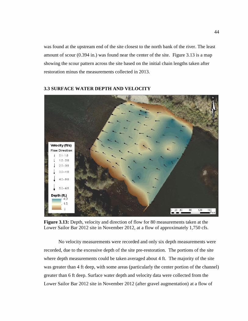
44

was found at the upstream end of the site closest to the north bank of the river. The least

amount of scour (0.394 in.) was found near the center of the site. Figure 3.13 is a map

showing the scour pattern across the site based on the initial chain lengths taken after

restoration minus the measurements collected in 2013.


Figure 3.13: Depth, velocity and direction of flow for 80 measurements taken at the

Lower Sailor Bar 2012 site in November 2012, at a flow of approximately 1,750 cfs.

No velocity measurements were recorded and only six depth measurements were

recorded, due to the excessive depth of the site pre-restoration. The portions of the site

where depth measurements could be taken averaged about 4 ft. The majority of the site

was greater than 4 ft deep, with some areas (particularly the center portion of the channel)

greater than 6 ft deep. Surface water depth and velocity data were collected from the

Lower Sailor Bar 2012 site in November 2012 (after gravel augmentation) at a flow of

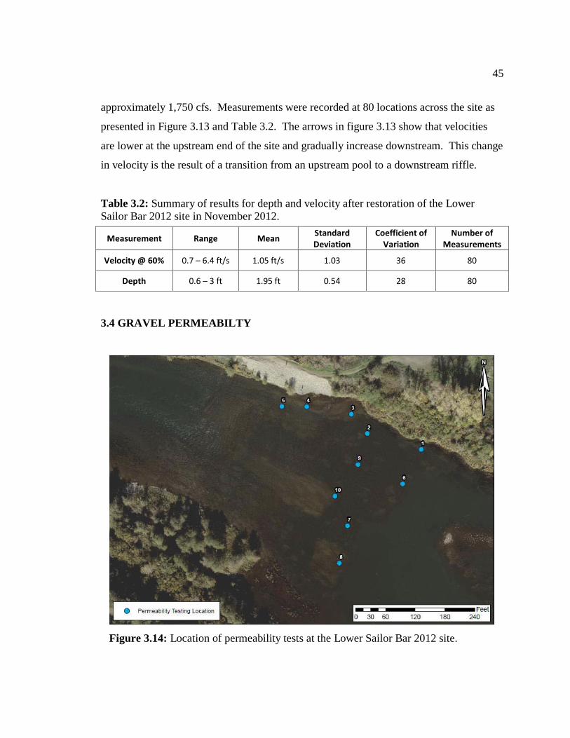
45

approximately 1,750 cfs. Measurements were recorded at 80 locations across the site as

presented in Figure 3.13 and Table 3.2. The arrows in figure 3.13 show that velocities

are lower at the upstream end of the site and gradually increase downstream. This change

in velocity is the result of a transition from an upstream pool to a downstream riffle.

Table 3.2: Summary of results for depth and velocity after restoration of the Lower

Sailor Bar 2012 site in November 2012.

Measurement Range Mean Standard Deviation

Coefficient of Variation

Number of Measurements

Velocity @ 60% 0.7 – 6.4 ft/s 1.05 ft/s 1.03 36 80

Depth 0.6 – 3 ft 1.95 ft 0.54 28 80

3.4 GRAVEL PERMEABILTY

Figure 3.14: Location of permeability tests at the Lower Sailor Bar 2012 site.

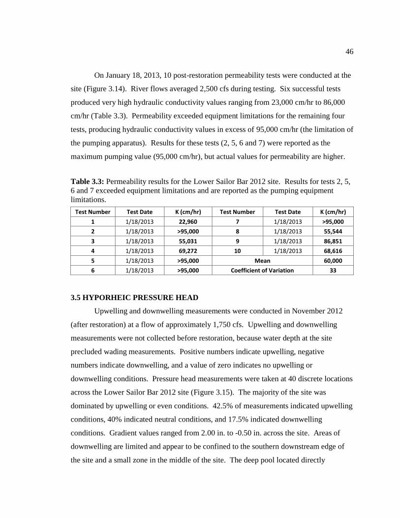
46

On January 18, 2013, 10 post-restoration permeability tests were conducted at the

site (Figure 3.14). River flows averaged 2,500 cfs during testing. Six successful tests

produced very high hydraulic conductivity values ranging from 23,000 cm/hr to 86,000

cm/hr (Table 3.3). Permeability exceeded equipment limitations for the remaining four

tests, producing hydraulic conductivity values in excess of 95,000 cm/hr (the limitation of

the pumping apparatus). Results for these tests (2, 5, 6 and 7) were reported as the

maximum pumping value (95,000 cm/hr), but actual values for permeability are higher.

Table 3.3: Permeability results for the Lower Sailor Bar 2012 site. Results for tests 2, 5,

6 and 7 exceeded equipment limitations and are reported as the pumping equipment

limitations.

Test Number Test Date K (cm/hr) Test Number Test Date K (cm/hr)

1 1/18/2013 22,960 7 1/18/2013 >95,000

2 1/18/2013 >95,000 8 1/18/2013 55,544

3 1/18/2013 55,031 9 1/18/2013 86,851

4 1/18/2013 69,272 10 1/18/2013 68,616

5 1/18/2013 >95,000 Mean 60,000

6 1/18/2013 >95,000 Coefficient of Variation 33


Upwelling and downwelling measurements were conducted in November 2012

(after restoration) at a flow of approximately 1,750 cfs. Upwelling and downwelling

measurements were not collected before restoration, because water depth at the site

precluded wading measurements. Positive numbers indicate upwelling, negative

numbers indicate downwelling, and a value of zero indicates no upwelling or

downwelling conditions. Pressure head measurements were taken at 40 discrete locations

across the Lower Sailor Bar 2012 site (Figure 3.15). The majority of the site was

dominated by upwelling or even conditions. 42.5% of measurements indicated upwelling

conditions, 40% indicated neutral conditions, and 17.5% indicated downwelling

conditions. Gradient values ranged from 2.00 in. to -0.50 in. across the site. Areas of

downwelling are limited and appear to be confined to the southern downstream edge of

the site and a small zone in the middle of the site. The deep pool located directly

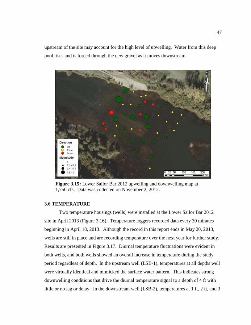
47

upstream of the site may account for the high level of upwelling. Water from this deep

pool rises and is forced through the new gravel as it moves downstream.

Figure 3.15: Lower Sailor Bar 2012 upwelling and downwelling map at

1,750 cfs. Data was collected on November 2, 2012.

3.6 TEMPERATURE

Two temperature housings (wells) were installed at the Lower Sailor Bar 2012

site in April 2013 (Figure 3.16). Temperature loggers recorded data every 30 minutes

beginning in April 18, 2013. Although the record in this report ends in May 20, 2013,

wells are still in place and are recording temperature over the next year for further study.

Results are presented in Figure 3.17. Diurnal temperature fluctuations were evident in

both wells, and both wells showed an overall increase in temperature during the study

period regardless of depth. In the upstream well (LSB-1), temperatures at all depths well

were virtually identical and mimicked the surface water pattern. This indicates strong

downwelling conditions that drive the diurnal temperature signal to a depth of 4 ft with

little or no lag or delay. In the downstream well (LSB-2), temperatures at 1 ft, 2 ft, and 3

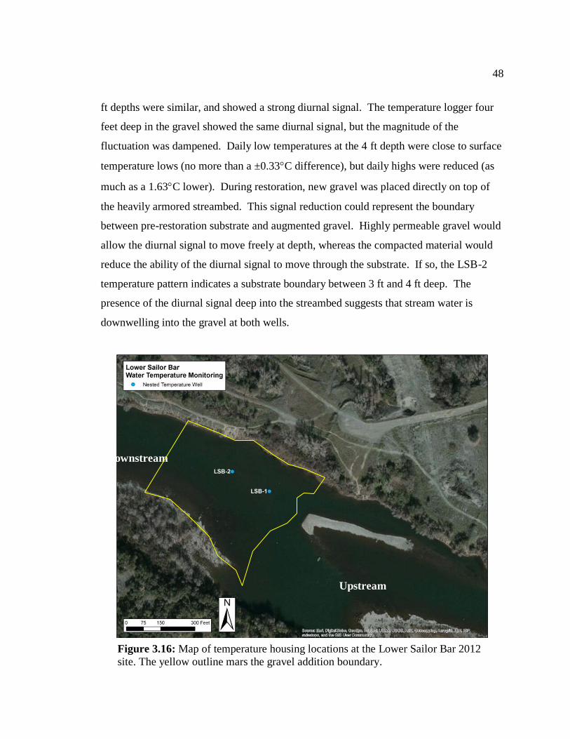
48

ft depths were similar, and showed a strong diurnal signal. The temperature logger four

feet deep in the gravel showed the same diurnal signal, but the magnitude of the

fluctuation was dampened. Daily low temperatures at the 4 ft depth were close to surface

temperature lows (no more than a ±0.33C difference), but daily highs were reduced (as

much as a 1.63C lower). During restoration, new gravel was placed directly on top of

the heavily armored streambed. This signal reduction could represent the boundary

between pre-restoration substrate and augmented gravel. Highly permeable gravel would

allow the diurnal signal to move freely at depth, whereas the compacted material would

reduce the ability of the diurnal signal to move through the substrate. If so, the LSB-2

temperature pattern indicates a substrate boundary between 3 ft and 4 ft deep. The

presence of the diurnal signal deep into the streambed suggests that stream water is

downwelling into the gravel at both wells.

Figure 3.16: Map of temperature housing locations at the Lower Sailor Bar 2012

site. The yellow outline mars the gravel addition boundary.

Upstream

Downstream

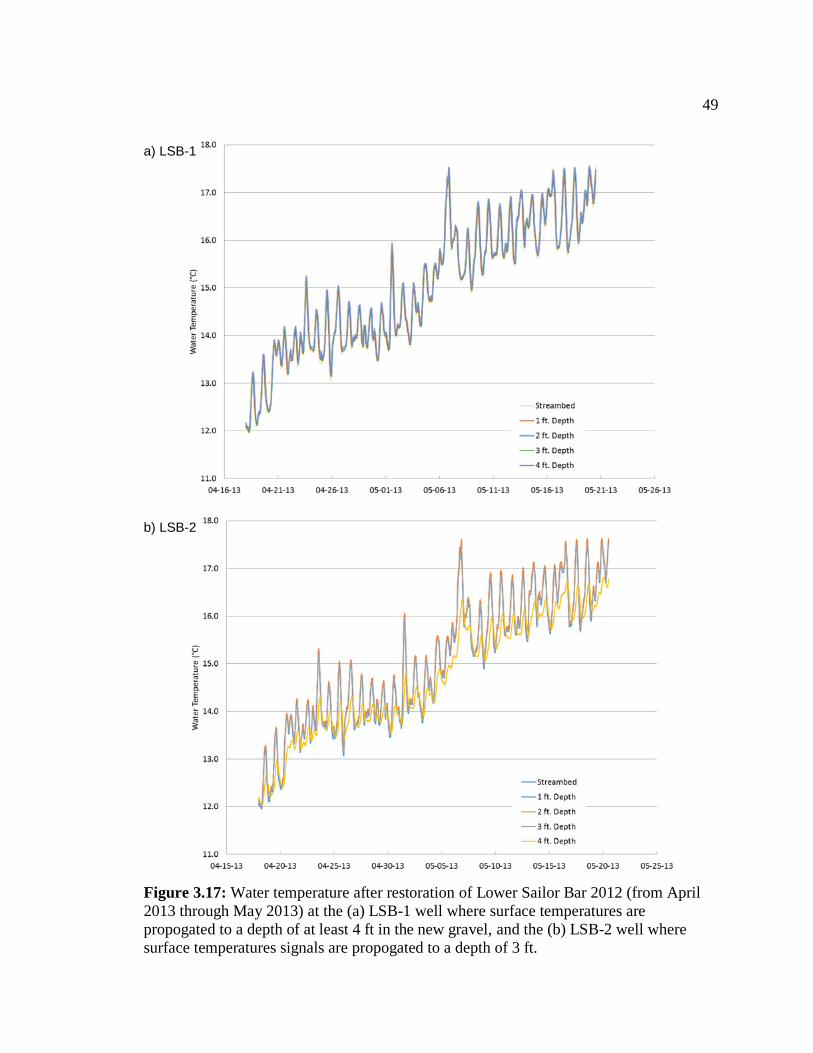
49

a) LSB-1

b) LSB-2

Figure 3.17: Water temperature after restoration of Lower Sailor Bar 2012 (from April

2013 through May 2013) at the (a) LSB-1 well where surface temperatures are

propogated to a depth of at least 4 ft in the new gravel, and the (b) LSB-2 well where

surface temperatures signals are propogated to a depth of 3 ft.

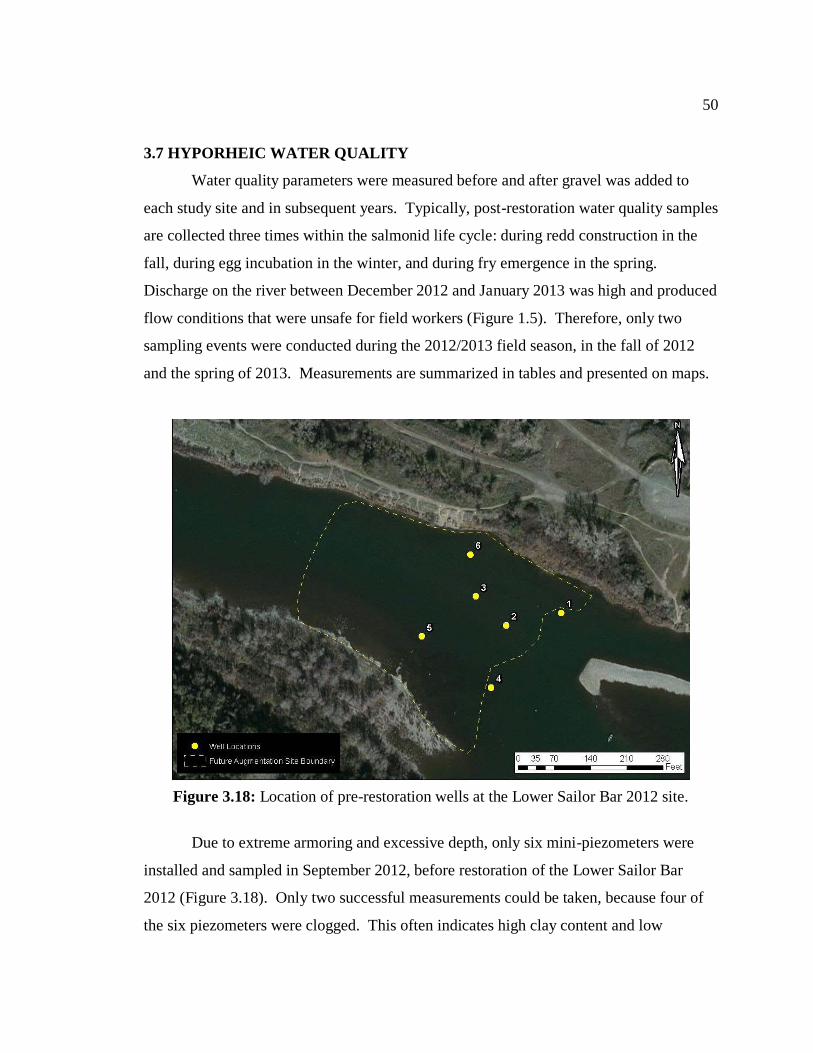
50


Water quality parameters were measured before and after gravel was added to

each study site and in subsequent years. Typically, post-restoration water quality samples

are collected three times within the salmonid life cycle: during redd construction in the

fall, during egg incubation in the winter, and during fry emergence in the spring.

Discharge on the river between December 2012 and January 2013 was high and produced

flow conditions that were unsafe for field workers (Figure 1.5). Therefore, only two

sampling events were conducted during the 2012/2013 field season, in the fall of 2012

and the spring of 2013. Measurements are summarized in tables and presented on maps.

Figure 3.18: Location of pre-restoration wells at the Lower Sailor Bar 2012 site.

Due to extreme armoring and excessive depth, only six mini-piezometers were

installed and sampled in September 2012, before restoration of the Lower Sailor Bar

2012 (Figure 3.18). Only two successful measurements could be taken, because four of

the six piezometers were clogged. This often indicates high clay content and low

51

permeability. Table 3.4 shows pre-restoration water quality data. The dissolved oxygen

(D.O.) levels ranged from 2.53 mg/L to 3.26 mg/L, and D.O. saturation ranged from 36%

to 40%.

Table 3.4: Lower Sailor Bar 2012 Pre-Restoration Water Quality Parameters

Location D.O. (mg/L) D.O. (% sat) E.C. (uS) pH Turbidity (NTU)

2 2.53 40 56.8 6.54 8.5

3 3.26 36 59.5 6.61 26.8

Surface 1 9 69 47.1 6.77 18

Surface 2 9.14 99.2 47.2 678 18.6

Parameters were collected in September 2012 at approximately 1,750 cfs with an average

hyporheic temperature of 18.5C. Piezometers at locations 1, 4, 5 and 6 were clogged.

Figure 3.19: Location map of mini-piezometers after restoration.

After restoration, 15 mini-piezometers were installed at the site (Figure 3.19) and

sampled in November 2012 and April 2013. Tables 3.5 and 3.6 show post-restoration

Fall and Spring water quality data respectively. In November, 13 samples were collected

52

successfully. The mean D.O. level during redd construction was 9.52 mg/L with values

ranging from 8.95 mg/L to 9.98 mg/L, and the mean D.O. saturation was 93.7% with

values ranging from 88.1% to 97.8%. In April, water quality measurements were

collected from 11 locations. The mean D.O. level decreased during fry emergence to

7.94 mg/L with values ranging from 7.02 mg/L to 8.25 mg/L, and the mean D.O.

saturation dropped to 77.2% with values ranging from 69% to 83%. The well at location

8 showed the greatest difference in D.O. levels between the fall and spring sampling

events (9.67 mg/L and 7.33 mg/L respectively).

Table 3.5: Lower Sailor Bar 2012 Water Quality Parameters as of November 2012


1 9.62 94.2 48.2 7.14 17

2 9.38 93.4 47.9 7.05 4.5

3 9.69 96.8 47.7 7.12 16

4 9.47 94.5 47.5 7.06 3.9

5 9.61 93.6 47.3 7.04 1.6

7 9.76 96.2 47.5 7.23 10

8 9.61 95.9 47.2 7.14 10

9 9.38 92 47.5 7.14 30

10 9.98 97.8 47.8 7.13 42

11 9.04 88.8 48.1 7.24 18

12 9.3 88.1 47.9 7.19 17

13 8.95 90.7 47.4 7.26 3

15 9.98 96 47.3 7.09 50

Mean 9.52 93.69 47.64 7.14 17.15

Coefficient of

Variation 3 3 1 1 88

Surface 1 9.24 91.6 50.8 7.23 4

Surface 2 9.8 97.4 47.4 7.04 1.4

Data were collected in November 2012 (after restoration) at 1,430 cfs. Mean hyporheic

temperature was 15C. Piezometers 6 and 14 were clogged.

Figures 3.20 and 3.21 show Fall and Spring D.O. saturation levels on the Lower

Sailor Bar 2012 Map. Green dots represent high D.O. percentages that are within 90% of

surface water levels and may indicate good intragravel flow. Yellow dots represent D.O.

percentages that are within 60%-90% of surface water measurements. These sites are

reasonable for egg development and survival, but may indicate lower intragravel flow.

53

Red dots represent D.O. percentages that are critically low for egg development and

survival. During Fall sampling, the majority of wells showed high D.O. values and high

saturation. During Spring sampling, all wells showed lower D.O. levels and moderate

saturation.

Table 3.6: Lower Sailor Bar 2012 Water Quality Parameters as of April 2013


1 8.4 83 53 7.2 12

2 8.12 78 54 7.2 6

3 8.25 80 54 7.3 68.5

4 8.01 77 53 7.3 15

5 7.75 75 53 7.2 1.5

7 8.24 80.8 54 7.3 6.5

8 7.33 73 54 7.3 9.5

9 8.03 77 54 7.3 66

10 8.06 78 54 7.3 54

12 8.09 78 54 7.1 20

14 7.02 69 54 7.1 80

Mean 7.94 77.16 53.73 7.24 30.82

Coefficient of


Surface 10 99 53 7.3 1.5

Data were collected in April 2013 at 1,300 cfs. Mean hyporheic temperature was 13.8C.

Piezometer 6 was clogged, and piezometers 11, 13, and 15 were missing.

Figures 3.22 and 3.23 illustrate turbidity levels across the study site during Fall

and Spring sampling events. Darker colors represent higher turbidity values and lighter

colors represent lower values. Pre-restoration and fall post-restoration mean turbidity

values were similar at 17.65 NTU and 17.15 NTU respectively. When compared to the

Fall sampling event, mean turbidity from Spring sampling increased by over 40% from

17.13 NTU to 30.82 NTU. Turbidity in most of the wells increased between the Fall and

Spring sampling events, but well location 3 had the largest increase from 16 NTU to 68.5

NTU.

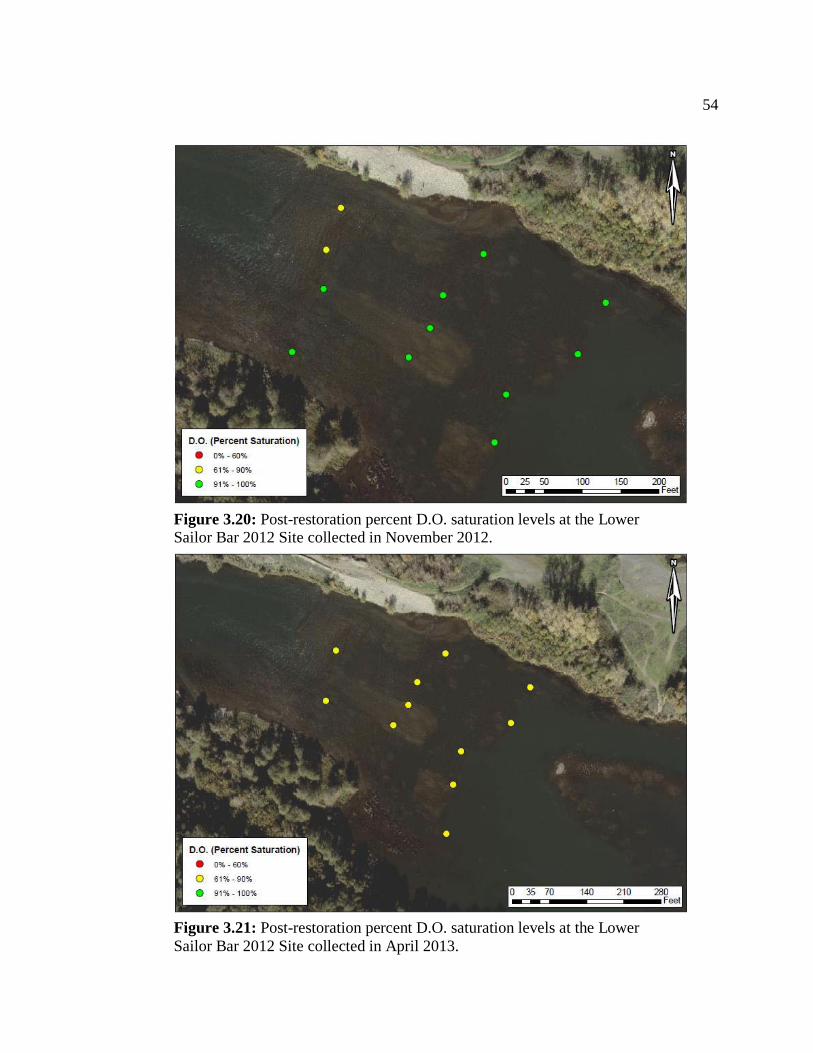
54

Figure 3.20: Post-restoration percent D.O. saturation levels at the Lower Sailor Bar 2012 Site collected in November 2012.

Figure 3.21: Post-restoration percent D.O. saturation levels at the Lower

Sailor Bar 2012 Site collected in April 2013.

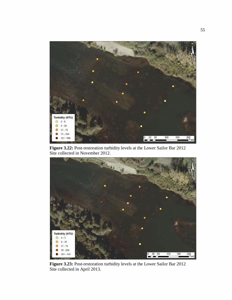
55

Figure 3.22: Post-restoration turbidity levels at the Lower Sailor Bar 2012 Site collected in November 2012.

Figure 3.23: Post-restoration turbidity levels at the Lower Sailor Bar 2012

Site collected in April 2013.

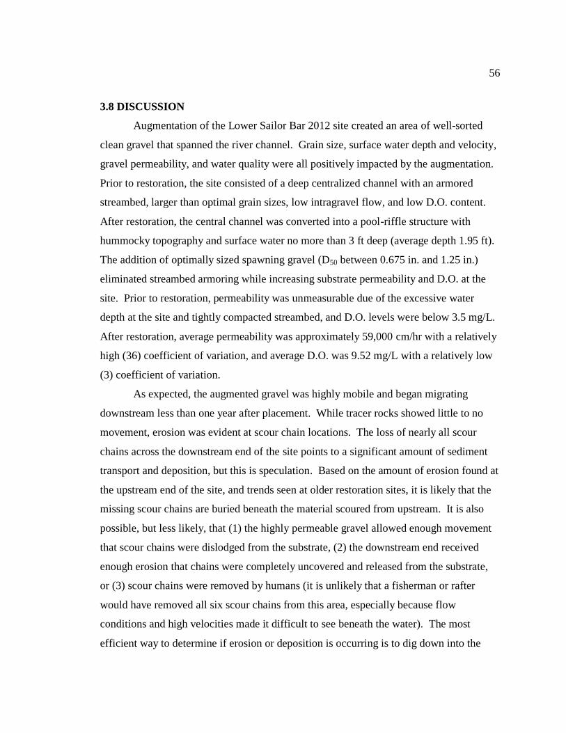
56

3.8 DISCUSSION

Augmentation of the Lower Sailor Bar 2012 site created an area of well-sorted

clean gravel that spanned the river channel. Grain size, surface water depth and velocity,

gravel permeability, and water quality were all positively impacted by the augmentation.

Prior to restoration, the site consisted of a deep centralized channel with an armored

streambed, larger than optimal grain sizes, low intragravel flow, and low D.O. content.

After restoration, the central channel was converted into a pool-riffle structure with

hummocky topography and surface water no more than 3 ft deep (average depth 1.95 ft).

The addition of optimally sized spawning gravel (D50 between 0.675 in. and 1.25 in.)

eliminated streambed armoring while increasing substrate permeability and D.O. at the

site. Prior to restoration, permeability was unmeasurable due of the excessive water

depth at the site and tightly compacted streambed, and D.O. levels were below 3.5 mg/L.

After restoration, average permeability was approximately 59,000 cm/hr with a relatively

high (36) coefficient of variation, and average D.O. was 9.52 mg/L with a relatively low

(3) coefficient of variation.

As expected, the augmented gravel was highly mobile and began migrating

downstream less than one year after placement. While tracer rocks showed little to no

movement, erosion was evident at scour chain locations. The loss of nearly all scour

chains across the downstream end of the site points to a significant amount of sediment

transport and deposition, but this is speculation. Based on the amount of erosion found at

the upstream end of the site, and trends seen at older restoration sites, it is likely that the

missing scour chains are buried beneath the material scoured from upstream. It is also

possible, but less likely, that (1) the highly permeable gravel allowed enough movement

that scour chains were dislodged from the substrate, (2) the downstream end received

enough erosion that chains were completely uncovered and released from the substrate,

or (3) scour chains were removed by humans (it is unlikely that a fisherman or rafter

would have removed all six scour chains from this area, especially because flow

conditions and high velocities made it difficult to see beneath the water). The most

efficient way to determine if erosion or deposition is occurring is to dig down into the

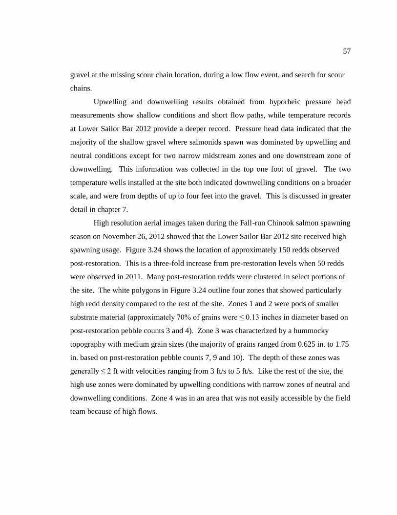
57

gravel at the missing scour chain location, during a low flow event, and search for scour

chains.

Upwelling and downwelling results obtained from hyporheic pressure head

measurements show shallow conditions and short flow paths, while temperature records

at Lower Sailor Bar 2012 provide a deeper record. Pressure head data indicated that the

majority of the shallow gravel where salmonids spawn was dominated by upwelling and

neutral conditions except for two narrow midstream zones and one downstream zone of

downwelling. This information was collected in the top one foot of gravel. The two

temperature wells installed at the site both indicated downwelling conditions on a broader

scale, and were from depths of up to four feet into the gravel. This is discussed in greater

detail in chapter 7.

High resolution aerial images taken during the Fall-run Chinook salmon spawning

season on November 26, 2012 showed that the Lower Sailor Bar 2012 site received high

spawning usage. Figure 3.24 shows the location of approximately 150 redds observed

post-restoration. This is a three-fold increase from pre-restoration levels when 50 redds

were observed in 2011. Many post-restoration redds were clustered in select portions of

the site. The white polygons in Figure 3.24 outline four zones that showed particularly

high redd density compared to the rest of the site. Zones 1 and 2 were pods of smaller

substrate material (approximately 70% of grains were ≤ 0.13 inches in diameter based on

post-restoration pebble counts 3 and 4). Zone 3 was characterized by a hummocky

topography with medium grain sizes (the majority of grains ranged from 0.625 in. to 1.75

in. based on post-restoration pebble counts 7, 9 and 10). The depth of these zones was

generally ≤ 2 ft with velocities ranging from 3 ft/s to 5 ft/s. Like the rest of the site, the

high use zones were dominated by upwelling conditions with narrow zones of neutral and

downwelling conditions. Zone 4 was in an area that was not easily accessible by the field

team because of high flows.

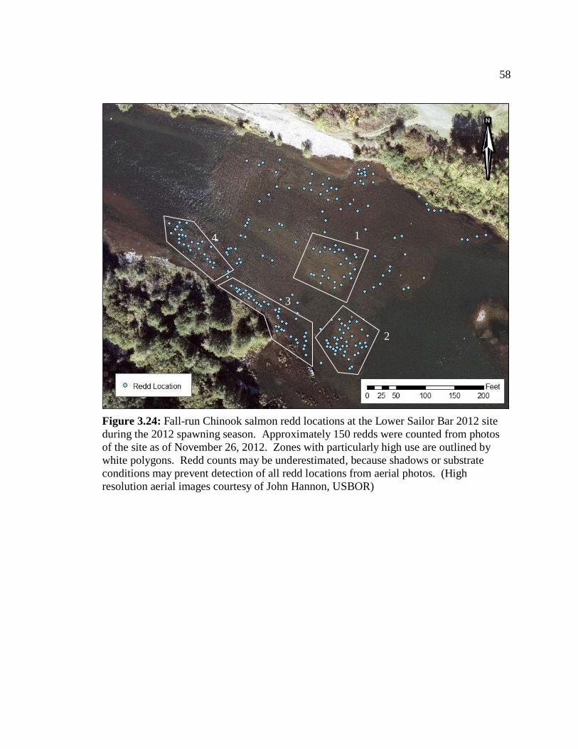
58

Figure 3.24: Fall-run Chinook salmon redd locations at the Lower Sailor Bar 2012 site

during the 2012 spawning season. Approximately 150 redds were counted from photos

of the site as of November 26, 2012. Zones with particularly high use are outlined by

white polygons. Redd counts may be underestimated, because shadows or substrate

conditions may prevent detection of all redd locations from aerial photos. (High

resolution aerial images courtesy of John Hannon, USBOR)

1

2

3

4

59

4.0 UPPER SUNRISE 2010/2011 RESULTS

4.1 GRAVEL MOBILITY

Tracer Rocks

Tracer rocks were deployed at the study site immediately following gravel

augmentation in 2011 and positions tracked in 2012 and 2013. As of May 2012, the

majority of tracer rocks had moved no more than 10’s of cm downstream of initial

placement (Figure 4.1). Tracer rocks were located again in April 2013 following the

Winter season. River flows between October 2012 and April 2013 ranged from a low of

942 cfs to a high of 9,980 cfs with a mean flow of 2,382 cfs. Flows above 5,000 cfs

persisted throughout the month of December. As of April 2013, tracer rocks showed

little to no additional movement.

Figure 4.1: Post gravel addition map of Upper Sunrise 2010/2011 showing initial

placement of tracer rocks (pink) and location of rocks located in May 2012 (green).

Large (2.5 in. - 3 in.), medium (1.25 in. - 1.75 in.), and small (0.625 in. - 0.875 in.) tracer

rocks were placed at each point on the map.

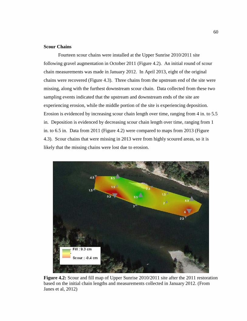
60

Scour Chains

Fourteen scour chains were installed at the Upper Sunrise 2010/2011 site

following gravel augmentation in October 2011 (Figure 4.2). An initial round of scour

chain measurements was made in January 2012. In April 2013, eight of the original

chains were recovered (Figure 4.3). Three chains from the upstream end of the site were

missing, along with the furthest downstream scour chain. Data collected from these two

sampling events indicated that the upstream and downstream ends of the site are

experiencing erosion, while the middle portion of the site is experiencing deposition.

Erosion is evidenced by increasing scour chain length over time, ranging from 4 in. to 5.5

in. Deposition is evidenced by decreasing scour chain length over time, ranging from 1

in. to 6.5 in. Data from 2011 (Figure 4.2) were compared to maps from 2013 (Figure

4.3). Scour chains that were missing in 2013 were from highly scoured areas, so it is

likely that the missing chains were lost due to erosion.

Figure 4.2: Scour and fill map of Upper Sunrise 2010/2011 site after the 2011 restoration

based on the initial chain lengths and measurements collected in January 2012. (From

Janes et al, 2012)

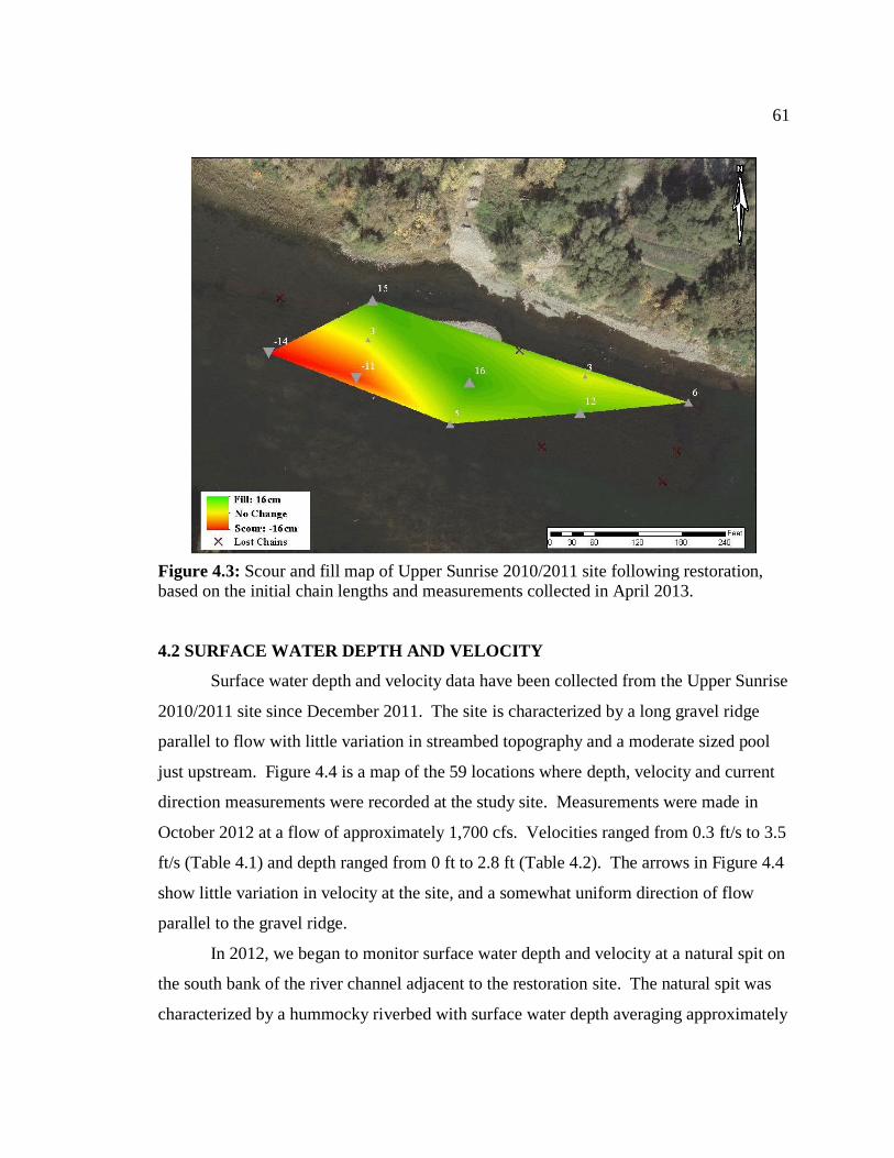
61

Figure 4.3: Scour and fill map of Upper Sunrise 2010/2011 site following restoration, based on the initial chain lengths and measurements collected in April 2013.


Surface water depth and velocity data have been collected from the Upper Sunrise

2010/2011 site since December 2011. The site is characterized by a long gravel ridge

parallel to flow with little variation in streambed topography and a moderate sized pool

just upstream. Figure 4.4 is a map of the 59 locations where depth, velocity and current

direction measurements were recorded at the study site. Measurements were made in

October 2012 at a flow of approximately 1,700 cfs. Velocities ranged from 0.3 ft/s to 3.5

ft/s (Table 4.1) and depth ranged from 0 ft to 2.8 ft (Table 4.2). The arrows in Figure 4.4

show little variation in velocity at the site, and a somewhat uniform direction of flow

parallel to the gravel ridge.

In 2012, we began to monitor surface water depth and velocity at a natural spit on

the south bank of the river channel adjacent to the restoration site. The natural spit was

characterized by a hummocky riverbed with surface water depth averaging approximately

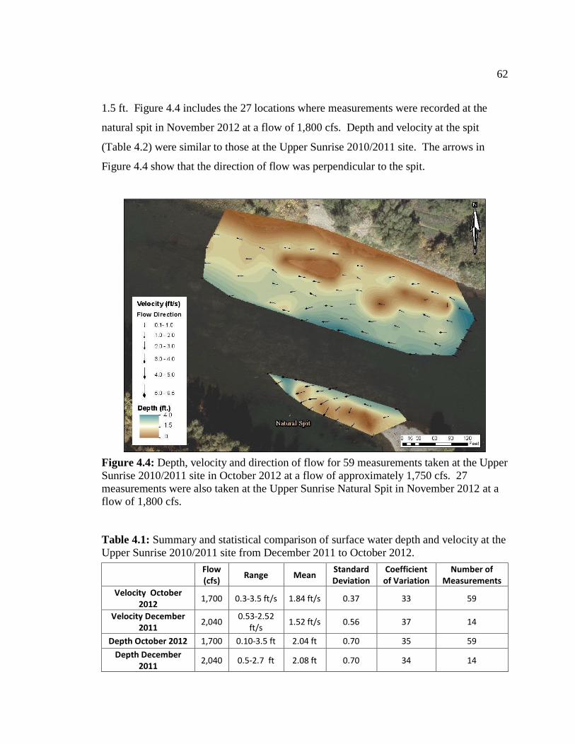
62

1.5 ft. Figure 4.4 includes the 27 locations where measurements were recorded at the

natural spit in November 2012 at a flow of 1,800 cfs. Depth and velocity at the spit

(Table 4.2) were similar to those at the Upper Sunrise 2010/2011 site. The arrows in

Figure 4.4 show that the direction of flow was perpendicular to the spit.

Figure 4.4: Depth, velocity and direction of flow for 59 measurements taken at the Upper

Sunrise 2010/2011 site in October 2012 at a flow of approximately 1,750 cfs. 27

measurements were also taken at the Upper Sunrise Natural Spit in November 2012 at a

flow of 1,800 cfs.

Table 4.1: Summary and statistical comparison of surface water depth and velocity at the

Upper Sunrise 2010/2011 site from December 2011 to October 2012.

Flow (cfs)

Range Mean Standard Deviation



Velocity October 2012

1,700 0.3-3.5 ft/s 1.84 ft/s 0.37 33 59

Velocity December 2011

2,040 0.53-2.52

ft/s 1.52 ft/s 0.56 37 14

Depth October 2012 1,700 0.10-3.5 ft 2.04 ft 0.70 35 59

Depth December 2011

2,040 0.5-2.7 ft 2.08 ft 0.70 34 14

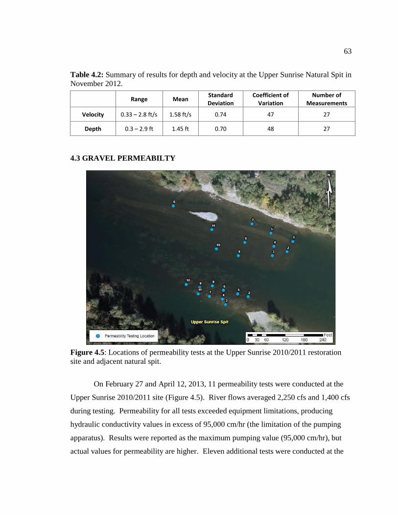
63

Table 4.2: Summary of results for depth and velocity at the Upper Sunrise Natural Spit in

November 2012.

Range Mean Standard Deviation



Velocity 0.33 – 2.8 ft/s 1.58 ft/s 0.74 47 27

Depth 0.3 – 2.9 ft 1.45 ft 0.70 48 27


Figure 4.5: Locations of permeability tests at the Upper Sunrise 2010/2011 restoration

site and adjacent natural spit.

On February 27 and April 12, 2013, 11 permeability tests were conducted at the

Upper Sunrise 2010/2011 site (Figure 4.5). River flows averaged 2,250 cfs and 1,400 cfs

during testing. Permeability for all tests exceeded equipment limitations, producing

hydraulic conductivity values in excess of 95,000 cm/hr (the limitation of the pumping

apparatus). Results were reported as the maximum pumping value (95,000 cm/hr), but

actual values for permeability are higher. Eleven additional tests were conducted at the

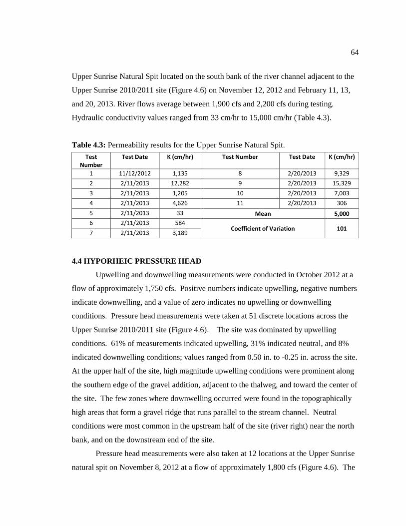
64

Upper Sunrise Natural Spit located on the south bank of the river channel adjacent to the

Upper Sunrise 2010/2011 site (Figure 4.6) on November 12, 2012 and February 11, 13,

and 20, 2013. River flows average between 1,900 cfs and 2,200 cfs during testing.

Hydraulic conductivity values ranged from 33 cm/hr to 15,000 cm/hr (Table 4.3).

Table 4.3: Permeability results for the Upper Sunrise Natural Spit.

Test Number

Test Date K (cm/hr) Test Number Test Date K (cm/hr)

1 11/12/2012 1,135 8 2/20/2013 9,329

2 2/11/2013 12,282 9 2/20/2013 15,329

3 2/11/2013 1,205 10 2/20/2013 7,003

4 2/11/2013 4,626 11 2/20/2013 306

5 2/11/2013 33 Mean 5,000

6 2/11/2013 584 Coefficient of Variation 101

7 2/11/2013 3,189


Upwelling and downwelling measurements were conducted in October 2012 at a

flow of approximately 1,750 cfs. Positive numbers indicate upwelling, negative numbers

indicate downwelling, and a value of zero indicates no upwelling or downwelling

conditions. Pressure head measurements were taken at 51 discrete locations across the

Upper Sunrise 2010/2011 site (Figure 4.6). The site was dominated by upwelling

conditions. 61% of measurements indicated upwelling, 31% indicated neutral, and 8%

indicated downwelling conditions; values ranged from 0.50 in. to -0.25 in. across the site.

At the upper half of the site, high magnitude upwelling conditions were prominent along

the southern edge of the gravel addition, adjacent to the thalweg, and toward the center of

the site. The few zones where downwelling occurred were found in the topographically

high areas that form a gravel ridge that runs parallel to the stream channel. Neutral

conditions were most common in the upstream half of the site (river right) near the north

bank, and on the downstream end of the site.

Pressure head measurements were also taken at 12 locations at the Upper Sunrise

natural spit on November 8, 2012 at a flow of approximately 1,800 cfs (Figure 4.6). The

65

spit was dominated by upwelling (58%) and neutral (42%) conditions; values ranged

from 0 in. to 0.75 in. across the site. Upwelling conditions were prominent at the

upstream half of the spit and neutral conditions at the downstream half of the spit.

Figure 4.6: Upper Sunrise 2010/2011 upwelling and downwelling data recorded on

October 25, 2012 at 1,750 cfs and natural spit data recorded on November 12, 2012

at 1,800 cfs.

4.5 TEMPERATURE

Five temperature housings (wells) were installed at both the Upper Sunrise

2010/2011 site and adjacent natural spit in April 2013 (Figure 4.7). Temperature loggers

recorded data every 30 minutes beginning on April 26, 2013. Although this report ends

in May 17, 2013, wells are still in place and will record temperature over the next year

for further study. Results from the Upper Sunrise 2010/2011 site are presented in Figures

4.8a, 4.8b, and 4.8c and results from the natural spit are presented in Figures 4.9a, 4.9b,

66

and 4.9c. Data from well US-1 is limited because the temperature loggers were

vandalized on May 4, 2013.

All wells at the Upper Sunrise 2010/2011 site showed an overall increase in

temperature during the study period regardless of depth. Diurnal temperature fluctuations

at all depths in the upstream and middle wells (US-1, US-2 and US-5) indicated strong

downwelling conditions (Figure 2.12). Well US-5 showed a slight dampening of the

diurnal tracer at 3.5 ft in the gravel indicating a slight reduction in downwelling

conditions in the middle of the site (Figure 4.8c). In the downstream wells (US-3 and

US-4), there was a distinct difference between temperatures 1 ft to 2 ft in the gravel and

those 3 ft to 4 ft into the gravel (Figure 4.8b). At shallower depths, temperatures showed

a strong diurnal signal. At greater depths, the temperature pattern showed a very weak

diurnal signal if any at all. This may indicate that groundwater is upwelling into the

shallow gravel at the downstream end of the site. This flow pattern is common in riffles,

with downwelling at the head of the riffle (pool tail-out) and upwelling at the tail of the

riffle (Stonestrom and Constantz, 2003). However, it may also indicate a change in

substrate material. During restoration, new gravel was placed directly on top of the

heavily armored streambed. This signal reduction could represent the boundary between

pre-restoration substrate and augmented gravel. Highly permeable gravel would allow

the diurnal signal to move freely at shallow depth whereas the compacted material would

reduce the ability of the diurnal signal to move through the deeper substrate. If so, the

temperature patterns from US-3 and US-4 indicate a substrate boundary between 3 ft and

4 ft deep.

All wells at the natural spit showed an overall increase in temperature during the

study period regardless of depth. Wells located on the south bank of the spit (GS-2 and

GS-4) showed a very strong upwelling signal (Figure 4.9a). Diurnal temperature

fluctuations were barely visible 1 ft. into the substrate and nonexistent at 2 ft to 4 ft

depths. Wells located on the north bank of the spit (GS-3 and GS-5) showed a slight

decrease in diurnal temperature fluctuation 1 ft in the gravel, and a highly dampened

diurnal signal below 2 ft (Figure 4.9b). This may indicate reduced upwelling conditions

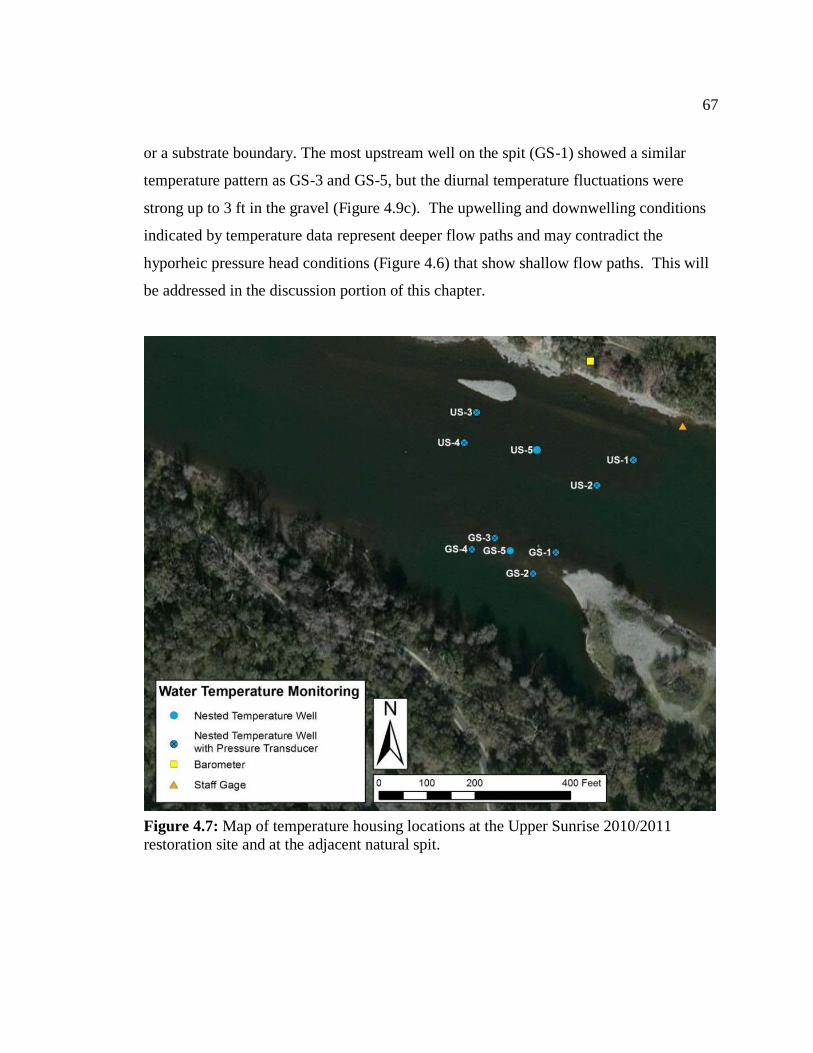
67

or a substrate boundary. The most upstream well on the spit (GS-1) showed a similar

temperature pattern as GS-3 and GS-5, but the diurnal temperature fluctuations were

strong up to 3 ft in the gravel (Figure 4.9c). The upwelling and downwelling conditions

indicated by temperature data represent deeper flow paths and may contradict the

hyporheic pressure head conditions (Figure 4.6) that show shallow flow paths. This will

be addressed in the discussion portion of this chapter.

Figure 4.7: Map of temperature housing locations at the Upper Sunrise 2010/2011

restoration site and at the adjacent natural spit.

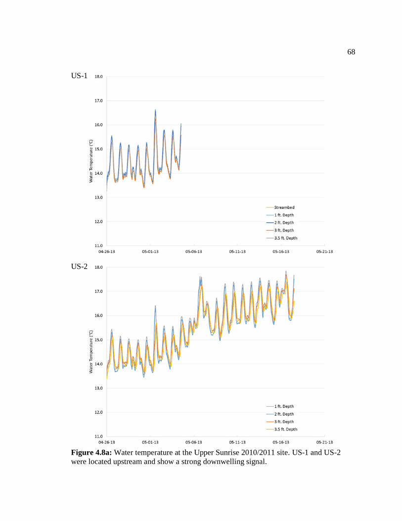
68

US-1

US-2

Figure 4.8a: Water temperature at the Upper Sunrise 2010/2011 site. US-1 and US-2

were located upstream and show a strong downwelling signal.

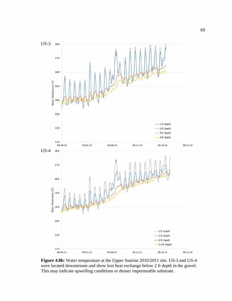
69

US-3

US-4

Figure 4.8b: Water temperature at the Upper Sunrise 2010/2011 site. US-3 and US-4

were located downstream and show less heat exchange below 2 ft depth in the gravel.

This may indicate upwelling conditions or denser impermeable substrate.

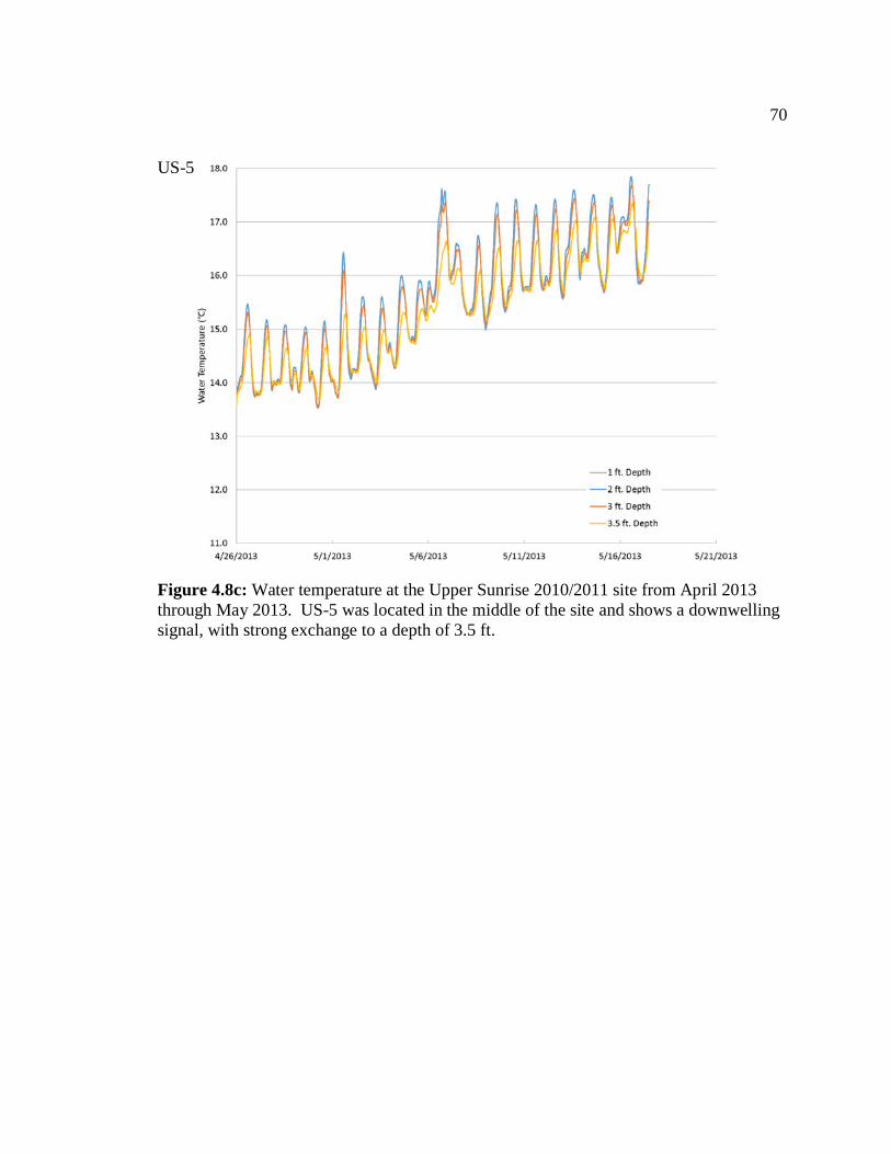
70

US-5

Figure 4.8c: Water temperature at the Upper Sunrise 2010/2011 site from April 2013

through May 2013. US-5 was located in the middle of the site and shows a downwelling

signal, with strong exchange to a depth of 3.5 ft.

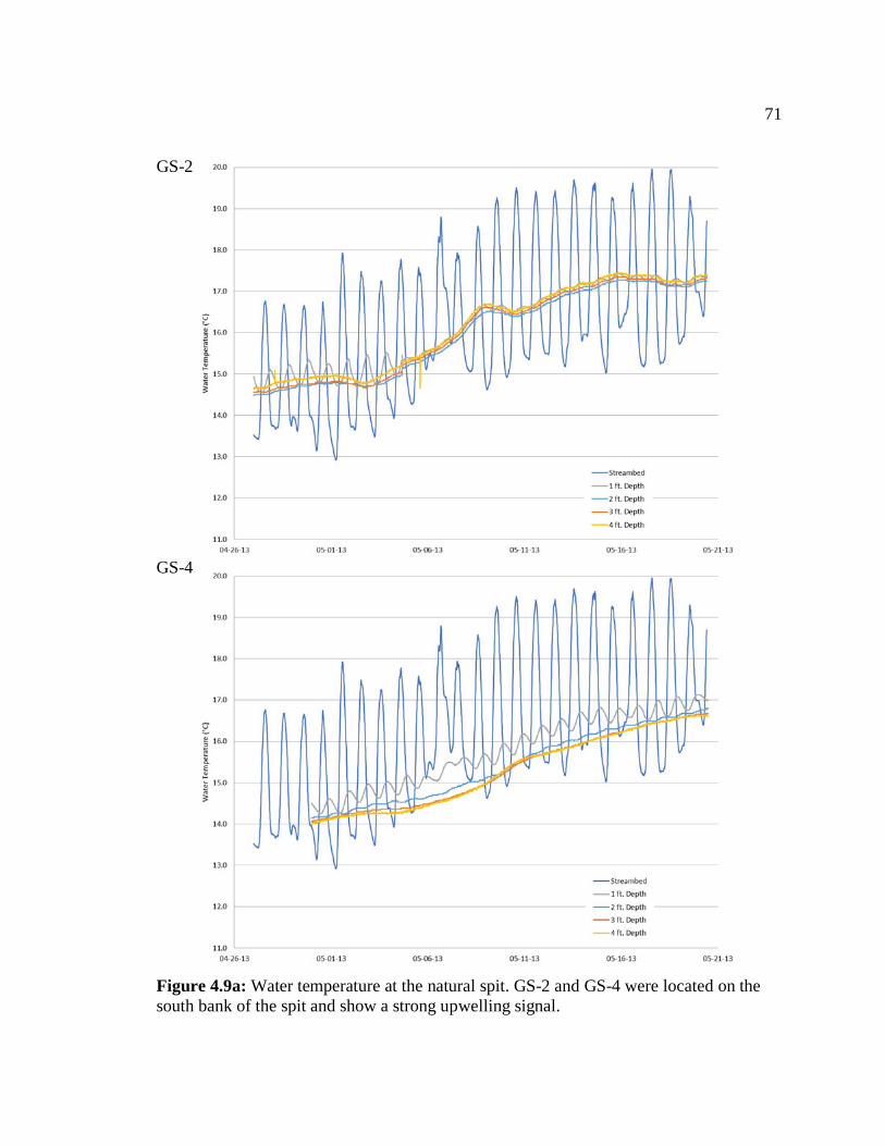
71

GS-2

GS-4

Figure 4.9a: Water temperature at the natural spit. GS-2 and GS-4 were located on the

south bank of the spit and show a strong upwelling signal.

72

GS-3

GS-5

Figure 4.9b: Water temperature at the natural spit. GS-3 and GS-5 were located on the

north bank of the spit (closest to the main channel) and show less heat exchange below 2

ft depth in the gravel. This may indicate a denser less permeable substrate 2 ft and

below.

73

GS-1

Figure 4.9c: Water temperature at the natural spit from April 2013 through May 2013.

GS-1 was located on the north bank of the spit (closest to the main channel). The GS-1

well is the most upstream well on the spit and positioned closest to the main channel.

The temperature pattern at this well shows a strong downwelling signal 1 ft to 3 ft in the

streambed and a reduced signal 4 ft in the streambed. This may indicate a less permeable

substrate 4 ft into the gravel.


Water quality parameters have been collected at the Upper Sunrise 2010/2011 site

since August 2009. Typically, post-restoration water quality samples are collected three

times within a spawning season; during redd construction in the Fall, during egg

incubation in the winter, and during fry emergence in the Spring. Discharge on the river

between December 2012 and January 2013 was high and produced flow conditions that

were unsafe for field workers (Figure 1.5). Therefore, only two sampling events were

conducted during the 2012/2013 field season, in the Fall of 2012 and the spring of 2013.

Measurements are summarized in tables and presented on maps.

74

Figure 4.10 is a location map of 16 mini-piezometers maintained at the site during

the 2012/2013 field season. Table 4.4 shows water quality data collected in November

2012 from 15 of the 16 piezometers. D.O. levels ranged from 2.62 mg/L to 10.81 mg/L

with a mean of 7.06 mg/L, and D.O. saturation ranged from 22.4% to 101.1% with a

mean of 77.2%. The well at location 8 had significantly lower intragravel flow than the

majority of the site. If the data from location 8 was classified as an outlier and removed

from the data set, then the mean D.O. level is 8.44 mg/L and the mean D.O. saturation of

81.8%. Table 4.5 shows water quality data collected in December 2011, during the

previous spawning season. D.O. levels ranged from 8.7 mg/L to 9.1 mg/L with a mean of

8.85, and percent D.O. saturation ranged from 80.3% to 85.4% with a mean of 83.68 %.

Figure 4.10: Locations of piezometers after restoration of the Upper Sunrise

2010/2011 site.

Figure 4.11 shows fall 2012 D.O. saturation levels on the Upper Sunrise

2010/2011 Map. Green dots represent high D.O. levels that are within 90% of surface

75

water levels and therefore indicate good intragravel flow. Yellow dots represent D.O.

percent levels that are within 60% -90% of surface water measurements. These sites are

reasonable for egg development and survival, but may indicate lower intragravel flow.

Red dots represent D.O. percentages that are critically low for egg development and

survival. D.O. levels were highly variable across the site.

Table 4.4: Upper Sunrise 2010/2011 Water Quality Parameters as of November 2012

Location D. O. (mg/L) D.O. (% sat) E.C. (uS) pH

Turbidity

(NTU)

1 10.22 90.03 50.7 7.15 35

2 9.8 97.5 44.1 7.1 50

3 10.46 101.1 44.5 7.1 7

4 9.89 98 47.3 6.89 80

5 4.09 39.3 58.3 6.81 90

6 7.99 79.7 44.3 6.83 170

8 2.62 22.4 55.6 6.78 6.7

9 9.81 97.4 49.3 7.08 11.9

10 10.81 99.6 48.4 7.14 77.1

11 4.89 49 42.9 6.53 58.5

12 5.07 48.5 44.8 6.57 14.1

13 9.88 97.9 48.8 7.03 3.4

14 8.31 83.2 50.8 7.06 49.1

Mean 7.06 77.2 48.4 6.93 50.2

Coefficient of Variation 36 36 10 3 94

Surface 1 10.33 101.6 44.2 7.15 5

Surface 2 10.22 100.1 46.1 7.15 4.1

Parameters were collected in November 2012 at approximately 1,800 cfs with an

average hyporheic temperature of 14.9C. Location 7 was clogged.

Areas with high and moderate D.O. values are located along the south bank (river

left) of the study area, and are closest to the thalweg. Low D.O. values were found near

the middle portion of the site where gravels are at a high elevation and form a ridge that

runs parallel to the stream channel. Figure 4.12 illustrates turbidity levels across the

study site in November 2012. Darker colors represent higher turbidity values and lighter

colors represent lower values. Turbidity levels in pore water are highly variable across

the site, ranging from 7 NTU to 170 NTU with a mean of 50.2.

Table 4.6 summarizes the mean water quality parameters before restoration of the

site (Aug. 2009) and in the years following restoration (Dec. 2011 – Apr. 2013). Prior to

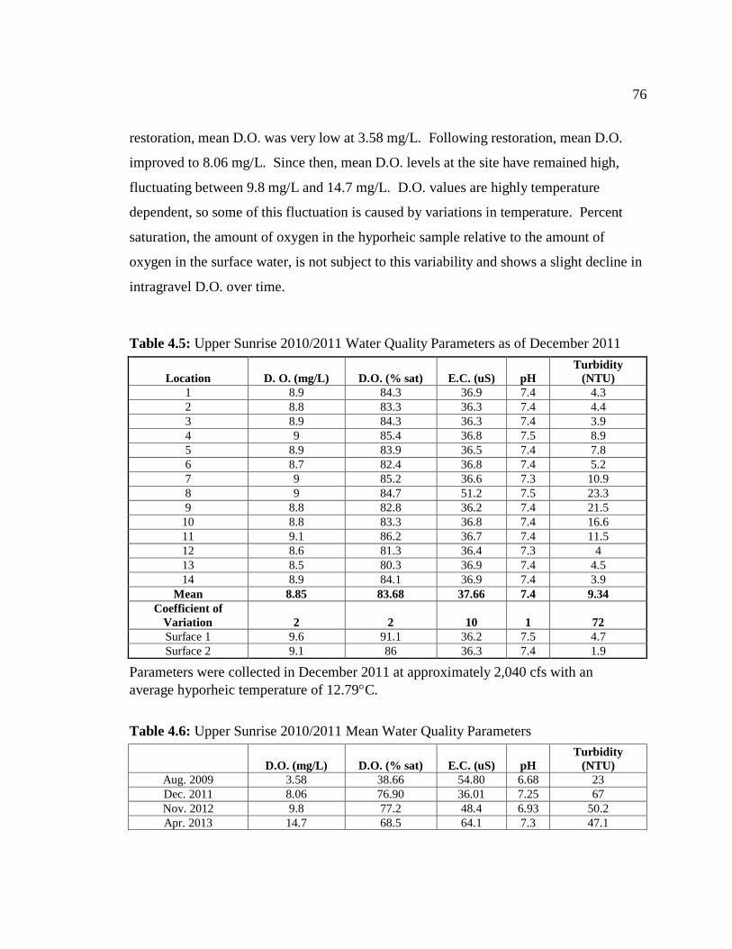
76

restoration, mean D.O. was very low at 3.58 mg/L. Following restoration, mean D.O.

improved to 8.06 mg/L. Since then, mean D.O. levels at the site have remained high,

fluctuating between 9.8 mg/L and 14.7 mg/L. D.O. values are highly temperature

dependent, so some of this fluctuation is caused by variations in temperature. Percent

saturation, the amount of oxygen in the hyporheic sample relative to the amount of

oxygen in the surface water, is not subject to this variability and shows a slight decline in

intragravel D.O. over time.

Table 4.5: Upper Sunrise 2010/2011 Water Quality Parameters as of December 2011

Location D. O. (mg/L) D.O. (% sat) E.C. (uS) pH

Turbidity

(NTU)

1 8.9 84.3 36.9 7.4 4.3

2 8.8 83.3 36.3 7.4 4.4

3 8.9 84.3 36.3 7.4 3.9

4 9 85.4 36.8 7.5 8.9

5 8.9 83.9 36.5 7.4 7.8

6 8.7 82.4 36.8 7.4 5.2

7 9 85.2 36.6 7.3 10.9

8 9 84.7 51.2 7.5 23.3

9 8.8 82.8 36.2 7.4 21.5

10 8.8 83.3 36.8 7.4 16.6

11 9.1 86.2 36.7 7.4 11.5

12 8.6 81.3 36.4 7.3 4

13 8.5 80.3 36.9 7.4 4.5

14 8.9 84.1 36.9 7.4 3.9

Mean 8.85 83.68 37.66 7.4 9.34

Coefficient of


Surface 1 9.6 91.1 36.2 7.5 4.7

Surface 2 9.1 86 36.3 7.4 1.9

Parameters were collected in December 2011 at approximately 2,040 cfs with an

average hyporheic temperature of 12.79C.

Table 4.6: Upper Sunrise 2010/2011 Mean Water Quality Parameters

D.O. (mg/L) D.O. (% sat) E.C. (uS) pH

Turbidity

(NTU)

Aug. 2009 3.58 38.66 54.80 6.68 23

Dec. 2011 8.06 76.90 36.01 7.25 67

Nov. 2012 9.8 77.2 48.4 6.93 50.2

Apr. 2013 14.7 68.5 64.1 7.3 47.1

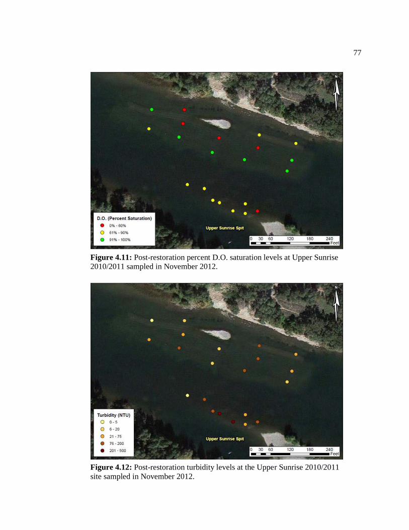
77

Figure 4.11: Post-restoration percent D.O. saturation levels at Upper Sunrise 2010/2011 sampled in November 2012.

Figure 4.12: Post-restoration turbidity levels at the Upper Sunrise 2010/2011

site sampled in November 2012.

78

4.7 DISCUSSION

Since augmentation of the Upper Sunrise 2010/2011 site in September 2011, grain

size and surface water depth and velocity have remained within optimal ranges for

salmonid spawning. Scour chain data indicated gravel was being eroded from the

upstream end and deposited along the middle portion of the site. The augmented gravel

remained highly permeable, with intragravel flow so high (>95,000 cm/hr) that the

standpipe drawdown method could not be used. Overall, hyporheic D.O. levels remained

reasonable for salmonid egg development, but showed a slight decline from December

2011 (average D.O. 8.85 mg/L) to November 2012 (average D.O. 7.06 mg/L). Turbidity

levels were highly variable in 2012, and increased significantly from December 2011

(average turbidity 9.4 NTU) to November 2012 (average turbidity 50 NTU). The slight

decrease in D.O. and strong increase in turbidity indicated that augmented gravel was just

starting to become seasoned 1.5 years after placement. The gravel was settling into a

more natural state, biofilms were emerging, and finer sediments and organic materials

were making their way into the substrate.

Upwelling and downwelling results obtained from hyporheic pressure head

measurements show shallow conditions and short flow paths, while temperature well

records at Upper Sunrise 2010/2011 provide a deeper record. Pressure head data

indicated that the majority of the shallow gravel where salmonids spawn was dominated

by upwelling conditions with a few narrow zones of neutral or downwelling conditions.

Data from the two upstream and the midstream temperature wells (Figure 4.8a: US-1,

US-2, and Figure 4.8c: US-5) indicated strong downwelling conditions in the upper

portion of the site on a broader scale. Data from the two downstream temperature wells

(Figure 4.8b: Wells US-3 and US-4) showed moderate downwelling conditions on a

broader scale. This is discussed in greater detail in chapter 7.

While physical conditions at the Upper Sunrise 2010/2011 site were within

optimal conditions for salmonid spawning, high resolution aerial images taken on

November 26, 2012 showed that the site received extremely low usage by Fall-run

Chinook salmon. Figure 4.13 shows that only six redds were observed. Four redds were

79

clustered at the uppermost boundary of the site where surface water depth ranged from

1.5 ft to 4 ft and velocities ranged between 1 ft/s and 2 ft/s. Two redds were located near

the North bank of the site where surface water depths were less than 1.5 ft and velocities

ranged from 1ft/s to 3 ft/s Direction of flow showed little variation at both locations.

This is the second spawning season since restoration, and in both years less than 15 redds

were observed at the site. Conversely, the neighboring natural spit was highly used in

both 2011 (>50 redds) and 2012 (>130 redds).

Differences in a variety of data may explain why salmon chose the natural spit

was for spawning and not the Upper Sunrise 2010/2011 site. The natural spit is

characterized by an elongated ridge of gravel that runs parallel to the main river channel

with hummocky topography. The ridge separates the main channel from a large pool on

the south bank of the river (the pool is filled by a back current of water off the main

channel). In 2012, depth and velocity averaged approximately 1.5 ft and 1.5 ft/s

respectively, and the direction of flow was perpendicular to the gravel ridge. This is

unlike the Upper Sunrise 2010/2011 site, where surface water flows parallel to the gravel

ridge. The D.O. saturation levels at the spit were in a reasonable range (60% to 90%) for

salmonid egg development, but average D.O. was lower than the Upper Sunrise

2010/2011 site.

Upwelling and downwelling results at the natural spit obtained from hyporheic

pressure head measurements show that the shallow gravel at the upstream half of the spit

was dominated by upwelling conditions and shallow gravel at the downstream half was

dominated by neutral conditions. Temperature data provided a deeper record of

intragravel flow, and indicated that downwelling was occurring on the north side of the

spit (closest to the main channel) and upwelling was occurring on the south side of the

spit (closest to the pool and south bank of the river).

Permeability measurements at the spit were highly varied. Some tests showed

surprisingly low values (33 cm/hr and 306 cm/hr), much lower than the Upper Sunrise

2010/2011 site where all values were > 95,000 cm/hr. Additionally, the average turbidity

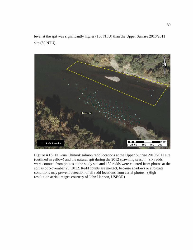
80

level at the spit was significantly higher (136 NTU) than the Upper Sunrise 2010/2011

site (50 NTU).

Figure 4.13: Fall-run Chinook salmon redd locations at the Upper Sunrise 2010/2011 site

(outlined in yellow) and the natural spit during the 2012 spawning season. Six redds

were counted from photos at the study site and 130 redds were counted from photos at the

spit as of November 26, 2012. Redd counts are inexact, because shadows or substrate

conditions may prevent detection of all redd locations from aerial photos. (High

resolution aerial images courtesy of John Hannon, USBOR)

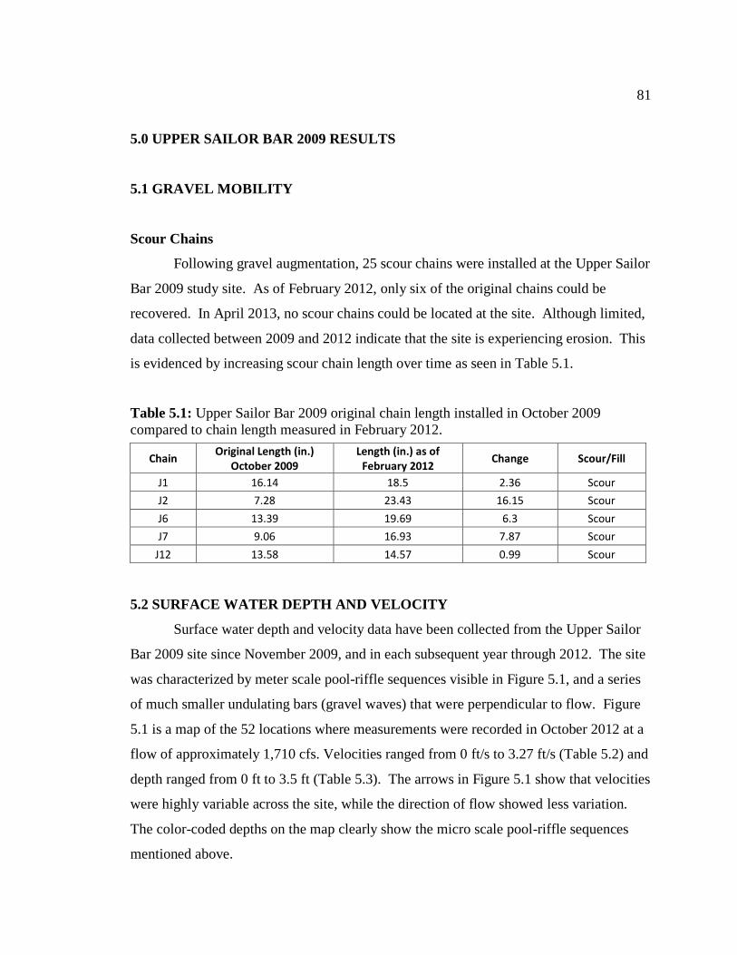
81

5.0 UPPER SAILOR BAR 2009 RESULTS

5.1 GRAVEL MOBILITY

Scour Chains

Following gravel augmentation, 25 scour chains were installed at the Upper Sailor

Bar 2009 study site. As of February 2012, only six of the original chains could be

recovered. In April 2013, no scour chains could be located at the site. Although limited,

data collected between 2009 and 2012 indicate that the site is experiencing erosion. This

is evidenced by increasing scour chain length over time as seen in Table 5.1.

Table 5.1: Upper Sailor Bar 2009 original chain length installed in October 2009

compared to chain length measured in February 2012.

Chain Original Length (in.)

October 2009 Length (in.) as of

February 2012 Change Scour/Fill

J1 16.14 18.5 2.36 Scour

J2 7.28 23.43 16.15 Scour

J6 13.39 19.69 6.3 Scour

J7 9.06 16.93 7.87 Scour

J12 13.58 14.57 0.99 Scour


Surface water depth and velocity data have been collected from the Upper Sailor

Bar 2009 site since November 2009, and in each subsequent year through 2012. The site

was characterized by meter scale pool-riffle sequences visible in Figure 5.1, and a series

of much smaller undulating bars (gravel waves) that were perpendicular to flow. Figure

5.1 is a map of the 52 locations where measurements were recorded in October 2012 at a

flow of approximately 1,710 cfs. Velocities ranged from 0 ft/s to 3.27 ft/s (Table 5.2) and

depth ranged from 0 ft to 3.5 ft (Table 5.3). The arrows in Figure 5.1 show that velocities

were highly variable across the site, while the direction of flow showed less variation.

The color-coded depths on the map clearly show the micro scale pool-riffle sequences

mentioned above.

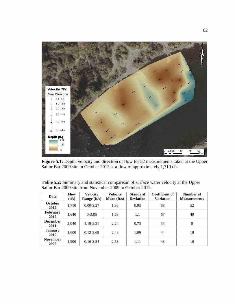
82

Figure 5.1: Depth, velocity and direction of flow for 52 measurements taken at the Upper

Sailor Bar 2009 site in October 2012 at a flow of approximately 1,710 cfs.

Table 5.2: Summary and statistical comparison of surface water velocity at the Upper

Sailor Bar 2009 site from November 2009 to October 2012.

Date Flow

(cfs)

Velocity

Range (ft/s)

Velocity

Mean (ft/s)

Standard

Deviation

Coefficient of

Variation

Number of

Measurements

October

2012 1,710 0.00-3.27 1.36 0.93 68 52

February

2012 1,640 0-3.86 1.65 1.1 67 40

December

2011 2,040 1.19-3.21 2.24 0.73 33 8

January

2010 1,600 0.12-3.69 2.48 1.09 44 10

November

2009 1,900 0.16-3.84 2.58 1.11 43 10

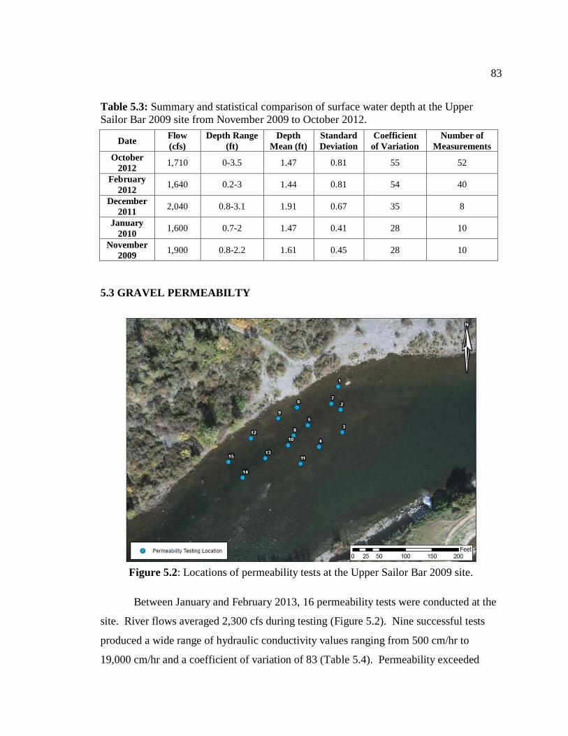
83

Table 5.3: Summary and statistical comparison of surface water depth at the Upper

Sailor Bar 2009 site from November 2009 to October 2012.

Date Flow

(cfs)

Depth Range

(ft)

Depth

Mean (ft)

Standard

Deviation

Coefficient

of Variation

Number of

Measurements

October

2012 1,710 0-3.5 1.47 0.81 55 52

February

2012 1,640 0.2-3 1.44 0.81 54 40

December

2011 2,040 0.8-3.1 1.91 0.67 35 8

January

2010 1,600 0.7-2 1.47 0.41 28 10

November

2009 1,900 0.8-2.2 1.61 0.45 28 10


Figure 5.2: Locations of permeability tests at the Upper Sailor Bar 2009 site.

Between January and February 2013, 16 permeability tests were conducted at the

site. River flows averaged 2,300 cfs during testing (Figure 5.2). Nine successful tests

produced a wide range of hydraulic conductivity values ranging from 500 cm/hr to

19,000 cm/hr and a coefficient of variation of 83 (Table 5.4). Permeability exceeded

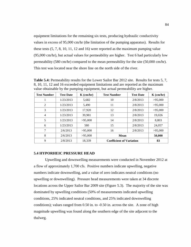
84

equipment limitations for the remaining six tests, producing hydraulic conductivity

values in excess of 95,000 cm/hr (the limitation of the pumping apparatus). Results for

these tests (5, 7, 8, 10, 11, 12 and 16) were reported as the maximum pumping value

(95,000 cm/hr), but actual values for permeability are higher. Test 6 had particularly low

permeability (580 cm/hr) compared to the mean permeability for the site (50,000 cm/hr).

This test was located near the shore line on the north side of the river.

Table 5.4: Permeability results for the Lower Sailor Bar 2012 site. Results for tests 5, 7,

8, 10, 11, 12 and 16 exceeded equipment limitations and are reported as the maximum

value obtainable by the pumping equipment, but actual permeability are higher.


1 1/23/2013 5,682 10 2/8/2013 >95,000

2 1/23/2013 5,490 11 2/8/2013 >95,000

3 1/23/2013 17,920 12 2/8/2013 >95,000

4 1/23/2013 39,981 13 2/8/2013 19,026

5 1/23/2013 >95,000 14 2/8/2013 8,803

6 1/23/2013 580 15 2/8/2013 24,057

7 2/6/2013 >95,000 16 2/8/2013 >95,000

8 2/6/2013 >95,000 Mean 50,000

9 2/8/2013 18,339 Coefficient of Variation 83


Upwelling and downwelling measurements were conducted in November 2012 at

a flow of approximately 1,700 cfs. Positive numbers indicate upwelling, negative

numbers indicate downwelling, and a value of zero indicates neutral conditions (no

upwelling or downwelling). Pressure head measurements were taken at 34 discrete

locations across the Upper Sailor Bar 2009 site (Figure 5.3). The majority of the site was

dominated by upwelling conditions (50% of measurements indicated upwelling

conditions, 25% indicated neutral conditions, and 25% indicated downwelling

conditions); values ranged from 0.50 in. to -0.50 in. across the site. A zone of high

magnitude upwelling was found along the southern edge of the site adjacent to the

thalweg.

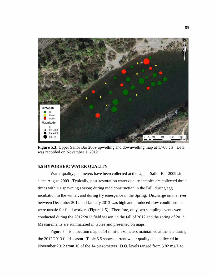
85

Figure 5.3: Upper Sailor Bar 2009 upwelling and downwelling map at 1,700 cfs. Data was recorded on November 1, 2012.


Water quality parameters have been collected at the Upper Sailor Bar 2009 site

since August 2009. Typically, post-restoration water quality samples are collected three

times within a spawning season; during redd construction in the Fall, during egg




conducted during the 2012/2013 field season, in the fall of 2012 and the spring of 2013.



the 2012/2013 field season. Table 5.5 shows current water quality data collected in

November 2012 from 10 of the 14 piezometers. D.O. levels ranged from 5.82 mg/L to

86

10.04 mg/L with a mean of 9.0 mg/L, and D.O. saturation ranged from 55.6% to 91.3%

with a mean of 87.5%. Table 5.6 shows water quality data collected in December 2011,

during the previous spawning season. D.O. levels were lower compared to 2012, ranging

from 6.0 mg/L to 9.1 mg/L with a mean of 8.06. Percent D.O. saturation was also

slightly lower in 2011, ranging from 57.2% to 82.2% with a mean of 76.9%.

Figure 5.5 shows fall 2012 D.O. saturation levels at the Upper Sailor Bar 2009

site. Green dots represent > 90% saturation and good intragravel flow. Yellow dots

represent moderate D.O. levels that are reasonable for egg development and survival but

may indicate lower intragravel flow. Red dots represent D.O. percentages that are

critically low for egg development and survival. Across the site, the majority of D.O.

saturation levels are high, a few were in the reasonable range, and only one well showed

critically low D.O. levels.

Figure 5.6 illustrates turbidity levels across the study site in November 2012.

Darker colors represent higher turbidity values and lighter colors represent lower values.

Current turbidity levels across the site are highly variable, ranging from 5 NTU to 273

NTU with a mean of 85. This is a strong increase in mean turbidity across the site when

compared to values for December 2011 (67 NTU) and November 2009 (5 NTU).


site (Aug. 2009) and in the years following restoration (Nov. 2009 – Apr. 2013). Prior to

restoration, mean D.O. was very low at 3.58 mg/L and a mean D.O. saturation of 38.66%.

Immediately following restoration, mean D.O. improved to 11.20 mg/L. Since then,

mean D.O. levels at the site have remained high, fluctuating between 8.06 mg/L and

11.45 mg/L. D.O. values are highly temperature dependent, so some of this fluctuation is

caused by variations in temperature. Percent saturation, the amount of oxygen in the

hyporheic sample relative to the amount of oxygen in the surface water, is not subject to

this variability and shows a slight decline in intragravel D.O. over time.

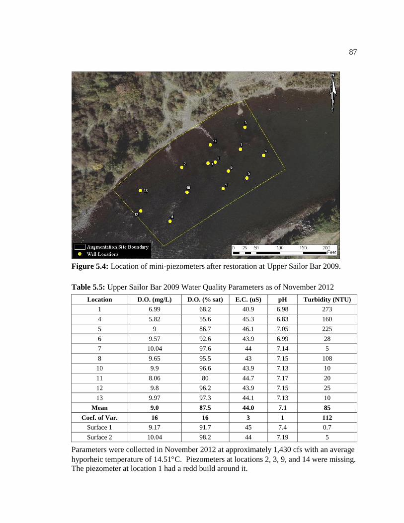
87

Figure 5.4: Location of mini-piezometers after restoration at Upper Sailor Bar 2009.

Table 5.5: Upper Sailor Bar 2009 Water Quality Parameters as of November 2012


1 6.99 68.2 40.9 6.98 273

4 5.82 55.6 45.3 6.83 160

5 9 86.7 46.1 7.05 225

6 9.57 92.6 43.9 6.99 28

7 10.04 97.6 44 7.14 5

8 9.65 95.5 43 7.15 108

10 9.9 96.6 43.9 7.13 10

11 8.06 80 44.7 7.17 20

12 9.8 96.2 43.9 7.15 25

13 9.97 97.3 44.1 7.13 10

Mean 9.0 87.5 44.0 7.1 85

Coef. of Var. 16 16 3 1 112

Surface 1 9.17 91.7 45 7.4 0.7

Surface 2 10.04 98.2 44 7.19 5

Parameters were collected in November 2012 at approximately 1,430 cfs with an average

hyporheic temperature of 14.51C. Piezometers at locations 2, 3, 9, and 14 were missing.

The piezometer at location 1 had a redd build around it.

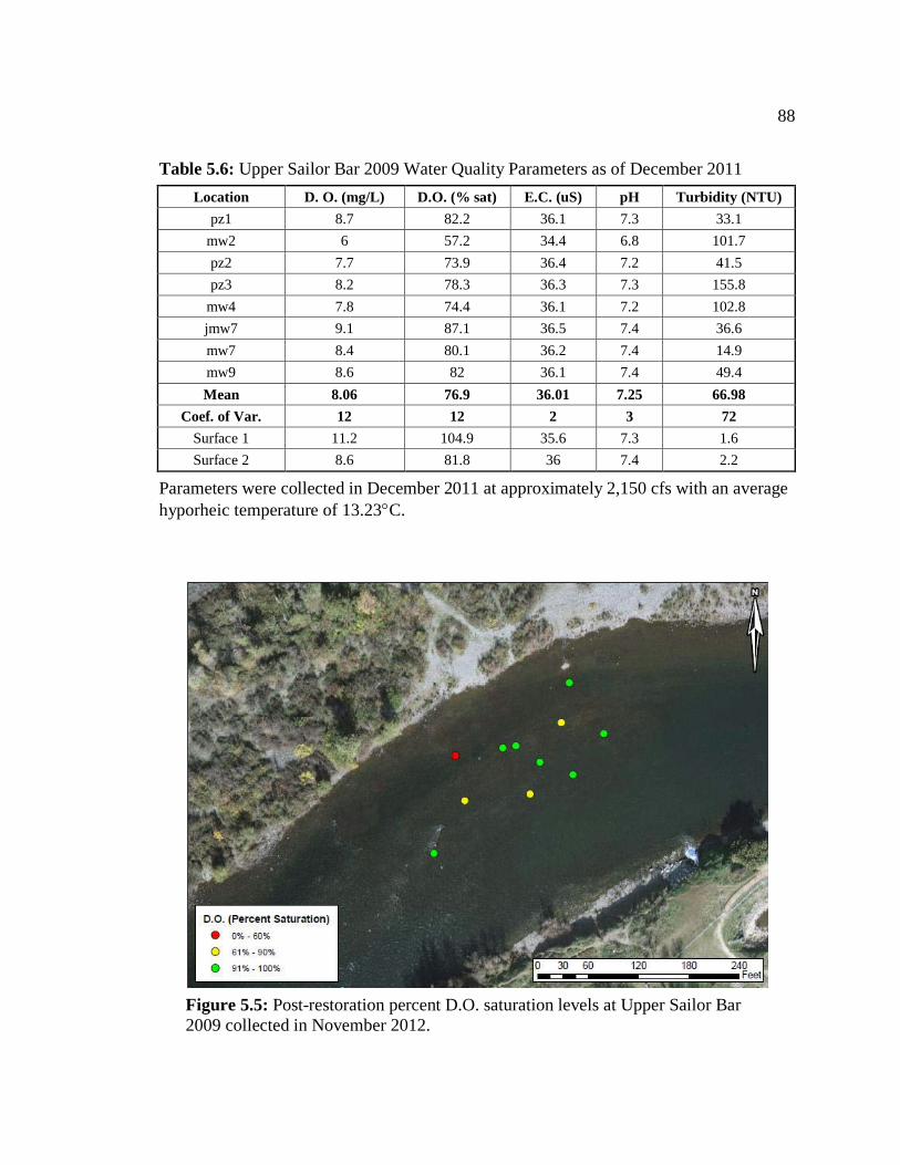
88

Table 5.6: Upper Sailor Bar 2009 Water Quality Parameters as of December 2011

Location D. O. (mg/L) D.O. (% sat) E.C. (uS) pH Turbidity (NTU)

pz1 8.7 82.2 36.1 7.3 33.1

mw2 6 57.2 34.4 6.8 101.7

pz2 7.7 73.9 36.4 7.2 41.5

pz3 8.2 78.3 36.3 7.3 155.8

mw4 7.8 74.4 36.1 7.2 102.8

jmw7 9.1 87.1 36.5 7.4 36.6

mw7 8.4 80.1 36.2 7.4 14.9

mw9 8.6 82 36.1 7.4 49.4

Mean 8.06 76.9 36.01 7.25 66.98

Coef. of Var. 12 12 2 3 72

Surface 1 11.2 104.9 35.6 7.3 1.6

Surface 2 8.6 81.8 36 7.4 2.2

Parameters were collected in December 2011 at approximately 2,150 cfs with an average

hyporheic temperature of 13.23C.

Figure 5.5: Post-restoration percent D.O. saturation levels at Upper Sailor Bar

2009 collected in November 2012.

89

Figure 5.6: Post-restoration turbidity levels at Upper Sailor Bar 2009 collected in

November 2012.

Table 5.7: Upper Sailor Bar 2009 Mean Water Quality Parameters

D.O. (mg/L) D.O. (% sat) E.C. (uS) pH Turbidity (NTU)

Aug. 2009 3.58 38.66 54.80 6.68 23

Nov. 2009 11.20 95.73 52.20 7.20 5

Jan. 2010 11.45 99.79 58.30 7.20 5

Dec. 2011 8.06 76.90 36.01 7.25 67

Feb. 2012 10.00 84.00 43.40 7.30 65

Nov. 2012 9.00 87.50 44.00 7.10 85

Apr. 2013 8.82 86.00 22.80 7.40 56

5.6 DISCUSSION

Grain size and surface water depth and velocity have remained within optimal

ranges for salmonid spawning since augmentation of the Upper Sailor Bar 2009 site in

August 2009. Scour chain data indicated that gravel was eroded throughout the site. The

site was dominated by upwelling conditions. Permeability was highly variable ranging

from < 580 cm/hr to 19,000 cm/hr. Between November 2009 (immediately following

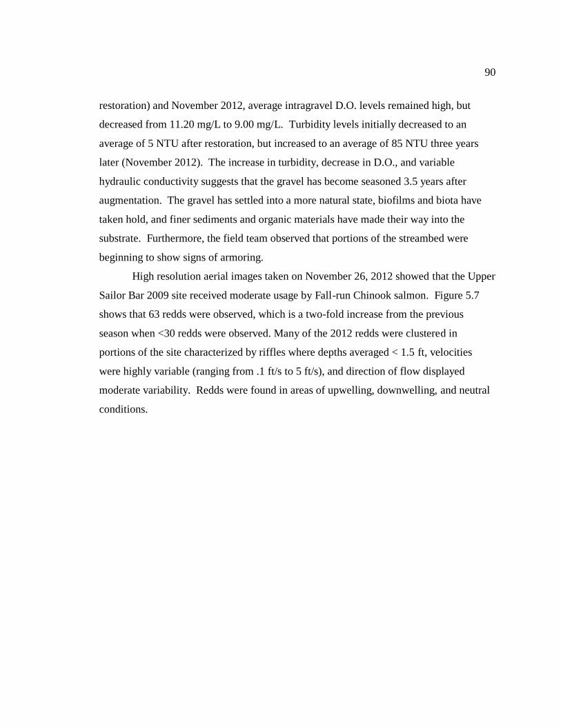
90

restoration) and November 2012, average intragravel D.O. levels remained high, but

decreased from 11.20 mg/L to 9.00 mg/L. Turbidity levels initially decreased to an

average of 5 NTU after restoration, but increased to an average of 85 NTU three years

later (November 2012). The increase in turbidity, decrease in D.O., and variable

hydraulic conductivity suggests that the gravel has become seasoned 3.5 years after

augmentation. The gravel has settled into a more natural state, biofilms and biota have

taken hold, and finer sediments and organic materials have made their way into the

substrate. Furthermore, the field team observed that portions of the streambed were

beginning to show signs of armoring.

High resolution aerial images taken on November 26, 2012 showed that the Upper

Sailor Bar 2009 site received moderate usage by Fall-run Chinook salmon. Figure 5.7

shows that 63 redds were observed, which is a two-fold increase from the previous

season when <30 redds were observed. Many of the 2012 redds were clustered in

portions of the site characterized by riffles where depths averaged < 1.5 ft, velocities

were highly variable (ranging from .1 ft/s to 5 ft/s), and direction of flow displayed

moderate variability. Redds were found in areas of upwelling, downwelling, and neutral

conditions.

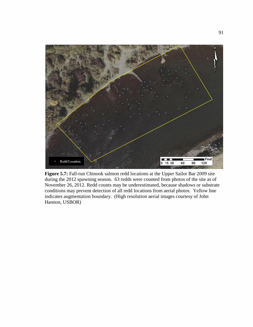
91

Figure 5.7: Fall-run Chinook salmon redd locations at the Upper Sailor Bar 2009 site during the 2012 spawning season. 63 redds were counted from photos of the site as of

November 26, 2012. Redd counts may be underestimated, because shadows or substrate

conditions may prevent detection of all redd locations from aerial photos. Yellow line

indicates augmentation boundary. (High resolution aerial images courtesy of John

Hannon, USBOR)

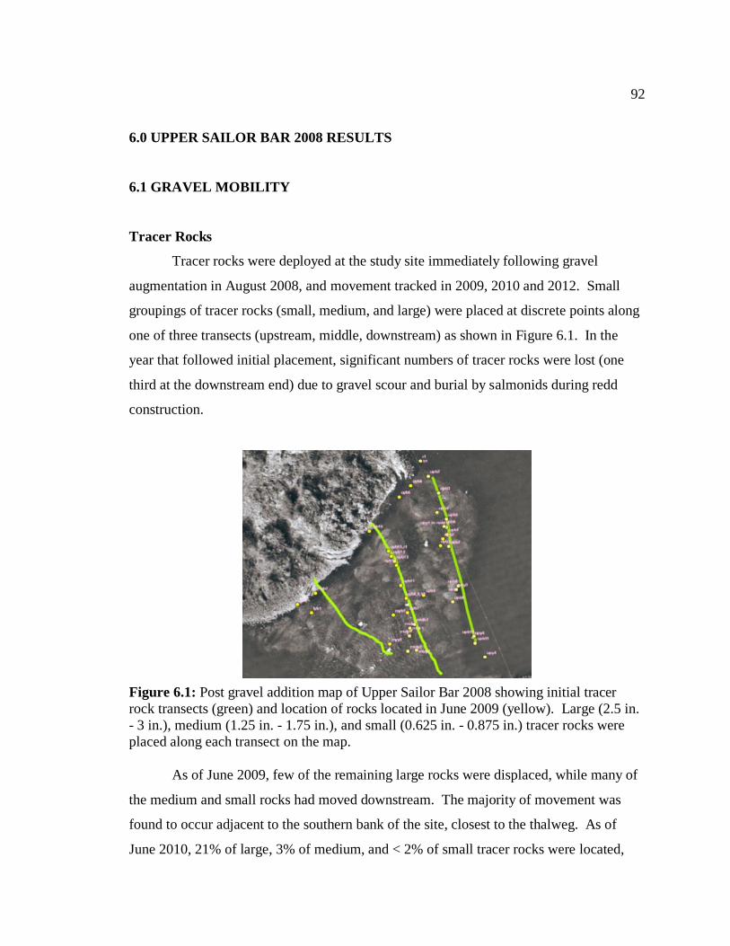
92

6.0 UPPER SAILOR BAR 2008 RESULTS

6.1 GRAVEL MOBILITY

Tracer Rocks

Tracer rocks were deployed at the study site immediately following gravel

augmentation in August 2008, and movement tracked in 2009, 2010 and 2012. Small

groupings of tracer rocks (small, medium, and large) were placed at discrete points along

one of three transects (upstream, middle, downstream) as shown in Figure 6.1. In the

year that followed initial placement, significant numbers of tracer rocks were lost (one

third at the downstream end) due to gravel scour and burial by salmonids during redd

construction.

Figure 6.1: Post gravel addition map of Upper Sailor Bar 2008 showing initial tracer

rock transects (green) and location of rocks located in June 2009 (yellow). Large (2.5 in.

- 3 in.), medium (1.25 in. - 1.75 in.), and small (0.625 in. - 0.875 in.) tracer rocks were

placed along each transect on the map.

As of June 2009, few of the remaining large rocks were displaced, while many of

the medium and small rocks had moved downstream. The majority of movement was

found to occur adjacent to the southern bank of the site, closest to the thalweg. As of

June 2010, 21% of large, 3% of medium, and < 2% of small tracer rocks were located,

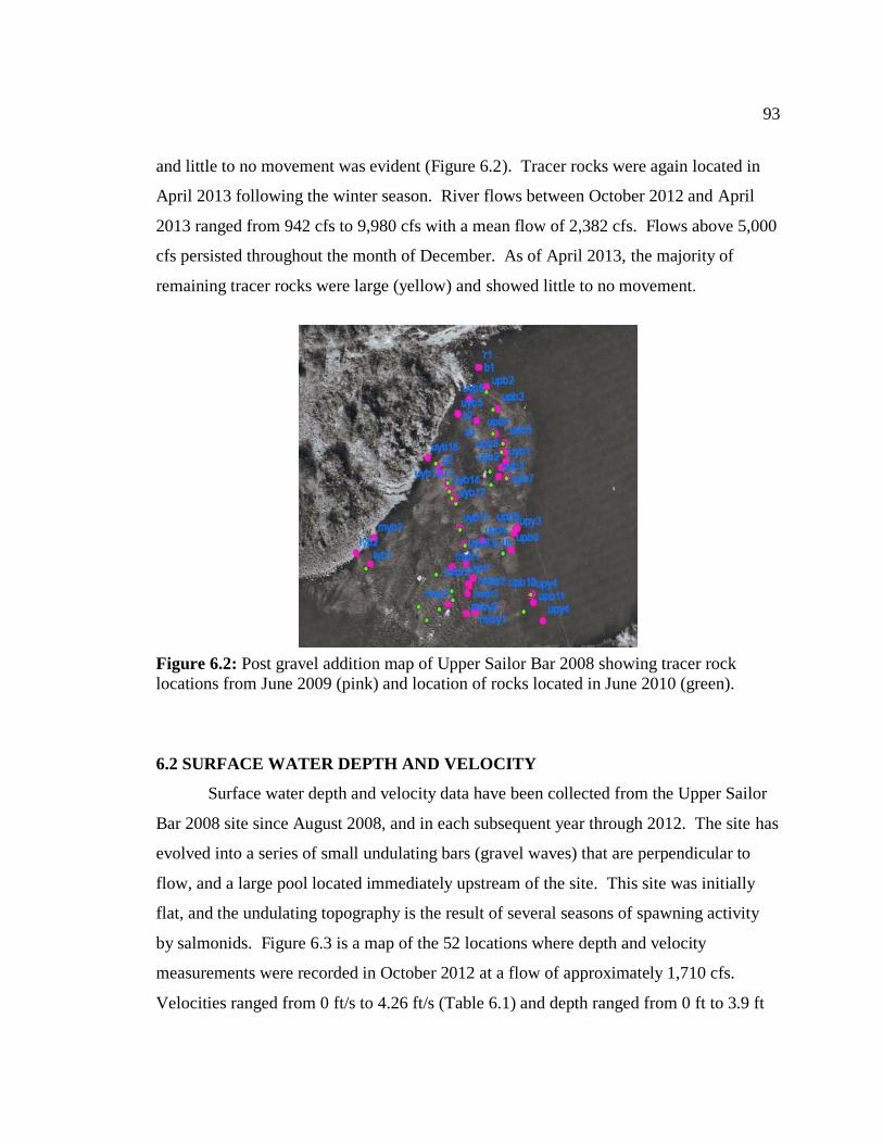
93

and little to no movement was evident (Figure 6.2). Tracer rocks were again located in

April 2013 following the winter season. River flows between October 2012 and April

2013 ranged from 942 cfs to 9,980 cfs with a mean flow of 2,382 cfs. Flows above 5,000

cfs persisted throughout the month of December. As of April 2013, the majority of

remaining tracer rocks were large (yellow) and showed little to no movement.

Figure 6.2: Post gravel addition map of Upper Sailor Bar 2008 showing tracer rock

locations from June 2009 (pink) and location of rocks located in June 2010 (green).


Surface water depth and velocity data have been collected from the Upper Sailor

Bar 2008 site since August 2008, and in each subsequent year through 2012. The site has

evolved into a series of small undulating bars (gravel waves) that are perpendicular to

flow, and a large pool located immediately upstream of the site. This site was initially

flat, and the undulating topography is the result of several seasons of spawning activity

by salmonids. Figure 6.3 is a map of the 52 locations where depth and velocity

measurements were recorded in October 2012 at a flow of approximately 1,710 cfs.

Velocities ranged from 0 ft/s to 4.26 ft/s (Table 6.1) and depth ranged from 0 ft to 3.9 ft

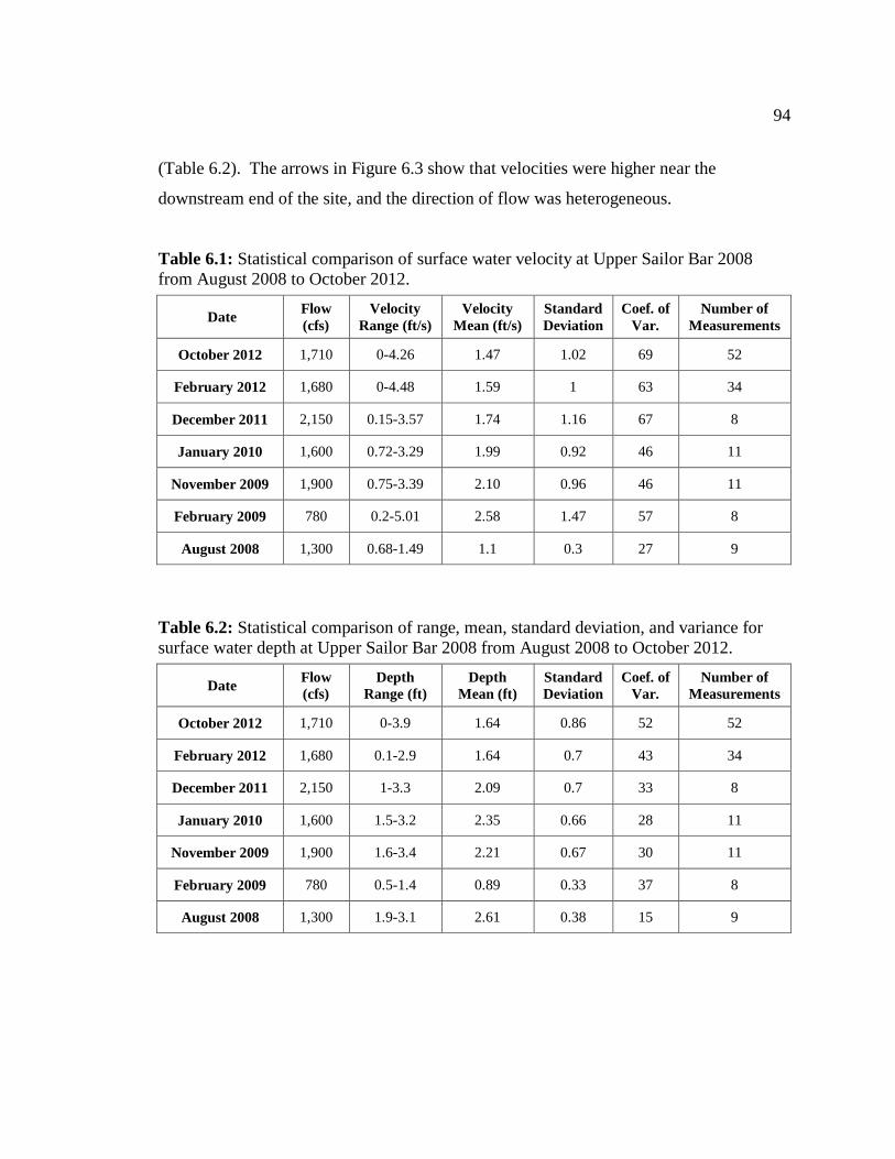
94

(Table 6.2). The arrows in Figure 6.3 show that velocities were higher near the

downstream end of the site, and the direction of flow was heterogeneous.

Table 6.1: Statistical comparison of surface water velocity at Upper Sailor Bar 2008

from August 2008 to October 2012.

Date Flow

(cfs)

Velocity

Range (ft/s)

Velocity

Mean (ft/s)

Standard

Deviation

Coef. of

Var.

Number of

Measurements

October 2012 1,710 0-4.26 1.47 1.02 69 52

February 2012 1,680 0-4.48 1.59 1 63 34

December 2011 2,150 0.15-3.57 1.74 1.16 67 8

January 2010 1,600 0.72-3.29 1.99 0.92 46 11

November 2009 1,900 0.75-3.39 2.10 0.96 46 11

February 2009 780 0.2-5.01 2.58 1.47 57 8

August 2008 1,300 0.68-1.49 1.1 0.3 27 9

Table 6.2: Statistical comparison of range, mean, standard deviation, and variance for

surface water depth at Upper Sailor Bar 2008 from August 2008 to October 2012.

Date Flow

(cfs)

Depth

Range (ft)

Depth

Mean (ft)

Standard

Deviation

Coef. of

Var.

Number of

Measurements

October 2012 1,710 0-3.9 1.64 0.86 52 52

February 2012 1,680 0.1-2.9 1.64 0.7 43 34

December 2011 2,150 1-3.3 2.09 0.7 33 8

January 2010 1,600 1.5-3.2 2.35 0.66 28 11

November 2009 1,900 1.6-3.4 2.21 0.67 30 11

February 2009 780 0.5-1.4 0.89 0.33 37 8

August 2008 1,300 1.9-3.1 2.61 0.38 15 9

95

Figure 6.3: Depth, velocity and direction of flow for 52 measurements taken at

Upper Sailor Bar 2008 in October 2012 at a flow of approximately 1,710 cfs.


On February 22 and February 25, 2013, 17 permeability tests were conducted at

the Upper Sailor Bar 2008 site (Figure 6.4). River flows averaged 2,500 cfs during

testing. Fifteen successful tests produced highly variable hydraulic conductivity values

ranging from 1 cm/hr to 19,000 cm/hr and a coefficient of variation of 179 (Table 6.3).

Fifteen successful tests produced a wide range of hydraulic conductivity values ranging

from < 1 cm/hr to >19,000 cm/hr with a 90.34% coefficient of variation (Table 6.3).

Permeability exceeded equipment limitations for the remaining two tests, producing

hydraulic conductivity values in excess of 95,000 cm/hr (the limitation of the pumping

apparatus). Results for these tests (6 and 14) were reported as the maximum pumping

value (95,000 cm/hr), but actual values for permeability are higher. Tests 2, 12, and 17

had extremely low permeability (< 1 cm/hr). Two of these tests (12 and 17) were located

closest to the shore line on the north bank of the river. Test 2 was the furthest upstream

location measured.

96

Figure 6.4: Locations of permeability tests at Lower Sailor Bar 2008.

Table 6.3: Permeability results for Upper Sailor Bar 2008. Results for tests 6 and 14

exceeded equipment limitations and are reported as the maximum value obtainable by the

pumping equipment, but actual permeability are higher.


1 2/22/2013 5,376 11 2/25/2013 2,512

2 2/22/2013 1 12 2/25/2013 1

3 2/22/2013 14,906 13 2/25/2013 3,587

4 2/22/2013 626 14 2/25/2013 >95,000

5 2/22/2013 773 15 2/25/2013 19,214

6 2/22/2013 >95,000 16 2/25/2013 18,120

7 2/22/2013 6,002 17 2/25/2013 1

8 2/22/2013 7,281 Mean 17,000

9 2/25/2013 1,832 Coefficient of Variation 179

10 2/25/2013 15,643

Upstream

Downstream

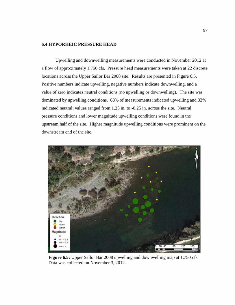
97


Upwelling and downwelling measurements were conducted in November 2012 at

a flow of approximately 1,750 cfs. Pressure head measurements were taken at 22 discrete

locations across the Upper Sailor Bar 2008 site. Results are presented in Figure 6.5.

Positive numbers indicate upwelling, negative numbers indicate downwelling, and a

value of zero indicates neutral conditions (no upwelling or downwelling). The site was

dominated by upwelling conditions. 68% of measurements indicated upwelling and 32%

indicated neutral; values ranged from 1.25 in. to -0.25 in. across the site. Neutral

pressure conditions and lower magnitude upwelling conditions were found in the

upstream half of the site. Higher magnitude upwelling conditions were prominent on the

downstream end of the site.

Figure 6.5: Upper Sailor Bar 2008 upwelling and downwelling map at 1,750 cfs.

Data was collected on November 3, 2012.

98


Water quality parameters have been collected at the Upper Sailor Bar 2008 site

since September 2008. Typically, post-restoration water quality samples are collected

three times within a spawning season; during redd construction in the Fall, during egg




conducted during the 2012/2013 field season (in the fall 2012 and spring 2013).



the 2012/2013 field season. Table 6.4 shows current water quality data collected in

November 2012 from nine of the 13 piezometers. D.O. levels ranged from 3.75 mg/L to

9.49 mg/L with a mean of 7.98 mg/L, and D.O. saturation ranged from 43% to 91.3%

with a mean of 77.76%. Table 6.5 shows water quality data collected during the previous

spawning season (December 2011). D.O. levels were similar to 2012, ranging from 3.4

mg/L to 9.0 mg/L with a mean of 7.46 mg/L. Percent D.O. saturation was slightly lower,

ranging from 31.5% to 84.3% with a mean of 69.5%.

99

Figure 6.6: Piezometer locations after restoration at the Upper Sailor Bar 2008 site.

Table 6.4: Upper Sailor Bar 2008 Water Quality Parameters as of November 2012

Location D.O. (mg/L) D.O. (% sat) E.C. (uS) pH

Turbidity

(NTU)

1 6.7 57.4 47.5 7.04 180

2 8.28 81.7 53.9 7.27 120

3 3.75 43 128.6 7.1 400

4 9.22 88.4 44.2 7.14 60

5 6.84 66 44.2 7.14 60

6 9.04 88.9 44.1 7.02 9

7 9.37 91.3 43.8 7.01 5

8 9.16 90.1 43.9 7.19 15

10 9.49 93 43.9 7.19 15

Mean 7.98 77.76 54.90 7.12 96


Surface 1 9.17 91.7 45 7.4 15

Surface 2 10.04 98.2 44 7.19 14.4

Parameters were collected in November 2012 at approximately 1,430 cfs with an average

hyporheic temperature of 14.5C. Piezometers 12 and 13 were missing; 9 and 11 were

clogged.

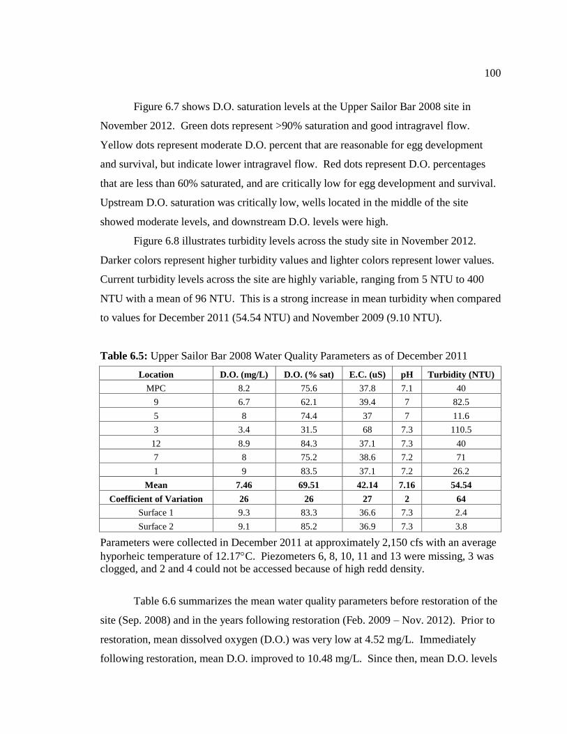
100

Figure 6.7 shows D.O. saturation levels at the Upper Sailor Bar 2008 site in

November 2012. Green dots represent >90% saturation and good intragravel flow.

Yellow dots represent moderate D.O. percent that are reasonable for egg development

and survival, but indicate lower intragravel flow. Red dots represent D.O. percentages

that are less than 60% saturated, and are critically low for egg development and survival.

Upstream D.O. saturation was critically low, wells located in the middle of the site

showed moderate levels, and downstream D.O. levels were high.

Figure 6.8 illustrates turbidity levels across the study site in November 2012.

Darker colors represent higher turbidity values and lighter colors represent lower values.

Current turbidity levels across the site are highly variable, ranging from 5 NTU to 400

NTU with a mean of 96 NTU. This is a strong increase in mean turbidity when compared

to values for December 2011 (54.54 NTU) and November 2009 (9.10 NTU).

Table 6.5: Upper Sailor Bar 2008 Water Quality Parameters as of December 2011


MPC 8.2 75.6 37.8 7.1 40

9 6.7 62.1 39.4 7 82.5

5 8 74.4 37 7 11.6

3 3.4 31.5 68 7.3 110.5

12 8.9 84.3 37.1 7.3 40

7 8 75.2 38.6 7.2 71

1 9 83.5 37.1 7.2 26.2

Mean 7.46 69.51 42.14 7.16 54.54


Surface 1 9.3 83.3 36.6 7.3 2.4

Surface 2 9.1 85.2 36.9 7.3 3.8

Parameters were collected in December 2011 at approximately 2,150 cfs with an average

hyporheic temperature of 12.17C. Piezometers 6, 8, 10, 11 and 13 were missing, 3 was clogged, and 2 and 4 could not be accessed because of high redd density.


site (Sep. 2008) and in the years following restoration (Feb. 2009 – Nov. 2012). Prior to

restoration, mean dissolved oxygen (D.O.) was very low at 4.52 mg/L. Immediately

following restoration, mean D.O. improved to 10.48 mg/L. Since then, mean D.O. levels

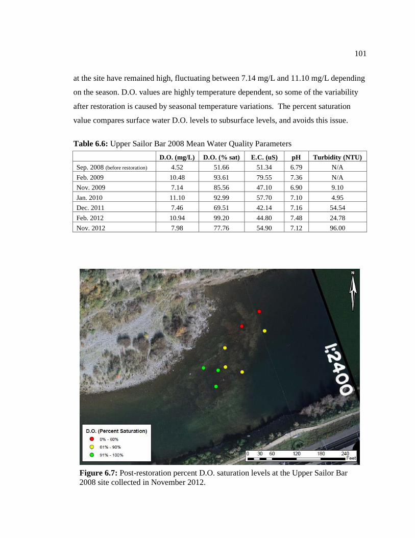
101

at the site have remained high, fluctuating between 7.14 mg/L and 11.10 mg/L depending

on the season. D.O. values are highly temperature dependent, so some of the variability

after restoration is caused by seasonal temperature variations. The percent saturation

value compares surface water D.O. levels to subsurface levels, and avoids this issue.

Table 6.6: Upper Sailor Bar 2008 Mean Water Quality Parameters

D.O. (mg/L) D.O. (% sat) E.C. (uS) pH Turbidity (NTU)

Sep. 2008 (before restoration) 4.52 51.66 51.34 6.79 N/A

Feb. 2009 10.48 93.61 79.55 7.36 N/A

Nov. 2009 7.14 85.56 47.10 6.90 9.10

Jan. 2010 11.10 92.99 57.70 7.10 4.95

Dec. 2011 7.46 69.51 42.14 7.16 54.54

Feb. 2012 10.94 99.20 44.80 7.48 24.78

Nov. 2012 7.98 77.76 54.90 7.12 96.00

Figure 6.7: Post-restoration percent D.O. saturation levels at the Upper Sailor Bar

2008 site collected in November 2012.

102

Figure 6.8: Post-restoration turbidity levels at Upper Sailor Bar 2008 collected in November 2012.

6.6 DISSCUSSION

Grain size and surface water depth and velocity have remained within optimal

range for salmonid spawning since augmentation of the Upper Sailor Bar 2008 site in

September 2008. Most of the original tracer rocks deployed at the site have been lost,

and those recovered in April 2013 showed little to no movement between 2012 and 2013.

Five years after restoration, the site was dominated by upwelling conditions, and the

permeability was generally high with an average of 17,000 cm/hr. Between February

2009 and November 2012, intragravel D.O. levels decreased and became more variable.

D.O. values ranged from 10.0 mg/L to 11.0 mg/L in February 2009 and 3.75 mg/L to

9.49 mg/L in November 2012. Turbidity was not measured at the site until one year after

gravel placement (November 2009). Since then, turbidity levels have increased from an

average of 9.10 NTU in November 2009 to 96.00 NTU in November 2012.

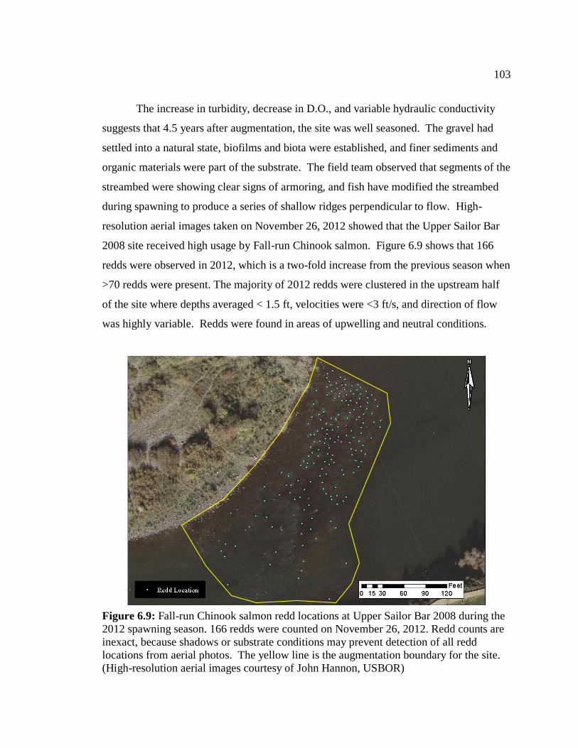
103

The increase in turbidity, decrease in D.O., and variable hydraulic conductivity

suggests that 4.5 years after augmentation, the site was well seasoned. The gravel had

settled into a natural state, biofilms and biota were established, and finer sediments and

organic materials were part of the substrate. The field team observed that segments of the

streambed were showing clear signs of armoring, and fish have modified the streambed

during spawning to produce a series of shallow ridges perpendicular to flow. High-

resolution aerial images taken on November 26, 2012 showed that the Upper Sailor Bar

2008 site received high usage by Fall-run Chinook salmon. Figure 6.9 shows that 166

redds were observed in 2012, which is a two-fold increase from the previous season when

>70 redds were present. The majority of 2012 redds were clustered in the upstream half

of the site where depths averaged < 1.5 ft, velocities were <3 ft/s, and direction of flow

was highly variable. Redds were found in areas of upwelling and neutral conditions.

Figure 6.9: Fall-run Chinook salmon redd locations at Upper Sailor Bar 2008 during the

2012 spawning season. 166 redds were counted on November 26, 2012. Redd counts are

inexact, because shadows or substrate conditions may prevent detection of all redd

locations from aerial photos. The yellow line is the augmentation boundary for the site.

(High-resolution aerial images courtesy of John Hannon, USBOR)

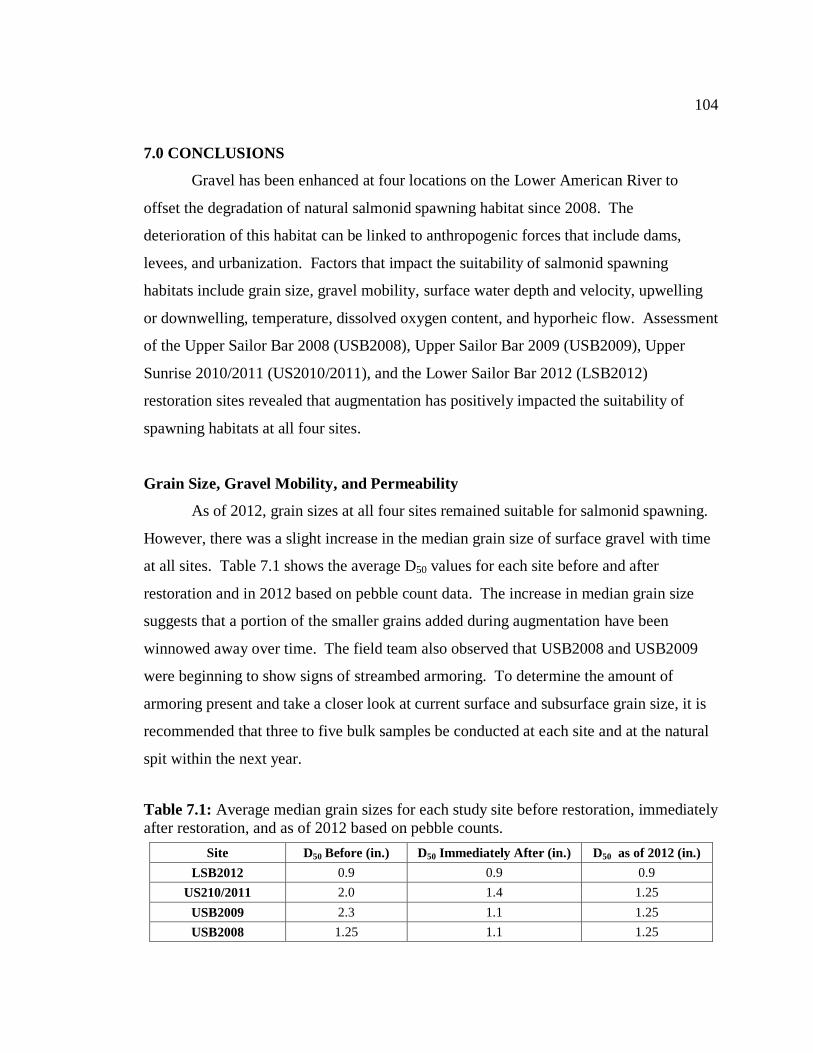
104

7.0 CONCLUSIONS

Gravel has been enhanced at four locations on the Lower American River to

offset the degradation of natural salmonid spawning habitat since 2008. The

deterioration of this habitat can be linked to anthropogenic forces that include dams,

levees, and urbanization. Factors that impact the suitability of salmonid spawning

habitats include grain size, gravel mobility, surface water depth and velocity, upwelling

or downwelling, temperature, dissolved oxygen content, and hyporheic flow. Assessment

of the Upper Sailor Bar 2008 (USB2008), Upper Sailor Bar 2009 (USB2009), Upper

Sunrise 2010/2011 (US2010/2011), and the Lower Sailor Bar 2012 (LSB2012)

restoration sites revealed that augmentation has positively impacted the suitability of

spawning habitats at all four sites.

Grain Size, Gravel Mobility, and Permeability

As of 2012, grain sizes at all four sites remained suitable for salmonid spawning.

However, there was a slight increase in the median grain size of surface gravel with time

at all sites. Table 7.1 shows the average D50 values for each site before and after

restoration and in 2012 based on pebble count data. The increase in median grain size

suggests that a portion of the smaller grains added during augmentation have been

winnowed away over time. The field team also observed that USB2008 and USB2009

were beginning to show signs of streambed armoring. To determine the amount of

armoring present and take a closer look at current surface and subsurface grain size, it is

recommended that three to five bulk samples be conducted at each site and at the natural

spit within the next year.

Table 7.1: Average median grain sizes for each study site before restoration, immediately

after restoration, and as of 2012 based on pebble counts.

Site D50 Before (in.) D50 Immediately After (in.) D50 as of 2012 (in.)

LSB2012 0.9 0.9 0.9

US210/2011 2.0 1.4 1.25

USB2009 2.3 1.1 1.25

USB2008 1.25 1.1 1.25

105

Because suitable spawning gravel is highly mobile, sediment transport is expected

over time. Cumulative data collected from scour chains and tracer rocks indicated

downstream movement of gravel at all four restoration sites. The majority of movement

seen at the older sites occurred in the first two years following restoration. Little to no

movement was seen at the USB2008 site between 2011 and 2013, and the loss of all

scour chains at USB2009 makes it difficult to determine erosion or deposition patterns

between 2012 and 2013 (four years after restoration). Both US2010/2011 and LSB2012

showed upstream erosion and mid or downstream deposition. However, the loss of

multiple scour chains at US2010/2011, and LSB2012 makes it difficult to accurately

assess sediment transport patterns. The missing scour chains leave a hole in the data that

is an important piece to understanding the longevity of augmentation sites. Further study

is necessary to fully understand sediment transport at restoration sites, and it is suggested

that the following recommendations be employed to assess gravel mobility in the future:

(1) Have a field team visit each site during the next low flow event and dig out areas

where scour chains should be located. At the moment, it is not clear if the scour

chains have been released due to erosion or completely buried from deposition.

(2) Replace missing scour chains at USB2009, US2010/2011, and LSB2012 and install

new scour chains at USB2008.

(3) Survey each site within the next year using a total station and compare the topography

to survey data collected immediately following each augmentation to get a clear view

of how the sites have morphed over time.

(4) Consider abandoning the use of tracer rocks, because the majority of useful data

obtained on sediment transport in this study has come from scour chains. While

tracer rocks can show discreet movement of individual grains, they do not show what

is happening at the site on a larger scale. Furthermore, the small amount of

movement produced by tracer rocks is often too small to be illustrated on a map to get

an overall picture of movement at the site. It also requires a good deal of time and

labor to locate tracer rocks. Despite the bright colors, seasoned tracer rocks are

difficult to see, especially in higher flow conditions. It would be useful to explore

106

new methods to determine sediment transport or spend more resources on scour

chains instead of tracer rocks.

(5) Annual site surveys using surveying equipment would help identify and quantify

scour and fill at restoration sites.

Figure 7.1 is a graphical representation of hydraulic conductivity measurements at

each restoration site using the Barnard and McBain (1994) standpipe method.

US2010/2011 had the highest hydraulic conductivity (all tests were greater than 95,000

cm/hr), followed by LSB2012, USB2009, USB2008 and finally the natural spit adjacent

to US2010/2011. Research is still being conducted to determine the density of tests

needed to characterize the hydraulic conductivity (permeability) of a site. At this point,

10 to 17 tests were conducted at each site. Some of these tests were not successful,

because either intragravel flow exceeded the limitations of the standpipe drawdown

method or the well was clogged and drawdown could not be obtained. To gain a better

understanding of the permeability of restoration sites and the effects of permeability on

salmonid spawning in the Lower American River, it is important that data be collected

from a greater number of locations at each site.

107

0

10,000

20,000

30,000

40,000

50,000

60,000

70,000

80,000

90,000

100,000

110,000

Upper Sailor Bar2008

Upper Sailor Bar2009

Lower Sailor Bar2012

Upper Sunrise2010/2011

Upper Sunrise Spit

n = 15 n = 9 n = 6 n = 11 n = 11

× Minimum Outlier × Maximum Outlier

Figure 7.1: Box and whisker graph of hydraulic conductivity at four restoration sites and

the natural spit. Tests were conducted using the Barnard and McBain (1994) modified

standpipe method.

108

Highly permeable gravels allow the exchange of oxygenated water and other

nutrients between the stream channel and hyporheic zone (Barnard and McBain, 1994).

When excess fine sediment intrudes into the streambed, the decreased permeability

effects this active exchange, and can have negative effects on egg and fry survival

(Cordone and Kelley 1961). According to Terhune (1958), the survival of eggs is highly

dependent on the oxygen available to them in the surrounding water. This is why the low

hydraulic conductivity values (33 cm/hr and 306 cm/hr) at the spit were so surprising.

We would expect salmonids to spawn in areas with high permeability, but in 2012 the

salmon showed just as strong a preference for the natural spit (Table 7.4) as for the

engineered sites (even more so than the US2010/2011 site), despite the lowest hydraulic

conductivity median and range of values of all the sites. Therefore, it is possible that the

static permeability of the substrate tested in this study is not as important as the

permeability in the redd itself. When the female salmon builds her redd, she moves

gravel. This process can winnow away fine sediment and redistribute grains, thereby

creating greater pore space that allows for increased permeability.

Surface Water Depth and Velocity, Upwelling and Downwelling, and Water Quality

Table 7.2 summarizes depth and velocity measurements collected in 2012 at all

four restoration sites. LSB2012 had the highest range of depth and velocity values, and

USB2010/2011 had the highest mean depth and velocity. USB2009 had the highest

coefficient of variation (CV) for depth, and USB2008 had the highest CV for velocity,

which means that depth and velocity values were more dispersed at USB2009 and

USB2008 respectively. The majority of depth and velocity measurements collected at all

four restoration sites were within the optimal salmonid conditions suggested by Chapman

(1986). By comparing redd location maps to depth and velocity maps it is evident that

the majority of natural salmonid spawning at restoration sites occurred in waters ≤1.5 ft.

and velocities between 1.5 and 3 ft/s.

The most notable difference between the four restoration sites was the topography

of the streambeds. Both USB2008 and USB2009 were characterized by a hummocky

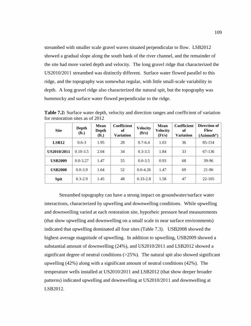
109

streambed with smaller scale gravel waves situated perpendicular to flow. LSB2012

showed a gradual slope along the south bank of the river channel, and the remainder of

the site had more varied depth and velocity. The long gravel ridge that characterized the

US2010/2011 streambed was distinctly different. Surface water flowed parallel to this

ridge, and the topography was somewhat regular, with little small-scale variability in

depth. A long gravel ridge also characterized the natural spit, but the topography was

hummocky and surface water flowed perpendicular to the ridge.

Table 7.2: Surface water depth, velocity and direction ranges and coefficient of variation

for restoration sites as of 2012

Site Depth

(ft.)

Mean

Depth

(ft.)

Coefficient

of

Variation

Velocity

(ft/s)

Mean

Velocity

(Ft/s)

Coefficient

of

Variation

Direction of

Flow

(Azimuth)

LSB12 0.6-3 1.95 28 0.7-6.4 1.03 36 85-154

US2010/2011 0.10-3.5 2.04 34 0.3-3.5 1.84 33 67-136

USB2009 0.0-3.27 1.47 55 0.0-3.5 0.93 68 39-96

USB2008 0.0-3.9 1.64 52 0.0-4.26 1.47 69 21-96

Spit 0.3-2.9 1.45 48 0.33-2.8 1.58 47 22-105

Streambed topography can have a strong impact on groundwater/surface water

interactions, characterized by upwelling and downwelling conditions. While upwelling

and downwelling varied at each restoration site, hyporheic pressure head measurements

(that show upwelling and downwelling on a small scale in near surface environments)

indicated that upwelling dominated all four sites (Table 7.3). USB2008 showed the

highest average magnitude of upwelling. In addition to upwelling, USB2009 showed a

substantial amount of downwelling (24%), and US2010/2011 and LSB2012 showed a

significant degree of neutral conditions (>25%). The natural spit also showed significant

upwelling (42%) along with a significant amount of neutral conditions (42%). The

temperature wells installed at US2010/2011 and LSB2012 (that show deeper broader

patterns) indicated upwelling and downwelling at US2010/2011 and downwelling at

LSB2012.

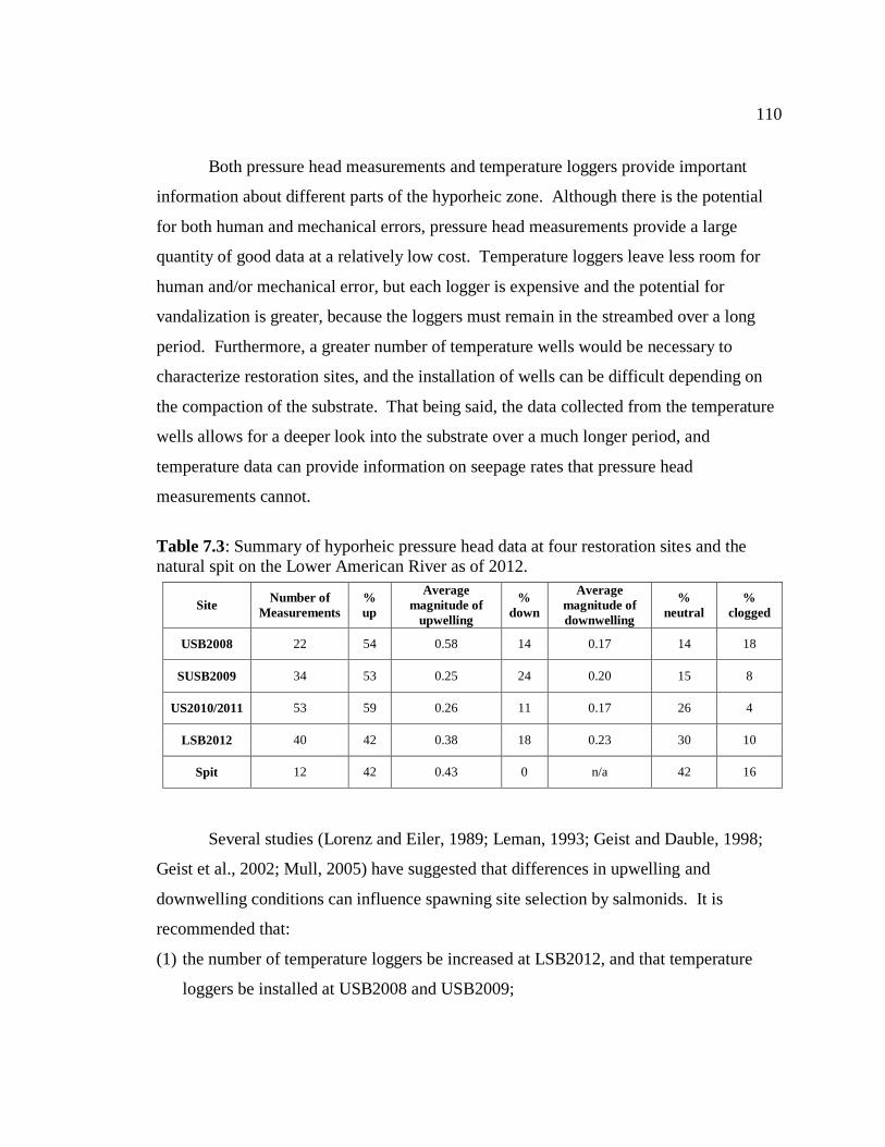
110

Both pressure head measurements and temperature loggers provide important

information about different parts of the hyporheic zone. Although there is the potential

for both human and mechanical errors, pressure head measurements provide a large

quantity of good data at a relatively low cost. Temperature loggers leave less room for

human and/or mechanical error, but each logger is expensive and the potential for

vandalization is greater, because the loggers must remain in the streambed over a long

period. Furthermore, a greater number of temperature wells would be necessary to

characterize restoration sites, and the installation of wells can be difficult depending on

the compaction of the substrate. That being said, the data collected from the temperature

wells allows for a deeper look into the substrate over a much longer period, and

temperature data can provide information on seepage rates that pressure head

measurements cannot.

Table 7.3: Summary of hyporheic pressure head data at four restoration sites and the

natural spit on the Lower American River as of 2012.

Site Number of

Measurements

%

up

Average

magnitude of

upwelling

%

down

Average

magnitude of

downwelling

%

neutral

%

clogged

USB2008 22 54 0.58 14 0.17 14 18

SUSB2009 34 53 0.25 24 0.20 15 8

US2010/2011 53 59 0.26 11 0.17 26 4

LSB2012 40 42 0.38 18 0.23 30 10

Spit 12 42 0.43 0 n/a 42 16

Several studies (Lorenz and Eiler, 1989; Leman, 1993; Geist and Dauble, 1998;

Geist et al., 2002; Mull, 2005) have suggested that differences in upwelling and

downwelling conditions can influence spawning site selection by salmonids. It is

recommended that:

(1) the number of temperature loggers be increased at LSB2012, and that temperature

loggers be installed at USB2008 and USB2009;

111

(2) hyporheic pressure head data collection continue at all four sites, measurements be

collected at greater depths, and a higher density of measurements be collected in areas

showing higher redd density; and

(3) a thermal imaging camera be used to look for groundwater seeps that would indicate

upwelling at each of the sites.

As of 2012, D.O. levels at the four sites remained suitable for salmonid spawning.

In general, all sites presented low D.O. prior to restoration. Immediately after restoration,

D.O. levels significantly increased and showed less variability. In subsequent years, the

median D.O. levels for USB2008, USB2009 and US2010/2011 remained high, but the

range of values became more dispersed. Figure 7.2 is a box and whisker graph of percent

D.O. levels at each site over time. As of November 2012, the median D.O. levels for

USB2008, USB2009 and US2010/2011 were still much higher than the levels

immediately before restoration. However, the minimum D.O. values at these sites

decreased over time, and the range of values were more variable compared to levels

immediately following restoration.

The difference in variability at US2010/2011 between December 2011 and

November 2012 is considerable. While the median value changed from 84% saturation

in December 2011 to 90% saturation in November 2012, the minimum levels decreased

from 80% to 22% and the CV grew from 2 to 36. This data suggests that after the initial

increase in D.O. provided by gravel augmentation levels become more variable overtime.

Continued monitoring of the sites is essential to determine at what point D.O. will reach

pre-restoration levels.

112

0

10

20

30

40

50

60

70

80

90

100

110

DIs

solv

ed O

xyge

n (

% s

atu

rati

on

)

Before After Dec. Nov. Before After Dec. Nov. Before After Nov. Before After

2011 2012 2011 2012 2012 (Nov. 2012)

n=7 n=13 n=7 n=9 n=10 n=8 n=8 n=11 n=10 n=14 n=13 n=2 n=13

Upper Sailor Bar Upper Sailor Bar Upper Sunrise Lower Sailor Bar

2008 2009 2010/2011 2012


Figure 7.2: Box and whisker graph of dissolved oxygen levels (% saturation) over time

(before and after restoration) at all restoration sites.

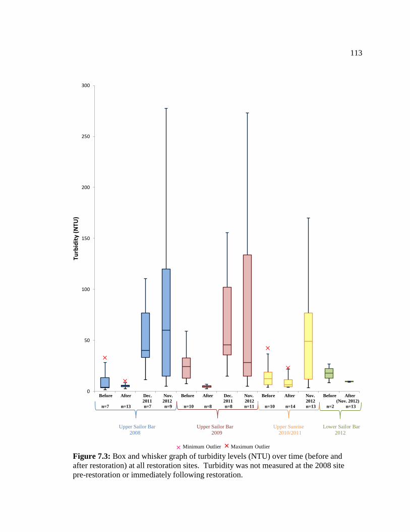
113

0

50

100

150

200

250

300

Turb

idit

y (N

TU)

Before After Dec. Nov. Before After Dec. Nov. Before After Nov. Before After

2011 2012 2011 2012 2012 (Nov. 2012)

n=7 n=13 n=7 n=9 n=10 n=8 n=8 n=11 n=10 n=14 n=13 n=2 n=13

Upper Sailor Bar Upper Sailor Bar Upper Sunrise Lower Sailor Bar

2008 2009 2010/2011 2012


Figure 7.3: Box and whisker graph of turbidity levels (NTU) over time (before and

after restoration) at all restoration sites. Turbidity was not measured at the 2008 site

pre-restoration or immediately following restoration.

114

Turbidity shows an increase with time at restoration sites. It is clear from Figure

7.3 that turbidity levels decreased immediately after gravel augmentation. This may be

due to screen washing before new gravel is added to the sites. However, in subsequent

years turbidity measurements became highly variable and many increased to levels well

above pre-restoration conditions. It is not clear if increases in intragravel turbidity levels

will affect salmonid spawning, because salmonids move gravel when constructing a redd

and this process may reduce the amount of sediment in completed redds. Future data

collection at the restored sites will be critical for understanding how increases in turbidity

will affect spawning habitats over time.

Spawning Usage

Salmonid response to augmentation projects was observed over time by

examining the use of each restoration site during Fall-run Chinook salmon spawning

seasons. From 2007 to 2012, the U.S. Bureau of Reclamation used high-resolution aerial

images of the American River to estimate the number of redds at each restoration site and

the total number of redds for the entire river (Hannon, 2012) before augmentation,

immediately after augmentation, and during subsequent spawning seasons. Using this

data, we calculated the percent of total redds at restoration sites by dividing the number

of actual redds at each site by the total number of redds on the entire river. A summary

of this data is in Table 7.4.

All of the restoration sites showed an increase of redds during the spawning

season immediately following restoration. The two oldest sites (USB2008 and

USB2009) showed an increase in redds every year following restoration. Four years after

restoration, USB2008 had the highest number of redds seen at the site since 2007 (166 in

2012). Part of this is an overall population increase, but it is also a clear indication that

gravel augmentation is improving the spawning habitat for Chinook Salmon for at least

four years after restoration.

At first glance, USB2008 and USB2009 seem to show the greatest improvement

immediately after augmentation based on percent of total redds; USB2008 went from 0%

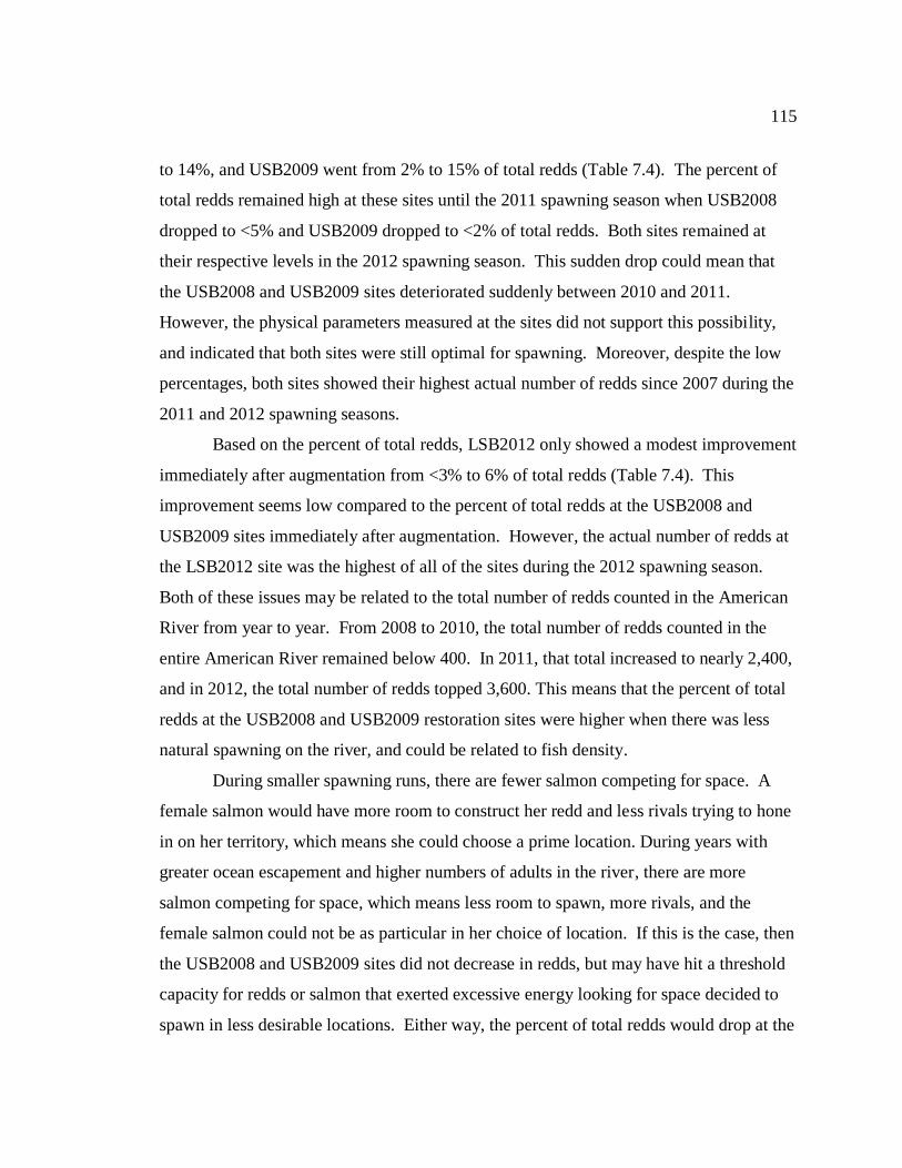
115

to 14%, and USB2009 went from 2% to 15% of total redds (Table 7.4). The percent of

total redds remained high at these sites until the 2011 spawning season when USB2008

dropped to <5% and USB2009 dropped to <2% of total redds. Both sites remained at

their respective levels in the 2012 spawning season. This sudden drop could mean that

the USB2008 and USB2009 sites deteriorated suddenly between 2010 and 2011.

However, the physical parameters measured at the sites did not support this possibility,

and indicated that both sites were still optimal for spawning. Moreover, despite the low

percentages, both sites showed their highest actual number of redds since 2007 during the

2011 and 2012 spawning seasons.

Based on the percent of total redds, LSB2012 only showed a modest improvement

immediately after augmentation from <3% to 6% of total redds (Table 7.4). This

improvement seems low compared to the percent of total redds at the USB2008 and

USB2009 sites immediately after augmentation. However, the actual number of redds at

the LSB2012 site was the highest of all of the sites during the 2012 spawning season.

Both of these issues may be related to the total number of redds counted in the American

River from year to year. From 2008 to 2010, the total number of redds counted in the

entire American River remained below 400. In 2011, that total increased to nearly 2,400,

and in 2012, the total number of redds topped 3,600. This means that the percent of total

redds at the USB2008 and USB2009 restoration sites were higher when there was less

natural spawning on the river, and could be related to fish density.

During smaller spawning runs, there are fewer salmon competing for space. A

female salmon would have more room to construct her redd and less rivals trying to hone

in on her territory, which means she could choose a prime location. During years with

greater ocean escapement and higher numbers of adults in the river, there are more

salmon competing for space, which means less room to spawn, more rivals, and the

female salmon could not be as particular in her choice of location. If this is the case, then

the USB2008 and USB2009 sites did not decrease in redds, but may have hit a threshold

capacity for redds or salmon that exerted excessive energy looking for space decided to

spawn in less desirable locations. Either way, the percent of total redds would drop at the

116

restoration sites, but not because of reduced habitat conditions or lower spawning usage.

This would also mean that the improvement at the LSB2012 site immediately after

augmentation was much greater than the percent of total redds indicated. This distinct

improvement is particularly evident in the locations of redds from year to year at

LSB2012 as seen in Figure 7.4. In 2011 (before restoration), the majority of redds were

located near the upstream portion of the south bank of the river. In 2012 (after

restoration), redds were distributed throughout the entire site.

Table 7.4: Redd counts on the Lower American River from 2007 to 2012 (Hannon, 2012)

Site Photo Date

Total Redds

in the River

Redds per

Site

% of Total

Redds

USB2008

11/27/2007 Before 839 0 0.00%

12/1/2008 Immediately after 312 43 13.78%

12/1/2009 1 year after 145 48 33.10%

11/11/2010 2 years after 359 66 18.38%

11/21/2011 3 years after 2394 116 4.85%

11/26/2012 4 years after 3619 166 4.59%

USB2009

11/12/2008 Before 239 5 2.09%


11/11/2010 1 year after 359 42 11.70%

11/21/2011 2 years after 2394 46 1.92%

11/26/2012 3 years after 3619 63 1.74%

US2010/2011

12/1/2009 Before 145 2 1.38%


11/26/2012 1 year after 3619 6 0.17%

LSB2012 11/21/2011 Before 2394 64 2.67%


Redd counts are inexact, because redds can be built over one another, it is difficult to

distinguish the number of individual redds in a group, and reflections and shadows make

counting redds from photos challenging.

It is also clear that the US2010/2011 site is receiving particularly low usage

compared to the other sites regardless of the total number of redds on the river. This is

the only site to see a decrease in the number of redds during any of the years following

restoration (Table 7.4). While the individual parameters measured in this study show

optimal conditions for salmonid spawning at US2010/2011, it is still unclear why the

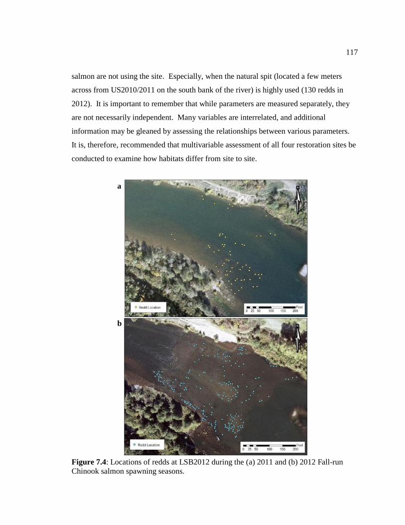
117

salmon are not using the site. Especially, when the natural spit (located a few meters

across from US2010/2011 on the south bank of the river) is highly used (130 redds in

2012). It is important to remember that while parameters are measured separately, they

are not necessarily independent. Many variables are interrelated, and additional

information may be gleaned by assessing the relationships between various parameters.

It is, therefore, recommended that multivariable assessment of all four restoration sites be

conducted to examine how habitats differ from site to site.

a

b

Figure 7.4: Locations of redds at LSB2012 during the (a) 2011 and (b) 2012 Fall-run

Chinook salmon spawning seasons.

118

Summary of Recommendations

Gravel augmentation projects on the Lower American River are improving

salmonid spawning habitats. Immediately following restoration, physical parameters

measured in this study showed significant improvement when compared to pre-

restoration conditions. Over time, these sites are continuing to provide optimal

conditions for salmonid spawning, but the sites are changing and showing signs of an

eventual return to pre-restoration conditions. The longevity of these restoration projects

is still unclear, and further monitoring is necessary to establish the duration of habitat

improvement. Furthermore, redd counts are showing that usage of the sites by spawning

salmonids varies. To understand why salmon are choosing one site over another, it is

important to continue monitoring sites and identify variables that predict fish use or good

habitat. The following is a summary of recommendations outlined in this report:

(1) Conduct three to five bulk samples at each site within the next year to quantify

current surface and subsurface grain size and evaluate streambed armoring.

(2) Dig out missing scour chains during the next low flow event to determine if

deposition or erosion is occurring.

(3) Replace missing scour chains at the USB2009, US2010/2011, and LSB2012 sites

and install new scour chains at the USB2008 site.

(4) Use a total station to survey each site within the next year to determine current

streambed topography and evaluate how restoration sites have morphed over time.

(5) Consider ending the use of tracer rocks for analyzing gravel mobility.

(6) Conduct higher density permeability measurements at all sites.

(7) Continue monitoring water quality of all sites to determine at what point

parameters (D.O. and turbidity) will reach pre-restoration levels.

(8) Conduct higher density grain size analysis, depth and velocity, temperature, and

hyporheic pressure head measurements in zones with high use by spawning

salmonids.

(9) Conduct hyporheic pressure head measurements at greater depths at all sites.

(10) Implement the use of a thermal imaging camera to find groundwater seeps.

119

(11) Continue monitoring temperature at the US2010/2011 site and adjacent natural

spit, install temperature loggers at the USB2008 and USB2009 sites, and increase

the number of loggers the LSB2012 site.

(12) Conduct multivariable assessment of all four restoration sites to examine the

interrelation or physical variables and how habitats differ from site to site.

120

8.0 REFERENCES

Barnard, K. and McBain, S., 1994, Using a Standpipe to Determine Permeability,

Dissolved Oxygen, and Vertical Particle Size Distribution in Salmonid Spawning

Gravels. As FHR Currents # 15, US Forest Service, Region 5. Eureka, CA. 12 pp.

Bash. J., Berman. C., and Folton. S., 2001, Effects of Turbidity and Suspended Solids on

Salmonids. Center of Streamside Studies. University of Washington.

Becker, C.D., Neitzel, D.A. and Abernethy, C.S, 1983, Effects of dewatering on Chinook

salmon redds: tolerance of four developmental phases to one-time dewatering.

North American Journal of Fisheries Management 3:373-382.

Bencala E., 2005, Hyporheic exchange flows. In: Anderson MG and McDonnell JJ (Eds),

Encyclopedia of Hydrological Sciences. John Wiley and Sons, London, v 3, p.

1733-1740.

Bigelow, P., 2005, Testing and improving predictions of scour and fill depths in a

northern California coastal stream. River Research and Applications. 21, p. 909-

923.

Bjornn, T.C., and Reiser, D.W., 1991, Habitat requirements of salmonids in streams,

American Fisheries Society Special Publication 19: p. 83-138. (Note: This

publication is Chapter 4 in Influences of forest and rangeland management on

salmonid fishes and their habitats [W.R. Meechan, editor].)

Boggs, S., 2011, Principles of Sedimentology and Stratigraphy, Fifth edition, Upper

Saddle River, N.J., Pearson Prentice Hall.

BOR, 2012, The American River Gravel Project: Project Photos:

http://www.usbr.gov/mp/PA/gravel.html, accessed April 2013.

Bunte, K. and Abt, S.R., 2001, Sampling surface and subsurface paricle-size

distributions in wadable gravel- and cobble-bed streams for analyses in sediment

transport, hydraulics, and streambed monitoring. United States Department of

Agricultural. Rocky Mountain Research Station.

Bush, N.J., 2006, Natural water chemistry and vertical hydraulic gradient in the

hyporheic zone of the Cosumnes River near Sacramento, CA. M.S. thesis. CSUS.

Carling, P. A., McCahon, C. P., 1987, Natural siltation of brown trout (salmo trutta L.)

spawning gravels during low-flow conditions, Regulated Streams, Advances in

Ecology, ed. By Craig, J. F., and Kemper, J. B., p. 229-244, Plenum Press, New

York.

121

Chapman, D.W., Weitkamp, D.E., Welsh, T.L., Bell, M.B. and Schadt, T.H., 1986,

Effects of riverflow on the distribution of Chinook salmon redds: Transactions of

the American Fisheries Society, v.115, p. 537-547.

Chevalier, B.C., Carson, C., and Miller, W. J., 1984, Report of engineering and biological

literature pertaining to the aquatic environment: with special emphasis on

dissolved oxygen and sediment effects on salmonid habitat, Colorado State

University, Department of Agriculture and Chemical Engineering, ARS Project

5602-2081 3-008A, Fort Collins.

Coble, D. W., 1961, Influence of water exchange and dissolved oxygen inredds on

survival of steelhead trout embryos, Transactions of the American Fisheries

Society, v. 90, p. 469-474.

Compton, R. R., 1962, Geology in the Field, New York, John Wiley and Sons, Inc.

Cordone, A. J. and Kelley, D. W., 1961, The influences of inorganic sediment on the

aquatic life of streams, Reprint from California Fish and Game, V. 47, N. 2.

California Department of Fish and Game, Inland Fisheries Branch, Sacramento,

CA.

Davis, J.C., 1975, Minimal dissolved oxygen requirements of aquatic life with emphasis

on Canadian species: a review. Journal of Fisheries Research Board Canada.

32(12), 2295-2332.

Devries, P.E., 2000, Scour in low graidient gravel bed stream: Patterns, processes and

implications for the salmonid embryos. Ph.D. Thesis. University of Washington:

United States.

DeVries, P., 1997, Riverine salmonid egg burial depths: review of published data and

implications for scour studies, Can. J. Fish. Aquatic Science v. 54, p. 1685-1698.

Ettema, R., 1984, Sampling armor-layer sediments. Journal of Hydraulics Division. v.

110. 7 p. 992–996.

Fairman, D., 2007, A gravel budget for the Lower American River. M.S. thesis. CSUS.

Fetter, C.W., 2001, Applied Hydrogeology: New York, NY, Macmillan College

Publishing Company, p. 598.

Folk, R. L. and Ward, W. C., 1957, Brazos River bar: a study in the significance of grain

size parameters, Journal of Sedimentary Petrology, v. 27, p. 3–26.

122

FSC: Field Studies Council, 2012, Life in Freshwater: Channels:

http://www.lifeinfreshwater.org.uk/Web%20pages/Rivers/Channels.htm, accessed

April 2013.

Geist D. R. and Dauble, D. D., 1998, Redd site selection and spawning habitat use by fall

Chinook salmon: The importance of geomorphic features in large rivers:

Environmental Management, v. 22, p. 655-669.

Geist, D. R., Hanrahan, T. P., Arntzen, E. V., McMichael, G. A., Murray, C. J., Chien,

Y., 2002, Physicochemical Characteristics of the Hyporheic Zone Affect Redd

Site Selection by Chum Salmon and Fall Chinook Salmon in the Columbia River,

North American Journal of Fisheries Management, v. 22, p. 1077-1085.

Greig, S.M., Sear, D.A. and Carling, P.A., 2007, Review of factors influencing the

availability of dissolved oxygen to incubating salmon embryos. Hydrological

Processes. v. 21. p. 323-334.

Hannon, J. and Deason, B., 2005, American River Steelhead (Onchorhynchus Mykiss)

Spawning 2001 - 2005. Central Valley Project, American River, California Mid-

Pacific Region. United States Bureau of Reclamation.

Hannon, J., 2000, Personal communication on Steelhead spawning parameters.

Hannon, J., 2012, United States Bureau of Reclamation: American River Chinook Redd

Counts from aerial photos.

Harvey, B., Lisle, T., 1999, Scour of Chinook Salmon Redds and Suction Dredge

Tailings. North American Jornal of Fisheries Management.

Haschenburger, J. K., 1999, A probability model of scour and fill depths in gravel-bed

channels. Water Resources Research. 35, #9, p. 2857-2869.

Henley. W., Patterson, M. Neves. R., Lemly. D., 2000, Effects of Sedimentation and

Turbidity on Lotic Food Webs: A Concise Review for Natural Resource

Managers. Fisheries Science. v. 8 2. p. 125-139.

Horner, T. C., Titus R., Brown M., 2004, Phase 3 Gravel Assessment on the Lower

American River: Report to the U.S. Bureau of Reclamation Sacramento

Office. Unpublished report,

Horner, T. C., 2005, Physical and geochemical characterization of American River

spawning gravels. Report to the U.S. Bureau of Reclamation Sacramento Office.

Unpublished report,

123

Horner, T. C., 2005, 2005 report to the Sacramento Water Forum: Site Assessment at the

Lower Sunrise Side Channel: Surface Water, Pore Water and Intergravel

Flow. Unpublished report.

Horner, T. C., 2010, Physical and geochemical characteristics of the 2009 Sailor Bar

gravel addition, Unpublished report to the U.S. Bureau of Reclamation,

Sacramento office, 77 p.

Ingebritsen, S. E., and Sanford, W. E., 1998, Groundwater in Geologic Processes.

Cambridge, UK: Cambridge University Press.

Inman, D. L., 1952, Measures for describing the size distribution of sediments, Journal of

Sedimentary Petrology, V. 22, p. 125–145.

Janes, M. K., Heffernan, J., Rosenberry, J., Adrian, J. and Novotny, N., 2012, Physical

and geochemical characteristics of the Upper Sailor Bar 2008, Upper Sailor Bar

2009 and Upper Sunrise 2010/2011 gravel additions, ed. by Horner, T. C.,

unpublished report to the U.S. Bureau of Reclamation, Sacramento office, 105 p.

Jones, J. B., and Mulholland, P. J., 2000, Streams and ground waters: San Diego,

Academic Press.

Kondolf, G. M., 1997, Application of the pebble count: reflections on purpose, method,

and variants. Water Resources Bulletin 33:79-87.

Kondolf. G. M., 2000, Assessing Salmonid Spawning Gravel Quality. Transactions of the

American Fisheries Society. v. 129. 1.

Kondolf, G. M., Williams, J.G., Horner, T.C., Milan, D., 2008, Assessing Physical

Quality of Spawning Habitat. American Fisheries Society Symposium. 65

Leman, V. N., 1993, Spawning sites of chum salmon, Oncorhynchus kets:

Microhydrological regime and viability of progeny in redds (Kamchatka River

Basin), Journal of Ichthyology, V. 33, p. 104-117.

Leopold, L. B., Wolman, M. G. and Miller, J. P., 1964, Fluvial processes in

geomorphology. Freeman, San Francisco.

Leopold, L. B., 1970, An Improved Method for Size Distribution of Stream Bed Gravel,

Water Resources Research, v. 6, is. 5, p. 1357-1366.

Lisle, T. E. and Eads, R. E., 1991, Methods to measure sedimentation of spawning

gravels. USDA For. Serv. Res. Note PSW-411. Pacific Southwest Res. Stat.

Berkeley.

124

Lorenz, J. M., and Eiler, J. H., 1989, Spawning habitat and redd characteristics of

sockeye salmon in the glacial Taku River, British Columbia and Alaska,

Transactions of the American Fisheries Society V. 118, p. 495–502.

Madej, M. A., 1984, Recent changes in channel-stored sediment Redwood Creek,

California. Redwood National Park Research and Development Technical Report

11, National Park Service, Arcata, CA, 54 p.

Malcolm. I., Youngson. A., Soulsby. C., 2003, Survival of salmonid eggs in a degraded

gravel-bed stream: effects of groundwater–surface water interactions. River

Research and Applications. v. 19. 4. p. 303-316.

McNeil, W. H., 1966, Effect of the spawning bed environment on reproduction of pink

and chum salmon, Fishery Bulletin Volume 65, Number 2, Contribution Number

198, College of Fisheries, University of Washington, Seattle.

Merz, J. E. and Setka, J. D., 2004, Evaluation of a spawning habitat enhancement site for

Chinook salmon in a regulated California river, North American Journal of

Fisheries Management, v. 24, p. 397-407.

Monaghan, K. A. and Milner, A. M., 2009, The effect of anadromous salmon redd

construction on macroinvertebrate communities in a recently formed stream in

coastal Alaska, Journal of the North American Benthological Association, V. 28,

p. 153-166.

Mull, K. E., 2005, Selection of spawning sites by coho salmon (O. kisutch) in Freshwater

Creek, California, MS, Thesis, Humboldt St. University, CA.

Nawa, R.K., Frissell, C.A., 1993, Measuring scour and fill of gravel streambeds with

scour chains and sliding-bead monitors. North American Journal of Fisheries

Management. 12, 634-639.

Nawa, R. K., Frissell, C. A. and Liss, W. J., 1990, Life history and persistence of

anadromous salmonid stocks in relation to stream habitats and watershed

classification, Annual progress report: Fish Research Project, Oregon, Department

of Fisheries and Wildlife, Oregon State University, Corvallis.

Neville, A.M. and Kennedy, J.B., 1964, Basic Statistical Methods for Engineers and

Scientists, International Textbook Company, Scranton, Pennsylvania, pg. 33

Phillips, J. D., 2003, Toledo Bend Reservoir and geomorphic response in the lower

Sabine River, River Research and Applications, v. 19, p. 137-159.

125

Redd, R. and Horner, T. C., 2009, Physical and geochemical characteristics of the Lower

Sunrise side channel restoration project, Submitted to the Sacramento Water

Forum.

Redd, R. and Horner, T. C., 2010, Physical and geochemical characteristics of the 2009

Sailor Bar gravel addition, Unpublished M.S. thesis, CSUS library.

Seegrist, D.W. and Gard, R., 1972, Effects of floods on trout in Sagehen Creek,

California, Transactions of the American Fisheries Society v. 101, p. 478-482.

Shlemon, R. J., 1967a, Landform-soil Relationships in Northern Sacramento County,

California: Ph.D. dissertation, U.C. Berkeley, Department of Geography, 295 p.

plus map and cross sections.

Snider, B., Christophel, D.B., Jackson, B.L., and Bratovitch, P.M., 1992, Habitat

characterization of the Lower American River, California Department of Fish and

Game, Environmental Services Division in cooperation with Beak Consultants

and the county of Sacramento, California, Unpublished report, 20 p.

Soulsby. C., Youngson. A., Moir. H., Malcolm. I., 2001, Fine Sediment influence on

salmonid spawning habitat in a lowland agricultural stream: preliminary

assessment. Scienc of Total Environment. v. 263. p. 295-307.

Stonestrom, D.A., and Constantz, J., eds., 2003, Heat as a Tool for Studying the

Movement of Ground Water Near Streams: U.S. Geological Survey Circula, p.

1260, 96.

Storey, R. G., Howard, K. W. F., and Williams, D. D., 2003, Factors controlling riffle-

scale hyporheic exchange flows and their seasonal changes in a gaining stream A

three-dimensional groundwater flow model, Water Resources Research, v. 39, no.

2, 1034.

Suttle, K. B., Power, M. E., Levine, J. M., and McNeely, C., 2004, How fine sediment in

riverbeds impairs growth and survival of juvenile salmonids, Ecological

Applications 14(4): 969-974.

Terhune, L. D. B., 1958, The Mark VI groundwater standpipe for measuring seepage

through salmon spawning gravel, Journal of the Fisheries Research Board of

Canada, V. 15, 1027–1063.

Tripp, D. B., and Poulin, V. A., 1986, The effects of logging and mass wasting on

salmonid spawning habitat in streams on the Queen Charlotte Islands, Land

Manage, Report 50, B.C. Min. For. Lands, Victoria, B.C.

126

Tucker, M. E., 1996, Sedimentary rocks in the field, John Wiley and Sons, Chichester,

153 p.

Hyporheic Network, 2009, The hyporheic handbook, a handbook on the groundwater-

surface water interface and hyporheic zone for environment managers. Environment Agency R&D Publication 95. EA, Bristol.

USGS, 1980, General Procedure for Gaging Streams: Techniques of Water-Resources

Investigations of the United States Geological Survey, U.S. Department of

Interior, Office of Water Data Coordination, U.S. Geological Survey.

USGS, 2013, USGS Real-Time Water Data for the Nation:

http://waterdata.usgs.gov/usa/nwis/uv?site_no=11446500 (Accessed July 2013).

Vanoni, V. A. and Brooks, N. H., 1957, Laboratory studies of the roughness and

suspended load of alluvial streams, Sedimentation Laboratory, California Institute

of Technology, Pasadena, California.

Vronskiy, B. B., and, Leman, V. N., 1991, Spawning stations, hydrological regime, and

survival of progeny in nests of chinook salmon,Oncorhynchus tshawytscha,in the

Kamchatka River Basin, Voprosy Ikhtiologii V. 31, 282–291.

Williams, J., 1999, Chinook salmon in the Lower American River California’s largest

urban stream: Fish Bulletin 179: volume 2.

Woessner, W. W., 2000, Stream and fluvial plain ground water interactions: Rescaling

hydrogeologic thought, Groundwater, v. 38, p. 423-429.

Wolman. M., 1954, A method of sampling coarse river-bed material. Transactionsm

American Geophysical Union. V. 35, 6.

Wu, F., 2000, Modeling Embryo Survival affected by sediment deposition into salmonid

spawning gravels: Water Resources Research, v. 36, pp. 1595- 1603.

UCLA, 2013, What is the coefficient of variation? UCLA: Statistical Consulting Group:

http://www.ats.ucla.edu/stat/mult_pkg/faq/general/coefficient_of_variation.htm

(accessed July 2, 2013).

Vaux, W. G., 1962, Intragravel Flow and Interchange of Water in a Streambed, Fishery

Bulletin, v. 66, no. 3, p. 479-489.

127

Vyverberg , K., Snider, B., and Titus, R.G., 1997, Lower American River

ChinookSalmon Spawning Habitat Evaluation October 1994: California

Department of Fish andGame Environmental Services Division. Technical Report

No. 97-2, p. 112.

Youngson, A., Malcolm, I., Thorley, J., Bacon, P., Soulsby, C., 2004, Long-residence

groundwater effects on incubating salmonid eggs: low hyporeic oxygen impairs

embryo development. Canadian Journal of Fisheries and Aquatic Sciences. V. 61.

12

Zamora, C., 2006, Estimating rates of exchange across the sediment/water interface in the

Lower Merced River, CA. M.S. thesis, CSUS library, p. 102.

Documents

Physical and geochemical characteristics of the Lower Sailor Bar 2012 ... bean 2012 gravel... · Physical and geochemical characteristics of the Lower Sailor Bar 2012, Upper Sunrise