Embed Size (px)
Citation preview

Physical modeling and numerical studies of three-dimensional non-equilibriummulti-temperature flowsGuiyu Cao (曹贵瑜), Hualin Liu (刘华林), and Kun Xu (徐昆)
Citation: Physics of Fluids 30, 126104 (2018); doi: 10.1063/1.5065455View online: https://doi.org/10.1063/1.5065455View Table of Contents: http://aip.scitation.org/toc/phf/30/12Published by the American Institute of Physics
Articles you may be interested inThe three-dimensional impulse response of a boundary layer to different types of wall excitationPhysics of Fluids 30, 124103 (2018); 10.1063/1.5063700
Transient evolution of the heat transfer and the vapor film thickness at the drop impact in the regime of filmboilingPhysics of Fluids 30, 122109 (2018); 10.1063/1.5059388
Investigations of data-driven closure for subgrid-scale stress in large-eddy simulationPhysics of Fluids 30, 125101 (2018); 10.1063/1.5054835
Generalised Navier boundary condition for a volume of fluid approach using a finite-volume methodPhysics of Fluids 31, 021203 (2019); 10.1063/1.5055036
A numerical study of oscillation induced coalescence in bubbly flowsPhysics of Fluids 30, 127105 (2018); 10.1063/1.5059558
Investigation of near-wall turbulence in relation to polymer rheologyPhysics of Fluids 30, 125111 (2018); 10.1063/1.5062156

PHYSICS OF FLUIDS 30, 126104 (2018)
Physical modeling and numerical studies of three-dimensionalnon-equilibrium multi-temperature flows
Guiyu Cao (曹贵瑜),1,a) Hualin Liu (刘华林),2,b) and Kun Xu (徐昆)1,3,c)1Department of Mathematics, Hong Kong University of Science and Technology, Clear Water Bay,Kowloon, Hong Kong2College of Aeronautics and Astronautics, Zhejiang University, Hangzhou, Zhejiang 310058, China3Department of Mechanical and Aerospace Engineering, Hong Kong University of Science and Technology,Clear Water Bay, Kowloon, Hong Kong
(Received 10 October 2018; accepted 29 November 2018; published online 28 December 2018)
For increasingly non-equilibrium flowfields, the Navier-Stokes equations lose accuracy partially dueto the single temperature approximation. To overcome this barrier, a continuum multi-temperaturemodel based on the Bhatnagar-Gross-Krook equation coupled with the Landau-Teller-Jeans relax-ation model has been proposed for two-dimensional hypersonic non-equilibrium multi-temperatureflow computation. In a recent study, a two-stage fourth-order gas-kinetic scheme (GKS) has beendeveloped for equilibrium flows, which achieves a fourth-order accuracy in space and time as wellas high efficiency and robustness. In this paper, targeting for accurate and efficient simulation ofmulti-temperature non-equilibrium flows, a high-order three-dimensional multi-temperature GKS isconstructed under the two-stage fourth-order framework, with the fourth-order Simpson interpolationrule for the newly emerged source term. Simulations on decaying homogeneous isotropic turbulence,low-density nozzle flow, rarefied hypersonic flow over a flat plate, and type IV shock-shock inter-action are used to validate the multi-temperature model through the comparison with experimentalmeasurements. The unified gas kinetic scheme (UGKS) results and the Direct Simulation Monte Carlo(DSMC) solutions will be used as well in some cases for validation. Computational results not onlyconfirm the high-order accuracy and quite robustness of this scheme but also show the significantimprovement on computational efficiency compared with UGKS and DSMC, especially for the flowin the near continuum regime. Published by AIP Publishing. https://doi.org/10.1063/1.5065455
I. INTRODUCTION
The classification of flow regimes is based on the Knud-sen number Kn, which is defined as the ratio of the molecularmean free path over a characteristic length scale of the system.The whole flow regime is roughly divided into the contin-uum flow regime (Kn ≤ 0.001), continuum-transition regime(0.001 < Kn ≤ 10), and free molecular regime (Kn > 10). TheNavier-Stokes (NS) equations with linear relations betweenstress and strain and Fourier’s laws are adequate to modelthe equilibrium flow in the continuum flow regime. For thenon-equilibrium flow in the continuum-transition regime, theNavier-Stokes equations are well known to be inadequate.However, this continuum-transition regime is important formany scientific and practical engineering applications such asthe simulation of micro-scale flows and space exploration vehi-cles.1 Therefore, accurate models with reliable solutions andlower computational costs for non-equilibrium flow are use-ful for solving the non-equilibrium flow problem in the nearcontinuum regime.
Available numerical schemes for simulating non-equilibrium flow can be classified into the particle methodand deterministic method. Direct simulation Monte Carlo
a)Electronic mail: [email protected])Electronic mail: [email protected])Electronic mail: [email protected]
(DSMC)2 uses probabilistic simulation to solve the Boltz-mann equation, which is a representative of the particle methodand is widely used for rarefied flow simulations. However,in the continuum-transition regime, DSMC requires a greatamount of particles and the cell size and time step are lim-ited by the particle mean free path and mean collision time,and it becomes very expensive both in the memory cost andcomputational time. The deterministic methods, such as Dis-crete Velocity Methods (DVMs) or Discrete Ordinate Meth-ods (DOMs)3–5 which adopt splitting treatment of free trans-port and collision, solve the Boltzmann or model equationsdirectly with the discretization of particle velocity space. Inthe continuum-transition regime, the cell size and time stepare also constrained by the particle mean free path and meancollision time, which make these methods prohibitively expen-sive. Recently, an improved DVM6 is proposed to use a largetime step and cell size by coupling the transport and colli-sion in a hybrid flux, where the collisionless flux is computedby the discrete velocity distribution function and the colli-sional hydrodynamic flux is computed by the NS solver. Themulti-scale unified gas kinetic scheme (UGKS)7–10 has beendeveloped successfully for monatomic and diatomic gases forthe entire Knudsen number flow. Different from the splittingprocess used in DSMC and DVM/DOM methods, the distin-guishable feature of UGKS is the coupling of the particletransport and collision, which makes the grid size and timestep used in UGKS not limited by the particle mean free path
1070-6631/2018/30(12)/126104/15/$30.00 30, 126104-1 Published by AIP Publishing.
126104-2 Cao, Liu, and Xu Phys. Fluids 30, 126104 (2018)
and collision time. Even though UGKS is currently the mostefficient DVM-type multiscale method for flow simulation inthe whole flow regime, in view of a considerable number ofdiscrete velocity points to be updated, it is still expensive in thenear continuum flow regime than those based on the macro-scopic equations. At the same time, for smooth flow, such asthose in the boundary layer, a high-order scheme is preferredto get accurate solutions. However, most schemes for the rar-efied flow, such as DSMC, DVM/DOM, and UGKS, have onlyat most second-order accuracy.
To study non-equilibrium flow efficiently, an extendedBhatnagar-Gross-Krook (BGK) model coupled with theLandau-Teller-Jeans relaxation model has been proposed forone-dimensional and two-dimensional non-equilibrium multi-temperature flow computation.11,12 In the continuum flowregime, the corresponding kinetic scheme goes back auto-matically to the BGK-NS method. On the other hand, thiskinetic scheme solves the non-equilibrium translational androtational flow quite efficiently in the near continuum regime.In recent studies, an accurate and robust two-stage fourth-order gas-kinetic scheme (GKS)13,14 has been developed forequilibrium flows, which achieves a fourth-order accuracy inspace and time, and shows high efficiency and robustnessfrom the smooth flow to shock problem. In order to capturethe delicate flow structure, a high-order non-equilibrium GKSbased on the extended BGK method is preferred for simu-lating the multi-temperature flow efficiently and accurately.In the current study, this high-order non-equilibrium GKS isimplemented under the previous two-stage fourth-order frame-work for three-dimensional multi-temperature flows, and thesource term is dealt with by the fourth-order Simpson inter-polation rule. Numerical tests from smooth decaying homoge-neous isotropic turbulence to challenging hypersonic type IVshock-shock interaction validate the current high-order non-equilibrium GKS. This high-order non-equilibrium GKS notonly preserves high accuracy and quite robustness throughnumerical cases but also shows the significant improve-ment on computational efficiency in the near continuum flowregion.
In this paper, details on the current extended kinetic modeland corresponding macroscopic equations are presented inSec. II. Section III gives the construction of this high-ordernon-equilibrium numerical scheme under a two-stage fourth-order framework for solving this extended kinetic model. Thisis followed by the results and discussion of the non-equilibriummulti-temperature flow computations in Sec. IV. Discussionand conclusion are shown in Sec. V.
II. GAS-KINETIC MODELS AND MACROSCOPICGOVERNING EQUATIONS FOR DIATOMIC GAS
In this section, the extended kinetic model and its derivedmacroscopic equations in three dimensions for diatomic gasesare presented.
A. Equilibrium translational and rotationaltemperature model
By modeling the time evolution of a gas distributionfunction resulting from the free transport and binary elastic
collision, the Boltzmann equation has been constructed formonotonic dilute gas. The simplification of the Boltzmannequation given by the BGK model has the following form:15
∂f∂t
+ u∂f∂x
+ v∂f∂y
+ w∂f∂z=
g − fτ
, (1)
where f is the number density of molecules at the position(x, y, z) and particle velocity (u, v , w) at time t. The left-hand side of Eq. (1) denotes the free transport, and the right-hand side represents the collision term. The relation betweenthe distribution function f and macroscopic variables, such asmass, momentum, energy, and stress, can be obtained by takingmoments of the distribution function. The collision operatorin the BGK model shows a simple relaxation process from fto a local equilibrium state g, with a characteristic time scale τrelated to the viscosity and heat conduction coefficients. Thelocal equilibrium state is a Maxwellian distribution,
g = ρ(λ
π)
K+32 e−λ[(u−U)2+(v−V )2+(w−W )2+ξ2], (2)
where ρ is the density, (U, V, W ) are the macroscopic fluidvelocities in the x-, y-, and z- directions. Here λ = m/2kT,where m is the molecular mass, k is the Boltzmann constant,and T is the temperature. For three-dimensional equilibriumdiatomic gas, the total number of degrees of freedom K = 2,the internal variable ξ accounts for the rotational modes asξ2 = ξ2
1 + ξ22 , and the specific heat ratio γ = (K + 5)/(K + 3) is
determined.Based on the above BGK model as Eq. (1), the Euler
equations can be obtained for a local equilibrium state withf = g. On the other hand, for the Navier-Stokes equations, thestress and Fourier heat conduction terms can be derived withthe Chapman-Enskog expansion16 truncated to the 1st-order,
f = g + Knf1 = g − τ(∂g∂t
+ u∂g∂x
+ v∂g∂y
+ w∂g∂z
). (3)
For the Burnett and super-Burnett equations, the above expan-sion can be naturally extended,17 such as f = g + Knf 1 + Kn2f 2
+ Kn3f 3 + · · · . For the above Navier-Stokes solutions, the GKSbased on the kinetic BGK model has been well developed.18
In order to simulate the flow with any realistic Prandtl number,a modification of the heat flux in the energy transport is usedin GKS, which is also implemented in the present study.
B. Non-equilibrium translational and rotationaltemperature model
A single temperature is assumed for translational and rota-tional modes in the Navier-Stokes equations. However, it losesaccuracy in the simulation of the non-equilibrium flow becauseof the different temperatures for the translational and rota-tional energy modes. In this subsection, an extended BGKmodel for non-equilibrium rotational energy is constructedand for the first time, and the corresponding three-dimensionalmacroscopic governing equations are derived.
For the non-equilibrium multi-temperature diatomic gasflow, the above-mentioned BGK model can be extended in thefollowing form:
∂f∂t
+ u∂f∂x
+ v∂f∂y
+ w∂f∂z=
f eq − fτ
+g − f eq
Zrτ=
f eq − fτ
+ Qs,
(4)
126104-3 Cao, Liu, and Xu Phys. Fluids 30, 126104 (2018)
where an intermediate equilibrium state f eq is introduced withtwo temperatures, one for translational temperature and theother for rotational temperature,
f eq = ρ(λt
π)3/2(
λr
π)e−λt [(u−U)2+(v−V )2+(w−W )2]−λrξ
2r , (5)
where λt = m/2kT t is related to the translational tempera-ture T t and λr = m/2kT r accounts for the rotational tem-perature T r . Therefore, the right-hand side collision operatorcontains two terms corresponding to the elastic and inelasticcollisions, respectively, where the relaxation process becomesf → f eq → g and the inelastic collision process from f eq
to g takes a much longer time Zrτ than that of elastic colli-sion process by τ. The additional term Qs in the collision partaccounts for the energy exchange between the translational androtational energy, which contributes to the source term for thecorresponding three-dimensional macroscopic flow evolution.The above three-dimensional extended BGK model is a naturalextension for the two-dimensional extended BGK model.12
The relation between mass ρ, momentum (ρU, ρV, ρW ),total energy ρE, and rotational energy ρEr with the distributionfunction f is given by
W =
*........,
ρρUρVρWρEρEr
+////////-
=
∫ψαfdΞ, α = 1, 2, 3, 4, 5, 6, (6)
where dΞ = dudvdwdξr and ψα is the component of the vectorfor moments
ψ = (ψ1,ψ2,ψ3,ψ4,ψ5,ψ6)T
= (1, u, v , w,12
(u2 + v2 + w2 + ξ2r ),
12ξ2
r )T .
As a new temperature λr is introduced, the constraint ofrotational energy relaxation has to be imposed on the aboveextended kinetic model to self-consistently determine allunknowns. Since only mass, momentum, and total energyare conserved during particle collisions, the compatibilitycondition for the collision term turns into∫
(f eq − fτ
+ Qs)ψαdΞ = S = (0, 0, 0, 0, 0, s)T ,
α = 1, 2, 3, 4, 5, 6.(7)
The source term for the rotational energy is from the energyexchange between translational and rotational ones duringinelastic collision. The source term for the rotational energyis modeled through the Landau-Teller-Jeans-type relaxationmodel,
s =(ρEr)eq − ρEr
Zrτ. (8)
The equilibrium energy (ρEr)eq is determined by theassumption T r = T t = T such that
(ρEr)eq =ρ
2λeqr
and λeqr =
K + 34
ρ
ρE − 12 ρ(U2 + V2 + W2)
.
Here, the collision number Zr is related to the ratio of theelastic collision frequency to the inelastic frequency. The par-ticle collision time multiplied by a rotational collision numberZr models the relaxation process for the rotational energy toequilibrate with the translational one. The value Zr used in thecurrent study is as in the work of Parker,19
Zr =Z∞r
1 + (π3/2/2)√
T ∗/T + (π + π2/4)(T ∗/T ),
where the quantity T ∗ is the characteristic temperature ofintermolecular potential and Z∞r is the limiting value. Overa temperature range from 30 K to 3000 K for nitrogen, thevalues Z∞r = 23.0 and T ∗ = 91.5 K are used. The local temper-ature T in the above equation is the translational temperature.More advanced models for the energy relaxation are discussedin referred work.20
Using the intermediate state given by Eq. (5), with thefrozen of rotational energy exchange, the first-order Chapman-Enskog expansion gives
f = f eq +Knf1 = f eq−τ(∂f eq
∂t+u
∂f eq
∂x+v
∂f eq
∂y+w
∂f eq
∂z). (9)
The corresponding macroscopic non-equilibrium multi-temperature continuum equations in three-dimensions can bederived, as shown in the Appendix,
∂W∂t
+∂F∂x
+∂G∂y
+∂H∂z=∂Fv∂x
+∂Gv
∂y+∂Hv
∂z+ S, (10)
with
W =
*........,
ρρUρVρWρEρEr
+////////-
F =
*........,
ρUρU2 + pρUVρUW
(ρE + p)UρErU
+////////-
G =
*........,
ρVρUVρV2 + pρVW
(ρE + p)VρErV
+////////-
H =
*........,
ρWρUWρVW
ρW2 + p(ρE + p)WρErW
+////////-
,
and
Fv =
*........,
0τxx
τxy
τxz
Uτxx + Vτxy + Wτxz + qx
Uτtr + qrx
+////////-
Gv =
*........,
0τyx
τyy
τyz
Uτyx + Vτyy + Wτyz + qy
Vτtr + qry
+////////-
Hv =
*........,
0τzx
τzy
τzz
Uτzx + Vτzy + Wτzz + qz
Wτtr + qrz
+////////-
,

126104-4 Cao, Liu, and Xu Phys. Fluids 30, 126104 (2018)
where ρE = 12 ρ(U2 + 3RTt + KRTr) is the total energy and
ρEr = ρRT r with K = 2 being the rotational energy. The pres-sure p is related to the translational temperature as p = ρRT t .Meanwhile, the viscous normal stress terms are
τxx = τp[2∂U∂x−
23
(∂U∂x
+∂V∂y
+∂W∂z
)]
−ρK
2(K + 3)1Zr
(1λt−
1λr
),
τyy = τp[2∂V∂y−
23
(∂U∂x
+∂V∂y
+∂W∂z
)]
−ρK
2(K + 3)1Zr
(1λt−
1λr
),
τzz = τp[2∂W∂z−
23
(∂U∂x
+∂V∂y
+∂W∂z
)]
−ρK
2(K + 3)1Zr
(1λt−
1λr
),
with viscous shear stress term given by
τxy = τyx = τp(∂U∂y
+∂V∂x
),
τxz = τzx = τp(∂U∂z
+∂W∂x
),
τyz = τzy = τp(∂V∂z
+∂W∂y
),
and heat conduction terms are
qx = τp[K4∂
∂x(
1λr
) +54∂
∂x(
1λt
)],
qy = τp[K4∂
∂y(
1λr
) +54∂
∂y(
1λt
)],
qz = τp[K4∂
∂z(
1λr
) +54∂
∂z(
1λt
)].
The following terms are related to the governing equation ofrotational energy ρEr as
τrt =3ρK
4(K + 3)1Zr
(1λt−
1λr
),
qrx = τpK4∂
∂x1λr
,
qry = τpK4∂
∂y1λr
,
qrz = τpK4∂
∂z1λr
.
The source term in Eq. (10) is given by
S = (0, 0, 0, 0, 0,(ρEr)eq − ρEr
Zrτ).
Instead of the bulk viscosity term in the standard NSequations, a relaxation term between translational and rota-tional energy is obtained in the above equations to modelthe non-equilibrium process. The bulk viscosity term in NSequations,
23
KK + 3
τp(Ux + Vy + Wz),
is replaced by the temperature relaxation term in Eq. (10),
−ρK
2(K + 3)1Zr
(1λt−
1λr
) =ρRZr
KK + 3
(Tr − Tt).
In the limiting case of small departure from equilibrium, therotational energy equation becomes
(ρEr)t + (ρErU)x + (ρErV )y + (ρErW )z =ρRZrτ
3K + 3
(Tt −Tr).
Based on the leading Euler system for approximating the time-derivative term, the above equation becomes
Tt − Tr = −23
ZrτT (Ux + Vy + Wz).
Therefore, the normal bulk viscosity term can be exactlyrecovered from
23
KK + 3
τp(Ux + Vy + Wz) =ρRZr
KK + 3
(Tr − Tt).
With the above macroscopic modeling equations for amulti-temperature system, the non-equilibrium flow in the nearcontinuum regime is modeled beyond the NS assumption. Thebulk viscosity is replaced by a relaxation term between trans-lational and rotational energy, which seems more physicallymeaningful than the bulk viscosity assumption,11,12 for theflows with temperature non-equilibrium. In this paper, thenonlinear system [Eq. (10)] is solved with the flux functionprovided through the time-dependent integral solution fromEq. (4). This flux function couples the inviscid and all dis-sipative terms and has advantages in comparison with thetraditional NS solver, where the Riemann solver and centraldifference are used for the inviscid and viscous terms.
III. HIGH-ORDER FINITE VOLUME NON-EQUILIBRIUMGAS-KINETIC SCHEME
The extended model proposed in Sec. II B is solved basedon the conservative finite volume method GKS.18 The numer-ical fluxes at cell interfaces are evaluated based on the gen-eral time-dependent gas distribution solution. In this paper, ahigh-order non-equilibrium finite volume GKS will be con-structed, where the additional source term is dealt with by thefourth-order Simpson interpolation rule.
A. Three-dimensional finite volume scheme
Taking moments of Eq. (4) and integrating over the con-trol volume Vijk = xi × yj × zk with xi = [xi −
∆x2 , xi + ∆x
2 ],
yj = [yj −∆y2 , yj + ∆y
2 ], and zk = [zk −∆z2 , zk + ∆z
2 ], thethree-dimensional non-equilibrium finite volume scheme canbe written as
dWijk
dt= L(Wijk) =
1|Vijk |
[ ∫yj×zk
(Fi−1/2,j,k − Fi+1/2,j,k)dydz
+∫
xi×zk
(Gi,j−1/2,k − Gi,j+1/2,k)dxdz
+∫
xi×yj
(Hi,j,k−1/2 − Gi,j,k+1/2)dxdy]
+ Sijk , (11)
where W ijk is the cell averaged flow variables of mass, momen-tum, total energy, and rotational energy and Sijk is the cellaveraged source term for the rotational energy. All of them areaveraged over the control volume V ijk , and the volume of the

126104-5 Cao, Liu, and Xu Phys. Fluids 30, 126104 (2018)
numerical cell is |V ijk | = ∆x∆y∆z. Here, numerical fluxes inthe x-direction is presented as an example,∫
yj×zk
Fi+1/2,j,kdydz = Fxi+1/2,j,k ,t∆y∆z. (12)
Based on the fifth-order weighted essentially non-oscillatoryscheme (WENO-JS)21 for the spatial reconstruction on theprimitive flow variables, the reconstructed pointwise valuesand the spatial derivatives in normal and tangential directionscan be obtained. In the smooth flow computation, the lin-ear form of WENO-JS is adopted to reduce the dissipation.The numerical fluxes Fxi+1/2,j,k ,t can be provided by the flowsolvers, which can be evaluated by taking moments of the gasdistribution function as
Fxi+1/2,j,k ,t =
∫ψαuf (xi+1/2,j,k , t, u, ξ)dΞ, α = 1, 2, 3, 4, 5, 6,
(13)
where f (xi+1/2,j ,k , t, u, ξ) is based on the integral solution ofBGK equation [Eq. (4)] at the cell interface,
f (xi+1/2,j,k , t, u, ξr) =1τ
∫ t
0f eq(x′, t ′, u, ξr)e−(t−t′)/τdt ′
+ e−t/τ f0(−ut, ξr), (14)
where xi+1/2,j ,k = 0 is the location of the cell interface, u =(u, v , w) is the particle velocity, and xi+1/2,j ,k = x′ + u(t − t ′)is the trajectory of particles. f 0 is the initial gas distribution,and f eq is the corresponding intermediate equilibrium state asEq. (5). f eq and f 0 can be constructed as
f eq = f eq0 (1 + ax + by + cz + At),
and
f0 =
f eql [1 + (alx + bly + clz) − τ(alu + blv + clw + Al)], x ≤ 0,
f eqr [1 + (arx + bry + crz) − τ(aru + brv + crw + Ar)], x > 0,
where f eql and f eq
r are the initial gas distribution functions onboth sides of a cell interface.f eq
0 is the initial equilibrium statelocated at the cell interface, which can be determined throughthe compatibility condition
∫ψαf eq
0 dΞ =∫
u>0ψαf eq
l dΞ +∫
u<0ψαf eq
r dΞ,
α = 1, 2, 3, 4, 5, 6.
For a second-order flux, the time-dependent gas distribution function at the cell interfaces is evaluated as
f (xi+1/2,j,k , t, u, ξr) = (1 − e−t/τ)f eq0 + ((t + τ)e−tτ − τ)(au + bv + cw)f eq
0 + (t − τ + τe−tτ)Af eq0
+ e−t/τ f eql [1 − (τ + t)(alu + blv + clw) − τAl](1 − H(u))
+ e−t/τ f eqr [1 − (τ + t)(aru + brv + crw) − τAr]H(u), (15)
where the coefficients in Eq. (15) can be determined by thespatial derivatives of macroscopic flow variables and the com-patibility condition. For three-dimensional diatomic gas, theexpansion of spatial variation ∂f eq/∂x is given by
∂f eq
∂x=
1ρ
(a1 + a2u + a3v + a4w + a5(u2 + v2 + w2) + a6ξ2r ) f eq
=1ρ
af eq, (16)
where all coefficients in Eq. (16) can be explicitly determinedby the relations between the microscopic and macroscopicvariables at the cell interface, i.e., W = ∫ ψαf eqdudvdwdξr
and ∂W /∂x = (1/ρ)∫ ψαaf eqdudvdwdξr , where W = (ρ, ρU,ρV, ρW, ρE, ρEr) are the flow variables. The components of
coefficients a in Eq. (16) can be expressed as
a6 = 2λ2
r
K(2∂(ρEr)∂x
−12
Kλr
∂ρ
∂x),
a5 =2λ2
t
3(B − 2UA1 − 2VA2 − 2WA3),
a4 = 2λtA3 − 2Wa5,
a3 = 2λtA2 − 2Va5,
a2 = 2λtA1 − 2Ua5,
a1 =∂ρ
∂x− a2U − a3V − a4W
− a5(U2 + V2 + W2 +3λt
) − a6K
2λr,

126104-6 Cao, Liu, and Xu Phys. Fluids 30, 126104 (2018)
with the defined variables
B = 2∂(ρE − ρEr)
∂x− (U2 + V2 + W2 +
3λt
)∂ρ
∂x,
A1 =∂(ρU)∂x
− U∂ρ
∂x,
A2 =∂(ρV )∂y
− V∂ρ
∂x,
A3 =∂(ρW )∂z
−W∂ρ
∂x.
In a similar way, the temporal variation of ∂f eq/∂t can beexpanded and the corresponding coefficients can be obtainedfrom the compatibility condition for the Chapman-Enskogexpansion,∫
ψα(∂f eq
∂t+ u
∂f eq
∂x+ v
∂f eq
∂y+ w
∂f eq
∂z)dΞ = 0,
where the above six equations uniquely determine sixunknowns in A, i.e., A = A1 + A2u + A3v + A4w+ A5(u2 + v2 + w2) + A6ξ
2r .
Here, the second-order accuracy in time can be achievedby one step integration, with the time-dependent gas-kineticflux solver Eq. (15). Based on a higher-order expansion ofthe equilibrium state around a cell interface, the one-stagethird-order GKS has been developed successfully.22 However,the one-stage gas-kinetic solver becomes very complicated foreven higher-order schemes, especially for three-dimensionalcomputations. In order to reduce the complexity of high-orderscheme, the technique of a two-stage fourth-order method willbe used here for the development of a fourth-order scheme forthe non-equilibrium flow.
B. Two-stage high-order temporal discretization
In recent studies, a two-stage fourth-order time-accuratediscretization was developed for Lax-Wendroff flow solvers,particularly applied for hyperbolic equations with the general-ized Riemann problem (GRP) solver13 and the GKS.14 Suchmethod provides a reliable framework to develop a high-orderthree-dimensional non-equilibrium GKS with a second-orderflux function Eq. (15) only, where the source terms will betreated by high-order interpolation. A key point for this two-stage high-order method is to use the time derivative of a fluxfunction. In order to obtain the time derivative of a flux functionat tn and t∗ = tn +∆t/2, the flux function should be approximatedas a linear function of time within a time interval.
According to the numerical fluxes at cell interfaceEq. (13), the following notation is introduced:
Fi+1/2,j,k(Wn, δ) =∫ tn+δ
tn
Fi+1/2,j,k(Wn, t)dt
=
∫ tn+δ
tn
Fxi+1/2,j,k ,tdt. (17)
In the time interval [tn, tn + ∆t/2], the flux is expanded as thefollowing linear form:
Fi+1/2,j,k(Wn, t) = Fi+1/2,j,k(Wn, tn)
+ ∂tFi+1/2,j,k(Wn, tn)(t − tn). (18)
Based on Eq. (17) and linear expansion of flux as Eq. (18),the coefficients Fi+1/2,j ,k(Wn, tn) and ∂tFi+1/2,j ,k(Wn, tn) canbe determined by integrating Eq. (17) with δ = ∆t/2 and ∆t,
Fi+1/2,j,k(Wn, tn)∆t +12∂tFi+1/2,j,k(Wn, tn)∆t2
= Fi+1/2,j,k(Wn,∆t),
12
Fi+1/2,j,k(Wn, tn)∆t +18∂tFi+1/2,j,k(Wn, tn)∆t2
= Fi+1/2,j,k(Wn,∆t/2).
By solving the linear system, we have
Fi+1/2,j,k(Wn, tn)
= (4Fi+1/2,j,k(Wn,∆t/2) − Fi+1/2,j,k(Wn,∆t))/∆t,
∂tFi+1/2,j,k(Wn, tn)
= 4(Fi+1/2,j,k(Wn,∆t) − Fi+1/2,j,k(Wn,∆t/2))/∆t2,
(19)
and Fi+1/2,j ,k(W∗, t∗ ), ∂tFi+1/2,j ,k(W∗, t∗ ) for the intermediatestate t∗ can be constructed similarly.
With these notations, the three-dimensional high-ordernon-equilibrium algorithm for multi-temperature flow is givenby
(i) With the initial reconstruction, update W∗ at t∗ = tn
+ ∆t/2 by
W∗ijk = Wnijk −
1∆x[Fi+1/2,j,k(Wn,∆t/2)
−Fi−1/2,j,k(Wn,∆t/2)]−
1∆y[Gi,j+1/2,k(Wn,∆t/2)
−Gi,j−1/2,k(Wn,∆t/2)]−
1∆z[Hi,j,k+1/2(Wn,∆t/2)
−Hi,j,k−1/2(Wn,∆t/2)]
+ S∗ijk∆t2
, (20)
and compute the fluxes and their derivatives by Eq. (19)for future use,
Fi+1/2,j,k(Wn, tn), Gi,j+1/2,k(Wn, tn),
Hi,j,k+1/2(Wn, tn), ∂tFi+1/2,j,k(Wn, tn),
∂tGi,j+1/2,k(Wn, tn), ∂tHi,j,k+1/2(Wn, tn).
(ii) Reconstruct the intermediate value W∗ijk and compute
∂tFi+1/2,j,k(W∗, t∗), ∂tGi,j+1/2,k(W∗, t∗),
∂tHi,j,k+1/2(W∗, t∗),
where the derivatives are determined by Eq. (19) in thetime interval [t∗, t∗ + ∆t].
(iii) Update Wn+1ijk by
Wn+1ijk = Wn
ijk −∆t∆x
[Fni+1/2,j,k −Fn
i−1/2,j,k]
−∆t∆y
[Gni,j+1/2,k − Gn
i,j−1/2,k]
−∆t∆z
[H ni,j,k+1/2 −H n
i,j,k−1/2]
+ Sn+1ijk ∆t, (21)

126104-7 Cao, Liu, and Xu Phys. Fluids 30, 126104 (2018)
where Fni+1/2,j,k , Gn
i,j+1/2,k , and H ni,j,k+1/2 are the numer-
ical fluxes and expressed as
Fni+1/2,j,k = Fi+1/2,j,k(Wn, tn) +
∆t6[∂tFi+1/2,j,k(Wn, tn)
+ 2∂tFi+1/2,j,k(W∗, t∗)],
Gni,j+1/2,k = Gi,j+1/2,k(Wn, tn) +
∆t6[∂tGi,j+1/2,k(Wn, tn)
+ 2∂tGi,j+1/2,k(W∗, t∗)],
H ni,j,k+1/2 = Hi,j,k+1/2(Wn, tn) +
∆t6[∂tHi,j,k+1/2(Wn, tn)
+ 2∂tHi,j,k+1/2(W∗, t∗)],
where S∗ijk and Sn+1ijk are source terms, which will be
solved through a high-order semi-implicit way.
C. Fourth-order Simpson interpolation for source term
Let sijk denote the source component for rotational energyρEr , while other components in the source term Sijk are zero.Here, ρEr can be updated using a semi-implicit scheme basedon the fourth-order Simpson interpolation rule.
(i) Update (ρEr)∗ at t∗ = tn + ∆t/2 by
(ρEr)∗ijk = (ρEr)nijk + (RHS)∗ijk +
∆t∗
2(sn
ijk + sn+1ijk ),
snijk =
(ρEeqr )n
ijk − (ρEr)nijk
(Zrτ)nijk
,
s∗ijk =(ρEeq
r )∗ijk − (ρEr)∗ijk(Zrτ)∗ijk
;
thus
(ρEr)∗ijk =2(Zrτ)∗ijk
2(Zrτ)∗ijk + ∆t∗[(ρEr)n
ijk + (RHS)∗ijk
+∆t∗
2(sn
ijk +(ρEeq
r )∗ijk(Zrτ)∗ijk
)], (22)
where∆t∗ =∆t/2 and (RHS)∗ijk represents the componentfor rotational energy on the right-hand side of Eq. (20)without the source term. (ρEr)∗ can be updated basedon Eq. (22) as the right-hand side terms are known afterupdating the flow variables through fluxes at t∗.
(ii) Update (ρEr)n+1 at tn+1 by
(ρEr)n+1ijk = (ρEr)n
ijk + (RHS)n+1ijk +
∆t6
(snijk + 4s∗ijk + sn+1
ijk ),
sn+1ijk =
(ρEeqr )n+1
ijk − (ρEr)n+1ijk
(Zrτ)n+1ijk
;
thus
(ρEr)n+1ijk =
6(Zrτ)n+1ijk
6(Zrτ)n+1ijk + ∆t
[(ρEr)n
ijk + (RHS)n+1ijk
+∆t6
(snijk + 4s∗ijk +
(ρEeqr )n+1
ijk
(Zrτ)n+1ijk
)], (23)
where (RHS)n+1ijk represents the component for rotational
energy on the right-hand side of Eq. (21) without thesource term. The right-hand side terms in Eq. (23) areknown after updating the flow variables through fluxesat tn+1, so (ρEr)n+1 can be updated based on the fourth-order Simpson interpolation rule.
IV. NUMERICAL EXAMPLES
In this section, numerical tests from smooth flow to hyper-sonic ones will be presented to validate our numerical scheme.The collision time τ takes
τ =µ
p+ C|pL − pR |
|pL + pR |∆t,
where µ is the viscous coefficient obtained from Sutherland’slaw and C is set to 1.5 in the computation. pL and pR denote thepressure on the left- and right-hand sides at the cell interface,which reduces to τ = µ/p in the smooth flow region. ∆t is thetime step determined according to the Courant-Friedrichs-Lewy (CFL) condition with the CFL number 0.3 in thecomputations.
A. Decaying homogeneous isotropic turbulence
Decaying homogeneous isotropic turbulence (DHIT) pro-vides a benchmark for testing the dissipative behavior of thenumerical scheme. In the current study, the reference exper-iment is conducted by Comte-Bellot and Corrsin,23 with theTaylor Reynolds number Reλ = 71.6 and the turbulent Machnumber Mat = 0.2. Here, the computation domain is a (2π)3
box with 1283 uniform grids. The Vremann-type large eddysimulation (LES) model24,25 is implemented with the periodicboundary condition in 6 faces. In this GKS, the turbulencemodel is coupled to get the newly defined collision time as inprevious studies.26–28
The turbulent fluctuating velocity as u′, the Taylormicroscale λ, the Taylor Reynolds number Reλ, and theturbulent Mach number Mat are defined as
u′ = 〈(u21 + u2
2 + u23)/3〉
1/2,
λ2 =u′2
〈(∂u1/∂x1)2〉,
Reλ =u′λν
,
Mat =〈u2
1 + u22 + u2
3〉1/2
c,
where 〈 · · · 〉 represents the space average in the computationdomain. c represents the local sound speed, and ν represents thekinematic viscosity coefficient as µ/ρ. The initial velocity fieldis computed from the experiment’s energy spectral, with con-stant pressure, density, and temperature. For multi-temperaturesimulation, because the true temperature cannot be recoveredin this artificial system, the specific collision number Zr = 5 ischosen considering the nitrogen gas Zr = 5 at the room tem-perature. The rotational temperature is initiated with the samevalue as the translational temperature.
The following quantities of turbulence have been com-puted in our simulations:
126104-8 Cao, Liu, and Xu Phys. Fluids 30, 126104 (2018)
FIG. 1. Comparison of TKE spectral on high order equilibrium GKS, highorder GKS, and second order GKS with the collision number Zr = 5at dimensionless time t∗ = 0.87. The experimental data are from theexperiment.23
E(κ) =12
∫ κmax
κmin
Φii(κ)δ(|κ | − κ)dκ,
Mloc =(u2
1 + u22 + u2
3)1/2
c,
∆T =Trn − Rot
T0,
where velocity spectral Φii is the Fourier transform of two-point correlation, with the wave number κmin = 0 and κmax
= 64. T0 is the initial temperature, while T rn and Rot repre-sent the translational temperature and rotational temperature,respectively.
Figure 1 shows the turbulence kinetic energy (TKE) spec-tral at dimensionless time t∗ = 0.87, based on the high orderequilibrium GKS, high order GKS, and second order GKS.Without the special statement, high order GKS denotes thecurrent high order non-equilibrium multi-temperature GKS.In the high wavenumber region, TKE spectral from the highorder GKS is closer to the experiment result, which outweighs
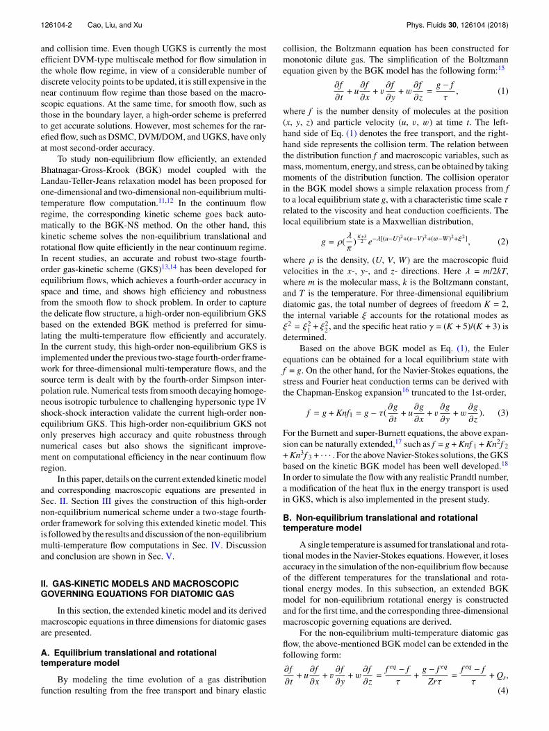
the results from the second order GKS. High order accuracyis achieved in the high order GKS, which has the advan-tage of simulating the non-equilibrium multi-temperature flowwhen the smooth equilibrium region appears. Besides, smalldifference resulting from the different bulk viscosity termbetween the high order equilibrium GKS and high order GKSis observed in this TKE spectral. This different behavior is alsoverified by the PDF of the local Mach number M loc and thecontours of ∆T shown in Fig. 2 as the maximum differencebetween the translational temperature and rotational tempera-ture on the z = 0.5 plane at dimensionless time t∗ = 0.87 is nomore than 1.2%.
B. Low-density nozzle flow
A low-thrust rocket engine has been used for the controlof altitude and trajectory of satellites and spacecrafts. For thistype of rocket engine, the fluid experiences continuum, tran-sition flow regime, which provides a necessary test for thevalidity of the current high order GKS method for the nearcontinuum flow regime.
Low density nozzle flow has been measured using theelectron beam fluorescence technique by Rothe,29 and DSMCsimulations have been performed by Chung et al.30 The flowcondition for the test case is stagnation temperature T0 = 300K, stagnation pressure P0 = 474 Pa, wall temperature Tw =300 K, and the Knudsen number Kn∞ = 5.2 × 10⁻³. This isan axisymmetric flow problem; only one quarter part of thisnozzle has been computed with 340 × 60 × 60 grid pointsused inside the nozzle. An empirical first-order slip boundarycondition31 is used in the current high order GKS method forthe isothermal boundary condition.
Figure 3 shows the Mach contour and non-dimensionaldensity contour inside this nozzle, where the high ratio ofdensity from the inlet to outlet is observed. The experimen-tal data of density and rotational temperature along the nozzlecenterline are shown in Fig. 4. The current high order GKSmethod is validated in the near continuum flow regime as com-putation results provide a close match with the experimentalmeasurement.
FIG. 2. PDF of the local Mach number M loc (left) and contour of ∆T (right) on the z = 0.5 plane at dimensionless time t∗ = 0.87.

126104-9 Cao, Liu, and Xu Phys. Fluids 30, 126104 (2018)
FIG. 3. Mach contour (left) and non-dimensional density contour (right) in the nozzle flow computations.
FIG. 4. Density and rotational temperature distributions along the central line of the nozzle, where Rt is the throat radius. The measured rotational temperatureis from the experiment.29
C. Rarefied hypersonic flow over a flat plate
Physical phenomena occurring around spacecraft in ahypersonic rarefied gas flow are studied in order to understandthese phenomena and to design a real size vehicle. Followingthe experiment conducted by Tsuboi and Matsumoto32 simu-lation on the hypersonic rarefied gas flow over a flat plate isimplemented. The case is run 34, with the nozzle exit Machnumber Ma = 4.89, stagnation temperature T0 = 670 K, stagna-tion pressure P0 = 983 Pa, nozzle exit temperature T e = 116 K,flat plate surface temperature Tw = 290 K with the first-order slip boundary condition used, and the Knudsen numberKn∞ = 6.2 × 10⁻³. The geometry is shown in Fig. 5, where400 × 200 and 300 × 100 grid points above and below the flatplate are used. In this case, the shock wave and boundary layerinteraction near a sharp leading edge causes a non-equilibriumeffect between the translational and rotational temperature inthe rarefied gas regime.
The temperature distributions in the vertical directionabove the flat plate at the locations of x = 5 mm and x = 20 mmfrom the leading edge are shown in Fig. 6. As a comparison,
the UGKS results9 and DSMC results32 are also included. Asshown in Fig. 6, the current high order GKS result is compa-rable with the DSMC result, while the current high order GKSis more efficient than DSMC. However, UGKS results havea perfect match with the experiment measurement than thecurrent high order GKS method and DSMC solution, whichshows its great advantage for multi-scale flow simulation. Herecoarse grids in physical space are used in the UGKS scheme,with 59 × 39 grid points above the plate and 44 × 25 below theplate. However, velocity space is discretized with 80 × 60 gridpoints in the UGKS scheme, so the current high order GKSmethod is still competitive in the near continuum flow regimeconsidering its higher efficiency than UGKS.
D. Type IV shock-shock interaction
Shock-shock interaction is the key issue in hypersonicflow. The presence of intense shock waves’ interaction stronglyaffects vehicle aerodynamic performance and leads to substan-tial localized aerodynamic heating. Shock-shock interaction

126104-10 Cao, Liu, and Xu Phys. Fluids 30, 126104 (2018)
FIG. 5. Translational (left) and rotational (right) temperature contours in the hypersonic flow over a flat plate.
FIG. 6. Rotational temperature distributions in the vertical direction at x = 5 mm (left) and x = 20 mm (right). The measured rotational temperature,32 currenthigh order GKS solutions, UGKS solution,9 and DSMC solution32 are presented.
was classified by Edney33 into six patterns, depending on theimpinging position and angle. In this paper, type IV inter-action is studied, which is the most severe case to form thehot spot on the surface of the cylinder due to the supersonicjet hitting on the wall. The flow patterns of the formation ofa supersonic impinging jet, a series of shock waves, expan-sion waves, and shear layers in a local area of interactionform a pretty challenging case for such a high-order GKSscheme.
An experimental test has been conducted by the OfficeNational d’Etudes et de Recherches Aerospatiales (ONERA)34
to investigate shock-shock interactions, which provides free-stream air flow properties of M∞ = 10, T∞ = 52.5 K,Tw = 300 K, Re∞/m = 1.66 × 10⁵, and the Knudsen numberKn∞ = 5.5 × 10⁻³. The leading edge of the shock generator ispositioned at a distance L = 102 mm upstream of the cylinderand 53 mm below the axis of the cylinder, and the cylinderdiameter is 16 mm. Our simulation is based on 250 × 440grid points around the cylinder. Configuration for the ONERAshock-shock interaction experiment and the Schlieren imagesby density gradient magnitude from the current computation
is shown in Fig. 7. A steady state solution is obtained fromthe high order GKS scheme after a long time iteration with theiterative steps on the order of 105, and the flow structure keepsthe same form.
The translational temperature contour and rotational tem-perature contour around the cylinder are shown in Fig. 8.These contours confirm the existence of multiple temperaturefor this hypersonic flow. More specifically, the Mach num-ber and pressure in the supersonic jet region are shown inFig. 9, which clearly show the strong jet and hot spot aroundthe cylinder surface. Figure 10 presents two horizontal profilesof the measured rotational temperature in the experiment. Oneis located above the upper shock triple point at y = −2 mm,and the other is the line at y = −4 mm, which passes thetransmitted shock and intersects with the surface one degreebelow the location of jet impingement. The high-order GKSresults are close to the DSMC solution35 at y = −2 mm, whileoscillation appears in DSMC simulation. At y = −4 mm, ourcomputational results have a closer match with the experimentthan with the DSMC solution, especially near the x = 0 mmregion.

126104-11 Cao, Liu, and Xu Phys. Fluids 30, 126104 (2018)
FIG. 7. Configuration for the ONERA experiment34 (left) and Schlieren images by density gradient magnitude (right) from the current high order GKS for typeIV shock-shock interaction.
FIG. 8. Translational temperature con-tour (left) and rotational temperaturecontour (right) for type IV shock-shockinteraction.
The non-dimensional pressure and heat flux along thecylindrical surface from experimental measurements,34 thehigh order GKS, and DSMC computational results35 are shown
in Fig. 11, where pc ,s = 760 Pa and qc ,s = 5.7 W/cm2 are thereference values for the undisturbed flow around the cylinder.The experimental heating data set is inadequate to define the
FIG. 9. Local Mach contour (left) and pressure (right) contour in the supersonic jet region.

126104-12 Cao, Liu, and Xu Phys. Fluids 30, 126104 (2018)
FIG. 10. Rotational temperature profile at y = −2 mm (left) and profile at y = −4 mm (right). The measured rotational temperature,34 current high order GKSsolutions, and DSMC solution35 are presented.
FIG. 11. Non-dimensional heating-rate distribution (left) and non-dimensional pressure distribution (right) along the cylindrical surface. The measured rotationaltemperature,34 current high order GKS solutions, and DSMC solution35 are presented.
peak value because of the limited spatial resolution, while thehigh order GKS and DSMC present the close peak positionwith different peak values. In terms of pressure distribution,the high order GKS outweighs DSMC results near 0◦. Nearthe 0◦ region, a slightly low pressure region is found in Fig. 9,which provides confidence on the high accuracy achieved bythe high-order GKS scheme.
The current high-order multi-temperature GKS focuses onhigh-temperature non-equilibrium flow simulation in the near-continuum flow regime efficiently without updating discretevelocity distribution. The GKS method has the similar func-tion as the well-known regularized 13-moment equations36
and the nonlinear coupled constitutive relations (NCCRs)37
for the non-equilibrium flow study with updating macro-scopic flow variables only. As to the extension of the currenthigh-order multi-temperature GKS to rarefied flow, furtherinvestigation and improvements will be considered in futurework.
V. CONCLUSION
In this paper, a high-order three-dimensional multi-temperature GKS method is implemented under the two-stage fourth-order framework. Based on the extended BGKmodel, the three-dimensional macroscopic governing equa-tions for diatomic gas are derived, which provide better insightinto the behavior of the multi-temperature flow. Based onthe developed multiple temperature kinetic model, a corre-sponding high-order GKS is constructed under the two-stagefourth-order framework and the source term discretizationwith the fourth-order Simpson interpolation rule. For non-equilibrium multi-temperature flow computation, decayinghomogeneous isotropic turbulence, nozzle flows, hypersonicrarefied flow over a plate, and type IV shock-shock interactioncases are tested. Comparisons among the numerical solutionsfrom the current high order GKS scheme, UGKS results,DSMC solutions, and experimental measurements show the

126104-13 Cao, Liu, and Xu Phys. Fluids 30, 126104 (2018)
high accuracy and quite robustness of the current numeri-cal method. Most importantly, since the current finite volumegas-kinetic scheme updates the macroscopic flow variablesonly, the GKS can achieve high efficiency in comparison withUGKS and DSMC methods, especially for flow simulation inthe near continuum regime.
ACKNOWLEDGMENTS
We would like to thank Xing Ji for helpful discussionand suggestions about high-order schemes. The authors wouldlike to thank TianHe-II in Guangzhou for providing high per-formance computational resources. The current research issupported by the Hong Kong Research Grant Council (Nos.16207715 and 16206617) and National Science Foundation ofChina (Nos. 11772281 and 91530319).
APPENDIX: CONNECTION BETWEEN BGKAND MACROSCOPIC NON-EQUILIBRIUMMULTI-TEMPERATURE EQUATIONSIN THREE-DIMENSIONS
Derivation of the Navier-Stokes and Euler equations fromthe BGK model can be found in Appendix B.10 For macro-scopic non-equilibrium multi-temperature equations in two-dimensions, it has been derived in previous work.12 Thisappendix provides the details for the derivation of macro-scopic non-equilibrium multi-temperature equations in three-dimensions. In this Appendix, “Eq. (B.x)” represents the pre-liminary equation in Appendix B,10 which will not be rewrittenin the current appendix.
Continuity equation is given by
ρ,t + (ρUk),k = 0, (A1)
which can be used to simplify the momentum equations, thetotal energy equations, and the rotational energy equations.
For momentum equations, the left-hand side L5 inEq. (B2) can be grouped as
L5 =12
U2n [ρ,t + (ρUk),k] + ρUnUn,t + ρUkUnUn,k
+ Ukp,k +K + 3
2[p,t + Ukp,k] +
K + 52
pUk,k
+K2
(pr − p)t +K2
[(pr − p)Uk],k .
The first term is 12 U2
nL1 which is O(ε2), and next three areUnLn and are therefore O(ε). Then L5 can be rewritten as
L5 =K + 3
2[p,t + Ukp,k] +
K + 52
pUk,k + UnLn
+K2{[(pr)t + (prUk),k] − [p,t + (pUk),k]}. (A2)
Based on the Chapman-Enskog expansion up to zero order,the rotational energy equation is obtained as
(ρEr)t + (ρErUk),k =3ρ
2(K + 3)Zrτ(
1λt−
1λr
), (A3)
which can be used to eliminate (pr)t + (prUk),k . Based onpr = ρEr , Eq. (A2) can be rewritten as
−K + 3
2[p,t + Ukp,k] =
K + 52
pUk,k −K2
pUk,k
+K2{[
32(K + 3)Zrτ
(1λt−
1λr
)]
− [p,t + Ukp,k]}
+ UnLn + O(ε).
Finally, we get
p,t +Ukp,k = −53
pUk,k −K ρ
2(K + 3)Zrτ(
1λt−
1λr
)+O(ε), (A4)
which can be used to eliminate p,t + Ukp,k .For the right-hand sides of the momentum equations, we
considerRj = (τFjk),k .
Using the fact that all odd moments in wk vanish, we get
Fjk ≡ 〈ujuk〉,t + 〈ujukul〉,l
= Uj[(ρUk),t + [(ρUkUl) + pδkl],l] + ρUkUj,t + (pδjk),t
+ (ρUkUl + pδkl)Uj,l + (Ulpδjk + Ukpδjl),l.
The term in square brackets multiplying U j isLk , i.e., it isO(ε),and can therefore be ignored. Then, after gathering terms withcoefficients Uk and p, we have
Fjk = Uk[ρUj,t + ρUlUj,l + p,j] + p[Uk,j + Uj,k + Ul,lδjk]
+ δjk[p,t + Ulp,l].
The coefficient of Uk isLj, according to Eq. (B7), and cantherefore be neglected. To eliminate p,t from the last term, weuse Eq. (A4) for L5. Finally, decompose the tensor Uk ,j intoits dilation and shear parts in the usual way, which gives
Fjk = [Uk,j +Uj,k−23
Ul,lδjk]−K ρ
2(K + 3)Zr(
1λt−
1λr
)δjk . (A5)
Analogy to deriving the Navier-Stokes total energy equa-tion, we write
Nk ≡ 〈uku3
n + ξ2r
2〉,t + 〈ukul
u3n + ξ2
r
2〉,l,
which can be written as
Nk = N (1)k + N (2)
k ,
where
N (1)k = [Uk
u3n + ξ2
r
2],t + [Uk〈ul
u3n + ξ2
r
2〉],l,
and
N (2)k ≡ 〈wk
u3n + ξ2
r
2〉,t + 〈wkul
u3n + ξ2
r
2〉,l .
For N (1)k , we have
N (1)k = Uk[
12〈u2
n + ξ2r 〉,t +
12〈ul(u
2n + ξ2
r )〉,l]
+ [12ρU2
n +K + 3
2p]Uk,t + [Ul(
12ρU2
n +K + 5
2p)]Uk,l
+K2
(pr − p)Uk,t +K2
Ul(pr − p)Uk,l.

126104-14 Cao, Liu, and Xu Phys. Fluids 30, 126104 (2018)
The coefficient of Uk in the equation above isL5 and there-fore can be dropped, and the remaining terms can be rewrittenas
N (1)k = [
12ρU2
n +K + 3
2p][Uk,t + UlUk,l] + pUlUk,l.
According to Eq. (B7) to eliminate Uk ,t , we get
N (1)k = −[
12
U2n +
K + 32
pρ
]p,k + pUlUk,l
+K2
(pr − p)Uk,t +K2
Ul(pr − p)Uk,l. (A6)
For N (2)k , remembering that moments odd in wk vanish,
we have
N (2)k = 〈Unwnwk〉,t + 〈UlUnwnwk〉,l
+12〈U2
nwkwl〉,l +12〈wkwl(w
2n + ξ2
r )〉,l
= (pUk),t + (pUkUl),l +12
(U2n p),k
+K + 5
2(p2
ρ),k +
K2
(p(pr − p)
ρ),k .
This result can be written as
N (2)k = p[Uk,t + UlUk,l + UkUl,l + UlUl,k]
+ Uk(p,t + Ulp,l) +12
U2n p,k +
K + 52
(p2
ρ),k
+K2
(p(pr − p)
ρ),k .
To eliminate the first order time derivative, we can rearrangethe above equality as
N (2)k = p[Uk,t + UlUk,l + UkUl,l + UlUl,k]
+ Uk(p,t + Ulp,l) +12
U2n p,k +
K + 52
(p2
ρ),k
+K2
(p(pr − p)
ρ),k .
Uk ,t can be eliminated by Eq. (B7), and p,t + U lp,l can beeliminated by Eq. (A4).
Hence
N (2)k = p[UkUl,l −
p,k
ρ+ UlUl,k]
+ Uk[−53
pUl,l −K
(K + 3)Zrτ(p − pr)]
+12
U2n p,k +
K + 52
(p2
ρ),k +
K2
(p(pr − p)
ρ),k . (A7)
For Nk , sum up N (1)k and N (2)
k together, obtaining
Nk = p[Ul(Uk,l + Ul,k) −23
UkUl,l] − UkK
(K + 3)Zrτ(p − pr)
+K + 5
2p(
pρ
),k +K2
(pr − p)Uk,t
+K2
Ul(pr − p)Uk,l +K2
(p(pr − p)
ρ),k .
Eliminate Uk ,t by Eq. (B7) again, leading to
Nk = p[Ul(Uk,l + Ul,k) −23
UkUl,l] − UkK
(K + 3)Zrτ(p − pr)
+K2
p(pr
ρ),k +
52
p(pρ
),k . (A8)
For rotational energy equation, multiplying the continuityequation [Eq. (A1)] by K
4λrand the subtracting the result from
Eq. (A3) give
L6 = ρ(K
4λr)t + ρUk(
K4λr
)k −3ρK
4(K + 3)Zrτ(
1λt−
1λr
) +O(ε2).
(A9)Unfolding R6 leads to
R6 =∂
∂xk{τ[〈
12ξ2
r uk〉,t + 〈12ξ2
r ukul〉,l]}
= τ{ K4λr
[(ρUk),t + (ρUkUl + pδk,l),l]
+ ρUk(K
4λr)t + (
K4λr
),l[ρUkUl + pδkl]}
,k .
The term in square brackets is Lk , i.e., O(ε), and can bedropped. Gathering terms with coefficients Uk and p, andeliminating ρ( K
4λr)t + ρUl( K
4λr),l by Eq. (A9), we have
R6 = τ{Uk[ρ(K
4λr)t + ρUl(
K4λr
),l] + (K
4λr),lpδkl},k
= τ{Uk[3ρK
4(K + 3)Zr(
1λt−
1λr
)] + (K
4λr),lpδkl},k . (A10)
Above equations can be rewritten in the form of Eq. (10).Hence, macroscopic non-equilibrium multi-temperature equa-tions to three-dimensions have been derived.
1M. Ivanov and S. Gimelshein, “Computational hypersonic rarefied flows,”Annu. Rev. Fluid Mech. 30, 469–505 (1998).
2G. Bird, Molecular Gas Dynamics and the Direct Simulation Monte Carloof Gas Flows (Clarendon, Oxford, 1994), Vol. 508, p. 128.
3J. Yang and J. Huang, “Rarefied flow computations using nonlinear modelBoltzmann equations,” J. Comput. Phys. 120, 323–339 (1995).
4L. Mieussens, “Discrete-velocity models and numerical schemes forthe Boltzmann-BGK equation in plane and axisymmetric geometries,”J. Comput. Phys. 162, 429–466 (2000).
5Z.-H. Li and H.-X. Zhang, “Gas-kinetic numerical studies of three-dimensional complex flows on spacecraft re-entry,” J. Comput. Phys. 228,1116–1138 (2009).
6L. Yang, C. Shu, W. Yang, Z. Chen, and H. Dong, “An improved discretevelocity method (DVM) for efficient simulation of flows in all flow regimes,”Phys. Fluids 30, 062005 (2018).
7K. Xu and J.-C. Huang, “A unified gas-kinetic scheme for continuum andrarefied flows,” J. Comput. Phys. 229, 7747–7764 (2010).
8J.-C. Huang, K. Xu, and P. Yu, “A unified gas-kinetic scheme for continuumand rarefied flows. III: Microflow simulations,” Commun. Comput. Phys.14, 1147–1173 (2013).
9S. Liu, P. Yu, K. Xu, and C. Zhong, “Unified gas-kinetic scheme for diatomicmolecular simulations in all flow regimes,” J. Comput. Phys. 259, 96–113(2014).
10K. Xu, Direct Modeling for Computational Fluid Dynamics: Constructionand Application of Unified Gas-kinetic Schemes (World Scientific, 2015).
11K. Xu and E. Josyula, “Continuum formulation for non-equilibrium shockstructure calculation,” Commun. Comput. Phys. 1, 425–450 (2006).
12K. Xu, X. He, and C. Cai, “Multiple temperature kinetic model andgas-kinetic method for hypersonic non-equilibrium flow computations,”J. Comput. Phys. 227, 6779–6794 (2008).
13J. Li and Z. Du, “A two-stage fourth order time-accurate discretization forLax–Wendroff type flow solvers. I. Hyperbolic conservation laws,” SIAMJ. Sci. Comput. 38, A3046–A3069 (2016).

126104-15 Cao, Liu, and Xu Phys. Fluids 30, 126104 (2018)
14L. Pan, K. Xu, Q. Li, and J. Li, “An efficient and accurate two-stagefourth-order gas-kinetic scheme for the Euler and Navier–Stokes equations,”J. Comput. Phys. 326, 197–221 (2016).
15P. L. Bhatnagar, E. P. Gross, and M. Krook, “A model for collision processesin gases. I. Small amplitude processes in charged and neutral one-componentsystems,” Phys. Rev. 94, 511 (1954).
16S. Chapman, T. G. Cowling, and D. Burnett, The Mathematical Theory ofNon-uniform Gases: An Account of the Kinetic Theory of Viscosity, ThermalConduction and Diffusion in Gases (Cambridge University Press, 1990).
17T. Ohwada and K. Xu, “The kinetic scheme for the full-Burnett equations,”J. Comput. Phys. 201, 315–332 (2004).
18K. Xu, “A gas-kinetic BGK scheme for the Navier–Stokes equations andits connection with artificial dissipation and Godunov method,” J. Comput.Phys. 171, 289–335 (2001).
19J. Parker, “Rotational and vibrational relaxation in diatomic gases,” Phys.Fluids 2, 449–462 (1959).
20K. Koura, “Statistical inelastic cross-section model for the Monte Carlosimulation of molecules with discrete internal energy,” Phys. Fluids A 4,1782–1788 (1992).
21G.-S. Jiang and C.-W. Shu, “Efficient implementation of weighted ENOschemes,” J. Comput. Phys. 126, 202–228 (1996).
22Q. Li, K. Xu, and S. Fu, “A high-order gas-kinetic Navier–Stokes flowsolver,” J. Comput. Phys. 229, 6715–6731 (2010).
23G. Comte-Bellot and S. Corrsin, “Simple Eulerian time correlation of full-and narrow-band velocity signals in grid-generated, ‘isotropic’ turbulence,”J. Fluid Mech. 48, 273–337 (1971).
24A. Vreman, “An eddy-viscosity subgrid-scale model for turbulent shearflow: Algebraic theory and applications,” Phys. Fluids 16, 3670–3681(2004).
25U. Baro, S. Mahapatra, S. Ghosh, and R. Friedrich, “Les of supersonicminimal channel flow between isothermal walls at different temperaturesincluding thermal radiation effects using a fictitious gray gas,” Phys. Fluids30, 015103 (2018).
26M. Righi, “A gas-kinetic scheme for turbulent flow,” Flow, Turbul. Combust.97, 121–139 (2016).
27S. Tan, Q. Li, Z. Xiao, and S. Fu, “Gas kinetic scheme for turbulencesimulation,” Aerosp. Sci. Technol. 78, 214–227 (2018).
28G. Cao, H. Su, J. Xu, and K. Xu, “Implicit high-order gas kinetic schemefor turbulence simulation,” e-print arXiv:1811.08005.
29D. E. Rothe, “Electron-beam studies of viscous flow in supersonic nozzles,”AIAA J. 9, 804–811 (1971).
30C.-H. Chung, S. C. Kim, R. M. Stubbs, and K. J. De Witt, “Low-densitynozzle flow by the direct simulation Monte Carlo and continuum methods,”J. Propul. Power 11, 64–70 (1995).
31J. C. Maxwell, “VII. On stresses in rarified gases arising from inequalitiesof temperature,” Philos. Trans. R. Soc. London 170, 231–256 (1879).
32N. Tsuboi and Y. Matsumoto, “Experimental and numerical study ofhypersonic rarefied gas flow over flat plates,” AIAA J. 43, 1243–1255(2005).
33B. Edney, “Anomalous heat transfer and pressure distributions on bluntbodies at hypersonic speeds in the presence of an impinging shock,”Technical Report No. FFA-115, Flygtekniska Forsoksanstalten, Stockholm,Sweden, 1968.
34T. Pot, B. Chanetz, M. Lefebvre, and P. Bouchardy, “Fundamental study ofshock/shock interference in low density flow- flow field measurements byDLCARS,” in 21st International Symposium on Rarefied Gas Dynamics,Marseille, France 26–31 July 1998 (ONERA, TP, 1998), 1998-140.
35J. Moss, T. Pot, B. Chanetz, and M. Lefebvre, “DSMC simulationof shock/shock interactions: Emphasis on type IV interactions,” NASALangley Technical Report No. 20040086965 (1999).
36M. Torrilhon and H. Struchtrup, “Regularized 13-moment equations: Shockstructure calculations and comparison to Burnett models,” J. Fluid Mech.513, 171–198 (2004).
37N. Le, H. Xiao, and R. Myong, “A triangular discontinuous Galerkin methodfor non-Newtonian implicit constitutive models of rarefied and microscalegases,” J. Comput. Phys. 273, 160–184 (2014).