HAL Id: hal-00746982https://hal.archives-ouvertes.fr/hal-00746982

Submitted on 30 Oct 2012

HAL is a multi-disciplinary open accessarchive for the deposit and dissemination of sci-entific research documents, whether they are pub-lished or not. The documents may come fromteaching and research institutions in France orabroad, or from public or private research centers.

L’archive ouverte pluridisciplinaire HAL, estdestinée au dépôt et à la diffusion de documentsscientifiques de niveau recherche, publiés ou non,émanant des établissements d’enseignement et derecherche français ou étrangers, des laboratoirespublics ou privés.

Physical properties and giant magnetoimpedancesensitivity of rapidly solidified magnetic microwires

Basile Dufay, Sébastien Saez, Christophe Dolabdjian, Arthur Yelon, DavidMénard

To cite this version:Basile Dufay, Sébastien Saez, Christophe Dolabdjian, Arthur Yelon, David Ménard. Physical proper-ties and giant magnetoimpedance sensitivity of rapidly solidified magnetic microwires. Journal of Mag-netism and Magnetic Materials, Elsevier, 2012, 324 (13), pp.2091-2099. 10.1016/j.jmmm.2012.02.012.hal-00746982

Physical properties and giant magnetoimpedance sensitivity of rapidly

solidied magnetic microwires

B. Dufaya,b,c,d,∗, S. Saeza,b,c, C. Dolabdjiana,b,c, A. Yelond, D. Ménardd

aUniversité de Caen Basse-Normandie, UMR 6072 GREYC, F-14032 Caen, FrancebENSICAEN, UMR 6072 GREYC, F-14050 Caen, France

cCNRS, UMR 6072 GREYC, F-14032 Caen, FrancedÉcole Polytechnique de Montréal, département de génie physique & regroupement québécois des matériaux de pointe,

Montréal, Québec, Canada H3C3A7

Abstract

The relation between the magnetoimpedance and the magnetic properties of a wide set of soft magneticmicrowires from several sources has been studied. Magnetic properties were obtained by vibrating samplemagnetometry and ferromagnetic resonance spectroscopy. The magnetoimpedance voltage sensitivity ofeach sample, the criterion of interest for high sensitivity magnetometer design, was then evaluated at severalfrequencies and drive currents. It appears that all samples possess roughly similar properties, regardlessof their fabrication process or chemical composition. The voltage sensitivity of the samples obtained fromexperimental measurement is compared with a simple model of sensitivity. The general trends predictedby the model provide useful insights for materials optimization. Averaged sensitivity over the sample setis around 10 kV/T/cm at 10 MHz. The critical importance for sensitive magnetometry of the maximumexcitation current permissible in each wire is also highlighted.

Keywords: Giant Magnetoimpedance (GMI), Voltage Sensitivity, Magnetometry, Soft Amorphous Wires,Ferromagnetic resonance, Magnetic Sensors.

1. Introduction

The giant magnetoimpedance (GMI) eect hasattracted great attention in the past two decades,due to its potential for the design of low cost, highperformance, magnetometers [1]. Much of the eorttoward optimization of GMI materials has been di-rected towards increasing the amplitude of the rel-ative impedance variation with respect to the ex-ternal applied magnetic eld,

∆Z

Zref=

Z − Zref

Zref(1)

in relation to a reference value, Zref . The latter isgenerally chosen to be the impedance at zero eld,or at the maximum available eld. As was recentlydiscussed [2], this GMI ratio, Eq. (1), is not partic-ularly meaningful as a metric for sensitive magne-tometry and it can be misleading in the comparison

∗Corresponding authorEmail address: basile.dufay@unicaen.fr (B. Dufay)

of the performance between GMI wires from dier-ent sources.

Here, we adopt the pragmatic point of view thatthe main criterion relevant to the design of highlysensitive GMI magnetometers is the maximum volt-age sensitivity, dened as the dierential variationof voltage across the GMI sample, divided by theapplied magnetic eld, expressed in V/T [2, 3].This value is related to the dierential variationin impedance, which we may also call the intrinsicimpedance sensitivity, SΩ/T

max

= ∂Z/∂B|B=Bopt,

evaluated under optimal bias eld, Bopt (= µ0Hopt),and optimal AC drive current, IAC−opt, permissi-ble in the wire. We emphasize that, in order tobe meaningful, the response must be measured un-der optimal bias and driving conditions. In highsensitivity magnetometer design, a high signal-to-noise ratio (SNR) is extremely important. Thus, avoltage sensitivity as high as possible is clearly de-sirable whenever the dominant noise source is thatof the electronic conditioning circuitry, as has been

Preprint submitted to Elsevier December 13, 2011

Figure 1: Modulus of the impedance variation versus appliedmagnetic eld, from [2]. The black solid straight line repre-sents the maximum slope, that is the intrinsic impedancesensitivity. The dotted line is the approximation for slopeused in the simple model of sensitivity.

observed [3, 4].Ménard and collaborators [2] have proposed a

model in order to establish simple relations betweenGMI sensitivity and material parameters, alongwith driving current and frequency. The maximumvoltage sensitivity, in units of V/T, is reached atthe optimal driving current and external bias eld.It is estimated from

SV/Tmax

= SV/T(IAC−opt, Bopt) (2)

= IAC−optSΩ/Tmax

≈ IAC−optZpk

µ0Hpk.

That is, it was approximated as the ratio of maxi-mum impedance value, Zpk, over its eld position,Hpk, as illustrated in Fig. 1. In the strong skin ef-fect regime, for a monodomain soft magnetic wire,of length l, and with a perfectly circumferentialanisotropy within the skin depth region, the volt-age sensitivity, per unit length, may be estimatedusing [2]

SV/Tmax

l≈

(

M2sωρ

3

µ20A

)1/4 [Hcrit(ω)

Hpk(ω)

]

(ω ≤ ωc)

(3a)

SV/Tmax

l≈

(

γMsρ

α

)1/2 [Hcrit(ω)

Hpk(ω)

]

(ω ≥ ωc)

(3b)

where ω is the excitation angular frequency, Ms isthe saturation magnetization of the sample, ρ isits resistivity, α is the Gilbert damping parame-ter, γ is the gyromagnetic ratio, A is the exchangestiness constant (approximately 10−11 J/m) and

Hcrit is the critical surface magnetic eld related tothe optimal driving current, IAC−opt = 2πaHcrit.The angular frequency, ωc, is the crossover fre-quency, above which the maximum impedanceis no longer limited by exchange-conductivity ef-fects (equation (3a)), but by phenomenologicalGilbert damping (equation (3b)). The eld ratio,Hcrit/Hpk, is on the order of unity for ideal wires inthe quasi-static regime. At higher frequency, bothelds increase with increasing frequency, but Hcrit

increases faster than Hpk. In what follows, we as-sume conservatively that this eld ratio is roughlyunity in the frequency range considered.While Eqs. (3a) and (3b) are likely to be too sim-

ple to comprehend all the subtleties of the GMI ef-fect, they provide useful design rules for materialand sensor optimization. Indeed, the voltage sensi-tivity per unit length, measured under optimal driv-ing condition, is a material-dependent and radius-independant metric to gauge the merit of dierentsamples. It is also important to note that for real(non-ideal) wires, which do not exhibit perfect cir-cumferential anisotropy, the maximum impedancevariation is more likely to be described by an eec-tive Gilbert damping parameter, corresponding toa sensitivity given by (3b) at all frequencies.Here, we confront this simple model by analyzing

and comparing a set of dierent GMI microwires,fabricated in dierent laboratories. The emphasis isplaced on the relation between voltage sensitivitiesand physical properties. This required us to mea-sure the physical properties of the wires. Therefore,a signicant part of the discussion is dedicated tothe proper determination of the relevant physicalproperties (material parameters) of rapidly solidi-ed microwires. Section 2 describes the experimen-tal details and data analysis. The measured phys-ical properties are presented in Sec. 3. Sensitivityperformances are discussed and compared in Sec. 4,which is followed by a general conclusion.

2. Experimental

2.1. Materials and sample preparation

A set of ten dierent samples of soft amorphousmicrowires with dierent chemical compositions(essentially based on CoFeSiB alloys except for sam-ple a2) and made by three dierent fabrication pro-cesses were selected for this study. The samplesare described in Table 1. The rst three samples,a1 to a3, were obtained by melt-extraction [5] and

2

were provided by MXT, in Montréal. Samples b1to b4 are glass-covered amorphous wires [6] with athin glass coating, provided by the department ofFisica de Materiales UPV/EHU (San Sebastian).Samples c1 to c3, from the Institute of R&D forTechnical Physics (Iasi, Romania), consist of twoglass-covered wires with thick glass coating and onewith large radius, obtained by quenching in rotat-ing water [7]. The exact composition of the alloysfrom the third provider is unknown. Let us em-phasize that the samples were chosen to provide avariety of fabrication methods and physical prop-erties, but were not necessarily optimized for GMIapplications. A permalloy and a metglas microwire,from MXT, part of the original set, are not includeddue to their poor GMI behavior.

In order to compare the measured GMI sensitiv-ity to the results of the model outlined in the intro-duction, we have measured the following relevantphysical properties: the saturation magnetization,Ms, the resistivity, ρ, the Gilbert damping param-eter, α, and the Landé-factor, g = γ~/µB where γis the gyromagnetic ratio, µB the Bohr magnetonand ~ the reduced Planck constant. In addition,we measured the coercive magnetic eld, HC , as anindicator of the soft magnetic behavior. The sam-ples were also characterized regarding their intrin-sic impedance sensitivity, SΩ/T(µ0H), and voltagesensitivity, SV/T(IAC , µ0H).

First, a 7 cm segment of each material was cut fordetermination of its DC resistance per unit length,using a 4-point measurement setup. Radius, a, wasestimated using optical microscopy. For samplesb1 to c3, a nominal radius was also provided bythe supplier. Values of the resistances, lengths anddiameters yielded the electrical resistivity.

Each 7 cm segment was subsequently cut intothree parts. The rst, about 0.5 cm long, was usedfor vibrating sample magnetometry (VSM), the sec-ond, less than 0.2 cm long, was dedicated to ferro-magnetic resonance measurement (FMR). The re-maining segment was cut into 1.5 cm long samples,which were soldered onto a sample holder for de-termination of GMI response. As the estimation ofradii by optical microscopy was found to be impre-cise, we used the magnetic characterization to de-rive the diameter, as explained below. The follow-ing subsections explain the various characterizationprocedures.

2.2. Vibrating Sample Magnetometry (VSM)

The static magnetic properties were investigatedusing a vibrating sample magnetometer (VSM). Weobtained the magnetic moment as a function of ex-ternal applied eld for each sample for various an-gles, θH , between the applied eld and the wire axis.In Fig. 2, we show a representative curve of thenormalized magnetization as a function of eld forparallel, θH = 0, and perpendicular, θH = π

2, elds

(sample a1). For each sample, we measured thelongitudinal coercive eld, HC , and the normalizedapparent susceptibility (slope ∂(M/Ms)/∂H|M=0

),χ‖ and χ⊥, for both magnetization directions as il-lustrated in Fig 2. Only the parallel and perpen-dicular eld results were retained for this work.The VSM was calibrated using a Ni disk as ref-

erence. The saturation magnetization, Ms, may beestimated from the maximum value of the measuredmagnetic moment, |−→m|, from

Ms =|−→m|

lπa2(4)

where lπa2 represents the volume of the sample un-der measurement. While this is the most directevaluation of the saturation magnetization, uncer-tainties as to the length and, mainly, the diameterplace limits on its usefulness.Another estimate can be obtained by extrapolat-

ing the linear portion of the magnetization curveto saturation, and assuming that the eld at satu-ration is equal to the demagnetization eld, Ms/2.An alternative version of this approach was recentlyproposed [8] for samples for which the magnetiza-tion processes are dominated by the dipolar elds.It is assumed that such samples should exhibit ap-parent initial susceptibilities, χi, given by

Mi = χiH = χ0(H −NiMi), (5)

where χ0 is an isotropic intrinsic susceptibility,i =‖ or ⊥ and Ni is the demagnetization factor.Assuming that N‖χ‖ ≪ 1, which implies that N⊥

is approximately 1/2, then

χ‖ ≈ χ0, (6a)

χ⊥ ≈ χ0

(

1−1

2χ⊥

)

. (6b)

Dening a normalized susceptibility, χi = χi/Ms,and combining Eqs. (6a) and (6b),

χ⊥ = χ‖

(

1−1

2χ⊥Ms

)

. (7)

3

Table 1: Sample description.

Sample Compositioni Fabrication Diameter 2a Other

a1 Co70.54Fe3.95Si15.91B7.13Nb2.91 melt extracted 35 µmii

a2 Ni45Co25Fe6Si9B13Mn2 melt extracted 17 µmii Ni richa3 Co71Fe4Si13.5B6.5Nb5 melt extracted 35 µmii

b1 Co67Fe3.9B11.5Si14.5Ni1.5Mo1.6 thin glass-covered 21.4 µmiii 2.4 µm glassb2 Co67Fe3.9B11.5Si14.5Ni1.5Mo1.6 thin glass-covered 16.4 µmiii 1.5 µm glassb3 Co67Fe3.9B11.5Si14.5Ni1.5Mo1.6 thin glass-covered 25.6 µmiii 0.5 µm glassb4 Co66Fe4B14Si15Ni1 thin glass-covered 22.6 µmiii 2.0 µm glassc1 CoFeSiB thick glass-covered 20 µmiii 13.5 µm glassc2 CoFeSiB thick glass-covered 27 µmiii 21.5 µm glassc3 CoFeSiB rotating water 100 µmiii Large radius

iExact compositions of samples c1 to c3 are unknown.iiEstimated value from optical microscopy.

iiiNominal value provided by the supplier.

Figure 2: Normalized magnetization loops of the sample a1 for two applied eld angle, θH = 0 and θH = π2. It illustrates

deduced characteristics, HC , and χ‖. Note that the eld scale of the two images diers by approximately 1000.

4

Solving Eq. (7) for Ms, we nd

Ms = 21− χ⊥/χ‖

χ⊥, (8)

which provides an experimental value for the mag-netization, independent of our knowledge of thesample volume. For ultra-soft wires with smalldiameter-to-length ratio, the above analysis simpli-es to assuming an apparent perpendicular suscep-tibility of 2 (1/N⊥ with N⊥ = 1/2), so that the sat-uration magnetization is approximately 2χ⊥. As acorollary, combining Eqs. (8) and (4) yields an es-timation of the magnetic volume. Since the lengthand the magnetization of the samples are measuredwith a relatively fair accuracy, the procedure thusleads to experimental values of the wire radii, whichare far more reliable than the values obtained fromoptical microscopy.VSM measurements were also used to investigate

the approach to saturation for each sample. Thiscan be related to imperfections of the materials andmay serve as a discriminant between samples. Forideal samples with uniaxial anisotropy, approachingsaturation by coherent rotation, we would expect alaw of the form M(H) = Ms

(

1− b/H2)

[9], whereb is related to the anisotropy constant and directionof the applied eld relative to the anisotropy axis.However, in real (non-ideal) materials, it is com-mon to observe behavior following forms such asM(H) = Ms

(

1− c/Hβ − ...)

where the exponentβ is related to various defects of the materials [1012]. The parameter β thus provides an indicationof non-ideality of the samples. By rewriting theM(H) formula as log(1−M/Ms) = log c−β logH,one may obtain the power law from the slope of thelogarithmic plot of (1−M/Ms) versus 1/H as illus-trated in Fig. 3. All of the observed values (Table 2)range between 1/2 and 1.

2.3. Ferromagnetic Resonance measurement(FMR)

The microwave response of each sample was in-vestigated in order to observe the ferromagneticresonance (FMR) and ferromagnetic antiresonance(FMAR). Spectra were obtained at room tempera-ture for dierent eld angles using the same equip-ment and procedure described in [8], using a cylin-drical resonant cavity at 38 GHz. We focus hereon axially (θH = 0) magnetized wires. Microwireswere placed in a region with nearly zero dynamicelectric eld and maximum dynamic magnetic eld,

Figure 3: Evaluation of the exponent of the law-of-approach-to-saturation from magnetization curve of the sample a1,obtained by VSM measurement.

linearly polarized transverse to the wire axis. Fromthe spectra of axially magnetized wires, we deducedthe FMR eld, Hr, FMAR eld, Har, and resonantlinewidth, ∆H. Figure 4 illustrates the extractionof these parameters for sample a1. For microwires,it has been shown [13] that the skin eect com-bined with dipolar interactions yields a FMR eldposition given by the Kittel equation [14, 15] forin-plane static eld and insulating thin lms, andthe FMAR is given, for the same conditions, byVan Vleck [15]

(

ω

γµ0

)2

= Hr (Hr +Ms) , (9a)

ω

γµ0

= Har +Ms. (9b)

From the FMR and FMAR elds at a given fre-quency, one can deduce the saturation magnetiza-tion, Ms, and the gyromagnetic ratio, γ. In con-trast, the FMR linewidth, which is a measure ofmagnetic losses, strongly depends upon microwireproperties. It is linked to the Gilbert damping pa-rameter, α, and to eddy current losses. A compre-hensive analysis of the FMR response of microwiresin this experimental conguration was recently pro-posed [16]. Here, the Gilbert damping parame-ters were deduced by tting the FMR experimentalcurves based on the analysis of ref. [16].

2.4. Magnetoimpedance

Magnetoimpedance, Z(H), in the linear regimewas measured using a network analyzer as described

5

Figure 4: Ferromagnetic resonance absorption spectrum ofthe sample a1. The extraction of Hr, Har, and ∆H fromthis measurement are illustrated.

in [17]. Measurements were obtained for several DCbias currents, IDC , (from −10 to 10mA) and sev-eral excitation frequencies, f (3 MHz to 300 MHz).Intrinsic impedance sensitivity, expressed as Ohmsper Tesla, SΩ/T(µ0H), in the magnetic eld range,was then evaluated by numerical dierentiation, asshown in Fig. 5. The use of a DC bias currentresults in an eective eld with helical symmetry,which produces the observed asymmetric response.Measurements in the linear regime enabled us todetermine the optimal DC bias current, which max-imizes the intrinsic impedance sensitivity, for eachsample. This current was then used in the measure-ment of the voltage sensitivity as described below.

The simplied model of the sensitivity presentedin Eqs. (3a) and (3b) assumes that the sample isoperated under an optimal excitation current am-plitude, above which the sensitivity begins to de-crease. Both experiment and calculation [18] showthat the value of this optimal excitation current isslightly larger than the value for the onset of non-linear behavior, and tends to increase with increas-ing operating frequency.

Consequently, the voltage sensitivity was evalu-ated under various sine excitation current ampli-tudes, IAC , by numerical dierentiation of the mea-sured voltage, V (H), at the sample terminals, ver-sus applied magnetic eld. The setup used is de-scribed in [18]. Wires were subjected to the optimalDC bias current deduced from intrinsic impedancesensitivity characterization. Excitation current fre-quency, f , was varied from 300 kHz to 10 MHz.

3. Results: physical properties

The measured physical properties of each sampleare summarized in Table 2. All samples exhibit typ-ical values for soft magnetic metals. The diameterswere determined from the magnetic volume, as dis-cussed in Section 2.2. While some discrepancies areobserved as compared to nominal or optically mea-sured values, one must keep in mind that uctua-tions of diameters are common in soft amorphousmicrowires. The presence of such uctuations isalso suggested by our electrical resistance measure-ments of dierent pieces of microwires of the samecomposition, which exhibits signicant variations.The resistances reported in Table 2 refer to 7 cmlong samples and are not necessarily always repre-sentative of the resistance of the smaller wires cutfrom it and used in the GMI experiments. With thisin mind, values reported for the resistivity, calcu-lated from the estimated resistance and diameters,are, therefore, not always very precise. If we con-sider the uctuations of the DC resistance and thegeometrical parameters, the level of condence inthe resistivity evaluation is not better than 20%.Saturation magnetization was obtained both

from VSM data (Eq. (8)) and FMR data (Eqs. (9a)and (9b)). As anti-resonance was not observed inthe FMR spectra for sample b1 to b4, the Landéfactor could not be determined. The saturationmagnetization for these samples was thus deter-mined using Eq. (9a) with an assumed Landé factorof 2.12, corresponding to the average value of theother samples with similar composition. Gilbert pa-rameters, α, are all between 0.01 and 0.02, which isalso on the order expected for such materials.Evaluation of the saturation magnetization from

Eqs. (8) (VSM) and (9a)-(9b) (FMR) are in a fairlygood agreement. This is illustrated in Fig. 6 whichcompares the dierent values obtained for eachsample. In contrast, Ms determined using Eq. (4),from the saturated magnetic moment measured inthe VSM and the diameters reported in Table 1,tends to be considerably lower. This is another in-dication that the nominal or optically measured di-ameters might be misleading. In what follows, weuse the value of Ms obtained from Eq. (8) (VSM),close to that of Eqs. (9a) and (9b) (FMR).As expected for soft magnetic materials, the sus-

ceptibilities are high and the coercive elds are low(smaller than 4A/m) except for samples a1 and a2for which HC is greater than 15A/m. We note thatboth the susceptibility and coercive elds are struc-

6

Figure 5: Impedance variation, Z(H), versus applied magnetic eld for sample a1, measured using a vector network analyzerat an excitation frequency of 3 MHz and several DC bias currents, IDC . Maximum intrinsic impedance sensitivity, SΩ/T

max

,is determined by numerical dierentiation.

Table 2: Measured physical properties of each sample.

2ai RDC/l Ms (VSM)ii Ms (FMR)iii χ‖ α g ρ HC β

Sample µm Ω/cm kA/m kA/m µΩ.cm A/m

a1 35.8 12.7 558 549 2520 0.011 2.10 128 15.9 2/3

a2 15.3 40 446 445 11640 0.010 2.12 74 15.9 2/3

a3 30.0 19.4 548 561 2700 0.012 2.12 137 3.6 2/3

b1 19.3 40 507 475iv 2910 0.015 2.12v 118 3.6 1/2

b2 12.7 65.7 473 454iv 2480 0.014 2.12v 83 2.0 1/2

b3 24.2 37.1 442 475iv 4030 0.012 2.12v 171 3.2 1/2

b4 20.8 38.6 489 496iv 1600 0.013 2.12v 131 2.8 1/2

c1 17.8 42.9 552 598 4160 0.011 2.11 107 3.6 2/3

c2 26.4 23.7 566 560 2540 0.012 2.15 130 2.4 1/2

c3 102 1.6 542 561 200 0.020 2.11 129 2.4 1

iMagnetic diameter.iiEstimated from equation (8).iiiEstimated from equations (9a) and (9b).ivConsidering an assumed value of g = 2.12.vAssumed value.

7

Figure 6: Measured saturation magnetization values for eachsample from three methods.

ture sensitive properties, which may be aected notonly by the composition and fabrication method,but also by the residual strains or the presence ofdefects which may be introduced during fabricationor during mounting for measurement. Likewise, theanisotropy is aected by the strains of fabricationand mounting. In the case of glass-covered wires,the glass and metal exert strains on each other.

Finally, three dierent power law exponents forapproach to saturation of the magnetization havebeen obtained, as shown in the last column of ta-ble 2 . Departures from an ideal 1/H2 (β = 2) [9]law for uniaxial amorphous materials may be inter-preted as due to inhomogeneities in composition,or induced by magnetoelastic interactions with in-homogeneous stresses [12], or to surface rough-ness [19]. This exponent appears to be somewhatcorrelated to source and preparation method.

Except for sample a2, which has a compositionsignicantly dierent from the others, most CoFe-based samples exhibit similar properties, yet thereare variations, which cannot be accounted for bymeasurement uncertainties. For instance, an av-erage resistivity around 130 µΩ.cm is generally ob-served. Exceptions are sample b2 which shows anunusually low value, of 83 µΩ.cm, and samples c1(107 µΩ.cm) and b3 (171 µΩ.cm) which are some-what lower and higher than average. The sat-uration magnetization also exhibits small varia-tions from sample to sample. The b-series (nomi-nally with identical compositions) have average Ms

of 480 kA/m, signicantly smaller than the valuesof the other CoFe-rich samples which are around

560 kA/m. The average phenomenological Gilbertdamping parameter is approximately 0.012 (exceptfor the larger wire α = 0.020) and Landé factors areall slightly higher than 2, regardless of the fabrica-tion process and chemical composition. As pointedout in the introduction, the sensitivity of non idealwires in the MHz regime is likely to be described byan eective Gilbert damping parameter in Eq. (3b),which could be signicantly higher than that whichis measured in the GHz regime. Nevertheless, α re-mains a meaningful indicator of the microstructuralquality of the samples.

4. Measured and theoretical voltage sensi-

tivity

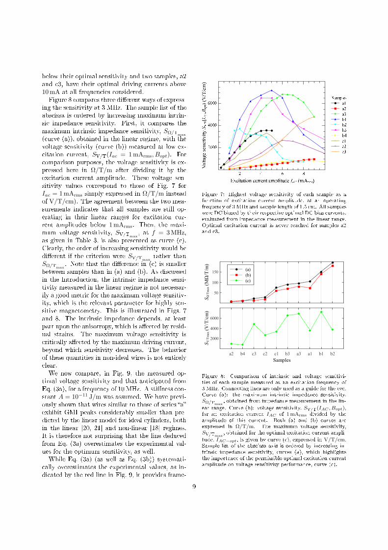
The voltage sensitivity of each sample was mea-sured as described in section 2.4. There might bediculties in GMI measurements, associated withthe reproducibility of electrical contacts and withthe variable mechanical stresses introduced duringthe contact procedure. The maximum RMS valueof the excitation current owing through the wirewas limited to 10 mArms. Note that for some sam-ples the optimal excitation current is greater thanthis value so that the optimal driving current wasnot reached. For such samples the maximum volt-age sensitivity is underestimated.Figure 7 shows the highest voltage sensitivity of

each sample as a function of excitation current am-plitude for an operating frequency of 3 MHz. Atthis frequency, samples a3, b1 and b3 outperformthe others with sensitivities around 7 kV/T/cm,whereas samples a2 and b4 yield relatively poorsensitivity. The optimal driving currents for sam-ples a2 and c3 are clearly higher than the maxi-mum employed in this study. In all cases, intrinsicsensitivity depends upon the operating conditions.A sample will be better or worse than another, de-pending upon the driving current chosen. Any com-parison between specimens which does not properlyaccount for this is rendered less meaningful.The maximum measured voltage sensitivity for

each sample is presented in Table 3 for several fre-quencies. Not surprisingly, the voltage sensitiv-ity increases with frequency. At lower frequencies,sample a3 outperforms the others, but is surpassedby sample b1 at 3MHz. Values in italics corre-spond to those for which the optimal driving cur-rent amplitude is not reached (greater than 10mA).As theoretically expected, this value increases withfrequency. At 10MHz half of the samples operate

8

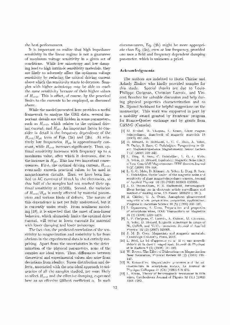
below their optimal sensitivity and two samples, a2and c3, have their optimal driving currents above10mA at all frequencies considered.Figure 8 compares three dierent ways of express-

ing the sensitivity at 3 MHz. The sample list of theabscissa is ordered by increasing maximum intrin-sic impedance sensitivity. First, it compares themaximum intrinsic impedance sensitivity, SΩ/T

max

(curve (a)), obtained in the linear regime, with thevoltage sensitivity (curve (b)) measured at low ex-citation current, SV/T(Iac = 1mArms, Bopt). Forcomparison purposes, the voltage sensitivity is ex-pressed here in Ω/T/m after dividing it by theexcitation current amplitude. These voltage sen-sitivity values correspond to those of Fig. 7 forIac = 1mArms simply expressed in Ω/T/m insteadof V/T/cm). The agreement between the two mea-surements indicates that all samples are still op-erating in their linear ranges for excitation cur-rent amplitudes below 1mArms. Then, the maxi-mum voltage sensitivity, SV/T

max

, at f = 3MHz,as given in Table 3, is also presented as curve (c).Clearly, the order of increasing sensitivity would bedierent if the criterion were SV/T

max

rather thanSΩ/T

max

. Note that the dierence in (c) is smallerbetween samples than in (a) and (b). As discussedin the Introduction, the intrinsic impedance sensi-tivity measured in the linear regime is not necessar-ily a good metric for the maximum voltage sensitiv-ity, which is the relevant parameter for highly sen-sitive magnetometry. This is illustrated in Figs. 7and 8. The intrinsic impedance depends, at leastpart upon the anisotropy, which is aected by resid-ual strains. The maximum voltage sensitivity iscritically aected by the maximum driving current,beyond which sensitivity decreases. The behaviorof these quantities in non-ideal wires is not entirelyclear.We now compare, in Fig. 9, the measured op-

timal voltage sensitivity and that anticipated fromEq. (3a), for a frequency of 10 MHz. A stiness con-stant A = 10−11 J/m was assumed. We have previ-ously shown that wires similar to those of series aexhibit GMI peaks considerably smaller than pre-dicted by the linear model for ideal cylinders, bothin the linear [20, 21] and non-linear [18] regimes.It is therefore not surprising that the line deducedfrom Eq. (3a) overestimates the experimental val-ues for the optimum sensitivity, as well.While Eq. (3a) (as well as Eq. (3b)) systemati-

cally overestimates the experimental values, as in-dicated by the red line in Fig. 9, it provides frame-

Figure 7: Highest voltage sensitivity of each sample as afunction of excitation current amplitude, at an operatingfrequency of 3 MHz and sample length of 1.5 cm. All sampleswere DC biased by their respective optimal DC bias currents,evaluated from impedance measurement in the linear range.Optimal excitation current is never reached for samples a2and c3.

A

BC

DCC

DBCA

EA

FA

FA

CCC

CCC

CCC

E F F FD E D ED E

Figure 8: Comparison of intrinsic and voltage sensitivi-ties of each sample measured at an excitation frequency of3 MHz. Connecting lines are only used as a guide for the eye.Curve (a): the maximum intrinsic impedance sensitivity,SΩ/T

max

, obtained from impedance measurement in the lin-ear range. Curve (b): voltage sensitivity, SV/T(IAC , Bopt),for an excitation current IAC of 1mArms divided by theamplitude of this current. Both (a) and (b) curves areexpressed in Ω/T/m. The maximum voltage sensitivity,SV/T

max

, obtained for the optimal excitation current ampli-tude, IAC−opt, is given by curve (c), expressed in V/T/cm.Sample list of the abscissa axis is ordered by increasing in-trinsic impedance sensitivity, curves (a), which highlightsthe importance of the permissible optimal excitation currentamplitude on voltage sensitivity performance, curve (c).

9

Table 3: Maximum voltage sensitivity obtained for each 1.5 cm long sample, with the corresponding optimal operating con-ditions. Values in italics correspond to those for which the optimal driving current amplitude is not reached (greater than10mA).

Operating frequency 300 kHz 1 MHz 3 MHz 10 MHz

SampleIDC

i SV/Tmax

IAC−opt SV/Tmax

IAC−opt SV/Tmax

IAC−opt SV/Tmax

IAC−opt

mAdc kV/T mArms kV/T mArms kV/T mArms kV/T mArms

a1 0.5 1.03 2 2.76 3 5.37 4.5 6.93 > 10a2 6 0.49 > 10 0.78 > 10 1.47 > 10 1.50 > 10a3 0.5 3.02 3.5 6.84 5 10.26 6 15.2 > 10b1 2 1.58 3 5.40 4 10.81 5 16.27 7b2 0 1.39 1 3.77 1.5 5.57 2 8.91 6b3 2 1.42 3 4.65 4 9.78 5 14.58 6b4 2 0.16 5 0.47 6 1.23 8 4.19 9c1 0 0.80 1.5 1.86 3.5 4.99 4.5 9.67 9c2 0.5 0.47 3 1.35 5 3.99 6 9.29 > 10c3 6 1.27 > 10 3.47 > 10 7.21 > 10 7.99 > 10

iThe optimal DC bias current is deduced from intrinsic impedance sensitivity characterization as discussed in Sec. 2.4.

work for interpreting the data. Based on Eq. (3a),which applies to ideal samples, all CoFe-rich sam-ples (all except a2) have a predicted sensitivityaround 10 to 15 kV/T/cm, with a correspondinglarge spread of measured values. Considering thatthe error bars in the prediction are large, primar-ily due to the uncertainty in the determination ofthe resistivity, and that several samples were notoperated under optimal conditions, it is rather dif-cult to establish a clear trend from this set of data.Using Eq. (3b), which could in principle apply tonon-ideal wires, does not improve the correlation.Indeed, using Gilbert damping parameters deter-mined at 38GHz to predict the response at 10MHzor below is somewhat questionable, as discussed be-low. Finally, both Eqs. (3a) and (3b) predict thatthe sensitivity would be higher in materials withhigher magnetization and resistivity. While thismay partly explain the poor sensitivity of the NiCo-based sample, which has the highest magnetic sus-ceptibility of them all but the lowest Msρ product,this general trend is probably hidden by the eectof inhomogeneity in the samples.

In Fig. 10, we compare the frequency dependenceobserved for SV/T

max

for the three best samples,representative of each fabrication process (a3, b1and c1). The observed sensitivity increases withfrequency, but is always lower, than the ω1/4 de-pendence predicted by (3a) for an ideal wire. Wesuggest that the deviations from ideal wire behav-ior, shown in Figs. 9 and 10, are related to wire de-

fects and imperfections as discussed in Sec. 2.2, inrelation to the approach to saturation. As discussedpreviously [2], the GMI of non-ideal samples can of-ten be modeled using α as an eective frequency de-pendent phenomenological damping parameter in-cluding both intrinsic and extrinsic damping mech-anisms. Such damping is expected to be higherat low frequency (and therefore low applied eld)where the eect of inhomogeneities is the most sig-nicant. The α-values reported in Table 2 weremeasured at 38GHz under applied magnetic eldswhich are three orders of magnitude higher thanthose used at the operating GMI points. As such,they are not necessarily representative of the eec-tive values of α at low eld, but rather indicativeof the potential sensitivity of ideal wires.

5. Discussion and conclusion

The GMI sensitivity of several rapidly solidiedsoft microwires has been studied and analyzed us-ing a simple phenomenological model proposed inRef. [2]. An important objective of our study wasto nd a way of meaningfully comparing wires withdierent radius and exhibiting dierent physicalproperties. We propose that voltage sensitivity perunit length of wire, measured under optimal drivingcurrent, which is directly related to magnetic sensorperformance, is a critical metric to assess the wirepotential for sensitive magnetometry. In this re-spect, we found no evidence permitting us to iden-

10

Figure 9: Comparison of measured and theoretical maximumvoltage sensitivity, SV/T

max

, expressed in kV/T/m, for anexcitation frequency of 10MHz. The red line illustrates amatch between measurement and theory (i.e. measured val-ues are equal to theoretical ones). Sample references areshown for each point and empty symbols are used when theoptimal excitation amplitude is not reached since it is higherthan 10mArms.

Figure 10: Measured maximum voltage sensitivity, expressedin kV/T/m, for samples a3, b1 and c1, as a function of theexcitation frequency, f . Empty symbols are used when theoptimal excitation current amplitude is not reached since itis higher than 10mArms.

tify a sample which greatly surpasses all the oth-ers. Further, the variability of samples from a givensource appears to be comparable with the variabil-ity between sources. In any case, the best samplesstill exhibit sensitivities signicantly below the pre-diction for perfectly cylindrical material with freesurface spins and without defects or nonuniformi-ties. This suggests that no microwires currentlyfabricated approach ideal properties.A methodology based on VSM magnetometry,

ferromagnetic resonance spectroscopy and four-point resistance measurements, has been employedto determine various physical properties enteringinto the model. As highlighted, measurement ofmagnetic moment divided by the sample volumewas found to be unreliable to determine the sat-uration magnetization. Therefore, an alternativeapproach has been proposed. Overall, the physi-cal properties of dierent samples (in some cases,nominally identical), exhibit signicant uctua-tions. Nonetheless, the dispersion of these physicalproperties between samples with similar composi-tions appears to be real, thus opening the ques-tion of the physical uniformity of rapidly solidiedsoft amorphous wires. Despite considerable eortto control these, measurements of intrinsic mag-netoimpedance sensitivity sometimes suer fromproblems of reproducibility of electrical contactsand of mechanical stresses introduced during thecontact procedure. According to the model pre-sented here, change of sensitivity due to uninten-tional stress (induced magnetoelastic anisotropy)can be somewhat compensated by adjusting the op-timal driving current. The reproducibility of elec-trical contacts can also be signicantly improved byelectroplating Cu on the contact zone.As expected from earlier experiments and from

nonlinear modeling [18], there exists an optimumvoltage sensitivity (at a given frequency), at a cur-rent slightly above that at which nonlinear behavioris rst observed. The optimal operating conditionsare specic to each sample (and sensitive to thecontact and stress conditions). When they wereoperated under these conditions, the sensitivity ofthe microwires approached the predictions of themodel more closely and the variability from sampleto sample was considerably reduced. While the fre-quency dependence of optimal sensitivity (Fig. 10)is similar for all samples, the dierences are su-cient to modify the order of sensitivities. In dif-ferent sets of operating conditions (driving currentamplitude and frequency) dierent wires exhibited

11

the best performances.It is important to realize that high impedance

sensitivity in the linear regime is not a guaranteeof maximum voltage sensitivity in a given set ofconditions. While low anisotropy and low damp-ing lead to high intrinsic sensitivity materials, theyare likely to adversely aect the optimum voltagesensitivity by reducing the critical driving currentabove which the sensitivity starts to decrease. Sam-ples with higher anisotropy may be able to reachthe same sensitivity because of their higher valuesof Hcrit. This is oset, of course, by the practicallimits to the currents to be employed, as discussedabove.While the model presented here provides a useful

framework to analyze the GMI data, several im-portant details are still hidden in some parameters,such as Hcrit, which relates to the optimal driv-ing current, and Hpk. An important factor to con-sider in detail is the frequency dependence of theHcrit/Hpk term of Eqs. (3a) and (3b). At rela-tively low frequencies, Hpk is approximately con-stant, while Hcrit increases signicantly. Thus, op-timal sensitivity increases with frequency up to amaximum value, after which it decreases, due tothe increase in Hpk. This has two important conse-quences. First, the optimal driving current, Hcrit,eventually exceeds practical values to be used inmagnetometer circuits. Here, we have been lim-ited to AC currents of 10mA by the electronics, sothat half of the samples had not reached their op-timal sensitivity at 10MHz. Second, the variationof Hcrit/Hpk is surely aected by material param-eters and various kinds of defects. The nature ofthis dependence is not yet fully understood, but itis currently under study. From nonlinear model-ing [18], it is expected that the onset of non-linearbehavior, which ultimately limits the optimal drivecurrent, will occur at lower currents for materialwith lower damping and lower anisotropy.The fact that the predicted correlation of the sen-

sitivity to magnetization and resistivity is far fromobvious in the experimental data is not entirely sur-prising. Apart from the uncertainties in the deter-mination of the physical parameters, none of thesamples are ideal wires. Thus, dierences betweentheoretical and experimental values also arise fromdeviations from ideality. Stress distribution and de-fects, associated with the non-ideal approach to sat-uration of all the samples studied, are most likelyto aect Hcrit and the eective damping, expressedhere as an eective Gilbert coecient α. In such

circumstances, Eq. (3b) might be more appropri-ate than Eq. (3a), even at low frequency, providedone uses a eld and frequency dependent dampingparameter, which is unknown a priori.

Acknowledgments

The authors are indebted to Horia Chiriac andArkady Zhukov who kindly provided samples forthis study. Special thanks are due to Louis-Philippe Carignan, Christian Lacroix, and Vin-cent Boucher for valuable discussion and help dur-ing physical properties characterization and toDr. Djamel Seddaoui for helpful suggestions on themanuscript. This work was supported in part bya mobility award granted by Frontenac programfor France-Quebec exchange and by grants fromCRSNG (Canada).

[1] M. Knobel, M. Vázquez, L. Kraus, Giant magne-toimpedance, Handbook of magnetic materials 15(2003) 497563.

[2] D. Ménard, D. Seddaoui, L. G. C. Melo, A. Yelon,B. Dufay, S. Saez, C. Dolabdjian, Perspectives in Gi-ant Magnetoimpedance Magnetometry, Sensor Letters7 (3) (2009) 339342.

[3] L. Ding, S. Saez, C. Dolabdjian, L. G. C. Melo,A. Yelon, D. Ménard, Equivalent Magnetic Noise Limitof Low-Cost GMI Magnetometer, IEEE Sensors Journal9 (2) (2009) 159168.

[4] L. G. C. Melo, D. Ménard, A. Yelon, L. Ding, S. Saez,C. Dolabdjian, Optimization of the magnetic noise andsensitivity of giant magnetoimpedance sensors, Journalof Applied Physics 103 (3) (2008) 033903033903.

[5] J. O. Strom-Olsen, P. Z. Rudkowski, Ferromagneticbers having use in electronic article surveillance andmethod of making same, US Patent 5003291 (1991).

[6] H. Chiriac, T. A. Óvári, Amorphous glass-coveredmagnetic wires: preparation, properties, applications,Progress in materials Science 40 (5) (1996) 333407.

[7] I. Ogasawara, S. Ueno, Preparation and propertiesof amorphous wires, IEEE Transactions on Magnetics31 (2) (1995) 12191223.

[8] L.-P. Carignan, C. Lacroix, A. Ouimet, M. Ciureanu,A. Yelon, D. Menard, Magnetic anisotropy in arrays ofNi, CoFeB, and Ni/Cu nanowires, Journal of AppliedPhysics 102 (2) (2007) 023905.

[9] J. M. D. Coey, Magnetism and magnetic materials,Cambridge University Press, 2010.

[10] L. Néel, La loi d'approche en a: H et une nouvellethéorie de la dureté magnétique, Journal de Physiqueet le Radium 9 (5) (1948) 184192.

[11] W. Brown, The Eect of Dislocations on MagnetizationNear Saturation, Physical Review 60 (2) (1941) 139147.

[12] H. Kronmüller, Magnetization processes and the mi-crostructure in amorphous metals, Le Journal dePhysique Colloques 41 (C8) (1980) 618625.

[13] L. Kraus, Theory of ferromagnetic resonances in thinwires, Czechoslovak Journal of Physics 32 (11) (1982)12641282.

12

[14] C. Kittel, On the theory of ferromagnetic resonance ab-sorption, Phys. Rev. 73 (2) (1948) 155161.

[15] J. H. Van Vleck, Ferromagnetic resonance, Physica17 (3-4) (1951) 234252.

[16] V. Boucher, D. Ménard, Eective magnetic propertiesof arrays of interacting ferromagnetic wires exhibitinggyromagnetic anisotropy and retardation eects, Phys-ical Review B 81 (17) (2010) 121.

[17] B. Dufay, S. Saez, C. Dolabdjian, D. Seddaoui,A. Yelon, D. Ménard, Improved GMI Sensors UsingStrongly-Coupled Thin Pick-Up Coils, Sensor Letters7 (3) (2009) 334338.

[18] D. Seddaoui, D. Ménard, B. Movaghar, A. Yelon, Non-linear electromagnetic response of ferromagnetic met-als: Magnetoimpedance in microwires, Journal of Ap-plied Physics 105 (8) (2009) 083916.

[19] P. Garoche, A. P. Malozemo, Approach to magneticsaturation in sputtered amorphous lms: Eects ofstructural defects, microscopic anisotropy, and surfaceroughness, Physical Review B 29 (1) (1984) 226231.

[20] D. Ménard, A. Yelon, Theory of longitudinal magne-toimpedance in wires, Journal of Applied Physics 88(2000) 379.

[21] L. G. C. Melo, D. Ménard, P. Ciureanu, A. Yelon, In-uence of surface anisotropy on magnetoimpedance inwires, Journal of applied physics 92 (12) (2002) 72727280.

13