PHYSICAL REVIEW D 024015 (2016) Drivenneutronstarcollapse ...laplace.physics.ubc.ca/Group/Papers/PRD-93-024015-2016.pdf · Here we wish to present work that sets such excited NSs

Driven neutron star collapse: Type I critical phenomena and the initial blackhole mass distribution

Scott C. Noble1,* and Matthew W. Choptuik2,†1Department of Physics and Engineering Physics, The University of Tulsa,

800 South Tucker Drive, Tulsa, Oklahoma 74104, USA2CIFAR Cosmology and Gravity Program, Department of Physics and Astronomy,

University of British Columbia, 6224 Agricultural Road, Vancouver, Canada V6T 1Z1(Received 15 September 2015; published 11 January 2016)

We study the general relativistic collapse of neutron star (NS) models in spherical symmetry. Ourinitially stable models are driven to collapse by the addition of one of two things: an initially ingoingvelocity profile, or a shell of minimally coupled, massless scalar field that falls onto the star. Tolman-Oppenheimer-Volkoff (TOV) solutions with an initially isentropic, gamma-law equation of state serve asour NS models. The initial values of the velocity profile’s amplitude and the star’s central density span aparameter space which we have surveyed extensively and which we find provides a rich picture of thepossible end states of NS collapse. This parameter space survey elucidates the boundary between Type Iand Type II critical behavior in perfect fluids which coincides, on the subcritical side, with the boundarybetween dispersed and bound end states. For our particular model, initial velocity amplitudes greater than0.3c are needed to probe the regime where arbitrarily small black holes can form. In addition, weinvestigate Type I behavior in our system by varying the initial amplitude of the initially imploding scalarfield. In this case we find that the Type I critical solutions resemble TOV solutions on the 1-mode unstablebranch of equilibrium solutions, and that the critical solutions’ frequencies agree well with the fundamentalmode frequencies of the unstable equilibria. Additionally, the critical solution’s scaling exponent is shownto be well approximated by a linear function of the initial star’s central density.

DOI: 10.1103/PhysRevD.93.024015

I. INTRODUCTION

The dynamics of compact gravitating objects out ofequilibrium has always been a topic of much interest inastrophysics. Physical systems that fall under this subjectinclude supernovae, “failed” supernovae such as hyper-novae or collapsars, gamma-ray burst (GRB) progenitors,coalescing binary neutron star (NS) systems, accretingcompact stars, and NSs that undergo sudden phase tran-sitions, to name only a few. In the case of a core collapsesupernova, a NS may form and undergo additional evolu-tion. For instance, the outwardly moving shock wave ofmatter from the supernova may stall and collapse onto thenascent neutron core [1]. In contrast, if the NS is in a binarysystem with a less compact companion star, accretion fromthe companion may push the NS over its Chandrasekharlimit. In either of these cases, the resultant nonequilibriumsystem will most likely undergo a hydrodynamic implosionthat will often result in black hole formation.Here we wish to present work that sets such excited NSs

in the context of critical phenomena in general relativity.Specifically, we wish to investigate (1) the criteria requiredto initiate black hole formation, the boundary betweenblack hole forming scenarios and those that do not form

black holes, and (2) the dynamical behavior of the systemsin general. This paper is one of only several to date thatties critical phenomena to astrophysical scenarios [2–13].We are certainly not the first to study numerical

evolutions of NS models far from equilibrium. For exam-ple, Shapiro and Teukolsky [14] asked whether a stableNS with a mass below the Chandrasekhar mass could bedriven to collapse by compression. With a mixed Euler-Lagrangian code, they began to answer the question bystudying stable stars whose density profiles had been“inflated” in a self-similar manner such that the starsbecame larger and more massive. Due to insufficient centralpressure, such configurations were no longer equilibriumsolutions and inevitably collapsed. By increasing thedegree to which the equilibrium stars were inflated, theywere able to supply more kinetic energy to the system.They found that black holes formed only for stars withmasses greater than the maximum equilibrium mass. Inaddition, Shapiro and Teukolsky studied accretion inducedcollapse, where it was again found that collapse to a blackhole occurred only when the total mass of the system—inthis case the mass of the star and the mass of the accretingmatter—was above the maximum stable mass. Both exam-ples seemed to suggest that even driven stars needed to havemasses above the maximum stable mass in order to produceblack holes. Moreover, they only witnessed three types ofoutcomes: (1) homologous bounce, wherein the entire star

*scott‑[email protected]†[email protected]

PHYSICAL REVIEW D 93, 024015 (2016)

2470-0010=2016=93(2)=024015(23) 024015-1 © 2016 American Physical Society

http://dx.doi.org/10.1103/PhysRevD.93.024015




underwent a bounce after imploding to maximum com-pression; (2) nonhomologous bounce where less than 50%of the matter followed a bounce sequence; and (3) directcollapse to a black hole. Also, Baumgarte et al. [15] using aLagrangian code based on the formulation of Hernandezand Misner [16] qualitatively confirmed these results.In order to investigate the question posed by Shapiro and

Teukolsky further, Gourgoulhon [17,18] used pseudospec-tral methods and realistic, tabulated equations of state tocharacterize the various ways in which a NS may collapsewhen given an ad hoc, polynomial velocity profile. Suchvelocity profiles mimic those seen in core collapse simu-lations as described in [19,20]. Given a sufficiently largeamplitude of the profile, Gourgoulhon was able to formblack holes from stable stars with masses well below themaximum. He was also able to observe bounces off theinner core, but was unable to continue the evolutionsignificantly past the formation of the shock since spectraltechniques typically behave poorly for discontinuoussolutions.To further explore this problem and resolve the shocks

more accurately, Novak [6] used a Eulerian code with high-resolution shock-capturing (HRSC) methods. In addition,he surveyed the parameter space in the black hole–formingregime in much greater detail than previous studies,illuminating a new scenario in which a black hole mayform on the same dynamical time scale as the bounce.Depending on the amplitude of the velocity perturbation,such cases can lead to black holes that have smaller massesthan their progenitor stars. This dependence suggested thatmasses of black holes generated by NS collapse might notbe constrained by the masses of their parents and, con-sequently, could—in principle—allow the black hole mass,MBH, to take on a continuum of values. In addition, inaccordance with the study described in [17], Novak foundthat the initial star did not have to be more massive thanthe maximum mass in order to evolve to a black hole. Infact, he found that for two equations of state—the typicalpolytropic equation of state (EOS) and a realistic EOSdescribed in [21]—arbitrarily small black holes could bemade by tuning the initial amplitude of the velocity profileabout the value at which black holes are first seen. Hence,Novak’s work suggests that black holes born from NSsare able to have masses in the range 0 < MBH ≤ M⋆, whereM⋆ is the mass of the progenitor star. This suggests thatcritical phenomena may play a role in the black hole massfunction of driven NSs.Critical phenomena in general relativity involves

the study of the solutions—called critical solutions—thatlie at the boundary between black hole–forming and blackhole–lacking spacetimes (for reviews please see [22–24]).General relativistic critical phenomena began with a detai-led numerical investigation of the dynamics of a minimallycoupled, massless scalar field in spherical symmetry [25].This first study identified three fundamental features of the

critical behavior: (1) universality and (2) scale invariance ofa critical solution that arises at threshold, with (3) power-law scaling behavior in the vicinity of the threshold. Allthree of these have now been seen in a multitude of collapsemodels with a wide variety of matter sources, includingperfect fluids [26–28], an SU(2) Yang-Mills model [29,30],and collisionless matter [31,32] to cite just a few. It waseventually found that there are two related yet distincttypes of critical phenomena, dubbed Type I and Type II,due to similarities between the critical phenomena obser-ved in gravitational collapse, and those familiar fromstatistical mechanics.Type II behavior entails critical solutions that are either

continuously self-similar (CSS) or discretely self-similar(DSS). Supercritical solutions—those that form blackholes—give rise to black holes with masses, MBHðpÞ, thatscale as a power law,

MBHðpÞ ∝ jp − p⋆jγ; ð1Þ

implying that arbitrarily small black holes can be formed.Here, p parametrizes a 1-parameter family of initial datawith which one can tune toward the critical solution,located at p ¼ p⋆, and γ is the scaling exponent of thecritical behavior. Since MBHðpÞ is, loosely speaking,continuous across p ¼ p⋆, this type of critical behaviorwas named “Type II” since it parallels Type II (continuous)phase transitions in statistical mechanics.As in the statistical mechanical case, there is a Type I

behavior, where the black hole mass “turns on” at a finitevalue. Type I critical solutions are quite different fromtheir Type II counterparts, tending to be metastable starlikesolutions that are either static or periodic. The criticalsolutions can therefore be described by a continuous ordiscrete symmetry in time, analogous to the Type II CSSand DSS solutions. Unlike the Type II case, however, theblack hole masses of supercritical solutions do not follow apower-law scaling. Instead, the span of time, ΔT0ðpÞ—asmeasured by an observer at the origin—that a givensolution is close to the critical solution scales with thesolution’s deviation in parameter space from criticality

ΔT0ðpÞ ∝ −σ ln jp − p⋆j; ð2Þ

where σ is the scaling exponent of Type I behavior.We note that many of the features of critical gravitational

collapse can be understood in a manner that also has aclear parallel in statistical mechanical critical phenomena.In particular, the critical solutions that have been identifiedto date, although unstable, tend to be minimally so in thesense that they have only a single unstable mode inperturbation theory [27,33]. The Lyapunov exponent asso-ciated with this mode can then be directly related to thelifetime-scaling exponent, σ, for Type I solutions, and to themass-scaling exponent, γ, for Type II solutions.

SCOTT C. NOBLE and MATTHEW W. CHOPTUIK PHYSICAL REVIEW D 93, 024015 (2016)

024015-2

In collapse models that involve matter characterized byone or more intrinsic length scales, the possibility of bothtypes of critical behavior arises. Indeed, the boundaryseparating the two types has been studied extensively inthe SU(2) Einstein-Yang-Mills model [29,30] as well as theEinstein-Klein-Gordon system [34]. In the latter case it wasfound that when the length scale λ—which characterizedthe “spatial extent” of a 2-parameter family of initial data—was small compared to the scale set by the massive scalarfield, Type II behavior was observed. The transition fromType II to Type I behavior was calculated for differentfamilies and was found to occur when λm ≈ 1, where m isthe (particle) mass of the scalar field.Two studies particularly close in spirit to our current

work are due to Hawley and Choptuik [35] and Lai andChoptuik [36]. Instead of perturbing TOV solutions [37–39], these authors perturbed stable, spherically symmetric,boson stars. Boson stars are self-gravitating configurationsof a complex scalar field with some prescribed self-interaction (possibly just a mass term), whose only timedependence is a phase that varies linearly with time (see[40] and [41] for reviews). For a given self-interaction, onecan generically construct one-parameter families of bosonstars, where the family parameter can conveniently be takento be the central modulus, ϕð0Þ, of the complex field, andwhich plays the role of the central rest-mass density in TOVsolutions. As with their hydrostatic counterparts (discussedin more detail in Sec. II C), when the total mass,M⋆ðϕð0ÞÞ,of the configurations is plotted as a function of ϕð0Þ, onetypically finds a maximum mass for some ϕð0Þ ¼ ϕmaxð0Þwhich signals a change in dynamical stability: starswith ϕð0Þ < ϕmaxð0Þ are stable, while those with ϕð0Þ >ϕmaxð0Þ are unstable. Additionally, for any family of bosonstars, there is generally a branch of unstable stars—withϕð0Þ ranging from ϕmax to the next value where the massfunction is a local minimum—that have precisely oneunstable mode in perturbation theory. These stars are thuscandidates to be Type I critical solutions in a collapsescenario.Hawley and Choptuik perturbed a boson star by col-

lapsing a spherical pulse of massless scalar field onto itfrom a distance sufficient to ensure that the two matterdistributions were initially nonoverlapping. As such apulse collapses through the origin, the energy distributionsassociated with the two matter fields interact solely throughthe gravitational field. For sufficiently large amplitudesof the scalar field, the resulting increase in curvature withinthe star is enough to significantly compress it, ultimatelyresulting in either black hole formation or a star thatexecutes a sequence of oscillations, often of large ampli-tude. By tuning the initial amplitude of the scalar field,Type I critical solutions were found and, per the aboveobservation, were identified as (perturbed) one-modeunstable boson star configurations. It was verified thatthe lifetimes of near-critical evolutions scaled according to

(2), and that in each case the scaling exponent, σ, wasconsistent with the inverse of the real part of the Lyapunovexponent, ωLy, of the critical solution. Furthermore, valuesof ωLy were independently calculated for several cases byapplying linear perturbation theory to the static boson starbackgrounds, and were shown to be in good agreementwith those measured from the fully dynamical calculations.Finally, since boson stars model many of the characteristicsof TOV solutions, it was conjectured that the observedcritical behavior would carry over to the fluid case.We note that in the results reported in [35] the end state

of marginally subcritical collapse was not identified as aperiodic spacetime (i.e. a perturbed boson star); rather, itwas assumed that the stars would disperse to spatial infinityin such cases. Upon evolving subcritical configurationsfor longer physical times, Lai and Choptuik [36]—in workperformed simultaneously to that of [42]—found that theend states were, in fact, gravitationally bound and oscil-latory. These results were subsequently verified by Hawley[43]. Interestingly, in both studies it was found that duringthe nontrivial gravitational interaction of the masslessscalar field and the boson star there was a transfer of massenergy from the massless scalar field to the complex scalarfield, resulting in an increase of the gravitating mass of theboson star.Returning now to the fluid case, Siebel et al. [44] sought

to measure the maximum NS mass allowed by the presenceof a perturbing pulse of minimally coupled, masslessscalar field. A general relativistic hydrodynamic code usinga characteristic formulation was used to investigate thespherically symmetric system. However, instead of varyingthe massless scalar field they studied five distinct starsolutions having a range of central densities that straddledthe threshold of black hole formation. They found that theperturbation either led to a black hole or to oscillations ofthe star about its initial configuration. Further, in order totest their new three-dimensional general relativistic fluidcode, Font et al. [45] dynamically calculated the funda-mental and harmonic mode frequencies of spherical TOVsolutions. They observed the transition of a TOV solutionon the unstable branch to the stable branch by evolving anunstable solution that was perturbed at the truncation errorlevel. The unstable star overshot and then oscillated aboutthe stable solution, contradicting a common assumption inthe field that stars from the unstable branch always formedblack holes. Evolving from initial conditions consistingof an unstable TOV star has continued to be used forcode-testing purposes [46]. Liebling et al. [9,12] performeda similar study with weakly magnetized unstable TOVsolutions in 3-d, but employed explicit and tunable per-turbations to the pressure/density—as well as—a tunableminimally-coupled scalar field. They, too, found evidencefor Type I behavior, and were able to tune close to thethreshold (to within 10−6) and demonstrate the expectedscaling behavior with the scalar field perturber. All the

DRIVEN NEUTRON STAR COLLAPSE: TYPE I CRITICAL … PHYSICAL REVIEW D 93, 024015 (2016)

024015-3

different kinds of perturbations they employed drove thesystem to the same, seemingly universal solution.Proximity to the critical threshold was improved in [10],wherein they perturbed axisymmetric unstable TOV starsby truncation error and a small ingoing velocity distribu-tion, while tuning with the central density of the star.Apart from thework presented here (and in [42]), themost

exhaustive explorations of Type I behavior involving NSsare that of Jin and Suen [7], Wan et al. [8,47,48], andKellerman, Radice, and Rezzolla [11]. The results presentedin these papers indicated that the head-on axisymmetriccollision of twoNSs can be tunedwith a variety of initial dataparameters to a critical threshold that bifurcates end statesinvolving either a single black hole or a single more massiveoscillating NS. Universality of the critical behavior wassupported by tuning separately the initial magnitude of thestellar velocities, central densities and adiabatic index oftheir polytropic EOS. Threshold solutions were found tohigh precision for all three of the tuning variables. Allthreshold solutions were found to be perturbed TOVsolutions on the unstable branch, no matter the tuningparameter. Since changes in the adiabatic index may mimicthe effects of cooling and accretion, an interesting conjecturewas made that critical behavior might be realizable withoutthe need for fine-tuning [7]. Further, frequencies at whichthe near-threshold solution oscillated were measured andfound to differ—by 1 to 2 orders of magnitude—from thefrequencies of the l ¼ 0, 1 perturbation modes about theinitial stable TOV solution [8]. The seeming discrepancy infrequencies was eventually explained by [11] when theydemonstrated that the near-threshold solutions were per-turbed TOV solutions on the unstable branch, and that theoscillations occurred at the fundamental mode of theunstable TOV solution—not the original stable TOV sol-ution. This realization in the literature paralleled conclusionsmade years before in the boson star context [36], and in theTOV context [42].In this paper, we investigate both types of critical behavior

using a perfect fluid model, although we focus for the mostpart on the Type I case. For the first timewith TOV solutions,we demonstrate that the scaling exponent, σ, is consistentwith the inverse of the real part of the Lyapunov exponent,ωLy, of the critical solution. This provides further evidenceto support the notion that the Type I critical solutions areperturbed TOV solutions on the unstable branch. The initialconditions which we adjust entail a stable TOV star with thestiffest causal polytropic EOS (Γ ¼ 2), plus some sort of“perturbing agent.”Themethods bywhichwedrive a star to anonequilibrium state involve: (1) giving the star an initiallyingoing velocity profile, and (2) collapsing a sphericalshell of scalar field onto it. Neither method can be consideredtruly perturbative since both can drive the star to totalobliteration or prompt collapse to a black hole, but we usethis term since a better one is lacking.Section II provides the theory describing our systems

and the numerical methods we use to simulate them. In

Sec. IV, we begin our study of stellar collapse by exten-sively covering the parameter space of initial conditionsfor velocity-perturbed stars. The results from this sectionprovide a broad view of the range of dynamical scenariosone can expect in the catastrophic collapse of NSs. We thenemploy this knowledge in our examination of the solutionsthat lie on the verge of black hole formation. Both Type Iand Type II solutions are found. The stars’ Type I criticalbehavior is explored in Sec. V (their Type II behavior hasbeen investigated in a related paper [49]). The thresholdsolutions we calculate from the Type I study are thencompared to unstable TOV solutions. In addition, for thefirst time, a parameter-space boundary separating the twotypes of phenomena is identified and discussed. Finally,we conclude in Sec. VI with some closing remarks andnotes on possible future work.

II. THEORETICAL MODEL

The equations and methods employed in this studyclosely follow those used in [49]. The primary differenceis that we sometimes use a massless scalar field that isminimally coupled to gravity, and hence to the fluid. Werefer the reader to [49] for details regarding the evolution ofthe hydrodynamics equations, but give here the equationsthat describe this “fluidþ scalar” system and the methodsused to evolve the scalar field.

A. The geometry equations

We largely follow the notation established in our pre-vious paper onType II collapse of a perfect fluid [49].We usegeometrized units such that G ¼ c ¼ 1, and tensor notationand sign conventions that followWald [50].When coordinatebases are explicitly used, Greek and Roman indices willrefer to spacetime and purely spatial components, respec-tively (i.e. μ; ν;… ∈ f0; 1; 2; 3g, and i; j; k ∈ f1; 2; 3g).Quantities in boldface, e.g. q; f, are generally state vectors.As in many previous critical phenomena studies in

spherical symmetry [6,25,26,28,29], we employ the so-called polar-areal metric

ds2 ¼ −αðr; tÞ2dt2 þ aðr; tÞ2dr2 þ r2dΩ2: ð3ÞSince we will use a variety of sources in this study, we statethe equations governing the metric functions using theformulation of Arnowitt, Deser and Misner (ADM) [51]and no specific assumption about the precise form of stress-energy tensor. To update a at each time step, we solve theHamiltonian constraint,

a0

a¼ 4πra2ϱþ 1

2rð1 − a2Þ; ð4Þ

where ϱ is the local energy density measured by anobserver moving orthonormal to the spacelike hypersurfa-ces. Note that a “prime” will denote differentiation withrespect to r and a “dot” will represent differentiation with


024015-4

respect to t. In our coordinate basis, the 4-velocity, na, ofthis orthonormal observer has components

nμ ¼h1α; 0; 0; 0

iT: ð5Þ

Hence, ϱ can be shown to be

ϱ ¼ Tμνnμnν ¼ Ttt=α2: ð6ÞThe lapse function α is calculated at each step via the polarslicing condition,

α0

α¼ a0

aþ 1

rða2 − 1Þ − 8πa2

r

�Tθθ −

r2

2ðTi

i − ϱÞ�: ð7Þ

Even though it is used solely for diagnostic purposes, westate here for completeness the momentum constraint,which yields an evolution equation for a,

_a ¼ −4πrαajr; ð8Þwhere jr is the only nonvanishing component of themomentum density measured by the orthonormal observer,

ja ≡ ðgac þ nancÞnbTbc: ð9ÞFor diagnostic purposes, it is convenient to introduce themass aspect function, m, given by

mðr; tÞ≡ r2

�1 −

1

a2

�: ð10Þ

We note that polar-areal coordinates cannot penetrateapparent horizons, but that the formation of a blackhole in a given calculation is nonetheless signaled by2mðt; ~rÞ=~r → 1, for some specific radial coordinate, r ¼ ~r.

B. The matter equations

We model NS matter as a perfect fluid. Modernconservative methods that utilize the characteristic structureof the fluid equations of motion expressed in conservativeform have been very successful in evolving highly rela-tivistic flows in the presence of strong gravitational fields(see [45,52–55] for a small but representative selection ofpapers on this topic), and we follow that approach here. Inparticular, we use a formulation used by Romero et al. [55]and a change of variables similar to that performed byNeilsen and Choptuik [54].One way in which we drive NSmodels to collapse entails

the inclusion of a massless scalar field which dynamicallyperturbs the star. We also use a driving mechanism thatinvolves no scalar field. Not surprisingly, it turns outthat the equations governing the geometry and fluidequations in the “fluid-only” system can be recoveredfrom those in the fluidþ scalar system simply by settingthe scalar field, ϕðr; tÞ, to zero for all r and t. Hence,our numerical implementation always uses the full

fluidþ scalar equations for determining fluid and geo-metric fields: if we wish to include the scalar field, wesimply initialize it to a nonzero value and evolve it intandem with the fluid. Thus, by stating the fluid equationsof motion (EOM) for the fluidþ scalar system, we arealso simultaneously—yet indirectly—stating them in thefluid-only system.The EOM for the two matter sources are derived, in part,

from the local conservation of energy

∇aTab ¼ 0; ð11Þ

where Tab is the total stress-energy tensor. Since there is noexplicit coupling between the two matter sources, the totalstress tensor is a sum of the stress tensors of the individualsources

Tab ¼ ~Tab þ T̂ab; ð12Þwhere T̂ab and ~Tab are the stress-energy tensors of the fluidand scalar field, respectively. Further, the local conserva-tion of energy equation holds separately for each stress-energy. Specifically,

∇aTab ¼ ∇a ~Tab ¼ ∇aT̂ab ¼ 0: ð13ÞThe scalar field stress-energy tensor is

~Tab ¼ ∇aϕ∇bϕ −1

2gabð∇cϕ∇cϕþ 2VðϕÞÞ; ð14Þ

where VðϕÞ is the scalar potential. In the followingequations, we will assume that VðϕÞ is nonzero, however,we have set VðϕÞ≡ 0 in all of the calculations reportedbelow. Since there is no direct interaction between thescalar field and the fluid, (13) yields the usual equation ofmotion for the scalar field:

□ϕ≡∇a∇aϕ ¼ ∂ϕVðϕÞ: ð15ÞWe can convert this to a system of first-order (in time)PDEs by introducing auxiliary variables, Ξ and ϒ, definedby

Ξ≡ ϕ0; ϒ≡ aα_ϕ: ð16Þ

With these definitions the EOM become

_Ξ ¼ ðXϒÞ0; ð17Þ

_ϒ ¼ 1

r2ðr2XΞÞ0 − αa∂ϕV; ð18Þ

where X ≡ α=a.The fluid equations of motion can be easily derived from

the definition of the perfect fluid stress-energy tensor,

T̂ab ¼ ðρþ PÞuaub þ Pgab; ð19Þ


024015-5

the local conservation of energy equation (13) and the localconservation of baryon number

∇aðρ∘uaÞ ¼ 0: ð20ÞHere, ua is the 4-velocity of a given fluid element, P is theisotropic pressure, ρ ¼ ρ∘ð1þ ϵÞ is the energy density, ρ∘ isthe rest-mass energy density, and ϵ is the specific internalenergy. Instead of the 4-velocity of the fluid, a more usefulquantity is the radial component of the Eulerian velocity ofthe fluid as measured by a Eulerian observer:

v ¼ aur

αut; ð21Þ

where uμ ¼ ½ut; ur; 0; 0� (recall that we are working inspherical symmetry). The associated “Lorentz gammafunction” is defined by

W ¼ αut: ð22ÞGiven the fact that the 4-velocity is timelike and unitnormalized, i.e. uμuμ ¼ −1, v and W are related by

W2 ¼ 1

1 − v2: ð23Þ

In conservation form, the fluid’s EOM are

∂tqþ 1

r2∂rðr2XfÞ ¼ ψ; ð24Þ

where the state vector q is a vector of conserved variables,and f and ψ are—respectively—the flux and source statevectors. Our choice of conserved variables follows that ofNeilsen and Choptuik [54], and leads to improved accuracyin the ultrarelativistic regime (ρ ≫ ρ0):

q ¼

264D

ΠΦ

375; f ¼

24

Dv

vðΠþ PÞ þ P

vðΦþ PÞ − P

35; ψ ¼

264

0

Σ−Σ

375;

ð25Þ

where

D ¼ aρ∘W; ð26Þ

Π ¼ E −Dþ S; ð27Þ

Φ ¼ E −D − S; ð28Þ

S ¼ ρ∘hW2v; ð29Þ

E ¼ ρ∘hW2 − P; ð30Þ

h≡ 1þ ϵþ P=ρ∘ is the specific enthalpy of the fluid, D isthe Eulerian rest-mass density, and Π and Φ are linearcombinations of the Eulerian momentum density (S) and

internal energy density (E −D). We use P, ρ∘, and v asprimitive variables. For the sake of efficiency, we state thesource function, Σ, in terms of derivatives of the metricfunctions so that additional matter sources can be incorpo-rated into the model more easily:

Σ≡ Θþ 2PXr

ð31Þand

Θ ¼ −2_aSa

−α0

αXE −

a0

aXðSvþ PÞ: ð32Þ

In practice, we use a simplified form of Θ derived fromthe constraints (4) and (8) and the slicing condition (7)to eliminate a0, α0 and _a. However, this requires knowledgeof the full stress-energy tensor, Tab, not just the fluid’sstress-energy tensor, T̂ab, to calculate. In the fluidþ scalarsystem,

Θ ¼ αa

�ðSv − EÞ

�4πrð2P − VðϕÞÞ þ m

r2

�

þ P

�mr2

− 4πrVðϕÞ��

− 2πrX½4ΞϒSþ ðΞ2 þϒ2ÞðSvþ Pþ EÞ�: ð33ÞWhen following the gravitational interaction between

the fluid and scalar field, particularly interesting quan-tities to track are the two contributions to dm=dr:

dmdr

¼ 4πr2ϱ ¼ 4πr2ϱfluid þ 4πr2ϱscalar; ð34Þ

dmfluid

dr¼ 4πr2E; ð35Þ

dmscalar

dr¼ 4πr2

�1

2a2ðΞ2 þϒ2Þ þ VðϕÞ

�: ð36Þ

However, the two mass contributions can only be unam-biguously differentiated in regions of nonoverlappingsupport, since—for instance—∂mscalar=∂r depends onmetric quantities which in turn depend on the local energycontent of all matter distributions that are present. We notethat expressing dm

dr in the form of Eq. (34) is possiblebecause of our particular gauge choice.The EOS closes the system of hydrodynamic equations.

Because of the extensive nature of our parameter spacesurvey, we wish to restrict ourselves to closed-form(i.e. nontabulated) state equations. For isentropic flows,the polytropic EOS,

P ¼ KρΓ∘ ; ð37Þfor some constant, K, and adiabatic index, Γ, is commonlyused. In addition, we use the “ideal-gas” or “gamma-law”EOS


024015-6

P ¼ ðΓ − 1Þρ∘ϵ: ð38ÞOur initial NS models are solutions to the sphericallysymmetric hydrostatic Einstein equations, and are com-monly known as Tolman-Oppenheimer-Volkoff (TOV)solutions [37,39]. We use both EOSs (38) and (37) toset the initial data, but use only the ideal-gas EOS (38) toevolve any specific configuration [56]. To simulate stiffmatter at supernuclear densities—characteristic of neutronstars—we use Γ ¼ 2 in all of the calculations describedbelow. We also note that, as pointed out by Cook et al. [58],the constant K can be thought of as the fundamental lengthscale of the system, which one can use to scale anydynamical quantity with values of ðK;ΓÞ to a system withdifferent values ðK0;Γ0Þ. As with G and c, we set K ¼ 1.This makes our equations unitless, ensuring that ourdynamical variables are not at arbitrarily different ordersof magnitude, and, as discussed in Appendix A, expeditingthe transformation of results to another set of ðK;ΓÞ.In summary, in our simulations of self-gravitating,

ideal-gas fluids, the fluid is evolved by solving (24) and(25), the scalar field is evolved using (17) and (18), whilethe geometry is simultaneously calculated using theHamiltonian constraint (4) and the slicing condition (7).The specific methods we employ to numerically integratethese equations are briefly explained in Sec. III.

C. Initial star solutions

Since the TOV equations take the form of a coupled setof ordinary differential equations, their solution does notgenerally require the use of sophisticated numerical meth-ods. Readers who are interested in more details are referredto the pseudocode description in Shapiro and Teukolsky[57], as well as the discussion of our specific approachgiven in [42].Analysis of TOV solutions has a rich history [59] which

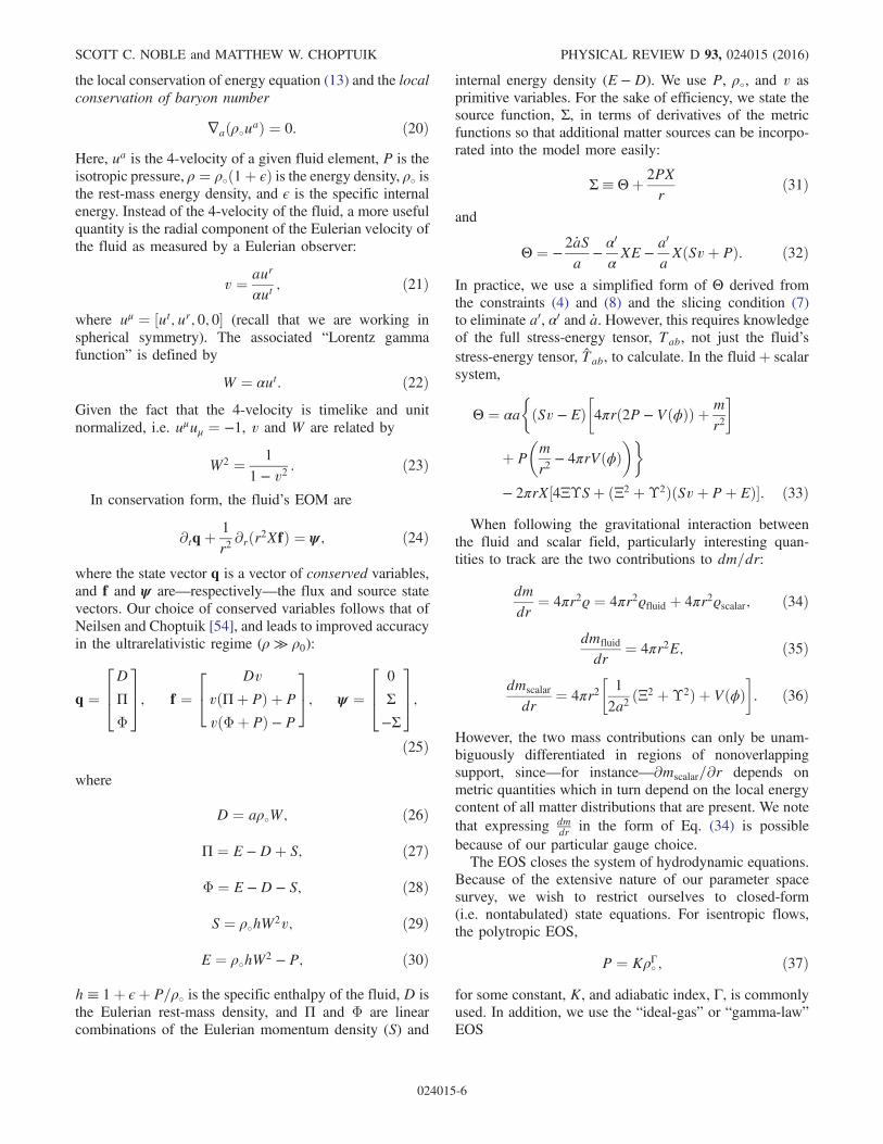
we will not discuss here. We do, however, wish to noteone important aspect of such solutions that is crucial tounderstanding their role in Type I critical behavior, andwhich has already been touched upon in the Introductionin the context of boson stars. Given an EOS, the TOVsolutions can be parametrized by their central pressures;in our case, the EOS (37) allows us to reparametrize thesolutions with respect to the central rest-mass density, ρc.Arguments from linear stability analysis [59] tell us thatTOV solutions with the smallest central densities are stableto small perturbations, while those solutions with ρc at theopposite end of the spectrum (large ρc) are unstable. A plotofM⋆ðR⋆Þ is shown in Fig. 1, where R⋆ is the radius of thestar and we see that M⋆ðR⋆Þ winds up with increasingcentral density. At the global maximum of M⋆ðR⋆Þ thefundamental, or lowest, mode becomes unstable. After eachsubsequent local extremum in the direction of increasingρc, the next lowest mode becomes unstable. For instance,there are four local extrema of M⋆ðR⋆Þ shown in Fig. 1, so

those solutions with the largest ρc will have their fourlowest modes exponentially grow in time.As discussed previously, black hole critical solutions are

typically characterized by a single growing mode. Hence,the Type I behavior associated with “perturbed” TOVsolutions can be immediately anticipated to entail thoseTOV solutions that lie between the first and second extremaof M⋆ðρcÞ. For subsequent reference we note that with theunits and EOS that we have adopted, the most massivestable TOV solution has a central density ρc ≃ 0.318 and amass M⋆ ≃ 0.1637.After the initial, starlike solution is calculated, an

ingoing velocity profile is sometimes added to drive thestar to collapse. In order to do this, we follow theprescription used in [17] and [6]. The method describedtherein involves specifying the coordinate velocity,

U≡ drdt

¼ ur

ut; ð39Þ

of the star, and then finding the Eulerian velocity, v, oncethe geometry has been calculated. In general, the profiletakes the algebraic form

UðxÞ ¼ A0ðx3 − B0xÞ: ð40ÞThe two profiles that were used in [6] are

U1ðxÞ ¼U∘2ðx3 − 3xÞ;

U2ðxÞ ¼27U∘10

ffiffiffi5

p�x3 −

5x3

�; ð41Þ

where x≡ r=R⋆. Unless stated otherwise, U1 will be usedfor all the results herein.

FIG. 1. Mass versus radius of TOV solutions using Γ ¼ 2 andK ¼ 1 with the polytropic EOS (37). In the inset, we show adetailed view of the spiraling behavior. The arrow along the rightside of the curve indicates the direction of increasing centraldensity.


024015-7

Specifying the coordinate velocity instead of v compli-cates the computation of the metric functions at t ¼ 0.Our method for dealing with this difficulty is describedin Appendix B.

III. NUMERICAL TECHNIQUES

Simulating the highly relativistic flows encountered in thedriven collapse of NSs entails solving a system of coupled,partial and ordinary differential equations that describe howthe fluid, scalar field, and gravitational field evolve in time.High-resolution shock-capturing methods are used to evolvethe fluid and the iterative crank Nicholson method, withsecond-order spatial differences, is used for the scalar field.Both methods are second-order accurate, except that thefluid method is first-order accurate near shocks and at localextrema. The rapid numerical prototyping language (RNPL)written byMarsa and Choptuik [60] is used to handle check-pointing, input/output, and memory management for all oursimulations; we do not use the language of RNPL itself forour finite differencing, but use original, secondary routinesthat are called from the primary RNPL routines.More detailsof the code, along with descriptions of code tests can befound in [42,49].

IV. VELOCITY-INDUCED NEUTRONSTAR COLLAPSE

Here we present a description of the various dynamicscenarios we have seen in perturbed NS models, as afunction of the initial star solution and the magnitude of theinitial velocity profile. These results are compared to thosefrom previous studies—most notably that of Novak [6]—but also provide some new insights. Specifically, thissection provides a description of various phases we haveidentified in parameter space, including those from a surveyof the subcritical regime that is more detailed than hasbeen reported in prior work. In Sec. V we then focus onthe critical phenomena observed at the threshold of blackhole formation, and where collapse is induced via inter-action of the fluid star with a collapsing pulse of masslessscalar field.In this section any specific TOV solution is driven out

of equilibrium by endowing it with an ingoing profile forthe initial coordinate velocity, Uðr; 0Þ, as described inSec. II C. We measure the magnitude of this perturbation bythe absolute value of the minimum value of the Eulerianvelocity v, vmin, at the initial time. We find that vmin isuniquely specified by the parameter U∘ provided thatwe follow the prescription for generating perturbed TOVstars given in Appendix B. We also note that vmin is a morephysical quantity than similar parameters—e.g. U∘—thatpertain to the fluid’s gauge-dependent, coordinate velocity.Our survey used 22 different stable TOV solutions—

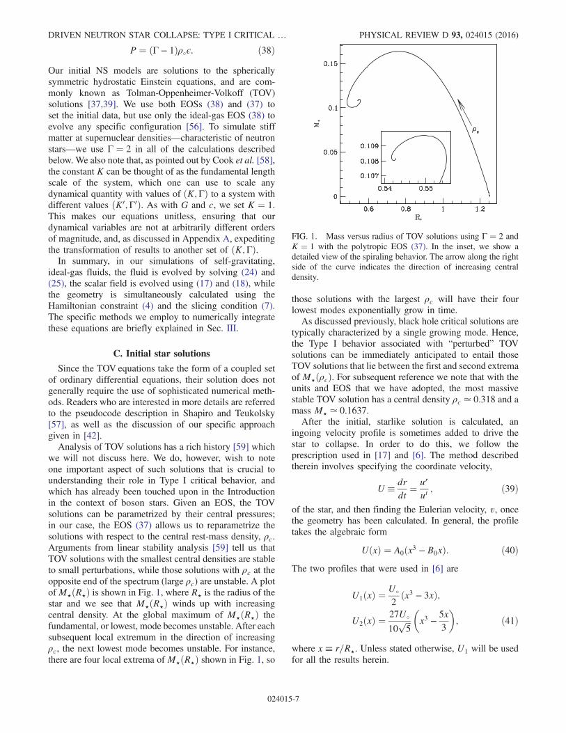
specified by the initial central density ρc—shown in Fig. 2.The solutions used for the parameter space survey are

displayed along the M⋆ðρcÞ curve for Γ ¼ 2 TOV solu-tions. We note that a wide spectrum of stars were chosen,from noncompact stars that are relatively large and diffuse,to compact and dense stars.By sampling vmin and the initial central density of the star,

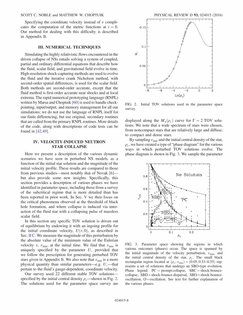
ρc, we have created a type of “phase diagram” for the variousways in which perturbed TOV solutions evolve. Thephase diagram is shown in Fig. 3. We sample the parameter

FIG. 2. Initial TOV solutions used in the parameter spacesurvey.

FIG. 3. Parameter space showing the regions in whichvarious outcomes (phases) occur. The space is spanned bythe initial magnitude of the velocity perturbation, vmin, andthe initial central density of the star, ρc. The small blackrectangular region located at ðρc; vminÞ ∼ ð0.05; 0.53–0.55Þ rep-resents a set of solutions that undergo an SBO-type evolution.Phase legend: PC ¼ prompt collapse, SBC¼ shock-bounce-collapse, SBD¼shock-bounce-dispersal, SBO¼shock-bounce-oscillation, O¼oscillation. See text for further explanation ofthe various phases.


024015-8

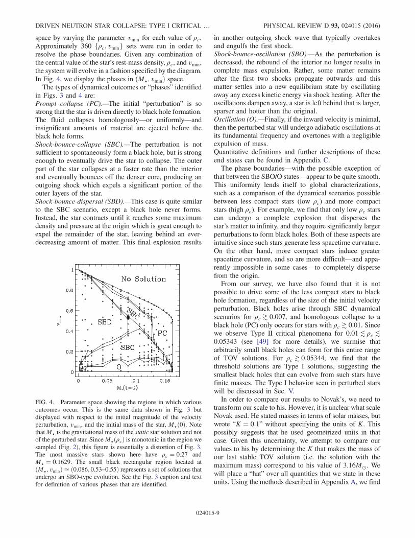
space by varying the parameter vmin for each value of ρc.Approximately 360 fρc; vming sets were run in order toresolve the phase boundaries. Given any combination ofthe central value of the star’s rest-mass density, ρc, and vmin,the system will evolve in a fashion specified by the diagram.In Fig. 4, we display the phases in ðM⋆; vminÞ space.The types of dynamical outcomes or “phases” identified

in Figs. 3 and 4 are:Prompt collapse (PC).—The initial “perturbation” is sostrong that the star is driven directly to black hole formation.The fluid collapses homologously—or uniformly—andinsignificant amounts of material are ejected before theblack hole forms.Shock-bounce-collapse (SBC).—The perturbation is notsufficient to spontaneously form a black hole, but is strongenough to eventually drive the star to collapse. The outerpart of the star collapses at a faster rate than the interiorand eventually bounces off the denser core, producing anoutgoing shock which expels a significant portion of theouter layers of the star.Shock-bounce-dispersal (SBD).—This case is quite similarto the SBC scenario, except a black hole never forms.Instead, the star contracts until it reaches some maximumdensity and pressure at the origin which is great enough toexpel the remainder of the star, leaving behind an ever-decreasing amount of matter. This final explosion results

in another outgoing shock wave that typically overtakesand engulfs the first shock.Shock-bounce-oscillation (SBO).—As the perturbation isdecreased, the rebound of the interior no longer results incomplete mass expulsion. Rather, some matter remainsafter the first two shocks propagate outwards and thismatter settles into a new equilibrium state by oscillatingaway any excess kinetic energy via shock heating. After theoscillations dampen away, a star is left behind that is larger,sparser and hotter than the original.Oscillation (O).—Finally, if the inward velocity is minimal,then the perturbed star will undergo adiabatic oscillations atits fundamental frequency and overtones with a negligibleexpulsion of mass.Quantitative definitions and further descriptions of theseend states can be found in Appendix C.The phase boundaries—with the possible exception of

that between the SBO/O states—appear to be quite smooth.This uniformity lends itself to global characterizations,such as a comparison of the dynamical scenarios possiblebetween less compact stars (low ρc) and more compactstars (high ρc). For example, we find that only low ρc starscan undergo a complete explosion that disperses thestar’s matter to infinity, and they require significantly largerperturbations to form black holes. Both of these aspects areintuitive since such stars generate less spacetime curvature.On the other hand, more compact stars induce greaterspacetime curvature, and so are more difficult—and appa-rently impossible in some cases—to completely dispersefrom the origin.From our survey, we have also found that it is not

possible to drive some of the less compact stars to blackhole formation, regardless of the size of the initial velocityperturbation. Black holes arise through SBC dynamicalscenarios for ρc ≳ 0.007, and homologous collapse to ablack hole (PC) only occurs for stars with ρc ≳ 0.01. Sincewe observe Type II critical phenomena for 0.01≲ ρc ≲0.05343 (see [49] for more details), we surmise thatarbitrarily small black holes can form for this entire rangeof TOV solutions. For ρc ≳ 0.05344, we find that thethreshold solutions are Type I solutions, suggesting thesmallest black holes that can evolve from such stars havefinite masses. The Type I behavior seen in perturbed starswill be discussed in Sec. V.In order to compare our results to Novak’s, we need to

transform our scale to his. However, it is unclear what scaleNovak used. He stated masses in terms of solar masses, butwrote “K ¼ 0.1” without specifying the units of K. Thispossibly suggests that he used geometrized units in thatcase. Given this uncertainty, we attempt to compare ourvalues to his by determining the K that makes the mass ofour last stable TOV solution (i.e. the solution with themaximum mass) correspond to his value of 3.16M⊙. Wewill place a “hat” over all quantities that we state in theseunits. Using the methods described in Appendix A, we find

FIG. 4. Parameter space showing the regions in which variousoutcomes occur. This is the same data shown in Fig. 3 butdisplayed with respect to the initial magnitude of the velocityperturbation, vmin, and the initial mass of the star, M⋆ð0Þ. NotethatM⋆ is the gravitational mass of the static star solution and notof the perturbed star. SinceM⋆ðρcÞ is monotonic in the region wesampled (Fig. 2), this figure is essentially a distortion of Fig. 3.The most massive stars shown here have ρc ¼ 0.27 andM⋆ ¼ 0.1629. The small black rectangular region located atðM⋆; vminÞ≃ ð0.086; 0.53–0.55Þ represents a set of solutions thatundergo an SBO-type evolution. See the Fig. 3 caption and textfor definition of various phases that are identified.


024015-9

that this factor of K is K̂ ¼ 5.42 × 105 cm5 g−1 s−2. LetM1

be the mass of the least massive star that can form a blackhole through any scenario, and M2 be the mass of the leastmassive star that we observe to undergo prompt collapseto a black hole. In our units, we find M1 ≃ 0.01656 atρc ¼ 0.007, and M2 ≃ 0.02309 at ρc ¼ 0.01. Using K̂ toconvert our masses to his yields M̂1 ¼ 0.320M⊙ versusM̂1 ¼ 1.155M⊙, and M̂2 ¼ 0.446M⊙ where Novak reportsM̂2 ≈ 2.3M⊙. Note that M̂2 is estimated from Fig. 5 of [6],where a velocity profile equivalent to our U2 profile (41) isused. Since we have only performed the parameter spacesurvey for U1 we cannot say what we would get for M2

when using U2. However, Novak performed a comparisonbetween these two profiles and found that his estimatesfor M1 deviated by about 1% between the two. Hence, webelieve it is adequate to quote his result for U2 in order tocompare to our result for U1.The difference in masses is also obvious in our res-

pective phase diagrams from the parameter space surveys,where the point along the ρc axis (nB in Novak’s case)at which black holes can form occurs for noticeablymore compact stars in Novak’s case [61]. Another signifi-cant distinction we see in our phase space plot is anabsence of SBC states for larger ρc. Novak seems toobserve such scenarios all the way to the turnover point(ρc ¼ 0.318), whereas we find that they no longer happenfor ρc ≳ 0.108.Additionally, we believe our study is the first to

extensively cover the subcritical region of NS collapse.While the method by which the NSs are perturbed may notbe the most physically relevant prescription, we are able tosee all the collapse scenarios found in previous works.Much of the previous research focused on compact starsnear the turnover point or studied some other regionexclusively (e.g. [44,45,55,62,63]), while others individu-ally observed much of the phenomenon without thoroughlyscrutinizing the boundaries between the phases [6,14,17].Our parameter space survey also sheds light on the

critical behavior observed at the threshold of black holeformation. Specifically, we see that the SBD/SBO boun-dary on the subcritical side of the diagram seems to becorrelated with the transition from Type II to Type I criticalbehavior. The Type II threshold lies along the SBD/SBCboundary, while the Type I threshold occurs along the linethat separates SBO and O cases from black hole–formingcases. We have been able to determine that ρc ≈ 0.05344 isthe approximate point at which the transition from Type IIto Type I behavior occurs. For Type II minimally subcriticalsolutions near this transition, the matter disperses from theorigin but it is difficult to say if it escapes to infinity sinceour grid refinement procedure is incapable of coarseningthe domain. Consequently, the time step is too small toallow for longtime evolutions of these dispersal cases, andwe are unable to guarantee that they do indeed disperseto infinity. In addition, the self-similar portion of these

marginally subcritical solutions entails only a small amountof the original star’s matter, the remainder of which could,in principle, collapse into a black hole at a time after theinner self-similar component departs from the origin.Hence, with our current code, it is difficult to determinethe ultimate fate of these dispersal scenarios.What does this parameter survey suggest about the black

hole mass function from driven NS collapse? For PCscenarios, the black hole mass is approximately the sameas the progenitor star’s mass. The SBC/PC boundary markswhere the black hole mass function can begin to signifi-cantly deviate from the stellar mass function. The leastextreme (smallest vmin) SBC scenario takes place nearvmin ≃ 0.3, ρc ≃ 0.1 and M⋆ ≃ 0.13. Such a large velocityprofile may seem unphysical, however, a self-consistent,general relativistic simulation of a core collapse supernovain spherical symmetry performed by Liebendörfer et al.[64] led to a minimum velocity of ∼ − 0.6c soon afterbounce. This suggests that vmin ≳ 0.3 is not so unrealistic.Also, it means that Type II behavior may be physicallyattainable in nature if—in fact—vmin reaches the magni-tudes seen in [64] since vmin ≃ 0.55 is the smallest velocityprofile that leads to Type II behavior. However, we find thatMBH becomes a power law onlywhen vmin has been tuned toless than 0.01% of the critical value [49], suggesting thatsuch cases will not affect the black hole mass functionsignificantly. Unfortunately, we have not measured thedependence of MBH on vmin and ρc in the SBC regime,and—therefore—are not sure if the distribution is nontrivial.We hope to measure this in the future.Wan et al. [8] present a similar phase space survey of a

head-on collision between two identical Gaussian distri-butions of stiff matter (Γ ¼ 2) to approximate the head-onmerger of identical neutron stars. The two Gaussiandistributions were boosted toward each other with thesame velocity magnitude. The amplitude of the boostvelocities and the initial central densities of the Gaussiandistributions were varied to explore the nature of the criticalsurface. As the central densities were varied, the totalbaryonic masses of the pulses were kept constant byadjusting the width of each distribution. Like us, they findthat there is a line that separates black hole forming initialconditions from NS forming conditions. Unlike our results,however, they find that their line is concave leftward,suggesting that there is a maximum density beyond whichblack hole formation is impossible independent of boostvelocity. Further, it suggests that at a given initial centraldensity (below this upper limit) there are two criticaltransitions: from NS-forming to BH-forming to NS-forming—i.e. there is a velocity value above which onlyNS formation is possible. Wan [48] explains further that thesecond threshold arises because at this point the mergerproduces a shock that heats the gas to the point that collapseis prevented. In our system, black hole formation is alwayspossible except for the sparsest stars.


024015-10

V. TYPE I CRITICAL PHENOMENA

In this section we describe the Type-I behavior observedwhen perturbing a TOV solution with an imploding pulseof scalar field. Please see [49] for a description of the TypeII phenomena.

A. Model description

As others have done [35,44], we use a minimallycoupled, massless scalar field to perturb our star solutionsdynamically. The scalar field is advantageous for severalreasons. First, the fact that the two matter models areboth minimally coupled to gravity with no explicitinteraction between the two ensures that any resultingdynamics from the perturbation is entirely due to theirgravitational interaction. Second, the EOM of the scalarfield are straightforward to solve numerically and providelittle overhead to the hydrodynamic simulation. Third,since gravitational waves cannot exist in spherical sym-metry and the scalar field only couples to the fluid throughgravity, it can serve as a plausible first approximation togravitational radiation acting on these spherical stars.We will continue to approximate NSs as polytropic

solutions of the TOV equations with Γ ¼ 2, and the factorin the polytropic EOS (37) will still be set to K ¼ 1 tokeep the system unitless. Since all stellar radii R⋆ satisfyR⋆ < 1.3 for such solutions, we will—by default—positionthe initial scalar field pulse at r ¼ 5. This has been foundto be well outside any star’s extent and so ensures that thetwo matter sources are not initially interacting.

B. The critical solutions

The evolution of the star towards the critical solution andthe critical solutions themselves will be described in thissection. As the scalar field pulse travels into the star, thestar undergoes a compression phase wherein the exteriorimplodes at a faster rate than the interior. This is reminis-cent of the velocity-induced shock-bounce scenariosdescribed in Sec. IV. If the perturbation is weak, thenthe star will undergo oscillations with its fundamentalfrequency after the scalar field disperses through the originand finally escapes to null infinity (higher harmonics arealso excited). On the other hand, when the initial scalarshell is of sufficiently large amplitude, the star can bedriven to prompt collapse, trapping some of the scalar fieldalong with the entire star in a black hole. Somewhere inbetween, the scalar field can compactify the star to a nearlystatic state that resembles an unstable TOV solution ofslightly increased mass. The length of time the perturbedstar emulates the unstable solution, which we will call thelifetime, increases as the initial pulse’s amplitude isadjusted closer to the critical value, p⋆. It is expectedfrom this scaling behavior that a perfectly constructedscalar field pulse with p ¼ p⋆ would perturb the star insuch a way that it would resemble the unstable solution

forever. This putative, infinitely long-lived state is referredto as the critical solution of the progenitor star.Examples of solutions near and far from the critical

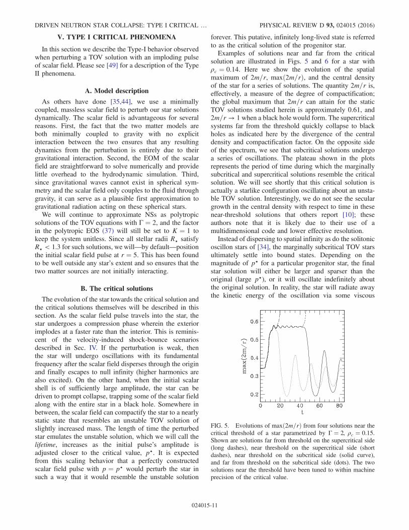
solution are illustrated in Figs. 5 and 6 for a star withρc ¼ 0.14. Here we show the evolution of the spatialmaximum of 2m=r, maxð2m=rÞ, and the central densityof the star for a series of solutions. The quantity 2m=r is,effectively, a measure of the degree of compactification;the global maximum that 2m=r can attain for the staticTOV solutions studied herein is approximately 0.61, and2m=r → 1when a black hole would form. The supercriticalsystems far from the threshold quickly collapse to blackholes as indicated here by the divergence of the centraldensity and compactification factor. On the opposite sideof the spectrum, we see that subcritical solutions undergoa series of oscillations. The plateau shown in the plotsrepresents the period of time during which the marginallysubcritical and supercritical solutions resemble the criticalsolution. We will see shortly that this critical solution isactually a starlike configuration oscillating about an unsta-ble TOV solution. Interestingly, we do not see the seculargrowth in the central density with respect to time in thesenear-threshold solutions that others report [10]; theseauthors note that it is likely due to their use of amultidimensional code and lower effective resolution.Instead of dispersing to spatial infinity as do the solitonic

oscillon stars of [34], the marginally subcritical TOV starsultimately settle into bound states. Depending on themagnitude of p⋆ for a particular progenitor star, the finalstar solution will either be larger and sparser than theoriginal (large p⋆), or it will oscillate indefinitely aboutthe original solution. In reality, the star will radiate awaythe kinetic energy of the oscillation via some viscous

FIG. 5. Evolutions of maxð2m=rÞ from four solutions near thecritical threshold of a star parametrized by Γ ¼ 2, ρc ¼ 0.15.Shown are solutions far from threshold on the supercritical side(long dashes), near threshold on the supercritical side (shortdashes), near threshold on the subcritical side (solid curve),and far from threshold on the subcritical side (dots). The twosolutions near the threshold have been tuned to within machineprecision of the critical value.


024015-11

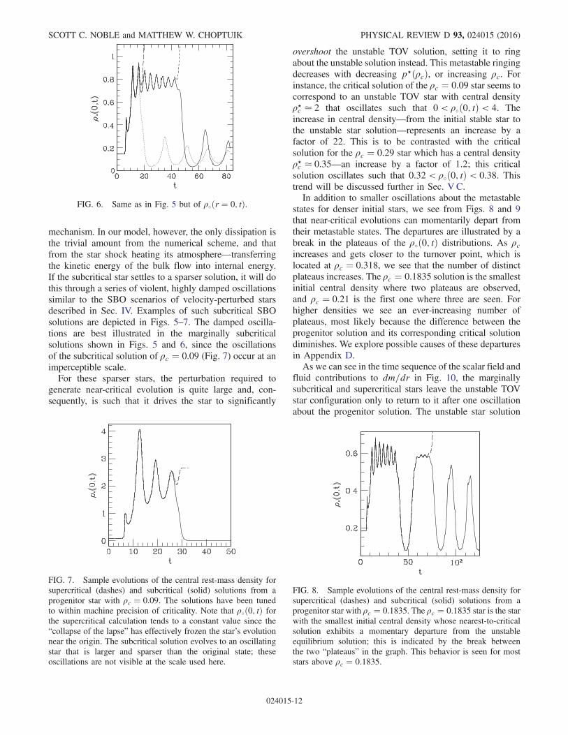
mechanism. In our model, however, the only dissipation isthe trivial amount from the numerical scheme, and thatfrom the star shock heating its atmosphere—transferringthe kinetic energy of the bulk flow into internal energy.If the subcritical star settles to a sparser solution, it will dothis through a series of violent, highly damped oscillationssimilar to the SBO scenarios of velocity-perturbed starsdescribed in Sec. IV. Examples of such subcritical SBOsolutions are depicted in Figs. 5–7. The damped oscilla-tions are best illustrated in the marginally subcriticalsolutions shown in Figs. 5 and 6, since the oscillationsof the subcritical solution of ρc ¼ 0.09 (Fig. 7) occur at animperceptible scale.For these sparser stars, the perturbation required to

generate near-critical evolution is quite large and, con-sequently, is such that it drives the star to significantly

overshoot the unstable TOV solution, setting it to ringabout the unstable solution instead. This metastable ringingdecreases with decreasing p⋆ðρcÞ, or increasing ρc. Forinstance, the critical solution of the ρc ¼ 0.09 star seems tocorrespond to an unstable TOV star with central densityρ⋆c ≃ 2 that oscillates such that 0 < ρ∘ð0; tÞ < 4. Theincrease in central density—from the initial stable star tothe unstable star solution—represents an increase by afactor of 22. This is to be contrasted with the criticalsolution for the ρc ¼ 0.29 star which has a central densityρ⋆c ≃ 0.35—an increase by a factor of 1.2; this criticalsolution oscillates such that 0.32 < ρ∘ð0; tÞ < 0.38. Thistrend will be discussed further in Sec. V C.In addition to smaller oscillations about the metastable

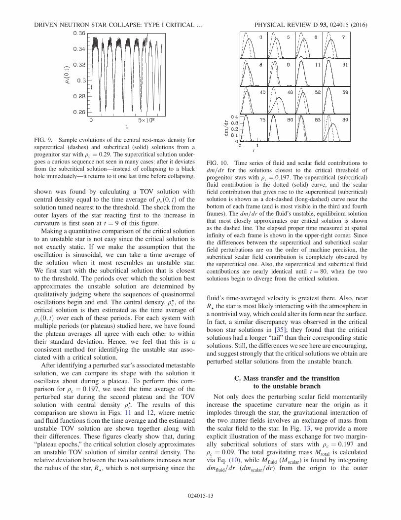
states for denser initial stars, we see from Figs. 8 and 9that near-critical evolutions can momentarily depart fromtheir metastable states. The departures are illustrated by abreak in the plateaus of the ρ∘ð0; tÞ distributions. As ρcincreases and gets closer to the turnover point, which islocated at ρc ¼ 0.318, we see that the number of distinctplateaus increases. The ρc ¼ 0.1835 solution is the smallestinitial central density where two plateaus are observed,and ρc ¼ 0.21 is the first one where three are seen. Forhigher densities we see an ever-increasing number ofplateaus, most likely because the difference between theprogenitor solution and its corresponding critical solutiondiminishes. We explore possible causes of these departuresin Appendix D.As we can see in the time sequence of the scalar field and

fluid contributions to dm=dr in Fig. 10, the marginallysubcritical and supercritical stars leave the unstable TOVstar configuration only to return to it after one oscillationabout the progenitor solution. The unstable star solution

FIG. 6. Same as in Fig. 5 but of ρ∘ðr ¼ 0; tÞ.

FIG. 7. Sample evolutions of the central rest-mass density forsupercritical (dashes) and subcritical (solid) solutions from aprogenitor star with ρc ¼ 0.09. The solutions have been tunedto within machine precision of criticality. Note that ρ∘ð0; tÞ forthe supercritical calculation tends to a constant value since the“collapse of the lapse” has effectively frozen the star’s evolutionnear the origin. The subcritical solution evolves to an oscillatingstar that is larger and sparser than the original state; theseoscillations are not visible at the scale used here.

FIG. 8. Sample evolutions of the central rest-mass density forsupercritical (dashes) and subcritical (solid) solutions from aprogenitor star with ρc ¼ 0.1835. The ρc ¼ 0.1835 star is the starwith the smallest initial central density whose nearest-to-criticalsolution exhibits a momentary departure from the unstableequilibrium solution; this is indicated by the break betweenthe two “plateaus” in the graph. This behavior is seen for moststars above ρc ¼ 0.1835.


024015-12

shown was found by calculating a TOV solution withcentral density equal to the time average of ρ∘ð0; tÞ of thesolution tuned nearest to the threshold. The shock from theouter layers of the star reacting first to the increase incurvature is first seen at t ¼ 9 of this figure.Making a quantitative comparison of the critical solution

to an unstable star is not easy since the critical solution isnot exactly static. If we make the assumption that theoscillation is sinusoidal, we can take a time average ofthe solution when it most resembles an unstable star.We first start with the subcritical solution that is closestto the threshold. The periods over which the solution bestapproximates the unstable solution are determined byqualitatively judging where the sequences of quasinormaloscillations begin and end. The central density, ρ⋆c , of thecritical solution is then estimated as the time average ofρ∘ð0; tÞ over each of these periods. For each system withmultiple periods (or plateaus) studied here, we have foundthe plateau averages all agree with each other to withintheir standard deviation. Hence, we feel that this is aconsistent method for identifying the unstable star asso-ciated with a critical solution.After identifying a perturbed star’s associated metastable

solution, we can compare its shape with the solution itoscillates about during a plateau. To perform this com-parison for ρc ¼ 0.197, we used the time average of theperturbed star during the second plateau and the TOVsolution with central density ρ⋆c. The results of thiscomparison are shown in Figs. 11 and 12, where metricand fluid functions from the time average and the estimatedunstable TOV solution are shown together along withtheir differences. These figures clearly show that, during“plateau epochs,” the critical solution closely approximatesan unstable TOV solution of similar central density. Therelative deviation between the two solutions increases nearthe radius of the star, R⋆, which is not surprising since the

fluid’s time-averaged velocity is greatest there. Also, nearR⋆ the star is most likely interacting with the atmosphere ina nontrivial way, which could alter its form near the surface.In fact, a similar discrepancy was observed in the criticalboson star solutions in [35]; they found that the criticalsolutions had a longer “tail” than their corresponding staticsolutions. Still, the differences we see here are encouraging,and suggest strongly that the critical solutions we obtain areperturbed stellar solutions from the unstable branch.

C. Mass transfer and the transitionto the unstable branch

Not only does the perturbing scalar field momentarilyincrease the spacetime curvature near the origin as itimplodes through the star, the gravitational interaction ofthe two matter fields involves an exchange of mass fromthe scalar field to the star. In Fig. 13, we provide a moreexplicit illustration of the mass exchange for two margin-ally subcritical solutions of stars with ρc ¼ 0.197 andρc ¼ 0.09. The total gravitating mass Mtotal is calculatedvia Eq. (10), while Mfluid (Mscalar) is found by integratingdmfluid=dr (dmscalar=dr) from the origin to the outer

FIG. 10. Time series of fluid and scalar field contributions todm=dr for the solutions closest to the critical threshold ofprogenitor stars with ρc ¼ 0.197. The supercritical (subcritical)fluid contribution is the dotted (solid) curve, and the scalarfield contribution that gives rise to the supercritical (subcritical)solution is shown as a dot-dashed (long-dashed) curve near thebottom of each frame (and is most visible in the third and fourthframes). The dm=dr of the fluid’s unstable, equilibrium solutionthat most closely approximates our critical solution is shownas the dashed line. The elapsed proper time measured at spatialinfinity of each frame is shown in the upper-right corner. Sincethe differences between the supercritical and subcritical scalarfield perturbations are on the order of machine precision, thesubcritical scalar field contribution is completely obscured bythe supercritical one. Also, the supercritical and subcritical fluidcontributions are nearly identical until t ¼ 80, when the twosolutions begin to diverge from the critical solution.

FIG. 9. Sample evolutions of the central rest-mass density forsupercritical (dashes) and subcritical (solid) solutions from aprogenitor star with ρc ¼ 0.29. The supercritical solution under-goes a curious sequence not seen in many cases: after it deviatesfrom the subcritical solution—instead of collapsing to a blackhole immediately—it returns to it one last time before collapsing.


024015-13

boundary. For each case, the nontrivial gravitational inter-action of the fluid and scalar field can be recognized by thesudden change in their integrated masses, which occursnear t ¼ 7 in each plot. The perturbation for the ρc ¼ 0.197star is small and does not transfer a significant portion ofits mass to the star, whereas the perturbation required todrive the ρc ¼ 0.09 star to its marginally subcritical state

transfers more than a third of its mass to the star. Thisdramatic interaction drives the star to oscillate wildly aboutits unstable counterpart—as seen in Fig. 7—and it even-tually expels a great deal of the star’s mass as it departsfrom this highly energetic, yet unstable, bound state. Theloss of the ejected matter from the grid is clearly seen inFig. 13 as the long tail of MfluidðtÞ, which begins todecrease well after the scalar field leaves the grid.To examine how the amount of mass exchange varies for

different critical solutions and to see where exactly criticalsolutions fall on the M⋆ versus ρc graph of equilibriumsolutions, we constructed Fig. 14. The initial star solutionsare indicated here on the left side—the stable branch—while their critical solutions are shown on the right alongthe unstable branch. There are two associated masses foreach critical solution: the mass it would have if its profileexactly matched the unstable TOV solution with the sametime-averaged central density, and its true mass. Both ofthese masses are indicated in Fig. 14 to the right of theturnover point. We find that the total fluid mass is alwayslarger than its initial mass, whereas the mass of the attractorsolution is always smaller than its stable progenitor.In addition, as the turnover is approached, both of thesedeviations diminish until, at turnover, the final mass of thefluid distribution corresponds to its initial mass and themass of the unstable TOV solution.The observed trend that the mass of the unstable TOV

solution is always smaller than the progenitor’s may beexplainable in a number of ways. First, the assumption thatthe oscillations of the critical solution about the attractorsolution are sinusoidal would most likely result in over-estimates of ρc since the oscillations seem to decay in anonlinear fashion over time. A larger ρc would then leadto a mass estimate smaller than it should be, sincedM⋆=dρc < 0 on the unstable branch. Second, it was seen

FIG. 11. Time averages (×’s) of ρ∘ (top) and a (bottom) fromthe marginally subcritical solution compared to those from theassociated unstable TOV solution (ρ⋆∘ and a⋆, dark solid curves) itbest approximates. The subcritical solution used has been tunedto within machine precision of the critical solution, and whoseinitial star has central density of ρc ¼ 0.197. Only every eighthpoint of the time-averaged distributions is displayed. Also shown(light solid curves) are the relative differences between these twosets of functions. The curves are truncated at the stellar radius ofthe critical solution.

FIG. 12. Same as in Fig. 11 but for the functions P (top) andv (bottom).

FIG. 13. Integrated masses of the matter fields as a function oftime for marginally subcritical solutions of progenitor stars withρc ¼ 0.197 (left) and ρc ¼ 0.09 (right). The decrease in Mtotal(solid curve) at the same time as Mscalar (long dashes) vanishessignifies the scalar field leaving the numerical grid; from the timeit leaves, Mtotal is equivalent to Mfluid (short dashes).


024015-14

in Figs. 7–9 that the oscillations of the critical solutionsdecrease with increasing ρc. The decrease in the amount ofenergy in these kinetic modes seems to be correlated withthe decrease in the exchanged mass. A large portion of theexchanged mass must therefore go into the unstable star’skinetic energy.

D. Type I scaling behavior

As the amplitude of the initial pulse of scalar field isadjusted toward p⋆, the lifetime of the metastable, near-critical configuration increases. To quantify the scaling fora given initial star solution, the subcritical solution closestto the critical one is first determined. This is done by tuningthe amplitude of the scalar field pulse, p, until consecutivebisections yield a change in p smaller than machineprecision. Let plo be the value of p that yields thesubcritical solution that most closely approximates thecritical solution. For each p, a unique solution is producedthat resembles this marginally subcritical solution fordifferent lengths of time, determined by how close p isto p⋆. Assuming that the plo solution resembles the criticalsolution longer than any other, the lifetime, T0ðpÞ, is thenthe proper time measured at the origin that elapses untilmax ð2m=rÞ deviates from that of the plo solution by morethan 1%. These lifetimes T0ðpÞ are then fit against theexpected trend (2). An example of such a fit is given inFig. 15. Since supercritical solutions resemble the criticalsolution as well as subcritical solutions, both kinds can beused when determining the scaling exponent σ. The

exponent is the negative of the slope of the fitted line.The deviation of the code-generated data from the best fithas an obvious modulation, which may be due to theperiodic nature of the near-threshold solutions. Similarmodulations in the scaling behavior have also been reportedfor the case of head-on neutron star collisions [11]. Inaddition, we note that the values of σðρ∘Þ are dependent onresolution; from the grid spacing used in the simulationshere and the convergence tests performed with Type IIcritical behavior in [49], we expect the values of σ areaccurate to a few percent. Please see [49] for furtherinformation on tests demonstrating our numerical scheme’svalidity and its second-order rate of convergence in regionsdevoid of shocks.In practice, the lifetime is determined using the proper

time elapsed at spatial infinity, T∞, instead of that measuredat the origin. Let us denote σ∞ as the scaling exponentmeasured with T∞. In order to get the correct scalingexponent, which would correspond to 1=ωLy of theunstable mode, σ∞ must be rescaled. Since T∞ is the sameas our coordinate time, t, then

dT0ðtÞ ¼ αð0; tÞdt: ð42Þ

In order to estimate the rescaling factor, we assume thatαð0; tÞ does not vary much when the solution is in the near-critical regime, so that

αð0; tÞ ≈ α⋆ð0Þ; ð43Þ

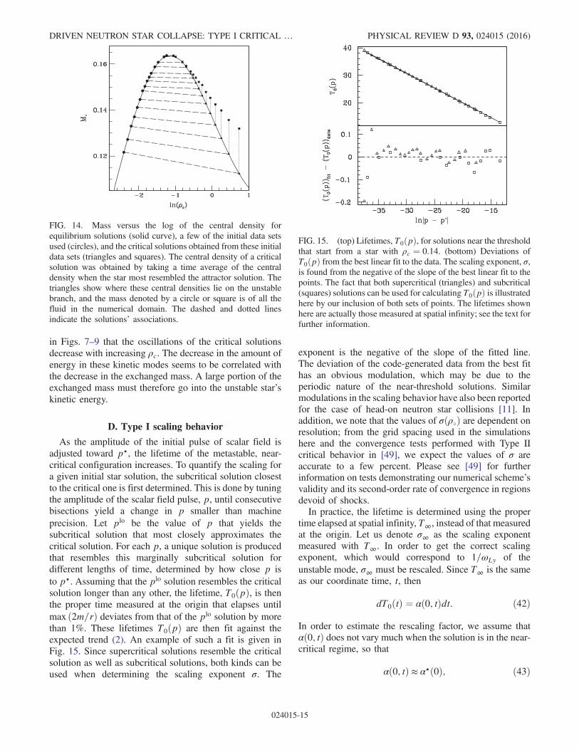
FIG. 15. (top) Lifetimes, T0ðpÞ, for solutions near the thresholdthat start from a star with ρc ¼ 0.14. (bottom) Deviations ofT0ðpÞ from the best linear fit to the data. The scaling exponent, σ,is found from the negative of the slope of the best linear fit to thepoints. The fact that both supercritical (triangles) and subcritical(squares) solutions can be used for calculating T0ðpÞ is illustratedhere by our inclusion of both sets of points. The lifetimes shownhere are actually those measured at spatial infinity; see the text forfurther information.

FIG. 14. Mass versus the log of the central density forequilibrium solutions (solid curve), a few of the initial data setsused (circles), and the critical solutions obtained from these initialdata sets (triangles and squares). The central density of a criticalsolution was obtained by taking a time average of the centraldensity when the star most resembled the attractor solution. Thetriangles show where these central densities lie on the unstablebranch, and the mass denoted by a circle or square is of all thefluid in the numerical domain. The dashed and dotted linesindicate the solutions’ associations.


024015-15

where α⋆ is the central value of the lapse of the unstableTOV solution that corresponds to the critical solution. Thecorrected value of σ is then calculated using

σ ¼ α⋆σ∞: ð44ÞWe have performed fits for σ∞ and then rescaled them

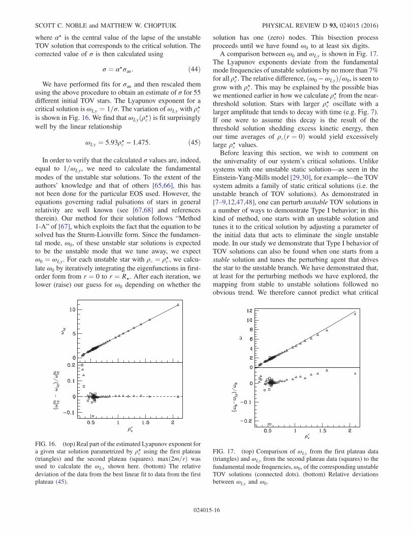
using the above procedure to obtain an estimate of σ for 55different initial TOV stars. The Lyapunov exponent for acritical solution is ωLy ¼ 1=σ. The variation of ωLy with ρ⋆cis shown in Fig. 16. We find that ωLyðρ⋆cÞ is fit surprisinglywell by the linear relationship

ωLy ¼ 5.93ρ⋆c − 1.475: ð45Þ

In order to verify that the calculated σ values are, indeed,equal to 1=ωLy, we need to calculate the fundamentalmodes of the unstable star solutions. To the extent of theauthors’ knowledge and that of others [65,66], this hasnot been done for the particular EOS used. However, theequations governing radial pulsations of stars in generalrelativity are well known (see [67,68] and referencestherein). Our method for their solution follows “Method1-A” of [67], which exploits the fact that the equation to besolved has the Sturm-Liouville form. Since the fundamen-tal mode, ω0, of these unstable star solutions is expectedto be the unstable mode that we tune away, we expectω0 ¼ ωLy. For each unstable star with ρ∘ ¼ ρ⋆c , we calcu-late ω0 by iteratively integrating the eigenfunctions in first-order form from r ¼ 0 to r ¼ R⋆. After each iteration, welower (raise) our guess for ω0 depending on whether the

solution has one (zero) nodes. This bisection processproceeds until we have found ω0 to at least six digits.A comparison between ω0 and ωLy is shown in Fig. 17.

The Lyapunov exponents deviate from the fundamentalmode frequencies of unstable solutions by no more than 7%for all ρ⋆c . The relative difference, ðω0 − ωLyÞ=ω0, is seen togrow with ρ⋆c . This may be explained by the possible biaswe mentioned earlier in how we calculate ρ⋆c from the near-threshold solution. Stars with larger ρ⋆c oscillate with alarger amplitude that tends to decay with time (e.g. Fig. 7).If one were to assume this decay is the result of thethreshold solution shedding excess kinetic energy, thenour time averages of ρ∘ðr ¼ 0Þ would yield excessivelylarge ρ⋆c values.Before leaving this section, we wish to comment on

the universality of our system’s critical solutions. Unlikesystems with one unstable static solution—as seen in theEinstein-Yang-Mills model [29,30], for example—the TOVsystem admits a family of static critical solutions (i.e. theunstable branch of TOV solutions). As demonstrated in[7–9,12,47,48], one can perturb unstable TOV solutions ina number of ways to demonstrate Type I behavior; in thiskind of method, one starts with an unstable solution andtunes it to the critical solution by adjusting a parameter ofthe initial data that acts to eliminate the single unstablemode. In our study we demonstrate that Type I behavior ofTOV solutions can also be found when one starts from astable solution and tunes the perturbing agent that drivesthe star to the unstable branch. We have demonstrated that,at least for the perturbing methods we have explored, themapping from stable to unstable solutions followed noobvious trend. We therefore cannot predict what critical

FIG. 16. (top) Real part of the estimated Lyapunov exponent fora given star solution parametrized by ρ⋆c using the first plateau(triangles) and the second plateau (squares). maxð2m=rÞ wasused to calculate the ωLy shown here. (bottom) The relativedeviation of the data from the best linear fit to data from the firstplateau (45).

FIG. 17. (top) Comparison of ωLy from the first plateau data(triangles) and ωLy from the second plateau data (squares) to thefundamental mode frequencies, ω0, of the corresponding unstableTOV solutions (connected dots). (bottom) Relative deviationsbetween ωLy and ω0.


024015-16

solution a particular set of initial data will tend toward. Onthe other hand, the calculations performed by the othersbegin with initial data very near an unstable solution thatis ultimately identified with a critical solution. Thesecomputations demonstrate that the unstable branch servesas a family of 1-mode unstable solutions, whereas ourmethod additionally demonstrates that the unstable branchis the family of 1-mode unstable solutions to which stablesolutions are attracted—at least for the scenarios weexamined.

VI. CONCLUSION

In this paper, we simulated spherically symmetricrelativistic perfect fluid flow in the strong-field regimeof general relativity. Specifically, a perfect fluid that admitsa length scale, for example one that follows a relativisticideal gas law, was used to investigate the dynamics ofcompact, stellar objects. A stiff equation of state was usedto approximate the behavior of some realistic state equa-tions for NS matter. The stars served as initial data for aparameter survey, in which we drove them to collapse usingeither an initial velocity profile or a pulse of massless scalarfield. Both types of critical phenomena were observedusing each of the two mechanisms. The parameter spacesurvey provided a description of the boundary betweenType I and Type II behavior, and illustrated the wide rangeof dynamical scenarios involved in stellar collapse. Wefound that the non–black hole end states of solutions nearthe threshold of black hole seemed to be correlated to thetype of critical behavior observed. For instance, Type Ibehavior seemed to always entail subcritical end states thatwere bound and starlike. Type II behavior, on the otherhand, was observed to coincide with dispersal end states.Since the unstable branch of TOV solutions has been

known for decades, many anticipated that TOV solutionswould exhibit some kind of Type I behavior. This paperdescribes the first in depth analysis of Type I phenomenaassociated with hydrostatic solutions in that the Lyapunovexponents of the critical solutions were measured for avariety of cases. We verified that the Lyapunov exponentsagree well with the normal mode frequency of theirassociated unstable TOV solutions, confirming that thecritical solutions are TOV solutions on the unstable branch.The exponents were found to follow a linear relationship asa function of the time-averaged central densities of theirassociated critical solutions. We also discovered that theType I critical solutions coincided with perturbed unstablehydrostatic solutions which were typically more massivethan their progenitor stars.In the future, we hope to address a great number of topics

that expand on this work. First, the supercritical section ofparameter space demands further exploration in order toinvestigate how much matter can realistically be ejectedfrom shock/bounce/collapse scenarios. In addition, theability to follow spacetimes after the formation of an

apparent horizon would allow us to study the possiblesimultaneous overlap of Type I and Type II behavior. Itwould also allow us to measure the ultimate mass distri-bution of black holes, as we are able only to measure theblack hole masses at the time of formation which neglectsany subsequent mass accretion. Ultimately, it is our goal toexpand the model a great deal, making the matter descrip-tion more realistic and eliminating symmetry. As a firststep, we wish to develop adaptive mesh refinement proce-dures for conservative systems that will be required to studycritical phenomena of stellar objects in axial symmetry[69]. Also, we wish to examine how Type II behaviorchanges in the context of realistic equations of state. Forexample, realistic equations of state effectively make theadiabatic index of the fluid a function of the fluid’s densityand temperature, and, to date, critical behavior in perfectfluids has only been described for fluids with constantadiabatic index.

ACKNOWLEDGMENTS

The authors wish to acknowledge financial support fromCIFAR, NSERC, NSF PHY 02-05155, and NSF CDI AST10-28087. S. C. N. wishes to thank I. Olabarrieta for manyhelpful comments. All numerical calculations were per-formed on UBC’s vn PIII and vnp4 clusters (supported byCFI and BCKDF).

APPENDIX A: CONVERSIONOF UNITS AND SCALE

When theoretical calculations are made in the theory ofgeneral relativity, it is customary to use “geometrized units”in which G ¼ c ¼ 1 (see Appendix E of [50] for acomprehensive discussion on the conversion to and fromgeometrized units, only a few key ideas will be mentionedhere). In such units, scales or dimensions of mass (M) andtime (T) are transformed into scales of length (L) only, bymultiplying by appropriate factors ofG and c. For instance,because of how G and c scale with mass and time, one caneasily derive that a quantity Q that scales like LlMmTt canbe converted into geometrized units by multiplication ofctðG=c2Þm. After the conversion to geometrized units, Qscales as Llþmþt.Since the equations governing the ultrarelativistic

fluid are all invariant under changes in the fundamentallength scale L, such fluids naturally follow self-similarbehavior [70]. The inclusion of ρ∘ in the system elimi-nates this intrinsic scale invariance via the EOS. Forexample, when using the polytropic EOS, P ¼ KρΓ∘ , theconstantK has dimensions L2ðΓ−1Þ in geometrized units andL3Γ−1M1−ΓT−2 in nongeometrized units. Hence, one mayset the fundamental length scale of the system by choosinga value for K [58,71]. Since all physical quantities areexpressible in dimensions of L in geometrized units, thequantities of static and dynamic systems which use one set


024015-17

fK;Γg should be exactly the same as those using anotherset fK̂; Γ̂g, modulo a rescaling of each quantity by thefactor

ðL̂=LÞn ¼ ðK̂1=2ðΓ̂−1Þ=K1=2ðΓ−1ÞÞn; ðA1Þwhere n depends on how the particular quantity scales withlength. Thus, setting K ¼ 1 makes the system dimension-less, and this is the approach used in the paper. This choicesimplifies the comparison of two solutions having differentvalues of K and Γ.In order to transform from our dimensionless system to

one with dimensions, one must first set the scale by fixingK. Let X̂ be a quantity that has dimensions of LlMmTt, andX be the corresponding dimensionless quantity. In order totransform X into X̂, one may use the following equation:

X̂ ¼ KxcyGzX; ðA2Þwhere

x ¼ lþmþ t2ðΓ − 1Þ ; z ¼ −

lþ 3mþ t2

ðA3Þ

y ¼ ðΓ − 2Þlþ ð3Γ − 4Þm − tΓ − 1

: ðA4Þ

When presenting results of TOV solutions using poly-tropic state equations, it is customary to choose K in such away that the maximum stable mass for the given polytropecorresponds to that of the Chandrasekhar mass, 1.4M⊙.As an example, a mass M̂ðKÞ expressed in units can becalculated from the dimensionless MðK ¼ 1Þ via theabove formula (since M̂ has dimensions of only mass,then l ¼ 0, m ¼ 1, t ¼ 0):

M̂ðKÞ ¼ K1=2ðΓ−1Þc3c−1=ðΓ−1ÞG−3=2MðK ¼ 1Þ: ðA5Þ

Since the TOV solutions for Γ ¼ 2 and K ¼ 1 yield amaximum stable mass of 0.164, then the K thatwould make M̂ðKÞ ¼ 1.4M⊙ would be approximately105 cm5 g−1 s−2, in cgs units. The radius of this maximummass star is 0.768 with K ¼ 1, and is about 9.4 kmwith K ¼ 105 cm5 g−1 s−2.

APPENDIX B: CALCULATING THE INITIALSTAR SOLUTION WITH AN INGOING

COORDINATE VELOCITY

Initializing the star with a certain coordinate velocityinstead of the Eulerian velocity, v ¼ aU=α, couples theHamiltonian constraint (4) and the slicing condition (7) byintroducing α and a into their right-hand sides. In order toexplicitly show how the right-hand sides change, the con-served variables must be expressed in terms of the coordinatevelocity and primitive variables via Eqs. (26)–(28):

a0

a¼ a2

�4πr

�ρ∘h

1 − ðaUα Þ2− P

�−

1

2r2

�þ 1

2r2; ðB1Þ

α0

α¼ a2

�4πr

�ρ∘h

ðaU=αÞ21 − ðaUα Þ2

þ P

�þ 1

2r2

�−

1

2r2: ðB2Þ

The coupling of these equations complicates theirnumerical solution. We will briefly describe how theyare solved here. We start by solving the TOV equations,adjusting the lapse so that αajr¼rmax

¼ 1. Given U∘, UðrÞ isspecified via Eq. (41), and α; a are recalculated via a two-dimensional Newton-Raphson method which solvesEqs. (B1) and (B2) at each grid point. The integrationstarts at the origin with αðr ¼ 0Þ, aðr ¼ 0Þ from the TOVsolution. The Eulerian velocity, v ¼ Ua=α, is calculatedusing α; a at this stage. Since the parametrization for α ischosen at the origin, the outer boundary condition,αajr¼rmax

¼ 1, will not necessarily be satisfied. In orderto impose this outer boundary condition and calculate thefinal values of αðrÞ and aðrÞ, the uncoupled Hamiltonianconstraint (4) and slicing condition (7) are then solvedusing the v calculated in the previous step.

APPENDIX C: PERTURBED NEUTRON STAREND STATES

Differentiating between some of the types of outcomes isdifficult. To aid in this process, we examined how variousquantities varied with time at the star’s radius, R⋆ðtÞ. Wedefine R⋆ð0Þ as the radius of the last numerical cell beforewhich ρ∘ falls below the floor density [72], and set R⋆ðtÞto be the radius at which ρ∘ðr; tÞ ¼ ρ∘ðR⋆ð0Þ; 0Þ to withinsome finite precision. This served as a fair approximationto the worldline of the fluid element originally at R⋆ð0Þ,however, we do not assume that R⋆ðtÞ is that of aLagrangian observer. The Eulerian velocity at r ¼ R⋆ðtÞis also considered and will be referred to as v⋆.The boundary between SBO and O outcomes may be the

most imprecisely determined one. This is due to the factthat the shock in SBO cases weakens as the perturbation isreduced, making it difficult to tell if a bounce actuallyhappens and whether the subsequent oscillations take placeabout a different star solution. In addition, an O systemmay form a minor shock at first, but still maintain nearlyconstant amplitude oscillations, indicating the absence ofsignificant shock heating. Herein, an O state is defined as astar which lost less than 1% of its mass over the first sixperiods of its fundamental mode of oscillation. This choiceof cutoff is motivated by two facts: (1) evolutions whichseem to be oscillating about the initial solution still losemass, because the oscillations still eject minute amounts ofmatter from the star’s surface; (2) those evolutions whichare obviously SBO seem to eject most of the expelledmatter within the first 6 oscillations. Using this definition,


024015-18

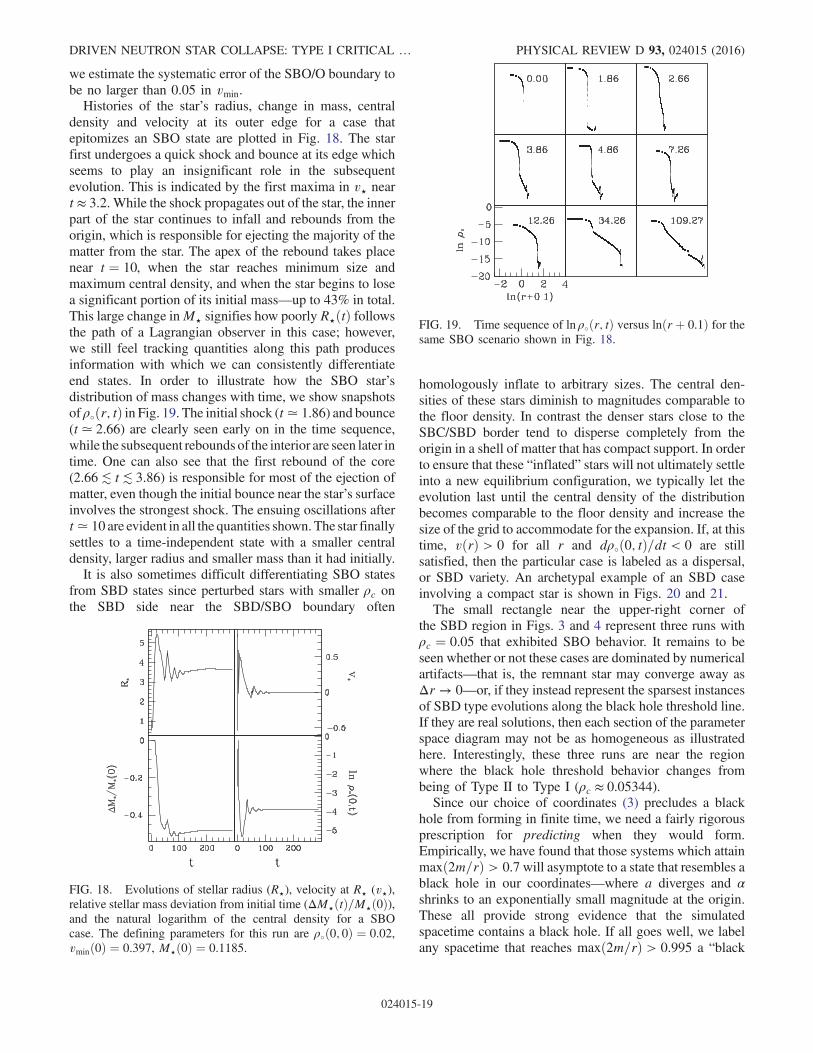
we estimate the systematic error of the SBO/O boundary tobe no larger than 0.05 in vmin.Histories of the star’s radius, change in mass, central

density and velocity at its outer edge for a case thatepitomizes an SBO state are plotted in Fig. 18. The starfirst undergoes a quick shock and bounce at its edge whichseems to play an insignificant role in the subsequentevolution. This is indicated by the first maxima in v⋆ neart ≈ 3.2. While the shock propagates out of the star, the innerpart of the star continues to infall and rebounds from theorigin, which is responsible for ejecting the majority of thematter from the star. The apex of the rebound takes placenear t ¼ 10, when the star reaches minimum size andmaximum central density, and when the star begins to losea significant portion of its initial mass—up to 43% in total.This large change inM⋆ signifies how poorly R⋆ðtÞ followsthe path of a Lagrangian observer in this case; however,we still feel tracking quantities along this path producesinformation with which we can consistently differentiateend states. In order to illustrate how the SBO star’sdistribution of mass changes with time, we show snapshotsof ρ∘ðr; tÞ in Fig. 19. The initial shock (t≃ 1.86) and bounce(t≃ 2.66) are clearly seen early on in the time sequence,while the subsequent rebounds of the interior are seen later intime. One can also see that the first rebound of the core(2.66≲ t≲ 3.86) is responsible for most of the ejection ofmatter, even though the initial bounce near the star’s surfaceinvolves the strongest shock. The ensuing oscillations aftert≃ 10 are evident in all the quantities shown. The star finallysettles to a time-independent state with a smaller centraldensity, larger radius and smaller mass than it had initially.It is also sometimes difficult differentiating SBO states

from SBD states since perturbed stars with smaller ρc onthe SBD side near the SBD/SBO boundary often

homologously inflate to arbitrary sizes. The central den-sities of these stars diminish to magnitudes comparable tothe floor density. In contrast the denser stars close to theSBC/SBD border tend to disperse completely from theorigin in a shell of matter that has compact support. In orderto ensure that these “inflated” stars will not ultimately settleinto a new equilibrium configuration, we typically let theevolution last until the central density of the distributionbecomes comparable to the floor density and increase thesize of the grid to accommodate for the expansion. If, at thistime, vðrÞ > 0 for all r and dρ∘ð0; tÞ=dt < 0 are stillsatisfied, then the particular case is labeled as a dispersal,or SBD variety. An archetypal example of an SBD caseinvolving a compact star is shown in Figs. 20 and 21.The small rectangle near the upper-right corner of

the SBD region in Figs. 3 and 4 represent three runs withρc ¼ 0.05 that exhibited SBO behavior. It remains to beseen whether or not these cases are dominated by numericalartifacts—that is, the remnant star may converge away asΔr → 0—or, if they instead represent the sparsest instancesof SBD type evolutions along the black hole threshold line.If they are real solutions, then each section of the parameterspace diagram may not be as homogeneous as illustratedhere. Interestingly, these three runs are near the regionwhere the black hole threshold behavior changes frombeing of Type II to Type I (ρc ≈ 0.05344).Since our choice of coordinates (3) precludes a black

hole from forming in finite time, we need a fairly rigorousprescription for predicting when they would form.Empirically, we have found that those systems which attainmaxð2m=rÞ > 0.7will asymptote to a state that resembles ablack hole in our coordinates—where a diverges and αshrinks to an exponentially small magnitude at the origin.These all provide strong evidence that the simulatedspacetime contains a black hole. If all goes well, we labelany spacetime that reaches maxð2m=rÞ > 0.995 a “black

FIG. 18. Evolutions of stellar radius (R⋆), velocity at R⋆ (v⋆),relative stellar mass deviation from initial time (ΔM⋆ðtÞ=M⋆ð0Þ),and the natural logarithm of the central density for a SBOcase. The defining parameters for this run are ρ∘ð0; 0Þ ¼ 0.02,vminð0Þ ¼ 0.397, M⋆ð0Þ ¼ 0.1185.

FIG. 19. Time sequence of ln ρ∘ðr; tÞ versus lnðrþ 0.1Þ for thesame SBO scenario shown in Fig. 18.


024015-19

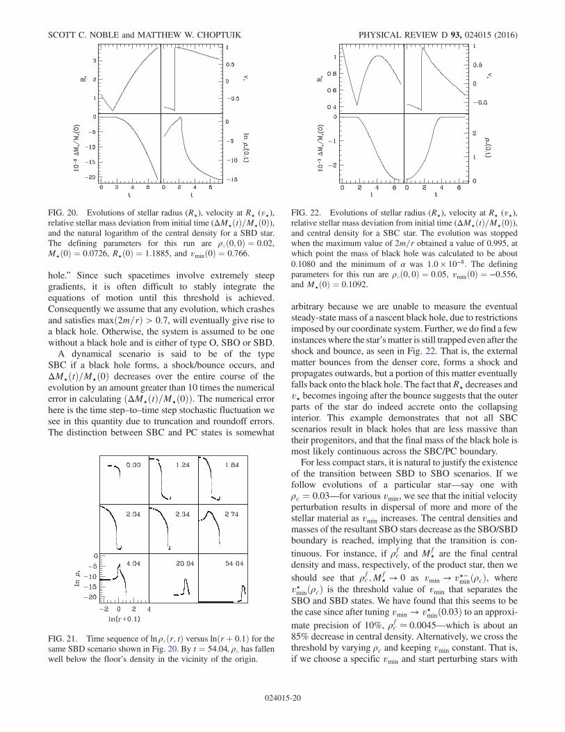
hole.” Since such spacetimes involve extremely steepgradients, it is often difficult to stably integrate theequations of motion until this threshold is achieved.Consequently we assume that any evolution, which crashesand satisfies maxð2m=rÞ > 0.7, will eventually give rise toa black hole. Otherwise, the system is assumed to be onewithout a black hole and is either of type O, SBO or SBD.A dynamical scenario is said to be of the type

SBC if a black hole forms, a shock/bounce occurs, andΔM⋆ðtÞ=M⋆ð0Þ decreases over the entire course of theevolution by an amount greater than 10 times the numericalerror in calculating ðΔM⋆ðtÞ=M⋆ð0ÞÞ. The numerical errorhere is the time step–to–time step stochastic fluctuation wesee in this quantity due to truncation and roundoff errors.The distinction between SBC and PC states is somewhat

arbitrary because we are unable to measure the eventualsteady-state mass of a nascent black hole, due to restrictionsimposed by our coordinate system. Further, we do find a fewinstanceswhere the star’smatter is still trapped even after theshock and bounce, as seen in Fig. 22. That is, the externalmatter bounces from the denser core, forms a shock andpropagates outwards, but a portion of this matter eventuallyfalls back onto the black hole. The fact thatR⋆ decreases andv⋆ becomes ingoing after the bounce suggests that the outerparts of the star do indeed accrete onto the collapsinginterior. This example demonstrates that not all SBCscenarios result in black holes that are less massive thantheir progenitors, and that the final mass of the black hole ismost likely continuous across the SBC/PC boundary.For less compact stars, it is natural to justify the existence

of the transition between SBD to SBO scenarios. If wefollow evolutions of a particular star—say one withρc ¼ 0.03—for various vmin, we see that the initial velocityperturbation results in dispersal of more and more of thestellar material as vmin increases. The central densities andmasses of the resultant SBO stars decrease as the SBO/SBDboundary is reached, implying that the transition is con-tinuous. For instance, if ρfc and Mf⋆ are the final centraldensity and mass, respectively, of the product star, then weshould see that ρfc;M

f⋆ → 0 as vmin → v⋆−minðρcÞ, wherev⋆minðρcÞ is the threshold value of vmin that separates theSBO and SBD states. We have found that this seems to bethe case since after tuning vmin → v⋆minð0.03Þ to an approxi-mate precision of 10%, ρfc ≃ 0.0045—which is about an85% decrease in central density. Alternatively, we cross thethreshold by varying ρc and keeping vmin constant. That is,if we choose a specific vmin and start perturbing stars with

FIG. 20. Evolutions of stellar radius (R⋆), velocity at R⋆ (v⋆),relative stellar mass deviation from initial time (ΔM⋆ðtÞ=M⋆ð0Þ),and the natural logarithm of the central density for a SBD star.The defining parameters for this run are ρ∘ð0; 0Þ ¼ 0.02,M⋆ð0Þ ¼ 0.0726, R⋆ð0Þ ¼ 1.1885, and vminð0Þ ¼ 0.766.

FIG. 21. Time sequence of ln ρ∘ðr; tÞ versus lnðrþ 0.1Þ for thesame SBD scenario shown in Fig. 20. By t ¼ 54.04, ρ∘ has fallenwell below the floor’s density in the vicinity of the origin.

FIG. 22. Evolutions of stellar radius (R⋆), velocity at R⋆ (v⋆),relative stellar mass deviation from initial time (ΔM⋆ðtÞ=M⋆ð0Þ),and central density for a SBC star. The evolution was stoppedwhen the maximum value of 2m=r obtained a value of 0.995, atwhich point the mass of black hole was calculated to be about0.1080 and the minimum of α was 1.0 × 10−8. The definingparameters for this run are ρ∘ð0; 0Þ ¼ 0.05, vminð0Þ ¼ −0.556,and M⋆ð0Þ ¼ 0.1092.


024015-20

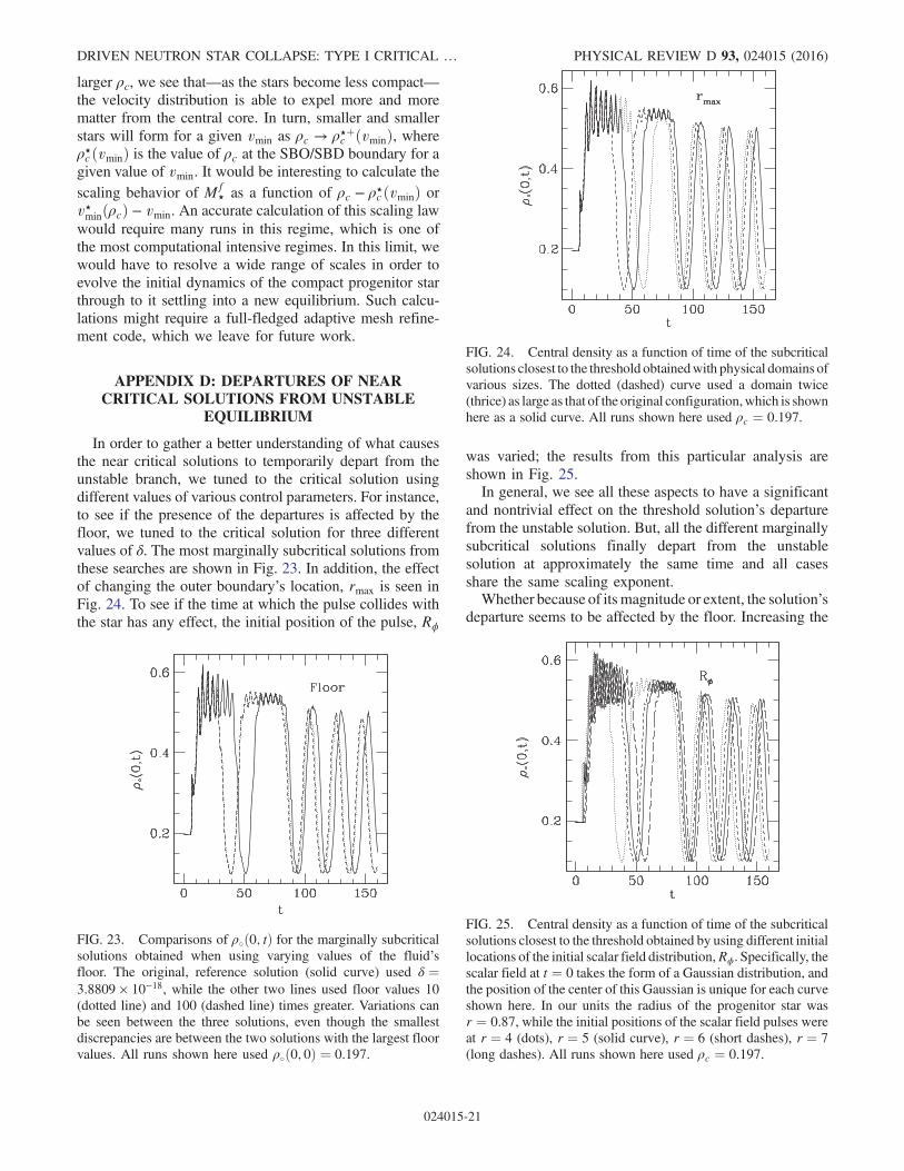
larger ρc, we see that—as the stars become less compact—the velocity distribution is able to expel more and morematter from the central core. In turn, smaller and smallerstars will form for a given vmin as ρc → ρ⋆þc ðvminÞ, whereρ⋆cðvminÞ is the value of ρc at the SBO/SBD boundary for agiven value of vmin. It would be interesting to calculate thescaling behavior of Mf⋆ as a function of ρc − ρ⋆c ðvminÞ orv⋆minðρcÞ − vmin. An accurate calculation of this scaling lawwould require many runs in this regime, which is one ofthe most computational intensive regimes. In this limit, wewould have to resolve a wide range of scales in order toevolve the initial dynamics of the compact progenitor starthrough to it settling into a new equilibrium. Such calcu-lations might require a full-fledged adaptive mesh refine-ment code, which we leave for future work.

APPENDIX D: DEPARTURES OF NEARCRITICAL SOLUTIONS FROM UNSTABLE

EQUILIBRIUM

In order to gather a better understanding of what causesthe near critical solutions to temporarily depart from theunstable branch, we tuned to the critical solution usingdifferent values of various control parameters. For instance,to see if the presence of the departures is affected by thefloor, we tuned to the critical solution for three differentvalues of δ. The most marginally subcritical solutions fromthese searches are shown in Fig. 23. In addition, the effectof changing the outer boundary’s location, rmax is seen inFig. 24. To see if the time at which the pulse collides withthe star has any effect, the initial position of the pulse, Rϕ

was varied; the results from this particular analysis areshown in Fig. 25.In general, we see all these aspects to have a significant

and nontrivial effect on the threshold solution’s departurefrom the unstable solution. But, all the different marginallysubcritical solutions finally depart from the unstablesolution at approximately the same time and all casesshare the same scaling exponent.Whether because of its magnitude or extent, the solution’s

departure seems to be affected by the floor. Increasing the

FIG. 24. Central density as a function of time of the subcriticalsolutions closest to the threshold obtainedwith physical domains ofvarious sizes. The dotted (dashed) curve used a domain twice(thrice) as large as that of the original configuration,which is shownhere as a solid curve. All runs shown here used ρc ¼ 0.197.

FIG. 23. Comparisons of ρ∘ð0; tÞ for the marginally subcriticalsolutions obtained when using varying values of the fluid’sfloor. The original, reference solution (solid curve) used δ ¼3.8809 × 10−18, while the other two lines used floor values 10(dotted line) and 100 (dashed line) times greater. Variations canbe seen between the three solutions, even though the smallestdiscrepancies are between the two solutions with the largest floorvalues. All runs shown here used ρ∘ð0; 0Þ ¼ 0.197.

FIG. 25. Central density as a function of time of the subcriticalsolutions closest to the threshold obtained by using different initiallocations of the initial scalar field distribution,Rϕ. Specifically, thescalar field at t ¼ 0 takes the form of a Gaussian distribution, andthe position of the center of this Gaussian is unique for each curveshown here. In our units the radius of the progenitor star wasr ¼ 0.87, while the initial positions of the scalar field pulses wereat r ¼ 4 (dots), r ¼ 5 (solid curve), r ¼ 6 (short dashes), r ¼ 7(long dashes). All runs shown here used ρc ¼ 0.197.


024015-21

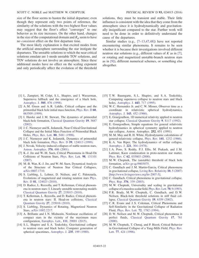
size of the floor seems to hasten the initial departure; eventhough they represent only two points of reference, thesimilarity of the solutions with the two highest floor valuesmay suggest that the floor’s effect “converges” to onebehavior as its size increases. On the other hand, changesin the size of the computational domain andRϕ seem to haveno consistent effect on the first departure time.The most likely explanation is that excited modes from

the artificial atmosphere surrounding the star instigate thedepartures. The unstable solutions to which the near criticalsolutions emulate are 1-mode unstable TOV solutions, andTOV solutions do not involve an atmosphere. Since theseadditional modes have no effect on the scaling exponentand only periodically affect the evolution of the threshold

solutions, they must be transient and stable. Their littleinfluence is consistent with the idea that they come from theatmosphere since it is hydrodynamically and gravitation-ally insignificant compared to the star. Further work willneed to be done in order to definitively understand thecause of the departures.Similar studies (e.g., [7–13,47,48]) have not reported

encountering similar phenomena. It remains to be seenwhether it is because their investigations involved differentneutron star solutions (e.g., different values of K as in [7],or rotating and magnetized unstable-branch neutron starsas in [9]), different numerical schemes, or something elsealtogether.

[1] L. Zampieri, M. Colpi, S. L. Shapiro, and I. Wasserman,Supernova fallback and the emergence of a black hole,Astrophys. J. 505, 876 (1998).

[2] A. M. Green and A. R. Liddle, Critical collapse and theprimordial black hole initial mass function, Phys. Rev. D 60,063509 (1999).

[3] I. Hawke and J. M. Stewart, The dynamics of primordialblack-hole formation, Classical Quantum Gravity 19, 3687(2002).

[4] J. C. Niemeyer and K. Jedamzik, Near-Critical GravitationalCollapse and the Initial Mass Function of Primordial BlackHoles, Phys. Rev. Lett. 80, 5481 (1998).

[5] J. C. Niemeyer and K. Jedamzik, Dynamics of primordialblack hole formation, Phys. Rev. D 59, 124013 (1999).

[6] J. Novak, Velocity-induced collapses of stable neutron stars,Astron. Astrophys. 376, 606 (2001).

[7] K.-J. Jin and W.-M. Suen, Critical Phenomena in Head-OnCollisions of Neutron Stars, Phys. Rev. Lett. 98, 131101(2007).

[8] M.-B. Wan, K.-J. Jin, and W.-M. Suen, Dynamical Analysisof the Structure of Neutron Star Critical Collapses,arXiv:0807.1710.

[9] S. Liebling, L. Lehner, D. Neilsen, and C. Palenzuela,Evolutions of magnetized and rotating neutron stars Phys.Rev. D 81, 124023 (2010).

[10] D. Radice, L. Rezzolla, and T. Kellerman, Critical phenom-ena in neutron stars: I. Linearly unstable nonrotating modelsClassical Quantum Gravity 27, 235015 (2010).

[11] T. Kellerman, L. Rezzolla, and D. Radice, Critical phenom-ena in neutron stars: II. Head-on collisions, ClassicalQuantum Gravity 27, 235016 (2010).

[12] S. Liebling, Dynamics of Rotating, Magnetized NeutronStars, arXiv:1002.2217.

[13] A. Brillante and I. N. Mishustin, Nonlinear oscillations ofcompact stars in the vicinity of the maximum massconfiguration, Europhys. Lett., 111, 29001 (2015).

[14] S. L. Shapiro and S. A. Teukolsky, Gravitational collapseto neutron stars and black holes: Computer generation ofspherical spacetimes, Astrophys. J. 235, 199 (1980).

[15] T. W. Baumgarte, S. L. Shapiro, and S. A. Teukolsky,Computing supernova collapse to neutron stars and blackholes, Astrophys. J. 443, 717 (1995).

[16] W. C. Hernandez Jr. and C.W. Misner, Observer time as acoordinate in relativistic spherical hydrodynamics,Astrophys. J. 143, 452 (1966).

[17] E. Gourgoulhon, 1D numerical relativity applied to neutronstar collapse, Classical Quantum Gravity 9, S117 (1992).

[18] E. Gourgoulhon, Simple equations for general relativistichydrodynamics in spherical symmetry applied to neutronstar collapse, Astron. Astrophys. 252, 651 (1991).

[19] M.M. May and R. H. White, Hydrodynamic calculations ofgeneral-relativistic collapse, Phys. Rev. 141, 1232 (1966).

[20] K. A. Van Riper, The hydrodynamics of stellar collapse,Astrophys. J. 221, 304 (1978).

[21] J. A. Pons, S. Reddy, P. J. Ellis, M. Prakash, and J. M.Lattimer, Kaon condensation in proto-neutron star matter,Phys. Rev. C 62, 035803 (2000).

[22] M.W. Choptuik, The (unstable) threshold of black holeformation, arXiv:gr-qc/9803075.

[23] C. Gundlach and J. M. Martin-Garcia, Critical phenomenain gravitational collapse, Living Rev. Relativity 10, 5 (2007)[http://www.livingreviews.org/lrr‑2007‑5].

[24] C. Gundlach, Critical phenomena in gravitational collapse,Phys. Rep. 376, 339 (2003).

[25] M.W. Choptuik, Universality and scaling in gravitationalcollapseof amassless scalar field, Phys.Rev.Lett.70, 9 (1993).

[26] P. R. Brady, M.W. Choptuik, C. Gundlach, and D.W.Neilsen, Black-hole threshold solutions in stiff fluid col-lapse, Classical Quantum Gravity 19, 6359 (2002).

[27] C. R. Evans and J. S. Coleman, Critical Phenomena andSelf-Similarity in the Gravitational Collapse of RadiationFluid, Phys. Rev. Lett. 72, 1782 (1994).

[28] D.W. Neilsen and M.W. Choptuik, Critical phenomena inperfect fluids, Classical Quantum Gravity 17, 761(2000).

[29] M.W. Choptuik, T. Chmaj, and P. Bizoń, Critical Behaviorin Gravitational Collapse of a Yang-Mills Field, Phys. Rev.Lett. 77, 424 (1996).


024015-22

http://dx.doi.org/10.1086/306192



http://dx.doi.org/10.1088/0264-9381/19/14/310

http://dx.doi.org/10.1088/0264-9381/19/14/310

http://dx.doi.org/10.1103/PhysRevLett.80.5481


http://dx.doi.org/10.1051/0004-6361:20011037



http://arXiv.org/abs/0807.1710



http://dx.doi.org/10.1088/0264-9381/27/23/235015

http://dx.doi.org/10.1088/0264-9381/27/23/235016

http://dx.doi.org/10.1088/0264-9381/27/23/235016


http://dx.doi.org/10.1209/0295-5075/111/29001

http://dx.doi.org/10.1086/157625

http://dx.doi.org/10.1086/175563

http://dx.doi.org/10.1086/148525

http://dx.doi.org/10.1088/0264-9381/9/S/005

http://dx.doi.org/10.1103/PhysRev.141.1232

http://dx.doi.org/10.1086/156029

http://dx.doi.org/10.1103/PhysRevC.62.035803

http://arXiv.org/abs/gr-qc/9803075

http://dx.doi.org/10.12942/lrr-2007-5

http://www.livingreviews.org/lrr-2007-5



http://dx.doi.org/10.1016/S0370-1573(02)00560-4


http://dx.doi.org/10.1088/0264-9381/19/24/306


http://dx.doi.org/10.1088/0264-9381/17/4/303

http://dx.doi.org/10.1088/0264-9381/17/4/303



[30] M.W. Choptuik, E. W. Hirschmann, and R. L. Marsa, Newcritical behavior in Einstein-Yang-Mills collapse, Phys. Rev.D 60, 124011 (1999).

[31] I. Olabarrieta and M.W. Choptuik, Critical phenmena at thethreshold of black hole formation for collisionless matter inspherical symmetry, Phys. Rev. D 65, 024007 (2001).

[32] G. Rein, A. D. Rendall, and J. Schaeffer, Critical collapse ofcollisionless matter: A numerical investigation, Phys. Rev.D 58, 044007 (1998).

[33] T. Koike, T. Hara, and S. Adachi, Critical Behavior inGravitational Collapse of Radiation Fluid: A Renormaliza-tion Group (Linear Perturbation) Analysis, Phys. Rev. Lett.74, 5170 (1995).

[34] P. R. Brady, C. M. Chambers, and S. M. C. V. Gonçalves,Phases of massive scalar field collapse, Phys. Rev. D 56,R6057 (1997).

[35] S. H. Hawley and M.W. Choptuik, Boson stars driven tothe brink of black hole formation, Phys. Rev. D 62, 104024(2000).

[36] C. W. Lai and M.W. Choptuik, Final fate of subcriticalevolutions of boson stars, arXiv:0709.0324v1.

[37] J. R. Oppenheimer and G. M. Volkoff, On massive neutroncores, Phys. Rev. 55, 374 (1939).

[38] R. C. Tolman, Relativity, Thermodynamics and Cosmology(Oxford University Press, New York, 1934).

[39] R. C. Tolman, Static solutions of Einstein’s field equationsfor spheres of fluid, Phys. Rev. 55, 364 (1939).

[40] P. Jetzer, Boson stars, Phys. Rep. 220, 163 (1992).[41] T. D. Lee and Y. Pang, Nontopological solitons, Phys. Rep.

221, 251 (1992).[42] S. C. Noble, A numerical study of relativistic fluid collapse,

arXiv:gr-qc/0310116.[43] S. H. Hawley (private communication).[44] F. Siebel, J. A. Font, and P. Papadopoulos, Scalar field

induced oscillations of relativistic stars and gravitationalcollapse, Phys. Rev. D 65, 024021 (2001).

[45] J. A. Font, T. Goodale, S. Iyer, M. Miller, L. Rezzolla, E.Seidel, N. Stergioulas, W. Suen, and M. Tobias, Three-dimensional numerical general relativistic hydrodynamics.II. Long-term dynamics of single relativistic stars, Phys.Rev. D 65, 084024 (2002).

[46] D. Radice and L. Rezzolla, Discontinuous Galerkin methodsfor general-relativistic hydrodynamics: Formulation andapplication to spherically symmetric spacetimes, Phys.Rev. D 84, 024010 (2011).

[47] M.-B. Wan, Universality and properties of neutron star typeI critical collapses, Classical Quantum Gravity 28, 155002(2011).

[48] M.-B. Wan, Properties of Neutron Star Critical Collapses,arXiv:1001.1427.

[49] S. C.Noble andM.W.Choptuik, Type II critical phenomenonof neutron star collapse, Phys. Rev. D 78, 064059 (2008).

[50] R. M. Wald, General Relativity (University of ChicagoPress, Chicago, 1984).

[51] R. Arnowitt, S. Deser, and C.W. Misner, The dynamicsof general relativity, in Gravitation: An Introduction toCurrent Research, edited L. Witten (John Wiley & Sons,New York, 1962).

[52] F. Banyuls, J. A. Font, J. Ibáñez, J. Martí, and J. A. Miralles,Numerical f3 þ 1gGeneral Relativistic Hydrodynamics: A

Local Characteristic Approach, Astrophys. J. 476, 221(1997).

[53] J. A. Font, Numerical hydrodynamics and magnetohydro-dynamics in general relativity, Living Rev. Relativity 11, 7(2008).

[54] D.W. Neilsen and M.W. Choptuik, Ultrarelativistic fluiddynamics, Classical Quantum Gravity 17, 733 (2000).

[55] J. V. Romero, J. Ibáñez, J. Martí, and J. A. Miralles, A NewSpherically Symmetric General Relativistic Hydrodynami-cal Code, Astrophys. J. 462, 839 (1996).

[56] A prescription for numerically solving the TOV equationscan be found in [57].

[57] S. L.Shapiro andS. A.Teukolsky,BlackHoles,WhiteDwarfs,and Neutron Stars (John Wiley and Sons, New York, 1983).

[58] G. B. Cook, S. L. Shapiro, and S. A. Teukolsky, Spin-up of arapidly rotating star by angular momentum loss - Effects ofgeneral relativity, Astrophys. J. 398, 203 (1992).

[59] B. K. Harrison, K. S. Thorne, M. Wakano, and J. A.Wheeler, Gravitation Theory and Gravitational Collapse(The University of Chicago Press, Chicago, 1965).

[60] R. L. Marsa and M.W. Choptuik, The RNPL ReferenceManual, http://bh0.physics.ubc.ca/People/marsa/rnpl/refman/refman.html; The RNPL User’s Guide, http://bh0.physics.ubc.ca/People/marsa/rnpl/users_guide/users_guide.html.

[61] Since Novak uses K ¼ 0.1 and since ρc scales as K, then wemay compare our values to his by multiplying 0.1 to hisunitless density, nB.

[62] K. A. Van Riper, General relativistic hydrodynamics andthe adiabatic collapse of stellar cores, Astrophys. J. 232, 558(1979).

[63] K. A. Van Riper and W. D. Arnett, Stellar collapse andexplosion: Hydrodynamics of the core, Astrophys. J. 225,L129 (1978).

[64] M. Liebendörfer, A. Mezzacappa, F.-K. Thielemann,O. E. B. Messer, W. R. Hix, and S. W. Bruenn, Probingthe gravitational well: No supernova explosion in sphericalsymmetry with general relativistic Boltzmann neutrinotransport, Phys. Rev. D 63, 103004 (2001).

[65] L. Lindblom (private communication).[66] N. Stergioulas (private communication).[67] J. M. Bardeen, K. S. Thorne, and D.W. Meltzer, A cata-

logue of methods for studying the normal modes of radialpulsation of general-relativistic stellar models, Astrophys. J.145, 505 (1966).

[68] C. J. Misner, K. S. Thorne, and J. A. Wheeler, Gravitation(W.H. Freeman and Co., San Francisco, 1970).

[69] M.W. Choptuik, E. W. Hirschmann, S. L. Liebling, and F.Pretorius, An axisymmetric gravitational collapse code,Classical Quantum Gravity 20, 1857 (2003).

[70] M. E. Cahill and A. H. Taub, Spherically symmetric sim-ilarity solutions of the Einstein field equations for a perfectfluid, Commun. Math. Phys. 21, 1 (1971).

[71] G. B. Cook, S. L. Shapiro, and S. A. Teukolsky, Rapidlyrotating polytropes in general relativity, Astrophys. J. 422,227 (1994).

[72] As do many computational fluid dynamics codes, ournumerical scheme prevents nonpositive density and pressurevalues from arising by imposing minimum, positive valueson these quantities. We call this the “floor” or “floor state.”See [49] for further details.


024015-23








http://dx.doi.org/10.1103/PhysRevD.56.R6057

http://dx.doi.org/10.1103/PhysRevD.56.R6057



http://arXiv.org/abs/0709.0324v1



http://dx.doi.org/10.1016/0370-1573(92)90123-H

http://dx.doi.org/10.1016/0370-1573(92)90064-7

http://dx.doi.org/10.1016/0370-1573(92)90064-7

http://arXiv.org/abs/gr-qc/0310116






http://dx.doi.org/10.1088/0264-9381/28/15/155002

http://dx.doi.org/10.1088/0264-9381/28/15/155002



http://dx.doi.org/10.1086/303604

http://dx.doi.org/10.1086/303604



http://dx.doi.org/10.1088/0264-9381/17/4/302

http://dx.doi.org/10.1086/177198

http://dx.doi.org/10.1086/171849

http://bh0.physics.ubc.ca/People/marsa/rnpl/refman/refman.html






http://bh0.physics.ubc.ca/People/marsa/rnpl/users_guide/users_guide.html

http://bh0.physics.ubc.ca/People/marsa/rnpl/users_guide/users_guide.html

http://dx.doi.org/10.1086/157314

http://dx.doi.org/10.1086/157314

http://dx.doi.org/10.1086/182809

http://dx.doi.org/10.1086/182809


http://dx.doi.org/10.1086/148791

http://dx.doi.org/10.1086/148791

http://dx.doi.org/10.1088/0264-9381/20/9/318

http://dx.doi.org/10.1007/BF01646482

http://dx.doi.org/10.1086/173721

http://dx.doi.org/10.1086/173721

Documents

PHYSICAL REVIEW D 024015 (2016) Drivenneutronstarcollapse ...laplace.physics.ubc.ca/Group/Papers/PRD-93-024015-2016.pdf · Here we wish to present work that sets such excited NSs