PHYSICAL REVIEW D 102, 124048 (2020)

Gravitational wave lensing beyond general relativity:Birefringence, echoes, and shadows

Jose María Ezquiaga 1,* and Miguel Zumalacárregui 2,3,†

1Kavli Institute for Cosmological Physics and Enrico Fermi Institute,The University of Chicago, Chicago, Illinois 60637, USA

2Max Planck Institute for Gravitational Physics (Albert Einstein Institute),Am Mhlenberg 1, D-14476 Potsdam-Golm, Germany

3Berkeley Center for Cosmological Physics, LBNL and University of California at Berkeley,Berkeley, California 94720, USA

(Received 6 October 2020; accepted 18 November 2020; published 21 December 2020)

Gravitational waves (GW), as light, are gravitationally lensed by intervening matter, deflecting theirtrajectories, delaying their arrival and occasionally producing multiple images. In theories beyond generalrelativity, new gravitational degrees of freedom add an extra layer of complexity and richness to GWlensing. We develop a formalism to compute GW propagation beyond general relativity over general space-times, including kinetic interactions with new fields. Our framework relies on identifying the dynamicalpropagation eigenstates (linear combinations of the metric and additional fields) at leading order in a short-wave expansion. We determine these eigenstates and the conditions under which they acquire a differentpropagation speed around a lens. Differences in speed between eigenstates cause birefringencephenomena, including time delays between the metric polarizations (orthogonal superpositions of hþ,h×) observable without an electromagnetic counterpart. In particular, GW echoes are produced when theaccumulated delay is larger than the signal’s duration, while shorter time delays produce a scrambling ofthe waveform. We also describe the formation of GW shadows as nonpropagating metric components aresourced by the background of the additional fields around the lens. As an example, we apply ourmethodology to quartic Horndeski theories with Vainshtein screening and show that birefringence effectsprobe a region of the parameter space complementary to the constraints from the multimessenger eventGW170817. In the future, identified strongly lensed GWs and binary black holes merging near denseenvironments, such as active galactic nuclei, will fulfill the potential of these novel tests of gravity.

DOI: 10.1103/PhysRevD.102.124048

I. INTRODUCTION

The detection of gravitational wave (GW) signals fromblack-hole and neutron-star mergers provides a direct probeof Einstein’s general relativity (GR) and fundamentalproperties of gravity. These tests have far reaching impli-cations for cosmology, probing the accelerated expansionof the universe and dark energy models in a mannercomplementary to “traditional” observations based onelectromagnetic (EM) radiation [1]. Observations are sen-sitive to how GWs are emitted and detected, as well as their

propagation through the universe. GW emission anddetection occurs in small scales by cosmological standards,in dense regions and near massive objects. In contrast,propagation can occur over vastly different regimes, andallows small effects to compound over very large distances.GW propagation beyond GR is fairly well understood

in the averaged cosmological space-time, described by theFriedmann-Robertson-Walker (FRW) metric. GWs are welldescribed by linear perturbations due to the small amplitudeof GWs away from the source. The high degree of sym-metry of FRW solutions ensures the decoupling of scalar,vector and tensor perturbations, automatically isolating thepropagating degrees of freedom, with deviations fromGR represented by a handful of terms in the propagationequation. These facts greatly simplify the study of GWs,making it tractable even for highly complex theoriesbeyond GR.Corrections to FRW GW propagation have been well

studied and have provided some of the most powerful testsof gravitational theories. Such is the case of the anomalous

*NASA Einstein [email protected]

†[email protected]

Published by the American Physical Society under the terms ofthe Creative Commons Attribution 4.0 International license.Further distribution of this work must maintain attribution tothe author(s) and the published article’s title, journal citation,and DOI. Open access publication funded by the Max PlanckSociety.

PHYSICAL REVIEW D 102, 124048 (2020)Editors' Suggestion

2470-0010=2020=102(12)=124048(37) 124048-1 Published by the American Physical Society

https://orcid.org/0000-0002-7213-3211

https://orcid.org/0000-0002-9943-6490

https://crossmark.crossref.org/dialog/?doi=10.1103/PhysRevD.102.124048&domain=pdf&date_stamp=2020-12-21

https://doi.org/10.1103/PhysRevD.102.124048




https://creativecommons.org/licenses/by/4.0/

https://creativecommons.org/licenses/by/4.0/

GW speed, measured to a precision jcg − cj≲Oð10−15Þ [2]with the binary neutron star merger GW170817. Thismeasurement poses a phenomenal challenge to a broadclass of dark energy theories [3–6], well beyond next-generation cosmological observations [7]. Other tests suchas GW damping [8] are limited by precision in theluminosity distance measurement and the population ofstandard sirens, with the weak constraints from GW170817[9] expected to improve in the future [10–14]. In addition,FRWGW propagation can be used to constrain interactionswith additional cosmological fields [15] such as tensor [16]or multiple vector fields [17], but only when the additionalfields have a tensor structure. Despite of these achieve-ments and prospects, tests of the propagation of GWs overFRWare intrinsically limited in probing gravity theories bythe same simplifications that made them tractable in thefirst place.Lensing of GWs offers important opportunities to test GR

in at least three distinct ways. (1) In minimally coupledtheories, lensingofelectromagnetic radiationonlyprobes thesolution of the metric. In contrast, lensing of GWs tests thegravitational sector directly, including the fundamentaldegrees of freedom, their properties and interactions.(2) New propagating degrees of freedom are in most casesisolated by the FRW symmetries: even the simplest gravi-tational lenses break these symmetries and introduce newinteractions with new gravitational fields (e.g., scalars).(3) Finally, beyond FRW effects can introduce new scalesand affect the gravitational polarizations (þ;×) differently,providing signatures that do not require an electromagnetic(EM) counterpart. This enables tests from black hole (BH)binaries, applicable to more events and at higher redshift.Specific examples of these features are explored in thiswork.

The well studied and rich phenomenology of gravita-tional lensing highlights the importance of understandingGW propagation beyond FRW in testing GR. Phenomenaranging from galaxy shape distortions, to multiple imagedsources, to the integrated Sachs-Wolfe effect are nowadaysroutinely used to probe dark energy and gravity. Asdetections of lensed GWs will become increasingly likely[18–20], modeling GW propagation beyond the FRWapproximation will become critical to fully use rapidlygrowing catalogs of GW events to explore the interveningmatter and its gravitational effects. As we will discuss here,theories beyond GR extend the range of gravitationallensing phenomena even further.

A. Summary for the busy reader

In this work we study the lensing of GWs beyond GR.We develop a general framework to study the GWpropagation over general space-times, identify novel effectsand forecast constraints on specific gravity theories. Ourmain results can be summarized as follows:(1) Core concept: over general space-times different

gravitational degrees of freedom mix while theypropagate. Each propagation eigenstate is a linearsuperposition of different polarizations that evolvesindependently. Eigenstates with different speedscause GW birefringence. Nonpropagating modescan also be sourced inducing GW shadows. Wepresent our formalism in Secs. II and III.

(2) Novel phenomena: at leading order, the main ob-servables are time delays between propagationeigenstates and with respect to light. Delays largerthan the GW signal produce echoes. Time delaysshorter than the signal cause interference patterns,

FIG. 1. Schematic diagram of the gravitational wave lensing beyond general relativity. A GWemitted by a binary black hole splits intoits propagation eigenstates (waveforms in color) when it enters the region enclosed by r⋆ where modify gravity backgrounds are relevant(note that in general this scale can be different from the scale of strong lensing, i.e., the Einstein radius rE). Depending of the time delaysbetween the propagation eigenstates the signal detected could be scrambled or echoed. If the GW travels closer than the Einstein radius,multiple images could be formed as indicated by the gray solid trajectories.

EZQUIAGA and ZUMALACÁRREGUI PHYS. REV. D 102, 124048 (2020)

124048-2

scrambling the waveform. We investigate thesephenomena in Sec. IV, where we also discuss the ob-servational prospects. Particularly interesting eventsfor these tests correspond to identified stronglylensed multiple images and binary black holesmerging close to a supermassive black hole.

(3) An example, screening in Horndeski: a natural arenafor these lensing modifications are gravity theorieswith screened environments. We obtain the propa-gation eigenstates of Horndeski gravity over generalspace-times in Sec. V.We then study the lensing timedelays induced by Vainshtein screening in Sec. VI.

(4) Detection prospects: these novel lensing effectscould be critical to test gravity theories beyondGR. For our simple quartic Horndeski exampletheory we already find large sectors of the parameterthat could be constrained beyond GW170817. Dedi-cated analyses could be applied to past and futureLIGO-Virgo data. These birefringence tests do notrequire electromagnetic counterparts.

A schematic diagram of the effects of lensing beyond GRis presented in Fig. 1. A GW traveling near the lens splitsin the different propagation eigenstates. If the modifiedgravity theory and background configuration around thelens is such that the eigenstates have different speeds, theoverall GW signal could split into subpackets after crossingthe lens potential leading to echoes in the detector. If thetime delay between the eigenstates is shorter than theduration of the signal, there will be interference effectsproducing a scrambling of the detected signal.

II. THE PROBLEM: A GENERAL THEORY FORGRAVITATIONAL RADIATION

For any given gravity theory, the propagation of GWscan be determined from the equations of motion (EOM) forthe linearized perturbations, which are obtained expandingaround the background metric

gtotμν ¼ gμν þ hμν: ð1Þ

For concreteness, we will focus our discussion to metrictheories of gravity with an additional scalar field, althoughour arguments could be easily extended to other types andnumber of fields. Expanding similarly the scalar fieldaround the background solution

ϕtot ¼ ϕþ φ; ð2Þ

the evolution of GWs hμν and the additional gravitationaldegree of freedom φ will follow a set of coupled equations

ðDhhÞμναβhαβ þ ðDhφÞμνφ ¼ 0; ð3Þ

ðDφφÞφþ ðDφhÞαβhαβ ¼ 0; ð4Þ

where each of the differential operators depend on back-ground quantities and in order to distinguish among themwe have introduced a subindex to indicate which pertur-bations the operator is acting on in the action. Therefore,the propagation could be modified with respect to GR by (i)new interaction terms leading to Dhh ≠ DGR, (ii) themixing with φ and (iii) the modification of the effectivebackground in which GWs propagate.Any of these modifications makes solving the propaga-

tion of GWs significantly more complicated than in GR.The essence of the problem will be identifying thepropagation eigenstates which diagonalize the EOM.In general, we will encounter two main obstacles withrespect to the standard approach: fixing the gauge(Sec. II A) and identifying the radiative degrees of freedom(DOF) (Sec. II B). We will also introduce the short-waveexpansion (Sec. II C).

A. Gauge fixing

The richer structure of the propagation equations beyondGR affects the gauge fixing procedure. In synthesis, onecan always fix the transverse gauge

∇μhμν ¼ 0; ð5Þbut not simultaneously set the traceless condition

h ¼ gμνhμν ¼ 0: ð6ÞImposing the traceless condition throughout relies on hobeying the same equation as the residual gauge, which isnot true in general beyond GR.A gauge transformation is a diffeomorphism xμ→xμþξμ

that preserves the form of the background metric gμν. It actson the metric perturbation as

hμν → hμν þ 2∇ðμξνÞ; ð7Þwhere derivatives and contractions involve the backgroundmetric gμν. We will start with the transverse condition (5),defined relative to gμν.

1 The transverse condition transforms as

δð∇μhμνÞ ¼ □ξν þ Rνμξμ; ð8Þ

where the Ricci tensor of the background metric stems from arearrangement of covariant derivatives. The transverse con-dition is imposed by ξμðxÞ satisfying

□ξν þ Rνμξμ ¼ −∇μhμν: ð9Þ

The above choice does not completely fix the gauge, as anyadditional transformation xμ → xμ þ ζμðxÞ will preserve thetransverse condition if

1We will discuss the generalization to a transverse conditionwith respect to a different metric in Appendix A.

GRAVITATIONAL WAVE LENSING BEYOND GENERAL … PHYS. REV. D 102, 124048 (2020)

124048-3

□ζν þ Rνμζμ ¼ 0: ð10Þ

This equation fixes the time evolution of the residual gauge.Let us now investigate whether we can eliminate the

trace of the metric h using the residual gauge. Using thetrace of Eq. (7), eliminating the trace requires

∇μζμ ¼ 1

2h: ð11Þ

Although at some initial time we can always fix theamplitude of ζμ to satisfy this condition, Eq. (11) willonly be preserved if the trace has the same causal structurethat ζμ. This problem occurs in GR in the presence ofsources (Rμν ≠ 0) and the trace cannot be eliminatedglobally. However, the difference beyond GR is that onecannot even fix the trace locally, because h will be subjectto a different differential operator. A similar conclusion wasobtained in [21] in the context of fðRÞ gravity.

B. Identifying the radiative degrees of freedom

The presence of additional fields complicates the iden-tification of the propagating degrees of freedom (d.o.f.). Onthe one hand, the background field mixes the metricperturbations in new ways. In the case of a scalar fieldthis is achieved with their derivatives, for example∇μϕ∇νϕ · hμν or ∇μ∇νϕ · hμν. On the other hand, the extraperturbations have their evolution coupled with hμν. Thismeans that the decomposition in radiative and nonradiatived.o.f. will be background dependent and in general notpossible in a covariant language. Moreover, the newinteraction terms could source the nonradiative modes evenin vacuum. Thus, we have to keep track of all the con-straints and propagation equations.In a local region of space-time, we are in the limit of

linearized gravity and can decompose the 10 metricperturbations around flat space as2

ds2 ¼ −ð1þ 2ΦÞdt2 þ wiðdtdxi þ dxidtÞþ ðð1 − 2ΨÞδij þ 2sijÞdxidxj; ð12Þ

where Φ is a scalar (1d.o.f.), wi is a vector (3 d.o.f.), sij is atraceless tensor (5 d.o.f.) and Ψ is a scalar (1 d.o.f.). Asdiscussed before, some of these perturbations are non-physical and can be removed fixing the gauge. Under agauge transformation, the above perturbations change as

Φ → Φþ ∂0ξ0; ð13Þ

wi → wi þ ∂0ξi − ∂iξ0; ð14Þ

Ψ → Ψ −1

3∂iξ

i; ð15Þ

sij → sij þ ∂ðiξjÞ −1

3∂kξ

kδij: ð16Þ

We can always set the spatial transverse gauge ∂isij ¼ 0 as

∇2ξj þ1

3∂j∂iξ

i ¼ −2∂isij: ð17Þ

We can also use ξ0 to set Φ ¼ 0 or the vector componentsto be transverse ∂iwi ¼ 0. These choices do not exploitthe residual gauge freedom, but will be enough for ourpurposes.In the spatial transverse gauge sij contains the two

transverse-traceless polarizations hþ and h×. In this lan-guage, the fact that the background scalar mixes the tensormodes translates into Φ, Ψ and wi not being set to zero bythe constraint equations. In general, the nonradiative d.o.f.will be sourced by both sij and φ, which themselves mixduring the propagation.

C. Short-wave approximation

As a working hypothesis we will consider that thewavelength of the GWs is small compared to the typicalspatial variation of the background fields. That is, we willmake a short-wave orWKB approximation [22], expandingthe metric perturbation as

hμν ¼ ðAð0Þμν þ ϵAð1Þ

μν þOðϵ2ÞÞeiθϵ; ð18Þ

and the scalar wave

φ ¼ ðAð0Þs þ ϵAð1Þ

s þOðϵ2ÞÞeiθϵ; ð19Þ

where we have introduced a set of amplitudesAðnÞ, a phaseθ and a small dimensionless parameter ϵ.3

The short-wave expansion leads naturally to the wavevector definition

kμ ¼∂θ∂xμ ; ð20Þ

from the gradient of the phase. The leading order observ-ables will be the phase evolution and propagation eigen-states, which are determined by the second derivativeoperators. In other words, we will be solving the mixingin the kinetic terms. Next to leading order contributions willintroduce corrections to the amplitude and further mixings.We leave their analysis for future work.

2This procedure can also be applied around a curved back-ground provided that g0i ≪ g00, gij.

3ϵ is used for book keeping only and can be set to one when thedifferent orders in the calculation have been collected.


124048-4

At leading order in derivatives, solving the propagationentails diagonalizing an 11 × 11 matrix

DabVb ¼ 0; ð21Þ

whereDab is a matrix of second order differential operatorsand Vb is a vector containing the 10 metric components hμνplus the scalar degrees of freedom φ. Fortunately, as wediscussed in Sec. II B, locally we can reduce this to a 3 × 3problem. We will generically refer to the propagationeigenstates as HJ with J ¼ 1, 2, 3. Moreover, we defineM, the mixing matrix changing from the basis of inter-action eigenstates ðh×; hþ;φÞ to the basis of propagationeigenstates ðH1; H2; H3Þ:

0B@

H1

H2

H3

1CA ¼ M

0B@

hþh×φ

1CA: ð22Þ

In addition, we will focus in the regime where thestationary phase approximation holds, that is, whenthe time delay between the lensed images is larger thanthe duration of the signal. A hard limit on the stationaryphase approximation is the onset of diffraction and waveeffects [23], which occurs when the multiple imagesinterfere or the wavelength of the GW λgw is of the orderof the Schwarzschild radius of the lens rs ¼ 2GML=c2. Fora compact binary this can be translated into

ML

M⊙≲ 105

�fgwHz

�−1; ð23Þ

where fgw is the frequency of the GW. In the band ofground-based detectors, wave optics is only relevantfor lenses ML ≲ 100–1000 M⊙. At lower frequencies(e.g., LISA and other space-borne GW detectors) diffrac-tion effects are produced by heavier lenses.

III. GW LENSING BEYOND GENERALRELATIVITY

From the previous section we learned that over generalbackgrounds GW degrees of freedom mix during thepropagation. Therefore, the first step to study lensingbeyond GR is to identify the propagation eigenstates. InSec. III A we will use an example theory to identifypropagation eigenstates as a combination of differentpolarizations, travelling at different speeds. This speeddifference leads to birefringence (polarization-dependentdeflection and time delays), which are discussed inSec. III B. The observational consequences will be dis-cussed later, in Sec. IV.

A. Propagation eigenstates

In order to build intuition about kinetic mixing, let usconsider a particular example. We will keep the discussiongeneral for the moment and later show how this examplematerializes in a concrete class of scalar-tensor theories (seeSec. V). Let us further assume that we have already solvedthe constraint equations and we are left with hþ, h× and φ.At leading order, the equations for the propagating modescan then be written schematically as4

0B@

Ghh 0 Gþs

0 Ghh G×s

Gþs G×s Gss

1CA0B@

hþh×φ

1CA≡ D

0B@

hþh×φ

1CA ¼ 0; ð24Þ

where the coefficients of the kinetic matrix D can be readoff by, in general, comparing with the covariant equations.In Fourier space and normalizing the fields canonically, wehave

Ghh ¼ ω2 − c2ijkikj; Gss ¼ ω2 − cs2ij k

ikj; ð25Þ

Gþs ¼ k2Mϕ cosð2ϕÞ; G×s ¼ k2Mϕ sinð2ϕÞ; ð26Þ

where k2 ¼ ω2 − c2mk2 (the factor k2 indicates the mixing

vanishes, on shell, for modes propagating at the speed oflight) and Mϕ controls the mixing between the tensor andscalar modes. For solutions to exist the determinant of thekinetic matrix detðDÞ ¼ GhhðGhhGss −M2

φk2Þ needs to benonzero.The propagation eigenfrequencies of the system are

given by the characteristic equation detðD − λi1Þ ¼ 0and choosing ω so that λiðωiÞ ¼ 0, or equivalently

GhhðGhhGss −M2ϕk

4Þ ¼ 0: ð27Þ

In the absence of mixing (Mϕ ¼ 0), the propagation of eachmode is determined by the standard dispersion relations(25), which allows a nonluminal speed for scalars andtensors.The propagation eigenmodes can be obtained by solving

ðD − λ1Þvi ¼ DðωiÞvi ¼ 0 ð28Þ

(the second equality enforces the on-shell relationλiðωiÞ ¼ 0). In other words, the propagation eigenstatescan be defined through the mixing matrix M that relatesthem to the interaction eigenstates,

4This is not the most general situation since there could also bean induced mixing between hþ and h× (we will discuss someexamples in Sec. V B). However this example contains therelevant phenomenology while allowing for analytic diagonal-ization.


124048-5

0B@

H1

H2

H3

1CA ¼

0B@

v1þ v1× v1φv2þ v2× v2φv3þ v3× v3φ

1CA0B@

hþh×φ

1CA; ð29Þ

where the rows are precisely the eigenvectors vi. Note thatbecause the equations of motion (24) define a symmetricmatrix, the matrix of eigenvectors is orthogonal and we cansimply invert this mapping by h ¼ MTH. It is useful todefine the phase speeds as

c2h ¼1

k2c2ijk

ikk; c2s ¼1

k2cs2ij k

ikk; ð30Þ

where the directional dependence on k has been omitted.We will study the case in which the GW speed is notmodified before presenting the general calculation.

1. Equal speed case ch = cmIn the case in which the GW speed ch equals the mixing

speed cm the eigenvalue equation simplifies considerably:

ðω2 − c2mk2Þ2ðð1 −M2

ϕÞω2 − k2ðc2s − c2mM2ϕÞÞ ¼ 0; ð31Þ

One can then check that the eigenmodes propagating withspeed c correspond to the two metric polarizations.The third eigenmode is a combination of the scalar and

metric perturbation

v3 ¼ ð−Mϕ cosð2ϕÞ;−Mϕ sinð2ϕÞ; 1Þ → ð0; 0; 1Þ; ð32Þ

propagating with speed

c23 ¼c2s − c2mM2

ϕ

1 −M2ϕ

→ c2s ; ð33Þ

where the arrow represents the limit of small mixingM2

ϕ=ðc2h − c2sÞ ≪ 1. Note that the mixing can turn thescalar speed imaginary, triggering a gradient instability.Similarly when cs ¼ cm the diagonalization simplifies.

In this case, we obtain c1 ¼ ch, c3 ¼ cm and

c2 ¼c2mM2

ϕ − c2hM2

ϕ − 1: ð34Þ

The second eigenmode is then

v2 ¼ ðcosð2ϕÞ; sinð2ϕÞ;−MϕÞ: ð35Þ

Thus, Mϕ controls the amplitude of the induced scalarperturbation.

2. General case ch ≠ cmThe situation is more involved in the general case when

the tensor and mixing speed are not the same. Thecharacteristic equation is

ðω2 − c2hk2Þððω2 − c2hk

2Þðω2 − c2s k2Þ

−M2ϕðω2 − c2mk

2Þ2Þ ¼ 0 ð36Þ

(if either cs, ch are equal to cm then one of the termsfactorizes and we are back to the previous case). The firstparenthesis indicates that one eigenstate will propagate withspeed c1 ¼ ch. The two remaining modes are mixed, andtheir speeds, c2, c3 are determined by equating the secondparenthesis to zero. It is useful to define the sum anddifference of the square of the mixed modes velocities

Σ≡ c22 þ c23 ¼c2h þ c2s − 2c2mM2

ϕ

1 −M2ϕ

; ð37Þ

Δ≡ c22 − c23 ¼ffiffiffiffiffiffiffiffiffiffiffiffiffiffiffiffiffiffiffiffiffiffiffiffiffiffiffiffiffiffiffiffiffiffiffiffiffiffiffiffiffiffiffiffiffiffiffiffiffiffiffiðΔc2hsÞ2 þ 4M2

ϕΔc2hmΔc2smq

1 −M2ϕ

; ð38Þ

where we define the difference in the speeds Δc2ij ¼ c2i −c2j and one should recall that ci ¼ ωi=jkj. Then theeigenstates and their velocities are given by(1) Pure metric polarization:

v1 ¼

0B@

− sinð2ϕÞcosð2ϕÞ

0

1CA; c21 ¼ c2h: ð39Þ

v1 is the combination of hþ, h× orthogonal to thescalar field shear and its propagation speed corre-sponds to the tensor speed without mixing.

(2) Mostly metric polarization:

v2 ¼

0B@

cosð2ϕÞsinð2ϕÞ

Mϕ2c2h−Δ−Σ

ΣþM2ϕΔ−c

2h−c

2s

1CA; c22 ¼

1

2ðΣþ ΔÞ:

ð40Þ

v2 is thus a combination of tensorial and scalarpolarizations with a propagation speed differentfrom c2h. In the limit of small mixing M2

ϕ ≪ 1 oneobtains

v2 →

0B@

cosð2ϕÞsinð2ϕÞMϕ

c2−c2hc2h−c

2s

1CAþ � � � ; ð41Þ


124048-6

c22 → c2h þM2ϕ

ðΔc2hmÞ2Δc2hs

þ � � � ; ð42Þ

where it is then clear that v2 reduces to thecombination of hþ, h× orthogonal to v1 whenMϕ=Δc2hs → 0.

(3) Mostly scalar polarization:

v3 ¼

0BB@

Mϕ cosð2ϕÞMϕ sinð2ϕÞ

−M2ϕ

2c2hþΔ−Σc2hþc2sþM2

ϕΔ−Σ

1CCA; c23 ¼

1

2ðΣ − ΔÞ:

ð43Þ

v3 is also a combination of tensorial and scalarpolarizations with a propagation speed differentfrom c2s . When the mixing is small one finds

v3 →

0B@

0

0c2s−c2hc2−c2s

1CAþ � � � ; ð44Þ

c23 → c2s −M2ϕ

ðΔc2smÞ2Δc2hs

þ � � � : ð45Þ

v3 it reduces to the scalar polarization whenMϕ=Δc2hs → 0. One should note that in this defi-nition it has been assumed c2h > c2s , otherwise v2, v3are swapped.

Two quantities will be specially relevant in the followingdiscussion: Δc210 ≡ c21 − c2, the speed difference betweenthe pure-metric eigenstates and electromagnetic signals,and Δc221 ≡ c22 − c21, the difference between the mostlymetric and pure-metric eigenstates. In the limit of smallmixing the second one can be expressed as

Δc221 ¼ M2ϕ

ðΔc2hmÞ2Δc2hs

þOðM3ϕÞ: ð46Þ

A difference in the propagation speed between the first twopropagation eigenstates leads to a polarization dependentpropagation in the interaction basis. In other words,there could be birefringence in the detected GW signals.Therefore, we will generically refer to differences in thepropagation with respect to light as multimessenger, whilethe differences among propagation eigenstates will bereferred as birefringent.

B. Birefringence, GW deflection and time delays

There are four signals whose propagation can be studiedat leading order in GW lensing beyond GR: electromag-netic radiation (or standard model particles) traveling at

speed c0 ≡ c and three propagation eigenstates traveling atspeeds c1, c2, c3, which depend on the interaction basisspeeds ch, cs, cm and the mixing Mϕ. A gravitational lenswill imprint a deflection and time delay, which might differbetween each signal. In addition lensing will (de)magnifythe images and introduce a characteristic phase shift forimages that cross caustics [24,25]. Here we will discussdeflection angles briefly, before focusing on the implica-tions of time delays. In the following we will assumesources and lenses in the geometric optics limit, where thewavelength of the GW is much smaller than theSchwarzschild radius of the source λgw ≪ rs ¼ 2GML=c2.One should note that in general there will be two types of

effects in modified gravity: an anomalous speed effect dueto the modified effective metrics in which each eigenstatepropagates and a universal effect due to the modifiedNewtonian potentials stemming fromΦ,Ψ, whose relation-ship with the matter distribution might differ via modifiedPoisson equations. The anomalous speed effect will affectthe deflection angle and time delays of each propagationeigenstate differently (e.g., birefringence). The universaleffect is the same for all polarizations and ultrarelativisticmatter signal due to the equivalence principle. Traditionallensing analyses in modified gravity have focused on theuniversal effect, searching for deviations in the gravita-tional potentials Φ ≠ Ψ (see e.g., [26]). Here we focus onthe novel effects due to the anomalous speed of thepropagation eigenstates.

1. Deflection angle

Let us consider the deflection of a ray/signal propagatingin the u direction. The eikonal equation for the phase of thepropagation eigenmode I, cf. Ref. [24][Eq. 3.15], reads

_kα ¼ −1

2ð∂αg

μνI Þkμkν ¼ −

1

2

∂c2I ðx; kÞ∂xα jkj2; ð47Þ

where _kα is a derivative with respect to the affine para-meter and the second equality assumes a static metricand canonical normalization [i.e., gμνI kμkν ¼ −ω2 þc2I ðx; kÞjkj2 and using the fact that k, x are independentvariables].Expanding on small deviations around the unperturbed

trajectory kα ¼ kð0Þα þ kð1Þα þ � � � the (small) deflectionangle is

αI ≈kð1Þ

jkð0Þj≈ −

1

2

Zdu∇⊥c2I ðx; kÞjrðuÞ;u; ð48Þ

where the integral is obtained in the Born approximationby evaluating Eq. (47) on the unperturbed trajectoryxα ≈ xαð0Þ and specializing to a spherical lens. We have

defined the propagation direction k ∝ u, the radial distance


124048-7

r2ðuÞ ¼ u2 þ b2 and the gradient perpendicular to the

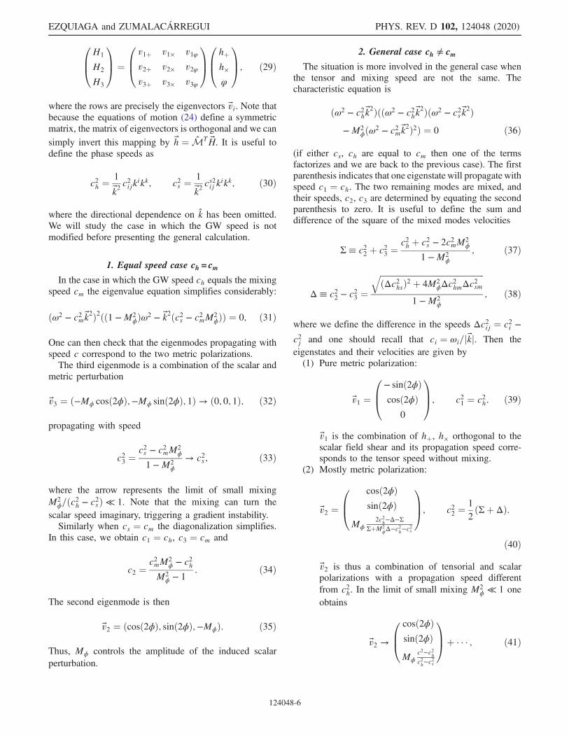
propagation direction ∇⊥ (note that we can always definekð0Þ · kð1Þ ¼ 0). The geometry of the problem is summa-rized in Fig. 2.Equation (48) can be used to compute the deflection

angle for light and ultrarelativistic particles with minimalcoupling to the metric. In that case, the effective velocityinduced by the perturbed potential Φ and Ψ (using thepreviously mention canonical normalization)

c20;effðxÞc2

¼ 1 − 2ΨðxÞ1þ 2ΦðxÞ ; ð49Þ

leads to the standard expression in terms of the metricpotential

α0 ≈Z

∇⊥ðΦþΨÞdu: ð50Þ

In the case of GR sourced by nonrelativistic matter Φ ¼ Ψand one recovers the standard result αGR ≈ 2

R ∇⊥Φdu. Intheories without GW birefringence all eigenstates aredeflected by α0.Birefringence will cause the deflection angle between

two eigenstates I, J to differ by

ΔαIJ ≈ −1

2

Zdu∇⊥Δc2IJðx; kÞjrðuÞ;u; ð51Þ

and vanishes in the limit of equal speed as expected.Typical GR deflection angles are small, on the scale ofθE ∼ arcsec

ffiffiffiffiffiffiffiffiffiffiffiffiffiffiffiffiffiffiffiffiffiffiffiffiM=1012 M⊙

pfor strongly lensed cosmologi-

cal sources. These deflections are hard to resolve even forthe most precise optical telescopes. GW detectors haverather low angular resolution that is many orders ofmagnitude lower than what it would be required to detecta different incoming direction for different polarizations(although there are ambitious projects for high resolution

GW astronomy in the next decades [27]). On the otherhand, GW detectors have excellent time resolution, makingtime delays between gravitational polarizations a muchmore robust observable.

2. Time delays

There are three independent time delays that a given lenscan imprint on the observables, Δt01, Δt12, Δt23. Each timedelay will be the sum of a Shapiro term (difference inspeeds locally) and a geometric contribution (difference intravel distance):

ΔtIJ ≡Z

du

�1

cI−

1

cJ

�þ ΔtgeoIJ ; ð52Þ

where we used the Born approximation discussed above(recall that the propagation speed will in general depend onthe position as well as the propagation direction of thesignal). Let us now discuss how the deflection angle (51)leads to the geometric time delay.Assuming a single lens and spherical symmetry, each

propagation eigenstate obeys its own lens equation

β ¼ θI − αI; ð53Þ

where β is the angular position of the source (equal for allpolarizations) and θI are the apparent position of the sourcefor each polarization I (source and lens plane, respectively),cf. Fig. 3. We have defined also αI ¼ αIDLS=DS. Here DL,DS, DLS are, respectively, the angular diameter distances tothe lens, source and between the lens and the source. In thecase of multiple lenses one should substitute the sourcewith the previous lens. The geometric time delay due to thedifferent angles (assuming cI ≈ c over the trajectory)between two propagation eigenstates can be computedfollowing the standard approach and a bit of trigonometry(see e.g., Ref. [24][Sec. IV 3]). We obtain

FIG. 2. Schematic view of the gravitational wave propagation. The undeflected GW trajectory corresponds to the solid black line foran impact parameter b, as plotted on the left. The transverse view is presented on the right together with a representation of the effect of atensor mode crossing a circle of test particles. At any given point the GW is located at a radius r and angular positions θ and ϕ.


124048-8

ΔtgeoIJ ¼ ð1þ zLÞ2c

DLDLS

DSðj αIj2 − j αJj2Þ; ð54Þ

where zL is the redshift of the lens. The order of magni-tude of the delay will be determined by the dilatedSchwarzschild diameter crossing time

tM ¼ 4GMLð1þ zLÞ=c3: ð55ÞAs a rule of thumb, one can use that tM≃10ðMLz=1M⊙Þμs,i.e., the delay is ∼months, days and minutes for lenses withMLz ¼ 1012 M⊙, 1010 M⊙, 107 M⊙, respectively. In theseunits the geometrical time delay can be written as

ΔtgeoIJ ¼ tM2ðj αIj2 − j αJj2Þ; ð56Þ

where the angles αI ¼ αI=θE are now normalized in unitsof the Einstein ring of a point lens

θE ¼ffiffiffiffiffiffiffiffiffiffiffiffiffiffiffiffiffiffiffiffiffiffiffi4GMc2

DLS

DLDS

s: ð57Þ

Assuming that the difference between the deflectionangles of the different eigenstates ΔαIJ is small comparedto the light deflection angle α0, Eq. (50), ΔαIJ ≪ α0, wefind

ΔtgeoIJ ≈ 2Δtgeo0

ΔαIJα0

; ð58Þ

where Δtgeo0 is the geometrical time delay induced by thegravitational potential on a wave propagating at the speedof light. This quantity depends on the distance to thesource, to the lens and the mass of the lens. For a point lensit is given by

Δtgeo0 ¼ tM

�DLDLS

b ·DS

��rsb

�: ð59Þ

From this expression it is explicit that the time delay issubject to the geometry of the lens source. The time delaywill be maximal when the lens is at intermediate distancesbetween the source and observer.The multimessenger and polarization time delays,

Eqs. (52), (54) constitute the most promising observablesof birefringence. Their exact values depend on the effectivebackground metric for the GWs, through the theoryparameters, lens properties and the configuration of addi-tional fields around the lens. We will now turn to thegeneral phenomenological consequences of birefringenceand its observability (Sec. IV). In Sec. VI we will study aspecific example of a theory with Vainshtein screening,with a detailed modelling of gravitational lenses.

IV. PHENOMENOLOGY ANDOBSERVATIONAL PROSPECTS

Let us now analyze the broad phenomenological con-sequences of birefringence. We will start in Sec. IVA bydescribing the observational regimes for different valuesof the time delay, with a discussion of the single andmultilens case. In Sec. IV B we will then discuss speciallensing configurations, focusing on a source near a super-massive black hole. We will address the interplay betweenbirefringence and multiple images due to strong lensing inSec. IV C. Finally, Sec. IV D addresses the probability ofdetecting GW birefringence, along with current and fore-casted constraints.

A. Observational regimes: scrambling and echoes

There are three important scales when discussing tests ofGW lensing birefringence for a given event and detectornetwork: the time resolution, the duration of the GW signaland the timescale of the observing run. Three distinctobservational regimes can be established, depending ofhow the time delay between the propagation eigenstatesΔtIJ relates to these scales.The sensitivity to ΔtIJ will be determined by modelling

as well as experimental uncertainties. For the delaybetween EM and gravitational signals, the error Δt0I islikely dominated by assumptions about the EM counter-part. For example, when the gamma ray is emitted after abinary neutron star merger. In contrast, the GW emissioncan be modeled accurately, e.g., using a post-Newtonianexpansion or numerical relativity. Thus, delays betweengravitational polarizations are mostly limited by the timeresolution of the instrument, which will be of order5

FIG. 3. Diagram of the source-lens geometry under consid-eration. The trajectory of the GW (solid black line) is curved dueto the lens with a deflection angle α. The true angular position ofthe source is β, while the observer sees the lensed image at αþ β.DL, DS, DLS are, respectively, the angular diameter distances tothe lens, source and between the lens and the source DS. b is theclosest distance of the GW to the lens.

5One can sharpen this estimate easily using a noise curve withhi → hiefΔt12 applied to each polarization, see below.


124048-9

σtg ∼ f−1peak; ð60Þ

or ∼ms for current ground detectors (LIGO/Virgo). Finally,we note that the emission of scalar polarizations is sup-pressed in many theories (due to screening mechanisms),which might make the scalar (or mostly scalar) polarizationvery hard to detect, precluding a measurement of Δt3I . Inthe following we will focus mostly on the time delaybetween the pure metric and mostly metric polarizationsΔt12.The duration of the signal Tg reflects how long a detector

is sensitive to a given event. Depending on the mass,compact binary coalescence observed by ground detectorscan last from less than a second (black hole binaries) to overa minute (neutron star binaries). Continuous signals such asrotating neutron stars (ground detectors) or mHz compactbinaries (LISA) can in principle be detected as well. In thosecases Tg is limited by the duration of the observationalcampaignTobs. Herewewill assume continuous observationup to Tobs: a more realistic analysis should account for thedetector’s duty cycle (the fact that detection are regularlyinterrupted for several reasons) when Δtij ∈ ðTg; TobsÞ.The following situations are possible:(1) Signal scrambling: if σtg ≲ jΔt12j≲ Tg the signal is

observed as a single event and time delay(s) betweendifferent eigenstates distort the waveform.

(2) Signal splitting/GW echoes: if Tg ≲ jΔt12j≲ Tobsthe signal is split and each eigenstate will beobserved as a separate event. The orbital parametersof different events will be related (e.g., orbitalinclination/orientation), and it may be possible toassociate different echoes from the same under-lying event.

(3) Single polarized signals: if jΔt12j ≳ Tobs, only oneinstance of each event can be observed. This leads toan excess of edge-on signals, relative to the expect-ation of random orientations.6

One should note that the first two effects are analogous tostrong lensing where multiple images can be produced andmight interfere if their time delay is of the order of thesignal duration (sometimes called microlensing regime).However, we stress that these are completely differenteffects in origin and are also governed by different physicalquantities (we will comment more on those differencesbelow). The scrambling and echoes are thus independent ofstrong lensing and would apply to each multiple image ifpresent. Moreover, with a large network of detectors onecould distinguish the different polarizations further distin-guishing the two effects.

In addition, multiple lenses along the line of sight willcontribute a separate time delay. Misalignment betweenlenses causes a difference in propagation eigenstates foreach subsequent lens (e.g., different angle ϕ). In thissituation, each lens causes a separate scrambling or splittingof the signal. Let us first discuss the single lens case andthen comment on the effect of multiple lenses.

1. Single lens

To better understand the effects of birefringence, let usconsider the effect of a single lens on a head-on GW event,i.e., L · n≡ cos ι ¼ 1 (this will be generalized later). In thiscase the ×;þ polarization are emitted with equal ampli-tude, and one can define the basis so that they areproportional to metric components of the 1,2 propagationeigenstates (i.e., rotating the coordinates so the azimuthalangle is ϕ ¼ 0). In this case the signal after crossing theregion where modify gravity effects are relevant is approx-imately given by

hij ≈ h×ðtÞe×ij þ hþðt − Δt12Þeþij þ � � � ; ð61Þ

where the ellipsis represent GW shadows, including thoseof additional polarizations. This relationship assumes thatthe amplitudes are approximately equal in the interactionand propagation basis, and that the mixing with the scalarmode is subdominant. While the exact relationship requiressolving the GW propagation at subleading order, ω−1, onecan assume that the corrections are small, given the largefrequency of GWs. This implies that the relative amplitudeis unchanged in the propagation so that hþ ∼ h2 andh× ∼ h1. We are also not taking into account standardlensing effects (e.g., magnifications and phase shifts). Allthese assumptions could be generalized, but for pedagogi-cal purposes we restrict the derivation to the simplestexample. One should note too that these assumptions holdfor GWs on FRW, where effects on the amplitude (αM) aremuch harder to detect than effects on the phase (αT , m2

g).The strain on a given detector is then

h ≈A×h× þAþhþ þ � � � ; ð62Þ

whereAI is the detector’s response for a given polarization,given the source’s position in the sky. Figure 4 shows theeffect of the time delay for a binary black hole signal, bothon each polarization and as seen in one detector. Thescrambling regime jΔt12j < Tg is characterized by a timemodulation of the amplitude, caused by the interferencebetween the signals, as well as two distinct imprints fromthe merger, separated by Δt12. In the splitting regime twocopies of the signal are detected with a delay Δt12 andamplitudes given by the detector’s response to eachpolarization. Multiple detectors provides further meansto characterize the signal via different response functions,time delays, etc.

6Due to duty cycle/interruptions of the detector, a fraction ofechoes are missed even if Tg ≲ jΔt12j ≲ Tobs, leading to an excessof edge-on events. Given that source binaries are randomlyinclined, knowing the antenna patter of the detector and havinga large statistical sample may allow us to discriminate this effect.


124048-10

For this example we have considered an unlensed,nonspinning, equal-mass binary. However, some of theseeffects could be degenerate with binary parameters in moregeneral systems. For example spinning, asymmetric bina-ries are known to introduce modulations in the waveform.Similarly, strongly lensed multiple GWs produce multipleimages that might have short time delays for certain lenses.Nonetheless, with a network of detectors one could use thepolarization information to break this degeneracies. Forinstance, if one expects the amplitude difference betweenthe echoes be produced by the projection on the detector’santenna pattern of each eigenstate, one could use theinformation on the sky localization to constrain thispossibility. If both polarizations can be detected independ-ently, the degeneracy can be completely broken.

2. Multiple lenses

Multiple lenses can cause further scrambling and split-ting of a GW source. Considering spherical lenses andtreating their effects as independent, the relationshipbetween the signal at the source and the detector can beapproximated as

hd ≈YL

½eiωt1M−1 expðT ÞM�Lhs: ð63Þ

Here hd;s is the vector of amplitudes in Fourier spacein the interaction eigenstates at the detector/source. Mis the mixing matrix introduced in (29), which relatesthe interaction hI, I ∈ ð×;þ;φÞ and propagation HJ;J ∈ ð1; 2; 3Þ eigenstates. Here we have also introducedthe delay matrix which encompasses the phase evolution ofthe propagation eigenstates

expðT Þ ¼

0B@

1 0 0

0 e−iωΔt12 0

0 0 e−iωΔt13

1CA; ð64Þ

(note that an overall factor eiωt1 has been factored out toexpress the results in terms of time delays). The subscript Ldenotes that the quantities depend on the lens properties(mass, mass distribution) and its configuration relative tothe line of sight (impact parameter b, azimuthal angle ϕ).Schematically, Eq. (63) is telling us that if a GW crosses

a region near a lens, the GW propagation will be deter-mined by the propagation eigenstates, possibly leading totime delays among them. Therefore, after crossing the firstlens the initial GW wave packet could be split in separatepackets for each HI. Then, if another lens is on the line ofsight, each GW packet will subdivide again since theeignestates of the second lens will be in general differentfrom the first one. In principle this process can be iteratedfor as many lenses are in the GW trajectory. A possibleobservational signature of these multiple splittings wouldbe a significant reduction in the GW amplitude since forrandom orientations of the lenses the projection into theeigenstates at each lens will reduce the overall amplitude ofthe detected signals. Of course, the key question is howprobable is to have this multiple encounters. We touch onthe lens probabilities in Sec. IV D.Before moving on, we remind the reader that Eq. (63) is

only valid at leading order and does not take into accountthe modifications of the amplitudes of the propagationeigenstates. In general both the mixing matrix and eigen-frequencies depend on the spatial coordinates. This meansthat there would be spatially dependent corrections to theamplitudes of H. This next to leading order corrections canbe computed solving at higher order in the short-wave

FIG. 4. Signatures of birefringence in the scrambling (jΔt12j < Tg, left) and the splitting (jΔt12j > Tg, right) regimes. The upperpanels show the amplitude of the two gravitational polarizations with Δt12 ¼ −0.05, 0.7s, respectively. The lower panel show the strainobserved on a LIGO-H1 detector withAþ ¼ −0.38,A× ¼ 0.71 (additional detectors in the network will have different responses). Thesignal corresponds to two 30 M⊙ black holes, head-on (cos ι ¼ 1) at 500 Mpc.


124048-11

expansion. As previously alluded, we leave this analysis forfuture work.

B. Source near the lens

A particular interesting source-lens configuration hap-pens when the GW source is very close to the lens. In thatcase, the GW will inevitably travel in a region where thebackground fields are relevant and more likely to enhancebirefringence effects. Due to this particular geometry, thetotal time delay will be dominated by the Shapiro part,since the geometrical time delay scales with the source-lensdistance DLS.A realization of this setup will occur if a binary black

hole (BBH) merge near the disk of an active galacticnucleus (AGN) (see e.g., [28]). There, compact objects areexpected to accumulate in specific regions of the accretiondisk, the so-called migration traps, at around 20 − 300rs[29]. A schematic representation of this type of systems isgiven in Fig. 5, where the impact parameter of the binary bis smaller than the typical scale r⋆ where modified gravitybackgrounds become relevant. We remind the reader thatthis scale does not have to be related with the scale of stronglensing.Recently, a possible EM counterpart to the heaviest BBH

detected so far, GW190521 [30], was announced in [31].The interpretation of this coincident EM-GWevent was thatthe BBH mergered within the disk of an AGN: the largekick after the merger would have produced the flare. Themass of the SMBH was estimated to be ∼1–10 × 108 M⊙,

meaning that the binary might have merger at only 0.0002–0.03 pc of the SMBH. Such short distance to the lens wouldmake this event a great candidate to test modifications ofgravity. It is to be noted, however, that GW190521 is alsothe furthest event so far with the largest localizationvolume, making the clear association of a counterpartmore difficult. In any case, if this BBH formation channelconstitutes a significant fraction of the observed events, onecould use this population to very efficiently constrain theGW lensing effects beyond GR discussed here. Moreover,LISA could also see the inspiral of ∼5–10 events of thisclass during a four-year mission (see e.g., Fig. 2 of [32]), inwhich case the dopler modulation and repeated lensingcould confirm the origin [33,34]. A multiband observationtogether with an identification of the flare after mergerwould make this type of BBH system a truly uniquelaboratory of the theory of gravity.The opposite scenario of a lens near the observer is also

promising to probe birefringence. One possibility is tocorrelate the maps of nearby gravitational lenses with skylocalizations of GW events: for instance, events locatedbehind galactic plane could be used to test theoriespredicting a sizeable time delay by Milky Way galaxies.These are examples of unusual lensing setups leading toobservable consequences in theories with GW birefrin-gence. In contrast, for standard lensing configurationsobservable effects are predominantly caused by interveninglenses. In the remainder of the section we will focus onintervening lenses.An examples of a test of gravity using lensing maps of

known galaxies was used after GW170817 [35]. Alter-natively, one could also look at the statistical effect of large-scale inhomogeneities [36].

C. Strong vs weak lensing and multiple images

Lensing effects depend on the source-lens geometry andcan be classified into strong and weak lensing dependingon whether multiple images form or not. These standardmultiple images are in addition to possible echoes/splittingcaused by birefringence. In particular, a point lens ischaracterized by an Einstein ring radius

rE ≈ θE ·DL; ð65Þ

where the Einstein angle θE was given in (57). Wheneverthe impact parameter of the source is of the order or smallerthan the Einstein radius, b≲ rE, we are in the regime ofstrong lensing and multiple images of the same GW couldbe produced by the lens. In the case of having differentpropagation eigenstates, multiple images of eachHI will beproduced. In the opposite limit b≳ rE we are in the regimeof weak lensing where only one image can be detected.Weak lensing modify gravity effects could be constrainedcross-correlating with galaxy surveys [37]. Note that themodify gravity lensing effects are a priori independent of

FIG. 5. Diagram of a binary black hole coalescence near asupermassive black hole (SMBH). In this situation the Shapirotime delay is the dominant effect. The binary and the lens areseparated by an impact parameter b and the GW propagates in theu direction.


124048-12

the “standard” lensing regimes. Depending of the theorythere could be large modifications even in weak lensing.This was schematically depicted in Fig. 1, where the scaleof modify gravity r⋆ does not correspond to rE.For example, a GW travelling near a point mass lens will

form two images with positive (+) and negative (−) parityfor each propagation eigenstate. For angular positionsβ ≲ 1, we can quantify the dimensionless time delayT� ¼ t�=tM between the two images analytically [38]

T− − Tþ ¼ 1

2y

ffiffiffiffiffiffiffiffiffiffiffiffiffiy2 þ 4

qþ ln

�xþx−

�; ð66Þ

where we have defined the source angle in units of theEinstein radius y ¼ β=θE and the images positions

x� ¼ 1

2

��y�ffiffiffiffiffiffiffiffiffiffiffiffiffiy2 þ 4

q ��: ð67Þ

This tells us that for source angles of the order of theEinstein radius, y ∼ 1, the delay between the images will beof the order of the characteristic lensing time scale tM,which for lenses of ∼1010 M⊙ corresponds to a delay ∼1day. If the impact parameter is much smaller than rE,y ≪ 1, the delay simplifies to T− − Tþ ∼ y, which impliesthat it will be parametrically smaller than tM. This meansthat for certain theories and lens-source geometry it ispossible that there is a degeneracy between the delay ofmultiple images and the delay between the echoes ofdifferent eigenstates.The interplay between strong lensing and the anomalous

speed lensing effects beyond GR will depend on therelation between the Einstein radius and the typical scalewhere modify gravity effect are relevant. For example, formodified gravity theories with an screening mechanism thatwe will study in Sec. VI, the relevant scale to comparewill be the Vainsthein radius rV . In the regime of weaklensing, when b ≫ θE, only one image is detectablewith a negligible magnification jμIj1=2 ≃ 1. This was ourassumption for Fig. 4, where we computed the echoes andscrambling assuming only one image.Strong lensing probabilities have been discussed in the

context of advanced LIGO-Virgo extensively [18–20] withrates ranging between 1 every 100 or 1000 events depend-ing on the source population and lens assumptions. ForLISA, it has been shown that a few strongly lensed GWfrom SMBH binaries could be observed [39], althoughthe result is highly dependent on the modeling of thepopulation of SMBHs.

D. Lensing probabilities

Let us now estimate the probabilities of observing GWbirefringence by randomly distributed lenses. We willconsider two generic dependences with the lens mass,proportional to (1) the Einstein radius and (2) a physical

radius with a power-law dependence on the lens mass.We will use these simple models to compare with currentGW data (assuming nondetection) and estimate the sensi-tivity of future observations.The probability of observing an event with a given

property X (e.g., a time delay) is [40]

PX ¼ 1 − e−τX ; ð68Þ

where the optical depth is

τX ¼ 1

δΩ

Zzs

0

dVcnðz0ÞσX: ð69Þ

Here δΩ is an element of solid angle, dV ¼ δΩD2L

dz0ð1þz0ÞHðz0Þ

is the physical volume element given a solid angle δΩ,nðz0Þ is the physical density of lenses and σX is the angularcross section. We will assume all lenses have equal massand dilute as matter, with physical number density

nðz0Þ ¼ ΩL3H2

0

8πGMLð1þ z0Þ3: ð70Þ

The lens mass distribution and other properties can beincluded straightforwardly in Eq. (69). Note that the

prefactor can be written as 3H20

8πGML¼ ð4π

3r3Þ−1 in terms of

a characteristic scale

r≡�2GML

H20

�1=3

≈ 1.2 Mpc

�ML

1012 M⊙

�1=3

: ð71Þ

Here r is the mean separation between lenses if theUniverse’s critical density was distributed in objects ofmass ML. Incidentally, r coincides with the Vainshteinradius for the theory studied in Sec. VI for parametersΛ4 ¼ H0, p4ϕ ¼ 1.The angular cross section σX represents the area around a

lens for which a propagation effect X is observable, wherewe take that

σX ¼ πθ2X; ð72Þ

i.e., effects are detectable for angular deviations ≤ σX awayfrom a lens. This form assumes spherical symmetry andthat the effects are easier to detect closer to the lens, as it isexpected for example from modify gravity screeningbackgrounds. If the effect X becomes undetectable for asmaller angle θ0 (e.g., transitioning from the scramblingto the echoes regime) then the cross section would beσX ¼ πðθ2X − θ20Þ instead. We will analyze two simple casesfor θX.As a first case, let us assume detectability at a fraction of

the Einstein radius


124048-13

θEX ¼ αXθE; ð73Þ

where αX depends on the theory, but not on redshift or lensmass. The optical depth then reads

τEX ¼ 3

2ΩLα

2X

Zzs

0

dz0ð1þ z0Þ2Hðz0Þ=H0

H0DLDLS

DS; ð74Þ

and is independent of mass, which is a known property oflensing probabilities for pointlike lenses and sources. Massdependence often arises from more detailed modeling, e.g.,finite source size [41] or extended lenses producingmultiple detectable images [40].For comparison, let us also consider detectability below a

given impact parameter around the lens

θphX ¼ RX

DL

�M

1012 M⊙

�n; ð75Þ

where n characterizes the mass dependence and RX isdetectable radius for typical galactic lenses, which dependsonly on the parameters of the theory. The optical depth isthen

τphX ¼ ΩLh�

RX

22 kpc

�2�M=M⊙

1012

�2n−1 Z zs

0

dz0ð1þ z0Þ2Hðz0Þ=H0

:

ð76Þ

This dependence is general enough to include scalings likethe Einstein radius [n ¼ 1=2, but without the redshiftdependence, cf. Eq. (74)], the Schwarzschild radius(n ¼ 1, as in theories with scalar hair) or the Vainshteinradius (n ¼ 1=3, as in massive gravity or Horndeski

theories cf. Sec. VI). In the rest of this section we willassume that all the mass is effectively in lenses of 1012 M⊙.However, note that for n < 1=2 the contribution of lighterlenses can be significantly enhanced, cf. Vainshtein radiusscaling in Sec. VI, Eq. (152).The dependence in the source redshift differs between

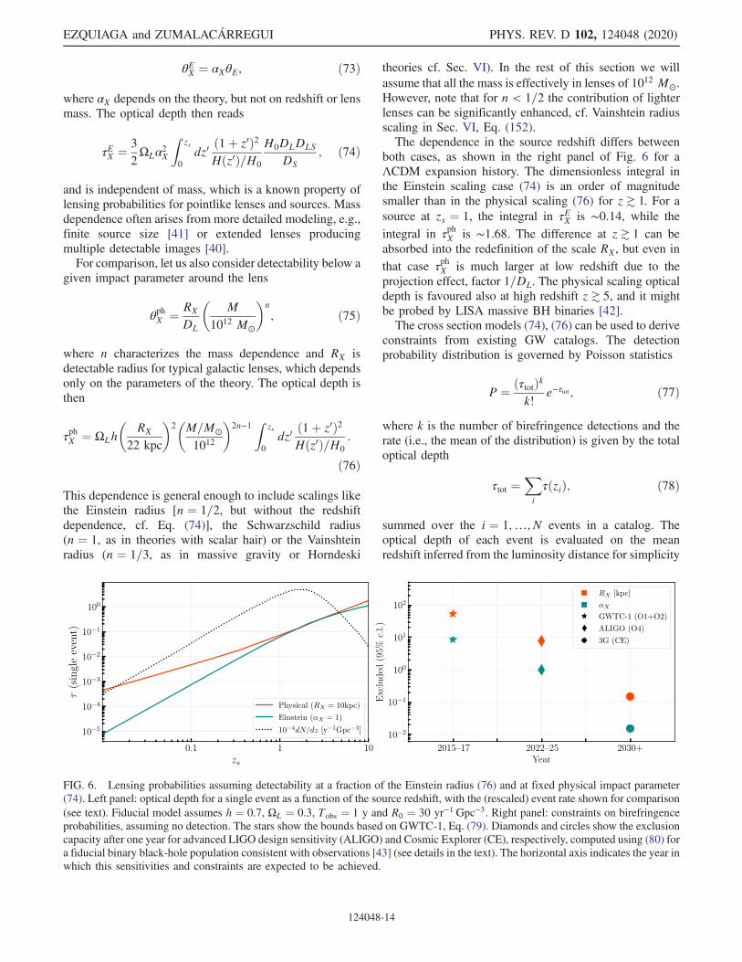
both cases, as shown in the right panel of Fig. 6 for aΛCDM expansion history. The dimensionless integral inthe Einstein scaling case (74) is an order of magnitudesmaller than in the physical scaling (76) for z≳ 1. For asource at zs ¼ 1, the integral in τEX is ∼0.14, while theintegral in τphX is ∼1.68. The difference at z≳ 1 can beabsorbed into the redefinition of the scale RX, but even inthat case τphX is much larger at low redshift due to theprojection effect, factor 1=DL. The physical scaling opticaldepth is favoured also at high redshift z≳ 5, and it mightbe probed by LISA massive BH binaries [42].The cross section models (74), (76) can be used to derive

constraints from existing GW catalogs. The detectionprobability distribution is governed by Poisson statistics

P ¼ ðτtotÞkk!

e−τtot ; ð77Þ

where k is the number of birefringence detections and therate (i.e., the mean of the distribution) is given by the totaloptical depth

τtot ¼Xi

τðziÞ; ð78Þ

summed over the i ¼ 1;…; N events in a catalog. Theoptical depth of each event is evaluated on the meanredshift inferred from the luminosity distance for simplicity

FIG. 6. Lensing probabilities assuming detectability at a fraction of the Einstein radius (76) and at fixed physical impact parameter(74). Left panel: optical depth for a single event as a function of the source redshift, with the (rescaled) event rate shown for comparison(see text). Fiducial model assumes h ¼ 0.7, ΩL ¼ 0.3, Tobs ¼ 1 y and R0 ¼ 30 yr−1 Gpc−3. Right panel: constraints on birefringenceprobabilities, assuming no detection. The stars show the bounds based on GWTC-1, Eq. (79). Diamonds and circles show the exclusioncapacity after one year for advanced LIGO design sensitivity (ALIGO) and Cosmic Explorer (CE), respectively, computed using (80) fora fiducial binary black-hole population consistent with observations [43] (see details in the text). The horizontal axis indicates the year inwhich this sensitivities and constraints are expected to be achieved.


124048-14

(uncertainty of the recovered redshift can be included).Current constraints can be derived assuming nondetection(k ¼ 0) in the GWTC-1 of LIGO/Virgo O1þ O2 sources[44]. The total optical depth (78) evaluated on the models(74), (76) can be translated via Poisson statistics into

αX < 8.5

RX < 53 kpcð95%C:L:Þ ð79Þ

forΩL ¼ 0.3, h ¼ 0.7. We note that this limit is subject to adetailed analysis of the waveforms in GWTC-1, to con-fidently exclude birefringence effects. As we will see,future observing runs and next generation detectors canincrease these bounds significantly.In order to estimate the potential of future GW obser-

vations we consider the predicted total optical depth

τtot ¼Z

dzdλτðzÞ dNdz

; ð80Þ

where the differential event rate is given by

dNdz

¼ Rðz; λÞ Tobs

1þ zdVc

dzPdetðz; λÞ: ð81Þ

Here λ collectively determines all additional source proper-ties (besides redshift), Pdet is the detection probability,

Rðz; λÞ is the event rate (per comoving volume) and dVcdz ¼

4πDAðzÞ2ð1þzÞHðzÞ ð1þ zÞ3 is the comoving volume factor (physical

volume times density factor). Equation (78) is recoveredsetting dN

dz ¼P

i δðz − ziÞ.The predicted total optical depth (80) can be used to

estimate how future surveys can improve existing bounds(79). We take as a reference model of sources a populationof BBHs consistent with GWTC-1 [43]. Specifically wetake a power-law distribution of primary masses pðm1Þ ∼m−1.6

1 between 5 and 45 M⊙ with a redshift evolution of themerger rate following the star formation rate [45][Eq. 15]normalized to R0 ¼ 30 yr−1 Gpc−3. We set the detectionthreshold at a signal-to-noise ratio of 8 for a single detector.These predictions applied to LIGO O2 sensitivity are ingood agreement with the results from GWTC-1, Eq. (79).Figure 6 shows the expected bounds on αX, RX after a

year of observation with ALIGO design sensitivity andCosmic Explorer (CE) third-generation technology,together with the current bounds (79). The horizontal axisindicates the expected year when these projections could beachieved. In particular, ALIGO design sensitivity isexpected to be achieved during the next observing runO4. Current constraints can be expected to improve anorder of magnitude by O4, and two orders of magnitudeafter one year of Cosmic Explorer and other third gen-eration ground-based detectors. Note that bounds on thetotal cross section are quadratic in αX, RX, so the actual

sensitivity increases by ∼2, 4 orders of magnitude,respectively.The framework introduced in this section applies exclu-

sively to a homogeneous and random distribution of lenses.It is important to note that in certain situations the locationof the lens relative to the source might not be random andthus these results may vastly underestimate the probabil-ities. Examples include when the lens is near the observer(GW events located behind the Galactic Center) or whensources forms very close to the lens (stellar mass BHbinaries in the vicinity of a massive black hole) as discussedin Sec. IV B.

V. PROPAGATION EIGENSTATES INHORNDESKI THEORIES

As a particular set up, we will concentrate in gravitytheories adding just one extra propagating degree of free-dom with respect to GR. We will restrict to those scalar-tensor theories with covariant second order EOM. Viableextensions are known [46–48] but more complex to analyzebecause of higher derivatives, and some classes induce arapid decay of GWs into fluctuations of the scalar field[49,50]. This naturally leads us to Horndeski’s gravity [51],whose action reads [52]

S½gμν;ϕ� ¼Z

d4xffiffiffiffiffiffi−g

p �X5i¼2

Li þ Lm

�; ð82Þ

with

L2 ¼ G2ðϕ; XÞ; L3 ¼ −G3ðϕ; XÞ□ϕ; ð83Þ

L4 ¼ G4ðϕ; XÞRþ G4;Xðϕ; XÞ½ð□ϕÞ2 − ϕμνϕμν�; ð84Þ

L5 ¼ G5Gμνϕμν −

1

6G5;Xðϕ; XÞ½ð□ϕÞ3

− 3ϕμνϕμν□ϕþ 2ϕμ

νϕναϕα

μ�: ð85Þ

This theory has four free function Gi of the filed ϕ andits first derivatives −2X ¼ ϕμϕ

μ. Here and for the restof the paper we adopt the following notation for thecovariant derivatives of the scalar field: ϕμ ≡∇μϕ andϕμν ≡∇μ∇νϕ.We will divide the analysis of this large class of theories

in two. First, we will consider the subclass of theories inwhich the causal structure of the propagating tensor modesis determined by the background metric. Thus, in theseluminal theories the phase evolution of GWs is equal to thatof light (Sec. VA). Then, we will consider nonluminaltheories in which the tensor modes have a different causalstructure (Sec. V B).The causal structure of GWs in Horndeski gravity over

general space-times in the absence of scalar waves has beenstudied in [53]. For the subset of luminal theories, the


124048-15

propagation without scalar waves was investigated in [54],while a geometric optics framework including φ wasdeveloped in [55]. The study of GWs, considered as abackground space-time, revealed that scalar perturbationscan become unstable in Horndeski theories [56], a difficultythat affects even luminal theories such as kinetic gravitybraiding, Eq. (99). In addition, there has been large effortsto study the GW propagation over cosmological and BHspace-times. We refer the interested reader to the recentreview [1].Since the GW and scalar wave evolution will in general

depend on the propagation direction for an anisotropicbackground, it is useful to decompose the spatial compo-nents of the background tensors in terms of the directionsparallel and perpendicular to the propagation trajectory ofthe GW, defined by the wave vector ki. Specifically, wedecompose the spatial gradient of the scalar background as

ϕi ¼ ϕki þ ϕ⊥

i ; ð86Þ

so that in the transverse gauge

ϕi∇i ¼ ϕik∇i and ϕihij ¼ ϕi⊥hij: ð87Þ

These identities will be handy in what comes next.

A. Luminal theories

Since the evolution equations are coupled in general(even at leading order in derivatives), the first step is todiagonalize them. Depending of the complexity of thetheory, the diagonalization can be done covariantly. Indeed,we will see in this section that this is the case for thoseHorndeski theories with a luminal GW propagation speed.Before that, it is useful to recall the case of GR, where

one also needs to diagonalize the propagation in order toobtain a wave equation for each polarization. Although inGR there is no additional scalar field, we can effectivelytreat the trace as an additional degree of freedom. Startingfrom Einstein’s equations, one can see that the tensor EOMof the linear perturbations,

δGμν ¼ δRμν −1

2hμνR −

1

2gμνδR;

¼ −1

2□hμν þ∇ðμ∇αhνÞα −

1

2gμν∇α∇βhαβ

−1

2∇μ∇νhþ 1

2gμν□hþOð∇hÞ ¼ 0; ð88Þ

include a mixing with the trace at leading order inderivative, where Oð∇hÞ captures terms linear or lowerorder in derivatives. The way to diagonalize these equationsis to redefine the tensor perturbation to

hμν ≡ hμν −1

2gμνh ð89Þ

(which are well known as trace-reversed metric perturba-tions [22]). In this way, after fixing the transverse gauge onthe new perturbations∇νhμν ¼ 0, one recovers the standardwave equation

δGμν ¼ −1

2□hμν þ Rμανβhαβ ¼ 0: ð90Þ

Note that, at face value, this equation is telling us that thepropagation eigenstates of GR are a combination of thetensor perturbations and its trace. In vacuum we can alwaysfix the trace to zero (so that hμν ¼ hμν), but in the presenceof matter its value has to be computed.The fact that in GR only the TT perturbations are

nonzero in vacuum can also be easily derived solvingthe constraint equations. In particular, the 00 Einsteinequation tell us that Ψ ¼ 0, the 0j that wi ¼ 0 and thespatial trace that Φ ¼ 0. We are left then with the ijequations which lead to only two independent equations forhþ and h×.Horndeski theories with a luminal GW speed will share

with GR the structure of the second order differentialoperator acting on the tensor perturbations. Such operatorcorresponds to

Dαβμν ≡ −

1

2□δμαδνβ þ∇ðα∇μδνβÞ −

1

2gαβ∇μ∇ν: ð91Þ

The fact that this operator contains the wave operator pluslongitudinal terms makes the GW-cone and light-coneequal, and thus cg ¼ c in the absence of φ [53].In the following we will generalize this procedure to

gravitational theories with luminal GW propagation: gen-eralized Brans-Dicke, kinetic gravity braiding [57] and theunion of both.

1. Generalized Brans-Dicke

A pedagogical exercise is to consider a generalizedBrans-Dicke type scalar-tensor theory described by anaction

S ¼Z


p ðG4ðϕÞRþ G2ðXÞÞ; ð92Þ

which introduces a direct coupling between the scalar fieldand the second derivatives of the metric through G4ðϕÞ. Atleading order in derivatives, the metric EOM for the linearperturbations are given by

Dμναβhαβ þG4ϕðgμν□φ −∇μ∇νφÞ þOð∇h;∇φÞ ¼ 0;

ð93Þ

where for convenience we have already introduced thetrace-reversed metric and the differential operator (91), andwe encapsulate all lower/nonderivative terms which are not


124048-16

relevant for this calculation in Oð∇h;∇φÞ. Thus, there is amixing of the perturbations, which also occurs in the scalarEOM (see Appendix B for more details). We can decoupleboth equations by introducing a new tensor perturbation

hμν ≡ hμν −G4;ϕ

G4

gμνφ ð94Þ

combining both the trace-reversed and scalar perturbations,which is a well-known result in the literature (see e.g.,[58]). After applying the transverse gauge condition on thenew field ∇μhμν ¼ 0, the EOM simplify to

−1

2G4□hμν þOð∇h;∇φÞ ¼ 0; ð95Þ

Gαβs ∇α∇βφþOð∇h;∇φÞ ¼ 0; ð96Þ

where Gαβs is the effective metric for the scalar perturbations

Gαβs ¼

�6G2

4;ϕ

G4

þ 2G2X

�gαβ − 2G2XXϕ

αϕβ: ð97Þ

Therefore, the propagating eigenstates are a combination ofthe original metric and the scalar perturbations. At thisorder in derivatives and in the absence of sources, the scalarwaves will only be present if they are initially emitted.Moreover, because φ multiplies gμν, the scalar perturbationwill generically contribute to the trace of the tensorperturbations. We can see this explicitly when solvingthe constraint equations for the nonradiative d.o.f.,obtaining

Ψ ¼ −Φ ¼ G4ϕ

2G4

φ; wi ¼ 0: ð98Þ

Thus, in Brans-Dicke-type theories, the scalar perturbationexcites the scalar polarizations of the metric leaving anadditional pattern in the GW detector [59,60].7 Noticeably,in this theory there is no mixing of the radiative tensorialDoF hþ;× with the scalar φ (Gþ;×s ¼ 0), so hþ;× becomedirectly the propagation eigenstates traveling at the speedof light.

2. Kinetic gravity braiding

Similarly, we can also diagonalize the propagationequations of kinetic gravity braiding (KGB),

S ¼Z


p ðG4R − G3ðXÞ□ϕÞ ð99Þ

a cubic Horndeski theory with a direct coupling betweenthe derivatives of the metric and the scalar field throughG3ðXÞ. Note that for simplicity we have fixed G4 ¼ const,although one could easily add a scalar field dependence likein the previous section. Because of this cubic coupling, themetric EOM display a mixing of the scalar and tensorperturbations,

Dμναβhαβ þG3;Xðϕμϕν□φ − 2ϕαϕðμ∇νÞ∇αφ

þ gμνϕαϕβ∇α∇βφÞ þOð∇h;∇φÞ ¼ 0: ð100Þ

At this order of derivatives, we can diagonalize theequations by changing variables to8

hμν ≡ hμν −G3;X

G4

ϕμϕνφ: ð101Þ

As in the case of Brans-Dicke theory, once we apply thetransverse condition to the new tensor perturbation hμν, theEOM reduce schematically to Eqs. (95)–(96) (see details onthe form of the effective metric for the scalar fieldperturbations in Appendix B). Accordingly, the maindifference between KGB and Brans-Dicke theories is thatthe propagation eigentensor involves the scalar perturbationvia the gradients of its background field. In other words,depending on the background, the scalar mode couldcontribute to other polarizations different from the trace.We can see this excitation of non-TT d.o.f. directly by

solving the constraint equations. For example, if the scalarbackground has only temporal components, ϕμ ¼ ϕ0δ

0μ, the

nonradiative d.o.f. read

Ψ ¼ Φ ¼ G3Xϕ20

4G4

φ; wi ¼ 0; ð102Þ

and hþ;× propagate independently of φ. On the oppositeregime, if ϕμ ¼ ð0;ϕiÞ, we obtain that

Ψ ¼ G3Xjϕkj24G4

φ; ð103Þ

wi⊥ ¼ −iG3XϕkG4

ϕi⊥k

∇0φ; ð104Þ

Φ ¼ G3Xðjϕj2□þ 3jϕ⊥j2∇0∇0Þ4G4k2

φ: ð105Þ

Moreover, for the radiative d.o.f., we find that the mixingwith the scalar has the same causal structure that the tensormodes,

7It is to be noted an analogous sourcing of the gravitational(nonradiative) potentials occurs over cosmological backgrounds,see e.g., Ref. [61] [Eqs. 3.17–3.21] in the limit k ≫ H.

8To the best of our knowledge, this metric perturbationdiagionalizing KGB equations is novel in the literature.


124048-17

Ghh ¼ □; Gþ;×s ¼ −G3Xϵ

þ;×μν ϕμϕν

4G4

□: ð106Þ

We are then in the ch ¼ cm case discussed in Sec. III A 1,meaning that both hþ;× will be propagating eigenstatesmoving at the speed of light. On the other hand, the scalareigenstate will be a combination of the original scalar φ andthe tensor modes hþ;×

3. Luminal Horndeski gravity

Altogether, the most general luminal Horndeski theorywould be a combination of the previous cases

S ¼Z


p ðG4ðϕÞR − G3ðϕ; XÞ□ϕþ G2ðϕ; XÞÞ:

ð107Þ

The dependence in ϕ in G2 and G3 does not affect thediagonalization of the leading derivative terms in the EOM.Because we are solving for the linear perturbations, theEOM can be diagonalized by a linear combination of theprevious field redefinitions, i.e.,

hμν ≡ hμν −G4;ϕ

G4

gμνφ −G3;X

G4

ϕμϕνφ: ð108Þ

This field redefinition is reminiscent of a disformal trans-formation [46,62–64], e.g., the linearized version of themanipulations presented in Ref. [65]. We note that thisresult agrees with Eq. (40) of [66].

B. Nonluminal theories

As we increase the order of derivatives of the couplingsbetween the metric and the scalar, we enter on the realm ofnonluminal Horndeski theories: theories in which thesecond order differential operator acting on hμν no longercorresponds to the one of GR, Dμν

αβ, Eq. (91). This inducesa different causal structure in the effective GW metriccompared to the one that EMwaves are sensitive to, leadingto cg ≠ c [53], even in the absence of scalar perturbationsφ. These theories involve higher order Horndeski functionswith derivative dependence G4ðXÞ and G5ðϕ; XÞ.Moreover, in this class of theories, the same couplings

that produce an anomalous propagation speed induce abackground dependent polarization mixing. Specifically,this mixing can be seen in the EOM from the contraction ofperturbed Riemann tensors with first ϕμ or second deriv-atives ϕμν of the scalar field. Therefore, depending on thescalar field profile the polarizations of the metric maychange as they propagate. In practice, this makes theanalysis of the propagating d.o.f. difficult in a covariantapproach.

1. Quartic theories

A good example representing this phenomenology is ashift-symmetric quartic Horndeski theory

S ¼Z


p ðG4ðXÞRþG4;Xðð□ϕÞ2

− ϕμνϕμνÞ þ G2ðXÞÞ; ð109Þ

where we have added a generalized kinetic term for thescalar. The leading derivative EOM for the tensor and scalarperturbations are then

G4Dμναβhαβ þG4;XδRμανβϕ

αϕβ

þ ðG4;XCμναβ þG4;XXEμναβÞ∇α∇βφ

þOð∇h;∇φÞ ¼ 0; ð110Þ

and

Gαβs ∇α∇βφþ 2G4;Xϕ

μνDμναβhαβ

− 2G4;XXϕμνδRμανβϕ

αϕβ þOð∇h;∇φÞ ¼ 0; ð111Þ

where δRμανβ is a second order differential operatorconstructed by a linear combination of the perturbationsof the Riemann tensor, Cμναβ and Eμν

αβ are backgroundtensors made of second derivatives of the scalar profile andGαβs is the effective metric for the scalar perturbations which

depends on KX and G4;X (see full definitions inAppendix B). It is precisely the presence of δRμανβ whichinduces the nonluminal propagation. Note also that eitherG4;X ≠ 0 or G4;XX ≠ 0 triggers the mixing of the perturba-tions in both equations.In the following we will concentrate in the simplest

theory producing this effect, a quartic theory linear in X.9 Itis clear from the Eqs. (110)–(111) that the dimensionlesscoupling controlling the mixing is

ϒ ∼ðlnG4Þ;X

Gs∇∇ðϕ=MPlÞ; ð112Þ

where X ¼ X=M2Pl and we have introduced Gs, which

quantifies the value of jGαβs j, to ensure canonical normali-

zation of the scalar field. In other words, if Gs is large, thescalar perturbations decouple from the GW evolution.We now identify the propagation eigenstates of the

quartic theory using two methods: (1) perturbative solutionfor small mixing and (2) diagonalization based on a local3þ 1 splitting.Perturbative solutions for ϒ ≪ 1.—In order to gain

some intuition, we will consider first situations in which

9Theories with G4 ¼ fðϕÞX are equivalent to quintic theorieswith G5ðϕÞ up to a total derivative [67].


124048-18

the GW-scalar mixing is small, ϒ ≪ 1, so we can make aperturbative expansion of the propagation equations. Thuswe expand the full solution as

hμν ¼ hð0Þμν þ hð1Þμν þ hð2Þμν þ � � � ; ð113Þ

φ ¼ φð0Þ þ φð1Þ þ φð2Þ þ � � � ; ð114Þ

solving order by order iteratively.Accordingly, at leading order (LO), we have to solve

simply

G4□hð0Þμν ¼ 0; ð115Þ

Gαβs ∇α∇βφ

ð0Þ ¼ 0; ð116Þ

where we have already applied the transverse condition

∇μhð0Þμν ¼ 0. Therefore, at LO, the equations decouple andwe can fix the TT gauge, hð0Þ ¼ 0. As a consequence, ifthere is no initial scalar wave φð0ÞðteÞ, it will remain zero

along the propagation. One can also see that while hð0Þμν

propagate at the speed of light, φð0Þ can have a nonluminalvelocity.At next-to-leading order (NLO), the mixing terms arise

in the equations

G4□hð1Þμν þ G4;Xϕαϕβ∇α∇βh

ð0Þμν − 2G4;XCμναβφ

ð0Þαβ ¼ 0;

ð117Þ

Gαβs ∇α∇βφ

ð1Þ −G4;Xϕμν□hð0Þμν ¼ 0; ð118Þ

where we have set ∇μhð1Þμν ¼ 0. Note that, since hð0Þμν is TT,

G4;Xϕαϕβ∇α∇βh

ð0Þμν is the only nonzero term from

−2G4;XδRð0Þμανβϕ

αϕβ, where δRð0Þμανβ indicates that the per-

turbations of the Riemann tensors are with respect to the

zeroth order tensor perturbation hð0Þμν . Consequently, theNLO equations tell us that φð1Þ is only sourced if ϕμν

TT ≠ 0.Moreover, one can also see that, when there is no initialscalar wave, the second term of the tensor equation (117)acts to modify the GW propagation speed. This can be

shown explicitly by solving hð1Þμν with its Green function and

noting how the propagator of the total solution hNLOμν ¼hð0Þμν þ hð1Þμν is modified. In the opposite situation, whenφð0ÞðteÞ ≠ 0, the different propagation speed of the scalarwave introducing a dephasing in the mixing. Note however

that even in the absence of an initial scalar wave, hð1Þμν is notnecessarily TT.At next order, the equations contain all their possible

terms,

G4□hðnÞμν − 2G4;XδRðn−1Þμανβ ϕαϕβ − 2G4;XCμναβφ

ðn−1Þαβ ¼ 0;

ð119Þ

Gαβs ∇α∇βφ

ðnÞ − G4;Xϕμν□hðn−1Þμν ¼ 0; ð120Þ

so they are valid for any n > 1 (again ∇μhðnÞμν ¼ 0).Local, general solution in the 3þ 1 splitting.—

Although the general solution when the mixing is domi-nant, ϒ ∼ 1, is not analytically tractable, we can obtaingeneral solution in a local region of space-time wherelinearized gravity applies. This is equivalent to going toRiemann normal coordinates. We have to solve theevolution and constraint equations for the 11 d.o.f.of the problem, sij, φ, Ψ, wi and Φ [see Eq. (12)]. Asbefore, we will work in the spatially transverse gauge,∂isij ¼ ∂iwi ¼ 0, which it is always possible to choose.Moreover, for clarity in the equations, we will restrictto a static, spatially dependent scalar field background,ϕμ ¼ ð0;ϕiðxÞÞ. Additional details on the equations for thisderivation are given in Appendix C.Let us focus for the moment on the case of a quartic

Horndeski theory in the absence of scalar perturbations. Inthat case the leading derivative EOM are given by (110).Thus, essentially, we need to compute the different com-ponents of δGμν and δRμανβϕ

αϕβ. For reference, oneshould remember that in GR there is only δGμν present.As in GR, the 00 equation,

2G4∇2Ψþ G4Xðϕiϕi∇2Ψþ ϕiϕj∂i∂jΨÞ ¼ G4Xϕ

iϕj∇2sij;

ð121Þ

provides a constrain equation forΨ. The difference is thatΨis sourced by ϕiϕjsij, even in vacuum.We can proceed similarly for the other equations. For the

0j equations, we obtain the constraint equation for wj as

∇2wj −G4X

G4

ð2ϕkϕl∂k∂ ½jwl� − ϕjϕk∇2wkÞ

¼ 4∂0∂jΨþ 2G4X

G4

ðϕjϕk∂0∂kΨþ ϕkϕ

k∂0∂jΨ

− 2ϕkϕl∂0∂ ½jsl�kÞ: ð122Þ

In the GR limit we recover the case that wi is sourced by Ψand consequently it vanishes in vacuum. Here, the newfeatures are the couplings to the backgrounds as well as thedependence on sij.Next we move to the trace of the ij equations which

yields an equation for the last nonpropagating perturbationΦ, i.e.,


124048-19

2∇2Φþ G4X

G4

ðϕiϕi∇2Φþ ϕiϕj∂i∂jΦÞ ¼ 2∇2Ψ − 6∂2

0Ψ

−G4X

G4

ðϕiϕjð∂0∂iwj − ∂20sijÞ þ ϕiϕ

ið4∂20Ψ − 2∇2ΨÞÞ:

ð123Þ

In the GR limit Φ is only sourced by Ψ. Therefore, for thesame reason as before, in vacuum both vanish. However,for quartic Horndeski Φ is sourced by Ψ, wj and sij.In conclusion, we have solved Ψ, Φ and wj in the

transverse gauge (∂isij ¼ 0 and ∂jwj ¼ 0) in terms of sij,which are the two transverse-traceless components. Wedenominate these nonradiative, nonzero perturbations GWshadows. We can obtain the equations for sij plugging inthese solutions for the nonpropagating perturbations in thespatial tensor equations, cf. (C13)–(C14).In order to take into account the scalar perturbation φ we

have to both incorporate the new terms in the tensorequations and include the scalar EOM. Because we areexpanding over flat space, the second derivatives of thescalar background are purely spatial ϕ0μ ¼ 0. We alsomake the further assumption that G4XX ¼ G4XXX ¼ 0.Then, the new contribution to the tensor equations is

G4XAμνφ ¼ G4Xðð□ϕ□ − ϕαβ∇α∇βÞgμν −□ϕ∇μ∇ν

− ϕμν□þ 2ϕðμα∇α∇νÞÞφ: ð124Þ

For the 00 equation, we have

G4XA00φ ¼ −G4Xð□ϕ∇i∇i − ϕij∇i∇jÞφ: ð125Þ

Then, Ψ can be solved in terms of sij and φ. For the 0jequations we add

G4XA0jφ ¼ G4Xð−□ϕ∇0∇j þ ϕjk∇k∇0Þφ: ð126Þ

Similarly, wj can be solved in terms of sij and φ once Ψ issubstituted. For the ij equations

G4XAijφ ¼ G4Xðð□ϕ□ − ϕkl∇k∇lÞδij −□ϕ∇i∇j

− ϕij□þ 2ϕðik∇k∇jÞÞφ: ð127Þ

This allow us to compute the spatial trace

G4XAijδijφ ¼ G4Xð−2□ϕ∇0∇0 þ□ϕ∇i∇i − ϕkl∇k∇lÞφ:

ð128Þ

From this last equation we can solve Φ in terms of sij andφ. Finally, we also have the scalar equation

Gαβs ∇α∇βφþ 2G4Xϕ

ijδGij ¼ 0: ð129Þ

Once we solve the constraints, we end up with twoindependent equations from the ij equations plus the scalarEOM for three DoF, hþ, h× and φ. Therefore, we havesolved the constraint equations.For simplicity we present the equations at linear order in

G4X, where they follow the structure of Sec. III A withcoefficients

G4Ghh ¼ G4□þ G4Xjϕkj2∇i∇i; ð130Þ

2G4Gþs ¼ G4XðϕijϵijþÞ□; ð131Þ

2G4G×s ¼ G4Xðϕijϵij×Þ□; ð132Þ

4G4Gss ¼ Gαβs ∇α∇β: ð133Þ

Nonlinear terms modify the mixing coefficients G×s andGþs but preserve Ghh. In this way we can solve thepropagation diagonalizing the EOM as described inSec. III A. In the absence of mixing, the propagationspeeds for the tensor modes is

c2h ¼ 1þG4Xjϕkj2G4

; ð134Þ

which also coincides with the speed of the tensorialpropagation eigenstate c1 ¼ ch. On the other hand, thescalar speed without mixing reads

c2s ¼ 1 −G2XXjϕkj2

G2Xð135Þ

in the limit where G4XX ¼ G4XXX ¼ 0 (a more generalexpression can be derived from the full equations in [65]).One should note that inhomogeneous GW speed (134)generalizes the result of [53,68] where φ was set to 0 and aTT gauge was assumed without solving the constraintequations. This result agrees with the radial and angularspeed obtained from the calculation of the small-scaleperturbations around a BH in Horndeski gravity [69] andgeneralizes that result to arbitrary propagation direction.Finally, we have to remember that although nonpropa-

gating, Ψ, Φ and wj cannot be set to zero. At leading orderin G4X they read (assuming propagation in z direction)

2G4Ψ ¼ G4Xðϕiϕjsij þ ðϕ⊥ÞiiφÞ; ð136Þ

kG4wx ¼ 2iG4X∇0ðϕxϕzhþ þ ϕyϕzh× þ ϕxzφÞ; ð137Þ

kG4wy ¼ 2iG4X∇0ðϕxϕzh× þ ϕyϕzhþ þ ϕxzφÞ; ð138Þ

2k2G4Φ ¼ G4Xð∇0∇0ð2ϕiϕjsij þ δijðϕij − ϕ⊥ij=3ÞφÞ

þ k2ϕiϕjsijÞ: ð139Þ


124048-20

This suggests that all the tensor polarizations will beexcited and that the fact that there are only 3 d.o.f. canbe seen from the correlations among the differentpolarizations. GW detectors can in principle detect theseGW shadows.

2. Quintic theories

Quintic Horndeski theories also feature GW-scalarmixing at leading order in derivatives that cannot bediagonalized covariantly. In fact, the interactions have anincreased level of complexity. In addition to the operatorsin (110)–(111), there will be, for example, contractions ofthe perturbations of the Riemann tensor with secondderivatives of the scalar background ϕμν. Because thescalar second derivative tensor could have differentprojections into the GW polarizations eþμν and e×μν,propagation effects are subject to polarization depend-ence. In particular, even in the absence of scalar waves, itis possible for the GW speed to depend on the polari-zation in a generic quintic Horndeski model. For in-stance, operators like

ϕiϕjϕkl□hkl ¼ 2ϕiϕjðϕþ□hþ þ ϕ×□h×Þ ð140Þ

would introduce such a birefrengent effect.An interesting exception is scalar Gauss-Bonnet gravity

(SGB) [70], where due to the symmetry of the theory thetensor speed does not depend on the polarization [71]. Thistheory is the described by the Lagrangian

L ¼ R2−1

2∇aϕ∇aϕ − VðϕÞ þ fðϕÞGB; ð141Þ

where GB ¼ R2 − 4RabRab þ RabcdRabcd is the Gauss-Bonnet invariant. After a bit of calculus, one can showthat in the absence of scalar waves, the leading orderequations for SGB are the same that for a quartic theory ifone replaces

ϕμϕν=M2Pl → fμν ≡ fϕϕϕμϕν þ fϕϕμν; ð142Þ

M2PlG4X

G4

→ G≡ 16

M2Pl − 16fαβgαβ

: ð143Þ

Then, locally and at leading order, one obtains the pro-pagation velocity

c2h ¼ 1þ 16fkM2

Pl

¼ 1þ 16ðfϕϕuu þ fϕϕjϕkj2Þ

M2Pl

; ð144Þ

which is the same for both polarizations. It is to be noted thathere ϕuu corresponds to the projection of the secondderivatives of the scalar field background in the directionof propagation. Therefore, the novelty in the propagation

speed of GWs in SGB compared to a quartic Horndeskitheory is precisely this dependence in the second derivatives.We can go one step further and compute the mixing of

the GWs with scalar waves at leading order in derivative ina vacuum solution (RB ¼ RB

μν ¼ 0). The EOM would looklike

δGμν þ GδRμανβfαβ þ 4fϕRBμανβφ

αβ ¼ 0; ð145Þ

□φþ 2fϕRμανβB δRμανβ ¼ 0; ð146Þ

where δG and δRμανβ are the perturbations of the Einsteinand Riemann tensor respectively defined in Appendix B.From these equations we can see that the main difference ofthe mixing in SGB and quartic Horndeski is that in theformer the mixing is through the curvature backgroundwhile in the latter this happens through the scalar fieldbackground. We leave the analysis of the detectability ofthe mixing of GWs and scalar waves in SGB for futurework.

VI. PROBING GW PROPAGATIONIN SCREENED REGIONS

In this section wewill present detailed GW lensing predic-tions for a concrete Horndeski theory featuring Vainshteinscreening. We first introduce the theory Lagrangian andparameters, as well as some quantities of interest. InSec. VI A we present the local solutions of the scalar fieldaround spherical lenses, including screening phenomena.Section VI B briefly describes the cosmological behaviorand limits imposed by compatibility with the GW speedon the cosmological background following GW170817. InSec. VI C we present detailed predictions for the multi-messenger and birefringent time delays for pointlike lenses.Section VI D explores the emergence of GW shadows forsignals propagating in a screened region. Finally, Sec. VI Ediscusses the prospects to further probe Horndeski theoriesusing GW lensing and birefringence.To exemplify this modified GW propagation due to

screening, let us come back to a quartic Horndeski theory(see Sec. V B 1). We will consider a linear coupling to thecurvature of the form

L ¼ Lshift-sym þ p4ϕϕMPlR; ð147Þ

where the shift-symmetric quartic theory Lshift-sym is givenby (109) in which the free functions Gi depend only onthe derivatives of the scalar. This linear coupling can bethought as the leading order term of an exponentialcoupling ep4ϕϕ=MPl , which in the Einstein frame correspondsto a linear coupling to the trace of the energy-momentumtensor.For concreteness, we will consider a polynomial expan-

sion in the Horndeski parameters


124048-21

G2 ¼ M2Pl

�2p2XX þ p2XX

X2

Λ22

�; ð148Þ

G4 ¼M2

Pl

2

�1þ 2p4ϕϕþ 2

XNn¼1

p4Xn

�−XΛ24

�n�: ð149Þ

Note that we are measuring the field in Planck unitsϕ ¼ ϕ=MPl so that X ¼ X=M2

Pl. Each of these terms havean associated energy scale Λn which determines the lengthscale at which nonlinearities become relevant. We candefine the nonlinear length scale

ðr4Þ3 ¼rs2Λ2

4

; ð150Þ

associated to the quartic theory, and

ðr2Þ2 ¼rsΛ2

; ð151Þ

associated to the scalar kinetic interaction. Here rs ¼ 2GMis the Schwarzschild radius.

A. Local background

Screening mechanisms suppress fifth forces aroundmassive objects, so that GR holds in their vicinity. Thisis achieved in different ways depending on the underlyingtheory [72], but typically it is caused by a particularbackground configuration preventing the propagation ofscalar modes (fifth forces). These backgrounds can beinduced by the local matter density or curvature profile,depending on the screening mechanism. Screened envi-ronments are natural setups for GW lensing beyondGR, since they introduce nontrivial background profilesaround massive objects that could modify the GWpropagation. GW lensing effects beyond GR are thusexpected to be different for different types of screeningmechanisms.For the quartic theory under consideration, screening is

caused by nonlinear derivative self-interactions of the scalarfield. Screening becomes effective within a scale known asthe Vainshtein radius:

rV ≡ p1=34ϕ r4 ¼

�p4ϕGM

Λ24

�1=3

ð152Þ

(assuming p4Xn ¼ 1 in the last equality). Whenever thecoupling to matter p4ϕ is of order one, the nonlinear scale(150) corresponds to the Vainshein radius. The linearizedfield equation is valid for r ≫ rV : in that unscreened regionthe scalar field mediates a force ∼p2

4ϕ times that of gravity.It will be convenient to measure distances in units of

the nonlinear scale of the quartic theory: r ¼ r=r4. Inthis units, following [73], we can obtain the screening

background from the dimensionless quantity xðrÞ, whosealgebraic equation for this theory is given by10

ðp2X þ 3p24ϕÞx − 6p4Xp4ϕx2 þ ðp4XX þ 2p2

4XÞx3¼ −p4ϕMðrÞ=r3; ð153Þ

where MðrÞ accounts for the mass enclosed in a sphere ofradius r, i.e., MðrÞ≡ 4πM−1

Rr0 ð−Tt

tÞr2dr. To isolate thedependence on the source mass distribution, we make thedefinition

∂ϕ∂r ¼ 1

2rrsxðrÞ≡ rs

∂ϕ∂r : ð154Þ

This is a convenient rewriting of the local scalar fieldbackground because all the dependence in the lens massis isolated in the prefactor rs, while ∂ϕ=∂r is a profiledepending only on the parameters of the theory. Forexample, outside of the source but well within the screeningradius, r ≪ rV , the profile becomes constant

∂ϕ∂r

��r≪rV

→ −1

2

�p4ϕ

p4XX þ 2p24X

�1=3

ð155Þ

and far from the source we recover the decay with theinverse square distance

∂ϕ∂r

��r≫rV

→ −1

2

p4ϕ

p2X þ 3p24ϕ

1

r2: ð156Þ

As it is evident from the above equation, p4ϕ indeedweights the coupling to matter. One should note that bydifferentiating (153) along the radial direction one can alsoobtain an algebraic equation for ∂2ϕ=∂r2 as a function ofthe theory parameters and ∂ϕ=∂r. This is useful forinstance to compute the second derivative backgroundlimit within the screening region.We have seen previously that the coupling of the scalar

perturbation to the tensorial radiative modes is supportedby the second derivatives of the scalar background [recallEq. (111)]. For a radial scalar configuration the secondorder partial derivatives read

ϕ;ij ¼ ϕ00 xixjr2

þ ϕ0

r

�δij −

xixjr2

�; ð157Þ

using r ¼ffiffiffiffiffiffiffiffiffiffiffiffiffiffiffiffiffiffiffiffiffiffiffiffiffix2 þ y2 þ z2

p. The projection to spherical

coordinates [x ¼ r sinðθÞ cosðϕÞ, y ¼ r sinðθÞ sinðϕÞ,z ¼ r cosðθÞ] yields the following projections (see Fig. 2)

10To link with the notation of [73] one can set μ ¼ β ¼ 0,ξ ¼ p4ϕ, η ¼ 2c2, α ¼ −p4X and ν ¼ p4XX, as well asAðrÞ ¼ MðrÞ=r3.


124048-22

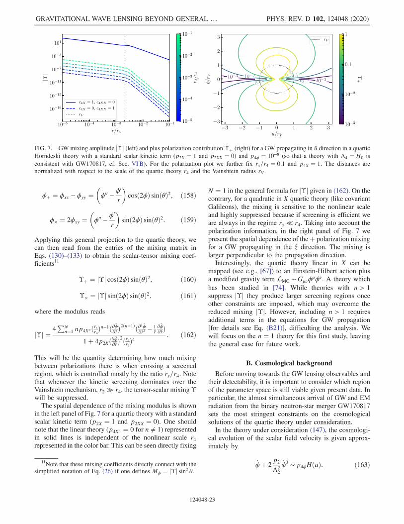
ϕþ ¼ ϕxx − ϕyy ¼�ϕ00 −

ϕ0

r

�cosð2ϕÞ sinðθÞ2; ð158Þ

ϕ× ¼ 2ϕxy ¼�ϕ00 −

ϕ0

r

�sinð2ϕÞ sinðθÞ2: ð159Þ

Applying this general projection to the quartic theory, wecan then read from the entries of the mixing matrix inEqs. (130)–(133) to obtain the scalar-tensor mixing coef-ficients11

ϒþ ¼ jϒj cosð2ϕÞ sinðθÞ2; ð160Þ

ϒ× ¼ jϒj sinð2ϕÞ sinðθÞ2; ð161Þ

where the modulus reads

jϒj ¼4P

Nn¼1 np4Xnðrsr4Þn−1ð

∂ϕ∂rÞ

2ðn−1Þð∂2ϕ∂r2 −1r∂ϕ∂rÞ

1þ 4p2Xð∂ϕ∂rÞ2ðr2r4Þ4

: ð162Þ

This will be the quantity determining how much mixingbetween polarizations there is when crossing a screenedregion, which is controlled mostly by the ratio rs=r4. Notethat whenever the kinetic screening dominates over theVainshtein mechanism, r2 ≫ r4, the tensor-scalar mixingϒwill be suppressed.The spatial dependence of the mixing modulus is shown

in the left panel of Fig. 7 for a quartic theory with a standardscalar kinetic term (p2X ¼ 1 and p2XX ¼ 0). One shouldnote that the linear theory (p4Xn ¼ 0 for n ≠ 1) representedin solid lines is independent of the nonlinear scale r4represented in the color bar. This can be seen directly fixing

N ¼ 1 in the general formula for jϒj given in (162). On thecontrary, for a quadratic in X quartic theory (like covariantGalileons), the mixing is sensitive to the nonlinear scaleand highly suppressed because if screening is efficient weare always in the regime rs ≪ r4. Taking into account thepolarization information, in the right panel of Fig. 7 wepresent the spatial dependence of theþ polarization mixingfor a GW propagating in the z direction. The mixing islarger perpendicular to the propagation direction.Interestingly, the quartic theory linear in X can be

mapped (see e.g., [67]) to an Einstein-Hilbert action plusa modified gravity term LMG ∼Gμνϕ

μϕν. A theory whichhas been studied in [74]. While theories with n > 1suppress jϒj they produce larger screening regions onceother constraints are imposed, which may overcome thereduced mixing jϒj. However, including n > 1 requiresadditional terms in the equations for GW propagation[for details see Eq. (B21)], difficulting the analysis. Wewill focus on the n ¼ 1 theory for this first study, leavingthe general case for future work.

B. Cosmological background

Before moving towards the GW lensing observables andtheir detectability, it is important to consider which regionof the parameter space is still viable given present data. Inparticular, the almost simultaneous arrival of GW and EMradiation from the binary neutron-star merger GW170817sets the most stringent constraints on the cosmologicalsolutions of the quartic theory under consideration.In the theory under consideration (147), the cosmologi-

cal evolution of the scalar field velocity is given approx-imately by

_ϕþ 2p2

Λ22

_ϕ3 ∼ p4ϕHðaÞ: ð163Þ

FIG. 7. GW mixing amplitude jϒj (left) and plus polarization contribution ϒþ (right) for a GW propagating in u direction in a quarticHorndeski theory with a standard scalar kinetic term (p2X ¼ 1 and p2XX ¼ 0) and p4ϕ ¼ 10−8 (so that a theory with Λ4 ¼ H0 isconsistent with GW170817, cf. Sec. VI B). For the polarization plot we further fix rs=r4 ¼ 0.1 and p4X ¼ 1. The distances arenormalized with respect to the scale of the quartic theory r4 and the Vainshtein radius rV .

11Note that these mixing coefficients directly connect with thesimplified notation of Eq. (26) if one defines Mϕ ¼ jϒj sin2 θ.


124048-23

This relation is exact for an exponential coupling G4 ¼expðp4ϕϕÞ in a matter-dominated universe (cf. Ref. [75][Eq. (42)]), but reduces to the theory at hand when p4ϕ ≪ 1

and the contributions ofG4;X are negligible compared to theG2 terms. It also provides a good order-of-magnitudedescription for the late Universe in the presence of acosmological constant. If the canonical kinetic term domi-nates, the scalar is cosmologically unscreened and itsvelocity reads

_ϕ ∼ p4ϕH if ð _ϕ ≪ Λ2=ffiffiffiffiffip2

p Þ; ð164Þ

whereas _ϕ ∼ ðp4ϕHΛ22=2p2Þ1=3 if the noncanonical term

dominates ( _ϕ ≫ Λ2=ffiffiffiffiffip2

p), corresponding to the cosmo-

logically screened regime. In what follows we will assumethe unscreened solution (164).For a quartic theory (149) the cosmological change in

GW speed at z ∼ 0 reads

αT ¼ 4G4;XX ¼Xn

4np4Xn

�−p24ϕH

20

2Λ24

�n

; ð165Þ

where the last equality assumes the unscreened cosmo-logical solution (164). Assuming that only one among thep4Xn coefficients is nonzero

αT ∼�p4ϕH0

Λ4

�2n; ð166Þ

where we have set c4Xn ¼ 1, as it is redundant with Λ4 inthis case. Then the GW170817 constraint jαT j≲ 10−15

gives a relation between the two theory parameters. For aquartic theory linear in X (n ¼ 1), this bound can besatisfied for sufficiently small matter couplings comparedto the scale of the theory, i.e.,

p4ϕ ≲ 10−8Λ4=H0: ð167Þ

The suppression of modified gravity effects ensures that theapproximations used to estimate the cosmological evolu-tion (164) remain valid if Λ4 ≳H0. If Λ4 ≲H0, quarticHorndeski gravity breaks down as an effective field theoryat energy scales comparable to GWs with typical LIGO/Virgo frequencies [76].As we will see below, GW lensing and birefringence

effects can extend constraints based on the GW speed overthe cosmological background, Eq. (167). The reasonbehind it is that the scalar field gradient sourced by amassive lens is significantly larger than the cosmologicaltime variation ϕ0= _ϕ ≫ 1 in a region much larger than theVainshtein radius. We will use this fact to approximate_ϕ ∼ 0 to compute GW propagation, i.e., considering staticlenses hereafter.

C. Time delays

One of the main GW propagation observables is the timedelay between different propagation eigenstates and withrespect to a possible EM counterpart. For that, we need tocompute first the propagation speeds. Assuming that theGW propagates in the u direction, using Eq. (134), weobtain the propagation speed of the tensor modes in theabsence of scalar waves

c2h ¼ 1 − 2 cos2 θM2

Pl

G4

Xn

np4Xn

�rsr4

�n�∂ϕ∂r

�2n

; ð168Þ

which tends to the speed of light when rs ≪ r4 and/orθ → π=2. This velocity also corresponds to the one of thepurely tensorial propagation eigenstates, c1 ¼ ch, whenthere is mixing. In the absence of mixing, the scalar speed isgiven by Eq. (135) to arrive at

c2s ¼ 1þ 2 cos2 θM2

Pl

G2

p2XX

�r2r4

��∂ϕ∂r

�2

; ð169Þ

which tends to the speed of light when r2 ≪ r4 orp2XX → 0.When there is mixing but ϒ is small, the speeds of the

propagation eigenstates are

c21 ¼ c2h; ð170Þ

c22 ¼ c2h þ jϒj2 sin4 θ ðΔc2hÞ2

Δc2hsþ � � � ; ð171Þ

c23 ¼ c2s − jϒj2 sin4 θ ðΔc2sÞ2

Δc2hsþ � � � ; ð172Þ

where we have defined the difference in the speed withrespect to the speed of light Δc2i ¼ c2i − c2 and amongdifferent eigenstates Δc2IJ ¼ c2I − c2J. The dots refer tohigher order terms in the expansion in jϒj.We can now compute the associated time delays between

different signals. As discussed in Sec. III B, there will betwo contributions: the Shapiro and the geometrical timedelay. We discuss them separately before commenting ontime delays between multiple images in strong lensing.

1. Shapiro time delay

The Shapiro time delay between the tensorial eigenstateand an EM counterpart, in the limit of small velocitydifference Δc2h=c2 ≪ 1, is

Δt10 ¼Z

du

�1

ch−1

c

�¼

Zdu

�−Δc2h2c3

þ � � ��; ð173Þ

where, again, u is the GW propagation direction. On theother hand, the difference between the two mostly tensorialpolarizations, in the limit of Δc221=c2h ≪ 1, is


124048-24

Δt21 ¼Z

du

�1

c2−

1

c1

�¼

Zdu

�−Δc2212c3h

þ � � ��;

¼Z

du

�−jϒj2sin4θðΔc2hÞ2

2Δc2hsc3hþ � � �

�: ð174Þ

We see then that for a small mixing jϒj ≪ 1 the time delaybetween the mostly tensorial eigenstates will be suppressedcompared to the time delay of the fastest mode and thespeed of light. We can observe this directly in Fig. 8, wherewe present the difference in the speed and associated timedelays. Now, because the multimessenger time delay Δt10scales with the scalar background ∂ϕ=∂r, which becomesconstant in the inner screened region, the delay saturates atimpact parameters smaller than the Vainshtein radius. Wefind this precisely in the blue line of Fig. 9. On the hand, forthe tensorial polarization delays, because the delay is also

proportional to jϒj2 sin4 θ, the delay increases as a functionof the impact parameter. This is shown in the red line. Wethen conclude that for impact parameters much smaller thanthe screening radius the delay between the tensorialeigenstates Δt21 becomes more constraining that the multi-messenger delay Δt10. Nonetheless, such close encountersare less probable (cf. Sec. IV D).Going to the particular quartic theory studied in this

section, we can see that the multimessenger time delayscales as

dthdz

∼ 2 cos2 θXn

np4Xn

�rsr4

�n�∂ϕ∂r

�2n

: ð175Þ

Since the scalar field profile decays rapidly outside of thescreened region, determined by rV ∼ p1=3

4ϕ r4, the order ofmagnitude of the delay will be given essentially by rV timesthe ratios ðrs=r4Þnð∂ϕ=∂rÞ2n, where we can find the scalingof the scalar background in (155). For a theory withG4 linearinX we can compute the order of magnitude of the maximumtime delay

Δthjmax ≲ p4ϕ

p1=34X

2GML

c3;

∼ 1 s

�1

p4X

�1=3

�p4ϕ

10−4

��ML

1010 M⊙

�: ð176Þ

The time delay thus increases with the coupling to matter p4ϕ

and the lens mass. We could also integrate analytically for u,b ≪ rV , since we know the solution of ∂ϕ=∂r, to obtain

Δthju;b≪rV ≃�rsr4

��p24ϕ

4p4X

�1=3�u − b · atan

�ub

��; ð177Þ

where the integration is performed from −u to u.This order of magnitude calculation can be compared

with the explicit calculation that we present in the left panelof Fig. 10 as a function of the parameter space p4ϕ and Λ4

for a supermassive black hole (modeled as a point lens) ofmass 1010 M⊙. We emphasize that our results can be easilyadjusted to other masses. It is important to note though thatfor larger masses (galactic order of magnitude) one wouldexpect the mass to be distributed in a halo, so that the pointlens approximation is broken. Introducing a realistic massdistribution would reduce the mass contained in the innerscreened region, reducing the induced time delay. We willelaborate more on this later in Sec. VI E. Finally, let usmention that for the multimessenger time-delay Δt10 therewould be an astrophysical uncertainty of order 1–10 sec-onds. This means that in practice one can only rule outmodify gravity theories with larger delays.We can also compute explicitly the time delay between

the polarization eigenstates. Starting from (174) and notingthat for our fiducial theory cs ¼ c (so that Δc2hs ¼ Δc2h),we find

FIG. 9. Shapiro crossing time delay induced by a point mass ofM ¼ 1010 M⊙ in a theory with p2X ¼ −p4X ¼ 1, p2XX ¼ p4XX

and p4ϕ ¼ 10−8Λ=H0 as a function of the impact parameter b inunits of the nonlinear scale of the quartic Horndeski theory r4.

FIG. 8. Difference in the speed between the metric eigenstateand light (blue) and the two mostly metric eigenstates (red) as afunction of the impact parameter b in units of the scale of thequartic Horndeski theory r4. The solid and dashed-dotted linesevaluate the speed at different points of the trajectory u. For thisexample we have chosen p4ϕ ¼ 10−8, Λ4 ¼ H0, p4X ¼ −1 andp2X ¼ 1.


124048-25

dt21dz

∼ jϒj2 sin4 θ dthdz

: ð178Þ

This means that Δt21 will be suppressed with respect toΔth. From Fig. 9 we see that Δt21 increases inverselyproportional to the impact parameter b. We can alsocompute the time delay analytically close to the lens

Δt21ju;b≪rV ≃1

4p34X

�p4ϕ

p4XX þ 2p24X

�4=3 rs

r4·atanðz=bÞb=ðr4Þ2

;

ð179Þwhich in this case will dominate the overall integral sincethe major part of the delay is accumulated close to the lens.Nonetheless, one should remember that smaller values of bare less probable to occur. For that reason we fix b ¼ rV tocompute the time delays in the right panel of Fig. 10.Thanks to the Δt21 ∼ 1=b scaling, this plot can easily beadapted to other choices of the impact parameter. Oneshould remember that the detectability of the birefringencetime delay is only limited by the time resolution of GWdetectors that can be considered to be ∼ms.

2. Geometrical time delay

In order to compute the geometrical time delay (54), wefirst need to obtain the deflection angle associated to eachpropagation eigenstate, which can be obtained from theirpropagation speed (48). In particular, the deflection anglebetween the tensor propagation eigenmode and the speed oflight is given by

Δα10 ¼ −1

2

Zdur4

sin θ∂Δc210∂r ;

¼ 4p4X

�rsr4

�Zdur4

sin θcos2θ∂ϕ∂r

∂2ϕ

∂r2 ; ð180Þ

where in the second line we have specialized for a quartictheory linear in X. This corresponds to the blue line inFig. 11, where one can see that inside the screened regionthe deflection angle difference decreases with the impactparameter.We can similarly compute the deflection angle between

the two mostly tensorial propagation eigenstates

Δα21 ¼ −1

2

Zdur4

sin θ∂Δc221∂r ;

¼ −1

2

Zdur4

sin5θ

�2jϒj ∂jϒj

∂r Δc210 þ jϒj2 ∂Δc210

∂r�:

ð181Þ

This corresponds to the red line in Fig. 11. In this case, thedeflection angle is dominated by the behavior close tothe lens. This can be approximated analytical solving the

FIG. 10. Shapiro time delays between the purely tensor eigenstate with speed c1 ¼ ch with respect to the speed of light c, Δt10 (left),and among the two mostly tensor polarizations Δt21 (right), as a function of the parameter space of the coupling to matter p4ϕ and theenergy scale of the theory Λ4. We plot the time delay accumulated after crossing the screened region of a point lens of 1010 M⊙ with animpact parameter b ¼ rV. The gray shaded region is the part of the parameter space already ruled out by the cosmological time delay inconfrontation with GW170817.

FIG. 11. Deflection angle induced by a point mass of M ¼1010 M⊙ in a theory with p2X ¼ −p4X ¼ 1, p2XX ¼ p4XX andp4ϕ ¼ 10−8Λ4=H0 as a function of the impact parameter b inunits of the scale r4 of the theory.


124048-26

integral in the limit u, b ≪ rV . For our fiducial theory weobtain

Δα21 ¼16 · 22=3

105p2=34ϕ p1=3

4X

�rsr4

��rVb

�2

: ð182Þ

From this expression the most important feature is that itscales with the inverse of the square of the impactparameter. This growth is faster than the typical 1=binduced by a gravitational potential, as can be seencomparing with the black solid line in Fig. 11. One cansee though that for impact parameters of the order of theVainshtein radius the difference in the deflection angle issmall compared to the effect of the point mass potential.Using (54) we can translate the difference in the

deflection angles into the geometrical time delay. As wehave seen in Fig. 11, the difference in the deflection anglewill be much smaller than the deflection angle induced bythe gravitational potential (except very close to the lenswhere the difference reduces). Therefore we can use theapproximate expression for the geometrical time delaygiven in Eq. (58) that makes use of this hierarchy in theorder of magnitude of the deflection angles.The mass of the lens and its relative location in the line of

sight determine the relative importance of the Shapiro andgeometric contributions to the total time delay. In Fig. 12we present the ratio of both time delays as a function of thelens redshift. The geometrical time delay dominates forlenses halfway to the source, while Shapiro dominateswhen zL → 0, zS. With fixed b ∼ rV , this is driven by theproportionality with the universal deflection angle α0 ∝r2E=b in Eq. (58), as r2E ∝ DLDLS is reduced when the lensis near the source or the observer.The Shapiro-to-geometric contribution depends differ-

ently on lens mass in multimessenger and birefringentdelays (different line styles, left panel of Fig. 12). TheShapiro contribution to Δt21 is reduced with increasing

mass, while the opposite is true for Δt10, independently ofthe lens redshift. The mass dependence can be understoodfrom the right panel of Fig. 12, where we present how theVainshtein radius compares to the Einstein radius as afunction of the scale of the theory for fixed αT ¼ 10−16. ForΛ4 ¼ H0, as chosen in the left panel, a lens with 1010 M⊙will have the Vainshtein radius well within the stronglensing region, while a 105 M⊙ lens will have rV > rE.Whenever the impact parameter is smaller than rE, thegeometrical time delay will be large. On the other hand, themultimessenger Shapiro delay scales with the Vainshteinradius and decreases faster than the geometrical one whenthe lens mass is reduced. Finally, the birefringent Shapirodelay is mostly accumulated near the lens and thus is lessaffected by the reduction of the lens mass than theanalogous geometrical delay.

3. Multiple image time delays

As introduced in Sec. IV C, in the regime of stronglensing there will be multiple images with an associateddelay between them. At the same time, each of this imageswill be subject to the effects of Shapiro and geometricaltime delay for the propagation eigenstates. It is thereforeappropriate to ask how this multiple image time delayscompare to the delay between the propagation eigenstates.For the example screening theory that we are considering

here, we have seen in the right hand plot of Fig. 12 thatindeed the Vainshtein radius falls inside the Einstein radiusfor a sector of the parameter space. At small impactparameters, the time delay between the images scales asΔt� ∼ tM · b=rE while the Shapiro time delay between themostly tensor polarization scales as Δt21 ∼ tM · rV=b.Therefore, depending on the value of b, the time delaybetween the images could be larger than the one betweenthe eigenstates or vice versa. Note that in terms of statisticsΔt� > Δt21 is much more probable, as it corresponds tolarger impact parameters. Therefore, if a pair of GWs were

FIG. 12. On the left, comparison of the Shapiro and geometrical time delays (evaluated at the Vainshtein radius) as a function of thelens redshift for a fixed source at zS ¼ 1. On the right, ratio of the Vainshtein and Einstein radius as a function of the scale of the quarticHorndeski theory. In both panels we consider different point lens masses.


124048-27

identified as strongly lensed images of the same event, thiswould be a perfect candidate to look for additional lensingeffects due to screening.

D. Polarization mixing and GW shadows

At leading order in the GW propagation, the other mainobservable is the appearance of additional polarizationsbeyond the transverse-traceless tensorial modes. We haveshown that there are two ways in which extra polarizationcan arise: (i) by a direct mixing between the tensor-scalarperturbations through ϒ and (ii) by background profilesinducing non-radiative polarizations, what we have calledGW shadows.For the propagating scalar polarizations, we can quantify

the coupling of the tensor-scalar mixing from the mostlytensor eigenvector. In particular, the third entry v23 in themixing matrix (29) informs us of the amplitude of the scalarmode that would be generated even if initially there isno scalar mode. In the top panel of Fig. 13 we plot thistensor-scalar mixing. For a linear quartic theory with astandard scalar field kinetic term, the mixing simplifies to

v23 ¼ −jϒj sin2 θ: ð183ÞWe can observe that the amplitude of the scalar perturbationcan only be sizable near the lens.With respect to the shadows polarizations, we can take

as an example the nonpropagating polarization Ψ. Inparticular, we consider a þ polarized GW propagating inthe z direction. Then, the amplitude is given by

Ψ ∼G4X

G4

�∂ϕ∂r

�2

sin2 θhþ; ð184Þ

where the approximate equality accounts for the fact that weare neglecting the contribution from φ (that as we have just

seen is small if initially φ is not sourced). Because of thesin2 θ proportionality, the amplitude of Ψ evolves similarlyto v23, as shown in the lower panel of Fig. 13, however theamplitude is many orders of magnitude smaller. Therefore,for this class of theories compatible with GW170817detecting GW shadows seems out of reach.

E. Observational prospects

To conclude this section we will discuss the observa-tional prospects of detecting these novel lensing effectsbeyond GR. The first question would be in which systemsthese effects would be relevant. In our calculations we havedone two important assumptions: we have worked atleading order in geometric optics and modeled the lensesas point masses. Both effects limit the lenses available totest quartic Horndeski theories. We will comment on theimplications of these assumptions and then discuss thepotential of GW birefringence to probe our example theory.Working in the geometric optics regime imposes a lower

limit on the frequency of GWs for which the short-waveexpansion (18), (19) applies. The exact limit depends on thebackground solution around the lens and theory-specificlower-order corrections to the propagation equations. Evenneglecting beyond GR corrections, the frequency range isrestricted by the diffraction limit inGR, belowwhich lensingmagnification becomes very inefficient. The GR diffractionlimit, Eq. (23), corresponding to GW wavelengths largerthan or comparable to the Schwarzschild radius of the lensand is shown in Fig. 15 for f ∼ Hz and kHz.The diffraction limit excludes stellar-mass lenses to test

birefringence using a short-wave expansion. This would beexcellent lens candidates, as most stellar objects can beconsidered pointlike, i.e., their sizes are much smaller thantheir Vainshtein radii, even for theories compatible withGW170817, cf. Fig. 15. Note that the validity of geometricoptics is a limit on the framework, indicating the need of awave-optics description. In particular, it does not mean thatbirefringence or time delays cease to exist. If a descriptionsimilar to the wave-optics integral is valid at low frequen-cies (Eq. 3 of [38]), the birefringence time delay shouldleave an imprint on the waveforms, even if gravitationalmagnification is negligible.The point-mass assumption is a good description for

impact parameters larger than the lens size. Becausebirefringence is suppressed beyond rV , ideal lenses shouldbe smaller than their own Vainshtein radii. Effects ongeneral lenses can be computed given their mass distribu-tion. By Gauss’s theorem, the scalar field profile around aspherically symmetric lens is sourced by the enclosed massat a given radius, i.e., MðrÞ in Eq. (153). We will modelextended sources as truncated singular isothermal spheres(SIS)

ρSIS ∼ r−2ðr ≤ RSISÞ; ð185Þ

FIG. 13. On the top tensor-scalar mixing v23 as a function of thepropagation direction u normalized by the scale r4. On the bottomshadow scalar polarization Ψ induced by an incoming hþpolarized GW in the u direction.


124048-28

and ρSIS ¼ 0 for R > RSIS. The truncation at RSIS ensures afinite total mass, but does not affect the results for lowimpact parameter. The SIS profile is widely used as a modelfor simple gravitational lenses. Note that the matter densitydiverges at the center.12

The reduced enclosed mass at low radii flattens thederivatives of the scalar field, lowering the time delays inextended lenses. Figure 14 shows the Shapiro time delaysfor two lenses with 1010 M⊙: one with a pointlike dis-tribution and another one with a SIS profile truncated atRSIS ≈ 250 kpc. The delay between gravitational polar-izationsΔt12 is more affected than the multimessenger timedelay Δt01 due to the different dependence on the scalarfield derivatives, including the shear via ϒ. This reducesboth the slope and the amplitude of Δt12.The maximum time delay in finite lenses occurs at a

parameter impact smaller than the nominal Vainshteinradius. The reason is that only the total mass with a radiusr contributes to the scalar field profile. This motivates thedefinition of an effective Vainshtein radius reffV satisfying

rVðMðreffV ÞÞ ¼ reffV ; ð186Þ

where thedependence on theory parameters has been omitted.For the truncated SIS, the mass dependenceM ∝ r results inreffV ¼ r3=2V =R1=2

SIS . For a point lens the effective and nominalVainshtein radius are equal since the enclosed mass M isconstant. Note that nonsingular lenses may have no solutionsto Eq. (186), indicating that no screening occurs.

The requirement of lenses being smaller than theireffective Vainshtein radii limits the type of objects (orportions thereof) that can contribute significant time delays.Figure 15 shows the sizes and masses of known astro-nomical objects that could act as lenses. These are, in orderof increasing mass, the Sun, a large star η Car A, a denseglobular cluster M75, the massive black hole Sgr* in thecenter of the milky way, the very dense dwarf galaxy M85-HCC1, the supermassive black hole in M87, the MilkyWayhalo and the Galaxy Cluster “El Gordo.” The mass profilesof extended objects have been extrapolated inward assum-ing a SIS distribution (185) using the total mass and size (oroutward using the central density in the case of M75). Thisextrapolation suggests that some portion of extended lenseswill be within its own effective Vainshtein radius, at leastfor theories compatible with GW170817 with low Λ4.Supermassive black-holes (SMBHs) appear as the opti-

mal lenses to further constrain quartic Horndeski theories.But because black hole solutions have vanishing Riccicurvature, SMBHs would not source the field via theconformal coupling (147) in the specific theory underconsideration. SMBHs could still provide an effective lensif they lead to the accumulation of dark matter around theblack hole with sufficient density. In such scenarios, a “darkmatter spike” could encompass a mass comparable to thatof the central black hole in a very small central region ofradius r ∼ 0.1ðMSMBH=106 M⊙Þ pc [77], sourcing thescalar field profile at the level to render the lens efficient.A coupling to the SMBHs may be induced by thecosmological evolution of the field, as it has been shownto occur for cubic Galileons (unconstrained by GW170817)[78–80].

FIG. 14. Effect of extended lenses. Lines show the Shapiro timedelays as a function of the impact parameter for a point lens(solid) and a singular isothermal profile (dashed) truncated atRSIS ¼ 250 kpc (185), both with the same mass 1010 M⊙. Thebirefringence time delay Δt12 (thick red) is more suppressed thanthe multimessenger delay Δt01 (thin blue). Vertical lines denotethe nominal Vainshtein radius (solid), the SIS effective Vainshteinradius (dashed) and the size of the lens (dotted), see text.

FIG. 15. Masses and sizes of prototypical lenses. The Vain-shtein radius is shown for example theories compatible withGW170817. The Einstein radius assumes that the lens and thesource are at cosmological distances rE ∼ 0.03 pc

ffiffiffiffiffiffiffiffiffiffiffiffiffiffiM=M⊙

p.

Shaded regions correspond to the onset of wave effects (23)for GWs frequencies ∼kHz, Hz, where geometric optics is notapplicable. Markers show the physical size of known objects (seetext). Gray lines show the enclosed mass of extended objectsassuming an isothermal profile (185).

12A regular value of the central density will suppress beyond-GR effects near the center. In the case of a homogeneous densityρðrÞ ∼ const, ϒ ∼ 0 and birefringence effects vanish entirely.


124048-29

We summarize the parameter space of the quarticHorndeski theory that could be constrained with lensingtime delays in Fig. 16. As an order of magnitude estimate,we consider testable multimessenger time delays Δt10 >1 s and delays between the polarizations Δt21 > 1 ms. It isclear from the plot that a large new sector of the parameterspace p4ϕ, Λ4 could be probed beyond current constraintsfrom GW170817. For reference we also highlight theparameter space in which the scale of the effective fieldtheory cutoff is smaller than LIGO frequencies [76].Moreover, one can also see that the birefringent Shapirotime delay can constrain a larger portion of the theory thanthe multimessenger delay, as can be seen comparing theorange and blue shaded regions, respectively.We also include the geometrical time delay induced by

the modified deflection angle with dashed and dashed-dotted lines for the multimessenger and birefrengentdelays, respectively. We have chosen the redshift of thelens to give the maximum delay and, in this case, it can bemore constraining than the Shapiro delay. One should notethat while the geometrical time delay is subject to the lens-source-observer geometry, the Shapiro delay only caresabout how close to the lens the GW passes. This means thatfor example if the lens is very close to the observer orsource, the Shapiro time delay will dominate over thegeometrical. This is interesting because from the skylocalization of the source we can then ask for instancewhether the GW has traveled close to the center of theMilky Way or Andromeda and quantify what would be theassociated Shapiro delay.The possibility of detecting Shapiro time delays via

birefringence allows novel tests of GR via GW lensing.

One such possibility is the case of a binary merging inthe environment of a SMBH, discussed in Sec. IV B. If itturns out that there is non-negligible population of BBHsmerging near an AGN, these would be ideal sources toconstrain this type of modify gravity theories. For example,if the EM flare associated to GW190521 [30] wasconfirmed as an indication of this type of systems [31],this would imply that the binary would have merge veryclose to the SMBH, around 20 − 300rs [29]. In thisinterpretation the mass of the SMBH near GW190521would be ∼108 M⊙ so that the BBH would be locatedat ∼0.2–3 × 10−3ðML=108 M⊙Þ pc. For reference, weinclude in Fig. 16 with dotted lines where the Vainshteinradius is placed in the ðp4ϕ;Λ4Þ parameter space forrV=rs ¼ 103; 104; 105. Therefore, BBHs merging in theaccretion disk of an AGN would probe the whole birefrin-gent Shapiro time delay parameter space region in orange.

VII. CONCLUSIONS AND PROSPECTS

Gravitational lensing of GWs is sensitive to the propa-gation of GWs around massive objects and cosmic struc-tures. Gravity theories beyond GR modify the GWpropagation by altering the background on which GWpropagate and introducing mixing among different polar-izations. A theory for GW propagation should unify knownpropagation effects on FRW backgrounds with new inter-actions between different gravitational degrees of freedomaround gravitational lenses, incorporating and generalizingthe phenomenology of gravitational lensing. Formulatingsuch a theoretical framework poses a significant challenge.Here we have analyzed the propagation of gravitational

radiation beyond GR in general space-times. We have firstdeveloped a model-independent framework and thenapplied it to Horndeski scalar-tensor theories, withoutassuming that GWs propagate at the speed of light. Weaddressed the mixing between different gravitational polar-izations induced by lenses that locally break homogeneityand isotropy, working at leading order in derivatives. Thisapproach allowed us to study the causal structure and thusthe arrival time of different signals. It also provides ameasure of the mixing between different radiative degreesof freedom, but not the corrections to their amplitudes.Our main conclusions can be summarized as follows:(1) Simplifications that allow the study of GWs in GR

can not be generalized beyond. The traceless gaugecan only be set as an initial condition. Nonradiativedegrees of freedom, sourced by the GWs via con-straint equations, become GW shadows.

(2) GW propagation is best described using propagationeigenstates HA, which differs from the interactionbasis ðhμν;φÞ in a space-dependent manner. Break-ing the symmetry of the background is necessary fortheHAs to mix the metric and scalar fields in Lorentzinvariant theories.

FIG. 16. Summary of the constraints on the parameter space ofthe quartic theory p4ϕ and Λ4. Theories that predict a cosmo-logical time delay αT ≳ 10−15 are ruled out by GW170817,although part of this sector has a effective field theory (EFT)scale Λ3

EFT ¼ MPlΛ24 smaller than LIGO frequencies: ΛEFT ≲

fligo ≲ 103 Hz. The inhomogeneous time delay induced by thescreening probes a new sector with the multimessenger timedelay Δt10 and the delay between the propagation eigenstatesΔt21. We take as a reference a point lens of 1010 M⊙.


124048-30

(3) Propagation eigenstates can travel at different speeds,c1, c2, c3. These depend on the theory and back-ground solutions through the speeds for the metric,scalar and mixing term (ch, cs, cm), and the mixingamplitude Mϕ.

(4) Gravitational lenses act like prisms, splitting thepropagation eigenstates HI according to their speed.Differences in local speed and deflection anglescontribute to lensing-induced time delays betweenH1, H2, H3 and possible EM counterparts.

(5) The most promising novel observable is the bire-fringent time delay between the two mostly metricpolarizations H1 ¼ h×, H2 ∼ hþ (no EM counter-part needed). A lensed GW signal can interfere withitself, causing a scrambling of the waveform, or besplit into echoes from the same event.

(6) GW birefringence provides novel tests of theorieswith screening mechanisms. We present detailedpredictions for a quartic Horndeski theory, showinghow GW lensing effects have the potential to proberegions of the parameter space beyond the stringentlimits set by GW170817.

This work is a first step in developing a theory for GWpropagation beyond GR including additional polarizations,and exploring the phenomenology of polarization mixing.Future work needs to include the evolution of the amplitude(perhaps at lower WKB orders) to derive complete pre-dictions that can be tested against GW data.The first obvious step at the theoretical level is extending

the computation to next-to-leading order in the short-waveexpansion and beyond. The full geometric optics frame-work is needed to reliably compute the amplitude andexplore new effects that persist in the high-frequency limit.Additional, postgeometric optics corrections are frequencydependent and could be very constraining, even if they’resuppressed by inverse powers of the frequency. As arguedin the text, birefringence may persist in the wave opticslimit (at least for f ≫ 1=rs, 1=rV): a complete treatmentwill allow new lenses to be used to test beyond GR theories,including stellar mass objects as lenses for LIGO/Virgosources.Another future direction is to link the general framework

developed in Sec. III to other theories of gravity and placeconstraints on them. The example quartic Horndeski theorywe have considered in Sec. VI is already very constrained byGW170817, so further constraints require extreme lenses.However, in theories with multiple fields or Lorentz viola-tion the cosmological/homogeneous deviation in the GWspeed could be suppressed, allowing GW birefringenceeffects to place stringent constraints. As we have discussedin Sec. V B 2, constraints may be derived also for theorieswith scalar hair, like scalar Gauss-Bonnet gravity.Future analyses should also test these novel beyond GR

lensing effects against GW data. Under the assumptionsoutlined in Sec. IV birefringence predicts a very simple

modification of the waveform, depending only on twoparameters per lens. In the scrambling regime, the pre-dictions can be tested against available GW data, includingdegeneracies with source parameters. Tests in the “echo”regime, which splits the signal in two, are more subtle andrely on either on pairing events with related properties(similarly to searches for strongly lensed signals) or on anexcess of edge on sources (if signals are lost). A robuststatistical framework is needed to carry those tests, as wellas to use them to further constrain theories of gravity.The nature of birefringence beyond GR allows new

opportunities with respect to “traditional” lensing studies.For instance, lenses near either the source or the observer(with very small Einstein radii) have a decent chance toproduce birefringence through the Shapiro time delay.Correlating signals with maps of known nearby lensesmay allow to refine constraints substantially (e.g., signalscoming through the galaxy plane). Moreover, if a fractionof the population of binary black holes merge in the disk ofactive galactic nuclei, as it is suggested by the possible EMcounterpart of GW190521 [30] discussed in [31], thesesystems would be ideal for these tests. Similarly, identifiedstrongly lensed GW pairs would be valuable probes since inthat case it is also guaranteed that the GW has traveled closeto the lens.Altogether, gravitational lensing of GWs has the poten-

tial to become a fruitful laboratory in which to test gravity.It benefits from the precision of tests of the GW propa-gation, while avoids the necessity of identifying EMcounterparts which limits the reach of tests of the cosmo-logical GW propagation. Future GW observing runs willprovide enough events for these and other novel lensingeffects to be probed. This works represents a first steptowards understanding the rich phenomenology of GWlensing beyond GR.

ACKNOWLEDGMENTS

We are grateful to Dario Bettoni and Kurt Hinterbichlerfor insightful conversations that helped seeding this project.J. M. E. is supported by NASA through the NASA HubbleFellowship Grant No. HST-HF2-51435.001-A awarded bythe Space Telescope Science Institute, which is operated bythe Association of Universities for Research in Astronomy,Inc., for NASA, under Contract No. NAS5-26555. He isalso supported by the Kavli Institute for CosmologicalPhysics through an endowment from the Kavli Foundationand its founder Fred Kavli.

APPENDIX A: ALTERNATIVETRANSVERSE GAUGES

It is possible to define alternative transverse gauges(ATGs), relative to a (generic) metric gμν

gμα∇αhμν ¼ 0: ðA1Þ


124048-31

Here the trace-reversed metric is defined using the sametilde metric

hμν ¼ hμν −1

2gμνh; h ¼ gαβhαβ; ðA2Þ

This choice allows to express the residual gauge condition(preserving the ATG) as a wave equation at leading order inderivatives:

□ξμ þ � � � ¼ 0; ðA3Þ

where □ ¼ gαβ∇α∇β and � � � include both curvature andnonmetricity terms that appear from rearranging covariantderivatives and are lower order in derivatives. Explicitly

δð∇αhανÞ ¼ □ξν þ Rνλξλ þ 2∇αðKλ

ανξλÞ − ∇νðKλξλÞ;ðA4Þ

where indices are lowered/raised with gμν andKλ

αβ ≡ Γλαβ − Γλ

αβ, Kλ ≡ gαβΓλ

αβ encompass the differencebetween the connections (which are tensors, see Ref. [46]for explicit expressions).13

The next step is trying to fix other components (e.g., atrace) using the residual gauge. The residual ATG trans-formations can be written schematically as

□ξν þ ðK∇ξÞν þ ðMξÞν ¼ 0; ðA6Þ

where terms are arranged by number of derivatives in ξ(M ⊃ ∇K; R) and the contracted indices have been omit-ted for conceptual simplicity. To get a sense of the effect ofthis terms let us work on locally homogeneous space anddefine an even simpler version of the residual ATGequation

gμν∂μ∂νχ þ kμ∂νχ þm2χ ¼ 0: ðA7Þ

This equation can be solved in Fourier space in the limit ofhigh jkj as

ω ≈ cjkj þ i2Γþ m2

2cjkj; ðA8Þ

where c is the speed of sound of gμν (which may depend onk) and Γ≡ γ0 þ γ k =c.The residual gauge allows us to fix the initial conditions

of Eq. (A6) (real and imaginary parts of 4 ξν components),which can be used to set four metric components to zero atsome initial time

hXðt0; xÞ ¼ 0; ðA9Þwhere hX can be a combination of metric perturbations(e.g., the trace h or another trace such as h). This conditionwill hold at later times only if hX obeys the same equationas the residual gauge. Let us assume that the solutions to

hX ∝Rd3khXðkÞeiðωXt−k xÞ follow a dispersion relation

similar to Eq. (A8)

ωX ≈ cXjkj þi2ΓX þ m2

X

2cjkj: ðA10Þ

The difference between the residual gauge and the physicalmode solutions, Eqs. (A8), (A10) determine how far theresidual gauge (A9) can be extended beyond t ¼ t0:(1) If c ≠ cX the residual gauge can be fixed for

jΔxj ≪ Δc=jkj, usually less than a wavelength! Ingeneral, the freedom in choosing the ATG via gμνensures that c ¼ cX can be imposed.

(2) If the friction differs Γ ≠ ΓX, fixing X is a goodapproximation only in a region jΔxμj ≪ ΔΓ−1,which is determined by the nonmetricity K, butindependent of the physical frequency.

(3) If the mass term differs m2 ≠ m2X the fixing is good

in a region jΔxj · Δm2=jkj ≪ 1, which becomesarbitrarily large at higher frequencies.

Note that these conditions do not take into account thefailure of the constant background assumption, which isindependent of the GW frequency. Matter sources will alsomake it impossible to set hX ¼ 0 (just as in GR).While fixing c ¼ cX can be done in general (this is

reason for defining an ATG), doing so introduces frictionand curvature terms that limit the validity of hX ≈ 0 (cases 2and 3). While the mass condition (case 3) might beunimportant for sufficiently large frequencies, the frictioncondition (case 2) imposes a frequency-independent limitto the condition hX ≈ 0. Depending on the differencebetween gμν, gμν, this region may or not be large enoughfor the residual ATG to afford a valuable simplification.

APPENDIX B: DETAILS ON THEPROPAGATION EQUATIONS

In this appendix we provide further details on theequations of motion that we have used in the main textto compute the propagation eigenstates and mixingbetween the different polarizations. We will make use ofthe following perturbations of the Riemman tensor:

13The ATG (A1) can be defined with a different covariantderivative. For instance, using gμα∇αhμν (compatible with thebackground metric, as it emerges from the gauge transformationof hμν) yields

δðgαβ∇βhανÞ ¼ gαβ∇α∇βξν þ gαβRαλβνξλ

þ gναQβαβ ðgλσ∇λξσÞ −Qλσ

ν ð∇λξσÞ; ðA5Þ

where the nonmetricity is defined as Qαβμ ¼ ∇μgαβ.


124048-32

δRμανβ ¼ −1

2∇ν∇μhβα −

1

2∇β∇αhνμ þ∇ν∇ðαhβÞμ

þ∇β∇½μhν�α þ Rλανβhλμ; ðB1Þ

δRμν ¼ −1

2□hμν þ∇ðμ∇αhανÞ −

1

2∇μ∇νh

þ RαðμhνÞα − Rμανβhαβ; ðB2Þ

δR ¼ −□hþ∇α∇βhαβ − Rαβhαβ: ðB3Þ

These identities can also be written in term of the trace-reversed perturbation hμν

δRμανβ ¼ −1

2∇ν∇μhβα −

1

2∇β∇αhνμ þ∇ν∇ðαhβÞμ

þ∇β∇½μhν�α þ Rλανβhλμ −

1

2Rμανβh ðB4Þ

þ 1

4gβα∇ν∇μhþ 1

4gνμ∇β∇αh −

1

2∇ν∇ðαgβÞμh

−1

2∇β∇½μgν�αh; ðB5Þ

δRμν ¼ −1

2□hμν þ∇ðμ∇αhανÞ þ

1

4gμν□h

þ RαðμhνÞα − Rμανβhαβ; ðB6Þ

δR ¼ ∇α∇βhαβ þ1

2□h − Rαβhαβ þ

1

2Rh: ðB7Þ

1. Generalized Brans-Dicke

We begin by considering the generalized Brans-Dicketheory presented in Eq. (92). The metric EOM are given by

G4Gμν þ gμνðG4ϕ□ϕ − 2XG4ϕϕÞ − G4ϕϕμν

−G4ϕϕϕμϕν −1

2gμνG2 −

1

2G2Xϕμϕν ¼ 0; ðB8Þ

while the scalar EOM reads

G4ϕRþ G2X□ϕ − G2XXhΦi ¼ 0: ðB9Þ

By computing the perturbation of these equations andfocusing in the leading derivative part, we can rewrite theEOM as

26640BB@

G4Dμναβ 0 G4;ϕðgαβ□ −∇α∇βÞ

−G4∇ν∇μ −G4□=2 3G4;ϕ□

G4;ϕ∇ν∇μ G4;ϕ□=2 G2X□ −G2XXϕαϕβ∇α∇β

1CCAþ � � �

37750BB@

hμν

h

φ

1CCA ¼ 0; ðB10Þ

where we have introduced the trace-reversed perturbation (89) and the differential operator D defined in Eq. (91). Here wehave introduced a matrix notation to highlight the diagonalization process. One should note that the second row is nothingbut the trace of the tensor equation. From this equation it is then direct to see that one can reabsorb the scalar perturbationterms in the metric equation by introducing a new perturbation as given by (94). Then applying the transverse condition tothe new perturbation one completely diagonalizes the problem.

2. Kinetic gravity braiding

We can follow a similar approach for kinetic gravity braiding, the cubic Horndeski theory defined in Eq. (99). The metricEOM of this theory are given by

G4Gμν þ1

2G3;X□ϕϕμϕν −G3;Xϕ

αϕαðμϕνÞ þ1

2gμνG3;XhΦi ¼ 0 ðB11Þ

and the scalar EOM follows

G3;XϕμϕνRμν þG3;Xðð□ϕÞ2 − ½ϕ2�Þ þ G3;XXðhΦ2i − hΦi□ϕÞ ¼ 0: ðB12Þ

Again, the leading derivative part of the EOM for the perturbations can be written in matrix form as

26640BB@

2G4Dαβμν 0 G3Xðϕαϕβ□− 2ϕμϕðα∇βÞ∇μ þ gαβϕμϕν∇μ∇νÞ

−2G4∇ν∇μ −G4□ G3Xð−2X□þ 2ϕμϕν∇μ∇νÞG3Xð−ϕμϕν

□þ 2ϕαϕβ∇ðα∇μδνβÞÞ −XG3X□ ðDφφÞ

1CCAþ � � �

37750B@

hμν

h

φ

1CA¼ 0;

ðB13Þ


124048-33

where we have introduced the scalar term

ðDφφÞ ¼ G3;Xð2□ϕ□ − 2ϕμν∇μ∇νÞ þG3;XXðð2ϕγϕγðαϕβÞ −□ϕϕαϕβÞ∇α∇β − hΦi□Þ: ðB14Þ

From here we se again that the scalar perturbation terms inthe metric equation can be reabsorbed in a field redefinitionas given by (101). Then applying the transverse conditionone fully diagonalizes the leading derivative interactions.

3. Shift-symmetric quartic Horndeski

Moving to a nonluminal theory, we consider now a shift-symmetric quartic Horndeski theory with generalizedkinetic term for the scalar as given by Eq. (109). At leadingorder in derivatives for the linear perturbations, the EOMare given by

G4δGμν þG4XδRμανβϕαϕβ þ ðG4XCμναβ

þ G4XXEμναβÞ∇α∇βφ ¼ 0; ðB15Þ

Gαβs ∇α∇βφþ 2G4Xϕ

μνδGμν − 2G4XXϕμνδRμανβϕ

αϕβ ¼ 0;

ðB16Þ

where we have defined two tensors of the metric perturba-tions hμν

δGμν ≡ δRμν −1

2gμνδR; ðB17Þ

δRμανβϕαϕβ ≡ 2ϕðμδRνÞλϕλ þ δRμανβϕ

αϕβ − δRαβϕαϕβgμν

−1

2δRϕμϕν; ðB18Þ

and two tensors contracted with the scalar perturbations φ

Cμναβφαβ ≡ ð□ϕ□φ − ϕαβφαβÞgμν − ðφμνϕαβ þ ϕμνφ

αβÞgαβþ 2ϕα

ðμφβνÞgαβÞ; ðB19Þ

Eμναβφαβ ≡ ðϕαβφαβ −□ϕ□φÞϕμϕν þ ðφμνϕ

αβ þ ϕμνφαβÞϕαϕβ

þ 2ϕαðμφ

βνÞð−ϕαϕβÞ − ð□φϕαβϕ

αϕβ þ□ϕφαβϕαϕβ − 2ϕαφαβϕ

βγϕγÞgμνþ 2ϕγð□ϕφγðμϕνÞ þ□φϕγðμϕνÞ − φγσϕ

σðμϕνÞ − ϕγσφ

σðμϕνÞÞ; ðB20Þ

and the scalar effective metric

Gμνs ¼ 2G4XGμν þ G4XXð−4ϕλRλðμϕνÞ þ ϕμϕνRþ 2ϕαϕβRαβgμν − 2ϕαϕβRμανβÞ

−G4XXð3ð□ϕ2 −∇∇ϕ2Þgμν − 6□ϕ · ϕμν þ 6ϕμλϕ

νλÞþG4XXXðð□ϕ2 −∇∇ϕ2Þϕμϕν þ 2ϕαϕβϕαβð□ϕgμν − ϕμνÞ− 2ð2□ϕϕðμϕνÞλϕλ − ϕλϕ

λμϕνγϕγ − 2ϕðμϕνÞλϕλγϕγ þ ϕαϕαβϕ

βγϕγgμνÞÞ: ðB21Þ

If we restrict to a theory where G4XX ¼ G4XXX ¼ 0, then we do not have to consider Eμναβ and the effective scalar metric

simplifies to

Gαβs φαβ ¼ ðG2Xgαβ − G2XXϕ

αϕβ þ 2G4XGαβÞ∇α∇βφ: ðB22Þ

It is useful to rewrite the tensors of the metric perturbations in terms of the trace-reversed metric (89), so that we obtain

δGμν ¼ Dαβμνhαβ ¼ − 1

2□hμν þ∇ðμ∇αhανÞ − 1

2∇α∇βhαβ; ðB23Þ


124048-34

δRμανβϕαϕβ ¼ 2ϕðμ

�− 1

2□hνÞλ þ∇ðνÞ∇αhαλÞ − 1

4gνÞλ□h

�ϕλ

þ�− 1

2∇ν∇μhβα − 1

2∇β∇αhνμ þ∇ν∇ðαhβÞμ þ∇β∇½μhν�α

þ 1

4gαβ∇ν∇μhþ 1

4gμν∇α∇βh − 1

2∇ν∇ðαgβÞμh − 1

2∇β∇½μgν�αh

�ϕαϕβ

þ�1

2□hαβ − ∇ðα∇ρhρβÞ − 1

4gαβ□h

�ϕαϕβgμν

− 1

4ð□hþ∇α∇βhαβÞϕμϕν ðB24Þ

In the transverse gauge for the trace reversed perturbations, ∇μhμν ¼ 0, the EOM of the G4XX ¼ G4XXX ¼ 0 theorysimplify to

G4□hμν þG4X

�ϕαϕβ∇β∇αhμν þ 2ϕðμ□hνÞλϕλ − ϕðμgνÞλ□hϕλ − 1

2gμνϕαϕβ∇α∇βh

− gμνðϕαϕβ□hαβ þ X□hÞ þ 1

2ϕμϕν□h

�− 2G4XCμναβφαβ ¼ 0; ðB25Þ

Gαβs φαβ −G4Xϕ

μν□hμν ¼ 0: ðB26Þ

APPENDIX C: LOCAL DIAGONALIZATION OFTHE PROPAGATING DEGREES OF FREEDOM

As discussed in Sec. II B, in order to solve the localpropagation we have to diagonalize a system of 11 × 11equations of motion forΦ,wi, sij,Ψ and φ. This calculationwill make use of the following perturbations of theRiemann tensor

δR0j0l ¼ ∂j∂lΦþ ∂0∂ðjwlÞ −1

2∂0∂0hjl; ðC1Þ

δR0jkl ¼ ∂j∂ ½kwl� − ∂0∂ ½khl�j; ðC2Þ

δRijkl ¼ ∂j∂ ½khl�i − ∂i∂ ½khl�j; ðC3Þ

the Ricci tensor

δR00 ¼ ∇2Φþ ∂0∂kwk þ 3∂20Ψ; ðC4Þ

δR0j ¼ −1

2∇2wj þ

1

2∂j∂kwk þ 2∂0∂jΨþ ∂0∂kskj ; ðC5Þ

δRij ¼ −∂i∂jðΦ − ΨÞ − ∂0∂ðiwjÞ þ□Ψδij−□sij þ 2∂k∂ðiskjÞ; ðC6Þ

and of the Ricci scalar

δR ¼ −2∇2Φ − 2∂0∂kwk − 6∂20Ψþ 4∇2Ψþ 2∂k∂jskj:

ðC7Þ

We have denoted ∂20 ¼ ∂0∂0 and ∇2 ¼ ∂i∂i.

The first thing to notice is that the above equations do notcontain second order time derivatives of wi or Φ. Thismeans that for theories with EOM that are linear in theperturbed Riemann tensor, these modes will not propagate.They can be written in terms of the other propagating d.o.f.Fortunately, this is the case of Horndeski theory and we donot need to worry about these modes. The only caution totake is that, although not propagating, they can be sourcedby the scalar background for instance. Thus, if we want tokeep the analysis fully general, we cannot set them to zero.In the following we provide further details on the

diagonalization of a quartic Horndeski theory discussedin Sec. V B 1. In particular, we will detail the equationsneeded to solve the propagation in the absence of scalarperturbations. The main operator that we need to computeare δGμν and δRμανβϕ

αϕβ. Let us begin with the 00equation. The relevant terms are

δG00 ¼ δR00 −1

2η00δR ¼ 2∇2Ψþ ∂k∂jskj ðC8Þ

and

δR0α0βϕαϕβ¼δR0i0jϕ

iϕj−η00δRijϕiϕj

¼ϕiϕi∇2Ψþϕiϕjð∂i∂jΨ−∇2sijþ2∂k∂iskjÞ:

ðC9Þ


124048-35

Therefore, as in GR, the 00 equation tell us that the spatialtrace Ψ follows a Poisson-like equation where the sourceare the components sij modulated by the background. Thisimplies that for this theory only sij contains propagatingd.o.f. Note that in the case of having a scalar perturbationpresent this conclusion would not change.In the transverse gauge, for quartic Horndeski in vacuum

and φ ¼ 0, we can write the solution of the 00 equation,presented in Eq. (121), as

Ψ ∼G4Xϕ

iϕjsij2G4 þ G4Xðϕ2⊥ þ 2ϕ2

kÞ: ðC10Þ

We apply a similar strategy to the other equations. Tosimplify let us fix ∂iwi ¼ 0. For the 0j equations, therelevant terms are

δG0j ¼ δR0j −1

2η0jδR ¼ −

1

2∇2wj þ 2∂0∂jΨ ðC11Þ

and

δR0αjβϕαϕβ ¼ ϕjδR0kϕ

k þ δR0kjlϕkϕl;

¼ ϕjϕk

�∂0∂kΨ −

1

2∇2wk

�þ ϕkϕ

k∂0∂jΨ

þ ϕkϕlð∂k∂ ½jwl� − 2∂0∂ ½jsl�kÞ: ðC12Þ

Therefore we obtain the constraint equation for wj pre-sented in Eq. (122).Next we move to the ij equations. The two parts are

δGij ¼ δRij −1

2ηijδR ¼ −∂i∂jðΦ −ΨÞ − ∂0∂ðiwjÞ

þ□Ψδij −□sij þ ð∇2Φþ 3∂20Ψ − 2∇2ΨÞδij;

ðC13Þ

and

δRiαjβϕαϕβ ¼ 2ϕðiδRjÞkϕk þ δRikjlϕ

lϕk − δRklϕkϕlδij − 1

2δRϕiϕj

¼ −2ϕði∂jÞ∂kΦϕk − ϕði∂0∂jÞwkϕk − ϕði∂0∂kwjÞϕk − 2ϕði□sjÞkϕk þ 2ϕlϕk

�∂k∂ ½jsl�i

− ∂i∂ ½jsl�k þ1

2∂i∂jδlkΨ

�− ϕkϕlð□Ψδkl −□skl − ∂k∂lΦ − ∂0∂ðkwlÞÞδij þ ϕiϕjð∇2Φþ ∂2

0ΨÞ: ðC14Þ

With all these calculations we can compute the trace of the ij equations which determine the evolution of Φ givenin Eq. (123).

[1] J. M. Ezquiaga and M. Zumalacrregui, Front. Astron. SpaceSci. 5, 44 (2018).

[2] B. P. Abbott et al., Astrophys. J. Lett. 848, L13 (2017).[3] J. M. Ezquiaga and M. Zumalacárregui, Phys. Rev. Lett.

119, 251304 (2017).[4] P. Creminelli and F. Vernizzi, Phys. Rev. Lett. 119, 251302

(2017).[5] T. Baker, E. Bellini, P. G. Ferreira, M. Lagos, J. Noller, and

I. Sawicki, Phys. Rev. Lett. 119, 251301 (2017).[6] J. Sakstein and B. Jain, Phys. Rev. Lett. 119, 251303 (2017).[7] D. Alonso, E. Bellini, P. G. Ferreira, and M. Zumalacárregui,

Phys. Rev. D 95, 063502 (2017).[8] C. Deffayet and K. Menou, Astrophys. J. 668, L143 (2007).[9] S. Arai and A. Nishizawa, Phys. Rev. D 97, 104038 (2018).

[10] M. Lagos, M. Fishbach, P. Landry, and D. E. Holz, Phys.Rev. D 99, 083504 (2019).

[11] E. Belgacem, Y. Dirian, S. Foffa, and M. Maggiore, Phys.Rev. D 97, 104066 (2018).

[12] E. Belgacem et al. (LISA Cosmology Working Group),J. Cosmol. Astropart. Phys. 07 (2019) 024.

[13] E. Belgacem, Y. Dirian, S. Foffa, and M. Maggiore, Phys.Rev. D 98, 023510 (2018).

[14] T. Baker and I. Harrison, arXiv:2007.13791.[15] J. B. Jimenez, J. M. Ezquiaga, and L. Heisenberg,

J. Cosmol. Astropart. Phys. 04 (2020) 027.[16] K. Max, M. Platscher, and J. Smirnov, Phys. Rev. Lett. 119,

111101 (2017).[17] R. R. Caldwell, C. Devulder, and N. A. Maksimova, Phys.

Rev. D 94, 063005 (2016).[18] M. Oguri, Mon. Not. R. Astron. Soc. 480, 3842 (2018).[19] K. K. Y. Ng, K. W. K. Wong, T. Broadhurst, and T. G. F. Li,

Phys. Rev. D 97, 023012 (2018).[20] S.-S. Li, S. Mao, Y. Zhao, and Y. Lu, Mon. Not. R. Astron.

Soc. 476, 2220 (2018).[21] H. Rizwana Kausar, L. Philippoz, and P. Jetzer, Phys. Rev.

D 93, 124071 (2016).


124048-36

https://doi.org/10.3389/fspas.2018.00044

https://doi.org/10.3389/fspas.2018.00044

https://doi.org/10.3847/2041-8213/aa920c

https://doi.org/10.1103/PhysRevLett.119.251304







https://doi.org/10.1086/522931






https://doi.org/10.1088/1475-7516/2019/07/024



https://arXiv.org/abs/2007.13791

https://doi.org/10.1088/1475-7516/2020/04/027





https://doi.org/10.1093/mnras/sty2145






[22] C. W. Misner, K. S. Thorne, and J. A. Wheeler, Gravitation(Macmillan, London, 1973).

[23] R. Takahashi and T. Nakamura, Astrophys. J. 595, 1039(2003).

[24] P. Schneider, J. Ehlers, and E. E. Falco, GravitationalLenses (Springer-Verlag, Berlin, Heidelberg, New York,1992).

[25] J. M. Ezquiaga, D. E. Holz, W. Hu, M. Lagos, and R. M.Wald, arXiv:2008.12814.

[26] S. Mukherjee, B. D. Wandelt, and J. Silk, Phys. Rev. D 101,103509 (2020).

[27] J. Baker et al., arXiv:1908.11410.[28] Y. Yang, I. Bartos, V. Gayathri, K. E. S. Ford, Z. Haiman, S.

Klimenko, B. Kocsis, S. Márka, Z. Márka, B. McKernanet al., Phys. Rev. Lett. 123, 181101 (2019).

[29] J. M. Bellovary, M.-M. Mac Low, B. McKernan, and K. E.S. Ford, Astrophys. J. Lett. 819, L17 (2016).

[30] R. Abbott et al. (LIGO Scientific, Virgo Collaborations),Phys. Rev. Lett. 125, 101102 (2020).

[31] M. J. Graham, K. E. S. Ford, B. McKernan, N. P. Ross,D. Stern, K. Burdge, M. Coughlin, S. G. Djorgovski,A. J. Drake, D. Duev et al., Phys. Rev. Lett. 124, 251102(2020).

[32] J. M. Ezquiaga and D. E. Holz, arXiv:2006.02211.[33] D. J. D’Orazio and A. Loeb, Phys. Rev. D 101, 083031

(2020).[34] A. Toubiana et al., arXiv:2010.06056.[35] S. Boran, S. Desai, E. O. Kahya, and R. P. Woodard, Phys.

Rev. D 97, 041501 (2018).[36] A. Garoffolo, M. Raveri, A. Silvestri, G. Tasinato, C.

Carbone, D. Bertacca, and S. Matarrese, arXiv:2007.13722.[37] S. Mukherjee, B. D. Wandelt, and J. Silk, Mon. Not. R.

Astron. Soc. 494, 1956 (2020).[38] J. M. Ezquiaga, W. Hu, and M. Lagos, Phys. Rev. D 102,

023531 (2020).[39] M. Sereno, A. Sesana, A. Bleuler, P. Jetzer, M. Volonteri,

and M. C. Begelman, Phys. Rev. Lett. 105, 251101 (2010).[40] G. Cusin, R. Durrer, and I. Dvorkin, arXiv:1912.11916.[41] M. Zumalacarregui and U. Seljak, Phys. Rev. Lett. 121,

141101 (2018).[42] A. Klein et al., Phys. Rev. D 93, 024003 (2016).[43] B. Abbott et al. (LIGO Scientific, Virgo Collaborations),

Astrophys. J. Lett. 882, L24 (2019).[44] B. Abbott et al. (LIGO Scientific, Virgo Collaborations),

Phys. Rev. X 9, 031040 (2019).[45] P. Madau and M. Dickinson, Annu. Rev. Astron. Astrophys.

52, 415 (2014).[46] M. Zumalacárregui and J. García-Bellido, Phys. Rev. D 89,

064046 (2014).[47] J. Gleyzes, D. Langlois, F. Piazza, and F. Vernizzi, Phys.

Rev. Lett. 114, 211101 (2015).[48] J. Ben Achour, M. Crisostomi, K. Koyama, D. Langlois, K.

Noui, and G. Tasinato, J. High Energy Phys. 12 (2016) 100.[49] P. Creminelli, M. Lewandowski, G. Tambalo, and F.

Vernizzi, J. Cosmol. Astropart. Phys. 12 (2018) 025.[50] P. Creminelli, G. Tambalo, F. Vernizzi, and V.

Yingcharoenrat, J. Cosmol. Astropart. Phys. 10 (2019) 072.

[51] G.W. Horndeski, Int. J. Theor. Phys. 10, 363 (1974).[52] T. Kobayashi, M. Yamaguchi, and J. Yokoyama, Prog.

Theor. Phys. 126, 511 (2011).[53] D. Bettoni, J. M. Ezquiaga, K. Hinterbichler, and M.

Zumalacárregui, Phys. Rev. D 95, 084029 (2017).[54] C. Dalang, P. Fleury, and L. Lombriser, Phys. Rev. D 102,

044036 (2020).[55] A. Garoffolo, G. Tasinato, C. Carbone, D. Bertacca, and S.

Matarrese, arXiv:1912.08093.[56] P. Creminelli, G. Tambalo, F. Vernizzi, and V.

Yingcharoenrat, J. Cosmol. Astropart. Phys. 05 (2020) 002.[57] C. Deffayet, O. Pujolas, I. Sawicki, and A. Vikman, J.

Cosmol. Astropart. Phys. 10 (2010) 026.[58] Y. Fujii and K. Maeda, The Scalar-Tensor Theory of

Gravitation, Cambridge Monographs on MathematicalPhysics (Cambridge University Press, Cambridge, England,2007), ISBN 978-0-521-03752-5, 978-0-521-81159-0, 978-0-511-02988-2.

[59] C. M. Will, Living Rev. Relativity 17, 4 (2014).[60] M. Maggiore and A. Nicolis, Phys. Rev. D 62, 024004

(2000).[61] E. Bellini and I. Sawicki, J. Cosmol. Astropart. Phys. 07

(2014) 050.[62] J. D. Bekenstein, Phys. Rev. D 48, 3641 (1993).[63] M. Zumalacarregui, T. S. Koivisto, and D. F. Mota, Phys.

Rev. D 87, 083010 (2013).[64] J. M. Ezquiaga, J. García-Bellido, and M. Zumalacárregui,

Phys. Rev. D 95, 084039 (2017).[65] D. Bettoni and M. Zumalacárregui, Phys. Rev. D 91, 104009

(2015).[66] C. Dalang, P. Fleury, and L. Lombriser, arXiv:2009.11827.[67] J. M. Ezquiaga, J. García-Bellido, and M. Zumalacárregui,

Phys. Rev. D 94, 024005 (2016).[68] P. Brax, C. Burrage, and A.-C. Davis, J. Cosmol. Astropart.

Phys. 03 (2016) 004.[69] T. Kobayashi, H. Motohashi, and T. Suyama, Phys. Rev. D

85, 084025 (2012); 96, 109903(E) (2017).[70] S. Nojiri, S. D. Odintsov, and M. Sasaki, Phys. Rev. D 71,

123509 (2005).[71] J. M. Ezquiaga Bravo, Ph.D. thesis, University Autonoma,

Madrid (Main), 2019.[72] A. Joyce, B. Jain, J. Khoury, and M. Trodden, Phys. Rep.

568, 1 (2015).[73] T. Narikawa, T. Kobayashi, D. Yamauchi, and R. Saito,

Phys. Rev. D 87, 124006 (2013).[74] G. Gubitosi and E. V. Linder, Phys. Lett. B 703, 113

(2011).[75] M. Zumalacarregui, Phys. Rev. D 102, 023523 (2020).[76] C. de Rham and S. Melville, Phys. Rev. Lett. 121, 221101

(2018).[77] P. Gondolo and J. Silk, Phys. Rev. Lett. 83, 1719 (1999).[78] E. Babichev and G. Esposito-Farse, Phys. Rev. D 87,

044032 (2013).[79] E. Babichev, C. Charmousis, A. Lehbel, and T. Moskalets, J.

Cosmol. Astropart. Phys. 09 (2016) 011.[80] P. Brax, L. Heisenberg, and A. Kuntz, J. Cosmol. Astropart.

Phys. 05 (2020) 012.


124048-37

https://doi.org/10.1086/377430

https://doi.org/10.1086/377430






https://doi.org/10.3847/2041-8205/819/2/L17











https://doi.org/10.1093/mnras/staa827

https://doi.org/10.1093/mnras/staa827








https://doi.org/10.3847/2041-8213/ab3800

https://doi.org/10.1103/PhysRevX.9.031040

https://doi.org/10.1146/annurev-astro-081811-125615

https://doi.org/10.1146/annurev-astro-081811-125615





https://doi.org/10.1007/JHEP12(2016)100

https://doi.org/10.1088/1475-7516/2018/12/025

https://doi.org/10.1088/1475-7516/2019/10/072

https://doi.org/10.1007/BF01807638

https://doi.org/10.1143/PTP.126.511

https://doi.org/10.1143/PTP.126.511





https://doi.org/10.1088/1475-7516/2020/05/002

https://doi.org/10.1088/1475-7516/2010/10/026

https://doi.org/10.1088/1475-7516/2010/10/026

https://doi.org/10.12942/lrr-2014-4



https://doi.org/10.1088/1475-7516/2014/07/050

https://doi.org/10.1088/1475-7516/2014/07/050









https://doi.org/10.1088/1475-7516/2016/03/004

https://doi.org/10.1088/1475-7516/2016/03/004






https://doi.org/10.1016/j.physrep.2014.12.002

https://doi.org/10.1016/j.physrep.2014.12.002


https://doi.org/10.1016/j.physletb.2011.07.066

https://doi.org/10.1016/j.physletb.2011.07.066







https://doi.org/10.1088/1475-7516/2016/09/011

https://doi.org/10.1088/1475-7516/2016/09/011

https://doi.org/10.1088/1475-7516/2020/05/012

https://doi.org/10.1088/1475-7516/2020/05/012

Documents

PHYSICAL REVIEW D 102, 124048 (2020)