PHYSICAL REVIEW MATERIALS 5, 013806 (2021)

Data assimilation method for experimental and first-principles data:Finite-temperature magnetization of (Nd, Pr, La, Ce)2(Fe, Co, Ni)14B

Yosuke Harashima ,1,* Keiichi Tamai ,2 Shotaro Doi,1 Munehisa Matsumoto ,2 Hisazumi Akai ,2 Naoki Kawashima,2

Masaaki Ito,3 Noritsugu Sakuma,3 Akira Kato,3 Tetsuya Shoji,3 and Takashi Miyake 1

1Research Center for Computational Design of Advanced Functional Materials, National Institute of AdvancedIndustrial Science and Technology, Tsukuba, Ibaraki 305-8568, Japan

2The Institute for Solid State Physics, The University of Tokyo, Kashiwa, Chiba 277-8581, Japan3Higashifuji Technical Center, Toyota Motor Corporation, Susono, Shizuoka 410-1193, Japan

(Received 28 July 2020; revised 26 October 2020; accepted 12 January 2021; published 26 January 2021)

We propose a data assimilation method for evaluating the finite-temperature magnetization of a permanentmagnet over a high-dimensional composition space. Based on a general framework for constructing a predictorfrom two data sets including missing values, a practical scheme for magnetic materials is formulated in whicha small number of experimental data in limited composition space are integrated with a larger number offirst-principles calculation data. We apply the scheme to (Nd1−α−β−γ PrαLaβCeγ )2(Fe1−δ−ζ CoδNiζ )14B. Themagnetization in the whole (α, β, γ , δ, ζ ) space at arbitrary temperature is obtained. It is shown that the Codoping does not enhance the magnetization at low temperatures, whereas the magnetization increases withincreasing δ above 320 K.

DOI: 10.1103/PhysRevMaterials.5.013806

I. INTRODUCTION

Even more than 30 years after the development ofneodymium magnet [1,2], there has still been continuing ef-fort in developing rare-earth permanent magnets. One of thecentral incentives for the development is the resource critical-ity issue. Rare-earth permanent magnets of current industrialuse heavily rely on certain rare-earth resources. The mainphase of the neodymium magnet is Nd2Fe14B which containssubstantial amount of neodymium. More critical dysprosiumis added to enhance the coercivity, while other rare earths suchas lanthanum and cerium are abundant. Hence, more balancedutilization of them is an important issue, especially givengeologic scarcity and political volatility of the former. WhileNd2Fe14B is famous for its strong saturation magnetizationat room temperature, it is also known to have relatively lowCurie temperature compared to more traditional permanentrare-earth magnets such as Sm2Co17. Finding a rare-earthmagnet with better balance between saturation magnetizationand heat resistance thus deserves extensive efforts [3].

One of the most common approaches toward improvementof rare-earth permanent magnets has been partial substitution,where practitioners replace some elements of a particularmother compound (e.g., Sm2Co17 and Nd2Fe14B) with otherones [4]. Even though the “full” substitution (e.g., fromNd2Fe14B to Ce2Fe14B) does not work quite well due to theinferior magnetic properties of the resulting compound [5],there still is possibility that better performance compared tothe mother compound may be achieved by properly setting theratio of the substitution. This is evidenced by the celebrated

*Present address: Center for Computational Sciences, Univer-sity of Tsukuba, Tsukuba, Ibaraki 305-8577, Japan; harashima@ccs.tsukuba.ac.jp

Slater-Pauling curve in 3d transition metal alloys. An examplein rare-earth magnets is a recent report for Sm(Fe1−xCox )12,where the magnetization at and above room temperature in-creases with increasing cobalt concentration [6]. These resultsindicate the importance of searching the optimal chemicalcomposition in a widespread landscape.

The brute-force strategy, however, quickly runs into diffi-culty as the number of candidates for substituents becomeslarge. This is a typical manifestation of the notorious “curseof dimensionality” [7]; the number of samples needed foruniform sampling scales exponentially with respect to thenumber of the candidates. Meanwhile, experimental prepara-tion of a permanent magnet involves many time-consumingprocesses (such as hydrogen decrepitation and annealing),each of which takes one to tens of hours. Thus, it is obviouslyinfeasible to experimentally perform uniform and dense studyover the entire parameter space in question. In order to dealwith the curse, practitioners usually restrict their investiga-tions on a rather tiny subset of the parameter space, typicallyby restricting the number of constituent elements [8] or byfixing the ratio between elements [9]. While such a treatmentis quite useful for studying certain aspects of magnetic com-pounds, it comes at a cost of sampling bias and thereby at arisk of overlooking a truly optimal compound even within thepredetermined parameter space. Hence, a less biased but stillmanageable (in terms of the number of experimental trials)approach is highly desirable.

On the other hand, recent development of high-throughputcalculation techniques enables us to perform first-principlescalculation of thousands of rare-earth magnet compounds[10–12]. This is a powerful tool to capture trends over wideparameter space. However, it contains a systematic error. Oneremedy we consider in this work is to perform so-calledmultitask learning on the data obtained from experiments and

2475-9953/2021/5(1)/013806(10) 013806-1 ©2021 American Physical Society

YOSUKE HARASHIMA et al. PHYSICAL REVIEW MATERIALS 5, 013806 (2021)

those from the first-principles calculations. Multitask learningis an approach to improve prediction capability by learn-ing multiple tasks simultaneously (not separately as classicalmachine-learning frameworks do). By doing so, one can uti-lize the hidden relationships among the tasks at hand. Giventhat the computational results are expected to be stronglycorrelated with experimental ones, it is natural to argue thatthe multitask learning may also work in this case, although thefirst-principles calculations do involve simplifying approxi-mations [13] and hence validity of them should be examinedwith care.

In this work, we overcome the challenge by assim-ilating a limited number of experimental magnetizationdata and systematic first-principles calculation. The exper-imental small data are supplemented by the first-principlescalculation data, whereas systematic error contained inthe latter is corrected by the former. While we fo-cus on Nd2Fe14B type compounds [or, more specifically,(Nd1−α−β−γ PrαLaβCeγ )2(Fe1−δ−ζ CoδNiζ )14B] because oftheir practical relevance, we expect that the approach can beeasily applied to other types of compounds. Apart from themethodology, we present analysis of the saturation magne-tization at various temperatures in the entire (α, β, γ , δ, ζ )space. We show that the magnetization of partially substi-tuted systems considerably deviates from the value linearlyinterpolated from end points. In particular, increase in cobaltconcentration enhances the magnetization above 320 K, andwe discuss the origin of the enhancement focusing on magne-tization at zero temperature and Curie temperature.

The rest of this paper is organized as follows: In Sec. II,we formulate the present framework of the data assimilation.This section also includes the test of the framework usingsome toy data. In Sec. III, we apply the present framework tomagnet compound and discuss the implication of the results.We conclude the paper in Sec. IV.

II. DATA ASSIMILATION: FORMALISM

We begin this section by introducing some notations andclarifying the objectives. Suppose we would like to model thetarget variable y ∈ Rq as a function of the descriptor x ∈ Rp

with some noise ε:

y = f (x) + ε. (1)

For example, in the cases discussed in the following sections,an element of x is a monomial up to the second-order power inthe concentrations of component elements, whereas elementsof y represent the computational and the experimental valuesof either the magnetization or the Curie temperature. In thepresent context, p may or may not be larger than one, butq must, because y is supposed to contain both experimentaland computational results. As for the model f , we consider aproblem of linear regression, on which the multitask learninghas been extensively studied [14]:

f (x) = W x =⎛⎝w1 · x

...

wq · x

⎞⎠. (2)

Now, the problem is to estimate the coefficient matrix W ∈Rq×p from given q sets of empirical data {{(xn;i, yn;i )}Ni

n=1}qi=1.

In general, values of sampled data (xn;i, yn;i ) and the numberof samples Ni are not identical among q components. One canconstruct an ordinary least-square (OLS) estimator for eachwi (i = 1, . . . , q), provided that it exists:

wOLS;i = (X T

i Xi)−1

X Ti Y i, (3)

where

Xi =⎛⎝ xT

1;i...

xTNi;i

⎞⎠, Y i =

⎛⎝ y1;i

...

yNi;i

⎞⎠. (4)

It is also important to note that the OLS estimator is known tobe the best linear unbiased estimator: that is, it has the smallestvariance among all linear unbiased estimates [15]. However,restricting our interest to unbiased estimates is not necessarilythe wisest decision we can make. In the present case, thetarget variables are one physical quantity obtained by differentways: experimental and theoretical approaches. Ideally, wi areequivalent among these ways, but they are not in practice.This discrepancy can be resolved by assimilating those data.We could construct a slightly biased estimator, with an aidof correlation between multiple outputs yi (i = 1, . . . , q), toachieve a better tradeoff between bias and variance. The focusof the rest of this section is on the construction of such anestimator.

In order to formulate our approach, we hereafter assumethat the descriptor x and the target y jointly follow the multi-variate Gaussian distribution:

p(y, x; �) = 1√(2π )d |�|

exp

(−1

2zT �−1z

), (5)

where � is a positive-definite (and thereby symmetric) co-variance matrix and zT := (yT , xT ). For later convenience, weuse a precision matrix := �−1. The component of isrepresented as

=(

yy yx

Tyx xx

). (6)

Then, the probability distribution of y conditional on x can beeasily found:

p(y|x; ) =√

|yy|(2π )d

exp

(−1

2(y − μ)T yy(y − μ)

), (7)

where

μ = −(yy)−1yxx. (8)

Since Eq. (8) defines the regression coefficient matrix of ywith respect to x, the central task here is to estimate the matrixfrom the data. In this work, we employ maximum likelihoodestimation: that is, we consider a problem of maximization ofthe following log-likelihood function L(|{(xn, yn)}N

n=1):

L(yy,yx

∣∣{(xn, yn)}Nn=1

) =∑

n

log p(yn|xn; ). (9)

Here, we note that, even though the original precision matrix has (p + q)(p + q + 1)/2 independent elements, optimiza-tion of only yy and yx suffices as far as estimation of μ isconcerned.

013806-2

DATA ASSIMILATION METHOD FOR EXPERIMENTAL AND … PHYSICAL REVIEW MATERIALS 5, 013806 (2021)

Until here, the present formulation is fairly general [un-der the assumption of (5), at least], and we did not assumeany further relations between the target variables. Althoughcombining multiple measurements may be beneficial for abetter estimation (in terms of combined error) even whenunderlying mechanisms of those outputs are completely in-dependent [16,17], it is usually advisable to incorporate arelation between the outputs during the estimation process(when reasonably possible). This is particularly true whendata for some target variables are substantially harder togather than the others, but one has a good guess over therelation between these two.

In order to introduce a bias (correlation) to our estimator,we postulate that the experimental values yexpt (x) can be rep-resented by a scalar multiplication of the prediction ycomp(x)derived from computational data and a residual part R(x)which involves substantially fewer terms than those originallyconsidered for modeling the computational results (hereafterwe assume q = 2, and refer to y1 as computational outputycomp and y2 as experimental output yexpt)

yexpt (x) = Cycomp(x) + R(x), (10)

where

R(x) := wres · xproj. (11)

Here, wres ∈ Rr (r < p) and xproj is a natural projection of xonto the parameter space of relevant descriptors. This assump-tion can be easily implemented on the present formulation byenforcing

yexpt,i = 0 for i ∈ irrelevant descriptors. (12)

This indicates that yexpt only indirectly correlates with the ithdescriptor through other variables. In this case, C in Eq. (10)can be expressed in terms of yy:

C = yexpt,ycomp/ycomp,ycomp . (13)

While the description of the present framework is concep-tually complete up to here, we have to face with one morecomplication in practice. A central concern here is that weusually have the smaller number Nexpt of experimental datathan that Ncomp of computational ones, thus, some data havea missing value in either yexpt or ycomp. Although one maysimply discard such missing pairs during the analysis, onecould not benefit from abundance of computational data in thisapproach and hence the estimates could not be very efficient.

In order to address this issue, we use the direct likelihood.The idea behind the direct likelihood is that we integrate outthe missing variable. The direct likelihood is written as

L(yy,yx

∣∣{(xn, yn)}Nn=1

) =∑

n∈comp,expt

log p(yn|xn; )

+∑

n∈comp

log pcomp(ycomp,n|xn; )

+∑

n∈expt

log pexpt (yexpt,n|xn; )

(14)

by decomposing a sample set into three subsets comp,expt

where both the experimental and computational data are

available, and expt, comp where either of the two is miss-ing (for example, samples in expt only contain experimentaldata). The distributions for the missing data are

p� (y�|x; ) =∫

dy� p(y�, y�|x; ) (15)

=√

|��|2π

exp

(−1

2(y� − μ� )�� (y� − μ� )

), (16)

where

�� := �� − ��−1��

��, (17)

and a pair of (�, �) represents either (expt, comp) or(comp, expt). Use of the direct likelihood is justified by thefact that the absence of data is simply a matter of design of themeasurements in this case and hence unrelated to the valuesthat have been missed [in other words, data are missing atrandom (albeit not completely) in the sense of Rubin [18]].

Then, we optimize yy and the relevant part of yx forEq. (14). The optimization problem can be computationallysolved using the limited-memory Broyden-Fletcher-Goldfarb-Shanno algorithm [19,20] with simple box constraints(L-BFGS-B) [21].

To see features of the method, we applied it to a toy data.The toy data were generated from two true models

fi(x) = 2 − x + 5(x − 0.7)2 + 20(x − 0.5)3, (18)

fii(x) = fi(x) − 1.5, (19)

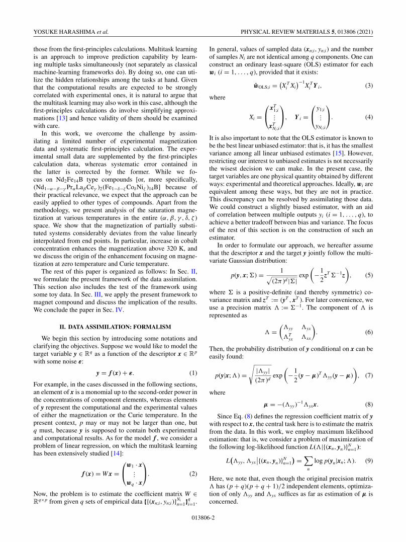
where x is an input parameter and the descriptor consists of(1, x, x2, x3). The data (i) and (ii) mimic computational andexperimental data, respectively. 10 samples for model (i) and 5for model (ii) were sampled randomly. Noise was applied withwidths 0.03 for yi and 0.1 for yii, respectively. An examplesample data and a result of the assimilation are shown inFig. 1. Although the sampled values of descriptors do notmatch between the two models, the prediction well agree withthe true model. We also compared with a simple least-squarefitting for these models separately. For the model (i), the OLSfit agrees with the true model as well as the assimilation.For the model (ii), however, the OLS fit disagrees with thetrue model for 0.5 < x < 1.0, whereas, the assimilation wellpredicts the true model even for that region.

The remaining issue is to determine the list of candidatesfor descriptors. Since, as we will see in Sec. III, the behaviorof the quantities of interest (e.g., magnetization, Curie tem-perature) is rather simple and we do not expect to encountera singular point where these quantities diverge, it suffices tomodel them by polynomial functions of the concentrationof each element. More specifically, we modeled the first-principles results by a second-order polynomial function:

ycomp =∑

iα+iβ+iγ +iδ+iζ�2

ciα iβ iγ iδ iζ αiαβ iβ γ iγ δiδ ζ iζ , (20)

where α, β, γ , δ, and ζ denote, respectively, the concentrationof Pr, La, Ce, Co, and Ni. As for the list of candidates forrelevant descriptors for R in Eq. (10), we considered a constantterm for the magnetization, and constant and δ linear terms forthe Curie temperature.

013806-3

YOSUKE HARASHIMA et al. PHYSICAL REVIEW MATERIALS 5, 013806 (2021)

FIG. 1. An example for the data assimilation. The true modelsare given by hand as (i) (blue solid curve) and (ii) (violet solid curve).Sample data generated from the true models are shown as bluesquares and violet points. The prediction from the data assimilationis shown as red for the model (i) and cyan for the model (ii). Theprediction from the OLS fit is also shown as a dotted-dashed line forcomparison.

III. MAGNETIZATION OF (Nd,Pr,La,Ce)2(Fe,Co,Ni)14B

A. Data assimilation for magnetization

Now that we have introduced a general procedure for thedata assimilation, the next step is to apply the methodologyto build up a flexible framework for predictions of the essen-tial properties of the magnetic compounds. By “flexibility”we mean the ability to predict the properties at an arbitrarytemperature, in addition to one for arbitrary combination ofthe doping concentrations.

A problem here is that both the experiments and first-principles calculations suffer from their limitations. On onehand, experiments are hard to perform at an arbitrary con-dition due to, e.g., difficulty in synthesis and limitation inexperimental facilities. On the other hand, density func-tional theory (DFT) [22,23], on which our first-principlescalculation are based, rely on an approximation to theexchange-correlation functional in practical applications. Fur-thermore, DFT only address the ground-state property of thesystem (in other words, the system at 0 K). Finite-temperaturemagnetism such as Curie temperature can be evaluated bycombining DFT with a mean field theory of classical spindynamics [24,25]. However, quantitative agreement with ex-periments is limited. Magnetism is a consequence of quantummany-body effect, which requires sophisticated theoreticaltreatment. Therefore, the experiments and the calculations arein a sense complementary to each other.

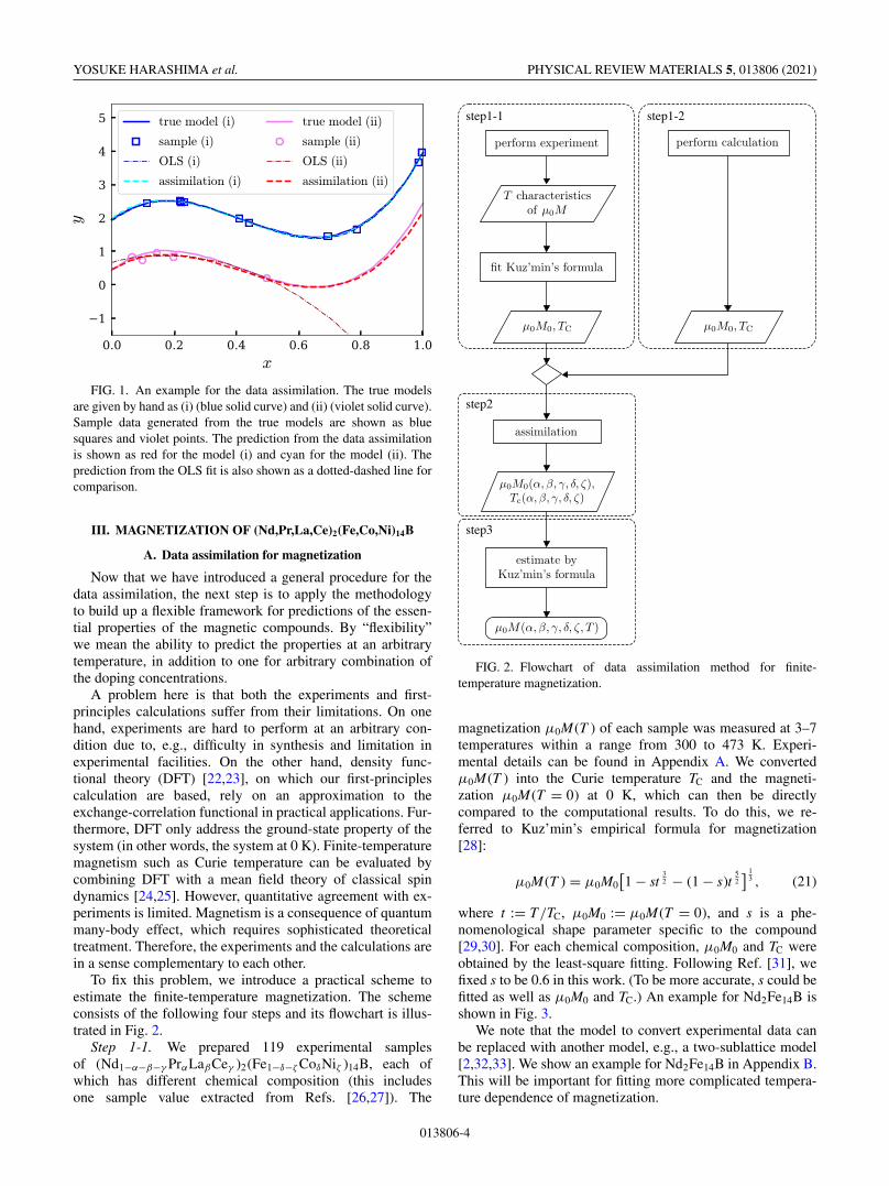
To fix this problem, we introduce a practical scheme toestimate the finite-temperature magnetization. The schemeconsists of the following four steps and its flowchart is illus-trated in Fig. 2.

Step 1-1. We prepared 119 experimental samplesof (Nd1−α−β−γ PrαLaβCeγ )2(Fe1−δ−ζ CoδNiζ )14B, each ofwhich has different chemical composition (this includesone sample value extracted from Refs. [26,27]). The

FIG. 2. Flowchart of data assimilation method for finite-temperature magnetization.

magnetization μ0M(T ) of each sample was measured at 3–7temperatures within a range from 300 to 473 K. Experi-mental details can be found in Appendix A. We convertedμ0M(T ) into the Curie temperature TC and the magneti-zation μ0M(T = 0) at 0 K, which can then be directlycompared to the computational results. To do this, we re-ferred to Kuz’min’s empirical formula for magnetization[28]:

μ0M(T ) = μ0M0[1 − st

32 − (1 − s)t

52] 1

3 , (21)

where t := T/TC, μ0M0 := μ0M(T = 0), and s is a phe-nomenological shape parameter specific to the compound[29,30]. For each chemical composition, μ0M0 and TC wereobtained by the least-square fitting. Following Ref. [31], wefixed s to be 0.6 in this work. (To be more accurate, s could befitted as well as μ0M0 and TC.) An example for Nd2Fe14B isshown in Fig. 3.

We note that the model to convert experimental data canbe replaced with another model, e.g., a two-sublattice model[2,32,33]. We show an example for Nd2Fe14B in Appendix B.This will be important for fitting more complicated tempera-ture dependence of magnetization.

013806-4

DATA ASSIMILATION METHOD FOR EXPERIMENTAL AND … PHYSICAL REVIEW MATERIALS 5, 013806 (2021)

FIG. 3. The magnetization of Nd2Fe14B as a function of temper-ature. The violet points denote the experimental observation. The reddashed curve is a regression curve derived from a least-square fittingto Eq. (21). The obtained values for μ0M(T = 0 K) and TC are alsoshown.

Step 1-2. On the theoretical side, we calculated the μ0M0

and TC following the method explained in Appendices C andD. The calculations were performed for 2869 compositionsuniformly distributed in the (α, β, γ , δ, ζ ) space.

Step 2. We then applied the data assimilation method tothe obtained μ0M0 and TC. We adopted the following regres-sion models:

μ0Mcomp0 (α, β, γ , δ, ζ ) =

∑I

McompI αiαβ iβ γ iγ δiδ ζ iζ , (22)

T compC (α, β, γ , δ, ζ ) =

∑I

T compI αiαβ iβ γ iγ δiδ ζ iζ , (23)

where I := (iα, iβ, iγ , iδ, iζ ). Both quantities were expandedup to the quadratic terms, namely 0 � ∑

j i j � 2. We as-sumed that the experimental data are correlated with thecomputational data as follows:

μ0Mexpt0 (α, β, γ , δ, ζ ) = Cmμ0Mcomp

0 (α, β, γ , δ, ζ ) + m0,

(24)

T exptC (α, β, γ , δ, ζ ) = Ct T

compC (α, β, γ , δ, ζ ) + t0 + t1δ.

(25)

The coefficients {McompI }I , Cm, m0 and {T comp

I }I , Ct , t0, t1 weredetermined by optimizing the likelihood (14) in terms of theparameters of the multivariate normal distribution yy andyx. Then, the coefficients were given by −(yy)−1yx asmentioned at Eq. (8).

In general, we may include higher-order terms to make aprediction model more flexible and accurate, which bringscomplexity in the determination of the coefficients in theprediction model. In the present case, we included the linearterm of δ in Eq. (25) and we will discuss that point later.

Step 3. The above data assimilation gives model functionsfor μ0M0 = μ0Mexpt

0 and TC = T exptC at arbitrary composition.

Applying Kuz’min’s formula (21) to these data, we estimateμ0M at finite temperature. In this way, we can predict the

experimental magnetization at arbitrary point in the (5 + 1)-dimensional space spanned by α, β, γ , δ, ζ , and T .

B. Results and discussion

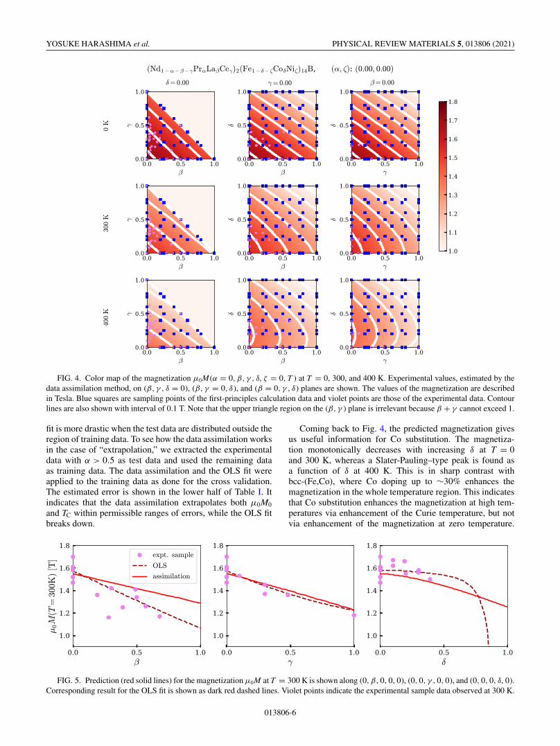
Figure 4 shows color maps of the magnetization on (β, γ ),(β, δ), (γ , δ) planes at 0, 300, and 400 K, where other vari-ables in α, β, γ , δ, ζ are set to zero in each case. We seethat the contour lines are not straight. This means that themagnetization varies nonlinearly in the composition space.The experimental data are unevenly distributed, which areinterpolated and extrapolated over the wide composition spacewith the help of computational data by the data assimilationmethod.

Figure 5 is a comparison of μ0M at T = 300 K betweenmeasured values and prediction by data assimilation and OLSfit along the β, γ , and δ axes. Estimated root-mean-squareerrors between the predictions and the experimental data at300 K are 0.085 T for the assimilation and 0.067 T for theOLS fit. It can be seen that both the predictions are able topredict the sampled experimental data, however, the OLS-fitmodel extremely decreases at the high-δ region where sam-ple points are absent. This seems to be typical behavior ofoverfitted models in which sampled data are well describedwhile prediction is sacrificed. On the other hand, the extremedecrease is not observed in the present assimilation method.The validity of prediction at the region can not be verifiedsince there are no experimental sample data there. Instead, wenext examine the generalizability of the predictions.

In order to examine the generalizability of the data assim-ilation method in comparison with the straightforward OLSfit, we performed 10-fold cross validation for the experimentalμ0M0 and TC. The experimental data were randomly dividedinto 10 groups. One of the groups was taken as test data andthe remaining were used for training. The data assimilationwas applied to the training data along with the whole com-putational data, then the root-mean-square error between thepredicted experimental value and the test data was evaluated.10 error values were obtained by changing test data to anothergroup. We iterated 10 sets of this procedure, and took anaverage of the errors. For the OLS fit, we used the trainingdata only (without computational data). As demonstrated inthe upper half of Table I, the average error of the presentmethodology was found to be significantly smaller than thatof the OLS fit, indicating high generalizability of the former.The advantage of the data assimilation compared to the OLS

TABLE I. Root-mean-square error for the assimilated predic-tions TC and μ0M0, corresponding to the components for theexperiment. The error for both the 10-fold cross validation (CV) andthe extrapolation are shown. In the extrapolation, the test data are theexperimental data in the range of α � 0.5. For comparison, results ofthe OLS fit are also shown.

OLS fit Data assimilation

10-fold CV TC (K) 172.5 43.8μ0M0 (T) 0.719 0.092

Extrapolation TC (K) 854.6 46.8μ0M0 (T) 6.180 0.097

013806-5

YOSUKE HARASHIMA et al. PHYSICAL REVIEW MATERIALS 5, 013806 (2021)

FIG. 4. Color map of the magnetization μ0M(α = 0, β, γ , δ, ζ = 0, T ) at T = 0, 300, and 400 K. Experimental values, estimated by thedata assimilation method, on (β, γ , δ = 0), (β, γ = 0, δ), and (β = 0, γ , δ) planes are shown. The values of the magnetization are describedin Tesla. Blue squares are sampling points of the first-principles calculation data and violet points are those of the experimental data. Contourlines are also shown with interval of 0.1 T. Note that the upper triangle region on the (β, γ ) plane is irrelevant because β + γ cannot exceed 1.

fit is more drastic when the test data are distributed outside theregion of training data. To see how the data assimilation worksin the case of “extrapolation,” we extracted the experimentaldata with α > 0.5 as test data and used the remaining dataas training data. The data assimilation and the OLS fit wereapplied to the training data as done for the cross validation.The estimated error is shown in the lower half of Table I. Itindicates that the data assimilation extrapolates both μ0M0

and TC within permissible ranges of errors, while the OLS fitbreaks down.

Coming back to Fig. 4, the predicted magnetization givesus useful information for Co substitution. The magnetiza-tion monotonically decreases with increasing δ at T = 0and 300 K, whereas a Slater-Pauling–type peak is found asa function of δ at 400 K. This is in sharp contrast withbcc-(Fe,Co), where Co doping up to ∼30% enhances themagnetization in the whole temperature region. This indicatesthat Co substitution enhances the magnetization at high tem-peratures via enhancement of the Curie temperature, but notvia enhancement of the magnetization at zero temperature.

FIG. 5. Prediction (red solid lines) for the magnetization μ0M at T = 300 K is shown along (0, β, 0, 0, 0), (0, 0, γ , 0, 0), and (0, 0, 0, δ, 0).Corresponding result for the OLS fit is shown as dark red dashed lines. Violet points indicate the experimental sample data observed at 300 K.

013806-6

DATA ASSIMILATION METHOD FOR EXPERIMENTAL AND … PHYSICAL REVIEW MATERIALS 5, 013806 (2021)

FIG. 6. Co concentration dependence of the Curie temperature ofNd2(Fe1−δCoδ )14B. Blue squares denote the first-principles data andviolet points denote the experimental data.

In Sm(Fe, Co)12, such reduction of the magnetization at zerotemperature and enhancement of the Curie temperature by Codoping have been also observed in experiment [6].

This conclusion is based on the fact that the TC increaseswith the Co concentration. However, it contains a tricky prob-

lem in the first-principles calculation. Figure 6 shows theCo concentration dependence of TC obtained by the experi-ment (step 1-1 in Fig. 2) and by first-principles calculation(step 1-2). As seen in the figure, the calculated value decreasesas the concentration increases, i.e., the trend is opposite fromthat of experiment. This discrepancy originates from theoret-ical errors in the first-principles data, which are systematicerrors but not accidental ones. It is a hard task to reducethe errors by improving approximations contained in the-oretical methods. However, such systematic errors can becomplemented by the data assimilation if there is a correla-tion between computational data and experimental data, eventhough the correlation is negative. In our scheme, the negativecorrelation in TC is expressed by the linear term in the rightside of Eq. (25).

Figures 7(a) and 7(b) show scatter plots of the magneti-zation at 300 and 400 K, respectively, where the predictedmagnetizations on uniform mesh points are plotted againstthe sum of Nd and Pr concentration (1 − β − γ ), which canbe regarded as the ratio of critical rare earths in the presentsystem. The dotted straight line connects the magnetizationsof two systems: La2Fe14B and Nd2Fe14B. While all the pointsare below the dotted line at 300 K, some points appear abovethe line at 400 K. This is attributed to the enhancementof the magnetization at high temperatures by Co doping.The maximum magnetization at T = 400 K is achieved in

FIG. 7. Scatter plots of the magnetization at (a) 300 K and (b) 400 K as a function of Nd and Pr concentration (1 − β − γ ). Thedotted straight line connects the magnetizations of two systems: La2Fe14B and Nd2Fe14B. (c) Cobalt concentration associated with chemicalcomposition giving maximum magnetization. The horizontal axis is temperature in Kelvin. The inset is an example of the magnetization at400 K of Nd2(Fe1−δCoδ )14B. A green point denotes the δmax at the temperature. (d) Magnetization at 400 K as a function of γ /(β + γ ). Othervariables are fixed in each line and sampled within the range of 0.0 � α � 0.2, 0.8 � β + γ � 1.0, 0.0 � δ � 0.3, and 0.0 � ζ � 0.1.

013806-7

YOSUKE HARASHIMA et al. PHYSICAL REVIEW MATERIALS 5, 013806 (2021)

Nd2(Fe, Co)14B with the cobalt concentration δmax = 0.18.Figure 7(c) shows the temperature dependence of δmax. Theδmax is nonzero above 320 K, and increases with raisingthe temperature. Finally, we analyze the magnetization as afunction of Ce concentration. In Fig. 7(d), the magnetiza-tion is plotted as a function of γ /(β + γ ) for fixed valuesof other variables α, β + γ , δ, ζ . Each line shows the resultfor different (α, β + γ , δ, ζ ). The magnetization is a convexupward function, and decreases with increasing the ceriumconcentration. This indicates that there is an optimum ceriumconcentration to effectively utilize abundant Ce element.

IV. CONCLUSION

We have proposed a data assimilation method in which asmall number of accurate data and a large number of lessaccurate data are integrated. The method enables us to pre-dict the behavior in the region where the former data arenot available. Based on this method, we have developed apractical scheme to estimate the finite-temperature magneti-zation at arbitrary composition. We applied the scheme to(Nd1−α−β−γ PrαLaβCeγ )2(Fe1−δ−ζ CoδNiζ )14B and obtainedthe magnetization in the five-dimensional composition space.Co addition enhances the magnetization above 320 K. It isnoticed that this is solely due to the fact that the Curie temper-ature rises by the Co addition: the magnitude of magnetizationat zero temperature cannot be enhanced.

ACKNOWLEDGMENTS

This work was supported by MEXT as “Programfor Promoting Researches on the Supercomputer Fugaku”(DPMSD). Part of the computation in this work was per-formed using the facilities of the Supercomputer Center of theInstitute for Solid State Physics at the University of Tokyo,and computational resources of the HPCI system through theHPCI System Research Project (Project No. ID:hp200125).

APPENDIX A: EXPERIMENTAL PROCEDURE

119 kinds of (Nd, Ce, La, Pr)13.55-(Fe, Co, Ni)80.54-B5.91

(at.%) alloys were prepared by arc melting. These alloyswere annealed at 1373 K for 24 h in Ar atmosphere. Thesealloys were pulverized and sorted into particles with diametersof <20 μm in an inert atmosphere to make magneticallyanisotropic powder. The powder density was determined usinga pycnometer (Ulrtapyc1200e, Quantachrome Instruments,USA). The powder compositions were measured by ICP-AES (ICPS8100, Shimazu, Japan) and the main phase, 2-14-1phase, ratio was calculated from the obtained composition.The magnetic physical properties were measured by using aVibrating Sample Magnetometer (VSM) (PPMS EverCool II,QuantumDesign, USA) at a maximum applied field of 9 T.

The powder was mixed with an epoxy resin in a Cu con-tainer and solidified in a magnetic field of 1 T to measure withVSM. The Magnetic Hysteresis (MH) curve of magneticallyeasy and hard direction was measured in the temperaturerange of 300 to 453 K. The anisotropy field (HA) was de-tected by singular point detection (SPD) method [34] fromMH curve of hard direction. When the anisotropy field is

less than 9 T, less than the applied magnetic field of VSM,HA can be detected by SPD. If the anisotropy field is over9 T, the MH curves for both of easy and hard direction wereextrapolated in high magnetic field to obtain the intersectionpoint, and the magnetic field at the intersection was made intoHA. On the other hand, the saturation magnetization (Js) wasestimated by the law of approach to saturation (LAS) [35–37]from the MH curve of easy direction. When HA was higherthan 9 T, which is the maximum applied field, Eq. (A1) wasused, and when it was sufficiently lower than 9 T, Eqs. (A2)and (A3) were used. Js is saturation magnetization and b andχ0 are constants. The χ0H term is often referred to as theso-called paramagnetismlike term [38]. Equations (A2) and(A3) dealing with the χ0 term is more accurate for measuringsaturation magnetization, but there is a condition that the ap-plied magnetic field is sufficiently larger than the anisotropicmagnetic field. The saturation magnetization estimated by theLAS was divided by the main phase ratio of powder to obtainthe saturation magnetization of the 2-14-1 phase in thesecompositions, where the grain boundary phases other than themain phase were treated as paramagnetic phases:

J = Js

(1 − b

H2

), (A1)

J = Js

(1 − b

H2

)+ χ0H, (A2)

dJ

dH= Js

(2b

H3

)+ χ0. (A3)

APPENDIX B: AN EXAMPLE OFTWO-SUBLATTICE MODEL

The scheme for finite-temperature magnetization shownby the flowchart of Fig. 2 includes the steps for modelingtemperature dependence of magnetization. In this study, weuse Kuz’min’s formula for the modeling. A two-sublatticemodel [2,32,33] is one of the other possible models to replacethe steps. Then we demonstrate the fitting by using the two-sublattice model for Nd2Fe14B, which corresponds to Fig. 3in the case of Kuz’min’s formula.

The two-sublattice model is defined as

μR(T ) = μR0BJ(μBμR0HR(μR, μT )/kBT

), (B1)

μT (T ) = μT 0BS(μBμT 0HT (μR, μT )/kBT

), (B2)

where the subscripts R and T denote rare-earth and transitionmetal elements. BJ is the Brillouin function defined as

BJ (x) ≡ 2J + 1

2Jcoth

(2J + 1

2Jx

)− 1

2Jcoth

(1

2Jx

), (B3)

and molecular fields for rare-earth and transition metal atomsare

HR(μR, μT ) = d (2nRRμR + 14nRT μT ), (B4)

HT (μR, μT ) = d (2nRT μR + 14nT T μT ). (B5)

μR and μT are the local magnetic moments of rare-earth andtransition metal atoms. μR0 and μT 0 are the correspondingvalues at zero temperature, and we here fix μR0 as 3.3 μB

013806-8

DATA ASSIMILATION METHOD FOR EXPERIMENTAL AND … PHYSICAL REVIEW MATERIALS 5, 013806 (2021)

FIG. 8. The magnetization of Nd2Fe14B predicted by using thetwo-sublattice model, Eqs. (B1) and (B2).

for Nd. J and S are the free-ion moments of rare-earth andtransition metal atoms, and thus, J = 9

2 and S = 1. μB is theBohr magneton. d ≡ μ0μB/V is a constant to convert theunit of magnetic moment (Bohr magneton) to that of mag-netization (Tesla). μ0 is the vacuum permeability and V isa volume of Nd2Fe14B per formula unit. nRR, nT T , and nRT

are the dimensionless molecular-field coefficients which rep-resent magnetic couplings of R-R, T -T , and R-T , respectively.The magnetization is given as

μ0M(T ) = d[2μR(T ) + 14μT (T )]. (B6)

To obtain μR and μT at a temperature, we solve the simul-taneous Eqs. (B1), (B2), (B4), and (B5) self-consistently. Weoptimize μT 0, nRR, nT T , and nRT such that the experimentaldata are well predicted. The result is shown in Fig. 8. In thepresent case, there is no qualitative difference from Kuz’min’sformula of Fig. 3. When the temperature dependence willbe more complicated, such as ferrimagnetism, this will beimportant.

APPENDIX C: FIRST-PRINCIPLES CALCULATION

We perform density functional theory calculationfollowing Korringa-Kohn-Rostoker (KKR) [39,40] Green’sfunction approach in the atomic sphere approximation(ASA) incorporating coherent potential approximation(CPA) [41,42] as implemented in AKAIKKR [43].Continuous interpolation over 0 � α, β, γ , δ, ζ � 1 for(Nd1−α−β−γ PrαLaβCeγ )2(Fe1−δ−ζ CoδNiζ )14B is done on thebasis of KKR-CPA. The local spin density approximationas parametrized by Moruzzi, Janak, and Williams [44] isadopted for the exchange-correlation energy functional. Weset lmax = 2 putting all 4 f electrons of the valence stateon the basis of open-core approximation. We assume eachconfiguration of the electrons as Nd3+, Pr3+, and Ce4+,respectively. Contributions from 4 f electrons of Nd and Pr tothe magnetic moments are restored manually.

Intersite magnetic exchange couplings are calculated usingthe method developed by Liechtenstein et al. [45]. The Curie

temperature is evaluated by solving the derived Heisenbergmodel in the mean field approximation.

APPENDIX D: LATTICE PARAMETERS

We collected experimental lattice parameters of R2T14B(R = Nd, La, Ce, Pr; T = Fe, Co, Ni) from literature [2][Table II(a)]. However, some of them are not available. Inorder to evaluate the lattice parameters for these missingpoints, we performed first-principles calculation based ondensity functional theory [22,23] in the generalized gradientapproximation with Perdew-Burke-Ernzerhof formula [46]using VASP code [47] [Table II(b)]. We integrated the calcu-lated lattice parameters a and c with the above experimentaldata assuming the following simple form:

acomp =∑

I

acompI αiαβ iβ γ iγ δiδ ζ iζ , (D1)

ccomp =∑

I

acompI αiαβ iβ γ iγ δiδ ζ iζ , (D2)

aexpt = Caacomp + a0, (D3)

cexpt = Ccccomp + c0, (D4)

where I := (iα, iβ, iγ , iδ, iζ ) runs under the condition0 � ∑

j i j � 1. Using the data assimilation methodexplained in Sec. II, we determined the coefficients{acomp

I }, {ccompI },Ca, a0,Cc, c0, from which aexpt and cexpt for

the missing points are estimated [Table II(c)]. We interpolatedlattice parameters for nonstoichiometric systems accordingto Vegard’s law by using the obtained lattice parameters forstoichiometric systems.

TABLE II. Lattice parameters (a, c) of R2T14B for R = Nd, La,Ce, Pr and T = Fe, Co, Ni. (a) Experimental values taken fromRef. [2], (b) computational results, and (c) values obtained by thedata assimilation technique to complement the unavailable valuesof (a).

(a) Fe Co Ni

Nd (8.80, 12.20) (8.64, 11.86)La (8.82, 12.34) (8.67, 12.01)Ce (8.76, 12.11)Pr (8.80, 12.23) (8.63, 11.86)

(b) Fe Co NiNd (8.73, 12.07) (8.58, 11.74) (8.57, 11.75)La (8.75, 12.16) (8.61, 11.80) (8.59, 11.79)Ce (8.70, 11.96) (8.55, 11.63) (8.54, 11.62)Pr (8.75, 12.11) (8.59, 11.77) (8.59, 11.77)

(c) Fe Co NiNd (8.62, 11.89)La (8.65, 11.93)Ce (8.61, 11.77) (8.60, 11.75)Pr (8.64, 11.91)

013806-9

YOSUKE HARASHIMA et al. PHYSICAL REVIEW MATERIALS 5, 013806 (2021)

[1] M. Sagawa, S. Fujimura, N. Togawa, H. Yamamoto, and Y.Matsuura, J. Appl. Phys. 55, 2083 (1984).

[2] J. F. Herbst, Rev. Mod. Phys. 63, 819 (1991).[3] T. Miyake and H. Akai, J. Phys. Soc. Jpn. 87, 041009 (2018).[4] F. Kools, A. Morel, R. Grössinger, J. L. Breton, and P. Tenaud,

J. Magn. Magn. Mater. 242–245, 1270 (2002).[5] A. K. Pathak, M. Khan, K. A. Gschneidner Jr., R. W. McCallum,

L. Zhou, K. Sun, K. W. Dennis, C. Zhou, F. E. Pinkerton, M. J.Kramer, and V. K. Pecharsky, Adv. Mater. 27, 2663 (2015).

[6] Y. Hirayama, Y. K. Takahashi, S. Hirosawa, and K. Hono,Scr. Mater. 138, 62 (2017).

[7] R. E. Bellman, Adaptive Control Processes: A Guided Tour(Princeton University Press, Princeton, 1961).

[8] A. Alam, M. Khan, R. W. McCallum, and D. D. Johnson,Appl. Phys. Lett. 102, 042402 (2013).

[9] P. Tenaud, A. Morel, F. Kools, J. Le Breton, and L. Lechevallier,J. Alloys Compd. 370, 331 (2004).

[10] W. Körner, G. Krugel, and C. Elsässer, Sci. Rep. 6, 24686(2016).

[11] P. Nieves, S. Arapan, J. Maudes-Raedo, R. Marticorena-Sánchez, N. Del Brío, A. Kovacs, C. Echevarria-Bonet, D.Salazar, J. Weischenberg, H. Zhang et al., Comput. Mater. Sci.168, 188 (2019).

[12] T. Fukazawa, Y. Harashima, Z. Hou, and T. Miyake, Phys. Rev.Mater. 3, 053807 (2019).

[13] N. Papanikolaou, R. Zeller, and P. H. Dederichs, J. Phys.:Condens. Matter 14, 2799 (2002).

[14] L. Breiman and J. H. Friedman, J. R. Stat. Soc.: Ser. B Stat.Methodol. 59, 3 (1997).

[15] T. Hastie, R. Tibshirani, and J. Friedman, in The Elements ofStatistical Learning: Data Mining, Inference, and Prediction(Springer, New York, 2009), pp. 43–99.

[16] C. Stein, in Proceedings of the Third Berkeley Symposium onMath Statistics and Probability (University of California Press,Berkeley, CA, 1956), Vol. 1, pp. 197–206.

[17] B. Efron and C. Morris, J. Am. Stat. Assoc. 70, 311 (1975).[18] D. B. Rubin, Biometrika 63, 581 (1976).[19] C. G. Broyden, IMA J. Appl. Math. 6, 76 (1970).[20] R. Fletcher, Comput. J. 13, 317 (1970).[21] R. H. Byrd, P. Lu, J. Nocedal, and C. Zhu, SIAM J. Sci. Comput.

16, 1190 (1995).

[22] P. Hohenberg and W. Kohn, Phys. Rev. 136, B864 (1964).[23] W. Kohn and L. J. Sham, Phys. Rev. 140, A1133 (1965).[24] N. M. Rosengaard and B. Johansson, Phys. Rev. B 55, 14975

(1997).[25] M. Pajda, J. Kudrnovský, I. Turek, V. Drchal, and P. Bruno,

Phys. Rev. B 64, 174402 (2001).[26] S. Hock, Ph.D. thesis, Universität Stuttgart, 1988.[27] R. Grössinger, X. K. Sun, R. Eibler, K. H. J. Buschow, and

H. R. Kirchmayr, J. Phys. Colloques 46, C6-221 (1985).[28] M. D. Kuz’min, Phys. Rev. Lett. 94, 107204 (2005).[29] M. D. Kuz’min and A. M. Tishin, Phys. Lett. A 341, 240

(2005).[30] M. D. Kuz’min, M. Richter, and A. N. Yaresko, Phys. Rev. B

73, 100401(R) (2006).[31] M. Ito, M. Yano, N. M. Dempsey, and D. Givord, J. Magn.

Magn. Mater. 400, 379 (2016).[32] C. Fuerst, J. Herbst, and E. Alson, J. Magn. Magn. Mater.

54–57, 567 (1986).[33] R. Skomski, Simple Models of Magnetism (Oxford University

Press, Oxford, 2008).[34] R. Cabassi, Measurement 160, 107830 (2020).[35] N. S. Akulov, Z. Phys. 69, 822 (1931).[36] G. Hadjipanayis, D. J. Sellmyer, and B. Brandt, Phys. Rev. B

23, 3349 (1981).[37] H. Kronmüller and M. Fähnle, Micromagnetism and the Mi-

crostructure of Ferromagnetic Solids (Cambridge UniversityPress, Cambridge, 2003).

[38] H. Zhang, D. Zeng, and Z. Liu, J. Magn Magn. Mater. 322, 2375(2010).

[39] J. Korringa, Physica (Amsterdam) 13, 392 (1947).[40] W. Kohn and N. Rostoker, Phys. Rev. 94, 1111 (1954).[41] H. Shiba, Prog. Theor. Phys. 46, 77 (1971).[42] H. Akai, Phys. B+C (Amsterdam) 86-88, 539 (1977).[43] H. Akai, AKAIKKR, http://kkr.issp.u-tokyo.ac.jp/.[44] V. L. Moruzzi, J. F. Janak, and A. R. Williams, Calculated

Properties of Metals (Pergamon Press, New York, 1978).[45] A. Liechtenstein, M. Katsnelson, V. Antropov, and V. Gubanov,

J. Magn. Magn. Mater. 67, 65 (1987).[46] J. P. Perdew, K. Burke, and M. Ernzerhof, Phys. Rev. Lett. 77,

3865 (1996).[47] G. Kresse and D. Joubert, Phys. Rev. B 59, 1758 (1999).

013806-10