Physics 111A Final Project: ECG

Author: Derek Perera // Partner: William Liu

December 16, 2019

(a) Hardware (b) LabView Software(c) Right: Derek Perera (Author);Left: William Liu

Figure 1: Electrocardiogram Project

Figure 2: Grading Matrix

1

1 Introduction

For our final project, we chose to construct and analyze an electrocardiogram (ECG). ECGs are conceptuallysimple: the idea is to amplify the electrical potential created during a heartbeat. The result of a typical ECGis a graph of voltage per time, making it an application that can be directly observed on the oscilloscope.While the general idea of the ECG is fairly simple, in practice it is a difficult circuit to build largely due to twomain issues. The first is that the heartbeat produces a very small signal that is extremely variable dependingon the patient. According to [1], the amplitude of the heartbeat depends on the size of the patient’s heartand the placement of the electrodes on his or her chest1. For the purposes of our design, we assumed thehuman heartbeat to have an amplitude of approximately 3 mV2. The second main issue concerns noise. Thehuman body contains plenty of noise that makes it difficult to discern a signal from the heartbeat regardlessof its amplification. As a result, we needed to include an extensive amount of filtering in both our circuitand subsequent LabView programs3. In this project, we were able to overcome these two issues by using aninstrumentation amplifier and a Sallen-Key bandpass filter. In addition, source followers were added betweeneach component. Figure 3 details our full block diagram for this project.

Figure 3: ECG Block diagram

There ended up being only three components of our final circuit: an Instrumentation Amplifier, Sallen-Key Bandpass filter, and a speaker circuit section consisting of a hysteretic comparator, JFET switch, andInverting amplifier. Each of these components served a specific purpose in helping us get a strong signaloutput from our heartbeats. The instrumentation amplifier helped us amplify the potential difference createdby our heartbeat, measured by two electrodes placed on either side of the chest in order be as close as possibleto the heart. This type of amplifier is very similar to the differential amplifier studied in Lab 5 [5], withthe main difference of utilizing op-amps for amplification rather than JFETs. The reason for us using thistype of amplifier is that the differential amplifier, while doing the same thing, is highly dependent on howwell-matched the two JFETs are. Considering that our input signal was expected to be a very noisy andvery low amplitude and frequency signal, we did not want to deal with the complications and errors thatwould further be caused by imperfectly matched JFETs. Thankfully, the instrumentation amplifier’s use ofop-amps as its primary mode of amplification alleviates this issue This circuit component can be describedby the following equation4:

1A full description of the specific anatomy and cardiology necessary for this project is given in the ’Theory’ Section.2This is a very rough estimate. We intentionally chose a very weak heartbeat amplitude in order to ensure that our amplifier

would correctly amplify any signal regardless of strength. This 3 mV estimate was used as our input signal to test eachcomponent in our circuit.

3Further and more in depth descriptions of filtering used in the project are included in the following section.4This equation is properly analyzed in Section 2.

1

Vout = (V2 − V1)(1 +2R

RG) (1)

It is important to note that our use of this specific type of amplifier is key as it amplifies the differencebetween two voltage inputs, rather than one signal input like most simple amplifiers such as the invertingand non-inverting amplifiers. Additionally, The Sallen-Key Bandpass filter is constructed using a low passSallen-Key filter, followed by a source follower and a high pass Sallen-Key filter. Our use of a Sallen-Keyfilter in our circuit as opposed to a standard 2-pole RC filter is that this filter is more sharply attenuatedaround its 3 dB point, while the RC filter tends to asymptote less sharply. This sharpness allows for morecontrol in our filtering and for more defined passbands. It is important to note that Chebyshev filters (suchas the Sallen-Key topology filters constructed in Lab 7 [5]) do experience ripples as a result of abrupt signalchanges, hence why we did not choose to use Chebyshev filters instead favoring the simpler Sallen-Key filters5.Sallen-Key filters, both low and high pass, follows the following equation [5] for the frequency boundary:

f =1

2π√R1R2C1C2

(2)

Furthermore, the speaker circuit is a fairly simple circuit using two basic circuit components extensivelystudied in this class: the hysteretic comparator and the JFET switch. The hysteretic comparator outputseither positive or negative 12 V depending on whether its input is positive or negative, a phenomena controlledby the magnitude of the potentiometer [5]. Notably, it obeys the voltage divider equation:

ξ =R1

R1 +R2(3)

The JFET switch [5] is controlled by a 500 mV, 1 kHz square wave signal to its gate, and this input willbe switched off when the output signal from the hysteretic comparator is positive, and since the only timesthat this will be positive is when the heart beats to its peak, the speaker will output a constant sound exceptat these heartbeats, thus making it possible to hear the heartbeat.

Lastly, our circuit utilizes some other minor circuit components included to improve the performance.These include both the non-inverting and inverting amplifiers. These two circuits obey equations 4 and 5respectively [5].

VoutVin

=R2

R1+ 1 (4)

VoutVin

= −R2

R1(5)

A full analysis of our entire ECG circuit and accompanying programs is given in the following section.

2 Circuitry and Programming

Figure 4 shows our full ECG circuit diagram. Since our circuit is quite large, the diagram is drawn goingdown the page, leading to a convenient split of the diagram into three sections: Amplification, Filtering, andSpeaker setup. Starting with the instrumentation amplifier (shown in Figure 5) in the first section, we choseto use this type of amplifier instead of the JFET based differential amplifier as we wanted to eliminate thedifficulties associated with JFET matching in the differential amplifiers, as stated before. It is importantto note the inclusion of two 510 kΩ resistors immediately before each of the inputs are fed into the positiveinput of the first two op-amps. These resistors are included for safety reasons. Since we are using LF356Nop-amps for this ECG, there is a lot of current flowing throughout our circuit due to this type of op-amprequiring a 12V power supply to function. Thus, since we are using direct contact with our body at the heartregion as our input, we use fairly large resistors for protection at the beginning in case of any current thatmay flow back to us for whatever reason.

5In hindsight, since the heartbeat signal can be simplified as a sharp and brief perturbation in an otherwise constant signalit would be reasonable to neglect this effect as it should not have a significant effect on our output. Nevertheless, our circuituses general Sallen-Key filters

2

Figure 4: ECG circuit diagram. All op-amps are decoupled using 0.1 µF capacitors.

Figure 5: Instrumentation amplifier circuit diagram

3

The instrumentation amplifier follows Equation 1, with RG = 10 Ω, R = 1kΩ6, and V1 and V2 being theChest left and Chest right input respectively. This equation is obtained by considering the two leftmost op-amps (connected to the two chest inputs) as being a part of either a non-inverting or inverting amplifier. Thisis easy to see as if V2 is grounded, then the upper circuit is a non-inverting amplifier (obeying Equation 4)and if V1 is grounded, then the lower circuit will be an inverting amplifier7 (obeying Equation 5). Combiningthese two relationships, we get the following two relationships for V+ and V− (V+ is the immediate outputof the lower op-amp while V− is the immediate output of the upper op-amp):

V+ =R

RG(V2 − V1) + V2 (6)

V− =R

RG(V1 − V2) + V1 (7)

Since we set R = 1kΩ, the right-most op-amp has a gain of 1, so:

Vout = V+ − V− (8)

So plugging in Equations 6 and 7 into Equation 8 yields Equation 1. Using our values of R and RG, ourinstrumentation amplifier was designed to have a Gain of 201. We want our amplifier to have a high gaindue to the very small nature of the human heartbeat signal. We included a source follower immediately afterthe instrumentation amplifier in order to aid in debugging the circuit.

For the filtering section of the ECG, we utilized the Sallen-Key bandpass filter design. This diagramis located in the middle part of Figure 4. This filter is actually a lowpass and highpass Sallen-Key filterconnected in series. Mathematical analysis of these circuits is fairly involved, but thankfully since both thehigh and low pass Sallen-Key filters are symmetric (the circuits only differ by exchanging the placement ofthe resistors and capacitors), they yield the same solution as mentioned in Equation 2. This can be obtainedby analyzing the circuit using the op-amp golden rules and Kirchoff’s circuit loops. Importantly, the transferfunction for Sallen Key filters is (s = jω; Q is defined to be the Q factor which describes the damping ofspecific circuits):

H(s) =ω20

s2 + s(ω0

Q ) + ω20

(9)

In order to derive Equation 2, we must find the ratio of the output of the filter to the input of the filter,which is dependent on the the impedance of each component of the filter. Setting this equal to the transferfunction will allow us to solve for ω0.

As an example, the low pass Sallen key filter can be solved via circuit analysis, yielding the following twoequations (V1 is the voltage at the point immediately after the first resistor R1):

Vin − V1R1

= jwC2Vout −Vout − V1

1jwC1

(10)

V1 = Vout(R2jwC2 + 1) (11)

Plugging Equation 11 in to Equation 10, solving for the ratio of output to input voltage, then equating theresult to the transfer function will yield8:

ω0 =1√

R1R2C1C2

(12)

This is an identical form to Equation 2. Doing this entire process again for the high pass filter requires usto swap the impedance positions of R1 with C1 and R2 with C2. Solving again will yield the same result,

6The gain of the instrumentation amplifier heavily depends on how well matched the R resistors are. However, in testingthis circuit, we found very little difference between using normal 1kΩ resistors and 1% 1kΩ resistors. While our final circuituses 1% 1kΩ resistors, we did not include that note in our diagram because it did not in fact have an effect on our amplifier’sperformance.

7Since the upper op-amp is a non-inverting amplifier, the input must be positive if we are to see the QRS complex as apositive spike (see Section 3).

8This step is admittedly a bit confusing. There is a bit of algebra involved but the general idea is that by finding the ratioof the output over input voltage and equating to equation 9, the form of the transfer function results. Thus equating thenumerators is all that is now necessary to get equation 12.

4

which is reasonable to infer given the symmetry between the low pass and high pass filters. There is a sourcefollower placed in between these two filters in order to once again assist in debugging this part of the circuit.Using the values mentioned in Figure 4, we achieve a bandpass from 0.403 Hz to 159 Hz. We designed thisbandpass filter to have a narrow bandpass because the human body produces plenty of noise especially athigh frequencies. Having the boundary at 159 Hz allows this high frequency noise to be attenuated away.It is also important to note that the gain of the Sallen-Key filter is very small since we are using relativelylarge resistors and a very small input voltage. Thus, we neglect the filter’s gain for analysis.

The speaker circuit (located in the bottom part of Figure 4) consists of a hysteretic comparator and aJFET switch. Importantly, a non-inverting amplifier is added just before this circuit with a gain of 11. Thisis to make sure that the incoming heartbeat signal is in fact large enough to both turn on the LED andspeaker. The hysteretic comparator follows the voltage divider relationship as described (Equation 3) in Lab6 [5]. Our design allows the heartbeat to function as the input signal. The potentiometer voltage controlsthe output of this circuit, with the output being either positive or negative 12V depending on when thepotentiometer voltage passes the input heartbeat. In our circuit, we assumed that the signal between theheartbeat peaks would be zero, so that at every heartbeat, the comparator would output +12V while at allother points the circuit would output -12V. The JFET switch controls the speaker. There is a 100 kΩ resistorimmediately before the JFET in order to ensure that the JFET does not burn out. Our output from thehysteretic comparator is inputted into the gate of the transistor. Since the gate is forward biased, it will onlyturn on when this signal is positive, which is at the peak of each heartbeat. We also pass a 500 mV 1 kHzsignal through the drain. This signal will be amplified by a gain of 10 by an inverting amplfier immediatelyafter the switch before powering the speaker. Since the JFET switch is controlled by the heartbeat, wedesigned the speaker to beep in tune with our heartbeats since the switch will only pass the positive peaks ofthe heartbeat. In addition, an offshoot of this part of the circuit includes an LED. This part is very simpleas it only contains a resistor to prevent burnout and the LED, which will light up at positive peaks as wellsince it is in parallel.

Lastly, we used LabView to program a BPM calculator and R wave amplitude measurement. The methodsfor this program are straightforward. Immediately after the bandpass filter, we feed the heartbeat into theDAQ. The reason for using the signal after the bandpass is because this point has the least amplified andleast noisy signal in the circuit, making it easier to measure the amplitude9. The program first attains theheartbeat signal using the DAQ assistant. It is then filtered using the filtering VI, with the filter being set asa Butterworth filter to third order. We use a Butterworth filter as it is the default setting and also happensto produce the most clean signal. This filtered signal is fed into the waveform generator. Simultaneously, allthis signal processing is done in a for loop that sets the number of 10 second samples10. The filtered signalis also processed using a built-in VI that locates the maximum R wave amplitudes of the input signal alongwith the S wave valley locations in the sample, taken to represent the timing of the heartbeat. This allowsus to get the time period between beats and the maximum amplitude of each heartbeat in the sample. Afterthis, the R wave amplitude is taken to be the average amplitude of the sample and the BPM is calculated byconverting the period between beats into a frequency and averaging this value to get the average heartbeatfrequency. Multiplying this by 60 gets us the BPM. Analysis of the functionality of this LabView programis given in the Results section.

3 Theory

There is a considerable amount of theory associated with this project, mostly in the practice of electrocar-diography. Figure 6 shows the QRS complex, or the heartbeat. When feeding the output of our ECG intothe oscilloscope or into the DAQ, the primary signal that we will see is this complex. Just by looking atit, it is obvious to tell that the R amplitude is significantly larger than the Q and S. Due to its prominentstructure, the R wave peak is where the amplitude of the heartbeat was measured, thus we will distinguishit by calling it the R wave amplitude. The cardiology of the heartbeat involves the atria contracting andmoving blood into the ventricles (R wave), followed by the ventricles contracting with the atria relaxing andblood simultaneously flowing out of the heart. This entire process lasts ∼0.08 seconds [1]. However, we aremore concerned with the electrical pulses generated by the heartbeat. The electrical signals in the heart

9The calculation for the approximate amplitude of our heartbeat was corrected for the gain of the instrumentation amplifierby hand.

10In order to get a more accurate BPM and amplitude, our program samples 10000 times over 10 seconds, with the expectationthat approximately 10 heartbeats will measured.

5

Figure 6: QRS Complex, commonly known in conversation as the ’heartbeat’.

control both the heart rate and rhythm [2]. The cells in the heart that are designed to do this are known asthe Bundle of His cells. These cells transmit electrical signals to the ventricles, allowing them to contract.Thus, the Bundle of His cells are the heart’s mechanism for producing its main voltage pulse11[3]. Replicationof the R wave as a positive voltage signal spike has to do with the the placement of the electrodes. Sincethe electrical transmission of the heart’s electric signals flows from the atria to the ventricles12, and since theheart is tilted to the left, this means that that the pulse flows from the Chest right electrode to the Chestleft electrode. This requires that the Chest Left electrode be inputted into the upper op-amp (V1) of theinstrumentation amplifier since that op-amp is a non-inverting amplifier. This allows the total output to bepositive for the R wave since the positive input is not inverted by the amplifier. The Chest right electrodemust therefore be in the V2 position, thus ensuring positive Vout. Admittedly, there is a practical amountof error in our ECG since there is a strong likelihood that our electrodes are placed incorrectly, simply dueto the fact that we are not doctors and are not professionally trained in finding where the optimal electrodelocations.

In addition, when studying the functionality of our BPM, we used the classic two finger test in orderto get an estimate of our heart rates. This involves counting the number of measured heartbeats13 over 15seconds and multiplying by 4 to get a BPM. Due to the impracticality of this method as being an accurateheart rate measurement, we assign a good amount of error to values measured in this method. Nevertheless,given our limited materials this was the easiest and quickest way to check the efficiency of our BPM program.

4 Experimental Procedure

Given that we had a healthy amount of freedom to explore the functionality of our ECG, our experimentincluded multiple small parts in order to test for functionality. Our first test for functionality involvedattempting to get an LED to light up in tune with our heartbeats14. This process was tested at first usingtwo test inputs of 20 mV and 3 mV15 1 Hz pulses generated from the signal generator, serving as our ideal,artificial, test heartbeats. Since the signal generator can generate consistent and clean signals, they provedto be an ideal version of our actual heartbeats, and thus very useful in testing and debugging our initialcircuit. Each component (except the DAQ) was first tested using these two signals. For the LED, we createdan offshoot of our general circuit right after the non-inverting amplifier where we placed the LED, as visiblein Figure 4. After testing the LED and its ability to flicker on and off with our test inputs, we then used ourown heartbeats. The second test was the test of the speaker, conducted in the same way as the LED. Lastly,

11The transmission of the electrical signals by the Bundle of His cells is thought to be the cause of the P-R interval, or thepart of the heartbeat just before the QRS complex [3]. The P wave is generally too small and swamped with noise for us todiscern using our ECG.

12Biologically, this is known as ventricular depolarization [4].13Typically this is done by placing two fingers on the wrist. However, I personally found it difficult to locate my pulse here,

so I measured by placing two fingers on my neck.14Technically, our first test was attempting to get our heartbeats to be discernible on the oscilloscope. However, this was done

alongside every test during the duration of our experiment, so it merely served as an indicator that our electrodes were pickingup our heartbeats.

15This 3 mV signal was created using a non-inverting amplifier with a gain of 0.15. We fed the 20 mV directly to the inputas well as this non-inverter in order to get the 3 mV signal.

6

we tested our ECG using the DAQ and a LabView program written to take our heartbeat as an input andcalculate the QRS amplitude and heart rate in BPM. This test was not conducted using the low voltage testinputs, as by this point, we had already confirmed the functionality of our circuitry. It is also important tonote that the input signal fed into the DAQ and our program were from the output of the bandpass filter.This is because there is extra amplification in the speaker part of our circuit, so using the output directlyfrom the filters only requires us to correct for the gain of the instrumentation amplifier. This last test was alsothe only test that we could evaluate quantitatively. The following section contains an extensive discussion ofthe results of our experiments.

5 Results and Discussion

For this results discussion, we consider the LED and speaker as one system and the DAQ as the other.The reasons for this are that the LED and speaker essentially depend on the same signal, so it will serveas an analog circuit analysis while the DAQ will be treated as an analysis of the efficiency of our LabViewalgorithm.

Starting with our ECG circuit, our main issue ended up being the acquisition of the heartbeat usingelectrodes. We attempted this in two ways: using a dime and a penny16 as makeshift electrodes and usingactual medical electrodes. It turned out that dime and penny were not that bad at acquiring the heartbeatsignal. It took some time to figure out where on the chest was best to place them, causing us to initiallyhave difficulty getting a signal. One advantage of using the coins was that it was easy to move them aroundour chests until we found a location where the signal could be seen (this was not as simple with the medicalelectrodes since they are designed to stick to one spot). The medical electrodes were definitely designed tobe better at acquisition, however soldering wires to them proved to be difficult due to the irregular shapeof the conductive surface. In terms of functionality, while both electrodes proved to be difficult in actuallyseeing the heartbeat on the oscilloscope, both were able to attain a good heartbeat signal. With enoughpractice, we were eventually able to recover our heartbeat signal with either electrode fairly quickly. It is alsoworth mentioning that, near the end of this project, we simply strategically taped wires onto the electrodesin order to save time. This did not effect the acquisition or quality of our attained heartbeat. An image ofour acquired heartbeat is shown in Figure 7.

Getting the LED to light up ended up being easier than getting a sound on the speaker, although bothwere achieved with success. For the LED, we managed to get the light to flicker at the tune of our heartbeat,with the luminosity of the light dependent on how well the signal was getting acquired by the electrodes andhow positive or negative the baseline was for our signal. This latter problem turned out to be the only majorproblem in functionality. Due to the imperfectness of our electrodes, our electrodes would occasionally losethe signal sporadically. Once reacquired (usually after slight adjustment) the signal would slowly asymptoteback to the baseline. This baseline in theory should always be at 0V; however, in practice we observedthe baseline to sometimes be slightly above or below 0V, resulting in the LED either being always lit andbrightening at the heartbeat peaks (above 0V) or being always off and only barely lighting up (below 0V).Regardless, there was always an indication of the heartbeat flickering the LED, with only the extent beingeffected by this imperfect baseline.

Similarly, the speaker witnessed the same issue, just in the form of an audio output. Depending on thebaseline, the audio would either always remain off and turn on when the heartbeat peaks (below 0V andwhat we expect) or always remain on and turn off during the S wave peak as it dipped below zero. Due tolingering noise in the signal, the latter was a far more common observance due to the noise causing the signalto perpetually be positive except at the S wave. Despite this, there once again was always an indication ofthe heartbeat due to speaker reacting at each peak.

One slight alleviation to this issue was by grounding the Chest Left input to our bodies. This is commonin medical ECGs and we achieved it by connecting an electrode attached to our legs in series with a 10 MΩresistor to the Chest Left input. What we observed did not completely solve the problem in that the baselineremained slightly offset from 0V; however, this self-grounding technique made it quicker to reacquire theheartbeat signal if ever lost and more consistently return the baseline on the scope to a value close to 0V.So, while not a full solution to the problem, self-grounding did alleviate this issue.

16Since dimes and pennies are mostly copper, we figured that they could be effective conductors and thus be used as quickelectrodes. They were constructed by soldering a wire to each coin and placing the coins directly to the chest, making sure tocontact the coin and skin as much as possible to maximize surface area and hold them against our chest using our shirts (usinga finger would ground the electrode).

7

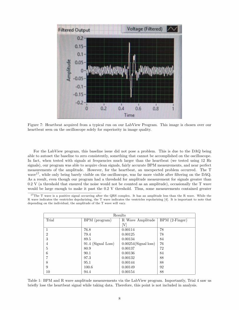
Figure 7: Heartbeat acquired from a typical run on our LabView Program. This image is chosen over ourheartbeat seen on the oscilloscope solely for superiority in image quality.

For the LabView program, this baseline issue did not pose a problem. This is due to the DAQ beingable to autoset the baseline to zero consistently, something that cannot be accomplished on the oscilloscope.In fact, when tested with signals at frequencies much larger than the heartbeat (we tested using 12 Hzsignals), our program was able to acquire clean signals, fairly accurate BPM measurements, and near perfectmeasurements of the amplitude. However, for the heartbeat, an unexpected problem occurred. The Twave17, while only being barely visible on the oscilloscope, was far more visible after filtering on the DAQ.As a result, even though our program had a threshold for amplitude measurement for signals greater than0.2 V (a threshold that ensured the noise would not be counted as an amplitude), occasionally the T wavewould be large enough to make it past the 0.2 V threshold. Thus, some measurements contained greater

17The T wave is a positive signal occurring after the QRS complex. It has an amplitude less than the R wave. While theR wave indicates the ventricles depolarizing, the T wave indicates the ventricles repolarizing [4]. It is important to note thatdepending on the individual, the amplitude of the T wave will vary.

ResultsTrial BPM (program) R Wave Amplitude

[V]BPM (2-Finger)

1 76.8 0.00114 782 79.4 0.00125 783 89.5 0.00134 844 91.4 (Signal Loss) 0.00254(Signal loss) 765 80.9 0.00137 726 90.1 0.00136 847 97.3 0.00132 888 95.1 0.00144 889 100.6 0.00149 9210 94.4 0.00154 88

Table 1: BPM and R wave amplitude measurements via the LabView program. Importantly, Trial 4 saw usbriefly lose the heartbeat signal while taking data. Therefore, this point is not included in analysis.

8

than the anticipated heartbeats per sample18 due to the strength of the T wave, resulting in an inaccurateBPM measurement and R wave amplitude. In addition, another less major issue we encountered was thatif the signal was not getting picked up very well by the electrodes, then some of the R wave peaks wouldnot cross the 0.2 V threshold, thus causing our measurements to contain less than 10 heartbeats per sample.However, this issue was easy to alleviate simply by readjusting the electrodes or changing their placement inorder to get a better signal. Similarly, there was a slight correlation in the quality of the signal and whetheror not the T wave would cross the threshold (better quality signals were more likely to measure the expectednumber of heartbeats per sample at the R wave peak). This observation led us to believe that the T wavewas getting artificially amplified if the signals were of lower quality.

To solve the T wave anomaly, we decided to count heartbeats using the S wave rather than the R wave(the R wave was still used to measure the amplitude of the heartbeat). The reason for this was that since theR and T waves are both positive while the S wave is negative, and since the S wave is the only large negativespike during the heartbeat, there is no conflict in measuring the beats using this wave since no other wavewould pass the S wave’s threshold. Additionally, since the heartbeat is very consistent, the measured periodbetween beats would not change if measured from the S or R wave. In lieu of this, we created a new path tomeasure the heartbeat times by measuring the time at which the S wave forms a valley, once again settinga threshold above the noise (∼ -0.2 V). However, since the S wave was a bit noisy, some double peaks werebeing counted as the peak of the S wave had some noise that caused to to briefly fluctuate at the thresholdsetting. Given that these double peaks were always less than 0.01 s from the true peak, we were able to fixthis issue by including a nested for loop with shift registers and a case structure. The for loop would iterateover each period value between beats and the case structure would append measurements above 0.1 s to theshift register, thus eliminating the double peaks. The result allowed our BPM program to be consistentlyaccurate at measuring.

As an example, Table 1 presents the results of 10 trials measuring my BPM and R wave amplitude(adjusted for the gain of the instrumentation amplifier). Note that Trials 1-5 and 6-10 were at differenttimes, hence the large change in BPM. Before running our program for each trial, I measured my own BPMusing the quick two finger test. It is important to note that at Trial 4, the heartbeat signal was briefly lostfor around 2 seconds while taking the measurement. As seen, if the signal is not present for the full durationof the sample, then the measurement can become fairly inaccurate, as Trial 4 measured 91.4 BPM with aself-measured BPM of 76. Additionally, Trial 4 shows how much the measurement for R wave measurementcan be thrown off due to signal loss, as the measurement was much larger than the rest of the sample. Trial4 is kept to show an example of the importance of acquiring a clean signal when using our BPM program;however, it is not included in subsequent analysis. For the 9 other trials, the average BPM using our programwas found to be 81.65 ± 4.76 for trials 1-5 and 95.50 ± 3.46 for trials 6-10. When compared with the twofinger self-measured BPM, an average of 78 ± 4 and 88 ± 3 is calculated for trials 1-5 and 6-10 respectively.It is important to note that error margins on the two-finger measurements are only lower bounds due tothis method of finding a BPM being understandably inaccurate. In comparing our program’s data with thismethod, we see that the averages are reasonably close. Importantly, if we neglect the inaccuracy of the two-finger test and define it to be my actual BPM, our BPM is accurate to ∼6.6% (found by averaging percenterrors of 4.68% and 8.52% for trials 1-5 and 6-10 respectively), confirming that it is reasonably accurate atmeasuring BPM.

6 Conclusion

Our exploration of the efficiency of our ECG was rather successful. Despite some issues with consistencyand a lack of control of acquisition from the electrodes, we were able to attain a signal capable to poweringa LED and speaker in tune with the heartbeat. Additionally, our DAQ and analysis via LabView was ableto generate an accurate BPM and R wave amplitude measurement as long as the acquired signal was of highenough quality. Our main issues regarded the quality of the acquired signal. Even though our LED andspeaker circuit were able to consistently indicate our heartbeats, it was not very consistent in doing what wedesigned it to do. For both the LED and speaker, we intended the LED to flicker just once for when the Rwave would spike positive and the speaker to function similar to professional ECGs seen in hospitals, with

18A sanity check that we included in our program was indicating the size of the array of R wave peak measurements. Anaccurate measurement should have this size be equal to the number of beats seen on the graph. If the size was greater than thecounted number of heartbeats on the waveform, then it meant that the T wave had crossed the 0.2 V threshold and was beingcounted as a peak.

9

beeps to indicate the heartbeat. Instead, we were able to get an LED that would only sometimes turn allthe way off when not positive and a speaker that mostly outputted a constant audio signal that turned off atthe R wave peak. Similarly, our LabView program and DAQ were heavily dependent on the quality of oursignal, causing us to discard samples that featured low quality signals that gave inaccurate measurements asa result.

Due to the issues described above, there are many possible improvement to our ECG. The first and mostobvious improvement would be to get high quality electrodes. Obviously, pennies and dimes are not the bestelectrodes, and our actual electrodes ended up being difficult to solder, likely leading to some extra error inmeasurement. Using high quality electrodes, perhaps electrodes with wires already properly attached wouldlead to better signal acquisition and less noise. Furthermore, most ECGs in practice use far more electrodes(the standard seems to be 12 lead ECGs with 12 electrodes [1], [4]). Since our ECG only utilized 2 (3 withself-grounding), it is reasonable to hypothesize that the signal we were receiving was likely the best thatcould have been achieved. That being said, using more and better quality electrodes would likely have givenus a better signal.

Another possible improvement would be using a different type of bandpass filter. While a typical RCfilter probably would not be better than the Sallen-Key filters that we used, it is possible that either theChebyshev or Butterworth filters would have been better. The Sallen-Key filters that we used were mostlyincluded out of convenience, and since these filters are reliable as shown in Lab 7 [5], they figured to be theideal choice. The Chebyshev filter was briefly discussed introduction, and concerns exist to how much theripples would effect the measurement. The Butterworth filter was only utilized in the LabView filtering. Inthe future, it would be useful to compare directly how well each of these filters performs. The most idealfilter for our ECG would be one with sharp cutoff frequencies, and more comparisons would have been usefulin determining which filter would be most ideal.

Regardless of approach, I consider our ECG successful in that it was able to generate a signal strongenough to be indicated by an LED and speaker and high enough in quality to perform a fairly accurate BPMand R wave measurement on.

7 Acknowledgments

I would like to thank the UC Berkeley Department of Physics for providing us with the resources necessaryto build this project. In addition, I would like to thank Professor Joel Fajans, Dr. Waqas Khalid, and GSIsAdrianne Zhong, Jose Soria, and Kai Isaak-Ellers for their help and guidance in the design and troubleshootingof this project.

References

[1] Frank G. Yanowitz, MD. Professor of Medicine. University of Utah School of Medicine,https://ecg.utah.edu/lesson/3

[2] National Heart, Lung, and Blood Institute. National Institutes of Health. November 17, 2011.,https://www.nhlbi.nih.gov/health-topics/how-heart-works

[3] Flowers NC, Hand RC, Orander PC, Miller CB, Walden MO, Horan LG (March 1974). ”Surface recordingof electrical activity from the region of the bundle of His”. The American Journal of Cardiology.https://www.sciencedirect.com/science/article/pii/0002914974903208

[4] ACLS Medical Training. The Basics of the ECG.https://www.aclsmedicaltraining.com/basics-of-ecg/

[5] Donald A. Glaser Advanced Lab: Instrumentation Laboratory. Labs: 4,5,6,7,8,9http://instrumentationlab.berkeley.edu/labassignments

10