Embed Size (px)
Citation preview
Physics 151 - Mechanics
Taught by Arthur JaffeNotes by Dongryul Kim
Fall 2016
This course was taught by Arthur Jaffe. We met on Tuesdays and Thursdaysfrom 11:30am to 1:00pm in Jefferson 356. We did not use a particular text-book, and there were 17 students enrolled. Grading was based on two in-classmidterms and six assignments. The teaching follow was David Kolchmeyer.
Contents
1 September 1, 2016 41.1 Three conservation laws . . . . . . . . . . . . . . . . . . . . . . . 4
2 September 6, 2016 62.1 More on elliptical orbits . . . . . . . . . . . . . . . . . . . . . . . 62.2 Kepler’s laws . . . . . . . . . . . . . . . . . . . . . . . . . . . . . 62.3 Hyperbolic orbits . . . . . . . . . . . . . . . . . . . . . . . . . . . 7
3 September 8, 2016 83.1 The Rutherford scattering . . . . . . . . . . . . . . . . . . . . . . 8
4 September 13, 2016 94.1 Newton’s equation in coordinates . . . . . . . . . . . . . . . . . . 94.2 The Lagrangian . . . . . . . . . . . . . . . . . . . . . . . . . . . . 104.3 Tensors . . . . . . . . . . . . . . . . . . . . . . . . . . . . . . . . 10
5 September 15, 2016 125.1 Coordinate independence of the Lagrangian . . . . . . . . . . . . 12
6 September 20, 2016 146.1 The Lagrangian in fields . . . . . . . . . . . . . . . . . . . . . . . 146.2 Lagrange’s equation with constraints . . . . . . . . . . . . . . . . 14
7 September 22, 2016 177.1 Calculus of variations . . . . . . . . . . . . . . . . . . . . . . . . 17
1 Last Update: August 27, 2018
8 September 27, 2016 198.1 Least action principle for the oscillator . . . . . . . . . . . . . . . 19
9 September 29, 2016 219.1 The Hamiltonian . . . . . . . . . . . . . . . . . . . . . . . . . . . 219.2 Symmetry and Noether’s theorem . . . . . . . . . . . . . . . . . . 22
10 October 4, 2016 2410.1 Legendre transformation . . . . . . . . . . . . . . . . . . . . . . . 24
11 October 13, 2016 2611.1 Oscillations . . . . . . . . . . . . . . . . . . . . . . . . . . . . . . 26
12 October 18, 2016 2712.1 Hamilton equations for the oscillator . . . . . . . . . . . . . . . . 27
13 October 20, 2016 2913.1 Poisson brackets . . . . . . . . . . . . . . . . . . . . . . . . . . . 29
14 October 25, 2016 3114.1 Examples of canonical transformations . . . . . . . . . . . . . . . 31
15 October 27, 2016 3315.1 Symmetry in elliptical orbits . . . . . . . . . . . . . . . . . . . . 33
16 November 1, 2016 35
17 November 3, 2016 3717.1 Lagrange equations for fields . . . . . . . . . . . . . . . . . . . . 3717.2 Noether’s theorem again . . . . . . . . . . . . . . . . . . . . . . . 38
18 November 8, 2016 3918.1 The energy-momentum density . . . . . . . . . . . . . . . . . . . 39
19 November 10, 2016 4119.1 Solitons . . . . . . . . . . . . . . . . . . . . . . . . . . . . . . . . 41
20 November 15, 2016 4320.1 Target space symmetry . . . . . . . . . . . . . . . . . . . . . . . 4320.2 Topological conservation law . . . . . . . . . . . . . . . . . . . . 44
21 November 17, 2016 4521.1 Review for the exam—lots of examples . . . . . . . . . . . . . . . 45
22 November 29, 2016 4722.1 The Feynman formula . . . . . . . . . . . . . . . . . . . . . . . . 47
2
23 December 1, 2016 5023.1 The Heisenberg equation . . . . . . . . . . . . . . . . . . . . . . . 50
3
Physics 151 Notes 4
1 September 1, 2016
This class is about classical mechanics, but this is actually going to be an intro-duction to theoretical physics. There is a correspondence between conservationlaws and symmetry, which was discovered by Noether, and this has connectionswith mechanics, quantum mechanics, and pure mathematics.
Let us look at a classical problem. Suppose we have a point particle µ at ~rmoving under a central force ~F = −k/r2. I’m going to write ~r = r~n where r isthe magnitude and ~n is the unit vector. The question is: What is the orbit? Thestandard answer is to use Newton’s Law and solve the corresponding differentialequation. What I am going to do today is to answer the same equation withconservation laws.
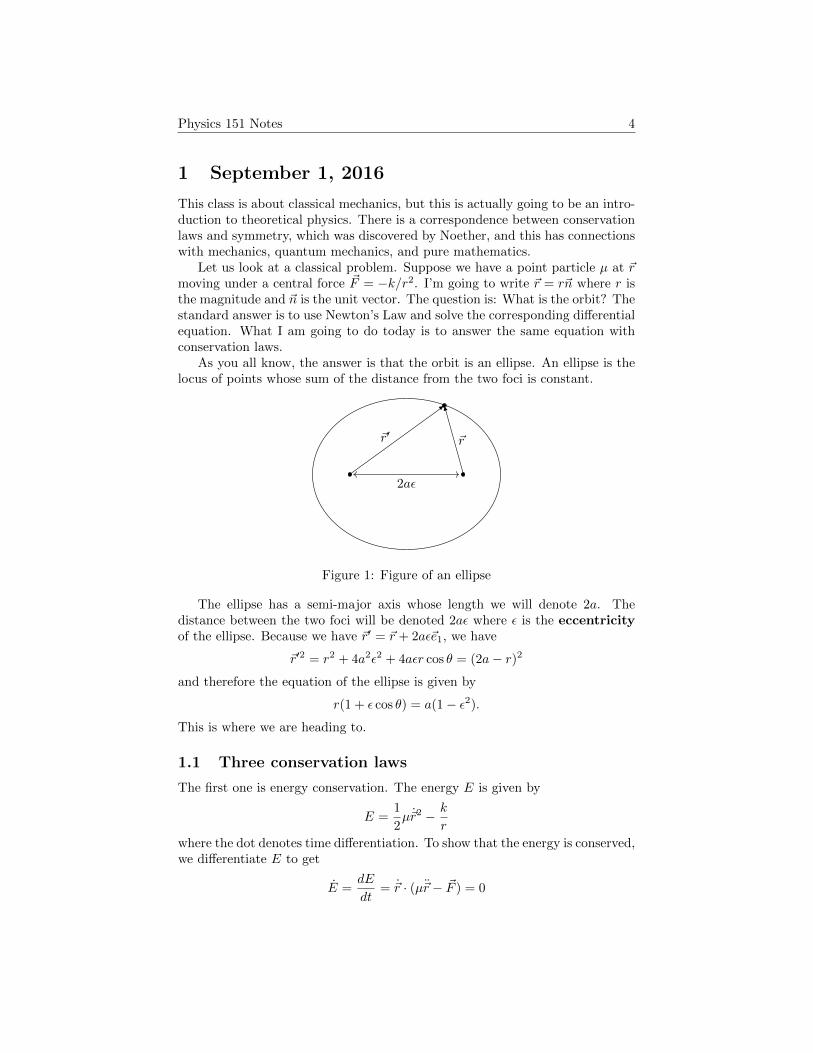
As you all know, the answer is that the orbit is an ellipse. An ellipse is thelocus of points whose sum of the distance from the two foci is constant.
2aε
~r′ ~r
Figure 1: Figure of an ellipse
The ellipse has a semi-major axis whose length we will denote 2a. Thedistance between the two foci will be denoted 2aε where ε is the eccentricityof the ellipse. Because we have ~r′ = ~r + 2aε~e1, we have
~r′2 = r2 + 4a2ε2 + 4aεr cos θ = (2a− r)2
and therefore the equation of the ellipse is given by
r(1 + ε cos θ) = a(1− ε2).
This is where we are heading to.
1.1 Three conservation laws
The first one is energy conservation. The energy E is given by
E =1
2µ~r2 − k
r
where the dot denotes time differentiation. To show that the energy is conserved,we differentiate E to get
E =dE
dt= ~r · (µ~r − ~F ) = 0
Physics 151 Notes 5
by Newton’s law.Item number two is angular momentum around the origin. The angular
momentum ~L is given by ~r × ~p so
d~L
dt= ~r × ~p+ ~r × ~F = 0 + 0 = 0.
From this we can conclude that the motion lies on the plane perpendicular to~L.
The third one is the highlight of this lecture. Energy and angular momentumare general conservation laws that come over everywhere, but this is specific tothe 1/r2 potential. We define the Lenz vector ~ε as
~ε =~p× ~Lµk
− ~n.
This is a dimensionless vector. But why is this conserved? The only things thatchange in this formula are ~p and ~n. We know well what the derivative of ~p is.The derivative of ~n is given as
~n = − 1
r2~n× (~r × ~r).
If this formula is correct, then
~ε =~F × ~Lµk
− ~n = − kµ
r2µk~n× (~r × ~r)− ~n = 0
and hence ~ε is conserved.Now once we have this, we immediately get the orbit. The quantity
~ε · ~r =L2
µk− r = εr cos θ
is conserved. This is precisely the equation of the ellipse. In fact, you even seewhy I named it ε; the magnitude of the Lenz vector is precisely the eccentricityof the orbit.
Physics 151 Notes 6
2 September 6, 2016
There is going to be sections on Mondays at 6:30 at Lyman 330. There is goingto be a dinner tonight in Lowell House Small Dining Room at 5:50.
2.1 More on elliptical orbits
We looked at the orbit of the planet last time. There were three quantities thatare conserved.
(1) Energy - E = 12µ~r
2 − k/r
(2) Angular momentum - ~L = ~r × ~p(3) The Lenz vector - ~ε = ~p× ~L/µk − ~n
Actually I cheated a bit last time. When we derived the formula r(1 +ε cos θ) = L2/µk, I set θ to be the angle between ~r and ~ε. But in the formula,we let θ to be the angle between ~r and ~e1. So we need to check that ~ε and ~e1
have the same direction.1 Because ~ε is constant, we can simply evaluate ε at afew points. On the point on the right, we see that both ~p × ~L and ~n points inthe +e1 direction. On the point on the top, we see that ~p× ~L points in the +e2
direction and ~n points in the slightly −e1 direction. So ~ε will point in the +e1
direction.What about the magnitude of ε? We have
ε2 = ~ε · ~ε = 1 +(~p× ~L
µk
)2
− 2~r · (p× ~L)
µkr= 1 +
p2L2
µ2k2− 2L2
µkr
= 1 +2L2
µk2
( p2
2µ− k
r
)= 1 +
2L2E
µk2.
One remark is that you can get the energy levels of the hydrogen atom from thisformula. Also since ε = 0 for the circle, you can get the energy of the circularorbit.
2.2 Kepler’s laws
What are Kepler’s laws?
1. Elliptical Motion
2. ~r sweeps out equal area in equal time. This comes from the equation
dA
dt=
1
2r2 dθ
dt=
1
2r2θ =
L
2µ.
3. The square of the period τ2 is proportionate to a3. This is actually nottrue, but approximately true if mM .
1I personally don’t understand this. Can’t we set the coordinate system in the first placeso that ~ε aligns with ~e1.
Physics 151 Notes 7
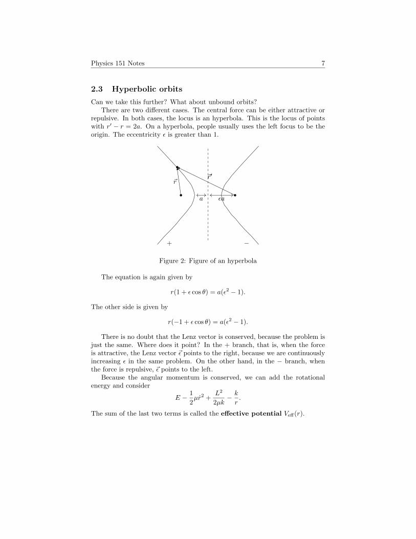
2.3 Hyperbolic orbits
Can we take this further? What about unbound orbits?There are two different cases. The central force can be either attractive or
repulsive. In both cases, the locus is an hyperbola. This is the locus of pointswith r′ − r = 2a. On a hyperbola, people usually uses the left focus to be theorigin. The eccentricity ε is greater than 1.
+ −
a εa
~r~r′
Figure 2: Figure of an hyperbola
The equation is again given by
r(1 + ε cos θ) = a(ε2 − 1).
The other side is given by
r(−1 + ε cos θ) = a(ε2 − 1).
There is no doubt that the Lenz vector is conserved, because the problem isjust the same. Where does it point? In the + branch, that is, when the forceis attractive, the Lenz vector ~ε points to the right, because we are continuouslyincreasing ε in the same problem. On the other hand, in the − branch, whenthe force is repulsive, ~ε points to the left.
Because the angular momentum is conserved, we can add the rotationalenergy and consider
E − 1
2µr2 +
L2
2µk− k
r.
The sum of the last two terms is called the effective potential Veff(r).
Physics 151 Notes 8
3 September 8, 2016
3.1 The Rutherford scattering
Today I want to talk about the Rutherford scattering. This is the case of anunbound, repulsive potential. The formula for the hyperbola is given by
r(−1 + εθ) = −L2
µk.
We see that there is a maximal value of θ, and I am going to write it θmax. Fromthe equation, we see that cos θmax = 1/ε. Then
tan θmax =√ε2 − 1 =
√2EL2
µk2.
In the Rutherford experiment, the scattering angle is given by Θ = π−2θmax.Hence we can say that
cotΘ
2=
√2EL2
µk2.
But we need to parameterize in terms of the impact parameter, which is thedistance between the asymptote and the origin. Because the energy and theangular momentum is conserved, we can compute it at large distance. Then wesee that √
2µE = pin, L = spin = s√
2µE.
Then we can write
cotΘ
2=
√2EL2
µk2=
2sE
|k|, s =
|k|2E
cosΘ
2.
To analyze the situation in 3-dimensions, we use spherical polar coordinates(r,Θ, φ). We write Θ to make it match our scattering angle. Here, Θ is theangle between ~r and the +z-axis. The volume form and the area form on theunit sphere are given by
dV = r2dr sin ΘdΘdφ, dΩ = sin ΘdΘdφ.
To see how much of the incoming beam go to the sphere, we divide sdsdφ bydΩ. Then the differential scattering cross section is given by
dσ
dΩ=∣∣∣ sdsdφ
sin ΘdΘdφ
∣∣∣ =s
sin Θ
∣∣∣ dsdΘ
∣∣∣ =( k
4E
)2 1
sin4(Θ/2)
if you plug it in the formula. This is the Rutherford formula.There is actually a big problem. These are atomic particles and thus they
can’t be really described by classical mechanics. But if you actually compute itfor the quantum mechanical picture, you get the same answer.
Physics 151 Notes 9
4 September 13, 2016
Today we are going back to Newtonian mechanics. I want to start by givingexamples.
4.1 Newton’s equation in coordinates
In Cartesian coordinates, ~r = x~e1 + y~e2 + z~e3. Newton’s equation states that~F = m~a where ~a = ~r and ~F = −∇V . If we write it in coordinates,
mx = Fx = −∂F∂x
.
We might want to label x1, x2, . . . , xN where N is 3 times the number of parti-cles.
If we are working in planar coordinates (r, θ) replacing (x, y), so that ~r = r~n
with ~l ⊥ ~n, then we can go back and forth in coordinates as
r =√x2 + y2 x = r cos θ
tan θ =y
xy = r sin θ.
Because we know how to take the derivative in Cartesian coordinates. We have
~r = r~n+ rθ~l,
~r = r~n+ rθ~l + rθ~l + rθ~l − rθ2~n = (r − rθ2)~n+ (2rθ + rθ)~l.
Each of these components of a name: r is the radial acceleration, −rθ2 is thecentripetal acceleration, 2rθ is the Coriolis acceleration, and rθ is the angularacceleration.
Now that we know the acceleration in the components, let us compute thecomponents of the force. We can write
∇V =∂V
∂x~e1 +
∂V
∂t~e2 = (∇V )r~n+ (∇V )θ~l.
The (∇V )r can be computed as
(∇V )r = (∇V ) · ~n =∂V
∂xcos θ +
∂V
∂ysin θ =
∂V
∂x
∂x
∂r+∂V
∂y
∂y
∂r=∂V
∂r.
You have to be careful because each derivative has one variable that changesand one variable that is fixed. Likewise,
(∇V )θ = (∇V ) ·~l = −∂V∂x
sin θ +∂V
∂ycos θ =
1
r
∂V
∂x
∂x
∂θ+
1
r
∂V
∂y
∂y
∂θ=
1
r
∂V
∂θ.
So the Newton equations can be written as
m(r − rθ2) = −∂V∂r
, m(rθ + 2rθ) = −1
r
∂V
∂θ.
This looks very different from what we had in Cartesian coordinates. In factthey are exactly the same equation when we express in terms of the Lagrangian.This is some kind of covariance, or symmetry.
Physics 151 Notes 10
4.2 The Lagrangian
The kinetic energy is given as
T =1
2mx2 +
1
2my2,
and let V = V (x, y) be an arbitrary potential.Newton’s equation gives
−(∂V∂x
)y,x,y
= mx =d
dt
(∂T∂x
)y,x,y
,
−(∂V∂y
)x,x,y
= my =d
dt
(∂T∂y
)x,x,y
.
To make this is simpler, we define the Lagrangian as L = T −V . Then we canrewrite the equation as
d
dt
∂L∂x
=∂L
∂x,
d
dt
∂L∂y
=∂L∂y
.
This is called the Lagrangian’s equation, and this form is independent of coor-dinate system.
Let us look at L in terms of plane polar coordinates. We have
L = T − V =1
2m(r2 + r2θ2)− V (r, θ).
Then the Lagrangian equations are
d
dt(mr) = mrθ2 − ∂V
∂r,
d
dt(mr2θ) = −∂V
∂θ.
This way we didn’t need to go through all the algebra. This is the philosophyof the Lagrangian equation.
4.3 Tensors
Let V (x) with x = (x1, . . . , xN ). Set up a new coordinate x(q) with q =(q1, . . . , qN ). To translate a vector in x coordinates q, we can apply the chainrule and write
∂
∂qiV (x(q)) =
N∑j=1
∂V
∂xj
∂xj∂qi
.
This transformation looks like ~W = J ~W , and things that satisfy this relationare called covariant vectors. There are vectors that transform in the otherdirection, like
dqi =∑j
∂qi∂xj
dxj .
Physics 151 Notes 11
These are called contravariant vectors.The Jacobian is defined as
Jij =(∂xj∂qi
)q1,...,6qi,...,qN
.
This must be invertible, because the coordinate transform must be invertible inthe first place. The inverse will be given by
Jij =(∂qj∂xi
)x1,...,6xi,...,xN
.
Then JJ = I = JJ .
Physics 151 Notes 12
5 September 15, 2016
Suppose there are functions of coordinates q = (q1, . . . , qN ) and q = q(q′). LetVi be functions of coordinates q, nad V ′i be functions of q′ with V ′i = Vi(q(q
′)).We are going to say that Vi is a covariant vector if these satisfy the relation
V ′i =
N∑j=1
∂q′jqiVj .
5.1 Coordinate independence of the Lagrangian
The Lagrangian is given as L = T − V where T = T (x, x, t) and V = V (x, t).We are assuming that the potential is only dependent on the position, i.e., thisis not like the system of a charged particle in a magnetic field. Let q be anothercoordinates with x = x(q). We are going to derive
d
dt
∂L∂qi− ∂L∂qi
= 0 fromd
dt
∂L∂xi− ∂L∂xi
= 0.
To make simple, let us take out the time-dependence of L. Consider
∂L(x(q), x(q, q))
∂qi=
N∑j=1
∂L∂xj
∂xj∂qi
+
N∑j=1
∂L∂xj
∂xj∂qi
.
This doesn’t work by itself, and so let us compute the other term. Before this,we note that
xi(q, q) =d
dtxi(q) =
N∑j=1
∂xi∂qj
dqjdt
=
N∑j=1
(∂xi∂qj
)qj ,
so it follows that
∂xi∂qj
=∂xi∂qj
.
This is called the cancellation of dots. The other term in Lagrange’s equationis
d
dt
∂L∂qi
=d
dt
N∑j=1
(∂L∂xj
∂xj∂qi
+∂L∂xj
∂xj∂qi
)=
d
dt
N∑j=1
∂L
∂xj
∂xj∂qi
=
N∑j=1
(d
dt
∂L∂xj
)∂xj∂qi
+
N∑j=1
∂L∂xj
(d
dt
∂xj∂qi
).
Then the difference is
d
dt
∂L∂qi− ∂L∂qi
=
N∑j=1
(d
dt
∂L∂xj− ∂L∂xj
)∂xj∂qi
+
N∑j=1
∂L∂xj
(d
dt
∂xj∂qi− ∂xj∂qi
).
Physics 151 Notes 13
The second term is zero because
∂xj∂qi
=
N∑l=1
∂2xj∂ql∂qi
ql,d
dt
∂xj∂qi
=
N∑l=1
∂2xj∂ql∂qi
ql.
So what we are left with is(d
dt
∂L∂qi− ∂L∂qi
)=
N∑j=1
(d
dt
∂L∂xj− ∂L∂xj
)(∂xj∂qi
).
If we write the Lagrange vector V Lag and Newton vector V New as
V Lagi =
d
dt
∂L∂qi− ∂L∂qi
, V Newi =
d
dt
∂L∂xi− ∂L∂xi
,
then what we have just proved can be written as
V Lag = JV New.
Now if Newton’s Equations are correct, then V New = 0. It follows from theformula that V Lag = 0.
Physics 151 Notes 14
6 September 20, 2016
Let me start with a bit of review. For the Lagrangian L(q, q, t), we have
d
dt
∂L∂qi− ∂L∂qi
= 0.
In this equation, pi = ∂L/∂qi is called the generalized momentum andFi = ∂L/∂qi is called the generalized force. For instance, if
T =1
2
∑miq
2i , V = V (q)
then pi = miqi and if
T =1
2mr2 +
1
2mr2θ2, V = V (r, θ)
then pr = mr and pθ = mr2θ. This pθ is the angular momentum L. If we lookonly at the dimension, then
[pi][qi] = [pi][qi]T = [L]T = [Action].
6.1 The Lagrangian in fields
Take a charged particle in coordinate ~x(t) with charge e. The electric andmagnetic field can be written as
~B(~x, t) = ∇× ~A(~x, t), ~E = −∇Φ(~x, t)− ∂ ~A
∂t
where Φ and ~A are scalar and vector potentials. We can write down the La-grangian of this charge as
L =1
2m~x2 − eΦ(~x, t) + e
3∑j=1
Aj(~x, t)xj(t).
What are the Lagrange equations for this? After a bit of algebra, you will get
m~x = e( ~E + ~x× ~B).
This is the Lorentz force. That Lagrangian is the minimal coupling.
6.2 Lagrange’s equation with constraints
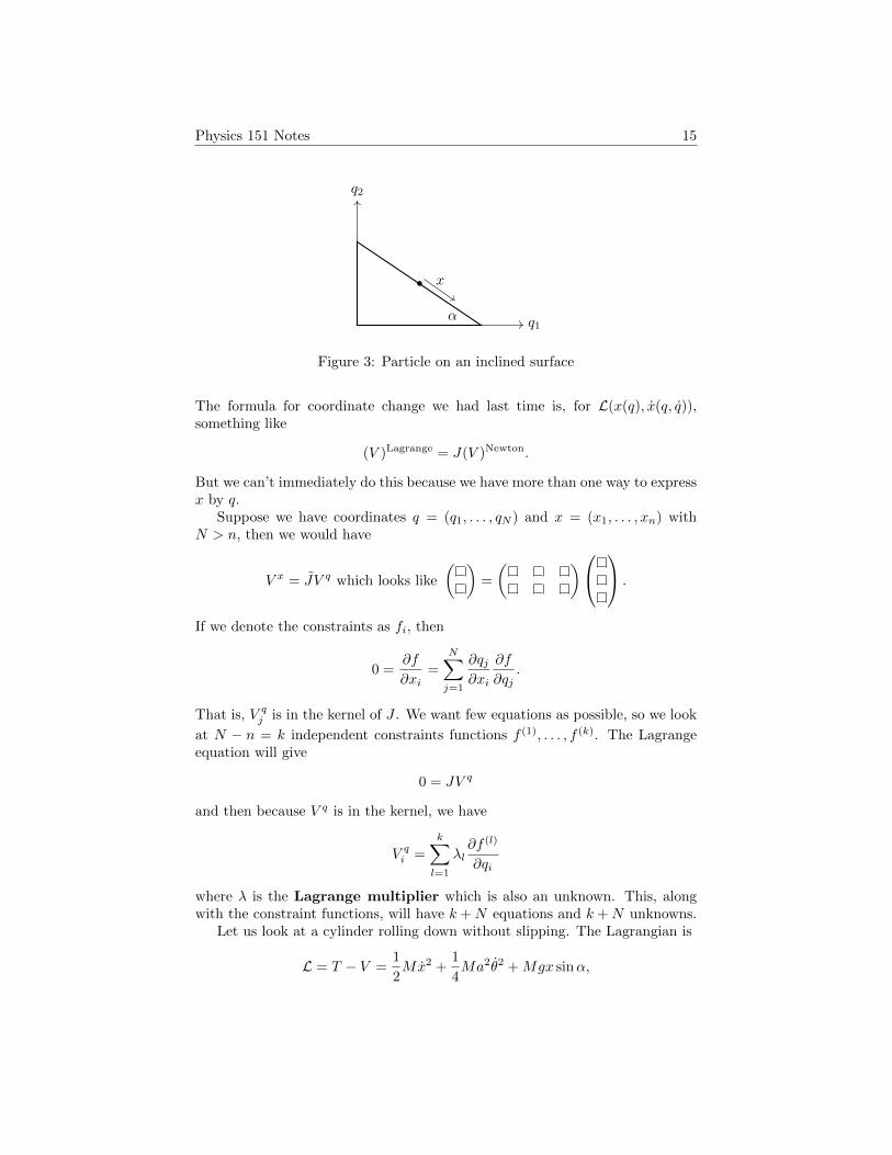
Sometimes it is useful to introduce redundant coordinates. For instance, con-sider a particle on a inclined surface. In this case, we have q1 = x cosα andq2 = −x sinα. So to be on the plane, we need a constraint
f(q1, q2) = q1 tanα+ q2 = 0.
Physics 151 Notes 15
q1
q2
α
x
Figure 3: Particle on an inclined surface
The formula for coordinate change we had last time is, for L(x(q), x(q, q)),something like
(V )Lagrange = J(V )Newton.
But we can’t immediately do this because we have more than one way to expressx by q.
Suppose we have coordinates q = (q1, . . . , qN ) and x = (x1, . . . , xn) withN > n, then we would have
V x = JV q which looks like
( )=
( ) .
If we denote the constraints as fi, then
0 =∂f
∂xi=
N∑j=1
∂qj∂xi
∂f
∂qj.
That is, V qj is in the kernel of J . We want few equations as possible, so we look
at N − n = k independent constraints functions f (1), . . . , f (k). The Lagrangeequation will give
0 = JV q
and then because V q is in the kernel, we have
V qi =
k∑l=1
λl∂f (l)
∂qi
where λ is the Lagrange multiplier which is also an unknown. This, alongwith the constraint functions, will have k +N equations and k +N unknowns.
Let us look at a cylinder rolling down without slipping. The Lagrangian is
L = T − V =1
2Mx2 +
1
4Ma2θ2 +Mgx sinα,
Physics 151 Notes 16
and the constraint is f = x− aθ. Then the equations are
d
dt
∂L∂x− ∂L∂x
= λ∂f
∂x,
d
dt
∂L∂θ− ∂L
∂θ= λ
∂f
∂θ, f = 0.
These are three equations in three unknowns x, θ, λ. Explicitly,
Mx−Mg sinα = λ,1
2Ma2θ = −λa, x = aθ.
Then you can get (3/2). . . x = g sinα. In this case, λ = −(1/3)Mg sinα, and
this you can interpret as the force of the constraint.To sum up, the Lagrange’s equations are
d
dt
∂L∂qi
=∂L∂qi
+
k∑j=1
λj∂f (j)
∂qi.
These type of constraints are called holonomic constraints.
Physics 151 Notes 17
7 September 22, 2016
7.1 Calculus of variations
If we have a function f , then the maxima and minima are attained at the pointswhere f ′ is zero. If f has more that one component, i.e., take a vector, there aremany choices of directions in which we can take the derivative. For a directionη, the directional derivative is
(D~ηf)(~x) = limε→0
f(~x+ ε~η)− f(~x)
ε= (∇f) · ~η.
A more complicated situation is where ~x is not a point in Euclidean space buta function. In mechanics, this comes in as f being the Lagrangian. Let x beq(t) = (q1(t), . . . , qN (t)) for tA ≤ t ≤ tB . We define the action as
Saction =
∫ tB
tA
L(q(t), q(t), t)dt = S(q).
This S now plays the role of f with q playing the role of x. To analyze thissituation, we must ask what it means to differentiate a function over a function.
Let us define the derivative of S(q). As in the case of a function over vectors,the most natural thing is to look at the directional derivatives. For anotherfunction η = (η1(t), . . . , ηN (t)), the directional derivative of S(q) will be
(DηS)(q) = limε→0
S(q + εη)− S(q)
ε.
Because we have a definition of S, we can straightforwardly compute it as
(DηS)(q) = limε→0
∫ tB
tA
L(q(t) + εη(t), q(t) + εη(t), t)− L(q(t), q(t), t)
εdt
=
∫ tB
tA
N∑j=1
(∂L∂qj
ηj(t) +∂L∂qj
ηj(t)
)dt.
Let us additionally require the endpoints are fixed, i.e., η(tA) = η(tB) = 0. Ifthis is true, then
∂L∂qj
=d
dt
( ∂L∂qj
ηj(t))− d
dt
∂L∂qj
ηj(t).
So we can continue the expression using this identity as
(Dη)(q) =
∫ tB
tA
N∑j=1
(∂L∂qj
ηj(t) +∂L∂qj
ηj(t)
)dt
=
∫ tB
tA
N∑j=1
(∂L∂qj− d
dt
∂L∂qj
)ηj(t)dt+
∫ tB
tA
N∑j=1
d
dt
(∂L∂qj
ηj(t)
)dt
=
∫ tB
tA
N∑j=1
(∂L∂qj− d
dt
∂L∂qj
)ηj(t)dt = 〈V Lag, η〉.
Physics 151 Notes 18
Now Hamilton’s principle says that (DηS)(Q) for all η if and only if V Lag(Q) =0. The backward direction is trivial. For the forward direction, let ηj(t) to bethe same as ∂L/∂qj − (d/dt)(∂L/∂qj). Then the integral becomes the integralof some nonnegative functions, and so it must be zero.
Physics 151 Notes 19
8 September 27, 2016
The principle of least action says that the Lagrangian equations come fromminimizing action S(q) with fixed endpoints for q.
8.1 Least action principle for the oscillator
For example, consider the harmonic oscillator in one dimensions, whose equationis given by q(t) = −ω2q(t) for t1 ≤ t ≤ t2. The solution to this equation is
Q(t) = Q(t1) cos(ω(t− t1)) +Q(t1)
ωsin(ω(t− t1)).
The action of q is
S(q) =1
2
∫ t2
t1
(q(t)2 − ω2q(t)2)dt.
In terms of the position at the two endpoints, the solution can be written as
Q(t) = Q(t1)(
cos(ω(t− t1))− cos(ω(t2 − t1))
sin(ω(t2 − t1))sin(ω(t− t1))
)+Q(t2)
sin(ω(t− t1))
sin(ω(t2 − t1)).
If sin(ω(t2 − t1)) = 0, then some problem occurs, and you can even see thisphysically; the two endpoints does not determine the solution.
Now let Q(t) be the solution to the Euler-Lagrange equations and η(t) be avariation with vanishing endpoints at t1 and t2. Let q = Q+ η. Then
S(q) = S(Q) + S(η) +
∫ t2
t1
(Qη − ω2Qη)dt
= S(Q) + S(η) +
∫ t2
t1
(−Qη − ω2Qη)dt = S(Q) + S(η).
This means that the principle of least action for the harmonic oscillator is aquestion whether S(η) ≥ 0. We have
S(η) =1
2
∫ t2
t1
(η(t)2 − ω2η(t)2)dt
If we find any η that makes S(η) < 0, then the principle of least action is false.To make η small and η big, we consider the function η(t) = sin(π(t−t1)/(t2−t1)).Then
S(t) =1
2
∫ t2
t1
(η(t)2 − ω2η(t)2)dt =1
2
(( π
t2 − t1
)2
− ω2) t2 − t1
2.
Physics 151 Notes 20
So S(η) > 0 if t2 − t1 < π/ω, for my specific choice of η. On the other hand ift2− t1 > π/ω then the action is not minimized. This shows that if t2− t1 > π/ωthe principle of least action is false.
What if we integrate S(η) by parts? Then
S(η) =1
2
∫ t2
t1
η(t)(− d2
dt2− ω2
)η(t)dt =
1
2
⟨η,( d2
dt2− ω2
)η⟩.
So this is in fact an eigenvalue problem.Let us write down the normalized eigenvectors. These will be
f (n)(t) =
√2
t2 − t1sin(π(t− t1)n
t2 − t1
)with λn =
( π
t2 − t− 1
)2
n2 − ω2.
Moreover, if n1 6= n2 then 〈f (n1), f (n2)〉 = δn1n2.
In fact f (n)(t) are a basis and everything can be expanded in terms of thesef (n). If
η(t) =
∞∑j=1
cjf(j)(t)
then
S(η) =
∞∑j=1
c2j
( π2
(t2 − t1)2j2 − ω2
).
Then whether S(η) ≥ 0 for all η reduces to the question of whether π2/(t2 −t1)2j2 > ω2 for all j. That is, it is related to the smallest eigenvalue of thetransformation.
Physics 151 Notes 21
9 September 29, 2016
9.1 The Hamiltonian
The quantity
H =
N∑j=1
piqi − L(q, q, t)
is called the Hamiltonian and plays an important role.So far, we have look at the case when the Lagrangian takes the form of
L = T − V, T =1
2
N∑i,j=1
tij(q)qiqj , V = V (q),
where tij = tji are the coefficients. The pis are defined as
pi =∂L∂qi
=
N∑j=1
tij(q)qj .
In this case,
N∑i=1
qipi =
N∑i,j=1
qitij(q)qj = 2T.
So H = T +V . This is why the Hamiltonian is generally identified with energy.Let us calculate the time derivative of H along a trajectory satisfying La-
grange’s equation. First
dLdt
=
N∑i=1
(∂L∂qi
qi +∂L∂qi
qi
)+∂L∂t
=
N∑i=1
(piqi + piqi) +∂L∂t
=d
dt
N∑i=1
piqi +∂L∂t.
So
dH
dt= −∂L
∂t
if we go along the trajectory that satisfies the Lagrangian equation. So H isconstant if L is time-independent.
The Lagrangian for the relativistic particle is given by
L = −mc2√
1−(vc
).
Physics 151 Notes 22
Note that for small v, this is −mc2 + 1/2mv2 +O(v4). The momentum can becomputed as
pi =∂L∂vi
=mvi√1− β2
where β =v
c.
The Hamiltonian is then
H = ~p · ~v − L =√p2c2 +m2c4
after some algebra.
9.2 Symmetry and Noether’s theorem
What is a symmetry? We are going to consider a family of transformations qε,and consider the Lagrangian L(qε, qε, t). For instance, Let xε be the rotation byε about axis ~n of x. We are then going to ask whether L stays the same underthe rotation.
For example, take
L(x, x, t) =1
2m(x2
1 + x22 + x2
3)− 1
2(k1x
21 + k2x
22 + k3x
23).
The rotation is a symmetry for the kinetic energy, and if the potential energyis also conserved under coordinate change, then this rotation is a symmetry ofL. Noether’s theorem says that every symmetry is associated to a conservationof a quantity.
Theorem 9.1 (Noether’s theorem 1). If L(q, q, t) = L(qε, qε, t) for a family qεdifferentiable in ε near ε = 0, and identity ε = 0, then the quantity
Q =
N∑i=1
pidqε,idε
∣∣∣ε=0
is conserved.
Proof. We have
0 =d
dεL(qε, qε, t) =
N∑i=1
(∂L∂qε,i
dqε,idε
+∂L∂qε,i
dqε,idε
)=
N∑i=1
(pε,i
dqε,idε
+ pε,idqε,idε
).
This is just dQ/dt = 0.
Consider the system with two particles ~x(1) and ~x(2). The kinetic energy isgiven by
T =1
2M ~R2 +
1
2µ~r2.
Physics 151 Notes 23
Consider new coordinates ~x(1)ε = ~x(1)+ε~a and ~x
(2)ε = ~x(2)+ε~a. Then ~Rε = ~R+ε~a
and ~rε = ~r. So the kinetic energy
T (~Rε, ~Rε, ~rε, ~rε) =1
2M ~R2
ε +1
2µ~r2ε
is the same. So this is a symmetry. In this case,
Q = ~P · ~a = (~p(1) + ~p(2)) · ~a
is conserved.
Physics 151 Notes 24
10 October 4, 2016
Recall that Noether’s theorem 1 states that if q → qε is a family of translationssuch that Lε(q, q, t) = L(qε, qε, t) is equal to L, then the charge
Q =
N∑i=1
pidqεidε
∣∣∣ε=0
is conserved on a trajectory satisfying Lagrange’s equations.There is a generalized version of this theorem.
Theorem 10.1 (Noether’s theorem 2). Suppose there is a function G(q, q, t)such that (d/dε)Lε|ε=0 = dG/dt. Then the charge
Q =
N∑i=1
pidqεidε
∣∣∣ε=0−G
is conserved along a trajectory satisfying Lagrange’s equations.
Proof. To see this, look at
d
dεLε =
N∑i=1
( ∂L∂qεi
dqεidε
+∂L∂qεi
dqεidε
)=
d
dt
( N∑i=1
pεidqεidε
).
Then we immediately get the theorem.
For example, take qεi(t) = qi(t+ ε). Then
d
dεLε(q(t), q(t), t)
∣∣∣ε=0
=d
dεL(q(t+ ε), q(t+ ε), t)
∣∣∣ε=0
=d
dtL(q, q, t)− ∂L
∂t.
In the case of ∂L/∂t = 0, we can choose G = L. In that case,
Q =
N∑i=1
piqi − L = H.
is conserved.
10.1 Legendre transformation
We know how to get H to L. It turns out that it is also possible to obtain Lfrom H, and these transformations are in fact the same transformation. TheLagrangian L is expressed in terms of the varibles q and q, and the Hamiltonianis expressed in terms of q and p.
Example 10.2. Consider the example
L =1
2〈q,Mq〉 − V (q)
for some symmetric matrix M . Then p = Mq and
H(q, p) =1
2〈q,Mq〉+ V (q) =
1
2〈p,M−1p〉+ V (q).
Physics 151 Notes 25
Example 10.3. Consider a particle in a magnetic field. The Lagrangian andmomentum is given by
L =1
2mv2 + e ~A · ~v − V (x), ~p = m~v + e ~A.
So
H = ~p · ~v − L =1
2m|~p− e ~A|2 + V (x)
Because there is a way of writing pi in terms of L and qi, there also has tobe a way of writing qi in terms of H and pi. We have
∂H
∂pi=
∂
∂pi
( N∑j=1
pj qj − L)
= qi +
N∑j=1
(pj∂qj∂pi− ∂L∂qj
∂qj∂pi
)= qi.
This is half of Hamilton’s equations. We also have
∂H
∂qi=
N∑j=1
(pi∂qj∂qi− ∂L∂qj
∂qj∂qi
)− ∂L∂qi
= −pi.
The Hamilton’s equations are
∂H
∂pi= qi,
∂H
∂qi= −pi.
We got off a bit to the side track, but let us get back to the Legendretransform.
Example 10.4. Take a 1-dimensional system with L = (1/2)mv2−V (x). ThenH = pv − L where p = ∂L/∂v = mv. The fact that p = ∂L/∂v implies that vis the maximal point of the function pv − L(x, v) as a function over v. Thus
H(x, p) = pv − L = maxv
(pv − L).
Likewise, because L = pv − H, we have an analogous equation for L in termsof H.
Consider L(v) = vα/α for v > 0 and α > 1. Then
H(p) = maxv
(pv − 1
βpβ for
1
α+
1
β= 1.
As a consequence,
pv ≤ 1
αvα +
1
βpβ
for any p and v. The equality holds when the maximum is attained. This isYoung’s inequality.
Physics 151 Notes 26
11 October 13, 2016
What I want to start on today is Hamilton’s equations.
qi =∂H
∂pi, pi =
∂H
∂qi.
Now we can think the whole thing as a 2N vector
ξ =
q1
...qNp1
...pN
that is in the phase space. Then Hamilton’s equations can be written as
ξ(t) = Γ∇ξH(ξ), Γ =
(0 I−I 0
).
This is just a short-hand notation for Hamilton’s equations.
11.1 Oscillations
Consider a general quadratic Lagrangian
L =1
2〈q,Mq〉 − 1
2〈q,Mq〉,
where are M and K are positive definite symmetric real matrices. These canbe diagonalized with positive eigenvalues, because they are hermitian and thusnormal.2
The Lagrange equations say that
Mq +Kq = 0.
To solve this equation, we let Q = M1/2q and we get M1/2Q = −KM−1/2Q.Then
Q = −M−1/2KM−1/2Q.
Then M−1/2KM−1/2 turns out to be a real symmetric matrix with positiveeigenvalues, and so we can write M−1/2KM−1/2 = Ω2. Then our equation isQ = −Ω2Q. Then we can solve it as
Q(t) = cos(Ωt)Q(0) + Ω−1 sin(Ωt)Q(0).
So the final solution is
q(t) = M−1/2 cos(Ωt)M1/2q(0) +M−1/2Ω−1 sin(Ωt)M1/2q(0).
2These are the matrices that satisfy MM† = M†M .
Physics 151 Notes 27
12 October 18, 2016
Last time we look at the oscillator whose Lagrangian is given by
L =1
2〈Q, Q〉 − 1
2〈Q,Ω2Q〉
where Q = M1/2q and Ω2 = M−1/2KM−1/2. Then the solution is given by
Q(t) = cos(Ωt)Q(0)− Ω−1 sin(Ωt)Q(0).
Suppose f (j) is a normalized eigenvectors of Ω, and let ωj be the frequencies.Write
Q(0) =
N∑j=1
αjf(j), Q(0) =
N∑j=1
βjωjf(j).
Let us compute the Hamiltonian H = 12 〈Q, Q〉+ 1
2 〈Q,Ω2Q〉. We have
1
2〈Q,Ω2Q〉 =
1
2
⟨ N∑j=1
αjf(j),Ω2
N∑k=1
αkf(k)
⟩=
1
2
N∑j=1
α2jω
2j ,
1
2〈Q, Q〉 =
1
2
N∑j,k=1
〈βjωjf (j), βkωkf(k)〉 =
1
2
N∑j=1
β2jω
2j .
This shows that
H =1
2
N∑j=1
(α2j + β2
j )ω2j .
That is, energy is additive over normal modes!
12.1 Hamilton equations for the oscillator
Recall that Hamilton’s equations are
∂H
∂p= q,
∂H
∂q= −p.
The Hamiltonian is given by
H =1
2〈p,M−1p〉+
1
2〈q,Kq〉 =
1
2
⟨ξ,
(K 00 M−1
)ξ
⟩, where ξ =
(qp
).
The Hamilton equations are given by
ξ =
(0 M−1
−K 0
)ξ(t) = Tξ(t).
Physics 151 Notes 28
So the solution is given by
ξ(t) = etT ξ(0).
This solution must agree with the solution we have obtained before. Let uscheck this. It’s easier if we also do the same scale transformation. If we haveQ = M1/2q, then
P =∂L∂Q
= Q = M1/2q = M−1/2p.
So
Ξ =
(QP
)=
(M1/2 0
0 M−1/2
)ξ.
In this new coordinates, the Hamilton equations become
dΞ
dt=
(0 I−Ω2 0
)Ξ = XΞ.
Then
Ξ(t) = etXΞ(0) =
(cos(Ωt) Ω−1 sin(Ωt)−Ω sin(Ωt) cos(Ωt)
)Ξ(0),
and thus
ξ(t) =
(M−1/2 0
0 M1/2
)(cos Ωt Ω−1 sin Ωt−Ω sin Ωt cos Ωt
)(M1/2 0
0 M−1/2
)ξ(0).
Physics 151 Notes 29
13 October 20, 2016
Today we are going to talk about Hamilton’s equation. It is given by
dξ
dt=
(0 I−I 0
)∇ξH.
13.1 Poisson brackets
We can write this as
dξidt
=
( 2N∑j,k=1
Γlj∂H
∂ξj
∂
∂ξl
)ξi.
This is a first order differential equation and in mathematics is called a vectorfield.
The coefficients appear a lot in physics that is given a special name, thePoisson bracket. It is defined as
[A(ξ), B(ξ)]ξ =
2N∑i,j=1
∂A
∂ξiΓij
∂B
∂ξj=
N∑i=1
(∂A
∂qi
∂B
∂pi− ∂A
∂pi
∂B
∂qi
).
So [A,B]ξ = −[B,A]ξ, i.e., the Poisson bracket is skew-symmetric. Using thisnotation, this can be written as
dξidt
= −[H, ξi]ξ.
We also write [A,B]ξ = DAB, and this DA is called the Lie derivative. Thenwe can write dξ(t)/dt = −DHξ(t). Let us look at some examples. Clearly
[qi, qj ]ξ = 0, [pi, pj ]ξ = 0, [qi, qj ] = δij .
These are called the fundamental Poisson brackets. This can be also writtenas [ξi, ξj ]ξ = Γij .
Let us do a change of coordinates and write(qp
)= ξ →
(QP
)= Ξ.
This change of coordinates is said to be canonical if
[Ξi,Ξj ] = Γij .
For example, the scaling transformation Qi = (M1/2q)i and Pj = (M−1/2p)j iscanonical.
The solutions to Hamilton’s equation are actually canonical transformations.We have
ξ(t) = ξ(0)−∫ t
0
dt1DHξ(t1).
Physics 151 Notes 30
Using perturbation theory, we can write this as
ξ(t) = ξ(0)−∫ t
0
dt1DH
(ξ(0)−
∫ t
0
dt2DHξ(t2)
)= · · ·
=
n∑j=0
(−1)j∫ t
0
dt1
∫ t1
0
dt2 · · ·∫ tj−1
0
dtjDH · · ·DHξ(0) +Rn+1.
This is called Dyson’s formula.
Physics 151 Notes 31
14 October 25, 2016
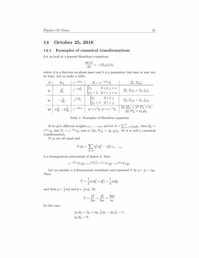
14.1 Examples of canonical transformations
Let us look at a general Hamilton’s equations
dξ(λ)
dλ= −(DAξ)(λ),
where A is a function on phase space and λ is a parameter that may or may notbe time. Let us make a table.
A DA e−λDA Ξi = e−λDAξi [Ξi,Ξk]ξ
qj∂∂pj
e−λ ∂
∂pj
ξi if i 6= j + n
ξi − λ if i = j + n[Ξi,Ξj ]ξ = [ξi, ξj ]ξ
pj − ∂∂qj
eλ ∂
∂qj
ξi if i 6= j
ξi + λ if i = j[Ξi,Ξj ]ξ = [ξi, ξj ]ξ
qp p ∂∂p − q
∂∂q e−λDA q 7→ eλq, p 7→ e−λp
[Q,Q]ξ = [P, P ]ξ = 0,[Q,P ]ξ = [q, p]ξ
Table 1: Examples of Hamilton equations
If we give different weights ω1, . . . , ωN and let A =∑Nj=1 ωjqjpj , then Qj =
eλωjqj and Pj = e−λωjpj and so [Qi, Pj ]ξ = [qi, pj ]ξ. So it is still a canonicaltransformation.
If ωs are all equal and
V (q) =∑|i|=k
qi11 qi22 · · · q
iNN ci1,...,iN
is a homogeneous polynomial of degree k, then
e−λDAV (q) = eλ(∑N
j=1 ij)ωV (q) = eλkωV (q).
Let us consider a 2-dimensional coordinate and represent it by q = q1 + iq2.Then
T =1
2m(q2
1 + q22) =
1
2m ˙qq,
and then p = 12m ˙q and p = 1
2mq. So
T =p2
1
2m+
p22
2m=
2pp
m.
In this case,
[q, p]ξ = [q1 + iq2,12 (p1 − ip2)]ξ = 1,
[q, p]ξ = 0.
Physics 151 Notes 32
So q, q, p, p is also a canonical transformation.We will see later that all solutions to Hamilton’s equations are canonical
transformations. For now, consider the case
H =1
2〈P, P 〉+
1
2〈Q,Ω2Q〉
so that
DH =
N∑i=N
((Ω2Q)i
∂
∂Pi− Pi
∂
∂Qi
)= 〈Q,Ω2 ∂
∂P 〉 − 〈P,∂∂Q 〉.
Physics 151 Notes 33
15 October 27, 2016
In the homework assignment, you have shown that
[Li, Lj ] =∑k
εijkLk
for the angular momentum L of a single particle. The third component isL3 = q1p2 − q2p1 and the Lie derivative is given by
DL3 = −(q1
∂
∂q2− q2
∂
∂q1
)−(p1
∂
∂p2− p2
∂
∂p1
).
Thus
e−θDL3 = eθ(q1∂
∂q2−q2 ∂
∂q1)+θ(p1
∂∂p2−p2 ∂
∂p1).
Note that q1(∂/∂q2) − q2(∂/∂q1) = ∂/∂θ. So DL3is generating a rotation by
the third axis. Likewise, if ~n is a fixed unit vector, then eθD~L·~n is a canonicaltransformation that is the rotation in phase space by θ about ~n.
15.1 Symmetry in elliptical orbits
Suppose we have three functions V1, V2, V3 on phase space that satisfies
[Li, Vj ]ξ =
3∑k=1
εijkVk.
Vj = Lj will be one example, and Vj = qj will also be an example. This isanother way to define a vector in phase space.
In the potential V = −k/r, the vector
~ε =~p× ~Lmk
− ~n
played a special role. This also satisfies [Li, εj ] =∑3k=1 εijkεk. If E < 0 (in the
case of elliptical orbits) define
~K =(−mk
2
2H
)1/2
~ε.
Then K has the same dimension as ~L and
H = − mk2
2(L2 +K2)
by the formula ε2 = 1 + 2EL2/mk2. Then it turns out that
[Li, Lj ]ξ = [Ki,Kj ]ξ =∑k
εijkLk, [Li,Kj ]ξ =∑k
εijkKk.
Physics 151 Notes 34
If we let ~M = (~L+ ~K)/2 and ~N = (~L− ~K)/2, then the above relations can bewritten as
[Mi,Mj ]ξ =∑k
εijkMk, [Ni, Nj ]ξ =∑k
εijkNk, [Mi, Nj ]ξ = 0.
These relations come from the rotational symmetry of the 4-space. In 3-space, there are three rotations coming from,
DL1= q2
∂
∂q3− q3
∂
∂q2, . . .
but in 4-space, there are three more infinitesimal rotations, that can be writtenas
DK1= q4
∂
∂q1− q1
∂
∂q4, DK2
= q4∂
∂q2− q2
∂
∂q4, . . . .
What about unbound orbits? In this case, there is a hyperbolic symmetry.
Physics 151 Notes 35
16 November 1, 2016
Let H = H(ξ) be the Hamiltonian and A(ξ) be a function on phase space. ThenHamilton’s equations tells us that
dA
dt= −DHA = −[H,A]ξ = −
2N∑i,j=1
∂H
∂ξiΓij
∂A
∂ξj.
Then
A(ξ(t)) = e−tDHA(ξ(0))
is the flow on phase space. If [A,H]ξ = 0 then A is conserved by H. If wehave a conserved quantity A, then e−λDAH = H, i.e., the flow generated by aconserved quantity does not change H. Then e−λDA is a symmetry of H.
Example 16.1. Consider the case of Kepler:
H =p2
2µ− k
r.
Because [H,L1]ξ = 0, [H,L2]ξ = 0, it follows from [L1, L2]ξ = L3 that [H,L3]ξ =0. So all angular momentum components are conserved. In this case, we furtherhave symmetries Ki from the rotation of 4-space, SO(4).
Example 16.2. Consider the harmonic oscillator H = p2/2µ+ kr2. The rota-tions does not change the solution, and this can be written as
eθD~L·~ne−tDH ξ = e−tDHe−θD~L·~nξ.
Then DHD~L·~n − D~L·~nDH = D[H,~L·~n] = 0 if ~L is conserved. This means that
[H, ~L · ~n] = 0.
Example 16.3. In the positive energy case of the Kepler problem, we have~K = (mk2/2H)1/2~ε and
[Li, Lj ] =∑
εijkLk, [Ki,Kj ] = −∑
εijkLk, [Li,Kj ] =∑
εijkKk
generates the Lorentz group SO(3, 1).There is a very nice representation of SO(3, 1) by 2× 2 matrices of determi-
nant 1. Note that for any complex matrix A with detA = 1, we can decomposeA = HU for a hermitian matrix H and a unitary matrix U . To see this, justset H = (AA†)1/2 and U = H−1A.
Also there is a correspondence between hermitian matrices and points in4-space as
x = (t, ~x) ↔ tI + x1σ1 + x2σ2 + x3σ3 = x,
Physics 151 Notes 36
where
I =
(1 00 1
), σ1 =
(0 11 0
), σ2 =
(0 −ii 0
), σ3 =
(1 00 −1
).
Then the map x 7→ AxA† gives an action 2 × 2 matrices on 4-space. We canrecover each component by taking xµ = Tr(xσµ)/2. If A is a unitary matrix,then this rotates x1, x2, x3 and leave x0 unchanged. If A is a hermitian matrix,then this gives a boost.
Physics 151 Notes 37
17 November 3, 2016
Consider the classical oscillator given by L = 12 q
2 − 12ω
2q2. There is a fieldanalogue of this. The Klein-Gordon wave equation is given by (+m2)q(t, ~x) =0, where
=∂2
∂t2−∇2 =
∂2
∂t2−
3∑j=1
∂2
∂x2j
.
17.1 Lagrange equations for fields
What does the Lagrangian L look like? Denote x = (t, ~x) and assume
L =
∫Ld~x, S =
∫Ldt =
∫Ldx
where dx = dtd~x. To avoid confusion, let us write ϕ = q and
(∂ϕ)µ =∂ϕ
∂xµfor µ = 1, 2, 3, and (∂ϕ)0 =
∂ϕ
∂t.
Then the Lagrangian density function is given in the form L = L(ϕ, ∂ϕ).Let us use Hamilton’s principle. This means that for any directional deriva-
tive of the action S is 0. Consider a variation ϕ 7→ ϕ(x) + εη(x), such that ηis supported in some set B in space-time. If you compute, it turns out that(DηS)(ϕ) = 0 for all ϕ with fixed boundary conditions at a fixed ϕ, then ϕsatisfies Lagrange’s equations
3∑j=1
( ∂
∂xµ
∂L
∂(∂ϕ)µ
)=∂L
∂ϕ.
Let us show this. We have
Dη = SB(ϕ) = Dη
∫B
Ldx =d
dε
∫L(ϕ+ εη, ∂ϕ+ εdη)dx
∣∣∣∣ε=0
=
∫ (∂L
∂ϕη +
∑µ
∂L
∂(∂ϕ)µ(∂η)µ
)dx
∣∣∣∣ε=0
=
∫B
(∂L
∂ϕ−
3∑µ=0
∂
∂xµ
∂L
∂(∂ϕ)µ
)ηdx+
∑µ
∫B
∂
∂xµ
(∂L
(∂ϕ)µη
)dx
=
∫B
(∂L
∂ϕ−
3∑µ=0
∂
∂xµ
∂L
∂(∂ϕ)µ
)ηdx.
So the integrand must be zero.
Physics 151 Notes 38
Example 17.1. Suppose L is given by
L(ϕ, ∂ϕ) =1
2
( ∂ϕ∂x0
)2
− 1
2
3∑i=1
( ∂ϕ∂xi
)2
− 1
2m2ϕ2.
Then the Lagrange equations can be computed as
∂2ϕ
∂x20
−3∑i=1
∂2ϕ
∂x2i
+m2ϕ = ( +m2)ϕ = 0.
If we had several components, then we can add the Lagrangians for each com-ponent.
17.2 Noether’s theorem again
In this case, there is the notion of conserved “current”. There is a charge densityρ associated to each flow, and so for a region D
d
dtQ(D) =
d
dt
∫Dρd~x = −
∫∂D
~J · d~ρ.
If we let J = (ρ, ~J), then we can write this as
3∑µ=0
∂Jµ∂xµ
= 0.
Recall that the classical Noether’s theorem states that if
Q = pdq
dε
∣∣∣ε=0−G
is conserved where dL/dε|ε=0 = dG/dt.The field analogue of this is
Jµ = πµdϕ
dε
∣∣∣ε=0−Gµ
is conserved where dL/dε|ε=0 =∑3µ=0 dGµ/dxµ.
Physics 151 Notes 39
18 November 8, 2016
Last time we had the notion of a conserved current Jµ satisfying∑3µ=0 ∂Jµ/∂xµ =
0. Then the charge Q =∫J0(x)d~x does not depend on time x0. Now Noether’s
theorem states that if L =∫Ld~x and Lε(ϕ, ∂ϕ) = L(ϕ(ε), ∂ϕ(ε)) and
dLεdε
∣∣∣ε=0
=
3∑µ=0
∂Gµ∂xµ
,
then
Jµ = πµdϕ(ε)
dε
∣∣∣ε=0−Gµ
is a conserved current.
Proof of Noether’s theorem. We have
d
dεLε =
∂Lε∂ϕ(ε)
dϕ(ε)
dε+
3∑ν=0
∂Lε∂(∂µϕ(ε))
d
dε∂µϕ(ε)
=∂L
∂ϕ(ε)
dϕ(ε)
dε+
3∑ν=0
(∂
∂xν
(∂Lε
∂∂νϕ(ε)
dϕ(ε)
dε
)−(
∂
∂xν
∂Lε∂∂νϕ(ε)
)dϕ(ε)
dε
)
=
3∑ν=0
∂
∂xν
(∂Lε
∂∂νϕ(ε)
dϕ(ε)
dε
).
So if dLε/dε =∑3ν=0 ∂Gν/∂xν , then
Jν = πνdϕ(ε)
dε
∣∣∣ε=0−Gν ; πµ(x, ε) =
∂Lε∂∂νϕ(ε)
.
is a conserved current.
18.1 The energy-momentum density
Consider the family ϕε(x) = ϕ(x + εeν) where eν is a unit vector in direction
ν. If this works out for all 4 directions, we get 4 conserved vectors J(ν)µ = Tµν ,
which is called the energy-momentum density. In the case ν = 0, we get
the energy density T00(x) = J(0)0 and
H =
∫T00(x)d~x
is the energy. For ν = 1, 2, 3, T0ν(x) is the momentum density and
Pν =
∫T0ν(x)d~x.
Physics 151 Notes 40
In this case, it is easy to find functions G. If we take Gµ = Lδµν , then
dL
dxν=
3∑µ=0
∂Gµ∂xµ
is trivially verified. Then we get the formula
Tµν(x) = πµ(x)∂ϕ(x)
∂xν− δµνL
for the energy-momentum density tensor.Let us look at the Klein-Gordon equation, given by
L =1
2
( ∂ϕc∂t
)2
− 1
2
3∑j=1
( ∂ϕ∂xj
)2
− V (ϕ(x)).
Then π0 = ∂ϕ/∂x0 and πj = −∂ϕ/∂xj for j = 1, 2, 3. So
H(x) = T00(x) =1
2
3∑j=0
( ∂ϕ∂xj
)2
+ V (ϕ(x)).
Likewise
Pν(x) = T0ν(x) =∂ϕ
∂x0
∂ϕ
∂xν.
This is the simplest example. There are also space-time symmetry, i.e.,rotation in space and boots, and also the symmetry in the target space, i.e.,rotation among the ϕi, where the field has many components.
Physics 151 Notes 41
19 November 10, 2016
Let us look at the 2-dimensional wave equation
L =
∫Ld~x, L =
1
2
( ∂ϕc∂t
)2
− 1
2
(∂ϕ∂x
)2
− V (ϕ(x, t))
in space-time (t, x). If V = 0, we get the normal wave equation ϕ = 0 andif V = m2ϕ2/2 then we get the Klein-Gordon equation ( + m2)ϕ = 0. Thestatic phase wave
ϕ = eiωt+ikx
is a solution for ϕ = 0 if ω2 = k2c2, and is a solution for the Klein-Gordonequation if ω2 = (k2 +m2)c2. In this case, the energy density can be computedas
H(x) =1
2
( ∂ϕc∂t
)2
+1
2
(∂ϕ∂x
)2
+1
2m2ϕ2
=1
2
(ω2
c2+ k2
)sin2(ωt+ kx) +
1
2m2 cos2(ωt+ kx)
= k2 sin2(ωt+ kx) +1
2m2.
We also have the momentum density
P (x) =∂ϕ
c∂t
∂ϕ
∂x=ωk
csin2(ωt+ kx).
Because the energy density oscillates and is positive, it has ∞ total energy. Tomake it finite, we may look at wave packets instead.
19.1 Solitons
Now let us look at an example of a non-linear equation. Let V (ϕ) = (ϕ2−1)2/2.Then the wave equation is
ϕ+ 2ϕ(ϕ2 − 1) = 0.
There is a solution that has a single peak, and in many ways, this behaves likea particle. This is called a soliton.
Let us look at the simplest case: the static soliton of the form ϕ(t, x) = ϕ(x).Then the equation is
−d2ϕ(x)
(dx)2+ V ′(ϕ(x)) = 0,
where x is the spatial variable. This looks like the normal Newton’s equationsbut with potential being −V . So −ϕ′2 +V (ϕ) is conserved. Assuming this is 0,we get a very simple formula for the energy density:
H(x) =1
2
(∂ϕ∂x
)2
+ V (ϕ(x)) =(∂ϕ∂x
)2
= 2V (ϕ(x)).
Physics 151 Notes 42
Also P = 0.Let us go back to the example V (ϕ) = 1
2 (ϕ2 − 1)2. We have ϕ′2 = 2V (ϕ) =(ϕ2 − 1)2. So ϕ′ = 1 − ϕ2. The solution to this equation is ϕ(x) = tanhx. Inthis case, the total energy is finite, and
H =
∫H(x)dx =
∫ ∞−∞
1
cosh4 xdx =
4
3.
The energy is concentrated near 0.We can also make this soliton move. We can take a Lorentz boost and apply
it to the static soliton. More explicitly, we take(coshψ sinhψsinhψ coshψ
)(tx
)=
(t′
x′
)and let ϕβ(x, t) = ϕ′(x′). This new soliton will move with velocity v, for β =v/c = tanhψ. We can further check that(
coshψ sinhψsinhψ coshψ
)(4/30
)=
(Hβ
Pβ
).
Note that instead of solving ϕ′ = 1−ϕ2, we could have solved ϕ′ = −(1−ϕ2).The solution to this equation gives a anti-soliton, where the calling somethinga soliton or an anti-soliton is quite arbitrary.
More generally, let us consider the potential
V (ϕ) =λ2
8
(ϕ2 − m2
λ2
)2
,
where m,λ > 0. Then the static soliton is
ϕ(x) =m
λtanh
(m2
(x− a))
with energy H = 2m3/3λ2.There are other examples. If a solution is localized in space-time, it is called
an instanton because it exists for an instance. There is also the Sine-Gordanequation given by V (ϕ) = 1+cosϕ. Then there are solitons that tunnels throughone peak, and it is actually given by arctan. Again, applying a boost gives amoving solution.
Physics 151 Notes 43
20 November 15, 2016
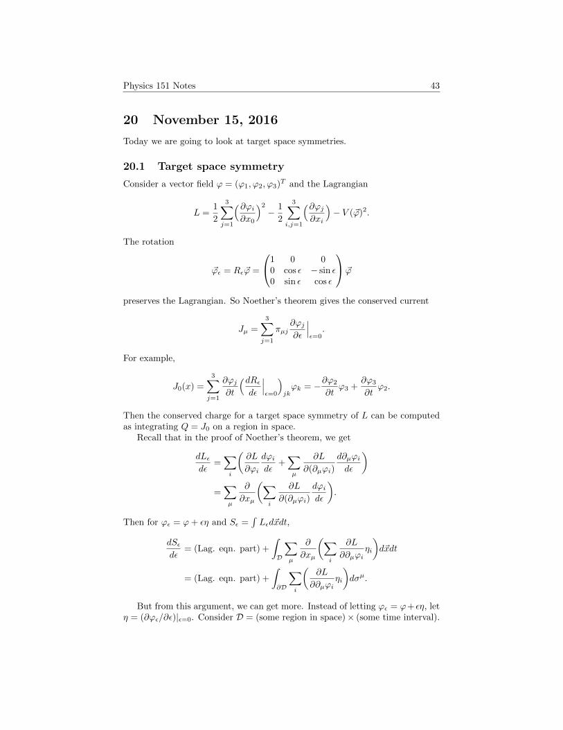
Today we are going to look at target space symmetries.
20.1 Target space symmetry
Consider a vector field ϕ = (ϕ1, ϕ2, ϕ3)T and the Lagrangian
L =1
2
3∑j=1
(∂ϕi∂x0
)2
− 1
2
3∑i,j=1
(∂ϕj∂xi
)− V (~ϕ)2.
The rotation
~ϕε = Rε~ϕ =
1 0 00 cos ε − sin ε0 sin ε cos ε
~ϕ
preserves the Lagrangian. So Noether’s theorem gives the conserved current
Jµ =
3∑j=1
πµj∂ϕj∂ε
∣∣∣ε=0
.
For example,
J0(x) =
3∑j=1
∂ϕj∂t
(dRεdε
∣∣∣ε=0
)jkϕk = −∂ϕ2
∂tϕ3 +
∂ϕ3
∂tϕ2.
Then the conserved charge for a target space symmetry of L can be computedas integrating Q = J0 on a region in space.
Recall that in the proof of Noether’s theorem, we get
dLεdε
=∑i
(∂L
∂ϕi
dϕidε
+∑µ
∂L
∂(∂µϕi)
d∂µϕidε
)=∑µ
∂
∂xµ
(∑i
∂L
∂(∂µϕi)
dϕidε
).
Then for ϕε = ϕ+ εη and Sε =∫Lεd~xdt,
dSεdε
= (Lag. eqn. part) +
∫D
∑µ
∂
∂xµ
(∑i
∂L
∂∂µϕiηi
)d~xdt
= (Lag. eqn. part) +
∫∂D
∑i
(∂L
∂∂µϕiηi
)dσµ.
But from this argument, we can get more. Instead of letting ϕε = ϕ+ εη, letη = (∂ϕε/∂ε)|ε=0. Consider D = (some region in space)× (some time interval).
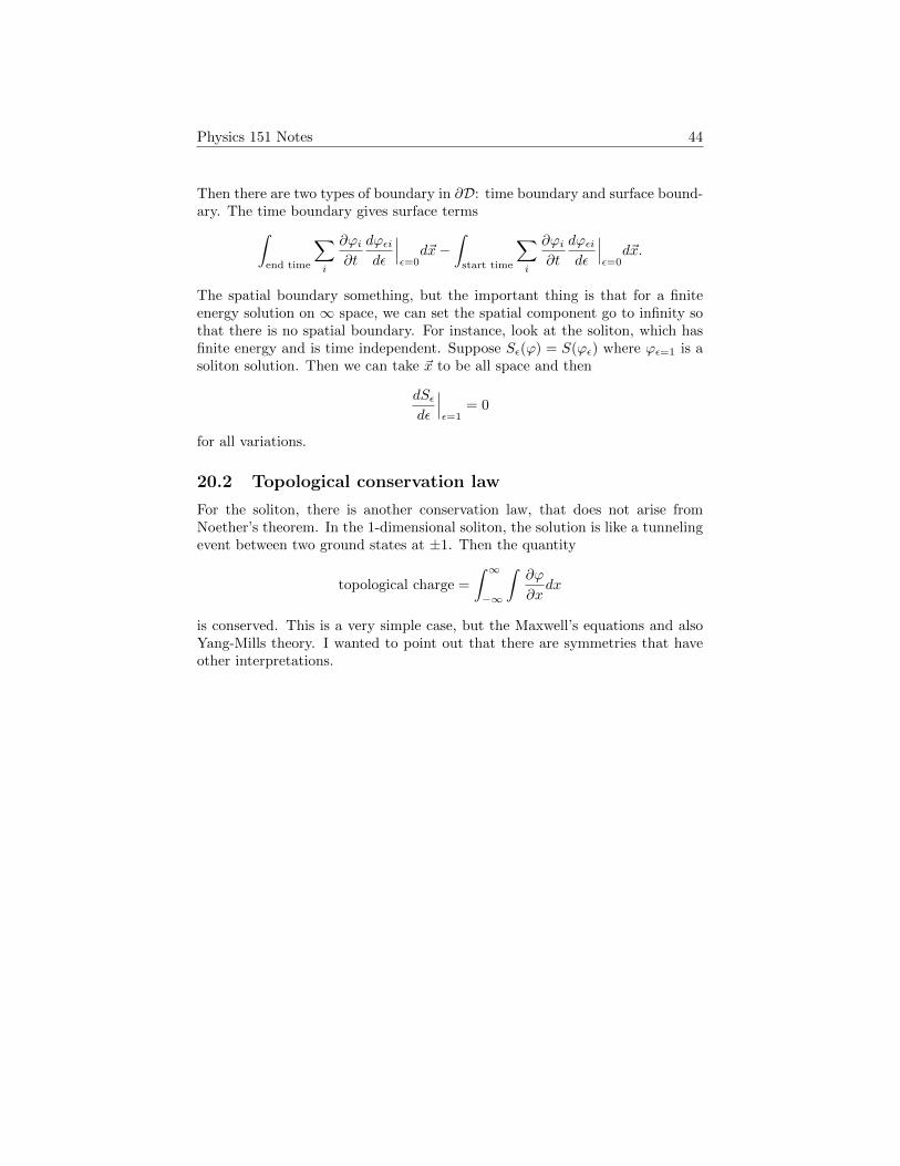
Physics 151 Notes 44
Then there are two types of boundary in ∂D: time boundary and surface bound-ary. The time boundary gives surface terms∫
end time
∑i
∂ϕi∂t
dϕεidε
∣∣∣ε=0
d~x−∫
start time
∑i
∂ϕi∂t
dϕεidε
∣∣∣ε=0
d~x.
The spatial boundary something, but the important thing is that for a finiteenergy solution on ∞ space, we can set the spatial component go to infinity sothat there is no spatial boundary. For instance, look at the soliton, which hasfinite energy and is time independent. Suppose Sε(ϕ) = S(ϕε) where ϕε=1 is asoliton solution. Then we can take ~x to be all space and then
dSεdε
∣∣∣ε=1
= 0
for all variations.
20.2 Topological conservation law
For the soliton, there is another conservation law, that does not arise fromNoether’s theorem. In the 1-dimensional soliton, the solution is like a tunnelingevent between two ground states at ±1. Then the quantity
topological charge =
∫ ∞−∞
∫∂ϕ
∂xdx
is conserved. This is a very simple case, but the Maxwell’s equations and alsoYang-Mills theory. I wanted to point out that there are symmetries that haveother interpretations.
Physics 151 Notes 45
21 November 17, 2016
This class was a review session for the in-class midterm, by the TF.
21.1 Review for the exam—lots of examples
Let us look at the 2-dimensional system
L =1
2(q2
1 − q22)− V (q1, q2); V (q1, q2) = (q2
1 − q22)2.
Then p1 = q1 and p2 = −q2. So the Hamiltonian is given by
H = p1q1 + p2q2 − L =1
2(p2
1 − p22) + V (q1, q2).
Then the transformation(q1(ε)q2(ε)
)=
(cosh ε sinh εsinh ε cosh ε
)(q1
q2
)is a symmetry.
We now apply Noether’s theorem. Because (dq1(ε)/dε)|ε=0 = q2 and (dq2(ε)/dε)|ε=0 =q1, we get
G = p1q2 + q2p1
as the conserved quantity. Let’s compute some Poisson brackets for practice.We have
[q1, G] = q2, [q2, G] = q1, [p1, G] = −p2, [p2, G] = −p1.
Let’s now compute the canonical flow generated by this function. There is a nicetrick to compute this. Recall that such a transformation is canonical. BecauseG is a conserved quantity,
d
dλΞ(λ) = −DGq1(λ) = [q1(λ), G]q,p = [q1(λ), G(λ)]q,p
= [q1(λ), G(λ)]q(λ),p(λ) = q2(λ).
Then
d
dλΞ(λ) =
q2(λ)q1(λ)−p2(λ)−p1(λ)
.
This is a simple differential equation, and so can solve it easily.Let’s now move on and talk about classical field theory. Consider the La-
grangian given by
L =1
2(∂tϕ)2 − 1
2(∂xϕ)2.
Physics 151 Notes 46
The equation of motion will be
∂2t ϕ− ∂2
xϕ = 0.
There is the boost symmetry, but there is also a scaling symmetry given by
ϕε(t, x) = ϕ(εt, εx).
Then
Sε =
∫ε2(
1
2(∂tϕ)2(εt, εx)− (∂xϕ)2(εt, εx)
)dtdx = S.
Physics 151 Notes 47
22 November 29, 2016
Today and Thursday, I am going to talk about the connection between classi-cal mechanics and quantum theory. The first point of view is looking at theSchrodinger equation, given by
i~dψ(t)
dt= Hψ(t).
Another way of looking at this is through the Heisenberg equation, whichlooks like
~d
dtA(t) = i(HA(t)−A(t)H) = i[H,A(t)].
The connection between the two ways were noticed mainly by Dirac. Thesolutions to the two equations are given by
ψ(t) = e−itH/~ψ(0), A(t) = eitH/~A(0)e−itH/~.
Today we are going to concentrate on the Schrodinger picture.
22.1 The Feynman formula
We have the solution to the Schrodinger equation. We can write it as
ψ(t, x) = (e−itHψ)(0, x) =
∫Kt(x, x
′)ψ(0, x′)dx′,
where Kt is the Green’s function.Let us look at the simplest example of the freely moving particle in 1-
dimension. In this case, H = p2/2m. Consider the Fourier transform
ψ(0, x) =1√2π~
∫eipx/~ψ(0, p)dp,
ψ(0, p) =1√2π~
∫e−ipx/~ψ(0, x)dx.
Then the formula for ψ is
ψ(t, x) =1√2π~
∫eipx/~e−
itp2
2m~ ψ(p)dp
=1
2π~
∫ (∫dp eip(x−x
′)/~−i tp2
2m~
)ψ(0, x′)dx′.
So the Green’s function we want is
Kt(x, x′) =
1
2π~
∫ ∞−∞
dp eip(x−x′)/~− itp2
2m~ .
Physics 151 Notes 48
Actually this doesn’t converge, so we have to put a convergence factor and set
Kt(x, x′) = lim
ε→0
1
2π~
∫ ∞−∞
dp eip(x−x′)/~− itp2
2m~ e−εp2
.
If you work it out, then we get the answer
Kt(x, x′) =
√m
2πi~tei
m(x−x′)22~t .
The action of a free particle satisfying the Newton-Lagrange equation isgiven by
Sfree,Newton =m
2
∫ t
0
x2ds =m
2
(x− x′)2
t,
where x is the position at time t and x′ is position at time 0. So we can write
Kt(x, x′) =
√m
2πi~teiSfree,Newton/~.
Now Feynman thought a lot about this equation and tried to see what happensif we take an arbitrary path and average over all paths. And then we would get
Kt(x, x′) =
∫eiSfree(x)/~Dx.
The mathematical problem here is what exactly D(x) is. But you can formulateit, and this was Feynman’s thesis.
Why is it? Note that e−it1H/~e−it2H/~ = e−i(t1+t2)H/~ and so∫Kt1(x, x1)Kt2(x1, x
′)dx1 = Kt1+t2(x, x′).
So if we let x0 = x, and xk be x at time kt/n, then we get
Kt(x, x′) =
∫dx1 · · · dxn−1 Kt/n(x, x1)Kt/n(x1, x2) · · ·Kt/n(xn−1, x
′)
=
(m
2πi~t/n
)n/2 ∫eim2~
tn
∑n−1j=0
(xj−xj+1)2
(t−n)2 dx1 · · · dxn−1
≈(
m
2πi~t/n
)n/2 ∫ei
m2~
∫ t0x2dsdx1 · · · dxn−1.
Here we get a constant, that tends to infinity as n→∞, and some dx1 · · · dxn−1,that also doesn’t make sense as n → ∞. But at least in some sense, we havethe formula
Kt(x, x′) ≈
∫eiSfree/~Dx.
Physics 151 Notes 49
This is the Feynman formula.What if you have a particle that is not free? The answer is that you can
just replace Sfree by a general S. This is actually the same as first letting theparticle move freely for one time increment, then giving a jolt by the potential,then letting the particle move freely again, giving a second jolt, and alternatingthis process. So if H = Hfree = V , then
limn→∞
(eA/neB/n)n = eA+B .
This is why we can simply replace the free action with the general action.
Physics 151 Notes 50
23 December 1, 2016
Last time we looked at the Schrodinger equtation and got
Kt(x, x′) =
∫eiS(x(t))/~Dx.
In the case of the free particle, we further had
Kt(x, x′) =
∫eiS(x(t))/~Dx = eiSclassical/~.
23.1 The Heisenberg equation
The Heisenberg equation is given by
eitH/~Ae−itH/~ = A(t)
for an observable A.There is a connection between this equation and the Poisson brackets we
saw in classical mechanics. Recall that
[xi, pj ]ξ =∑k
( ∂xi∂xk
∂pi∂pk− ∂xi∂pk
∂pj∂xk
)= δij .
In quantum theory, we have the relation (where we put the hat to distinguishfrom the classical counterpart)
[xi, pj ] = xipj − pj xi = xi
(~i
∂
∂xj
)−(~i
∂
∂xj
)xi =
~iδij .
So in some sense, [xi, pj ] = [xi, pj ]ξi~. This suggests the classical limit identityis given by
lim~→0
1
i~[A, B] = [A,B]ξ.
Given a function A, in classical mechanics, we get a flow
e−λDAB = B − λ[A,B]ξ +λ2
2[A, [A,B]ξ]ξ + · · · .
This corresponds to the unitary operator eiλA/~ in quantum mechanics. If we
expand eiλA/~Be−iλA/~, we get
eiλA/~Be−iλA/~ = f(λ) =
N∑k=0
f (k)(0)λk
k!+O(λN+1)
= B +iλ
~[A, B] +
( iλ~
)2 1
2[A, [A, B]] + · · · .
Physics 151 Notes 51
So as ~→ 0, this goes to
B − λ[A,B]ξ +λ2
2[A, [A,B]ξ]ξ + · · · .
In the classical setting, e−λDA is a canonical transformation, and in the quantum
setting, eiλA/~ is a unitary transformation.We also had another important set of Poisson brackets, which are the ones
between the angular momenta. Continuing the analogue, we have
[Li, Lj ] = i~∑k
εijkLk, [Li, Lj ]ξ =∑k
εijkLk.
Still, we cannot talk about it in more generality. For instance, recall thatx1p1 in classical mechanics generated the scale transformation. But here we
run into an ambiguity. Is the right analogue x1p1 or p1x1? If eiλA/~ is to be aunitary operator, the operator A has to be hermitian. But the adjoint of x1p1
is p1x1 and vice versa. So what we do is to take
xp → 1
2(xp+ px).
Let me show you something more disturbing. What about A = px3? WillA = 1
2 (px3 + x3p) do? Let us compute the eigenvalues of A. If you solve the
equation Aψ(x) = λψ(x), you get
ψ(x) = c1
x3/2e−iλ2x2
.
This is square-integrable if and only if λ is in the lower half plane. So every λ inthe lower half plane is an eigenvalue of A! This is because A is not self-adjoint.
Index
action, 17
canonical transformation, 29contravariant vector, 11covariant vector, 10, 12
directional derivative, 17
energy-momentum density, 39
Feynman formula, 49
Hamilton’s equations, 25Hamiltonian, 21Heisenberg equation, 47, 50holomonic constraints, 16
Kepler’s laws, 6
Lagrange equations, 37Lagrangian, 10Lenz vector, 5Lie derivative, 29
Noether’s theorem, 22, 24
phase space, 26Poisson bracket, 29
relativistic particle, 21
Schrodinger equation, 47symmetry, 35
topological conservation, 44
vectorin phase space, 33
52