Physics 42200

Waves & Oscillations

Spring 2016 SemesterMatthew Jones

Lecture 23 – Review

Midterm Exam:

Date: Thursday, March 10th

Time: 8:00 – 10:00 pm

Room: MSEE B012

Material: French, chapters 1-8

You can bring one double sided page

of notes, formulas, examples, etc.

Review

1. Simple harmonic motion (one degree of freedom)

– mass/spring, pendulum, floating objects, RLC circuits

– damped harmonic motion

2. Forced harmonic oscillators

– amplitude/phase of steady state oscillations

– transient phenomena

3. Coupled harmonic oscillators

– masses/springs, coupled pendula, RLC circuits

– forced oscillations

4. Uniformly distributed discrete systems

– masses on string fixed at both ends

– lots of masses/springs

Review

5. Continuously distributed systems (standing waves)

– string fixed at both ends

– sound waves in pipes (open end/closed end)

– transmission lines

– Fourier analysis

6. Progressive waves in continuous systems

– reflection/transmission coefficients

Simple Harmonic Motion

• Any system in which the force is opposite the displacement will oscillate about a point of stable equilibrium

• If the force is proportional to the displacement it will undergo simple harmonic motion

• Examples:

– Mass/massless spring

– Elastic rod (characterized by Young’s modulus)

– Floating objects

– Torsion pendulum (shear modulus)

– Simple pendulum

– Physical pendulum

– LC circuit

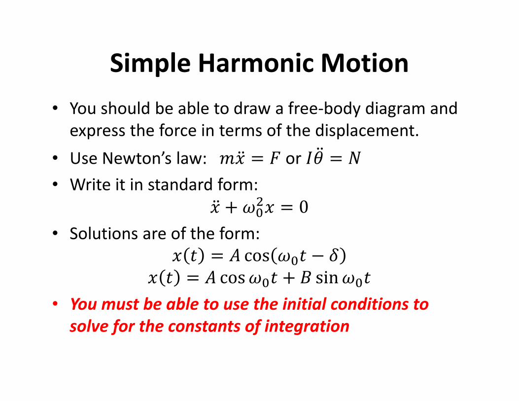
Simple Harmonic Motion

• You should be able to draw a free-body diagram and

express the force in terms of the displacement.

• Use Newton’s law: ��� = � or ��� = �• Write it in standard form:

�� + ��� = 0• Solutions are of the form:

� � = � cos �� − �� � = � cos�� + � sin��

• You must be able to use the initial conditions to

solve for the constants of integration

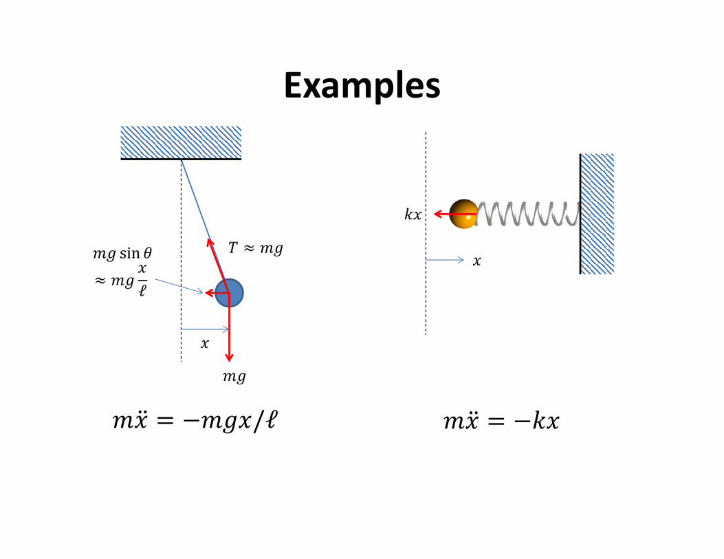
Examples

�

� ≈ ��

��

�� sin �≈ �� �ℓ

��� = −���/ℓ

�

��

��� = −��

Examples

�

��� =?

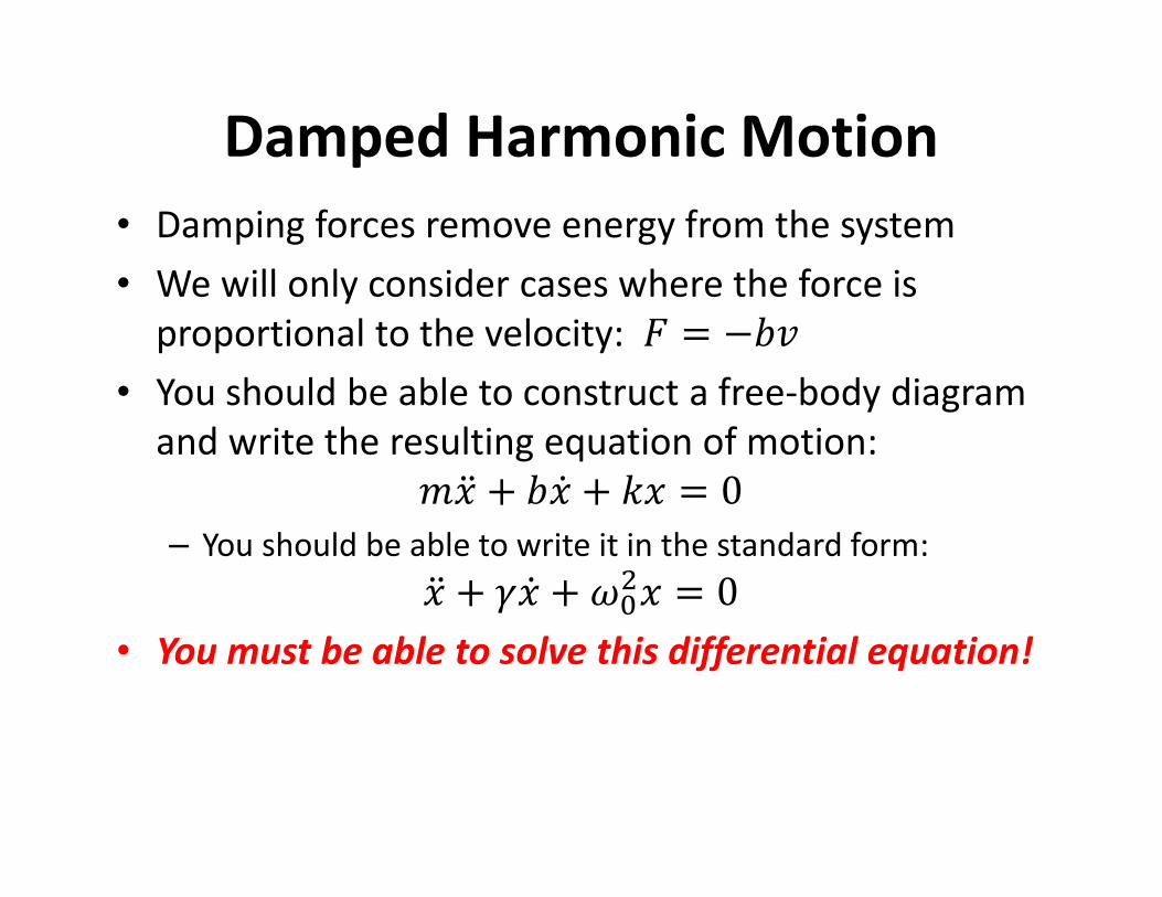
Damped Harmonic Motion

• Damping forces remove energy from the system

• We will only consider cases where the force is

proportional to the velocity: � = − !• You should be able to construct a free-body diagram

and write the resulting equation of motion:

��� + �" + �� = 0– You should be able to write it in the standard form:

�� + #�" + ��� = 0• You must be able to solve this differential equation!

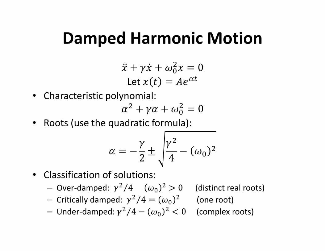
Damped Harmonic Motion

�� + #�" + ��� = 0Let � � = �$%&

• Characteristic polynomial:

'� + #' + �� = 0• Roots (use the quadratic formula):

' = −#2 ±

#�4 − � �

• Classification of solutions:

– Over-damped: #� 4⁄ − � � > 0 (distinct real roots)

– Critically damped: #� 4⁄ = � � (one root)

– Under-damped: #� 4⁄ − � � < 0 (complex roots)

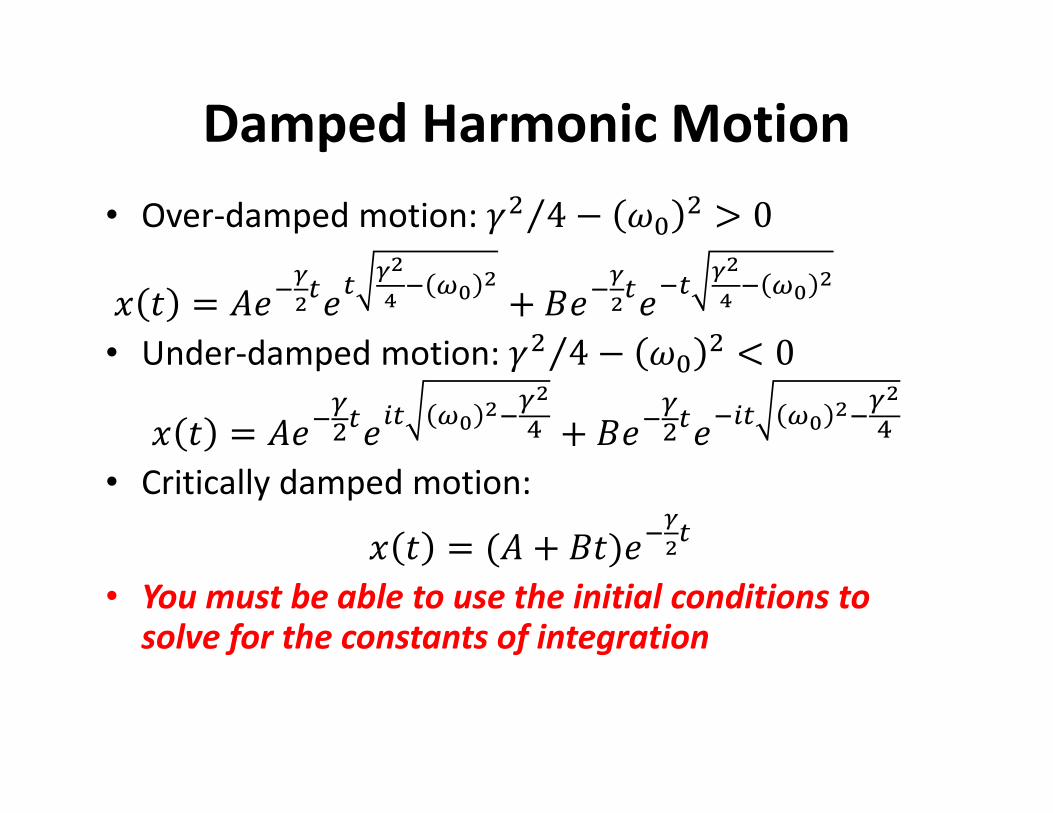
Damped Harmonic Motion

• Over-damped motion: #� 4⁄ − � � > 0� � = �$./

0&$& /01 . 23 0 + �$./

0&$.& /01 . 23 0

• Under-damped motion: #� 4⁄ − � � < 0� � = �$.4�&$5& 23 0.406 + �$.4�&$.5& 23 0.406

• Critically damped motion:

� � = (� + ��)$./0&

• You must be able to use the initial conditions to

solve for the constants of integration

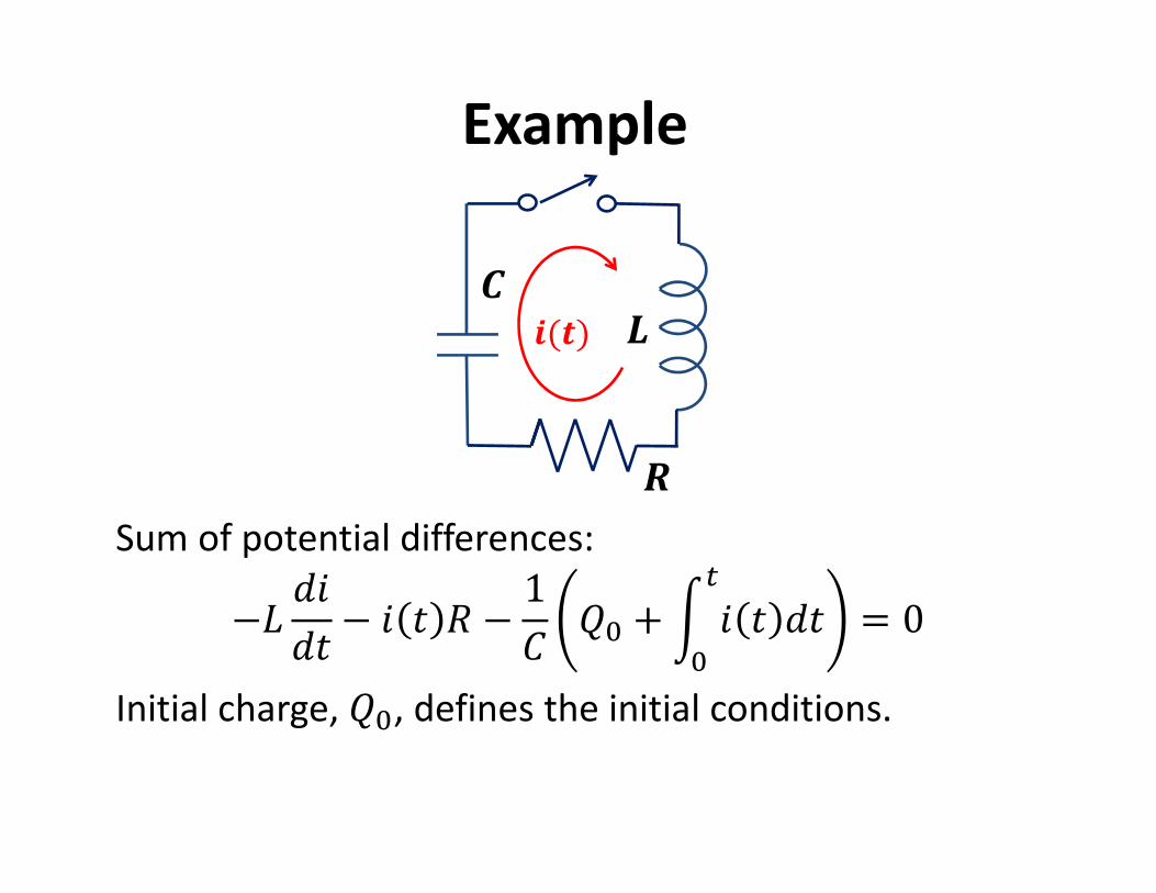
Example

Sum of potential differences:

−9 :;:� − ; � < − 1> ?� +@ ; � :�

&

�= 0

Initial charge, ?�, defines the initial conditions.

AB(C) D

E

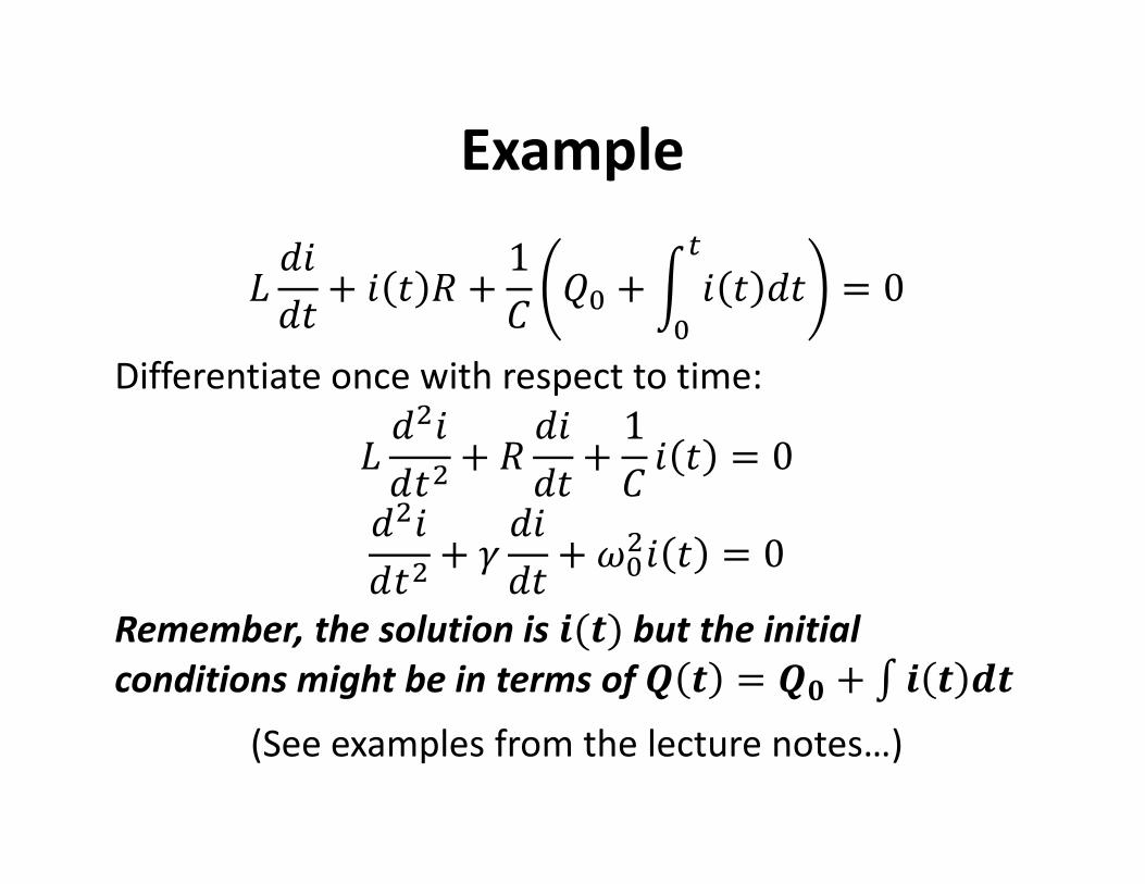
Example

9 :;:� + ; � < + 1> ?� +@ ; � :�

&

�= 0

Differentiate once with respect to time:

9 :�;

:�� + < :;:� +

1> ; � = 0

:�;:�� + # :;:� + ��; � = 0

Remember, the solution is B(C) but the initial

conditions might be in terms of F C = FG + H B C IC(See examples from the lecture notes…)

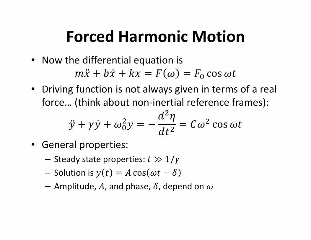
Forced Harmonic Motion

• Now the differential equation is

��� + �" + �� = � = �� cos�• Driving function is not always given in terms of a real

force… (think about non-inertial reference frames):

J� + #J" + ��J = −:�K:�� = >� cos�

• General properties:

– Steady state properties: � ≫ 1/#– Solution is J � = � cos � − �– Amplitude, �, and phase, �, depend on

Forced Harmonic Motion

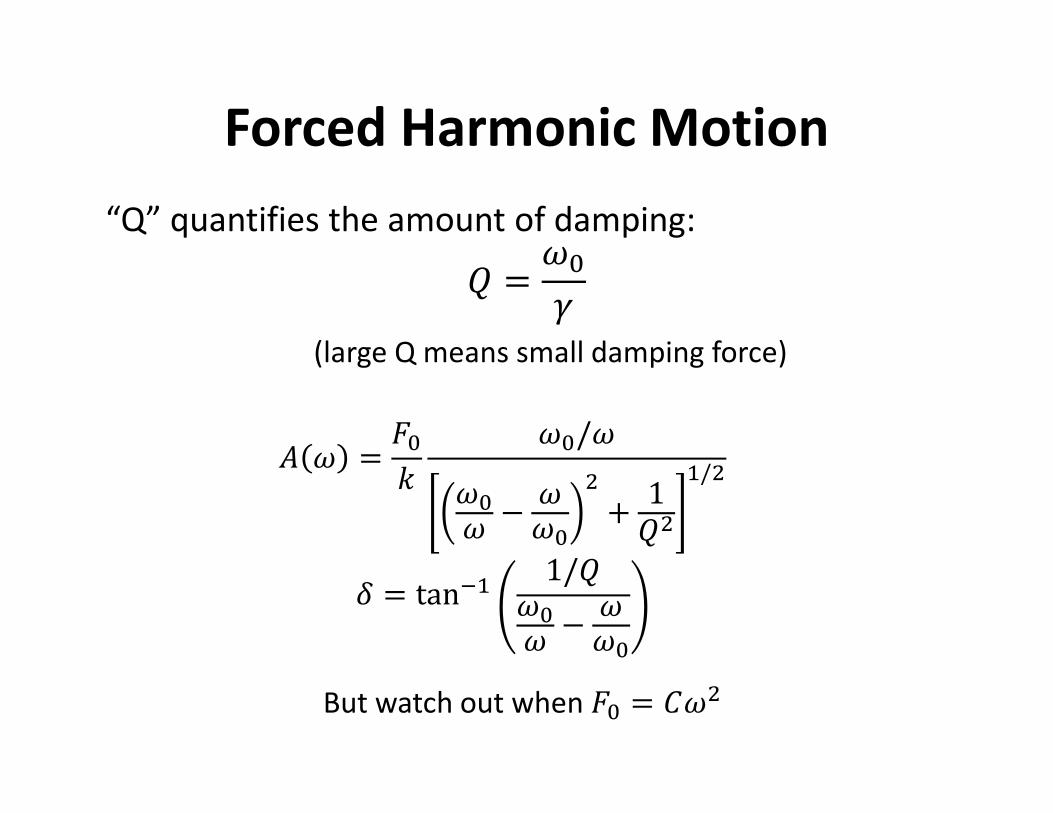
“Q” quantifies the amount of damping:

? = �#

(large Q means small damping force)

� = ���

�/� −

�� + 1

?�M/�

� = tan.M 1/?� −

�But watch out when �� = >�

Resonance

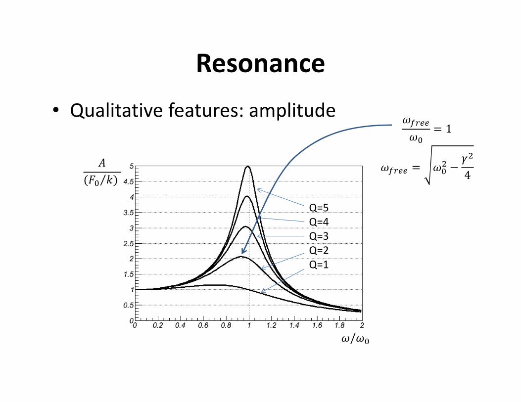
• Qualitative features: amplitude

/�

�(�� �⁄ )

Q=5

Q=4

Q=3

Q=2

Q=1

PQRR�

= 1

PQRR = �� − #�4

/�

ST()�� ��/2� ? = 10

? = 5

? = 3

? = 1

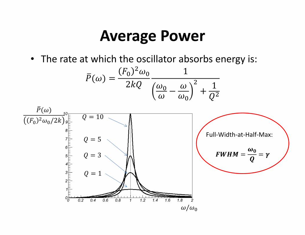
Average Power

• The rate at which the oscillator absorbs energy is:

ST() = �� ��2�?

1

�−�

�

+1

?�

Full-Width-at-Half-Max:

WXYZ =[G

F= \

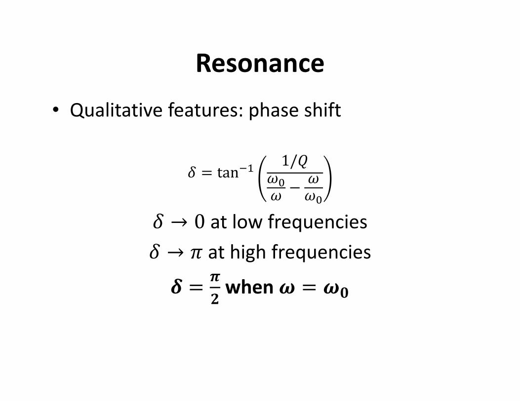
Resonance

• Qualitative features: phase shift

� = tan.M 1/?� −

�� → 0 at low frequencies

� → ^ at high frequencies

_ = `a when [ = [G

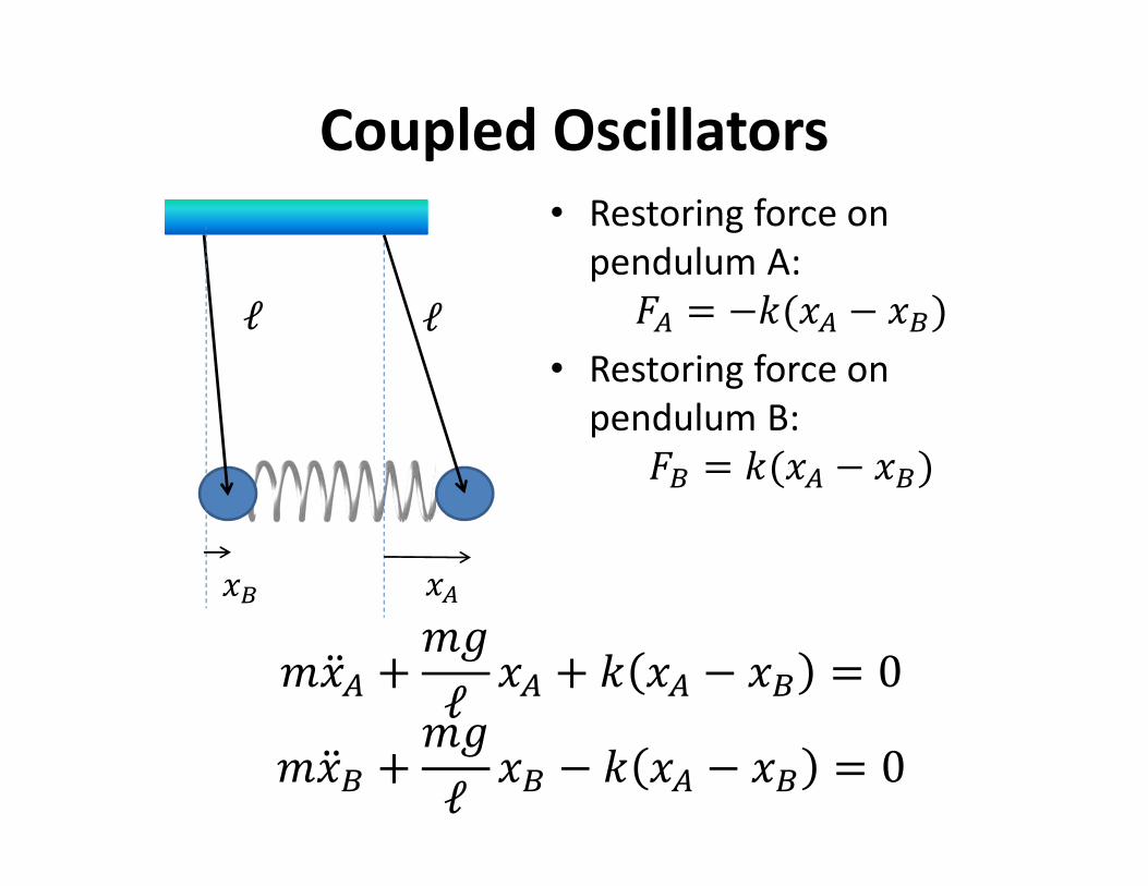
Coupled Oscillators

• Restoring force on

pendulum A:

�b = −�(�b − �c)• Restoring force on

pendulum B:

�c = �(�b − �c)

ℓ

�c �b

ℓ

���b +��ℓ �b + � �b − �c = 0

���c +��ℓ �c − � �b − �c = 0

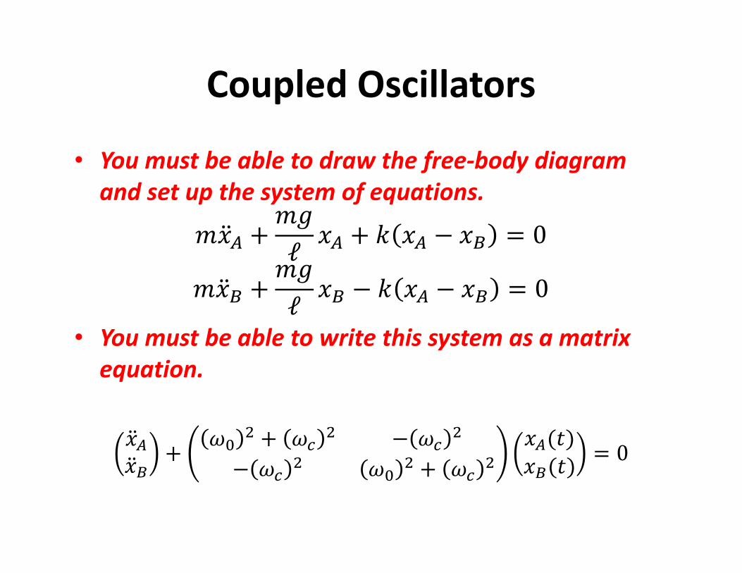
Coupled Oscillators

• You must be able to draw the free-body diagram

and set up the system of equations.

���b +��ℓ �b + � �b − �c = 0

���c +��ℓ �c − � �b − �c = 0

• You must be able to write this system as a matrix

equation.

��b��c + � � + d � − d �− d � � � + d �

�b(�)�c(�) = 0

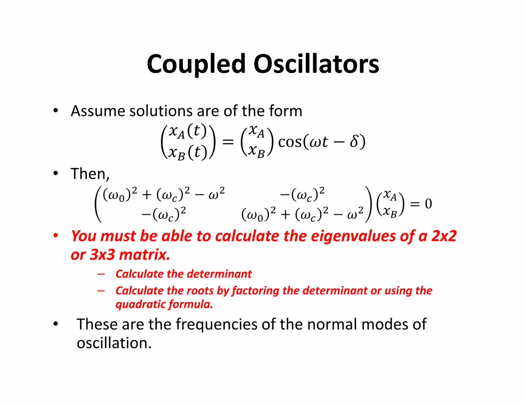
Coupled Oscillators

• Assume solutions are of the form�b(�)�c(�) = �b�c cos � − �

• Then,

� � + d � −� − d �− d � � � + d � −�

�b�c = 0• You must be able to calculate the eigenvalues of a 2x2

or 3x3 matrix.– Calculate the determinant

– Calculate the roots by factoring the determinant or using the

quadratic formula.

• These are the frequencies of the normal modes of oscillation.

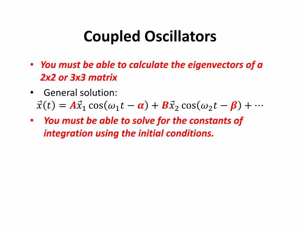
Coupled Oscillators

• You must be able to calculate the eigenvectors of a

2x2 or 3x3 matrix

• General solution:

�e � = f�eM cos M� − g + h�e� cos �� − i +⋯• You must be able to solve for the constants of

integration using the initial conditions.

Coupled Discrete Systems• The general method of calculating eigenvalues will always

work, but for simple systems you should be able to decouple

the equations by a change of variables.

ℓ

�c �b

ℓ���b +��

ℓ �b + � �b − �c = 0���c +��

ℓ �c − � �b − �c = 0��b + � � + d � �b − d ��c = 0��c + � � + d � �c − d ��b = 0

� = �/ℓ, d = �/�kM = �b + �ck� = �b − �ck�M + � �kM = 0

k�� + ′ �k� = 0

1

4

3

2

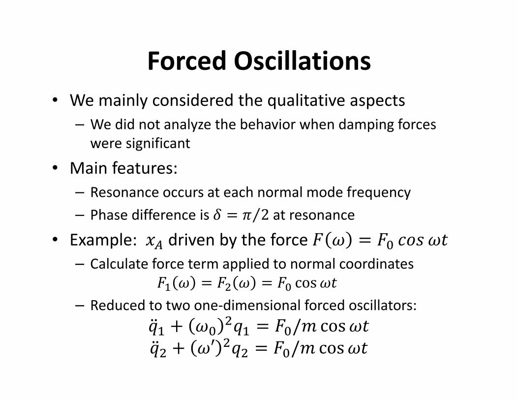
Forced Oscillations

• We mainly considered the qualitative aspects

– We did not analyze the behavior when damping forces

were significant

• Main features:

– Resonance occurs at each normal mode frequency

– Phase difference is � = ^ 2⁄ at resonance

• Example: �b driven by the force � = �� mno �– Calculate force term applied to normal coordinates

�M = �� = �� cos�– Reduced to two one-dimensional forced oscillators:

k�M + � �kM = ��/� cos�k�� + ′ �k� = ��/� cos�

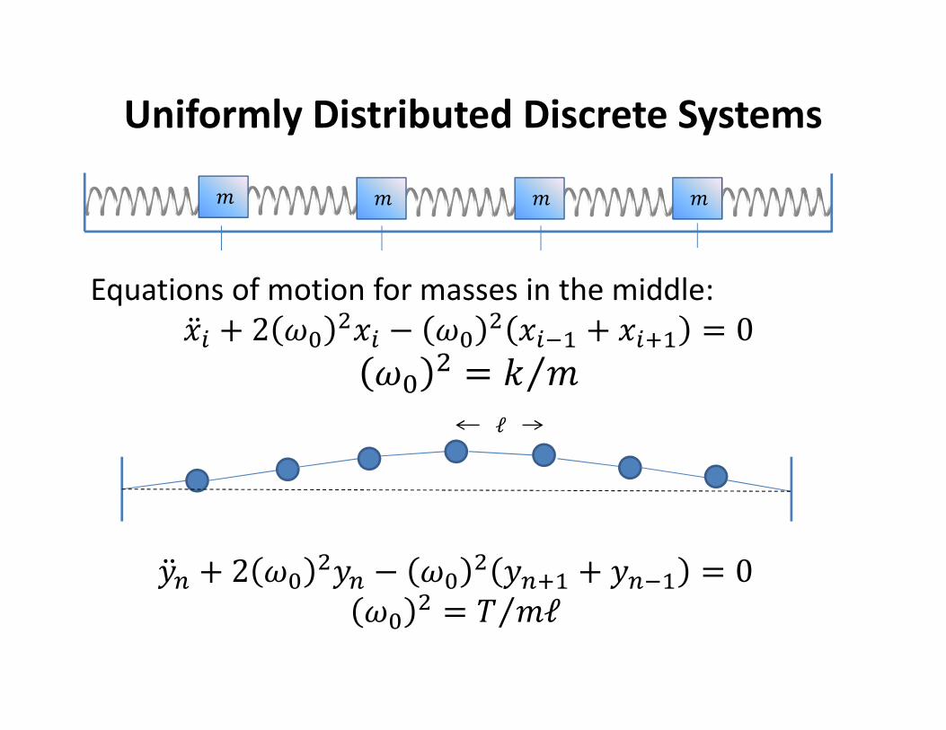
Equations of motion for masses in the middle:

��5 + 2 � ��5 − � � �5.M + �5pM = 0� � = � �⁄

� � � �

Uniformly Distributed Discrete Systems

ℓ

J�q + 2 � �Jq − � � JqpM + Jq.M = 0� � = � �ℓ⁄

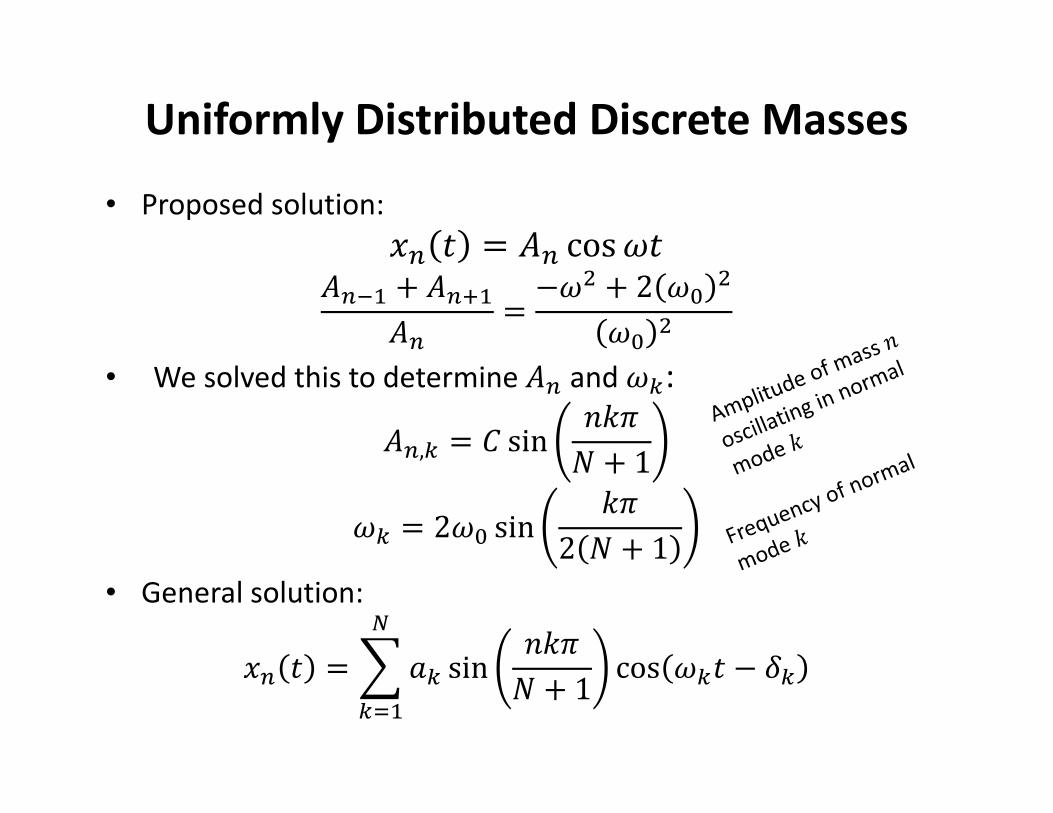
• Proposed solution:

�q � = �q cos��q.M + �qpM�q

= −� + 2 � �� �

• We solved this to determine �q and r:

�q,r = > sin t�^� + 1

r = 2� sin �^2 � + 1

• General solution:

�q � = uvr sin t�^� + 1

w

rxMcos r� − �r

Uniformly Distributed Discrete Masses

• General solution for mass t:

�q � = uvr sin t�^� + 1

w

rxMcos r� − �r

• Orthogonality relation:

usin ��^� + 1 sin t�^

� + 1w

rxM= �

2 �yq

• Solution to initial value problem:

u�q 0w

qxMsin t�^

� + 1 = �2 vr mno �r

Vibrations of Continuous Systems

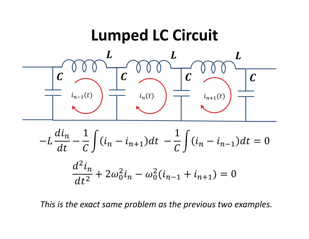
Lumped LC Circuit

−9 :;q:� − 1> @ ;q − ;qpM :� − 1

> @ ;q − ;q.M :� = 0:�;q:�� + 2��;q −��(;q.M + ;qpM) = 0

AD

AD

AD

A;q(�) ;qpM(�);q.M(�)

This is the exact same problem as the previous two examples.

Forced Coupled Oscillators

• Qualitative features are the same:

– Motion can be decoupled into a set of �independent oscillator equations (normal modes)

– Amplitude of normal mode oscillations are large

when driven with the frequency of the normal

mode

– Phase difference approaches ^/2 at resonance

• You should be able to anticipate the

qualitative behavior when coupled oscillators

are driven by a periodic force.

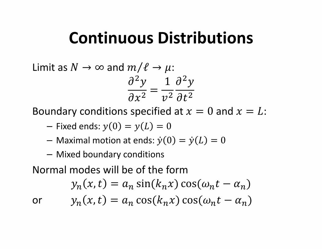
Continuous Distributions

Limit as � → ∞ and � ℓ⁄ → {:

|�J|�� =

1!�

|�J|��

Boundary conditions specified at � = 0 and � = 9:

– Fixed ends: J 0 = J 9 = 0– Maximal motion at ends: J" 0 = J" 9 = 0– Mixed boundary conditions

Normal modes will be of the form

Jq �, � = vq sin(�q�) cos(q� − 'q)or Jq �, � = vq cos(�q�) cos(q� − 'q)

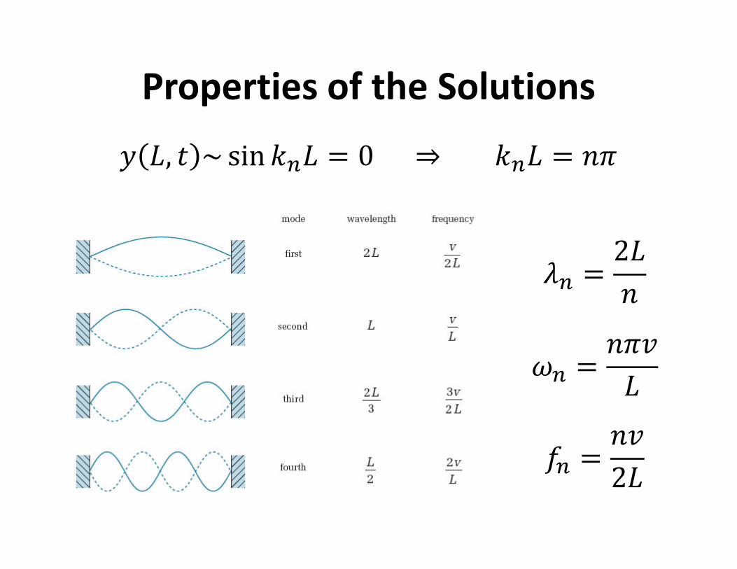
Properties of the Solutions

J 9, � ~ sin �q9 = 0 ⇒ �q9 = t^

�q = 29

t

q =t^!

9

�q =t!

29

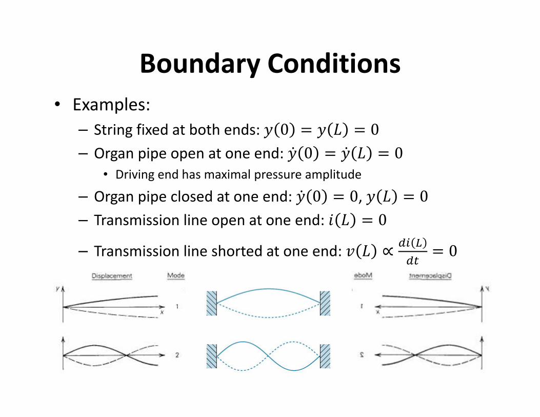
Boundary Conditions

• Examples:

– String fixed at both ends: J 0 = J 9 = 0– Organ pipe open at one end: J" 0 = J" 9 = 0

• Driving end has maximal pressure amplitude

– Organ pipe closed at one end: J" 0 = 0, J 9 = 0– Transmission line open at one end: ; 9 = 0– Transmission line shorted at one end: ! 9 ∝ �5 �

�& = 0

Fourier Analysis

• Normal modes satisfying J 0 = J 9 = 0:Jq �, � = vq sin t^�

9 cos q� − 'q• General solution:

J �, � = uvq sin t^�9 cos q� − 'q

�

qxM• Initial conditions:

J �, 0 = uvq sin t^�9 cos 'q

�

qxM= uv′q sin t^�

9�

qxM

J" �, 0 = −uvqq sin t^�9 sin 'q

�

qxM= u ′q sin t^�

9�

qxM

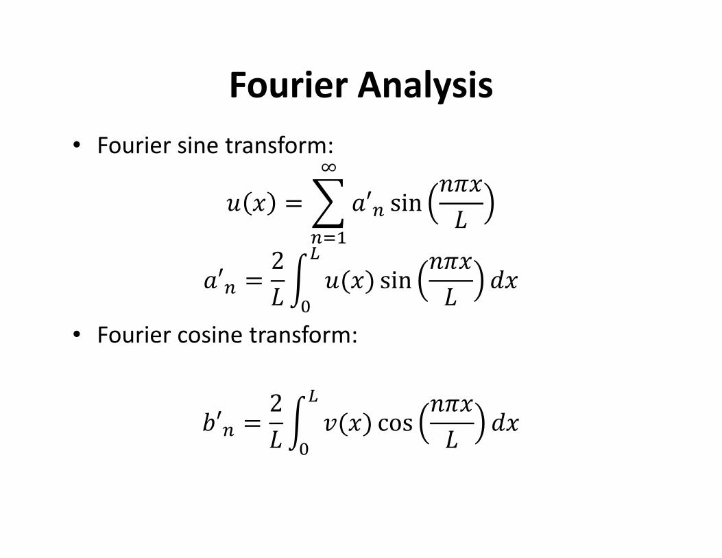
Fourier Analysis

• Fourier sine transform:

� � = uv′q sin t^�9

�

qxMv′q = 2

9@ �(�) sin t^�9 :�

�

�• Fourier cosine transform:

′q = 29@ !(�) cos t^�

9 :��

�

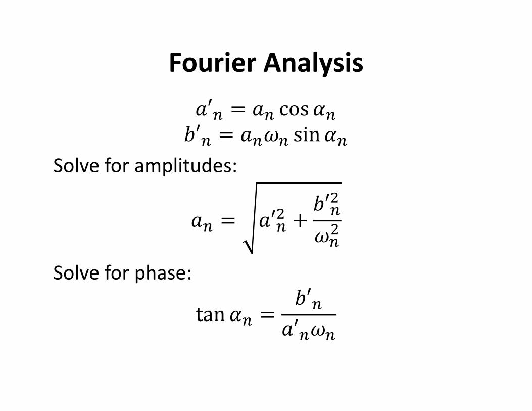
Fourier Analysis

v′q = vq cos 'q ′q = vqq sin 'qSolve for amplitudes:

vq = v′q� + ′q�q�

Solve for phase:

tan 'q = ′qv′qq

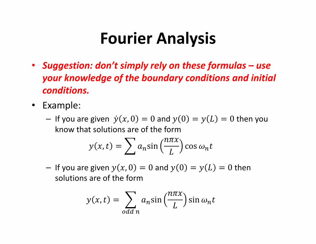
Fourier Analysis

• Suggestion: don’t simply rely on these formulas – use

your knowledge of the boundary conditions and initial

conditions.

• Example:

– If you are given J" �, 0 = 0 and J 0 = J 9 = 0 then you

know that solutions are of the form

J �, � = uvqsin t^�9 cosq�

– If you are given J �, 0 = 0 and J 0 = J 9 = 0 then

solutions are of the form

J �, � = u vqsin t^�9 sinq�

���q

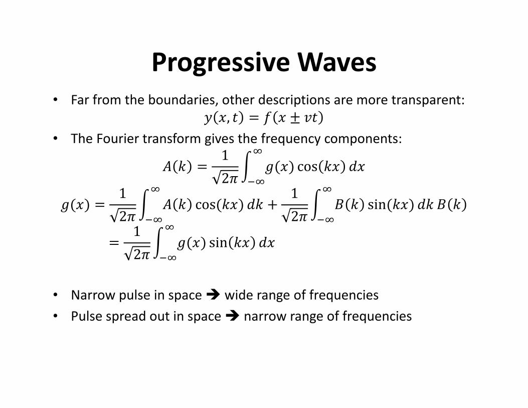
Progressive Waves

• Far from the boundaries, other descriptions are more transparent:

J �, � = � � ± !�• The Fourier transform gives the frequency components:

� � = 12^@ �(�) cos �� :�

�

.��(�) = 1

2^@ � � cos(��) :��

.�+ 1

2^@ � � sin(��) :��

.�� �

= 12^@ �(�) sin �� :�

�

.�

• Narrow pulse in space � wide range of frequencies

• Pulse spread out in space � narrow range of frequencies

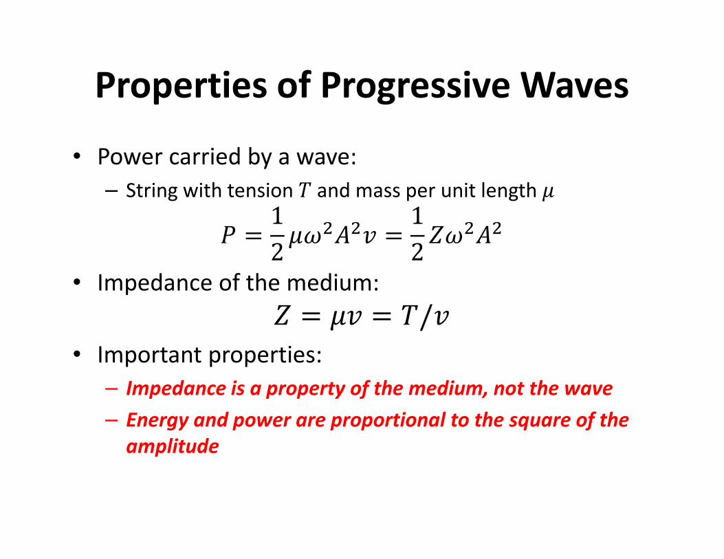
Properties of Progressive Waves

• Power carried by a wave:

– String with tension � and mass per unit length {S = 1

2{���! = 12����

• Impedance of the medium:

� = {! = �/!• Important properties:

– Impedance is a property of the medium, not the wave

– Energy and power are proportional to the square of the

amplitude

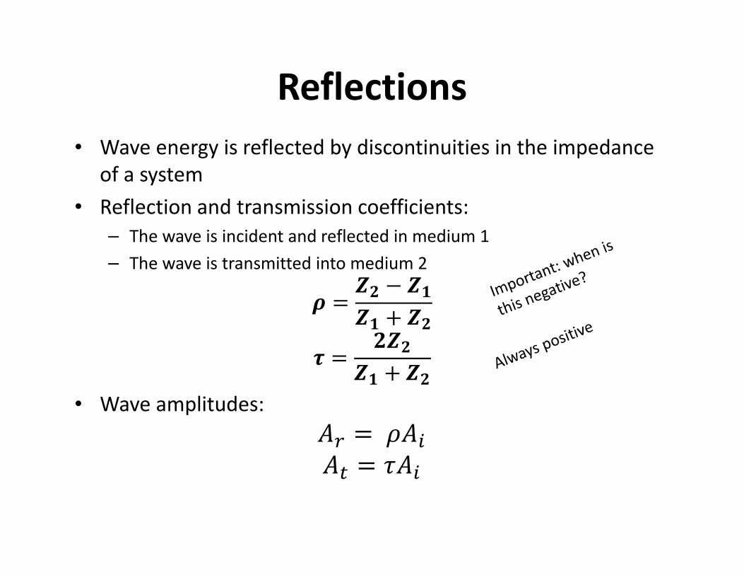
Reflections

• Wave energy is reflected by discontinuities in the impedance

of a system

• Reflection and transmission coefficients:

– The wave is incident and reflected in medium 1

– The wave is transmitted into medium 2

� = �a − ���� + �a

� = a�a�� + �a

• Wave amplitudes:

�Q = ��5�& = ��5

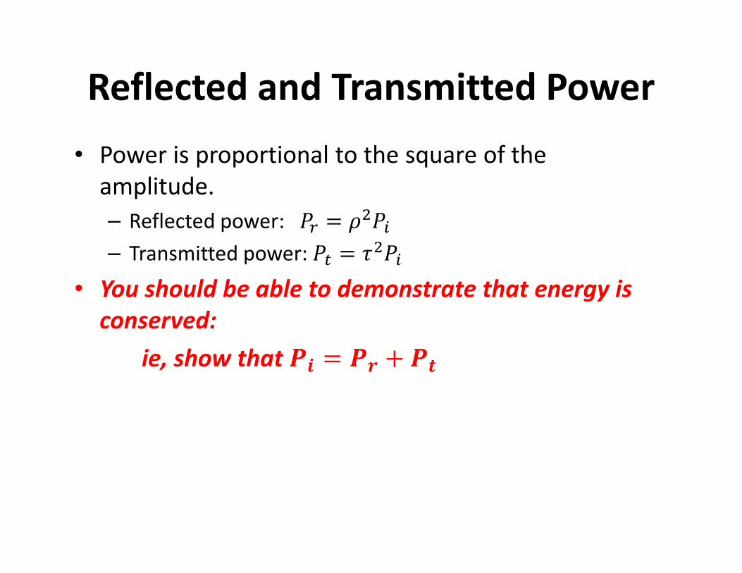
Reflected and Transmitted Power

• Power is proportional to the square of the

amplitude.

– Reflected power: SQ = ��S5– Transmitted power: S& = ��S5

• You should be able to demonstrate that energy is

conserved:

ie, show that �B = �� + �C

That’s all for now…

• Study these topics – make sure you

understand the examples and assignment

questions.

• Midterm exams from previous years are also

available on the web.

• Next topics: waves applied to optics.