Embed Size (px)
Citation preview
The Pennsylvania State University
The Graduate School
Department of Civil and Environmental Engineering
PHYSICS BASED, INTEGRATED MODELING OF
HYDROLOGY AND HYDRAULICS AT WATERSHED SCALES
A Thesis in
Civil Engineering
by
Guobiao Huang
2006 Guobiao Huang
Submitted in Partial Fulfillment
of the Requirements
for the Degree of
Doctor of Philosophy
August 2006

The thesis of Guobiao Huang was reviewed and approved* by the following:
Gour-Tsyh (George) Yeh
Provost Professor of Civil Engineering
Thesis Co-Advisor
Co-Chair of Committee
Arthur C. Miller
Distinguished Professor of Civil Engineering
Thesis Co-Advisor
Co-Chair of Committee
Christopher J. Duffy
Professor of Civil Engineering
Derek Elsworth
Professor of Geo-Environmental Engineering
Peggy A. Johnson
Professor of Civil Engineering
Head of the Department of Civil and Environmental Engineering
*Signatures are on file in the Graduate School
iii
ABSTRACT
This thesis presents the major findings in the development of the hydrology and
hydraulics modules of a first principle, physics-based watershed model (WASH123D
Version 1.5). The numerical model simulates water movement in watersheds with
individual water flow components of one-dimensional stream/channel network flow, two-
dimensional overland flow and three-dimensional variably saturated subsurface flow and
their interactions.
Firstly, the complete Saint Venant equations/2-D shallow water equations
(dynamic wave equations) and the kinematic wave or diffusion wave approximations
were implemented as three solution options for 1-D channel network and 2-D overland
flow. Different solution techniques are considered for the governing equations based on
physical reasoning and their mathematical property. A characteristic based finite element
method is chosen for the hyperbolic-type dynamic wave model. And the Galerkin finite
element method is used to solve the diffusion wave model. Careful choice of numerical
methods is needed even for the simple kinematic wave model. Since the kinematic wave
equation is of pure advection, the backward method of characteristics is used for
kinematic wave model. Diffusion wave and kinematic wave approximations are found in
many surface runoff routing models. The error in these models has been characterized for
some cases of overland flow over simple geometry. However, the nature and propagation
of these approximation errors under more complex 2-D flow conditions are not well
known. These issues are evaluated within WASH123D with comparison of simulation
iv
results of several example problems. The accuracy of the three wave models for 1-D
channel flow was evaluated with several non-trivial (trans-critical flow; varied bottom
slopes with frictions and non-prismatic cross-section) benchmark problems (MacDonnell
et al., 1997). The test examples for 2-D overland flow include: (1) a simple rainfall-
runoff process on a single plane with constant rainfall excess that has a kinematic
analytical solution under steep slope condition. A range of bottom slopes (mild, average
and steep slope) are numerically solved with the three wave models and compared; (2)
Iwagaki (1955) overland flow experiments on a cascade of three planes with shock
waves; (3) overland flow in a hypothetical wetland. The applicability of dynamic-wave,
diffusion-wave and kinematic-wave models to real watershed modeling is discussed with
simulation results from these numerical experiments. It was concluded that kinematic
wave model could lead to significant errors in most applications. On the other hand,
diffusion wave model is adequate for modeling overland flow in most natural watersheds.
The complete dynamic wave equations are required in low-terrain areas such as flood
plains or wetlands and many transient fast flow situations.
Secondly, issues about the coupling between surface water and subsurface flow
are investigated. In the core of an integrated watershed model is the coupling among
surface water and subsurface water flows. Recently, there is a tendency of claiming the
fully coupled approach for surface water and groundwater interactions in the hydrology
literature. One example is the assumption of a gradient type flux equation based on
Darcy’s Law (linkage term) and the numerical solution of all governing equations in a
single global matrix. We argue that this is only a special case of all possible coupling
v
combinations and if not applied with caution, the non-physical interface parameter
becomes a calibration tool. Generally, there are two cases based on physical nature of
the interface: continuous or discontinuous assumption, when a sediment layer exists at
the interface, the discontinuous assumption may be justified. As for numerical schemes,
there are three cases: time-lagged, iterative and simultaneous solutions. Since modelers
often resort to the simplest, fastest schemes in practical applications, it is desirable to
quantify the potential error and performance of different coupling schemes. We evaluate
these coupling schemes in a finite element watershed model, WASH123D. Numerical
experiments are used to compare the performance of each coupling approach for different
types of surface water and groundwater interactions. These are in terms of surface water
and subsurface water solutions and exchange fluxes (e.g. infiltration/seepage rate). It is
concluded that different coupling approaches are justified for flow problems of different
spatial and temporal scales and the physical setting of the interface.
Thirdly, The Method of Characteristics (MOC) in the context of finite element
method was applied to the complete 2-D shallow water equations for 2-D overland flow.
For two-dimensional overland flow, finite element or finite volume methods are more
flexible in dealing with complex boundary. Recently, finite volume methods have been
very popular in numerical solution of the shallow water equations. Some have pointed out
that finite volume methods for 2-D flow are fundamentally one-dimensional (normal to
the cell interface). The results may rely on the grid orientation. The search for genuinely
multidimensional numerical schemes for 2-D flow is an active topic. We consider the
Method of Characteristics (MOC) in the context of finite element method as a good
vi
alternative. Many researchers have pointed out the advantage of MOC in solving 2-D
shallow water equations that are of the hyperbolic type that has wave-like solutions and at
the same time, considered MOC for 2-D overland flow being non-tractable on complex
topography. The intrinsic difficulty in implementing MOC for 2-D overland flow is that
there are infinite numbers of wave characteristics in the 2-D context, although only three
independent wave directions are needed for a well-posed solution to the characteristic
equations. We have implemented a numerical scheme that attempts to diagonalize the
characteristic equations based on pressure and velocity gradient relationship. This new
scheme was evaluated by comparison with other choice of wave characteristic directions
in the literature. Example problems of mixed sub-critical flow/super-critical flow in a
channel with approximate analytical solution was used to verify the numerical algorithm.
Then experiments of overland flow on a cascade of three planes (Iwagaki 1955) were
solved by the new method. The circular dam break problem was solved with different
selections of wave characteristic directions and the performance of each selection was
evaluated based on accuracy and numerical stability. Finally, 2-D overland flow over
complex topography in a wetland setting with very mild slope was solved by the new
numerical method to demonstrate its applicability.
Finally, the physics-based, integrated watershed model was tested and validated
with the hydrologic simulation of a pilot constructed wetland in South Florida. For this
field problem strong surface water and groundwater interactions are a key component of
the hydrologic processes. The site has extensive field measurement and monitoring that
provide point scale and distributed data on surface water levels, groundwater levels and
vii
physical range of hydraulic parameters and hydrologic fluxes. The uniqueness of this
modeling study includes (1) the point scale and distributed comparison of model results
with observed data, for example, the spatial distribution of measured vertical flux in the
wetland is available; (2) model parameters are based on available field test data; and (3)
water flows in the study area consist of 2-D overland flow, hydraulic structures/levees, 3-
D subsurface flow and 1-D canal flow and their interactions. This study demonstrates the
need and the utility of a physics-based modeling approach for strong surface water and
groundwater interactions.
viii
TABLE OF CONTENTS
LIST OF FIGURES......................................................................................................xi
LIST OF TABLES……………………………. ..........................................................xv
ACKNOWLEDGEMENTS.........................................................................................xvi
Chapter 1 Introduction ................................................................................................1
1.1 Overview of the Mathematical Modeling of Watersheds ...............................1
1.2 Physics-based, integrated watershed models ..................................................4
1.3 Motivation and Objectives..............................................................................5
1.4 Format.............................................................................................................8
References.............................................................................................................9
Chapter 2 On simulating surface water flows with dynamic, diffusion and
kinematic waves....................................................................................................14
Abstract.................................................................................................................14
2.1 Introduction.....................................................................................................15
2.2 Governing Equations ......................................................................................17
2.2.1 Dynamic wave equations......................................................................18
2.2.2 Diffusion wave equation.......................................................................20
2.2.3 Kinematic wave equation .....................................................................21
2.3 Numerical Methods ........................................................................................22
2.3.1 Dynamic wave model ...........................................................................22
2.3.2 Diffusion wave model ..........................................................................27
2.3.3 Kinematic wave model .........................................................................28
2.4 Comparative examples....................................................................................29
2.4.1 Verification and comparison of steady flow in one-dimensional
channels ..................................................................................................30
2.4.2 Rainfall-runoff over a plane .................................................................37
2.4.3 Two-dimensional partial dam break with friction ................................40
2.4.4 Two-dimensional unsteady flow in a treatment wetland......................44
2.4.5 Two-dimensional river flow at a river bend .........................................51
2.5 Discussions .....................................................................................................54
2.6 Summary and Conclusions .............................................................................55
Acknowledgements...............................................................................................55
References.............................................................................................................56
Chapter 3 Dynamic Wave Modeling of Two-dimensional Overland Flow using
Characteristics-based Finite Element Method ......................................................60
ix
Abstract.................................................................................................................60
3.1 Introduction.....................................................................................................61
3.2 Governing Equations ......................................................................................65
3.3 Numerical Methods ........................................................................................71
3.3.1 Backward Tracking approach ...............................................................73
3.3.2 Characteristic wave directions..............................................................73
3.4 Verification and Validation Examples............................................................76
3.4.1 Example 1: non-uniform steady flow in a straight channel ..................76
3.4.2 Example 2: Rainfall-runoff on a sloping plane ....................................79
3.4.3 Example 3: Two-dimensional Circular dam break problem ...............81
3.4.4 Example 4: rainfall-runoff process over a three-plane cascade
surface ....................................................................................................86
3.4.5 Example 5: Overland flow in a hypothetical wetland ..........................89
3.5 Discussions .....................................................................................................97
3.6 Summary and Conclusions .............................................................................98
Acknowledgements...............................................................................................99
References.............................................................................................................99
Chapter 4 A Comparative Study of coupling Approaches for Surface water and
groundwater interactions.......................................................................................104
Abstract.................................................................................................................104
4.1 Introduction.....................................................................................................103
4.2 Governing equations and Interface Conditions...............................................107
4.2.1 Channel Network Flow.........................................................................107
4.2.2 Overland Flow ......................................................................................109
4.2.3 Subsurface Flow ...................................................................................111
4.2.4 Interface Conditions .............................................................................113
4.3 Numerical Schemes for Surface and Subsurface Flow Coupling...................115
4.3.1 Coupling between overland flow and subsurface flow.........................120
4.3.2 Coupling between channel flow and subsurface flow ..........................121
4.3.3 Coupling Procedure ..............................................................................122
4.4 Numerical Examples.......................................................................................125
4.4.1 Coupled overland and subsurface flow: rainfall-runoff process...........126
4.4.2 Surface water-groundwater interaction in a constructed wetland.........129
4.4.3 Stream-aquifer interaction ....................................................................133
4.5 Discussion and Conclusions ...........................................................................138
Acknowledgements...............................................................................................139
References.............................................................................................................139
Chapter 5 Integrated Modeling of Groundwater and Surface Water interactions
in a constructed wetland .......................................................................................143
Abstract ........................................................................................................................143
x
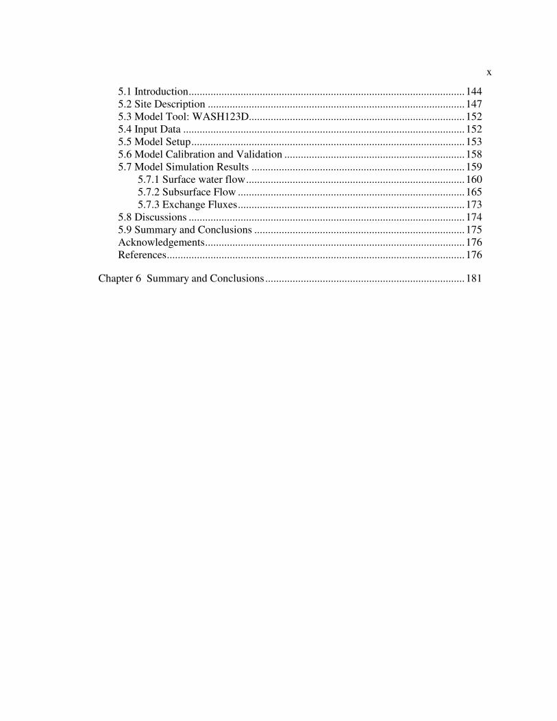
5.1 Introduction.....................................................................................................144
5.2 Site Description ..............................................................................................147
5.3 Model Tool: WASH123D...............................................................................152
5.4 Input Data .......................................................................................................152
5.5 Model Setup....................................................................................................153
5.6 Model Calibration and Validation ..................................................................158
5.7 Model Simulation Results ..............................................................................159
5.7.1 Surface water flow................................................................................160
5.7.2 Subsurface Flow ...................................................................................165
5.7.3 Exchange Fluxes...................................................................................173
5.8 Discussions .....................................................................................................174
5.9 Summary and Conclusions .............................................................................175
Acknowledgements...............................................................................................176
References.............................................................................................................176
Chapter 6 Summary and Conclusions.........................................................................181
xi
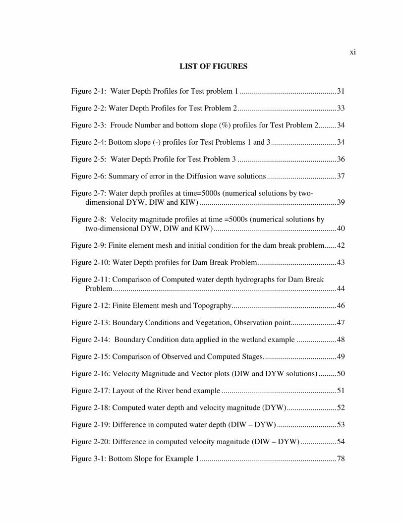
LIST OF FIGURES
Figure 2-1: Water Depth Profiles for Test problem 1.................................................31
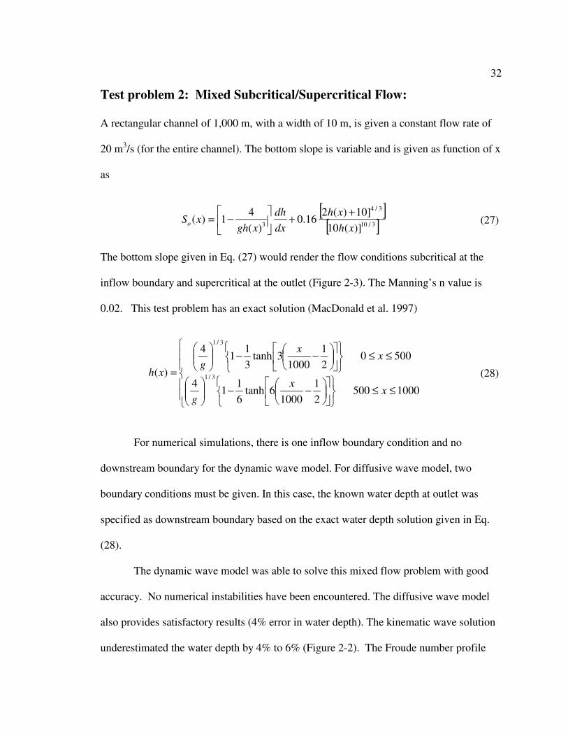
Figure 2-2: Water Depth Profiles for Test Problem 2..................................................33
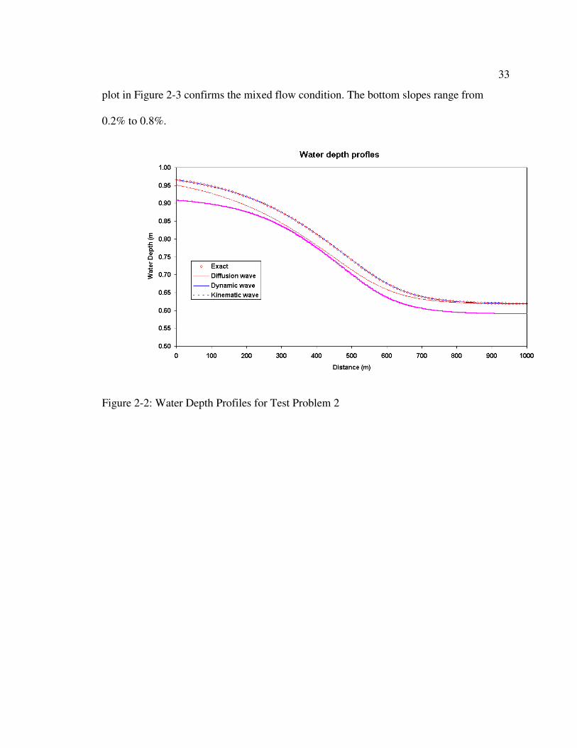
Figure 2-3: Froude Number and bottom slope (%) profiles for Test Problem 2.........34
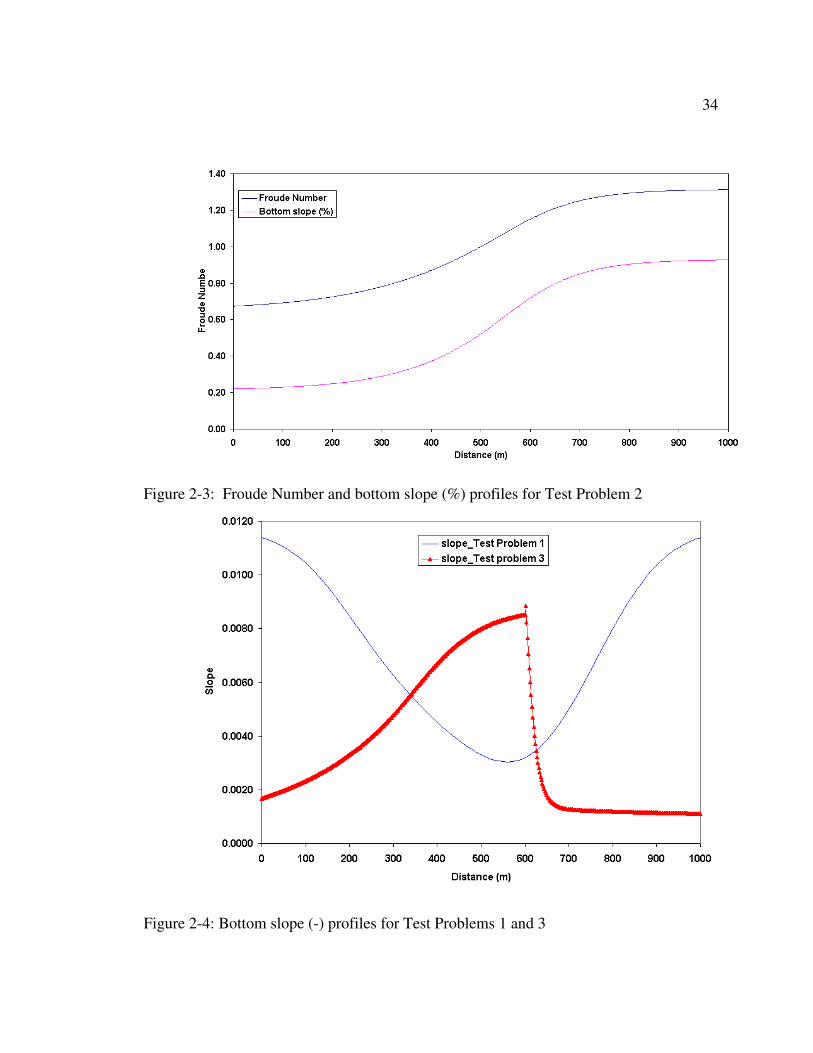
Figure 2-4: Bottom slope (-) profiles for Test Problems 1 and 3.................................34
Figure 2-5: Water Depth Profile for Test Problem 3 ..................................................36
Figure 2-6: Summary of error in the Diffusion wave solutions ...................................37
Figure 2-7: Water depth profiles at time=5000s (numerical solutions by two-
dimensional DYW, DIW and KIW) .....................................................................39
Figure 2-8: Velocity magnitude profiles at time =5000s (numerical solutions by
two-dimensional DYW, DIW and KIW)..............................................................40
Figure 2-9: Finite element mesh and initial condition for the dam break problem......42
Figure 2-10: Water Depth profiles for Dam Break Problem........................................43
Figure 2-11: Comparison of Computed water depth hydrographs for Dam Break
Problem.................................................................................................................44
Figure 2-12: Finite Element mesh and Topography.....................................................46
Figure 2-13: Boundary Conditions and Vegetation, Observation point.......................47
Figure 2-14: Boundary Condition data applied in the wetland example ....................48
Figure 2-15: Comparison of Observed and Computed Stages.....................................49
Figure 2-16: Velocity Magnitude and Vector plots (DIW and DYW solutions) .........50
Figure 2-17: Layout of the River bend example ..........................................................51
Figure 2-18: Computed water depth and velocity magnitude (DYW).........................52
Figure 2-19: Difference in computed water depth (DIW – DYW)..............................53
Figure 2-20: Difference in computed velocity magnitude (DIW – DYW) ..................54
Figure 3-1: Bottom Slope for Example 1.....................................................................78
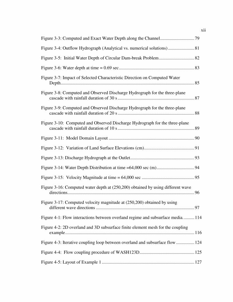
xii
Figure 3-3: Computed and Exact Water Depth along the Channel..............................79
Figure 3-4: Outflow Hydrograph (Analytical vs. numerical solutions) .......................81
Figure 3-5: Initial Water Depth of Circular Dam-break Problem...............................82
Figure 3-6: Water depth at time = 0.69 sec..................................................................83
Figure 3-7: Impact of Selected Characteristic Direction on Computed Water
Depth.....................................................................................................................85
Figure 3-8: Computed and Observed Discharge Hydrograph for the three-plane
cascade with rainfall duration of 30 s ...................................................................87
Figure 3-9: Computed and Observed Discharge Hydrograph for the three-plane
cascade with rainfall duration of 20 s ...................................................................88
Figure 3-10: Computed and Observed Discharge Hydrograph for the three-plane
cascade with rainfall duration of 10 s ...................................................................89
Figure 3-11: Model Domain Layout ...........................................................................90
Figure 3-12: Variation of Land Surface Elevations (cm)............................................91
Figure 3-13: Discharge Hydrograph at the Outlet........................................................93
Figure 3-14: Water Depth Distribution at time =64,000 sec (m).................................94
Figure 3-15: Velocity Magnitude at time = 64,000 sec ..............................................95
Figure 3-16: Computed water depth at (250,200) obtained by using different wave
directions...............................................................................................................96
Figure 3-17: Computed velocity magnitude at (250,200) obtained by using
different wave directions ......................................................................................97
Figure 4-1: Flow interactions between overland regime and subsurface media. .........114
Figure 4-2: 2D overland and 3D subsurface finite element mesh for the coupling
example.................................................................................................................116
Figure 4-3: Iterative coupling loop between overland and subsurface flow ................124
Figure 4-4: Flow coupling procedure of WASH123D................................................125
Figure 4-5: Layout of Example 1 .................................................................................127

xiii
Figure 4-6: Comparison of Outflow Hydrographs.......................................................128
Figure 4-7: Comparison of Total Exchange Fluxes .....................................................129
Figure 4-8: Schematic layout of the wetland example.................................................131
Figure 4-9: Comparison of computed water levels. .....................................................132
Figure 4-10: Three-dimensional finite element mesh ..................................................135
Figure 4-11: Pressure head distribution at x=500 m (time=14200 seconds) ..............136
Figure 4-12: Pressure head distribution at y=430 m (time=14200 seconds) ...............137
Figure 4-13: Computed Discharge hydrographs (coupled flow with different
approaches) ...........................................................................................................138
Figure 5-1: Location Map of ENR (SFWMD, 2000)...................................................149
Figure 5-2 Schematic Map of ENR (Modified after SFWMD, 2000) .........................150
Figure 5-3: Vegetation types as simulated in the model ..............................................155
Figure 5-4: Finite Element Meshes for ENR Basin with Soil Types..........................158
Figure 5-5: Simulated and Observed Surface Water Levels at ENR101 .....................162
Figure 5-6: Simulated and Observed Surface Water Levels at ENR301 .....................163
Figure 5-7: Simulated and Observed Surface Water Levels at ENR203 .....................164
Figure 5-8: Simulated and Observed Surface Water Levels at ENR401 ....................165
Figure 5-9: Simulated and Observed Groundwater Levels at ENR102GW ................167
Figure 5-10: Simulated and Observed Groundwater Levels at ENR303GW ..............168
Figure 5-11: Simulated and Observed Groundwater Levels at ENR203GW ..............169
Figure 5-12: Simulated and Observed Groundwater Levels at ENR401GW ..............170
Figure 5-13: Simulated Total Head Distribution (ft NGVD) on 2/4/1998. ................171
Figure 5-14: Location of Transects and Lithology of ENR (after Harvey et al.,
2002) .....................................................................................................................172

xiv
Figure 5-15: Total Head Distribution (2/4/1998) for two transects of ENR (ft
NGVD). ................................................................................................................173
Figure 5-16: Distribution of Computed Vertical Flux (cm/day) (7/10/1998) ..............174
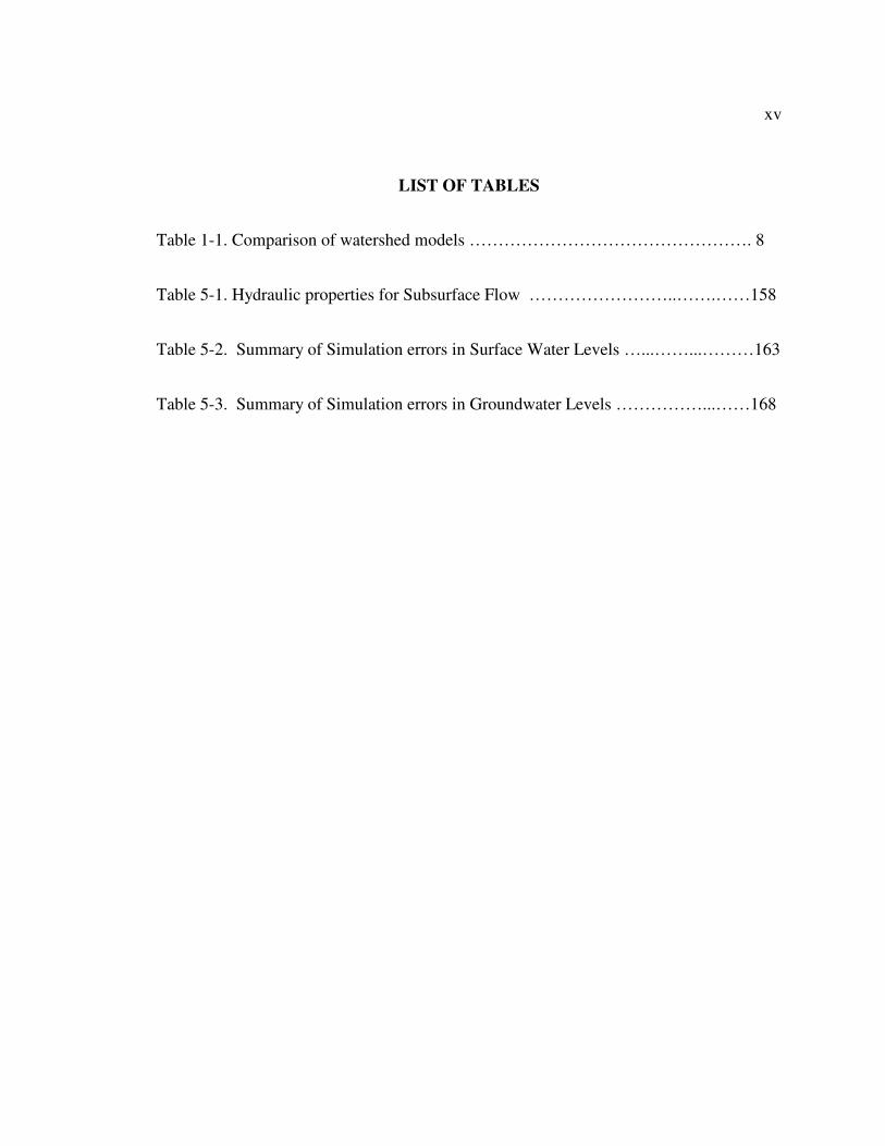
xv
LIST OF TABLES
Table 1-1. Comparison of watershed models …………………………………………. 8
Table 5-1. Hydraulic properties for Subsurface Flow ……………………..…….……158
Table 5-2. Summary of Simulation errors in Surface Water Levels …...……...………163
Table 5-3. Summary of Simulation errors in Groundwater Levels ……………...……168
xvi
ACKNOWLEDGEMENTS
I am very grateful for the support and encouragement of Dr. Gour-Tsyh Yeh
throughout my graduate study.
I would also like to thank my other committee members, Dr. Arthur Miller, Dr.
Christopher Duffy and Dr. Derek Elsworth for their time and effort on this thesis.
I am indebted to my family for their support and patience that have enabled me to
successfully complete this work.
Last but not least, University of Central Florida (UCF) provided resources and
facilities that were needed for my research in 2000 through 2002 when I conducted my
research off the Penn State University (PSU) campus with my thesis Advisor, Dr. Gour-
Tsyh Yeh who moved from Penn State to UCF in August 2000.
1
Chapter 1
Introduction
1.1 Overview of the Mathematical Modeling of Watersheds
A watershed model is an integrated representation of nearly any hydrological
process of the hydrologic cycle; major processes within a watershed include precipitation,
interception, evapotransiration, infiltration, overland flow, channel/stream flow, and
subsurface flow.
Watershed models are essential tools used to address various water resources and
environmental protection problems (Singh and Frevert, 2006). The mathematical
modeling of watersheds has been extensive since the creation of modern digital
computers in the 1950s (Singh and Woolhiser, 2002). There is a plethora of all kinds of
watershed models, ranging from purely empirical, black box type models to physics
based, integrated models.
Many lumped or semi-distributed watershed models are similar in model structure
and principle. The well-known conceptual Stanford watershed model (Crawford and
Linsley, 1966) and its successor, HSPF (Donigian and Imhoff, 2006), are representative
2
of these watershed model types. The model structure is based on water balance in
predefined conceptual storage zones, and model parameters are often without clear
physical meaning. The limitation of lumped watershed models is well known - model
parameters must be calibrated with historic data; estimated parameters are not
transferable and distributed information on flow velocity and water depth cannot be
provided for water quality modeling.
The development of watershed models is often guided by an intentional application and
modeling objective. When information on the total quantity and timing of surface runoff
at the watershed outlet (such as in flood control) is enough for the modeling objective, the
traditional lumped watershed models can be used if historic data is available, in order to
calibrate the model. But in other cases, such as non-point source pollution, soil erosion,
land use effect, climate change, etc., users need information about the flow field (water
velocity and depth distribution) or the timing of any extensive alterations to the
watershed system from land use or deforestation; from here, a physics based, distributed
hydrologic model is necessary. There are also great needs in real-world water
management for such integrated models. For example, the importance of surface water
and groundwater interaction has led to integrated models developed by local government
agencies in South Florida (Lal et al., 2005) and California (LaBolle et al., 2003).
Since Freeze and Harlan published their blueprint for a three-dimensional model
of watersheds (Freeze and Harlan, 1969) more than three decades ago, there has been
much progress in this field. The SHE and its derivatives MIKE SHE are very popular in
3
Europe (Abbott et al., 1986). In the United States, the CASC2D and its newest version
GSSHA (Downer, 2004) is a finite difference code that can do integrated modeling in a
less rigorous approach. There are some model codes developed around the popular
MODFLOW groundwater model [for example, MODBRANCH (Swain and Wexler
(1996), MOD-HMS (Panday and Huyakorn (2004)].
There has been much debate and controversy on physics based, distributed
watershed models (e.g., Grayson et al., 1992; Woolhiser, 1996; Beven, 2002 and Loague
and VanderKwaak, 2004). Beven (2002) concluded that a radical change in paradigm is
needed for watershed models. The Freeze and Harlan (1969) blueprint is however,
flawed, and will eventually be abandoned. For instance, a major flaw is related to both
scale (the point-scale mechanistic partial differential equations may not be valid at model
grid scale) and equifinality (model over-parameterization).
Reggiani et al. (1998, 1999, 2000 and 2005) offer an alternative watershed model
structure based on the discretization of a watershed into spatial units, termed
‘representative elementary watersheds’ (REWs). The point-scale conservation equations
for mass, momentum, and energy is integrated over a sub-watershed. This flux-based
formulation approach can be traced back to earlier research by Duffy (1996). The
difficulties in determining hydrological fluxes are a major problem and, if the size of
REWs is very small, it will run into the same scale problem as the point-scale, physics
based models. On the other hand, if the size of REWs is large, the physical meaning of
4
state variables, such as flow velocity, pressure head, and water depth, are only nominal at
best.
Young (2003) offers another alternative, termed the ‘data based mechanistic
approach’; its use is intended for hydrologic models. It is said to be a stochastic model
with a top-down approach that can incorporate physical reasoning into the statistical
model. This approach is better suited for practical application (e.g., real-time flood
forecasting) and not for what-if type explanation-oriented modeling.
In the proceeding chapters, the Freeze and Harlan (1969) blueprint of a physics
based, three-dimensional watershed model (as a viable modeling approach for integrated
watershed models) will be explored. The increasing availability of spatially distributed
hydrological data through remote sensing, radar rainfall, GIS, and new measurement
techniques also support such physics-based distributed models.
1.2 Physics-based, integrated watershed models
The mechanistic, process-oriented modeling of fluid flow in watersheds can be
conveniently divided into flow component models and coupling mechanism. There have
been extensive studies on component models (for example, overland flow models,
channel network flow models, and subsurface flow models) and among them; the flow
component coupling is another important issue.
5
Water flow components in a watershed are essentially comprised of surface water
and subsurface flow, where ‘surface water flows’ include overland and channel flow.
There are at least three distinct runoff generation mechanisms. The first one is the
Hortonian overland flow mechanism’, usually called ‘infiltration excess mechanism’.
This has been the dominant concept in the current generation of surface hydrologic
models. Under this paradigm, overland flow was extensively modeled, but the
infiltration and subsurface flow components are treated empirically, as a water sink/loss.
Field observation and further research have demonstrated that Hortonian overland flow is
rare and of little impact in humid, forested regions, while the subsurface storm flow
mechanism is the major contribution to runoff. In this case, most rainfall is to be
absorbed by the soil, and subsurface flow becomes an important contribution to stream
flow. Another runoff generation mechanism is called saturated excess, which represents
the runoff process in place such as wetlands where the soil is saturated most of the time.
Only a physics-based, integrated watershed models can simulate all these runoff
generation mechanisms in a single model.
1.3 Motivation and Objectives
The watershed modeling in the past 30 years has been focused on individual flow
components, e.g., overland flow, channel flow, groundwater flow, etc. Most overland
flow modeling studies did not couple with subsurface flow and, in subsurface hydrology,
the surface water processes were often only considered as a simple source/sink. When
6
coupling is considered, weak coupling or artificially created linkage terms are often used
for flux-exchange calculations.
Freeze and Harlan (1969) were the first to develop a blueprint of the physically
based watershed model. Smith and Woolhiser (1972) were one of the first to apply the
one-dimensional Richards' equation for unsaturated flow in their overland model with a
1-D kinematic wave equation. Akan and Yen (1981) coupled a two-dimensional
subsurface flow component with overland flow. One of the first attempts to build a
comprehensive numerical model of a watershed based on the Freeze and Harlan blueprint
is the SHE model in Europe (Abbott et al., 1986). In the SHE watershed model, the
unsaturated zone is represented with one-dimensional Richards' equation. In USA, the
focus has been toward a practical engineering application, so most of the watershed
models are lumped. Among the few physically based models developed are CASC2D by
Julien et al. (1995) and KINEROS by Woolhiser et al. (1990). CASC2D included the
diffusion wave approximation of overland flow and channel flow; infiltration is based on
the Green and Ampt model and the explicit finite difference method is used. KINEROS is
based on the kinematic wave model for overland flow routing with empirical infiltration
equations.
This thesis research concerns with the physics based, integrated mathematical
modeling of watershed hydrology and hydraulics. The computational aspect of physics-
based, integrated watershed models is investigated in term of proper selection of
governing equations, coupling approaches, and numerical methods, etc. The hydrology
7
and hydraulics modules of the watershed model are particularly designed as the basis for
modeling transport of sediments and pollutant at watershed scales.
Some recently developed physics-based, integrated watershed models are briefly
compared in Table 1-1. All of these models apply Richards’ equation for subsurface flow;
however, the governing equations for surface flow, numerical methods and coupling
approach are quite different. Therefore, several critical issues are still in need of further
study, even though the Freeze and Harlan (1969) blueprint was proposed more than three
decades ago.
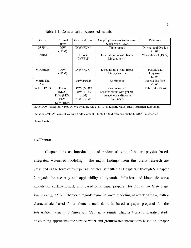
8
Table 1-1: Comparison of watershed models
Code Channel
flow
Overland flow Coupling between Surface and
Subsurface Flows
Reference
GSSHA
DIW
(FDM)
DIW (FDM) Time-lagged Downer and Orgden
(2004)
INHM
DIW (
CVFEM)
Discontinuous with linear
Linkage-terms
VanderKwaak(1999)
MODHMS DIW
(FDM)
DIW (FDM)
Discontinuous with linear
Linkage-terms
Panday and
Huyakorn
(2004)
Morita and
Yen
DIW(FDM) Continuous Morita and Yen
(2002)
WASH123D DYW
(MOC)
DIW (FEM,
ELM)
KIW (ELM)
DYW (MOC)
DIW (FEM,
ELM)
KIW (ELM)
Continuous or
Discontinuous with general
linkage terms (linear or
nonlinear)
Yeh et al. (2006)
Note: DIW: diffusion wave; DYW: dynamic wave; KIW: kinematic wave; ELM: Eulerian-Lagragian
method; CVFEM: control volume finite element; FDM: finite difference method; MOC: method of
characteristics.
1.4 Format
Chapter 1 is an introduction and review of state-of-the art physics based,
integrated watershed modeling. The major findings from this thesis research are
presented in the form of four journal articles, self titled as Chapters 2 through 5. Chapter
2 regards the accuracy and applicability of dynamic, diffusion, and kinematic wave
models for surface runoff; it is based on a paper prepared for Journal of Hydrologic
Engineering, ASCE. Chapter 3 regards dynamic wave modeling of overland flow, with a
characteristics-based finite element method; it is based a paper prepared for the
International Journal of Numerical Methods in Fluids. Chapter 4 is a comparative study
of coupling approaches for surface water and groundwater interactions based on a paper
9
intended for submission to the Journal of Hydrology. Chapter 5 is an application on
surface water and groundwater interactions in a constructed wetland, based on a paper
prepared for possible publication on Journal of Hydrologic Engineering, ASCE. The last
chapter, Chapter 6, is summary of work presented and a presentation of suggested
research and future applications.
References
Abbot M.B., Bathurst J.C., Cunge J.A., O’Connell P.E., Rasmussen J. (1986), “An
introduction to the European Hydrologic System-Systeme Hydrologique Europeen,
SHE, 2: Structure of a physically-based, distributed modeling system.’’ Journal of
Hydrology 87: 61–77.
Akan AO, Yen BC. (1981), Mathematical model of shallow water flow over porous
media. Journal of Hydraulics Division, American Society of Civil Engineers 107:
479–494.
Beven K., (2002), Towards an alternative blueprint for a physically based digitally
simulated hydrologic response modeling system, Hydrological Processes, 16, 189-
202.
10
Crawford NH, Linsley RS., (1966), Digital Simulation in Hydrology: The Stanford
Watershed Model IV. Technical Report no. 39, Department of Civil Engineering,
Stanford University, Palo Alto, CA.
Donigian, A.S. and J. Imhoff. (2006), Chapter 2: History and evolution of watershed
modeling derived from the Stanford Watershed model, in Watershed Models. Eds. By
Singh VP and Frevert, CRC Press, Boca Raton, FL.
Downer, C.W. and Ogden, F.L., (2004), GSSHA: Model to simulate diverse stream flow
producing processes. Journal of Hydrological Engineering, 9 (3): 161-174.
Duffy C.J. (1996), “A two-state integral-balance model for soil moisture and groundwater
dynamics in complex terrain.” Water Resources Research 32: 2421–2434.
Freeze R.A. and Harlan R.L., (1969) “Blueprint for a physically-based digitally-
simulated hydrologic response model.” Journal of Hydrology, 9, pp. 237–258.
Grayson RB, Moore ID, McMahon TA. (1992), Physically-based hydrologic modelling.
2. Is the concept realistic? Water Resources Research 28: 2659.
Julien, P. Y., Saghafian, B., and Ogden, F. L. (1995), ‘‘Raster-based hydrologic modeling
of spatially varied surface runoff.’’ Water Resour. Bull., 31(3), 523–536.
11
LaBolle EM, Ahmed AA, Fogg GE. (2003), Review of the Integrated Groundwater and
Surface-Water Model (IGSM), Ground Water. 2003 Mar-Apr;41(2):238-46.
Lal W., Van Zee R. and Belnap M. (2005), Case Study: Model to Simulate Regional
Flow in South Florida. J. Hydr. Engrg., Volume 131, Issue 4, pp. 247-258 (April
2005).
Loague K, VanderKwaak JE. (2004), Physics-based hydrologic response simulation:
platinum bridge, 1958 Edsel or useful tool. Hydrological Processes 18: 2949–2956.
Loague K, VanderKwaak JE.(2002), Simulating hydrologic response for the R-5
catchment: comparison of two models and the impact of the roads. Hydrological
Processes 16: 1015–1032.
Panday S. and Huyakorn P.S. (2004), A fully coupled physically-based spatially-
distributed model for evaluating surface/subsurface flow. Advances in Water
Resources, 27 (2004) 361–382
Reggiani P., Sivapalan M., Hassanizadeh S.M. (1998), A unifying framework for
watershed thermodynamics: balance equations for mass, momentum, energy and
entropy and the second law of thermodynamics. Advances in Water Resources 23(1):
15–40.
12
Reggiani P, Hassanizadeh SM, Sivapalan M, Gray WG. (1999), A unifying framework
for watershed thermodynamics: constitutive relationships. Advances in Water
Resources 23(1): 15–40.
Reggiani, P., M. Sivapalan, and S. M. Hassanizadeh (2000), Conservation equations
governing hillslope responses, Water Resour. Res., 38(7), 1845– 1863.
Reggiani, P., and T. H. M. Rientjes (2005), Flux parameterization in the representative
elementary watershed approach: Application to a natural basin, Water Resour. Res.,
41, W04013, doi:10.1029/2004WR003693.
Singh V.P. and Frevert D. K., editors. (2006), Watershed Models. CRC Press, Boca
Raton, FL USA.
Singh V. P. and Woolhiser D.A., (2002), Mathematical modeling of watershed
hydrology, Journal of Hydrologic Engineering, Vol. 7, No.4, July 1, 2002.
Swain ED, Wexler EJ, (1996), A coupled surface-water and groundwater flow model for
simulation of stream–aquifer interaction. US Geological Survey Techniques of water-
resources investigations, Book 6; 1996. 125 p [chapter A6].
13
VanderKwaak, J. (1999), “Numerical simulation of flow and chemical transport in
integrated surface-subsurface hydrologic systems.” Ph.D. Thesis, University of
Waterloo, Waterloo, Canada. 217 pp.
Woolhiser, D. A., Smith, R. E., and Goodrich, D. C. (1990), ‘‘KINEROS—A kinematic
runoff and erosion model: Documentation and user manual.’’ Rep. No. ARS-77,
USDA, Washington, D.C.
Woolhiser, D.A. (1996), Search for physically based runoff model – a hydrologic El
Dorado? Journal of Hydrologic Engineering, Vol. 122, 122-129.
Yeh, G.T., G. B. Huang, H. P. Cheng, F. Zhang, H. C. Lin, E. Edris, and D. Richards.
(2006), Chapter 9: A first principle, physics-based watershed model: WASH123D, in
Watershed Models. Eds. By Singh VP and Frevert, CRC Press, Boca Raton, FL.
Young, P. C. (2003), Top-down and data-based mechanistic modelling of rainfall-flow
dynamics at the catchment scale, Hydrol. Processes, 17, 2195-2217.
14
Chapter 2
On simulating surface water flows with dynamic, diffusion and kinematic waves
Abstract
The complete Saint Venant equations/two-dimensional shallow water equations
(dynamic wave equations) and the kinematic wave or diffusion wave approximations
were implemented for one-dimensional channel network flow and two-dimensional
overland flow in a watershed model, WASH123D. Careful choice of numerical methods
is needed even for the simple kinematic wave model. Since the kinematic wave equation
is of pure advection, the backward method of characteristics is used for the kinematic
wave model. A characteristics based finite element method is chosen for the hyperbolic-
type dynamic wave model. The Galerkin finite element method is used to solve the
diffusion wave model. Diffusion wave and kinematic wave approximations are found in
many surface runoff routing models. The error in these models has been characterized as
overland/channel flow over simple geometry in some cases. However, the nature and
propagation of these approximation errors under complex two-dimensional flow
conditions are not well known. These issues are evaluated within WASH123D by
comparison of simulation results for several example problems. The accuracy of the three
wave models for one-dimensional channel flow was evaluated with several non-trivial
(trans-critical flow; varied bottom slopes with frictions and non-prismatic cross-section)
15
benchmark problems, and for two-dimensional overland flow with dam-break problems
and a wetland example. The applicability of dynamic-wave, diffusion-wave and
kinematic-wave models to real watershed modeling is discussed with simulation results
from these numerical experiments. It was concluded that kinematic wave model could
lead to significant errors in most applications. On the other hand, the diffusion wave
model is adequate for modeling overland flow in most natural watersheds. The complete
dynamic wave equations are more accurate in low-terrain areas, such as flood plains, are
more suitable for river flow at river bends and transient fast flow situations.
2.1 Introduction
Diffusion wave and kinematic wave approximations are found in many surface runoff
flow routing models. The error in these models has been characterized for some cases of
overland flow over simple, often one-dimensional geometry. Ponce et al. (1978)
presented a criterion for the applicability of kinematic and diffusion waves models in
surface flow derived from theoretical analysis on the linearized Saint Venant equations.
Govindaraju et al. (1988, 1990) studied diffusion wave models for steady overland flow
and approximate analytical solutions. Parlange et al. (1990) derived and estimated errors
in kinematic and diffusion wave models for steady state overland flow on a single plane
by comparing numerical simulations with numerical solutions of the full Saint Venant
equations; they demonstrated that, in case where a kinematic wave is not accurate, use of
a diffusion wave would not produce a noticeable difference. Through the analysis of
relative magnitude of the acceleration terms in the governing equations, Richardson and
16
Julien (1994) concluded that diffusion wave approximation of overland flow is not
suitable for supercritical flow condition. Singh and coworkers (e.g., Singh et al., 2005
Moramarco and Singh; 2002 and Singh and Aravamuthan, 1995) published a series of
papers on the accuracy and error estimation of diffusion and kinematic waves overland
flow on a plane by numerical experiments and concluded that diffusion wave
approximation is fairly accurate for most overland flow conditions. Tayfur et al. (1993)
compared numerical solutions of dynamic, diffusive and kinematic wave models for two-
dimensional overland flow on rough surfaces with an average steep slope of 0.086; the
results are essentially the same due to the steep slope. However, the nature and
propagation of these approximation errors under more complex two-dimensional surface
water flow conditions are not well known.
While diffusion wave approximation is a widely applied model in many current
watershed models, kinematic wave approximation is prevailing in many current
watershed models in research and practice (for example, HEC-HMS [Hydrologic
Engineering Center(HEC), 2000], HSPF[Donigian and Imhoff, 2006], SWMM[Metcalf
and Eddy et al. 1971] and some new GIS-based watershed models [e.g., Fortin and
Turcotte et al., 2001; Olivera and Maidment, 1999]). This is attributed to its simplicity
and ease of numerical solutions for kinematic wave models. However, significant error
could be possible for kinematic wave models.
For one-dimensional channel flow, the fully dynamic wave approach has been
implemented in many well-established stand-alone stream network flow models. These
17
dynamic wave channel network flow models are usually externally linked to traditional
lumped watershed models for practical application of flow routing. Again, diffusion
wave and kinematic wave approximations are popular in channel network flow module of
most integrated watershed models.
The complete Saint Venant equations/two-dimensional shallow water equations
(dynamic wave equations) and the kinematic wave or diffusion wave approximations
were all implemented for one-dimensional channel network flow and two-dimensional
overland flow in a watershed model, WASH123D. We will present some numerical
experiments on these three options for overland flow and channel flow and demonstrate
the potential errors in using one single wave model for all flow situations.
The research objectives include:
1. Apply accurate and stable numerical solutions of dynamic, kinematic and
diffusion wave models;
2. Demonstrate applicability and limitations of kinematic and diffusion wave
models by comparison with fully dynamic wave model through numerical
experiments.
2.2 Governing Equations
The governing equations for surface water flows in a watershed can be derived
from the conservation of water mass and momentum. The depth-averaged two-
18
dimensional shallow water equations and the cross-section-averaged one-dimensional
Saint Venant equations are considered accurate representations of two-dimensional
overland flow and one-dimensional channel network flow, respectively. Only equations
for two-dimensional overland flow are described in detail, as follows.
2.2.1 Dynamic wave equations
The depth-averaged 2D shallow water equations for overland flow in matrix form
are:
Gy
F
x
F
t
U yx =∂
∂+
∂
∂+
∂
∂ (1)
The conservative variables are U=(h, uh, vh); h is water depth; u is the velocity
component in the x-direction; v is the velocity component in the y-direction, respectively.
The flux vector F has two components Fx and Fy:
22
0
202
, , ( )2
( )
2
x y x fx
y fy
uhvh S
ghF u h F uvh G gh S S
gh S Sghuvh v h
= + = = − − +
(2)
where SSIERS +−−= , is the source/Sink term as a result of rainfall (R),
evapotranspiration (E) and infiltration (I), and human-induced source/sink (SS), etc. The
eddy turbulent term, momentum exchange flux, surface shear stress (wind effect), etc.
have been omitted from the momentum equations for the sake of simplicity of
presentation.
19
The bed slopes are defined as:
y
ZS
x
ZS yx
∂
∂−=
∂
∂−= 0
00
0 , (3)
where g is gravitational acceleration and Z0 is the bed elevation above a datum.
The friction slopes can be approximated by the Manning’s equation as:
3/4
222
3/4
222
,h
vuvnS
h
vuunS fyfx
+=
+= (4)
where n is the Manning’s roughness coefficient.
Boundary conditions for two-dimensional dynamic wave models (DYW) of
overland flow are based on physical flow conditions at the boundary; there can be zero,
one or two boundary conditions at the inflow and outflow boundaries based on
supercritical, subcritical flow or critical flow conditions.
For one-dimensional channel network flow, Equations (1) through (4) can be
applied with all variables in the y-direction being null for prismatic, rectangular cross-
section channels. For channels with arbitrary shape cross-sections, the water depth (h) is
replaced with the cross-sectional area (A) and some terms need to be adjusted.
20
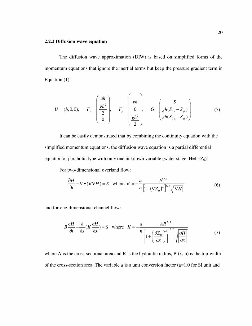
2.2.2 Diffusion wave equation
The diffusion wave approximation (DIW) is based on simplified forms of the
momentum equations that ignore the inertial terms but keep the pressure gradient term in
Equation (1):
2
0
20
( ,0,0), , 0 , ( )2
( )0
2
x y x fx
y fy
uhvh S
ghU h F F G gh S S
gh S Sgh
= = = = − −
(5)
It can be easily demonstrated that by combining the continuity equation with the
simplified momentum equations, the diffusion wave equation is a partial differential
equation of parabolic type with only one unknown variable (water stage, H=h+Z0):
For two-dimensional overland flow:
SHKt
H=∇•∇−
∂
∂)( where
( )[ ] HZ
h
n
aK
∇∇+−=
3/22
0
3/5
1 (6)
and for one-dimensional channel flow:
Sx
HK
xt
HB =
∂
∂
∂
∂−
∂
∂)( where
x
H
x
Z
AR
n
aK
∂
∂
∂
∂+
−=3/2
2
0
3/2
1
(7)
where A is the cross-sectional area and R is the hydraulic radius, B (x, h) is the top-width
of the cross-section area. The variable a is a unit conversion factor (a=1.0 for SI unit and
21
a=1.486 for US Customary units). The term:
2
01
∂
∂+
x
Zcan be considered as a factor that
accounts for increased shear stress caused by a sloping land surface.
Both upstream (inflow) and downstream (outflow) boundary conditions are
needed for the diffusion wave model. For two-dimensional overland flow, usually, no-
flow condition is applied at the upstream watershed boundary and at the watershed outlet,
a specified water stage or a stage-discharge rating curve (e.g., critical flow or zero-depth
gradient condition) are imposed.
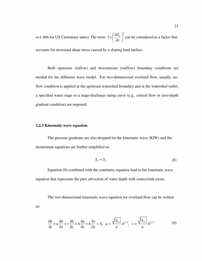
2.2.3 Kinematic wave equation
The pressure gradients are also dropped for the kinematic wave (KIW) and the
momentum equations are further simplified as:
fSS =0 (8)
Equation (8) combined with the continuity equation lead to the kinematic wave
equation that represents the pure advection of water depth with source/sink terms.
The two-dimensional kinematic wave equation for overland flow can be written
as:
00 2 / 3 2 / 3, , yx
SSh h h u vu v h h S u h v h
t x y x y n n
∂ ∂ ∂ ∂ ∂+ + + + = = =
∂ ∂ ∂ ∂ ∂ (9)
22
By replacing the velocity (u,v) with the velocity formula, the kinematic wave
equation is in a form of pure advection of water depth (h) with source term. Since
kinematic wave contain only one characteristic in the downstream direction, no
downstream boundary is needed. Therefore, backwater effect cannot be considered.
2.3 Numerical Methods
2.3.1 Dynamic wave model
The widespread application of diffusion and kinematic wave approximation of
surface water flow routing in physics-based watershed models can be attributed to the
fact that, numerical solutions of the full shallow water equations, under complex
topography and transient, distributed forcing (e.g., rainfall and infiltration), are
computationally intensive; furthermore, it suffers from numerical stability and
convergence problems. Indeed, in rainfall-runoff/overland flow simulations, the full
dynamic wave equations are rarely applied and, when applied, they are limited to small-
scale geometry (experiment plots or single hillslopes) (for an example, see Chow and
Ben-Zvi, 1973; Zhang and Cundy, 1989; Fielder and Ramirez, 2000). Therefore, making
a careful and judicious choice regarding the numerical method for a dynamic wave model
is critical. We consider the characteristics-based finite element method to be a natural
choice based on flow physics of the full shallow water equations.
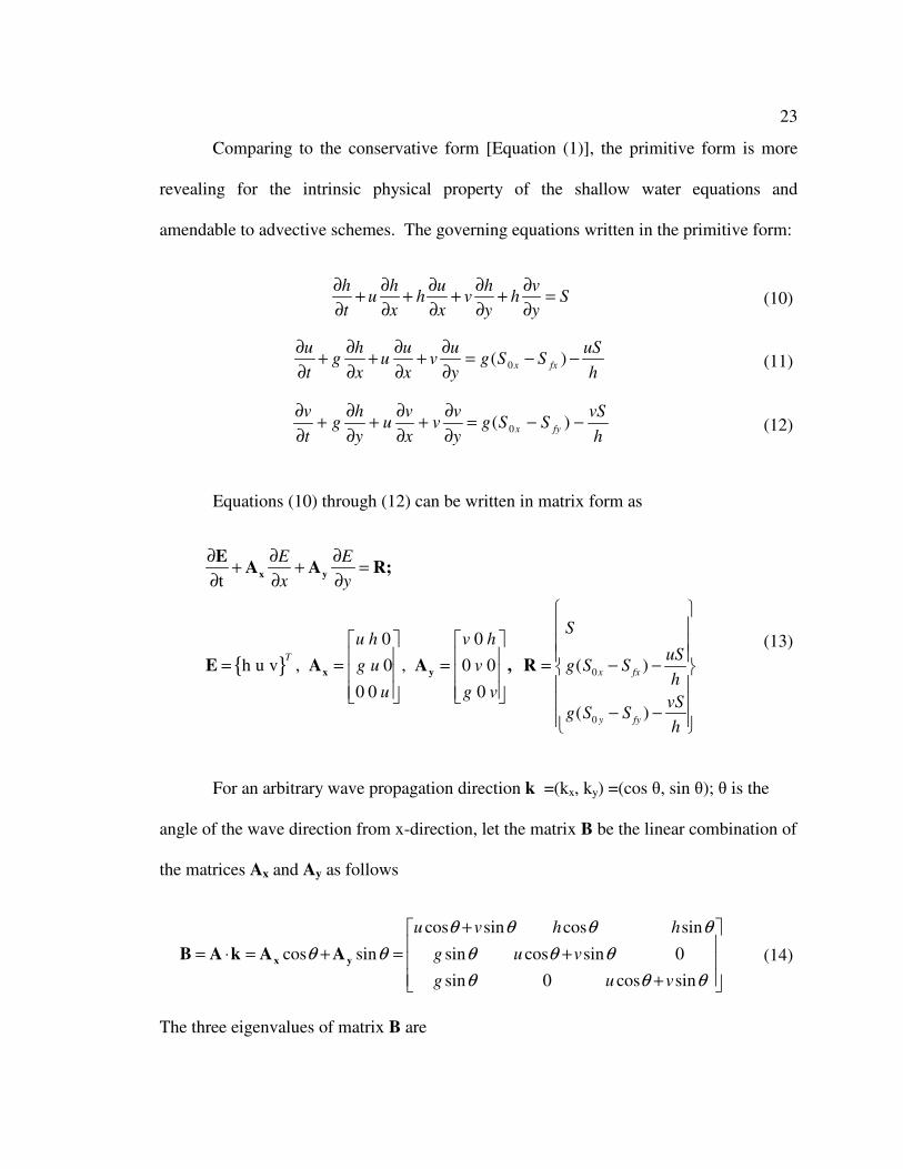
23
Comparing to the conservative form [Equation (1)], the primitive form is more
revealing for the intrinsic physical property of the shallow water equations and
amendable to advective schemes. The governing equations written in the primitive form:
Sy
vh
y
hv
x
uh
x
hu
t
h=
∂
∂+
∂
∂+
∂
∂+
∂
∂+
∂
∂ (10)
h
uSSSg
y
uv
x
uu
x
hg
t
ufxx −−=
∂
∂+
∂
∂+
∂
∂+
∂
∂)( 0 (11)
h
vSSSg
y
vv
x
vu
y
hg
t
vfyx −−=
∂
∂+
∂
∂+
∂
∂+
∂
∂)( 0 (12)
Equations (10) through (12) can be written in matrix form as
{ } 0
0
t
0 0
h u v , 0 , 0 0 ( )
0 0 0
( )
T
x fx
y fy
E E
x y
Su h v h
uSg u v g S S
hu g v
vSg S S
h
∂ ∂ ∂+ + =
∂ ∂ ∂
= = = = − −
− −
x y
x y
EA A R;
E A A , R
(13)
For an arbitrary wave propagation direction k =(kx, ky) =(cos θ, sin θ); θ is the
angle of the wave direction from x-direction, let the matrix B be the linear combination of
the matrices Ax and Ay as follows
+
+
+
=+=⋅=
θθθ
θθθ
θθθθ
θθ
sincos0sin
0sincossin
sincossincos
sincos
vug
vug
hhvu
yx AAkAB (14)
The three eigenvalues of matrix B are
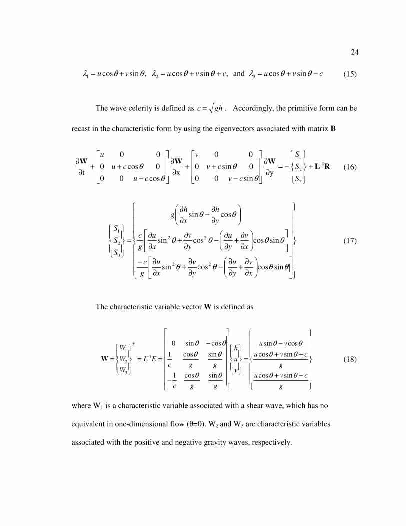
24
1 2 3cos sin , cos sin , and cos sinu v u v c u v cλ θ θ λ θ θ λ θ θ= + = + + = + − (15)
The wave celerity is defined as ghc = . Accordingly, the primitive form can be
recast in the characteristic form by using the eigenvectors associated with matrix B
1
2
3
0 0 0 0
0 cos 0 0 sin 0t x y
0 0 cos 0 0 sin
Su v
u c v c S
u c v c S
θ θ
θ θ
−
∂ ∂ ∂ + + + + = − + ∂ ∂ ∂ − −
1W W WL R (16)
∂
∂+
∂
∂−
∂
∂+
∂
∂−
∂
∂+
∂
∂−
∂
∂+
∂
∂
∂
∂−
∂
∂
=
θθθθ
θθθθ
θθ
sincoscossin
sincoscossin
cossin
22
22
3
2
1
x
v
y
u
y
v
x
u
g
c
x
v
y
u
y
v
x
u
g
c
y
h
x
hg
S
S
S
(17)
The characteristic variable vector W is defined as
1
1
2
3
0 sin cos sin cos
1 cos sin cos sin
cos sin1 cos sin
T u vW h
u v cW L E u
c g g gvW
u v c
gc g g
θ θ θ θ
θ θ θ θ
θ θθ θ
−
− − + +
= = = = + −
−
W (18)
where W1 is a characteristic variable associated with a shear wave, which has no
equivalent in one-dimensional flow (θ=0). W2 and W3 are characteristic variables
associated with the positive and negative gravity waves, respectively.
25
This is the characteristic form of two-dimensional shallow water equations with
an arbitrary wave direction K = (cosθ, sinθ). The left-hand terms represent water wave
propagation in the characteristic wave directions and can be written with the total
derivative along the characteristics:
1
1
2
2
33
0 sin cos
1 cos sin
1 cos sin
V
V ck
V ck
D W
DtS
D WS R
Dt c g gS
D W
Dt c g g
θ θ
θ θ
θ θ
+
−
−
= − +
−
r
rr
rr
(19)
The coupling terms (S1, S2, S3) cannot be simultaneously eliminated and, as in the
case of the Euler equations, this results in the non-unique selection of upwind directions
for two-dimensional flows. It is noteworthy that the above characteristic equations in
Lagrangian form (19) are identical to both the original conservative and primitive forms
of the shallow water equations. No numerical approximations have been introduced.
The governing equations must be supplemented with initial condition and
appropriate boundary conditions for a well-posed two-dimensional overland flow
problem. Wave characteristic directions at the boundary determine the required boundary
conditions.
Equation (19) is the basis of the characteristics-based finite element scheme. At
the interior nodes, backward tracking along the three characteristics is performed by a
26
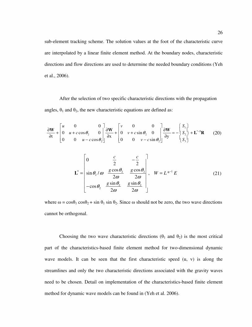
sub-element tracking scheme. The solution values at the foot of the characteristic curve
are interpolated by a linear finite element method. At the boundary nodes, characteristic
directions and flow directions are used to determine the needed boundary conditions (Yeh
et al., 2006).
After the selection of two specific characteristic directions with the propagation
angles, θ1 and θ2, the new characteristic equations are defined as:
1
*
2 2 2
2 2 3
0 0 0 0
0 cos 0 0 sin 0t x y
0 0 cos 0 0 sin
Su v
u c v c S
u c v c S
θ θ
θ θ
−
∂ ∂ ∂ + + + + = − + ∂ ∂ ∂ − −
1W W WL R (20)
12 22
2 22
0 2 2
cos cossin / , *
2 2
sin sincos
2 2
c c
g gW L E
g g
θ θθ ω
ω ω
θ θθ
ω ω
−
−
= = −
*L (21)
where ω = cosθ1 cosθ2 + sin θ1 sin θ2. Since ω should not be zero, the two wave directions
cannot be orthogonal.
Choosing the two wave characteristic directions (θ1 and θ2) is the most critical
part of the characteristics-based finite element method for two-dimensional dynamic
wave models. It can be seen that the first characteristic speed (u, v) is along the
streamlines and only the two characteristic directions associated with the gravity waves
need to be chosen. Detail on implementation of the characteristics-based finite element
method for dynamic wave models can be found in (Yeh et al. 2006).
27
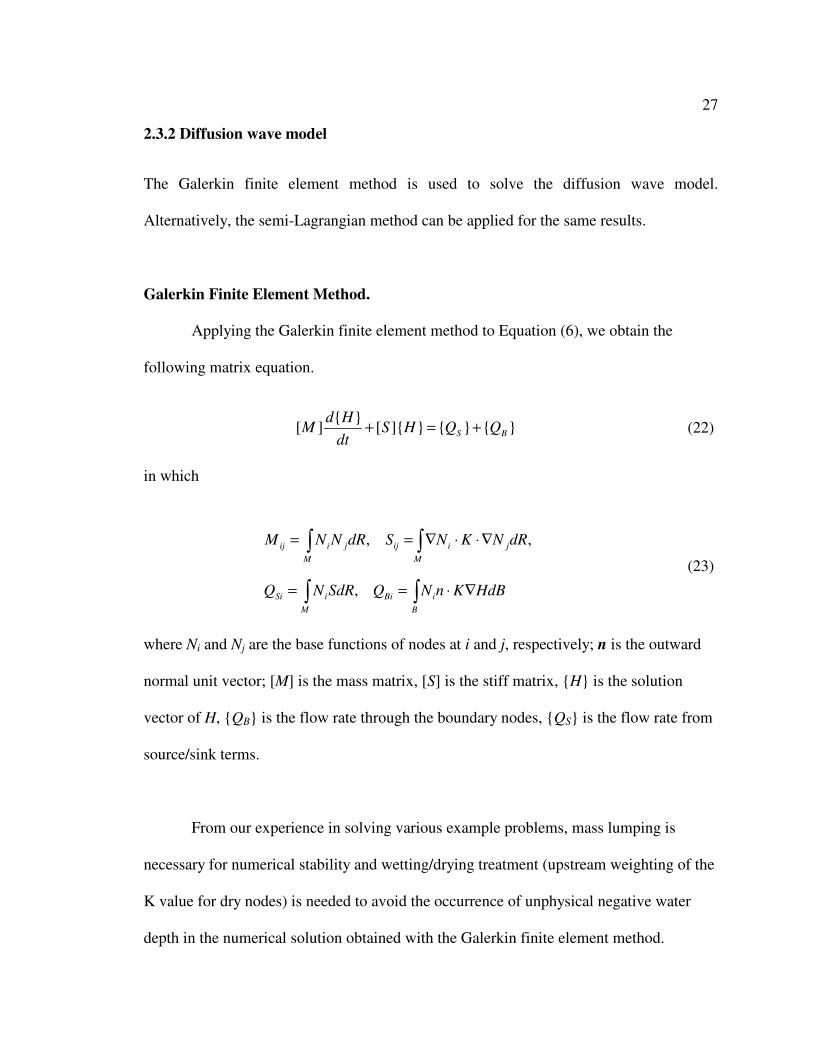
2.3.2 Diffusion wave model
The Galerkin finite element method is used to solve the diffusion wave model.
Alternatively, the semi-Lagrangian method can be applied for the same results.
Galerkin Finite Element Method.
Applying the Galerkin finite element method to Equation (6), we obtain the
following matrix equation.
}{}{}]{[}{
][ BS QQHSdt
HdM +=+ (22)
in which
, ,
,
ij i j ij i j
M M
Si i Bi i
M B
M N N dR S N K N dR
Q N SdR Q N n K HdB
= = ∇ ⋅ ⋅∇
= = ⋅ ∇
∫ ∫
∫ ∫
(23)
where Ni and Nj are the base functions of nodes at i and j, respectively; n is the outward
normal unit vector; [M] is the mass matrix, [S] is the stiff matrix, {H} is the solution
vector of H, {QB} is the flow rate through the boundary nodes, {QS} is the flow rate from
source/sink terms.
From our experience in solving various example problems, mass lumping is
necessary for numerical stability and wetting/drying treatment (upstream weighting of the
K value for dry nodes) is needed to avoid the occurrence of unphysical negative water
depth in the numerical solution obtained with the Galerkin finite element method.
28
Semi-Lagrangian Method.
The Semi-Lagrangian method for diffusion wave model takes the advective form
of the continuity equation and applies a backward particle-tracking scheme to solve for
the unknown variable (water depth). This is described in the following kinematic wave
model section.
For the Semi-Lagrangian approach, wetting/drying can be naturally treated while
mass error control is a major concern.
2.3.3 Kinematic wave model
Since a kinematic wave is purely advective, there is no physical diffusion in the
model. As a result, in the numerical solution of kinematic waves, the numerical diffusion
is a major concern (Ponce, 1989). We apply the semi-Lagrangian method, which is a
natural choice based on the form of the kinematic governing equation. In the hydrologic
modeling literature, the Galerkin finite element methods are used for some kinematic
wave models (for example, Jaber and Mohtar, 2003; Garg and Sen, 2001), although some
stability control was proposed, it is inherently numerically unstable and oscillatory.
For the semi-Lagrangian method, a backward tracking scheme is applied to
solving the kinematic wave equation:
Dh u vS h h
D x yτ
∂ ∂= − −
∂ ∂ (24)
29
Integrating Equation (24) along its characteristic line (u,v) from a new time level
to the foot of characteristics at the previous time level or reaching on the boundary.
2.4 Comparative examples
We will focus on how the incorporation of all three waves - optional dynamic
wave (DYW), diffusion wave (DIW) and kinematic wave (KIW) models can be used to
investigate the applicability and potential errors of simplified DIW and KIW approaches.
From previous studies, it is well known that the accuracy of diffusion and
kinematic wave approximation does not solely depend on bottom slopes, but also rainfall
intensity and duration, boundary conditions, etc. Generalized formal theoretical analyses
are not tractable for two-dimensional flow; numerical experiments are the only way to
investigate the different results obtained by different wave models.
Several numerical tests were conducted to demonstrate the applicability and
accuracy of diffusion or kinematic wave approximation in comparison to the full dynamic
wave solutions. The test examples encompass one-dimensional channel flows with exact
solutions, dam break-type flow, rainfall-induced overland flow and structure flow driven
wetland flow, and two-dimensional river bend flow.
30
2.4.1 Verification and comparison of steady flow in one-dimensional channels
Three channel flow benchmark problems provided by (MacDonald et al., 1997)
were used to verify the numerical schemes implemented for the DYW, DIW, and KIW
and the error of DIW and KIW solutions were discussed.
The one-dimensional channel flow is pure subcritical, subcritical at
inflow/supercritical at outflow, and mixed flow with hydraulic jump, respectively for
Test Problem 1, 2 and 3. The bed slope is given by an analytical function of the pre-
selected water depths. Details on these test problem set-up and the derived exact
analytical solutions can be found in the aforementioned reference.
Test Problem 1: pure subcritical flow
The channel is rectangular with a width of 10 m. The total length is 1,000 m. A
constant flow of 20 m3/s is applied at the upstream end. The flow is pure subcritical. A
water depth of 0.748409 m is specified at the downstream outlet. The Manning’s n value
is 0.03. The bottom slope is given by:
[ ][ ][ ]3/10
3/4
3 )](10
]10)(236.0
)(
41)(
xh
xh
dx
dh
xghxSo
++
−= (25)
which is depicted in Figure 2-4. For this test problem, the analytical solution of the fully
dynamic wave model at steady state is given by MacDonald et al. (1997) as
−−+
=
23/1
2
1
100016exp5.01
4)(
x
gxh (26)
31
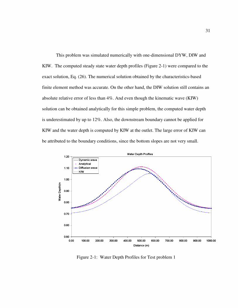
This problem was simulated numerically with one-dimensional DYW, DIW and
KIW. The computed steady state water depth profiles (Figure 2-1) were compared to the
exact solution, Eq. (26). The numerical solution obtained by the characteristics-based
finite element method was accurate. On the other hand, the DIW solution still contains an
absolute relative error of less than 4%. And even though the kinematic wave (KIW)
solution can be obtained analytically for this simple problem, the computed water depth
is underestimated by up to 12%. Also, the downstream boundary cannot be applied for
KIW and the water depth is computed by KIW at the outlet. The large error of KIW can
be attributed to the boundary conditions, since the bottom slopes are not very small.
Figure 2-1: Water Depth Profiles for Test problem 1
32
Test problem 2: Mixed Subcritical/Supercritical Flow:
A rectangular channel of 1,000 m, with a width of 10 m, is given a constant flow rate of
20 m3/s (for the entire channel). The bottom slope is variable and is given as function of x
as
[ ][ ]3/10
3/4
3 )](10
]10)(216.0
)(
41)(
xh
xh
dx
dh
xghxSo
++
−= (27)
The bottom slope given in Eq. (27) would render the flow conditions subcritical at the
inflow boundary and supercritical at the outlet (Figure 2-3). The Manning’s n value is
0.02. This test problem has an exact solution (MacDonald et al. 1997)
≤≤
−−
≤≤
−−
=
10005002
1
10006tanh
6
11
4
50002
1
10003tanh
3
11
4
)(3/1
3/1
xx
g
xx
gxh (28)
For numerical simulations, there is one inflow boundary condition and no
downstream boundary for the dynamic wave model. For diffusive wave model, two
boundary conditions must be given. In this case, the known water depth at outlet was
specified as downstream boundary based on the exact water depth solution given in Eq.
(28).
The dynamic wave model was able to solve this mixed flow problem with good
accuracy. No numerical instabilities have been encountered. The diffusive wave model
also provides satisfactory results (4% error in water depth). The kinematic wave solution
underestimated the water depth by 4% to 6% (Figure 2-2). The Froude number profile
33
plot in Figure 2-3 confirms the mixed flow condition. The bottom slopes range from
0.2% to 0.8%.
Figure 2-2: Water Depth Profiles for Test Problem 2
34
Figure 2-3: Froude Number and bottom slope (%) profiles for Test Problem 2
Figure 2-4: Bottom slope (-) profiles for Test Problems 1 and 3
35
It is interesting to note that even though the dynamic wave model requires less
input data than the diffusive wave model (one boundary condition versus two), it yields
more accurate simulations.
Test problem 3: Mixed Subcritical/Supercritical Flow with Hydraulic Jump
This test problem is described in MacDonald et al. (1997). The channel is
trapezoidal, with a total length of 1,000 m. The upstream inflow is a constant discharge of
20 m3/s. At the downstream outlet, a specified water depth of 1.349963 m was applied.
The side slope of the trapezoidal cross-section is 1:1. The Manning’s n value is 0.02. The
bottom slope is given as function of x as:
[ ][ ]
[ ][ ]3/103/10
3/4
33)()(10
]10)(2216.0
)()(10
)](210[4001)(
xhxh
xh
dx
dh
xhxhg
xhxSo
+
++
+
+−= (29)
which is depicted in Figure 2-4. The exact solution for this problem is (MacDonald et al.
1997)
≤<
−+
−−+
≤≤
−−
≤≤
−−
=
∑=
3
1
100060011000
exp5
3
5
3
100020exp
4
3
60030010
3
10006tanh
6
11723449.0
300010
3
1000tanh1723449.0
)(
k
k xxx
ka
xx
xx
xh (30)
The abrupt change in bed slope (Figure 2-4) causes a hydraulic jump. Both inflow and
outflow boundaries are subcritical.
36
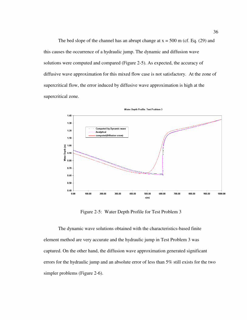
The bed slope of the channel has an abrupt change at x = 500 m (cf. Eq. (29) and
this causes the occurrence of a hydraulic jump. The dynamic and diffusion wave
solutions were computed and compared (Figure 2-5). As expected, the accuracy of
diffusive wave approximation for this mixed flow case is not satisfactory. At the zone of
supercritical flow, the error induced by diffusive wave approximation is high at the
supercritical zone.
Figure 2-5: Water Depth Profile for Test Problem 3
The dynamic wave solutions obtained with the characteristics-based finite
element method are very accurate and the hydraulic jump in Test Problem 3 was
captured. On the other hand, the diffusion wave approximation generated significant
errors for the hydraulic jump and an absolute error of less than 5% still exists for the two
simpler problems (Figure 2-6).
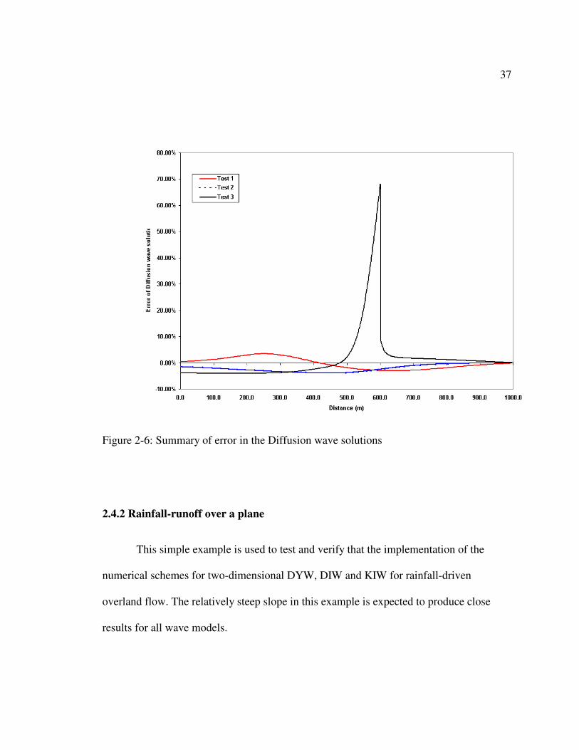
37
Figure 2-6: Summary of error in the Diffusion wave solutions
2.4.2 Rainfall-runoff over a plane
This simple example is used to test and verify that the implementation of the
numerical schemes for two-dimensional DYW, DIW and KIW for rainfall-driven
overland flow. The relatively steep slope in this example is expected to produce close
results for all wave models.
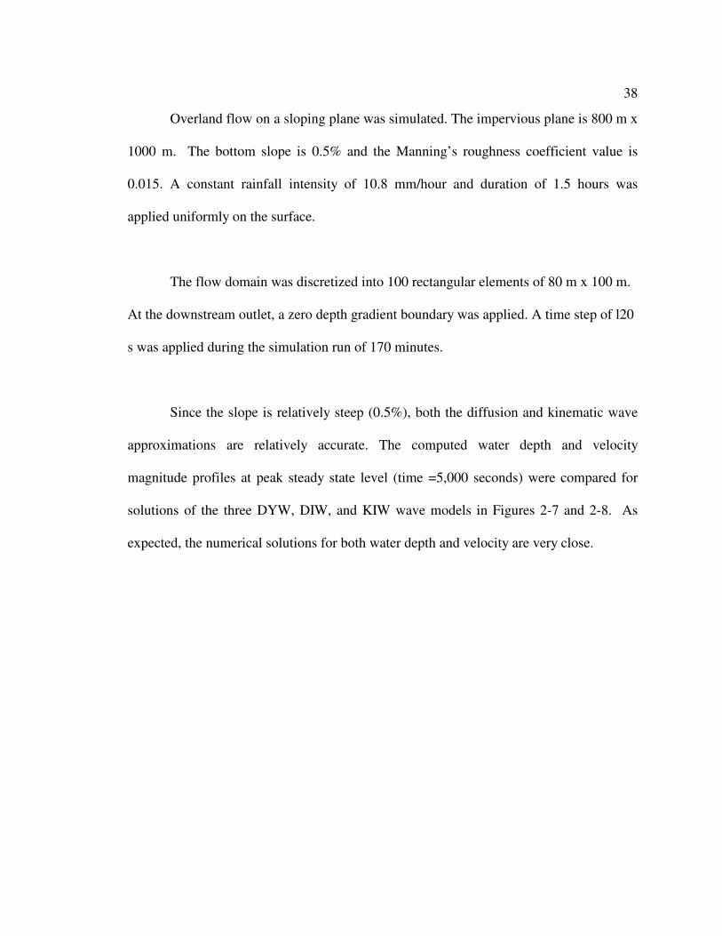
38
Overland flow on a sloping plane was simulated. The impervious plane is 800 m x
1000 m. The bottom slope is 0.5% and the Manning’s roughness coefficient value is
0.015. A constant rainfall intensity of 10.8 mm/hour and duration of 1.5 hours was
applied uniformly on the surface.
The flow domain was discretized into 100 rectangular elements of 80 m x 100 m.
At the downstream outlet, a zero depth gradient boundary was applied. A time step of l20
s was applied during the simulation run of 170 minutes.
Since the slope is relatively steep (0.5%), both the diffusion and kinematic wave
approximations are relatively accurate. The computed water depth and velocity
magnitude profiles at peak steady state level (time =5,000 seconds) were compared for
solutions of the three DYW, DIW, and KIW wave models in Figures 2-7 and 2-8. As
expected, the numerical solutions for both water depth and velocity are very close.
39
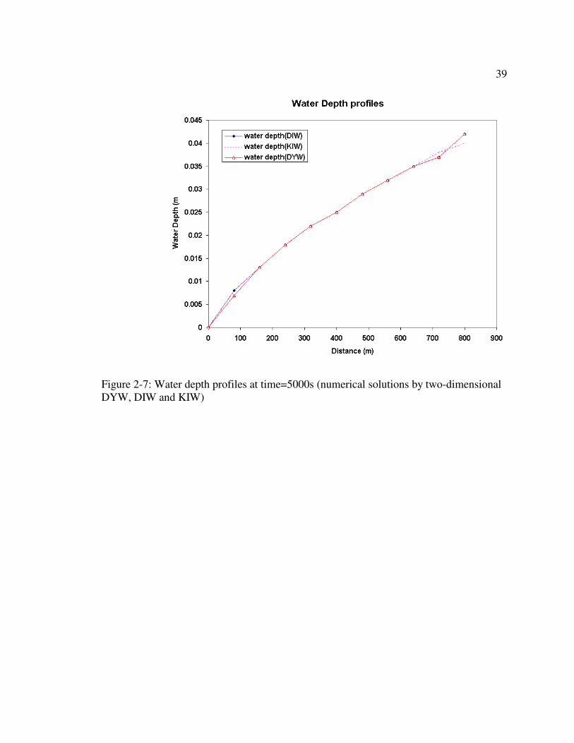
Figure 2-7: Water depth profiles at time=5000s (numerical solutions by two-dimensional
DYW, DIW and KIW)
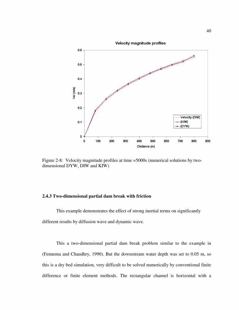
40
Figure 2-8: Velocity magnitude profiles at time =5000s (numerical solutions by two-
dimensional DYW, DIW and KIW)
2.4.3 Two-dimensional partial dam break with friction
This example demonstrates the effect of strong inertial terms on significantly
different results by diffusion wave and dynamic wave.
This a two-dimensional partial dam break problem similar to the example in
(Fennema and Chaudhry, 1990). But the downstream water depth was set to 0.05 m, so
this is a dry bed simulation, very difficult to be solved numerically by conventional finite
difference or finite element methods. The rectangular channel is horizontal with a
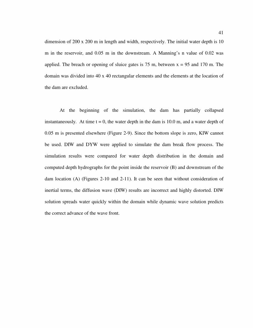
41
dimension of 200 x 200 m in length and width, respectively. The initial water depth is 10
m in the reservoir, and 0.05 m in the downstream. A Manning’s n value of 0.02 was
applied. The breach or opening of sluice gates is 75 m, between x = 95 and 170 m. The
domain was divided into 40 x 40 rectangular elements and the elements at the location of
the dam are excluded.
At the beginning of the simulation, the dam has partially collapsed
instantaneously. At time t = 0, the water depth in the dam is 10.0 m, and a water depth of
0.05 m is presented elsewhere (Figure 2-9). Since the bottom slope is zero, KIW cannot
be used. DIW and DYW were applied to simulate the dam break flow process. The
simulation results were compared for water depth distribution in the domain and
computed depth hydrographs for the point inside the reservoir (B) and downstream of the
dam location (A) (Figures 2-10 and 2-11). It can be seen that without consideration of
inertial terms, the diffusion wave (DIW) results are incorrect and highly distorted. DIW
solution spreads water quickly within the domain while dynamic wave solution predicts
the correct advance of the wave front.
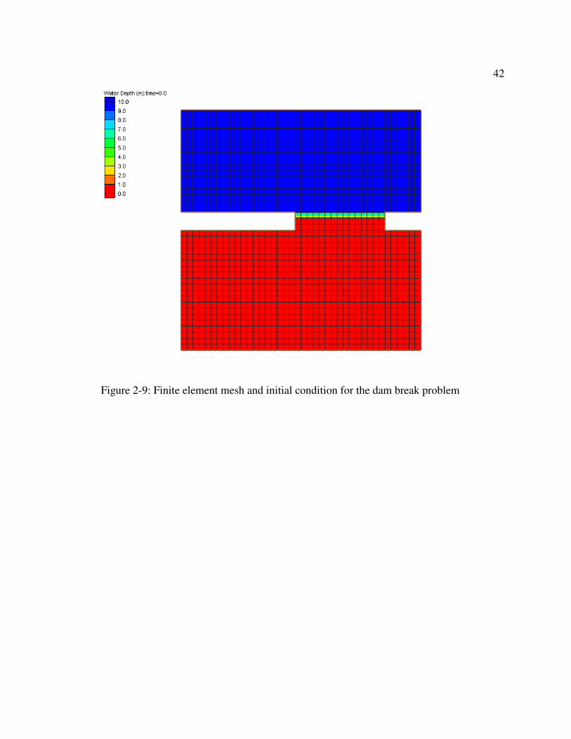
42
Figure 2-9: Finite element mesh and initial condition for the dam break problem
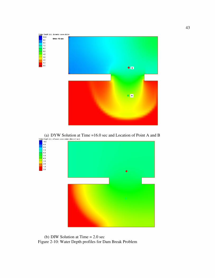
43
(a) DYW Solution at Time =16.0 sec and Location of Point A and B
(b) DIW Solution at Time = 2.0 sec
Figure 2-10: Water Depth profiles for Dam Break Problem
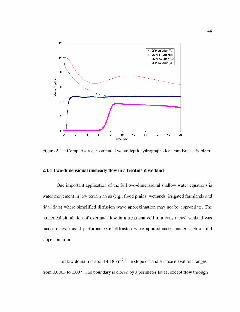
44
Figure 2-11: Comparison of Computed water depth hydrographs for Dam Break Problem
2.4.4 Two-dimensional unsteady flow in a treatment wetland
One important application of the full two-dimensional shallow water equations is
water movement in low terrain areas (e.g., flood plains, wetlands, irrigated farmlands and
tidal flats) where simplified diffusion wave approximation may not be appropriate. The
numerical simulation of overland flow in a treatment cell in a constructed wetland was
made to test model performance of diffusion wave approximation under such a mild
slope condition.
The flow domain is about 4.18 km2. The slope of land surface elevations ranges
from 0.0003 to 0.007. The boundary is closed by a perimeter levee, except flow through
45
the inflow and outflow culverts in the levee (Figures 2-12 and 2-13). There are observed
flow and stage data for this treatment cell and a stage monitoring station is located at the
center of the cell.
Flow during a time period of 240 hours (10 days) was simulated with time-varied
historic flow and stage data (Figure 2-14) and the simulation results of DYW and DIW
were compared. Identical finite element mesh, model parameters and boundary
conditions were used. Both the DYW and DIW solutions were plotted for the water levels
at the observed point with the observed data. Close match (less 0.01 m with water levels
range between 3.80 m to 3.95 m) among the observed, DYW and DIW values were
obtained (Figure 2-15). This example demonstrates that DIW can be applicable to slow
flow on a very mild slope.
For sediment and contaminant transport, accurate velocity calculation is also very
important. There are concerns that flow dynamics cannot be adequately captured by
diffusion wave or kinematic wave approximations. The velocity magnitude and vector
plots also show similar pattern (Figure 2- 16).
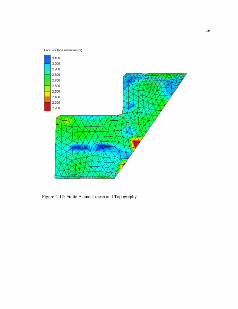
46
Figure 2-12: Finite Element mesh and Topography
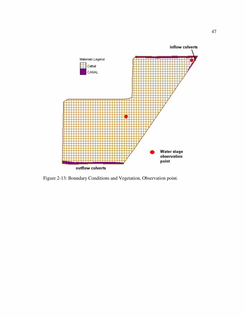
47
Figure 2-13: Boundary Conditions and Vegetation, Observation point.
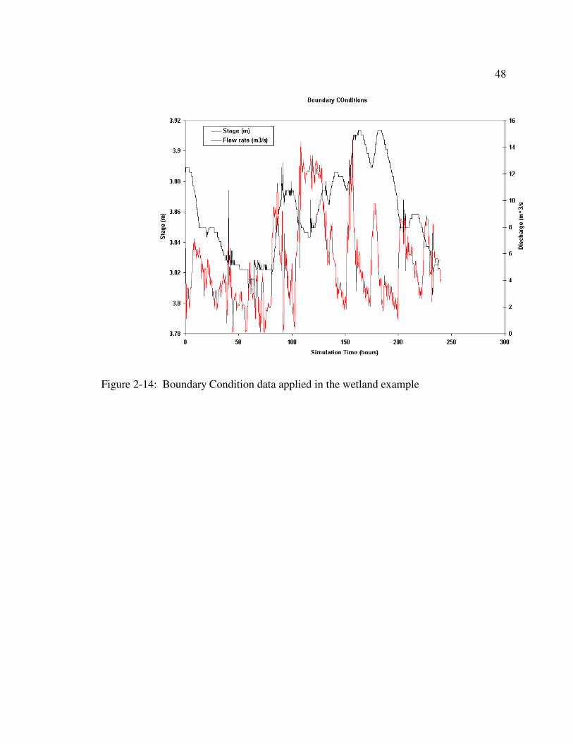
48
Figure 2-14: Boundary Condition data applied in the wetland example
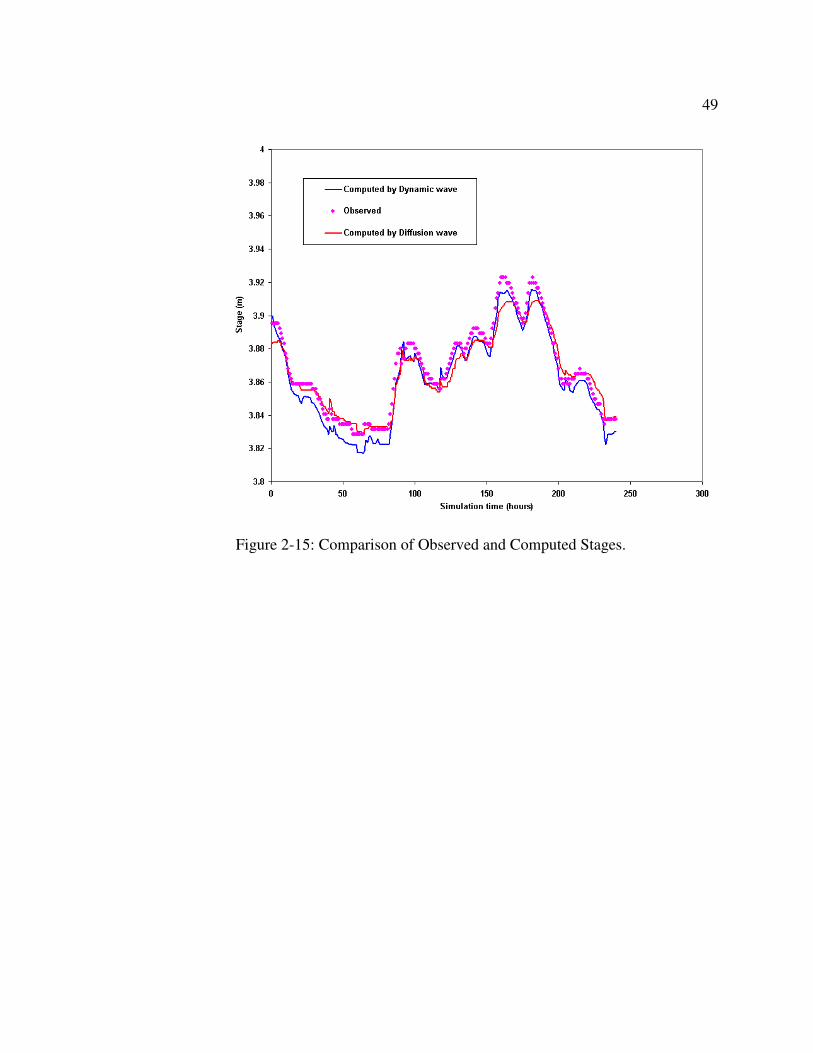
49
Figure 2-15: Comparison of Observed and Computed Stages.
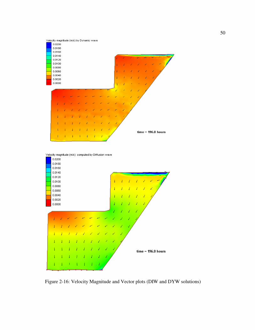
50
Figure 2-16: Velocity Magnitude and Vector plots (DIW and DYW solutions)
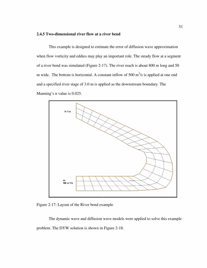
51
2.4.5 Two-dimensional river flow at a river bend
This example is designed to estimate the error of diffusion wave approximation
when flow vorticity and eddies may play an important role. The steady flow at a segment
of a river bend was simulated (Figure 2-17). The river reach is about 800 m long and 50
m wide. The bottom is horizontal. A constant inflow of 500 m3/s is applied at one end
and a specified river stage of 3.0 m is applied as the downstream boundary. The
Manning’s n value is 0.025.
Figure 2-17: Layout of the River bend example
The dynamic wave and diffusion wave models were applied to solve this example
problem. The DYW solution is shown in Figure 2-18.
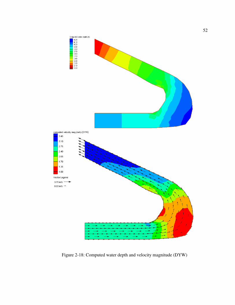
52
Figure 2-18: Computed water depth and velocity magnitude (DYW)
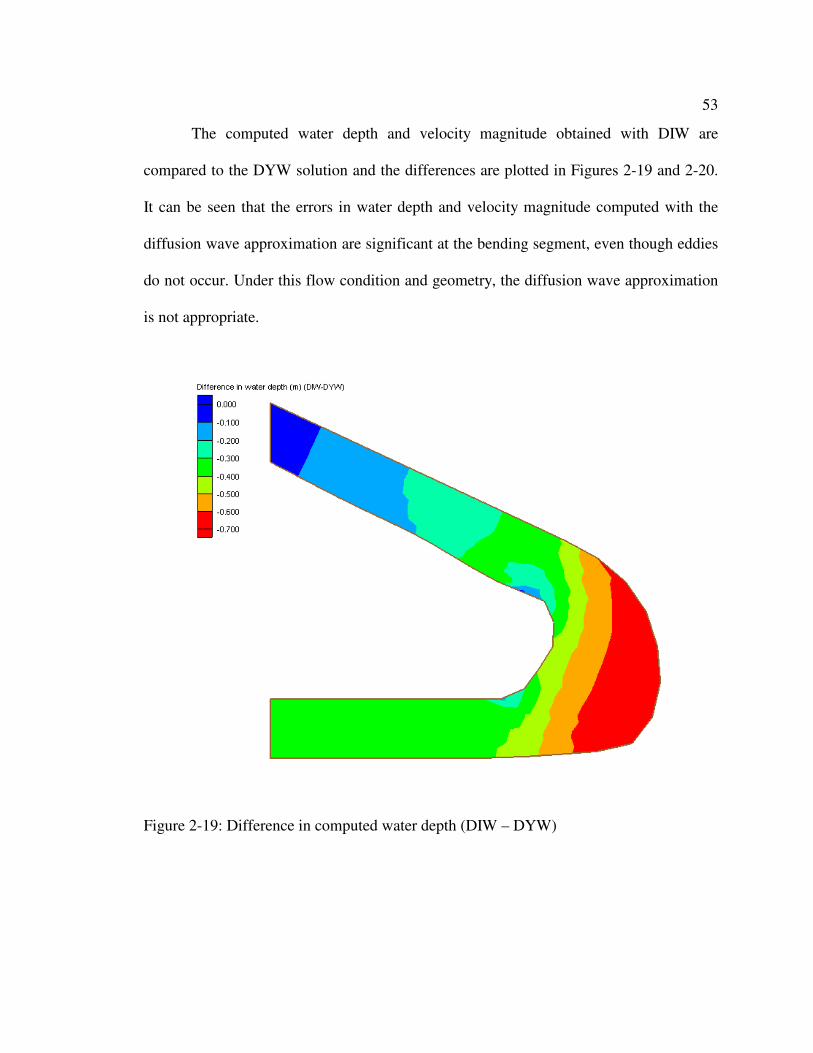
53
The computed water depth and velocity magnitude obtained with DIW are
compared to the DYW solution and the differences are plotted in Figures 2-19 and 2-20.
It can be seen that the errors in water depth and velocity magnitude computed with the
diffusion wave approximation are significant at the bending segment, even though eddies
do not occur. Under this flow condition and geometry, the diffusion wave approximation
is not appropriate.
Figure 2-19: Difference in computed water depth (DIW – DYW)
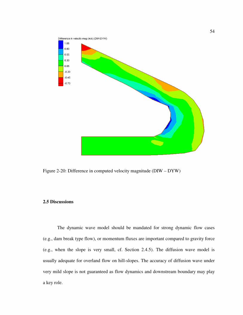
54
Figure 2-20: Difference in computed velocity magnitude (DIW – DYW)
2.5 Discussions
The dynamic wave model should be mandated for strong dynamic flow cases
(e.g., dam break type flow), or momentum fluxes are important compared to gravity force
(e.g., when the slope is very small, cf. Section 2.4.5). The diffusion wave model is
usually adequate for overland flow on hill-slopes. The accuracy of diffusion wave under
very mild slope is not guaranteed as flow dynamics and downstream boundary may play
a key role.
55
The kinematic wave model is still popular in many watershed models. It should be
limited though, specifically to steep-slope mountainous watersheds and where
downstream conditions are not important. Instead of this method, an adaptive scheme for
applying DYW, DIW, or KIW in different sub-domains of a watershed may prove to be
more efficient and therefore advantageous.
2.6 Summary and Conclusions
The implementation of dynamic wave, diffusion wave, and kinematic wave
models in a single watershed model is an advantage in order to strongly validate the
derived approximations. This is illustrated by some numerical examples that demonstrate
the potential errors in diffusion wave and kinematic wave models for overland flow.
Acknowledgements
This research is supported by the U.S. EPA - Science To Achieve Results (STAR)
Program under Grant # R-82795602 with the University of Central Florida.
56
References
Donigian, A.S. and J. Imhoff. (2006). Chapter 2: History and evolution of watershed
modeling derived from the Stanford Watershed model, in Watershed Models. Eds. By
Singh VP and Frevert, CRC Press, Boca Raton, FL.
Fennema R.J. and M.H. Chaudhry (1990). Explicit methods for 2-D transient free-surface
flows, Journal of Hydraulic Engineering, Vol. 116, No.8, pp.1012-1033, 1990.
Fortin, J. P., Turcotte, R., Massicotte, S., Moussa, R., Fitzback, J., and Villeneuve, J. P.
(2001). ‘‘A distributed watershed model compatible with remote sensing and GIS data.
I: Description of model.’’ J. Hydrologic Eng., 6(2), 91–99.
Govindaraju, R. S., Jones, S. E., and Kavvas, M. L. (1988). ‘On the diffusion wave
model for overland flow: 2. Steady state analysis’, Water Resources Research, 24, 745-
754.
Govindaraju, R.S., Kavvas, M.L. and Jones, S.E. (1990). 'Approximate analytical
solutions for overland flows.' Water Resources Research, 26(12), pp. 2903-2912.
57
Hydrologic Engineering Center(HEC). (2000). ‘‘Hydrologic modeling system HEC-
HMS user’s manual, version 2.’’ Engineering, U.S. Army Corps of Engineers, Davis,
Calif.
Maconald I., Baines, M.J., Nichols N.K. and Samuels P.G. (1997). Analytic Benchmark
Solutions for Open Channel Flows, Journal of Hydraulic Engineering, Vol. 123, No.
11, November, 1997.
Metcalf and Eddy, Inc., Univ. of Florida, and Water Resources Engineers, Inc. (1971).
‘‘Storm water management model, Vol. 1—Final report.’’ EPA Rep. No.
11024DOC07/71 (NITS PB-203289), EPA, Washington, D.C.
Moramarco1 T. and Singh V.P., (2002). Accuracy of kinematic wave and diffusion wave
for spatial-varying rainfall excess over a plane. Hydrol. Process. 16, 3419–3435.
Jaber F.H. and Mohtar R.H., (2003). Stability and accuracy of two-dimensional kinematic
wave overland flow modeling, Advances in Water Resources 26 (2003) 1189–1198.
Olivera, F., and Maidment, D. (1999). ‘‘Geographical information system ~GIS!-based
spatially distributed model for runoff routing.’’ Water Resour. Res., 35(4), 1155–1164.
58
Parlange, J. Y., Hogarth, W., Sander, G., Rose, C., Haverkamp, R., Surin, A., and
Brutsaert, W. (1990). ‘Asymptotic expansion for steady state overland flow’, Water
Resources Research, 26, 579-583.
Ponce, V.M., R.M. Li, and D.B. Simons, (1978). Applicability of kinematic and diffusion
wave models. Journal of the Hydraulics Division, ASCE, 104: 353-360.
Richardson, J.R. and P.Y. Julien (1994). 'Suitability of simplified overland flow
equations.' Water Resources Research, 30 (3), pp. 665-671.
Singh VP, Aravamuthan V. (1995). Accuracy of kinematic wave and diffusion wave
approximations for time-independent flows. Hydrological Processes 9: 755–782.
Singh, V.P., S. K. Jain and M. M. Sherif, (2005). Errors of kinematic wave and diffusion
wave approximations for time-independent flows with infiltration and momentum
exchange included, Hydrol. Process. 19, 1771–1790.
Tayfur, G., Kavvas, M. L., Govindaraju, R. S., and Storm, D. E., (1993), ‘‘Applicability
of St. Venant equations for two dimensional overland flows overrough infiltrating
surfaces.’’ J. Hydraul. Eng., 119(1), 51–63.
Yeh, G.T., G. B. Huang, H. P. Cheng, F. Zhang, H. C. Lin, E. Edris, and D. Richards.
(2006). A first principle, physics-based watershed model: WASH123D, in Watershed

59
Models. Eds. By Singh VP and Frevert D.K., CRC Press, Boca Raton, FL, September
2005.
60
Chapter 3
Dynamic Wave Modeling of Two-dimensional Overland Flow using Characteristics-
based Finite Element Method
Abstract
The Method of Characteristics (MOC), within the context of the finite element
method, was applied to the complete two-dimensional shallow water equations for two-
dimensional overland flow. For two-dimensional overland flow, finite element or finite
volume methods are more flexible in dealing with complex boundary. Recently, finite
volume methods have been very popular in numerical solution of the shallow water
equations. Some (e.g., Hirsch et al, 1987; Garcia-Navarro et al., 1995 and Guinot, 2004)
have pointed out that finite volume methods for two-dimensional flow are fundamentally
one-dimensional (normal to the cell interface). The results may rely on the grid
orientation. The search for genuinely multidimensional numerical schemes for two-
dimensional flow is an active topic. We consider the Method of Characteristics (MOC)
in the context of finite element method as a good alternative. Many researchers (e.g.,
Zhang and Cundy, 1989; Chow and Ben-Zvi, 1973 and Katopodes and Strelkoff, 1979)
have pointed out the advantage of MOC in solving two-dimensional shallow water
hyperbolic equations having wave-like solutions. At the same time, they considered
MOC for two-dimensional overland flow being non-tractable on complex topography.
The intrinsic difficulty in implementing MOC for two-dimensional overland flow is that
there are infinite numbers of wave characteristics in the two-dimensional context,
61
although only three independent wave directions are needed for a well-posed solution to
the characteristic equations. We have implemented a numerical scheme that attempts to
diagonalize the characteristic equations based on a pressure and velocity-gradient
relationship. This new scheme was evaluated by comparison with other choices of wave
characteristic directions, given in the literature. Example problems of mixed sub-critical
flow/super-critical flow in a channel, with approximate analytical solutions, were used to
verify the numerical algorithm. Then experiments of overland flow on a cascade of three
planes (Iwagaki, 1955) were solved with the new method. The circular dam break
problem was solved with different selections of wave characteristic directions, and the
performance of each selection was evaluated based on accuracy and numerical stability.
Finally, two-dimensional overland flow over complex topography in a wetland setting,
with very mild slope, was solved with the new numerical method to demonstrate its
applicability.
3.1 Introduction
The simplified form of the two-dimensional shallow water equations (e.g. the
diffusion wave or kinematic wave approximation) has been frequently used in modeling
the two-dimensional shallow overland flow originated from the rainfall/runoff process,
surface flow in irrigation and wetlands, and flooding in floodplains. On the other hand,
the full two-dimensional shallow water equations have been extensively studied for fast
transient flow processes (dam break type flood propagation and hydraulic jumps) or deep
surface water flows in estuary and ocean.
62
The characteristics of overland flow in comparison to deep surface water flow can
be summarized as (e.g. Zhang and Cundy, 1989): (1) very small water depth; (2) large
bed shear stress; (3) impact of grid scale micro-topography; (4) stiff source term induced
by rainfall and infiltration; and, (5) dynamically wetting and drying boundary. The full
two-dimensional shallow water equations are the most appropriate for capturing all these
complex overland flow features.
Chow and Ben-Zvi (1973) reported the first two-dimensional hydrodynamic
model for overland flow using the Lax-Wendroff scheme. Zhang and Cundy (1989)
applied the explicit MaCormack finite difference scheme for two-dimensional overland
flow. Fielder and Ramirez (2000) also applied the explicit MaCormack scheme with
some special treatment of the advection and source terms for two-dimensional overland
shallow water equations. Simulation of overland flow at plot size at the scale of 1 ~ 10 m2
was reported in these studies. These classical methods and some other central difference
schemes are prone to numerical instabilities and special treatments are required to
achieve a stable and convergent numerical solution. Zhao et al. (1994) developed a
finite volume model for two-dimensional surface water flow. Finite volume methods
combined with shock capturing scheme have been very popular and seem successful for
the homogeneous shallow water equations. However, finite volume methods are
intrinsically one-dimensional (normal to the cell interfaces) and the manipulation of
source terms is difficult and complicated for higher order schemes. In the finite
63
difference context, the classical method of characteristics has been considered to be
advantageous in solving the two-dimensional shallow water equations for overland flow,
but it is also thought to be extremely difficult and not tractable for the general overland
flow case of complex topography and variability (Chow and Ben-Zvi, 1973; Zhang and
Cundy, 1989). Katopodes and Strelkoff (1978; 1979) developed a numerical scheme
based on the method of characteristics in the framework of finite difference method for
two-dimensional dam break simulations.
In the finite element framework, it is well known that Galerkin finite element
methods perform very poorly for advection-dominant shallow water flows. The
streamline upwind finite element methods (SUPG) apply selective dissipation to dampen
numerical oscillation (Katopodes, 1984). Lately, the discontinuous Galerkin finite
element method has also been applied for trans-critical shallow water flows
(Schwanenberg and harms, 2004).
All above-mentioned methods are Eulerian with some stabilization schemes.
Since the shallow water equations are partial differential equations of hyperbolic type,
characteristics-based or Eulerian-Largragian methods are more appropriate. The
characteristic Galerkin method (Zienkiewicz et al., 1999) was developed for the scalar
advection equation, but is not directly applicable to the shallow water equations because
more than one characteristic speeds are involved. The characteristic-based split (CBS)
scheme was proposed to resolve this difficulty. Paillere et al. (1998), Brufau and Garcia-
64
Navarro (2003) and Garcia-Navarro et al. (1995) studied genuinely multidimensional
upwinding schemes for the 2D shallow water equations based on a residual distribution
scheme with wave models. Guinot (2005) studied approximate two-dimensional Riemann
solver for hyperbolic systems of conservation laws in the framework of finite volume
methods. They applied the new scheme for dam break problems and demonstrated the
improvement in the numerical solutions by a two-dimensional approach for computing
the numerical flux in finite volume methods.
In this paper, we present the classical Method of Characteristics (MOC) in the
context of finite element methods in the Eulerian-Lagrangian framework; the intrinsic
difficulty in two-dimensional MOC methods for two-dimensional shallow water
equations is that there are infinite characteristic wave directions to choose from, although
there are only three independent wave directions. Hirsch et al. (1987) proposed a
diagonalization approach for the multidimensional Euler equations. It is well known that
the shallow water equations are analogous to the Euler equations for gas dynamics. Thus,
a similar diagonlalization was implemented for the shallow water equations in the
framework of finite element in the current study. The characteristic decomposition model
used by Paillere et al. (1998) was also tested for better stability for sub-critical flow.
Numerical schemes based on different combinations of characteristic wave directions
were evaluated using typical overland flow examples. The numerical experiments on
frictionless circular dam break problem, rainfall-runoff over complex surface, wetland
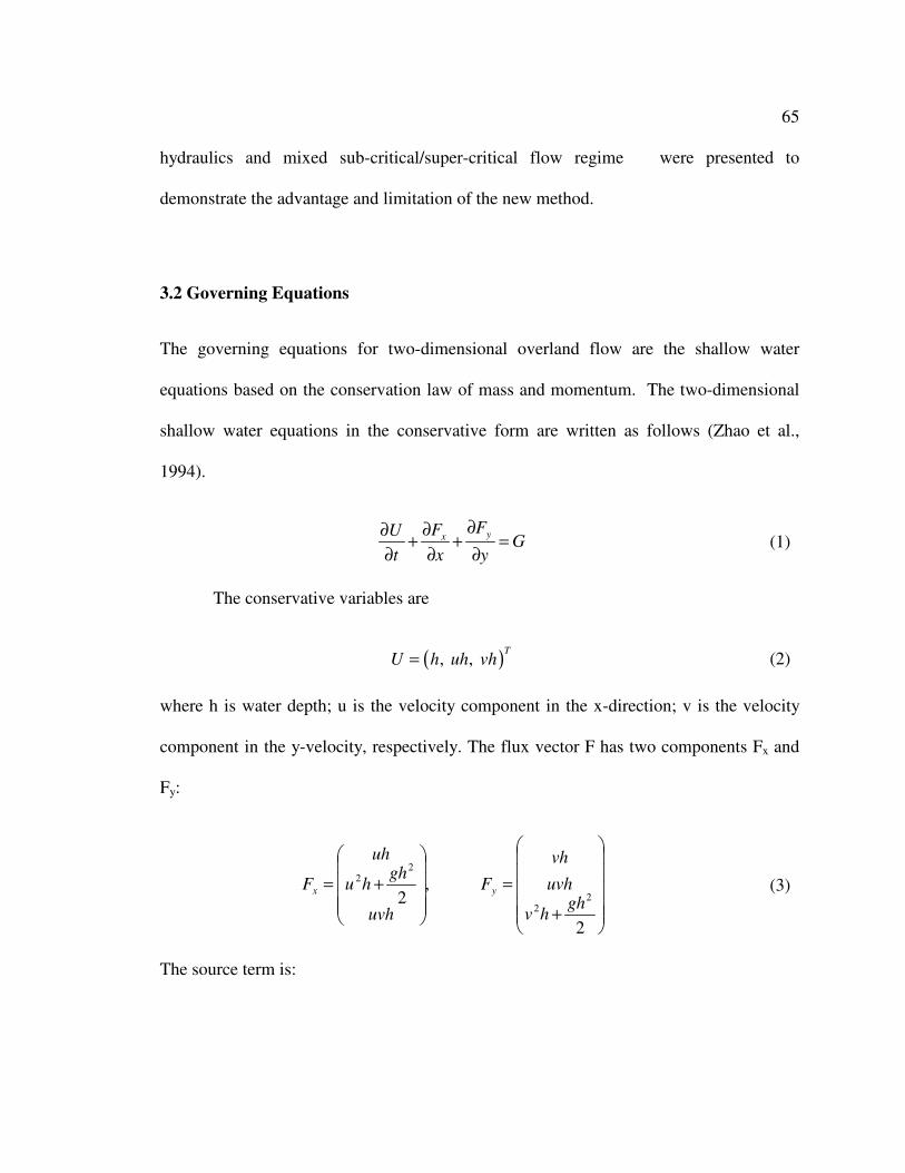
65
hydraulics and mixed sub-critical/super-critical flow regime were presented to
demonstrate the advantage and limitation of the new method.
3.2 Governing Equations
The governing equations for two-dimensional overland flow are the shallow water
equations based on the conservation law of mass and momentum. The two-dimensional
shallow water equations in the conservative form are written as follows (Zhao et al.,
1994).
Gy
F
x
F
t
U yx =∂
∂+
∂
∂+
∂
∂ (1)
The conservative variables are
( ), , T
U h uh vh= (2)
where h is water depth; u is the velocity component in the x-direction; v is the velocity
component in the y-velocity, respectively. The flux vector F has two components Fx and
Fy:
+
=
+=
2
,2 2
2
22
ghhv
uvh
vh
F
uvh
ghhu
uh
F yx (3)
The source term is:
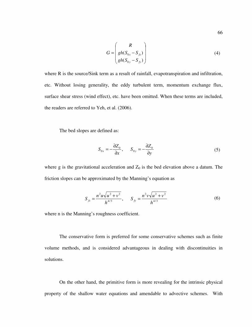
66
−
−=
)(
)(
0
0
fyy
fxx
SSgh
SSgh
R
G (4)
where R is the source/Sink term as a result of rainfall, evapotranspiration and infiltration,
etc. Without losing generality, the eddy turbulent term, momentum exchange flux,
surface shear stress (wind effect), etc. have been omitted. When these terms are included,
the readers are referred to Yeh, et al. (2006).
The bed slopes are defined as:
y
ZS
x
ZS yx
∂
∂−=
∂
∂−= 0
00
0 , (5)
where g is the gravitational acceleration and Z0 is the bed elevation above a datum. The
friction slopes can be approximated by the Manning’s equation as
3/4
222
3/4
222
,h
vuvnS
h
vuunS fyfx
+=
+= (6)
where n is the Manning’s roughness coefficient.
The conservative form is preferred for some conservative schemes such as finite
volume methods, and is considered advantageous in dealing with discontinuities in
solutions.
On the other hand, the primitive form is more revealing for the intrinsic physical
property of the shallow water equations and amendable to advective schemes. With
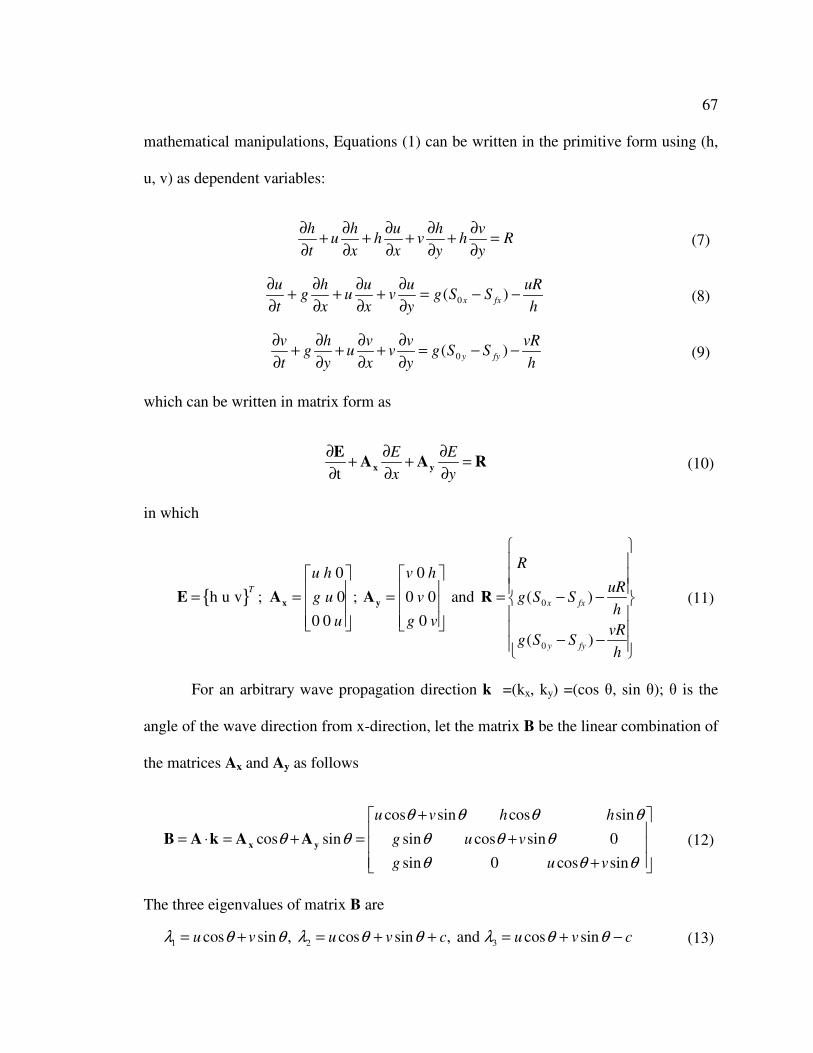
67
mathematical manipulations, Equations (1) can be written in the primitive form using (h,
u, v) as dependent variables:
Ry
vh
y
hv
x
uh
x
hu
t
h=
∂
∂+
∂
∂+
∂
∂+
∂
∂+
∂
∂ (7)
h
uRSSg
y
uv
x
uu
x
hg
t
ufxx −−=
∂
∂+
∂
∂+
∂
∂+
∂
∂)( 0 (8)
h
vRSSg
y
vv
x
vu
y
hg
t
vfyy −−=
∂
∂+
∂
∂+
∂
∂+
∂
∂)( 0 (9)
which can be written in matrix form as
RAAE
yx =∂
∂+
∂
∂+
∂
∂
y
E
x
E
t (10)
in which
{ }
0 0
h u v ; 0 ; 0 0
0 0 0
T
u h v h
g u v
u g v
= = =
x yE A A and
−−
−−=
h
vRSSg
h
uRSSg
R
fyy
fxx
)(
)(
0
0R (11)
For an arbitrary wave propagation direction k =(kx, ky) =(cos θ, sin θ); θ is the
angle of the wave direction from x-direction, let the matrix B be the linear combination of
the matrices Ax and Ay as follows
+
+
+
=+=⋅=
θθθ
θθθ
θθθθ
θθ
sincos0sin
0sincossin
sincossincos
sincos
vug
vug
hhvu
yx AAkAB (12)
The three eigenvalues of matrix B are
1 2 3cos sin , cos sin , and cos sinu v u v c u v cλ θ θ λ θ θ λ θ θ= + = + + = + − (13)
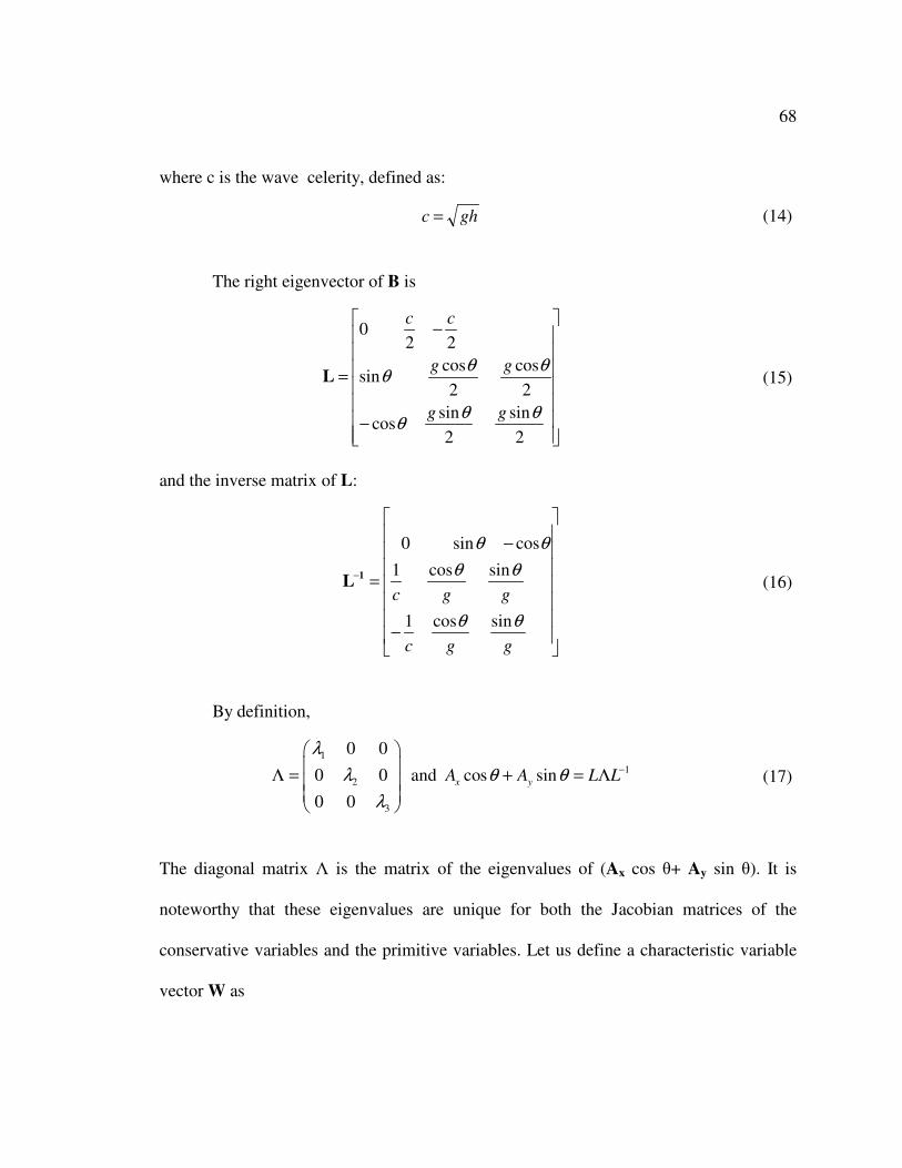
68
where c is the wave celerity, defined as:
ghc = (14)
The right eigenvector of B is
−
−
=
2
sin
2
sincos
2
cos
2
cossin
220
θθθ
θθθ
gg
gg
cc
L (15)
and the inverse matrix of L:
−
−
=−
ggc
ggc
θθ
θθ
θθ
sincos1
sincos1
cossin0
1L (16)
By definition,
1
1
2
3
0 0
0 0 and cos sin
0 0
x yA A L L
λ
λ θ θ
λ
−
Λ = + = Λ
(17)
The diagonal matrix Λ is the matrix of the eigenvalues of (Ax cos θ+ Ay sin θ). It is
noteworthy that these eigenvalues are unique for both the Jacobian matrices of the
conservative variables and the primitive variables. Let us define a characteristic variable
vector W as
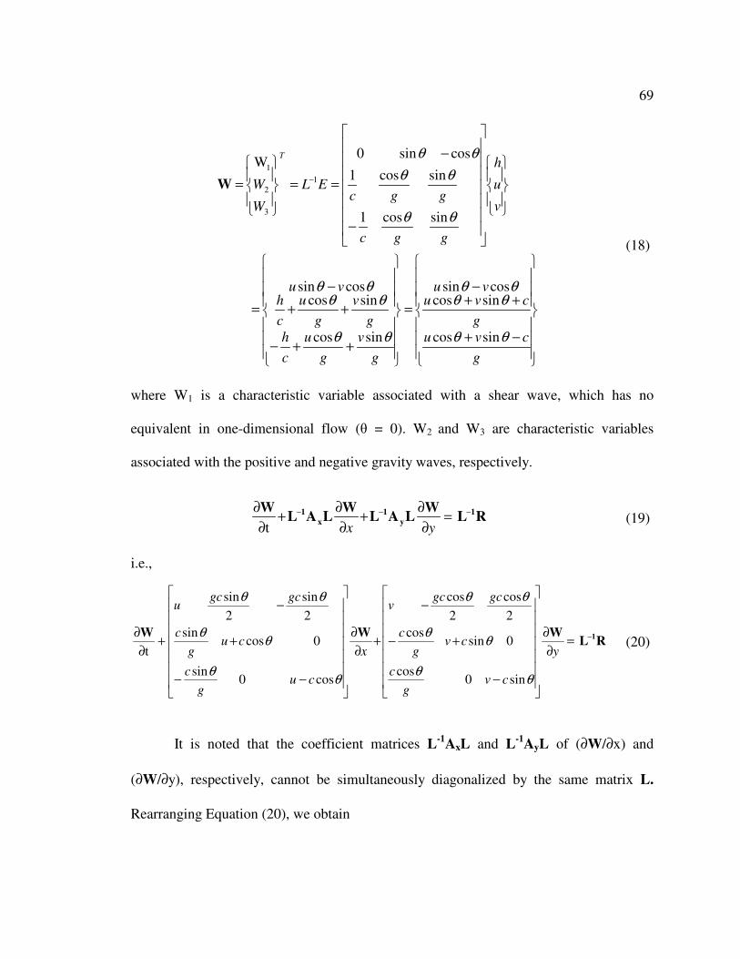
69
−+
++−
=
++−
++
−
=
−
−
==
= −
g
cvu
g
cvuvu
g
v
g
u
c
h
g
v
g
u
c
hvu
v
u
h
ggc
ggcEL
W
W
T
θθ
θθθθ
θθ
θθθθ
θθ
θθ
θθ
sincos
sincoscossin
sincos
sincoscossin
sincos1
sincos1
cossin0W
1
3
2
1
W
(18)
where W1 is a characteristic variable associated with a shear wave, which has no
equivalent in one-dimensional flow (θ = 0). W2 and W3 are characteristic variables
associated with the positive and negative gravity waves, respectively.
RLW
LALW
LALW 1
y
1
x
1 −−− =∂
∂+
∂
∂+
∂
∂
yxt (19)
i.e.,
RLWWW 1−=∂
∂
−
+−
−
+∂
∂
−−
+
−
+∂
∂
y
cvg
c
cvg
c
gcgcv
x
cug
c
cug
c
gcgcu
θθ
θθ
θθ
θθ
θθ
θθ
sin0cos
0sincos
2
cos
2
cos
cos0sin
0cossin
2
sin
2
sin
t
(20)
It is noted that the coefficient matrices L-1
AxL and L-1
AyL of (∂W/∂x) and
(∂W/∂y), respectively, cannot be simultaneously diagonalized by the same matrix L.
Rearranging Equation (20), we obtain
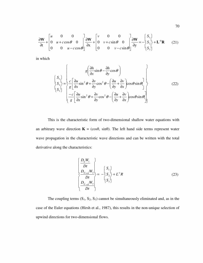
70
RLWWW 1−+
−=∂
∂
−
++∂
∂
−
++∂
∂
3
2
1
ysin00
0sin0
00
xcos00
0cos0
00
tS
S
S
cv
cv
v
cu
cu
u
θ
θ
θ
θ (21)
in which
∂
∂+
∂
∂−
∂
∂+
∂
∂−
∂
∂+
∂
∂−
∂
∂+
∂
∂
∂
∂−
∂
∂
=
θθθθ
θθθθ
θθ
sincoscossin
sincoscossin
cossin
22
22
3
2
1
x
v
y
u
y
v
x
u
g
c
x
v
y
u
y
v
x
u
g
c
y
h
x
hg
S
S
S
(22)
This is the characteristic form of two-dimensional shallow water equations with
an arbitrary wave direction K = (cosθ, sinθ). The left hand side terms represent water
wave propagation in the characteristic wave directions and can be written with the total
derivative along the characteristics:
RL
S
S
S
Dt
WD
Dt
WD
Dt
WD
kcV
kcV
V
1
3
2
1
3
2
1
−
−
+ +
−=
rr
rr
r
(23)
The coupling terms (S1, S2, S3) cannot be simultaneously eliminated and, as in the
case of the Euler equations (Hirsh et al., 1987), this results in the non-unique selection of
upwind directions for two-dimensional flows.
71
It is noteworthy that the above characteristic equations in Lagrangian form,
Equation (23), are identical to both the original conservative and primitive forms of the
shallow water equations. No numerical approximations have been introduced.
The governing equations must be supplemented with initial condition and
appropriate boundary conditions for a well-posed two-dimensional overland flow
problem. Wave characteristic directions at the boundary determine the required boundary
conditions. For example, at an inflow boundary, if flow is subcritical, both shear wave
traveling along the streamline and the positive gravity wave along the normal into the
flow domain, so two boundary conditions have to be imposed.
3.3 Numerical Methods
The Eulerian-Lagrangian method (ELM) is a popular framework for the
numerical solution of the scalar advection-diffusion transport equation. This can be
extended to the solution of advection dominant flow equations. In the case of two-
dimensional shallow water equations, the advection of shear wave and gravity wave
properties in the space-time domain can be decoupled into three convective equations
with source terms, as shown in Equation (23).
After the selection of two specific characteristic directions with the propagation
angles, θ1 and θ2, new characteristic variables are defined as
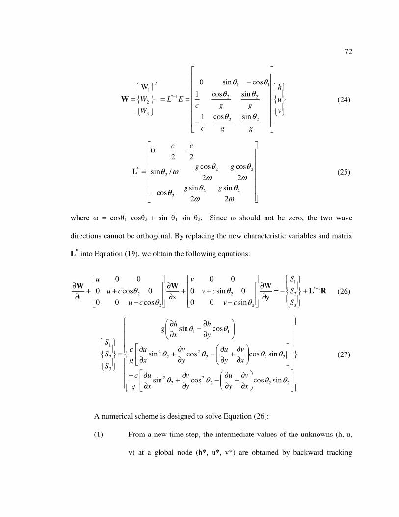
72
−
−
==
= −
v
u
h
ggc
ggcEL
W
W
T
22
22
11
1*
3
2
1
sincos1
sincos1
cossin0W
θθ
θθ
θθ
W (24)
−
−
=
ω
θ
ω
θθ
ω
θ
ω
θωθ
2
sin
2
sincos
2
cos
2
cos/sin
220
222
222
gg
gg
cc
*L (25)
where ω = cosθ1 cosθ2 + sin θ1 sin θ2. Since ω should not be zero, the two wave
directions cannot be orthogonal. By replacing the new characteristic variables and matrix
L* into Equation (19), we obtain the following equations:
RLWWW 1−+
−=∂
∂
−
++∂
∂
−
++∂
∂ *
3
2
1
2
2
2
2y
sin00
0sin0
00
xcos00
0cos0
00
tS
S
S
cv
cv
v
cu
cu
u
θ
θ
θ
θ (26)
∂
∂+
∂
∂−
∂
∂+
∂
∂−
∂
∂+
∂
∂−
∂
∂+
∂
∂
∂
∂−
∂
∂
=
222
2
2
2
222
2
2
2
11
3
2
1
sincoscossin
sincoscossin
cossin
θθθθ
θθθθ
θθ
x
v
y
u
y
v
x
u
g
c
x
v
y
u
y
v
x
u
g
c
y
h
x
hg
S
S
S
(27)
A numerical scheme is designed to solve Equation (26):
(1) From a new time step, the intermediate values of the unknowns (h, u,
v) at a global node (h*, u*, v*) are obtained by backward tracking
73
along the characteristics until the foot of the characteristics at the old
time step is reached or a boundary is hit.
(2) The final numerical solutions are obtained by integrating the RHS
terms along the characteristic lines with a simple trapezoidal
integration rule.
3.3.1 Backward Tracking approach
In the finite element context, the backward tracking scheme is a sub-element-
tracking scheme developed by Cheng et al. (1996) and improved by Suk (2003). The
solution values at the foot of the characteristic curve are interpolated by linear finite
elements.
3.3.2 Characteristic wave directions
Choosing the two wave characteristic directions (θ1 and θ2) is the most critical
part of the characteristics-based finite element method. It can be seen that the first
characteristic speed (u, v) is along the streamlines and only the two characteristic
directions associated with the gravity waves need to be chosen.
The first approach is the wave directions based on maximum diagonalization: The first
choice is based on the minimization of the coupling term (Equation (27)). This follows
the diagonalization approach for the Euler equations suggested by Hirsh et al. (1987). By
setting the coupling terms to zero, we have the following relationships.

74
1 1
2 2
2 2 2 2
2 2
2 2 2 2
sin cos 0,
sin cos cos sin 0,
sin cos cos sin 0
h hg
x y
c u v u v
g x y y x
c u v u v
g x y y x
θ θ
θ θ θ θ
θ θ θ θ
∂ ∂− =
∂ ∂
∂ ∂ ∂ ∂+ − + =
∂ ∂ ∂ ∂
− ∂ ∂ ∂ ∂+ − + =
∂ ∂ ∂ ∂
(28)
From the above algebraic equations, we observe that the first characteristic direction is
related to the shear wave and the two gravity waves share the same second characteristic
direction.
The first characteristic direction is determined by
xh
yh
∂∂
∂∂=
/
/tan 1θ (29)
which is in the pressure gradient direction.
The second characteristic direction, if one exists, is based on the solution of the
following equation:
0sincoscossin 222
2
2
2 =
∂
∂+
∂
∂−
∂
∂+
∂
∂θθθθ
x
v
y
u
y
v
x
u (30)
Equation (30) can have two, one, or no solutions. If no solutions can be found, the
following particular characteristic direction as suggested in Roe (1986) for the treatment
of the Euler equations will be used
yvxu
xvyu
∂∂−∂∂
∂∂+∂∂=
//
//tan 2θ (31)
75
If one solution can be found, it is used in computing θ2. If two real solution can be found,
the one that maximizes ω = cosθ1 cosθ2 + sin θ1 sin θ2 will be used.
It is noteworthy that by choosing wave decomposition following the flow gradients
(depth and velocity), it may be possible to minimize the coupling terms and obtain
diagonalization of the shallow water equations. However, numerical experiments show
that this approach often suffer from convergence problem (e.g., Paillere et al., 1998). The
characteristic directions are dependent on the numerical solution and sensitive to the
accurate evaluation of the gradients of water depth and velocity components. Numerical
stability and convergence are the major concern.
The second approach is the characteristic decomposition: Proposed by Paillere et al.,
1998, when the flow is supercritical, the angle θ2 is taken to be along the Froude line as
2
1sin
Frθ = (32)
where Fr is the Froude number defined as (Fr2 = (u
2+v
2)/c
2). If the flow is subcritical, the
propagation angle is taken as
22
1
1tan
Fr−=θ (33)
The first characteristic direction θ1 is chosen to be equal to the angle θ2 in order to
maximize the determinant of the transformation (ω = 1.0).

76
The coupling terms will not be zero with this selection of characteristic directions.
On the other hand, numerical experiments show that this approach is more stable.
The last approach is the ad-hoc wave directions based on some geometric parameters:
The first characteristic direction can always be selected in the depth gradient direction.
The second characteristic directions can be chosen arbitrary, for example, along the x-
direction, the y-direction or the steepest elevation gradients. This approach is less
accurate and grid orientation of the numerical solutions may occur.
3.4 Verification and Validation Examples
3.4.1 Example 1: non-uniform steady flow in a straight channel
This is a nontrivial channel flow benchmark problem reported by (MacDonald et
al., 1997) to verify and test the performance of numerical methods for open channel
flows.
A steady flow of 20 m3/s is maintained in a 1000 m of rectangular channel with a
constant width of 10 m. the Manning’s roughness coefficient for the channel is 0.02 and
the bottom slope is given as a function of desired water depth profile. The flow is
subcritical at the upstream boundary and supercritical at the downstream boundary and
critical flow at 500 m from upstream end. The exact analytical solution was provided by
(MacDonald et al., 1997).
77
The bottom slope is variable and is given as function of x as
[ ][ ]3/10
3/4
3 )](10
]10)(216.0
)(
41)(
xh
xh
dx
dh
xghxSo
++
−= (34)
The bottom slope given in Eq. (34) would render the flow conditions subcritical at the
inflow boundary and supercritical at the outlet. The Manning’s n value is 0.02. This test
problem has an exact solution (MacDonald et al. 1997)
≤≤
−−
≤≤
−−
=
10005002
1
10006tanh
6
11
4
50002
1
10003tanh
3
11
4
)(3/1
3/1
xx
g
xx
gxh (35)
The bed slope is plotted in Figure 3-1. For simulation, 500 rectangular element
size of 2 m x 10 m is used and specified inflow of 20 m3/s is applied at the upstream end
and since the flow is supercritical at the outflow end, no boundary conditions were used
at that location. A transient simulation was conducted with the constant boundary
conditions until the solution approached steady state.
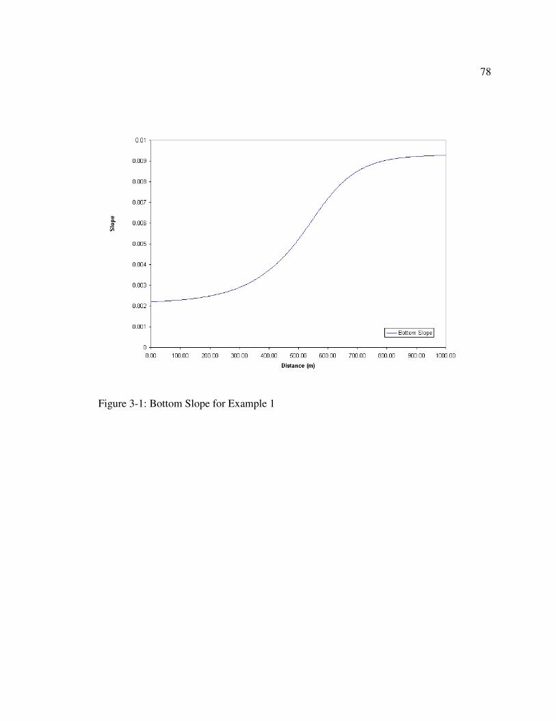
78
Figure 3-1: Bottom Slope for Example 1
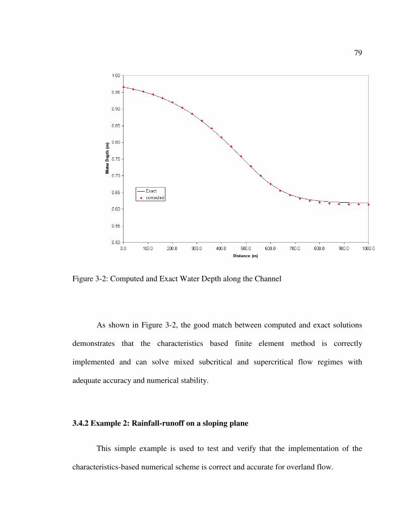
79
Figure 3-2: Computed and Exact Water Depth along the Channel
As shown in Figure 3-2, the good match between computed and exact solutions
demonstrates that the characteristics based finite element method is correctly
implemented and can solve mixed subcritical and supercritical flow regimes with
adequate accuracy and numerical stability.
3.4.2 Example 2: Rainfall-runoff on a sloping plane
This simple example is used to test and verify that the implementation of the
characteristics-based numerical scheme is correct and accurate for overland flow.
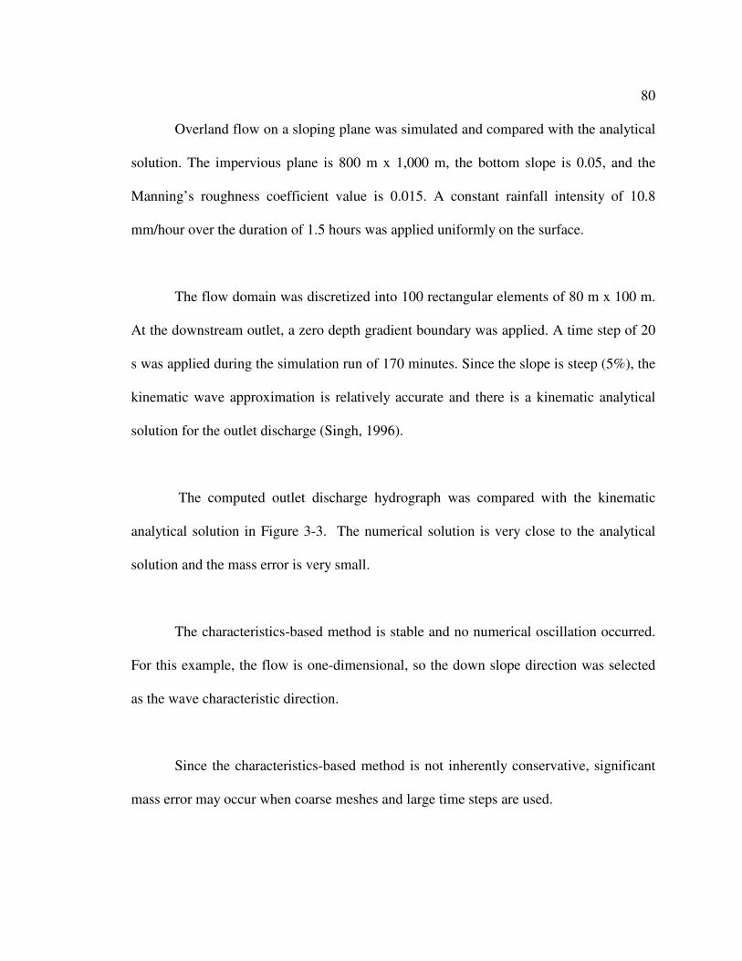
80
Overland flow on a sloping plane was simulated and compared with the analytical
solution. The impervious plane is 800 m x 1,000 m, the bottom slope is 0.05, and the
Manning’s roughness coefficient value is 0.015. A constant rainfall intensity of 10.8
mm/hour over the duration of 1.5 hours was applied uniformly on the surface.
The flow domain was discretized into 100 rectangular elements of 80 m x 100 m.
At the downstream outlet, a zero depth gradient boundary was applied. A time step of 20
s was applied during the simulation run of 170 minutes. Since the slope is steep (5%), the
kinematic wave approximation is relatively accurate and there is a kinematic analytical
solution for the outlet discharge (Singh, 1996).
The computed outlet discharge hydrograph was compared with the kinematic
analytical solution in Figure 3-3. The numerical solution is very close to the analytical
solution and the mass error is very small.
The characteristics-based method is stable and no numerical oscillation occurred.
For this example, the flow is one-dimensional, so the down slope direction was selected
as the wave characteristic direction.
Since the characteristics-based method is not inherently conservative, significant
mass error may occur when coarse meshes and large time steps are used.
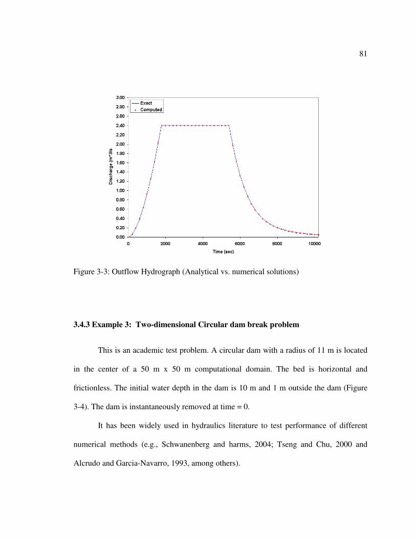
81
Figure 3-3: Outflow Hydrograph (Analytical vs. numerical solutions)
3.4.3 Example 3: Two-dimensional Circular dam break problem
This is an academic test problem. A circular dam with a radius of 11 m is located
in the center of a 50 m x 50 m computational domain. The bed is horizontal and
frictionless. The initial water depth in the dam is 10 m and 1 m outside the dam (Figure
3-4). The dam is instantaneously removed at time = 0.
It has been widely used in hydraulics literature to test performance of different
numerical methods (e.g., Schwanenberg and harms, 2004; Tseng and Chu, 2000 and
Alcrudo and Garcia-Navarro, 1993, among others).
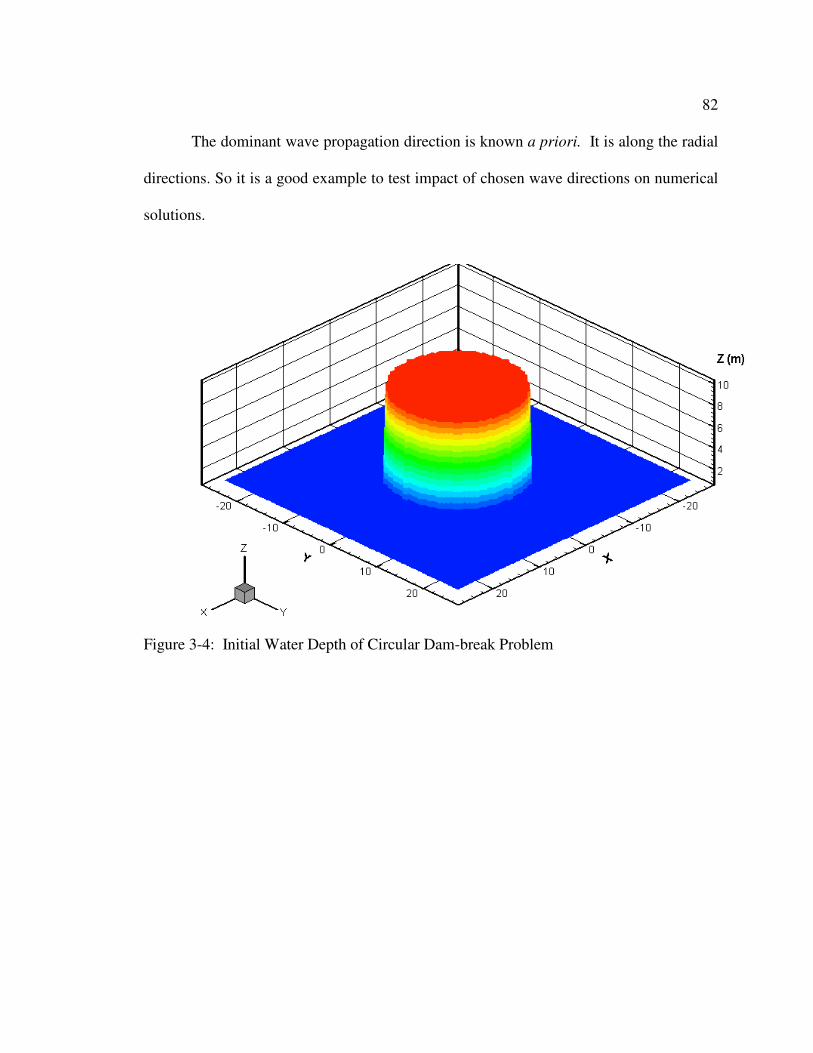
82
The dominant wave propagation direction is known a priori. It is along the radial
directions. So it is a good example to test impact of chosen wave directions on numerical
solutions.
Figure 3-4: Initial Water Depth of Circular Dam-break Problem
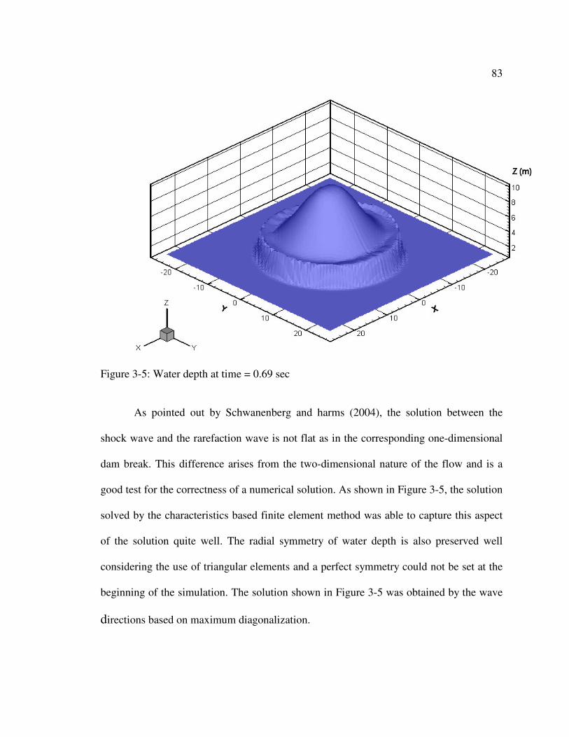
83
Figure 3-5: Water depth at time = 0.69 sec
As pointed out by Schwanenberg and harms (2004), the solution between the
shock wave and the rarefaction wave is not flat as in the corresponding one-dimensional
dam break. This difference arises from the two-dimensional nature of the flow and is a
good test for the correctness of a numerical solution. As shown in Figure 3-5, the solution
solved by the characteristics based finite element method was able to capture this aspect
of the solution quite well. The radial symmetry of water depth is also preserved well
considering the use of triangular elements and a perfect symmetry could not be set at the
beginning of the simulation. The solution shown in Figure 3-5 was obtained by the wave
directions based on maximum diagonalization.
84
The grid orientation effect of selected arbitrary wave directions was demonstrated in a
solution that used the x-direction (θ2 = 0) as the second characteristic direction. As can be
seen in Figure 3-6, a pre-specified characteristic direction cannot capture the two-
dimensional nature as well as by a dynamically computed wave direction, significant
spatial bias in the y-direction is revealed.
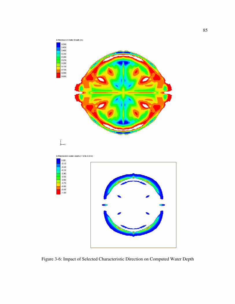
85
Figure 3-6: Impact of Selected Characteristic Direction on Computed Water Depth
86
3.4.4 Example 4: rainfall-runoff process over a three-plane cascade surface
This example is simulated to partially validate the appropriateness of the
governing equations for modeling the physical phenomena of overland flow by
comparison with experimental data. Furthermore, kinematic shock waves were generated
by the changes in bed slopes for the case of short rainfall duration (10 s) and it is a good
test of the capability of the numerical scheme in dealing with this.
Overland flow on a three-plane cascade surface was experimented by Iwagaki
(1955). A series of artificial rainfall was applied on a smooth aluminum laboratory flume
surface. The flume is 24 m in length and is divided into three planes with constant slopes
of 0.020, 0.015, and 0.010, respectively from upstream to downstream. The constant
rainfall intensities of 389, 230, and 288 cm/hour were applied to upper, middle and lower
plane, respectively, for the durations of 10 s, 20 s, and 30 s in three experiments.
The model simulations of the three-plane cascade example were made with a
uniform finite element mesh size of 0.25 m by 0.25 m. The whole plane surface
consisted of 768 elements and 873 nodes. A Manning’s roughness coefficient of 0.007
was used. No-flow boundary condition was applied except a critical flow condition was
used at the outlet. This is a one-dimensional flow problem, so the wave directions are
known a priori, and they are along the direction of the plane slopes.
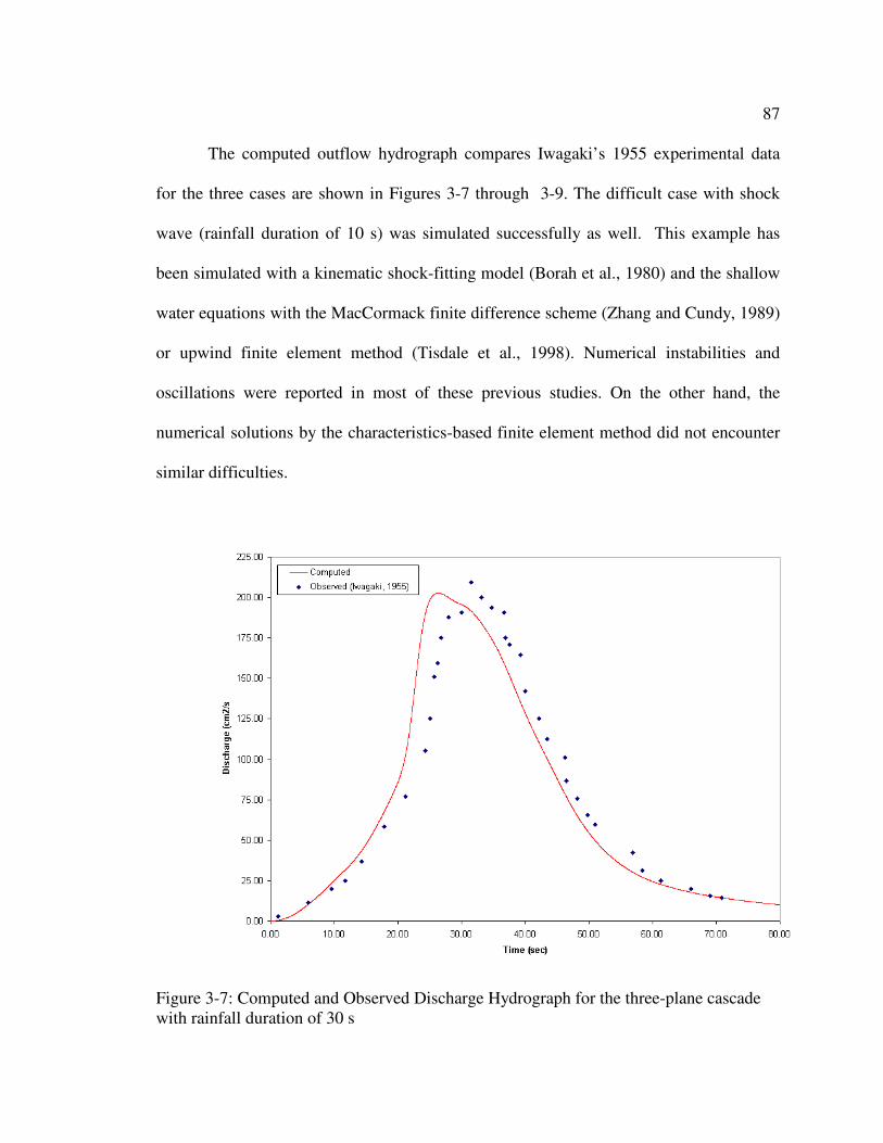
87
The computed outflow hydrograph compares Iwagaki’s 1955 experimental data
for the three cases are shown in Figures 3-7 through 3-9. The difficult case with shock
wave (rainfall duration of 10 s) was simulated successfully as well. This example has
been simulated with a kinematic shock-fitting model (Borah et al., 1980) and the shallow
water equations with the MacCormack finite difference scheme (Zhang and Cundy, 1989)
or upwind finite element method (Tisdale et al., 1998). Numerical instabilities and
oscillations were reported in most of these previous studies. On the other hand, the
numerical solutions by the characteristics-based finite element method did not encounter
similar difficulties.
Figure 3-7: Computed and Observed Discharge Hydrograph for the three-plane cascade
with rainfall duration of 30 s
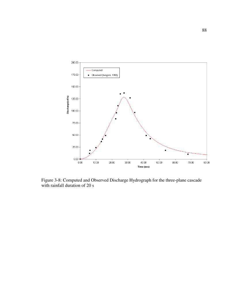
88
Figure 3-8: Computed and Observed Discharge Hydrograph for the three-plane cascade
with rainfall duration of 20 s
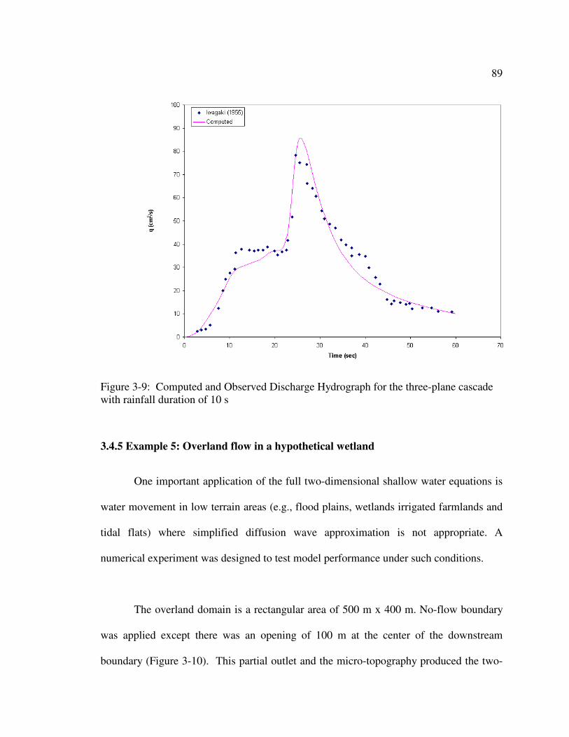
89
Figure 3-9: Computed and Observed Discharge Hydrograph for the three-plane cascade
with rainfall duration of 10 s
3.4.5 Example 5: Overland flow in a hypothetical wetland
One important application of the full two-dimensional shallow water equations is
water movement in low terrain areas (e.g., flood plains, wetlands irrigated farmlands and
tidal flats) where simplified diffusion wave approximation is not appropriate. A
numerical experiment was designed to test model performance under such conditions.
The overland domain is a rectangular area of 500 m x 400 m. No-flow boundary
was applied except there was an opening of 100 m at the center of the downstream
boundary (Figure 3-10). This partial outlet and the micro-topography produced the two-
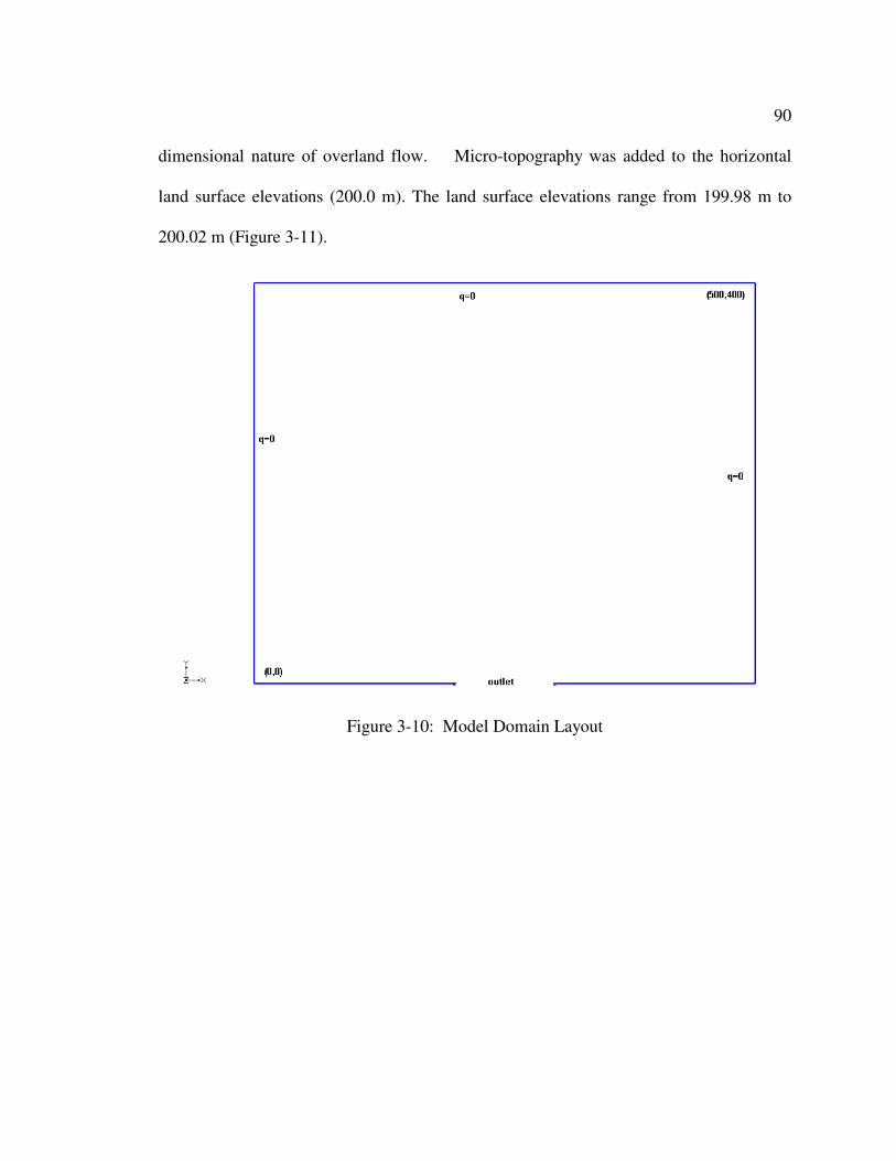
90
dimensional nature of overland flow. Micro-topography was added to the horizontal
land surface elevations (200.0 m). The land surface elevations range from 199.98 m to
200.02 m (Figure 3-11).
Figure 3-10: Model Domain Layout
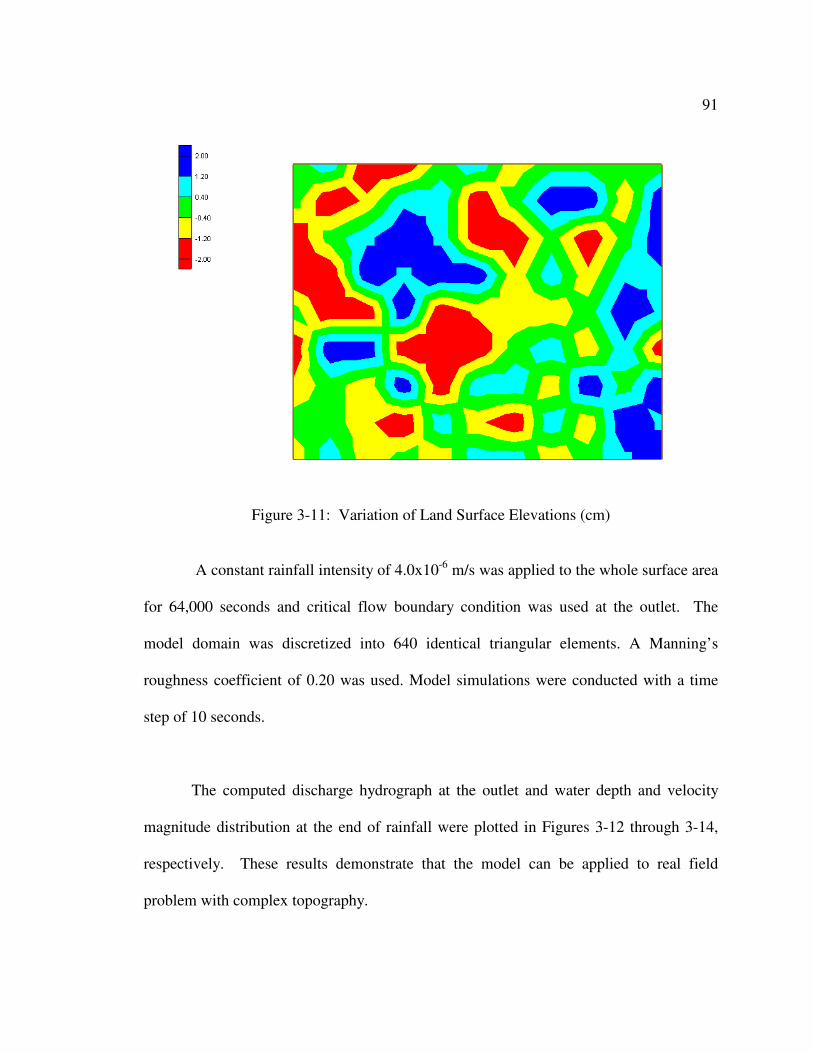
91
Figure 3-11: Variation of Land Surface Elevations (cm)
A constant rainfall intensity of 4.0x10⁻⁶
m/s was applied to the whole surface area
for 64,000 seconds and critical flow boundary condition was used at the outlet. The
model domain was discretized into 640 identical triangular elements. A Manning’s
roughness coefficient of 0.20 was used. Model simulations were conducted with a time
step of 10 seconds.
The computed discharge hydrograph at the outlet and water depth and velocity
magnitude distribution at the end of rainfall were plotted in Figures 3-12 through 3-14,
respectively. These results demonstrate that the model can be applied to real field
problem with complex topography.
92
The aforementioned simulation results were obtained by applying the diagonized
wave characteristic directions (the first approach in Section 3.3.2). Several other wave
characteristic directions were also tested for this example problem. These other wave
characteristic directions include: (1) the Froude line directions (the second approach); (2)
in the computed velocity direction; (3) fixed in the y-directions.
The computed water depth and velocity magnitude at the center of the domain
(x,y) = (250, 200) are compared in Figures 3-15 and 3-16. From the simulation results,
the use of the diagonized wave directions and computed velocity directions produce very
close water depth and velocity. On the other hand, the Froude line approach obtained
lowest computed water depth and highest velocity magnitude. The use of fixed y-
direction as wave characteristic directions results in computed water depth and velocity
between the ranges of results obtained with the other two approaches. This means that
selected wave directions have impact on simulation results.
Since the approaches using the diagonalization wave direction and computed
velocity direction yield very close simulations, we surmise that these simulations are the
correct solutions. On the other hand, we suspect that the simulations with the Froude line
approach or the fixed y-direction approach may have produced inaccurate solutions.
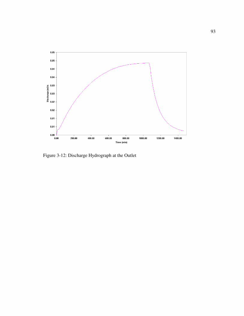
93
Figure 3-12: Discharge Hydrograph at the Outlet
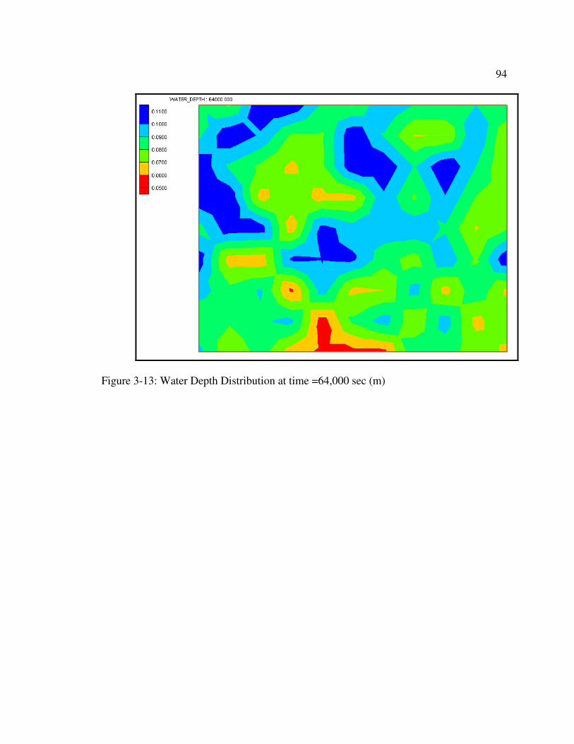
94
Figure 3-13: Water Depth Distribution at time =64,000 sec (m)
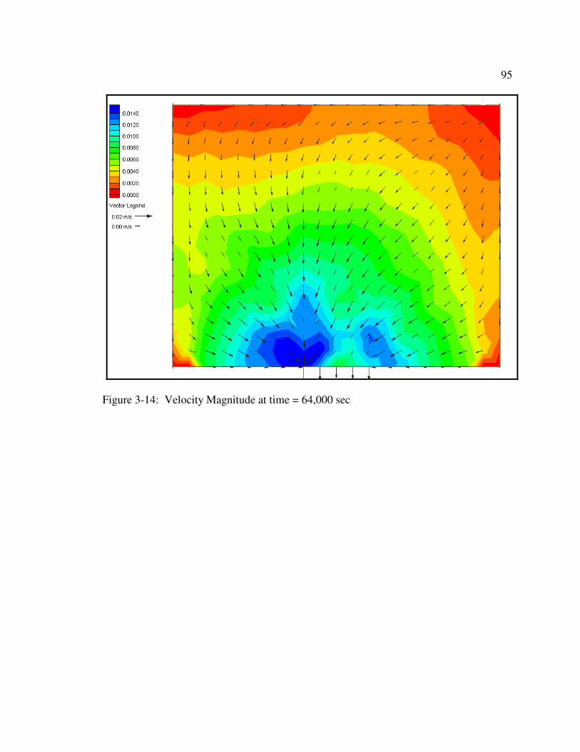
95
Figure 3-14: Velocity Magnitude at time = 64,000 sec
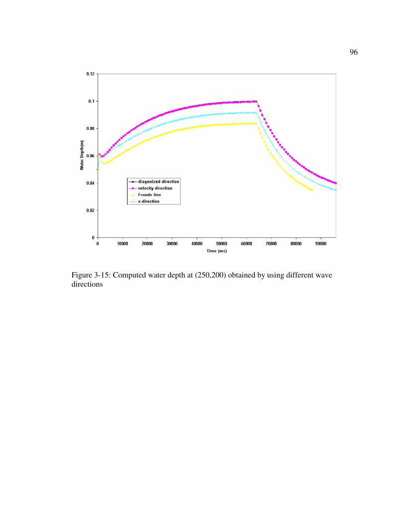
96
Figure 3-15: Computed water depth at (250,200) obtained by using different wave
directions
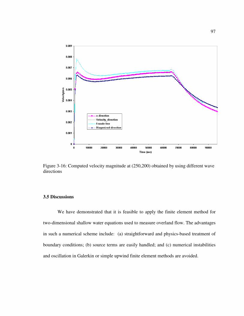
97
Figure 3-16: Computed velocity magnitude at (250,200) obtained by using different wave
directions
3.5 Discussions
We have demonstrated that it is feasible to apply the finite element method for
two-dimensional shallow water equations used to measure overland flow. The advantages
in such a numerical scheme include: (a) straightforward and physics-based treatment of
boundary conditions; (b) source terms are easily handled; and (c) numerical instabilities
and oscillation in Galerkin or simple upwind finite element methods are avoided.
98
By implementing the numerical schemes with linear finite elements, the accuracy
is first-order in space and time. Numerical diffusion is a major concern, however, the
maximum and minimum water depth were preserved satisfactory in the circular dam
break problem. A further work is to compare the performance of the current scheme with
the characteristic-based split (CBS) scheme (Zienkiewicz et al., 1999).
3.6 Summary and Conclusions
A characteristics based finite element method was applied to solve the two-
dimensional shallow water equations for overland flow. Implementation details,
especially the selection of characteristic wave directions, were discussed. In the selection
of wave characteristic directions, numerical simulations of the circular dam break and
overland flow in a hypothetical wetland, computed water depth, and velocity are affected.
Arbitrarily selected wave directions (e.g., x or y directions) result in less accurate results
in the circular dam break example. Further examination of this issue, with more test
examples having observed or exact solutions, is warranted.
It is concluded that this numerical method is very suitable for numerical solutions
of two-dimensional overland flow with thoughtful selection of wave characteristic
directions. One of this method’s advantages is that the treatment of the source term and
boundary conditions; they are straightforward and physically based. Further study is
needed to make it more stable for real watersheds with complex topography. Since the
99
Lagragian approach is not inherently mass conservative, careful checking of mass error is
a must for the model’s successful application.
Acknowledgements
This research is supported by the U.S. EPA - Science To Achieve Results (STAR)
Program under Grant # R-82795602 with the University of Central Florida.
References
Alcrudo, F. and Garcia-Navarro, P. (1993). “ A high-resolution Godunov-type scheme in
finite volumes for the 2D shallow water equations.”, International Journal of Numerical
Methods in Fluids, 16, 489-505.
Borah, DK; Prasad, SN; Alonso, CV. (1980). Kinematic Wave Routing Incorporating
Shock Fitting. Water Resources Research Vol 16, No 3, p 529-541, June 1980.
Brufau P., P. Garc_ıa-Navarro. (2003). Unsteady free surface flow simulation over
complex topography with a multidimensional upwind technique. Journal of
Computational Physics 186 (2003) 503–526.
100
Cheng H-P., Cheng J-R, Yeh GT. (1996). “ A particle tracking technique for the
Lagrangian-Eulerian finite element method in multi-dimensions.” International Journal
of Numerical Methods in Engineering. 39: 1115-1136.
Chow and Ben-Zvi. (1973). Hydrodynamic modeling of two-dimensional watershed
flow, Journal of Hydraulic Division ASCE, 99(HY1), P.2023--2024, 1973.
Fiedler F.R. and Ramirez J.A.. (2000). A numerical method for simulating discontinuous
shallow flow over an infiltrating surface. Int. J. Numer. Meth. Fluids 2000; 32: 219–240
Garcia-Navarro P., Hubbard M. and Priestley A. (1995). “ Genuinely multidimensional
upwinding for the 2D shallow water equations”, Journal of Computational Physics, Vol.
121, 79-93, 1995.
Guinot V. (2005). An approximate two-dimensional Riemann solver for hyperbolic
systems of conservation laws. Journal of Computational Physics, Volume 205, Issue 1,
p. 292-314.
Hirsch C., Lacon C. and Deconinck H. (1987). “Convection algorithms based on a
diagonalization procedure for the multidimensional Euler equations”, AIAA paper 87-
1163.
101
Iwagaki, Y. (1955). “ Fundamental studies on runoff analysis by characteristics.” Bull.
10, Disaster Prev. Res. Inst., Kyoto Univ., Kyoto, Japan, 1-25.
Katopodes N., T. Strelkoff. (1979) Two-dimensional shallow-water wave models, J. Eng.
Mech. Div., ASCE 105 (1979) 317–334.
Katopodes N., T. Strelkoff. (1978) Computing two-dimensional dam-break flood waves,
J. Hydraulics Div., ASCE Vol. 104, No. HY9 (1978) 1269–1288.
Katopodes, N.D. (1984). Dissipative Galerkin Scheme for Open-Channel Flow, Journal
of Hydraulic Engineering. Vol. 110, no. 4, pp. 450-466. Apr. 1984.
MacDonald I., Baines M., Nichols N. and Samuels P. (1997). “Analytical benchmark
solutions for open-channel flows”, Journal of Hydraulic Engineering, ASCE, Vol. 123,
No.11, November, 1997.
Paillère H., G. Degrez, H. Deconinck (1998). Multidimensional upwind schemes for the
shallow water equations, International Journal for Numerical Methods in Fluids,
Volume 26, Issue 8 , Pages 987 – 1000.
Singh, V.P. (1996). Kinematic wave modeling in water resources: surface water
hydrology, Wiley, New York.
102
Suk H-J. (2003). “ Development of 2-D and 3-D simulator for three-phase flow with
general initial and boundary conditions.” Ph.D. Dissertation, the Pennsylvania State
University, University Park, PA.
Schwanenberg D. and M. Harms M., (2004). Discontinuous Galerkin Finite-Element
Method for Transcritical Two-Dimensional Shallow Water Flows. J. Hydr. Engrg.
ASCE, Volume 130, Issue 5, pp. 412-421.
Tayfur G., Kavvas M., Govindaraju R. and Storm D. (1993). “Applicability of St. Venant
equations for two-dimensional overland flows over rough infiltrating surfaces”, Journal
of Hydraulic Engineering, ASCE, Vol. 119, No.1, January, 1993.
Tisdale T.S., Scarlatos, P.D., Hamrick, J.M. (1998). Streamline Upwind Finite-Element
Method for Overland Flow. Journal of Hydraulic Engineering, ASCE. Vol. 124, no. 4,
pp. 350-357. April 1998.
Tseng, M.H. and Chu, C. H. (2000). “Two-dimensional shallow water flows simulation
using TVD-MacCormack scheme.” Journal of Hydraulic Research, 38(2), 123-131.
Zhang W. and Cundy W. (1989). “Modeling of two-dimensional overland flow”, Water
Resources Research, Vol. 25, No. 9, Pages 2019 –2035, September, 1989.
103
Zhao, D. H., Shen, H. W., Tabios, G. Q., III, Lai, J. S., and Tan, W. Y. (1994). ‘‘Finite-
volume two-dimensional unsteady-flow model for river basins.’’ J. Hydr. Engrg.,
ASCE, 120(7), 863–883.
Zienkiewicz P. , Nithiarasu P., Codina R., Vazquez M. and Oritz P. (1999). The
characteristic-based split procedure: an efficient and accurate algorithm for fluid
problems. Int. J. Numer. Meth. Fluids 31: 359–392.
104
Chapter 4
A Comparative Study of coupling Approaches for Surface water and groundwater
interactions
Abstract
In the core of an integrated watershed model exists the coupling among surface
water and subsurface water flows. Recently, interest displayed in hydrology literature,
regarding fully coupled approach for surface water and groundwater interactions, has
increased. For example, the assumption of a gradient-type flux equation, based on
Darcy’s law (linkage term) and the numerical solution of all governing equations in a
single global matrix (VanderKwaak, 1999; Panday and Huyakorn, 2004 and Gunduz and
Aral, 2005) has been reported. However, this trend is unfounded. This paper argues that
this “fully coupled approach” is only a special case of all possible coupling combinations
and, if not applied with caution, the non-physics interface parameter becomes a
calibration tool. Generally, there are two cases of surface/subsurface coupling based on
the physical nature of the interface: continuous or discontinuous assumption; when a
sediment layer exists at the interface, the discontinuous assumption may be justified. As
for numerical schemes, there are three cases: time-lagged, iterative, and simultaneous
solutions. Since modelers often resort to the simplest, fastest schemes in practical
applications, it is desirable to quantify potential errors and the performance specific to
each coupling scheme. This paper evaluates these coupling schemes in a watershed
model, WASH123D. Numerical experiments are used to compare the performance of
105
each coupling approach for different types of surface water and groundwater interactions.
These experiments are done in terms of surface water and subsurface water solutions,
along with exchange flux (e.g. infiltration/seepage rate). It is concluded that different
coupling approaches are justified for flow problems of different spatial and temporal
scales and the physical setting of interfaces; however, the time-lagged approach should
be avoided since it is the least accurate approach.
4.1 Introduction
In the core of an integrated, physics-based watershed model is a study of coupling
among surface water and subsurface water flows. In this study, we focus on physics-
based coupling approaches that utilize partial differential equations both in surface water
flow (Saint Venant equations) and variably saturated subsurface flow models (Richards
equation). For simpler watershed models, the infiltration term is treated by an empirical
algebraic equation; accordingly, the surface water/groundwater interaction computation is
straightforward and independent of water flow solutions. Although the numerical solution
of the Richards equation is computationally intensive and difficult at watershed scales, it
is essential for a complete, physics-based representation of the subsurface flow.
The consideration of surface water/subsurface water interactions consists of two
parts: stream-aquifer interaction and overland-subsurface interaction. The stream-aquifer
interaction has been extensively studied by coupling saturated groundwater flow with
one-dimensional channel flow (for example, Pinder and Sauer, 1971; Swain and Wexler,
106
1996, and Hunt, 1990, among others). The role of unsaturated zone on stream-aquifer
interaction is rarely considered. The overland-subsurface interaction is usually studied in
the context of runoff generation at the watershed scales (for example, Freeze, 1972;
Smith and Woolhiser, 1971; Akan and Yen, 1981 and Abbott et al., 1986).
Recently, the physics-based coupling of surface and subsurface flows has been an
active research topic. Panday and Huyakorn (2004) discussed the utility of different
coupling schemes in a new watershed model and seemed to favor the conductance-type,
linkage term approach. Morita and Yen (2002) classified coupling approaches as fully
coupled (simultaneous solution), alternating iterative coupling and externally coupling
(decoupled). In their model, the concept of infiltrability was introduced. This term refers
to the variable boundary conditions in numerical solution of Richards equation; however,
a leakage term was used in the coupling process.
With the assumption of a linkage term at the interface, the full implicit coupling
approach has been tested in some recent models: InHM (VanderKwaak, 1999),
MODHMS (Panday and Huyakorn, 2004), and Gunduz and Aral (2005). Enhanced
numerical stability and accuracy were reported on some test examples as a result of
solving the coupled governing equations in a single global matrix. However, this
approach also has intrinsic limitations: an assumption has to be made that there exists a
discontinuous layer at the interface, and usually, identical time steps have to be used for
both surface water and subsurface flow.
107
Kollet and Maxwell (2005) pointed out the limitation of the linkage-term
approach, based on the interface conductance concept, and considered overland flow as
part of a subsurface flow boundary condition in their coupled model. The continuity of
pressure head at the interface was imposed. However, in their coupled model, the same
time step must be used for both overland and subsurface flow.
The time-lagged, decoupled approach is still very popular in some loosely
coupled models that consist of an existing surface water model and a subsurface flow
counterpart. Earlier studies make use of this approach to reduce computation effort.
Smith and Woolhiser (1971) coupled a one-dimensional Richards equation with one-
dimensional kinematic wave overland flow to simulate rainfall-runoff on a plane. Singh
and Bhallamudi (1998) developed a coupled overland flow model with one-dimensional
dynamic wave equations and two-dimensional Richards equation. The time-lagged,
decoupled approach was used for surface water/groundwater interaction. Langevin et al.
(2005) simulated the integrated surface water/groundwater interaction in coastal wetlands
in south Florida by coupling the two-dimensional hydrodynamic model (SWIFT2D) with
the SEWAT density-dependent groundwater model in a time-lagged, decoupled manner.
Although all the coupling approaches are conceptually simple, there seems to be no
consensus regarding the best approach in hydrology literature. The so-called ‘fully
coupled approach’ has a different definition and meaning for different people in current
108
hydrologic modeling research and practice; some refer to the inclusion of hydrological
processes while others refer to the coupling schemes.
It is also interesting to see how different coupling approaches can reach similar
results for the example problem of Smith and Woolhiser (1971). In their original paper, a
kinematic wave approximation was applied for overland flow and a time-lagged,
decoupled approach was used. Singh and Bhallamudi (1998) applied the full St. Venant
equations for overland flow with a decoupled scheme. Morita and Yen (2002) applied the
iterative coupling approach and VanderKwaak (1999) applied a linkage-term based
simultaneous coupling approach to the same problem. All models reported a close match
with the experiment data. A possible explanation is that the example is a typical
Hortonian runoff problem and subsurface flow contribution to surface runoff is not
important, so the surface/subsurface interaction is weak.
In this paper, the pros and cons of several combinations of coupling schemes,
including continuous or discontinuous interfaces, time-lagged, iterative, and simultaneous
solutions, will be discussed. The implementation of coupling schemes in a physics-
based, integrated watershed model (WASH123D), will be described; in addition, results
of numerical experiments will be compared in term of exchange flux (infiltration rate),
outlet discharge hydrograph, groundwater table, and soil moisture and computation time,
etc. The major motivation for such an analysis is that, in watershed and regional scale
practical applications, many simplifications and assumptions may have to be made on
surface water and groundwater interactions. The widely used weakly coupled, or
109
decoupled approaches were taken for the sole purpose of alleviating the computation
burden regardless if these approaches were adequate or not. In fact, examples shall
demonstrate that the decoupled approaches generally yield inadequate simulations. We
should fully understand the implication on the choice of coupling approaches on
simulation results.
4.2 Governing equations and Interface Conditions
Without losing generality, we will present the diffusion wave approximation to
the Saint Venant equations for surface water flows. And the three-dimensional Richards
equation is applied for subsurface flow. The interface conditions in connection to
source/sink terms and boundary conditions of the governing equations will be discussed.
4.2.1 Channel Network Flow
The governing equations of water flow in one-dimensional river/stream/canal can
be derived based on the conservation law of water mass and linear momentum. The
diffusion wave approximation is based on the continuity equation and a simplified form
of the momentum equation.
The continuity equation is:
OIERS SSSSSx
Q
t
A+−−+=
∂
∂+
∂
∂
(1)
110
where t is time [T]; x is the axis along the channel direction [L]; A is cross-sectional area
of the river/stream [L2]; Q is flow rate of the channel [L
3/T]; SS is the man-induced source
[L3/T/L]; SR is the source of direct rainfall [L
3/T/L]; SE is the sink due to
evapotranspiration [L3/T/L]; SI is the sink due to infiltration [L
3//T/L]; SO are the source
terms contributed from overland flow [L3/T/L].
In a diffusion wave approximation, the inertia terms in the momentum equation is
assumed negligible and the following velocity formula is applied:
x
H
x
H
x
Zn
RaV
o
∂
∂
∂
∂
∂
∂+
−=1
1
13/2
2
3/2
(2)
where n is Manning’s roughness [TL-1/3
], a is a unit-dependent factor (a = 1 for SI units
and a = 1.49 for U.S. Customary units) to make the Manning’s roughness unit-
independent, R is the hydraulic radius [L], Zo is channel bottom elevation above a datum
[L] and H = h + Zo is the water stage [L].
Using the definition Q = VA and substituting Eq. (2) into Eq. (1), we obtain
oIERS SSSSSx
HK
xt
HB +−−+=
∂
∂
∂
∂−
∂
∂ (3)
in which
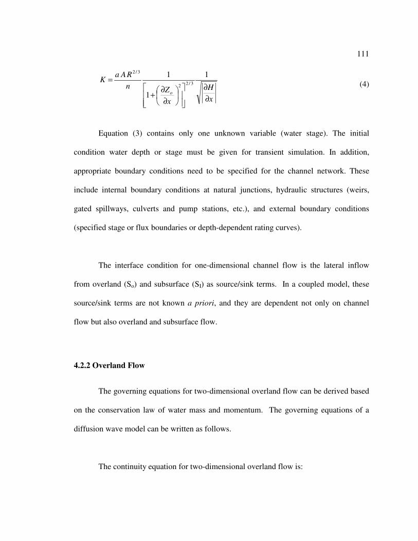
111
x
H
x
Zn
RAaK
o
∂
∂
∂
∂+
=1
1
13/2
2
3/2
(4)
Equation (3) contains only one unknown variable (water stage). The initial
condition water depth or stage must be given for transient simulation. In addition,
appropriate boundary conditions need to be specified for the channel network. These
include internal boundary conditions at natural junctions, hydraulic structures (weirs,
gated spillways, culverts and pump stations, etc.), and external boundary conditions
(specified stage or flux boundaries or depth-dependent rating curves).
The interface condition for one-dimensional channel flow is the lateral inflow
from overland (So) and subsurface (SI) as source/sink terms. In a coupled model, these
source/sink terms are not known a priori, and they are dependent not only on channel
flow but also overland and subsurface flow.
4.2.2 Overland Flow
The governing equations for two-dimensional overland flow can be derived based
on the conservation law of water mass and momentum. The governing equations of a
diffusion wave model can be written as follows.
The continuity equation for two-dimensional overland flow is:
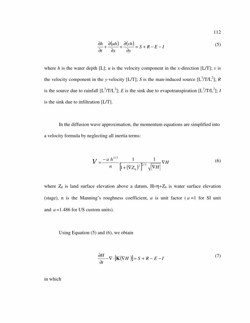
112
( ) ( )IERS
y
vh
x
uh
t
h−−+=
∂
∂+
∂
∂+
∂
∂
(5)
where h is the water depth [L]; u is the velocity component in the x-direction [L/T]; v is
the velocity component in the y-velocity [L/T]; S is the man-induced source [L3/T/L
2]; R
is the source due to rainfall [L3/T/L
2]; E is the sink due to evapotranspiration [L
3/T/L
2]; I
is the sink due to infiltration [L/T].
In the diffusion wave approximation, the momentum equations are simplified into
a velocity formula by neglecting all inertia terms:
( )[ ]H
HZn
haV ∇∇∇+
−=
1
1
13/22
0
3/2
(6)
where Ζ0 is land surface elevation above a datum, Η=η+Ζ0 is water surface elevation
(stage), n is the Manning’s roughness coefficient, a is unit factor ( a =1 for SI unit
and a =1.486 for US custom units).
Using Equation (5) and (6), we obtain
( )[ ] IERSHt
H−−+=∇⋅∇−
∂
∂K
(7)
in which
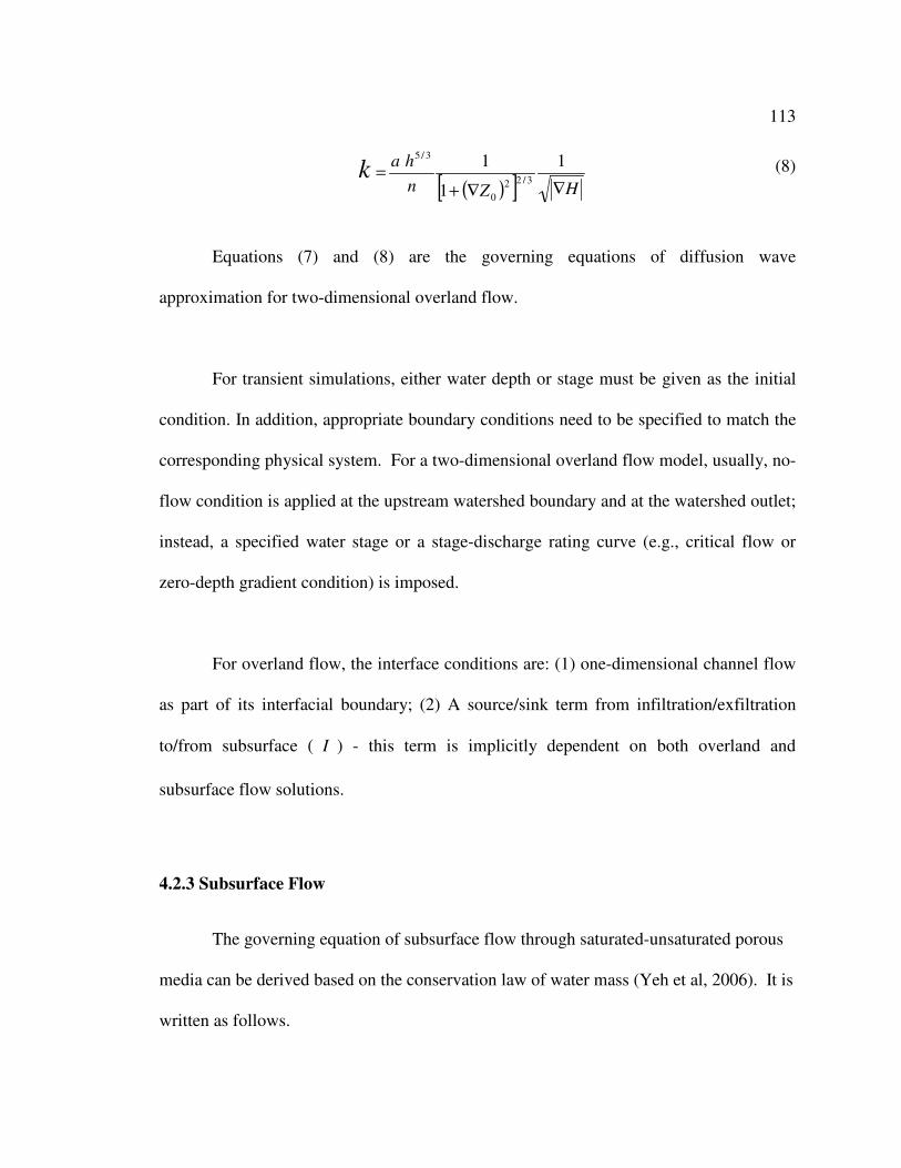
113
( )[ ] HZn
hak∇∇+
=1
1
13/22
0
3/5
(8)
Equations (7) and (8) are the governing equations of diffusion wave
approximation for two-dimensional overland flow.
For transient simulations, either water depth or stage must be given as the initial
condition. In addition, appropriate boundary conditions need to be specified to match the
corresponding physical system. For a two-dimensional overland flow model, usually, no-
flow condition is applied at the upstream watershed boundary and at the watershed outlet;
instead, a specified water stage or a stage-discharge rating curve (e.g., critical flow or
zero-depth gradient condition) is imposed.
For overland flow, the interface conditions are: (1) one-dimensional channel flow
as part of its interfacial boundary; (2) A source/sink term from infiltration/exfiltration
to/from subsurface ( I ) - this term is implicitly dependent on both overland and
subsurface flow solutions.
4.2.3 Subsurface Flow
The governing equation of subsurface flow through saturated-unsaturated porous
media can be derived based on the conservation law of water mass (Yeh et al, 2006). It is
written as follows.
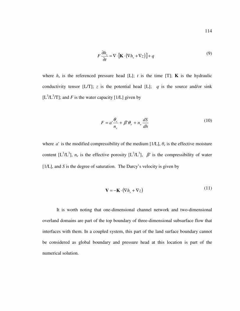
114
( )[ ] qzht
hF s
s +∇+∇⋅⋅∇=∂
∂K
(9)
where hs is the referenced pressure head [L]; t is the time [T]; K is the hydraulic
conductivity tensor [L/T]; z is the potential head [L]; q is the source and/or sink
[L3/L
3/T]; and F is the water capacity [1/L] given by
dh
dSn
naF ee
e
e ++= θβθ
'' (10)
where 'a is the modified compressibility of the medium [1/L], θe is the effective moisture
content [L3/L
3], ne is the effective porosity [L
3/L
3], 'β is the compressibility of water
[1/L], and S is the degree of saturation. The Darcy’s velocity is given by
( )zhs ∇+∇⋅−= KV (11)
It is worth noting that one-dimensional channel network and two-dimensional
overland domains are part of the top boundary of three-dimensional subsurface flow that
interfaces with them. In a coupled system, this part of the land surface boundary cannot
be considered as global boundary and pressure head at this location is part of the
numerical solution.
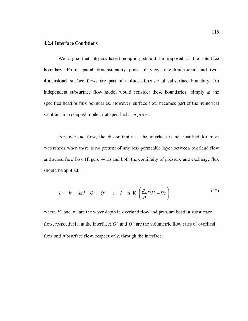
115
4.2.4 Interface Conditions
We argue that physics-based coupling should be imposed at the interface
boundary. From spatial dimensionality point of view, one-dimensional and two-
dimensional surface flows are part of a three-dimensional subsurface boundary. An
independent subsurface flow model would consider these boundaries simply as the
specified head or flux boundaries. However, surface flow becomes part of the numerical
solutions in a coupled model, not specified as a priori.
For overland flow, the discontinuity at the interface is not justified for most
watersheds when there is no present of any less permeable layer between overland flow
and subsurface flow (Figure 4-1a) and both the continuity of pressure and exchange flux
should be applied:
o s o s soh h and Q Q I h zρ
ρ
= = ⇒ = ⋅ ⋅ ∇ + ∇
n K
(12)
where oh and s
h are the water depth in overland flow and pressure head in subsurface
flow, respectively, at the interface; oQ and sQ are the volumetric flow rates of overland
flow and subsurface flow, respectively, through the interface.
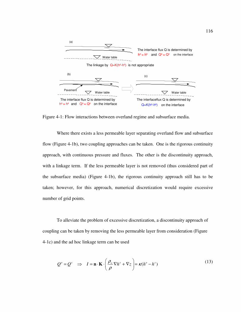
116
Water tableho = hs
The interface flux Q is determined by
Qo = Qsand on the interface
The linkage by Q=K(ho-hs) is not appropriate
(a)
Water tablePavement
Water table
The interface flux Q is determined by The interfaceflux Q is determined by
ho = hs Qo = Qsand on the interface Q=K(ho-hs) on the interface
(b)(c)
Figure 4-1: Flow interactions between overland regime and subsurface media.
Where there exists a less permeable layer separating overland flow and subsurface
flow (Figure 4-1b), two coupling approaches can be taken. One is the rigorous continuity
approach, with continuous pressure and fluxes. The other is the discontinuity approach,
with a linkage term. If the less permeable layer is not removed (thus considered part of
the subsurface media) (Figure 4-1b), the rigorous continuity approach still has to be
taken; however, for this approach, numerical discretization would require excessive
number of grid points.
To alleviate the problem of excessive discretization, a discontinuity approach of
coupling can be taken by removing the less permeable layer from consideration (Figure
4-1c) and the ad hoc linkage term can be used
( )o s s o soQ Q I h z h hρ
κρ
= ⇒ = ⋅ ⋅ ∇ + ∇ = −
n K
(13)
117
where κ is the conductance or the exchange coefficient which is equal to K/B (where K
and B are the hydraulic conductivity and thickness of the less permeable layer removed,
respectively). This approach is justifiable because κ is a physical parameter representing
the material property of the layer removed. This linkage term would be a good
approximation as long as the storage effect of the layer is negligible.
Similarly, the explicit linkage term can be applied to stream-aquifer interaction if
field evidence shows that a thin sediment layer exists at the streambed and the subsurface
flow domain will not include this sediment layer.
4.3 Numerical Schemes for Surface and Subsurface Flow Coupling
We will use a simple overland/subsurface flow-coupling example for the
illustration of rigorous, physics-based coupling approach. As shown in Figure 4-2, in this
simple example, there are 12 overland nodes and six elements in the two-dimensional
overland domain. The three-dimensional subsurface medium consists of 36 subsurface
nodes and 12 elements.
118
Figure 4-2: 2D overland and 3D subsurface finite element mesh for the coupling example
For decoupled flow simulations, there are 12 surface-flow equations for 12
overland unknowns (water depth) with 12 Qo(i), i =1, 2,.., 12 considered external
sources/sinks under diffusion wave approximation; and 36 subsurface-flow equations for
36 subsurface unknowns (pressure head) with 12 Qs(j), j = 1, 2,.., 12 considered external
boundary fluxes. However, for a coupled flow simulation, there are 12 additional
unknown overland source/sink terms Qo(i), i=1,12 and 12 unknown boundary fluxes for
subsurface, Qs(j), j=1,12. In total, there are 24 new unknowns that need 24 new equations
to close the mathematical formulation. These 24 equations are obtained from the
interface conditions.
119
Obviously, the continuity of interface fluxes: ( ) ( ), 1,2,..,12o sQ i Q i i= = provide
12 equations. The additional 12 equations are based on the physical condition of the
interface. For a continuous interface: ( ) ( ), 1,2,..,12s oh i h i i= = . Or if a discontinuous
interface exists: ( ) ( ) [ ( ) ( )], 1,2,..,12o s o sQ i Q i k h i h i i= = − = .
In summary, there are 72 equations for 72 unknowns (12 overland water depths,
ho, 36 subsurface pressure head, h
s, and 24 exchange fluxes which compose of 12
overland source/sink terms, Qo and 12 subsurface boundary fluxes Q
s).
Nominally, solving the coupled flow problem can be considered as the
simultaneous solution of these 72 algebraic equations. The time step size of both overland
and subsurface flow simulation has been assumed to be identical in the above discussion.
If k sub-time steps (e.g., seconds or minutes) are used in overland flow simulation within
a single subsurface flow time step (e.g., hours or days), the number of overland
unknowns (water depth) will be 12k and the channel sources/sinks for each sub-time step
are linearly interpolated in time from the sources/sink values at the beginning and end of
the subsurface time steps. This will provide additional interface equations for the
overland sub-time steps. Thus the total unknowns for the simultaneously coupled system
would be 12k of ho’s + 36 h
s’s + 12 Q
o’s + 12 Q
s’s.
(1) Time-lagged, decoupled approach
When a time lagged, decoupled approach is used; the infiltration rate is computed
by using surface water flow solutions from a previous time step. In this way, it can say
120
that the 24 interface equations become identity equations (the right-hand side terms are
known). The twelve overland algebraic equations and the 36 subsurface algebraic
equations can be solved sequentially. Under this case, sub-time steps for overland flow
can be easily implemented. However, the interface conditions are not strictly satisfied;
therefore, the accuracy of the coupled solution is not guaranteed. The time-lagged
approach can be applied to both discontinuous and continuous cases.
(2) Iterative implicit coupling approach
When the iterative coupling approach is adopted, the implicit nature is maintained
by iterative updating of the exchange flux and subsurface boundary:
For the case of discontinuous interface and a linkage-term coupling is used,
where k is the number of nonlinear coupling iteration for subsurface flow. Surface flow
solutions can take many sub-time steps within a single subsurface time step and it will be
solved within the subsurface nonlinear loop. Both continuous and discontinuous cases
can be tackled with iterative implicit approach.
(3) Fully implicit coupling approach
),()1,(),(01,
),()1,(
+∆+∆++∆+
∆++∆+
=
=kttSkttktt
kttoktts
hhfQ
hh
(14)
)()1,(),(01, +∆+∆++∆+ −=
kttSkttktt hhkQ (15)
121
The so-called fully implicit coupling approach is implemented in such a way that
the interface equations are literally solved with other equations simultaneously within a
single global matrix. The following conditions are imposed:
For continuous interface:
For discontinuous interface:
The simultaneous solution by a single global matrix is to make use of equations
(16) or (17) to eliminate the exchange flux terms by rearranging the exchange flux terms
in the algebraic equations.
In case of applying Equation (17), the flux terms in the subsurface equations and
the surface equations are replaced by the explicit linkage terms, the unknown water depth
of the surface water in the subsurface equations and the unknown pressure head of the
subsurface in the surface equations are solved together in a single global matrix.
For the continuous case (Equation (16)), by using the interface equations, the
surface equations can be added to the subsurface equations and the modified subsurface
( , ) ( , )
( , ) ( , )
s t t k o t t k
s t t k o t t k
h h
Q Q
+∆ +∆
+∆ +∆
=
=
(16)
)( ,,, ktt
s
ktt
c
ktthhcq
∆+∆+∆+ −= (17)
122
equations are solved for the final solution. Kollet and Maxwell (2005) implemented
overland flow as part of subsurface boundary and this can be considered as an example
for this case. Not specifically enforcing the continuity of both pressure and fluxes, the
substitution approach may yield mass errors due to numerical non-exactness. A more
rigorous approach is to consider Equation (16) along with the discretized overland
(surface water) flow equations (with unknowns ho and Q
o) and the disscretized subsurface
flow equations (with unknowns hs and Qs) as a system of simultaneous algebraic
equations [i.e., a single global matrix is consisting of discretized overland flow equations,
discretized subsurface flow equations, and Eq. (16)]. This rigorous approach numerically
ensure mass conservation across the interface.
Therefore, both cases of interface conditions can be tackled with this coupling
approach; the ad-hoc assumption of discontinuous interface to apply this coupling
approach seems unnecessary. However, this coupling approach is only convenient when
the time steps for both surface and subsurface water flows are identical. If sub-time steps
for surface flow are used, the implementation will involve more simultaneous unknowns,
which can be computationally very cumbersome and involved.
4.3.1 Coupling between overland flow and subsurface flow
For two-dimensional overland flow, if the finite element method is applied to
solve both subsurface and surface flow, each overland node will correspond to one
subsurface node. In this case, it is obvious that infiltration is acting as a source/sink term
123
for overland flow, while overland regime is part of subsurface internal interfacial
boundary. The detail of coupling between overland and subsurface flow has been
discussed.
4.3.2 Coupling between channel flow and subsurface flow
For stream-aquifer interaction, the most accurate representation would be that the
physical streambed geometry (true shape of cross-sections) is part of the subsurface top
boundary. Under this condition, several subsurface nodes are connected to a single cross-
section location of a stream reach (one node for stream flow). However, this is not
practical for most field problems. If such a fine-scale resolution were needed, then the
channel flow would be better simulated as two-dimensional overland flow. For a large-
scale problem, the grid size for the subsurface domain can be several orders greater than
that of channel flow; so, in a finite element model, there is only one subsurface node
connected to a cross-section of a stream reach. This is similar to the case of a finite
difference model, wherein a stream reach is connected to a grid cell of subsurface flow.
Therefore, there is already geometry mapping approximation for stream-aquifer
interaction. This means that the subsurface mesh/grid size at the stream location can have
a significant impact on the coupled simulation results. With this in mind, it is not
surprising that the use of a linkage term is a convenient way to compute the exchange
flux for stream-aquifer interactions and, in fact, current stream-aquifer interaction
modeling studies exclusively apply this approach.
124
In many occasions, the subsurface medium (in contact with the riverbed is
continuous or the thin sediment layer at the streambed) does not extend to most part of
the wetted perimeter. The leakage term is not justified. This continuous case is equivalent
to imposing a changing hydraulic head at the subsurface node in direct contact with
stream water. The exchange flux cannot be explicitly described as a function of stream
water depth and subsurface pressure head.
4.3.3 Coupling Procedure
The Picard method or the Newton-Raphson method is usually applied for the nonlinear
iteration in numerical solution of the Richards equation. A direct or iterative matrix
solver can be used to solve the linearized algebraic equations. The fully implicit coupled
approach is implemented in such a way to make use of the nonlinear iteration as a global
coupling iteration loop. If the computation time for surface flows is only a fraction of
three-dimensional subsurface flow, this is justified.
During a nonlinear iteration for subsurface flow, the numerical solution of surface
flow domains are obtained with sub-time steps and boundary conditions along with
computed infiltration rate (exchange flux) provided by updated subsurface flow solutions,
as illustrated in Figure 4-3 for coupled overland and subsurface flow and the coupling
procedure implemented in WASH123D is shown in Figure 4-4.
125
The calculation of infiltration rate is based on rainfall rate and water depth as
potential water supply (water available for infiltration); for the time-lagged approach,
overland water depth at the end of previous time step (hn) is applied during subsurface
flow computation to determine the possible infiltration rate. Then this computed
infiltration rate is used in two-dimensional overland flow computation of all two-
dimensional overland flow time steps within a three-dimensional time step. No feedback
mechanism is provided. For iterative coupling approach, the convergence of exchange
flux (infiltration rate) is checked with the updated pressure head and water depth. The
fully implicit coupling approach is such that the exchange-flux terms are eliminated from
the governing equations and the primary unknown variables - pressure head and water
depth, are literally solved in a single global matrix.
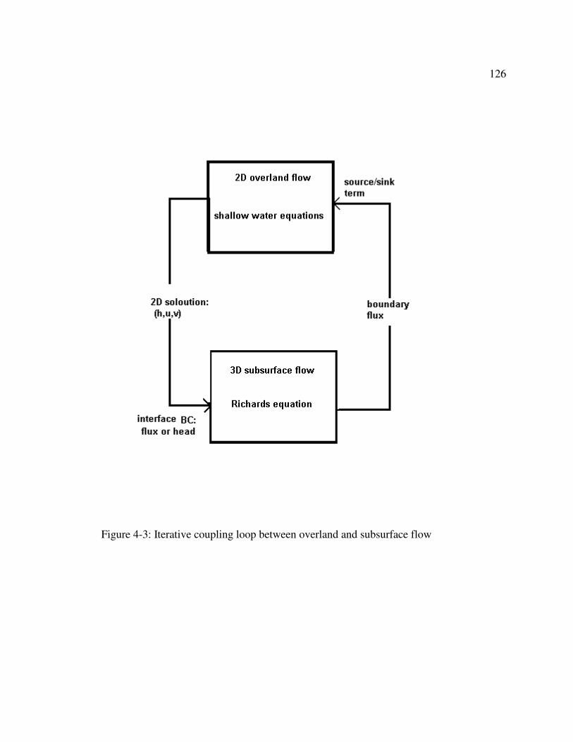
126
Figure 4-3: Iterative coupling loop between overland and subsurface flow
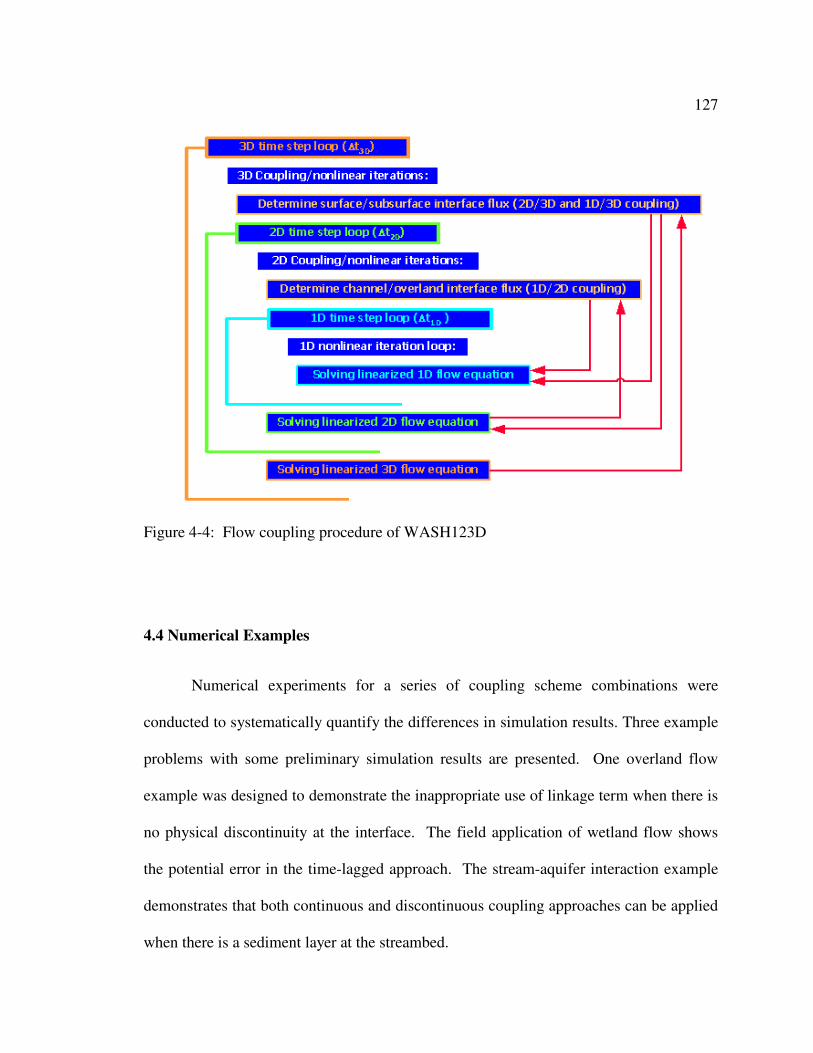
127
Figure 4-4: Flow coupling procedure of WASH123D
4.4 Numerical Examples
Numerical experiments for a series of coupling scheme combinations were
conducted to systematically quantify the differences in simulation results. Three example
problems with some preliminary simulation results are presented. One overland flow
example was designed to demonstrate the inappropriate use of linkage term when there is
no physical discontinuity at the interface. The field application of wetland flow shows
the potential error in the time-lagged approach. The stream-aquifer interaction example
demonstrates that both continuous and discontinuous coupling approaches can be applied
when there is a sediment layer at the streambed.
128
4.4.1 Coupled overland and subsurface flow: rainfall-runoff process
The first example is a simple case of rainfall-runoff process on a horizontal
surface of 500 m x 400 m. closed boundary was applied except a 100 m-outlet is located
at the center of a 500 m-side (critical flow) (Figure 4-5). The Manning’s n value is 0.02.
A rainfall intensity of 4.0E-5 m/s was applied for 600 minutes. The underlying porous
medium has a vertical saturated hydraulic conductivity of 5.5E-5 m/s and an effective
porosity of 0.41. There is no physical discontinuity of subsurface media at the interface.
Initially, the water table is 10 m below the land surface. No flow boundary was applied to
subsurface domain except the top boundary, which is the interface between overland and
subsurface domains. Constant time steps of 20 s and 180 s were applied for two-
dimensional overland flow and three-dimensional subsurface flow, respectively. The 900-
minute simulations were performed with the continuous coupling approach and the
linkage-term coupling approach and the outflow discharge hydrographs were compared
(Figure 4-6).
The computed outflow discharge hydrograph represents the integrated results of
rainfall, surface runoff and infiltration processes. It can be seen from Figure 4-6 that the
linkage-term and continuous coupling approaches resulted in different rising part of the
flow hydrograph. After the subsurface domain is fully saturated and the runoff became
steady, the simulation results are essentially the same. Since physically, there is no
discontinuous interface, the conductance values (k) were tested for three cases (k = 5.5E-
6, 5.5E-4 and 3.0E-3). A small k value constrains exchange fluxes; therefore, land surface
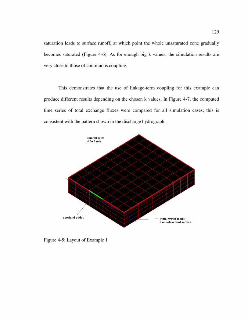
129
saturation leads to surface runoff, at which point the whole unsaturated zone gradually
becomes saturated (Figure 4-6). As for enough big k values, the simulation results are
very close to those of continuous coupling.
This demonstrates that the use of linkage-term coupling for this example can
produce different results depending on the chosen k values. In Figure 4-7, the computed
time series of total exchange fluxes were compared for all simulation cases; this is
consistent with the pattern shown in the discharge hydrograph.
Figure 4-5: Layout of Example 1
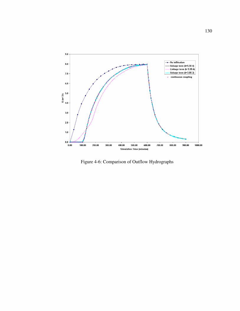
130
Figure 4-6: Comparison of Outflow Hydrographs
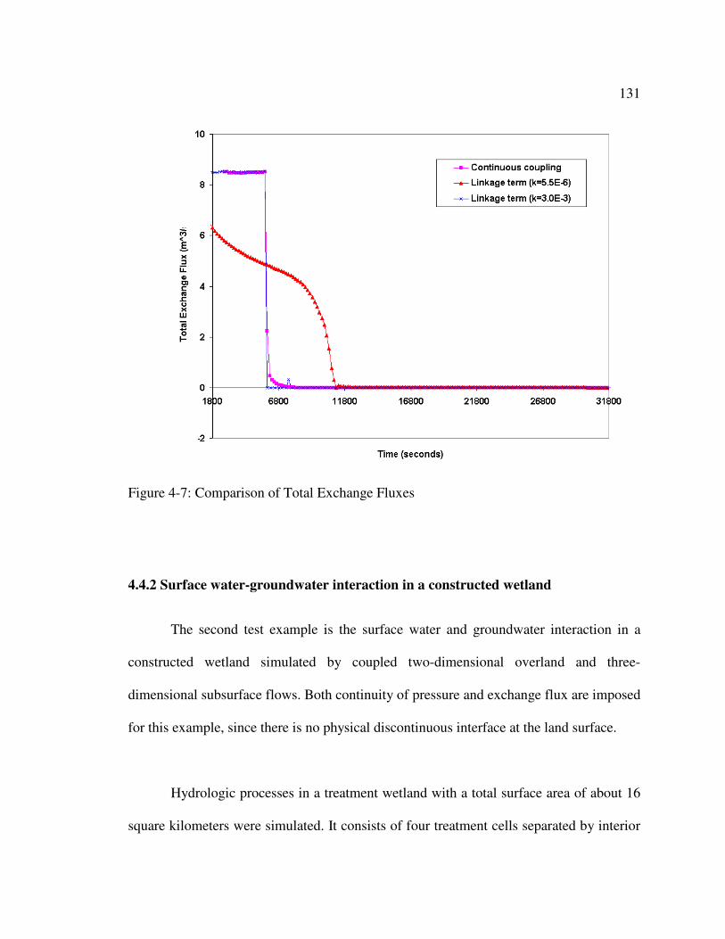
131
Figure 4-7: Comparison of Total Exchange Fluxes
4.4.2 Surface water-groundwater interaction in a constructed wetland
The second test example is the surface water and groundwater interaction in a
constructed wetland simulated by coupled two-dimensional overland and three-
dimensional subsurface flows. Both continuity of pressure and exchange flux are imposed
for this example, since there is no physical discontinuous interface at the land surface.
Hydrologic processes in a treatment wetland with a total surface area of about 16
square kilometers were simulated. It consists of four treatment cells separated by interior
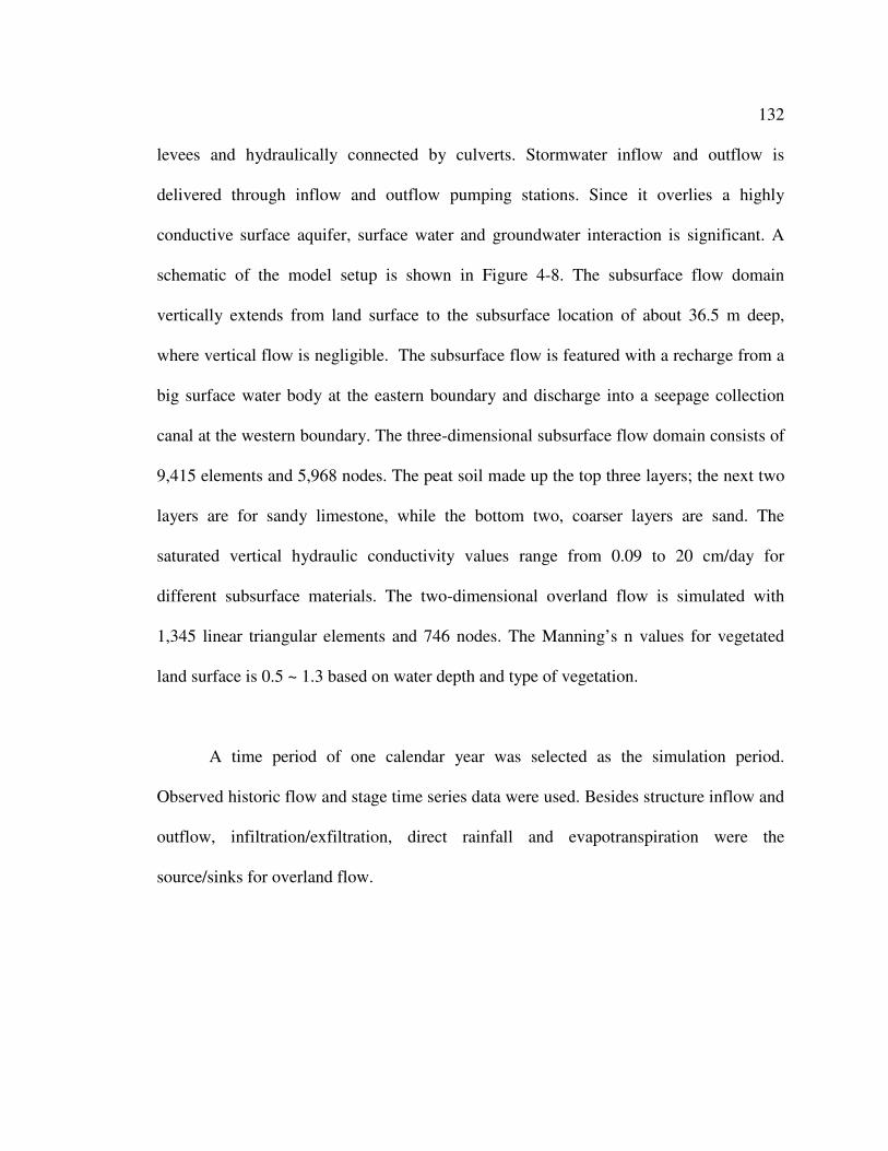
132
levees and hydraulically connected by culverts. Stormwater inflow and outflow is
delivered through inflow and outflow pumping stations. Since it overlies a highly
conductive surface aquifer, surface water and groundwater interaction is significant. A
schematic of the model setup is shown in Figure 4-8. The subsurface flow domain
vertically extends from land surface to the subsurface location of about 36.5 m deep,
where vertical flow is negligible. The subsurface flow is featured with a recharge from a
big surface water body at the eastern boundary and discharge into a seepage collection
canal at the western boundary. The three-dimensional subsurface flow domain consists of
9,415 elements and 5,968 nodes. The peat soil made up the top three layers; the next two
layers are for sandy limestone, while the bottom two, coarser layers are sand. The
saturated vertical hydraulic conductivity values range from 0.09 to 20 cm/day for
different subsurface materials. The two-dimensional overland flow is simulated with
1,345 linear triangular elements and 746 nodes. The Manning’s n values for vegetated
land surface is 0.5 ~ 1.3 based on water depth and type of vegetation.
A time period of one calendar year was selected as the simulation period.
Observed historic flow and stage time series data were used. Besides structure inflow and
outflow, infiltration/exfiltration, direct rainfall and evapotranspiration were the
source/sinks for overland flow.
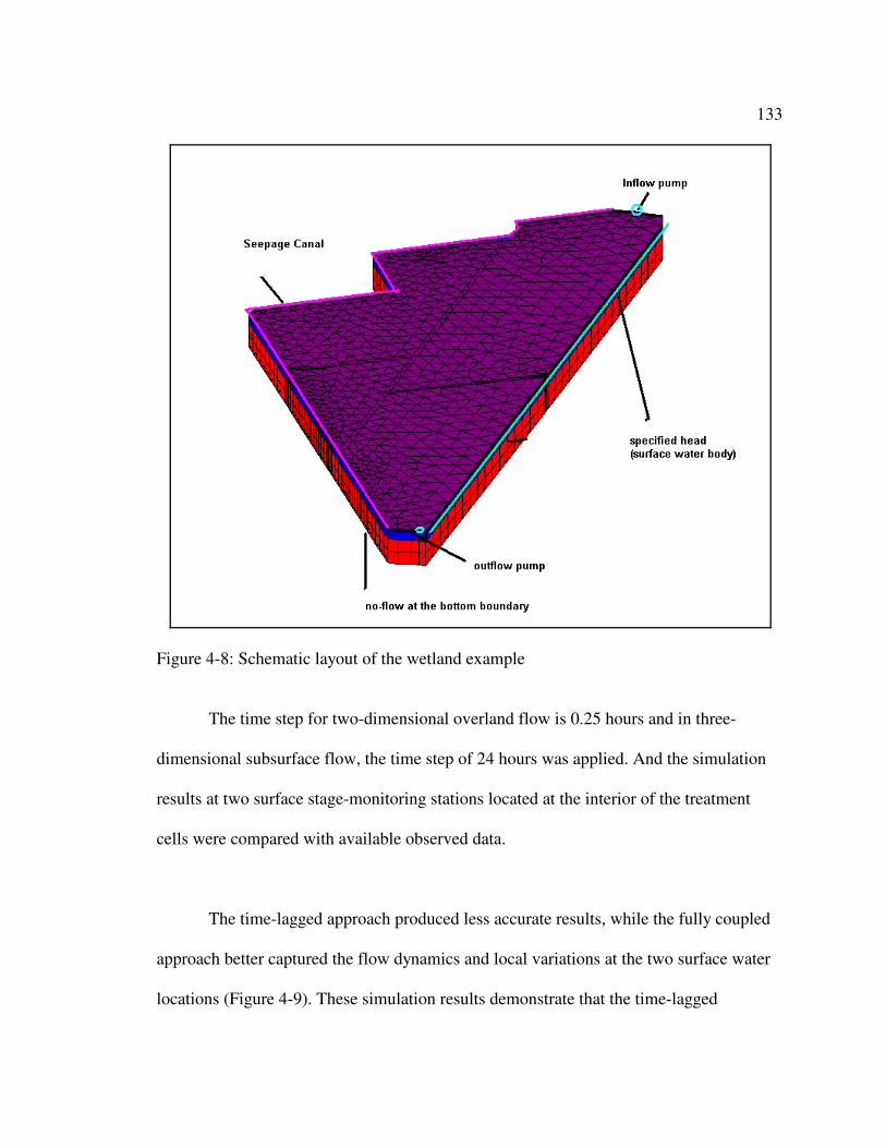
133
Figure 4-8: Schematic layout of the wetland example
The time step for two-dimensional overland flow is 0.25 hours and in three-
dimensional subsurface flow, the time step of 24 hours was applied. And the simulation
results at two surface stage-monitoring stations located at the interior of the treatment
cells were compared with available observed data.
The time-lagged approach produced less accurate results, while the fully coupled
approach better captured the flow dynamics and local variations at the two surface water
locations (Figure 4-9). These simulation results demonstrate that the time-lagged
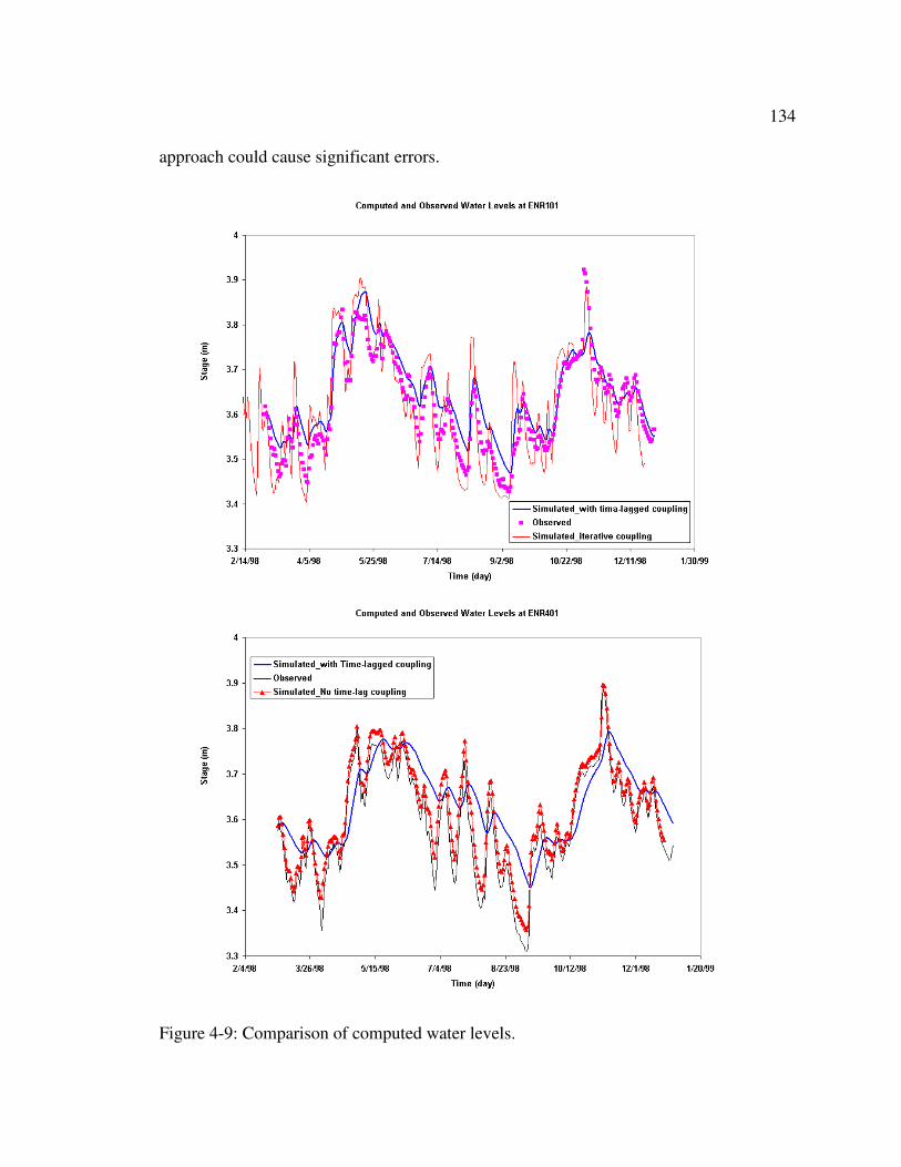
134
approach could cause significant errors.
Figure 4-9: Comparison of computed water levels.
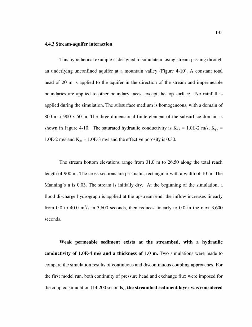
135
4.4.3 Stream-aquifer interaction
This hypothetical example is designed to simulate a losing stream passing through
an underlying unconfined aquifer at a mountain valley (Figure 4-10). A constant total
head of 20 m is applied to the aquifer in the direction of the stream and impermeable
boundaries are applied to other boundary faces, except the top surface. No rainfall is
applied during the simulation. The subsurface medium is homogeneous, with a domain of
800 m x 900 x 50 m. The three-dimensional finite element of the subsurface domain is
shown in Figure 4-10. The saturated hydraulic conductivity is Kxx = 1.0E-2 m/s, Kyy =
1.0E-2 m/s and Kzz = 1.0E-3 m/s and the effective porosity is 0.30.
The stream bottom elevations range from 31.0 m to 26.50 along the total reach
length of 900 m. The cross-sections are prismatic, rectangular with a width of 10 m. The
Manning’s n is 0.03. The stream is initially dry. At the beginning of the simulation, a
flood discharge hydrograph is applied at the upstream end: the inflow increases linearly
from 0.0 to 40.0 m3/s in 3,600 seconds, then reduces linearly to 0.0 in the next 3,600
seconds.
Weak permeable sediment exists at the streambed, with a hydraulic
conductivity of 1.0E-4 m/s and a thickness of 1.0 m. Two simulations were made to
compare the simulation results of continuous and discontinuous coupling approaches. For
the first model run, both continuity of pressure head and exchange flux were imposed for
the coupled simulation (14,200 seconds), the streambed sediment layer was considered
136
as part of subsurface media. The coupled simulation applies different time steps of 100
seconds for subsurface flow and 10 seconds for channel flow. For the second simulation,
the streambed sediment layer was removed from subsurface domain, and the leakage
term was applied to compute exchange rate. Figures 4-11 and 4-12 show impact of
stream seepage on subsurface pressure head distribution and only saturated zones are
plotted for the simulation results with continuous interface assumption. Figure 4-12 is the
computed river discharge hydrograph at two different locations under coupled flow and
solved with different coupling approaches. As expected, the flood peak water levels are
attenuated by stream-aquifer interaction.
For this specific example, similar results were obtained with both coupling
approaches; however, the differences are visible since the sediment layer was represented
by only one subsurface element in the vertical direction when both continuity of state
variables and exchange fluxes are imposed. Another reason for the difference is that the
storage effect of the sediment layer is not considered in the discontinuity approach of a
linkage term. As a result, infiltration will start earlier and the magnitude of infiltration
rate will increase for the case of discontinuity approach (Figure 4-14). This would delay
and decrease the magnitude of the surface runoff, i.e., the river discharge will be delayed
and its magnitude will decrease. The differences also increase as the flood wave moves
to the downstream boundary. Mesh refinement for the sediment layer will improve the
accuracy of computed exchange fluxes. When the hydraulic conductivity of the
streambed sediment is of several orders of magnitude smaller than that of the underlying
137
subsurface media, difficulty in obtaining convergent solutions, coupled with longer
computer run-times, are the major disadvantages of using the continuous approach.
0
10
20
30
40
50
Z
200
400
600
800
X
0
200
400
600
800
Y
X Y
Z
Figure 4-10: Three-dimensional finite element mesh
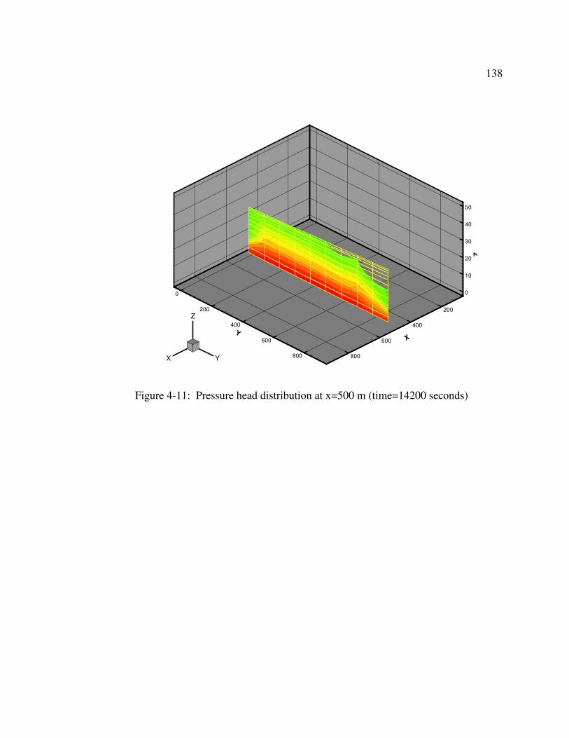
138
0
10
20
30
40
50
Z
200
400
600
800
X
0
200
400
600
800
Y
X Y
Z
Figure 4-11: Pressure head distribution at x=500 m (time=14200 seconds)
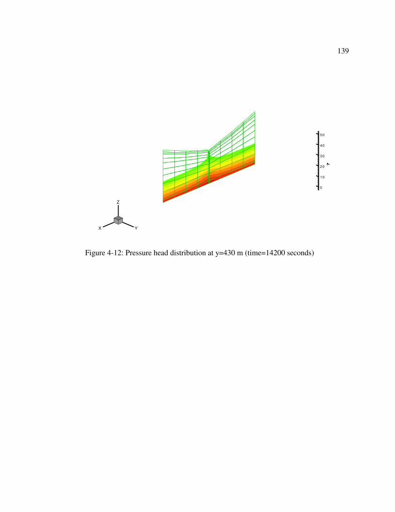
139
0
10
20
30
40
50
Z
X Y
Z
Figure 4-12: Pressure head distribution at y=430 m (time=14200 seconds)
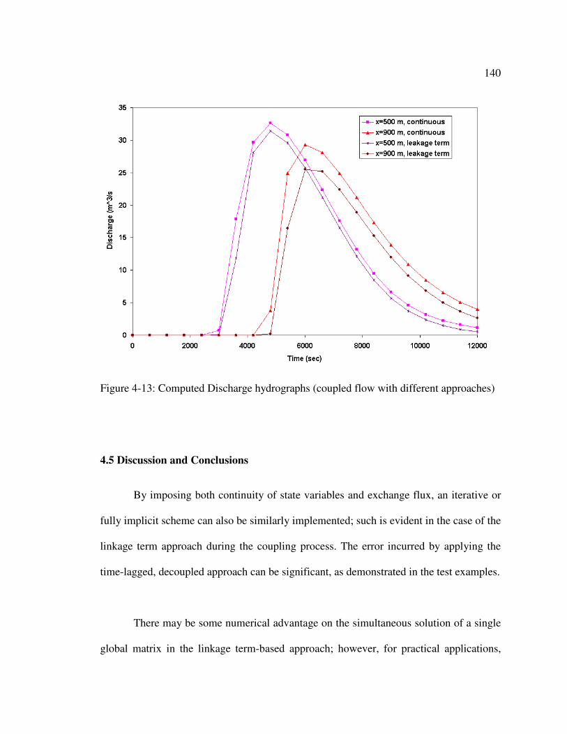
140
4.5 Discussion and Conclusions
By imposing both continuity of state variables and exchange flux, an iterative or
fully implicit scheme can also be similarly implemented; such is evident in the case of the
linkage term approach during the coupling process. The error incurred by applying the
time-lagged, decoupled approach can be significant, as demonstrated in the test examples.
There may be some numerical advantage on the simultaneous solution of a single
global matrix in the linkage term-based approach; however, for practical applications,
Figure 4-13: Computed Discharge hydrographs (coupled flow with different approaches)
141
identical time steps have to be used for both surface and subsurface flow; this paper has
also demonstrated this simultaneous coupling approach can also be implemented with
continuous interface conditions.
When discontinuous interface coupling is used, evidence and parameters from
field observation should be able to support such an assumption. For real-world
applications, many options must be provided; specifically, those that can be justified for
coupled flow problems of different spatial and temporal scales and the physical setting of
the interface.
Acknowledgements
This research is supported by the U.S. EPA – Science To Achieve Results (STAR)
Program under Grant # R-82795602 with the University of Central Florida.
References
Abbott, M.B., J.C. Bathurst, J.A. Cunge, P.E. O’Connell, and J. Rasmussen, (1986), An
introduction to the European Hydrological System- Systeme Hydrologique Europeen,
“SHE”, 2: Structure of a physically-based, distributed modeling system, Journal of
Hydrology, 87, 61-77, 1986.
A.O. Akan and B.C. Yen, (1981), Mathematical model of shallow water flow over porous
media. J. Hydraul. Div. 107 HY4 (1981), pp. 479–494.
142
R.A. Freeze, Role of subsurface flow in generating surface runoff. (1972), 1. Base flow
contributions to channel flow. Water Resour. Res. 8 (1972), pp. 609–623.
Gunduz O. and Aral M.M., (2005), River networks and groundwater flow: a
simultaneous solution of a coupled system. Journal of Hydrology. 2005; 301: 216-34.
Hunt B., (1990), An approximation for the bank storage effect, Water Resources
Research, Vol.26 No.11, Pages 2769-2775.
Kollet S.J. and Maxwell R.M.. (2005), Integrated surface-groundwater flow modeling: A
free-surface overland flow boundary condition in parallel groundwater flow model.
Advances in Water Resources, Volume 29, Issue 7, July 2006, Pages 945-958.
Langevin C., Swain E., and Wolfert M., (2005), Simulation of integrated surface-
water/ground-water flow and salinity for a coastal wetland and adjacent estuary,
Journal of Hydrology, Volume 314, Issues 1-4, 25 November 2005, Pages 212-234.
Morita M, Yen BC. , (2000), Numerical methods for conjunctive two-dimensional
surface and three-dimensional sub-surface flows. International Journal for Numerical
Methods in Fluids 32: 921–957.
143
Morita M, Yen BC. (2002), Modeling of conjunctive two-dimensional surface–three-
dimensional subsurface flows. Journal of Hydraulic Engineering, ASCE 128: 184–200.
Panday S. and Huyakorn P.S., (2004), A fully coupled physically-based spatially-
distributed model for evaluating surface/subsurface flow, Advances in Water
Resources, 27 (2004) 361–382
G.F. Pinder and S.P. Sauer, (1971), Numerical simulation of flow wave modification due
to back storage effects. Water Resour. Res. 7 1 (1971), pp. 63–70.
V. Singh and S.M. Bhallamudi, (1998), Conjunctive surface–subsurface modeling of
overland flow. Adv. Water Resour. 21 (1998), pp. 567–579.
Smith, R. E., and Woolhiser, D. A. (1971). ‘‘Overland flow on an infiltration surface,’’
Water Resour. Res., 7(4), 899–913.
Swain ED, Wexler EJ, (1996), A coupled surface-water and groundwater flow model for
simulation of stream–aquifer interaction. US geological survey techniques of water-
resources investigations, Book 6; 1996. 125 p [chapter A6].
144
VanderKwaak JE., (1999), Numerical simulation of flow and chemical transport in
integrated surface–subsurface hydrologic systems, Doctorate Thesis, Department of
Earth Sciences, University of Waterloo, Ontario, Canada.
Yeh, G.T., G. B. Huang, H. P. Cheng, F. Zhang, H. C. Lin, E. Edris, and D. Richards.
(2006). A first principle, physics-based watershed model: WASH123D, in Watershed
Models. Eds. By Singh VP and Frevert D.K., CRC Press, Boca Raton, FL.
145
Chapter 5
Integrated Modeling of Groundwater and Surface Water interactions in a
constructed wetland
Abstract
As a man-made pilot wetland in south Florida, USA, the Everglades Nutrient
Removal (ENR) project was modeled with a physics-based integrated approach using
WASH123D. Stormwater is routed into the treatment wetland for phosphorus removal by
plant and sediment uptake. It overlies a highly permeable surficial groundwater aquifer.
Strong surface water and groundwater interactions are a key component of the hydrologic
processes. The site has extensive field measurement and monitoring tools that provide
point scale and distributed data on surface water levels, groundwater levels, and the
physical range of hydraulic parameters and hydrologic fluxes. Previous hydrologic and
hydrodynamic modeling studies have treated seepage losses empirically by some simple
regression equations and, only surface water flows are modeled in detail. Several years
of operational data are available and were used in model calibration and validation. The
validity of a diffusion wave approximation for 2-D overland flow (in the region with very
flat topography) was also tested. The uniqueness of this modeling study includes (1) the
point scale and distributed comparison of model results with observed data; for example,
the spatial distribution of measured vertical flux in the wetland is available; (2) model
parameters are based on available field test data; (3) water flows in the study area consist
of 2-D overland flow, hydraulic structures/levees, 3-D subsurface flow and 1-D canal
146
flow and their interactions. This study demonstrates the need and the utility of a physics-
based modeling approach for strong surface water and groundwater interactions.
5.1 Introduction
Man-made treatment wetlands have been extensively used for wastewater
treatment or stormwater nutrient removal in the USA. Typically, these surface water
impoundments are built for flow-through treatment of stormwater by plant and sediment
uptakes of both nutrients and pollutants. In South Florida, the Everglades restoration
effort has led to the design and construction of a series of constructed wetlands, called
Stormwater Treatment Areas (STAs), to reduce phosphorus levels in stormwater runoff
before they can enter the Everglades protection areas. These constructed wetlands were
located on former natural wetlands or farmland. The Everglades Nutrient Removal (ENR)
project is a pilot constructed wetland for STAs (SFWMD, 2000).
In south Florida, the regional hydrogeology was characterized by the surficial
aquifer (Fish, 1988). Wetlands in the region have strong hydraulic connections with the
underlying, highly conductive surficial aquifer. Harvey et al. (2002) studied the surface
and groundwater interactions in the ENR and surrounding wetlands with field
investigations.
Guardo studied water budgeting in the ENR with a simple water mass balance
approach (Guardo, 1999). Regression models were used to estimate groundwater
147
seepages in ENR and the whole ENR was treated as a point for water budget. Guardo
and Tomasello (1995) simulated overland flow in ENR using a steady hydrodynamic
model. Until recently, the hydraulic models applied to the design and management of
constructed wetlands are quite limited in scope and detail. Most models are two-
dimensional, for steady-state flow. They are good for both design purposes or as a
screening tool, but lack important details [incorporating hydraulic structures, calibrated
model parameters and surface/groundwater interaction]. More detailed two-dimensional
hydraulic models, used in the existing treatment of wetlands, are being built for
management and operation needs. They are calibrated and validated with historic time
series data, considering only the two-dimensional surface flow.
Some popular hydrodynamic computer codes currently used for modeling wetland
hydraulics are originally developed for coastal hydrodynamic modeling. Some limitations
need to be addressed before they can be applied for wetland simulation. For instance, the
incorporation of hydraulic structures, explicit representation of rainfall, and evaporation
and treatment of wetting and drying are very important in a wetland hydrologic model.
Swain et al. (2004) has described their experience in adapting and modifying the
USGS SWIFT2D, originally developed for coastal tidal flow, to simulate the southern
Everglades wetland hydrology. A watershed model code, such as WASH123D (Yeh et
al., 2006) does not have these limitations. This WASH123D application is an example of
coupled surface/subsurface water flows in a constructed wetland for stormwater treatment
in south Florida. Current two-dimensional hydraulic models cannot handle seepage loss
148
properly; therefore, an integrated surface/groundwater model is needed to study the
dynamic interaction of surface flow within the treatment area and seepage loss through
bottom and perimeter levees. A one-dimensional canal flow is also needed to simulate
inflow/outflow and seepage collection. The impact of neglecting seepage loss is a likely
distorted hydraulic model.
Wetland hydrological modeling studies have been increasingly reported in the
hydrology literature. Feng and Molz (Feng and Molz, 1997) developed a surface water
flow model for wetlands with the diffusion wave approximation of the 2-D shallow water
equations. The model was tested with a field application. However, model calibration
and history matching were not reported. Few integrated wetland hydrologic modeling
studies have been reported. MIKE SHE was applied to a natural wetland in England
(Thompson et al., 2004), while Langevin used a coastal natural wetland by coupling
SWIFT2D and MODFLOW (Langevin et al., 2005).
The purpose of a hydraulic model for a constructed wetland is to evaluate the
hydraulic performance under different flow conditions. If the transport and fate of
phosphorus can be described as biogeochemical reactive transport equations, then the
hydrodynamic component is also the base of the reactive transport computation. All these
modeling objectives are likely to be more effectively modeled in an integrated model
code such as WASH123D.
149
The objective of this paper, is to present a modeling study that demonstrates and
validates the applicability of a physics-based, integrated modeling approach for surface
water and groundwater interactions in wetlands; in addition, it seeks to show how field
data from previous field studies can be used in building the integrated model with
minimum model calibration. Historical time series data and field test results were applied
in evaluating the model performance.
5.2 Site Description
The Everglades Nutrient Removal (ENR) project (Figures 5-1 and 5-2) was built
as a prototype treatment wetland in south Florida, USA, for the Everglades restoration
(SFWMD, 2000). It was operated for five years (1994 to 1999) and is now incorporated
into the Stormwater Treatment Area 1 west (STA-1W).
The total surface area of the ENR is about 16 square kilometers. The land surface
elevations were based on previous field survey data. Marsh area elevations range from
2.0 m NGVD29 (National Geodetic Vertical Datum of 1929) to 4.0 m NGVD29. The
average land surface gradient is 0.001. The ENR basin topography is very flat that is
typical in South Florida.
The vegetations in the ENR were spatially varied and changed over time. The
main treatment plants were emergent cattail and submerged aquatic vegetation (SAV).
150
There were also some local distribution canals and remnant farm ditches in the marsh
areas.
The ENR basin has been extensively monitored and studied by the South Florida
Water Management District (SFWMD) and USGS (SFWMD, 2000; Harvey et al., 2002).
The measured time series data were recorded in the SFWMD corporate database
DBHYDRO (SFWMD, 2005).
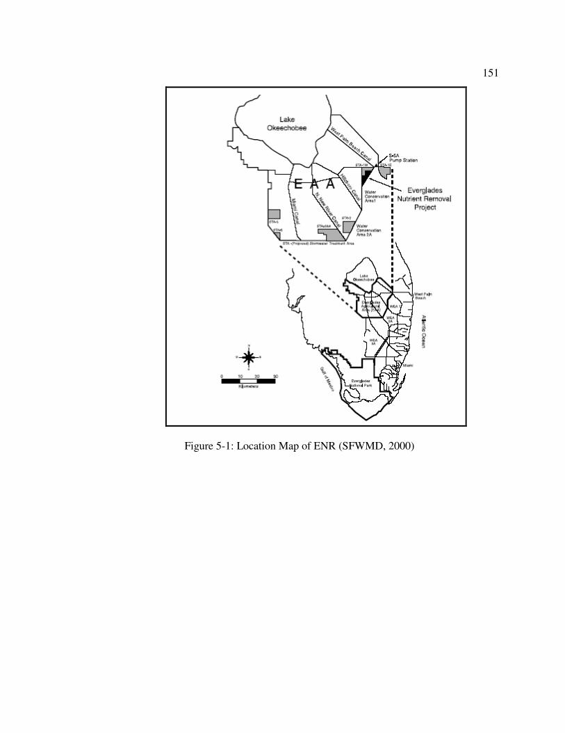
151
Figure 5-1: Location Map of ENR (SFWMD, 2000)
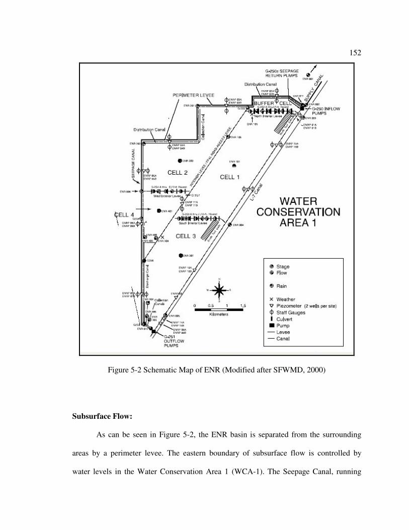
152
Figure 5-2 Schematic Map of ENR (Modified after SFWMD, 2000)
Subsurface Flow:
As can be seen in Figure 5-2, the ENR basin is separated from the surrounding
areas by a perimeter levee. The eastern boundary of subsurface flow is controlled by
water levels in the Water Conservation Area 1 (WCA-1). The Seepage Canal, running
153
along the western and northern boundary, controls the remaining boundaries. The bottom
boundary can be considered impermeable, since the field studies have found that
groundwater flow in the surficial aquifer is predominantly horizontal. Generally,
groundwater received a recharge from the WCA-1, where the water levels were normally
regulated between 4.88 m NGVD to 5.18 m NGVD (16 –17 ft NGVD), while discharge
was mainly through the seepage canal. Subsurface flow also received recharge through
overland flow infiltration.
Surface water flow in the ENR basin is controlled by a series of pump stations
and gated culverts. The ENR consists of a buffer cell and four treatment cells 1-4 (Figure
5-1). Stormwater runoff was pumped into the buffer cell and distributed to the eastern
flow way (Cell 1 and Cell 3) and the western flow way (Cell 2 and Cell 4). Interior levees
separated each treatment cell from one another and a series of culverts with risers were
built in the interior levees to control flows among cells. Treated water from the western
flow way was directed to Cell 3 by the gated culverts G-256 and eventually, was
discharged from ENR into WCA-1 through the outflow pump station G-251.
The major surface water inflow and outflow are through pumping stations G-250
and G-251. Structure inflows consisted of inflow pump station G-250 and seepage return
pump G-250S. Structure outflow was through outflow pump station G-251. Discharge
into the seepage canal could be made through gated structures G-258 and G-259. Current
modeling study simulated the whole calendar year of 1998. During this time period,
outflow from G-258 and G-259 was zero.
154
5.3 Model Tool: WASH123D
This is a generic, integrated surface water/groundwater interaction model code
(Yeh et al., 2006). It can simulate a one-dimensional channel network, two-dimensional
overland flows, and three-dimensional variably saturated subsurface flow, separately.
When needed, it can also simulate different combinations of coupled surface water and
subsurface water flows.
Some adaptations and modifications were easily implemented into the source
code for this modeling effort. The original WASH123D code apply constant friction
coefficient (Manning’s n value) for bottom shear stresses. But the dense vegetation in the
marsh area requires a water depth dependent Manning’s n relationship. Different depth
dependent relationships can be easily applied by a tabular (depth-n) profile input in
WASH123D.
The calibrated flow rating equations for various hydraulic structures can also be
coded in WASH123D that control the water transfer between different canal locations or
from/to canal to overland (marsh area).
5.4 Input Data
Time series data of rainfall, evapotranspiration, structure flow, and surface and
ground water levels were retrieved from the public accessible DBHYDRO database
(SFWMD, 2005).
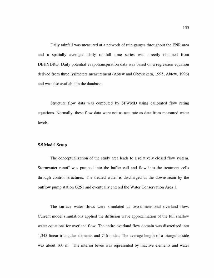
155
Daily rainfall was measured at a network of rain gauges throughout the ENR area
and a spatially averaged daily rainfall time series was directly obtained from
DBHYDRO. Daily potential evapotranspiration data was based on a regression equation
derived from three lysimeters measurement (Abtew and Obeysekera, 1995; Abtew, 1996)
and was also available in the database.
Structure flow data was computed by SFWMD using calibrated flow rating
equations. Normally, these flow data were not as accurate as data from measured water
levels.
5.5 Model Setup
The conceptualization of the study area leads to a relatively closed flow system.
Stormwater runoff was pumped into the buffer cell and flow into the treatment cells
through control structures. The treated water is discharged at the downstream by the
outflow pump station G251 and eventually entered the Water Conservation Area 1.
The surface water flows were simulated as two-dimensional overland flow.
Current model simulations applied the diffusion wave approximation of the full shallow
water equations for overland flow. The entire overland flow domain was discretized into
1,345 linear triangular elements and 746 nodes. The average length of a triangular side
was about 160 m. The interior levee was represented by inactive elements and water
156
could go only through it by structure flows. The known Inflow pumping rate was applied
by a water source term in the overland domain. A specified stage boundary condition
was applied at the downstream outflow location (G-251 headwater).
Vegetations were built into the treatment cells (Figure 5-3). They are categorized
as emergent cattails and submerged aquatic vegetation (SAV). Previous studies have
demonstrated that a water depth dependent friction coefficient is appropriate for
vegetation (Yen, 1992; Wu et al., 1999). Field study at ENR showed that the Manning’s n
values range from 0.5 to 1.3 depending on water depth and submergence level of the
plants (SFWMD, 2000).
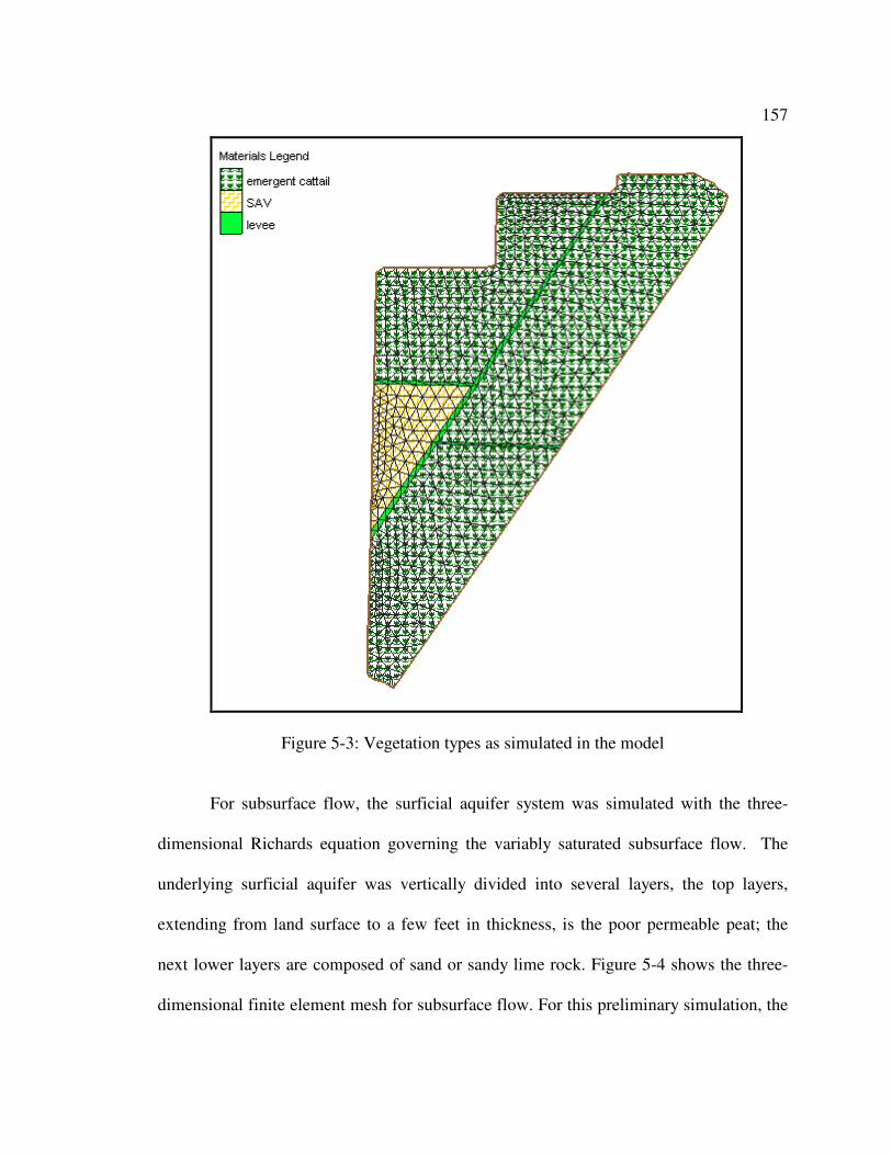
157
Figure 5-3: Vegetation types as simulated in the model
For subsurface flow, the surficial aquifer system was simulated with the three-
dimensional Richards equation governing the variably saturated subsurface flow. The
underlying surficial aquifer was vertically divided into several layers, the top layers,
extending from land surface to a few feet in thickness, is the poor permeable peat; the
next lower layers are composed of sand or sandy lime rock. Figure 5-4 shows the three-
dimensional finite element mesh for subsurface flow. For this preliminary simulation, the
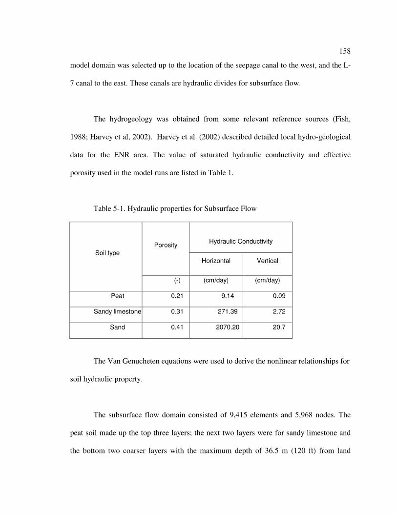
158
model domain was selected up to the location of the seepage canal to the west, and the L-
7 canal to the east. These canals are hydraulic divides for subsurface flow.
The hydrogeology was obtained from some relevant reference sources (Fish,
1988; Harvey et al, 2002). Harvey et al. (2002) described detailed local hydro-geological
data for the ENR area. The value of saturated hydraulic conductivity and effective
porosity used in the model runs are listed in Table 1.
Table 5-1. Hydraulic properties for Subsurface Flow
Hydraulic Conductivity Porosity
Horizontal Vertical
Soil type
(-) (cm/day) (cm/day)
Peat 0.21 9.14 0.09
Sandy limestone 0.31 271.39 2.72
Sand 0.41 2070.20 20.7
The Van Genucheten equations were used to derive the nonlinear relationships for
soil hydraulic property.
The subsurface flow domain consisted of 9,415 elements and 5,968 nodes. The
peat soil made up the top three layers; the next two layers were for sandy limestone and
the bottom two coarser layers with the maximum depth of 36.5 m (120 ft) from land
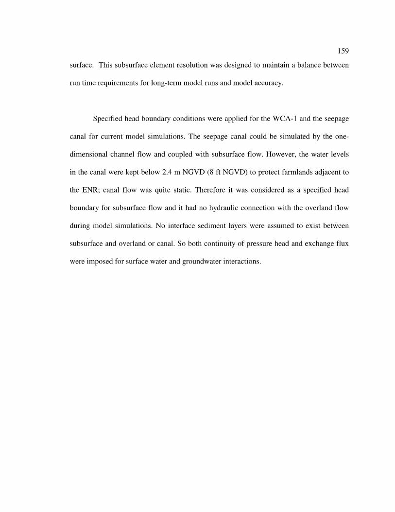
159
surface. This subsurface element resolution was designed to maintain a balance between
run time requirements for long-term model runs and model accuracy.
Specified head boundary conditions were applied for the WCA-1 and the seepage
canal for current model simulations. The seepage canal could be simulated by the one-
dimensional channel flow and coupled with subsurface flow. However, the water levels
in the canal were kept below 2.4 m NGVD (8 ft NGVD) to protect farmlands adjacent to
the ENR; canal flow was quite static. Therefore it was considered as a specified head
boundary for subsurface flow and it had no hydraulic connection with the overland flow
during model simulations. No interface sediment layers were assumed to exist between
subsurface and overland or canal. So both continuity of pressure head and exchange flux
were imposed for surface water and groundwater interactions.
160
Figure 5-4: Finite Element Meshes for ENR Basin with Soil Types
5.6 Model Calibration and Validation
The integrated model was calibrated and validated with both historic stage and
groundwater level data. Theoretically, most model parameters in a physics-based model
are measurable physical properties and can be estimated through field studies. The ENR
field studies (e.g. Harvey et al., 2002 and SFWMD, 2000) provided the physical range for
saturated hydraulic conductivity and the Manning’s roughness coefficient. However, due
to spatial heterogeneity and limited sampling sites, minimum model calibration is still
161
needed to better capture historic trends and this represent the averaging and upscale
uncertainty from point sampling to element level.
The split sample approach was used to calibrate and validate the ENR model.
The time period from 7/1/1998 to 12/31/1998 was used for model calibration and the
period from 1/1/1998 to 6/30/1998 was used in model validation. The model parameters
used in model calibration were the Manning’s roughness coefficient for overland flow
and the hydraulic conductivity for subsurface flow. The initial conditions for model
calibration and validation were estimated from observed surface water levels, flow rate
and groundwater levels.
The model performance was judged by mean error, absolute mean error, and root
mean square error, R2
and U2, between observed and computed time-series stages and
groundwater levels.
5.7 Model Simulation Results
The preliminary model simulation results (from 1/1/1998 to 12/31/1998) are
presented and discussed as follows. The average hydraulic conductivity values from field
studies (Table 5-1) were used for subsurface flow and no adjustment has been made. The
adjusted Manning’s roughness coefficients ranged from 0.3 to 0.9 for different
vegetations.
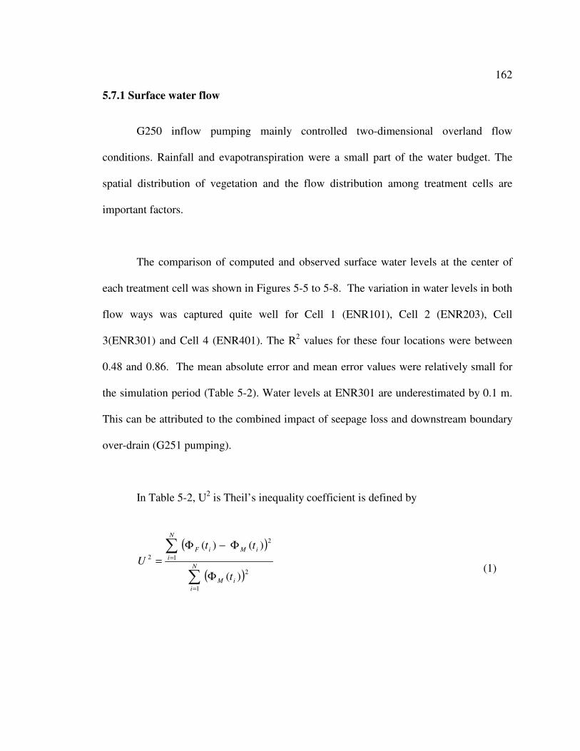
162
5.7.1 Surface water flow
G250 inflow pumping mainly controlled two-dimensional overland flow
conditions. Rainfall and evapotranspiration were a small part of the water budget. The
spatial distribution of vegetation and the flow distribution among treatment cells are
important factors.
The comparison of computed and observed surface water levels at the center of
each treatment cell was shown in Figures 5-5 to 5-8. The variation in water levels in both
flow ways was captured quite well for Cell 1 (ENR101), Cell 2 (ENR203), Cell
3(ENR301) and Cell 4 (ENR401). The R2 values for these four locations were between
0.48 and 0.86. The mean absolute error and mean error values were relatively small for
the simulation period (Table 5-2). Water levels at ENR301 are underestimated by 0.1 m.
This can be attributed to the combined impact of seepage loss and downstream boundary
over-drain (G251 pumping).
In Table 5-2, U2 is Theil’s inequality coefficient is defined by
( )
( )∑
∑
=
=
Φ
Φ−Φ
=N
i
iM
N
i
iMiF
t
tt
U
1
2
1
2
2
)(
)()(
(1)
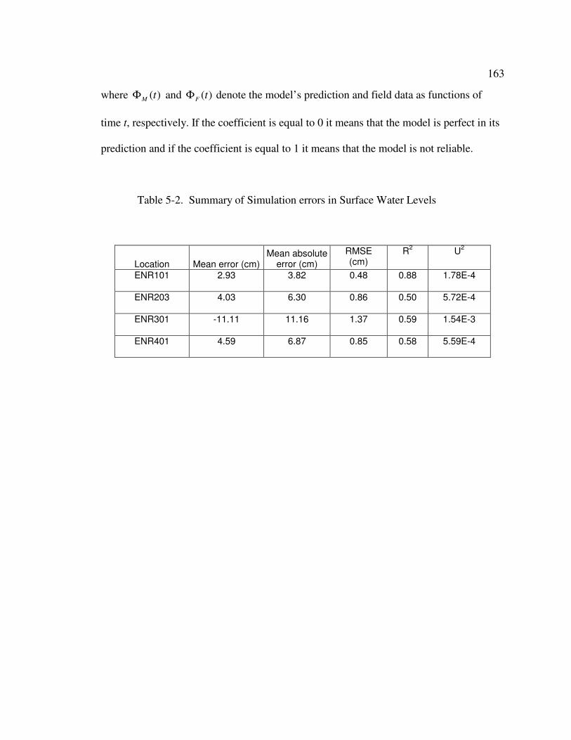
163
where )(tMΦ and )(tFΦ denote the model’s prediction and field data as functions of
time t, respectively. If the coefficient is equal to 0 it means that the model is perfect in its
prediction and if the coefficient is equal to 1 it means that the model is not reliable.
Table 5-2. Summary of Simulation errors in Surface Water Levels
Location Mean error (cm) Mean absolute
error (cm)
RMSE (cm)
R2 U
2
ENR101 2.93 3.82 0.48 0.88 1.78E-4
ENR203 4.03 6.30 0.86 0.50 5.72E-4
ENR301 -11.11 11.16 1.37 0.59 1.54E-3
ENR401 4.59 6.87 0.85 0.58 5.59E-4
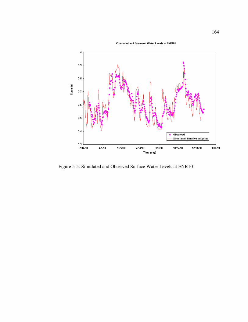
164
Figure 5-5: Simulated and Observed Surface Water Levels at ENR101
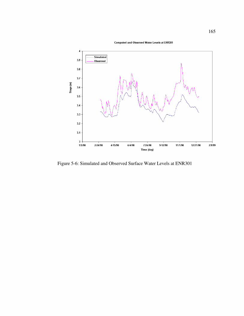
165
Figure 5-6: Simulated and Observed Surface Water Levels at ENR301
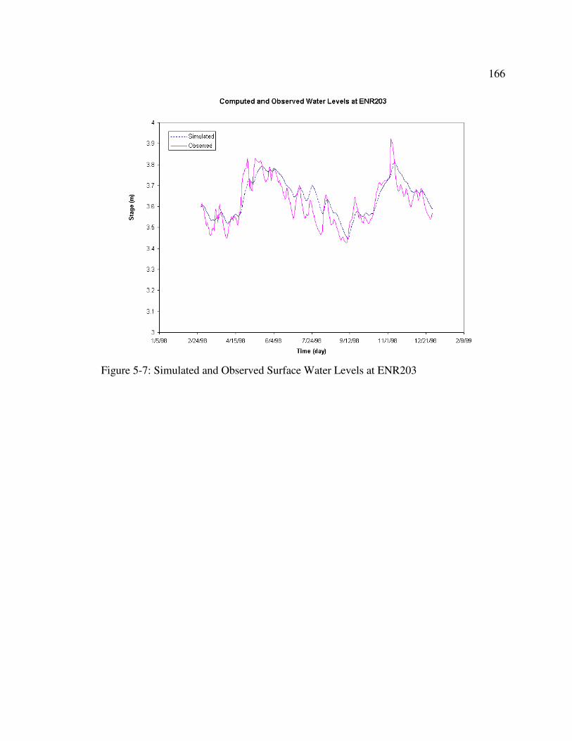
166
Figure 5-7: Simulated and Observed Surface Water Levels at ENR203
167
Figure 5-8: Simulated and Observed Surface Water Levels at ENR401
5.7.2 Subsurface Flow
The observed and computed groundwater levels at ENR102GW, ENR204GW,
ENR401GW and ENR303GW are compared in Figures 5-9 through 5-12. The simulation
results are similar to those of surface water levels. The average absolute error was less
than 8.5 cm. The simulation errors are summarized in Table 5-3.
168
Table 5-3. Summary of Simulation errors in Groundwater Levels
Location Mean error (cm) Mean absolute
error (cm)
RMSE (cm)
R2 U
2
ENR102GW 7.30 7.60 0.85 0.84 5.69E-4
ENR203GW 2.74 6.33 0.80 0.51 4.92E-4
ENR303GW 1.30 6.5 0.66 0.52 5.70E-4
ENR401GW 6.40 8.20 1.01 0.49 7.89E-4
The unsaturated zone was thin and localized during the simulation period. During
the dry season, a large portion of the surface area could dry up and soil moisture could be
less than saturated; under this flow condition, use of the Richards equation for variably
saturated subsurface flow in the model is justified. As a matter of fact, previous SFWMD
STA water budget studies (Huebner, 2001) applied a regression equation to account for
soil water storage during dry seasons.
The total head distribution on 2/4/1998 was plotted in Figures 5-13 through 5-15.
The simulated flow pattern of subsurface flow is consistent with field studies.
169
Figure 5-9: Simulated and Observed Groundwater Levels at ENR102GW
170
Figure 5-10: Simulated and Observed Groundwater Levels at ENR303GW
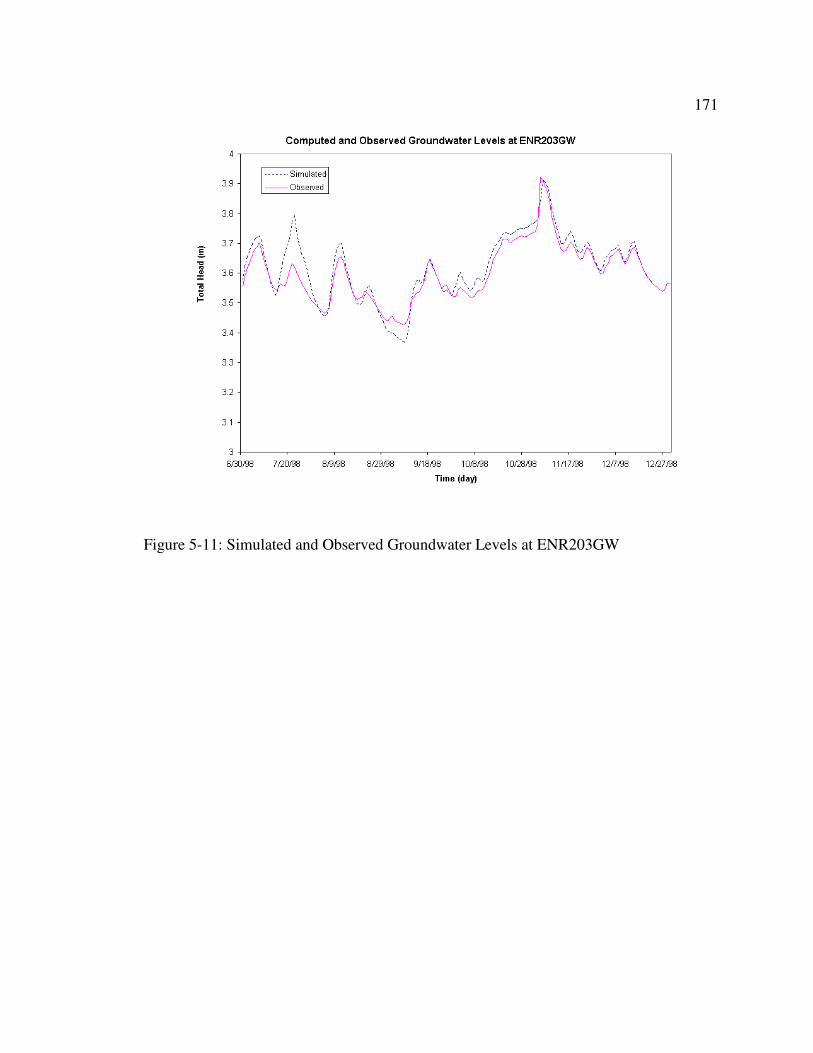
171
Figure 5-11: Simulated and Observed Groundwater Levels at ENR203GW
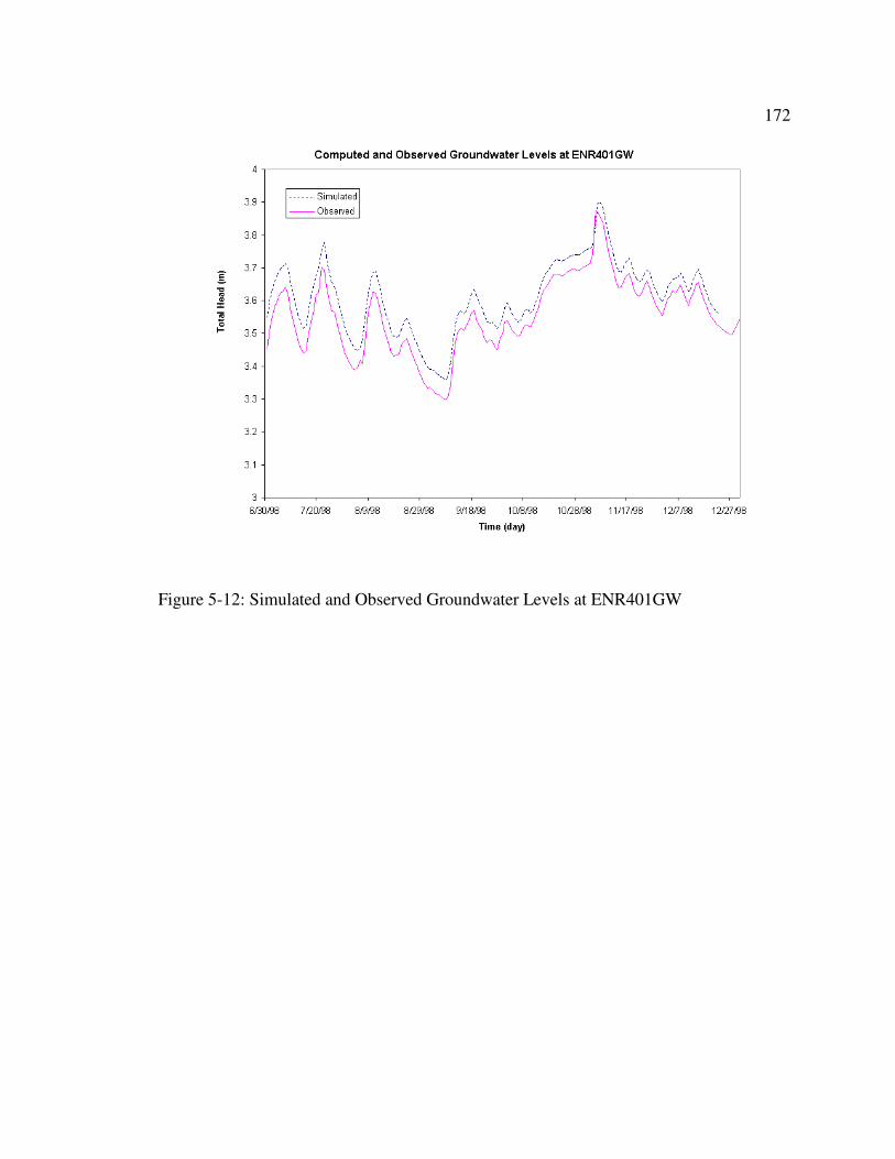
172
Figure 5-12: Simulated and Observed Groundwater Levels at ENR401GW
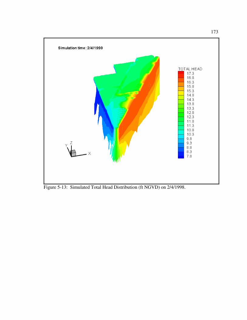
173
Figure 5-13: Simulated Total Head Distribution (ft NGVD) on 2/4/1998.
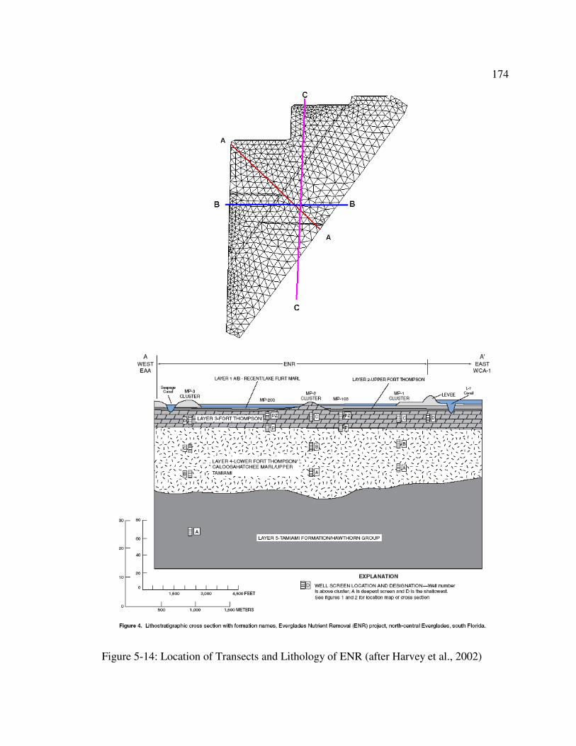
174
Figure 5-14: Location of Transects and Lithology of ENR (after Harvey et al., 2002)
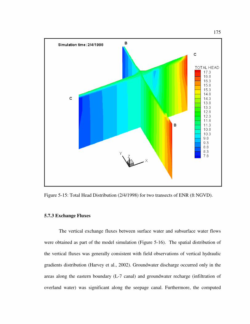
175
Figure 5-15: Total Head Distribution (2/4/1998) for two transects of ENR (ft NGVD).
5.7.3 Exchange Fluxes
The vertical exchange fluxes between surface water and subsurface water flows
were obtained as part of the model simulation (Figure 5-16). The spatial distribution of
the vertical fluxes was generally consistent with field observations of vertical hydraulic
gradients distribution (Harvey et al., 2002). Groundwater discharge occurred only in the
areas along the eastern boundary (L-7 canal) and groundwater recharge (infiltration of
overland water) was significant along the seepage canal. Furthermore, the computed
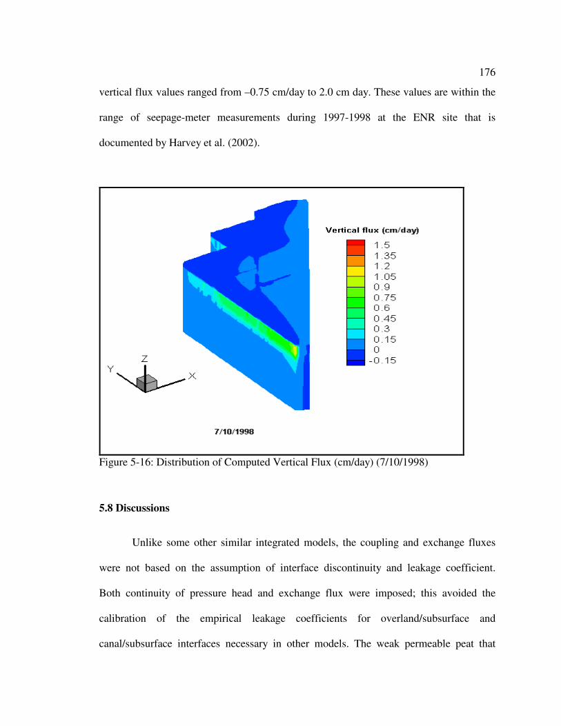
176
vertical flux values ranged from –0.75 cm/day to 2.0 cm day. These values are within the
range of seepage-meter measurements during 1997-1998 at the ENR site that is
documented by Harvey et al. (2002).
Figure 5-16: Distribution of Computed Vertical Flux (cm/day) (7/10/1998)
5.8 Discussions
Unlike some other similar integrated models, the coupling and exchange fluxes
were not based on the assumption of interface discontinuity and leakage coefficient.
Both continuity of pressure head and exchange flux were imposed; this avoided the
calibration of the empirical leakage coefficients for overland/subsurface and
canal/subsurface interfaces necessary in other models. The weak permeable peat that
177
restricts vertical subsurface flow was part of the subsurface domain. The model
simulation results in term of surface water levels, groundwater table, exchange fluxes,
etc. demonstrate that this coupling approach is aligned to the physical processes of the
ENR hydrology.
Details, in terms of variables such as vegetation type, local remnant ditches in the
marsh, culvert flow computation, etc., could more accurately model two-dimensional
overland flow. A dynamic wave model of overland flow, to replace the diffusion wave
approximation and the use of high-resolution time series data (e.g. 15 minute observed
data instead of daily average data used in current model simulations), may better simulate
the high-frequency dynamic variation. Although the simulation results show that
diffusion wave approximation is sufficient for overland flow.
5.9 Summary and Conclusions
A physics-based, integrated model was developed to simulate complex hydrologic
processes in a constructed wetland. The surface water and groundwater interactions were
simulated by coupled two-dimensional overland flow and three-dimensional subsurface
flow. Minimum model calibrations, combined with model parameters estimated from
field studies were able to reproduce major trends in historic surface and groundwater
levels. And the model provides details spatial distribution of state variables and fluxes.
178
Acknowledgements
The background information of STA-1W was provided by SFWMD through the
contract with Sutron Corporation (C-15988-WO04-05). The second author is supported
by the U.S. EPA - Science To Achieve Results (STAR) Program under Grant # R-
82795602 with the University of Central Florida.
References
Abtew,W. 1996. Evapotranspiration measurements and modeling for three wetland
systems in South Florida. Journal of the American Water Resources Association 32:
465-473.
Abtew, W. and J. Obeysekera. 1995. Lysimeter study of evapotranspiration of cattails
and comparison of three estimation methods. Transactions of the ASAE 38: 121-129.
Feng K. and Molz F.J. 1997. A 2-D, diffusion-based, wetland flow model. Journal of
Hydrology. 196 (1997) 230–250.
Fish, J.E., 1988, Hydrogeology, aquifer characteristics, and ground-water flow of the
Surficial Aquifer system, Broward County, Florida: U.S. Geological Survey Water
Resources Investigations Report 87-4034, 92 p.
179
Guardo, M. 1999. Hydrologic balance for a subtropical treatment wetland constructed for
nutrient removal: Ecological Engineering, V. 12, P. 315-337.
Guardo M. and Tomasello, R.S., 1995. Hydrodynamic simulations of a constructed
wetland in south Florida: Water Resources Bullrtin, v. 81, no.4, p. 687-701.
Huebner, S.R., 2001. Water Budget analysis for stormwater Treatment area 6, section 1,
Technical Publication EMA #391. South Florida Water Management District, West
Palm Beach, FL. February 2001.
Harvey, J.W., et. Al, 2002, Interactions between Surface Water and Ground Water and
Effects on Mercury Transport in the North-central Everglades: U.S. Geological Survey
Water Resources Investigations Report 02-4050, 91 pages.
Langevin C., Swain E., and Wolfert M., 2005. Simulation of integrated surface-
water/ground-water flow and salinity for a coastal wetland and adjacent estuary.
Journal of Hydrology. Volume 314, Issues 1-4, 25 November 2005, Pages 212-234.
South Florida Water Management District (SFWMD), 2000. 2000 Everglades
Consolidated Report, Chapter 6: Stormwater Treatment Areas. West Palm Beach, FL
SFWMD. 2005. DBHYDRO: http://www.sfwmd.gov/org/ema/dbhydro/index.html
Thompson J.R., H. Refstrup Sørenson, H. Gavin, A. Refsgaard. (2004). Application of
the coupled MIKE SHE/MIKE 11 modelling system to a lowland wet grassland in
southeast England. Journal of Hydrology. 293 (2004) 151–179.
180
Swain E.D., Melinda A. Wolfert, Jerad D. Bales, and Carl R. Goodwin, 2004. Two-
Dimensional Hydrodynamic Simulation of Surface-Water Flow and Transport to
Florida Bay through the Southern Inland and Coastal Systems (SICS). U.S.Geological
SurveyWater-Resources Investigations Report 03-4287, 2004.
Wu F., Shen H.W. and Chou Y. , 1999. Variation of Roughness Coefficients for
Unsubmerged and Submerged Vegetations., ASCE Journal of Hydolrogic Engineering,
Vol. 125, No. 9, September 1999.
Yeh, G.T., G. B. Huang, H. P. Cheng, F. Zhang, H. C. Lin, E. Edris, and D. Richards.
2006. Chapter 9: A first principle, physics-based watershed model: WASH123D, in
Watershed Models. Eds. By Singh VP and Frevert, CRC Press, Boca Raton, FL.
Yen, B. C., 1992. ‘‘Hydraulic resistance in open channels.’’ Channel flow resistance:
Centennial of Manning’s formula, B. C. Yen, ed.,Water Resources Publications,
Littleton, Colorado.
181
Chapter 6
Summary and Conclusions
Several critical issues in the development of a first principle, physics-based
watershed model are presented in this thesis.
Firstly, the implementation of all options of dynamic wave, diffusive and
kinematic wave models for surface flow in a single model code are used to investigate the
applicability and accuracy of diffusion and kinematic wave approximation and from
numerical experiments, it is concluded that the use of kinematic wave model should be
limited to steep-slope mountainous watersheds and where downstream conditions are not
important; The accuracy of diffusion wave under very mild slope is not guaranteed as
flow dynamics and downstream boundary may play a key role; The dynamic wave model
should be mandated for strong dynamic flow cases (e.g., dam break type flow), and when
momentum fluxes are important compared to gravity force.
Secondly, the numerical solution of the fully dynamic wave model of two-
dimensional overland flow is difficult. The detail and capability of a characteristics-based
finite element method is discussed and demonstrated with several typical examples.
Numerical simulation of a dam break problem demonstrates the numerical solution is
sensitive to the choice of wave characteristic directions.

182
Thirdly, physics based coupling of surface water and subsurface flow is at the
core of a physics-based, integrated watershed model; different combinations of coupling
schemes are discussed and compared, and physics-based coupling approaches are
favored. The inaccuracy and error of time-lagged, decoupled approach are demonstrated
in several test examples.
Finally, the performance of the watershed model in the integrated modeling of a
local-scale, field application was demonstrated through the study of surface water and
groundwater interactions in a constructed wetland in south Florida.
Further work includes (1) a thorough, formal theoretical analysis of diffusive and
kinematic wave approximations under two-dimensional overland flow condition; (2) full
scale, rigorous test of the new integrated watershed model for hydrologic processes in a
natural experiment watershed with research quality field data; (3) expand the subsurface
flow module to include preferential flow in macro-pores and discrete fractures; (4) fully
couple with the mechanistic based water quality and sediment transport module.
VITA
Guobiao Huang
Education
Ph.D. Civil Engineering, Pennsylvania State University, 2006
M.S. Water Resources Engineering, Hohai University, 1990
B.S. Water Resources Engineering, Tsinghua University, 1987
Professional Experience
June 2003 – present Senior Water Resources Engineer, Sutron Corporation, West
Palm Beach, FL
June 2002 – June 2003 Hydrologic Modeler, Science Applications International
Corporation, Miami, FL
Jan 2001 – May 2002 Graduate Research Assistant, Department of Civil and
Environmental Engineering, University of Central Florida, FL
June 1999 – Dec 2000 Graduate Research Assistant, Department of Civil and
Environmental Engineering, Pennsylvania State University, PA
Aug 1990 – May 1999 Senior Engineer (after 1995), Nanjing Research Institute of
Hydrology and Water Resources, Ministry of Water Resources, Nanjing, China
Selected Publications
Gour-Tsyh Yeh and Guobiao Huang, Hwai-Ping Cheng, Fan Zhang, Hsin-Chi Lin, Earl
Edris and David Richards. 2005. “ A first principle, physics based watershed model:
WASH123D”, chapter 9 in the book: Watershed Models, eds. by Vijay Singh and Donald
Frevert, CRC Press, Boca Raton, FL. September 2005.
Guobiao Huang, Gour-Tsyh Yeh, “Modeling coupled surface water and groundwater
flows from storm events using WASH123D”, Proceedings of the 1st annual stormwater
management research symposium at Orlando, Florida, p.107-117. October 2004.
Guobiao Huang and Gour-Tsyh Yeh, 2002. " Numerical Simulation of Surface runoff
with Coupled Two- Dimensional Overland Flow and One-Dimensional Stream Network
Flow", proceedings of the XIV International Conference on Computational Methods in
Water Resources (CMWR2002), Netherlands. June 2002.
Guobiao Huang and Gour-Tsyh Yeh, "Development of a Numerical Watershed Model",
Proceedings of the XIII International conference on Computational Methods in Water
Resources (CMWR2000), Calgary, Canada, June 2000.