Embed Size (px)
Citation preview

Universita degli Studi di VeronaDipartimento di Informatica
DOTTORATO DI RICERCA IN INFORMATICACICLO XV
PHYSICS-BASED MODELS
FOR THE ACOUSTIC REPRESENTATION
OF SPACE IN VIRTUAL ENVIRONMENTS
Coordinatore: Prof. Vittorio MurinoSupervisore: Prof. Davide Rocchesso
Dottorando: Federico Fontana


- REVISED VERSION -March, 2003


A Rossella,alla sua disponibilita e comprensione


Contestualizzazione della ricercae riassunto dei contenuti
In questo lavoro sono state affrontate alcune questioni inserite nel tema piu generale dellarappresentazione di scene e ambienti virtuali in contesti d’interazione uomo-macchina, neiquali la modalita acustica costituisca parte integrante o prevalente dell’informazione com-plessiva trasmessa dalla macchina all’utilizzatore attraverso un’interfaccia personale multi-modale oppure monomodale acustica.
Piu precisamente e stato preso in esame il problema di come presentare il messaggioaudio, in modo tale che lo stesso messaggio fornisca all’utilizzatore un’informazione quantopiu precisa e utilizzabile relativamente al contesto rappresentato. Il fine di tutto cio e riuscirea integrare all’interno di uno scenario virtuale almeno parte dell’informazione acustica che lostesso utilizzatore, in un contesto stavolta reale, normalmente utilizza per trarre esperienzadal mondo circostante nel suo complesso. Cio e importante soprattutto quando il focusdell’attenzione, che tipicamente impegna il canale visivo quasi completamente, e volto a uncompito specifico.
A tutt’oggi lo stato dell’arte nella rappresentazione di scene acustiche virtuali carat-terizzate da specifici attributi acusto-spaziali, e contenenti oggetti in forma di sorgenti disuono in grado di interagire tra loro formando eventi acustici riconoscibili, non prevede untipo d’interazione tra sistema e utilizzatore di tipo diretto, in grado cioe di soddisfare a deirequisiti che possono essere riassunti nei due punti seguenti:
• la presenza di oggetti e/o eventi nella scena la cui interpretazione non richieda l’utilizzodi processi di tipo cognitivo superiore, se non addirittura un addestramento di tipopreliminare finalizzato alla comprensione del significato della scena stessa;
• la possibilita di controllare in modo intuitivo e immediato gli oggetti e gli eventi nellascena, nonche i parametri acusto-spaziali caratterizzanti la scena nel suo complesso.
Da qualche tempo e in corso presso alcune comunita uno sforzo di ricerca per definiremetodi per la caratterizzazione acustica di oggetti ed eventi nella scena, attraverso unaloro realistica integrazione nel contesto. Queste ricerche fra l’altro hanno portato a modelliin grado di rappresentare fenomeni fisici corrispondenti a eventi salienti della scena stessa,quali ad esempio il rotolamento e lo schiacciamento di oggetti su una superficie, l’impatto elo sfregamento fra oggetti, la rottura eccetera.
i

E evidente che simili modelli soddisfano i requisiti espressi ai punti sopra. Infatti, lacomprensione dell’evento sonoro e in questi casi puramente ecologica, dunque immediata.Parimenti, il controllo degli stessi modelli e ben fondato e, di fatto, intuitivo, in quantodettato dalla dinamica del fenomeno fisico causante l’evento.
D’altra parte esiste la questione, accennata in precedenza, della contestualizzazione ditipo spaziale degli eventi appena descritti. In tal senso occorre ricordare che un soggettoudente percepisce la posizione angolare e la distanza degli oggetti relative alla posizioned’ascolto.
Contrariamente alla modellizzazione dei suoni emessi delle sorgenti acustiche, oggettodi ricerche riconducibili alla sintesi di suoni per l’interazione uomo-macchina, viceversa laspazializzazione delle stesse sorgenti, ovvero la loro collocazione nello spazio relativamenteal punto d’ascolto, e oggetto di studi di acustica e di psicoacustica volti a comprendere lemotivazioni psicofisiche della nostra percezione acustica dello spazio. Di conseguenza, pocoe stato fatto fino a questo momento per individuare dei modelli per la sintesi di attributispaziali, in grado di aggiungere all’informazione sulla natura degli oggetti della nuova infor-mazione, ancora oggettiva, volta alla specificazione della loro posizione nello spazio.
Un approccio basato sulla rappresentazione degli attributi acusto-spaziali dell’oggettosonoro trova un contesto applicativo qualificante in particolare nella riproduzione della dis-tanza tra oggetto e ascoltatore: rispetto a questo problema, infatti, e stato dimostrato chela componente soggettiva dovuta alla morfologia dell’ascoltatore riveste un ruolo percettivosecondario a confronto delle caratteristiche oggettive dello scenario. In altre parole, la ripro-duzione della distanza puo essere inglobata all’interno della rappresentazione dell’oggettoe, come tale, un modello volto a rappresentare acusticamente la distanza puo essere resosoggetto ai due requisiti inizialmente imposti.
Intendiamo dunque mettere a punto un modello per riprodurre acusticamente la distanzadegli oggetti sonori in una scena, il quale sia in grado di rappresentare l’informazione sulladistanza in modo immediatamente fruibile per l’utilizzatore. Nel contempo desideriamo chelo stesso modello sia controllabile in parametri di riscontro immediato.
E chiaro che il soddisfacimento di questi requisiti si traduce, a livello di prestazionidell’interfaccia, nella presenza di nuovi elementi informativi presenti nel canale audio, i qualideterminano un aumento assoluto della banda d’interazione disponibile e, piu in generale,un aumento del coinvolgimento dell’utilizzatore e del realismo dell’ambiente virtuale.
Il modello e stato realizzato supponendo di disporre di un tradizionale sistema per per-sonal computer per la presentazione dell’audio, in normali condizioni di utilizzo dell’interfaccia,e tenendo conto del modo in cui un soggetto normalmente udente e in grado di percepireacusticamente la distanza relativa dall’oggetto sonoro. I risultati ottenuti negli esperimentiattestano le promettenti prestazioni del modello sviluppato.
L’attesa disponibilta di parametri di controllo oggettivi ha richiesto di realizzare il mod-ello adottando uno schema numerico particolarmente adatto alla simulazione di domini dipropagazione d’onda distribuiti nello spazio tridimensionale, chiamato Waveguide Mesh.L’adattamento dello schema alle condizioni imposte dal modello si e tradotto in una se-
ii

rie di modifiche ad hoc e di migliorie apportate allo schema stesso, nell’ottica di una suaottimizzazione alla rappresentazione dell’ambiente virtuale proposto.
In parallelo, sono state studiate anche alcune problematiche di produzione e di presen-tazione dell’audio nell’interfaccia. Per quanto riguarda la produzione si e addivenuti a unmodello per la sintesi di eventi di fratturazione, utile alla generazione di suoni ecologici qualiil calpestio e lo schiacciamento. Per quanto riguarda la presentazione e stato messo a puntoun sistema innovativo per la realizzazione di funzioni di equalizzazione inversa, utile nellarimozione di artefatti presenti nel segnale audio dovuti a distorsioni causate dal sistemadi presentazione del messaggio acustico e dall’ambiente d’ascolto in cui lo stesso messaggioviene presentato.
Piu precisamente, gli elementi innovativi contenuti in questo lavoro sono riassumibili neipunti seguenti:
• e stata portata a termine un’analisi spazio-temporale della Waveguide Mesh, in con-seguenza della quale e stato possibile determinare la banda utile dei segnali ottenuticome risposta dello schema numerico al variare della geometria del reticolo, anche nelcaso in cui il reticolo presenti delle lacune in corrispondenza dei suoi punti nodali;
• e stata modellata una versione modificata della Waveguide Mesh rettangolare, la qualeproduce risposte all’impulso contenenti la stessa quantita di informazione offerta dallerisposte del modello originale, pur necessitando di risorse di calcolo e di memoriadimezzate;
• e stata proposta un’interpretazione fisica dell’errore numerico, cosiddetto di disper-sione, prodotto dalla Waveguide Mesh. Detta interpretazione e basata su risultatiottenuti nello studio di strutture, note come cable networks, che costituiscono la con-troparte meccanica del modello;
• e stata fornita una parametrizzazione di modelli di filtri, noti come Digital Waveg-uide Filter, utili a modellare il bordo della Waveguide Mesh nel caso in cui si stianosimulando superfici di riflessione d’onda acustica reali;
• e stata studiata una formulazione di tipo “scattered” del bordo della Waveguide Meshutile alla modellizzazione delle riflessioni multiple d’onda, quali quelle che avvengononormalmente nelle superfici reali;
• e stata modificata la struttura della Waveguide Mesh triangolare in modo tale daminimizzarne l’errore di dispersione. Per inciso cio ha richiesto di risolvere da un puntodi vista generale il problema della propagazione di un segnale all’interno di una retelineare di filtri contenente cicli senza ritardo, notoriamente non calcolabili utilizzandole classiche procedure di elaborazione del segnale. Detta soluzione si traduce in unaprocedura che fornisce automaticamente il sistema implicito di equazioni derivato dallarete stessa;
iii

• e stata definita una classe di geometrie per una cavita tridimensionale risonante, inmodo da studiare gli aspetti percettivamente interessanti contenuti negli spettri dellerisposte ottenute dalla stessa cavita man mano che la sua geometria varia, lungo laclasse, dalla forma sferica alla forma cubica. Cio per indagare la percezione dellaforma degli oggetti a partire da indizi di tipo sonoro;
• e stato messo a punto un modello per la sintesi di indizi di profondita acustica, al finedi evocare in un soggetto il senso della distanza a partire da informazioni audio. Equesto il punto piu qualificante della ricerca svolta, nel quale sono stati compendiati ipunti precedenti;
• e stata portata a termine una campagna di esperimenti volta a valutare il modello perla resa della distanza in diverse condizioni d’ascolto, facendo uso ora di cuffie audio,ora di altoparlanti. Da questi esperimenti sono emersi risultati incoraggianti, tali dalasciar intravedere un effettivo utilizzo del modello in interfacce uomo-macchina e inapplicazioni di realta virtuale di tipo convenzionale e avanzato;
• e stata sviluppata una struttura innovativa per una classe di filtri digitali nota comeequalizzatori parametrici, la cui specificita consiste nella semplicita d’inversione dellaloro funzione di trasferimento. Questa proprieta torna utile nella compensazione diechi e risonanze indesiderate contenute nel messaggio audio;
• desumendo la fisica della fratturazione da ricerche precedenti, si e addivenuti a unmetodo di sintesi di suoni particellari, la cui sovrapposizione secondo ben definiteregole statistiche ha permesso di sintetizzare suoni di calpestio e di schiacciamento.Il modello di sintesi ottenuto risulta controllabile in parametri di riscontro immediatoquali le dimensioni dell’oggetto schiacciato, la forza di schiacciamento e la resistenzadel materiale schiacciato. Attraverso l’uso di tale metodo si sono potuti definire deisuoni campione, successivamente applicati al modello per la resa della distanza per lacreazione di esempi audio opportuni.
La tesi, in lingua inglese, e stata organizzata in due parti. La prima parte contieneun’introduzione e un compendio generale del lavoro complessivo svolto. La seconda partepresenta in ordine cronologico alcuni lavori scritti dall’autore, pubblicati o sottoposti a revi-sione.
Attraverso questa organizzazione si e cercato di rendere piu agevole l’accesso al contenutocomplessivo anche al lettore meno interessato a entrare nello specifico dei singoli argomenti.Viceversa, il lettore desideroso di approfondire le tematiche proposte e invitato a considerareuna lettura della seconda parte.
Gli esempi audio sono proposti nel sito web dell’autore: www.sci.univr.it/∼fontana/ .
iv

Acknowledgments
It is impossible for me to acknowledge all the researchers I met during these years, forwhom I feel gratitude. Some of them are well-known personalities in their field, some othersare less present in the official boards. Independently of their position and visibility in thecommunity I found them to be as more engaging, as more sincerely involved in their researchtopic.
My first acknowledgments go to my early teachers and colleagues in Padua: GiovanniDe Poli, Roberto Bresin, Federico Avanzini, Nicola Orio, Carlo Drioli. And GianpaoloBorin, whose level of expertise in digital audio is far beyond the little number of preciouspublications and talks he gifted to our community.
I cannot forget the professional and human experience I had during my research visitat the Helsinki University of Technology. At the Laboratory of Acoustics and Audio SignalProcessing, for the first time in my life I was in a community where several researchers comingfrom different countries, cultures and backgrounds, having different positions in the academiaor the industry, working in multidisciplinary scientific fields with different levels of expertise,joined together to create a unique synergy. Matti, Mark, Vesa: I had exciting meetings andtalks with you, and I learned so much from your scientific, artistic and sometimes intuitivevision of sound. Cumhur, Hanna, Henri, Jyri, Lauri, Riitta, Ville: I would have just spentmore time with you. I deserve a special place in my mind for all the Aku guys and, more ingeneral, for Finland and its exotic atmosphere.
I cannot mention all my colleagues in Verona. Vittorio Murino, Andrea Fusiello, ManueleBicego, Laura Ottaviani, just to cite those with whom I was mostly in touch. I had occasionsto go beyond the scientific discussion with Linmi, Matthias and Umberto, whose guest roomsbecame invaluable for me more than one time. I had discussions of real computer sciencewith Vincenzo Manca and Roberto Giacobazzi. I would finally mention my PhD colleaguesand some of the research people in Verona: Alessandro, Arnaud, Debora, Giuditta, Graziano,Isabella, Nicola, and Nicola, for whom I hope the best. And Linda: I will never catch yourtheorems.
I supervised the graduation thesis of several students, both in Padua and in Verona. Ihope they enjoyed working with me in the subjects I proposed. Any one of them contributedto make a topic more clear or more difficult to understand: Luca, Enzo, Federico, Fabio,Giulio.
Monique Harris Muz translated in English the citations I added in the first part of the
v

thesis, at the beginning of each chapter. Zane Mackin gave me hints for improving theEnglish of the Preface and the Introduction and translated the citation at the beginning ofChapter 4, whose source in English I was unable to recover.
And, finally, I cannot forget the people I met during the international activities of ourgroup. I used to interact with them in an exciting and often funny way: Nicola Bernardini,Mikael Fernstrom, Marco Trevisani, Giovanni Bruno Vicario. And Bruno, Massimo, Sophia,Eoin, Kjetil, Mark. And Balazs: you will always find a hot meal in Italy.
My last, and strongest thanks go to Davide Rocchesso. We start collaborating togetherwhen he was a PhD candidate and I was a puzzled student of engineering, and an enthusiasticdrummer. That time I started dealing with the audio applications of computer science. Ihope not to stop working on them in the years to come.
vi

Preface
[. . . ] disserto di dominanti e colori del suono, di un centro neutro permanentedal quale col suono apportava o levava energia a qualunque sostanza.Ma c’era un problema: il generatore funzionava solo quando c’era lui,
e Keely era geloso di quel segreto che accordava la materia allo spirito.Puo egli aver scoperto qualcosa ed essere incapace di esprimerla?
[Nikola Tesla, osservazione sul Globe Motor di J. E. Worrell Keely. 1889.]
[. . . ] he spoke of dominants and colors of sound, of a permanent neutral centrewhich he gave or took away energy from, with the sound to whatever substance.
But there was a problem: the generator worked only with him,and Keely was jealous of that secret which gave form to spirit.
May he have discovered something and not be able to express it?[Nikola Tesla, observation on the Globe Motor made by J. E. Worrell Keely. 1889.]
The first time I went to a conference of computer music, in 1995, I was amazed bythe many panels presenting papers on acoustics, psychoacoustics, audio signal processing,applied computer science and audio engineering, which addressed musical performance, theart of composition, the specification of ideal listening and the ways to achieve that ideal.This musical emphasis was demonstrated by the conference’s social event, normally includingan artistic performance such as a concert of contemporary music: I later realized that thiswas a must in most of those conferences.
In the science of sound there is a clear link between research and art that is less commonthan other disciplines.
The study of the everyday listening experience and its systematic1 inclusion as a branch ofresearch in sound is quite recent. Perhaps this new branch has not yet been totally acceptedby some research communities in the field. Obviously, during most of their lifetime humansuse the hearing system to acquire information from the external world, but they spend littletime appreciating the acoustical subtleties of state of the art technology such as high-endsound synthesis and reproduction equipment. Likewise, most of the researchers working inother disciplines focus on solving problems that, directly or not, concern practical matters;rarely do they deal with the artistic derivations of their research.
1and not necessarily artistic, as it has been happening since long time ago: think, for instance, of LuigiRussolo’s intonarumori [132, 46].
vii

Do we choose to do study in the everyday listening spectrum only because our methodsof investigation cannot deal with the artistic level of the hearing experience? At least twoarguments can be given to nullify that suspicion. First, most everyday sounds are so familiarto the listener that they can be hardly reproduced by a model accurately enough to cheatthe hearing system, if not the subject. Second, art must not be used to mystify fair researchresults, as it happens sometimes in this field.
To put it plainly, we would say that models that simulate everyday listening, includingthose reproducing the spatial location of a sound source, those synthesizing ecological sounds,and more generally those adding some sense of presence to a virtual scenario, are prone tomore criticism and severe evaluation compared, for instance, to models for the synthesis ofhybrid sounds or for the automatic generation of scores.
On the other hand most of those actually doing research in sound are (or were) soundpractitioners or expert music listeners, if not musicians, composers or professionals in themusical field. Those people ought to consider a different research point of view, wherequality is evaluated by means of psychophysical tests, and musical sounds are substitutedby ecological events such as bounces, footsteps, rolling, crushing and breaking sounds.
This is not an easy perspective to adopt, especially for those having a musical background.It is opinion of the author that accepting this new perspective will be a key step in helpingthe science of sound to achieve a prominent position among the most respected scientificdisciplines.
viii

Contents
Contestualizzazione della ricerca e riassunto dei contenuti i
Acknowledgments v
Preface vii
Contents ix
Introduction 1
1 Physics-Based Spatialization 51.1 Spatial cues . . . . . . . . . . . . . . . . . . . . . . . . . . . . . . . . . . . . 5
1.1.1 Binaural cues . . . . . . . . . . . . . . . . . . . . . . . . . . . . . . . 61.1.2 Monaural cues . . . . . . . . . . . . . . . . . . . . . . . . . . . . . . . 71.1.3 Distance cues . . . . . . . . . . . . . . . . . . . . . . . . . . . . . . . 81.1.4 The HRTF model . . . . . . . . . . . . . . . . . . . . . . . . . . . . . 101.1.5 Objective attributes . . . . . . . . . . . . . . . . . . . . . . . . . . . 11
1.2 Reverberation . . . . . . . . . . . . . . . . . . . . . . . . . . . . . . . . . . . 121.2.1 Perceptual effects of reverberation . . . . . . . . . . . . . . . . . . . . 131.2.2 Perceptually-based artificial reverberators . . . . . . . . . . . . . . . 131.2.3 Physically-oriented approach to reverberation . . . . . . . . . . . . . 151.2.4 Structurally-based artificial reverberators . . . . . . . . . . . . . . . . 16
1.3 Physics-based spatialization models . . . . . . . . . . . . . . . . . . . . . . . 171.3.1 Physically-informed auditory scales . . . . . . . . . . . . . . . . . . . 18
2 The Waveguide Mesh: Theoretical Aspects 212.1 Basic concepts . . . . . . . . . . . . . . . . . . . . . . . . . . . . . . . . . . . 24
2.1.1 Wave transmission and reflection in pressure fields and uniform plates 242.1.2 WM models . . . . . . . . . . . . . . . . . . . . . . . . . . . . . . . . 252.1.3 Digital Waveguide Filters . . . . . . . . . . . . . . . . . . . . . . . . 27
2.2 Spatial and temporal frequency analysis of WMs . . . . . . . . . . . . . . . . 292.2.1 Temporal frequencies by spatial traveling wave components . . . . . . 29
ix

2.2.2 The frequency response of rectangular geometries . . . . . . . . . . . 322.2.3 WMs as exact models of cable networks . . . . . . . . . . . . . . . . 33
2.3 Scattered approach to boundary modeling . . . . . . . . . . . . . . . . . . . 382.3.1 DWF model of physically-consistent reflective surfaces . . . . . . . . 392.3.2 Scattering formulation of the DWF model . . . . . . . . . . . . . . . 41
2.4 Minimizing dispersion: warped triangular schemes . . . . . . . . . . . . . . . 43
3 Sounds from Morphing Geometries 473.1 Recognition of simple 3-D resonators . . . . . . . . . . . . . . . . . . . . . . 483.2 Recognition of 3-D “in-between” shapes . . . . . . . . . . . . . . . . . . . . . 49
4 Virtual Distance Cues 514.1 WM model of a listening scenario . . . . . . . . . . . . . . . . . . . . . . . . 514.2 Distance attributes . . . . . . . . . . . . . . . . . . . . . . . . . . . . . . . . 534.3 Synthesis of virtual distance cues . . . . . . . . . . . . . . . . . . . . . . . . 53
5 Auditioning a Space 575.1 Open headphone arrangements . . . . . . . . . . . . . . . . . . . . . . . . . 595.2 Audio Virtual Reality . . . . . . . . . . . . . . . . . . . . . . . . . . . . . . . 60
5.2.1 Compensation of spectral artifacts . . . . . . . . . . . . . . . . . . . . 605.3 Presentation of distance cues . . . . . . . . . . . . . . . . . . . . . . . . . . . 62
6 Auxiliary work – Example of Physics-Based Synthesis 656.1 Crumpling cans . . . . . . . . . . . . . . . . . . . . . . . . . . . . . . . . . . 67
6.1.1 Synthesis of a single event . . . . . . . . . . . . . . . . . . . . . . . . 686.1.2 Synthesis of the crumpling sound . . . . . . . . . . . . . . . . . . . . 696.1.3 Parameterization . . . . . . . . . . . . . . . . . . . . . . . . . . . . . 716.1.4 Sound emission . . . . . . . . . . . . . . . . . . . . . . . . . . . . . . 72
6.2 Implementation as pd patch . . . . . . . . . . . . . . . . . . . . . . . . . . . 73
Conclusion 77
II Articles 81
List of Articles 83
A Online Correction of Dispersion Error in 2D Waveguide Meshes 85A.1 Introduction . . . . . . . . . . . . . . . . . . . . . . . . . . . . . . . . . . . . 85A.2 Online Warping . . . . . . . . . . . . . . . . . . . . . . . . . . . . . . . . . . 86A.3 Computational Performance . . . . . . . . . . . . . . . . . . . . . . . . . . . 89A.4 Conclusion . . . . . . . . . . . . . . . . . . . . . . . . . . . . . . . . . . . . . 91
x
B Using the waveguide mesh in modelling 3D resonators 93B.1 Introduction . . . . . . . . . . . . . . . . . . . . . . . . . . . . . . . . . . . . 93B.2 3D schemes . . . . . . . . . . . . . . . . . . . . . . . . . . . . . . . . . . . . 94B.3 Implementation . . . . . . . . . . . . . . . . . . . . . . . . . . . . . . . . . . 96B.4 Summary . . . . . . . . . . . . . . . . . . . . . . . . . . . . . . . . . . . . . 99
C Signal-Theoretic Characterization of Waveguide Mesh Geometries for Mod-els of Two–Dimensional Wave Propagation in Elastic Media 101C.1 Introduction . . . . . . . . . . . . . . . . . . . . . . . . . . . . . . . . . . . . 101C.2 Background . . . . . . . . . . . . . . . . . . . . . . . . . . . . . . . . . . . . 102
C.2.1 Digital Waveguides and Waveguide Meshes . . . . . . . . . . . . . . . 102C.2.2 Sampling Lattices . . . . . . . . . . . . . . . . . . . . . . . . . . . . . 106
C.3 Sampling efficiency of the WMs . . . . . . . . . . . . . . . . . . . . . . . . . 107C.3.1 WMs and Sampling Lattices . . . . . . . . . . . . . . . . . . . . . . . 107C.3.2 TWM vs SWM . . . . . . . . . . . . . . . . . . . . . . . . . . . . . . 108C.3.3 TWM vs HWM . . . . . . . . . . . . . . . . . . . . . . . . . . . . . . 109
C.4 Signal time evolution . . . . . . . . . . . . . . . . . . . . . . . . . . . . . . . 111C.5 Performance . . . . . . . . . . . . . . . . . . . . . . . . . . . . . . . . . . . . 112
C.5.1 Numerical example . . . . . . . . . . . . . . . . . . . . . . . . . . . . 114C.6 Conclusion . . . . . . . . . . . . . . . . . . . . . . . . . . . . . . . . . . . . . 115C.7 Acknowledgment . . . . . . . . . . . . . . . . . . . . . . . . . . . . . . . . . 116C.8 Appendix - Sampling of a signal traveling along an ideal membrane . . . . . 116
D A Modified Rectangular Waveguide Mesh Structure with Interpolated In-put and Output Points 119D.1 Introduction . . . . . . . . . . . . . . . . . . . . . . . . . . . . . . . . . . . . 119D.2 A Modified SWM . . . . . . . . . . . . . . . . . . . . . . . . . . . . . . . . . 120D.3 Interpolated Input and Output Points . . . . . . . . . . . . . . . . . . . . . . 123D.4 Conclusion . . . . . . . . . . . . . . . . . . . . . . . . . . . . . . . . . . . . . 126
E Acoustic Cues from Shapes between Spheres and Cubes 127E.1 Introduction . . . . . . . . . . . . . . . . . . . . . . . . . . . . . . . . . . . . 127E.2 From Spheres to Cubes . . . . . . . . . . . . . . . . . . . . . . . . . . . . . . 128E.3 Spectral Analysis . . . . . . . . . . . . . . . . . . . . . . . . . . . . . . . . . 130E.4 Conclusion . . . . . . . . . . . . . . . . . . . . . . . . . . . . . . . . . . . . . 133
F Recognition of ellipsoids from acoustic cues 135F.1 Introduction . . . . . . . . . . . . . . . . . . . . . . . . . . . . . . . . . . . . 135F.2 Geometries . . . . . . . . . . . . . . . . . . . . . . . . . . . . . . . . . . . . 137F.3 Simulations . . . . . . . . . . . . . . . . . . . . . . . . . . . . . . . . . . . . 137F.4 Cartoon models . . . . . . . . . . . . . . . . . . . . . . . . . . . . . . . . . . 140F.5 Model implementation . . . . . . . . . . . . . . . . . . . . . . . . . . . . . . 141
xi

F.6 Acknowledgments . . . . . . . . . . . . . . . . . . . . . . . . . . . . . . . . . 142
G A Structural Approach to Distance Rendering in Personal Auditory Dis-plays 143G.1 Introduction . . . . . . . . . . . . . . . . . . . . . . . . . . . . . . . . . . . . 143G.2 Acoustics inside a tube . . . . . . . . . . . . . . . . . . . . . . . . . . . . . . 146G.3 Modeling the listening environment . . . . . . . . . . . . . . . . . . . . . . . 147G.4 Model performance and psychophysical evaluation . . . . . . . . . . . . . . . 149G.5 Conclusion . . . . . . . . . . . . . . . . . . . . . . . . . . . . . . . . . . . . . 153G.6 Acknowledgments . . . . . . . . . . . . . . . . . . . . . . . . . . . . . . . . . 153
H A Digital Bandpass/Bandstop Complementary Equalization Filter withIndependent Tuning Characteristics 155H.1 Introduction . . . . . . . . . . . . . . . . . . . . . . . . . . . . . . . . . . . . 155H.2 Synthesis of the Bandpass Transfer Function . . . . . . . . . . . . . . . . . . 156H.3 Implementation of the Equalizer . . . . . . . . . . . . . . . . . . . . . . . . . 158H.4 Summary . . . . . . . . . . . . . . . . . . . . . . . . . . . . . . . . . . . . . 160
I Characterization, modelling and equalization of headphones 163I.1 Introduction . . . . . . . . . . . . . . . . . . . . . . . . . . . . . . . . . . . . 163I.2 Psychoacoustical aspects of headphone listening . . . . . . . . . . . . . . . . 164
I.2.1 Lateralization . . . . . . . . . . . . . . . . . . . . . . . . . . . . . . . 164I.2.2 Monaural cues . . . . . . . . . . . . . . . . . . . . . . . . . . . . . . . 165I.2.3 Theile’s association model . . . . . . . . . . . . . . . . . . . . . . . . 167I.2.4 Other effects . . . . . . . . . . . . . . . . . . . . . . . . . . . . . . . . 167I.2.5 Headphones vs. loudspeakers . . . . . . . . . . . . . . . . . . . . . . . 168
I.3 Types and modelling of headphones . . . . . . . . . . . . . . . . . . . . . . . 168I.3.1 Circumaural, supra-aural, closed, open, headphones . . . . . . . . . . 169I.3.2 Isodynamic, dynamic, electrostatic transducers . . . . . . . . . . . . . 170I.3.3 Acoustic load on the ear . . . . . . . . . . . . . . . . . . . . . . . . . 173
I.4 Equalization of headphones . . . . . . . . . . . . . . . . . . . . . . . . . . . 173I.4.1 Stereophonic and binaural listening . . . . . . . . . . . . . . . . . . . 173I.4.2 Conditions for binaural listening . . . . . . . . . . . . . . . . . . . . . 174I.4.3 Binaural listening with insert earphones . . . . . . . . . . . . . . . . 175
I.5 Conclusions . . . . . . . . . . . . . . . . . . . . . . . . . . . . . . . . . . . . 177
J Computation of Linear Filter Networks Containing Delay-Free Loops, withan Application to the Waveguide Mesh 179J.1 Introduction . . . . . . . . . . . . . . . . . . . . . . . . . . . . . . . . . . . . 179J.2 Computation of the Delay-Free Loop . . . . . . . . . . . . . . . . . . . . . . 181J.3 Computation of Delay-Free Loop Networks . . . . . . . . . . . . . . . . . . . 182
J.3.1 Detection of Delay-Free Loops . . . . . . . . . . . . . . . . . . . . . . 186
xii

J.4 Scope and Complexity of the Proposed Method . . . . . . . . . . . . . . . . 187J.5 Application to the TWM . . . . . . . . . . . . . . . . . . . . . . . . . . . . . 189
J.5.1 Reducing dispersion . . . . . . . . . . . . . . . . . . . . . . . . . . . 191J.5.2 Results . . . . . . . . . . . . . . . . . . . . . . . . . . . . . . . . . . . 192
J.6 Conclusion . . . . . . . . . . . . . . . . . . . . . . . . . . . . . . . . . . . . . 194J.7 Appendix . . . . . . . . . . . . . . . . . . . . . . . . . . . . . . . . . . . . . 195
J.7.1 Existence of the solutions . . . . . . . . . . . . . . . . . . . . . . . . 195J.7.2 Extension of the method to any linear filter network . . . . . . . . . . 196J.7.3 Detection of delay-free loops . . . . . . . . . . . . . . . . . . . . . . . 196
K Acoustic distance for scene representation 199K.1 Introduction . . . . . . . . . . . . . . . . . . . . . . . . . . . . . . . . . . . . 199K.2 Hearing distance . . . . . . . . . . . . . . . . . . . . . . . . . . . . . . . . . 201K.3 Absolute cues for relative distance . . . . . . . . . . . . . . . . . . . . . . . . 202K.4 Displaying auditory distance . . . . . . . . . . . . . . . . . . . . . . . . . . . 205K.5 Modeling the virtual listening environment . . . . . . . . . . . . . . . . . . . 206K.6 Model performance . . . . . . . . . . . . . . . . . . . . . . . . . . . . . . . . 210K.7 Psychophysical evaluation . . . . . . . . . . . . . . . . . . . . . . . . . . . . 212
K.7.1 Headphone listening . . . . . . . . . . . . . . . . . . . . . . . . . . . 212K.7.2 Loudspeaker listening . . . . . . . . . . . . . . . . . . . . . . . . . . . 213K.7.3 Discussion . . . . . . . . . . . . . . . . . . . . . . . . . . . . . . . . . 214
K.8 Conclusion and future directions . . . . . . . . . . . . . . . . . . . . . . . . . 215K.9 SIDEBAR 1 – Sonification and Spatialization: basic notions . . . . . . . . . 217K.10 SIDEBAR 2 – Characteristics of Reverberation . . . . . . . . . . . . . . . . 217K.11 SIDEBAR 3 – The Waveguide Mesh . . . . . . . . . . . . . . . . . . . . . . 219
Bibliography 223
xiii


Introduction
Qualora si voglia comprendere il senso delle trasformazioni realidell’attivita di progettazione (nel XX secolo) sara necessario
costruire una nuova storia del lavoro intellettuale e della sua lentatrasformazione in puro lavoro tecnico (in ‘lavoro astratto’, appunto).
[. . . ] Inutile piangere su un dato di fatto: l’ideologia si e mutatain realta, anche se il sogno romantico di intellettuali che
si proponevano di guidare il destino dell’universo produttivoe rimasto, logicamente, nella sfera sovrastrutturale dell’utopia.
[Manfredo Tafuri, La sfera e il labirinto: avanguardie e architettura da Piranesi agli anni ’70. 1980.]
Whenever you want to understand the sense of the real transformationsof the design activity (in the 20th century) it would be necessary
to create a new history of the intellect and of its slow transformationinto a pure technical job (into an ‘abstract job’, in fact).
[. . . ] It’s unnecessary to cry over a matter of fact: ideology muted into reality,even if the romantic dream of intellectuals, who proposed to lead the productive
universe’s destiny, still remains, logically, in the overall sphere of utopia.[Manfredo Tafuri, La sfera e il labirinto: avanguardie e architettura da Piranesi agli anni ’70. 1980.]
This work deals with the simulation of virtual acoustic spaces using physics-based models.The acoustic space is what we perceive about space using our auditory system. The physicalnature of the models means that they will present spatial attributes (such as, for example,shape and size) as a salient feature of their structure, in a way that space will be directlyrepresented and manipulated by means of them.
We want those models to be provided with input channels, where anechoic sounds canbe injected, and output channels, where spatialized sounds can be picked up. We alsoexpect that the spatial features of those models can be modified even during the simulation(namely, runtime) through the manipulation of proper tuning parameters, without affectingthe effectiveness of the simulation. Once these requirements are satisfied, we will use themodels as sound synthesizers and/or sound processors to provide anechoic sounds with spatialattributes, in the way expressed by Figure 1.
Finally, we will use our models as reference prototypes for the design of alternative,simplified representations of the auditory scene when such representations appear to bemore versatile than the original prototypes, especially for application purposes.
1

2 Physics-based models for the acoustic representation of space in virtual environments
MODEL
SPATIALIZATIONSpatialized Output
Spatial features
Anechoic Input
Figure 1: Spatialization model
As we will see in more detail in Chapter 1, sound spatialization (primarily concernedwith the representation of reverberant environments) has an important place in the historyof audio. Especially during past decades there has been some difficulty in adding convincingspatial attributes in real-time to sound. This has led to a large variety of solutions whichprovided satisfactory reverberation in the majority of cases.
On the other hand, the spatial attributes provided by those solutions were often qual-itative. In other words, most of the geometrical and structural figures characterizing thespatialization domain (such as the shape of a resonator, the size of an enclosure or theabsorption properties of walls) have rarely been considered worth rendering.
Indeed, the qualitative approach is supported by psychoacoustics. Since humans can onlyroughly evaluate structural quantities from spatialized sounds, any effort to design modelsthat can be tuned in the quantitative parameters would possibly result in applications whoseperformance does not justify their technical complexity. Nevertheless, this considerationapplies especially to musical listening contexts, where the salient features of the auditoryscene and the acoustic quality of the listening environment relate in a complicated andunpredictable way to the structural parameters of the physical environment.
Conversely, let us consider the everyday listening experience. There the auditory systemis engaged in different tasks, mainly recognition and evaluation. One of those, for example,is distance evaluation. For the aforementioned reasons, the traditional literature aboutspatialization by means of reverberation has not too much to share with those tasks.
There is a branch of the field of Human-Computer Interaction (HCI), called auditorydisplay, where the subjective evaluation of a listening scenario is seriously considered. Fromthe literature concerned with the psychophysics of human auditory localization we learn thatthere is a gap between the precision of the physical laws that calculate the sound pressurelevel in the vicinity of the listener’s ears, caused by the sonic emission from a sound sourcelocated somewhere in a listening environment, and the unpredictability of the listener’sjudgment about the spatial attributes of the same environment. We say that the perceivedspatial attributes differ from their corresponding objective quantities.
Due to its nature, a physics-based model for sound spatialization can be easily accommo-dated to simulate a listening environment whose attributes are conveyed to the listener in the

3
form of auditory spatial cues. Using that model we can reproduce those cues, manipulatingtheir properties by directly controlling the physical quantities that characterize the listeningenvironment.
The quality of the model will be evaluated through listening tests. We cannot keepsubjective differences under control, but this is not a major concern for this work, since weare not interested in tailoring models to optimize subjective performance. Conversely, wewant to validate those models by comparing the subjects’ overall subjective evaluations withresults found in alternative experiments conducted in real listening environments.
In one case concerning the auditory recognition of three-dimensional cavities, we haveused the model also as a reference listening environment, since we did not find psychophysicalexperiments in the literature to be taken as a reference counterpart.
Following a general introduction to sound spatialization in Chapter 1, Chapter 2 dealswith some preliminary theoretical facts about the Waveguide Mesh, the numerical schemewhich we will extensively use to give an objective representation of auditory space. Thischapter is interesting especially for those who are familiar with this scheme, although itscomprehension highlights the advantages and actual limits of the Waveguide Mesh as aspatialization tool.
In Chapter 3 we propose an example of sonification in between sound synthesis and soundspatialization. In this chapter, we will examine the motivations for synthesizing sounds frommodels of ideal resonant cavities, having shapes ranging from the sphere to the cube. We willalso show the method we have followed to simulate the aforementioned cavities, and discussthe results obtained by the corresponding simulations, along with their interpretation.
Chapter 4 describes a virtual listening environment for the synthesis of distance cuesrealized using the Waveguide Mesh. Due to its tubular design, this environment can beeasily constructed. Results of its evaluation are discussed basing on subjective ratings onthe effectiveness of the cues provided by that virtual environment. Those results indicatethat physics-based modeling can play a role in the design of spatialization tools devotedespecially to the presentation of information in multimodal human-computer interfaces.
Chapter 5 addresses the question of presenting auditory data. This chapter emphasizesthe problems that arise when spatialized sounds finally have to be presented to the listenerand the possible consequences of a wrong presentation, even using state-of-the-art reproduc-tion systems. Although the chapter does not break any new ground in this specific field, itnevertheless surveys some facts related to headphone presentation, and defines a frameworkin which our spatialization model can be successfully employed. Part of the chapter is de-voted to presenting a novel structure of parametric equalizers, useful for canceling the mostaudible artifacts coming from distortions caused by the audio chain and peculiar defects ofthe listening environment where the audio reproduction system is located.
Finally, it is our conviction that a model which simulates the acoustic space must processsounds coming from the everyday listening experience. For this reason, Chapter 6 of thiswork only briefly addresses the specification and synthesis of a certain type of ecologicalsound that we will call, with some generality, crumpling sound. Those sounds result from a

4 Physics-based models for the acoustic representation of space in virtual environments
superposition of individual bouncing events according to certain stochastic laws, in such away that varying the bouncing parameters and/or the stochastic law translates into a changeof the “nature” of the resulting sounds. Hence, they can represent the crushing of a can, ora single footstep. The results obtained in this chapter will be used as an autonomous set ofanechoic samples, to feed the spatialization models.
Whenever a careful treatment of at least part of a topic mentioned in any chapter canbe found, references will be given. In particular, articles already written or co-authoredby the same author of this work, covering the subjects proposed herein, will be reportedin the second part of the thesis. This choice has been made with the purpose of avoidingrearrangements and condensations of arguments that have already been presented, and tosave the reader from too much detail on any particular topic.
Nevertheless, an effort has been made to keep the first part of the thesis self-contained,in such a way that the general sense of the overall work can be understood from that part.Whenever needed the reader can refer to the second part.
Several audio examples have been produced using the tools developed during this work.Actually, they are meaningful only in an ongoing research process. For this reason, here weinclude the address of the author’s web site, where proper links to those examples can befound. This address is www.sci.univr.it/∼fontana/ .
Finally, a convention in the use of pronouns should be pointed here. We will refer tosubjects acting in a listening context (such as talkers) using feminine pronouns. On theother hand, listeners and, more in general, machine users will be identified with masculinepronouns.
Chapter 1
Physics-Based Spatialization
Gia a meta del Settecento Julien Offroy de La Mettrie descrivevane L’Homme-Machine la trasformazione del dualismo uomo-natura
in quello uomo-macchina, anche se l’assunzione del modello macchinacome spiegazione della realta fisica risale alla meta del XVII secolo.
[Vittorio Gregotti, Architettura, tecnica, finalita. 2002.]
By the middle of the Eighteenth century Julien Offroy de La Mettrie describedin the book “L’Homme-Machine” the transformation of the man-nature dualism
into man-machine dualism, even if the assumption of the machine modelas explanation of the physical reality, dates back to the middle of the Seventeenth century.
[Vittorio Gregotti, Architettura, tecnica, finalita. 2002.]
The only place to hear sounds that are unaffected by spatialization cues is the insideof a good anechoic chamber. In that listening situation, sound pressure waves either reachthe listening point or fade against the walls of the chamber. More precisely, both the soundsource and the listener should be as transparent to sound waves as possible. Ideally, both ofthem should be point-wise and have the same directivity and sensitivity along all directions.In all other cases, sounds are affected by some kind of spatialization.
1.1 Spatial cues
Consider the case of a group of persons talking inside an anechoic chamber: each speaker,in addition to her personal voice, has a direction-dependent emission efficiency (or directiv-ity), and diffracts the emitted acoustic waves with her head and body, so that, for example,she can be heard by listeners even if she does not face them. Each listener partially absorbs,partially reflects, and, in his turn, diffracts those waves before they reach the listeners’ ears.Objects which are present in the scene behave as reflectors and diffractors as well, and inaddition can transmit acoustic waves. Moreover, speakers are also listeners, so that theirpresence in the scene determines changes similar to those caused by the listeners. This pe-culiar example, referred to an anechoic chamber, shows that there are very few situations
5

6 Physics-based models for the acoustic representation of space in virtual environments
in which sounds are not spatialized, so that in almost all listening contexts humans can inprinciple extract spatial cues from sounds, that give information about the relative position,orientation and distance of the sound source, and about the listening environment.
Despite the existence of spatial information in the sounds, humans are not able to exploitthat information in a way that they can extract a precise scene description from it, butgrossly. In fact, spatial attributes contained in unfamiliar sounds in general do not translateinto reliable cues, such as loudness or pitch, that enable humans to perform precise detections[171]. An exception comes from the detection of the angular position of a sound source,that can be assessed even with good precision for certain sources. This happens due tobinaural listening, and due to the existence of the precedence effect, but not due to thespatial information that is inherently contained in the sound as it approaches the listener’sproximity.
To stay in the example of the talkers in the anechoic chamber, a listener can normallydetect the angular position of the speaker with good precision and, to some extent, recognizeher distance and her orientation inside the chamber given that her voice is familiar to him,i.e., once some prior training has been conducted inside the anechoic environment. He canalso detect the presence in the chamber of a large object if it has a sufficient reflectivity.
In the following of this chapter we will briefly survey human auditory spatial perception.In fact, a basic knowledge of spatial hearing cannot be avoided by the reader interested inthis work. Since excellent research has been done in the subject, the reader will be oftenreferred to the literature.
We will pay more attention in outlining the psychophysics of distance perception. In fact,one goal of this research is to provide models for the synthesis of virtual attributes of distance.Thus, a comprehension of the mechanisms enabling distance perception is considered to befundamental for the reader who wishes to capture the meaning of the following chapters,and the overall sense of this work.
1.1.1 Binaural cues
Binaural cues give humans a powerful way to detect the angular position of a soundsource. In fact, the hearing system is capable of processing the time differences of individuallow-frequency components contained in a sound, that reach the two ears at different arrivaltimes due to the interaural distance. These cues are known in the literature as InterauralTime Differences (ITD), and enable humans to position the sound source into a geometricallocus (the so-called cone of confusion) that is consistent with those time differences [15].
Moreover, the hearing system can also detect the intensity differences of individualmedium- and high-frequency components contained in a sound, that reach the two ears atdifferent amplitudes due to the masking effect caused by the head (also called head shadow).These cues, which are binaural as well, are known in the literature as Interaural IntensityDifferences (IID) or Interaural Amplitude Differences (IAD) [15].
ITD and IID are complemented by the precedence effect, by means of which binaural

Chapter 1. Physics-Based Spatialization 7
differences contained in signal onsets are taken in major consideration by the hearing system.As a consequence, the angular position of a sound source detected during the attack of asound is retained for a few tens of milliseconds, regardless of the positional informationcontained in the signal immediately following the onset [15, 124].
Head diffraction gives humans also the possibility, to some extent, to recognize the dis-tance of a sound source located in the near-field (that is, within about 1 m) [145, 22]. Thesynthesis of binaural cues providing near-field distance information is not object of study inthis work, for reasons that will be made clear in the following.
Binaural cues can be effectively reproduced by models that calculate the ITD and IIDaccording to the angular position of the sound source [21]. Those models in general leavesome degree of approximation in the reproduction of such cues: in fact, binaural cues aregenerally considered to be quite robust against subjective evaluation.
IID can also be modeled to reproduce the distance of a nearby source [41].
1.1.2 Monaural cues
Before reaching the ear canal, sound waves are processed by the human body. Torso,shoulders, and in particular the two (supposed identical) ear pinnas, add spatial cues to asound according to the subjective anthropometric characteristics of each individual. Thosecues do not bring independent information to each one of the two ears, hence they are calledmonaural1.
Moreover, during their path from the acoustic source to the listener’s proximity, soundsare modified by the listening environment. As we will see later in more detail the environmentis responsible for important modifications in the sound, which are grouped here togetherwith the monaural effects of the human body. Although from a physical viewpoint suchmodifications result in independent sounds reaching the two ears, the binaural differencesexisting in those “environmental” attributes do not convey binaural cues as well.
Monaural cues enable humans to recognize the elevation and distance of a sound source,along with other features which are not object of study in this work [166]. As a rule of thumb,cues caused by the listener’s body play a major role in the detection of the elevation, whereascues added by the environment are mainly responsible for distance evaluation. Despite this,environmental modifications mainly consisting in sound reflections over the floor have beenreported to convey elevation cues [68]. On the other hand, interferences caused by thehead against the direct sound originating from nearby sources have been hypothesized to beresponsible for monaural distance cues by Blauert [15].
It is straightforward to notice that monaural cues are less reliable than binaural cues.In fact, their existence in a sound can be detected by the hearing system as soon as thesource (i.e., free of monaural cues) sound is familiar to the listener [15]. For the same reason,dynamic changes in the sound source or the listener’s positions have positive effects in the
1Though, inequalities between the left and right side of the body, in particular pinna inequalities, havebeen reported to convey binaural cues accounting for elevation [141].

8 Physics-based models for the acoustic representation of space in virtual environments
detection of elevation and distance, since during those changes (that turn into variation inthe corresponding cues) the hearing system can familiarize with the original sound, and,thus, better identify the cues added by the listener’s body and the listening environment.
Monaural cues which are added by the body have a quite subtle dependency on thelistener’s anthropometric characteristics: for this reason they are highly subjective, andmuch more difficult to reproduce than binaural cues. Nevertheless, models exist aiming atevoking a sense of elevation [8, 3]. In general, these models tend to work better if they canhandle dynamic variations of the elevation parameters once they have been informed aboutthe listener’s head position [57].
For their importance in this work, monaural cues added by the listening environment aredealt with in the following section.
1.1.3 Distance cues
Distance detection involves the use of many (possibly all) monaural cues that are presentin a sound. In the simple case of one still sound source playing in a listening environmentin the medium- or far-field, our hearing system recognizes an auditory event to happensomewhere in the environment.
It is likely that the localization of the auditory event, in particular its distance fromthe listener, is somehow related with the actual position of the sound source. In the caseof distance perception, the gap existing between the position of the sound source and thelocalization of the auditory event is influenced by several factors, and in many cases itcannot be easily explained or satisfactorily motivated. Judgments on distance are influencedby visual cues as well [144].
Also, the so-called distance localization blur [15] has been discovered to be non-negligible,main consequence of the subjectivity of the psychophysical scales on which subjects relyduring the evaluation.
In general, psychophysical tests investigating distance perception are difficult to designand set up, sometimes contradicting, and (especially in the case of prior investigations) oftenprone to criticism on the methodological approach, and suspicion concerning the quality ofthe equipment used for the tests [15].
Experiments aiming at studying the effects of one singular cue, although keeping a highdegree of control over the test, led sometimes to results having low practical consequences.Nevertheless, those experiments have shown that three monaural cues are important fordistance perception [167]:
loudness – this cue plays a fundamental role especially in the open space, and once thesound source is familiar to the listener (the last fact is frequently expressed in theliterature saying that loudness is a relative distance cue). In an ideal open space oranechoic environment, each doubling of the source/listener distance causes the soundpressure at the listener’s ear to decrease by 6 dB [102]. Hence, if the source emits afamiliar sound (particularly speech), then the hearing system is capable of locating the

Chapter 1. Physics-Based Spatialization 9
auditory event based on the loudness resulting from the corresponding sound pressureat the ear entrance.
Experiments where the pressure at the ear canal was kept under control have shownthat the logarithmic distance of the auditory event is mapped by the sound pressurevalue at the ear, measured in dB, according to an approximatively linear psychophys-ical law—at least within specific ranges and for some sound sources. Moreover, thelocalization blur approximately follows the same law [15, 167].
The steepness and offset of this law is subjective to a large extent. In addition to that,there is evidence that the type of sound emitted by the sound source has a noticeableinfluence on that steepness and on other scaling factors, depending on the sound nature(e.g., sinusoids vs. clicks) and familiarity of the listener to that sound (e.g., shoutedvs. whispered speech) [56].
Loudness provides also an absolute cue (i.e., independent of other factors) if dynamicloudness variations are taken into account. In fact, in this case the subject can inprinciple exploit the aforementioned 6-dB law (in practice one approximation of it).Experiments investigating the effect of dynamic loudness variations on distance detec-tion show a better performance of subjects who were enabled to use that cue [66].
direct-to-reverberant energy ratio – once the listening experience takes place in theinside of a reverberant enclosure, each sound source is perceived not only by the directsignal, but together with all the acoustic reflections reaching the ears after the directsound (see Section 1.2). More precisely, the perceived reverberant energy is a propertyof the enclosure and the source and listener positions inside it, and, hence, it conveysabsolute positional information to the listener as long as it has experience of thatparticular listening environment.
Although loudness should yield reliable distance cues, but relative in the case of un-familiar sounds, nevertheless several experiments showed that subjects perform gooddistance detections when they listen to reverberant sounds, and not only in the caseof unfamiliar sounds and/or familiar reverberant environments [66, 169, 108]. Thatevidence indicates that listeners can take advantage of such absolute cues.
This conclusion seems to be reasonable, considering that anechoic environments arealmost ever experienced during everyday listening (even open spaces provide reflectivefloors, except when they are covered with soft snow or other strongly damping materials[32]). One more reason supporting this conclusion may be that enclosures havingsimilar volume and geometry, normally experienced in everyday life, exhibit overallreverberant properties that are often quite indistinguishable by listeners.
spectrum – air exhibits absorption properties over sounds, which become perceptively non-negligible as long as acoustic waves travel in this medium for more than approximately15 m [15]. The corresponding cues, normally perceived as low-pass filtering increasing

10 Physics-based models for the acoustic representation of space in virtual environments
with distance, should be noticeable both in the open-space case and inside enclosures,by long-trajectory reflected sounds.
Their importance in distance detection is debated. In fact, sources located farther than15 m, i.e., beyond the so-called acoustical horizon proposed by Von Bekesy [162], hardlyresult into definite auditory localizations, but in the context of particular scenarios.On the other hand, low-passed sound reflections usually appear in environments wherereverberation provides a rich and composite acoustic complement to the direct soundeven neglecting air absorption.
Most of the experiments on distance perception show that subjects tend to overestimatethe distance of sources in the near-field, and underestimate the distance of sources in thefar-field. This has suggested the existence of a perceptual factor, called specific distancetendency [97], that relocates the auditory distance to a “default” value as long as distancecues are removed from the sound. Zahorik [167] has proposed this value to be around 1.5m, in good agreement with the results coming from listening tests in which he was able toprovide sounds virtually free of distance cues.
Zahorik has also proposed to look at the various disagreements existing between differentexperiments as effects of a general rule, according to which subjects must arrive to a unitaryauditory scene, provided with a coherent notion of distance, by averaging and “trading”among several types of cues coming from different sound sources, whose “quality” inside thelistening environment varies to a broad and partially unpredictable extent.
1.1.4 The HRTF model
The auditory cues we have seen in § 1.1.1 and § 1.1.2 can be all included in a stereophonicsignal, obtained by exciting the listener’s near-field using particular sounds2, and simulta-neously measuring the individual responses at the left and right ear canal entrance using apair of ear-microphones [15]. Repeating this measurement for several excitation points wecan collect a set of responses, each one containing all the information necessary to render acertain angular position for a sound source, and even its near-field distance from the subject.
These responses are called Head-Related Impulse Responses (HRIR). Their measurementhas been standardized, along with the excitation point positions that must be chosen aroundthe head [59, 60].
Although a careful, and necessarily subjective assessment of HRIRs results in a preciserecording of all localization cues, both binaural and monaural, nevertheless a special efforthas been done to understand how the HRIR structure depends on the subjective anthro-pometric parameters. Understanding those dependencies has led to structural models that,in principle, are able to synthesize HRIRs starting from certain subjective parameters, thusavoiding complicate individual recording sessions [21, 4].
2in practice, a proper transfer function measurement technique must be chosen among those existing inthe literature [57].

Chapter 1. Physics-Based Spatialization 11
On the other hand, analyses conducted on the spectral characteristics of the HRIR havehelped in removing redundancies contained in such responses. This is helpful in the setupand management of a HRIR database, where the Fourier transforms of those responses,called Head-Related Transfer Functions (HRTF), can be efficiently encoded. This encodingis especially useful when the database must account for multiple distances per angular po-sition [22]. Moreover, further simplifications in the HRTF content have been shown to bepossible, by removing spectral components which are perceptually insignificant for auditorylocalization [87].
1.1.5 Objective attributes
In § 1.1.1 and § 1.1.2 we have seen spatial cues (both binaural and monaural) that areadded to a sound as it moves from the listener’s proximity to the ear canal entrance. We arenot going to model such cues. Conversely, we are concerned with spatial cues coming fromattributes that modify the sound during its journey from the source to the proximity of thelistening point, regardless of the structural modifications to sound caused by the presence ofthe listener in the environment.
In other words, we will model only the spatial attributes that are already present in asound as long as it is detected by a transparent listener (such as a small microphone) locatedsomewhere in the scene. Clearly, distance cues such as those seen in § 1.1.3 come fromattributes like those.
We will call such attributes objective, since they are not subjectively dependent. Froma modeling viewpoint, this means that our models take care of sounds until they reachthe subject’s proximity. Any further processing stage will be object of investigation forresearchers involved in the presentation of sounds to a listener. Chapter 5 will survey theproblem of sound presentation with a special emphasis on headphone listening.
Returning in more detail to the example of the speakers inside the anechoic chamber, inthat case objective cues depend on the speaker’s distance from the listener, her orientationinside the chamber, and the positions and physical properties of other persons and objectsstanding inside the chamber.
Of course, objective cues become much more interesting if the auditory scene is providedby reflective surfaces. This is the case of a normal living room, a listening room, a concerthall and so on. A typical listening context, in which a speaker (S) indirectly talks to agroup of people, is depicted in Figure 1.1. By looking at the numbers labeling each soundtrajectory, in that context we can observe all the phenomena previously described in theanechoic case, together with wall reflections.
1. The listener (L) first receives diffracted acoustic waves from the speaker’s head;
2. Then, he starts receiving waves partially reflected by walls. . .
3. . . . and by other listeners;

12 Physics-based models for the acoustic representation of space in virtual environments
L
2
S
1 3 45
Figure 1.1: Transmission of sound waves from a speaker (S) to a listener (L) in an echoicroom.
4. He receives also diffracted waves (by another listener, in the given example);
5. Objects in the scene, such as the cube depicted in Figure 1.1, can transmit acousticwaves as well.
We will not study the perceptual effects of a sound wave diffracting over the listener’s head(depicted in dashed line).
The more reflective the surfaces (i.e., the more reverberant the enclosure), the moreelaborate and rich the spatial attributes conveyed to the listener.
1.2 Reverberation
Although from objective spatial attributes humans cannot extract cues accounting forprecise quantitative information about the enclosure characteristics, nevertheless the amountof reverberation in the sound has clear perceptual effects, and can dramatically change thelistening experience.
Simple applications of spatial audio include stereo panning, via the synthesis of amplitudedifferences between the left and right loudspeaker [15]; transparent amplification, exploitingthe precedence effect mentioned in § 1.1.1 [130]; distance rendering, that reproduces theauditory perception of a sound source located at a certain distance from the listener, insidea room having simplified wall reflection properties [29].
Moore’s Room in a Room model implements a geometrical model for the positioning of avirtual sound source inside a listening room provided with a set of loudspeakers. By means ofthat model, relative amplitudes and time delays are computed for each loudspeaker channelin order to recreate the virtual source [124].
Those applications ask for simple processing, requiring only loudness variations and/orfixed time delays for each reproduction channel. In this sense, all of them can be reproducedusing general-purpose digital mixing architectures that can be easily found in any professionalsound reproduction installation [78].

Chapter 1. Physics-Based Spatialization 13
On the other hand they point out the existence of two alternative approaches to rever-beration: the former, driven by the psychophysics of spatial hearing; the latter, reproducingthe listening environment.
1.2.1 Perceptual effects of reverberation
The literature on psychoacoustics of reverberation specifies a multiplicity of adjectivesto identify the characteristics of an auditory scene where the reflections of a pure soundare conveyed to a listener [10]. Most of the research done in the field deals with listeningcontexts where reverberation plays a key role in the final quality of the listening experience.This is the case of concert halls and recording studios. Less attention has been deserved toeveryday-listening contexts.
Although researchers in general do not use a unique terminology for characterizing thevarious aspects of reverberation, a fact that has been taken for granted is that a reverberantenvironment is best characterized using perceptual attributes. So, for example, the size of asource is perceptually assessed in terms of apparent source width, and, likewise, the overallvolume of a listening context translates in the perceptual parameter of spaciousness [67].Many other perceptual parameters have been proposed and, probably, a unique dictionarydescribing the perceptual attributes of spatialized sounds will be never put together.
It is clear that there is no direct relationship between source size and apparent sourcewidth, or between room volume and spaciousness: both those perceptual attributes are theresult of a series of characters pertaining to the sound emitted by the source, along withseveral spatial effects affecting that sound during its journey to the listener. For this reasonit is not uncommon, for instance, to experience that some medium-sized rooms can evokemore spaciousness than larger rooms.
The origin of spatial cues, hence, must be found in the acoustic signal. Investigationshave been conducted, aiming at finding relationships between the perceptual attributes ofsounds and some structural properties of the signal that reaches the listener’s ears. Suchinvestigations led to several important results. In some cases, psychophysical scales mappingspecific features of the audio signal into perceptual attributes have been found [58]. Theseinvestigations have an invaluable importance for the design of artificial reverberators.
1.2.2 Perceptually-based artificial reverberators
Artificial reverberators synthesize spatial attributes in such a way that, after artificialreverberation, anechoic (or dry) sources sound like if they were played in an echoic environ-ment.
Although reverberation models take great advantage from the psychophysical studies onthe perception of spatial attributes, top-quality artificial reverberators are considered such aspieces of art. One reason for this reputation is that they add some plus to the general rulesthat give the basics for the design a good reverberator [16]. Another reason is that, since
14 Physics-based models for the acoustic representation of space in virtual environments
t
early echoes
late reflections
direct signal
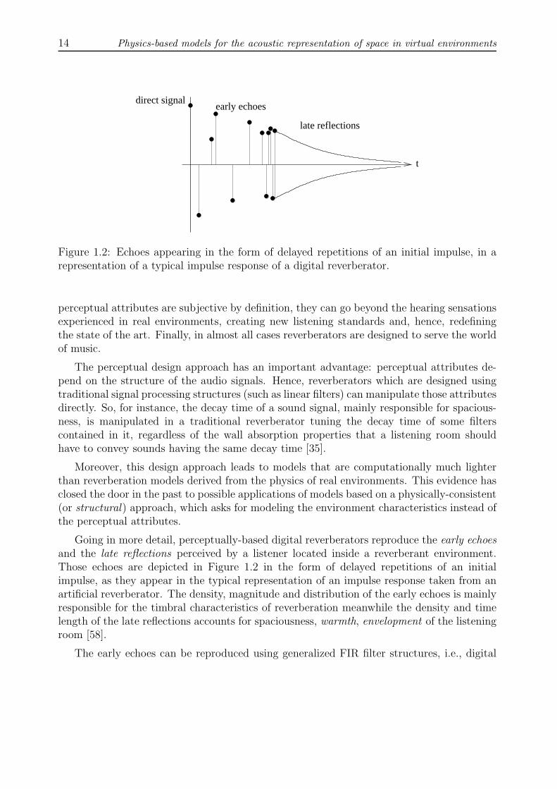
Figure 1.2: Echoes appearing in the form of delayed repetitions of an initial impulse, in arepresentation of a typical impulse response of a digital reverberator.
perceptual attributes are subjective by definition, they can go beyond the hearing sensationsexperienced in real environments, creating new listening standards and, hence, redefiningthe state of the art. Finally, in almost all cases reverberators are designed to serve the worldof music.
The perceptual design approach has an important advantage: perceptual attributes de-pend on the structure of the audio signals. Hence, reverberators which are designed usingtraditional signal processing structures (such as linear filters) can manipulate those attributesdirectly. So, for instance, the decay time of a sound signal, mainly responsible for spacious-ness, is manipulated in a traditional reverberator tuning the decay time of some filterscontained in it, regardless of the wall absorption properties that a listening room shouldhave to convey sounds having the same decay time [35].
Moreover, this design approach leads to models that are computationally much lighterthan reverberation models derived from the physics of real environments. This evidence hasclosed the door in the past to possible applications of models based on a physically-consistent(or structural) approach, which asks for modeling the environment characteristics instead ofthe perceptual attributes.
Going in more detail, perceptually-based digital reverberators reproduce the early echoesand the late reflections perceived by a listener located inside a reverberant environment.Those echoes are depicted in Figure 1.2 in the form of delayed repetitions of an initialimpulse, as they appear in the typical representation of an impulse response taken from anartificial reverberator. The density, magnitude and distribution of the early echoes is mainlyresponsible for the timbral characteristics of reverberation meanwhile the density and timelength of the late reflections accounts for spaciousness, warmth, envelopment of the listeningroom [58].
The early echoes can be reproduced using generalized FIR filter structures, i.e., digital

Chapter 1. Physics-Based Spatialization 15
filters having transfer functions in the following form:
H(z) =M∑i=1
biz−ki , (1.1)
H, in this case, reproducing M echoes of amplitude b1, . . . , bM delayed by k1T, . . . , kMTseconds after the direct signal, respectively (T is the sampling interval in the system).
On the other hand, late reflections are basically reproduced using filter networks capableof providing “dense” responses both in time and frequency [140, 58].
Some interesting considerations can be also done for the user interfaces that can befound on board of artificial reverberators. Traditionally, those interfaces allow to choose thedesired spatial effect through the selection of a mix of physical and perceptual attributes.For example, the user can choose among effects such as “large room” or “dry concert hall”.Nevertheless, the future of these interfaces seems to be oriented toward a more intensive useof the perceptual parameters [78], further increasing the gap existing between the structuraland perceptual design of artificial reverberators for musical purposes.
1.2.3 Physically-oriented approach to reverberation
The exponential nature of the physical problem that, starting from the description of athree-dimensional environment provided with acoustically reflective walls and objects, asksfor finding out the set of echoes that reach a particular point in that environment after ithas been excited by a sound source somewhere located, devises solutions whose computationexplodes as soon as we try to calculate the positions and amplitudes of reflections that followthe early echoes. Models nevertheless exist that calculate that set of echoes with the desiredaccuracy.
Precise computations of the values taken in the spatial domain by the acoustic pressurefunction can be obtained using boundary elements and finite elements methods. These meth-ods compute the three-dimensional pressure field in the discrete space and time [91], startingfrom its differential formulation along with boundary and initial conditions. Although theiraccuracy in solving the difference problem is considered far beyond the precision required insound synthesis, nevertheless unsurpassed results have been obtained using finite elements inthe audio-video simulation of auditory scenes describing dynamic ecological events involvingthe motion of solid objects [109].
The same problem is solved also by finite difference methods. Although less flexible inthe formulation of the difference problem compared with boundary and finite elements, finitedifferences result in simplified numerical schemes that calculate the pressure function over adesired set of spatial locations [18].
So far, the methods which received particular attention by researchers in audio had toprovide solutions suitable for the real time. In particular, ray-tracing [85] and image [5]methods are appreciated for their simplicity and scalability in modeling wave reflection. Infact, following alternative geometrical approaches, both of them allow to calculate the echoes

16 Physics-based models for the acoustic representation of space in virtual environments
that follow the direct signal: the number of reflections that affect an echo, during its journeyfrom the source to the listening point, determines the complexity needed for the computationof that echo. Hence, both methods devise algorithms that provide solutions, whose accuracyin the description of the echoic part of the signal can be tuned proportionally to the availablecomputational resources.
More recently, the importance of modeling diffracted acoustic waves has been demon-strated particularly in propagation domains where the sound source is occluded to the lis-tening point. Studies on wave diffraction yielded efficient modeling strategies based on ageometrical approximation of the diffraction effect [155].
An alternative approach to modeling sound propagation resides in the so called wavemethods. Those methods are based on the linear decomposition of a physical signal into acouple of wave signals, this being possible for several domain fields including pressure fields.Wave signals are then manipulated once the transmission and reflection properties of thepropagation domain are locally known.
Those local properties are transferred into particular elements defined by such methods:Wave Digital Elements in the case of Wave Digital Networks [47, 133, 112], Scattering Junc-tions in the case of Digital Waveguide Networks (DWN) [147], Transmission Line Matrices(TLM) in the case of TLM methods [30]. Such elements receive, process and finally de-liver wave signals in such a way that the global network of elements can be computed by anumerical scheme.
Different wave methods have many points in common. Fundamental relationships existingbetween Wave Digital Networks and DWN have been shown by Bilbao [13]. More in general,there are several basic relationships between wave and finite difference methods [13] andbetween finite differences and finite elements [116]. Although a unified vision of the numericalmethods existing for the simulation of wave fields is far from being proposed, neverthelessmore research should be done to figure out possible links existing among those methods, andto define a common framework where the performance and the computational complexity ofeach method can be compared.
In this work, we will design resonating and sound propagation environments using theWaveguide Mesh, a numerical scheme belonging to the family of DWN. Relationships withfinite differences have been shown for many Waveguide Mesh realizations [158, 50, 13]. InChapter 2 we will address several known properties of the Waveguide Mesh, along with somenovel observations about the numerical behavior of those schemes that may turn to be usefulduring the simulation of wave propagation domains.
1.2.4 Structurally-based artificial reverberators
The design of a structural model, i.e., a model which is capable of synthesizing objectivespatialization cues starting from a set of physical parameters of the auditory scene, has alsobeen considered by researchers. In the past such a model had no chances to be implementedon a real-time application, and even today the resources that are generally needed to achieve

Chapter 1. Physics-Based Spatialization 17
the real time do not justify the realization of a structurally-based artificial reverberator.
If we derive (1.1) from the early response of a real listening environment [17, 121], thenour application will follow an hybrid approach, i.e., structural for the early echoes, andperceptual for the late reflections [140]. The corresponding model, thus, defines a consistentrelationship between the early echoes and the structure of a listening room [58].
In the case when the listening conditions vary in time, for instance in presence of changesin the position of the listening point, geometrical algorithms (such as ray tracing or imagemethods, introduced in § 1.2.3) can be used to compute runtime, without excessive com-plexity, the digital delays and amplitude coefficients contained in (1.1). This enables toreproduce some dynamic spatial cues, such as the ones evoked when the sound source getsoccluded in consequence of changes occurring in the scene description [93].
In parallel with a physically-consistent simulation of the early echoes, efforts have beenmade to match the late reflections with the room characteristics. This should make the audiomore veridical especially in complex VR scenes, where the source and listener positions can bechanged dynamically: for instance, when the listener moves toward a more “open” locationin the auditory scene. Since the real-time constraint suggests to adopt computationally lightmodels, then special maps are needed which establish efficient relationships between theenvironmental parameters and the driving coefficients of the filter networks accounting forthe late reflections.
Those maps must be layered in between the model and the interface. In this way the latereverberation is informed with a scene description. Clearly, such maps can be implementedonce the relationships existing between late reflections and room characteristics are known.If those relationships derive from perceptual considerations, then the resulting reverberatoronce again represents a compromise between the perceptual and structural approach.
In any case such a “layered” approach leads to indirect communication between the re-verberator and its interface. In spite of this, the most recent models for late reverberation (inparticular those employing Feedback Delay Networks) translate into structures whose directaccessibility to certain control parameters envisions closer relationships with the physicalworld [79, 122].
1.3 Physics-based spatialization models
In this section we can outline in more detail the main scope of this work. We willcall physics-based spatialization model a model capable of reproducing objective spatial cues(such as those defined in § 1.1.5) through the simulation of a listening environment whosephysical/geometrical parameters are explicitly represented in the model.
Explicit parameter representation turns out to be a fundamental feature in our model.By means of this property we can keep those parameters simultaneously available at theinterface level, as control parameters, and at the processing level, as driving parameters,with no intermediate stages connecting those two levels.

18 Physics-based models for the acoustic representation of space in virtual environments
map
signal processing signal processing
map
anechoic sound spatialized soundanechoic sound spatialized sound
interface level perceptual values
psychophysical scalesPHYSICS−BASED MODEL
processing level
PERCEPTUAL MODEL
model parametersmodel parameters
scene description
Figure 1.3: Perceptual vs. physics-based approach.
Numerical methods, such as those seen in § 1.2.3, are possible starting points for thedevelopment of physics-based spatialization models. In fact, by means of those methods wecan design models in which:
1. signals are processed through elements, whose driving parameters are directly derivedby the model;
2. the description of the listening environment is directly derived by the model as well.
In Chapter 2 we will see that Waveguide Meshes exhibit both properties, so that theyare eligible for the design of physics-based models.
1.3.1 Physically-informed auditory scales
For what has been said in Section 1.3, a physics-based model looks attractive becauseof the direct representation of a listening environment existing inside it. Figure 1.3 givesa graphical explanation of the differences and relationships existing between the perceptualand physics-based approach.
The weak points, which cannot be addressed by the physics-based approach, reside inthe aforementioned gap existing between physical acoustic measurements and perceptualauditory scales, along with the computational requirements needed by physics-based models.
Concerned with the former point, we propose to evaluate physics-based models perceptu-ally, hence obtaining, using those models, psychophysical scales that are functions of physicalspatial parameters. This sounds quite obvious for certain scales: for example, loudness andpitch are functions of the sound pressure and frequency. On the other hand, the samefunctions become less obvious for other auditory spatial scales such as presence, warmth,

Chapter 1. Physics-Based Spatialization 19
heaviness and so on, for which only relationships with certain properties of the signal havebeen proposed instead, avoiding detailed physical interpretations of those scales [166, 78].
Although the definition of a physics-based psychoacoustics of spatial hearing is far beyondthe scope of this work, nevertheless we will give examples in Chapters 3 and 4 showing that,due to their versatility and accuracy, physics-based models are becoming promising tools forthe simulation of auditory scenes, at least for VR applications, and at most for psychophysicaltesting based on virtual listening environments.
Concerned with the latter point, we hypothesize that humans’ auditory perception of alistening environment translates into simplifications in the models. Although we cannotprove that hypothesis, the experiment carried out in Chapter 4 suggests that physics-basedmodels in practice are not required to simulate all aspects of the listening environment, butthose which are significant for its auditory representation.
This idea of representing the auditory scene instead of the listening environment in totoenvisages new horizons for physics-based spatialization, that remain still widely unexploredalso by this work. Such environments will be captured by “spatial contexts” that, althoughincluding a reduced (however rearranged) set of physical and geometrical figures of theenvironment, nevertheless provide all the psychophysical dimensions needed to convey anexhaustive auditory scene description to a listener.
This kind of approach is already familiar to researchers working with physically-informedmodels for the synthesis of ecological sounds [165, 62]: those models use to capture only somemacroscopic aspects of the physical process that generates a sound, whereas neglect or treatin some simple way more subtle factors acting during the process [34, 125, 118]. Experimentsconducted using physically-informed models have demonstrated that, if correctly conceived,such models capture the most relevant perceptual aspects of the process, meanwhile they(probably) miss other aspects that don’t produce strong auditory cues. Those models canbe used to specify perceptual scales that are functions of the physical parameters, henceinforming about “how do we hear in the world” [61].
Similarly, if successful a physics-based approach to spatialization would be able to explainauditory spatial impressions such as envelopment, warmth and so on by relating them tophysical descriptions of the scene. Psychophysical auditory scales would come out fromsubjective judgments on sounds spatialized by physics-based models containing a precisedescription of the auditory scene.
This intuition is graphically highlighted by the dashed lines depicted in Figure 1.3. Whileenvisioning that scenario, this work only investigates perceptual scales having a clear anddirect physical characterization: distance, that is the argument of Chapter 4, along withroundness and squareness, subjects of Chapter 3.

20 Physics-based models for the acoustic representation of space in virtual environments

Chapter 2
The Waveguide Mesh: TheoreticalAspects
“Per qualche motivo, la violazione della logica mi tocca sul piano morale.”[Carlo Ginzburg. Intervista televisiva sul libro
Il giudice e lo storico. Considerazioni in margine al processo Sofri. 2001.]
“For one reason or another, the violation of logic touches me on the moral side.”[Carlo Ginzburg. Television interview on the book
Il giudice e lo storico. Considerazioni in margine al processo Sofri. 2001.]
As introduced in Section 1.3, the Waveguide Mesh [158] (from here called WM) canbe used as a tool for the synthesis of physics-based models. This fact will be issued moreprecisely in this chapter, along with the theoretical limits that this approach to sound spa-tialization actually exhibits.
Ideal wave pressure fields are mathematically described by a differential equation definedover a problem domain. Solutions for this equation can be investigated after consistent initialand boundary conditions are set, in this way completing the formulation of the differentialproblem. For certain simple boundary conditions, closed-form solutions can be found [102].
Once the problem is addressed in that way, pressure fields take the form of a compositionof waves that propagate along the problem domain. The wave decomposition of a multi-dimensional pressure function that solves the differential problem is a general result, in away that we can study the evolution in time of a pressure function once we know the initialvalues assumed by its wave components and the physical laws that govern the evolution ofthose waves.
WMs, indeed, work in the way just described: by embedding elements that model wavescattering and wave reflection, they process signals that play the role of “wave” signals inthe discrete time and space. In this way, WMs provide a numerical approximation of thepressure waves that propagate along a problem domain. As a direct consequence of thismodeling approach, an approximation of the pressure function can be immediately figuredout by the WM at any processing step.
21

22 Physics-based models for the acoustic representation of space in virtual environments
An incorporation of the WM in the framework of DWN [147] has been recently made byBilbao [13]. DWN allow to model several propagation fields, whose differential equations canbe numerically computed using wave scattering methods. Many differential problems thatcan be dealt with using DWN have practical application in acoustics and sound synthesis.
DWN have close connections with the so-called Finite Difference Time Domain methods,so that several properties holding for the latter family can be exported to the former one.In particular, WMs have a direct correspondence with Finite Difference Schemes [157]: thisanalogy enables to assess with precision, by means of a Von Neumann analysis [152], theerror introduced by the WM in the approximation of the exact solution of the differentialproblem. The Von Neumann analysis can be extended to the various formulations [138,13] and geometries [160, 50, 24] of the WM, and informs about the accuracy provided bysimulations that are made using the WM.
The reader interested in a deeper comprehension of the WM, in its several formulations,is encouraged to refer to Bilbao [13, 14], where a rigorous formal definition of the WM in theframework of DWN is proposed, along with its numerical properties and relationships withFinite Difference Schemes.
Most of the analyses presented in the literature, evaluating the error introduced by anumerical scheme, do not deal with the spectral distortions that affect the output as aconsequence of this error. As a rule of thumb, it is assumed in literature that numericalmethods provide results whose accuracy decays with increasing frequency or, in other words,that such results are unreliable in the high frequency.
This is certainly true, due to the unavoidable finite precision of the model, along with thediscrete (bandlimited) representation of the physical signals that are involved in the process.On the other hand, this lack of results sometimes puts the model designer in trouble whenshe must determine the granularity of the domain description, in order to obtain a certainaccuracy in the simulations up to a specific frequency.
Another issue which is often neglected by numerical analysis is how to choose the temporalgranularity of the simulations. That issue is usually a minor problem in most applications,since numerical schemes are typically worked out offline, in a way that oversampling themin time is not so critical in the majority of cases.
In the audio field, the real time is a major concern. This concern is even more compellingas long as spatialization is taken into account (refer to § 1.2.2). Hence, a precise knowledgeof the consequences which follow by choosing a particular time step for a scheme is certainlyinformative for the designer of audio systems. First of all, it would give information aboutthe spectral characteristics of the output signals. More in general, the timing effects shouldbe under control when a real-time execution of a numerical simulation is planned on signalprocessors, or other types of architectures, that are capable of processing signals at a fixedsampling rate: in that case, the time step becomes a constraint in the problem, in a waythat its effects must be clear to the designer since the beginning of the design activity.
We have conducted this kind of analysis for the WM. For sake of simplicity the analysishas been limited to WM geometries that model two-dimensional (2-D) problem domains,

Chapter 2. The Waveguide Mesh: Theoretical Aspects 23
namely the square, the triangular and the hexagonal WM. Although, obviously, 2-D domainscannot account for three-dimensional (3-D) pressure fields, nevertheless the proposed analysiscan be straightforwardly extended to the third dimension. Moreover, some conclusions thathave been demonstrated in the 2-D case hold also for the 3-D case: first of all, that WMgrids containing gaps in between are proportionally less efficient than gap-free grids.
We complement the analysis presenting a curious interpretation of the square WM, thatmotivates from a physical viewpoint the peculiar symmetry exhibited by its frequency re-sponse, along with a method that, exploiting this symmetry, halves the number of compu-tations that are required to calculate that response.
An important question concerning the designer of spatialization tools is how to control, ina WM, wave transmission and wave reflection for a particular problem domain. Once again,the waveguide approach yields a direct way to deal with those aspects of the problem. In fact,WMs allow a local selection of the impedance, by means of which the acoustic properties ofmaterials can be completely specified. In this way the problem domain can be characterized.A thorough treatment on how to set impedances in the WM has been made by Bilbao [13].
Rather, in this work we focus on boundary reflections. In particular, we have studied howaccurately they can be modeled using scattering. We have found evidence that boundaryscattering models are more accurate, since their impedances account for the direction ofthe incident wave, and waves are reflected along directions that are consistent with theimpedance value. Again, the analysis has been limited to 2-D propagation domains, althoughits conclusions may be qualitatively extended to the 3-D case, and quantitatively assessedvia WM simulations of 3-D bounded propagation domains.
Finally, we propose a modified version of the WM that exhibits a high accuracy. A wayfor reducing the numerical error introduced by the WM has been investigated by severalresearchers involved in the subject, and finally a technique to manipulate this error has beenproposed along with an offline method that performs that manipulation [137]. Nevertheless,a numerical scheme that realized that manipulation online had not been presented so far.Here we propose a method enabling online manipulation, then we construct a modified WMwhere the numerical error has been minimized.
This chapter embraces all the subjects just outlined. It is structured in the followingway:
• a minimum set of basic concepts, necessary to understand the WM in its several for-mulations, is introduced;
• a spatial and temporal frequency analysis of the square, triangular and hexagonal WMis conducted. By means of that analysis the spectral properties of the responses comingout from those meshes are motivated;
• the previous analysis is complemented with further observations on the response of thesquare WM, and a technique for computing that response that halves the number ofcomputations is proposed;

24 Physics-based models for the acoustic representation of space in virtual environments
• a strategy to improve the accuracy in the simulation of the boundary is given;
• a numerical scheme which minimizes the numerical error is proposed, along with atechnique to compute it.
2.1 Basic concepts
Here, we introduce some basic concepts of wave propagation in pressure and mechanicfields, together with their modeling using the WM.
2.1.1 Wave transmission and reflection in pressure fields and uni-form plates
In a pressure field, the wave equation that expresses a deviation p from atmosphericpressure over a coordinate point (x, y, z) is written at time t as
1
c2
∂2p
∂t2=∂2p
∂x2+∂2p
∂y2+∂2p
∂z2. (2.1)
This equation describes the case, considered representative enough for real situations, oflinear pressure fields. The parameter c gives the speed at which pressure waves propagatealong the field domain [102]. Linear pressure fields describe lossless, constant-impedance andconstant-speed wave transmission domains.
A straightforward particularization of this equation to 2-D domains (that is, letting forexample ∂2p/∂z2 ≡ 0) leads to a description of only a reduced set of 2-D wave propagationproblems. In fact such problems (mainly referring to mechanical and electro-magnetic fields)are described by a more general partial linear differential equation system, that defines theParallel-Plate Transmission Line problem. The parallel-plate transmission line problem,in particular, can account for local variations of the medium parameters (represented bycapacitance and inductance), that induce corresponding variations in the impedance andloss characteristics of the problem domain, and in the wave propagation speed [13].
For our purposes, the case of constant capacitance and inductance is sufficient. Asexplained, this corresponds to analyzing equation
1
c2
∂2p
∂t2=∂2p
∂x2+∂2p
∂y2, (2.2)
that is clearly a reduced version of (2.1) to the 2-D case. This means that we will limit our 2-Dcase studies to problems which are described by (2.2). This restriction must not be consideredas a limitation in this work, whose main scope is the modeling of 3-D linear pressure fields.In this perspective, the description of wave propagation problems via Equation (2.2) isparticularly attractive, since it translates into a major simplification of the corresponding

Chapter 2. The Waveguide Mesh: Theoretical Aspects 25
WMs compared to those modeling 3-D domains, without loss of generality of most of theconclusions coming out by modeling (2.2) instead of (2.1).
The presence of a boundary induces the phenomenon of wave reflection. We focus onthe reflection of sound waves, giving some basic physical laws whose validity holds in thecase of locally reacting surfaces, i.e., surfaces whose reaction to incident waves is pointwise,independently of the motion of neighboring surface points [90].
The impedance z is defined as the ratio between pressure and normal fluid velocity, v(n):
z =p
v(n). (2.3)
In our case of interest, the surface reflects an incident pressure wave, pi, in a way that eachfrequency component of the reflected wave, pr, is both changed in amplitude and phase.Hence, reflection can be conveniently expressed in the frequency domain in terms of a complexratio (called reflection factor) between the Fourier transforms of the reflected and incidentwave, respectively Pr and Pi:
R(f) =Pr(f)
Pi(f). (2.4)
In the case of real surfaces, reflection factors change to a broad extent, according tothe material the surfaces are made of. Most of those surfaces exhibit a lowpass behaviorwith respect to wave reflection. In other words, they mainly absorb high frequency wavecomponents.
It can be shown that relation
Z
Z0
=1
cos Θ
1 +R
1−R(2.5)
holds between the (Fourier-transformed1) impedance Z of a surface point and its reflectionfactor. In (2.5), Z0 = ρ0c is the acoustic impedance of the transmissive medium (ρ0 is thedensity of air), and Θ is the angle of incidence. Figure 2.1 explains wave reflection graphicallyin the case when the incident wave is reflected out from the surface along a single direction,forming with the normal an angle which is equal to the angle of incidence. This kind ofreflection commonly takes place in optical mirrors.
2.1.2 WM models
Let us sample a P -dimensional domain into equal elements (for instance, volume elementsin the case of a 3-D pressure field) having N facets, each one of those being centered around aposition J = (x1, . . . , xP ); let us model any of those elements as a N-port scattering junction[147] in a way that, at any time step, each element receives and scatters out one-dimensionalwaves through its N facets:
p+i (J , nT ) , p−i (J , nT ) , i = 1, . . . , N , (2.6)
1in most of the literature the impedance is directly defined in the frequency domain.

26 Physics-based models for the acoustic representation of space in virtual environments
incident wave
reflected wave
Θ
Figure 2.1: Wave reflection.
respectively. Figure 2.2 reports an example for a pressure field that has been spatiallysampled into cubic elements: for each element, six pairs of input and output pressure wavesmove instantaneously in and out, respectively to and from the element. In that figure onlytwo elements have been reported, along with their (two) mutual incoming/scattered waves.
Kirchoff’s laws (namely, conservation of the instantaneous power) yield an instantaneousrelation between the scattered and the incoming waves. The constancy of the mediumcharacteristics among adjacent elements provides lossless transmission at a constant speed(i.e., adaptation between adjacent junctions), in a way that this relation simplifies to
p−i (J , nT ) =2
N
N∑k=1
p+k (J , nT )− p+
i (J , nT ) , i = 1, . . . , N , (2.7)
in which, without loss of generality, we consider pressure waves.The WM model states that scattered waves take exactly one time step to reach an
adjacent scattering junction. This makes the resulting scheme explicitly computable. Infact, referring once again to Figure 2.2, we have that two adjacent scattering elements facingeach other through facets indexed r and l, respectively located at discrete-space coordinatesJ and J +Dur, define the following relations:
p+r (J , nT + T ) = p−l (J +Dur, nT ) (2.8a)
p+l (J +Dur, nT + T ) = p−r (J , nT ) (2.8b)
where the spatial step D separates adjacent elements along the direction defined by ur, andthe temporal step T separates subsequent discrete-time evolutions of the scheme.
From Equations (2.8a) and (2.8b) we observe that each scattering element obtains thevalues of its incoming waves from values previously scattered by adjacent elements. Thosevalues are then used to compute new scattered waves at the current time step, via a simplecomputation such as (2.7). This scheme, hence, is inherently well-suited for implementation

Chapter 2. The Waveguide Mesh: Theoretical Aspects 27
p l+(x+D,y,z,nT+T)
p r+(x,y,z,nT+T) p l
−(x+D,y,z,nT)
J u+D rlr
p r−(x,y,z,nT)
J
Figure 2.2: Two adjacent six-facets elements forming a 3-D spatial domain. Those elementsare centered around positions J = (x, y, z) and J + Dur = (x + D, y, z), respectively, andthey have been modeled as scattering junctions. At time step nT output pressure waves, p−land p−r , are scattered out from facets l and r: they respectively become incoming pressurewaves, p+
r and p+l , for the opposite element at time step nT + T .
on parallel architectures. Although its implementation at audio sample rates on a currentsignal processing device, such as a DSP, limits the complexity of the scheme to few scatteringjunctions, on the other hand this complexity can be raised up to virtually no limits as soonas the scheme is embedded on some kind of modular architecture capable of providing,individually for each element, shifts as those described by Equations (2.8a) and (2.8b), andsignal processing such as that seen in (2.7).
2.1.3 Digital Waveguide Filters
So far, we have seen a method that computes wave propagation along unbounded, idealmedia as described by (2.1). We now outline the Digital Waveguide Filter (briefly, DWF),a block that models waveguide terminations and, for this reason, can be used to bound aWM [159]. Later in this chapter we will see how we use DWFs to model the boundary of apropagation domain.
Equation (2.4) suggests that, in a WM, the reflection factor can be modeled by a dig-ital filter, whose transfer function calculated between incoming and outgoing wave signalsresembles R up to a certain frequency (at most the Nyquist frequency). We will label thisdiscrete-time transfer function with the same symbol, deliberately confounding the reflectionfactor with its realization, in the discrete-time, obtained using a DWF. More precisely, thez-transform of this filter can be put in the following form [98]:
R(z) =b0 + b1z
−1 + . . .+ bMz−M
1 + a1z−1 + . . .+ aP z−P. (2.9)

28 Physics-based models for the acoustic representation of space in virtual environments
Z r Z 2
Z 3
Figure 2.3: Particular of a representation of a waveguide network. Three waveguides, eachone having its own impedance, and three scattering junctions can be seen. One waveguideterminates against a reflective surface having impedance Zr.
In the case when we are modeling, instead of a multi-dimensional pressure field, a networkof waveguides each one having its own impedance, Equation (2.7) can be generalized toaccount for those individual impedances. In fact, considering N ideally joint waveguideshaving impedances respectively equal to z1, . . . zN , then Kirchoff’s laws yield a formula thatputs scattered waves in relation with incoming waves in the transformed domain [147]:
P−i =
2N∑k=1
P+k /Zk
N∑k=1
1/Zk
− P+i , i = 1, . . . , N . (2.10)
Figure 2.3 illustrates a particular in a representation of a waveguide network, where ajunction leading to a reflective surface has been modeled to have an impedance equal to thesurface impedance Zr. Such a network can represent, for instance, a network of ideal pipesor a cable network. A WM is one particular realization of a waveguide network, made ofdigital waveguides having all the same impedance and unitary length.
Equation (2.10) allows to model junctions, in the WM, accounting for the boundaries interms of their reflection factor. In fact (refer to Figure 2.3) it is sufficient to consider such“boundary junctions” as connecting one or more waveguides which are lumped in a mediumhaving its own impedance, where waves cannot propagate. In that case Equation (2.5) canbe substituted inside (2.10), in a way that the reflection factor takes part in the scatteringprocess. To obtain this, we impose that boundaries neither accept nor reflect back wavesto the junction (i.e., that signals both coming from and scattered to waveguides which arelumped in the boundary are null).
In the case of a 2-port scattering junction modeling the termination of an ideal one-dimensional air duct having impedance Z0, (2.10) yields
P− =Zr − Z0
Zr + Z0
P+ , (2.11)

Chapter 2. The Waveguide Mesh: Theoretical Aspects 29
where Zr is the impedance at the termination. Hence, the reflection factor of the terminationis equal to
R =P−
P+=Zr − Z0
Zr + Z0
. (2.12)
If we explicit the impedances as function of the reflection factor in (2.12), we have
ZrZ0
=1 +R
1−R, (2.13)
that equals (2.5) in this particular case, in which we have assumed Θ = 0.
2.2 Spatial and temporal frequency analysis of WMs
The original question, leading to the analysis presented in this section, is the followingone: let us simulate a WM model at a temporal step T . Where is the highest representativefrequency component contained in the responses coming out from that simulation?
The Nyquist frequency, which is equal to half of the sampling frequency Fs:
Fs2
=1
2T, (2.14)
although being an absolute (and obvious) upper limit for the responses coming out fromthe model, does not give a general answer to that question. In fact, such responses havedifferent upper frequency limits according to the mesh geometry. To demonstrate this, wemust understand how the spatial traveling wave components are simulated by the model.
2.2.1 Temporal frequencies by spatial traveling wave components
The way of partitioning the propagation domain into scattering elements can be chosenbetween several geometries (for example, Figure 2.2 depicts a cubic geometry). As a con-straint in this choice, we will limit to partitions where all scattering elements have the sameextension (say, volume in the 3-D case). In practice, we will only deal with WMs whereadjacent scattering junctions are separated by a common spatial step, D.
Each choice results in a different tessellation of the spatial domain. Figure 2.4 showssome possible geometries of the WM, both 2-D and 3-D.
Equation (2.7) shows that the pressure over a scattering element is completely describedby the total incoming wave pressure. In fact, it can be seen that this sum gives the actualpressure value pJ associated to that element [158], that is, rearranging (2.7):
pJ(J , nT ) = p+i (J , nT ) + p−i (J , nT ) =
2
N
N∑k=1
p+k (J , nT ) for each i . (2.15)
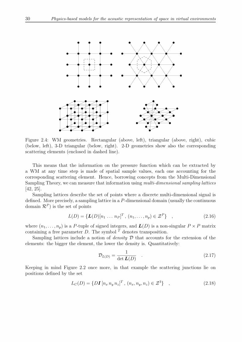
30 Physics-based models for the acoustic representation of space in virtual environments
Figure 2.4: WM geometries. Rectangular (above, left), triangular (above, right), cubic(below, left), 3-D triangular (below, right). 2-D geometries show also the correspondingscattering elements (enclosed in dashed line).
This means that the information on the pressure function which can be extracted bya WM at any time step is made of spatial sample values, each one accounting for thecorresponding scattering element. Hence, borrowing concepts from the Multi-DimensionalSampling Theory, we can measure that information using multi-dimensional sampling lattices[42, 25].
Sampling lattices describe the set of points where a discrete multi-dimensional signal isdefined. More precisely, a sampling lattice in a P -dimensional domain (usually the continuousdomain RP ) is the set of points
L(D) = L(D)[n1 . . . nP ]T , (n1, . . . , np) ∈ ZP , (2.16)
where (n1, . . . , np) is a P -tuple of signed integers, and L(D) is a non-singular P × P matrixcontaining a free parameter D. The symbol T denotes transposition.
Sampling lattices include a notion of density D that accounts for the extension of theelements: the bigger the element, the lower the density is. Quantitatively:
DL(D) =1
detL(D). (2.17)
Keeping in mind Figure 2.2 once more, in that example the scattering junctions lie onpositions defined by the set
LC(D) = DI [nx ny nz]T , (nx, ny, nz) ∈ Z3 , (2.18)

Chapter 2. The Waveguide Mesh: Theoretical Aspects 31
where I is the 3 × 3 identity matrix and D is the spatial step chosen for that WM model.In particular, it is DLC(D) = 1/D3.
The Multi-Dimensional Sampling Theorem specifies the (P -dimensional) support, L∗(D),containing the frequency components ξ of a signal defined over L(D). In this way, we canprecisely assess the spectral information provided by the discrete-space function defined bythe WM at any time step. For example, in the case of the 3-D rectangular WM the spatialfrequencies of the discrete pressure function pJ(J , nT ) , J ∈ LC(D), observe at any timestep the following condition on the support:
ξ = |ξx ξy ξz|T : |ξx| <1
2D, |ξy| <
1
2D, |ξz| <
1
2D. (2.19)
such that L∗C(D) is a cube of volume 1/D3 centered around the spatial frequencies origin.The speed of propagation of a numerical wave component traveling along a WM is a
function of its own spatial frequency. We express this calling c(ξ) this propagation speed,when traveling wave components have spatial frequency equal to ξ. The dependency ofthe propagation speed on spatial frequency is part of the numerical error introduced bythe model: in fact, contrarily to that, Equation (2.1) envisages a common speed for anycomponent.
This error is known in literature as dispersion and, as mentioned in the beginning of thischapter, can be precisely calculated by conducting a Von Neumann analysis on the scheme[152]. As a direct consequence, the Von Neumann analysis highlights about the value of c(ξ)for any WM geometry. On the other side, by conducting a stability analysis, condition
c(ξ) ≤ 1√PDFs (2.20)
is found to hold for the propagation speed in a WM modeling a P -dimensional propagationdomain [152].
Once c(ξ) is known over L∗(D), we can finally answer the initial question. In fact,spatial frequencies ξ are turned into corresponding temporal frequencies f by multiplyingthe propagation speed times the spatial frequency magnitude:
f = c(ξ)
√ξTξ , (2.21)
so that the upmost frequency contained in the response of a WM is equal to
f (max) = maxξ∈L∗(D)
c(ξ)
√ξTξ , (2.22)
where the maximum is calculated over the support where the spatial frequencies are defined.Following with the example of the 3-D rectangular WM, in that case the Von Neumann
analysis states that the shortest spatial wave components also travel at the highest propa-gation speed. Thus, by (2.22) we obtain immediately
f(max)C =
1√3DFs
√(1
2D
)2
+
(1
2D
)2
+
(1
2D
)2
=Fs2
. (2.23)

32 Physics-based models for the acoustic representation of space in virtual environments
Hence, that particular WM geometry produces responses whose spectral information matchesthe Nyquist value.
Starting from this overview on the frequency analysis of the WM, and its exemplificationto the 3-D rectangular geometry, the reader is referred to Paper C for a comprehensivetreatment of the 2-D triangular topology. In that work the hexagonal geometry is issuedas well, as an example of a domain partition where the scattering elements have the samevolume but different orientations.
From that treatment, two main conclusions are reported here:
1. compared with the rectangular geometry, the triangular WM processes more effi-ciently signals whose spatial frequency support is symmetrical around the origin ofthe frequency axes. Such signals are created, for example, by excitations having omni-directional directivity;
2. WMs containing gaps in their grids of scattering junctions (such as, for example, thehexagonal WM) produce responses that are proportionally less informative comparedto those coming from gap-free mesh grids.
These two considerations can be qualitatively generalized to both 2-D and 3-D WMs. Quan-titative figures can be calculated for the geometries that have not been explicitly consideredin this work, by repeating the spatial frequency analysis starting from the related samplinglattice, and from the results provided by the corresponding Von Neumann analysis.
2.2.2 The frequency response of rectangular geometries
Equation (2.23) proves that 3-D rectangular WMs respond up to the Nyquist frequency.Repeating the calculation for the 2-D case is even easier. Nevertheless, rectangular geome-tries are characterized by responses that mirror at half of the Nyquist frequency.
This characteristic can be motivated reconducting the z-transform of those responses toa peculiar numerical property of the scheme [158]. Equivalently, it can be explained in theuntransformed domain provided that the discrete-time pressure function defined on L(D)observes the following two properties:
pJ(J , 2nT ) = 0 , J ∈ L1(D) (2.24a)
pJ(J , 2nT + T ) = 0 , J ∈ L(D) \ L1(D) (2.24b)
in which the sampling lattice L1(D) is a subset of L(D), having density DL1(D) equal to halfthe density of L(D). Properties (2.24a) and (2.24b) imply that any response, which is takenin correspondence of a scattering junction, presents sample values that are interleaved, intime, with null values. This results in mirroring at half Nyquist in the temporal frequencydomain.
Rectangular geometries exhibit this characteristic as soon as an initial excitation is formedby setting the scattering junctions with initial pressure values, pJ(J , 0), that respect property

Chapter 2. The Waveguide Mesh: Theoretical Aspects 33
(2.24a): in this way, any scattering element in L1(D) delivers null wave signals. At time stepT those signals reach the adjacent elements, which belong to L(D) \L1(D). Those elementshave just delivered (in general) non-null signals at time step 0 and are receiving null signalsat time step T , hence their pressure values become null in their turn. In this way at timet = T the roles of the junctions belonging to L1(D) and L(D)\L1(D) are exchanged. Clearly,this kind of swapping goes on indefinitely, in a way that a signal coming out from any pointof the WM contains non-null samples interleaved with null values. Thus, properties (2.24a)and (2.24b) are satisfied.
Since the response of a WM is obtained initializing the system with a function, theimpulse [98], that respects (2.24a) at t = 0, then that response will mirror at half Nyquistwherever we pick it up from the WM.
It is interesting to look for a modified version of the rectangular scheme that producesresponses whose spectral content is limited to half of the Nyquist frequency. In fact we expectthat such a modification, avoiding redundant computations, leads to a more economic wayof computing those responses compared with the original rectangular WM. In practice wemust look for a modified WM scheme that avoids processing the spatially interleaved nullsamples, meanwhile dealing with non-null samples in the same way the original WM does.
The reader is sent to Paper D, where a modified scheme working in the way just out-lined is presented, together with figures that confirm that it requires less (more precisely,half) operations and memory occupation to compute a response. Similar results have beenindependently obtained also by Bilbao, who emphasizes different aspects in those schemes[13, 12].
The sampling lattice described by the modified rectangular WM resembles some samplingschemes used for the discretization of motion pictures. Those schemes efficiently encode themulti-dimensional information by interleaving the image samples both in time and space[25].
2.2.3 WMs as exact models of cable networks
We conclude the spatial and temporal frequency analysis of the WM giving an interestingcharacterization, that confirms that dispersion is introduced as soon as we simulate propa-gation along infinite directions using a model that can account only for a finite number ofdirections.
In § 2.1.3 we have mentioned that WMs are, in fact, numerical models of special net-works of waveguides, in which all waveguides have the same length and impedance. Thosenetworks model, for instance, compositions of air ducts or ideal strings in which each waveg-uide element is ideally joint with other waveguide elements. Also, we have seen that WMscan model multi-dimensional homogeneous propagation domains, to an extent that is quan-titatively assessed by the Von Neumann analysis in terms of dispersion error, and by thefrequency analysis in terms of upper frequency limit of the simulations.
A WM reduces to the Digital Waveguide [149] as soon as we particularize it to the 1-D

34 Physics-based models for the acoustic representation of space in virtual environments
DISPERSION FINITE BANDWIDTH
N−D medium Waveguide network WM
Figure 2.5: Simulation errors produced by the reformulation of multi-dimensional propaga-tion domains into waveguide networks and digital WMs.
case. In that case dispersion disappears, suggesting that that kind of numerical error comesinto play only if we want to model multi-dimensional wave propagation. Then, the questionis: are WMs responsible of dispersion, or, conversely, is dispersion the general consequenceof a waveguide approach to multi-dimensional wave propagation?
The same question has been reformulated in Figure 2.5, where we have also anticipated apossible answer: while dispersion is introduced by the reformulation of the multi-dimensionalpropagation domain into a waveguide network, on the other hand a WM modeling thatnetwork causes the number of traveling wave components to become finite.
If that answer is true, then we can reconduct the differences existing between the responsecoming from an ideal propagation medium, and the response taken from the WM, to twoindependent causes: dispersion artifacts, caused by discretization in the number of directionsof propagation, and finite bandwidth, caused by discretization in space and time.
We will be able to demonstrate this only in the particular case of 2-D rectangular waveg-uide meshes simulating rectangular, ideally bounded domains, such as rectangular mem-branes ideally clamped at the edges. In order to do this we introduce orthogonal cablenetworks, that are orthogonal sets of interconnected cables modeled as ideal strings, simplysupported (i.e., ideally clamped) at the ends. Those networks have been first studied in thefield of applied mechanics. Refer to the 2-D rectangular WM of Figure 2.4 for a graphicdescription of the orthogonal cable network.
Before an exact solution of the cable network problem had been found, curiously thepreferred modeling approach to that problem was the membrane analogy [146]: by means ofit, the (analytical or simulated) solution provided by a physical membrane resembling thecable network according to certain specifications was used to approximate the cable networkproblem solution. That approximation had been found to be as more accurate, as larger thenumber of cables was; in any case, the membrane analogy provided an accurate solution aslong as only the first (low frequency) vibration modes were considered.
Compared to the WM approach, the membrane analogy establishes a “backward link”between homogeneous, omni-directional propagation media and their modeling using waveg-uide networks. In fact, the solution provided by an omni-directional medium is used toapproximate a network where waves can propagate along a finite number of directions.Clearly, the membrane analogy results to be particularly accurate in the simulation of thefirst vibration modes [146], exactly as WMs well approximate an omni-directional mediumin the low frequency [13, 50].

Chapter 2. The Waveguide Mesh: Theoretical Aspects 35
The first exact solution of the cable network problem is dated 1985 [37]. That solutionmakes use of the transfer matrix method : it comes out by first calculating a transfer matrixfor each single section of cable, then composing those matrices to successively obtain thetransfer matrix for a joint, a chain, and finally the entire network.
The equations governing the displacement w in an orthogonal cable network are synthet-ically proposed here, in the case of cable networks having the same pretension, length andmass per unit length along both (x and y) directions. Such equations consist of [27]:
1. one natural vibration equation for each individual (both x- and y-oriented) section (i, j)of cable connecting two joints,
∂2w(i,j)
∂x2+ω2
c2w(i,j) = 0 or
∂2w(i,j)
∂y2+ω2
c2w(i,j) = 0 , (2.25)
where ω = 2πf is the pulsation of a vibration at frequency f , and c is the speed atwhich waves propagate along a cable section;
2. a condition of continuity across each joint, located on position J ,
w(i1,j1)(J) = w(i2,j2)(J) = w(i3,j3)(J) = w(i4,j4)(J) for all joints , (2.26)
where (i1, j1), . . . , (i4, j4) are cable sections connected together in a joint, includingparticular joints located at the cable ends;
3. a condition of equilibrium for all internal nodes,
∂w(i2,j2)
∂x−∂w(i1,j1)
∂x+∂w(i4,j4)
∂y−∂w(i3,j3)
∂y= 0 for all internal nodes , (2.27)
where (i1, j1), . . . , (i4, j4) are cable sections joint together in an internal node, suchthat (i2, j2) follows (i1, j1) along the x-direction and (i4, j4) follows (i3, j3) along they-direction;
4. conditions of simple support at all cable ends.
This problem has been solved in closed form by using a transformation technique known asthe double U-transformation. This technique is powerful enough to yield analytical solutionsalso in the case of beam networks [44, 27] and orthogonal cable networks subjected to movingforces [28] or having periodically distributed supports [26].
In our case of interest, the pulsations of the modes vibrating in a square cable networkmade of N − 1 cables, having length L, are the solutions of the equation [27]
cosπω
Nω0
=1
2
(cos
πr
N+ cos
πs
N
), r, s = 1, . . . , N , (2.28)

36 Physics-based models for the acoustic representation of space in virtual environments
r s f r s f r s f r s f
1 1 0.0625 4 2 0.1925 4 4 0.2500 4 6 0.30751 2 0.0982 1 5 0.2064 5 3 0.2500 6 4 0.30752 1 0.0982 5 1 0.2064 6 2 0.2500 5 5 0.31252 2 0.1250 3 4 0.2194 7 1 0.2500 4 7 0.32641 3 0.1367 4 3 0.2194 2 7 0.2673 7 4 0.32643 1 0.1367 2 5 0.2241 7 2 0.2673 5 6 0.34172 3 0.1583 5 2 0.2241 3 6 0.2759 6 5 0.34173 2 0.1583 1 6 0.2327 6 3 0.2759 5 7 0.36331 4 0.1736 6 1 0.2327 4 5 0.2806 7 5 0.36334 1 0.1736 1 7 0.2500 5 4 0.2806 6 6 0.37503 3 0.1875 2 6 0.2500 3 7 0.2936 6 7 0.40182 4 0.1925 3 5 0.2500 7 3 0.2936 7 6 0.4018
7 7 0.4375
Table 2.1: Positions in frequency of the vibrating modes of a rectangular WM sized 8 × 8with rigid boundary terminations.
as N is the number of sections forming each cable. In that equation it is
ω0 =πc
L. (2.29)
A cable network is a waveguide network. In fact, Equations (2.25) hold for a waveguidewhere waves propagate at speed c along it. Moreover, Equations (2.26) and (2.27) hold inparticular in a series connection of waveguides [13]. Hence, a waveguide network providedwith boundary conditions that simulate a rigid termination equals a simply supported cablenetwork. From that it comes out that a square waveguide network sized L × L, whosewaveguides have a length equal to D in a way that it is L = ND, must vibrate at thepulsations given by Equation (2.28), which can be rewritten as
πω
Nω0
= arccos
[1
2
(cos
πr
N+ cos
πs
N
)]± 2kπ , r, s = 1, . . . , N , k ∈ N . (2.30)
We now move to the discrete time and space, i.e, we change the waveguide network intoa rectangular WM. This corresponds to substituting the waveguides in the network withunit-length Digital Waveguides. Those new elements cannot vibrate but at one frequency,so that their pulsation is unique, i.e., k = 0. Moreover they force waves to travel at speedc = D/T , where T is, as usual, the temporal step of the simulation.
Then, by (2.29) we have
πω
Nω0
=πω
N
ND
πc=ωD
c= ωT = 2πfT = 2π
f
Fs, (2.31)

Chapter 2. The Waveguide Mesh: Theoretical Aspects 37
0 0.1 0.2 0.3 0.4 0.5−20
−10
0
10
20
30
40
50
60
Normalized Frequency
dB
Figure 2.6: Frequency response from a rectangular WM sized 8 × 8. (×): frequency valuesobtained for the same WM using (2.32).
so that we finally obtain the modal frequencies in the WM:
f =Fs2π
arccos
[1
2
(cos
πr
N+ cos
πs
N
)], r, s = 1, . . . , N − 1 , (2.32)
where the cases r = N and s = N have been excluded, since Digital Waveguides made ofN pairs of unit delay elements, rigidly clamped at both ends, cannot vibrate but at N − 1frequencies. By the way, the case r = s = N results in frequencies that are equal to theNyquist frequency (2.14).
As an application example let us consider a rectangular WM sized 8×8, sampled using aunitary temporal step. Equation (2.32) yields 49 modal frequencies, that have been reportedin Table 2.1 in order of increasing frequency, together with the corresponding values r ands. Those values are also compared, in Figure 2.6, with the modal frequencies taken from asimulation of the same WM that has been excited in correspondence of a corner, and whoseresponse has been acquired in correspondence of the opposite corner.
It can be seen that the correspondence between the calculated positions in frequencyof the vibration modes, and the positions of the same modes when they are generatedby a simulation, is excellent. This result is consequence of the analogy existing betweenrectangular WMs and discretized orthogonal cable networks.
It should not be difficult to extend the same analogy to the third dimension. Rather, anextension to non-orthogonal cable networks, aiming at finding analogies for example with 2-D

38 Physics-based models for the acoustic representation of space in virtual environments
FDW
FDW
p 2+
3−PORTLSJ
p 2+
p −2
p 1−
p +1
p −2
p 1−
p +1
Θ
Figure 2.7: Individual processing of two incident wave signals by means of DWF transferfunctions (left). Integrated processing of two incident wave signals by means of boundaryscattering junctions (right).
triangular WM geometries, seems to ask for a good practice with the double U-transform.
2.3 Scattered approach to boundary modeling
As we have introduced in § 2.1.3, the simulation of a reflective and/or absorbing boundaryturns out to be quite straightforward if DWFs are used to terminate the branches in a WM,in correspondence of the domain boundary. In particular, we have seen that boundaryconditions, expressed as a variation in the impedance of the medium along the boundary,can be embedded inside special 2-port scattering nodes, provided that the wave signalscoming back and forth the reflective medium are permanently set to zero in those nodes.
In this section we deal with the issue of boundary modeling in further detail, starting fromthe following question: how can we model multiple reflections simultaneously occurring atthe same point? In other words, what if the boundary junctions include more than one portfacing the domain of propagation? This happens for example in the triangular geometries,both 2-D and 3-D (see Figure 2.4).
The analysis presented in § 2.1.3 is limited to single reflections, i.e., to 2-port scatteringjunctions. As a starting point, that analysis is sufficient to treat multiple reflections indi-vidually in a way that they can be modeled one by one, using 2-port scattering junctions(equivalent to DWFs) independently working one from the other, hence avoiding any kindof communication between wave signals coming from different directions. Figure 2.7 (left)illustrates this situation in the case of two incoming wave signals.
Alternatively, we note that Equation (2.10) accounts in general for N ports. Hence, bythat equation we can immediately extend boundary reflection to N−1 incoming wave signals(Figure 2.7, on the right side, shows this for N = 3).
We have not proved that the “scattered” approach to boundary reflection leads in general

Chapter 2. The Waveguide Mesh: Theoretical Aspects 39
mk
R s
pp
ir
Figure 2.8: 1-st order spring/damper system.
to more accurate simulations. In spite of that, its application to cases where we can comparethe model with the behavior of a physical boundary shows that the scattered approach toboundary modeling, in those cases, models wave reflection more naturally. As a consequenceof that, simulations adopting scattering junctions at the boundary provide more accuratepositioning of the modal frequencies.
In the following of this section we will outline a scattered reflection model. During theexposition we will also review the DWF method for the design of boundaries in the WM[159] having a consistent physical interpretation [90]. The organization of this section tookadvantage also from the work of Fabio Deboni [36].
2.3.1 DWF model of physically-consistent reflective surfaces
The reflection factor R can be measured for many materials, as a function of the frequencyof the incident wave component [90]. Table 2.2 shows absorption coefficients, defined as the
Material 125 Hz 250 Hz 500 Hz 1 kHz 2 kHz 4 kHz
Hard surface (bricks, plaster. . . ) 0.02 0.02 0.03 0.03 0.04 0.05Slightly vibrating wall 0.10 0.07 0.05 0.04 0.04 0.05Strongly vibrating wall 0.40 0.20 0.12 0.07 0.05 0.05Carpet 0.02 0.03 0.05 0.10 0.30 0.50Plush curtain 0.15 0.45 0.90 0.92 0.95 0.50Polyurethane foam 0.08 0.22 0.55 0.70 0.85 0.75Acoustic plaster 0.08 0.15 0.30 0.50 0.60 0.70
Table 2.2: Absorption coefficients α = 1−R at different frequencies for some materials (fromKuttruff [90]).
complement to unity of the corresponding reflection factors, for several materials at differentfrequencies. From that table it can be seen that most of the surfaces which are normallyfound in everyday listening environments absorb higher frequencies more rapidly, i.e., theyexhibit a lowpass behavior.

40 Physics-based models for the acoustic representation of space in virtual environments
That spectral characteristic can be reproduced with sufficient approximation by tuningthe parameters of the 1-st order transfer function provided by a simple spring/damper sys-tem, such as the one shown in Figure 2.8. This system in fact reacts to an external pressureacting over its surface, with a force proportional to the spring compression x and the pistonvelocity v = x of the damper.
Then, considering a nominal unitary reflective surface area, it is p(t) = kmx(t) +Rsx(t),where km and Rs are the spring constant and damping coefficient, respectively. After de-riving with respect to the time variable, and Laplace-transforming p and v [80], the pres-sure/velocity transfer characteristics of the system is found out in the Laplace variable s:
P (s)
V (s)=kms
+Rs . (2.33)
Since, from (2.15), it is p = pr +pi and v = v+ + v−, then using (2.3) we can substitute pres-sure and velocity values with wave pressure values, hence obtaining a transfer characteristicbetween pressure waves respectively coming out from and going to the boundary [159]:
Pr(s)
Pi(s)= R(s) =
km/s+Rs − Z0
km/s+Rs + Z0
, (2.34)
where R(s) is the Laplace-transformed reflection factor of the spring/damper system. Re-calling (2.12), from (2.34) it clearly descends that the boundary impedance modeled by oursystem is equal to
Zr = km/s+Rs . (2.35)
A commonly used map, which transforms a transfer characteristic expressed in theLaplace domain into a discrete-time transfer function, is the bilinear transformation. Thismap preserves order and stability, and approximates the original transfer characteristic withan error that approaches zero as long as the frequency decreases [110]. The bilinear trans-formation requires to rewrite the Laplace variable according to the following map:
s←− h1− z−1
1 + z−1, (2.36)
where h is usually set to 2Fs. By means of (2.36), we can finally formulate the transferfunction of the DWF modeling the system shown in Figure 2.8:
Pr(z)
Pi(z)= R(z) =
km−h(Z0−Rs)km+h(Z0+Rs)
+ km+h(Z0−Rs)km+h(Z0+Rs)
z−1
1 + km−h(Z0+Rs)km+h(Z0+Rs)
z−1. (2.37)
This formula gives the coefficients that a 1-st order DWF must have to reproduce thedamper/spring system, with a simulation accuracy specified by (2.36).
A DWF, whose transfer function equals (2.37), can be tuned in its coefficients to modelsome materials as those seen in Table 2.2. In particular, Table 2.3 shows values that are

Chapter 2. The Waveguide Mesh: Theoretical Aspects 41
Material km Rs Z0
Hard surface (bricks, plaster. . . ) 30.25 69.40 414Carpet 9.42 6.49 414Acoustic plaster 0.56 3.78 414
Table 2.3: Values assumed by the physical parameters km, Rs and Z0 for the simulation ofsome materials (Fs = 8 kHz).
assigned to the physical parameters km and Rs in such a way that the DWF responses modelthe characteristics of some of the materials appearing in Table 2.2, when the samplingfrequency is set to 8 kHz and the air density is kept constant.
At this point we can terminate the WM boundaries with DWFs, whose coefficients arespecified according to the absorption properties of the modeled surface. In other words, ourDWF terminations provide a 1-st order model of a locally reacting surface, whose propertiescan be locally set by selecting the filter coefficients according to (2.37).
2.3.2 Scattering formulation of the DWF model
For what we have seen at § 2.1.3, the scattering formulation of a Digital Waveguideboundary termination translates into an input/output function, (2.12), that equals the DWFtransfer function (2.34). In the meantime, (2.10) establishes a more general relation involv-ing, in principle, the presence of N − 1 incident waves to a reflective point plus the interfaceto the boundary. Since we work in the hypothesis of homogeneous propagation domains, theimpedances appearing in (2.10) will be equal to Z0 for all the components, except for theN -th one, which will account for the boundary impedance Zr.
Hence, given the coincidence of the approaches in the singular and orthogonal reflectioncase, the question now is whether or not the scattered approach results in a more generalmodeling of the phenomenon of wave reflection.
We rewrite Kirchoff’s laws in the case when incoming waves incide onto a reflective surfacewith angles Θ1, . . . ,ΘN−1 (refer to Figure 2.1). In that case, considering (as usual) pressurefields, the sum of the air velocities normal to the surface is null:
N∑k=1
v(n)k =
N∑k=1
vk cos Θk = 0 . (2.38)

42 Physics-based models for the acoustic representation of space in virtual environments
Assuming this, then Equation (2.10) generalizes into the following formula [36]:
P−i =
2N∑k=1
P+k cos Θk
Zk
N∑k=1
cos Θk
Zk
− P+i , i = 1, . . . , N . (2.39)
Note that if it is N = 2, then (2.39) equals Equation (2.5). Though, this case is not useful inpractice, since the reflected wave is constrained by the scattering junction to have a directionwhich is opposite to the direction of the incident wave.
The case N = 3 turns out to be particularly interesting, since it accounts for mirrorreflections such as the one depicted in Figure 2.1. In that case, Equation (2.39) yields—recall also Figure 2.7 (right):
P−1 =2ZrcosΘ
2ZrcosΘ + Z0
P+2 −
Z0
2ZrcosΘ + Z0
P+1
P−2 =2ZrcosΘ
2ZrcosΘ + Z0
P+1 −
Z0
2ZrcosΘ + Z0
P+2
. (2.40)
This equation particularizes, in the case of the ideal rigid wall (Zr = ∞ or, equivalently,R = 1), to
p−1 = p+2
p−2 = p+1
, (2.41)
and conversely, in the case of the ideal soft wall (Zr = 0 or, equivalently, R = −1), top−1 = −p+
1
p−2 = −p+2
. (2.42)
Relations (2.41) and (2.42) have consistency with the corresponding physical phenomena.With N increasing, (2.42) extends to p−k = −p+
k , k = 1, . . . , N−1. On the other hand, (2.41)generalizes toward “diffused” reflection: incoming waves are scattered out to all outputdirections, and the reflected waves are weighted by their respective directions of incidence.
We have compared the low-frequency mode positions in a 2-D triangular WM modeling arectangular membrane, simulating both the ideally rigid and soft boundary2. In both cases,the substitution of the individual treatment of single boundary reflections, by means ofDWFs, with the integrated processing of multiple reflections, involving the use of 2-, 3- and4-port boundary scattering junctions (refer to Figure 2.4), led to more accurate positioningof the natural resonances of the structure.
Such positions are listed in Table 2.4 along with the mode positions provided by theoryin the ideal case [36]. From that table, it can be seen that the average error (listed in
2once again, we emphasize that the “downgrade” to the 2-D case is intended for simplifying the simula-tions, not for studying the behavior of 2-D domains.

Chapter 2. The Waveguide Mesh: Theoretical Aspects 43
Mode Ideal Soft wall Rigid wallnumber position DWF Scattering DWF Scattering
(0,0) 0 0 0(1,0) 0.29 0.30 0.30(0,1) 0.33 0.33 0.33(1,1) 0.44 0.44 0.44 0.44 0.44(2,0) 0.58 0.60 0.60(2,1) 0.66 0.67 0.68 0.65 0.65(0,2) 0.67 0.66 0.66(1,2) 0.72 0.69 0.70 0.70 0.70(3,0) 0.86 0.86 0.86(2,2) 0.88 0.82 0.87 0.89 0.88(3,1) 0.93 0.94 0.95 0.94 0.91(0,3) 0.99 0.96 0.95(1,3) 1.04 0.97 0.99 1.03 0.97(3,2) 1.09 0.98 1.09 1.06 1.05(2,3) 1.15 1.01 1.10 1.08 1.09(4,0) 1.15 1.10 1.14(4,1) 1.19 1.03 1.22 1.12 1.15(3,3) 1.32 1.06 1.26 1.14 1.23(0,4) 1.33 1.17 1.27(4,2) 1.33 1.10 1.27 1.22 1.31(1,4) 1.36 1.11 1.31 1.24 1.36(2,4) 1.45 1.14 1.33 1.27 1.39
Avg. error 0.35 0.03 0.13 0.03
Table 2.4: Theoretical and calculated positions of a rectangular membrane modeled bya triangular WM, provided with both soft and rigid termination. DWF and scatteringboundary terminations are compared. Average errors in the different cases are listed in thebottom row.
the last row) is smaller when the scattered boundary model is chosen instead of the DWFtermination.
In Chapter 4 we will apply the surface models presented here to the simulation of boundedpressure fields.
2.4 Minimizing dispersion: warped triangular schemes
So far we have accepted dispersion as an ineluctable numerical artifact, consequence ofdiscretizing wave propagation. Indeed, this is true in the sense specified in § 2.2.3. In that

44 Physics-based models for the acoustic representation of space in virtual environments
section we have concluded that we must deal with this artifact as soon as we want to simulatea membrane using the cable network analogy, and in particular its formulation in the discretetime, that is, the rectangular WM.
At this point, we wonder whether we can alter the properties of the WM in order tocome up with a “transformed” version of the model, in which the processing of digital wavesignals resembles ideal wave propagation, as specified by (2.1), more closely.
Our goal is, clearly, flattening the dispersion function (from now denoted with D) or,equivalently, forcing c(ξ) to assume values which are as much as possible constant andindependent from ξ. Such values are not supposed to be necessarily equal or close to theupper limit expressed by (2.20): any “flattened” propagation speed function will minimizedispersion.
A general solution for this problem seems impossible to achieve. In fact, a look at thedispersion function affecting the rectangular geometries (see Papers B and C) reveals that, inthose models, only certain frequency components are dispersed. Unfortunately, altering thosefrequencies determines variations in other undispersed components that are combinations ofthe dispersed frequencies. Hence any minimization procedure, even focusing specifically onthe dispersed components in a rectangular WM, cannot leave other (undispersed) frequenciesuntouched3.
As far as we know, an increase in the number of directions of propagation in the cablenetwork leads to simulations that are affected by a less critical dispersion. In principle we canthink that increasing this number results in more “freedom” for the (mono-dimensional) wavecomponents to move along a specific direction. In the limit case, a cable network “looks like”a membrane, or a 3-D pressure field, as long as the cables cover all the (infinitely) possibledirections. This interpretation of the propagation domain as a composition of infinitelyshort waveguides oriented along infinite directions is supported by the form taken by theanalytical solutions provided by Equations (2.1) and (2.2). In fact those solutions integratemultidimensional spatial frequency components moving along all possible directions [102].Huygens’ principle proposes a similar model of multidimensional wave propagation as well.
Returning to our WM models, we note that triangular geometries (made of 6- and 12-portjunctions respectively in the 2-D and 3-D case) are affected by a smoother dispersion functioncompared with rectangular (4- and 6-port junctions in 2-D and 3-D domains, respectively)WMs (again see Papers B and C). That function is sufficiently independent of the directionof wave propagation in a way that, with good approximation, in the triangular case we canreconsider dispersion as a single-variable function, depending only on the magnitude of thefrequency components [137]. In other words, we can write
D(ξ) ≈ D(√
ξTξ)
= D(ξ) , (2.43)
3A more general treatment of the rectangular models, in the framework of Finite Difference Schemes,leads to 2-D and 3-D rectangular grids in which dispersion affects all the frequency components [14]. Thiswould perhaps allow the design of strategies for reducing dispersion [138].

Chapter 2. The Waveguide Mesh: Theoretical Aspects 45
ξ being the spatial frequency magnitude. From this viewpoint, dispersion depends with goodapproximation only on the frequency of a spatial component, independently of the directionit propagates along the WM.
Holding (2.21), then (2.43) implies f ≈ ξc(ξ): this means that if we are able to changethe propagation speed of the individual spatial traveling wave components, then we can takeadvantage from this change to produce corresponding variations in the temporal frequencypositions.
In a WM, the propagation speed is proportional to the rate at which adjacent scatteringjunctions exchange wave signals. In § 2.1.2 we have seen that this rate is set to be equal toone sample exchange between adjacent junctions per time step: this choice ensures explicitcomputability of the scheme. Any rate acceleration would result into a non-causal, henceinconsistent, scheme. On the other hand, decreasing the rate by one or more time steps, i.e.,substituting the term NT + T with nT + δT , δ > 1 in (2.8a) and (2.8b), would just addδ − 1 idle cycles in the computations, with no advantages in terms of dispersion reduction.
What if we would be able to implement a fractional delay? More precisely, what if wemay set δ = δ(ξ), with δ not necessarily being an integer number?
The theory of Digital Signal Processing provides a filter block that comes useful forour needs. This block generalizes the unit delay into a 1-st order transfer function, thatdelays any frequency component of a specific fraction of the time step without altering theirmagnitudes—for this reason it is called the allpass block [120]. The 1-st order allpass transferfunction is equal to
A(z) =z−1 − λ1− λz−1
, (2.44)
where we have denoted the z-transformed variable with z instead of z, without loss ofgenerality.
We see that we have one free parameter available in that transfer function, λ, whoseoptimal choice (holding the stability condition |λ| < 1) is the key for reducing dispersion.In fact we will cancel this artifact, to a level limited by the accuracy with which D(ξ)approximates D(ξ), if a value for λ exists providing a frequency-dependent delay δ(ξ) whichsatisfies condition
δ(ξ)
c(ξ)= const . (2.45)
In this way, any change in the propagation speed is compensated by a proportional variationin the (fractional) time the wave signals take to move from one junction to an adjacent one.
Unfortunately, the freedom provided by the 1-st order allpass block does not afford suchan accurate control of the propagation speed. Its integration in the triangular WM nev-ertheless results into a major reduction of the dispersion artifact. More in general, thecomplications arising from choosing the allpass instead of the pure delay must be taken intoaccount, and justify that choice only when critical constraints exist in the required modelaccuracy.

46 Physics-based models for the acoustic representation of space in virtual environments
An optimal choice for λ can be made if we look at (2.44) as a domain transformationF in the z domain [101]. In that perspective, substituting z−1 with A(z) corresponds tomapping the z variable into the new variable z according to:
z−1 = F−1(z) = A(z) =z−1 − λ1− λz−1
. (2.46)
Techniques based on allpass transformations of the z variable are frequently mentionedin the literature as frequency warping [70]. In fact, (2.46) translates into a remapping ofthe frequency domain of the system response. In our specific case, (2.46) can be tuned inthe parameter λ in order to minimize (according to some norm) the distance between ideal(undispersed) and transformed (dispersed and warped) temporal frequency positions [137].
A computational complication arises after the application of the transformation (2.46).In § 2.1.2 we have seen that having at least one between-junctions delay was a necessarycondition for the explicit computability of the WM. As we can imagine, the mapping of thedelay into a frequency-dependent fractional delay results in the loss of explicit computability.Nevertheless, the transformation (2.46) does not alter the stability and energy-conservationproperties of the WM. For this reason, it is possible to look for a strategy that resolves theimplicit calculations presented by the WM once it is transformed by (2.46).
Savioja and Valimaki have solved the computability problem offline [137]. In that solutionthey dewarp the signal that feeds the model, then process it through a triangular WM, andfinally warp the output. Dewarping and warping are performed using maps equal to, ordirectly derived from (2.46). In this way, they bypass the loss of explicit computability inthe warped WM.
Alternatively, we can look for transformations that preserve explicit computability. Thosetransformations must necessarily factor out a unit delay. Thus, their order will be greaterthan one. One possible transformation preserving explicit computability is the following one:
z−1 = F−1(z) = z−1A(z) = z−1 z−1 − λ
1− λz−1. (2.47)
In Paper A, (2.47) is optimized for warping a triangular WM modeling 2-D wave prop-agation along an ideal membrane. For what has been said, that model does not cause anycomputational problem arising from an implicit solution of its propagation equations.
In Paper J we present a method for the computation of implicitly computable lineardigital filter networks. That method results from the generalization of a technique solvingthe implicit computation problem in the theory of linear digital filter networks, known inthe Digital Signal Processing theory as the delay-free loop problem [69]. Based on thatgeneralization, we develop an online solution for the computation of the warped WM. Finally,we provide a strategy for minimizing dispersion, along with results coming from simulationsof the warped triangular WM adopting that minimization.

Chapter 3
Sounds from Morphing Geometries
[. . . ] E poi la circolarita: il ritorno in un corpo, ma per un mondo diverso,circolare, la cui unica legge ammessa e fidarsi nell’abbandono.
Un circuito e un ritmo ripetuto di questi abbandoni circolari, che ritornanoperfetti, puntuali, attesi: tra i rari luoghi in cui la fiducia pura sia ripagata.
[. . . ] Come quella che riusciva ad esistere nell’anima del grande Omobono Tenni.[Geminello Alvi, Vite fuori dal mondo. 2001.]
[. . . ] And then circularity: the return to a body, but in a different, circular world,whose only admissible law is to trust oneself into surrender.
A race track is a repeated rhythm of these circular surrenders, which come backperfect, on time, attended: one of the rare places where pure faith is rewarded.
[. . . ] Like the one that was able to exist in the soul of the great Omobono Tenni.[Geminello Alvi, Vite fuori dal mondo. 2001.]
This chapter deals with the somehow “intriguing” issue of sonification [84]: Can we hearshapes? The idea is not new: some experimental psychologists have investigated whetherhumans are able to recognize the shape of resonant objects by hearing, coming to interestingresults [89, 92].
Apart from few cases, the issue of shape hearing has not been studied so much. Oneimportant reason for this lack of results is probably found in the existence of a fundamentalweak point concerning the initial hypothesis of investigation. In fact, our hearing systemidentifies sources instead of objects from corresponding sounds [86]. During that identifi-cation task, each sound source is labeled with attributes (i.e., a car slowing down) that ingeneral do not account for the object shape, unless the sound recalls (usually visual) cluescalling for a particular shape of the recognized object or event1.
1It is, for example, the case of a friend who is evoked roundness when she hears a drop falling into a quitewater poll.
47

48 Physics-based models for the acoustic representation of space in virtual environments
3.1 Recognition of simple 3-D resonators
Nevertheless, the response of most resonators to an excitation adds distinct attributes toa sound, especially in the form of spectral modifications which are well-characterized by themagnitude spectra of those responses, and can be easily heard also by naıve listeners [126].Hence, it would not be surprising that subjects recognize a resonant component in a sound,especially if the shape of the resonator is simple, i.e., a sphere or a cube.
Rocchesso has demonstrated that subjects were able to discriminate between differentsizes of “ideal” cubes and spheres [128, 127]. More precisely, he has added to a sound, thatwas rich in its original spectral content, the contribution of the most audible frequenciesexisting in the ideal responses taken from corresponding cubes and spheres having differentvolumes. As a result, he has noticed that subjects were able to discriminate by hearingwhich resonator, between a sphere and a cube having different sizes, was smaller (i.e., hadthe smaller volume).
In that case the experiment was partially ecologic: responses from virtual instead ofreal objects were employed. In other words the ecologic paradigm was shifted from objectreproduction to object representation. Moreover several major assumptions have been madein this representation, the most important of which actually was that humans discriminateattributes of shape in the resonators from the first (low-frequency) spectral componentsconveyed by those resonators, even if they are idealized. In other words, a consistent acousticcartoonification of the resonators has been conducted [84], and a psychophysical evaluationof some aspects of those cartoons has been attempted consequently.
Indeed, interfaces does not need faithful representations of the original sounds. As long assmall cubes or large spheres are recognized by the user to take place in the scene representa-tion, whatever they sound like, then the sound design activity can be considered successful.On the other hand it is clear that the more ecological the sound, the more effective theacoustic representation of an object is. In this sense, sonifying a sphere “for what it soundslike” would make much more sense than using, for example, a doorbell sound to display it.
Moreover, sonifying objects by adding distinctive sets of resonances to a source sound isparticularly attractive since it would leave almost complete freedom of choice to the designerabout the sound source to choose. In this way, a correct ecological approach to object repre-sentation matches optimally with the need to increase the bandwidth of interaction availableto the user in the audio channel—this point plays a key role also in the representation ofdistance, addressed in Chapter 4.
One more time, the initial question comes out: can we hear shapes? The answers comingfrom the experiments described here represent a starting point for a subject of investigation,whose importance in the field of HCI is certainly demanding further experimentation.

Chapter 3. Sounds from Morphing Geometries 49
3.2 Recognition of 3-D “in-between” shapes
Suppose that we can hear cubes and spheres. Then, shall we hear shapes in betweenthose geometries? The answer in this case is: probably we don’t.
Our experiment started with the design of those “in-between” shapes. We started froman interesting observation made by Rocchesso [123], who argued that the point of pitchequalization occurs when the cube and the sphere have the same volume.
Then, we had to find a way to migrate from “sphericity” to “cubicity”. A possiblepath is proposed by superquadrics, whose analytical formulation allows an easy definition ofintermediate geometries between the sphere and the cube, by simply changing one coefficientin the corresponding formula. Hence, we synthesized superquadrics having the same volume.
By those geometries we set up corresponding resonant cavities. Accurate sets of reso-nances from those cavities were obtained by WM simulations of the corresponding geometries.
We have noticed that, during the migration from spherical to cubic geometry, all reso-nances move from a starting to a final position in frequency. Moreover, during their migra-tion most of them split into two or more new components. Those components in their turnmove along frequency, going one across the other or merging together at points where theirfrequencies match.
During this morphing, the sound coming from the corresponding cavities changes re-peatedly from “pitched” to “unpitched” character. This behavior depends on temporaryalignments of some of the frequency components into a series, which possibly evokes pitch.Such alignments are not in direct relation with the geometry of the corresponding cavities,nevertheless their effects play a major role at the auditory perception level [117].
Although this investigation did not lead to correspondences between shapes and sounds,it is our opinion that the same experiment should be conducted also in the 2-D case, thatis, for square and circular resonators. Compared with the 3-D case, here the lower densityof resonances in the spectrum should not lead to multiple pitched and unpitched soundoccurrences during a single migration of the shape from the circular to the square geometry.As a possible consequence, those sounds may exhibit a coherent timbral migration. Such anexperiment could be object of further research on shape hearing.
In Paper E the details of our model for the synthesis of sounds from intermediate ge-ometries between the sphere and the cube are given. In Paper F we also give a model forreal-time synthesis of the same sounds.

50 Physics-based models for the acoustic representation of space in virtual environments

Chapter 4
Virtual Distance Cues
Poi, compresi. Compresi la santa, rassegnata aria da icona bizantina dei vecchi pescatorie il selvaggio alcolismo dei piu giovani. Compresi la cosa sospesa su di noi tutti,
mai ammessa, mai menzionata, ma presente, ogni giorno, dopo ogni tuffo.Nessuno scherza con un pescatore appena risalito da una lunga immersione [. . . ]
[Peter Throckmorton.]
And then, I understood. I understood the holy air of resignation of the old fishermen,like that of a Byzantine icon, and the heavy drinking of the youngest.
I understood there was something hanging above us all,never admitted, never mentioned, but present everyday, after every dive.
Nobody jokes with a fisherman who has just come up from a long immersion [. . . ][Peter Throckmorton.]
3-D WMs enable to set up representations of reverberant environments, where acousticwaves travel according to the propagation model specified by (2.7) and (2.8a)/(2.8b). Thenumerical properties of the WM have been outlined and compared with the ideal case inChapter 2.
In that model we have also been able to develop strategies for the simulation of locallyreacting surfaces, along with rules for setting consistent absorption and reflection parameters.Those arguments are explained in Chapter 2 as well.
In this chapter, first we outline how to build a WM model of a listening environment. Thereader wishing to go in more detail is referred to Paper B, where an application for simulatingvarious configurations of WM models is described. Then, we deal with the question of howto optimize a WM model on a perceptual basis, in order to provide reliable distance cues toa listener. Once again, the reader can have further details by Paper G.
4.1 WM model of a listening scenario
The WM model we finally came up with in Chapter 2 simulates, with the desired ap-proximation, the following features (refer to Figure 1.1):
51

52 Physics-based models for the acoustic representation of space in virtual environments
• size and shape of the enclosure;
• position, size, shape, directivity, reflection and diffraction properties of the soundsource;
• position, size, shape, reflection and diffraction properties of objects in the scene;
• position and reflection properties of walls.
Reproducing these features is straightforward:
1. Enclosure size must be derived by (2.20), once the propagation speed of sound (around343 m/s in normal environmental conditions [102]) and the sampling frequency of thesimulation (usually between 8 kHz and 48 kHz) have been set.
In addition to that we have to deal with dispersion. In the simplest case we canapproximate the wave propagation speed to be equal to the upper speed limit (2.20).From that we obtain the unitary spatial step size:
D =√
3 c/Fs . (4.1)
By (4.1) we can immediately choose the number of scattering nodes, ND, we haveto put in series to reproduce a given resonator length S. This number is equal toND = round(S/D).
Size approximations can be reduced as long as we decrease the unitary spatial stepD. This can be done by increasing Fs, although the computational cost coming fromchanging the sampling frequency is significant. In fact, from (4.1) it can be easily de-rived that any variation in Fs causes the number of junctions to change proportionallyto 103. Moreover, digital audio signals contain a number of samples which is propor-tional to their sampling frequency. Finally, varying Fs changes the complexity of themodel by a factor equal to 104.
2. The shape of the resonator depends on the way scattering elements are assembledtogether in the model. Nevertheless, it must be noticed that the WM geometry affectsshape design. For example, rectangular geometries lead to object representations madeof a set of cubes, however assembled. On the other hand, triangular geometries resultin objects which are compositions of triangular pyramids (refer to Figure 2.4).
3. Object positions can be straightforwardly selected by choosing their coordinates in the3-D discrete set of scattering nodes forming the WM.
4. Object and wall reflections are set by including DWFs or boundary junctions in theWM (refer to Section 2.3).
5. Diffraction is automatically modeled by wave scattering around WM boundaries.

Chapter 4. Virtual Distance Cues 53
Although in principle we could represent also the listener as part of the scene, andprovide him with features such as the above ones, we deliberately avoided dealing withsubjective cues, as told in § 1.1.5. Alternatively, a fine-grained (although computationallyvery expensive) WM including also a description of the listener would probably provide atleast some of the attributes which are typical objects of investigation in structural modeling(see § 1.1.4).
In Paper B an application devoted to the design and execution of several WM configu-rations is described.
4.2 Distance attributes
§ 1.1.3 outlines some psychophysical results in distance perception. In that section,we have learned that an ultimate strategy for synthesizing distance cues is far beyond theresearchers’ expectations. The bunch of possible strategies ranges from trivial solutions(loudness variations mapped by the sound source distance) to sophisticate reverberationmodels, providing direct-to-reverberant ratios and, possibly, lowpass filtering depending onthe distance parameter.
In particular, the latter approach should account for absolute distance cues such as thosedescribed in § 1.1.3, otherwise impossible to create for unfamiliar sources located in the midrange. Unfortunately, a WM reverberation model accounting for the middle range leads tocomputationally expensive simulations.
Reasonable doubts (refer to § 1.2.4) exist about the need to add sophisticate attributesin the reverberant signal energy in order to evoke a sense of distance. On the other hand,(even sophisticate) artificial reverberators in general do not make distance controls availableto the user.
4.3 Synthesis of virtual distance cues
In this section we propose to simulate a simple listening environment that, on an intuitivebasis, cannot convey any definite spatial impression but a sense of distance. It consists ofa tube, around 10 m long, having a square section approximatively 0.5 m wide (see Figure4.1). On one of the two edges we put an unfamiliar sound source. Finally we ask a phantomlistener, located somewhere inside the tube, to rate the perceived distance existing betweenhimself and the sound source.
We realized this listening environment using a 3-D rectangular WM sampled at 8 kHz,provided with WDFs modeling the internal surfaces. We modeled an omnidirectional point-wise sound source, and two point-wise acquisition points separated by a distance approx-imately equal to the average interaural distance. Variations in the listening position weresimply realized by corresponding changes in the acquisition points, along a direction parallelto the longest dimension of the tube.

54 Physics-based models for the acoustic representation of space in virtual environments
9.5
0.42
S
0.590.84
1.19
1.68 3.36
4.75 6.712.37
0.45
0.45
9.5
Figure 4.1: Listening tube. A sound source (S) is heard from several points located insidethe tube model.
Changes in the direct-to-reverberant energy ratio can be applied, by varying the tubeinternal surface absorption parameters. More in general, other aspects of the reverberantsound can be manipulated by varying the surface impedances: such manipulations can evenlead to major timbral changes in the sound. Despite this, the sense of distance providedby the model exhibits a good independence from those changes, suggesting an inherentrobustness of model with respect to parametric variations. It is noticeable that robustnessalso holds with respect to the sampling frequency: in fact, the 8 kHz model provides reliabledistance cues.
The generation of robust cues is probably a consequence of the tubular geometry of thelistening environment. In practice, this environment produces exaggerated cues. For thisreason, the reverberant sounds synthesized by the model could hardly find an application inmusical sound processing. On the other hand, the same sounds look attractive for applica-tions of virtual reality [9] and in speech and non-speech audio communication systems andinterfaces [39].
In Paper G a broader description of the listening tube is given. Together with thatdescription, results are discussed coming from psychophysical experiments conducted usingthe listening tube. Such results seem quite promising, suggesting that the listening tube,used as a “distance post-processor” of anechoic (or at least dry) unfamiliar sounds, providesattributes that result in consistent and robust distance cues especially for mid- and far-fieldsound source distance rendering.
Furthermore, the same listening environment has been applied to the distance renderingof synthetic sounds that should be conveyed to blind persons, to augment or substitutethe acoustic scene representation they are able to get from the surrounding environment.Those sounds are intended to “label” corresponding objects in the scene—especially thosewhich are inaudible and hardly detectable using alternative tools, such as the cane. Clearly,the information contained in those sonic labels must be organized in such a way that its
Chapter 4. Virtual Distance Cues 55
extraction from the acoustic message requires the least effort for the user.In this application the source/listener distance is a critical factor, in fact it accounts
for part of the information characterizing the relative object position. Nevertheless, addingreliable distance cues to sounds in the form of reverberant energy leaves other perceptualdimensions, in particular all the dimensions which can be specified by the acoustic featuresof the sound source, available for further object characterization. Moreover, distance cuesconveyed by reverberation are recognized naturally and straightforwardly by listeners.

56 Physics-based models for the acoustic representation of space in virtual environments

Chapter 5
Auditioning a Space
The door of a Cadillac sedan shuts with a velvety sound bespeaking luxury.The Vespa scooter is a Mediterranean insect which for a long time heralded spring,
the 2CV a hard-wearing, rickety alarm clock. The Singer sewing machine clicks drylyand the Frigidaire closes with an opulent ‘chunk’ which inspires confidence.
What would all these ‘objects’ be without their distinctive voices?[Louis Dandrel, The voice of things. In Industrial design, Jocelyn de Noblet, Ed. 1993.]
Our sound chain must start with a sound synthesis block (for example the crumplingsound synthesizer we will outline in Chapter 6), and includes a spatialization block whichadds distance attributes as those described in Chapter 4. Together, those blocks generatesounds according to the model specifications and the user’s input parameters.
We are now dealing with the last stage of this chain. This stage is responsible for soundreproduction.
As part of the overall information displayed to a user by a human-computer interface,sound is presented through some kind of audio reproduction system. Now, the question is:how to present this information to the user? There are many ways, and many reproductionsystems available for setting up an auditory display. Those systems range from sophisticateaudio equipment available on board of state-of-the-art VR installations [9, 93] to tiny loud-speakers mounted on commercial portable devices, such as mobile phones and palmtops. Nodoubts that the presentation strategies adopted in those two extreme cases are dramaticallydifferent [31].
Nevertheless, the perceptual issues of auditory localization that we have briefly intro-duced in Section 1.1 hold independently of the display method. Hence, for a given soundspatialization model we must look for a strategy which optimizes the presentation of thatmodel on the psychophysical requirements of human listeners. Though, we have to takemany practical factors into account during the choice of that strategy.
In the following of this chapter we will look for an optimal presentation method for ourspatialization model. Our optimization criterion is manifold. In fact, during the choice ofthe reproduction system we will consider the following three aspects:
57

58 Physics-based models for the acoustic representation of space in virtual environments
• quality of the VR cues conveyed by the auditory display;
• cost of the presentation;
• usability of the interface in everyday-listening contexts.
It is our opinion that the potential technological impact of a spatialization model underliesthose aspects. More in general, we can never assess the performance of a sound spatializationmodel completely, unless we are not fully aware of the way and the place where sound ispresented to the listener1. A general discussion upon those three aspects is perhaps the beststarting point to address specific application contexts where our tubular model can be used.
In particular, the third aspect is not so straightforward to deal with when the auditorymode is added to a machine interface. For instance, the presentation of sophisticate audioVR cues usually overlaps with the user’s possible need to communicate with other people,especially in cooperative contexts such as those normally experienced by groups working inthe same physical environment. In that case, audio messages coming from different systems,mixing together in the same environment, can degrade the performance of a workgroupinstead of improving it.
If we consider today’s available reproduction systems, we come up with two basic solutionsfor the presentation of sounds: loudspeakers and headphones.
• Loudspeaker arrangements can provide convincing cues of audio VR, especially if theiraction focuses on a single user [57, 83]. On one hand they enable the user to interactwith other persons joining the same environment using natural communication. On theother hand sounds displayed using loudspeakers become distracting for the rest of thepeople as soon as they are engaged in other tasks: those sounds are in fact perceivedsuch as external interferences.
• Headphones guarantee the mutual independence of different auditory displays. Unfor-tunately, they also represent an obstacle for natural communication, as they preventthe user to talk directly with the rest of the group.
We have conducted experiments with our spatialization model using both presentationmethods. In both cases we avoided to use specific equipment and subjective binauraliza-tion strategies. Both the loudspeaker and headphone presentations nevertheless conveyedconvincing distance cues to listeners. In the following, we will understand why.
1This is true to an even broader extent. To pick up an example coming from musical instrument design,in that field it is true that sound designers never specify the timbre of an electronic instrument before havingan idea about the characteristics of the listening context where that instrument will be mainly played [63].

Chapter 5. Auditioning a Space 59
5.1 Open headphone arrangements
A possible solution to the problem of audio presentation perhaps lies somehow in be-tween headphones and loudspeakers. We have surveyed several existing headphone designs,to investigate the eligibility of open headphones as optimal reproduction systems for ourspatialization model. This analysis is reported in detail in Paper I, which results from gath-ering a certain amount of literature (some of it not being immediately available) existing inthe subject of headphone reproduction. This paper comes out from an effort to point outthe state of the art in this subject.
It seems that the open ear-phone design will represent, in the near future, a low-expensiveway to achieve convincing audio presentations, with low or no interference with the informa-tion streams which are usually exchanged among individuals working together in the samephysical environment.
More precisely, returning back to the three points addressed in the beginning of thischapter:
• effective audio VR cues can be conveyed as long as specific distortions introduced byheadphones are compensated. Those distortions originate due to the proximity of theheadphone audio transducers to the listener’s ears, and due to the unpredictability ofthe transfer characteristic of the pressure chamber formed by sealing the external earwith the headphone cushion. The macroscopic perceptual effect of such distortions isknown as Inside-the-Head Localization (IHL) [15], usually coming together with othereffects [131].
It is likely that the open headphone design strongly reduces or even eliminates thepressure chamber effect. Moreover, open headphones allow external noises to mix withthe audio message displayed by the interface, this mixing having major benefits indecreasing the perceived vicinity of the headphone transducers;
• headphones cost less than loudspeaker equipment having comparable figures of sensi-tivity, signal-to-noise rejection and so on;
• headphones virtually eliminate interferences caused by simultaneously displaying inde-pendent audio messages in the same physical environment. Moreover the open designallows the user to hear also the external sounds, and to interact with the rest of theworld using natural communication and avoiding unusual vocal intonations duringtalking, caused by partial deafness against his own voice.
One more thing must be considered when sounds are reproduced using headphones. Al-though in principle the open design can enable audio VR, nevertheless headphones cannotconvey cues of absolute localization: since they are firmly imposed over the listener’s head,then the represented position in space of the sound source shifts together with head move-ment. For this reason, audio VR presentations through headphones should include a systemfor head-tracking, in a way that dynamic cues can be conveyed to the listener based on his

60 Physics-based models for the acoustic representation of space in virtual environments
head position [57]. At that point, the interface is enabled to represent absolute sound sourcepositions through the auditory channel.
5.2 Audio Virtual Reality
Going into some more detail, for what we have seen in Chapter 4, Section 1.1 and Section5.1 the synthesis of audio VR cues requires the design of a model that must contain thefollowing blocks in sequence:
a sound synthesis block – this block reproduces the characteristics of the sound source.We will briefly deal with an example of physics-based sound synthesis in Chapter 6;
a spatialization/binauralization block – such a block adds spatial attributes, providingdistance and angular localization cues such as those outlined in § 1.1.1, § 1.1.2 and§ 1.1.3;
a cancellation block – this block is devoted to compensate all the undesired attributesaffecting the sound at the presentation. More precisely, any artifact added to the soundby the reproduction chain, that is, distortions introduced by the audio equipment plustransducer-to-ear transfer functions, depending also on the characteristics of the reallistening environment [105, 104], should be canceled in a way that the sound presentedat the ear contains, with very good approximation, only the attributes provided by thesynthesis and spatialization model, instead of a distorted version of those attributesdue to the presence of the aforementioned artifacts.
The block diagram of a model for audio VR that provides also distance rendering isdepicted in Figure 5.1.
So far our research has only dealt with the sound spatialization block. Nevertheless, forthe sake of completeness we have also analyzed some aspects of the canceling block. Takingfor granted that convincing binauralization techniques can be found in the literature (referto § 1.1.1 and § 1.1.2), i.e., that satisfactory angular localization cues can be reproduced,then we want to gain a certain control over the last block where digital sound processing canbe applied; that is, the compensation block.
5.2.1 Compensation of spectral artifacts
The literature about compensation of audio artifacts is huge. Depending on the type ofartifact, corresponding techniques have been found for recovering the original characteristicsof a sound. An outline of the various existing methods aiming at restoring the audio infor-mation from a signal corrupted by the presence of some artifact is beyond the scope of thiswork, and can be found (often limited to a specific branch of audio restoration) elsewhere[64].

Chapter 5. Auditioning a Space 61
SYNTHESIS CANCELER
L
R
Sounds Distance cues
REPRODUCTION
Artifactscompensation
Loudspeakers
Headphones
TRANSFER
FUNCTION
Pressure chamber
Distance
Sound control
Head tracking
control
Angular localization
Listening room
cues
REVERB,
VIRTUAL TUBE
HRTF,
STRUCTURAL
User
Figure 5.1: Model for the generation and presentation of audio VR cues, including distance.Sounds are provided with distance cues, then spatialized with HRTF or structural modelsto add angular position cues. Before presentation to the user, the resulting sounds areprocessed by a canceler which compensates artifacts coming from reproduction equipmentand transducer-to-ear transfer functions. The user, in his turn, interacts with the soundsynthesis and sound spatialization and binauralization blocks.
Here we focus on one of the most popular compensation techniques known in the field:parametric equalization [98, 20]. Despite their versatility, parametric equalizers allow aprecise manipulation of the magnitude spectrum of a sound. By means of this manipulation,even subtle aspects in the spectrum of a sound reproducing a particular acoustic space canbe enhanced. Conversely, resonance frequencies can be smoothed when they are excessivelyprominent in the same spectrum (for example when the sound is acquired in points of theacoustic space where some of them are too evident): in the latter case the equalizer isused as a canceler. Though, it must be reminded that parametric equalizers cannot cancelnon-minimum phase components in the acoustic signal [110].
Compensation of spectral artifacts basically requires to measure the response of theacoustic space over one or more listening points [17, 121]. Once the spectral characteristics ofthose responses are figured out, a network of filters is tuned in a way that spectral attributesreciprocal to the measured ones are added to any sound prior to its audition. This networkcan be created using a number of parametric equalizers in series (one equalizer per frequencycomponent, in the best case).
Parametric equalizers cannot be straightforwardly reciprocated. In other words, deter-mining the inverse transfer characteristic of a parametric equalizer is not immediate. Al-though it is easy to show the reciprocal equalizer exists, nevertheless its design moves througha patient algebraic rearrangement of the original transfer characteristic.

62 Physics-based models for the acoustic representation of space in virtual environments
This algebra can be fairly exciting to deal with, nevertheless it is still rewarding aslong as it is worked out offline in a way that the inverse filter coefficients are written in thememory of the processing device prior to the execution of the application. In fact their onlinecomputation is excessively time-consuming and hard to do in finite-precision arithmetic, suchas that available in a general purpose DSP [103]. For this reason a huge amount of memory ofthe device is usually reserved to record the table look-ups containing the inverse coefficientsas long as a reciprocal equalizer is implemented.
Inverse equalizers become particularly interesting as long as parametric equalization isemployed for canceling purposes [107]. Consistently with our philosophy of keeping the driv-ing parameters of our models explicitly available as direct controls of the model functionali-ties, we have designed a novel parametric equalization filter structure whose coefficients arelinked to the inverse equalization parameters more directly than traditional parametric struc-tures [120]. Although our filter demands slightly more computations per time cycle, on theother hand its coefficients need simple algebraic rearrangement as long as the characteristicsthat we want to cancel in a transfer function vary.
In Paper H the design of our equalization filter is addressed.
5.3 Presentation of distance cues
Although we have seen that effective techniques exist for synthesizing binaural sounds,and for preventing them from being corrupted by most of the artifacts arising during thepresentation, nevertheless it is true that audio VR, for its many requirements and overallcost, is still confined to specific contexts.
The question now is: does our tubular model make sense even in the case when audioVR is not guaranteed? In other words, is the distance rendering block depicted in Figure5.1 effective even if we cut off the angular cues generation and the artifacts compensation?
An answer to that question need, first, to specify which kind of presence the user expectsto experience [72]. To find an analogy with the visual mode, in that case it is true that asubject put in front of a conventional computer visual interface (say, a screen) expects todiscriminate nearby from far displayed objects in a context where distance is representedrather than reproduced. Despite the limits of the screen interface, this discrimination canbe even accurate if proper display strategies are put into action for representing distance.
On the other hand the same subject, if experiencing a more immersive virtual envi-ronment, will expect to perceive distance with more realism, perhaps the same realism heexperiences in the everyday life, i.e., when stereoscopic vision is enabled. Otherwise he willrate the virtual experience as fair.
The same expectation probably have those subjects who, in front of a machine-to-userinterface using conventional equipment for audio presentation, are asked to rate distancecues: as long as binaural listening is not enabled, they cannot hear but a representation ofthe auditory distance.

Chapter 5. Auditioning a Space 63
Once this distinction has been made clear, we still wonder if represented auditory distanceworks as accurately as real or realistic (i.e., using audio VR) distance. The answer is positive.This conclusion is confirmed by accurate psychophysical experiments, in which subjectsevaluated relative distance by sound sources represented using loudspeakers [168]. In thatcase subjects demonstrated capabilities of evaluating auditory distance comparable with theperformances they exhibited during experiments conducted in real listening contexts, thatis, using real distant sound sources..
Our experiments using the tubular model moved a step further: since subjects woreheadphones or were put in front of loudspeakers, they were aware of listening to soundsource representations; in the meantime they were not told anything about the displayedscene previously to the listening test. Hence, the results we have obtained so far wouldconfirm that satisfactory distance evaluation holds also in the case when the representationof a real scene is substituted with the representation of a virtual scene using the modeldescribed in Section 4.
Such results are summarized in Paper K, where an extensive description of the virtualtube as a display tool for multimodal human-computer interfaces is addressed.

64 Physics-based models for the acoustic representation of space in virtual environments
Chapter 6
Auxiliary work – Example ofPhysics-Based Synthesis
Superfluo, al di fuori della filologia, il commento.Tutto Qohelet e assiomi, e assiomi credibili,
che chiunque puo accogliere. Che cosa c’e da spiegarein un’arpa eolica o in una emissione di muggiti?
[Qohelet. Introduzione di Guido Ceronetti. 2002.]
A superfluous comment, besides philology.Qohelet is all axioms, believable axioms,
that anyone can assent. What is there to explainin an Aeolian harp or in the emission of lowing?
[ Qohelet. Introduction by Guido Ceronetti. 2002.]
We conclude the work presenting an example of physics-based sound synthesis, developedby the author as part of his research activity made during this year for the EU Project IST-2000-25287 called SOb – The Sounding Object. This chapter deals with the synthesis of so-called crumpling sounds. Such sounds occur whenever the perceived acoustic event identifiesa source whose emission, for any reason, is interpreted as a superposition of microscopiccrumpling events, or impulses.
Although physics-based sound synthesis is beyond the scope of this work, for the sakeof completeness we wanted to test our spatialization model using an autonomous soundsynthesizer, such as the one presented here in the following. This chapter explains how thissynthesizer works. Though auxiliary, it contains interesting information which comes usefulespecially for a thorough comprehension of the sound examples prepared by the author usingsynthetic crushing and walking sounds. Those sounds are available at the author’s web site.
Moreover, there is a common framework inspiring our approach both to sound synthesisand sound spatialization. As told in the Introduction, this framework asks for defining adirect link from the machine to the user and vice versa. The synthesizer proposed herefollows this general principle.
65

66 Physics-based models for the acoustic representation of space in virtual environments
Our aim is to provide models in which we can control objective parameters directly. Incrumpling sounds the fundamental quantities which must be under control are:
• the structure of each impulse;
• the statistical distribution in time and amplitude of those impulses, forming individualevents ;
• the overall temporal statistics of the event occurrences.
Each one of those elements plays a precise role in the definition of a sound sequence [34].In particular, we have noticed that if we keep a unique structure for all impulses, and weadd a notion of energy associated to the amplitude of each impulse, then we can controlquantities such as object size, applied force, and material stiffness directly, via the tuning ofexplicit parameters contained in the statistical laws governing the temporal and magnitudeevolution of the impulse sequences. Those statistical laws can be figured out starting fromnatural considerations about the event dynamics.
Examples of sounds which we have found to be effectively synthesized using crumplingevents are crushing cans. Examples of sound sequences resulting by adding a higher-levelstatistics to crumpling events are footsteps.
Our work has mainly focused on the structure and statistics of the impulses. Extensiveresearch on higher-level structures of complex sound sequences can be found elsewhere [19].Object-based sound synthesis relies on generation models that privilege easy access to thecontrol layer of the sound synthesis algorithm. This approach turns out to be particularlyeffective in the sonification of dynamic interactions between objects, where sounds fromecological events such as rolling, crumpling, bouncing, are reproduced [34, 6].
The perceived quality of such sounds does not depend mainly on the accuracy in thesynthesis. Rather, their coherence with respect to an event plays a major role in increasingsound consistency, better if this event is represented to the listener through alternativeinformation such as visual display of the same event or evidence about the existence of thecause determining it.
This correspondence between everyday events and sounds is supported by ecological ex-periments where the recognition of events by ear was tested avoiding the use of pre-recordedsounds, instead using proper audio representations (or “cartoon” models) of those events[165]. The modification, in the “cartoon” models, of parameters that are related to theevent dynamics resulted to be more relevant, in those experiments, than other factors suchas spectral similarities between “cartoon” sounds and faithful recordings of real events.
The object-based approach provides models allowing a precise and fast access to thephysical quantities that determine the event “nature”. Although this approach translatesin lower sound accuracy compared with audio sampling, nevertheless object-based modelingappears to fit particularly well with the ecological approach to sound event perception.
Chapter 6. Auxiliary work – Example of Physics-Based Synthesis 67
6.1 Crumpling cans
Aluminum cans emit a characteristic sound when they are squashed by a human footwhich, for example, compresses them along the main axis of the cylinder. This sound is theresult of a composition of single “crumpling” events, each one of those occurring when, afterthe limit of bending resistance, one piece of the surface forming the cylinder splits into twofacets as a consequence of the force applied to the can.
The exact nature of a single crumpling event depends on the local conditions the surfaceis subjected to when folding occurs between two facets. In particular, the types of vibrationsthat are produced are influenced by shape, area, and neighborhood of each facet. Moreover,other factors play a role during the generation of the sound, such as volume and shape of thecan. The can, in its turn, acts as a volume-varying resonator during the crumpling process.
A precise assessment of all the physical factors determining the sound which is producedby a single crumpling event is beyond the scope of this work. Moreover, there are not manystudies available in the literature outlining a consistent physical background for this kindof problems. Studies conducted on the acoustic emission from wrapped sheets of paper [73]concluded that crumpling events do not determine avalanches [143], so that fractal modelsin principle cannot be used to synthesize crumpling sounds [139]. Nevertheless, crumplingpaper emits sounds in the form of a stationary process made of single impulses, whoseindividual energy E can be described by the following power law:
P (E) = Eγ , (6.1)
where γ has been experimentally determined to be in between −1.3 and −1.6. On the otherhand a precise dynamic range of the impulses is not given, although the energy decay of eachsingle impulse has been found out to be exponential.
Another, perhaps the most important factor determining the perceptual nature of thecrumpling process resides in the temporal patterns defined by the events. A wide class ofstationary temporal sequences can be modeled as Poisson processes. According to them,each time gap τ between two subsequent events in a temporal process is described by anexponential random variable with density λ > 0 [111]:
P (τ) = λeλτ with τ ≥ 0 . (6.2)
Assuming a time step equal to T , then we simply map the time gap over a value kTdefined in the discrete-time domain:
k = round(τ/T ) , (6.3)
where round(·) gives the closest integer to its argument value.The crumpling process consumes energy during its evolution. This energy is provided by
the agent that crushes the can. The process terminates when the transfer of energy does not

68 Physics-based models for the acoustic representation of space in virtual environments
take place any longer, i.e., when a reference energy, Etot, has been spent independently byeach one of the impulses forming the event stot:
stot[nT ] =∑i
Eis[nT − kiT ] with Etot =∑i
Ei , (6.4)
where s(nT ) is a short discrete-time signal having unitary energy, accounting for each singleimpulse.
6.1.1 Synthesis of a single event
So far, we have (yet not completely) outlined one possible description of the crumplingprocess in terms of its energy Etot, arrival times kiT and structure s of each impulse. Wenow deal with the synthesis of a single event.
As long as a fracture occurs between two facets, force waves spread from the new creasealong those facets, and acoustic energy is produced. Here we suppose that the sound comingfrom each facet becomes as higher in pitch as smaller the facet is, and as louder in intensityas larger the facet is. Although, as mentioned above, each individual impulse is supposed toproduce a peculiar sound, we assume that the weighted superposition of only two “prototype”sounds accounts for all impulses, once their pitch and loudness have been set according tothe considerations made in the following.
This prototype sound has empirically been obtained via modal synthesis [1]. Seven phase-aligned frequency components are modulated in amplitude, in order to provide for each one ofthem a steep attack (1 ms to reach maximum amplitude) and an exponential decay controlledby the halving time parameter αi, i.e.,
αi : e−αit1/2,i =1
2. (6.5)
By this definition, an exponential decay weighting function is calculated, whose value halvesafter a time equal to t1/2,i.
The resulting sample is 30 ms long. Its parameters, e.g., the frequencies f1, . . . , f7,amplitudes A1, . . . , A7, and decay times t1/2,1, . . . , t1/2,7, are summarized in Table 6.1 for eachcomponent. In that case, the prototype sound is called with a driving frequency f0 equal toone. Otherwise, each frequency component fi is multiplied by the driving frequency, thusvarying the height (or pitch) of the sample.
The amplitude of the prototype signal is finally weighted by a driving amplitude A0, insuch a way that it slightly overflows the range of values between −1 and +1 during theattack: a clip of this signal to values between −1 and +1, compliant with the fixed-pointarithmetic of the audio device, results in a non-linearity in the signal adding a “metallic”characteristic to the sound. As long as the driving frequency is increased, that factor isreduced in such a way that higher-pitched samples are prevented to sound too “metallic”.The value of A0 is shown in Table 6.2 as a function of f0.

Chapter 6. Auxiliary work – Example of Physics-Based Synthesis 69
i fi (Hz) Ai (dB) t1/2,i (s)
1 300 -20 .0022 1100 -8 .0013 1200 -8 .0014 3000 -8 .0015 4100 -8 .00256 4950 -8 .00357 5200 -8 .0035
Table 6.1: Modal synthesis parameters for the prototype sound (driving frequency equal toone).
f0 A0 (dB)f0 < 1.2 16
1.2 ≤ f0 < 1.4 151.4 ≤ f0 < 1.6 141.6 ≤ f0 < 1.8 131.8 ≤ f0 < 2 122 ≤ f0 < 3 8f0 > 3 6
Table 6.2: Amplitude weighting factor as a function of the driving frequency.
After clipping, the prototype sample finally takes the following form:
xf0 [nT ] = sign(xf0 [nT ]) ·min|xf0 [nT ]|, 1 , (6.6)
where sign(·) gives the sign of its argument, and it is
xf0 [nT ] = a[nT ]7∑i=1
A0Ai sin[2πf0finT ]e−αinT (6.7)
where a[nT ] gives the aforementioned steepness to the signal during the attack phase. Thecorresponding signal has been plotted in Figure 6.1 for a driving frequency f0 = 1. Com-ponents’ phase alignment is evident from the time modulation which appears in the decaypart of the signal. Such an alignment does not result in audible artifacts.
6.1.2 Synthesis of the crumpling sound
At this point, the individual components of the process and their dynamic and temporalstatistics have been decided. Yet, the dynamic range must be determined.

70 Physics-based models for the acoustic representation of space in virtual environments
0 0.005 0.01 0.015 0.02 0.025 0.03
−1
−0.8
−0.6
−0.4
−0.2
0
0.2
0.4
0.6
0.8
1
time (s)
mag
nitu
de
Figure 6.1: Plot of the prototype sound (f0 = 1).
Suppose to constrain the dynamic range of the process to (m,M). The probability Pthat an individual impulse falls in that range is, using the power law expressed by (6.1):
P [m ≤ E < M ] =
∫ M
m
EγdE = 1 . (6.8)
This equation allows to calculate an explicit value for m if we set M to be, for example, thevalue corresponding to full-scale, beyond which the signal would clip. In this case we findout the minimum value coping with (6.8):
m = Mγ+1 − γ − 11
γ+1 . (6.9)
We still have to determine a rule for calculating the driving frequency each time animpulse is triggered.
During the crushing action over the can, creases become more and more dense over thecan surface. Hence, vibrations over the facets increase in pitch since they are bounded withinareas that become progressively smaller. This hypothesis inspires the model that is used hereto determine the pitch related to an individual impulse.
Let us consider a segment having a nominal length D0, initially marked at the two ends.Let us start the following procedure: Each time a new impulse is triggered, a point of thissegment is randomly selected and marked. Then, two distances are measured between theposition of this mark and its nearest (previously) marked points. The procedure is sketchedin Figure 6.2, and it is repeated until some energy, as expressed by (6.4), is left to the process.

Chapter 6. Auxiliary work – Example of Physics-Based Synthesis 71
mL mR
mL
mL
mR
mR
n = k
n = k
1
2
1m
m1 m2
1 1
22
R L
R L
D 0
n = 0
Figure 6.2: Sketch of the procedure used to calculate the pitch of the impulses as long asthe process evolves.
The values Li and Ri, corresponding to the distances calculated between the new markmi (occurring at time step ki) and the leftward and rightward nearest marks (occurredat previous time steps), respectively, are used as absolute values for the calculation of twodriving frequencies, fL and fR, and also as relative weights for sharing the energy Ei betweenthe two prototype sounds forming the impulse:
Eis[nT − kiT ] = EiLi
Li +Ri
xfL [nT − kiT ] + EiRi
Li +Ri
xfR [nT − kiT ] , (6.10)
where the driving frequencies are in between two extreme values, fMAX and fMIN, corre-sponding to the driving frequencies selected for a full and a minimum portion of the segment,respectively:
fL = fMAX −LiD0
(fMAX − fMIN)
fR = fMAX −Ri
D0
(fMAX − fMIN) .
6.1.3 Parameterization
Several parameter configurations have been tested during the tuning of the model. It hasbeen noticed that some of the parameters outlined above have a clear (although informal)direct interpretation:
• Etot can be seen as an “image” of the size, i.e., the height of the cylinder formingthe can. This sounds quite obvious, since Etot governs the time length of the process,and this length can be in turn reconducted to the can size. Sizes which are compatiblewith a natural duration of the process correspond to potential energies ranging between0.001 and 0.1;

72 Physics-based models for the acoustic representation of space in virtual environments
• low absolute values of γ result in more regular realizations of the exponential randomvariable, whereas high absolute values of the exponential statistically produce morepeaks in the event dynamics. Hence, γ can be seen as a control of force acting overthe can. This means that for values around -1.5 the can seems to be heavily crushed,whereas values around -1.15 evoke a softer crushing action. Thus, γ has been set torange between -1.15 and -1.5;
• “soft” alloys forming the can can be bent more easily than stiff alloys: Holding thesame crushing force, a can made of soft, bendable material should shrink in fewerseconds. For this reason, the parameter ps governing the frequency of the impulses inthe Poisson process can be related to the material stiffness: the higher ps, the softerthe material. Softness has been set to range between 0.001 (stiff can) and 0.05 (softcan).
Also, notice that variations in the formulation of the prototype signal, xf0 , usually leadto major differences in the final sound1. In particular we are confident in that the statisticaltreatment and parameterization outlined so far is general enough for the acoustical renderingof a wide class of events, including, for example, paper crumpling and plastic bottle crushing,once the prototype sound is properly shaped to accommodate for different individual events.
6.1.4 Sound emission
Crushing occurs in consequence of some force acting on the can. This action is usuallyperformed by an agent having approximately the same size as the can surface, such as thesole of a shoe.
As the agent compresses the can, sound emission to the surrounding environment changessince the active emitting surface of the can is shrinking, and some of the creases becomeopen fractures in the surface. Moreover, we suppose that the internal pressure in the can ismaximum in the beginning of the crushing process, then relaxes to the atmospheric value aslong as the process evolves, due to pressure leaks from the holes appearing in the surface,and due to the decreasing velocity of the crushing action. This processes, if any2, have aclear effect on the evolution in time of the spectral energy: high frequencies are graduallyspoiled of their spectral content, as it can be easily seen from Figure 6.3 where the sonogramof a real can during crushing has been plotted.
The whole process is interpreted in our model as a time-varying resonating activity (pro-vided by the shrinking can), simply realized in our model through the use of a low-selectivitylinear filter whose lowpass action over the sound stot is slid toward the low-frequency as longas the process evolves.
Lowpass filtering is performed using a first-order lowpass filter [98]. For this particularcase we adopted the following filter parameters:
1the definition of xf0 is still prone to further improvements.2We are still looking for a thorough explanation of what happens during crushing.

Chapter 6. Auxiliary work – Example of Physics-Based Synthesis 73
Figure 6.3: Sonogram of the prototype sound of a crushing can.
• lowest cutoff frequency ΩMIN = 500 Hz
• highest cutoff frequency ΩMAX = 1400 Hz.
Using those parameters, the cutoff frequency is slid toward the lowest value as long as energyis spent by the process. More precisely, the cut frequency ωi at time step ki is calculatedaccording to the following rule:
ωi = ΩMIN +Etot −
∑ik=1 Ek
Etot
(ΩMAX − ΩMIN) (6.11)
This kind of post-processing contributes to give a smooth, progressively “closing” character-istic to the crumpling sound.
6.2 Implementation as pd patch
The model has been finally implemented as a pd patch [114]. This software allows astraightforward implementation, capable of maintaining the higher-lever statistics, the soundsynthesis and the post-processing models decoupled inside the patch (see Figure 6.4). The

74 Physics-based models for the acoustic representation of space in virtual environments
Figure 6.4: Screenshot of the pd-module implementing the crumpling can model.
only limitation with this implementation is represented by the firing rate with which thestatistical module (labeled as control crump) can feed control data to the two sound syn-thesis modules (labeled as sound synth∼) producing the signals xfL and xfR , respectively.This limitation comes from the presence of the explicit feedback structure, containing thestatistical module in loop-back with a delay block. This limits the shortest firing rate to 1ms.
On the other hand, the chosen implementation allows an independent design of thestatistical and the sound synthesis models. More precisely, the former has been realized inC language, as a pd class, whereas the latter has been implemented as a sub-patch, takingadvantage of the several pre-existing building blocks provided with pd.
This modular approach leaves the patch open to changes of the individual modules.This enabled us to substitute the sound synth∼ modules with an alternative model, whichsimulates the non-linear impact between two objects [118]. By properly tuning the impactparameters in that model, we could obtain even better simulations, not limited to crushing

Chapter 6. Auxiliary work – Example of Physics-Based Synthesis 75
cans. More precisely convincing simulations of footsteps over a field covered with snowhave been produced (refer to www.sci.univr.it/∼fontana/) for corresponding sound samplesavailable on the web.
Finally, footsteps events have been integrated with a higher-level event statistics to sim-ulate walking and running over the snow [19] (again, refer to www.sci.univr.it/∼fontana/ forthe sound samples).

76 Physics-based models for the acoustic representation of space in virtual environments

Conclusion
Un architetto dovrebbe vivere 150 anni:50 per imparare, 50 per progettare, 50 per insegnare.
[Renzo Piano. Intervista. 2001]
An architect should live for 150 years:50 to learn, 50 to design, 50 to teach.
[Renzo Piano. Interview. 2001]
This work has proposed a design paradigm that might be useful in the modeling andrepresentation of acoustic environments. During the conception of this paradigm we wereconstantly inspired by the following principle: establishing a direct relationship between themodels, whatever the represented acoustic scene is, and the subjects—possibly users of ahuman-computer interface or active spectators in a VR scene.
This relationship is particularly effective if it is two-way, i.e., if it establishes a link bothfrom the machine to the user and from the user to the machine. This assumption impliesthat any model must underlie the requirements we have outlined in Section 1.3, summarizedhere once again by the following two principles:
• the model must be controlled by the user directly;
• the scene must be displayed to the user directly.
In other words, we have looked for models capable of displaying scenes that did not ask theuser to attend previous learning tasks, and, whenever possible, saved him from using highercognitive stages to interpret those scenes. Meanwhile we have looked for models, whosecontrol did not required layering intermediate maps between the interface and the model.
Clearly, those models were not at hand. Solutions providing direct access to the driv-ing parameters had to be found in what we called physics-based models. In particular, thespatialization models we have proposed belong to the world of multidimensional distributednumerical schemes. Such schemes in any case result in computationally heavier simula-tions and more sophisticate realizations, compared to solutions using more traditional (i.e.,monodimensional and linear) audio processing.
Once physics-based modeling has been addressed, at least we can take for granted thatthe first point can be worked out. Indeed, this is a consequence of the deep knowledge
77
78 Physics-based models for the acoustic representation of space in virtual environments
we have of the mechanisms that link physical quantities to the evolution of a correspondingphysical phenomenon. Along with this knowledge, a lot of mathematical and numerical tech-niques have been developed to describe and, later, model those mechanisms into relationshipsbetween parameter settings and continuous and discrete system model behaviors.
On the other hand, the design of models which are capable of reproducing perceptuallyreliable sonifications and spatializations of objects and events in the scene is an even morecomplicate matter to deal with. In this case the lack of results explaining how we perceivethose objects and events makes the design activity of virtual sound sources and spatializationcontexts somehow still pioneering. Nor, as we have seen in Section 1.2, the use of traditionalperceptual spatial scales such as those described by Beranek or Warusfel et al. is so helpfulas soon as the ecological point of view comes into play.
This means that if, on one hand, we can resolve the human-to-machine communicationdirectly, on the other hand we are not yet fully aware of the maps that link the characteristicsof a listening environment with our perception and consequent mental representation of it.
Researchers in psychoacoustics have nevertheless made clear that our hearing systembasically figures out simplified representations of the listening environment, whose spatialcharacteristics are detected only approximately. Starting from this assumption we havehypothesized that, similarly to what has been done in the field of physically-informed soundsource design, the missing link between direct model control and direct scene representationmust be filled up by simplifying the physics-based spatialization model. In this way wehoped that our models could convey exhaustive scene representations, meanwhile preservingthe objective meaningfulness of the parameters.
Simplifying the models has also the fundamental advantage of reducing their computa-tional impact, otherwise hard to deal with even in the case of offline model implementations.
This paradigm has been applied with success to distance rendering. In that case wehave designed a simple, ad hoc virtual listening environment specialized to the synthesis ofdistance cues. Subjects who evaluated those cues showed promising performances during theexperiments.
As part of our investigation we have introduced several improvements to the numericalscheme which we have extensively used to realize our spatialization models, that is, theWaveguide Mesh. Those improvements ranged from the definition of methods for the assess-ment of specific figures concerning the performance of this scheme, which were previouslyunknown, to the development of techniques for reducing its numerical artifacts. We thinkwe have contributed to explain several aspects of the Waveguide Mesh, most of them havingpractical consequences when such schemes are used in a simulation.
By understanding those aspects, the sound designer will hopefully no longer treat themodel as a kind of “black box”, whose apparent behavioral idiosyncrasies often used to beresolved by increasing the sampling frequency or, equivalently, by neglecting the informationcoming from the high-frequency resonances synthesized by the mesh. Such an approach isparticularly inefficient when multidimensional numerical schemes are used in the simulations,since any waste of information provided by those models translates into a major loss of

Chapter 6. Auxiliary work – Example of Physics-Based Synthesis 79
computational resources.
Summary and final remarks
The novelties contained in this work can be summarized in the following points:
• a spatial and temporal analysis of the Waveguide Mesh has been addressed. As a resultwe calculated the bandwidth of the impulse response derived from several waveguidemeshes, including those having node gaps in the mesh grid;
• a modified rectangular Waveguide Mesh has been designed requiring half computa-tional resources compared with the original rectangular scheme, meanwhile providingresponses containing the same amount of information;
• a physical interpretation of the dispersion error affecting the Waveguide Mesh hasbeen proposed starting from results coming from the theory of cable networks. Asa consequence, the symmetry existing in the frequency response of the rectangularWaveguide Mesh has been motivated;
• a parametrization of 1-st order Digital Waveguide Filters has been proposed in thecase when those filters are tuned to simulate real surfaces;
• a “scattered” formulation of the Waveguide Mesh boundaries has been proposed toaccount for multiple surface reflections over a single boundary point;
• a modified, delay-free triangular Waveguide Mesh has been designed that minimizesnumerical dispersion, along with a general method that allows to compute delay-free(i.e., implicitly computable) linear filter networks without rearranging the networktopology;
• a set of morphing 3-D resonant cavities has been figured out to study the perceptuallysignificant aspects of their spectra, in order to understand whether humans hear 3-Dshapes in between the sphere and the cube;
• a physics-based virtual listening environment has been defined for the synthesis ofreliable distance cues. This model must be considered as a main result in this work,gathering most of the ideas previously developed;
• this virtual environment has been tested with promising results in experiments simulat-ing everyday listening conditions, using both headphone and loudspeaker conventionalequipment, and in the mock-up of a navigation aid device provided with an auditory-only output interface;

80 Physics-based models for the acoustic representation of space in virtual environments
• a novel parametric equalization filter structure has been developed, requiring minimalparametric reconfiguration in front of the inversion of its equalization function, thisadvantage costing few additional computations during each time cycle;
• as an example of physics-based sound synthesis, crumpling has been used for synthe-sizing sounds resulting from the superposition of “atomic” events. By means of thatapproach we were able in particular to sonify crushing cans and footsteps, gaining a di-rect control over specific objective parameters such as size, crushing force and materialstiffness.
We envision that physics-based modeling will play a role in the auditory display of thefuture, as soon as reliable and versatile virtual sounding and spatialization objects willbecome available to the HCI community. Using those objects interface designers will beable to specify the sonic events in the scene through direct manipulation of parameters,this manipulation resulting into specific object behaviors and event dynamics. Moreover,designers will be enabled to choose where to locate those objects and events in the scene viathe selection of proper spatial attributes describing the listening environment.
If this scenario becomes a reality, then the author will feel rewarded of the effort under-taken for writing this work, whatever its contribution.

Part II
Articles
81


List of Articles
• Appendix AOnline Correction of Dispersion Error in 2D Waveguide Meshes.Federico Fontana and Davide RocchessoProc. International Computer Music Conference, pages 78–81, Berlin, Germany, August 2000.
• Appendix BUsing the waveguide mesh in modelling 3D resonators.Federico Fontana, Davide Rocchesso and Enzo ApollonioProc. Conference on Digital Audio Effects (DAFX-00), pages 229–232, Verona, Italy, December 2000.
• Appendix CSignal-Theoretic Characterization of Waveguide Mesh Geometries for Models of Two–Dimensional Wave Propagation in Elastic Media.Federico Fontana and Davide RocchessoIEEE Trans. Speech and Audio Processing, 9(2):152–161, February 2001.
• Appendix DA Modified Rectangular Waveguide Mesh Structure with Interpolated Input and Out-put Points.Federico Fontana, Lauri Savioja and Vesa ValimakiProc. International Computer Music Conference, pages 87–90, La Habana, Cuba, September 2001.
• Appendix EAcoustic Cues from Shapes between Spheres and Cubes.Federico Fontana, Davide Rocchesso and Enzo ApollonioProc. International Computer Music Conference, pages 278–281, La Habana, Cuba, September 2001.
• Appendix FRecognition of ellipsoids from acoustic cues.Federico Fontana, Laura Ottaviani, Matthias Rath and Davide RocchessoProc. Conference on Digital Audio Effects (DAFX-01), pages 160–164, Limerick, Ireland, December2001.
83

84 Physics-based models for the acoustic representation of space in virtual environments
• Appendix GA Structural Approach to Distance Rendering in Personal Auditory Displays.Federico Fontana, Davide Rocchesso and Laura OttavianiProc. IEEE International Conference on Multimodal Interfaces (ICMI’02), pages 33–38, Pittsburgh,PA, October 2002.
• Appendix HA Digital Bandpass/Bandstop Complementary Equalization Filter with IndependentTuning Characteristics.Federico Fontana and Matti KarjalainenIEEE Signal Processing Letters.- IN PRESS -
• Appendix ICharacterization, modelling and equalization of headphones.Federico Fontana and Mark KahrsJournal of the Virtual Reality Society.- SUBMITTED FOR REVIEW -
• Appendix JComputation of Linear Filter Networks Containing Delay-Free Loops, with an Appli-cation to the Waveguide Mesh.Federico FontanaIEEE Trans. Speech and Audio Processing.- ACCEPTED FOR PUBLICATION -
• Appendix KAcoustic distance for scene representation.Federico Fontana, Davide Rocchesso and Laura OttavianiIEEE Computer Graphics & Applications.- SUBMITTED FOR REVIEW -

Appendix A
Online Correction of Dispersion Errorin 2D Waveguide Meshes
Federico Fontana and Davide RocchessoProc. International Computer Music Conference, pages 78–81, Berlin, Germany, August 2000.
An elastic ideal 2D propagation medium, i.e., a membrane, can be simulated by modelsdiscretizing the wave equation on the time–space grid (finite–difference methods), or locallydiscretizing the solution of the wave equation (waveguide meshes). The two approachesprovide equivalent computational structures, and introduce numerical dispersion that in-duces a misalignment of the modes from their theoretical positions. Prior literature showsthat dispersion can be arbitrarily reduced by oversizing and oversampling the mesh, or byadopting offline warping techniques. In this paper we propose to reduce numerical dispersionby embedding warping elements, i.e., properly tuned allpass filters, in the structure. Theresulting model exhibits a significant reduction in dispersion, and requires less computationalresources than a regular mesh structure having comparable accuracy.
A.1 Introduction
Membranes are the crucial component of most percussion instruments. Their responseto an excitation, and their interaction with the rest of the musical instrument and withthe environment, strongly affect the sound quality of a percussion. Physical modeling ofmembranes has drawn the attention of the computer music community when a new modelbased on the Digital Waveguide was designed, called 2-D Digital Waveguide Mesh [157]. Themodel was proved to provide a computational structure equivalent to a Finite DifferenceScherme (FDS). In particular, it was shown that the numerical artifacts introduced by themodel cause a phenomenon called dispersion. This means that, even in a flexible medium,different spatial frequency components travel at different speeds, and this speed is direction-and frequency-dependent [152, 157].
85

86 Physics-based models for the acoustic representation of space in virtual environments
Different mesh geometries have been studied: each of them have an equivalent FDS,and exhibits its peculiar dispersion error function [53]. The triangular geometry exhibitstwo valuable properties: the dispersion error is, with good approximation, independent fromthe direction of propagation of the spatial components; at the same time, the TriangularWaveguide Mesh (TWM) defines, from a signal-theoretic point of view, the most efficientsampling scheme among the geometries that can be derived from mesh models used inpractice [138, 53]. The independency from direction has been successfully exploited [138]to warp the signals produced by the model, using offline filtering techniques [70]. In thispaper we work on a similar idea, but warping is performed online by cascading each unitdelay in the TWM with a first–order allpass filter. By properly tuning the filter parameter,we will prove that a considerable reduction of the dispersion error can be achieved in a widerange around dc.
This result is then compared with the performance of a TWM, oversized in order toreduce dispersion in the first modes. It will be shown that the warped mesh is less expensivein terms of memory and computational requirements. This evidence holds both for thestraight waveguide and the FDS implementations. Our conclusion is that the most efficient,low–dispersion computational scheme for membrane modeling is a triangular FDS where theunit delays are cascaded with properly tuned allpass filters.
Having an efficient and accurate membrane model is a key step toward the construction ofaffordable, tunable, and realistic models of complete percussion instruments. In particular,the coupling between air and membrane [51], and the interface with resonating structures arefundamental components that should be added to the membrane model in order to achievebetter realism [2].
A.2 Online Warping
For a wave traveling along the waveguide mesh, the numerical dispersion error is a func-tion of the two spatial frequency components. In the TWM, this function is symmetricaround the origin of the spatial frequency axes, with good approximation. Consequently, itmakes sense to plot the dispersion factor as a single-variable function of spatial frequency,moving from the center of the surface to the absolute band edge along one of the threedirections defined by the waveguide orientations1. Assuming the waveguides to have unitlength, the spatial band edge results to be equal to 2π/
√3 [rad/spatial sample] [53]. A plot
of the dispersion factor versus temporal frequency is then calculated recalling the nominalpropagation speed factor, equal to 1/
√2 [spatial sample/time sample], affecting any finite
difference model [152], that fixes the edge of the temporal frequency at the value√
2π/√
3[rad/sample]. Figure A.1 depicts a plot of the dispersion factor.
This analysis is confirmed by simulations conducted over a TWM modeling a square
1In [138], a function averaging the surface magnitude around the origin is constructed, resulting in aslight difference respect to the curve adopted here.

Chapter A. Online Correction of Dispersion Error in 2D Waveguide Meshes 87
0 0.5 1 1.5 2 2.50.75
0.8
0.85
0.9
0.95
1
1.05Dispersion function (TWM)
rad/sample
Dis
pers
ion
fact
or
Figure A.1: Plot of the dispersion error versus temporal frequency magnitude
membrane of size 24 × 24 waveguide sections, clamped at the four edges, excited at thecentral junction by an impulse. In fact, the impulse response taken at the central junctionshows that the positions of its modes match well with the theoretical frequencies of the oddmodes of the membrane, each one of them being shifted by its own dispersion and by thenominal propagation speed factor.
The results are depicted in Figure A.2, where the frequency response of the model isplotted together with () the theoretical positions (compressed by the nominal propagationspeed factor) of the modes resonating in the membrane below
√2π/√
3 [rad/sample], and (×)the real positions of the same modes, affected by dispersion. Overall, dispersion introducesa modal compression that increases with frequency. The careful reader will note a slightdifference between the calculated frequency cut and the bandwidth of the signal coming fromthe simulation. This difference is probably due to the simplifying assumption of consideringthe dispersion function as direction independent. Moreover, some modes show up as twinpeaks. This may be due to the actual irregular shape of the resonator model, caused bythe impossibility to design a perfectly square geometry using a TWM model. In order toconduct a controlled analytical study we avoided using interpolation along the edge, eventhough this is recommended in practical implementations [2].
Let H(z) be the transfer function of a TWM, regardless of the excitation (input) andacquisition (output) positions. The transfer function can be handled by conformal mapping,a method consisting in the application of a particular map T to the z-domain, in order toobtain a new, warped domain z = T (z) [101, 70]. The frequency response H(ejω), calculatedfrom H(z)|z=ejω , changes according with the map.
Practical implementations of transfer functions obtained by conformal mapping are oftenaffected by non computable loops, that can sometimes be resolved [69]. In a TWM, delay free

88 Physics-based models for the acoustic representation of space in virtual environments
0 0.5 1 1.5 2 2.5 3−50
−40
−30
−20
−10
0
10
20
Frequency response
rad/sample
dB
Figure A.2: Frequency response taken at the center of a TWM (size 24 × 24) excited byan impulse at the same point. Theoretical positions of the odd modes resonating in amebrane below
√2π/√
3 [rad/sample], weighted by the nominal propagation speed factor(). Positions of the same modes affected by dispersion (×).
loops appear whenever the map does not allow to extract an explicit unit delay. However,if we change the number of unit delays in each waveguide section of a waveguide mesh, weonly change the number of Fourier images of the frequency response2, by simply compressingeach single image. Now, imagine a map that translates each unit delay into the cascade ofa first–order allpass filter A(z) and a unit delay, z−1 = z−1A(z). If the allpass filter has anegative coefficient, the phase delay introduced by the filter ranges from one sample (in highfrequency) to a certain value larger than one (in low frequency). Therefore, it is reasonableto expect an extra image (due to doubling the unit elements for high frequencies), and adegree of compression that decreases with increasing frequency. This is exactly the kind ofbehavior that is desired in order to counterbalance the effects of numerical dispersion. Inorder to get rid of extra frequency components it is sufficient to lowpass filter at the desiredcutoff frequency, and to restore the correct positions of low-frequency partials it is sufficientto increase the temporal sampling rate.
The frequency domain is warped according with the formula
ω = arctan
[2 sinωα + cosω
1 + α2 + 2α cosω − 2 sin2 ω
], (A.1)
2This occurs whenever a map z = zM is applied to a discrete-time linear filter.

Chapter A. Online Correction of Dispersion Error in 2D Waveguide Meshes 89
0 0.5 1 1.5 2 2.5 30
0.5
1
1.5
Mapping functions
rad
rad
Figure A.3: Mapping functions z−1 = z−1A(z) for equally-spaced values of the parameter αof the allpass filter A(z). Top line: α = 0. Bottom line: α = −0.9.
where α is the parameter of the allpass filter A(z):
A(z) =α + z−1
1 + αz−1. (A.2)
Figure A.3 shows the mapping functions calculated for some negative values of the parameterof the allpass. The more negative is α, the more warped are the modes, especially in the lowfrequency range. This result has an intuitive interpretation if we consider the phase delayof the allpass: the more negative is α, the more delayed by the allpass filter are the lowerfrequencies traveling into the mesh respect to the higher ones.
Choosing α = −0.45 (curve in the middle), the warping so introduced limits the modaldispersion to very low values. Figure A.4 shows the frequency response of the same TWMsimulated before, after warping. Using the same notation of figure A.2, the response iscompared with the ideal positions of the modes, rescaled to align the fundamentals (), andwith the real positions of the same modes, affected by the residual dispersion (×). Theimprovement in terms of precision in the alignment of the modes is evident by comparisonof crosses and circles in figures A.2 and A.4.
A.3 Computational Performance
Figure A.5 shows a plot of the dispersion factor after warping. Dispersion is below 2%in a range equal to 75% of the whole band, then it climbs to the maximum.
From a perceptual viewpoint, it is not clear how much tolerance we might admit in thefrequency positions of high order partials of a drum. Frequency deviation thresholds should

90 Physics-based models for the acoustic representation of space in virtual environments
0 0.1 0.2 0.3 0.4 0.5 0.6−50
−40
−30
−20
−10
0
10
Frequency response
rad/sample
dB
Figure A.4: Impulse response taken at the center of a warped TWM (size 24 × 24) excitedby an impulse at the same point. Theoretical positions of the odd modes resonating in amebrane, rescaled to align the fundamentals (). Positions of the same modes affected byresidual dispersion (×).
be derived from subjective experimentation, as it was done for piano sounds [129]. Certainly,FigureA.2 shows an unnatural compression of modes that results in a decrease in brightness.Moreover, the frequency distribution of resonances brings us some information about theshape of the resonating object, for instance making it possible to discriminate a circularfrom a square drum. The warped TWM preserves the correct distribution of modes quitewell up to 75% of the frequency band.
By comparison of Figures A.1 and A.5, we can note that a similar precision is achievedby a TWM if the waveguides are reduced to one third of the original length (the mesh isnine times denser). Then, the fundamentals can be aligned in the two models by multiplyingtimes 1.75 the sampling rate of the warped TWM. Finally, both the output signals must belowpass filtered.
Sums Mult Memory
TWM 99 9 54WTWM 40.25 22.75 22.75
FDS 54 9 18WFDS 17.5 8.75 7
Table A.1: Performance of the TWM (FDS) vs. warped version (‘W’) in terms of sums,multiplies and memory locations. Both the TWM (FDS) and its warped version allow thesame dispersion tolerance.

Chapter A. Online Correction of Dispersion Error in 2D Waveguide Meshes 91
0 0.1 0.2 0.3 0.4 0.5 0.6 0.70.88
0.9
0.92
0.94
0.96
0.98
1
1.02Dispersion function (warped TWM)
rad/sample
Dis
pers
ion
fact
or
Figure A.5: Plot of the dispersion error versus temporal frequency magnitude in the warpedTWM.
From these considerations, a comparison of the TWM versus its warped version in termsof needed sums, multiplies and memory locations, based on dispersion tolerance, can besummarized in Table A.1, where the warped models are labeled with the prefix ‘W’, andthe allpass filter is supposed to be implemented in canonical (2 multiplies, 1 delay) form.Both the straight mesh and FDS implementations are considered. The number of multipliescan be further reduced at the expense of more memory by using one-multiply allpass filterstructures.
A.4 Conclusion
A new technique to reduce modal dispersion in a wide frequency range in TWM andtriangular FDS models of 2D resonators has been presented. This technique is based on first–order allpass filters embedded in the mesh, and it requires an increase in temporal samplingrate accompanied by lowpass filtering of the output signal. The resulting warped TWM isshown to be less expensive in terms of computing resources and memory consumption thanoversizing a TWM or FDS model. The coefficient of the embedded allpass filters is alsoa parameter that can be controlled to introduce tension modulation or other more exoticeffects.

92 Physics-based models for the acoustic representation of space in virtual environments

Appendix B
Using the waveguide mesh inmodelling 3D resonators
Federico Fontana, Davide Rocchesso and Enzo ApollonioProc. Conference on Digital Audio Effects (DAFX-00), pages 229–232, Verona, Italy, December 2000.
Most of the results found by several researchers, during these years, in physical modelling oftwo dimensional (2D) resonators by means of waveguide meshes, extend without too muchdifficulty to the three dimensional (3D) case. Important parameters such as the dispersionerror, the spatial bandwidth, and the sampling efficiency, which characterize the behaviorand the performance of a waveguide mesh, can be reformulated in the 3D case, giving thepossibility to design mesh geometries supported by a consistent theory.
A comparison between different geometries can be carried out in a theoretical context.Here, we emphasize the use of the waveguide meshes as efficient tools for the analysis ofresonances in 3D resonators of various shapes. For this purpose, several mesh geometries havebeen implemented into an application running on a PC, provided with a graphical interfacethat allows an easy input of the parameters and a simple observation of the consequent systemevolution and the output data. This application is especially expected to give informationon the modes resonating in generic 3D shapes, where a theoretical prediction of the modalfrequencies is hard to do.
B.1 Introduction
Multidimensional resonators can be found in all musical instruments and in almost alllistening contexts. Hence, the aim to model them and to simulate their behavior by means ofstable, versatile and easy-to-handle numerical methods is strongly felt. Recently, WaveguideMeshes (WM) have been proposed and carefully studied by several researches, as structuresespecially devoted to model wave propagation along an ideal, multidimensional medium [158,50].
93

94 Physics-based models for the acoustic representation of space in virtual environments
Waveguide meshes are built by interconnecting Digital Waveguides [148] according toseveral topologies, and provide computational structures equivalent to a Finite DifferenceScheme (FDS) [157, 51]. Hence, most of the FDS theory can be recovered from the theoreticalanalysis of the WM: in particular, it can be shown that these structures introduce numericalartifacts that can be interpreted in terms of dispersion error. This means that, even inthe simulation of a non-dispersive medium, different spatial frequency components travelat different speeds, and this speed is direction- and frequency-dependent. The dispersionfunctions vary with the topology of the mesh, but in any case they cause a misalignment ofthe resonant modes from their theoretical positions [152].
At the same time, the waveguide approach results to be more intuitive and meaningfulin several questions related with these models, such as the design of the boundaries andthe choice of the mesh topology. Using this approach, it has been recently understood thatthe dispersion error, introduced by discretizing in time and space the propagation medium,can be reduced in certain topologies using interpolation, and off line or online warpingtechniques [138, 52]. These techniques increase the cost of the resulting model less than areduction of the dispersion obtained by mere oversizing of the mesh.
Definitely, research in WMs is leading to interesting models of resonators, even if muchstill needs to be done. For instance, there is lack of simulations producing natural sounds,although the WM should couple without too much difficulty with realistic damping elementsand other resonating structures.
With this goal in mind, we have started to implement various WM geometries into anapplication running on a PC. In particular, the application embeds two new 3D geometriesstill unseen in the literature, for which a brief theoretical discussion is given in the nextsection. The application accepts parameters as mesh geometry, junctions’ density, shape ofthe resonator, type of excitation and positions of the listening points. Together with them,more complex parameters such as the online warping factor, here obtained by cascading thedigital waveguides with properly tuned all-pass filters, allow to control dispersion and/orto shift dynamically the modes. The application includes a visual interface that makes thesoftware a useful tool for the analysis of ideal resonators and mesh structures, and a versatilebuilding block for future developments.
B.2 3D schemes
In the 2D case, the geometries that can be chosen are not so many. Among the availableones, the literature suggests to select the triangular or the de-interpolated WM, which havethe most regular behavior of the dispersion, or the square geometry, which is a good trade-offbetween computational cost and simplicity of implementation of its 4-port junctions [138, 52].
Once the third dimension is added, the collection of available geometries becomes richer:it includes the orthogonal WM, already exploited in simulation of room acoustics [134], thetetrahedral WM [160], and other, sometimes complex, topologies. In order to make a goodchoice in this panorama, it should be proved, as done in the 2D case [53], that

Chapter B. Using the waveguide mesh in modelling 3D resonators 95
yz
x
60
Figure B.1: The 3DTWM.
• geometries in which the junctions have more than one orientation (i.e.: the tetrahe-dral) in general do not translate into efficient models, due to the gaps present in theunderlying sampling scheme;
• meshes where the signals, traveling from one (input) junction to another (output)junction, run through a number of waveguides which is always even or always odd,define input-output transfer functions in the variable z−2. Hence, their frequencyresponse mirrors at half the Nyquist frequency;
• geometries resulting in particular distributions of the junctions in the 3D space, mapthemselves into non-orthogonal, often efficient sampling schemes;
• WMs exhibiting a uniform characteristic of the dispersion error, i.e. a good degree ofsymmetry of the dispersion function around the origin, allow a reduction of this errorby means of frequency warping techniques.
In particular, we have chosen two geometries satisfying these assumptions. The former,which we are calling 3D triangular WM (3DTWM), is presented in Figure B.1: it is obtainedby superposing four triangular WMs, through rotations of 60 of one triangular WM alongthe three axes parallel to the waveguide directions (in Figure B.1, one plan obtained by therotation along one of these axes is depicted). The latter is defined by the superpositionalong the third dimension of planes containing square WMs, in such a way that each coupleof adjacent planes is shifted of half the waveguide length in both waveguide direction (seeFigure B.2), so creating interlaced adjacent square WMs, separated by a distance tuned toequate the length of all the waveguides composing the 3D structure.
Both the geometries are made of junctions, each one having only one orientation. Bothschemes allow walks of the signal through even or odd numbers of waveguides. Both of themlie on efficient, non-orthogonal sampling schemes. Finally, both of them — especially the3DTWM — have a very uniform dispersion characteristic, as shown in Figures B.3 and B.4,where projections of the dispersion function over the plan (x, z) of the normalized frequencydomain are plotted.

96 Physics-based models for the acoustic representation of space in virtual environments
Figure B.2: Superposition of interlaced square WMs.
−0.5 −0.4 −0.3 −0.2 −0.1 0 0.1 0.2 0.3 0.4 0.5−0.5
−0.4
−0.3
−0.2
−0.1
0
0.1
0.2
0.3
0.4
0.5
0.8
0.75
0.7
0.65
Figure B.3: Projection of the dispersion function over the plan (x, z) of the normalizedfrequency domain in the 3DTWM.
In conclusion, the two geometries can be adopted in practice as efficient structures tomodel 3D resonators.
B.3 Implementation
Several geometries have been implemented in an application — still unnamed — writtenin C++ language. The scattering junctions, together with their waveguide neighbors, havebeen designed as objects, in such a way that a mesh is generated using a constructor, whichbuilds up the structure according to the dimensions and the shape of the resonator, andto the mesh geometry. For this reason, the resonator turns out to be a composition ofatomic volumes, where each volume is filled with one object. In this way it is possible tocompose resonators with given shape and dimensions, using the desired geometry of the WM

Chapter B. Using the waveguide mesh in modelling 3D resonators 97
−0.5 −0.4 −0.3 −0.2 −0.1 0 0.1 0.2 0.3 0.4 0.5−0.5
−0.4
−0.3
−0.2
−0.1
0
0.1
0.2
0.3
0.4
0.5
0.8
0.75
0.7
0.65
0.6
Figure B.4: Projection of the dispersion function over the plan (x, z) of the normalizedfrequency domain in the superposition of interlaced square WMs.
(Figure B.5).
Further parameters may be selected. In particular, a coefficient of attenuation, whichcontrols the decay of the signals, can be set. Meanwhile, a warping coefficient, controllingthe parameter of first-order all pass filters embedded in the meshes, can be tuned accordingwith the characteristics of the resonator. Finally, one or more input signals can be injectedin any junction; in particular, when a 2D circular resonator of radius R and tension T ismodeled, the input function of displacement d can be set in the form
d(r) =
F
2πT
[lnR
s+
1
2s2(s2 − r2)
], 0 ≤ r < s
F
2πTlnR
s, s ≤ r < R
,
corresponding to the initial condition for the displacement in a point r units far from thecenter, when a uniform force F is applied to an area of radius s centered over the mem-brane [102].
The system evolution can be monitored step by step by direct observation of the signalin correspondence of the junctions, in several ways. In particular, the signal traveling insidea 3D resonator can be observed by the colors assumed by the junctions, or by visualizationof “slices” of the resonator, each one being one of the superimposed plans composing thesolid shape. Otherwise, the application can be made running indefinitely.
Similarly, one or more output junctions can be chosen in the mesh. The output signalsor, equivalently, their spectra, can be monitored during the system evolution, and saved as

98 Physics-based models for the acoustic representation of space in virtual environments
Figure B.5: The input window in the application.
raw files that can be easily transformed into new data structures for feeding more complexanalysis tools as MatlabTM.
The application, still at its first steps, has already allowed to do some interesting ob-servations about the evolution of the wave signals traveling along the mesh. In particular,it has confirmed the high degree of redundancy present in the signal, when low-efficiencygeometries are selected. In the 3D case, this implies a large amount of operations that canbe avoided adopting more efficient schemes.
Soon, a functionality for the creation of general parametric shapes will be embedded inthe application. Hybrid resonators will be obtained by generating mesh structures accord-ing with the equations that express possible transitions between shapes, whose resonancemodes are well known in physical acoustics (like, for example, a cube or a sphere). By thisimprovement in the application, we expect to study the sounds coming out from hybrid 3Dresonators, inspired in this by studies on the perception of spatial relationships conducted inthe field of visual perception and image synthesis [164] and, at a starting level, in the fieldof psychophysical acoustics [126].
By exploiting the object nature of the software, further structures could be embeddedin the code, to implement other typical features which characterize the resonators, like wallabsorption or wave diffusion, and to couple two or more different resonators. This goal

Chapter B. Using the waveguide mesh in modelling 3D resonators 99
Figure B.6: The application. The visual interface allows to monitor the system evolution.
needs further theoretical investigations about the best way to integrate these features intothe waveguide paradigm, and could be hopefully achieved by sharing the code between allthe research communities interested in the analysis and the application of the WM.
B.4 Summary
Waveguide meshes are coming to a point of maturity. The underlying theory allows nowto determine the best geometry in the 2D case, respect to requirements of precision and costof the model. The same theory should extend with not much effort to the third dimension,so helping in determining the most efficient and useful geometries devoted to study theresonances produced by a 3D resonator.
The implementation of several geometries into an application running on a common PCseems to confirm this assumption. Moreover, the same application shows interesting aspectsin the system evolution of the waveguide models of 3D resonators, such that it can beconsidered as a first, general building block in the realization of a more complete simulatorof waveguide models.
The object structure of the code makes this application a versatile software, where furtherfeatures will be hopefully added, once the theory of waveguide meshes will be developedtoward the solution of aspects related with the modeling of real resonators, holding thecondition that a community of researchers will be interested in the growth of the applicationsfor waveguide mesh simulation.

100 Physics-based models for the acoustic representation of space in virtual environments

Appendix C
Signal-Theoretic Characterization ofWaveguide Mesh Geometries forModels of Two–Dimensional WavePropagation in Elastic Media
Federico Fontana and Davide RocchessoIEEE Trans. Speech and Audio Processing, 9(2):152–161, February 2001.
Waveguide Meshes are efficient and versatile models of wave propagation along a multi-dimensional ideal medium. The choice of the mesh geometry affects both the computationalcost and the accuracy of simulations. In this paper, we focus on 2D geometries and usemultidimensional sampling theory to compare the square, triangular, and hexagonal meshesin terms of sampling efficiency and dispersion error under conditions of critical sampling.The analysis shows that the triangular geometry exhibits the most desirable tradeoff betweenaccuracy and computational cost.
C.1 Introduction
Among the techniques for modeling wave propagation in multidimensional media, theDigital Waveguide Meshes have recently been established [50, 51, 135, 157, 158, 160, 161] asintuitive and efficient formulations of finite difference methods [152].
A Waveguide Mesh (WM) is a discrete–time computational structure that is constructedby tiling a multidimensional medium into regular elements, each giving a local descriptionof wave propagation phenomena. This local description is lumped into a waveguide junc-tion [147, 158], which is lossless by construction. Therefore, waveguide meshes are free ofnumerical losses, even though lumped passive elements can be explicitely inserted to sim-ulate physical losses. However, wavefronts propagating along a multidimensional WM are
101

102 Physics-based models for the acoustic representation of space in virtual environments
affected by dispersion error, i.e. different frequencies experience different propagation ve-locities. Numerical dispersion cannot be completely eliminated, but it can be arbitrarilyreduced increasing the density of the elements, and minimized choosing the “least disper-sive geometry”. Moreover, interpolation schemes or off-line warping techniques [137] can beapplied to attenuate the effects of numerical dispersion.
In this paper we investigate how the density of waveguide junctions and the samplingfrequency affect the signal coming out from the model. As the analysis depends on thegeometry of the WM, we focus on 2D media, finding properties for the square, triangularand hexagonal WM (named respectively SWM, TWM and HWM in the following). Suchproperties allow to calculate the bandwidth of a signal produced by a WM working at a givensampling frequency, once its geometry and the density of its junctions have been determined.
The paper is structured as follows. Section C.2 provides some background material onwaveguide meshes (and their interpretation as finite difference schemes) and multidimen-sional sampling lattices. Section C.3 illustrates the spatial sampling efficiency of the threewaveguide mesh geometries for signals having circular spatial band shape. In Section C.4we explain how the critical spatial sampling affects the choice of the temporal sampling fre-quency in non-aliasing conditions. In Section C.5, the computational performances of thethree geometries are compared under critical sampling conditions.
C.2 Background
C.2.1 Digital Waveguides and Waveguide Meshes
An ideal one-dimensional physical waveguide can be modeled, in discrete time, by meansof a couple of parallel delay lines where two wave signals, s+ and s−, travel in oppositedirections. Such a structure, based on spatial sampling (with interval D) and time sampling(with interval T ), is called a digital waveguide [148, 149]. If wave propagation in the physicalmedium is lossless and non-dispersive with speed c = D/T , no error is introduced by thediscrete-time simulation as long as s+ and s− are band limited to a band B = (2T )−1. In thiscase, the signal s(x, t) along the physical waveguide can be reconstructed with no aliasingerror from samples of the wave signals:
s(mD,nT ) = s+(mD,nT ) + s−(mD,nT ) . (C.1)
N digital waveguide terminations can be connected by means of a lossless scatteringjunction [147, 158]. Preservation of the total energy in the form of Kirchhoff’s node equationsleads to the scattering equation
si− =2
N
N∑k=1
sk+ − si+ i = 1, . . . , N , (C.2)

Chapter C. Signal-Theoretic Characterization of Waveguide Mesh Geometries for Models ofTwo–Dimensional Wave Propagation in Elastic Media 103
(a) (b) (c)
Figure C.1: The SWM (a), the TWM (b) and and the HWM (c). −,/,\ and | are digitalwaveguides, • are lossless scattering junctions. In (c), seven lossless scattering junctionsseparated by two digital waveguide branches are marked with .
which allows for calculating the outgoing wave signal to the i-th waveguide branch from theN incoming wave signals s1+, . . . , sN+, under the assumption of equal wave impedance atthe junction for all the waveguides.
A WM, as proposed by Van Duyne and Smith in 1993 [158, 157], is obtained by con-necting unit-length digital waveguide branches by means of lossless scattering junctions. Forthe simulation of uniform and isotropic multidimensional media, a few kinds of geometries,all corresponding to tiling the multidimensional space into regular elements, have been pro-posed: square [158], triangular [50, 161], hexagonal [161] for 2D media such as membranes;rectilinear [135] and tetrahedral [161, 160] for 3D media. The WMs which are consideredin this paper (SWM, TWM and HWM) are depicted in Figure C.1. Among the proposedgeometries, the HWM is peculiar because its 3–port lossless scattering junctions exhibit twodifferent orientations, and it can be interpreted as two interlaced TWMs (see the junctionsmarked with in Figure C.1 (c).
WMs introduce a basic relation, between signal s(xj, nT ), taken from a junction locatedat position xj in space, and signals s(xj+Dk, nT ) , k = 1, . . . , N , taken from the N adjacentjunctions connected to it, D meters far from position xj:
s(xj, nT + T ) + s(xj, nT − T ) =2
N
N∑k=1
s(xj + Dk, nT ) (C.3)
which is obtained from (C.2).Equation (C.3) indicates that each WM behaves like a finite difference scheme [152], the
difference being that the former has a state lumped in the digital waveguides, and the latterhas a state lumped in the junctions. For the purpose of the analysis that follows, when the
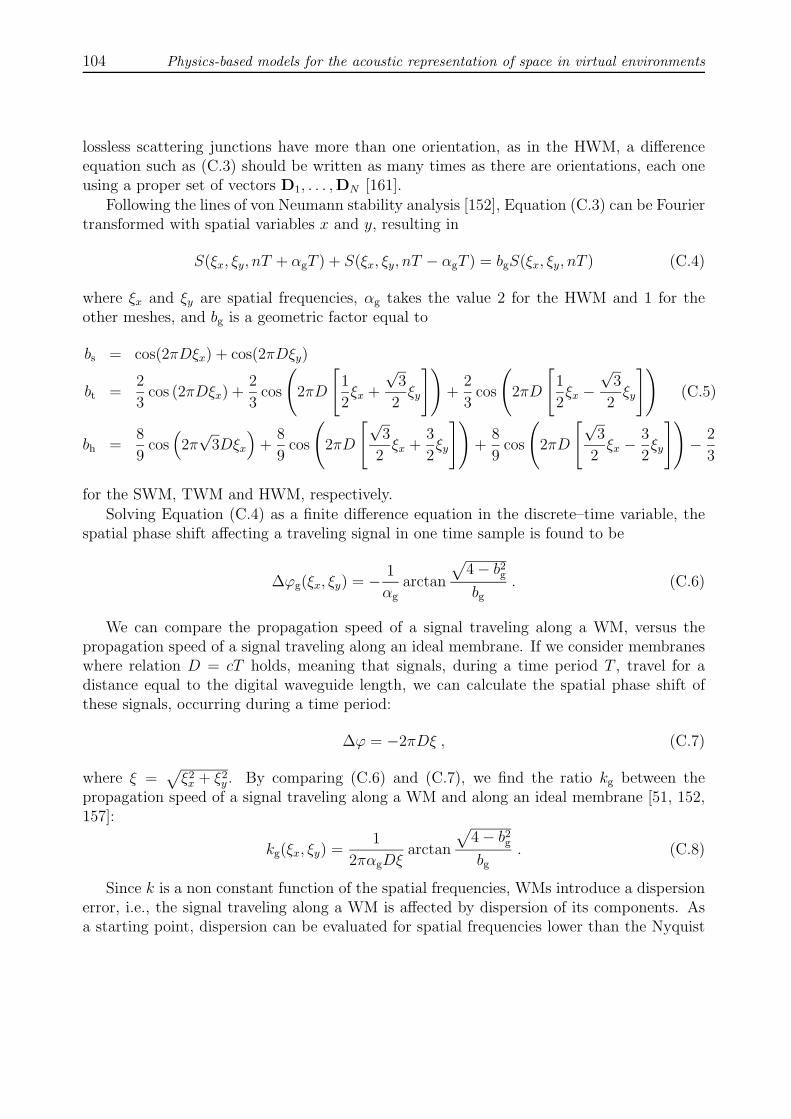
104 Physics-based models for the acoustic representation of space in virtual environments
lossless scattering junctions have more than one orientation, as in the HWM, a differenceequation such as (C.3) should be written as many times as there are orientations, each oneusing a proper set of vectors D1, . . . ,DN [161].
Following the lines of von Neumann stability analysis [152], Equation (C.3) can be Fouriertransformed with spatial variables x and y, resulting in
S(ξx, ξy, nT + αgT ) + S(ξx, ξy, nT − αgT ) = bgS(ξx, ξy, nT ) (C.4)
where ξx and ξy are spatial frequencies, αg takes the value 2 for the HWM and 1 for theother meshes, and bg is a geometric factor equal to
bs = cos(2πDξx) + cos(2πDξy)
bt =2
3cos (2πDξx) +
2
3cos
(2πD
[1
2ξx +
√3
2ξy
])+
2
3cos
(2πD
[1
2ξx −
√3
2ξy
])(C.5)
bh =8
9cos(
2π√
3Dξx
)+
8
9cos
(2πD
[√3
2ξx +
3
2ξy
])+
8
9cos
(2πD
[√3
2ξx −
3
2ξy
])− 2
3
for the SWM, TWM and HWM, respectively.Solving Equation (C.4) as a finite difference equation in the discrete–time variable, the
spatial phase shift affecting a traveling signal in one time sample is found to be
∆ϕg(ξx, ξy) = − 1
αg
arctan
√4− b2
g
bg
. (C.6)
We can compare the propagation speed of a signal traveling along a WM, versus thepropagation speed of a signal traveling along an ideal membrane. If we consider membraneswhere relation D = cT holds, meaning that signals, during a time period T , travel for adistance equal to the digital waveguide length, we can calculate the spatial phase shift ofthese signals, occurring during a time period:
∆ϕ = −2πDξ , (C.7)
where ξ =√ξ2x + ξ2
y . By comparing (C.6) and (C.7), we find the ratio kg between thepropagation speed of a signal traveling along a WM and along an ideal membrane [51, 152,157]:
kg(ξx, ξy) =1
2παgDξarctan
√4− b2
g
bg
. (C.8)
Since k is a non constant function of the spatial frequencies, WMs introduce a dispersionerror, i.e., the signal traveling along a WM is affected by dispersion of its components. Asa starting point, dispersion can be evaluated for spatial frequencies lower than the Nyquist

Chapter C. Signal-Theoretic Characterization of Waveguide Mesh Geometries for Models ofTwo–Dimensional Wave Propagation in Elastic Media 105
(a) (b) (c)
−0.5
0
0.5
−0.5
0
0.50
0.1
0.2
0.3
0.4
0.5
0.6
0.7
0.8
spatial frequency
SWM
spatial frequency
prop
. spe
ed
−0.5
0
0.5
−0.5
0
0.50
0.1
0.2
0.3
0.4
0.5
0.6
0.7
0.8
spatial frequency
TWM
spatial frequencypr
op. s
peed
−0.5
0
0.5
−0.5
0
0.50
0.1
0.2
0.3
0.4
0.5
0.6
0.7
0.8
spatial frequency
HWM
spatial frequency
prop
. spe
ed
Figure C.2: Propagation speed ratios in the SWM (a), TWM (b) and HWM (c), versusdomain given by (C.9).
limit1, that is, in the frequency domain:(ξx, ξy) : |ξx| <
1
2D, |ξy| <
1
2D
. (C.9)
This domain will be refined, according with the considerations to be presented in section C.3.
Figure C.2 shows plots of ks, kt and kh, where D has been set to unity. It can be noticedthat the propagation speed decreases for increasing spatial frequencies. In particular, ks ismaximum when ξx = ξy, and minimum for high values of the spatial frequencies locatedalong the main axes, suggesting that dispersion in the SWM does not affect the diagonalcomponents traveling along it. On the contrary, the HWM exhibits the flattest dispersionerror on the region centered around dc. Finally, the TWM seems to have the most uniformbehavior of the dispersion error.
The propagation speed in all the WMs has a maximum at dc:
kg(0)4= lim
ξ→0kg(ξ) =
1√2
. (C.10)
It is worth noticing that this value corresponds with the nominal propagation speed of asignal traveling along a finite difference scheme [152].
1For the purpose of this paper, the Nyquist limit is defined as half the sample rate, both in time andspace. In some previous works [161, 137] the simulations were considered valid up to a quarter of the samplerate because in the square mesh the frequency response repeats itself after that limit. However, as it waspointed out in [161], this is due to the fact that all transfer functions definable at any one junction arefunctions of z−2. This does not imply that the response to a signal having components up to half the samplerate will be aliased. However, for certain applications such as modal analysis of physical membranes, thefrequency response at quarter of the sample rate is the definitive limit with the square mesh.

106 Physics-based models for the acoustic representation of space in virtual environments
C.2.2 Sampling Lattices
The evaluation of the dispersion error does not give a complete description of the con-straints holding when an ideal membrane is modeled using WMs. In particular, a methodis needed for computing the signal bandwidth a WM is able to process. The theory of sam-pling lattices [42, 156], that we are briefly reviewing in this section, gives the background forcharacterizing WMs from this viewpoint.
Let us sample a 2D continuous signal s over a domain L, subset of R2, so defining adiscrete signal sL(x) , x ∈ L. If L can be described by means of a nonsingular matrixL such that each element of the domain is a linear combination of the columns of L, thecoefficients being signed integers:
x = L
[u1
u2
], u1 ∈ Z , u2 ∈ Z , (C.11)
then L is called a sampling lattice, and L is its basis.
The number of samples per unit area is [42, 156]:
DL =1
det(L), (C.12)
as L contains information about the distance between adjacent samples.
SL, the Fourier transform of sL, is defined over R2 and obtained by periodic imaging ofS, Fourier transform of s. These Fourier images are centered around the elements of thelattice L∗, which is described by the basis L−T , inverse transposed of L. Notice that thedenser the sampling of s is, the sparser the image centers are. In formulas,
DL∗ =1
det(L−T )= det(L) =
1
DL. (C.13)
Let us consider an ideal, unlimited membrane traveled by a spatially band limited signals(x, y, t), and let us do a spatial sampling of the signal, at a given time. Whenever thespatial sampling defines a sampling lattice L, so that sL is defined, we can calculate SL usingthe above results. The multidimensional sampling theorem [42] — which, in brief, tells thatif the Fourier images of s do not intersect one with each other, s can be recovered from sLwith no aliasing error — indicates whether the chosen sampling scheme induces aliasing.
Equation (C.13) tells that for each choice of the sampling lattice geometry, the densityDL can be increased until the images do not intersect. Conversely, given s, there exists asampling lattice capable to capture all the information needed to recover the original signalusing the least density of samples. Clearly, it will exhibit the highest sampling efficiency.

Chapter C. Signal-Theoretic Characterization of Waveguide Mesh Geometries for Models ofTwo–Dimensional Wave Propagation in Elastic Media 107
C.3 Sampling efficiency of the WMs
Sampling efficiency will be calculated for signals having circular spatial band shape cen-tered around the origin of the frequency axes2, with radius equal to B. Even if the analysisprocedure does not depend on the shape of the spatial domain, the circular band seems toinclude all the signals occurring in practical applications. Indeed, the procedure is indepen-dent of the system evolution — which in the WMs is controlled by Equation (C.2) — so thatit applies to any model discretizing distributed systems, and where signal information canbe located over a sampling lattice. This is the case, for example, in finite difference schemes.
C.3.1 WMs and Sampling Lattices
A SWM, having digital waveguides of length Ds, corresponds to a sampling scheme overthe lattice Ls(Ds), described by the basis
Ls(Ds) =
∣∣∣∣ Ds 00 Ds
∣∣∣∣ . (C.14)
A TWM, having digital waveguides of length Dt, corresponds to a sampling scheme over thelattice Lt(Dt), described by the basis
Lt(Dt) =
∣∣∣∣ Dt12Dt
0√
32Dt
∣∣∣∣ . (C.15)
Notice that a triangular scheme is denser than a square scheme made with digital waveg-uides of the same length. This is confirmed by relation
DLt(D)
DLs(D)
=det(Ls(D))
det(Lt(D))=
D2
√3
2D2
=2√3. (C.16)
The description of an HWM having digital waveguides of length Dh, again can be givenin terms of sampling lattices, with some extra care. The HWM is obtained by subtractinga TWM, whose junctions lie on the sampling lattice LT(Dh), from a denser TWM havingjunctions on Lt(Dh). Hence, the junctions of the HWM lie on
Lh(Dh)4= Lt(Dh) \ LT(Dh) . (C.17)
The basis of LT(Dh) is
LT(Dh) =
∣∣∣∣ 32Dh 0√3
2Dh
√3Dh
∣∣∣∣ . (C.18)
Figure C.3 shows the HWM over Lh(Dh), obtained by subtracting the sampling latticeLT(Dh) (whose elements are depicted with ×) from Lt(Dh) (elements depicted with •).
2This class of signals encompasses the signals obtained when a membrane is excited, in one or severalpoints, by a single shot or by a sequence of shots, using a stick with an approximately round tip.

108 Physics-based models for the acoustic representation of space in virtual environments
Dh Dh21
Dh32
x
y
Figure C.3: The HWM, obtained by subtraction of TWMs. × are elements belonging toLT(Dh), • are elements belonging to Lt(Dh).
C.3.2 TWM vs SWM
The image centers of the spectra belonging to signals traveling along a SWM and a TWMare respectively described by the basis matrices of L∗s and L∗t :
Ls(Ds)−T =
∣∣∣∣ 1/Ds 00 1/Ds
∣∣∣∣ , (C.19)
and
Lt(Dt)−T =
∣∣∣∣ 1Dt
0
− 1√3
1Dt
2√3
1Dt
∣∣∣∣ . (C.20)
Figure C.4 shows Fourier images for the SWM (empty circles in dashed line) and theTWM (filled circles), located around the origin of the frequency plane. It can be noticed thatthe square sampling scheme induces a square positioning of the images and, consequently, asquare tiling of the frequency plane, as emphasized by the square in dashed line. Similarly,sampling over a TWM results in a triangular positioning of the images, thus producing anhexagonal tiling of the frequency plane, as shown by the hexagon located over the center.Such hexagonal tiling allows, as it appears quite evidently in the figure, to “pack” the imagesbetter than those coming from a square sampling.
When both a SWM and a TWM critically sample the same signal (i.e. the filled circlestouch each other without intersecting, and the same thing happens for the empty circles), itis easy to derive the following relation between the digital waveguide lengths:
Dt
Ds
=2√3≈ 1.134 . (C.21)

Chapter C. Signal-Theoretic Characterization of Waveguide Mesh Geometries for Models ofTwo–Dimensional Wave Propagation in Elastic Media 109
12
31 1
Dt
ξx
yξ
1Ds
Figure C.4: Domains of Fourier images in a SWM (empty circles in dashed line) and ina TWM (filled circles), and the correspondent tiling induced by the respective geometries(square in dashed line and hexagon in solid line). The empty and the filled circles have thesame radius and touch each other without intersecting, meaning that both the SWM andthe TWM critically sample the same signal.
Under this condition we can relate the sample densities in the two geometries:
DLt(Dt)
DLs(Ds)
=DLt(
2√3Ds)
DLs(Ds)
=det(Ls(Ds))
det(Lt(2√3Ds))
=
√3
2, (C.22)
concluding that the TWM exhibits a better sampling efficiency relative to the SWM. In otherwords, a signal can be spatially sampled with a triangular geometry using 13.4% less samplesper unit area.
C.3.3 TWM vs HWM
Said sh and st the signals sampled over the junctions of the HWM and the TWM,respectively, and said sT the signal sampled over the lattice LT(Dh), we can define thezero-padded signals
sT(x) =
0 , x ∈ Lh(Dh)sT(x) , x ∈ LT(Dh)
(C.23)
and
sh(x) = st(x)− sT(x) =
sh(x) , x ∈ Lh(Dh)0 , x ∈ LT(Dh)
(C.24)

110 Physics-based models for the acoustic representation of space in virtual environments
ξx
yξ
31 1
Dh
D12
3 h
Figure C.5: Centers (×) of the Fourier images coming from a TWM defined by Lt(Dh),and centers (•) of the Fourier images coming from a sparser TWM defined by LT(Dh).Subtraction of × from • gives the centers of the Fourier images (located on the filled circles)coming from an HWM defined by Lh(Dh). The respective tiling is given by the triangles.Both the HWM and the sparser TWM critically sample the same signal.
Since we cannot define a Fourier transform over Lh(Dh), we consider Sh, Fourier transformof sh (which is defined over Lt(Dh)), as a description of sh in the frequency domain. Sh,according to its definition, can be obtained by subtracting ST from St:
Sh(ξx, ξy) = St(ξx, ξy)− ST(ξx, ξy) . (C.25)
The result is shown in Figure C.5, where some images of ST are depicted (filled circles pluscircle in dashed line). The elements of LT
∗(Dh) are marked with •, while the elements ofLt∗(Dh) are marked with ×.The HWM induces an hexagonal positioning of the Fourier images (corresponding to
the filled circles). In fact, their centers are elements of a set which, again, can be definedby a subtraction between two sampling lattices, Lt
∗(Dh) and LT∗(Dh), which are recipro-
cal of Lt(Dh) and LT(Dh), respectively. The consequent tiling geometry is triangular, asemphasized by the triangles depicted in Figure C.5.
It can be observed that image intersection does not occur in Lh(Dh) if and only if s issampled without aliasing over LT(Dh). In other words, when ST exhibits superposition ofits images, the same thing happens for the images of Sh, and vice versa.
Moreover, it must be noticed that equation
LT(Dh) = Lt(√
3Dh) (C.26)

Chapter C. Signal-Theoretic Characterization of Waveguide Mesh Geometries for Models ofTwo–Dimensional Wave Propagation in Elastic Media 111
holds between LT and Lt, if a rotation is neglected. This relation, together with the consid-erations about image superposition made just above, allows us to say that an HWM doesnot perform better than a TWM, whose digital waveguides are
√3 times longer.
Another interesting consideration comes out by noticing that, since
DLt(Dh)
DLT(Dh)
=det(LT(Dh))
det(Lt(Dh))= 3 , (C.27)
then the TWM defined over the lattice LT(Dh) is 3 times as sparse as the TWM defined overLt(Dh), thus (directly from the definition of Lh) 2 times as sparse as the HWM. Hence, thenumber of lossless scattering junctions per unit area of the HWM is twice as high as that ofthe TWM defined over LT(Dh), with no benefits on the accuracy of sampling. This relateswith the fact that the hexagons tiling the frequency plane (as the inner hexagon depicted inFigure C.5) contain twice the information needed to recover s correctly: the 6 partial imagesincluded in the slices inside the central hexagon can be composed into 2 Fourier images.
C.4 Signal time evolution
In this section, we discuss the consequences of critical spatial sampling on the temporalsampling frequency.
First, let us consider the sampled version of a signal traveling at speed c along an idealmembrane that has been excited by a bandlimited signal f(x, y) having Fourier transformequal to F (ξx, ξy). It can be shown (see Appendix A) that a time sampling frequency
Fs = 2c maxξ:|F (ξ)|6=0
ξ (C.28)
is required to recover the original signal correctly.When such a signal has a spatial circular band shape, thus belonging to the class seen in
section C.3, the relationmax
ξ:|F (ξ)|6=0ξ = B (C.29)
holds, so that Equation (C.28) simplifies into
Fs = 2cB . (C.30)
Relation (C.30) has an immediate physical interpretation: waves having wavelength equal to1/B, propagating at speed c along a medium, exhibit a temporal frequency equal to cB. Inorder to preserve information in their sampled versions, they must be sampled above twicetheir frequency.
The value given by Equation (C.30), if used as the sampling frequency of a 2D-resonatormodel (realized by means of WMs having critical waveguide lengths), causes inaccuratepositioning of the modal frequencies. Assumed that dispersion (see section C.2.1) cannot in

112 Physics-based models for the acoustic representation of space in virtual environments
general be eliminated, as it is a consequence of the finite number of directions a 2D signalcan propagate along a WM3, the propagation speed can at least be set to its physical valuein low frequency. This can be done by simply rescaling Fs according to the geometry.
Recalling the procedure leading to Equation (C.7), we can reformulate the spatial phaseshift of a signal traveling along the ideal membrane, during a time period T = 1/Fs. Hence,we find the following expression for the ratio (C.8), reformulated using for each geometry itsrespective critical waveguide length:
kg(ξx, ξy) =1
2παgDξarctan
√4− b2
g
bg
, (C.31)
where bg has the structure of bg (see Equation (C.5)), but the waveguide length D has beenreplaced by its critical counterpart Dg.
Recalculation of the limit (C.10) gives:
kg(0) =Dg
Dkg(0) =
1√2
Dg
D, (C.32)
that is, considering Ds as the reference waveguide length,
ks(0) =1√2, kt(0) =
√2√3, kh(0) =
√2
3. (C.33)
This result shows that signals, under conditions of critical sampling, propagate in theWMs at different speeds, according to the geometry. The dispersion ratios can be set tounity at dc by using the temporal sampling frequencies
F s,g =1
kg(0)Fs . (C.34)
For the purpose of Section C.5, the dispersion ratio of a critically sampled 2D medium,adjusted to be one at dc, is called kg(ξx, ξy).
C.5 Performance
In order to compare the three geometries under critical sampling conditions, we show inFigure C.6 the contour plots of kg, for a nominal spatial bandwidth B = 1/2 (correspondingto the circle in the figure).
3Savioja and Valimaki [137] have pointed out that a signal, coming out from a TWM, can be frequencywarped to reduce the dispersion error. This is made possible by the fact that kt(ξx, ξy) can be approximatedwith a single–variable function kt(ξ).

Chapter C. Signal-Theoretic Characterization of Waveguide Mesh Geometries for Models ofTwo–Dimensional Wave Propagation in Elastic Media 113
(a) (b) (c)
−0.5 −0.4 −0.3 −0.2 −0.1 0 0.1 0.2 0.3 0.4 0.5−0.5
−0.4
−0.3
−0.2
−0.1
0
0.1
0.2
0.3
0.4
0.5
0.8
0.9
0.95
Normalized spatial frequency
Norm
aliz
ed s
patial fr
equency
SWM
−0.5 −0.4 −0.3 −0.2 −0.1 0 0.1 0.2 0.3 0.4 0.5−0.5
−0.4
−0.3
−0.2
−0.1
0
0.1
0.2
0.3
0.4
0.5
0.8
0.9
0.95
Normalized spatial frequency
Norm
aliz
ed s
patial fr
equency
TWM
−0.5 −0.4 −0.3 −0.2 −0.1 0 0.1 0.2 0.3 0.4 0.5−0.5
−0.4
−0.3
−0.2
−0.1
0
0.1
0.2
0.3
0.4
0.5
0.9
0.95
Normalized spatial frequency
Norm
aliz
ed s
patial fr
equency
HWM
Figure C.6: Contour plots of propagation speed ratios in the SWM (a), TWM (b) and HWM(c), when temporal sampling frequency has been set to F s,g. All the WMs process a signalhaving bandwidth (depicted with the circle) equal to 1/2.
It can be noted that the behaviors of the SWM and the TWM are not dramatically differ-ent in terms of average dispersion error: dispersion stands quite below 20% for most spatialfrequencies in both the geometries. However, the TWM exhibits a more uniform behavior,and this uniformity can be exploited using frequency warping [137]. Conversely, dispersionin the HWM stays below 10% almost everywhere, thus indicating that this geometry has themost uniform propagation speed under these test conditions.
The computational cost and the memory requirement in the different geometries can becalculated under the same conditions. They are based on Equation (C.2) which shows thateach N–port lossless scattering junction requires 2N operations to compute the wave signalscoming out from the junctions, to be stored into N locations belonging to the adjacent digitalwaveguides. These operations amount to 2N−1 additions, and 1 multiplication (which canbe replaced by a bit shift in fixed–point implementations of the SWM).
Table C.1 summarizes the performance, when the reference sampling rate of the squaremesh F s,s has been set to a nominal value equal to unity. Numbers are given for twoimplementations: as a waveguide mesh (with memory in the waveguide branches), and as afinite difference scheme (with memory in the junctions).
The numbers of operations and memory locations per junction for the WM follow directlyfrom Equation (C.2). The numbers of operations and memory locations per junction for thefinite difference scheme follow directly from Equation (C.3). The densities of junctions resultfrom Equations (C.21) and (C.26). The densities of locations are obtained by multiplyingthe third row times the fourth row. The sample rates are a consequence of Equation (C.34).
The results of table C.1 show that the triangular finite difference scheme uses the leastquantity of memory. Among WM implementations, the SWM is the most efficient in termsof memory occupation.

114 Physics-based models for the acoustic representation of space in virtual environments
Waveguide Finite DifferenceMesh Scheme
Sq. Tr. Hex. Sq. Tr. Hex.
additions per junction 7 11 5 4 6 3multiplications per junction 1 1 1 1 1 1
memory locations per junction 4 6 3 2 2 2density of junctions 1 0.866 1.732 1 0.866 1.732
density of memory locations 4 5.2 5.2 2 1.732 3.464sample rate 1 0.866 1.5 1 0.866 1.5
additions per unit time and space 7 8.25 12.990 4 4.5 7.794multiplications per unit time and space 1 0.75 2.598 1 0.75 2.598
Table C.1: Performance of the geometries in terms of memory requirement and compu-tational cost (multiplications are pure bit–shifts in the SWM). Two implementations areconsidered: as a waveguide mesh and as a finite difference scheme.
Finally, the number of additions (multiplications) per unit time and space results bymultiplication of the number of additions (multiplications) per junction, density of junctions,and sample rate. Once again, the SWM has the least density of operations when a WMmodel is required. Conversely, the square and the triangular geometries have about thesame computational requirements in a finite difference implementation.
C.5.1 Numerical example
Let us design a WM, capable of modeling in real–time an ideal 2D round resonator, ofradius r = 0.1 m, where waves propagate at a speed c equal to 130 m/s. Let the signalcontain information up to a frequency f = 10 kHz.
The spatial bandwidth B of the signal traveling along the resonator is:
B =f
c=
10000 Hz
130 m/s= 76.923 m−1 , (C.35)
and consequently the critical waveguide lengths required to model the signal, in the respectivegeometries, are:
Ds =1
2B= 6.5 mm ;
Dt =1√3B
= 7.5 mm ; (C.36)
Dh =1
3B= 4.3 mm .

Chapter C. Signal-Theoretic Characterization of Waveguide Mesh Geometries for Models ofTwo–Dimensional Wave Propagation in Elastic Media 115
This means that the numbers of junctions — Ns, Nt and Nh, respectively — needed in thethree models are4
Ns ≈πr2
D2s
= 744 ;
Nt ≈πr2
√3
2D2
t
= 645 ; (C.37)
Nh ≈2
3
πr2
√3
2D2
h
= 1308 .
The time sampling frequencies needed to have kg(0) = 1 are, from Equation (C.34):
F s,s = 2√
2f = 28.285 kHz ;
F s,t = 2
√3
2f = 24.495 kHz ; (C.38)
F s,h = 23√2f = 42.427 kHz .
C.6 Conclusion
A novel wave propagation model has recently been introduced for the simulation ofisotropic multidimensional media. It makes use of structures called waveguide meshes. Evenif most of the waveguide mesh properties have already been understood, there was lack ofliterature about their performance from a signal–sampling viewpoint.
In this paper, some properties of the most common 2D waveguide meshes — square,triangular and hexagonal — related with the bandwidth of the signal traveling on them,have been inspected. In particular, it has been shown that the triangular waveguide meshis capable of processing a larger bandwidth than the square or hexagonal waveguide mesheshaving the same digital waveguide lengths.
Furthermore, when processing signals of the same bandwidth, the triangular waveg-uide mesh does not exhibit a computational and memory load much larger than the mostcomputationally–efficient waveguide mesh — the square mesh — such that it can be con-sidered, for the uniformity of its dispersion error, a good choice both in terms of simulationerrors and computational cost.
The analysis presented in this article may be extended to 3D media, comparing thethree geometries which most directly correspond to the waveguide meshes here reviewed: 3Drectilinear, dodecahedral, and tethraedral.
4The values result by calculating the number of small areas, each one being associated with its ownlossless scattering junction, which tessellate the resonator.

116 Physics-based models for the acoustic representation of space in virtual environments
C.7 Acknowledgment
We would like to thank Lauri Savioja and Vesa Valimaki for many insightful discussions.We are also grateful to the anonymous reviewers for their constructive criticism.
C.8 Appendix - Sampling of a signal traveling along
an ideal membrane
An ideal membrane establishes a relation between the spatial Fourier transforms of thesignal s traveling on it, taken in correspondence of two times, t and t:
S(ξx, ξy, t) = ej2πc(t−t)ξ S(ξx, ξy, t) . (C.39)
This relation has the following interpretation: each spatial component of the signal, travelingalong a distance equal to c(t − t) during time (t, t), has no magnitude variation, and hasphase variation equal to −c(t− t)ξ [157].
Let us excite, at time t, the ideal membrane with a spatially band limited signal f(x, y)having Fourier transform F (ξx, ξy). The application of (C.39) gives the spatial Fourier trans-form of the signal on the membrane:
S(ξx, ξy, t) =
0 , t < t
ej2πc(t−t)ξ F (ξx, ξy) , t ≥ t(C.40)
From this relation, we can calculate the critical temporal sampling frequency required tosample, without loss of information, a signal traveling on an ideal membrane. In fact, theFourier transform of the signal calculated by its spatial Fourier transform,
S(ξx, ξy, f) =
∫ +∞
−∞S(ξx, ξy, t)e
−j2πft dt , (C.41)
has a magnitude equal to
|S(ξx, ξy, f)|
=
∣∣∣∣∫ +∞
−∞S(ξx, ξy, t)e
−j2πft dt
∣∣∣∣=
∣∣∣∣∫ +∞
t
ej2πc(t−t)ξ F (ξx, ξy)e−j2πft dt
∣∣∣∣ (C.42)
=
∣∣∣∣∫ +∞
t
e−j2πctξ F (ξx, ξy)e−j2πtf−cξ dt
∣∣∣∣= |F (ξx, ξy)|
∣∣∣∣∫ +∞
t
e−j2πtf−cξ dt
∣∣∣∣ .

Chapter C. Signal-Theoretic Characterization of Waveguide Mesh Geometries for Models ofTwo–Dimensional Wave Propagation in Elastic Media 117
In particular, when t→ −∞ :
|S(ξx, ξy, f)|
= |F (ξx, ξy)| limt→−∞
∣∣∣∣∫ +∞
t
e−j2πtf−cξ dt
∣∣∣∣ (C.43)
= |F (ξx, ξy)|∣∣∣∣∫ +∞
−∞e−j2πtf−cξ dt
∣∣∣∣= |F (ξx, ξy)| δ(f − cξ) .
This means that some spectral power exists for any temporal frequency (equal to cξ) asso-ciated to a spatial component of frequencies (ξx, ξy) excited in the membrane. Invoking thesampling theorem [110], the critical time sampling frequency Fs results to be equal to (C.28).

118 Physics-based models for the acoustic representation of space in virtual environments

Appendix D
A Modified Rectangular WaveguideMesh Structure with InterpolatedInput and Output Points
Federico Fontana, Lauri Savioja and Vesa ValimakiProc. International Computer Music Conference, pages 87–90, La Habana, Cuba, September 2001.
The rectangular waveguide mesh presents aspects of redundancy when computing the impulseresponse of an ideal resonator. Its structure is thus modified, to define a new structure whereredundant computations and unnecessary memory consumption are removed. The modifiedmesh saves half of the memory and computations, meanwhile it preserves all the numericalproperties of the rectangular waveguide mesh accounting for stability, direction-dependentpropagation speed of the wavefronts and so on. A general method, which is derived bybilinear interpolation and deinterpolation, is adapted for generalizing the input/output pointpositions in the modified structure. Simulations confirm the conjectures advanced herein.
D.1 Introduction
Waveguide meshes [158], in their several formulations, are deserving a certain attentionby researchers concerned with the design of resonators for musical, audio and multimediaapplications. Previous studies [50, 138], for instance, have inspired some interesting applica-tions of the waveguide mesh (from now denoted as WM) for modeling percussion instruments[51, 2], string instrument bodies [74], and in the analysis of reverberant enclosures [134, 106].
Although some formulations of the WM allow to realize models that closely approachthe behavior of an ideal resonator, the original structure [158] remains a valuable trade-off between computational efficiency and versatility. Moreover, it allows a straightforwardimplementation, and this is very useful at least when one conducts preliminary tests ofreliability of a WM model with respect to a given modeling problem.
119

120 Physics-based models for the acoustic representation of space in virtual environments
In that case, minimizing the computational cost of the procedure is often an importantissue. Any redundancy introduced in the computations by a heavier implementation of themodel translates into unnecessary hardware usage, and longer wait for the output. Thisis true especially when the WM is used in problems involving accurate modeling of hugeresonators: in this case, processing time and memory consumption often become a criticalfactor.
The rectangular (square) WM (SWM from now) exhibits this redundancy. This can benoted, for example, by analyzing the spectrum of its magnitude response: such a responsein fact mirrors at half of the Nyquist frequency, independently from where the impulse isinjected and the response is taken, suggesting that half of the computations performed duringthe calculation of this response are unnecessary. We show that, in these cases, an SWM canbe turned into a similar, lighter structure saving half of the memory and computations. Inspite of this, the performance of the SWM is preserved, since only redundant information isremoved by the modified structure.
Moreover, a method to calculate the output in correspondence of a point that is mis-aligned from the junction positions is proposed, together with a strategy for injecting asignal when the input position differs from any scattering point position. Such a gener-alized excitation and acquisition points can be obtained by applying bilinear interpolationto the existing scattering points in the modified SWM [136]. Though, the interpolationand deinterpolation formulas must be rewritten for accommodating them to the modifiedstructure.
An alternative treatment of these arguments, based on the theory of Digital WaveguideNetworks, will be cited whenever it has contributed to inspire this research, and when theconclusions are similar [13]. Rather, the background of the present work is more focused onthe theory of audio signals.
D.2 A Modified SWM
The impulse response of an SWM is known to present redundant information, in a waythat its spectrum mirrors at half of the Nyquist frequency. This characteristic does notdepend on the position of the junction where the impulse is fed, and the position from wherethe response is taken. From a signal-theoretic viewpoint, this descends from the fact thatthe discrete-time transfer function which describes the response of the SWM with respectto the input and output positions is always a function of the variable z−2 [158]. Since thisproperty comes from the numerical scheme which is computed by the mesh, it appears alsoin a realization made adopting a Finite Difference Scheme.
This issue has been outlined also by Bilbao [13], who shows that the SWM can besubdivided in two mutually exclusive schemes. Their independence comes from the fact thatthe SWM processes two subsets of data at each time sample, and never performs any kindof merging between them. As a result, a sample which is taken from one scattering point ata given time step does not have structural relations with the sample which is taken at the

Chapter D. A Modified Rectangular Waveguide Mesh Structure with Interpolated Input andOutput Points 121
z−1
z−1
z−1
z−1z−1
z−1
z−1
z−1
z−1
z−1
z−1 z−1
z−1z−1 z−1
z−1 z−1
z−1
z−1
z−1
z−1
z−1
z−1
z−1
Figure D.1: Modified SWM (size 5×5) having reflecting edges. • are scattering junctionsbelonging to S2n. are scattering junctions belonging to S2n+1. Junctions at the boundaryreverse the sign of the incoming waves.
previous (or following) time step from the same point.
The excitation in general establishes a mutual dependence between adjacent samples, sothat the output from the SWM is in most cases informative over the whole spectrum. Inspite of this, there are situations where one of the two subsets becomes unnecessary. Inparticular, the impulse response comes from the excitation of only one of them, hence thespectral content coming from the samples belonging to the latter subset, which are alwaysequal to zero, is redundant.
Consider an SWM as a connection of objects, each one made of one N -port scatteringjunction and N outgoing branches containing one unit delay1. Now, modify the mesh struc-ture by interleaving these objects with new ones, where the unit delays have been substitutedby delay-free connections. Denote the set containing the former objects with S2n+1, and letS2n be the set containing the new ones. Figure D.1 depicts the structure resulting from anSWM of size 5×5 having perfect reflection at the boundaries.
At each time step, junctions belonging to S2n compute the signal in the same way as ithappens in the normal SWM. Yet, wave signals are sent without delay back to the junctionsbelonging to S2n+1. Hence, samples which do not keep information are overwritten with
1Clearly, it will be N = 4 for the SWM, and N = 6 for the 3-D rectangular WM [134].

122 Physics-based models for the acoustic representation of space in virtual environments
t/T
2n+1
2n
Figure D.2: Interpretation of the signal generated by the modified SWM. Samples producedby the junctions in S2n+1 follow the samples produced by the junctions in S2n.
values that, in the normal SWM, are computed during the following time step (see FigureD.2).
The stability and propagation properties of the modified structure are the same as inthe SWM, since the numerical scheme realized by the modified mesh includes the schemecomputed by the SWM. From a signal-theoretic viewpoint, the information which is presentin the modified structure equals the information conveyed by the SWM.
The modified SWM is convenient whenever the excitation signal mirrors at half of theNyquist frequency. Under this assumption, the global amount of memory in the new struc-ture is halved, while the number of operations needed to calculate the output is in principlethe same. Though, considering that two time samples of the output are calculated duringeach computation cycle, the number of operations that are needed to compute the outputsignal is reduced by a factor of two as well. Such a convenience appears in an FDS realizationof the modified scheme as well. In this case, the reduction in memory consumption appearsin the form of just one unit delay associated with each scattering point, instead of two.
Simulations conducted over the two models confirm that the spectral redundancy presentin the magnitude response of the SMW (Figure D.3) is removed by the modified structure(Figure D.4).

Chapter D. A Modified Rectangular Waveguide Mesh Structure with Interpolated Input andOutput Points 123
0 0.1 0.2 0.3 0.4 0.5−50
−40
−30
−20
−10
0
10
20
Normalized frequency
dB
Figure D.3: Frequency response of a SWM (size 25×25). Excitation at the center.
D.3 Interpolated Input and Output Points
The modified structure can be excited in correspondence of the junctions belonging toS2n+1. Likewise, each one of these junctions presents the impulse response calculated incorrespondence of its own position. In spite of this, there are cases where the excitation oracquisition points cannot correspond with the positions of the scattering points.
In these cases, first-order Lagrange interpolation can be used to interpolate betweenjunctions. This method can be extended to the two-dimensional case in the form of bilinearinterpolation, whose versatility and ease of use together with the SWM have been previouslyshown [136].
In that treatment, the formulas accounting for coefficients wij that weight the samplessij of the (four) nearest scattering points, namely 11, 12, 21, and 22, are the following ones:
w11 = (1− x)(1− y) , w12 = x(1− y)
w21 = (1− x)y , w22 = xy
where (x, y) are the coordinates of the interpolated output v relative to position 11:
v(x, y) =2∑i=1
2∑j=1
wijsij
The same weighting parameters are used to deinterpolate the input u(x, y) over the nearestscattering points:
sij = wij u(x, y)

124 Physics-based models for the acoustic representation of space in virtual environments
0 0.1 0.2 0.3 0.4 0.5−50
−40
−30
−20
−10
0
10
20
Normalized frequency
dB
Figure D.4: Frequency response of a modified SWM (size 25×25). Excitation at the center.
All these formulas hold when the digital waveguide lengths have been normalized to unity.
Such relations apply also to the junctions belonging to S2n+1 in the modified structure,once they are reformulated (see Figure D.5) in new coordinates (x∗, y∗). This transformation
xEW
N
S
y
*
*
x
y
22
(a) (b)
21
11 12
Figure D.5: Reformulation of bilinear interpolation from original (a) to new (b) coordinatesobtained by translating, rotating and stretching the old set.
consists of a translation by (−1/2,−1/2) followed by a rotation by π/4. The new coordinatesare finally stretched by a factor equal to
√2. New weighting parameters are thus found out,

Chapter D. A Modified Rectangular Waveguide Mesh Structure with Interpolated Input andOutput Points 125
0 0.1 0.2 0.3 0.4 0.5−50
−40
−30
−20
−10
0
10
20
Normalized frequency
dB
Figure D.6: Spectrum from deinterpolated excitation around the center of a modified SWMsized 25×25 (solid line) compared with spectrum depicted in Figure D.4 (dashed line).
with the notations depicted in Figure D.5(b):
wN = (1− x∗ + y∗)(1 + x∗ + y∗)/4
wW = (1− x∗ + y∗)(1− x∗ − y∗)/4wE = (1 + x∗ − y∗)(1 + x∗ + y∗)/4
wS = (1 + x∗ − y∗)(1− x∗ − y∗)/4
Suppose, for example, to swap S2n+1 and S2n in the square structure that produces thespectrum depicted in Figure D.4; we obtain a new, square mesh that is centered arounda junction belonging to S2n, like the one depicted in Figure D.1. Clearly, in this case anexcitation at the center can no longer be applied. If we excite the center of the mesh usingdeinterpolation over the four neighbors, a response is obtained like the one (in solid line)in Figure D.6, where the non-deinterpolated excitation (refer to Figure D.4) is repeated(in dashed line) for ease of comparison. Note that some amplitude distortion appears,coming from Lagrange interpolation. In this case, distortion is at its maximum since weare interpolating on a point which is farthest from any neighbor scattering junction. Ingeneral cases amplitude distortion is less severe.
Finally, note that (de/)interpolation can be applied, more in general, to any differencescheme whose scattering nodes do not match with the excitation/acquisition point positions.

126 Physics-based models for the acoustic representation of space in virtual environments
D.4 Conclusion
A modified rectangular waveguide mesh has been presented. It processes a numericalscheme which is included by the square waveguide mesh. It saves half of the computationsand memory without loosing any information during the calculation of the impulse response.In the case that the input and output points differ from the junction positions, bilineardeinterpolation and interpolation can be respectively applied to feed the mesh and acquireits response.
The analysis presented in this paper can be easily extended to 3-D rectangular waveguidemeshes and to finite difference schemes.

Appendix E
Acoustic Cues from Shapes betweenSpheres and Cubes
Federico Fontana, Davide Rocchesso and Enzo ApollonioProc. International Computer Music Conference, pages 278–281, La Habana, Cuba, September 2001.
Solids of different shapes resonate according to their peculiar geometry. Although physics,for some fundamental shapes such as the cube and the sphere, provides explicit formulasfor determining the modal frequencies, a general resonance analysis of 3-D shapes must beconducted using numerical methods. In this paper, Waveguide Meshes are used to modelintermediate geometries between the cube and the sphere. This example is paradigmatic ofthe general problem of morphing 3-D shapes.
We are interested in understanding how smooth shape transitions from sphere to cubetranslate into a migration of the resonating modes. This work is aimed at assessing thesuitability of the waveguide mesh as a tool for such a research, and it is preliminary tofurther investigations involving human subjects.
E.1 Introduction
Acoustic rendering is an emerging research field, whose growth is stimulated by two,somehow opposite factors: an increasing interest for applications of multi-modal virtualreality on one side, and inevitable constraints in cost and technology of the equipment on theother side. These factors, together, lead to looking for rendering methods which are realisticand computationally efficient at the same time. Under this assumptions, a method whichis capable to acoustically render objects, or enclosures, will move the listener to virtuallyexperience a scenario without reproducing all its characteristics.
Important studies have already been conducted in the visual field, and remarkable resultshave been achieved in rendering shadows, textures, lightings, and object movement. Thisencourages to looking for audio counterparts of those methods.
127

128 Physics-based models for the acoustic representation of space in virtual environments
Perception of shapes from acoustic cues is a matter of investigation for researchers inpsychophysics [92] and object modeling [127]. A listener could experience, by hearing, tostay for example in the middle of a semi-spherical enclosure, or in front of a large cube,without seeing any of them [96]. Tests have been conducted to investigate whether or notlisteners discriminate simple shapes such as cubes and spheres [127]. Such experiments showthat shape labels can be reliably attached to sounds, regardless of their pitch, and that thedistribution of low-frequency resonances play the prominent role in this task. As a sideresult [128], it was shown that non musicians tend to equalize pitches of resonators as ifthey resulted from equal-volume shapes. This gives us a simple criterion that can be usedto minimize the influence of pitch when experimenting with 3-D objects of varying shapes.
In this work we investigate on the “spectral continuum” holding when a cube morphsinto a sphere, through specific geometries called superquadrics [88]. We look for specificcues to check out if there are “footprints” which acoustically label each intermediate shape,and, hence, the whole morphing process. We will show that these cues exist, although onlylistening tests could demonstrate a real sensitivity of human beings to shape variations.
A numerical method is needed for studying the ellipsoidal shapes. In our work, allresonators are modeled using waveguide meshes [158]. In particular, the 3-D triangularwaveguide mesh (3DTWM) has been adopted, for its low dispersion characteristics andgood approximation in modeling boundaries [54].
All the simulations have been conducted working with an application written in C++,whose user interface can be seen from the screenshot in Figure E.1. This application simplifiesthe construction and initialization of the mesh, and performs all needed processing. A pre-release of the executable program is available from the Web site of the SOb European Project(http://www.soundobject.org) for public experimentation.
E.2 From Spheres to Cubes
One possible morphing from spheres to cubes can be easily realized if we restrict anypossible geometry to be an ellipsoid. Superquadrics are, in this sense, a versatile familywhich is defined by the following equation [88]:∣∣∣x
a
∣∣∣γx +∣∣∣yb
∣∣∣γy +∣∣∣zc
∣∣∣γz = 1 (E.1)
Changes in shape are then performed by varying only the three parameters γ = γx = γy = γztogether, and constraining a, b, c to condition a = b = c :
• sphere: γ = 2
• ellipsoid between sphere and cube: 2 < γ <∞
• cube: γ →∞.

Chapter E. Acoustic Cues from Shapes between Spheres and Cubes 129
Figure E.1: User interface of the application running the mesh models.
We consider six shapes, including the sphere and the cube, which are built according to(E.1). Their positive section (i.e., their volume limited to (x, y, z) : x > 0 , y > 0 , z > 0)is depicted in Figure E.2, where, starting from left above, parameter γ has been set to
γ1 = 2 γ2 = 2.2 γ3 = 2.5
γ4 = 3 γ5 = 4 γ6 = 10
respectively. Note that γ6 is large enough to represent the cube. This is true because thediscrete boundary, which will be modeled by the 3DTWM, does not change for γ ≥ 10.
Accordingly, waveguide mesh models are built. Taking advantage from the applicationpresented above, 3DTWM’s are constructed so that they match, as close as possible, thegeometries coming from the selected ellipsoids. Perfect reflection of the signal holds at theboundary.
Figure E.3 depicts orthogonal projections to the z-plane of the mesh models, in the sameorder given in Figure E.2, for intermediate shapes.
Inevitable mismatching between ideal geometries and 3DTWM models can be noted,even if the scattering junction density was guaranteed to provide a minimum distance equalto 20 junctions between surfaces located on opposite sides.

130 Physics-based models for the acoustic representation of space in virtual environments
0
0.2
0.4
0.6
0.8
1
00.2
0.40.6
0.81
0
0.2
0.4
0.6
0.8
1
0
0.2
0.4
0.6
0.8
1
00.2
0.40.6
0.81
0
0.2
0.4
0.6
0.8
1
0
0.2
0.4
0.6
0.8
1
00.2
0.40.6
0.81
0
0.2
0.4
0.6
0.8
1
0
0.2
0.4
0.6
0.8
1
00.2
0.40.6
0.81
0
0.2
0.4
0.6
0.8
1
0
0.2
0.4
0.6
0.8
1
00.2
0.40.6
0.81
0
0.2
0.4
0.6
0.8
1
0
0.2
0.4
0.6
0.8
1
00.2
0.40.6
0.81
0
0.2
0.4
0.6
0.8
1
Figure E.2: Positive sections of superquadrics obtained using (E.1). γ has been set to2 , 2.2 , 2.5 , 3 , 4 , 10 starting from left above, respectively.
Moreover, the 3DTWM models flat surfaces with lower accuracy due to its own topology.This causes some blur in the definition of the resonance peaks, especially in the case of thecube. This will be evident in the spectral analysis.
E.3 Spectral Analysis
For each geometry, one spectrum was calculated from a signal obtained by exciting (usingan ideal impulse) the resonator on three points, i.e., the center plus two points close tothe boundary. The output signal was picked up on a position which was located near theboundary, for capturing most of the resonances. For non-spherical shapes, the excitation andoutput junctions were located near one corner. Since the corner geometry varies togetherwith shape, inevitable variations in the excitation and acquisition positions occur during theexperiment. For this reason, the dynamics of the output signals varies with shape.
Signals have been damped offline. Offline damping ensures that the resonances do notmove due to imperfect internal modeling of attenuation mechanisms.
Each spectrum should be rescaled in the frequency axis, holding the condition of volumeconstancy. Table E.1 (second column) shows, according to the chosen geometries, volumeratios for resonators having the same size1 in the sense of Figure E.2. In the third column,size ratios for resonators having the same volume are shown. Clearly, frequency rescalings
1say, diameter of the sphere, and side length of the cube

Chapter E. Acoustic Cues from Shapes between Spheres and Cubes 131
Figure E.3: Projections, orthogonal to the z-plane, of 3DTWM models closely matching theintermediate shapes given in Figure E.2. γ has been set to 2.2 , 2.5 , 3 , 4 starting fromleft above, respectively.
for constant volume morphing should comply with the values in column three2. Volumenormalization of signals will be used in future research, devoted to investigate the perceptualaspects of shape variations.
We can analyze a portion equal to 1/16 of the band of the output signals. Once thesampling frequency has been set to a nominal value of 8 kHz, frequencies up to 250 Hz arehence taken into account.
Figure E.4 shows plots of the spectra discussed above, from the sphere (top) to the cube(bottom). Frequencies are expressed in Hz, and gains in dB. The lower resonances exhibitedby the sphere are sparser, as one would expect from theory [100], and define a clear modeseries where each mode accounts for a precise portion of the whole band.
As shape morphs to squareness, the mode series shrinks and shifts to lower frequencies.At the same time, new resonances arise in between the existing ones, so that the density of
2Note that an alternative approach for obtaining resonators of equal volume would consist in modelingeach geometry using meshes having, more or less, the same number of scattering junctions. This way is inpractice harder to follow than numerically computing the ratios presented in table E.1.

132 Physics-based models for the acoustic representation of space in virtual environments
γi Vol(γi)/Vol(γ1) Size(γi)/Size(γ1)
2 1 12.2 1.0923 0.9702.5 1.2086 0.9403 1.3560 0.9004 1.5406 0.86510 1.8157 0.815
Table E.1: Volume ratios for equal sizes (second column), and size ratios for equal volumes(third column). Geometries given by γ1, . . . , γ6.
0 50 100 150 200 250−15
5
25
0 50 100 150 200 250−40
−20
0
0 50 100 150 200 250−20
0
20
0 50 100 150 200 250−20
0
20
0 50 100 150 200 250−40
−20
0
0 50 100 150 200 250−50
0
50
Figure E.4: Low-frequency portion (1/16 of the nominal band) of the output signals takenfrom the resonators. Top: sphere. Bottom: cube. x-axis: frequency (Hz). y-axis: gain (dB).
modes increases as the resonator approaches the cubic shape.
Both shifting of the modes to lower frequencies, and rising of new modes in between,are events which do not depend on the excitation and listening positions. Of course, thesepositions determine the modes which appear on the spectra or, likewise, the resonances whichare audible.
From the previously shown plots, we can extrapolate a clear evolution of the low-frequencymodes. This kind of description is especially useful when someone wants to recreate the low-frequency resonances of a shape such as the ones presented here, for instance using additive

Chapter E. Acoustic Cues from Shapes between Spheres and Cubes 133
synthesis, or render a shape by processing a signal with a series of tunable (second-order)equalization filters, whose peak frequencies follow the positions of the modes during changesin shape.
These characteristics of the spectra have a counterpart in the sound samples which areobtained from the corresponding signals. As a resonator approaches the shape of a cube,pitch becomes less evident (or more ambiguous) and, at the same time, a sense of growingbrilliance in the sound is experienced by the listener. Although pitch, if sensed, decreasesas shape migrates to squareness, a proper resampling of the signals which respects volumeconstancy should equalize the pitch and balance the brightness to a homogeneous value.
E.4 Conclusion
A study on the spectral modifications of sounds produced by resonators, whose geometrymorphs from a spherical to a cubic shape, has been presented. It has been shown that a“spectral continuum” exists such that listeners could in principle be sensitive not only toroundness and squareness, as shown by previous results, but also to certain intermediatesituations.
Listening tests using sounds whose spectra are properly rescaled, will verify whether thespectral cues provided by such shapes have a perceptual counterpart.

134 Physics-based models for the acoustic representation of space in virtual environments

Appendix F
Recognition of ellipsoids from acousticcues
Federico Fontana, Laura Ottaviani, Matthias Rath and Davide RocchessoProc. Conference on Digital Audio Effects (DAFX-01), pages 160–164, Limerick, Ireland, December 2001.
Ideal three-dimensional resonators are “labeled” (identified) by infinite sequences of reso-nance modes, whose distribution depends on the resonator shape. We are investigating theability of human beings to recognize these shapes by auditory spectral cues. Rather thanfocusing on a precise simulation of the resonator, we want to understand if the recognitiontakes place using simplified “cartoon” models, just providing the first resonances that iden-tify a shape. In fact, such models can be easily translated into efficient algorithms for real-time sound synthesis in contexts of human-machine interaction, where the resonator shapeand other rendering parameters can be interactively manipulated. This paper describes themethod we have followed to come up with an application that, executed in real-time, can beused in listening tests of shape recognition and together with human-computer interfaces.
F.1 Introduction
Recently, research topics in the field of psychophysics have been concerned with thefaculty of human beings to hear the shape, both in the two-dimensional (2-D) and three-dimensional (3-D) case [89]. This means, for example, that sounds coming from squarerather than circular membranes after an excitation, or resonances that are produced bycubic rather than spherical empty cavities, containing a sound source in their interior, mayconvey to the listener cues accounting for the shape of the resonator.
Several results [89, 127] seem to testify that, in the case of 3-D shapes, a fundamentalrole in this type of recognition is played by the spectral content of the sounds. Since, inthe case of ideal resonators, the sequence of resonance modes depends only on the resonator
135

136 Physics-based models for the acoustic representation of space in virtual environments
shape, it makes sense hypothesizing that 3-D resonators convey perceptually relevant cuesthat are in strong correlation with their shapes.
The way these cues are perceived by the listener is a matter of investigation for ecologicalpsychologists [61]. We decided to focus our attention in the spectral mode series such as alabel of the resonator, meanwhile taking care of preserving as far as possible the constancyof all other physical and geometrical parameters. In particular, a variation of the resonatorsize leads to a proportional shift in frequency of the mode series: a solution must be foundto govern those shifts during changes in shape of the resonator or, in other words, a rule toinfer the size must be found once a shape is given.
The simplest idea would be constraining the fundamental mode to a unique value dur-ing changes in shape. This approach is quite non-ecological. Rather, a psychophysicallymore well-founded rule suggests to preserve the constancy of the resonator volume duringchanges in shape [128]: following this approach, the fundamental mode shift is minimal forintermediate shapes between the cube and the sphere.
A rule is needed to map one or more morphing parameters into corresponding shapes.Superquadrics [88] have been adopted here to realize direct and versatile maps: using justone parameter, geometries that are consistent with the problem can be selected via a simpleset of equations. These geometries can be used to initialize models of resonators, if thesemodels can be directly “shaped” exactly like the resonators should be. Waveguide meshes[158, 54] comply with this requirement, and represent a good modeling solution, with severalpros and cons that have been explained in more detail in previous literature [55].
In particular, Waveguide meshes allow to select the excitation and acquisition points inthe resonators. In this way, the mode series can be detected in regions where the modaldensity is particularly rich, and, conversely, in regions that are nodal with respect to manyresonances [48]. Since our investigation needs only to deal with the first part of the modeseries (i.e., few tens of modes), the waveguide models allow to assess with enough precisionall the resonances that are present in the mode series: this is done detecting the signalon acquisition points that are located near the corners of the resonator. Alternatively, forreasons of symmetry and on a practical and ecologically-consistent basis, the center has beenchosen such as the region where only some resonances are audible.
Smooth changes in shape using the morphing parameter translate into progressive changesin the resonances positions. In the meantime, smooth changes in the acquisition point,moving between the center and the corner of the resonator, translate into correspondingvariations in amplitude of the resonance peaks. Hence, the controls of shape and positionmap into intuitive features of the frequency responses.
All these features can be easily reproduced using a filter bank of second-order filters,where each filter is tuned to one particular resonance frequency [98]. Moreover, this filterbank has a precise and physically meaningful interpretation [7]. Simple methods like linearinterpolation can be used to interpolate between responses that have not been simulated.
We have developed a pd-module [115] that implements such a filter bank. It is controlledin the parameters of shape (between sphere and cube), and listening points (between center

Chapter F. Recognition of ellipsoids from acoustic cues 137
and corner). Using this module, proper sounds can be convolved as if they were listenedfrom a point located in a 3-D cavity having a given shape. This module realizes a so-calledcartoon model [62], that can be used in interactive real-time environments. In particular, weare going to use it in listening tests of shape recognition.
F.2 Geometries
One possible morphing from spheres to cubes can be realized if we constrain the geome-tries to be ellipsoids. Superquadrics are, in this sense, a versatile family of ellipsoids. For ourpurpose, we restrict their use to a set of geometries that is defined by the following equationin the 3-D space [88]:
|x|γ + |y|γ + |z|γ = 1 (F.1)
Changes in shape are simply determined by varying γ, that acts like a morphing parameter:
• sphere: γ = 2
• ellipsoid between sphere and cube: 2 < γ <∞
• cube: γ →∞.
We have analyzed eight shapes, including the sphere and the cube, which have been builtaccording to (F.1). The corresponding values of the morphing parameters are the followingones:
γ1 = 2 γ2 = 2.2 γ3 = 2.5 γ4 = 3γ5 = 4 γ6 = 6 γ7 = 20 γ8 = 100
γ8 results in a geometry that approximates the cube with good precision. Positive sections(i.e., volumes limited to (x, y, z) : x > 0 , y > 0 , z > 0) of some of these geometries (γ3,γ4 and γ5) are depicted in Figure F.1, starting from left.
Then, 3-D Waveguide mesh models have been designed, in such a way that they reproduceideal resonators having a shape that matches, as close as possible, the geometry given bythe corresponding superquadric. Figure F.2 depicts, for the same geometries and with thesame ordering seen in Figure F.1, orthogonal projections of the mesh models that have beenused in this context. The reader can find further details of the modeling strategies thathave been adopted in this research in a previous paper [55].
F.3 Simulations
For each chosen geometry two impulse responses have been computed. The resonatormodel was fed with energy in a way that all the modes in the scope of our analysis wereexcited1. The responses were acquired from junctions located near the corner and at the
1in practice this required to feed several junctions of the mesh with an impulse.

138 Physics-based models for the acoustic representation of space in virtual environments
0
0.2
0.4
0.6
0.8
1
00.2
0.40.6
0.81
0
0.2
0.4
0.6
0.8
1
0
0.2
0.4
0.6
0.8
1
00.2
0.40.6
0.81
0
0.2
0.4
0.6
0.8
1
0
0.2
0.4
0.6
0.8
1
00.2
0.40.6
0.81
0
0.2
0.4
0.6
0.8
1
Figure F.1: Positive sections of geometries obtained using (F.1). γ has been set to2.5 , 3 , 4, starting from left.
Figure F.2: Orthogonal projections of Waveguide meshes modeling the geometries seen inFigure F.1. γ has been set to 2.5 , 3 , 4, starting from left.
center. In this way two mode series were collected from each shape, one accounting for allthe modes that a resonator can produce in the lower part of the frequency domain, the otherpresenting only the modes resonating at the center of a 3-D ideal resonator, respectively.
Since changes, both in shape and in the acquisition position, do not introduce discontinu-ities, the corresponding responses exhibit smooth and continuous variations as well. Changesin the acquisition point result in mode cancellations that depend on the nodal regions fallingon that point. Such cancellations are present in the spectra in the form of missing resonances.
The effect of changes in shape is more complicate: they result not only in shifts of themodes, but also in resonance splits and merging. By this phenomenon, the higher modedensity in the case of the cube turns to be possible.
Figure F.3 depicts all the responses that have been calculated in our analysis, bothacquiring the signal at the center (dashed line) and at the boundary (solid line). Parametersγ1, . . . , γ8 are ordered starting from above. All frequency domains are in Hz, and gains arein dB. Each resonator has been resized to maintain the volume constant with shape.
The fundamental frequency value is uninfluential in our experience. It has been set in

Chapter F. Recognition of ellipsoids from acoustic cues 139
200 400 600 800 1000 1200 1400 1600 1800−40−20
020
200 400 600 800 1000 1200 1400 1600 1800−40−20
020
200 400 600 800 1000 1200 1400 1600 1800−40−20
020
200 400 600 800 1000 1200 1400 1600 1800−40−20
020
200 400 600 800 1000 1200 1400 1600 1800−40−20
020
200 400 600 800 1000 1200 1400 1600 1800−40−20
020
200 400 600 800 1000 1200 1400 1600 1800−40−20
020
200 400 600 800 1000 1200 1400 1600 1800−40−20
020
Figure F.3: Plots of frequency responses from resonators defined by morphing parametersγ1, . . . , γ8, starting from above. Solid line: acquisition near the boundary; dashed line:acquisition at the center. All frequency domains are in Hz, gains are in dB. Theoreticalpositions of the resonances in the sphere are depicted with ‘’; theoretical positions of theresonances in the cube are depicted with ‘×’. All resonators resized to maintain the volumeconstant with shape. Nominal frequency of the fundamental mode in the sphere has beenset to 415 Hz.
the sphere to a nominal value of 415 Hz. Other fundamental frequencies are constrainedby volume constancy: in practice, they slightly move with shape toward a lower frequency[126].
Mode canceling due to changes in the acquisition point are evident for all the geometries.It can be interesting to notice that the canceled modes do not change with shape, so thatthe responses taken from the center exhibit an overall homogeneity of behavior. A definitehomogeneity is quite evident also for the responses that are acquired near the boundary.Mode splitting and merging is figured out in particular focusing on the very first modes.
Finally, the theoretical mode positions (depicted in Figure F.3 with ‘’ for the sphere,and with ‘×’ for the cube), as they are calculated using analytical tools, match well withthe resonances computed by the simulations. This suggests a correct use of the Waveguide

140 Physics-based models for the acoustic representation of space in virtual environments
mesh models in our research.
F.4 Cartoon models
Transfer functions having magnitude plots such as the ones shown in Figure F.3 can berealized straightforwardly. The most versatile and probably best-known solution makes useof second-order tunable equalization filters [119]. In spite of this we have adopted, like in thecase of the volume constancy rule seen in Section F.3, a solution that has a more consistentphysical background, although respecting the requirement of efficiency and versatility.
Given the first N resonance modes generated by an ideal resonator, we can reproducethem using a one-dimensional (1-D) physical system consisting of N elementary blocks inseries, each one being made of one mass and one spring. A damper is added to each blockto provide a lossy component, giving physical consistency and realism to the model. In thisway each elementary block independently governs the corresponding mode. More precisely,the parameters of frequency position and decay time of a mode are computed by simplefunctions of the mass, the spring constant and the damping factor [7]. After discretization,we obtain a physical model of a 1-D resonator in the form of a parallel second-order filterbank, where each filter in the bank accounts for a single mode of the resonator.
The 1-D resonator is, so, a cartoon model of the cavity [62]. Although justified from aphysical modeling viewpoint, this model also allows a quite straightforward control of theposition and the amplitude of each mode. As seen in Section F.3, these two parameters canbe seen as resulting from a particular choice of the resonator shape and sound acquisitionpoint. Hence, we can think to set up a rule that maps couples of (shape,position) into couplesof (frequencies, amplitudes):
(γ, r) −→ (ω,G) = ([ω1, . . . , ωN ], [G1, GN ]) (F.2)
where r is the distance of the acquisition point from the center, measured along a pre-determined direction common for all shapes (0 ≤ r ≤ R, R being the distance between theboundary and the center), ωi, i = 1 . . . N are positions in frequency and Gi, i = 1 . . . N aregains of the N modes at the acquisition point; γ, of course, selects the shape (γ1 ≤ γ ≤ γ8).
A careful design of such a map would require the knowledge of several responses fromeach geometry, since the nodal regions combine in a wide variety over different acquisitionpoints. Moreover, a precise reproduction of the modes may complicate the map expressed by(F.2) up to a point where a control in real time of the 1-D model could in principle becomedifficult. For this reason, we have “cartoonified” also the control layer, linearly interpolatingbetween couples (γ, r) where the image (ω,G) is not known.
Suppose to set the input parameters to (γs, rs), such that the N mode positions andamplitudes, (ωs,Gs), require interpolation. Bi-linear (Lagrange) interpolation requires tocalculate ωs and Gs using relations that involve four interpolated points, where the modepositions and amplitude are known, and the distance between these points and the interpo-lation point. If (see Figure F.4) the interpolated points are respectively labeled with (n, 0),

Chapter F. Recognition of ellipsoids from acoustic cues 141
γ
r
R
γγ n n+1
r
γ s
s
Figure F.4: Lagrange interpolation of gains and frequency positions.
(n,R), (n+ 1, 0), (n+ 1, R) (n is a number between 1 and 7), such relations become:
ωs = ωn +γs − γnγn+1 − γn
(ωn+1 − ωn)
Gs =R− rsR
γn+1 − γsγn+1 − γn
Gn,0 +rsR
γn+1 − γsγn+1 − γn
Gn,R
+R− rsR
γs − γnγn+1 − γn
Gn+1,0 +rsR
γs − γnγn+1 − γn
Gn+1,R
Note that bi-linear interpolation reduces to linear interpolation between two points in thefirst equation. In fact, mode positions are independent from the acquisition point.
F.5 Model implementation
The described model has been implemented as a pd module under a PC running Linuxand pd [115]. After acquiring a sound, it performs a convolution introducing the selectedresonances in the audio signal. The simplicity of the module results in a low computationalload for the hardware, so that enough resources are left to the graphic interface.
Figure F.5 shows a snapshot of the module interface, that provides an interactive, real-time environment where the user can modify the parameters of shape and the acquisitionpoint, receiving an immediate auditory feedback from the system.
This implementation is going to be used in listening tests of shape recognition. Duringthese tests, particular care must be taken in the choice of the sound that will be processedby the filter bank, since poor or inadequate sounds can result in inconsistent tests. Scopeof these tests is investigating if the auditory cues that are conveyed by our model can evokesensations of shape, or improve the effectiveness of a multi-modal display devoted to convey

142 Physics-based models for the acoustic representation of space in virtual environments
Figure F.5: Implementation of the model as a pd module: a snapshot of the graphic userinterface.
information about 3-D shapes. For this reason, the model is going to be implemented alsoin a system for human-machine interaction involving a more sophisticate interface.
F.6 Acknowledgments
This research has been supported by the European Commission under contract IST-2000-25287 (“SOb - the Sounding Object”). http://www.soundobject.org.
The Authors are grateful to Mr. Federico Avanzini for his helpful suggestions.

Appendix G
A Structural Approach to DistanceRendering in Personal AuditoryDisplays
Federico Fontana, Davide Rocchesso and Laura OttavianiProc. IEEE International Conference on Multimodal Interfaces (ICMI’02), pages 33–38, Pittsburgh, PA,
October 2002.
A virtual resonating environment aiming at enhancing our perception of distance is proposed.This environment reproduces the acoustics inside a tube, thus conveying peculiar distancecues to the listener. The corresponding resonator has been prototyped using a wave-basednumerical scheme called Waveguide Mesh, that gave the necessary versatility to the modelduring the design and parameterization of the listening environment. Psychophysical testsshow that this virtual environment conveys robust distance cues.
G.1 Introduction
Humans use several senses simultaneously to explore and experience the environment. Onthe other hand, technological or human limitations often prevent computer-based systemsfrom providing genuine multimodal displays. Fortunately, the redundancy of our sensorysystem can be exploited in order to choose, depending on cost and practical constraints, thedisplay that is the most convenient for a given application.
Providing access to information by means of audio signals played through headphones orloudspeakers is very attractive, especially because they can elicit a high sense of engagementwith inexpensive hardware peripherals. Namely, one may be tempted to transfer spatialinformation from the visual to the auditory channel, with the expected benefits of enlargingthe perceptual bandwidth and lowering the load for the visual channel. However, we shouldbear in mind that vision and hearing play fundamental but different roles in human percep-
143

144 Physics-based models for the acoustic representation of space in virtual environments
tion. In particular, space is not considered to be an “indispensable attribute” of perceivedsounds [86].
In audio-visual displays, the effectiveness of communication can be maximized if the visualchannel is mainly devoted to spatial (end environmental) information, while the auditorychannel is mainly devoted to temporal (end event-based) information. However, there areseveral situations where the spatial attributes of sound becomes crucial:
1. In auditory warnings, where sounds are used to steer the visual attention;
2. Where it is important to perceive events produced by objects that are visually occludedor out of the visual angle;
3. For visually impaired users, where visual information is insufficient or absent.
Furthermore, if the “soundscape” of events being conveyed via the auditory channel is par-ticularly rich, the spatial dislocation of sound sources certainly helps the tasks of separationand understanding of events, streams, and textures.
Much research has been dedicated to spatial auditory displays, with special emphasison directional cues [124], but the literature on the perception and synthesis of the range ofsources is quite limited [94, 167, 95].
What most psychoacoustic studies have found in this field is that we significantly un-derestimate the distance of sources farther than a couple of meters from the subject. Theacoustic cues accounting for distance are mainly monaural :
1. Intensity plays a major role, especially with familiar sounds in open space. In the idealcase, intensity in the open space decreases by 6 dB for each doubling of the distancebetween source and listener [102].
2. Direct-to-reverberant energy ratio affects perception in closed spaces or reverberantoutdoor environments. The reverberant energy comes from subsequent reflections ofthe direct sound, each of them having amplitude and time delay that vary with thecharacteristics of the enclosure, and with the source and listener’s positions.
3. Spectrum conveys distance information as well, if the listener has enough familiaritywith the original sound. In that case, spectral changes introduced in the direct signalby air loss and/or sound reflection over non-ideal surfaces can be detected by thelistener, and hence reconducted to distance information [15].
Also, the existence of binaural cues has been demonstrated, these cues being particularlyimportant in the case of nearby sources [23].
Among the monaural cues, the third could be exploited to display very large distances,because the spectral cues are relevant only for long paths. The first cue is not very useful inauditory displays and sonification, because it imposes restrictions to the listening level and itmay lead to annoying soundscapes. The second monaural cue can be exploited to synthesize

Chapter G. A Structural Approach to Distance Rendering in Personal Auditory Displays 145
spatial auditory displays of virtual sources in the range of about ten meters. In order to dothat, we have to use artificial reverberators to add reverberant energy to sounds.
The effects of the environment characteristics over sound are difficult to model and highlycontext-dependent. Moreover, the psychophysical process that maps the acoustics of a re-verberant enclosure to the listener’s impressions of that enclosure is still partially unknown[10]. For this reason, artificial reverberators are typically the result of a perceptual designapproach [58], which has the fundamental advantage of leading to affordable architecturesworking in real-time, and has resulted in several state-of-the art realizations, providing high-quality rendering of reverberant environments [77]. Nevertheless, most of these realizationdo not deal with distance rendering of the sound source.
On the other hand, the structural design philosophy focuses on models whose proper-ties have a direct counterpart in the structural properties that must be rendered, such asthe geometry of an enclosure or the materials the wall surfaces are made of. Thanks tothat approach, their driving parameters translate into correspondent model behaviors di-rectly. Unfortunately, structural models resulted to be either too resource-consuming, or,when simplified to accommodate the hardware requirements (i.e., the real-time constraint),excessively poor in the quality of the audio results.
The emerging auditory display field shifts the focus on the usability of the auditory inter-face rather than on the audio quality per se. For the purpose of enhancing the effectivenessof display, it is often useful to exaggerate some aspects of synthetic sounds. In spatial audio,this has led to the proposal of systems for supernormal auditory localization [43]. In thispaper, we extend this concept to range localization of virtual sound sources. We use thestructural approach to reverberation to design a virtual resonator that enhance our percep-tion of distance. As a simple experience, consider a child playing inside one of those tubesthat are found in kindergartens. If we listen to the child by staying at one edge of the tube,we have the feeling that she is located somewhere within the tube, but the apparent positionturns out to be heavily affected by the acoustics of the tube. Using a virtual acoustic tool,we experimented with several tube sizes and configurations, until we found a virtual tubethat seems to be effective for distance rendering. In a personal auditory display [95], wherethe user wears headphones and hears virtual as well as actual sound sources, these tubes willbe oriented in space by means of conventional 3D audio techniques [124], so that the virtualsound sources may be thought to be embedded within virtual acoustic beams departing fromthe user’s head.
This paper is organized as follows: first, we propose an ideal listening environment where“augmented” distance cues can be conveniently conveyed to a listener. Then, we turn thisideal environment into a structure-based sound processing model, that requires very simpleand direct parameterization. Finally, the performance of the model is evaluated through alistening test where subjects use headphones, in order to assess the suitability of the proposedmodel for personal auditory display.

146 Physics-based models for the acoustic representation of space in virtual environments
9.5
0.42
S
0.590.84
1.19
1.68 3.36
4.75 6.712.37
0.45
0.45
9.5
Figure G.1: The listening environment. All sizes in meters.
G.2 Acoustics inside a tube
The listening environment we will consider is the interior of a cavity having the aspect ofa square-sectioned tube (size 9.5×0.45×0.45 meters, see Figure G.1). The internal surfacesof the tube are modeled to exhibit natural absorption properties against the incident soundpressure waves. The surfaces located at the two far edges are modeled to behave as totalabsorbers [90]. The resonating properties of cavities having similar geometrical and absorbingcharacteristics (for example organ pipes) have been previously investigated by researchers inacoustics [48].
Although artificial, this listening context conveys sounds that acquire noticeable spatialcues during their path from the source to the listener. Given the peculiar geometry of theresonator, these cues mainly account for distance. The far surfaces have been set to betotally absorbent in order to avoid echoes originating from subsequent reflections of thewavefronts along the main direction of wave propagation. In fact, these echoes turned outto be ineffective for distance recognition in the range specified by the tube size, and theywould also be annoying for the listener.
The tube size is the result of a prior investigation, where we experienced that thinnertubes caused excessive sound degradation, whereas thicker ones did not improve the basicfunctionality of providing distance cues, although resulting into computationally heaviermodels. Summarizing, we have designed a resonating environment that is structurally simpleand computationally relatively light, meanwhile it deals with an interesting range of thephysical quantity we aim at rendering.
In this environment, we put a sound source at one end of the tube (labeled with S inFigure G.1) along the main axis. Starting from the other end, we move a listening point

Chapter G. A Structural Approach to Distance Rendering in Personal Auditory Displays 147
along 10 positions x10, . . . , x1 over the main axis, in such a way that, for each step, thesource/listener distance is reduced by a factor
√2. Finally the following set X of distances
expressed in meters comes out, as shown also by Figure G.1:
X = xi, i = 1, . . . , 10 = 0.42, 0.59, 0.84, 1.19, 1.68, 2.37, 3.36, 4.75, 6.71, 9.5 (G.1)
An obvious question arise prior to any investigation on distance rendering: why can’twe render distance in an auditory display by simply changing the loudness of sounds as afunction of their distance from the listener? The answer is twofold:
• Distance recognition by loudness is as more effective, as more familiar the sound sourceis. Conversely, a resonator, once become familiar to the listener, adds unique “foot-prints” to the sound emitted by the source, so that the listener has more chances toperform a recognition of distance also in the case of unfamiliar sounds.
• As introduced above, loudness in open spaces follows a 6 dB law for each doubling of thedistance. This means that a wide dynamic range is required for recreating interestingdistance ranges in virtual simulations of open spaces. This requirement, apart frominherent technical complications coming from guaranteeing it at the hardware level,might conflict with the user’s need of hearing other events (possibly loud) in the display.These events would easily mask farther virtual sound sources, especially in the casewhen the auditory display is designed to work with open headphones or ear-phones[87]. In other words, distance rendering is more effective if the loudness-to-distancelaw is not steep, due to both technical and perceptual reasons.
Summarizing, the proposed environment should lead to a robust rendering also withrespect to unfamiliar sounds, and to a broad perceived range obtained by a compressedloudness-to-distance law.
G.3 Modeling the listening environment
The square tube has been modeled by means of finite-difference schemes. Since theseschemes provide a discrete-space and time formulation of the fundamental partial differen-tial equation accounting for three-dimensional wave propagation of pressure waves along anideal medium [152], they clearly devise a structural approach to the problem of modeling areverberant environment. Their ease of control is a key feature for this research, that cameuseful especially during the preliminary informal listening of several tubular environmentsdiffering in size, shape and absorption properties.
In particular, a wave-based formulation of the finite-difference scheme has been used,known as the Waveguide Mesh, that makes use of the wave decomposition of a pressure signalp into its wave components p+ and p− [158]. By adopting this formulation the spatial domainis discretized in space into equal cubic volume sections, and each of them is modeled as a

148 Physics-based models for the acoustic representation of space in virtual environments
5
1
4
2
6
B(z)
3
PP
−
+
x
y
z
Figure G.2: Particular of a volume section. The lossless scattering junction in the center isconnected to other junctions via waveguides 2, 3, 4, and 6. Waveguide 1 leads to a totallyabsorbing section of wall. Waveguide 5 leads to a partially absorbing section of wall, modeledusing a waveguide filter. The triangles filled with black represent oriented unit delays.
lossless junction of ideal waveguides, scattering 6 input wave pressure signals coming fromorthogonal directions, p+
1 , . . . , p+6 , into corresponding output waves, p−1 , . . . , p
−6 , respectively
(see Figure G.2).
It can be shown that pressure waves travel along the Waveguide Mesh at a speed equalto
cW ≤1√3dWFs (G.2)
where Fs is the sampling frequency, dW is the waveguide length, and the symbol < meansthat some spatial frequencies travel slower along the mesh. This effect is called dispersion[152], whose main effect is a detuning of high frequencies, which is not considered to beimportant for the application.
Assuming the velocity of sound in air equal to 343 m/s, and setting Fs = 8 kHz, we havefrom (G.2) that each waveguide is about 74.3 mm long. Thus, the mesh needs 127× 5× 5 =3175 scattering nodes to model our tube. Note that the sampling frequency has importanteffects on the computational requirement of the model. Clearly, our choice is oriented toefficiency rather than sound realism: reliable distance cues should be conveyed also usinglower sampling frequencies.
The Waveguide Mesh has already been used in the simulation of reverberant enclosures[93]. In particular, it enables the use of waveguide filters at the mesh boundary, that modelthe reflection properties of the internal surfaces of the tube [159, 75].

Chapter G. A Structural Approach to Distance Rendering in Personal Auditory Displays 149
0 1000 2000 3000 4000−50
−40
−30
−20
−10
0
10
20
30
frequency (Hz)
mag
nitu
de (
dB)
1R5R10R
Figure G.3: Magnitude spectra of signals 1R (solid), 5R (dash-dotted), 10R (dashed).
Each waveguide branch falling beyond the boundary of the tube is terminated with aspring/damper system, that models the wall surface. This system is algebraically rearrangedinto a Waveguide filter, then discretized into a Waveguide Digital filter establishing a transferfunction between pressure waves going out from, and incoming to the scattering junction:B(z) = P+
i /P−i . For example, it is i = 5 in Figure G.2.
Using the simple physical system seen above, the resulting model of the wall is made of1st-order filters. Nevertheless, these filters model the properties of real absorbing walls withenough precision [90].
Considering that the surfaces at the two terminations of the tube have been set to betotally absorbing (this meaning that p+ ≡ 0), the total number of boundary filters is 127×5× 4 = 2540.
G.4 Model performance and psychophysical evaluation
Ten stereophonic impulse responses have been acquired from the tube model along posi-tions x1, . . . , x10. The right channel accounts for acquisition points exactly standing on themain axis (refer to Figure G.1), whereas the left channel accounts for points displaced twojunctions far from that axis, this corresponding to an interaural distance of about 15 cm.We then convolved these responses with a monophonic, short anechoic sample of a cowbellsound, and labeled the resulting 20 sounds according to the indexes and channels of therespective impulse responses: 1R,. . . ,10R and 1L,. . . ,10L.
Measures conducted on those sounds are summarized in Figure G.3 and Figure G.4.Figure G.3 shows spectral differences existing between sounds auditioned nearby, mid-

150 Physics-based models for the acoustic representation of space in virtual environments
1 3 10−30
−25
−20
−15
−10
−5
0
5
distance (m)
aver
aged
mag
nitu
de (
dB)
RIGHTAVGLEFTREF
Figure G.4: Averaged magnitudes of all acquired signals as a function of distance. Top(solid): right channel; middle (dashed): average between left and right channels; bottom(solid): left channel. Reference values in the ideal open-space case (bottom, dashed).
range and far from the sound source, for the right channel. The left channel exhibits similardifferences. Figure G.4 shows how energies of signal s, defined by the value 10 log 1
n
∑n[s(n)]2
(0 dB corresponding to the closest position), vary with distance: These variations show thata dynamic range smaller than the 6 dB law is produced by the proposed method.
In particular, Figure G.4 shows that the right-channel magnitudes diverge from the leftones, as long as the range becomes greater than about 1 m. This divergence does not appearin reverberant sounds taken from real-world environments. This effect can be certainlyreconducted to the peculiarity of the listening environment proposed here. Nevertheless,a careful analysis of the side-effects coming from using a coarse-grained realization of theWaveguide Mesh as a model of the listening environment should be carried out, to assessthe precision of the plots depicted in Figure G.4.
We conducted also an experiment using the magnitude estimation method without mod-ulus, to investigate how subjects scaled the perceived distance [151]. We asked 12 volunteers(4 females and 8 males, with age between 22 and 40), to estimate the distance from the10 stereophonic sounds synthesized using the technique above. The experiment was per-formed in normal office background noise conditions. The setup involved a PC, a CreativeSoundBlaster Live! audio card and Beyerdynamic DT 770 closed Hi-Fi headphones.
The set of sounds was repeated 3 times, for a total of 30 stimuli randomly distributed.Each subject had to associate the first stimulus with a distance, in meters, without priortraining. Then, she evaluated the other stimuli proportionally to the first estimation. Sincewe did not set a modulus, the estimations define scales that depend on the individual listen-

Chapter G. A Structural Approach to Distance Rendering in Personal Auditory Displays 151
1 3 10
13
10
Per
ceiv
ed d
. (m
)a = 0.86599b = 0.47426
1 3 10
13
10
a = 0.13936b = 0.93615
1 3 10
13
10
a = 0.35025b = 0.39286
1 3 10
13
10
Per
ceiv
ed d
. (m
)
a = 0.16481b = 0.71879
1 3 10
13
10
a = 0.70041b = 0.85288
1 3 10
13
10
a = 0.55139b = 0.41365
1 3 10
13
10
Per
ceiv
ed d
. (m
)
a = 0.47895b = 0.42876
1 3 10
13
10
a = 0.2454b = 0.64866
1 3 10
13
10
a = 0.57376b = 0.91256
1 3 10
13
10
Per
ceiv
ed d
. (m
)
Distance (m)
a = 0.51661b = 0.37681
1 3 10
13
10
Distance (m)
a = 0.46119b = 0.53244
1 3 10
13
10
Distance (m)
a = 0.53037b = 0.62434
Figure G.5: Individual distance evaluations together with individual linear regression lines.a: intercept. b: slope.
ers’ judgments. These scales range from 0.2-8 (subject no. 8) to 1-30 (subject no. 5).
The three judgments given for each sound were then geometrically averaged for eachsubject, and the resulting values were used to calculate a mean average. Subtracting it fromthe individual averages, we adjusted the listeners’ judgments to obtain a common logarithmicreference scaling [45].
In Figure G.5 the distance evaluations as functions of the source/listener distance areplotted for each subject, together with the corresponding linear functions obtained by lin-ear regression. The average slope is 0.6093 (standard deviation 0.2062), while the averageintercept is 0.4649 (standard deviation 0.2132).
In Figure G.6 the perceived distance averaged across values is plotted as function of thesource/listener distance, together with the relative regression line (r2 = 0.7636, F (1, 8) =25.8385, Fcrit(1, 8) = 11.2586, α = 0.01). The r2 coefficient is significant at α = 0.01 and,therefore, the regression line fits well with the subjects’ evaluations.
We observe that subjects overestimate the distance for sound sources that are closer tothe listener. This overestimation tends to decrease as long as the distance increases. Theseresults partially conflict with the conclusions of other studies, where distance perception

152 Physics-based models for the acoustic representation of space in virtual environments
1 3 10
1
3
10
Distance (m)
Per
ceiv
ed d
ista
nce
(m)
a = 0.46487b = 0.60935
Figure G.6: Average distance evaluation together with linear regression line. a: intercept.b: slope.
was carefully assessed using sounds resulting from impulse responses captured from the realworld [167]. Those studies have concluded that, under normal listening conditions, humanstend to overestimate the distance of nearby sources and, conversely, underestimate the rangeof sound sources that are far from the listener. The point of correct estimation occurs atabout 1-1.5 meters.
One explanation for the results obtained here can be found in the exaggeration of thereverberant energy that is produced by the peculiar listening environment we adopted, whichseems to offset the listeners’ evaluation toward higher ranges. Indeed, this exaggeration mayhelp to set up an auditory display where sounds in the far-field must be reliably reproduced.
An important remark is that in general subjects did not complained about the lack ofexternalization in the stimuli, even though the experiment was conducted without any bin-aural spatialization tool [124], and using regular headphones rather than special equipment[87]. Only one subject (a graduating student who is not novice in the field) attributed a nulldistance to the stereophonic sound (1L,1R) in two of the three judgments, later reporting onsome in-head localization of those two samples. Therefore, we conclude that the impressionof distance can be rendered quite effectively and economically just by proper design of areverberating environment.

Chapter G. A Structural Approach to Distance Rendering in Personal Auditory Displays 153
G.5 Conclusion
A virtual listening environment capable of sonifying sources located in the far-field hasbeen presented, along with a versatile way to model it. Listening tests show that it actuallyconveys exaggerated range cues, nevertheless the model can be easily re-parameterized toaccount for different psychophysical scales.
G.6 Acknowledgments
Federico Beghini and Fabio Deboni have collaborated in the modeling of preliminary vir-tual listening environments. The Authors are also grateful to the volunteers who participatedto the listening test.
Partial support has been given by the Project SOb - The Sounding Object(http://www.soundobject.org), as part of the European Commission’s Future and EmergentTechnologies collaborative R&D programme.

154 Physics-based models for the acoustic representation of space in virtual environments
Appendix H
A Digital Bandpass/BandstopComplementary Equalization Filterwith Independent TuningCharacteristics
Federico Fontana and Matti KarjalainenIEEE Signal Processing Letters.
- IN PRESS -
A discrete-time realization of first-order (shelving) and second-order equalization filters isdeveloped, providing bandpass/bandstop magnitude-complementary transfer functions. Thebandpass transfer function is turned into a complementary one, and vice versa, switchingbetween two structures that share a common allpass section containing the state variablesof the equalizer. The present realization is an alternative to existing solutions, particularlyin applications where the equalization parameters are dynamically varied.
H.1 Introduction
Linear equalization is a well-known processing technique, used when a musical signalneeds improvements in “presence” or exhibits artifacts which can be corrected through amanipulation of its spectrum. In the digital domain graphic equalization can be efficientlyperformed using first-order and second-order tunable equalization filters [119]. In such struc-tures, the low-frequency and high-frequency gains (first-order equalization filters) and thecenter-frequency gain (second-order equalization filters) are determined by the value of onemultiplying coefficient. Other tuning parameters, i.e., the cutoff frequency of first-order fil-ters, and the selectivity and center frequency of second-order filters, are embedded in the
155

156 Physics-based models for the acoustic representation of space in virtual environments
coefficients of an allpass block, whose freedom of realization is another valuable feature ofthese structures [99].
Although such filters are minimum phase, their gain responses cannot be complemented(more specifically, their transfer functions cannot be reciprocated) just by varying the gaincoefficient. Many solutions have been proposed to overcome this problem. In some casesproper functions have been designed, mapping the gain parameter over the filter coefficientsof the equalizer [20, 38]. In other cases the allpass section of the tunable equalization filterhas been preserved during the calculation of the inverse transfer function, yielding an efficientrealization of the complementary equalizer [170].
In this paper a different approach is presented. Given a minimum-phase transfer functionH(z) = 1+A(z), where A(z) is an allpass filter where pure unit delays cannot be factored out,the inverse 1/H(z) can be realized using a procedure which preserves most of the structuralproperties of the original structure, in particular the allpass block [69].
With this procedure we can compute the inverse transfer function of a bandstop tun-able equalization filter. In this way we obtain a complementary bandpass response avoidingthe design of a new, independent filter. The complete bandpass/bandstop equalization fil-ter is made of two different structures which are alternatively used anytime the responseswitches from bandpass to bandstop and vice versa. In spite of this, the allpass section isleft untouched by such commutation.
Compared with the Regalia-Mitra filter [119], a real-time implementation of the proposedsystem demands more computation cycles on a digital signal processor. However, the lookupof filter coefficients is simplified. Its performance becomes valuable in application casesinvolving dynamic variations of the gain parameter.
H.2 Synthesis of the Bandpass Transfer Function
The transfer function of a bandstop tunable digital equalizer, HBS, can be put in theform
HBS(z) =1 +K
2
1 +
1−K1 +K
A(z)
, 0 < K < 1 (H.1)
where A(z) is an allpass filter [119]. When A(z) is a first-order allpass then we have alow-frequency (LF) shelving filter. When A(z) is a second-order allpass then we have asecond-order equalizer. An LF shelving filter is turned into a high-frequency (HF) one bychanging the sign of 1−K in (H.1). The value of K determines the edge-frequency cut in thecase of shelving filters, and the notch-frequency level in the case of second-order equalizers.In both cases, HBS is minimum-phase.
Let HBP(z) be the inverse of HBS(z). An inversion of the bandstop transfer functionaiming at preserving the allpass block induces the delay-free loop problem [98, §6.1.3]. Infact, as long as a new value of the input signal x is acquired at time step n, we cannotexplicitly calculate the bandpass filter output y making use of the output l from the allpass:

Chapter H. A Digital Bandpass/Bandstop Complementary Equalization Filter with IndependentTuning Characteristics 157
y[n] =2
1 +Kx[n]− 1−K
1 +Kl[n] (H.2)
since the computation of l[n] requires the knowledge of y[n].
Nevertheless, we can look at l[n] as a linear combination of two components, i.e., l[n] =αy[n] + l0[n]: the first component, accounting for the delay-free part of the allpass response,contains the coefficient α, that sets the cutoff frequency and the selectivity of first- andsecond-order equalizers, respectively [119]; l0 is the output from the allpass filter fed withzero. By substituting this formula in (H.2), it can be seen that y[n] can be computed at eachtime step using the following procedure [69]:
1. l0[n] is computed feeding the allpass filter with zero;
2. y[n] is calculated by
y[n] =2
(1 +K) + α(1−K)
x[n]− 1−K
2l0[n]
(H.3)
3. the allpass filter is fed with y[n] to update its state variables.
This procedure can be computed providing the filter structure with switches that, duringeach time step, alternatively feed the allpass block with zero or y[n], respectively imple-menting steps 1 and 3 of the procedure. The use of switches allows to design the allpassindependently of the rest of the structure. Otherwise, switches can be avoided if we recon-sider the allpass output decomposition as l0[n] = l[n] − αy[n] [70]. As an example, FigureH.1 shows a switch-free structure that embeds an allpass filter in transposed canonic form,realizing a shelving filter. This example can be immediately extended to second-order re-alizations, substituting the first-order allpass with a second-order allpass in the same form.
A structure which includes switches for computing the above procedure is included as partof the system depicted in Figure H.2, inside the rectangle in dashed line. In that structure,a hold block (labeled with H) retains the output that is calculated when the switches are inposition I (steps 1 and 2 of the procedure), then feeds the allpass block when the switchesare in position II (step 3).
The whole discussion still holds if the range of K is changed into 1 < K < ∞, i.e.,if the roles of HBS and HBP are swapped. Such a choice is supported by the definition ofcutoff frequency and filter selectivity [119] governing the value of α. However, the formerassumption results in filter coefficients whose range better accommodates fixed-point numberrepresentations.

158 Physics-based models for the acoustic representation of space in virtual environments
z
y[n]
l[n]
x[n]
+
+−
+(1−K)
2(1+K)+ α
−1
+−1 α
α
1−K2
Figure H.1: Switch-free structure for the computation of the bandpass transfer function ofa shelving filter. The allpass section, realized in transposed canonic form, is located insidethe rectangle in dashed line. The terms 1−K must be changed into K− 1 when performingHF shelving.
H.3 Implementation of the Equalizer
A system realizing both the bandpass and bandstop transfer function is given in FigureH.2. When the switches are in the position labeled with BS, the system implements a band-stop equalization filter. When they switch to position labeled with BP, the system becomesa complementary (bandpass) filter. In principle, transitions between the two structures donot introduce transients in the output signal and the internal state. In fact they happenwhen K = 1: under this condition the position of the switches is insignificant.
Figure H.3 shows (in dashed line) plots of six gain responses from the original Regalia-Mitra LF shelving filter for gains equal to -12, -8, -4, 4, 8 and 12 dB, respectively, togetherwith plots (solid line) of the responses from the proposed system having the same gains of theRegalia-Mitra filter when working in bandstop configuration. In all cases α = 0.8668. FigureH.4 shows similar gain responses for the second-order equalizer (dashed line), centered at anormalized frequency equal to 0.01, together with gain responses from the proposed system(solid line), complementing the bandstop Regalia-Mitra equalizer (α = 0.9844). Moreover,six responses coming from a second-order equalizer that has been designed following theBristow-Johnson approach [20] are also plotted, for the same gains and setting the centerfrequency to 0.21.
In the proposed system additional computations are needed to calculate l0[n] and y[n].In particular, they reduce to one sum plus one multiply to compute y[n] and one multiplyfollowed by one sum to compute l0[n], if the allpass section is realized with a lattice structure.One table lookup is required to load the value GBP = 1/(1 +K) + α(1−K) each time avariation in the parameter K occurs. A multiplication by two must be applied to the inputsignal when the switches are set to position BP. Conversely, the output signal is divided bytwo when the system is in bandstop configuration.

Chapter H. A Digital Bandpass/Bandstop Complementary Equalization Filter with IndependentTuning Characteristics 159
y[n]
A(z)
Hx[n]
+
+ +
+
+
(1−K)α(1+K)+1
+
II
BP
−1
1/2
K
BS BS
BS
BP BP
II
I Ι
BS
BP2
−+
Figure H.2: Bandpass/bandstop equalizer. When switches are set to position BS a band-stop transfer function is provided. When switches are set to position BP a complementary(bandpass) transfer function is provided. A switching structure (located inside the rectanglein dashed line) containing a hold block H is employed for calculating the inverse transferfunction. HF shelving is realized by swapping the branch containing the multiplier by Kwith the one terminating at the adder common to both of them.
Such result seems valuable if we compare the system in Figure H.2 with Regalia-Mitra fil-ters, in front of variations of the gain parameter. With those filters we can require magnitude-complementary bandpass/bandstop transfer functions. If we choose to preserve the indepen-dence of gain tuning in the bandstop filter, then a complementary bandpass response canbe obtained by tuning the parameter αBP, that will be used in place of α in bandpassconfiguration, according to the value of K > 1:
αBP =1−K−1 + α(1 +K−1)
1 +K−1 + α(1−K−1)(H.4)
(as usual, when performing HF shelving we have to change 1−K−1 into K−1 − 1).Hence, a complementary tunable equalization filter requires looking up one table stored
with coefficients K < 1 when providing the bandstop response, and two tables stored withvalues K > 1 and αBP, respectively, when providing the bandpass transfer function1.
1such values are properly scaled when they are represented in fixed-point arithmetic.

160 Physics-based models for the acoustic representation of space in virtual environments
10−3
10−2
10−1
100
−12
−8
−4
0
4
8
12
Normalized frequency
Gai
n, d
B
Figure H.3: Gain responses from the Regalia-Mitra LF shelving filter for gains equal to -12,-8, -4, 4, 8 and 12 dB (dashed line). Gain responses from the proposed system for gainsequal to -12, -8, -4 dB (solid line). In both cases α = 0.8668.
The proposed system equals a tunable equalization filter when providing a bandstopresponse. Since the bandpass transfer function is obtained through a switch, it needs neithera table stored with K > 1, nor a table accounting for αBP. However, it needs a table storedwith GBP, that is looked up according to the value K < 1. For this reason, the coefficientsin the system have magnitudes that are inherently smaller than unity.
In summary, a comparison between the proposed system and complementary Regalia-Mitra equalizers, made with respect to variations of the gain parameter, shows that theformer solution prevents from storing gain coefficients K > 1, needed for bandpass filtering.This advantage is paid computationally, since two more sums and two more multiplies mustbe executed during each time step in bandpass configuration.
H.4 Summary
A digital equalizer has been presented. It integrates previously known tunable equal-ization filters which are used here to provide the bandstop transfer function. The systemswitches to a different structure providing a complementary (bandpass) transfer function,meanwhile it preserves the internal state and most of the structural properties of those filters.This property results in less memory consumption and simplified mapping of the equalizationparameters over the filter coefficients.

Chapter H. A Digital Bandpass/Bandstop Complementary Equalization Filter with IndependentTuning Characteristics 161
10−3
10−2
10−1
100
−12
−8
−4
0
4
8
12
Normalized frequency
Gai
n, d
B
Figure H.4: Gain responses from the Regalia-Mitra second-order equalizer for gains equal to-12, -8, -4, 4, 8 and 12 dB (left, dashed line). Gain responses from the proposed system forgains equal to -12, -8, -4 dB (left, solid line). In both cases α = 0.9844. Normalized centerfrequency set to 0.01. Gain responses from the Bristow-Johnson equalizer for gains equal to-12, -8, -4, 4, 8 and 12 dB (right, solid line). Normalized center frequency set to 0.21.
Acknowledgments
Prof. Mark Kahrs and Prof. Vesa Valimaki gave many suggestions for improving thepaper. This work has been partially funded by the “Sound Source Modeling” Project of theAcademy of Finland.

162 Physics-based models for the acoustic representation of space in virtual environments

Appendix I
Characterization, modelling andequalization of headphones
Federico Fontana and Mark KahrsJournal of the Virtual Reality Society.
- SUBMITTED FOR REVIEW -
The reproduction of sounds in individual auditory displays relies now on methods that arecapable of localizing a sound source in a three-dimensional virtual acoustic scenario. Theexistence of such methods has created a novel interest in headphones as means for conveyinginformation to the user through the auditory channel. Although their optimal design is amatter still under discussion, headphones represent the cheapest way to reproduce a virtualacoustic scenario to individuals.
In spite of many promises coming from the market, it is true that a precise charac-terization of several types of headphones can be given. This characterization starts frompsychoacoustic arguments, and motivates a particular design using proper electro-acousticmodels that, finally, give reason of the performance and the limits of a headphone model.Nevertheless, traditional Hi-Fi equipment is not optimally suited for those localization meth-ods, that usually require binaural listening conditions: just a slightly incorrect positioningof the headphone cushion over the ear, for example, can alter such conditions producingsignificant localization distortion.
Most of these unsolved questions have recently inspired new headphone designs, thathave dramatically simplified the conditions for binaural listening. These headphones willhave an important role in the VR installations of the years to come.
I.1 Introduction
Loudspeaker design relies on basic and well-known desiderata. The most importantaspect is the transparency of the loudspeaker system with respect to the sound to be repro-duced and the impact on the listening environment. On the contrary, the optimal design of
163

164 Physics-based models for the acoustic representation of space in virtual environments
a headphone is not completely clear. This uncertainty has let manufacturers follow severalphilosophies, requiring both the reproduction of the free-field response and the diffuse fieldresponse. The question of the listener’s comfort has brought different solutions as well, suchas the circumaural or supra-aural design.
Some recent methods, especially developed for the three-dimensional localization of asound source in the reproduction of virtual acoustic scenarios [8][4], have raised the ques-tion about which headphone is best for working together with these methods, i.e., whichheadphone design matches well with the ideal of transparency.
The wide choice of equipment available for Hi-Fi ranges from in-ear headphones forportable CD players to exotic and very expensive models [142]. Some manufacturers claimto offer audio equipment capable of reproducing virtual scenarios, especially designed towork together with normal Hi-Fi headphones [40].
In this paper we try to characterize headphones and headphone listening. First, importantpsychoacoustic aspects related to headphone listening are addressed. Then, headphones aremodelled as equivalent electrical networks, so that the advantages and disadvantages ofcommon types of headphones are exposed. Finally, a review on the research conducted inthe field of binaural listening is presented, with particular attention on recent results, andtogether with a look at some equipment especially designed for binaural reproduction.
I.2 Psychoacoustical aspects of headphone listening
In principle, there is no difference between natural hearing and headphone listening, if thesound pressure at the two ear canal entrance positions provided by the headphones equalsthe pressure of the natural sound. In most cases this ideal condition is not achieved, so thatthe former falls into a non-ideal, quite unpredictable experience influenced by aspects suchas the coding of the audio material, quality of the equipment, type and positioning of theheadphones, and more.
Despite this, the audible artifacts are almost always limited to unnatural colouring ofthe sound, lack of precision in source positioning, and in-head localization (IHL). All theseartifacts can be motivated using arguments from psychoacoustics.
I.2.1 Lateralization
Lateralization is the discrimination of sidedness in localization. It is known to dependmainly on the Interaural Time Difference (ITD) between the ears for low frequency signalcomponents, and on the Interaural Level Difference (ILD) for high frequency components[15].
When stereophonic material is played in an anechoic listening environment using loud-speakers, intensity differences at low frequencies are perceived as time differences. In fact, thehead shadow gives no attenuation at low frequencies, so that the superposition of pressurevectors at the ear entrances results into an ITD (Figure I.1) [15][124]. This consideration is
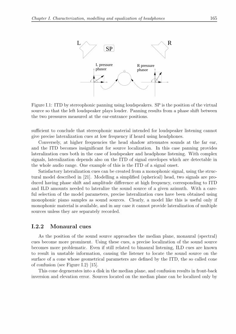
Chapter I. Characterization, modelling and equalization of headphones 165
L RSP
L pressure R pressurephasor phasor
Figure I.1: ITD by stereophonic panning using loudspeakers. SP is the position of the virtualsource so that the left loudspeaker plays louder. Panning results from a phase shift betweenthe two pressures measured at the ear-entrance positions.
sufficient to conclude that stereophonic material intended for loudspeaker listening cannotgive precise lateralization cues at low frequency if heard using headphones.
Conversely, at higher frequencies the head shadow attenuates sounds at the far ear,and the ITD becomes insignificant for source localization. In this case panning provideslateralization cues both in the case of loudspeaker and headphone listening. With complexsignals, lateralization depends also on the ITD of signal envelopes which are detectable inthe whole audio range. One example of this is the ITD of a signal onset.
Satisfactory lateralization cues can be created from a monophonic signal, using the struc-tural model described in [21]. Modelling a simplified (spherical) head, two signals are pro-duced having phase shift and amplitude difference at high frequency, corresponding to ITDand ILD amounts needed to lateralize the sound source of a given azimuth. With a care-ful selection of the model parameters, precise lateralization cues have been obtained usingmonophonic piano samples as sound sources. Clearly, a model like this is useful only ifmonophonic material is available, and in any case it cannot provide lateralization of multiplesources unless they are separately recorded.
I.2.2 Monaural cues
As the position of the sound source approaches the median plane, monaural (spectral)cues become more prominent. Using these cues, a precise localization of the sound sourcebecomes more problematic. Even if still related to binaural listening, ILD cues are knownto result in unstable information, causing the listener to locate the sound source on thesurface of a cone whose geometrical parameters are defined by the ITD, the so called coneof confusion (see Figure I.2) [15].
This cone degenerates into a disk in the median plane, and confusion results in front-backinversion and elevation error. Sources located on the median plane can be localized only by

166 Physics-based models for the acoustic representation of space in virtual environments
Median plane
R L
Figure I.2: Cones of confusion for lateralization cues given by various ITDs (far ear on theright side).
spectral cues embodied in the signal measured at the ear canal entrance. Experiments haveshown that specific bands account for different directions (without precise localization):this result is explained by the directional-band model of median-plane localization [15].Monaural cues apply only in the case that a preliminary learning process of the sound hasbeen conducted (consciously or subconsciously) by the listener, in fact they can explain thelocalization process of familiar sounds only. More in general, head movement becomes anessential mechanism in the perception of elevation, otherwise the spectral cues of the Head-Related Transfer Functions (HRTF) accounting for elevation are often barely meaningful.
For all these reasons, elevation cues are difficult to reproduce using normal equipment.Experiments on perception of elevation far from the median plane have been conductedusing normal headphones [8]. One remarkable problem lies in the fact that headphonelistening cannot account for dynamic cues, unless providing the installation with a processingsystem controlled in real-time by head tracking. Nevertheless, important interference in theexperiments comes from the listener’s awareness of wearing headphones.
Finally, an intrinsic difficulty in reproducing frontal localization would suggest that themechanisms of perceiving elevation are still not completely understood. This difficulty comesalso from the fact that binaural cues also occur during the recognition of elevation, due topinna disparity. The importance of these cues has been demonstrated by listening tests usingsubjective HRTFs individually measured at each ear: listeners, asked to rate the quality ofaudio materials in terms of elevation and IHL perception, gave the best score to recordingsplayed using individually measured HRTFs [141].

Chapter I. Characterization, modelling and equalization of headphones 167
SourceSound M M −1 Localization
Outer LocalizationEar Stage
Figure I.3: Theile’s association model. Stage labeled with M accounts for sound distortionsintroduced by the outer ear.
I.2.3 Theile’s association model
The association model of Theile (Figure I.3) gives a convincing interpretation of theunnatural colouring of sounds listened using headphones [154]. In this model it is suggestedthat distortions (denoted with M) introduced in the binaural signal by the outer ear areremoved by a canceling stage, M−1, if they are recognized for what they are, i.e. if additionalinformation coming from the external world suggests a correct positioning of the soundsource according to the acoustic information. Otherwise the stage M−1 is omitted, thusleaving unnatural color on the sound. Of course, this model is not useful in establishinglocalization models for headphone listening.
I.2.4 Other effects
IHL occurs especially because of the lost precedence effect [15], which otherwise playsa fundamental role in loudspeaker reproduction. The suppression of this effect emphasizesthe importance of a careful reverberation as perhaps the most useful strategy to externalizesounds using normal headphones. In particular, uncorrelated binaural signals obtained byproper processing of a monophonic signal have been shown to give a certain degree of out-of-head localization (OHL) during headphone listening tests [82].
In the open ear case, the ear entrance can be seen from the inner ear as a low-radiationpiston, i.e. a resistance ROE in parallel with an inductance LOE if the electrical equivalentis considered. Occluding it transforms the ear canal into a pressure chamber, turning theradiation impedance into a volume compliance or, from the equivalent electrical networkpoint of view, substituting the parallel ROE‖LOE with a capacitance CCE (see Figure I.4).This change has the noticeable effect of changing the transfer characteristic of the ear canal,producing a boost of the frequencies below approximately 2 kHz. If a carefully made head-phone tries to account for this, the occlusion effect allows bone conduction to be heard,i.e. the skull vibrations resonate in the pressure chamber. Also, occlusion can result in thetransmission to the eardrum of ultrasounds up to 100 kHz, which are heard in the form of aconstant pitch around the upper frequency limit of the hearing mechanism [11].

168 Physics-based models for the acoustic representation of space in virtual environments
CEZ
EZZ ECCEC
(a)
(b)
OEZ
EZZ ECLOER OE
Figure I.4: Occlusion effect. Equivalent circuit of the (a) open and (b) occluded ear canalseen by the inner ear. The current source accounts for signals coming to the ear-canalthrough bone conduction. The ROE‖LOE parallel becomes a capacitance CCE when the earis occluded. Impedance value at the ear canal entrance ZOE changes in ZCE. The equivalentear canal and eardrum impedances, ZEC and ZE respectively, are left unchanged.
I.2.5 Headphones vs. loudspeakers
Most of the differences between headphone and loudspeaker listening arise from the ques-tions discussed above. A well-known question lies in the so called “missing 6 dB” below 300Hz, whose explanation is quite clear for low sound pressures: sounds are masked by physio-logical noises amplified by the occlusion effect. When the sound pressure is high (typicallyabove 40 dB), the explanation is more difficult. In this case, the effect seems to depend onmechanical vibrations created by the loudspeakers, the psychological “larger acoustic size”of the loudspeaker, and possible distortions coming from amplification [131].
Under normal conditions, i.e., in a reverberant room, phase is inaudible with loudspeakerlistening. Subtle effects due to phase distortion can be heard using headphones. Thissuggests that non-minimum phase stages in the reproduction chain should be designed withparticular care, when headphones are adopted as voltage-to-pressure transducers at the endof the audio reproduction chain.
I.3 Types and modelling of headphones
The design of a high-quality headphone is a matter of experience and taste. Despite this,its main building blocks can be modelled as acoustic elements yielding pressure-flow relationsin lumped systems: volume compliances, radiating pistons, piston membranes, holes, slits.Each one of these elements has a direct counterpart in the world of electrical networks. Theelectrical equivalent circuits of the volume compliance and the radiating piston have already
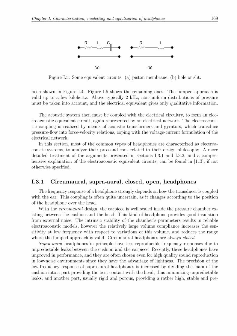
Chapter I. Characterization, modelling and equalization of headphones 169
R L C
(a) (b)
R L
Figure I.5: Some equivalent circuits: (a) piston membrane; (b) hole or slit.
been shown in Figure I.4. Figure I.5 shows the remaining ones. The lumped approach isvalid up to a few kilohertz. Above typically 2 kHz, non-uniform distributions of pressuremust be taken into account, and the electrical equivalent gives only qualitative information.
The acoustic system then must be coupled with the electrical circuitry, to form an elec-troacoustic equivalent circuit, again represented by an electrical network. The electroacous-tic coupling is realized by means of acoustic transformers and gyrators, which transducepressure-flow into force-velocity relations, coping with the voltage-current formulation of theelectrical network.
In this section, most of the common types of headphones are characterized as electroa-coustic systems, to analyze their pros and cons related to their design philosophy. A moredetailed treatment of the arguments presented in sections I.3.1 and I.3.2, and a compre-hensive explanation of the electroacoustic equivalent circuits, can be found in [113], if nototherwise specified.
I.3.1 Circumaural, supra-aural, closed, open, headphones
The frequency response of a headphone strongly depends on how the transducer is coupledwith the ear. This coupling is often quite uncertain, as it changes according to the positionof the headphone over the head.
With the circumaural design, the earpiece is well sealed inside the pressure chamber ex-isting between the cushion and the head. This kind of headphone provides good insulationfrom external noise. The intrinsic stability of the chamber’s parameters results in reliableelectroacoustic models, however the relatively large volume compliance increases the sen-sitivity at low frequency with respect to variations of this volume, and reduces the rangewhere the lumped approach is valid. Circumaural headphones are always closed.
Supra-aural headphones in principle have less reproducible frequency responses due tounpredictable leaks between the cushion and the earpiece. Recently, these headphones haveimproved in performance, and they are often chosen even for high quality sound reproductionin low-noise environments since they have the advantage of lightness. The precision of thelow-frequency response of supra-aural headphones is increased by dividing the foam of thecushion into a part providing the best contact with the head, thus minimizing unpredictableleaks, and another part, usually rigid and porous, providing a rather high, stable and pre-

170 Physics-based models for the acoustic representation of space in virtual environments
elR
0Z
nZrZ0Z
Z R
RR
L
0
L 0
R
C 1
Rod
Ear
CR 0
HR
MembraneL CMM
LRR R
RH
C 1
L M CMC 0
L0
0R
Figure I.6: Schematized isodynamic headphone (left) and its electroacoustic model (right).Particular of the electrical equivalent of the cushion in contact with the head
dictable leak. In this way the total leak Z0 (see the particular of the cushion in Figure I.6)of the acoustic chamber is represented by a parallel of two impedances, Zr and Zn, wherethe non-reproducible leak Zn has a minor effect in the equivalent impedance Z0 = Zr‖Zn.The reduced volume of the pressure chamber in the supra-aural design extends the validityof the lumped approach since standing waves appear at higher frequencies.
Supra-aural headphones can be provided with holes and/or membranes located on theexternal shell. In this case they are called open. Holes are used to gain further predictabilityof Z0. In order to counteract the contribution of the reactive component in the leak (whichincreases with frequency (see Figure I.5)), membranes can be properly placed instead of holes.Integrated open headphones with passive membranes often exhibit the most stable low-frequency response. Moreover, experiments show that more OHL localization is experiencedusing open headphones [71]. Even if some cross-talk occurs with the open design, the reasonsfor the increased OHL seem to be due to low sound reflection inside the pressure chamber,allowing a more undisturbed pinna activity, and a non-negligible perception of the externalnoise.
I.3.2 Isodynamic, dynamic, electrostatic transducers
Today, almost all high-quality headphones are provided only with isodynamic, dynamic,or electrostatic transducers, sometimes with more than one type in multi-way systems.
The isodynamic transducer consists of a large-area, low-mass surface where a conductordriven by the audio signal forms a long track covering the whole surface. A magnetic fieldperpendicular to this track is created by small magnetized rods, oriented in such a way that

Chapter I. Characterization, modelling and equalization of headphones 171
elR
Ear
L D CD
C Z M C 0Z0Z P
R 0
L 0
Z M
Z H
PZ
C
CC
CB
Z H CB
CD
DL
0C
Figure I.7: A general dynamic headphone (left) and its reduced electroacoustic model (right).
they repel each other.
The electroacoustic model accounting for circuitry, transducer and ear-coupling is given inFigure I.6 (right), together with a general scheme of the isodynamic headphone (left). Thenetwork emphasizes the presence of a resonant circuit mainly governed by the membraneparameters, CM and LM , and the volume compliance given by the pressure chamber, C0,typically producing a strong peak at around 4 kHz. This peak is damped by the resistivecomponent RR of leak ZR and, if necessary, by a porous cover over the transducer providinga further resistance RH . With this design, the leaks between cushion and head (Z0 =R0+jωL0) and the small volume compliances (C1) between the rods have far less impact thanthe main leak ZR +RH and the volume compliance C0. The large moving area, representedby the isodynamic transducer, over the relatively small pressure chamber allows extensionof the lumped approach until approximately 5 kHz. Within this band, very flat responsescan be obtained by a careful tuning of the parameters.
Dynamic headphones take advantage of the powerful pressure produced by the moving-coil transducer (approximately ten times the pressure generated by the isodynamic trans-ducer). Once again, an electroacoustic model can be developed (Figure I.7, right)1 oncethe most important elements in this design have been taken into account (Figure I.7, left).Again, the main resonance is governed by the transducer parameters, CD and LD, and thevolume compliance, C0. Resonance typically occurs at 600 Hz. The stronger sound pressurerequires a comparable damping, given by leak Z0, resistance RP within the component ZPaccounting for porous material put behind the transducer, and the resistive component ofthe impedance ZM given by passive membranes elements coupling with the pressure cham-
1the model can be reduced to the network shown here only after a first, more rigorous scheme has beencarefully studied and simplified

172 Physics-based models for the acoustic representation of space in virtual environments
−CK
−CK
0
L 0
R
Ear
C0
L M
CM
C0L0
0R
0ZCMML
KC
elR Cel
Cel
Figure I.8: Schematized electrostatic headphone (left) and its electroacoustic model (right).
ber. Non-negligible components in the computation of the low-frequency response are givenby the volume compliances existing behind the transducer, which are summarized by thecapacitance CC , the volume behind the pressure chamber (CB), and the holes necessary forthe transducer membrane to work correctly (ZH , refer also to Figure I.5).
The low-frequency response of the dynamic headphone exhibits less flatness than theisodynamic case, as damping is usually more complicated to design. The reliability of thisanalysis is also limited to a frequency of about 3 kHz. The moving coil transducer is muchmore efficient than the isodynamic one, as discussed earlier.
Electrostatic transducers (Figure I.8) are made by polarizing (typically 200 V) a mem-brane and then driving it with an electrostatic field modulated by the audio signal2. Po-larization must be kept constant. This is often produced using the power coming from theaudio signal itself, after rectification, and introducing a large resistance in series with themembrane. A drawback of this design lies in the slow re-polarization of the membrane when,during high signal levels, it touches the electrodes which form the electrostatic field, hencedischarging the capacitor. Thus, the large resistance is often spread over the membrane,thereby limiting its discharge at the contact point.
The electroacoustic model, where the acoustic transformer has been substituted by anequivalent sub-network containing two negative capacitances equal to −CK , shows that theequivalent source impedance seen by the acoustic system contains a negative reactive com-ponent. In fact, it is easy to calculate that this source impedance is equal to Rel−jωC2
K/Cel,where Cel is the capacitance of the electrodes. This reactive component has the desirableproperty of lowering the frequency peak coming from the usual resonant circuit given by thevolume compliance in series with the membrane parameters. Hence, all the considerationsmade for the isodynamic headphone design apply here, including the flat response (mainly
2typically using a push-pull circuit, to minimize distortion

Chapter I. Characterization, modelling and equalization of headphones 173
as a result of the lightness of the membrane).
The electret transducer is quite similar to the electrostatic transducer, where the mem-brane is permanently polarized.
I.3.3 Acoustic load on the ear
The acoustic load of the eardrum on the headphone, and its variations due to pressurechanges at the Eustachian tube, are recognized to have effects of low significance on theperformance of the headphone system. Conversely, experiments show that the impedancegiven by ear occlusion caused by the headphones is much more varying in frequency thanthe equivalent impedance seen by the eardrum in open ear conditions (recall the modelsshown in Figure I.4). In [163], a certain degree of correlation is shown to exist betweenthe amplitude of these variations and the quality of the equipment, the highest and mostunpredictable load being caused by some Walkman headphones under test. The increasedOHL experienced using open headphones has been already discussed in section I.2.4.
I.4 Equalization of headphones
In the previous sections we have seen the most important psychoacoustical issues relatedwith headphones, and possible ways to determine and control their low-frequency responseaccording to the type of transducer and ear coupling. It is clear that even a very carefuldesign cannot solve two important questions. First, how to decode the stereophonic materialto recreate conditions of binaural listening. Second, how to achieve a high degree of controlof the sound pressure at the ear-canal entrance, to reproduce all the cues necessary to givedefinite source localization, OHL etc.
These two questions are quite closely related. Assuming that the audio material somehowhas binaural cues encoded in it, in principle both questions would be solved by decoding andthen equalizing the audio signal, both processes now made possible by means of digital signalprocessing. In practice, and due to the not yet perfectly understood origin of many cues,the use of “transparent” headphones can make equalization much easier and effective. Thesekind of headphones have been recently made available in the form of open-canal tube-phones,although only for research purposes.
I.4.1 Stereophonic and binaural listening
In the music industry, the recording techniques are not standardized, and many aspectswhich characterize a recording session are left to the creativity of the professionals working inthat field (“Tonmeisters”). Any decoding process devoted to recovering binaural cues fromstereophonic material would in principle be ineffective, or even corrupt the quality of sound.Thus, in commercial Hi-Fi equipment stereophonic material feeds the headphones without

174 Physics-based models for the acoustic representation of space in virtual environments
passing through any special decoding process devoted to extraction of binaural cues. In thiscase stereophonic listening is performed.
On the opposite side, binaural recording must observe severe requirements. For example,it implies the use of mannequins whose heads host special in-ear microphones. Binauralrecording gives quite good results when this material is auditioned using a system for stereo-phonic listening [113]. Unfortunately, this recording technique has not achieved popularityin the studio, due to the unpredictable artifacts introduced by binaural reproduction whenthe listening conditions are not precisely determined (see section I.2.2).
Until some years ago, international standards suggested that the frequency response of aheadphone had to approximate the flat, free-field response of a loudspeaker located in front ofthe listener, i.e. the HRTF calculated in correspondence of the frontal position. This choiceoften resulted in unnatural colouring of sound, without satisfactory frontal localization (seesection I.2.2 and I.2.3). This evidence let the manufacturers design a number of alternativefrequency responses, from free-field, to diffuse field or even different characteristics [113].
I.4.2 Conditions for binaural listening
As discussed above, binaural cues cannot be easily extracted by stereophonic material.N signals xS1, . . . , xSN emitted by sources located at points S1, . . . , SN, binaurally recorded
using two microphones at positions EL and ER, are then presented to the final reproductionstage as signals xEL, xER given by∣∣∣∣ XEL(ω)
XER(ω)
∣∣∣∣ =
∣∣∣∣ HS1,EL(ω) · · · HSN,EL(ω)HS1,ER(ω) · · · HSN,ER(ω)
∣∣∣∣∣∣∣∣∣∣XS1(ω)· · ·
XSN(ω)
∣∣∣∣∣∣ (I.1)
orXE(ω) = HS,E(ω)XS(ω) (I.2)
where HSi,EP (ω) is a transfer function accounting for all the (desired and undesired, anywaysupposed linear) contributions added to the audio signal from its emission by the i-th soundsource to the final reproduction, with P = L,R.
Binaural information can be extracted from xE if the components in HS,E accounting forall the artifacts introduced by the recording and reproduction chain can be separated, i.e. ifa 2× 2 matrix MC containing all the artifacts exists such that
MC(ω)RS,E(ω) = HS,E(ω) (I.3)
RS,E containing the information about the 2×N Room Transfer Functions (RTF) calculatedfrom the sound source positions to the recording points plus the binaural cues (see FigureI.9). Headphone listening introduces new artifacts, possibly embedded in another matrix oftransfer functions calculated from the headphone input to the ear-canal entrance, writtenMH, such that the sound pressure xH measured at the ear-canal entrances obeys equation
XH(ω) = MH(ω)XE(ω) (I.4)

Chapter I. Characterization, modelling and equalization of headphones 175
ReproductionRecording
1S
S i
S N
...
...
S,ER (ω) (ω)HMMC (ω)
ER
EL
Figure I.9: Recording and reproduction of binaural material.
Binaural listening, in the form of a signal xB at the ear-canal entrances, would be realizedby post-filtering the sound material in order to compensate the artifacts coming from theaudio chain, MC, and the frequency distortions coming from headphones, MH:
XB(ω) = MH(ω)MC(ω)MH(ω)
−1XE(ω) = e−jωτRS,E(ω)XS(ω) (I.5)
where e−jωτ accounts for an overall delay coming from the compensation of non-minimumphase components [83].
The exact application of these results, i.e. a post-processing system performing a multi-channel equalization equal to C = M−1
H M−1C , is quite never realized because the knowledge of
MH is often unprecise even in the laboratory, especially at higher frequencies. Nevertheless,approximate solutions of this problem have been attempted, leading to various implementa-tions. In particular, C can be approximated as a blending stage (see Figure I.10) where thestereophonic signal is mixed to account for the interaural cues occurring during loudspeakerreproduction, otherwise lost if the same material is listened using headphones. Several typesand designs of blending circuits have been tried, from passive to active networks, even usingtubes as acoustic delay lines for the cross-talk signals, but the results obtained using theseblending architectures do not justify their systematic introduction in the reproduction chain[113].
I.4.3 Binaural listening with insert earphones
From equation (I.5), one can argue that the easier the compensation is, the higher theexpectation to reproduce the binaural signal xB. Recently, technology has made available

176 Physics-based models for the acoustic representation of space in virtual environments
C R,L
C L,R
C R,R
C L,L
R
L
Figure I.10: Block scheme of a blending circuit.
special earphones [76] which claim to have flat response at the ear-canal entrance, thiscorresponding to have |MH(ω)| ≈ I, I being the 2× 2 identity matrix. Adopting an audiochain where the response of each stage is linear3, i.e., assuming |MC(ω)| ≈ I, one canconclude that reliable conditions for a correct reproduction of binaural recorded materialnow hold.
If, in particular, the recording session is performed in an anechoic and silent environmentusing only one sound source located at a specific distance from the mannequin, then RS,E
contains the two HRTFs calculated with respect to the specific position of the sound source.In [87] these peculiar conditions have been recreated to investigate the spectral detail
needed for a precise localization of the sound source, using white noise as a test signal, xT.One key of the experiment was that the listener could not recognize whether the sound camefrom the insert earphones or from one of the loudspeakers inside the chamber, thanks to theinsert headphones. This way, the equivalence of loudspeaker and earphone reproduction hasbeen confirmed—white noise in the latter case being properly post-processed in such a waythat xB = rS,E ∗xT. Surprisingly, other valuable conclusions came out from this experiment:
1. reproduction using earphones gave good OHL as well;
2. smoothing the magnitude response in the HRTFs had no consequence until heavydistortions were introduced in the response;
3. corrupting the phase response in the HRTFs (but preserving, of course, mutual ITD),i.e., substituting the HRTFs with their minimum phase versions, did not change thelisteners’ judgement.
This test would show that OHL is perhaps the most important condition for experiencingconsistent binaural cues, and that the sensation of openness (thanks to the negligible acousticload on the ear and occlusion effect given by insert earphones) is very important to achieveOHL4. Once OHL holds, ITD and major spectral details in the HRTFs would give localization
3this assumption being quite affordable today4It must be noticed that white noise in general affords a better impression of openness. Moreover, the
sensation of openness inside an anechoic chamber is not the same one as in everyday listening conditions.
Chapter I. Characterization, modelling and equalization of headphones 177
cues, unless they are heavily corrupted.
I.5 Conclusions
The psychoacoustics of binaural listening has given a reliable starting point to investigateseveral questions left unsolved by stereophonic encoding of sound material and headphonelistening using common Hi-Fi equipment. Among the most important questions there arethe ineffective frontal localization and OHL cues provided by commercial headphones.
Localization and OHL cues can be recovered under certain conditions from binaurallyrecorded material, using special equipment which bypasses the complicate (and not yetperfectly understood) problem of how to cancel all the artifacts introduced by the recordingand reproduction chain. Head-tracking would give help in avoiding further incoherence inthe auditory messages, detected when these messages are processed by higher-level cognitivestages [57].
This kind of equipment is available only in the research laboratory at the moment. De-spite this, several results in controlled listening conditions would suggest that headphoneswill be capable of performing binaural reproductions in the near future.

178 Physics-based models for the acoustic representation of space in virtual environments

Appendix J
Computation of Linear FilterNetworks Containing Delay-FreeLoops, with an Application to theWaveguide Mesh
Federico FontanaIEEE Trans. Speech and Audio Processing.
- ACCEPTED FOR PUBLICATION -
A method that computes linear digital filter networks containing delay-free loops is pro-posed. Compared with alternative techniques existing in the literature, it does not requirea rearrangement of the network structure. Since this method involves the computation ofmatrices accounting for the connections between the filter blocks forming the network, itbecomes computationally interesting when those filters are densely interconnected throughdelay-free paths. The Triangular Waveguide Mesh is an example of such networks. Using theproposed method, we could compute a transformed version of that mesh containing delay-free loops, obtaining simulations that are significantly more accurate compared with thoseobtained using the traditional formulation of the triangular mesh.
J.1 Introduction
The delay-free loop problem [98, §6.1.3] appears during conversion to the digital domainof some analog filter networks, or during digital-to-digital domain mappings that convertunit delays into blocks that instantaneously respond to the input [81, 33]. As a consequenceof that problem, filter networks containing feedback loops may become non-computable afterthe conversion, since the computation of those loops in the discrete-time cannot be executedany longer by a sequence of operations, due to the lack of pure delays along the loop.
179

180 Physics-based models for the acoustic representation of space in virtual environments
In the case of linear filter networks delay-free loops can be detected and, then, replaced byalternative structures, to obtain equivalent, computable realizations [153]. Such replacementsusually result in changes in the original topology of the filter network.
There are cases in which a rearrangement in the filter network topology is deprecated.This happens when a filter structure cannot be merely seen as one particular realization ofa transfer function, since it contains essential information about the original system struc-ture. We deal in particular with sound synthesis using physical models: in that field, it iscommon to model spatially distributed mechanical and fluid-dynamic systems by means offilter networks that allow to inject energy and acquire responses in particular points of thesystems, along with enabling an individual control of the local parameters. The structure ofthose networks, thus, has a direct correspondence with the distribution in space of a physicalsystem [149, 13].
Recent literature pointed out that a single delay-free loop containing one linear filterin feedback can be computed without rearranging the loop structure [69]. This result hasbeen successfully applied to the computation of Warped IIR filters [70] and magnitude-complementary Tunable Equalization Filters [49].
In this paper, that approach to the delay-free loop computation has been generalized tolinear filter networks containing any configuration of delay-free loops. This generalizationyields a method that enables to detect the delay-free loops along with computing, at eachtime step, the signals that are present at any branch of the network.
In the second part of the paper, as an application case we apply the method to theTriangular Waveguide Mesh (TWM, see Figure J.1), a numerical scheme belonging to thefamily of Digital Waveguide Networks that models the ideal propagation of waves along atwo-dimensional homogeneous medium [158, 50, 13]. In that scheme, during each time step,signals incoming to a node are instantaneously scattered out into signals outgoing from thenode. As the following time step is triggered, those outgoing signals are forwarded to theadjacent nodes so that they become new incoming signals to be scattered by those nodes.
The TWM can be seen as a linear filter network in which adjacent scattering nodes areconnected one to the other via a bidirectional unitary delay line (embedded, in Figure J.1,within blocks labeled with H). With that scheme, a spectral transformation F mapping eachunit delay into a corresponding first-order allpass transfer function A, i.e., the followingtransformation of the z-variable [98]:
z−1 = F−1(z) = A(z) =z−1 − λ1− λz−1
, (J.1)
has been shown to have considerable benefits in the accuracy of the results provided by themodel, once the allpass coefficient λ is properly set [137].
The proposed method allows to compute the signal in the TWM after the network hasbeen transformed using (J.1). Responses coming from the “warped” version of the TWM,from here called warped TWM, are presented in the conclusion of the paper.

Chapter J. Computation of Linear Filter Networks Containing Delay-Free Loops, with anApplication to the Waveguide Mesh 181
H H H H
H
H H H
H
H H H H
H
H
H H H
H
H H H H
H H H H
H H
H H H
H H H H
H H HH
H
H
H
H
H
H
H
H
H
x
z −1
z −1
Figure J.1: Triangular Waveguide Mesh. Adjacent nodes are connected each other via bidi-rectional unitary delay lines (embedded within the blocks labeled with H, see particular), thatreceive/inject signals from/to the nodes, respectively. Signals are instantaneously scatteredby each node.
J.2 Computation of the Delay-Free Loop
First, we briefly revise the method proposed by Harma [69] for computing a single delay-free loop in the form expressed by the upper structure in Figure J.2, where x and y arerespectively the input and output signals, and it is
H(z) =
b+M∑k=1
bkz−k
1−N∑k=1
akz−k
. (J.2)
The method considers, at any discrete-time step n, the output o from the feedback branch asa linear superposition of two components: the former accounts for the instantaneous reactionof the filter in feedback; the latter, q, depends on its internal state. Thus, by (J.2), it iso[n] = by[n] + q[n]. Hence, the output from the delay-free structure can be written as
y[n] = x[n] + o[n] = x[n] + by[n] + q[n] , (J.3)

182 Physics-based models for the acoustic representation of space in virtual environments
+
H(z)
x
o
y
+
H(z)
+x
q b
y
Figure J.2: Delay-free loop structure (above). Rearrangement of the delay-free loop structureaccording to the procedure proposed in Section J.2 (below).
which implies
y[n] =1
1− b
x[n] + q[n]
. (J.4)
This algebraical rearrangement of the delay-free loop can be always done, even for un-stable structures, except for cases in which it is b = 1. In those cases it can be demonstratedthat the structure is non-causal, since its input/output transfer function has a singularity inthe infinite point of the z-plane [69].
Since q can be computed at any time step by feeding the filter with a null sample, thenthe output from the structure can be computed by means of a procedure that makes use ofthree steps, which are executed at each n (see the lower part of Figure J.2):
1. q is computed feeding the feedback filter with zero;
2. y is computed using (J.4);
3. y is fed to the filter in feedback, to update its state correctly.
J.3 Computation of Delay-Free Loop Networks
Any procedure leading to the computation of the delay-free loop must, in a way oranother, rearrange the non-computable structure. The procedure proposed in Section J.2isolates a sub-loop that accounts for the instantaneous part of the response of the feedbackfilter (see Figure J.2). That idea is now generalized to linear filter networks containingmultiple delay-free loops.
Suppose to isolate, from the filter network, a number of subnetworks containing delay-freeloops. In order to do this we can take advantage from a graph-theoretic detection methodexisting in the literature [153]. We now treat each subnetwork separately.

Chapter J. Computation of Linear Filter Networks Containing Delay-Free Loops, with anApplication to the Waveguide Mesh 183
++
yi1
yiPi
+ ix
u i
(z)H iq i
iyib
Figure J.3: Structure of a filter branch. The output yi is obtained as a superposition of onecomponent depending on the input xi, plus one input-independent component qi. The inputis the result of summing outputs yi1 , . . . yiPi from other branches plus one external input ui.
Let us index each one of the L filter branches forming a subnetwork. Each branch providesthe transfer function
Hi(z) =
Mi∑k=0
bk(i)z−k
1−Ni∑k=1
ak(i)z−k
, i = 1, . . . , L . (J.5)
Similarly to what we have seen in Section J.2, for each one of those branches we isolate, inthe output yi, the addendum containing the instantaneous input xi. Hence, for the i-th filterbranch we can write
yi[n] = bixi[n] + qi[n] , (J.6)
where clearly it is bi = b0(i). Note that bi is non null, since the subnetwork resulting after the
application of the delay-free loop detection method cannot contain branches correspondingto pure delays. On the other hand, qi can be null at any time step when the filter in thei-th branch reduces to a multiplier. In particular, we can account for direct connections, i.e.,yi = xi: they will be represented by branches where it is bi = 1 and qi ≡ 0.
Now, we consider the inputs to any filter branch. Each input xi is the superposition ofPi outputs yi1 , . . . yiPi from other branches plus an external input ui, null if the filter branchis fed only by outputs from other branches (see Figure J.3):
xi[n] =
Pi∑k=1
yik [n] + ui[n] . (J.7)
Note that direct loopbacks connecting yi and xi are avoided. In other words, condition
ik 6= i , k = 1, . . . , Pi (J.8)
must be satisfied for any i. For this purpose, each direct loopback is indexed in the subnet-work separately, in a way that its index respects condition (J.8).

184 Physics-based models for the acoustic representation of space in virtual environments
By collecting the outputs y1, . . . , yL together in the column vector y, and doing the samealso for x, q and u, (J.6) and (J.7) can be expressed by the following vectorial equations,respectively:
y[n] = Bx[n] + q[n] (J.9a)
x[n] = Py[n] + u[n] (J.9b)
where B is a non-singular matrix containing the coefficients b1, . . . , bL in its diagonal andzero elsewhere, and P is a matrix accounting for the connections among branches. Elementpij of P is equal to one if the output of the j-th filter branch feeds the i-th filter, otherwiseit is equal to zero. The exclusion of direct loopbacks in the network, expressed by (J.8),constrains the diagonal of this matrix to be null.
Substituting (J.9b) in (J.9a), after the elimination of x, we find a way to calculate thefilter outputs from values that are independent of the delay-free loops:
Fyy[n] = Bu[n] + q[n] , (J.10)
with Fy = I −BP =
=
1 −b1p12 ... −b1p1L
...
... 1...
...
−bLpL1 ... −bLpLL−1 1
, (J.11)
I being the L×L identity matrix. Each element ij of Fy contains the i-th diagonal elementof B changed in sign, gated by the element ij of P .
The existence of the inverse matrix Fy−1 determines whether the output y can be calcu-
lated or not. Here we show that if the inverse matrix does not exist, then the subnetworkupon consideration contains non-causal loops. In fact, after formal substitution of y, uand q with their corresponding z-transforms, respectively Y , U and Q, then (J.10) can beexpressed in the z-domain:
FyY (z) = BU(z) +Q(z) , (J.12)
such that
Y (z) =adjFydetFy
BU(z) +Q(z)
(J.13)

Chapter J. Computation of Linear Filter Networks Containing Delay-Free Loops, with anApplication to the Waveguide Mesh 185
where the operator adj gives the adjoint matrix.In the hypothesis that the input signal is causal and bounded, and the initial energy in
the network is finite (that is, |q[0]| < ∞), then, recalling a known theoretical result [110,§4.4.8], we have
limz→∞
Y (z) =adjFydetFy
Bu[0] + q[0]
. (J.14)
This limit is equal to infinity for some scalar functions Yi(z), i = 1, . . . , L, as long as detFygoes to zero and it is Bu[0]+q[0] 6= 0. Hence, if Fy is singular then the subnetwork containsnon-causal loops.
In the case when it is u ≡ 0 and q ≡ 0 during the whole process, the limit (J.14) cannotbe determined when Fy is singular. This case includes pathological situations. For instance,consider the delay-free loop of Figure J.2, where the loopback filter is a pure multiplier (thatis, q ≡ 0), in a way that the upper and lower structures match each other. Let us set b = 1and u = 0 at time step n. In principle, the loop will keep on producing an output that isconstantly equal to y[n − 1] as long as u is null. Otherwise, i.e., for b = 1 and u 6= 0, theoutput cannot be calculated.
On the other hand, stability is not necessarily required for the existence of Fy−1. The
inverse matrix allows to calculate the output explicitly:
y[n] = Fy−1Bu[n] + Fy
−1q[n] . (J.15)
In summary, at each time step the procedure that computes the subnetwork containingdelay-free loops is the following:
1. compute q[n], feeding each filter branch with zero;
2. compute y[n] from (J.15);
3. compute x[n] from (J.9b);
4. feed the filters in the subnetwork with x[n] to update their state.
Symmetrically, another procedure can be executed. In fact, Equation (J.9a) can besubstituted in (J.9b) in such a way that, after the elimination of y, an explicit solution isfound out for x[n] rather than y[n]:
x[n] = Fx−1Pq[n] + Fx
−1u[n] , (J.16)
withFx = I − PB . (J.17)
Equation (J.16) can be solved if and only if (J.15) admits solution (see Appendix).Hence, a symmetric procedure can be devised:
1. compute q[n], feeding each filter branch with zero;

186 Physics-based models for the acoustic representation of space in virtual environments
2. compute x[n] from (J.16);
3. compute y[n] from (J.9a);
4. feed the filters in the subnetwork with x[n] to update their state.
Finally, it is worth mentioning that the method works also in the case whenB is singular,that is, when some filter branches in the subnetwork do not respond instantaneously to theinput. In other words, filter branches characterized by having bi = 0 can be included in thesubnetwork without harming the procedure. This is proved in the Appendix.
The possibility to extend the given method to any linear filter network is useful, forexample, if the filter coefficients are varied runtime, since it prevents the procedure to failas long as bi is set to zero at some branches during the computation.
J.3.1 Detection of Delay-Free Loops
The extension to cases in which it is bi = 0 for some branches enables the method todetect the delay-free loops that are present in a filter network. To show this, first we givea rule for deciding which filter branches are part of a delay-free loop. The decision is takenchecking the two following conditions for any pair (i, j) of filter branches. Thus, two branchesi and j are part of the same delay-free loop if
1. a variation of qj generates a perturbation in yi instantaneously, and
2. a variation of qi generates a perturbation in yj instantaneously,
otherwise those branches are not part of the same delay-free loop.
Note that the rule holds also in the case when qi ≡ 0 and/or qj ≡ 0, i.e., if branchescorresponding to pure multipliers are involved in the decision. In that case, an equivalentvariation occurring at the same point where qi and/or qj is injected into the loop (refer toFigure J.3) can be considered instead.
The two statements can be checked automatically once Fy−1 is known. In fact, it can be
seen from (J.15) that this matrix puts the filter outputs in relation with the state vector, insuch a way that the verification of the two statements corresponds to checking that
(Fy−1)ij 6= 0 , (Fy
−1)ji 6= 0 (J.18)
where (·)ij is the element ij of a matrix. In other words, two branches i and j are part of thesame delay-free loop if and only if the element ij of Fy
−1 and its transposed are not null.
In the Appendix, a delay-free loop network proposed by Szczupak and Mitra [153, exam-ple 2] is resolved using the detection method proposed here.

Chapter J. Computation of Linear Filter Networks Containing Delay-Free Loops, with anApplication to the Waveguide Mesh 187
J.4 Scope and Complexity of the Proposed Method
The proposed method involves the definition of a linear system from each subnetworkcontaining delay-free loops, whose dimension equals the number of filter branches existing inthe subnetwork. The solution of that system provides formulas, (J.15) or (J.16), that yieldthe output y or input x, respectively. We cannot avoid the matrix calculations contained in(J.15) or (J.16), since any state variation and/or any new external input occurring somewherein the subnetwork produce global effects on it in the form of output variations at all the filterbranches composing the subnetwork, except for those that do not respond instantaneouslyto an input (for which the method is useless).
Although digital signal processors are usually well-suited to perform sequential matrixcomputation, and given that the computation of (J.15) or (J.16) can be parallelized, forexample over L processors, yet the key feature of the method is the definition of a procedurethat allows to calculate not only the output from the subnetwork, but also its internal signals.
Nevertheless, its computational performance can be interesting in the case of “dense”networks, that is, networks where each filter block feeds most of the other filters. In thelimit case when each branch feeds all the other branches, and assuming that all filters in thenetwork are N -th order filters, each one provided with an external input, then we have fromEqs. (J.7) and (J.5):
Yi(z) = Hi(z)Xi(z) = Hi(z)
L∑k=1k 6=i
Yk(z) + Ui(z)
, (J.19)
i = 1, . . . , L .
Equation (J.19) can be expressed in matrix form,
H−(z)Y (z) = U (z) , (J.20)
with
H−(z) =
1H1−1 −1 . . . −1
−1 1H2−1 . . . −1
.... . .
...
−1 . . . −1 1HL−1
−1
−1 . . . −1 −1 1HL
. (J.21)
Assuming that the inverse of H− exists, then we have
Y (z) = H−(z)−1U (z) =adjH−(z)
detH−(z)U (z) . (J.22)

188 Physics-based models for the acoustic representation of space in virtual environments
+F −1x
y1
yL
H
H
1
L
u
P
1 1
L L
x
x
q
q
Figure J.4: Schematic of the latter procedure given in Section J.3. Individual filter blocksare in transposed direct form.
Equation (J.22) shows that in the limit case hypothesized here the extraction of all thefilter outputs, using a traditional method that rearranges delay-free loops into an alternativenetwork, involves in principle the computation of L2 filters having order LN , each one repre-sented by one element of H−(z)−1. In other words, the computation of a dense filter networkcontaining delay-free loops turns into an algorithm that, without a peculiar reformulation ofthe structure that computes H−(z)−1, in general has a complexity O(NL3).
Compared to that, the proposed method needs:
• 4(L − 1)2 operations to compute (J.15) or (J.16)—step 2 of both procedures given inSection J.3;
• 2(L − 1)2 + L operations to compute x from (J.9b) or y from (J.9a)—step 3 of thesame procedures;
• another order of LN operations to compute q and to update the state of the L filters—steps 1 and 4.
Then, the algorithm coming from the proposed method has a complexity O(NL2).In the case when the filters H1, . . . , HL can be realized in transposed direct form, then q
can be directly read from the filter states so that step 1 is skipped. A schematic of the latterprocedure given in Section J.3 is shown in Figure J.4, where the individual filter blocks havebeen realized in transposed direct form so that they yield q directly.
In most of the potential application cases Fy and Fx are sparse matrices, since the filteroutputs feed only a small part of the inputs belonging to other filter branches. In thosecases, efficient inversion procedures can be invoked [65] if Fy
−1 or Fx−1 must be recomputed
runtime, for example when the filter coefficients are varied. Although traditional delay-free

Chapter J. Computation of Linear Filter Networks Containing Delay-Free Loops, with anApplication to the Waveguide Mesh 189
loop computation methods seem to cope more effectively with those cases, especially in real-time applications, it should be noted that rearrangements in the filter network, that areneeded by those methods to remove the delay-free loops, usually lead to structures wherethe filter coefficients are no longer directly tunable.
J.5 Application to the TWM
TWMs define stable, energy-preserving filter networks, whose structures have a directcorrespondence with the geometry of an ideal elastic membrane [13]. The scattering nodeshave also the function of input/output points, so that they form a discrete set of locationswhere the (position-dependent) transfer functions measured from one input point to oneoutput point of the membrane can be computed from the model (see Figure J.1).
Waveguide Mesh models introduce, in the simulations, a numerical error called dispersion[152, 158]. In the case when a TWM is used to model a membrane, then dispersion can beequivalently interpreted, with good approximation, as a frequency-dependent change in prop-agation speed of the waves that resonate in the system, causing a proportional misplacementof the modal frequencies in the model response. This change in speed is quantified by the dis-persion function D, that yields the propagation speed ratio between modeled (“dispersed”)and ideal (“undispersed”) traveling wave components. The dispersion function decreaseswith frequency, suggesting that high frequency waves are affected by a larger propagationspeed error [50].
A manipulation of the wave propagation speed would have benefits in the accuracy ofthe simulations provided by the TWM. This manipulation can be done by transforming eachpure delay into a frequency-dependent phase shift, in a way that the new blocks obtainedafter that transformation reduce the error caused by dispersion. In practice, these blocksintroduce a specific phase delay to any frequency component as long as it is transferred fromone scattering node to another.
Allpass-to-allpass transformations may provide that kind of manipulation if their pa-rameters are properly set, meanwhile they preserve the properties of stability and energypreservation of the TWM. The spectral transformation F given by (J.1) has been shownto improve the model accuracy significantly [137]. Previous literature proposed frequencywarping as a technique for computing off-line the TWM as if it were transformed by F , alongwith a strategy for optimizing the λ coefficient over a limited part of the spectrum [137].We exploit the method introduced in Section J.3 to compute the transformed TWM online,optimizing λ over the entire spectrum.
The following instantaneous scattering equation holds for any internal node of a TWM

190 Physics-based models for the acoustic representation of space in virtual environments
[150]: ∣∣∣∣∣∣∣∣∣∣∣∣
xA−
xB−
xC−
xD−
xE−
xF−
∣∣∣∣∣∣∣∣∣∣∣∣=
−23
13
13
13
13
13
13
−23
13
13
13
13
13
13
−23
13
13
13
13
13
13
−23
13
13
13
13
13
13
−23
13
13
13
13
13
13
−23
∣∣∣∣∣∣∣∣∣∣∣∣
yA+
yB+
yC+
yD+
yE+
yF+
∣∣∣∣∣∣∣∣∣∣∣∣(J.23)
where A+, . . . , F+ and A−, . . . , F− index the branches incoming to and outgoing from theinternal scattering node, respectively.
The nodes forming the boundary reverse the sign of any incoming wave signal, given thatthe TWM simulates a membrane ideally clamped at the border:
xG− = −yG+ , (J.24)
where G+ and G− are indexes of filter branches incoming to and outgoing from the boundarynode, respectively.
Relations (J.23) and (J.24) are used to form the matrix P , that, hence, has the aspectof a sparse matrix: elements accounting for boundary reflections are equal to −1; elementsaccounting for internal wave reflections are equal to −2/3; finally, elements accounting forinternal wave transmissions from one branch to another are equal to 1/3. Note that a rigorousapplication of the method, i.e., the definition of a matrix P containing only elements equalto either zero or one, would have required to define a larger number of filter branches withno advantages in the implementation of the model.
The output signal v from a node can be computed, at each time step, doubling theaverage of either its incoming or outgoing wave signals:
v =1
3yA+ + . . .+ yF+ =
1
3xA− + . . .+ xF− . (J.25)
from (J.1) it is B = −λI. From (J.11) and (J.17) we have Fy = Fx = I + λP . Fy−1 and
Fx−1 do not contain null elements, suggesting that the warped TWM is made of one delay-
free loop as a whole, where a variation occurring at any filter branch induces perturbationsover the whole rest of the mesh. This behavior must not lead the reader to the conclusionthat wave signals in the warped TWM propagate at infinite speed along the mesh. Rather,it can be seen as an effect of the finite bandwidth of the discretized wavefronts propagatingalong the warped TWM.
If the allpass filters reduce to pure delays (λ = 0), nevertheless the computing procedurekeeps on working as explained at the end of Section J.3. Under this condition it is B = 0,and Fy = Fx = I. In that case it can be easily seen that, during the free evolution of thesystem, both procedures given in Section J.3 reproduce exactly the computations that arerequired to simulate the free evolution of the original TWM [158, 50].

Chapter J. Computation of Linear Filter Networks Containing Delay-Free Loops, with anApplication to the Waveguide Mesh 191
J.5.1 Reducing dispersion
Dispersion can be exactly calculated for any (two-dimensional) spatial frequency compo-nent traveling along the mesh [152, 13]. In polar coordinates, dispersion can be seen as afunction of direction θ and magnitude ξ of the spatial frequencies, D(θ, ξ).
In the TWM, traveling wave components propagate with a speed error that is, with goodapproximation, independent of the direction of propagation [137]. For this reason, dispersioncan be averaged into a single-variable function D(ξ) that, although depending only on thefrequency magnitude, still provides information with sufficient precision:
D(ξ) =1
2π
∫ 2π
0
D(θ, ξ)dθ =2
π
∫ π/2
0
D(θ, ξ)dθ . (J.26)
This averaging can be safely done up to the edge of the spatial bandwidth, that is equal toξMAX = 1/(d
√3) in the case of a TWM whose scattering nodes are separated by a distance
d, corresponding to the waveguide length [53].Recalling the nominal (undispersed) wave propagation speed in a two-dimensional waveg-
uide mesh [158]
c =1√2dFs , (J.27)
where Fs is the sampling frequency, then from D(ξ) we can calculate the misplacementaffecting a resonance frequency f . In fact, that resonance comes from a standing wavehaving spatial frequency magnitude ξ = f/c, in a way that the dispersion ratio for thatresonance is equal to:
f
f= D(
f
c) = D(
f√
2
dFs) , (J.28)
where f is the frequency of the misplaced resonance. This formula is valid over a frequencydomain limited by
fMAX = cξMAX =1√2dFs
1
d√
3=
Fs√2√
3<Fs2
. (J.29)
Above this limit (that lies below the Nyquist limit, as emphasized also in (J.29)) the TWMdoes not generate resonances1.
From (J.28) we can immediately figure out a function D, mapping undispersed intodispersed frequencies:
f = D(f) = fD(f
c) . (J.30)
1More precisely, the TWM can process two-dimensional signals having spectral components up to ξ =2/(3d), that is, recalling (J.29), the temporal frequency domain is absolutely limited by 2c/(3d) = Fs
√2/3 ≈
0.471Fs. Such components exist only for certain directions θ [53]: for this reason, the spatial band rangingfrom ξMAX to 2/(3d) cannot be part of the domain of D(ξ), although resonances located at frequencies thatare higher than fMAX appear in the impulse response of a TWM.
192 Physics-based models for the acoustic representation of space in virtual environments
On the other hand, the transformation (J.1) induces the following mapping between thedomain of the untransformed (i.e., misplaced) resonances f and the transformed (or warped)frequencies f [101]:
f = F(f) =Fs2π
arctan(1− λ2) sin(2πf/Fs)
2λ+ (1 + λ2) cos(2πf/Fs)(J.31)
where it is z = ei2πf/Fs . In particular, the derivative calculated at dc of (J.31) is equal to
F0 =F(f)
′f=0
=1− λ1 + λ
. (J.32)
Equation (J.32) gives reason of the fact that dispersion is reduced by the allpass map (J.1)at the cost of an overall phase delay change (also called warping ratio in the literature) that,for positive values of λ, shrinks the frequency response by a factor F0 [137]. This correspondsto reducing the wave propagation speed in the TWM by the same factor.
Summarizing, in the warped TWM the frequency domain is transformed by two maps,the former caused by dispersion, the latter induced by the allpass transformation:
fD−→ f
F−→ f , (J.33)
such that
f = FD(f) , 0 ≤ f < fMAX (J.34)
An optimal value for λ can be found, for instance, minimizing the distance between f and fover the domain where the TWM produces resonances, independently of the warping ratioF0:
minλ:|λ|<1
∣∣∣∣∣∣ fF0
− f∣∣∣∣∣∣
2, 0 ≤ f < fMAX . (J.35)
We have computed (J.26), (J.34) and (J.35) numerically, assuming as a metric for distancethe L2 norm of a real sequence s, i.e., ||s||2 =
∑l s
2[l]. The above minimization yieldsλ = 0.2200, and, consequently, F0 = 0.6393. Figure J.5 shows (in normalized frequencyscales) plots of both maps, D and F (the latter divided by F0 to hide domain shrinking),together with their composition using the optimal value λ.
J.5.2 Results
Figure J.6 shows the frequency response coming from a TWM model, sampled at 8 kHz,of a square membrane sized 0.3 m, with waves traveling at a speed equal to 131 m/s. Thosequantities define a TWM having size equal to 13 waveguides (numbering them along one ofthe waveguide orientations, such as x in Figure J.1). Together with the plot of the response,the positions of the theoretical modes resonating in that membrane below fMAX are depicted

Chapter J. Computation of Linear Filter Networks Containing Delay-Free Loops, with anApplication to the Waveguide Mesh 193
0 0.1 0.2 0.3 0.4 0.50
0.1
0.2
0.3
0.4
0.5
Normalized frequency (Hz)
Nor
mal
ized
freq
uenc
y (H
z)
identity mapallpass mapcompositiondispersion
Figure J.5: Normalized frequency domain mappings induced by the warped TWM (solidlines) plus identity map to be taken as reference (dashed line). Referring to the right endof each plot: dispersion function D (bottom); allpass map F/F0 with λ = 0.2200 (top);composition of the two (middle).
with ‘’ (without dispersion) and ‘+’ (after dispersion), respectively. The correspondencebetween theory and simulation is good.
Some interesting considerations emerge from the analysis of that response. Since theexcitation and the acquisition points are located close to the boundary, the lowest resonances(in particular the first one, called the fundamental) have a smaller magnitude. Moreover,the magnitude response drops down above fMAX, i.e., above the frequency labeled by theupmost ‘+’ symbol2.
This TWM is made of 998 waveguide branches. Thus, the computation of the corre-sponding warped TWM involves matrices having identical dimension. Figure J.7 showsfigures taken from that warped TWM, assuming λ = 0.2200. The matching between theo-retical resonance positions (depicted with ‘+’), calculated for the warped model using (J.34),and corresponding peak positions in the warped TWM response is satisfactory. Moreover,the theoretical modes produced by the original square membrane below fMAX have beenpresented once more, using ‘’ symbols, after their positions have been divided by F0 toaccount for the proportional wave speed reduction caused by the allpass transformation.
Alternative minimizations can be chosen instead of (J.35), for instance operating oncertain bands such as the low frequency [137]. Moreover, higher order allpass-to-allpasstransformations can be taken into consideration: although resulting in more accurate phase
2As briefly explained in footnote 1, this happens because only a few, direction-dependent waves canresonate in the TWM beyond that frequency.

194 Physics-based models for the acoustic representation of space in virtual environments
0 500 1000 1500 2000 2500 3000 3500 4000−30
−20
−10
0
10
20
30
Frequency (Hz)
Gai
n (d
B)
TWMtheoretical res.dispersed res.
Figure J.6: Frequency response (Fs = 8 kHz) of a TWM modeling a square membrane sized0.3 m; waves traveling at c = 131 m/s. Resonance positions of the membrane below fMAX
(‘’). Dispersed resonance positions of the membrane below fMAX (‘+’).
equalizations, meanwhile they might excessively distort the overall frequency response. As astarting point, the warping ratio can be used as a prior figure for the analysis of the overalldistortion caused by a transformation.
The proposed method can be used in alternative configurations of Digital Waveguide Net-works, whenever an improvement in the accuracy of the simulations justifies its application[51, 138, 13].
J.6 Conclusion
A method for the detection and computation of delay-free loops in linear filter networkshas been proposed. That method translates automatically into a procedure that detectsthe delay-free loops and computes such networks. Compared with traditional methods, theefficiency of the computation becomes interesting in the case of dense filter networks, as longas their branches process signals that must be presented at the system output.
The proposed method turns out to be useful in the simulation of distributed systems, suchas Digital Waveguide Networks, when they implement delay-free transmission in consequenceof the application of spectral mappings that eliminate pure delays. As an application casewe have computed a warped Triangular Waveguide Mesh, that has been shown to providemore accurate simulations compared with the traditional triangular mesh.

Chapter J. Computation of Linear Filter Networks Containing Delay-Free Loops, with anApplication to the Waveguide Mesh 195
0 500 1000 1500 2000 2500 3000 3500 4000−30
−20
−10
0
10
20
30
Frequency (Hz)
Gai
n (d
B)
wTWMtheoretical res.warped res.
Figure J.7: Frequency response (Fs = 8 kHz) of a warped TWM (λ = 0.2200) modeling asquare membrane sized 0.3 m; waves traveling at c = 131 m/s. Resonance positions of themembrane below fMAX corrected by factor F0 = 0.6393 (‘’). Calculated resonance positionsfor the warped TWM (‘+’).
Acknowledgments
The Author is grateful to Dr. Aki Harma for his insightful and patient feedback, toProf. Davide Rocchesso, who helped with several suggestions, and to Prof. Matti Karjalainen,who contributed to inspire this research.
J.7 Appendix
J.7.1 Existence of the solutions
Recalling that B is full-rank, it is
detFx = det(I − PB) = det(B−1 − P ) det(B) (J.36)
= det(B) det(B−1 − P ) = det(I −BP ) = detFy .

196 Physics-based models for the acoustic representation of space in virtual environments
12
34
6
7
89
10
1314
15
12
11
5
Figure J.8: Connected graph (taken from Szczupak and Mitra, ordering branches instead ofnodes).
J.7.2 Extension of the method to any linear filter network
Let bi = 0 for the i-th filter branch. Recalling (J.11), this means that the i-th row of Fyis null except for the i-th element, that is equal to one. Hence, we have that
detFy = (detFy)i , (J.37)
where (detFy)i is the minor determinant resulting from the removal of the i-th row andcolumn from detFy. By (J.36), this means that Eqs. (J.15) and (J.16) admit solution inparticular when it is bi = 0.
Relation (J.37) can be repeatedly applied to all the branches, say i1, . . . , iR, such thatbi1 = . . . = biR = 0:
detFy = (. . . (((detFy)i1)i2) . . .)iR . (J.38)
Hence, the proposed procedure for the computation of the delay-free loop can be extendedto any linear filter network.
J.7.3 Detection of delay-free loops
The graph proposed by Szczupak and Mitra is repeated in Figure J.8 except for thetype of ordering, involving branches instead of nodes [153]. Holding the hypothesis that it

Chapter J. Computation of Linear Filter Networks Containing Delay-Free Loops, with anApplication to the Waveguide Mesh 197
represents a causal filter network (this is true, i.e., detFy 6= 0, if, for instance, it is bi = i),then Fy
−1 has the structure below:
1 2 3 4 5 6 7 8 9 10 11 12 13 14 15
1 • • • • • • • • • • • • • • •
2 • • • • • • • • • • • • • • •
3 • • • • • • • • • • • • • • •
4 • • • • • • • • • • • • • • •
5 • • • • • • • • • • • • • • •
6 • • • • • • • • • • • • • • •
7 • • • • • • • • • • • • • • •
8 •
9 • • •
10 • • • • • • • • • • • • • • •
11 • • • • • • • • • • • • • • •
12 • • • • • • • • • • • • • • •
13 • • • • • • • • • • • • • • •
14 • • •
15 •
where non-zero elements have been represented using the symbols ‘•’ and ‘’, whereas nullelements have been left blank. From that structure, using the rules given in Section J.3.1, itcan be concluded that:
• branches 1-7 and 10-13 are part of the same delay-free loop (elements depicted with‘•’);
• branches 8 and 15 form a separate delay-free loop (elements depicted with ‘’);
• branches 9 and 14 do not belong to any delay-free loop (in fact they form the orientedcut set, alternatively figured out by Szczupak and Mitra [153]).

198 Physics-based models for the acoustic representation of space in virtual environments

Appendix K
Acoustic distance for scenerepresentation
Federico Fontana, Davide Rocchesso and Laura OttavianiIEEE Computer Graphics & Applications.
- SUBMITTED FOR REVIEW -
There are cases in which not all the objects and events forming the scene can be visuallyrepresented simultaneously. In those cases the scene representation can be complementedby the acoustic mode. Here we show that sounds representing objects and events in thedisplay can be manipulated so to inform the user about her relative distance from thoseobjects. We do this by simulating the everyday-listening experience, during which we getauditory cues from sound sources located at different relative distances from us. This kindof manipulation neither changes the nature of the sound source nor interferes with the visualinformation, hence its use produces an absolute increase of the bandwidth of interaction in themultimodal display. Limits in the adoption of the proposed technique come by unavoidableblurs exhibited by humans in estimating distance using the auditory system. On the otherhand, representing range data through the virtual reconstruction of auditory distance cuesrequires neither previous training or learning effort for the user, nor the adoption of specificaudio virtual reality reproduction systems.
K.1 Introduction
The representation of a virtual scene, provided to a user by a computer interface, takesadvantage from the existence of information channels alternative to the visual one. Althoughthe video plays a major role in the presentation of virtual scenarios, nevertheless the acousticmodality, in the form of speech and also non-speech output, increases the user’s engagementand, provided that the audio message is correctly displayed, can enlarge the bandwidth ofinteraction in a multimodal display.
199

200 Physics-based models for the acoustic representation of space in virtual environments
Improving the interactivity in a virtual environment by adding auditory information atthe interface output is not straightforward, especially when non-speech communication isconsidered. In fact, the mere addition of sound in the display, regardless of which soundsto play, and how to display them, may result in the opposite effect, diminishing the user’sperformance, engagement and satisfaction.
Rather, the auditory mode requires to be correctly integrated with the rest of the display.An effective integration needs the solution of several issues of sonification and spatialization(see Sidebar 1). In the end, the user should experience a virtual environment where soundsaugment the realism, providing messages that integrate the visual information and sometimessubstitute it, for example when an object has been visually occluded by other elementsappearing in the visual scene, or when the user is visually impaired so that her perceptionof a scenario strongly or completely relies on non-visual information [84].
In our research we deal with the representation of the distance in a user-centered (typically3-D) virtual scenario. In principle the question is trivial: most of the objects appearing ina scene are recognized for what they are through the visual information displayed at theinterface, in a way that their distance is estimated, with some approximation, as part of thisinformation. Nevertheless, there are cases in which a multimodal, audio-visual representationof distance turns out to be useful. Given that the object/user distance emerges as an essentialinformation in the display, those cases include (see also Figure K.1):
• objects that fall out of the visual angle. This is the case of large screens;
• objects whose relative distance the user must continuously survey, even during tasks inwhich the focus of visual attention is somewhere else. This happens especially duringcritical tasks, which prevent the user to steer the visual attention;
• objects outside the visual display. This can occur in the case of small screens;
• objects popping up somewhere, as new elements in the scene, whose existence must berapidly declared to the user;
• objects whose relative distance can be hardly estimated by vision, unless the user startssome action such as navigating in the scene to get more information about the object:changing her viewpoint, for example, or looking for landmarks which help figuring outthe object position and, hence, its relative distance. This situation can take placein virtual scenarios where the use of stereoscopic vision is not enabled, when objectswhich are unfamiliar to the user’s eye are displayed.
In all the above cases, supporting the visual rendering model with a tool for the real-timesynthesis of auditory distance cues can lead to advantages in the display quality, concerningthe representation of the distance of objects.

Chapter K. Acoustic distance for scene representation 201
?
??
Figure K.1: Visual displays have their own limits. Objects and/or events located outside thevisual angle, outside the screen, and objects which are out of the focus of visual attentionwould be conveniently displayed using another modality.
K.2 Hearing distance
We want to put the user in condition to perceive distances, by integrating non-speech au-dio communication at the interface output. In principle, such a choice is prone to objections.In fact, even in the contexts pointed out in Section K.1 we can find alternative solutions,making use of either the visual or auditory mode.
Solutions using the visual mode may be provided, for example, by sidebars containingrange indicators. In the case when the visual attention should focus on a single task, thendigits informing about the distance of objects located somewhere else might be added in thevisual display. Those digits should be visualized close to the position in the display where thetask takes place, or they could be superimposed, in the same position, as semi-transparentlayered images.
The same information can be conveyed through the auditory mode, for example using asynthetic voice that tells the range to the user through periodic vocal messages or, alterna-tively, using non-speech sonification strategies.
Although methods which exploit either the visual or auditory mode can be worked outeffectively, even leading to a precise presentation of data, nevertheless a conventional displaymethod for presenting distance, such as those which we have just described, will probablylead to machine-to-user communication streams which saturate a non-negligible (and possiblyprecious) portion of the overall available bandwidth of the visual or auditory informationchannel, respectively.

202 Physics-based models for the acoustic representation of space in virtual environments
We will show that a less conventional method can be found, for presenting the data insuch a way that they fill a band of the auditory channel which is, to a wide extent, disjoinedfrom the portion normally occupied by speech and non-speech audio communication streams.Such a band exploits a perceptual dimension that has been hardly ever considered interestingfor data communication. More precisely, we are going to integrate distance in the form ofan auditory spatial cue to existing speech or sonic messages, in a way the information ondistance does not overlap with their informative content.
This strategy has a consistent background in several studies concerned with the everyday-listening experience. According to an ecologic approach to auditory perception, humansrelate sounds to corresponding sources, from where the sounds respectively origin [61]. Inthis way humans perform recognition tasks, identifying each object from a correspondingsound source. Along with the recognition of an object, a localization task takes place. Thistask continues even after the object recognition, if any, and especially when the object isrecognized to be moving, or potentially moving.
The localization task relies on spatial cues, which are selected by our auditory system tobe independent of the cues that bring information about the source. Unfortunately, binaurallistening must deal with insuperable limits: since sound arrives at the human ears in the formof two monodimensional signals, each one entering the respective ear, then the detection ofthe relative position of a sound source is carried out successfully only to a certain extent.In particular, distance is one of the spatial auditory dimensions which actually suffer fromnon-negligible estimation blur.
Nevertheless, by most everyday-listening contexts anybody can experience that auditorydistance estimation, although uncertain, is performed by listeners without any particularneed of engagement, or major distraction from the focus of attention. We export this ecologicassumption in the development of a model for multimodal distance rendering using auditorycues.
K.3 Absolute cues for relative distance
Addressing auditory distance perception is a quite complicate question. The first obstacleto deal with is how to choose the experimental conditions. In fact, a trade-off must be agreedbetween ease of control and realism of the listening experience: the former leads in general to“poor” (sometimes unrealistic) sounds, possibly affecting the listener’s judgment; the latterleads to sounds containing multiple spatial attributes, each of those potentially having a roleas a conveyor of distance cues [168].
Several kinds of psychophysical experiments have been conducted, under different listen-ing conditions:
• using real sounds, rather than loudspeaker or headphone reproduction;
• organizing setups in the open space, in the inside of various types of enclosures, inconcert halls, or in anechoic chambers, whose extremely low wall-reflection factors

Chapter K. Acoustic distance for scene representation 203
enable a careful control of the experimental physical conditions, that is, precise figuresof the sound pressure at the listener’s ear;
• choosing between different sound sources;
• working with listeners trained at different levels.
As a result, researchers have come up with different conclusions, sometimes controversial.In some cases doubts about the quality of the equipment used in the experiments have beenraised, especially for early investigations. Apart from this, evidence has been found thathumans perform auditory distance estimation according to subjective perceptual scales whichare generally non-linear, except for limited portions of the full range. Moreover, such scaleshave been discovered to be sensitive to the type of sound source used in the experiment andthe characteristics of the listening environment [15].
The sensitivity to the sound source and the environment characteristics can be explainedif we look at the physical, psychophysical and psychological reasons that originate it.
1. About the influence of the sound source, it must be remembered that auditory distanceestimation always takes place along with a sound source recognition task. It is likelythat the less familiar the source is to the listener, the more uncertain its relativedistance.
This uncertainty can be easily understood if we consider the visual counterpart. Vi-sual perception of depth relies on precise cues of disparity existing between the twoimage projections contained in a stereoscopic image. Those cues are absolute, i.e., theydo not depend on the geometric and surface characteristics of the object detected.Unfortunately, corresponding disparity cues do not exist in the acoustic modality butfor sound sources located in the auditory near-field, that is, less than approximately1∼1.5 m—indeed, in that range humans can get satisfactory visual localization cues.In other words, our auditory system cannot assess distance by comparing the twosignals forming the binaural sound.
One of the most reliable cues that in principle would enable distance evaluation isloudness. This cue is, to a large extent, proportional to the sound pressure measuredat the ear in decibel (dB). Furthermore, the sound pressure decay in the ideal openspace is equal to 6 dB for each doubling of the source/listener distance. From this, itdescends that if we know the sound pressure at the source, and we are confident withthe 6-dB law, then in principle we should exhibit capabilities of assessing distance byhearing. It also descends that any sound source, whose sound pressure at the emissionpoint is unknown, cannot be located at any definite range by making use of cues ofloudness. This fact is equivalently expressed saying that loudness is a relative cue fordistance evaluation.
In practice, experiments aiming at testing distance estimation for known sound sourcesin conditions of 6-dB decay have shown that even well-known sources, such as voice,

204 Physics-based models for the acoustic representation of space in virtual environments
lead to estimation mismatch and sensitivity to the voice intonation. This conclusionis consistent with the unfamiliarity people have with the ideal open-space. In fact thisenvironment can be experienced, with some approximation, in contexts which are quitespecial for most of the people, such as large open fields covered with snow.
2. About the influence of the listening environment, it is true that any enclosure addsunique attributes to a sound during its journey from the point of emission to the listen-ing position. Indeed, those attributes vary both with the emission and listening point.They appear in the form of reverberant energy in the signal immediately following thedirect sound (see Sidebar 2). Once again, this reverberant energy does not translateinto binaural cues (though, from a purely physical viewpoint, it does). Furthermore,reverberation cues are less reliable than loudness cues, especially if the subject has notbeen given a prior overview of the room size, volume and overall characteristics.
Nevertheless, reverberant energy defines absolute cues. For proving that, we can justplay a sound source in a small room made of concrete walls, then play the same soundsource in the inside of a concert hall having walls covered with acoustic fabric. In thelatter case, the source will sound “warmer” and more “enveloping”. On the other hand,we will probably not be able to go in much more detailed description of our auditoryimpression.
Experiments show that humans make use of reverberation cues during distance estima-tion tasks [66]. Reverberant energy, although less reliable than loudness, gives preciousabsolute information that helps subjects to assess distance especially in the case whenthey have low or no familiarity with the sound source. Moreover, reverberation ispart of our everyday-listening experience: although during the day we move aroundmany enclosures whose reverberant characteristics differ, sometimes noticeably, never-theless our expectation of their gross reverberant characteristics (those we can actuallyperceive) is to a good extent acquired from experience.
We conclude that we can reasonably expect to render distance by adopting a modelthat adds reverberant energy to sounds to an amount which will be proportional to thesource/listener distance, provided that it also varies the loudness of the sound source ac-cordingly.
Returning for a moment back to the question about the visual and auditory bandwidthoccupation, now we can figure out that such a model will neither interfere with any type ofacoustic message bringing information about the sound source characteristics, nor with anysonification paradigm. Of course, it will not occupy bandwidth pertaining to the visual mode.Furthermore, the information it brings will not distract the user from her main activity. Inother words, we expect that using this model will increase the overall informative bandwidththe user can get from the multimodal display.
On the other hand, such a model is also expected to lead to subjective interpretations ofthe auditory distance cues. As we have seen, this limit must be to a large extent reconducted

Chapter K. Acoustic distance for scene representation 205
to unavoidable idiosyncrasies existing in humans’ auditory distance perception rather thanto limits due to the model itself. This drawback must be accepted if we want to pick upthe potential advantages of auditory distance rendering. Otherwise, in the case when exactdistance information is needed, even for objects and events which are outside the focus ofvisual attention, then the interface designer should steer to alternative ways of presentingthose data.
K.4 Displaying auditory distance
The systems devoted to add spatial cues to sounds in the form of reverberant energy arecalled reverberators. Typical fields of application for those systems are in the industry ofmusic and entertainment. Reverberators usually operate in the digital domain, and filter thesound according to processing strategies which are often kept undisclosed to the user. Thismust not surprise, since the search for an optimal reverberation model is mainly a matter ofproprietary “soundcrafting” activity [58].
The use of reverberation cues as information conveyors in a human-computer interfaceis perhaps a novel issue. Commercial reverberators do not use to implement distance as acontrol parameter: this sounds quite natural, since their scope does not include applicationsof multimodal display. Rather, they aim at rendering other aspects of reverberant sounds,such as their warmth, envelopment, and other cues that certainly pertain to the musical field,but are fairly interesting in human-computer interaction. For these reasons, the design of areverberator follows criteria that are strictly oriented to the achievement of a pleasing ratherthan informative sound rendering.
Our model, on the other hand, is strictly devoted to distance rendering. Our designcriteria are driven by three requirements:
1. matching the psychophysical evaluation;
2. providing easy and direct access to the driving parameters, both at the early designstep and in the final application;
3. having low computational impact, this being a “must” for any system which is supposedto work in real-time.
Moreover, we cannot forget that the model is supposed to evolve into an applicationwhose execution takes place in systems, which are often located in physical environmentswhere groups of people actively work together, possibly joining cooperative tasks. Thesecontexts are not so obvious to deal with when the auditory mode comes into play, sinceacoustic messages displayed by interfaces for individual personal spaces must coexist in thesame working environment, avoiding mutual interference.
In that situation the use of audio headphones solves the problem only partially, since thischoice prevents people from using direct communication. One possible solution comes from

206 Physics-based models for the acoustic representation of space in virtual environments
the adoption of open headphones, or, if the working conditions permit that, the adoption oflow-power “personal” loudspeaker systems.
Both solutions in principle provide a sufficient quality of the audio message, although thetransmission to a listener of cues of audio virtual reality requires the use of more sophisticatemethods and equipment, which are still confined to specific (and expensive) VR installationsdevoted to particular purposes, and to the research laboratory [57]. In this sense researchersand developers are producing a special effort to export audio VR to less specific contexts.
On the other hand, auditory distance cues have been proved to be quite robust withrespect to the type of equipment chosen for the presentation [168]. This robustness is a keypoint for the development of our model, since it prevents (at least at an early developmentstage) from necessarily using an audio VR display system as presentation tool.
An exception occurs when the source to be acoustically rendered results in too low soundpressure values at the listener’s position. This occurs for example when a normally talkingperson is located in the far field (say, around 10 m) or, equivalently, when a weak soundis emitted in the medium field. In that case, the message displayed to the user via openheadphones would be so soft that it could hardly be heard, especially in presence of externalnoise. For this reason, we chose to emphasize reverberation instead of loudness distance cues.Although this choice produces exaggerate (but not unpleasant) reverberation, neverthelesswe expect that those cues are more robust to external noise and far-field distance renderingcompared with loudness, meanwhile still being informative about distance. Indeed, increas-ing loudness with an aim to emphasize sources located in the far field distorts the informationat least as much as exaggerating reverberation. Furthermore, loudness changes (even thoseset on the fly by the user) devoted to counterbalance external noise result not only in in-formation distortion, but also in a difficulty of the user to cooperate with the rest of thegroup due to excessive loudness of her audio, if not in an overall performance degradationof the workgroup activity if several audio messages coming from different working positions,displayed through loudspeakers, start to interfere and mix together.
K.5 Modeling the virtual listening environment
Consider a child playing inside one of those tubes that are found in kindergartens. If welisten to the child by staying at one edge of the tube, we have the feeling that he is locatedsomewhere within the tube, but his apparent position turns out to be heavily affected bythe acoustics of the tube. Nevertheless, as we move back and forth along the tube we canexperience consistent changes in the auditory cues, in a way that we can perceive whetherwe are approaching the child, or moving away from him.
This metaphor is the basic building block of our interface. Consider a listening environ-ment made of a tube, and imagine to put a sound source at one end of it. Then enable alistener to move inside the tube along its main direction, in a way that she can record insome specific points the sounds coming from that source. Collect those sounds to form a setof audio samples, where each sample will finally “label” a corresponding distance.

Chapter K. Acoustic distance for scene representation 207
Figure K.2: Using the above desktop application, we could experience several configurationsof our tubular model by changing its size and geometry, along with the parameters of wallabsorption and wall reflection exhibited by its internal surfaces.
Note that the tube is not supposed to physically contain the sound source and the listener:since all the actors in this metaphor are virtual, we can think of the source and the listenerjust as small (or even point-wise) emission and receiving points, respectively; hence, “shape”the tube, in particular its section, to a size which fits most with our main requirement, thatis, conveying distance cues. This kind of abstraction has a solid tradition in the modeling oflistening environments where the sound sources are not physically present, but reproducedusing loudspeakers.
We experimented with several tube sizes and configurations, until we found a virtualtube that seemed to be effective for distance rendering. In this research we were helped by avirtual acoustics tool that allows to set up resonant cavities having the desired requirementsof size and geometry, along with specific parameters of wall absorption and wall reflectionexhibited by the internal surfaces of the tube (see Figure K.2).
Finally, we came up with a square-sectioned cavity sized 9.5 × 0.45 × 0.45 m modelingthe tube depicted in Figure K.3. The internal surfaces of the tube were designed to exhibitnatural absorption properties against the incident sound pressure waves. The surfaces locatedat the two far edges were modeled to behave as total absorbers, in a way that they do notreflect any incident sound wave back to the inside of the tube.

208 Physics-based models for the acoustic representation of space in virtual environments
.45
S .42 .59 1.19 2.371.68 3.36 4.75 6.71.84
9.50
.45
Figure K.3: The virtual acoustic tube. All distances from the sound source (S) expressed inmeters.
The possibility to choose the geometry of the cavity, along with the local control overthe properties of its surfaces, gives high flexibility and freedom of choice in modeling ourlistening environment, probably more than what is actually needed during the design of areverberator.
Such a flexibility was made possible by adopting a particular numerical scheme for sim-ulating the propagation of pressure waves along the cavity. This scheme, called WaveguideMesh (WM), enables the designer of virtual acoustic environments to manipulate the shapeof the cavity and the main properties of its surfaces directly, obtaining the results from thesimulation in a reasonable time even using a desktop application such as the one in FigureK.2, which was not optimized for speeding up the execution of the algorithm but, rather,for observing the evolution in time of the sound waves along the propagation domain.
Further details on the WM are addressed in Sidebar 3. In our model, each couple ofadjacent nodes forming the mesh are separated by a distance (or spatial step) d, which is inrelation with the sound speed c and the sampling frequency Fs chosen for the model via thefollowing formula:
d ≥√
3c
Fs. (K.1)
This formula accounts in particular for the numerical error introduced by the WM, knownas dispersion, which causes some components of the acoustic wave to travel slower along themesh. In other words, d is a function of those components—if all of them traveled at thesame speed, as it happens in the case of sound propagation along an ideal medium, then weshould change the symbol ‘≥’ into ‘=’. For this reason we have to keep in mind that certainhigh frequency traveling components must “face” larger spatial steps (up to around 20%)compared to low frequency traveling components, for which the symbol of equality holds

Chapter K. Acoustic distance for scene representation 209
R s mkpp
ir
Figure K.4: Local wall reaction to incoming sound pressure waves pi is modeled by 1st-order DWFs, simulating simple damper/spring systems characterized by having dampingparameter Rs and spring constant km. Those parameters tune the absorption and resonancecharacteristics of the wall surfaces, respectively.
with good precision.
We can reasonably expect that dispersion influences the experiment only to a negligibleextent. Though, a preliminary test aiming at assessing the humans’ capability to perceivedispersion, such as that affecting our WM, should be conducted for a rigorous validation ofthe model.
Assuming the speed of sound to be equal to the value taken in air in normal humidityconditions, i.e., c = 343 m/s, and once dispersion has been neglected, then we come up witha spatial step equal to d = 74.3 mm, given that the model is executed at a frequency Fs = 8kHz. Finally, our tube model requires 127× 5× 5 = 3175 nodes, each one of those runs 11adds and 1 multiply at any time step.
The sampling frequency we have chosen is fairly low. In particular, this frequency enablesthe model to process sounds whose spectral energy does not exceed the Nyquist value Fs/2 =4 kHz. This choice was motivated by the need of testing the performance of a realizationrepresenting a “lower bound” in our model quality.
Besides that, Equation (K.1) implies that the number of nodes in the mesh increaseswith the sampling frequency according to a cubic progression. Moreover, increasing Fs alsomeans that a proportionally higher number of sound samples must be processed. Essentially,the number of operations required by the model to process an input sound depends on thesampling frequency by a factor 104 .
WMs enable to apply digital waveguide filters (DWF) at the mesh boundary (again,see Sidebar 3 for further details on the DWF model). Those filters can be easily tuned tosimulate local reflection and absorption properties of the internal surfaces of the tube, whichare modeled in correspondence of the mesh boundaries. Our DWF realizations simulate 1st-order spring/damper systems, such as the one depicted in Figure K.4, modeling simplifiedresonating/absorption properties of the wall surfaces.
Using the simple physical system just described, the resulting DWF terminations aremade of 1st-order pole-zero filters. Despite their simplicity, those filters can be tuned toclosely approach the reflective properties of real absorbing walls. Considering that the sur-faces at the two terminations of the tube have been set to be totally absorbing (recallingFigure K.4, this means that for those surfaces it is pr ≡ 0), then the total number of bound-ary DWFs results to be equal to 127× 5× 4 = 2540. Each one of those filters needs 2 sums

210 Physics-based models for the acoustic representation of space in virtual environments
and 3 multiplies to perform its computation at any time step.
K.6 Model performance
We now investigate whether a configuration of our tubular virtual environment exists,such that the model meets all the requirements and expectations addressed in the beginning.Prior to the psychophysical experiment we measured some figures that are closely relatedwith the reverberant energy produced by the model.
We put a sound source at one end of the tube (labeled with S in Figure K.3) alongthe main axis. Starting from the other end, we moved a listening point along 10 positionsx10, . . . , x1 over the main axis, in such a way that, for each step, the source/listener distancewas reduced by a factor
√2. Finally the following set X of distances (expressed in meters)
comes out, as shown also in Figure K.3:
X = xi, i = 1, . . . , 10 = 0.42, 0.59, 0.84, 1.19, 1.68, 2.37, 3.36, 4.75, 6.71, 9.5 (K.2)
Ten stereophonic impulse responses measuring 0.25 s (i.e., 2000 signal samples at 8 kHz)were acquired from the tube model along positions x1, . . . , x10. The right channel accountedfor acquisition points exactly standing on the main axis, whereas the left channel accountedfor points displaced two nodes away from that axis, this corresponding to an interauraldistance of about 15 cm.
A plot of the audio file derived by queuing those responses according to the sequencex10, . . . , x1 is given in Figure K.5. From a rapid analysis of this plot, especially in theleft (upper) channel, it comes out that the energy of the direct signal, corresponding to themagnitude of the first part of each response, increases for decreasing distance. Conversely,the reverberation time, related with the time length of each response, increases with distance.
Using these responses, the sound is heard by a listener to come slightly from the left.Consistently with the geometry of the virtual environment, this sensation is very weak forlistening points located in the far-field, but it increases as long as the virtual listening po-sition is moved closer to the sound source. We decided to experiment using stereophonicsamples where the two channels convey different sounds, such as those produced using theresponses plotted in Figure K.5, in order to minimize effects of inside-the-head localiza-tion typically arising when monophonic sound material is auditioned through conventionalheadphone equipment, without prior specific binaural processing [15]
We then convolved these responses with a monophonic, short anechoic sample of a cowbellsound, and labeled the resulting 20 output sounds according to the indexes and channelsof the respective impulse responses: 1L, . . . , 10L, and 1R, . . . , 10R. So, if we label eachresponse, say h, with its own index, and denote with x the input sound, then, using thesame notations, we have that the outputs are equal to
yi = x ∗ hi , i = 1L, . . . , 10L, 1R, . . . , 10R , (K.3)

Chapter K. Acoustic distance for scene representation 211
Figure K.5: Plot of the audio file containing all the impulse responses computed by thetubular model, according to the sequence x10, . . . , x1.
respectively. The symbol ‘∗’ denotes convolution.
The unfamiliarity of the sound source to the listener was considered an important require-ment for the experiment, in a way that subjects could not rely on absolute loudness cues toassess the source/listener distance. Though, the use of an unrealistic (hence, non-ecologic)sound was avoided.
Figure K.6 gives some figures about the samples used in the experiment. On the left sidewe can see average output magnitudes in dB, calculated by
10 log1
n
∑n
[yi(n)]2 , i = 1L, . . . , 10L, 1R, . . . , 10R , (K.4)
as functions of logarithmic distance. It appears that, for distance increasing, those magni-tudes decrease (also in average) more slowly than the 6-dB law, which has been added inthe plot in dashed line. This is actually what we first demand to the model. Furthermore,on the right side, spectra calculated from the outputs 1L, 1R, 10L, 10R have been plotted.They confirm that each output exhibits its own definite character, that in principle enablesthe user to discriminate between individual distances using cues different from loudness.

212 Physics-based models for the acoustic representation of space in virtual environments
0.42 1 3 10−30
−25
−20
−15
−10
−5
0
distance (m)
aver
aged
mag
nitu
de (
dB)
LEFT RIGHTAVG REF
0 1000 2000 3000 4000−40
−20
0
20
40
frequency (Hz)
mag
nitu
de (
dB)
1L 1R 10L10R
Figure K.6: Average magnitude plots of outputs 1R, . . . , 10R, 1L, . . . , 10L plus their averagesas functions of logarithmic distance, along with reference 6-dB law (left). Magnitude spectraof outputs 1L, 1R, 10L, 10R (right).
K.7 Psychophysical evaluation
We have conducted two experiments in two different listening conditions: one usingheadphones normally available in the market, the other using high-quality loudspeakers. Asmentioned before, we were interested neither in adopting any specific presentation strat-egy, nor any virtual audio technique aiming at optimizing the sound to the headphone orloudspeaker reproduction.
The listening tests are based on the magnitude estimation method without modulus [45],by means of which we investigated how subjects scaled the perceived distance and, hence,whether our model is effective or not.
The setup involved a PC Pentium III, with a Creative SoundBlaster Live! soundcard.During the first experiment sounds were auditioned through Beyerdynamic DT 770 closedheadphones. During the second experiment, the participants sat 1.5 away from a pair ofGenelec 2029B stereo loudspeakers, 1 m far from each other, and a Genelec subwooferlocated in between the loudspeakers.
K.7.1 Headphone listening
12 subjects, 4 female and 8 male students and workers at the University of Verona withage between 22 and 40, voluntarily participated to the experiment involving headphonereproduction. All of them were naive listeners.
In a quite (but not silent) office room we presented to each subject a sequence of 30sounds, randomly repeating for three times the 10 sounds taken from the set of stimuli.For each sound sample, subjects had to estimate how far they were from the sound source,reporting a value accounting for distance (in meters, either integer or decimal) after listening

Chapter K. Acoustic distance for scene representation 213
1 3 10
13
10
Per
ceiv
ed d
. (m
)
a = 0.86599b = 0.47426
1 3 10
13
10
a = 0.13936b = 0.93615
1 3 10
13
10
a = 0.35025b = 0.39286
1 3 10
13
10
Per
ceiv
ed d
. (m
)
a = 0.16481b = 0.71879
1 3 10
13
10
a = 0.70041b = 0.85288
1 3 10
13
10
a = 0.55139b = 0.41365
1 3 10
13
10
Per
ceiv
ed d
. (m
)
a = 0.47895b = 0.42876
1 3 10
13
10
a = 0.2454b = 0.64866
1 3 10
13
10
a = 0.57376b = 0.91256
1 3 10
13
10
Per
ceiv
ed d
. (m
)
Distance (m)
a = 0.51661b = 0.37681
1 3 10
13
10
Distance (m)
a = 0.46119b = 0.53244
1 3 10
13
10
Distance (m)
a = 0.53037b = 0.62434 1 3 10
1
3
10
Distance (m)
Per
ceiv
ed d
ista
nce
(m)
a = 0.46487b = 0.60935
Figure K.7: Headphone listening: Individual distance evaluations together with individuallinear regression lines. a: intercept. b: slope (left). Average distance evaluation togetherwith linear regression line. a: intercept. b: slope (right).
to each sample.The experiment was conducted without training. After rating the first sample, par-
ticipants attributed values to the following samples proportionally to the first estimation.Moreover, since we did not set a modulus, the collected data defined scales depending onthe individual listeners’ judgments. These scales range from 0.2-8 m (subject no. 8) to 1-30m (subject no. 5).
The three judgments were then geometrically averaged for each subject. Then, the re-sulting average values were used to calculate a mean average. Finally, we obtained a commonlogarithmic reference scaling subtracting the mean average from the individual averages.
In fig. K.7 (left) the distance evaluations as functions of the source/listener distanceare plotted for each subject, together with the corresponding linear functions obtained bylinear regression. The average slope is 0.6093 (standard deviation 0.2062), while the averageintercept is 0.4649 (standard deviation 0.2132).
In fig. K.7 (right) the perceived distance averaged across values is plotted as function ofthe source/listener distance, together with the relative regression line (r2 = 0.7636, F (1, 8) =25.8385, Fcrit(1, 8) = 11.2586, α = 0.01). The r2 coefficient is significant at α = 0.01 and,therefore, the regression line fits well with the subjects’ evaluations.
K.7.2 Loudspeaker listening
The second experiment involved 4 female and 6 male volunteers aged between 23 and32, who worked or studied in our department. Four of them had participated to the firstexperiment as well.
The set of stimuli was the same as for the previous test. Listeners joined the same officeroom, and were blindfolded in order to minimize the influence of factors external to the

214 Physics-based models for the acoustic representation of space in virtual environments
1 3 10
13
10
Per
ceiv
ed d
. (m
)
a = 0.8634b = 0.54089
1 3 10
13
10
a = 0.74194b = 0.81213
1 3 10
13
10
a = 0.79606b = 0.33334
1 3 10
13
10
Per
ceiv
ed d
. (m
)
a = 0.31357b = 0.72205
1 3 10
13
10
a = 0.48346b = 0.34901
1 3 10
13
10
a = 0.43939b = 0.51632
1 3 10
13
10
Per
ceiv
ed d
. (m
)
a = 0.57934b = 0.54991
1 3 10
13
10
a = 0.74842b = 0.30486
1 3 10
13
10
a = 0.44086b = 0.49831
1 3 10
13
10
Per
ceiv
ed d
. (m
)
Distance (m)
a = −0.37204b = 0.71035 1 3 10
1
3
10
Distance (m)
Per
ceiv
ed d
ista
nce
(m)
a = 0.50344b = 0.53372
Figure K.8: Loudspeaker listening: Individual distance evaluations together with individuallinear regression lines. a: intercept. b: slope (left). Average distance evaluation togetherwith linear regression line. a: intercept. b: slope (right).
experiment. The test was performed exactly in the same way as before except that, from thelistening point, they communicated the rated distance value to the experimenter, who wrotedown the data. As in the previous test, the first value determined the subjective scale.
The same figures obtained during the experiment with headphones are repeated in Fig-ure K.8 concerning the second experiment. This time the average slope is equal to 0.5337(standard deviation 0.1741) and the average intercept is equal to 0.5034 (standard deviation0.3573). Furthermore we have r2 = 0.8512, F (1, 8) = 45.7603, Fcrit(1, 8) = 11.2586, andα = 0.01. The r2 coefficient is significant at α = 0.01 so, once again, the regression line fitswell with the subjects’ evaluations.
K.7.3 Discussion
From both experiments we observe that subjects overestimate the distance for soundsources that are close to the listener, and that they reduce this overestimation for greaterdistances. This result is interesting since it partially conflicts with some recent experimentsconducted in real listening environment. In particular, Zahorik [168] reports the tendency oflisteners to overestimate near-field, and underestimate far-field sound source. Furthermore,compared to his experiment our point of correct estimation is located farther.
This evidence probably follows from the exaggerated reverberant cues produced by ourmodel. This conclusion does not contradict our initial aim, i.e., synthesizing distance cueswhich are strong enough to lead listeners to rate the perceived sounds as if they came fromsources located in the far field.
One subject (no. 10) in the second experiment perceived all the sound sources to be closercompared with the first experiment. However, during the talk/questionnaire following the

Chapter K. Acoustic distance for scene representation 215
listening session this participant did not reported any difficulty in performing the requiredtask.
Furthermore, there is no evident difference between judgments of naive participants, andsubjects trained by the previous experiment.
K.8 Conclusion and future directions
The proposed model matches, at least to some extent, three important issues that mustbe kept in mind during the development of a model for the display of data to the user:
• Consistency with the human interface. We tried to optimize from a psychophys-ical viewpoint the presentation to the user of distance data, in a way that he does nothave to produce any special effort to acquire them, despite some lack of precision inthe acquisition due to inherent limits in humans’ auditory evaluation of distance.
• Versatility. The tuning parameters of the tubular model are easily accessible, alongwith its input and output point. Thus, different distances can be immediately selectedalong with specific tunings of the model itself. Furthermore, effective information isconveyed to the user avoiding the adoption of peculiar systems for audio VR, most ofwhich need subjective tuning. Also, an effort has been made to minimize the impact ofthe model when it must be employed in cooperative environments, despite unavoidableapplication limits shown by audio interfaces in these contexts.
• Technological impact. The tubular model has been implemented off-line. Thismeans that a desired set of impulse responses can be calculated from the model, insuch a a way that they can be later convolved in real time with any sound source,possibly free of reverberant energy, to add spatial cues accounting for distance. Thetime length of such responses is not critical. Thus, the dimension of the set of responsescan be limited to a reasonable size. Furthermore, there are different ways to keep thisset compact, either using audio coding strategies or taking advantage from specificinterpolation techniques. Hence, even a fine-grained distance rendering can be obtainedusing the tubular model, providing the audio interface with a digital convolver such asthose which are actually available in the market. Finally, conventional digital audioprocessing techniques can be applied to the convolved sounds, to add binaural auditorycues accounting for the relative angular position, or azimuth, of the sound source [21].
One of the recent research projects activated in our Video Image Processing and Sound(VIPS) lab deals with the design of a navigation aid for visually impaired people, providedwith a machine interface having video input mode and audio output mode. This applicationincludes a pair of video cameras, by which sequences of stereoscopic images are captured fromthe visual scenario. Those images are then processed by an algorithm of visual analysis, torecognize objects in the scene. Such objects are finally presented at the audio interface: they

216 Physics-based models for the acoustic representation of space in virtual environments
Figure K.9: Control panel of the application for navigation aids developed at VIPS.
are sonified according to their macroscopic geometric features, and spatialized according totheir angular position and distance relative to the user.
The distance is presented to the user through the audio channel, by convolving the soundsaccounting for the object geometries with pre-recorded responses calculated using the virtualtube. A snapshot of the control panel used for tuning the system during its development isshown in Figure K.9.
This navigation aid is now going to be tested on a palmtop portable device, whose displayhas been substituted with the audio-video interface. After succeeding with this porting weexpect to start experimenting with a group of blind persons, with an aim to test the interfaceand check whether those persons can take advantage from augmenting their auditory andhaptic representation of the surrounding environment with additional auditory cues, such asthose provided by the system.
Looking forward to a virtual tube running in real-time, the figures about DW nodes andDWFs we gave in Section K.5 imply that a real-time application running the virtual tube at8 kHz would require about 340 MIPS in a typical DSP implementation. The cost of such acomputational power does not seem to be justified for an application like this. On the otherhand, the continuously increasing power of real-time devices, and the inherent affinity ofthe WM with distributed, modular architectures, allows to envision a real-time inexpensiveimplementation of the virtual tube in the future.
This research came out as part of Dr. Fontana’s and Dr. Ottaviani’s PhD activity madein the Department of Computer Science at the University of Verona. Dr. Fontana’s dis-sertation is available on the web, along with audio and video samples which illustrate

Chapter K. Acoustic distance for scene representation 217
the use of the virtual tube together with different types of sound sources and sonificationparadigms, and inside the navigation aid developed at VIPS. Those samples can be foundat http://www.sci.univr.it/∼fontana/.
K.9 SIDEBAR 1 – Sonification and Spatialization: ba-
sic notions
1. Sonification looks for effective rules that associate displayed objects with sounds, in away that the auditory part of the display efficiently conveys informative and discriminablemessages about specific properties of those objects [84].
2. Sound spatialization deals with the localization and characterization of sounds in athree-dimensional scenario. As a branch of psychophysics it is concerned with the auditorycues, by which we (also, but not only) attribute a position, relative to the listener, to theperceived sound sources. As a branch of sound processing it provides models that add specificattributes to “raw” (more precisely, anechoic) sounds, in a way that those sounds are finallycharacterized by containing spatial auditory cues. Those models are usually implementedby digital sound post-processing devices.
The most significant achievement obtained in the field of auditory spatialization has beenunderstanding to a very large extent
• how humans perceive the relative angular position of a sound source, in terms of itsazimuth and elevation;
• how to quantify the cues responsible for the perception of the source angular position,by means of the Head Related Transfer Functions (HRTF) model;
• finally, how to re-synthesize HRTFs to subjectively reproduce acoustic virtual scenarios,containing sound sources characterized by having a definite angular localization [15].
K.10 SIDEBAR 2 – Characteristics of Reverberation
Transmission of sound between a source and a listener is affected by reverberation as soonas the acoustic waves encounter, during their travel from the source to the listening point,reflective bodies [58]. In our everyday-listening experience we cannot hear sounds that arefree of reverberant energy. In fact, only a few materials absorb the acoustic waves to suchan extent that the energy reflected from such materials cannot be heard.
An exception comes from the anechoic listening environments. Due to the application ofspecial arrangements of damping materials over the room walls, and the absence of reflectiveobjects inside the room, anechoic chambers define listening environments that, althoughartificial, realize with good approximation the ideal of anechoic listening. Anechoic chambersbecome necessary as long as experiments must be performed in controlled acoustic conditions.

218 Physics-based models for the acoustic representation of space in virtual environments
3 452 1
T60
t
direct sound
late reflections
80 ms
early echoes
60 dB
Figure K.10: Reverberation. Direct and indirect acoustic wave transmission (paths 1 and5, respectively) and reflection (paths 2, 3 and 4) (left). Qualitative plot of a reverberantacoustic signal (right).
Figure K.10, on the left, shows a common everyday-listening context. The telephoneringing is heard by a listener first by the direct sound 1, whose path is highlighted by a redarrow. Since the telephone emits its sound around all directions, then many echoes reachthe listener after the direct sound. The characteristic of each echo depends on the nature ofthe bodies the corresponding acoustic wave has encountered during its travel.
As a rule of thumb, walls provide dry, low-scattered reflections (the blue path, number2, shows an example of wall reflection). Objects and furniture located inside the enclosuresdefine softer, more diffuse wave reflection and transmission (green arrows; path number 5shows an example of wave transmission). Other persons in the listening environment reflectsounds as well (paths 3 and 4).
In consequence of reverberation, the listener receives multiple echoes. Figure K.10, onthe right, shows a qualitative plot of the signal as it is received at the listening point. Thissignal is made of the direct sound, plus reverberant energy in the form of multiple echoes.
The so-called early echoes, occurring within around the first 80 ms after the direct wave,introduce specific timbral characteristics in the sound. Early echoes are still distinguishablein a sound sample measured using conventional acoustic equipment.
The number of echoes received at the listening point increases with time. As soon as theirdensity reaches a sufficiently high value, late reflections can be satisfactorily characterizedby a statistical description, according to which the number of echoes Ne occurring after atime t depends only on the volume V of the room:
Ne(t) =Ke
Vt3 , (K.5)
where Ke can be considered constant in most everyday-listening situations.On the other hand, the energy of those reflections decreases with time. The resulting
effect on a dissipative room is an exponential decay of the sound energy that, once again,can be statistically described using macroscopic parameters such as room volume and active
Chapter K. Acoustic distance for scene representation 219
absorbing surface area, Sα. A simplified version of the Sabine’s formula calculates the 60-dBreverberation time T60 (plotted also in Figure K.10) as
T60 = 0.163V
Sα. (K.6)
The spectral characteristics of reverberant sounds are complicate to describe with preci-sion as well. In fact, the number of resonances Nr introduced by reverberation in the soundincreases, with frequency f , to a point above which it can be statistically calculated to beequal to
Nr(f) = KrV f3 , (K.7)
where, again, Kr is constant in most everyday-listening conditions.
So, models aiming at reproducing reverberation must rely on methods which simulate thetemporal and spectral characteristics of reverb only on a perceptual basis. Otherwise, therequirement of real-time could not be observed in the application. Nevertheless, successfulartificial reverberators have been designed for the music and entertainment market.
K.11 SIDEBAR 3 – The Waveguide Mesh
WMs define ideal numerical schemes for the simulation of acoustic linear pressure wavefields, characterized by having constant parameters along the propagation domain. Moreover,WM boundaries model locally reacting surfaces successfully.
The core feature of this scheme is its capability to process acoustic waves instead of acous-tic signals [13]. One-dimensional pressure waves are related to the corresponding pressuresignal through the following fundamental wave-based decomposition:
p = p(i) + p(r) , (K.8)
where p is the pressure signal, and p(i) and p(r) are conventional incident and reflectedpressure waves, respectively.
WMs result from putting together modular elements, called lossless scattering junctions,but renamed in this paper as nodes, to form a 3-D regular grid. Although several grid config-urations are possible, for the virtual tube we have used the original orthogonal configurationsince it allows straightforward implementation and analysis.
According to this configuration, each node is enabled to receive six incident waves comingfrom corresponding adjacent nodes. From that, each node then instantaneously scatters outsix output waves according to the following formula:
p(r)l =
1
3
6∑k=1
p(i)k − p
(i)l , l = 1, . . . , 6 , (K.9)

220 Physics-based models for the acoustic representation of space in virtual environments
where p(i)l , l = 1, . . . , 6, and p
(r)l , l = 1, . . . , 6 are the six pressure waves incident and scattered
out to and from the node, respectively. Lossless scattering junctions model ideal scatteringof pressure waves occurring at the intersection point of 6 air columns joint together. Also,the pressure signal over this point can be immediately calculated:
p =1
3
6∑k=1
p(i)k =
1
3
6∑k=1
p(r)k . (K.10)
Adjacent nodes communicate by exchanging incident and scattered waves mutually. Theexplicit computability of the scheme is guaranteed by the delay-pass rule, according to whichwaves scattered at one time step toward an adjacent node become incident waves to thatnode at the next time step. This rule also determines the speed of each component forminga traveling wave, which can be immediately figured out by expliciting c in (K.1).
Figure K.11 depicts a particular of the WM model of the virtual tube. In particular,WM boundaries are modeled by DWF terminations. Similarly to the nodes, those filtersacquire incident waves, and produce reflected waves instantaneously according to the filtercoefficient. Their physical meaning is quite clear, in fact they explicitly simulate wavereflection of pressure waves against a surface, whose properties are transferred into values ofDWF coefficients.

Chapter K. Acoustic distance for scene representation 221
WDF
WDF
WDF
WDF WDF
p (r)
p (r) p (i)
p (i)
p (i)
p (i)
p (r)
(r)p
Figure K.11: Particular of the 3-D orthogonal WM. Nodes belonging to different verticalplanes (i.e., orthogonal to the plane defined by the sheet) have been drawn using differentcolors. DWFs modeling two vertical boundary surfaces are also visible.


Bibliography
[1] J. M. Adrien. The missing link: Modal synthesis. In G. De Poli, A. Piccialli, andC. Roads, editors, Representation of Musical Signals, pages 269–298. MIT Press, Cam-bridge (MA), 1991.
[2] M. Aird, J. Laird, and J. ffitch. Modelling a drum by interfacing 2-d and 3-d waveguidemeshes. In Proc. Int. Computer Music Conf., pages 82–85, Berlin, Germany, August2000. ICMA.
[3] V. R. Algazi, C. Avendano, and R. O. Duda. Elevation localization and head-relatedtransfer function analysis at low frequencies. J. of the Acoustical Society of America,109(3):1110–1122, March 2001.
[4] V. R. Algazi, R. O. Duda, R. P. Morrison, and D. M. Thompson. Structural compo-sition and decomposition of hrtfs. In Proc. IEEE Workshop on Applications of SignalProcessing to Audio and Acoustics, pages 103–106, Mohonk, NY, October 2001. IEEE.
[5] J. B. Allen and D. A. Berkley. Image method for efficiently simulating small-roomacoustics. J. of the Acoustical Society of America, 65(4):912–915, April 1979.
[6] F. Avanzini and D. Rocchesso. Controlling material properties in physical models ofsounding objects. In Proc. Int. Computer Music Conf., pages 91–94, La Habana, Cuba,September 2001.
[7] F. Avanzini and D. Rocchesso. Modeling collision sounds: Non-linear contact force.In Proc. Conf. on Digital Audio Effects (DAFX-01), pages 61–66, Limerick, Ireland,December 2001.
[8] C. Avendano, V. R. Algazi, and R. O. Duda. A head-and-torso model for low-frequencybinaural elevation effects. In Proc. IEEE Workshop on Applications of Signal Process-ing to Audio and Acoustics, pages 179–182, Mohonk, NY, October 1999. IEEE.
[9] D. R. Begault. 3-D Sound for Virtual Reality and Multimedia. Academic Press, Boston,MA, 1994.
223

224 Physics-based models for the acoustic representation of space in virtual environments
[10] L. L. Beranek. Concert hall acoustics - 1992. J. of the Acoustical Society of America,92(1):1–39, July 1992.
[11] E. H. Berger and J. E. Kerivan. Influence of the physiological noise and the occlusioneffect on the measurement of the real-ear attenuation at threshold. J. of the AcousticalSociety of America, 74(1):81–94, 1983.
[12] S. Bilbao. Personal communication, 2001.
[13] S. Bilbao. Wave and Scattering Methods for the Numerical Integration of PartialDifferential Equations. PhD thesis, CCRMA, Stanford University, Stanford (CA),May 2001. available at http://ccrma-www.stanford.edu/∼bilbao/.
[14] S. Bilbao and J. O. Smith. Finite difference schemes and digital waveguide networksfor the wave equation: Stability, passivity and numerical dispersion. IEEE Trans. onSpeech and Audio Processing, 2003. Accepted for publication.
[15] J. Blauert. Spatial Hearing: the Psychophysics of Human Sound Localization. MITPress, Cambridge, MA, 1983.
[16] B. Blesser. An interdisciplinary synthesis of reverberation viewpoints. J. of the AudioEngineering Society, 49(10), 2001.
[17] J. Borish and J. B. Angell. An efficient algorithm for measuring the impulse responseusing pseudorandom noise. J. of the Audio Engineering Society, 31(7):478–488, July1983.
[18] D. Botteldooren. Finite-difference time-domain simulation of low-frequency roomacoustic problems. J. of the Acoustical Society of America, 98(6):3302–3308, 1995.
[19] R. Bresin, A. Friberg, and S. Dahl. Toward a new model for sound control. InProc. Conf. on Digital Audio Effects (DAFX-01), pages 45–49, Limerick, Ireland, De-cember 2001. COST-G6.
[20] R. Bristow-Johnson. The Equivalence of Various Methods of Computing Biquad Co-efficients for Audio Parametric Equalizers. Audio Engineering Society Convention,November 1994. Preprint 3906.
[21] C. P. Brown and R. O. Duda. A structural model for binaural sound synthesis. IEEETrans. on Speech and Audio Processing, 6(5):476–488, September 1998.
[22] D. S. Brungart. Near-field virtual audio display. Presence, 11(1):93–106, February2002.

BIBLIOGRAPHY 225
[23] D. S. Brungart, N. I. Durlach, and W. M. Rabinowitz. Auditory localization of nearbysources. ii. localization of a broadband source. J. of the Acoustical Society of America,106:1956–1968, 1999.
[24] G. Campos and D. M. Howard. A parallel 3d digital wave guide mesh model withtetrahedral topology for room acoustic simulation. In Proc. Conf. on Digital AudioEffects (DAFX-00), pages 73–78, Verona, Italy, December 2000. COST-G6.
[25] G. Cariolaro. La Teoria Unificata dei Segnali. UTET, Bologna, Italy, 1991.
[26] H. C. Chan, Y. K. Cheung, and C. W. Cai. Exact solution for vibration analysis ofrectangular cable networks with periodically distributed supports. J. of Sound andVibration, 218(1):29–44, 1998.
[27] Y. K. Cheung, H. C. Chan, and C. W. Cai. Natural vibration analysis of rectangularnetworks. Int. J. of Space Structures, 3(3):139–152, 1988.
[28] Y. K. Cheung, H. C. Chan, and C. W. Cai. Dynamic response of an orthogonal cablenetwork subjected to a moving force. J. of Sound and Vibration, 156(2):337–347, 1992.
[29] J. M. Chowning. The simulation of moving sound sources. J. of the Audio EngineeringSociety, 19(1):2–6, 1971. Reprinted in the Computer Music Journal, June 1977.
[30] C. Christopoulos. The Transmission-Line Modelling Method. Institute of Electricaland Electronics Engineers, 1995.
[31] M. Cohen. Emerging and exotic auditory interfaces. In Proc. Int. Conf. on AuditoryDisplay, pages 93–97, Kyoto, Japan, July 2002.
[32] P. D. Coleman. Failure to localize the source distance of an unfamiliar sound. J. ofthe Acoustical Society of America, 34:345–346, 1962.
[33] A. C. Constantinides. Spectral transformations for digital filters. Proc. IEE, 117:1585–1590, 1970.
[34] P. R. Cook. Real Sound Synthesis for Interactive Applications. A. K. Peters, L.T.D.,2002.
[35] J. Dattorro. Effect design – part 1: Reverberator and other filters. J. of the AudioEngineering Society, 45(19):660–684, September 1997.
[36] F. Deboni. Modelli per la sintesi di spazi acustici basati su reticoli waveguide filtrati.PhD thesis, University of Verona, Dept. of Computer Science, Verona, Italy, October2002. In Italian.

226 Physics-based models for the acoustic representation of space in virtual environments
[37] B. L. Dhoopar, P. C. Gupta, and B. P. Singh. Vibration analysis of orthogonal cablenetworks by transfer matrix method. J. of Sound and Vibration, 101(4):575–584, 1985.
[38] Y. Ding and D. Rossum. Filter morphing of parametric equalizers and shelving filtersfor audio signal processing. J. of the Audio Engineering Society, 43(10):821–826, 1995.
[39] A. Dix, J. Finlay, G. Abowd, and R. Beale. Human-Computer Interaction. Prentice-Hall, Englewood Cliffs, NJ, 2nd edition, 1998.
[40] Dolby headphone. Web page, January 2002. Web published at www.dolby.com.
[41] R. Duda and W. Martens. Range dependence of the response of a spherical headmodel. J. of the Acoustical Society of America, 104(5):3048–3058, November 1998.
[42] D. E. Dudgeon and R. M. Mersereau. Multidimensional Digital Signal Processing.Prentice Hall, Englewood Cliffs, NJ, 1984.
[43] N. I. Durlach, B. G. Shinn-Cunningham, and R. M. Held. Supernormal auditorylocalization. i. general background. Presence: Teleoperators and Virtual Environments,2(2):89–103, 1993.
[44] J. P. Ellington and H. McCallion. The free vibrations of grillages. J. of AppliedMechanics – Trans. of the ASME, 26:603–607, November 1959.
[45] T. Engen. Psychophysics. i. discrimination and detection. ii. scaling. In J. K. Klingand L. A. Riggs, editors, Woodworth & Schlosberg’s Experimental Psychology, pages11–86. Methuen, London, 3rd edition, 1971.
[46] F. Fabbri. Elettronica e musica. Fratelli Fabbri, Milan, Italy, 1984.
[47] A. Fettweis. Wave digital filters: Theory and practice. Proc. IEEE, 74(2):270–327,February 1986.
[48] N. H. Fletcher and T. D. Rossing. The Physics of Musical Instruments. Springer-Verlag, New York, 1991.
[49] F. Fontana and M. Karjalainen. A digital bandpass/bandstop complementary equal-ization filter with independent tuning characteristics. IEEE Signal Processing Letters,2002. In press.
[50] F. Fontana and D. Rocchesso. A new formulation of the 2D-waveguide mesh forpercussion instruments. In Proc. of the XI Colloquium in Musical Informatics, pages27–30, Bologna, Italy, November 1995. AIMI.
[51] F. Fontana and D. Rocchesso. Physical modeling of membranes for percussion instru-ments. Acustica, 83(1):529–542, January 1998.

BIBLIOGRAPHY 227
[52] F. Fontana and D. Rocchesso. Online correction of dispersion error in 2d waveguidemeshes. In Proc. Int. Computer Music Conf., pages 78–81, Berlin, Germany, August2000. ICMA.
[53] F. Fontana and D. Rocchesso. Signal-theoretic characterization of waveguide meshgeometries for models of two-dimensional wave propagation in elastic media. IEEETrans. on Speech and Audio Processing, 9(2):152–161, February 2001.
[54] F. Fontana, D. Rocchesso, and E. Apollonio. Using the waveguide mesh in modelling3d resonators. In Proc. Conf. on Digital Audio Effects (DAFX-00), pages 229–232,Verona - Italy, December 2000. COST-G6.
[55] F. Fontana, D. Rocchesso, and E. Apollonio. Acoustic cues from shapes betweenspheres and cubes. In Proc. Int. Computer Music Conf., pages 278–281, La Habana,Cuba, September 2001.
[56] M. B. Gardner. Distance estimation of 0 or apparent 0-oriented speech signals inanechoic space. J. of the Acoustical Society of America, 46:339–349, 1969.
[57] W. G. Gardner. 3-D Audio Using Loudspeakers. Kluwer Academic Publishers, Boston(MA), 1998.
[58] W. G. Gardner. Reverberation algorithms. In M. Kahrs and K. Brandenburg, editors,Applications of Digital Signal Processing to Audio and Acoustics, pages 85–131. KluwerAcademic Publishers, Dordrecht, The Netherlands, 1998.
[59] W. G. Gardner and K. Martin. HRTF measurements of a KEMAR dummy-headmicrophone. Technical Report 280, MIT Media Lab, Cambridge, MA, 1994.
[60] W. G. Gardner and K. Martin. HRTF measurements of a KEMAR. J. of the AcousticalSociety of America, 97(6):3907–3908, June 1995.
[61] W. Gaver. How do we hear in the world? explorations in ecological acoustics. EcologicalPsychology, 5(4):285–313, April 1993.
[62] W. Gaver. Using and creating auditory icons. In G. Kramer, editor, Auditory Display:Sonification, Audification, and Auditory Interfaces, pages 417–446. Addison-Wesley,1994.
[63] G. Giudici. Personal communication, 2000.
[64] S. J. Godsill and P. J. W. Rayner. Digital Audio Restoration. Springer-Verlag, London,UK, 1998.
[65] G. H. Golub and C. F. Van Loan. Matrix Computations. The John Hopkins UniversityPress, Baltimore, 1989.

228 Physics-based models for the acoustic representation of space in virtual environments
[66] D. W. Grantham. Spatial hearing and related phenomena. In B. C. J. Moore, editor,Hearing, Handbook of Perception and Cognition, chapter 9, pages 297–345. AcademicPress, San Diego, CA, 1995.
[67] D. Griesinger. The psychoacoustics of apparent source width, spaciousness and envel-opment in performance spaces. Acustica, 83:721–731, 1997.
[68] R. Guski. Auditory localization: effects of reflecting surfaces. Perception, 19:819–830,1990.
[69] A. Harma. Implementation of frequency-warped recursive filters. EURASIP SignalProcessing, 80(3):543–548, March 2000.
[70] A. Harma, M. Karjalainen, L. Savioja, V. Valimaki, U. K. Laine, and J. Huopaniemi.Frequency-warped signal processing for audio applications. J. of the Audio EngineeringSociety, 48(11):1011–1031, November 2000.
[71] W. M. Hartmann and A. Wittenberg. On the externalization of sound images. J. ofthe Acoustical Society of America, 99(6):3678–3688, 1996.
[72] C. Hendrix and W. Barfield. The sense of presence within auditory virtual environ-ments. Presence: Teleoperators and Virtual Environments, 5(3):290–301, 1996.
[73] P. A. Houle and J. P. Sethna. Acoustic emission from crumpling paper. PhysicalReview E, 54(1):278–283, July 1996.
[74] P. Huang, S. Serafin, and J. O. Smith. Modeling high-frequency modes of complexresonators using a waveguide mesh. In Proc. Conf. on Digital Audio Effects (DAFX-00), pages 269–272, Verona, Italy, December 2000. COST-G6.
[75] J. Huopaniemi, L. Savioja, and M. Karjalainen. Modeling of reflections and air ab-sorption in acoustical spaces: a digital filter design approach. In Proc. IEEE Workshopon Applications of Signal Processing to Audio and Acoustics, pages 19–22, New Paltz(NY), October 1997. IEEE.
[76] Insert earphone. Web page, January 2002. Web published at www.etymotic.com.
[77] J.-M. Jot. An analysis/synthesis approach to real-time artificial reverberation. InProc. Int. Conf. on Acoustics, Speech, and Signal Processing, pages 249–252, San Fran-cisco, CA, 1992. IEEE.
[78] J.-M. Jot. Real-time spatial processing of sounds for music, multimedia and interactivehuman-computer interfaces. Multimedia Systems, 7:55–69, 1999.
[79] J.-M. Jot and A. Chaigne. Digital delay networks for designing artificial reverberators.In Audio Engineering Society Convention, Paris, France, February 1991. AES.
BIBLIOGRAPHY 229
[80] T. Kailath. Linear Systems. Prentice-Hall, Englewood Cliffs, 1980.
[81] J. F. Kaiser. Digital filters. In F. Kuo and J. F. Kaiser, editors, System Analysis byDigital Computers. Wiley, New York (NY), 1966.
[82] G. S. Kendall. The decorrelation of audio signals and its impact on spatial imagery.Computer Music Journal, 19(4):71–87, 1995.
[83] O. Kirkeby, P. A. Nelson, H. Hamada, and F. Orduna-Bustamante. Fast deconvolu-tion of multichannel systems using regularization. IEEE Trans. on Speech and AudioProcessing, 6(2):189–194, March 1998.
[84] G. Kramer. Auditory Display: Sonification, Audification, and Auditory Interfaces.Addison-Wesley, Reading, MA, 1994.
[85] A. Krokstad, S. Strøm, and S. Sørsdal. Calculating the acoustical room response bythe use of a ray tracing technique. Journal of Sound and Vibration, 8:118–125, 1968.
[86] M. Kubovy and D. Van Valkenburg. Auditory and visual objects. Cognition, 80:97–126,2001.
[87] A. Kulkarni and H. S. Colburn. Role of spectral detail in sound-source localization.Nature, 396:747–749, Dec. 1998.
[88] S. K. Kumar, S. H. Han, and K. Bowyer. On recovering hyperquadrics from rangedata. IEEE Trans. on Pattern Analysis and Machine Intelligence, 17(11):1079–1083,November 1995.
[89] A. J. Kunkler-Peck and M. T. Turvey. Hearing shape. Journal of Experimental Psy-chology, 26(1):279–294, 2000.
[90] H. Kuttruff. Room Acoustics. Elsevier Science, Essex, England, 1991. Third Ed.; FirstEd. 1973.
[91] H. Kuttruff. Sound field prediction in rooms. In Proc. 15th Int. Congr. Acoustics(ICA’95), volume 2, pages 545–552, Trondheim, Norway, June 1995.
[92] S. Lakatos, S. McAdams, and R. Causse. The representation of auditory source char-acteristics: simple geometric form. Perception and Psychophysics, 59(8):1180–1190,1997.
[93] T. Lokki, L. Savioja, R. Vaananen, J. Huopaniemi, and T. Takala. Creating interactivevirtual auditory environments. IEEE Computer Graphics and Applications, 22(4):49–57, 2002.
230 Physics-based models for the acoustic representation of space in virtual environments
[94] J. M. Loomis, R. L. Klatzky, and R. G. Golledge. Auditory distance perception in real,virtual, and mixed environments. In Y. Ohta and H. Tamura, editors, Mixed Reality:Merging Real and Virtual Worlds, pages 201–214. Ohmsha, Ltd., Tokio (Japan), 1999.
[95] W. L. Martens. Psychophysical calibration for controlling the range of a virtual soundsource: Multidimensional complexity in spatial auditory display. In Proc. Int. Conf. onAuditory Display, pages 197–207, Espoo - Finland, August 2001.
[96] R. McGrath, T. Wildmann, and M. Fersntrom. Listening to rooms and objects. InProc. Conference on Spatial Sound Reproduction, pages 512–522, Rovaniemi, Finland,1999. AES.
[97] D. H. Mershon and E. King. Intensity and reverberation as factors in the auditoryperception of egocentric distance. Perception & Psychophysics, 18:409–415, 1975.
[98] S. K. Mitra. Digital Signal Processing. A computer-Based Approach. McGraw-Hill,New York, 1998.
[99] S. K. Mitra, K. Hirano, S. Nishimura, and K. Sugahara. Design of digital band-pass/bandstop filters with independent tuning characteristics. Frequenz, 44(3-4):117–121, 1990.
[100] M. R. Moldover, J. B. Mehl, and M. Greenspan. Gas-filled spherical resonators: theoryand experiment. J. of the Acoustical Society of America, 79(2):253–272, 1986.
[101] J. A. Moorer. The manifold joys of conformal mapping: Applications to digital filteringin the studio. J. of the Audio Engineering Society, 31(11):826–840, 1983.
[102] P. M. Morse and K. U. Ingard. Theoretical Acoustics. McGraw-Hill, New York, 1968.Reprinted in 1986, Princeton University Press, Princeton, NJ.
[103] Motorola Inc., Austin, Texas. DSP56000 24-bit Digital Sig-nal Processor Family Manual, 2001. Web published athttp://www.motorola.com/SPS/DSP/documentation/DSP56000.html.
[104] A. Mouchtaris, P. Reveliotis, and C. Kyriakakis. Inverse filter design for immersiveaudio rendering over loudspeakers. IEEE Trans. on Multimedia, 2(2):77–87, June 2000.
[105] J. N. Mourjopoulos. Digital equalization of room acoustics. J. of the Audio EngineeringSociety, 42(11):884–900, November 1994.
[106] D. T. Murphy and D. M. Howard. 2-d digital waveguide mesh topologies in roomacoustics modelling. In Proc. Conf. on Digital Audio Effects (DAFX-00), pages 211–216, Verona, Italy, December 2000. COST-G6.

BIBLIOGRAPHY 231
[107] S. T. Neely and J. B. Allen. Invertibility of a room impulse response. J. of theAcoustical Society of America, 66(1):165–169, July 1979.
[108] S. H. Nielsen. Distance Perception in Hearing. PhD thesis, Aalborg University, Aal-borg, Denmark, 1991.
[109] J. F. O’Brien, P. R. Cook, and G. Essl. Synthesizing sound from physically basedmotion. In Proc. SIGGRAPH 2001, pages 529–536, Los Angeles, CA, August 2001.
[110] A. V. Oppenheim and R. W. Schafer. Discrete-Time Signal Processing. Prentice-Hall,Inc., Englewood Cliffs, NJ, 1989.
[111] A. Papoulis. Probability, Random Variables, and Stochastic Processes. McGraw-Hill,New York, 2nd edition, 1984.
[112] F. Pedersini, A. Sarti, and S. Tubaro. Object-based sound synthesis for virtual en-vironments. IEEE Signal Processing Magazine, 17(6):37–51, November 2000. SpecialIssue on Joint Audio-Video Processing.
[113] C. A. Poldy. Headphones. In J. Borwick, editor, Loudspeaker and Headphone Handbook,pages 493–577. Focal Press, Oxford (UK), 1998.
[114] M. Puckette. Pure data. In Proc. Int. Computer Music Conf., pages 224–227, Thes-saloniki, Greece, September 1997. ICMA.
[115] M. Puckette. New public-domain realizations of standard pieces for instruments andlive electronics. In Proc. Int. Computer Music Conf., La Habana, Cuba, September2001. In press.
[116] A. Quarteroni. Modellistica Numerica per Problemi Differenziali. Springer-Verlag,Milan, Italy, 2000.
[117] M. Rath. Personal communication, 2001.
[118] M. Rath, D. Rocchesso, and F. Avanzini. Physically based real-time modeling ofcontact sounds. In Proc. Int. Computer Music Conf., Goteborg, September 2002.
[119] P. A. Regalia and S. K. Mitra. Tunable digital frequency response equalization filters.IEEE Trans. on Acoustics, Speech and Signal Processing, ASSP-35(1):118–120, Jan.1987.
[120] P. A. Regalia, S. K. Mitra, and P. P. Vaidyanathan. The digital all-pass filter: Aversatile signal processing building block. Proc. IEEE, 76(1):19–37, January 1988.
[121] D. D. Rife and J. Vanderkooy. Transfer-function measurements using maximum-lengthsequences. J. of the Audio Engineering Society, 37(6):419–444, June 1989.

232 Physics-based models for the acoustic representation of space in virtual environments
[122] D. Rocchesso. The ball within the box: a sound-processing metaphor. Computer MusicJournal, 19(4):47–57, Winter 1995.
[123] D. Rocchesso. Acoustic cues for 3-d shape information. In Proc. Int. Conf. on AuditoryDisplay, pages 175–180, Espoo - Finland, August 2001.
[124] D. Rocchesso. Spatial effects. In U. Zolzer, editor, DAFX: Digital Audio Effects, pages137–200. John Wiley and Sons, Inc., New York, 2002.
[125] D. Rocchesso, R. Bresin, and M. Fernstrom. Sounding objects. IEEE Multimedia,2003. in press.
[126] D. Rocchesso and P. Dutilleux. Generalization of a 3d resonator model for the simu-lation of spherical enclosures. Applied Signal Processing, 2001(1):15–26, 2001.
[127] D. Rocchesso and L. Ottaviani. Acoustic cues for 3-d shape information. In Proc. ofthe 2001 Int. Conf. on Auditory Display, pages 175–180, July 2001.
[128] D. Rocchesso and L. Ottaviani. Can one hear the volume of a shape? In Proc. IEEEWorkshop on Applications of Signal Processing to Audio and Acoustics, pages 115–118,NewPaltz, NY, October 2001. IEEE.
[129] D. Rocchesso and F. Scalcon. Bandwidth of perceived inharmonicity for physicalmodeling of dispersive strings. IEEE Trans. on Speech and Audio Processing, 7(5):597–601, 1999.
[130] D. Rocchesso and A. Vidolin. Sintesi del movimento e dello spazio nella musica elet-troacustica. In Atti del convegno La Terra Fertile, L’Aquila, Italy, October 1996.
[131] W. Rudmose. The case of the missing 6 db. J. of the Acoustical Society of America,71(3):650–659, 1982.
[132] L. Russolo. L’arte dei rumori. Pamphlet, March 1913. Web published in English athttp://www.futurism.org.uk/manifestos/manifesto09.htm.
[133] A. Sarti and G. De Poli. Toward nonlinear wave digital filters. IEEE Trans. on Speechand Audio Processing, 47(6):1654–1668, June 1999.
[134] L. Savioja, J. Backman, A. Jarvinen, and T. Takala. Waveguide mesh method forlow-frequency simulation of room acoustics. In Proc. 15th Int. Conf. on Acoustics(ICA-95), pages 637–640, June 1995.
[135] L. Savioja, T. Rinne, and T. Takala. Simulation of room acoustics with a 3-D finitedifference mesh. In Proc. Int. Computer Music Conf., pages 463–466, Arhus, Denmark,September 1994.

BIBLIOGRAPHY 233
[136] L. Savioja and V. Valimaki. Improved discrete-time modeling of multi-dimensionalwave propagation using the interpolated digital waveguide mesh. In Proc. Int. Conf. onAcoustics, Speech, and Signal Processing, pages 459–462, Munich (Germany), April1997.
[137] L. Savioja and V. Valimaki. Reduction of the dispersion error in the triangular digitalwaveguide mesh using frequency warping. IEEE Signal Processing Letters, 6(3):58–60,March 1999.
[138] L. Savioja and V. Valimaki. Reducing the dispersion error in the digital waveguidemesh using interpolation and frequency-warping techniques. IEEE Trans. on Speechand Audio Processing, 8(2):184–194, March 2000.
[139] M. R. Schroeder. Fractal, Chaos, Power Laws: Minutes from an Infinite Paradise.W.H. Freeman & Company, New York, NY, 1991.
[140] M. R. Schroeder and B. F. Logan. “colorless” artificial reverberation. J. of the AudioEngineering Society, 9:192–197, July 1961. reprinted in the IRE Trans. on Audio.
[141] C. L. Searle, L. D. Braida, M. F. Davis, and H. S. Colburn. Model for auditorylocalization. J. of the Acoustical Society of America, 60(5):1164–1175, 1976.
[142] Electrostatic headphones. Web page, January 2002. Web published atwww.sennheiser.com.
[143] J. P. Sethna, K. A. Dahmen, and C. R. Myers. Crackling noise. Nature, (410):242–250,March 2001.
[144] B. R. Shelton and C. L. Searle. The influence of vision on the absolute identificationof sound-source position. Perception & Psychophysics, 28:589–596, 1980.
[145] B. Shinn-Cunningham, S. Santarelli, and N. Kopco. Tori of confusion: Binaural lo-calization cues for sources within reach of a listener. J. of the Acoustical Society ofAmerica, 107(3):1627–1636, March 2000.
[146] B. P. Singh and B. L. Dhoopar. Membrane analogy for anisotropic cable networks.J. of Structural Division American Society of Civil Engineers, (100):1053–1066, May1974.
[147] J. O. Smith. Music applications of digital waveguides. Technical Report STAN-M-39,CCRMA - Stanford University, Stanford, CA, 1987.
[148] J. O. Smith. Physical modeling using digital waveguides. Computer Music Journal,16(4):74–91, Winter 1992.

234 Physics-based models for the acoustic representation of space in virtual environments
[149] J. O. Smith. Principles of digital waveguide models of musical instruments. In M. Kahrsand K. Brandenburg, editors, Applications of Digital Signal Processing to Audio andAcoustics, pages 417–466. Kluwer Academic Publishers, Dordrecht, The Netherlands,1998.
[150] J. O. Smith and D. Rocchesso. Aspects of digital waveguide networks for acousticmodeling applications. web published at http://www-ccrma.stanford.edu/∼jos/wgj/,December 1997.
[151] S. S. Stevens. The direct estimation of sensory magnitude-loudness. American Journalof Psychology, 69:1–25, 1956.
[152] J. Strikwerda. Finite Difference Schemes and Partial Differential Equations.Wadsworth & Brooks, Pacific Grove, CA, 1989.
[153] J. Szczupak and S. K. Mitra. Detection, location, and removal of delay-free loops indigital filter configurations. IEEE Trans. on Acoustics, Speech and Signal Processing,ASSP-23(6):558–562, 1975.
[154] G. Theile. Loudness: independent of the direction of the incident sound? In Proc. ofthe 108th Meeting of the Acoustic Society of America, 1984. (Abstract) Journal of theAcoustic Society of America, Suppl. 1, 76, S92.
[155] N. Tsingos, T. Funkhouser, A. Ngan, and I. Carlbom. Modeling acoustics in virtualenvironments using the uniform theory of diffraction. In Computer Graphics (SIG-GRAPH 2001), Los Angeles, CA, August 2001.
[156] P. P. Vaidyanathan. Multirate Systems and Filter Banks. Prentice Hall, EnglewoodCliffs, NY, 1993.
[157] S. A. Van Duyne and J. O. Smith. The 2-D digital waveguide mesh. In Proc. IEEEWorkshop on Applications of Signal Processing to Audio and Acoustics, Mohonk, NY,1993. IEEE.
[158] S. A. Van Duyne and J. O. Smith. Physical modeling with the 2-D digital waveguidemesh. In Proc. Int. Computer Music Conf., pages 40–47, Tokyo, Japan, 1993. ICMA.
[159] S. A. Van Duyne and J. O. Smith. A simplified approach to modeling dispersion causedby stiffness in strings and plates. In Proc. Int. Computer Music Conf., pages 407–410,Aarhus, Denmark, September 1994. ICMA.
[160] S. A. Van Duyne and J. O. Smith. The tetrahedral digital waveguide mesh. InProc. IEEE Workshop on Applications of Signal Processing to Audio and Acoustics,page 9a.6, Mohonk, NY, October 1995. IEEE.
BIBLIOGRAPHY 235
[161] S. A. Van Duyne and J. O. Smith. The tetrahedral digital waveguide mesh with musicalapplications. In Proc. Int. Computer Music Conf., pages 19–24, Hong Kong, August1996.
[162] G. von Bekesy. The moon illusion and similar auditory phenomena. American Journalof Psychology, 62:540–552, 1949.
[163] M. Vorlander. Acoustic load on the ear caused by headphones. J. of the AcousticalSociety of America, 107(4):2082–2088, Apr. 2000.
[164] L. R. Wanger, J. A. Ferwerda, and D. P. Greenberg. Perceiving spatial relationships incomputer-generated images. IEEE Computer Graphics & Applications, pages 44–58,May 1992.
[165] W. H. Warren and R. R. Verbrugge. Auditory perception of breaking and bouncingevents: a case study in ecological acoustics. Journal of Experimental Psychology:Human Perception and Performance, 10(5):704–712, 1984.
[166] O. Warusfel, E. Kahle, and J. P. Jullien. Relationships between objective measurementsand perceptual interpretation: The need for considering spatial emission of soundsources. J. of the Acoustical Society of America, 93(4):2281–2282, April 1993.
[167] P. Zahorik. Assessing auditory distance perception using virtual acoustics. J. of theAcoustical Society of America, 111(4):1832–1846, April 2002.
[168] P. Zahorik. Auditory display of sound source distance. In Proc. Int. Conf. on AuditoryDisplay, Kyoto, Japan, July 2002.
[169] P. Zahorik. Direct-to-reverberant energy ratio sensitivity. J. of the Acoustical Societyof America, 112(5):2110–2117, November 2002.
[170] U. Zolzer and T. Boltze. Parametric digital filter structures. Audio Engineering SocietyConvention, October 1995. Preprint 3898.
[171] E. Zwicker and H. Fastl. Psychoacoustics: Facts and Models. Springer Verlag, Berlin,Germany, 1990.