Embed Size (px)
Citation preview
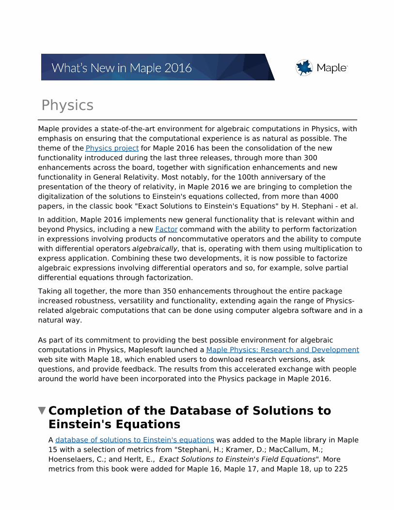
PhysicsMaple provides a state-of-the-art environment for algebraic computations in Physics, with emphasis on ensuring that the computational experience is as natural as possible. The theme of the Physics project for Maple 2016 has been the consolidation of the new functionality introduced during the last three releases, through more than 300 enhancements across the board, together with signification enhancements and new functionality in General Relativity. Most notably, for the 100th anniversary of the presentation of the theory of relativity, in Maple 2016 we are bringing to completion the digitalization of the solutions to Einstein's equations collected, from more than 4000 papers, in the classic book "Exact Solutions to Einstein's Equations" by H. Stephani - et al.
In addition, Maple 2016 implements new general functionality that is relevant within and beyond Physics, including a new Factor command with the ability to perform factorization in expressions involving products of noncommutative operators and the ability to compute with differential operators algebraically, that is, operating with them using multiplication toexpress application. Combining these two developments, it is now possible to factorize algebraic expressions involving differential operators and so, for example, solve partial differential equations through factorization.
Taking all together, the more than 350 enhancements throughout the entire package increased robustness, versatility and functionality, extending again the range of Physics-related algebraic computations that can be done using computer algebra software and in anatural way.
As part of its commitment to providing the best possible environment for algebraic computations in Physics, Maplesoft launched a Maple Physics: Research and Development web site with Maple 18, which enabled users to download research versions, ask questions, and provide feedback. The results from this accelerated exchange with people around the world have been incorporated into the Physics package in Maple 2016.
Completion of the Database of Solutions to Einstein's EquationsA database of solutions to Einstein's equations was added to the Maple library in Maple 15 with a selection of metrics from "Stephani, H.; Kramer, D.; MacCallum, M.; Hoenselaers, C.; and Herlt, E., Exact Solutions to Einstein's Field Equations". More metrics from this book were added for Maple 16, Maple 17, and Maple 18, up to 225

> >
(1)(1)
> >
metrics. In Maple 2016, for the 100th anniversary of the presentation of the theory of Relativity by A. Einstein, we brought to completion the digitalization of all the 971 metric solutions collected from more than 4000 papers presented in the General Relativity literature. All these metrics can be loaded or searched using g_ (the Physics command representing the spacetime metric that also sets the metric to your choice in one go) or using the command DifferentialGeometry:-Library:-MetricSearch. When a metric is loaded, all the General Relativity tensors (Christoffel, Ricci, Einstein, and Riemann) are automatically computed on background and available for further computations. These metrics can also be changed in various ways and, automatically, all the General Relativity tensors are recomputed on background. You can work with these metrics, the ones in the database or any other one you set, using the Tetrads formalism too, with the commands of the Physics:-Tetrads package.
In the Maple PDEtools package, you have the mathematical tools - including a complete symmetry approach - to work with the underlying partial differential equations. By combining the functionality of the Physics:-Tetrads package, the Physics:-TransformCoordinates command, and the ability to compute Riemann and Weyl invariants, you can also formulate and, depending on the the metrics also resolve, the equivalence problem; that is: to answer whether or not, given two metrics, they can be obtained from each other by a transformation of coordinates, as well as compute the transformation.
Examples
Load Physics, set the metric to Schwarzschild (and everything else automatically) in one go
That is all you need to do: although the strength in Physics is to compute with tensors using indicial notation, by setting the metric as in (1) all of the tensor components of the General Relativity tensors are also derived on the fly and ready

> >
> >
> >
> >
(5)(5)
> >
(6)(6)
(7)(7)
(2)(2)
(3)(3)
(4)(4)
> >
for use. For instance these are the definition in terms of Christoffel symbols, and the covariant components of the Ricci tensor for Schwarzschild solution
These are the 16 Riemann invariants for Schwarzschild solution, using the formulas by Carminati and McLenaghan
The related Weyl scalars in the context of the Newman-Penrose formalism; the definition is in terms of the Weyl tensor and the tetrad of tensors of the
Newman-Penrose formalism
These are the matrix components of the Christoffel symbols of the second kind (that describe, in coordinates, the effects of parallel transport in curved surfaces), when the first of its three indices is equal to 1; contravariant indices are prefixed by ~

(8)(8)
(9)(9)
(7)(7)
> >
> >
In Physics, the Christoffel symbols of the first kind are represented by the same object (one command, Christoffel, not two) just by taking the first index covariant, aswe do when computing with paper and pencil
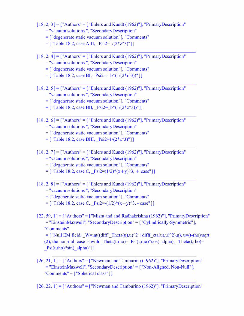
One could query the database, directly from the spacetime metrics, for example about the solutions (metrics) to Einstein's equations related to Levi-Civita, the Italian mathematician
____________________________________________________________
____________________________________________________________
____________________________________________________________
____________________________________________________________
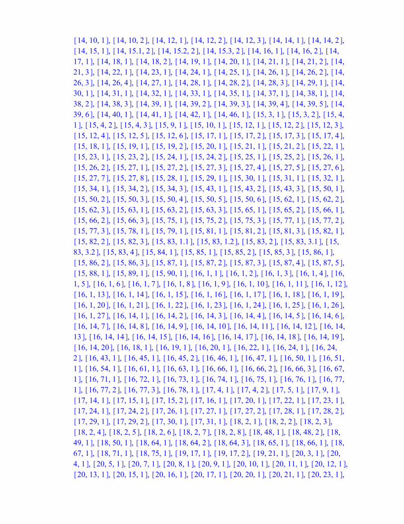
Each triad of numbers indicates the chapter and equation number with which each of

> >
> >
(12)(12)
> >
(7)(7)
(10)(10)
(11)(11)
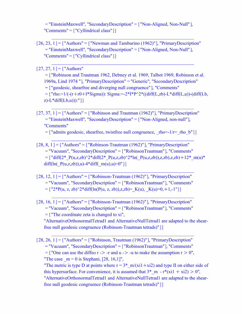
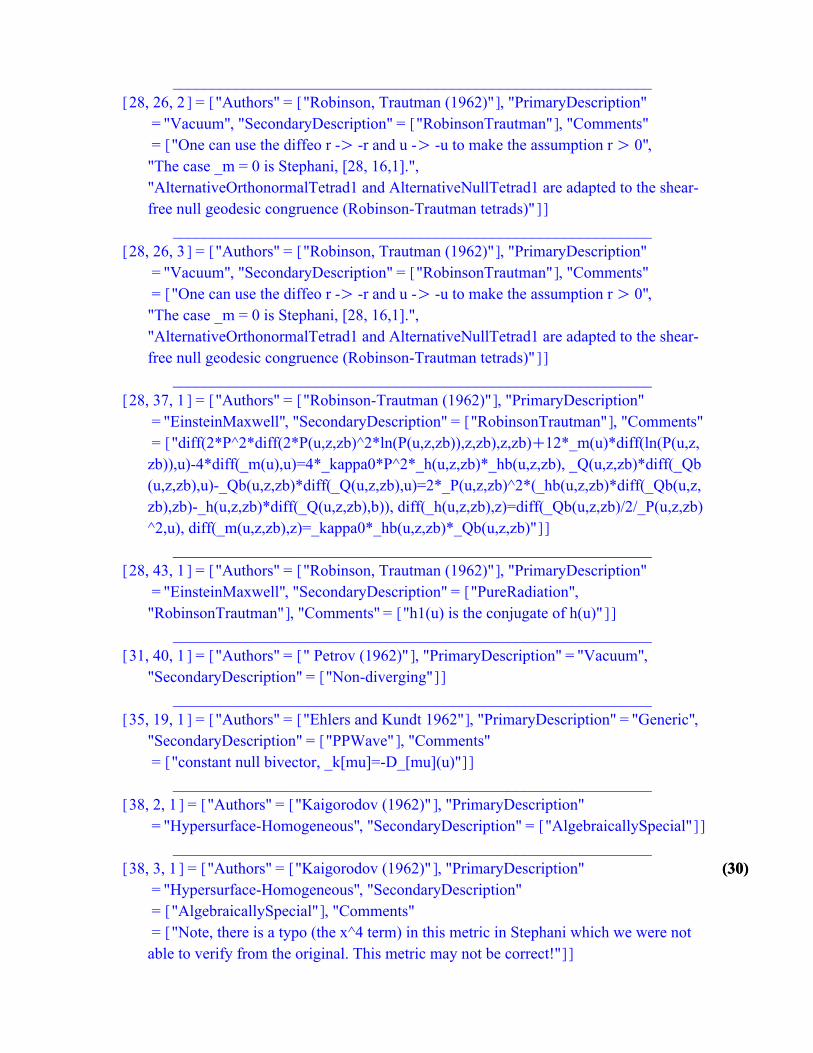
these metrics appear in "Exact Solutions to Einstein's Field Equations". For example, [12, 16, 1] is the metric found in Chapter 12 with equation number 16.1. These solutions can be set in one go from the metrics command, just by indicating the triadof numbers as follows
Resetting the signature of spacetime from "C - - -" to `- C C C` in order to match the signature in the database of metrics:
Automatically, everything gets set accordingly; these are the contravariant components of the related Ricci tensor
One works with the Newman-Penrose formalism frequently using tetrads (local system of references); the Physics subpackage for this is Tetrads
Setting lowercaselatin letters to represent tetrad indices
(13)(13)
(16)(16)
> >
> >
(12)(12)
(15)(15)
(14)(14)
> >
> >
> >
(7)(7)
> >
(17)(17)
(18)(18)
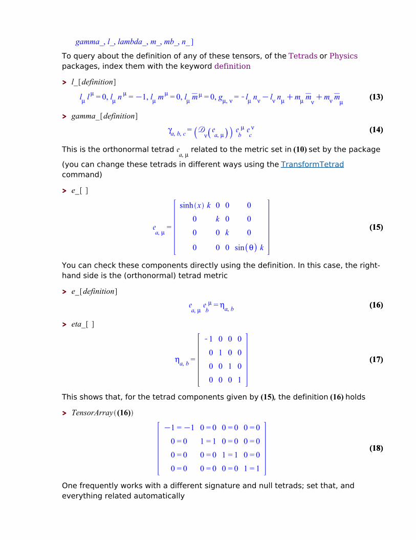
To query about the definition of any of these tensors, of the Tetrads or Physics packages, index them with the keyword definition
This is the orthonormal tetrad related to the metric set in (10) set by the package
(you can change these tetrads in different ways using the TransformTetrad command)
You can check these components directly using the definition. In this case, the right-hand side is the (orthonormal) tetrad metric
This shows that, for the tetrad components given by (15), the definition (16) holds
One frequently works with a different signature and null tetrads; set that, and everything related automatically

(19)(19)> >
> >
(12)(12)
> >
> >
> >
(7)(7)
(23)(23)> >
(22)(22)
(21)(21)
> >
(20)(20)
(24)(24)
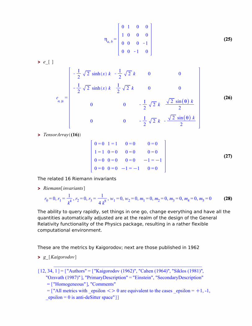
(25)(25)
Verifying (21) using the definition (16)
You can also change the signature and everything gets automatically recomputed aswell, from the components of the tensors to the definition of Weyl scalars. You can query the value of the signature using Setup
Set the signature to be + - - - , compare the components of the null tetrad metric with the components of (20) and verify the tetrad
(29)(29)
> >
(19)(19)> >
> >
(12)(12)
> >
(27)(27)
(26)(26)
(7)(7)
(28)(28)
> >
(25)(25)
The related 16 Riemann invariants
The ability to query rapidly, set things in one go, change everything and have all the quantities automatically adjusted are at the realm of the design of the General Relativity functionality of the Physics package, resulting in a rather flexible computational environment.
These are the metrics by Kaigorodov; next are those published in 1962
____________________________________________________________

> >
(12)(12)
(7)(7)
(25)(25)
(29)(29)
(19)(19)
(30)(30)
> >
____________________________________________________________
____________________________________________________________
____________________________________________________________
____________________________________________________________
____________________________________________________________
____________________________________________________________
____________________________________________________________
____________________________________________________________
____________________________________________________________
____________________________________________________________
> >
(12)(12)
(7)(7)
(25)(25)
(29)(29)
(19)(19)
(30)(30)
____________________________________________________________
____________________________________________________________
____________________________________________________________
____________________________________________________________
____________________________________________________________
____________________________________________________________
____________________________________________________________
____________________________________________________________
> >
(12)(12)
(7)(7)
(25)(25)
(29)(29)
(19)(19)
(30)(30)
____________________________________________________________
____________________________________________________________
____________________________________________________________
____________________________________________________________
____________________________________________________________
____________________________________________________________
____________________________________________________________
____________________________________________________________

(29)(29)
(19)(19)> >
(30)(30)
(12)(12)
(31)(31)
(7)(7)
> >
> >
(25)(25)
The search can also be done visually, by properties. The following is the only solutionin the database that is a Pure Radiation solution, of Petrov Type "D", Plebanski-PetrovType "O" and that has Isometry Dimension equal to 1:
Set the solution, and everything related to work with it, in one go
Resetting the signature of spacetime from "C - - -" to `- C C C` in order to match the signature in the database of metrics:

(29)(29)
> >
(19)(19)> >
(30)(30)
(12)(12)
(31)(31)
(7)(7)
(32)(32)
> >
(33)(33)
(25)(25)
The related Riemann invariants:
To list all the triads of numbers associated to the solutions digitized in the database (each triad indicates the Chapter and equation number with which each of these metrics appear in the book), enter
(29)(29)
(19)(19)> >
(30)(30)
(12)(12)
(31)(31)
(7)(7)
(33)(33)
(25)(25)

(29)(29)
(19)(19)> >
(30)(30)
(12)(12)
(31)(31)
(7)(7)
(33)(33)
(25)(25)

> >
(12)(12)
(34)(34)
(31)(31)
(7)(7)
(33)(33)
(25)(25)
(29)(29)
(19)(19)
(30)(30)
> >
There are as many solutions as
971
Operatorial Algebraic Expressions Involving the

> >
> >
(37)(37)
(12)(12)
(31)(31)
(7)(7)
(33)(33)
> >
(25)(25)
> >
(29)(29)
(19)(19)
(30)(30)
(35)(35)
> >
(36)(36)
Differential Operators , and (nabla)
Maple 2016 implements the concept of operatorial expressions, that is, the ability to compute with the differential operators , and nabla from the Vectors
subpackage, algebraically, considering them as noncommutative operators and using multiplication to express their application within expressions. When desired, themultiplication is transformed into application of the differential operator to the operandsthat appear to its right.
The differential operators , and nabla are thus now considered
noncommutative, in that and they are assumed to commute only with mathematical objects that do not depend on the coordinates (that is, constants with respect to their differentiation variables). This also means that the Commutator and Anticommutator commands, as well as the commands Library:-Commute and Library:-Anticommute, all work with these differential operators taking their noncommutative property into account.
Among other things, this new ability to compute with differential operators algebraically, when combined with the new ability to factorize expressions involving products of noncommutative operands, allows for factorizing algebraic expressions representing differential operators of higher order into products of algebraic expressions representing differential operators of lower order - an operation at the realm of solving non-linear differential equations; the first steps of this approach are now implemented too.
Examples
Consider the commutator between a scalar and the nabla operator ; use compact display for convenience
New: the expanded form of this commutator now has the correct operatorial meaning:

(41)(41)
> >
> >
> >
(12)(12)
> >
> >
(31)(31)
(7)(7)
(45)(45)
> >
(33)(33)
(25)(25)
> >
(44)(44)
(29)(29)
> >
(38)(38)
(19)(19)
(30)(30)
(39)(39)
> >
(40)(40)
> >
(43)(43)
(42)(42)
(46)(46)
So all the algebra is performed taking as a noncommutative operator, as we do when computing with paper and pencil. You can apply the differential operators at any time using the new Library:-ApplyProductsOfDifferentialOperators
The underlying types working at the core of this implementation of operatorial expressions
true
true
false
The differentiation variables associated to are the coordinates of the Cartesian cylindrical and spherical systems of coordinates: .
The same concept is implemented for the differential operators of special and general relativity, , and . Define system of coordinates, X, then A and B as a
tensors and for convenience use a compact display
Defined objects with tensor properties
The commutator of and multiplied by B , representing the application of can
now be represented as

(52)(52)
(50)(50)
> >
> >
(54)(54)
(12)(12)
> >
> >
> >
(31)(31)
(7)(7)
> >
> >
(33)(33)
> >
(25)(25)
(55)(55)
(29)(29)
(38)(38)
(19)(19)
(30)(30)
(47)(47)
> >
> >
(49)(49)
(51)(51)
(53)(53)
(48)(48)
> >
Note that to the right of in the first term there is the product , so that when
applying the operator to the product, two terms result, one of which cancels the second term in (48)
As an example of the possibilities open with operatorial algebraic expressions combined with the new factorization of algebraic expressions involving noncommutative objects, consider the factorization of Laplace equation in a Euclidean space
* Partial match of 'coordinates' against keyword 'coordinatesystems'
The Euclidean metric in cartesian coordinatesChanging the signature of the tensor spacetime to: C C C C
Similar problem now with vectorial differential operators, split into time and space components,

> >
(61)(61)
> >
(62)(62)
(12)(12)
> >
(31)(31)
(7)(7)
> >
> >
> >
(60)(60)
(33)(33)
(25)(25)
(29)(29)
(58)(58)
(38)(38)
(19)(19)
(30)(30)
(59)(59)
(47)(47)
(57)(57)
(56)(56)
> >
> >
> >
(63)(63)
> >
> >
The same functionality is implemented for , the covariant derivative operator. Set
the spacetime to be curved, for instance using Schwarzschild's metric and redefine the compact display to use the new (spherical) coordinates
The commutator of covariant derivatives
Multiply this result by a tensor function of the coordinates, say defined in the
lines above
Apply the differential operators

> >
> >
> >
> >
(64)(64)
(66)(66)
> >
(12)(12)
(65)(65)
(31)(31)
(7)(7)
(68)(68)
> >
> >
> >
(33)(33)
(70)(70)
(25)(25)
(29)(29)
(71)(71)
(67)(67)
(38)(38)
(19)(19)
(30)(30)
(69)(69)
(47)(47)
(56)(56)
> >
> >
(63)(63)
> >
> >
Compare with the expanded version before applying, i.e.: the same expression but expressed algebraically using multiplication instead of application
The Bianchi identity can be expressed in terms of commutators
Expand the first commutator
Expand the whole identity
Let D_[mu] be the covariant derivative of gauge theory with A[mu] representing the gauge field; for the current signature,
we have
I
Note that the gauge field is introduced depending on the coordinates, which are omitted from the display due to the use of PDEtools:-declare in (59). Introduce now this definition in the Bianchi identity
Expand the first commutator

> >
> >
(12)(12)
> >
> >
(79)(79)
(77)(77)
(31)(31)
> >
(7)(7)
(75)(75)
(73)(73)
(78)(78)
> >
(72)(72)
(33)(33)
(25)(25)
(29)(29)
(38)(38)
(19)(19)
> >
(30)(30)
(47)(47)
> >
> >
(56)(56)
> >
> >
> >
(80)(80)
(76)(76)
(74)(74)
(63)(63)
> >
Expand the whole identity
Apply the operatorial expression (72) to a function of the coordinates
Apply the inner commutator of the first term of (71)
Factorization of Expressions Involving Noncommutative OperatorsOne of the interesting things about the Physics package is that it was designed from scratch to extend the domain of operations of the Maple system from commutative variables to one that includes commutative, anticommutative and noncommutative variables, as well as abstract vectors and related (nabla) differential operators. In this line we have, among others, the following Physics commands working with this extended domain:
> >
> >
(81)(81)
(12)(12)
> >
(31)(31)
(7)(7)
(83)(83)
> >
> >
(72)(72)
(33)(33)
> >
(25)(25)
(29)(29)
(38)(38)
(19)(19)
(30)(30)
(47)(47)
(82)(82)
(56)(56)
(84)(84)
> >
> >
(63)(63)
> >
(85)(85)
> >
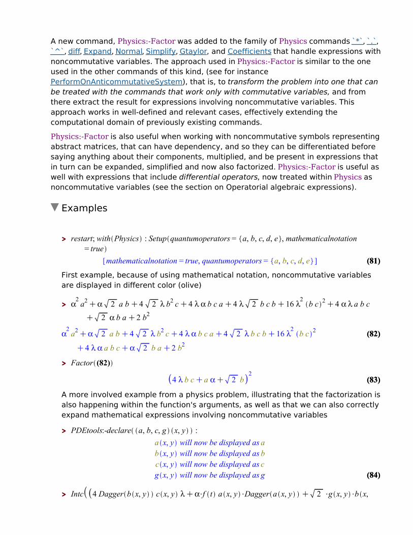
A new command, Physics:-Factor was added to the family of Physics commands ̀ *`, ̀ .`,`^`, diff, Expand, Normal, Simplify, Gtaylor, and Coefficients that handle expressions withnoncommutative variables. The approach used in Physics:-Factor is similar to the one used in the other commands of this kind, (see for instancePerformOnAnticommutativeSystem), that is, to transform the problem into one that can be treated with the commands that work only with commutative variables, and from there extract the result for expressions involving noncommutative variables. This approach works in well-defined and relevant cases, effectively extending the computational domain of previously existing commands.
Physics:-Factor is also useful when working with noncommutative symbols representingabstract matrices, that can have dependency, and so they can be differentiated before saying anything about their components, multiplied, and be present in expressions that in turn can be expanded, simplified and now also factorized. Physics:-Factor is useful aswell with expressions that include differential operators, now treated within Physics as noncommutative variables (see the section on Operatorial algebraic expressions).
Examples
First example, because of using mathematical notation, noncommutative variables are displayed in different color (olive)
2
A more involved example from a physics problem, illustrating that the factorization isalso happening within the function's arguments, as well as that we can also correctlyexpand mathematical expressions involving noncommutative variables

(86)(86)
> >
(88)(88)
(12)(12)
> >
(90)(90)
(31)(31)
> >
(7)(7)
> >
(87)(87)
> >
(72)(72)
(89)(89)
(33)(33)
(25)(25)
(29)(29)
> >
(38)(38)
> >
(19)(19)
> >
(30)(30)
(47)(47)
(56)(56)
> >
> >
> >
(63)(63)
> >
(91)(91)
(85)(85)
(92)(92)
> >
So first expand
Now retrieve the original expression by recursing over the arguments in order to factor the integrand
This following one looks simpler but it is actually more complicated:
The complication consists of the fact that the standard factor command, that assumes products are commutative, can never deal with an expression like
because if products were commutative the sum of these terms is equal to 0. Through algebraic manipulations, however, the expression is also factorable
This other one is yet more complicated:
When you expand,
there are various terms involving the same noncommutative operands, just multiplied in a different order. Generally speaking the limitation of this approach (in
> >
> >
(12)(12)
> >
(95)(95)
(31)(31)
(7)(7)
> >
> >
> >
> >
(72)(72)
(33)(33)
(25)(25)
(93)(93)
> >
(29)(29)
(96)(96)
(38)(38)
(19)(19)
(97)(97)
(30)(30)
(47)(47)
(56)(56)
> >
> >
(63)(63)
(94)(94)
(85)(85)
> >
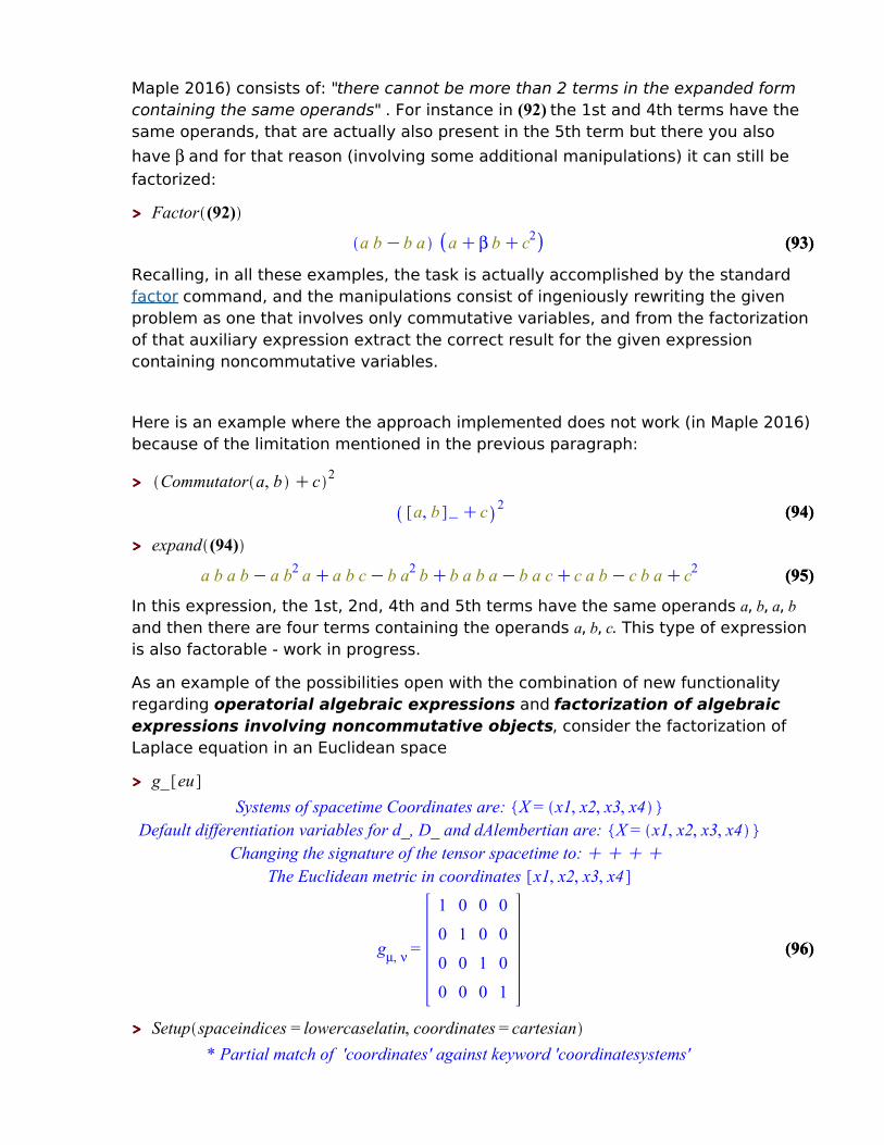
Maple 2016) consists of: "there cannot be more than 2 terms in the expanded form containing the same operands" . For instance in (92) the 1st and 4th terms have the same operands, that are actually also present in the 5th term but there you also have and for that reason (involving some additional manipulations) it can still be factorized:
Recalling, in all these examples, the task is actually accomplished by the standardfactor command, and the manipulations consist of ingeniously rewriting the given problem as one that involves only commutative variables, and from the factorization of that auxiliary expression extract the correct result for the given expression containing noncommutative variables.
Here is an example where the approach implemented does not work (in Maple 2016) because of the limitation mentioned in the previous paragraph:
2
In this expression, the 1st, 2nd, 4th and 5th terms have the same operands , , , and then there are four terms containing the operands , , . This type of expression is also factorable - work in progress.
As an example of the possibilities open with the combination of new functionality regarding operatorial algebraic expressions and factorization of algebraic expressions involving noncommutative objects, consider the factorization of Laplace equation in an Euclidean space
Changing the signature of the tensor spacetime to: C C C C
* Partial match of 'coordinates' against keyword 'coordinatesystems'
> >
> >
> >
> >
(12)(12)
(100)(100)
> >
(101)(101)
(31)(31)
(7)(7)
> >
(102)(102)
> >
> >
(72)(72)
> >
(33)(33)
(98)(98)
(25)(25)
(104)(104)
(103)(103)
(29)(29)
(38)(38)
> >
(19)(19)
(97)(97)
(30)(30)
(47)(47)
(56)(56)
> >
> >
(63)(63)
(99)(99)
(85)(85)
> >
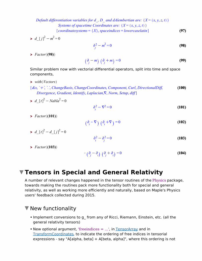
Similar problem now with vectorial differential operators, split into time and space components,
Tensors in Special and General RelativityA number of relevant changes happened in the tensor routines of the Physics package, towards making the routines pack more functionality both for special and general relativity, as well as working more efficiently and naturally, based on Maple's Physics users' feedback collected during 2015.
New functionalityImplement conversions to g_ from any of Ricci, Riemann, Einstein, etc. (all the general relativity tensors)
New optional argument, 'freeindices = ...', in TensorArray and inTransformCoordinates, to indicate the ordering of free indices in tensorial expressions - say "A[alpha, beta] + A[beta, alpha]", where this ordering is not

> >
> >
(108)(108)
(12)(12)
(106)(106)
> >
> >
(31)(31)
(107)(107)
(7)(7)
> >
> >
(72)(72)
(33)(33)
(25)(25)
(29)(29)
(38)(38)
(19)(19)
(97)(97)
(30)(30)
(105)(105)
(47)(47)
(56)(56)
> >
> >
> >
(63)(63)
(85)(85)
> >
obvious, including now a new subroutine to determine this ordering in a predictable way and regardless of whether the indices are covariant or contravariant.
Implement option 'specializeconstants' within Physics:-KillingVectors
Examples
Rewrite the general relativity tensors in terms of the metric (convert to g_)Set the spacetime to something not flat, for instance Schwarzschild's solution
R
This is the standard definition of the Ricci tensor in terms of Christoffel symbols
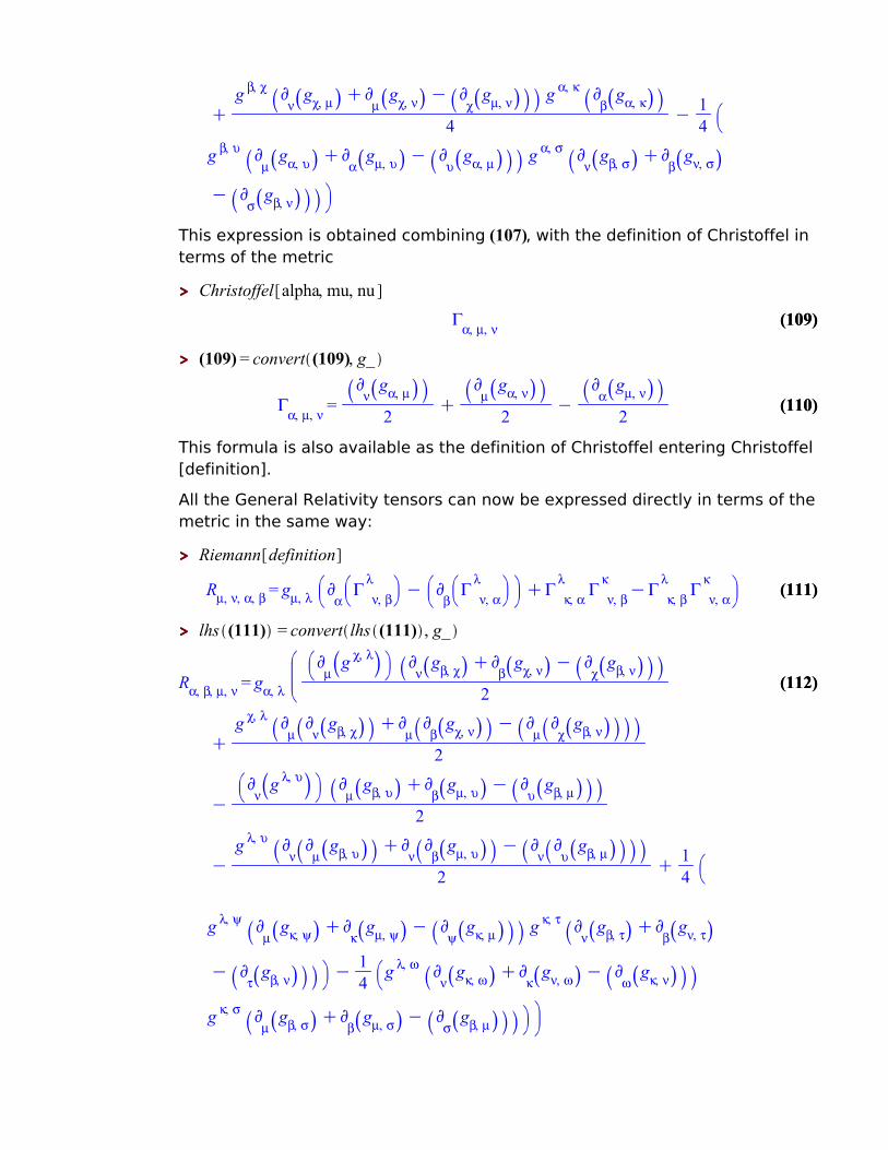
When computing field equations, however, we need the expression of the Ricci tensor directly in terms of the metric
> >
(108)(108)
(12)(12)
> >
> >
(31)(31)
(111)(111)
(7)(7)
(109)(109)
> >
> >
(72)(72)
(33)(33)
(110)(110)
(25)(25)
(29)(29)
(38)(38)
(19)(19)
(97)(97)
(30)(30)
(112)(112)
(47)(47)
(56)(56)
> >
> >
> >
(63)(63)
> >
(85)(85)
> >
This expression is obtained combining (107), with the definition of Christoffel in terms of the metric
This formula is also available as the definition of Christoffel entering Christoffel[definition].
All the General Relativity tensors can now be expressed directly in terms of themetric in the same way:
> >
> >
> >
(108)(108)
(12)(12)
> >
(31)(31)
(7)(7)
(116)(116)
> >
(115)(115)
> >
(72)(72)
(33)(33)
(25)(25)
> >
(29)(29)
(38)(38)
(19)(19)
(97)(97)
(30)(30)
> >
(114)(114)
(47)(47)
(56)(56)
(113)(113)
> >
> >
(63)(63)
(85)(85)
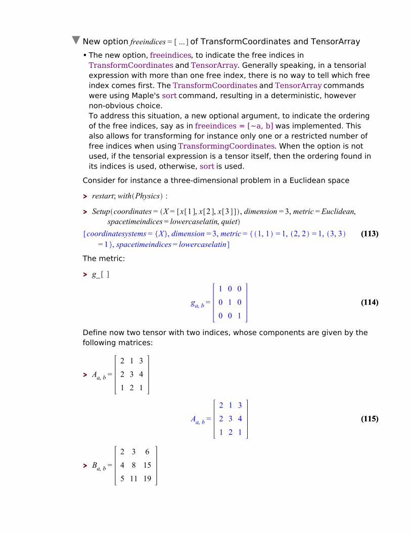
> >
New option of TransformCoordinates and TensorArrayThe new option, freeindices, to indicate the free indices inTransformCoordinates and TensorArray. Generally speaking, in a tensorial expression with more than one free index, there is no way to tell which free index comes first. The TransformCoordinates and TensorArray commands were using Maple's sort command, resulting in a deterministic, however non-obvious choice.To address this situation, a new optional argument, to indicate the ordering of the free indices, say as in freeindices = [~a, b] was implemented. This also allows for transforming for instance only one or a restricted number of free indices when using TransformingCoordinates. When the option is not used, if the tensorial expression is a tensor itself, then the ordering found inits indices is used, otherwise, sort is used.
Consider for instance a three-dimensional problem in a Euclidean space
The metric:
Define now two tensor with two indices, whose components are given by the following matrices:
> >
(108)(108)
(122)(122)
> >
(12)(12)
> >
(31)(31)
(7)(7)
(121)(121)
> >
(116)(116)
> >
> >
(72)(72)
(33)(33)
(118)(118)
(25)(25)
> >
(29)(29)
(38)(38)
(19)(19)
> >
(97)(97)
(30)(30)
(47)(47)
(56)(56)
(119)(119)
> >
> >
(120)(120)
(63)(63)
(85)(85)
(117)(117)
> >
> >
Defined objects with tensor properties
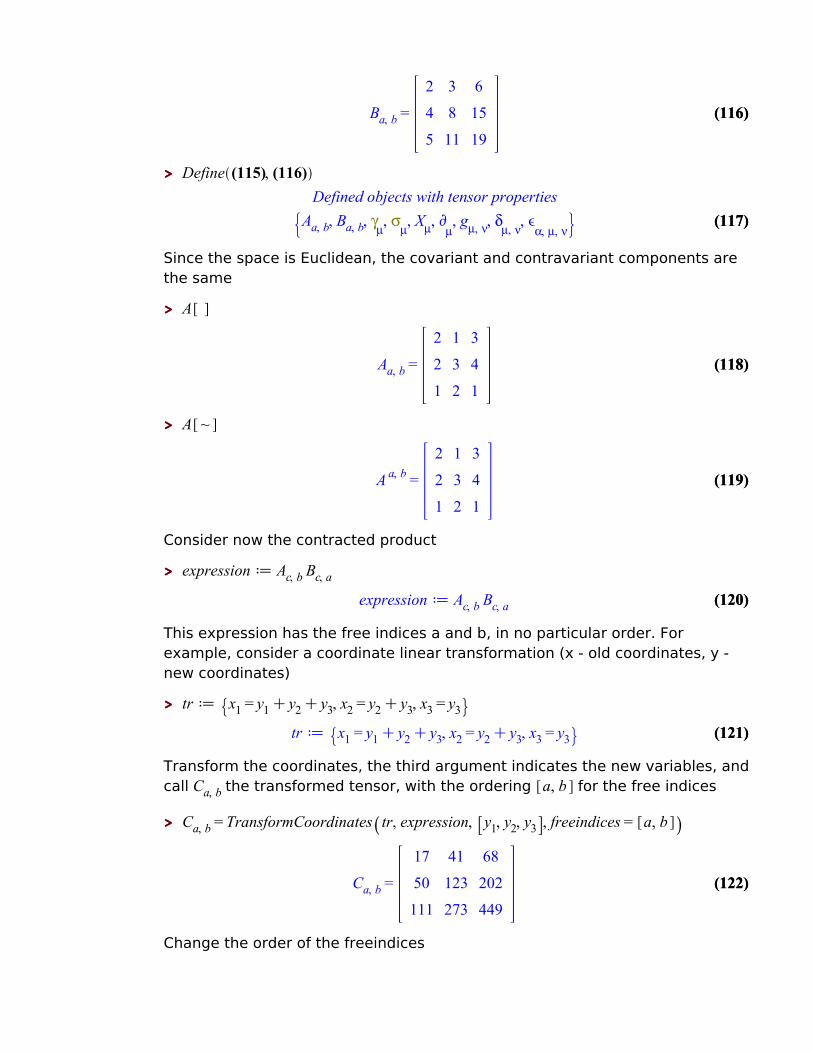
Since the space is Euclidean, the covariant and contravariant components are the same
Consider now the contracted product
This expression has the free indices a and b, in no particular order. For example, consider a coordinate linear transformation (x - old coordinates, y - new coordinates)
Transform the coordinates, the third argument indicates the new variables, andcall the transformed tensor, with the ordering for the free indices
Change the order of the freeindices

> >
(108)(108)
(12)(12)
> >
> >
(125)(125)
(31)(31)
(7)(7)
(126)(126)
(127)(127)
(116)(116)
> >
> >
> >
(72)(72)
(33)(33)
(25)(25)
(29)(29)
(123)(123)
(38)(38)
(19)(19)
(97)(97)
(30)(30)
(47)(47)
> >
(56)(56)
(124)(124)
> >
> >
(63)(63)
(85)(85)
> >
> >
Transform only one index, first , then , then in sequence
The same option is now available for TensorArray. Compute the tensor components of the tensorial expression (120) using the two possible orderings of its free indices
New option of KillingVectorsThe design of KillingVectors was revised for Maple 2016 with regards to: a) return the Killing vectors using a vector format, not just the solution to the underlying PDE system, b) compute their contravariant components by default instead of covariant; c) introduce a new keyword specializeconstants to

(129)(129)
> >
> >
(128)(128)
(108)(108)
(12)(12)
(116)(116)
> >
(132)(132)
(33)(33)
> >
(25)(25)
(19)(19)
(131)(131)
(97)(97)
> >
> >
(63)(63)
(85)(85)
> >
> >
> >
(31)(31)
(7)(7)
(130)(130)
> >
> >
> >
(72)(72)
(29)(29)
(123)(123)
(38)(38)
(30)(30)
(47)(47)
(56)(56)
> >
request the specialization of the constants that appear when solving the underlying linear PDE system.
Set a system of Coordinates
* Partial match of 'coordinates' against keyword 'coordinatesystems'
Define a tensor with one index to represent the Killing vector
Defined objects with tensor properties
The components of the contravariant , directly in list format, ready to be forwarded to Define to compute furthermore with them:
The same result but this time for the covariant components (for that purpose, pass with a covariant index), and without specializing the integration constants,
* Partial match of 'specialize' against keyword 'specializeconstants'
The new format for the output of KillingVectors facilitates computing with these results. For example, define V as a tensor using the first Killing vector solution in (131), check its contravariant and covariant components, and verify that it is indeed a Killing Vector by verifying the definition in terms of Lie derivatives.
Define (131)[1] as a tensor

> >
> >
(108)(108)
(139)(139)
(12)(12)
(135)(135)
(116)(116)
(33)(33)
(25)(25)
(19)(19)
(97)(97)
(137)(137)
(133)(133)
> >
> >
(138)(138)
> >
(63)(63)
(85)(85)
> >
> >
> >
> >
> >
(31)(31)
(7)(7)
> >
> >
(72)(72)
(134)(134)
(29)(29)
(136)(136)
(123)(123)
(38)(38)
(30)(30)
(47)(47)
(56)(56)
> >
Defined objects with tensor properties
Check the covariant and contravariant components of
Verify that is indeed a Killing Vector, that is, that the Lie derivative of the metric with respect to the is 0
V
Compute the components of this tensorial equation
Improved functionalityInstall new approach for computing the Weyl scalars ~10x faster; fix issue noticed during development (missing clearing a cache) and add test with difficult example (Kerr metric) for the computation of Weyl scalars
4x speedup in the computation of the Ricci scalars (testing example: the Kerr metric)
5x speedup in the computation of the components of the Ricci tensor in the case of an arbitrary spacetime metric (10 unknown functions of 4 independent variables each).
Examples

> >
> >
> >
(108)(108)
(12)(12)
(116)(116)
(33)(33)
(25)(25)
(19)(19)
(97)(97)
(133)(133)
> >
> >
(140)(140)
(63)(63)
(141)(141)
(85)(85)
> >
> >
> >
(31)(31)
(7)(7)
> >
> >
(72)(72)
(29)(29)
(123)(123)
(38)(38)
(30)(30)
(47)(47)
(56)(56)
> >
> >
Depending on the form of the spacetime metric, the computation of the Weyl and Ricci scalars, or the components of the Ricci tensor, can be rather involved, requiring handling large algebraic expressions depending on mathematical functions. Improving the approach for these kinds of difficult algebraic computations is one area of constant development.
Consider the Kerr solution in terms of Boyer and Lindquist coordinates, shown in Chapter 5 (equation 5.29) of the book "The large scale structure of space-time" byS. W. Hawking and G. F. R. Ellis; the corresponding line element
Set the coordinates, and the metric using this line element all in one go
* Partial match of 'coordinates' against keyword 'coordinatesystems'Detected `t`, the time variable, in position 1. Changing the signature of the spacetime
metric accordingly, to: C - - -
Check the metric

> >
> >
(108)(108)
(12)(12)
> >
(31)(31)
(7)(7)
(116)(116)
> >
> >
(72)(72)
(33)(33)
(25)(25)
(142)(142)
(143)(143)
(29)(29)
(123)(123)
(38)(38)
(19)(19)
(97)(97)
(30)(30)
(47)(47)
(133)(133)
(56)(56)
> >
> >
> >
(63)(63)
(141)(141)
> >
(85)(85)
> >
The Weyl scalars for this metric are now computed 10x faster than in Maple 2015.Their definition in terms of the four vectors l , n , m , m of the Newman-Penrose
formalism
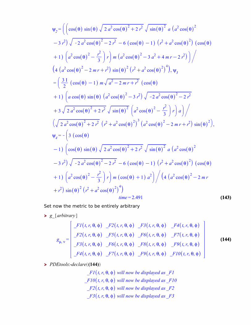
The five Weyl scalars defined above and the time to compute them
> >
(108)(108)
(145)(145)
(12)(12)
> >
(31)(31)
(7)(7)
(116)(116)
> >
> >
(72)(72)
(33)(33)
(25)(25)
(143)(143)
(29)(29)
(123)(123)
(38)(38)
(19)(19)
> >
(97)(97)
(30)(30)
(47)(47)
> >
(133)(133)
(56)(56)
(144)(144)
> >
> >
> >
(63)(63)
(141)(141)
(85)(85)
> >
Set now the metric to be entirely arbitrary

> >
(108)(108)
(145)(145)
(12)(12)
(116)(116)
(148)(148)
> >
(33)(33)
(25)(25)
(19)(19)
(97)(97)
> >
(133)(133)
(149)(149)
> >
(147)(147)
> >
(63)(63)
(141)(141)
(85)(85)
> >
> >
(31)(31)
> >
(7)(7)
> >
> >
> >
(72)(72)
(146)(146)
(143)(143)
(29)(29)
(123)(123)
(38)(38)
(30)(30)
(47)(47)
(56)(56)
> >
> >
In Maple 2015, on a typical fast machine, the computation of the Ricci tensor components was taking around 1 minute. After an optimization of the code it now takes around 12 seconds (avoid displaying the components themselves to not clutter the display with too large expressions)
The computational length of all the algebraic expressions entering these components is
36613509
Vectors PackageA number of enhancements were performed in the Vectors subpackage:
You can now represent the scalar product of a vector with itself by a squaring (power2) of the vector.
You can now add vectors of different bases and change basis in expressions that contain unit vectors of different orthonormal basis.
Examples
Consider the relativistic Hamiltonian of a particle of mass m; you can now enter the square of the momentum (scalar product of p with itself) directly as a power, as we do when computing with paper and pencil
The expansion of the power of a vector now returns the square of its norm

(155)(155)
(150)(150)
> >
(108)(108)
(145)(145)
> >
(12)(12)
> >
> >
(116)(116)
(33)(33)
(25)(25)
(19)(19)
(97)(97)
> >
> >
(133)(133)
(149)(149)
(157)(157)
> >
> >
> >
(63)(63)
(141)(141)
(85)(85)
> >
> >
(31)(31)
(7)(7)
(153)(153)
> >
> >
(72)(72)
(154)(154)
(143)(143)
(29)(29)
(123)(123)
(38)(38)
(152)(152)
(30)(30)
(151)(151)
(47)(47)
(56)(56)
(156)(156)
> >
> >
> >
Introduce now the components of p
Now H, or its expanded form, are given by
Likewise, the expansion computed before entering the components of p now appearsas
Consider the following vectorial expression where the right-hand-side involves unit vectors and coordinates of both the cylindrical and spherical basis
Change all to the spherical basis, also the coordinates
* Partial match of 'also' against keyword 'alsocomponents'
The same operation to the cylindrical basis

(158)(158)
> >
> >
(108)(108)
(145)(145)
(12)(12)
(116)(116)
(33)(33)
(25)(25)
(19)(19)
(97)(97)
(133)(133)
(149)(149)
> >
> >
(63)(63)
(141)(141)
(85)(85)
> >
> >
(31)(31)
(7)(7)
> >
> >
(72)(72)
(143)(143)
(29)(29)
(123)(123)
(38)(38)
(30)(30)
(47)(47)
(56)(56)
> >
* Partial match of 'also' against keyword 'alsocomponents'
The Physics LibraryFour new commands, useful for programming and interactive computation, have been added to the Physics:-Library package, that now includes 142 documented commands. These new ones are:
ApplyProductsOfDifferentialOperators
DelayEvaluationOfTensors
PerformMatrixOperations
ShowTypeDefinition
Additionally, eight new types, related to the developments in Physics for Maple 2016, were added to the Physics:-Library:-PhysicsType subpackage of Physics types, for programming or interactive purposes. These are
DifferentialOperator, DifferentialOperatorIndexed, DifferentialOperatorSymbol, EuclideanIndex, ExtendedDifferentialOperator, ExtendedDifferentialOperatorIndexed, ExtendedDifferentialOperatorSymbol, TensorWithNumericalIndices
Redesigned Functionality and MiscellaneousRedesign of D_[mu] to not prematurely evaluate the argument.
Reimplementing Physics:-Dgamma as a tensor with Array representation instead of an (old) matrix.
d_[mu](x1) used to return g_[mu,~1], which generally speaking is correct, but in a curved spacetime this result is incorrect because d_[mu](x1) is not a tensor while g_[mu,1] is used as a tensor. For example, taking the covariant derivative of d_[mu](X[`~1`]) = g_[mu, `~1`] one would get zero on the right-hand side but not zero on the left-hand side. This is corrected so that d_[mu](x1) does not return g_[mu,~1] anymore when the spacetime is curved.
Change default in KillingVectors: when the vector V is passed without indices, the equations for the contravariant V (not the covariant) are solved.
Change in default of Physics:-KillingVectors: now it returns with all the integration constants specialized, unless a (new) optional keyword 'specializeconstants = false' is passed.
(158)(158)
> >
> >
(108)(108)
(145)(145)
(12)(12)
> >
(31)(31)
(7)(7)
(116)(116)
> >
> >
(72)(72)
(33)(33)
(25)(25)
(143)(143)
(29)(29)
(123)(123)
(38)(38)
(19)(19)
(97)(97)
(30)(30)
(47)(47)
(133)(133)
(56)(56)
> >
(149)(149)
> >
> >
(63)(63)
(141)(141)
(85)(85)
> >
Adjust design in Physics:-LieBrackets: when the related LieDerivative returns 0,LieBracket now returns an n-dimensional Array where n is the spacetime dimension and all of its components are equal to 0.
LieBracket now automatically maps over "mappable' structures, like relations, lists, sets, Matrix, or Arrays.
Change in design: avoid swapping the time variable from position 1 to position 4 when retrieving metrics from the database based on Stephani's book - instead reset the signature to be as in the book and keep the metric exactly as presented in the book.
Implement simplification of gauge tensorial indices.
Improve Physics:-Library:-Add to handle complicated examples.
Allow integrating the 'integral form of Dirac' into a Dirac function when Physics is loaded.