Embed Size (px)
Citation preview


Physics LaboratoryManual
Third Edition
David H. LoydAngelo State University
Australia . Brazil . Canada . Mexico . Singapore . SpainUnited Kingdom . United States

Publisher: David HarrisAcquisitions Editor: Chris HallDevelopment Editor: Rebecca HeiderEditorial Assistant: Shawn VasquezMarketing Manager: Mark SanteeProject Manager, Editorial Production: Belinda KrohmerCreative Director: Rob HugelArt Director: John WalkerPrint Buyer: Rebecca Cross
Permissions Editor: Roberta BroyerProduction Service: ICC MacmillanCopy Editor: Ivan WeissCover Designer: Dare PorterCover Image: (c) Visuals Unlimited/CorbisCover Printer: West GroupCompositor: ICC MacmillanPrinter: West Group
Physics Laboratory Manual, Third EditionDavid H. Loyd
ª 2008, 2002. Thomson Brooks/Cole, a part of The ThomsonCorporation. Thomson, the Star logo, and Brooks/Cole aretrademarks used herein under license.
ALL RIGHTS RESERVED. No part of this work covered by thecopyright hereon may be reproduced or used in any form or byany means—graphic, electronic, or mechanical, including photo-copying, recording, taping, web distribution, information storageand retrieval systems, or in any other manner—without the writtenpermission of the publisher.
Printed in the United States of America1 2 3 4 5 6 7 11 10 09 08 07
Library of Congress Control Number: 2007925773
Student Edition:ISBN-13: 978-0-495-11452-9ISBN-10: 0-495-11452-9
Thomson Higher Education10 Davis DriveBelmont, CA 94002-3098USA
For more information about our products,contact us at:
Thomson Learning Academic Resource Center1-800-423-0563
For permission to use material from this textor product, submit a request online at
http://www.thomsonrights.com.Any additional questions about permissions
can be submitted by e-mail [email protected].

Contents
For each laboratory listed below the symbol preceding the laboratory means that lab requires a calculation
of the mean and standard deviation of some repeated measurement. The symbol preceding the laboratory
means that the laboratory requires a linear least squares fit to two variables that are presumed to be linear. The
symbol WWW preceding the laboratory indicates a computer-assisted laboratory available to purchasers of this
manual at www.thomsonedu.com/physics/loyd
Preface xi
Acknowledgements xiii
General Laboratory Information 1Purpose of laboratory, measurement process, significant figures, accuracy and precision,systematic and random errors, mean and standard error, propagation of errors, linear leastsquares fits, percentage error and percentage difference, graphing
L A B O R A T O R Y 1
Measurement of Length 13Measurement of the dimensions of a laboratory table to illustrate experimental uncertainty,mean and standard error, propagation of errors
L A B O R A T O R Y 2
Measurement of Density 23Measurement of the density of several metal cylinders, use of vernier calipers, propagationof errors
L A B O R A T O R Y 3
Force Table and Vector Addition of Forces 33Experimental determination of forces using a force table, graphical and analyticaltheoretical solutions to the addition of forces
L A B O R A T O R Y 4
Uniformly Accelerated Motion 43Analysis of displacement versus (time)2 to determine acceleration, experimental value foracceleration due to gravity g
WWW L A B O R A T O R Y 4 A
Uniformly Accelerated Motion Using a PhotogateMeasurement of velocity versus time using a photogate to determine acceleration for a carton an inclined plane
iii

L A B O R A T O R Y 5
Uniformly Accelerated Motion on the Air Table 53Analysis to determine the average velocity, instantaneous velocity, acceleration of a puck onan air table, determination of acceleration due to gravity g
L A B O R A T O R Y 6
Kinematics in Two Dimensions on the Air Table 63Analysis of x and y motion to determine acceleration in y direction, with motion in thex direction essentially at constant velocity
L A B O R A T O R Y 7
Coefficient of Friction 73Determination of static and kinetic coefficients of friction, independence of the normalforce, verification that �s > �k
WWW L A B O R A T O R Y 7 A
Coefficient of Friction Using a Force Sensor and a Motion SensorMeasurement of coefficients of static and kinetic friction using a force sensor and a motionsensor
L A B O R A T O R Y 8
Newton’s Second Law on the Air Table 85Demonstration that F ¼ ma for a puck on an air table and determination of the frictionalforce on the puck from linear analysis
L A B O R A T O R Y 9
Newton’s Second Law on the Atwood Machine 95Demonstration that F¼ma for the masses on the Atwoodmachine and determination of thefrictional force on the pulley from linear analysis
L A B O R A T O R Y 10
Torques and Rotational Equilibrium of a Rigid Body 105Determination of center of gravity, investigation of conditions for complete equilibrium,determination of an unknown mass by torques
L A B O R A T O R Y 11
Conservation of Energy on the Air Table 117Spring constant, spring potential energy, kinetic energy, conservation of total mechanicalenergy (kinetic þ spring potential)
L A B O R A T O R Y 12
Conservation of Spring and Gravitational Potential Energy 127Determination of spring potential energy, determination of gravitational potential energy,conservation of spring and gravitational potential energy
WWW L A B O R A T O R Y 12 A
Energy Variations of a Mass on a Spring Using a Motion SensorDetermination of the kinetic, spring potential, and gravitational potential energies of a massoscillating on a spring using a motion sensor
iv Contents

L A B O R A T O R Y 13
The Ballistic Pendulum and Projectile Motion 137Conservation of momentum in a collision, conservation of energy after the collision,projectile initial velocity by free fall measurements
L A B O R A T O R Y 14
Conservation of Momentum on the Air Track 149One-dimensional conservation of momentum in collisions on a linear air track
WWW L A B O R A T O R Y 14 A
Conservation of Momentum Using Motion SensorsInvestigation of change in momentum of two carts colliding on a linear track
L A B O R A T O R Y 15
Conservation of Momentum on the Air Table 159Vector conservation of momentum in two-dimensional collisions on an air table
L A B O R A T O R Y 16
Centripetal Acceleration of an Object in Circular Motion 169Relationship between the period T, mass M, speed v, and radius R of an object in circularmotion at constant speed
L A B O R A T O R Y 17
Moment of Inertia and Rotational Motion 179Determination of the moment of inertia of a wheel from linear relationship between theapplied torque and the resulting angular acceleration
L A B O R A T O R Y 18
Archimedes’ Principle 189Determination of the specific gravity for objects that sink and float in water, determinationof the specific gravity of a liquid
L A B O R A T O R Y 19
The Pendulum—Approximate Simple Harmonic Motion 197Dependence of the period T upon the mass M, length L, and angle y of the pendulum,determination of the acceleration due to gravity g
L A B O R A T O R Y 2 0
Simple Harmonic Motion—Mass on a Spring 207Determination of the spring constant k directly, indirect determination of k by the analysisof the dependence of the period T on the mass M, demonstration that the period isindependent of the amplitude A
WWW L A B O R A T O R Y 2 0 A
Simple Harmonic Motion—Mass on a Spring Using a Motion SensorObserve position, velocity, and acceleration of mass on a spring and determine thedependence of the period of motion on mass and amplitude
Contents v

L A B O R A T O R Y 2 1
Standing Waves on a String 217Demonstration of the relationship between the string tension T, the wavelength l,frequency f, and mass per unit length of the string r
L A B O R A T O R Y 2 2
Speed of Sound—Resonance Tube 225Speed of sound using a tuning fork for resonances in a tube closed at one end
L A B O R A T O R Y 2 3
Specific Heat of Metals 235Determination of the specific heat of several metals by calorimetry
L A B O R A T O R Y 2 4
Linear Thermal Expansion 243Determination of the linear coefficient of thermal expansion for several metals by directmeasurement of their expansion when heated
L A B O R A T O R Y 2 5
The Ideal Gas Law 251Demonstration of Boyle’s law and Charles’ law using a homemade apparatus constructedfrom a plastic syringe
L A B O R A T O R Y 2 6
Equipotentials and Electric Fields 259Mapping of equipotentials around charged conducting electrodes painted on resistivepaper, construction of electric field lines from the equipotentials, dependence of the electricfield on distance from a line of charge
L A B O R A T O R Y 2 7
Capacitance Measurement with a Ballistic Galvanometer 269Ballistic galvanometer calibrated by known capacitors charged to known voltage, unknowncapacitors measured, series and parallel combinations of capacitance
L A B O R A T O R Y 2 8
Measurement of Electrical Resistance and Ohm’s Law 279Relationship between voltage V, current I, and resistance R, dependence of resistance onlength and area, series and parallel combinations of resistance
L A B O R A T O R Y 2 9
Wheatstone Bridge 289Demonstration of bridge principles, determination of unknown resistors, introduction tothe resistor color code
L A B O R A T O R Y 3 0
Bridge Measurement of Capacitance 299Alternating current bridge used to determine unknown capacitance in terms of a knowncapacitor, series and parallel combinations of capacitors
vi Contents

L A B O R A T O R Y 3 1
Voltmeters and Ammeters 307Galvanometer characteristics, voltmeter and ammeter from galvanometer, and comparisonwith standard voltmeter and ammeter
L A B O R A T O R Y 3 2
Potentiometer and Voltmeter Measurements of the emf of a Dry Cell 319Principles of the potentiometer, comparison with voltmeter measurements, internalresistance of a dry cell
L A B O R A T O R Y 3 3
The RC Time Constant 329RC time constant using a voltmeter as the circuit resistance R, determination of an unknowncapacitance, determination of unknown resistance
WWW L A B O R A T O R Y 3 3 A
RC Time Constant with Positive Square Wave and Voltage SensorsDetermine the time constant, and time dependence of the voltages across the capacitor andresistor in an RC circuit using voltage sensors
L A B O R A T O R Y 3 4
Kirchhoff’s Rules 339Illustration of Kirchhoff’s rules applied to a circuit with three unknown currents and to acircuit with four unknown currents
L A B O R A T O R Y 3 5
Magnetic Induction of a Current Carrying Long Straight Wire 349Induced emf in a coil as a measure of the B field from an alternating current in a longstraight wire, investigation of B field dependence on distance r from wire
WWW L A B O R A T O R Y 3 5 A
Magnetic Induction of a SolenoidDetermination of the magnitude of the axial B field as a function of position along the axisusing a magnetic field sensor
L A B O R A T O R Y 3 6
Alternating Current LR Circuits 359Determination of the phase angle f, inductance L, and resistance r of an inductor
WWW L A B O R A T O R Y 3 6 A
Direct Current LR CircuitsDetermination of the phase relationship between the circuit elements and the time constantfor an LR circuit
L A B O R A T O R Y 3 7
Alternating Current RC and LCR Circuits 369Phase angle in an RC circuit, determination of unknown capacitor, phase anglerelationships in an LCR circuit
Contents vii

L A B O R A T O R Y 3 8
Oscilloscope Measurements 379Introduction to the operation and theory of an oscilloscope
L A B O R A T O R Y 3 9
Joule Heating of a Resistor 391Heat (calories) produced from electrical energy dissipated in a resistor (joules), comparisonwith the expected ration of 4.186 joules/calorie
L A B O R A T O R Y 4 0
Reflection and Refraction with the Ray Box 401Law of reflection, Snell’s law of refraction, focal properties of each
L A B O R A T O R Y 41
Focal Length of Lenses 413Direct measurement of focal length of converging lenses, focal length of a converging lenswith converging lens in close contact
L A B O R A T O R Y 4 2
Diffraction Grating Measurement of the Wavelength of Light 421Grating spacing from known wavelength, wavelengths from unknown heated gas,wavelength of colors from continuous spectrum
WWW L A B O R A T O R Y 4 2 A
Single-Slit Diffraction and Double-Slit Interference of LightLight sensor and motion sensor measurement of the intensity distribution of laser light forboth a single slit and a double slit
L A B O R A T O R Y 4 3
Bohr Theory of Hydrogen—The Rydberg Constant 431Comparison of the measured wavelengths of the hydrogen spectrum with Bohr theory todetermine the Rydberg constant
WWW L A B O R A T O R Y 4 3 A
Light Intensity versus Distance with a Light SensorInvestigate the dependence of light intensity versus distance from a light source usinga light sensor
L A B O R A T O R Y 4 4
Simulated Radioactive Decay Using Dice ‘‘Nuclei’’ 441Measurement of decay constant and half-life for simulated radioactive decay using 20-sideddice as ‘‘nuclei’’
L A B O R A T O R Y 4 5
Geiger Counter Measurement of the Half-Life of 137Ba 451Geiger counter plateau, half-life from activity versus time measurements
viii Contents

L A B O R A T O R Y 4 6
Nuclear Counting Statistics 463Distribution of series of counts around themean, demonstration that
ffiffiffiffiN
pis a measure of the
uncertainty in the count N
L A B O R A T O R Y 4 7
Absorption of Beta and Gamma Rays 473Comparison of absorption of beta and gamma radiation by different materials,determination of the absorption coefficient for gamma rays
Appendix I 483
Appendix II 485
Appendix III 487
Contents ix

This page intentionally left blank

Preface
This laboratorymanual is intended for usewith a two-semester introductory physics course, either calculus-based or noncalculus-based. For themost part, themanual includes the standard laboratories that have beenused bymany physics departments for years. However, in this edition there are available some laboratoriesthat use the newer computer-assisted data-taking equipment that has recently become popular. The majorchange in the current addition is an attempt to be more concise in the Theory section of each laboratory toinclude only what is required to prepare a student to take the needed measurements. As before, theInstructor’sManual gives examples of the best possible experimental results that are possible for the data foreach laboratory. Complete solutions to all portions of each laboratory are included. All of the laboratories arewritten in the same format that is described below in the order in which the sections occur.
O B J E C T I V E SEach laboratory has a brief description of what subject is to be investigated. The current list of objectiveshas been condensed compared to the previous edition.
E Q U I P M E N TEach laboratory contains a brief list of the equipment needed to perform the laboratory.
T H E O R YThis section is intended to be a description of the theory underlying the laboratory to be performed,particularly describing the variables to be measured and the quantities to be determined from themeasurements. In many cases, the theory has been shortened significantly compared to previous editions.
E X P E R I M E N T A L P R O C E D U R EThe procedure given is usually very detailed. It attempts to give very explicit instructions on how toperform the measurements. The data tables provided include the units in which the measurements are tobe recorded. With few exceptions, SI units are used.
COPYRIG
HTª
2008ThomsonBrooks/Cole
xi

C A L C U L A T I O N SVery detailed descriptions of the calculations to be performed are given. When practical, actual data arerecorded in a data table, and calculated quantities are recorded in a calculations table. This is the preferredoption because it emphasizes the distinction between measured quantities and quantities calculated fromthe measured quantities. In some cases it is more practical to combine the two into a data and calculationstable. That has been done for some of the laboratories.
Whenever it is feasible, repeatedmeasurements are performed, and the student is asked to determine themean and standard error of themeasured quantities. For data that are expected to show a linear relationshipbetween two variables, a linear least squares fit to the data is required. Students are encouraged to do thesestatistical calculations with a spreadsheet program such as Excel. It is also acceptable to do them on ahandheld calculator capable of performing them automatically. Use of the statistical calculations is includedin 35 of the 47 laboratories.
G R A P H SAny graphs required are specifically described. All linear data are graphed and the least squares fit to thedata is shown on the graph along with the data.
P R E - L A B O R A T O R YEach laboratory includes a pre-laboratory assignment that is based upon the laboratory description. Weintend to prepare students to perform the laboratory by having them answer a series of questions aboutthe theory and working numerical problems related to the calculations in the laboratory. The questions inthe pre-laboratory have been changed somewhat to include more conceptual questions about the theorybehind the laboratory. However, there remains an emphasis on preparing students for the quantitativeprocesses needed to perform the laboratory.
L A B O R A T O R Y R E P O R TThe laboratory includes the data and calculations tables, a sample calculations section, and a list ofquestions. Usually the questions are related to the actual data taken by the student. They attempt torequire the student to think critically about the significance of the data with respect to how well the datacan be said to verify the theoretical concepts that underlie the laboratory.
C O M P U T E R - A S S I S T E D L A B O R A T O R I E SThe Table of Contents lists 10 laboratories, prefaced by a symbol WWW that use computer-assisted datacollection and analysis. DataStudio software and compatible sensors are to be used for these laboratories.The laboratories are available to purchasers of this manual at www.thomsonedu.com/physics/loyd.Options for including these computer-assisted laboratories in a customized version of the lab manual areavailable through Thomson’s digital library, Textchoice. Visit www.textchoice.com or contact your localThomson representative.
C O N T A C T I N F O R M A T I O N F O R A U T H O RPlease contact me at [email protected] if you find any errors or have any suggestions for improve-ments in the laboratory manual. I will keep an updated list of errors and suggestions at the Thomsonwebsite.
xii Preface

Acknowledgements
I wish to acknowledge the mutual exchange of ideas about laboratory instruction that occurred amongH. Ray Dawson, C. Varren Parker andmyself for over 30 years at Angelo State University. I also thank thefollowing users of previous editions of the manual for helpful comments: (1) Charles Allen, Angelo StateUniversity (2) William L. Basham, University of Texas at Permian Basin (3) Gerry Clarkson, HowardPayne University (4) Carlos Delgado, College of Southern Nevada (5) Poovan Murgeson, San Diego City.
I am grateful to all the highly professional and talented people of Thomson Brooks/Cole for theirexcellent work to improve this third edition of the laboratory manual. I especially want to acknowledgethe help and encouragement of Rebecca Heider and Chris Hall in this rather lengthy process. Theircomments and suggestions about the changes and additions that were needed were very beneficial.
I wish to thank the Literary Executor of the late Sir Ronald A. Fisher, F.R.S., to Dr. Frank Yates, F.R.S.,and to Longman Group Ltd., London, for permission to reprint the table in Appendix I from their bookStatistical Tables for Biological, Agricultural and Medical Research. (6th edition, 1974)
I thank Melissa Vigil, Marquette University and Marllin Simon, Auburn University for conversationswe have had about laboratory instruction. I am particularly indebted to Marllin Simon for his permissionto use the procedures and other aspects from several of his laboratories that use computer assisted dataacquisition techniques.
My final and most important acknowledgement is to my wife of 47 years, Judy. Her encouragementand help with proof-reading have been especially important during this project. Her good humor andpractical advice are always appreciated.
David H. Loyd
COPYRIG
HTª
2008ThomsonBrooks/Cole
xiii

This page intentionally left blank

General LaboratoryInformation
P U R P O S E O F L A B O R A T O R YThe laboratory provides a unique opportunity to validate physical theories in a quantitative manner.Laboratory experience demonstrates the limitations in the application of physical theories to real physicalsituations. It teaches the role that experimental uncertainty plays in physical measurements and introducesways to minimize experimental uncertainty. In general, the purpose of these laboratory exercises is both todemonstrate some physical principle and to teach techniques of careful measurement.
D A T A - T A K I N G P R O C E D U R E SOriginal data should always be recorded directly in the data tables provided. Avoid the habit of recordingthe original data on scratch sheets and transferring them to the data tables later.
When working in a group, all partners should contribute to the actual process of taking the measu-rements. If time and other considerations permit, each partner should perform a separate set of measure-ments as a check on the procedure. Each partner should record data separately even if only one set of datais taken by the group.
S I G N I F I C A N T F I G U R E SThe number of significant figures means the number of digits known in some number. The number ofsignificant figures does not necessarily equal the total digits in the number because zeros are used as placekeepers when digits are not known. For example, in the number 123 there are three significant figures. Inthe number 1230, although there are four digits in the number, there are only three significant figuresbecause the zero is assumed to be merely keeping a place. Similarly, the numbers 0.123 and 0.0123 bothhave only three significant figures. The rules for determining the number of significant figures in anumber are:
. The most significant digit is the leftmost nonzero digit. In other words, zeros at the left are neversignificant.
. In numbers that contain no decimal point, the rightmost nonzero digit is the least significant digit.
. In numbers that contain a decimal point, the rightmost digit is the least significant digit, regardless ofwhether it is zero or nonzero.
. The number of significant digits is found by counting the places from the most significant to the leastsignificant digit.
Physics Laboratory Manual n Loyd L A B O R A T O R Y
COPYRIG
HTª
2008ThomsonBrooks/Cole
1
ª 2008 Thomson Brooks/Cole, a part of TheThomson Corporation.Thomson, the Star logo, and Brooks/Cole are trademarks used herein under license. ALL RIGHTSRESERVED.No part of this workcovered by the copyright hereonmay be reproduced or used in any form or by any meansçgraphic, electronic, ormechanical, including photocopying, recording, taping,web distribution, informationstorage and retrieval systems,or in any othermannerçwithout the written permission of the publisher.
As an example, the numbers in the following list of numbers all have four significant figures. Anexplanation for each is given.
. 3456: All four nonzero digits are significant.
. 135700: The two rightmost zeros are not significant because there is no decimal point.
. 0.003043: Zeros at the left are never significant.
. 0.01000: The zero at the left is not significant, but the three zeros at the right are significant because thereis a decimal point.
. 1030.: There is a decimal point, so all four numbers are significant.
. 1.057: Again, there is a decimal point, so all four are significant.
. 0.0002307: Zeros at the left are never significant.
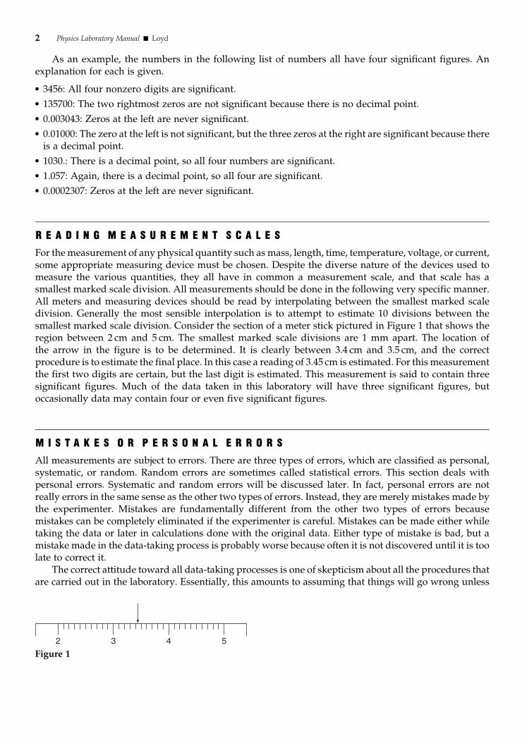
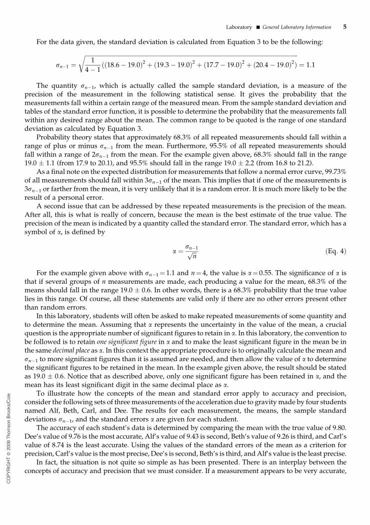
R E A D I N G M E A S U R E M E N T S C A L E SFor themeasurement of any physical quantity such as mass, length, time, temperature, voltage, or current,some appropriate measuring device must be chosen. Despite the diverse nature of the devices used tomeasure the various quantities, they all have in common a measurement scale, and that scale has asmallest marked scale division. All measurements should be done in the following very specific manner.All meters and measuring devices should be read by interpolating between the smallest marked scaledivision. Generally the most sensible interpolation is to attempt to estimate 10 divisions between thesmallest marked scale division. Consider the section of a meter stick pictured in Figure 1 that shows theregion between 2 cm and 5 cm. The smallest marked scale divisions are 1 mm apart. The location ofthe arrow in the figure is to be determined. It is clearly between 3.4 cm and 3.5 cm, and the correctprocedure is to estimate the final place. In this case a reading of 3.45 cm is estimated. For this measurementthe first two digits are certain, but the last digit is estimated. This measurement is said to contain threesignificant figures. Much of the data taken in this laboratory will have three significant figures, butoccasionally data may contain four or even five significant figures.
M I S T A K E S O R P E R S O N A L E R R O R SAll measurements are subject to errors. There are three types of errors, which are classified as personal,systematic, or random. Random errors are sometimes called statistical errors. This section deals withpersonal errors. Systematic and random errors will be discussed later. In fact, personal errors are notreally errors in the same sense as the other two types of errors. Instead, they are merely mistakes made bythe experimenter. Mistakes are fundamentally different from the other two types of errors becausemistakes can be completely eliminated if the experimenter is careful. Mistakes can be made either whiletaking the data or later in calculations done with the original data. Either type of mistake is bad, but amistake made in the data-taking process is probably worse because often it is not discovered until it is toolate to correct it.
The correct attitude toward all data-taking processes is one of skepticism about all the procedures thatare carried out in the laboratory. Essentially, this amounts to assuming that things will go wrong unless
2 3 4 5
Figure 1
2 Physics Laboratory Manual n Loyd
constant attention is given to making sure that no mistakes are made. For every measurement taken, allaspects of the process must be checked and rechecked. Everyone in the groupmust be convinced that theyknow exactly what is supposed to be measured, what the correct procedure is to measure it, and that thegroup is making no mistakes in carrying out that procedure.
A C C U R A C Y A N D P R E C I S I O NThe central point to experimental physical science is the measurement of physical quantities. It is assumedthat there exists a true value for any physical quantity, and the measurement process is an attempt todiscover that true value. It is expected that there will be some difference between the true value and themeasured value. The terms accuracy and precision are used to describe different aspects of the differencebetween the measured value and the true value of some quantity.
The accuracy of ameasurement is determined by how close the result of themeasurement is to the truevalue. For example, in several of the experiments, we will determine a value for the acceleration due togravity. For this case, the accuracy of the result is decided by how close it is to the true value of 9.80m/s2.For many laboratory experiments, the true value of the measured quantity is not known, and we cannotdetermine the accuracy of the experiment from the available data.
The precision of a measurement refers essentially to how many digits in the result are significant. Itindicates also how reproducible the results are when measurements of some quantity are repeated. Thesmaller the variations of the individual repeated measurements of a quantity, the more precise the quotedvalue of the measurement is considered to be. We will elaborate upon and quantify this idea about therelationship between the size of the variations in the measurements and the precision of the measurementin a later section on statistical methods.
S Y S T E M A T I C E R R O R SSystematic errors are errors that tend to be in the same direction for repeated measurements, givingresults that are either consistently above the true value or consistently below the true value. In many casessuch errors are caused by some flaw in the experimental apparatus. For example, a voltmeter could beincorrectly calibrated in such a way that it consistently gives a reading that is 80% of the true voltageacross its input terminals. It is also possible to have a voltmeter with a zero offset on its scale, which isassumed for this discussion to be 0.50 volts. In the first case, the error is a constant fraction of the truevalue (in this case, 20%), and in the second case, the error is a constant absolute voltage. Either of these is asystematic error, and the answer to the question of which one is worse depends upon themagnitude of thevoltage to be measured. If the voltage to be measured is l.00 volts, then the meter with absolute error of0.50 volts causes an error of 50%, whereas the meter with relative error causes an error of 20%. On theother hand, if the voltage to be measured is l00 volts, the meter with absolute error of 0.50 volts causesonly a 0.5% error, and the other meter still causes a 20% error, or in this case, 20 volts. If this measuredvoltage is used to calculate some other quantity, it too will show a systematic error in the results.
A second common type of systematic error is failure to consider all of the variables that are importantin the experiment. In some cases one may be aware that some other factors need to be considered, butmight not have the ability to do so quantitatively. For example, when using an air table to validateNewton’s Laws, it is common to ignore friction. This is done because friction is assumed to be small, butalso because often there is no easy way to determine its contribution. It is expected, therefore, thatneglecting friction might introduce a systematic error.
For purposes of this laboratory, the concern with systematic errors will usually be twofold—toattempt to eliminate any obvious systematic errors to the extent possible, and to attempt to identify anydata that show systematic error, and suggest possible reasonable causes for such error.
COPYRIG
HTª
2008ThomsonBrooks/Cole
Laboratory n General Laboratory Information 3

R A N D O M E R R O R SThe final class of errors is those that are produced by unpredictable and unknown variations in the totalexperimental process even when one does the experiment as carefully as is humanly possible. Thevariations caused by an observer’s inability to estimate the last digit the same way every time willdefinitely be one contribution. Other variations can be caused by fluctuations in line voltage, temperaturechanges, mechanical vibrations, or any of the many physical variations that may be inherent in theequipment or any other aspect of the measurement process. It is important to realize the followingdifference between random errors and personal and systematic errors. In principle all personal andsystematic errors can be eliminated, but there will always remain some random errors in anymeasurement. Even in principle the random errors can never be completely eliminated.
Random errors, on the other hand, can be determined in a prescribed way. It has been foundempirically that random errors often are distributed according to a particular statistical distributionfunction called the Gauss distribution function, which is also referred to as the normal error function.Random measurement errors are said to be normally distributed when a histogram of the frequencydistribution of the results of a large number of repeated measurements produces a bell-shaped curve witha peak at the mean of the measurements. The histogram of the frequency distribution is simply a graph ofthe number of times the measurements fall within a certain range versus the measured values.
M E A N A N D S T A N D A R D D E V I A T I O NAssume a series of repeated measurements is made in which there are no systematic or personal errors,and thus only random errors are present. Assume that there are nmeasurements made of some quantity x,and the ith value obtained is xi where i varies from 1 to n. If it is true that the errors are normallydistributed, statistical theory says that the mean is the best approximation to the true value. In formalmathematical terms, the mean (which has a symbol of x ) is given by the equation
x ¼ 1
n
� �Xn1
xi ðEq: 1Þ
For example, assume that four measurements are made of some quantity x, and that the four resultsare 18.6, 19.3, 17.7, and 20.4. Equation 1 is simply shorthand notation for the averaging process given by
x ¼ ð1=4Þ ð18:6þ 19:3þ 17:7þ 20:4Þ ¼ 19:0 ðEq: 2Þ
It is not surprising that the mean is the best approximation to the true value. It seems intuitivelyreasonable. We can prove mathematically that the mean is indeed the proper choice by something calledthe principle of least squares, which we state in the following way. The most probable value for somequantity determined from a series of measurements is that value that minimizes the sum of the squares ofthe deviations between the chosen value and the measured values. We can demonstrate that the properchoice to produce this minimum sum of deviations is simply the mean of the measurements. This idea canbe usefully generalized later for the case of two variables.
Statistical theory, furthermore, states that the precision of the measurement can be determined bycalculating a quantity called the standard deviation from the mean of the measurements. The symbol forstandard deviation from the mean is sn�1, and it is defined by the equation
sn�1 ¼ffiffiffiffiffiffiffiffiffiffiffiffiffiffiffiffiffiffiffiffiffiffiffiffiffiffiffiffiffiffiffiffiffiffiffiffi1
n� 1
Xn1
xi � x½ �2s
ðEq: 3Þ
4 Physics Laboratory Manual n Loyd
For the data given, the standard deviation is calculated from Equation 3 to be the following:
sn�1 ¼ffiffiffiffiffiffiffiffiffiffiffiffiffiffiffiffiffiffiffiffiffiffiffiffiffiffiffiffiffiffiffiffiffiffiffiffiffiffiffiffiffiffiffiffiffiffiffiffiffiffiffiffiffiffiffiffiffiffiffiffiffiffiffiffiffiffiffiffiffiffiffiffiffiffiffiffiffiffiffiffiffiffiffiffiffiffiffiffiffiffiffiffiffiffiffiffiffiffiffiffiffiffiffiffiffiffiffiffiffiffiffiffiffiffiffiffiffiffiffiffiffiffiffiffiffiffiffiffiffiffiffiffiffiffiffiffiffiffiffiffiffiffiffiffiffiffiffi1
4� 1ðð18:6� 19:0Þ2 þ ð19:3� 19:0Þ2 þ ð17:7� 19:0Þ2 þ ð20:4� 19:0Þ2Þ
r¼ 1:1
The quantity sn�1, which is actually called the sample standard deviation, is a measure of theprecision of the measurement in the following statistical sense. It gives the probability that themeasurements fall within a certain range of the measured mean. From the sample standard deviation andtables of the standard error function, it is possible to determine the probability that the measurements fallwithin any desired range about the mean. The common range to be quoted is the range of one standarddeviation as calculated by Equation 3.
Probability theory states that approximately 68.3% of all repeated measurements should fall within arange of plus or minus sn�1 from the mean. Furthermore, 95.5% of all repeated measurements shouldfall within a range of 2sn�1 from the mean. For the example given above, 68.3% should fall in the range19.0 � 1.1 (from 17.9 to 20.1), and 95.5% should fall in the range 19.0 � 2.2 (from 16.8 to 21.2).
As a final note on the expected distribution for measurements that follow a normal error curve, 99.73%of all measurements should fall within 3sn�1 of the mean. This implies that if one of the measurements is3sn�1 or farther from the mean, it is very unlikely that it is a random error. It is much more likely to be theresult of a personal error.
A second issue that can be addressed by these repeated measurements is the precision of the mean.After all, this is what is really of concern, because the mean is the best estimate of the true value. Theprecision of the mean is indicated by a quantity called the standard error. The standard error, which has asymbol of a, is defined by
a ¼ sn�1ffiffiffin
p ðEq: 4Þ
For the example given above with sn�1¼ 1.1 and n¼ 4, the value is a¼ 0.55. The significance of a isthat if several groups of n measurements are made, each producing a value for the mean, 68.3% of themeans should fall in the range 19.0 � 0.6. In other words, there is a 68.3% probability that the true valuelies in this range. Of course, all these statements are valid only if there are no other errors present otherthan random errors.
In this laboratory, students will often be asked to make repeated measurements of some quantity andto determine the mean. Assuming that a represents the uncertainty in the value of the mean, a crucialquestion is the appropriate number of significant figures to retain in a. In this laboratory, the convention tobe followed is to retain one significant figure in a and to make the least significant figure in the mean be inthe same decimal place as a. In this context the appropriate procedure is to originally calculate themean andsn�1 to more significant figures than it is assumed are needed, and then allow the value of a to determinethe significant figures to be retained in the mean. In the example given above, the result should be statedas 19.0 � 0.6. Notice that as described above, only one significant figure has been retained in a, and themean has its least significant digit in the same decimal place as a.
To illustrate how the concepts of the mean and standard error apply to accuracy and precision,consider the following sets of threemeasurements of the acceleration due to gravitymade by four studentsnamed Alf, Beth, Carl, and Dee. The results for each measurement, the means, the sample standarddeviations sn�1, and the standard errors a are given for each student.
The accuracy of each student’s data is determined by comparing the mean with the true value of 9.80.Dee’s value of 9.76 is the most accurate, Alf’s value of 9.43 is second, Beth’s value of 9.26 is third, and Carl’svalue of 8.74 is the least accurate. Using the values of the standard errors of the mean as a criterion forprecision, Carl’s value is themost precise, Dee’s is second, Beth’s is third, andAlf’s value is the least precise.
In fact, the situation is not quite so simple as has been presented. There is an interplay between theconcepts of accuracy and precision that we must consider. If a measurement appears to be very accurate,
COPYRIG
HTª
2008ThomsonBrooks/Cole
Laboratory n General Laboratory Information 5
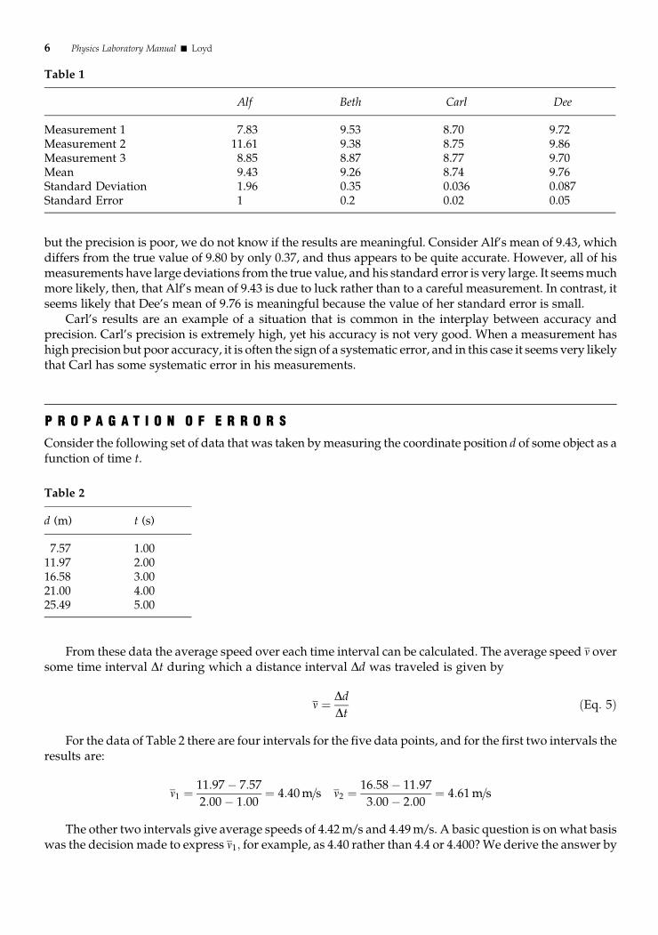
but the precision is poor, we do not know if the results are meaningful. Consider Alf’s mean of 9.43, whichdiffers from the true value of 9.80 by only 0.37, and thus appears to be quite accurate. However, all of hismeasurements have large deviations from the true value, andhis standard error is very large. It seemsmuchmore likely, then, that Alf’s mean of 9.43 is due to luck rather than to a careful measurement. In contrast, itseems likely that Dee’s mean of 9.76 is meaningful because the value of her standard error is small.
Carl’s results are an example of a situation that is common in the interplay between accuracy andprecision. Carl’s precision is extremely high, yet his accuracy is not very good. When a measurement hashigh precision but poor accuracy, it is often the sign of a systematic error, and in this case it seems very likelythat Carl has some systematic error in his measurements.
P R O P A G A T I O N O F E R R O R SConsider the following set of data that was taken bymeasuring the coordinate position d of some object as afunction of time t.
From these data the average speed over each time interval can be calculated. The average speed n oversome time interval Dt during which a distance interval Dd was traveled is given by
n ¼ DdDt
ðEq: 5Þ
For the data of Table 2 there are four intervals for the five data points, and for the first two intervals theresults are:
n1 ¼ 11:97� 7:57
2:00� 1:00¼ 4:40m=s n2 ¼ 16:58� 11:97
3:00� 2:00¼ 4:61m=s
The other two intervals give average speeds of 4.42m/s and 4.49m/s. A basic question is onwhat basiswas the decision made to express n1; for example, as 4.40 rather than 4.4 or 4.400?We derive the answer by
Table 1
Alf Beth Carl Dee
Measurement 1 7.83 9.53 8.70 9.72Measurement 2 11.61 9.38 8.75 9.86Measurement 3 8.85 8.87 8.77 9.70Mean 9.43 9.26 8.74 9.76Standard Deviation 1.96 0.35 0.036 0.087Standard Error 1 0.2 0.02 0.05
Table 2
d (m) t (s)
7.57 1.0011.97 2.0016.58 3.0021.00 4.0025.49 5.00
6 Physics Laboratory Manual n Loyd
further extending the rules for significant figures to include calculations. Use the following rules todetermine the number of significant figures to retain at the end of a calculation:
. When adding or subtracting, figures to the right of the last column in which all figures are significantshould be dropped.
. When multiplying or dividing, retain only as many significant figures in the result as are contained inthe least precise quantity in the calculation.
. The last significant figure is increased by 1 if the figure beyond it (which is dropped) is 5 or greater.
These rules apply only to the determination of the number of significant figures in the final result.In the intermediate steps of a calculation, one more significant figure should be kept than is kept in thefinal result.
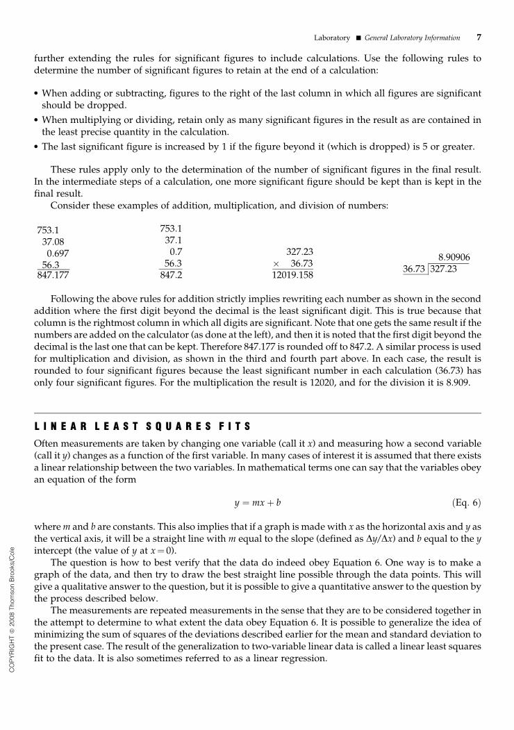
Consider these examples of addition, multiplication, and division of numbers:
753:137:080:69756:3847:177
753:137:10:7
56:3847:2
327:23� 36:7312019:158
8:9090636:73 327:23
Following the above rules for addition strictly implies rewriting each number as shown in the secondaddition where the first digit beyond the decimal is the least significant digit. This is true because thatcolumn is the rightmost column in which all digits are significant. Note that one gets the same result if thenumbers are added on the calculator (as done at the left), and then it is noted that the first digit beyond thedecimal is the last one that can be kept. Therefore 847.177 is rounded off to 847.2. A similar process is usedfor multiplication and division, as shown in the third and fourth part above. In each case, the result isrounded to four significant figures because the least significant number in each calculation (36.73) hasonly four significant figures. For the multiplication the result is 12020, and for the division it is 8.909.
L I N E A R L E A S T S Q U A R E S F I T SOften measurements are taken by changing one variable (call it x) and measuring how a second variable(call it y) changes as a function of the first variable. In many cases of interest it is assumed that there existsa linear relationship between the two variables. In mathematical terms one can say that the variables obeyan equation of the form
y ¼ mxþ b ðEq: 6Þ
wherem and b are constants. This also implies that if a graph is made with x as the horizontal axis and y asthe vertical axis, it will be a straight line with m equal to the slope (defined as Dy/Dx) and b equal to the yintercept (the value of y at x¼ 0).
The question is how to best verify that the data do indeed obey Equation 6. One way is to make agraph of the data, and then try to draw the best straight line possible through the data points. This willgive a qualitative answer to the question, but it is possible to give a quantitative answer to the question bythe process described below.
The measurements are repeated measurements in the sense that they are to be considered together inthe attempt to determine to what extent the data obey Equation 6. It is possible to generalize the idea ofminimizing the sum of squares of the deviations described earlier for the mean and standard deviation tothe present case. The result of the generalization to two-variable linear data is called a linear least squaresfit to the data. It is also sometimes referred to as a linear regression.
COPYRIG
HTª
2008ThomsonBrooks/Cole
Laboratory n General Laboratory Information 7

The aim of the process is to determine the values ofm and b that produce the best straight-line fit to thedata. Any choice of values for m and b will produce a straight line, with values of y determined by thechoice of x. For any such straight line (determined by a given m and b) there will be a deviation betweeneach of the measured y’s and the y’s from the straight-line fit at the value of the measured x’s. The leastsquares fit is that m and b for which the sum of the squares of these deviations is a minimum. Statisticaltheory states that the appropriate values ofm and b that will produce this minimum sum of squares of thedeviations are given by the following equations:
m ¼nXn1
xiyi �Xn1
xi
! Xn1
yi
!
nXn1
x2i �Xn1
xi
!2ðEq: 7Þ
b ¼
Xn1
yi
! Xn1
x2i
!�
Xn1
xiyi
! Xn1
xi
!
nXn1
x2i �Xn1
xi
!2ðEq: 8Þ
Refer again to the data of Table 2 for coordinate position versus time. The question to be answered iswhether or not the data are consistent with constant velocity. If the speed v is constant, the data can be fitby an equation of the form
d ¼ ntþ do ðEq: 9Þ
Equation 9 is of the form of Equation 6with d corresponding to y, t corresponding to x, v correspondingtom, and do corresponding to b. Thus vwill be the slope of a graph of d versus t, and dowill be the intercept,which is the coordinate position at the arbitrarily chosen time t¼ 0.
Calculating some of the individual terms gives:
Pti ¼ 1:00þ 2:00þ 3:00þ 4:00þ 5:00 ¼ 15:00P ðtiÞ2 ¼ ð1:00Þ2þð2:00Þ2þð3:00Þ2þð4:00Þ2þð5:00Þ2¼ 55:00Pdi ¼ 7:57þ 11:97þ 16:58þ 21:00þ 25:49 ¼ 82:61Ptidi ¼ ð1:00Þð7:57Þ þ ð2:00Þð11:97Þ þ ð3:00Þð16:58Þ þ ð4:00Þð21:00Þ þ ð5:00Þð25:49Þ ¼ 292:70P ðdiÞ2 ¼ ð7:57Þ2þð11:97Þ2þð16:58Þ2þð21:00Þ2þð25:49Þ2¼ 1566:22
Using these values in Equations 7 and 8 with the appropriate correspondence of variables givesv¼ 4.49 and do¼ 3.06. Thus the velocity is determined to be 4.49m/s, and the coordinate at t¼ 0 is found tobe 3.06m.
At this point, the best possible straight-line fit to the data has been determined by the least squares fitprocess. A second goal remains, to determine how well the data actually fit the straight line that we haveobtained. Again, we derive a qualitative answer to this question by making a graph of the data and thestraight line and qualitatively judging the agreement between the line and the data.
There is, however, a quantitative measure of howwell the data follow the straight line obtained by theleast squares fit. It is given by the value of a quantity called the correlation coefficient, r. This quantity is ameasure of the fit of the data to a straight line with r¼ 1.000 exactly signifying a perfect correlation, andr¼ 0 signifying no correlation at all. The equation to calculate r in terms of the general variables x and y isgiven by
8 Physics Laboratory Manual n Loyd
COPYRIG
HTª
2008ThomsonBrooks/Cole
r ¼nXn1
xiyi �Xn1
xi
! Xn1
yi
!ffiffiffiffiffiffiffiffiffiffiffiffiffiffiffiffiffiffiffiffiffiffiffiffiffiffiffiffiffiffiffiffiffiffiffiffiffiffiffiffiffiffinXn1
x2i �Xn1
xi
!2vuut
ffiffiffiffiffiffiffiffiffiffiffiffiffiffiffiffiffiffiffiffiffiffiffiffiffiffiffiffiffiffiffiffiffiffiffiffiffiffiffiffiffiffinXn1
y2i �Xn1
yi
!2vuut
ðEq: 10Þ
Making the substitutions for the variables of the problem of the fit to the displacement versus time bysubstituting t for x and d for y in the above equation and using the appropriate numerical values calculatedearlier gives r¼ 0.99998. Thus the data show an almost perfect linear relationship because r is so close to1.000. In calculations of r keep either three significant figures, or else enough until the last place is not a 9.
When performing a least squares fit to data, particularly when a small number of data points areinvolved, there is some tendency to obtain a surprisingly good value for r even for data that do notappear to be very linear. For those cases, we can determine the significance of a given value of r bycomparing the obtained value of rwith the probability that that value of rwould be obtained for n valuesof two variables that are unrelated. A table for such comparisons is given in Appendix I in a table entitledCorrelation Coefficients.
S T A T I S T I C A L C A L C U L A T I O N SA very high percentage of the laboratories in this course will involve two variables that are linearlyrelated. These cases usually will require a least squares fit to the data. Although the least squares fitcalculations and mean and standard deviation calculations are not difficult in principle, they are tediousand time-consuming. The use of a spreadsheet computer program such as Excel is highly recommended.As an alternative, many handheld calculators have automatic routines built in that allow the calculation ofthese quantities simply by inputting the data points one after another. Note that most calculators willcalculate two different standard deviations. The one needed is usually denoted sn�1, and it is the samplestandard deviation. Also available onmost calculators is a quantity that is usually denoted as sn. It appliesto the case when the population is known, and it will never be appropriate for data taken in thislaboratory. Always be sure to choose the quantity sn�1, which is the one defined by Equation 3.
P E R C E N T A G E E R R O R A N D P E R C E N T A G E D I F F E R E N C EIn several of the laboratory exercises, the true value of the quantity being measured will be considered tobe known. In those cases, the accuracy of the experiment will be determined by comparing theexperimental result with the known value. Normally this will be done by calculating the percentage errorof your measurement compared to the given known value. If E stands for the experimental value, and Kstands for the known value, then the percentage error is given by
Percentage error ¼ jE� KjK
� 100% ðEq: 11Þ
In other cases we will measure a given quantity by two different methods. There will then be twodifferent experimental values, E1 and E2, but the true value may not be known. For this case, we willcalculate the percentage difference between the two experimental values. Note that this tells nothingabout the accuracy of the experiment, but will be a measure of the precision. The percentage differencebetween the two measurements is defined as
Percentage difference ¼ jE2 � E1j½E1 þ E2�=2� 100% ðEq: 12Þ
Laboratory n General Laboratory Information 9

P R E P A R I N G G R A P H SIt is helpful to represent data in the form of a graph when interpreting the overall trend of the data. Mostof the graphs for this laboratory will use rectangular Cartesian coordinates. Note that it is customary todenote the horizontal axis as x and the vertical axis as ywhen developing general equations, as was donein the development of the equations for a linear least squares fit. However, any two variables can beplotted against each other.
When preparing a graph, first choose a scale for each of the axes. It is not necessary to choose the samescale for both axes. In fact, rarely will it be convenient to have the same scale for both axes. Instead, choosethe scale for each axis so that the graph will range over as much of the graph paper as possible, consistentwith a convenient scale. Choose scales that have the smallest divisions of the graph paper equal tomultiples of 2, 5, or 10 units. This makes it much easier to interpolate between the divisions to locate thedata points when graphing.
The student is expected to bring to each laboratory a supply of good quality linear graph paper.A very good grade of centimeter by centimeter graph paper with one division per millimeter is the bestchoice. Do not, for example, ever use 1/4 inch by 1/4 inch sketch paper or other such coarse scaled paper asgraph paper. In some cases special graph paper like semilog or log-log graph paper may be required.
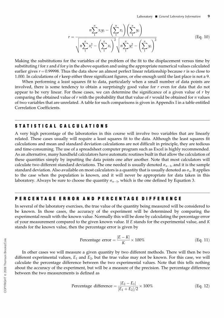
Figure 2 is a graph of the data for displacement versus time from Table 2 for which the least squares fitwas previouslymade.Note that scales for each axis have been chosen, to spread the graph over a reasonableportion of the page. Also note that because the data have been assumed linear, a straight line has beendrawn through the data points. The straight line is the one obtained from the least squares fit to the data.
For most experiments, the variables will take on only positive values. For that case the scales shouldrange from zero to greater than the largest value for any data point. For example, in Figure 2 thedisplacement is chosen to range from 0 to 30meters because the largest displacement is 25.49, and the timescale has been chosen to range from 0 to 6 seconds because the largest time is 5.00 seconds. Also note thatthe scales should not be suppressed as a means to stretch out the graph. For example, if a set of datacontains ordinates that range from 60 to 90, do not choose a scale that shows only that range. Instead ascale from 0 to 100 should be chosen, and there is nothing that can be done in that case to make the graphrange over more than about 30% of the graph paper. Scales should always be chosen to increase to theright of the origin and to increase above the origin.
00 1 2 3
Time (s)
Graph of Displacement Versus Time
4 5 6
5
10
15
20
25
30
Dis
plac
emen
t (m
)
Figure 2
10 Physics Laboratory Manual n Loyd

Graphs should always have the scales labeled with the name and units of each variable along eachaxis. Major scale divisions should be labeled with the appropriate numbers defining the scale. Alwaysinclude a title for each graph, keeping in mind that it is customary to state the vertical axis versus thehorizontal axis.
All graphs should be plotted as points with no attempt to connect the data with a smooth curve. Donot write the coordinates on the graph next to the data point, as is common practice in mathematicsclasses. The only time it is appropriate to draw any continuous line to represent the trend of the data iswhen it is assumed that the mathematical form of the data is known. In practice, the only time this will betrue will be when linearity is assumed, and in that case, it is appropriate to draw the straight line that hasbeen obtained by the least squares fitting procedure.
COPYRIG
HTª
2008ThomsonBrooks/Cole
Laboratory n General Laboratory Information 11

This page intentionally left blank

Measurement of Length
O B J E C T I V E So Demonstrate the specific knowledge gained by repeated measurements of the length and width
of a table.
o Apply the statistical concepts of mean, standard deviation from the mean, and standard error tothese measurements.
o Demonstrate propagation of errors by determining the uncertainty in the area calculated fromthe measured length and width.
E Q U I P M E N T L I S T. 2-meter stick
. Laboratory table
T H E O R YIn this laboratory it is assumed that the uncertainty in the measurement of the length and width of thetable is due to random errors. If this assumption is valid, then the mean of a series of repeated measu-rements represents the most probable value for the length or width.
Consider the general case in which n measurements of the length and width of the table are made.Wewill make 10 measurements, so n= 10 for this case, but we will develop equations for the case in whichn can be any chosen value. If Li and Wi stand for the individual measurements of the length and width,and L and W stand for the mean of those measurements, the equations relating them are
L ¼� 1n
�Xni
Li W ¼� 1n
�Xni
Wi ðEq: 1Þ
We get information about the precision of the measurement from the variations of the individualmeasurements using the statistical concept of the standard deviation. The values of the standarddeviation from the mean for the length and width of the table, sLn�1 and sWn�1; are given by the equations:
sLn�1 ¼ffiffiffiffiffiffiffiffiffiffiffiffiffiffiffiffiffiffiffiffiffiffiffiffiffiffiffiffiffiffiffiffiffiffiffiffiffi1
n� 1
Xn1
ðLi � LÞ2s
sWn�1 ¼ffiffiffiffiffiffiffiffiffiffiffiffiffiffiffiffiffiffiffiffiffiffiffiffiffiffiffiffiffiffiffiffiffiffiffiffiffiffiffiffiffi1
n� 1
Xn1
ðWi �WÞ2s
ðEq: 2Þ
Physics Laboratory Manual n Loyd L A B O R A T O R Y 1
COPYRIG
HTª
2008ThomsonBrooks/Cole
13
ª 2008 Thomson Brooks/Cole, a part of TheThomson Corporation.Thomson, the Star logo, and Brooks/Cole are trademarks used herein under license. ALL RIGHTSRESERVED.No part of this workcovered by the copyright hereonmay be reproduced or used in any form or by any meansçgraphic, electronic, ormechanical, including photocopying, recording, taping,web distribution, informationstorage and retrieval systems,or in any othermannerçwithout the written permission of the publisher.

If errors are only random, it should be true that approximately 68.3% of the measurements of lengthshould fall in the range L � sLn�1; and that approximately 68.3% of the measurements of width should fallwithin the range W � sWn�1: Furthermore, 95.5% of the measurements of both length and width shouldfall within 2 sn–1 of the mean, and 99.73% should fall within 3 sn–1 of the mean.
The precision of the mean for L and W is given by quantities called the standard error, aL and aW.These quantities are defined by the following equations:
aL ¼ sLn�1ffiffiffin
p aW ¼ sWn�1ffiffiffin
p ðEq: 3Þ
The meaning of aL and aW is that, if the errors are only random, there is a 68.3% chance that the true valueof the length lies within the range L� aL and the true value of the width lies within the range W � aW .
An important problem in experimental physics is to determine the uncertainty in some quantitythat is derived by calculations from other directly measured quantities. For this experiment, consider thearea A of the table as calculated from the measured values of the length and width L and W by thefollowing:
A ¼ L � W ðEq: 4Þ
For the case of an area that is the product of twomeasured quantities, the uncertainty in the area is relatedto the uncertainty of the length and width by:
aA ¼ffiffiffiffiffiffiffiffiffiffiffiffiffiffiffiffiffiffiffiffiffiffiffiffiffiffiffiffiffiffiffiffiffiffiffiffiffiffiffiffiffiffiffiffiffiffiffiðLÞ2ðaWÞ2 þ ðWÞ2ðaLÞ2
qðEq: 5Þ
E X P E R I M E N T A L P R O C E D U R E1. Place the 2-meter stick along the length of the table near the middle of the width and parallel to one
edge of the length. Do not attempt to line up either edge of the table with one end of the meter stick orwith any certain mark on the meter stick.
2. Let X stand for the coordinate position in the length direction. Read the scale on the 2-meter stick thatis aligned with one end of the table and record that measurement in Data and Calculations Table 1 asX1. Read the scale that is aligned at the other end of the table and record that measurement in Data andCalculations Table 1 as X2. A 3�5 note card held next to the edge of the table may help to determinewhere the 2-meter stick is aligned with the table for each measurement. Note that the stick has1 millimeter as the smallest marked scale division. Therefore, each coordinate should be estimated to thenearest 0.1 millimeter (nearest 0.0001 m).
3. Repeat Steps 1 and 2 nine more times for a total of 10 measurements of the length of the table. For eachmeasurement place the 2-meter stick on the table with no attempt to align either end of the stick or anyparticular mark on the stick with either end of the table. Make the measurements at 10 differentplaces along the width of the table so that any variation in the length of the table is included in themeasurements.
4. Perform Steps 1 through 3 for 10 measurements of the width of the table. Let the coordinate for thewidth be given by Y and record the 10 values of Y1 and Y2 in Data and Calculations Table 2. Againplace the stick along the different lines each time, but make no attempt to align any particular mark onthe stick with either edge of the table.
14 Physics Laboratory Manual n Loyd

C A L C U L A T I O N S1. After all measurements are completed, perform the subtractions of the coordinate positions to
determine the 10 values of the length Li, and the 10 values of widthWi. Record the 10 values of Li andWi in the appropriate table.
2. Use Equations 1 to calculate the mean length L and the mean width W and record their values in theappropriate table. Keep five decimal places in these results. For example, typical values might beL ¼ 1:37157m and W ¼ 0:76384m.
3. For each measurement of length and width, calculate the values of Li � L andWi �W and record themin the appropriate table. Then for each value of the length and width, calculate and record the valuesof ðLi �LÞ2 and ðWi �WÞ2 in the appropriate table.
4. Perform the summations of the values of ðLi� LÞ2 and the summations of the values of ðWi �WÞ2 andrecord them in the appropriate box in the tables.
5. Use the values of the summations of ðLi � LÞ2 and of ðWi �WÞ2 in Equations 2 to calculate the values ofsLn�1 and sWn�1 and record them in the appropriate table.
6. Calculate L� sLn�1; Lþ sLn�1; W � sWn�1; and W þ sWn�1 and record the values in the appropriate table.
7. Use the values of sLn�1 and sWn�1 in Equations 3 to calculate the values of aL and aW and record them inthe appropriate table.
8. Use the values of L andW in Equation 4 to calculate the value of A, the area of the table, and record itin the appropriate table. Use Equation 5 to calculate the value of aA and record it in the appropriatetable.
COPYRIG
HTª
2008ThomsonBrooks/Cole
Laboratory 1 n Measurement of Length 15

This page intentionally left blank
Name . . . . . . . . . . . . . . . . . . . . . . . . . . . . . . . . . . . . . . . . . . . . . . . . . . . . . . . . . . . . . . . . . . . . . . . . . Section . . . . . . . . . . . . . . . . Date . . . . . . . . . . . . . . . .
1 L A B O R A T O R Y 1 Measurement of Length
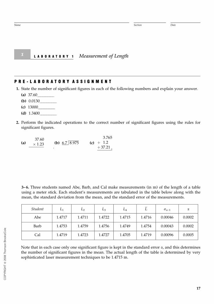
P R E - L A B O R A T O R Y A S S I G N M E N T1. State the number of significant figures in each of the following numbers and explain your answer.
(a) 37.60__________
(b) 0.0130__________
(c) 13000__________
(d) 1.3400__________
2. Perform the indicated operations to the correct number of significant figures using the rules forsignificant figures.
(a)37:60
� 1:23 (b) 6:7 j 8:975 (c)
3:765þ 1:2þ 37:21
3–6. Three students named Abe, Barb, and Cal make measurements (in m) of the length of a tableusing a meter stick. Each student’s measurements are tabulated in the table below along with themean, the standard deviation from the mean, and the standard error of the measurements.
Student L1 L2 L3 L4 L sn–1 a
Abe 1.4717 1.4711 1.4722 1.4715 1.4716 0.00046 0.0002
Barb 1.4753 1.4759 1.4756 1.4749 1.4754 0.00043 0.0002
Cal 1.4719 1.4723 1.4727 1.4705 1.4719 0.00096 0.0005
Note that in each case only one significant figure is kept in the standard error a, and this determinesthe number of significant figures in the mean. The actual length of the table is determined by verysophisticated laser measurement techniques to be 1.4715 m.
COPYRIG
HTª
2008ThomsonBrooks/Cole
17
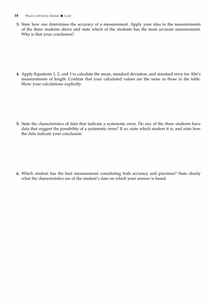
3. State how one determines the accuracy of a measurement. Apply your idea to the measurementsof the three students above and state which of the students has the most accurate measurement.Why is that your conclusion?
4. Apply Equations 1, 2, and 3 to calculate the mean, standard deviation, and standard error for Abe’smeasurements of length. Confirm that your calculated values are the same as those in the table.Show your calculations explicitly.
5. State the characteristics of data that indicate a systematic error. Do any of the three students havedata that suggest the possibility of a systematic error? If so, state which student it is, and state howthe data indicate your conclusion.
6. Which student has the best measurement considering both accuracy and precision? State clearlywhat the characteristics are of the student’s data on which your answer is based.
18 Physics Laboratory Manual n Loyd

Name . . . . . . . . . . . . . . . . . . . . . . . . . . . . . . . . . . . . . . . . . . . . . . . . . . . . . . . . . . . . . . . . . . . . . . . . . Section . . . . . . . . . . . . . . . . Date . . . . . . . . . . . . . . . .
Lab Partners . . . . . . . . . . . . . . . . . . . . . . . . . . . . . . . . . . . . . . . . . . . . . . . . . . . . . . . . . . . . . . . . . . . . . . . . . . . . . . . . . . . . . . . . . . . . . . . . . . . . . . . . . . . . . . . . . . . .
1 L A B O R A T O R Y 1 Measurement of Length
L A B O R A T O R Y R E P O R T
COPYRIG
HTª
2008ThomsonBrooks/Cole
Data and Calculations Table 1 (nearest 0.0001 m, which is 0.1 mm)
Trial X1 (m) X2 (m) Li =X2 –X1 (m) Li � L (m) ðLi � LÞ2 (m2)
Xn1
ðLi � LÞ2 ¼
L ¼ sLn�1 ¼ L� sLn�1 ¼ Lþ sLn�1 ¼ aL ¼
19
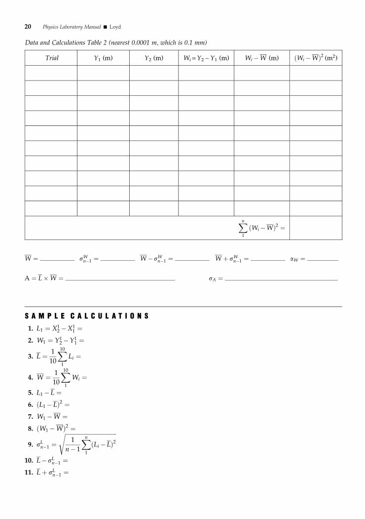
S A M P L E C A L C U L A T I O N S1. L1 ¼ X1
2 �X11 ¼
2. W1 ¼ Y12 �Y1
1 ¼
3. L ¼ 1
10
X101
Li ¼
4. W ¼ 1
10
X101
Wi ¼
5. L1 � L ¼6. ðL1 � LÞ2 ¼7. W1 �W ¼8. ðW1 �WÞ2 ¼
9. sLn�1 ¼ffiffiffiffiffiffiffiffiffiffiffiffiffiffiffiffiffiffiffiffiffiffiffiffiffiffiffiffiffiffiffiffiffiffiffiffi1
n� 1
Xn1
ðLi � LÞ2s
10. L� sLn�1 ¼11. Lþ sLn�1 ¼
Data and Calculations Table 2 (nearest 0.0001 m, which is 0.1 mm)
Trial Y1 (m) Y2 (m) Wi=Y2 – Y1 (m) Wi �W (m) ðWi �WÞ2 (m2)
Xn1
ðWi �WÞ2 ¼
W ¼ sWn�1 ¼ W � sWn�1 ¼ W þ sWn�1 ¼ aW ¼
A ¼ L�W ¼ sA ¼
20 Physics Laboratory Manual n Loyd
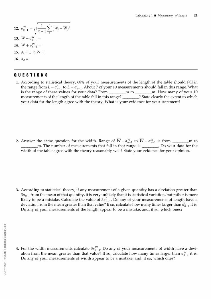
12. sWn�1 ¼ffiffiffiffiffiffiffiffiffiffiffiffiffiffiffiffiffiffiffiffiffiffiffiffiffiffiffiffiffiffiffiffiffiffiffiffiffiffiffiffi1
n� 1
Xn1
ðWi �WÞ2s
13. W � sWn�1 ¼14. W þ sWn�1 ¼15. A ¼ L�W ¼16. sA=
Q U E S T I O N S1. According to statistical theory, 68% of your measurements of the length of the table should fall in
the range from L� sLn�1 to Lþ sLn�1. About 7 of your 10 measurements should fall in this range. Whatis the range of these values for your data? From __________m to __________m. How many of your 10measurements of the length of the table fall in this range? __________? State clearly the extent to whichyour data for the length agree with the theory. What is your evidence for your statement?
2. Answer the same question for the width. Range of W � sWn�1 to W þ sWn�1 is from __________m to__________m. The number of measurements that fall in that range is __________. Do your data for thewidth of the table agree with the theory reasonably well? State your evidence for your opinion.
3. According to statistical theory, if any measurement of a given quantity has a deviation greater than3sn–1 from the mean of that quantity, it is very unlikely that it is statistical variation, but rather is morelikely to be a mistake. Calculate the value of 3sLn�1. Do any of your measurements of length have adeviation from the mean greater than that value? If so, calculate howmany times larger than sLn�1 it is.Do any of your measurements of the length appear to be a mistake, and, if so, which ones?
4. For the width measurements calculate 3sWn�1. Do any of your measurements of width have a devi-ation from the mean greater than that value? If so, calculate how many times larger than sWn�1 it is.Do any of your measurements of width appear to be a mistake, and, if so, which ones?
COPYRIG
HTª
2008ThomsonBrooks/Cole
Laboratory 1 n Measurement of Length 21

5. If possible, state the accuracy of your measurements of the length and width and give your reasoning.If this cannot be done, state why it is not possible. If possible, state the precision of your measurementof the length and width and give your reasoning. If this cannot be done, state why it is not possible.
22 Physics Laboratory Manual n Loyd

Measurement of Density
O B J E C T I V E So Determine the mass, length, and diameter of three cylinders of different metals.
o Calculate the density of the cylinders and compare with the accepted values of the density of themetals.
o Determine the uncertainty in the value of the calculated density caused by the uncertainties inthe measured mass, length, and diameter.
E Q U I P M E N T L I S T. Three solid cylinders of different metals (aluminum, brass, and iron)
. Vernier calipers
. Laboratory balance and calibrated masses
T H E O R YThe most general definition of density is mass per unit volume. Density can vary throughout the body ifthe mass is not distributed uniformly. If the mass in an object is distributed uniformly throughout theobject, the density r is defined as the total massM divided by the total volume V of the object. In equationform this is
r ¼ M
VðEq: 1Þ
For a cylinder the volume is given by
V ¼ pd2L4
ðEq: 2Þ
where d is the cylinder diameter, and L is its length. Using Equation 2 in Equation 1 gives
r ¼ 4M
pd2LðEq: 3Þ
We will determine the quantities M, d, and L by measuring each of them four times and calculatingthe mean and standard error for each quantity. Using the mean of each measured quantity in Equation 3leads to the best value for the measured density r.
Physics Laboratory Manual n Loyd L A B O R A T O R Y 2
COPYRIG
HTª
2008ThomsonBrooks/Cole
23
ª 2008 Thomson Brooks/Cole, a part of TheThomson Corporation.Thomson, the Star logo, and Brooks/Cole are trademarks used herein under license. ALL RIGHTSRESERVED.No part of this workcovered by the copyright hereonmay be reproduced or used in any form or by any meansçgraphic, electronic, ormechanical, including photocopying, recording, taping,web distribution, informationstorage and retrieval systems,or in any othermannerçwithout the written permission of the publisher.

An important question in experimental physics is how the uncertainty in a quantity calculated fromother measured quantities is related to the uncertainty in those measured quantities. For this laboratory,the uncertainty in the density (standard error) is related to the standard errors in the mass, length, anddiameter by:
ar ¼ r
ffiffiffiffiffiffiffiffiffiffiffiffiffiffiffiffiffiffiffiffiffiffiffiffiffiffiffiffiffiffiffiffiffiffiffiffiffiffiffiffiffiffiffiffiffiffiðaMM
Þ2 þ ðaLLÞ2 þ 4ðad
dÞ2
rðEq: 4Þ
The form of this equation is stated here without proof, but it can be derived from the relationshipbetween the measured quantities and the density described by Equation 3.
We determine the mass of the cylinders with a laboratory balance, which balances the weight of anunknown mass m against the weight of a known mass mk. Although the balance is between two forces(the weight of the masses), the scales can be calibrated in terms of mass assuming that the force per unitmass is the same for both the known and unknown mass. The unknown mass on a pan at the left isbalanced against the sum of all the known masses placed on the right pan plus the mass equivalent ofthe permanent sliding mass on the beam. Figure 2-1 shows a picture of a Harvard Trip balance, which hasa calibrated beam along which a permanent sliding mass can be moved in units of 0.1 gram up to10 grams.
The length and diameter of the metal cylinder will be measured with a vernier caliper. A caliper isactually any device used to determine thickness, the diameter of an object, or the distance between twosurfaces. Often calipers are in the form of two legs fastened together with a rivet, so they can pivot aboutthe fastened point. The vernier caliper used in this laboratory consists of a fixed rule that contains one jaw,and a second jaw with a vernier scale that slides along the fixed rule scale as shown in Figure 2-2.Vernier is the name given to any scale that aids in interpolating between marked divisions.
24 Physics Laboratory Manual n Loyd
Image not available due to copyright restrictions
Image not available due to copyright restrictions
The caliper has marked on the main scale major divisions of 1 cm for which there are both a mark anda number. On the main scale are also marked 10 divisions, each 1mm apart between the 1 cm divisions.The 1mm marks are not labeled with a number. This vernier is marked with a scale that, when alignedwith different marks on the fixed rule scale, allows interpolation between the 1mm marks on the fixedscale to 0.1mm accurately. A vernier caliper can measure distances accurately to the nearest 0.01 cm.
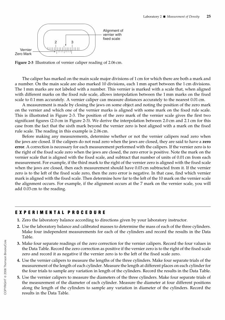
A measurement is made by closing the jaws on some object and noting the position of the zero markon the vernier and which one of the vernier marks is aligned with some mark on the fixed rule scale.This is illustrated in Figure 2-3. The position of the zero mark of the vernier scale gives the first twosignificant figures (2.0 cm in Figure 2-3). We derive the interpolation between 2.0 cm and 2.1 cm for thiscase from the fact that the sixth mark beyond the vernier zero is best aligned with a mark on the fixedrule scale. The reading in this example is 2.06 cm.
Before making any measurements, determine whether or not the vernier calipers read zero whenthe jaws are closed. If the calipers do not read zero when the jaws are closed, they are said to have a zeroerror. A correction is necessary for each measurement performed with the calipers. If the vernier zero is tothe right of the fixed scale zero when the jaws are closed, the zero error is positive. Note the mark on thevernier scale that is aligned with the fixed scale, and subtract that number of units of 0.01 cm from eachmeasurement. For example, if the third mark to the right of the vernier zero is aligned with the fixed scalewhen the jaws are closed, then each measurement should have 0.03 cm subtracted from it. If the vernierzero is to the left of the fixed scale zero, then the zero error is negative. In that case, find which verniermark is aligned with the fixed scale. Then determine how far to the left of the 10 mark on the vernier scalethe alignment occurs. For example, if the alignment occurs at the 7 mark on the vernier scale, you willadd 0.03 cm to the reading.
E X P E R I M E N T A L P R O C E D U R E1. Zero the laboratory balance according to directions given by your laboratory instructor.
2. Use the laboratory balance and calibrated masses to determine the mass of each of the three cylinders.Make four independent measurements for each of the cylinders and record the results in the DataTable.
3. Make four separate readings of the zero correction for the vernier calipers. Record the four values inthe Data Table. Record the zero correction as positive if the vernier zero is to the right of the fixed scalezero and record it as negative if the vernier zero is to the left of the fixed scale zero.
4. Use the vernier calipers to measure the lengths of the three cylinders. Make four separate trials of themeasurement of the length of each cylinder. Measure the length at different places on each cylinder forthe four trials to sample any variation in length of the cylinders. Record the results in the Data Table.
5. Use the vernier calipers to measure the diameters of the three cylinders. Make four separate trials ofthe measurement of the diameter of each cylinder. Measure the diameter at four different positionsalong the length of the cylinders to sample any variation in diameter of the cylinders. Record theresults in the Data Table.C
OPYRIG
HTª
2008ThomsonBrooks/Cole
Alignment ofvernier withfixed scale
VernierZero Mark
2 3
Figure 2-3 Illustration of vernier caliper reading of 2.06 cm.
Laboratory 2 n Measurement of Density 25

C A L C U L A T I O N S1. Calculate the mean M, the standard deviation sn–1, and the standard error aM for the four
measurements of the mass of each cylinder and record the results in the Data Table. For this and allsubsequent calculations keep one significant figure only for all standard errors, and then keep thenumber of decimal places in the mean that coincides with the decimal place of the standard error.
2. Determine the measured length and diameter for each trial by making the appropriate zero correctionto each measurement and then calculating the means L and d, the standard deviations, and thestandard errors aL and ad for each cylinder. Record the results in the Data Table.
3. Use Equation 3 to calculate the density r of each of the cylinders. Use the mean values for the mass,diameter, and length. Use Equation 4 to calculate the standard error of the density. Record the resultsin the Data Table.
4. For purposes of this laboratory, assume that the density of aluminum is 2.70 gram/cm3, the density ofbrass is 8.40 gram/cm3, and the density of iron is 7.85 gram/cm3. Calculate the percentage error inyour results for the density of each of these metals.
26 Physics Laboratory Manual n Loyd
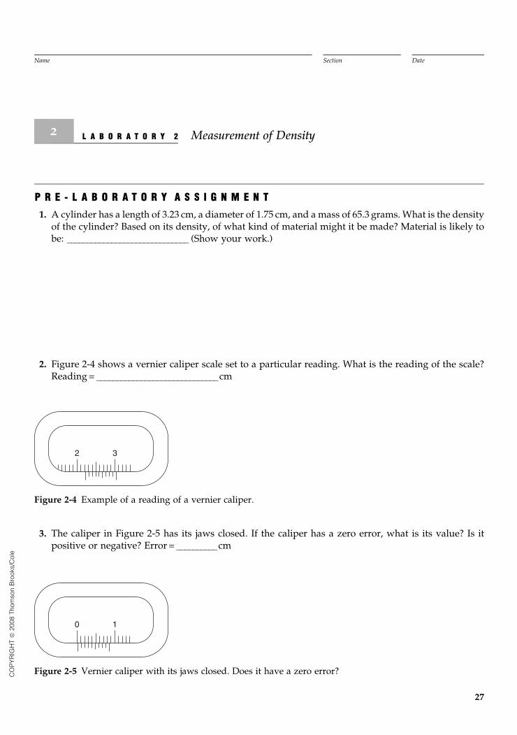
Name . . . . . . . . . . . . . . . . . . . . . . . . . . . . . . . . . . . . . . . . . . . . . . . . . . . . . . . . . . . . . . . . . . . . . . . . . Section . . . . . . . . . . . . . . . . Date . . . . . . . . . . . . . . . .
2 L A B O R A T O R Y 2 Measurement of Density
P R E - L A B O R A T O R Y A S S I G N M E N T1. A cylinder has a length of 3.23 cm, a diameter of 1.75 cm, and a mass of 65.3 grams.What is the density
of the cylinder? Based on its density, of what kind of material might it be made? Material is likely tobe: ______________________________ (Show your work.)
2. Figure 2-4 shows a vernier caliper scale set to a particular reading. What is the reading of the scale?Reading= ______________________________cm
3. The caliper in Figure 2-5 has its jaws closed. If the caliper has a zero error, what is its value? Is itpositive or negative? Error = __________cm
COPYRIG
HTª
2008ThomsonBrooks/Cole
0 1
Figure 2-5 Vernier caliper with its jaws closed. Does it have a zero error?
2 3
Figure 2-4 Example of a reading of a vernier caliper.
27
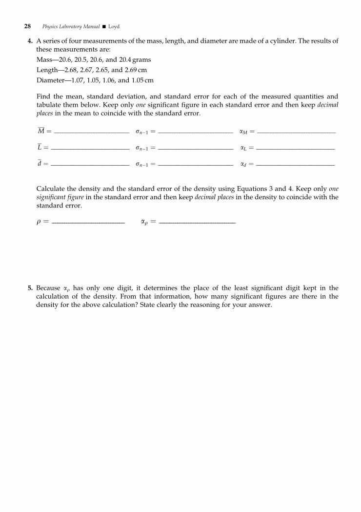
4. A series of four measurements of the mass, length, and diameter are made of a cylinder. The results ofthese measurements are:
Mass—20.6, 20.5, 20.6, and 20.4 grams
Length—2.68, 2.67, 2.65, and 2.69 cm
Diameter—1.07, 1.05, 1.06, and 1.05 cm
Find the mean, standard deviation, and standard error for each of the measured quantities andtabulate them below. Keep only one significant figure in each standard error and then keep decimalplaces in the mean to coincide with the standard error.
M ¼ sn�1 ¼ aM ¼
L ¼ sn�1 ¼ aL ¼
d ¼ sn�1 ¼ ad ¼
Calculate the density and the standard error of the density using Equations 3 and 4. Keep only onesignificant figure in the standard error and then keep decimal places in the density to coincide with thestandard error.
r ¼ ar ¼
5. Because ar has only one digit, it determines the place of the least significant digit kept in thecalculation of the density. From that information, how many significant figures are there in thedensity for the above calculation? State clearly the reasoning for your answer.
28 Physics Laboratory Manual n Loyd

Name . . . . . . . . . . . . . . . . . . . . . . . . . . . . . . . . . . . . . . . . . . . . . . . . . . . . . . . . . . . . . . . . . . . . . . . . . Section . . . . . . . . . . . . . . . . Date . . . . . . . . . . . . . . . .
Lab Partners . . . . . . . . . . . . . . . . . . . . . . . . . . . . . . . . . . . . . . . . . . . . . . . . . . . . . . . . . . . . . . . . . . . . . . . . . . . . . . . . . . . . . . . . . . . . . . . . . . . . . . . . . . . . . . . . . . . .
2 L A B O R A T O R Y 2 Measurement of Density
L A B O R A T O R Y R E P O R T
Zero Reading of the calipers ______________________________
COPYRIG
HTª
2008ThomsonBrooks/Cole
Length Data and Calculations Table
L1 (m) L2 (m) L3 (m) L4 (m) L (m) sn–1 (m) aL (m)
Aluminum
Brass
Iron
Mass Data and Calculations Table
M1 (kg) M2 (kg) M3 (kg) M4 (kg) M (kg) sn–1 (kg) aM (kg)
Aluminum
Brass
Iron
Diameter Data and Calculations Table
d1 (m) d2 (m) d3 (m) d4 (m) d (m) sn–1 (m) ad (m)
Aluminum
Brass
Iron
29
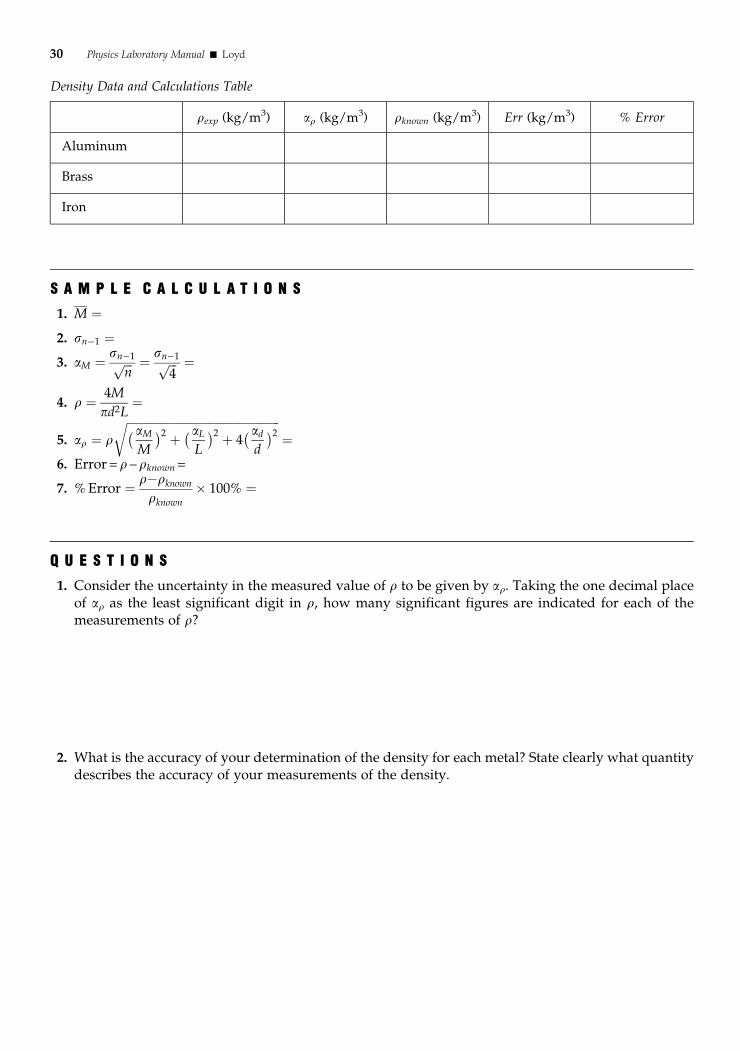
S A M P L E C A L C U L A T I O N S1. M ¼2. sn�1 ¼3. aM ¼ sn�1ffiffiffi
np ¼ sn�1ffiffiffi
4p ¼
4. r ¼ 4M
pd2L¼
5. ar ¼ r
ffiffiffiffiffiffiffiffiffiffiffiffiffiffiffiffiffiffiffiffiffiffiffiffiffiffiffiffiffiffiffiffiffiffiffiffiffiffiffiffiffiffiffiffiffiffiffiffiffiffiffiffiffi� aMM
�2 þ � aLL
�2 þ 4� add
�2r¼
6. Error =r – rknown=
7. %Error ¼ r�rknownrknown
� 100% ¼
Q U E S T I O N S1. Consider the uncertainty in the measured value of r to be given by ar. Taking the one decimal place
of ar as the least significant digit in r, how many significant figures are indicated for each of themeasurements of r?
2. What is the accuracy of your determination of the density for each metal? State clearly what quantitydescribes the accuracy of your measurements of the density.
Density Data and Calculations Table
rexp (kg/m3) ar (kg/m
3) rknown (kg/m3) Err (kg/m3) % Error
Aluminum
Brass
Iron
30 Physics Laboratory Manual n Loyd

3. Consider the value of the standard error ar as an indication of the precision of your measurements.Express the standard error as a percentage of the measured value of the density, and relate it to theaccuracy of each of your measurements.
4. Considering your answers to Question 3, is there evidence for a systematic error in any of yourmeasurements of the density of any of the metals? State clearly your evidence either for or against thepresence of a systematic error.
5. For the same percentage error in each of the three quantities, mass, diameter, and length, whichwouldcontribute the most to the error in the density? (Hint—Consider the form of Equation 4.)
COPYRIG
HTª
2008ThomsonBrooks/Cole
Laboratory 2 n Measurement of Density 31

This page intentionally left blank
Force Table and VectorAddition of Forces
O B J E C T I V E So Demonstrate the addition of several vectors to form a resultant vector using a force table.
o Demonstrate the relationship between the resultant of several vectors and the equilibrant ofthose vectors.
o Illustrate and practice graphical and analytical solutions for the addition of vectors.
E Q U I P M E N T L I S T. Force table with pulleys, ring, and string
. Mass holders and slotted masses
. Protractor and compass
T H E O R YPhysical quantities that can be completely specified by magnitude only are called scalars. Examples ofscalars include temperature, volume, mass, and time intervals. Some physical quantities have bothmagnitude and direction. These are called vectors. Examples of vector quantities include spatial dis-placement, velocity, and force.
Consider the case of several forces with different magnitudes and directions that act at the same point.The single force, which is equivalent in its effect to the effect produced by the several applied forces, iscalled the resultant force. This resultant force can be found theoretically by a special addition processknown as vector addition.
One process of vector addition is by graphical techniques. Figure 3-1(a) shows the case of two vectors,F1 of magnitude 20.0 N, and F2 of magnitude 30.0 N. A scale of 1.00 cm=10.0N is used, and these vectorsare shown as 2.00 cm and 3.00 cm in length, respectively. The forces are assumed to act at the same point,but 608 different in direction as shown. Figure 3-1(b) shows the graphical addition process called theparallelogrammethod. Two lines are constructed, each one parallel to one of the vectors having the lengthof that vector as shown. The resultant FR of the vector addition of F1 and F2 is found by constructing thestraight line from the point at the tails of the two vectors to the opposite corner of the parallelogram formedby the original vectors and the constructed lines. Ameasurement of the length of FR in Figure 3-1(b) showsit to be 4.35 cm in length, and a measurement of the angle between FR and F1 shows it to be about 378.Because the scale is 1.00 cm=10.0N, the value of the resultant FR is 43.5N, and it acts in a direction 378withrespect to the direction of F1.
Physics Laboratory Manual n Loyd L A B O R A T O R Y 3
COPYRIG
HTª
2008ThomsonBrooks/Cole
33
ª 2008 Thomson Brooks/Cole, a part of TheThomson Corporation.Thomson, the Star logo, and Brooks/Cole are trademarks used herein under license. ALL RIGHTSRESERVED.No part of this workcovered by the copyright hereonmay be reproduced or used in any form or by any meansçgraphic, electronic, ormechanical, including photocopying, recording, taping,web distribution, informationstorage and retrieval systems,or in any othermannerçwithout the written permission of the publisher.

In the graphical vector addition process known as the polygonmethod one of the vectors is first drawnto scale. Each successive vector to be added is drawn with its tail starting at the head of the precedingvector. The resultant vector is the vector drawn from the tail of the first arrow to the head of the last arrow.Figure 3-1(c) shows this process for the case of only two vectors (for which the polygon method is thetriangle method). The second vector, F2, must be drawn at the proper angle relative to F1 by extending aline in the direction of F1 and constructing F2 relative to that line. In Figure 3-1(c) the length of FR is 4.35 cmcorresponding to 43.5 N, and it acts at 378 with respect to F1.
The polygon method is illustrated for the case of three vectors in Figure 3-2. Vector F1 is drawn, F2 isdrawn at the proper angle a relative to F1, and F3 is drawn at the proper angle b relative to F2. The resultantFR is the vector connecting the tail of F1 and the head of F3.
The analytical process of vector addition uses trigonometry to express each vector in terms of itscomponents projected on the axes of a rectangular coordinate system. Figure 3-3 shows a vector, a coordinatesystem superimposed on the vector, and the components jFjcos y and jFjsin y into which the vector isresolved.When the analytical process formultiple vectors is used, each vector is resolved into components inthatmanner. The components along each axis are then added algebraically to produce the net components ofthe resultant vector along each axis. Those components are at right angles, and themagnitude of the resultantcan be found from the Pythagorean theorem. The case of three vectors, F1, F2, and F3, is shown in Figure 3-4.
60° 37° 37°
(a) (b) (c)
60°
F2 F2F2
FR � F1 � F2
FR � F1 � F2
F1 F1 F1
Figure 3-1 Illustration of the parallelogram and triangle addition of vectors.
(a) (b)
FR � F1 � F2 � F3
F2
F1 F1
F2
F3
F3
�
���
Figure 3-2 Illustration of the polygon method for vector addition.
(b)(a)
x
y
x
y
(c)
F F F sin�
F cos�
� �
Figure 3-3 Illustration of analytical resolution of a vector.
34 Physics Laboratory Manual n Loyd
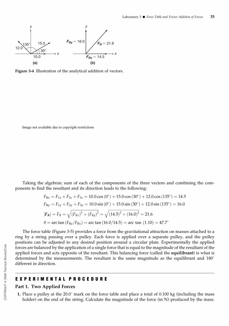
COPYRIG
HTª
2008ThomsonBrooks/Cole
Taking the algebraic sum of each of the components of the three vectors and combining the com-ponents to find the resultant and its direction leads to the following:
FRx ¼ F1x þ F2x þ F3x ¼ 10:0 cos ð0�Þ þ 15:0 cos ð30�Þ þ 12:0 cos ð135�Þ ¼ 14:5
FRy ¼ F1y þ F2y þ F3y ¼ 10:0 sin ð0�Þ þ 15:0 sin ð30�Þ þ 12:0 sin ð135�Þ ¼ 16:0
jFRj ¼ FR ¼ffiffiffiffiffiffiffiffiffiffiffiffiffiffiffiffiffiffiffiffiffiffiffiffiffiffiffiffiffiffiffiðFRxÞ2 þ ðFRyÞ2
q¼
ffiffiffiffiffiffiffiffiffiffiffiffiffiffiffiffiffiffiffiffiffiffiffiffiffiffiffiffiffiffiffiffiffiffiffið14:5Þ2 þ ð16:0Þ2
q¼ 21:6
y ¼ arc tan ðFRy=FRxÞ ¼ arc tan ð16:0=14:5Þ ¼ arc tan ð1:10Þ ¼ 47:7�
The force table (Figure 3-5) provides a force from the gravitational attraction on masses attached to aring by a string passing over a pulley. Each force is applied over a separate pulley, and the pulleypositions can be adjusted to any desired position around a circular plate. Experimentally the appliedforces are balanced by the application of a single force that is equal to the magnitude of the resultant of theapplied forces and acts opposite of the resultant. This balancing force (called the equilibrant) is what isdetermined by the measurements. The resultant is the same magnitude as the equilibrant and 1808different in direction.
E X P E R I M E N T A L P R O C E D U R EPart 1. Two Applied Forces
1. Place a pulley at the 20.08 mark on the force table and place a total of 0.100 kg (including the massholder) on the end of the string. Calculate the magnitude of the force (in N) produced by the mass.
12.015.0
y y
x x10.0
(a) (b)
135°
30°
FRy � 16.0
FRx � 14.5
FR � 21.6
Figure 3-4 Illustration of the analytical addition of vectors.
Laboratory 3 n Force Table and Vector Addition of Forces 35
Image not available due to copyright restrictions
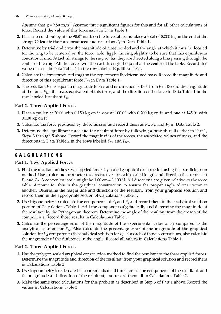
Assume that g = 9.80 m/s2. Assume three significant figures for this and for all other calculations offorce. Record the value of this force as F1 in Data Table 1.
2. Place a second pulley at the 90.08mark on the force table and place a total of 0.200 kg on the end of thestring. Calculate the force produced and record as F2 in Data Table 1.
3. Determine by trial and error the magnitude of mass needed and the angle at which it must be locatedfor the ring to be centered on the force table. Jiggle the ring slightly to be sure that this equilibriumcondition is met. Attach all strings to the ring so that they are directed along a line passing through thecenter of the ring. All the forces will then act through the point at the center of the table. Record thisvalue of mass in Data Table 1 in the row labeled Equilibrant FE1.
4. Calculate the force produced (mg) on the experimentally determinedmass. Record themagnitude anddirection of this equilibrant force FE1 in Data Table 1.
5. The resultant FR1 is equal in magnitude to FE1, and its direction is 1808 from FE1. Record the magnitudeof the force FR1, the mass equivalent of this force, and the direction of the force in Data Table 1 in therow labeled Resultant FR1.
Part 2. Three Applied Forces
1. Place a pulley at 30.08 with 0.150 kg on it, one at 100.08 with 0.200 kg on it, and one at 145.08 with0.100 kg on it.
2. Calculate the force produced by those masses and record them as F3, F4, and F5 in Data Table 2.
3. Determine the equilibrant force and the resultant force by following a procedure like that in Part 1,Steps 3 through 5 above. Record the magnitudes of the forces, the associated values of mass, and thedirections in Data Table 2 in the rows labeled FE2 and FR2.
C A L C U L A T I O N SPart 1. Two Applied Forces
1. Find the resultant of these two applied forces by scaled graphical construction using the parallelogrammethod. Use a ruler and protractor to construct vectors with scaled length and direction that representF1 and F2. A convenient scale might be 1.00 cm=0.100N. All directions are given relative to the forcetable. Account for this in the graphical construction to ensure the proper angle of one vector toanother. Determine the magnitude and direction of the resultant from your graphical solution andrecord them in the appropriate section of Calculations Table 1.
2. Use trigonometry to calculate the components of F1 and F2 and record them in the analytical solutionportion of Calculations Table 1. Add the components algebraically and determine the magnitude ofthe resultant by the Pythagorean theorem. Determine the angle of the resultant from the arc tan of thecomponents. Record those results in Calculations Table 1.
3. Calculate the percentage error of the magnitude of the experimental value of FR compared to theanalytical solution for FR. Also calculate the percentage error of the magnitude of the graphicalsolution for FR compared to the analytical solution for FR. For each of those comparisons, also calculatethe magnitude of the difference in the angle. Record all values in Calculations Table 1.
Part 2. Three Applied Forces
1. Use the polygon scaled graphical construction method to find the resultant of the three applied forces.Determine the magnitude and direction of the resultant from your graphical solution and record themin Calculations Table 2.
2. Use trigonometry to calculate the components of all three forces, the components of the resultant, andthe magnitude and direction of the resultant, and record them all in Calculations Table 2.
3. Make the same error calculations for this problem as described in Step 3 of Part 1 above. Record thevalues in Calculations Table 2.
36 Physics Laboratory Manual n Loyd
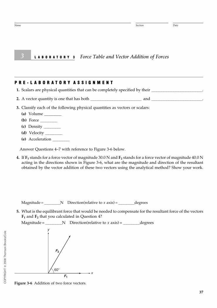
Name . . . . . . . . . . . . . . . . . . . . . . . . . . . . . . . . . . . . . . . . . . . . . . . . . . . . . . . . . . . . . . . . . . . . . . . . . Section . . . . . . . . . . . . . . . . Date . . . . . . . . . . . . . . . .
3 L A B O R A T O R Y 3 Force Table and Vector Addition of Forces
P R E - L A B O R A T O R Y A S S I G N M E N T1. Scalars are physical quantities that can be completely specified by their ______________________________.
2. A vector quantity is one that has both ______________________________ and ______________________________.
3. Classify each of the following physical quantities as vectors or scalars:
(a) Volume __________
(b) Force __________
(c) Density __________
(d) Velocity __________
(e) Acceleration __________
Answer Questions 4–7 with reference to Figure 3-6 below.
4. If F1 stands for a force vector of magnitude 30.0 N and F2 stands for a force vector of magnitude 40.0 Nacting in the directions shown in Figure 3-6, what are the magnitude and direction of the resultantobtained by the vector addition of these two vectors using the analytical method? Show your work.
Magnitude = __________N Direction(relative to x axis) = __________degrees
5. What is the equilibrant force that would be needed to compensate for the resultant force of the vectorsF1 and F2 that you calculated in Question 4?
Magnitude= __________N Direction(relative to x axis) = __________degrees
COPYRIG
HTª
2008ThomsonBrooks/Cole
y
x60°
F1
F2
Figure 3-6 Addition of two force vectors.
37

6. Figure 3-6 has been constructed to scale with 1.00 cm=10.0N. Use the parallelogram graphicalmethod to construct (on Figure 3-6) the resultant vector FR for the addition of F1 and F2. Measure thelength of the resultant vector and record it below. State the force represented by this length. Measurewith a protractor the angle that the resultant makes with the x axis.
Resultant vector length= __________cm
Force represented by this length= __________N
Direction of resultant relative to x axis = __________degrees
7. Use the polygon method of vector addition to construct on the axes below a graphical solution to theproblem in Figure 3-6. Use the scale 1.00 cm=10.0N.
Resultant vector length= __________cm
Force represented by this length= __________N
Direction of resultant relative to x axis = __________degrees
y
x
38 Physics Laboratory Manual n Loyd

Name . . . . . . . . . . . . . . . . . . . . . . . . . . . . . . . . . . . . . . . . . . . . . . . . . . . . . . . . . . . . . . . . . . . . . . . . . Section . . . . . . . . . . . . . . . . Date . . . . . . . . . . . . . . . .
Lab Partners . . . . . . . . . . . . . . . . . . . . . . . . . . . . . . . . . . . . . . . . . . . . . . . . . . . . . . . . . . . . . . . . . . . . . . . . . . . . . . . . . . . . . . . . . . . . . . . . . . . . . . . . . . . . . . . . . . . .
3 L A B O R A T O R Y 3 Force Table and Vector Addition of Forces
L A B O R A T O R Y R E P O R T
COPYRIG
HTª
2008ThomsonBrooks/Cole
Data Table 1
Force Mass (kg) Force (N) Direction
F1 0.100 20.08
F2 0.200 90.08
Equilibrant FE1
Resultant FR1
Data Table 2
Force Mass (kg) Force (N) Direction
F3 0.150 30.08
F4 0.200 100.08
F5 0.100 145.08
Equilibrant FE2
Resultant FR2
Calculations Table 1
Graphical Solution
Force Mass (kg) Force (N) Direction
F1 0.100 20.08
F2 0.200 90.08
Resultant FR1
39

P A R T 1 . E R R O R C A L C U L A T I O N S
Percent Error magnitude Experimental compared to Analytical = __________%
Percent Error magnitude Graphical compared to Analytical = __________%
Absolute Error in angle Experimental compared to Analytical = __________degrees
Absolute Error in angle Graphical compared to Analytical = __________degrees
Analytical Solution
Force Mass (kg) Force (N) Direction x-component y-component
F1 0.100 20.08
F2 0.200 90.08
Resultant FR1
Calculations Table 2
Graphical Solution
Force Mass (kg) Force (N) Direction
F3 0.150 30.08
F4 0.200 100.08
F5 0.100 145.08
Resultant FR2
Analytical Solution
Force Mass (kg) Force (N) Direction x-component y-component
F3 0.150 30.08
F4 0.200 100.08
F5 0.100 145.08
Resultant FR2
40 Physics Laboratory Manual n Loyd

P A R T 2 . E R R O R C A L C U L A T I O N S
Percent Error magnitude Experimental compared to Analytical = __________%
Percent Error magnitude Graphical compared to Analytical = __________%
Absolute Error in angle Experimental compared to Analytical = __________degrees
Absolute Error in angle Graphical compared to Analytical = __________degrees
S A M P L E C A L C U L A T I O N S1. F=mg =
2. m ¼ F
g¼
3. Direction FE opposite FR so direction FR=direction FE –1808 =
4. F1x =F1 cos (208) =
5. F1y =F1 sin (208) =
6. FR1 ¼ffiffiffiffiffiffiffiffiffiffiffiffiffiffiffiffiffiffiffiffiffiffiffiffiffiffiffiffiffiffiffiðFRxÞ2 þ ðFRyÞ2
q¼
7. y ¼ tan� 1FyFx
� ¼
8. %Error Exp ¼ jExperimental�AnalyticaljAnalytical
� 100% ¼9. Absolute Err = y (exp) – y (analytical) =
Q U E S T I O N S1. To determine the force acting on each mass it was assumed that g= 9.80m/sec2. The value of g at the
place where the experiment is performed may be slightly different from that value. State what effect(if any) it would have on the percentage error calculated for the comparisons. To test your answer to thequestion, leave g as a symbol in the calculation of the percentage error.
2. Two forces are applied to the ring of a force table, one at an angle of 20.08, and the other at an angle of80.08. Regardless of the magnitudes of the forces, choose the correct response below.
The equilibrant will be in the (a) first quadrant (b) second quadrant (c) third quadrant (d) fourthquadrant (e) cannot tell which quadrant from the available information.
COPYRIG
HTª
2008ThomsonBrooks/Cole
Laboratory 3 n Force Table and Vector Addition of Forces 41

The resultant will be in the (a) first quadrant (b) second quadrant (c) third quadrant (d) fourthquadrant (e) cannot tell which quadrant from the available information.
3. Two forces, one of magnitude 2 N and the other of magnitude 3 N, are applied to the ring of a forcetable. The directions of both forces are unknown. Which best describes the limitations on R, theresultant? Explain carefully the basis for your answer.
(a) R# 5 N (b) 2 N#R# 3 N (c) R$ 3 N (d) 1 N#R# 5 N (e) R# 2 N.
4. Suppose the same masses are used for a force table experiment as were used in Part 1, but each pulleyis moved 1808 so that the 0.100 kg mass acts at 2008, and the 0.200 kg mass acts at 2708. What is themagnitude of the resultant in this case? How does it compare to the resultant in Part 1?
5. Pulleys introduce a possible source of error because of their possible friction. Given that they are asource of error, why are the pulleys used at all? What is the function of the pulleys?
42 Physics Laboratory Manual n Loyd

Uniformly AcceleratedMotion
O B J E C T I V E So Investigate how the displacement of a cart down the inclined plane of an air track is related to
the elapsed time.
o Determine the acceleration of the cart from an analysis of the displacement versus time data.
o Determine an experimental value for g (the acceleration due to gravity) by interpretation of thecart’s acceleration as a component of g. Compare with the accepted value of g.
E Q U I P M E N T L I S T. A 5-meter linear air track with a built-in 5-meter scale (If a shorter air track is used the suggesteddistances can be modified to fit the air track used.)
. Laboratory timer or stopwatch
. Block to raise the air track to form an inclined plane
T H E O R YWhen an object undergoes one-dimensional uniformly accelerated motion its velocity increases linearlywith time. If it is assumed that the initial velocity of the object is zero at time t= 0, then its velocity v at anylater time t is given by
v ¼ at ðEq: 1Þ
where a is the acceleration, which is constant in magnitude and direction.Consider a time interval between t= 0 and any later time t. The average velocity v during the time
interval is
v ¼ 0þ v
2¼ v
2ðEq: 2Þ
The displacement x of the object during the time interval t is given by
x ¼ vt ¼ vt
2ðEq: 3Þ
Physics Laboratory Manual n Loyd L A B O R A T O R Y 4
COPYRIG
HTª
2008ThomsonBrooks/Cole
43
ª 2008 Thomson Brooks/Cole, a part of TheThomson Corporation.Thomson, the Star logo, and Brooks/Cole are trademarks used herein under license. ALL RIGHTSRESERVED.No part of this workcovered by the copyright hereonmay be reproduced or used in any form or by any meansçgraphic, electronic, ormechanical, including photocopying, recording, taping,web distribution, informationstorage and retrieval systems,or in any othermannerçwithout the written permission of the publisher.
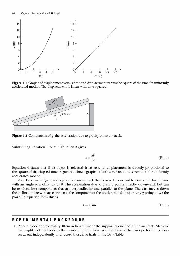
Substituting Equation 1 for v in Equation 3 gives
x ¼ at2
2ðEq: 4Þ
Equation 4 states that if an object is released from rest, its displacement is directly proportional tothe square of the elapsed time. Figure 4-1 shows graphs of both x versus t and x versus t2 for uniformlyaccelerated motion.
A cart shown in Figure 4-2 is placed on an air track that is raised at one end to form an inclined planewith an angle of inclination of y. The acceleration due to gravity points directly downward, but canbe resolved into components that are perpendicular and parallel to the plane. The cart moves downthe inclined plane with acceleration a, the component of the acceleration due to gravity g acting down theplane. In equation form this is:
a ¼ g sin y ðEq: 5Þ
E X P E R I M E N T A L P R O C E D U R E1. Place a block approximately 10 cm in height under the support at one end of the air track. Measure
the height h of the block to the nearest 0.1mm. Have five members of the class perform this mea-surement independently and record those five trials in the Data Table.
00 1 2 3 4 5 0 1 5 15 20 25
2
4
6
8
10
12
14
0
2
4
6
8
10
12
14
x (m
)
t (s) t2 (s2)
x (m
)
Figure 4-1 Graphs of displacement versus time and displacement versus the square of the time for uniformlyaccelerated motion. The displacement is linear with time squared.
g cos �
g sin �
�
gd
h
Figure 4-2 Components of g, the acceleration due to gravity on an air track.
44 Physics Laboratory Manual n Loyd
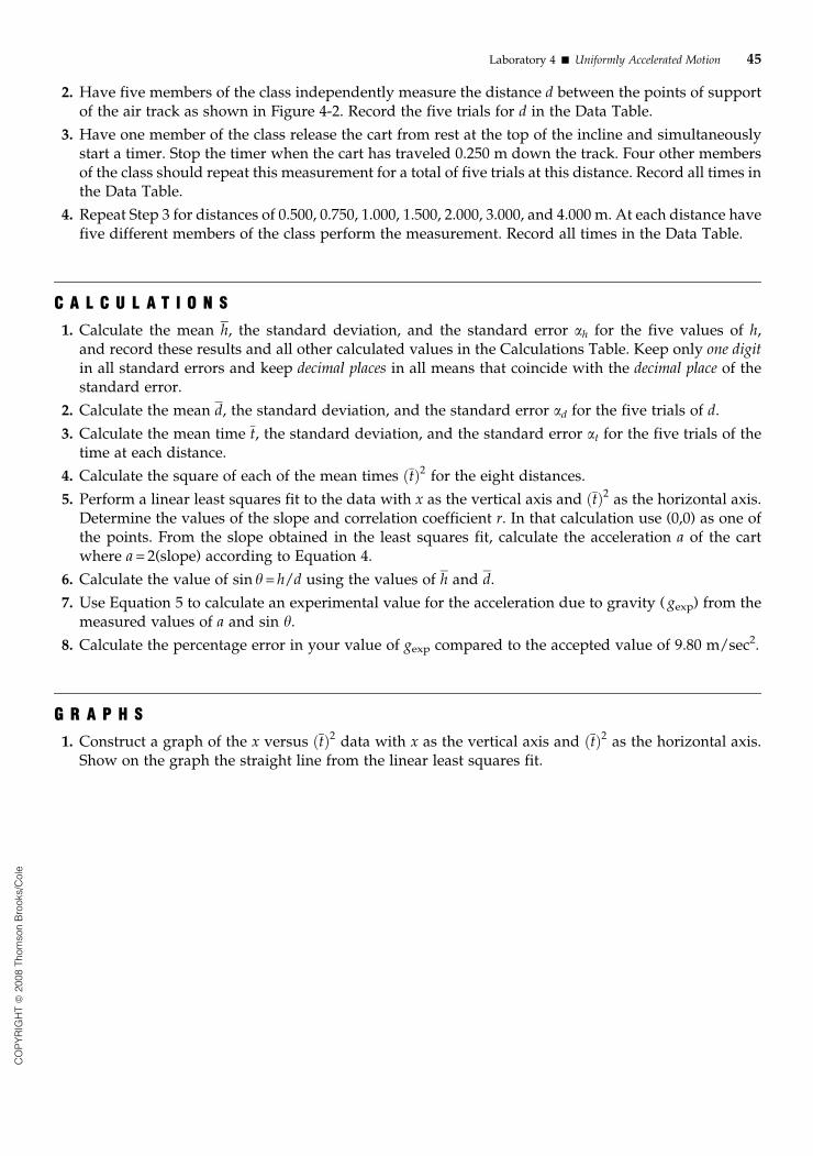
2. Have five members of the class independently measure the distance d between the points of supportof the air track as shown in Figure 4-2. Record the five trials for d in the Data Table.
3. Have one member of the class release the cart from rest at the top of the incline and simultaneouslystart a timer. Stop the timer when the cart has traveled 0.250 m down the track. Four other membersof the class should repeat this measurement for a total of five trials at this distance. Record all times inthe Data Table.
4. Repeat Step 3 for distances of 0.500, 0.750, 1.000, 1.500, 2.000, 3.000, and 4.000 m. At each distance havefive different members of the class perform the measurement. Record all times in the Data Table.
C A L C U L A T I O N S1. Calculate the mean h, the standard deviation, and the standard error ah for the five values of h,
and record these results and all other calculated values in the Calculations Table. Keep only one digitin all standard errors and keep decimal places in all means that coincide with the decimal place of thestandard error.
2. Calculate the mean d, the standard deviation, and the standard error ad for the five trials of d.
3. Calculate the mean time t, the standard deviation, and the standard error at for the five trials of thetime at each distance.
4. Calculate the square of each of the mean times ðtÞ2 for the eight distances.
5. Perform a linear least squares fit to the data with x as the vertical axis and ðtÞ2 as the horizontal axis.Determine the values of the slope and correlation coefficient r. In that calculation use (0,0) as one ofthe points. From the slope obtained in the least squares fit, calculate the acceleration a of the cartwhere a= 2(slope) according to Equation 4.
6. Calculate the value of sin y= h/d using the values of h and d.
7. Use Equation 5 to calculate an experimental value for the acceleration due to gravity ( gexp) from themeasured values of a and sin y.
8. Calculate the percentage error in your value of gexp compared to the accepted value of 9.80 m/sec2.
G R A P H S1. Construct a graph of the x versus ðtÞ2 data with x as the vertical axis and ðtÞ2 as the horizontal axis.
Show on the graph the straight line from the linear least squares fit.
COPYRIG
HTª
2008ThomsonBrooks/Cole
Laboratory 4 n Uniformly Accelerated Motion 45

This page intentionally left blank

Name . . . . . . . . . . . . . . . . . . . . . . . . . . . . . . . . . . . . . . . . . . . . . . . . . . . . . . . . . . . . . . . . . . . . . . . . . Section . . . . . . . . . . . . . . . . Date . . . . . . . . . . . . . . . .
4 L A B O R A T O R Y 4 Uniformly Accelerated Motion
P R E - L A B O R A T O R Y A S S I G N M E N T
(a)
(b)
(c)
(d)
The carts pictured above are all moving in a straight line to the right. The pictures were taken 1.00 s apart.Choose which of the descriptions below matches which pictures.
1. These pictures show a cart that is moving at constant velocity.
(a) (b) (c) (d)
2. These pictures show a cart that has a positive acceleration.
(a) (b) (c) (d)
3. These pictures show a cart that travels at a constant velocity and then has a positive acceleration.
(a) (b) (c) (d)
4. These pictures show a cart that has a negative acceleration.
(a) (b) (c) (d)
5. A cart on a linear air track has a uniform acceleration of 0.172 m/s2. Use Equation 1 to find the velocityof the cart 4.00 seconds after it is released from rest. Show your work.
COPYRIG
HTª
2008ThomsonBrooks/Cole
47
6. How far does the cart in Question 5 travel in 4.00 seconds? Calculate the distance x two ways, firstusing Equation 3 and then using Equation 4. Show your work.
7. An air track like the one shown in Figure 4-2 has a block with a height h= 12.0 cm under one support.The other support is 3.50m away. What is the angle of inclination y? According to Equation 5,the component of acceleration parallel to the track is a= g sin y where g= 9.80m/s2. For this value ofy what is a? Show your work.
48 Physics Laboratory Manual n Loyd

Name . . . . . . . . . . . . . . . . . . . . . . . . . . . . . . . . . . . . . . . . . . . . . . . . . . . . . . . . . . . . . . . . . . . . . . . . . Section . . . . . . . . . . . . . . . . Date . . . . . . . . . . . . . . . .
Lab Partners . . . . . . . . . . . . . . . . . . . . . . . . . . . . . . . . . . . . . . . . . . . . . . . . . . . . . . . . . . . . . . . . . . . . . . . . . . . . . . . . . . . . . . . . . . . . . . . . . . . . . . . . . . . . . . . . . . . .
4 L A B O R A T O R Y 4 Uniformly Accelerated Motion
L A B O R A T O R Y R E P O R T
COPYRIG
HTª
2008ThomsonBrooks/Cole
Data Table
Trial 1 Trial 2 Trial 3 Trial 4 Trial 5
h (m)
d (m)
x (m) t1 (s) t2 (s) t3 (s) t4 (s) t5 (s)
Calculations Tables
h ¼ m sn–1 = m ah= m
d ¼ m sn–1 = m ad= m
sin y ¼ h=d ¼
49
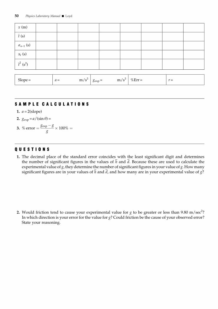
S A M P L E C A L C U L A T I O N S1. a= 2(slope)
2. gexp = a/(sin y) =
3. %error ¼ gexp� g
g� 100% ¼
Q U E S T I O N S1. The decimal place of the standard error coincides with the least significant digit and determines
the number of significant figures in the values of h and d. Because these are used to calculate theexperimental value of g, they determine the number of significant figures in your value of g. Howmanysignificant figures are in your values of h and d, and how many are in your experimental value of g?
2. Would friction tend to cause your experimental value for g to be greater or less than 9.80 m/sec2?In which direction is your error for the value for g? Could friction be the cause of your observed error?State your reasoning.
x (m)
t (s)
sn–1 (s)
at (s)
t2(s2)
Slope = a= m/s2 gexp = m/s2 %Err = r=
50 Physics Laboratory Manual n Loyd

3. What was the instantaneous velocity of the cart at x= 4.00 meters assuming your value of theacceleration a is correct? Show your work.
4. State how well the objectives of this laboratory were met. State your evidence for your opinion.
COPYRIG
HTª
2008ThomsonBrooks/Cole
Laboratory 4 n Uniformly Accelerated Motion 51

This page intentionally left blank
Uniformly AcceleratedMotion on the Air Table
O B J E C T I V E So Determine the average velocity of a puck on an inclined air table from measured displacements
and time intervals.
o Demonstrate the linear increase in the instantaneous velocity with time for the special case ofconstant acceleration, and determine the acceleration by a least squares fit to the velocity versustime data.
o Determine an experimental value for g (the acceleration due to gravity) by interpretation of thepuck’s acceleration as a component of g.
E Q U I P M E N T L I S T. Air table with sparktimer, air pump, foot switch, block, and level
. Recording paper and carbon paper
. Meter stick or measuring tape
. Balance and calibrated masses
T H E O R YTo investigate the one-dimensional motion of a puck on an air table, we choose an arbitrary point near thebeginning of the motion as the origin of the coordinate system. We determine the location of the puck bythe position x of sparks on the recording paper at a constant time interval between the marks on the paper.If the initial coordinate is xi at some time ti, and its later coordinate is xf at some later time tf, then thedisplacement Dx between those coordinates is given by
Dx ¼ xf � xi ðEq: 1Þ
Although displacements are generally vector quantities, for the special case of one-dimensional motion inone direction, it is sufficient to consider only the magnitude of the displacements. All displacements forthis laboratory will be positive because the puck moves in one direction.
Physics Laboratory Manual n Loyd L A B O R A T O R Y 5
COPYRIG
HTª
2008ThomsonBrooks/Cole
53
ª 2008 Thomson Brooks/Cole, a part of TheThomson Corporation.Thomson, the Star logo, and Brooks/Cole are trademarks used herein under license. ALL RIGHTSRESERVED.No part of this workcovered by the copyright hereonmay be reproduced or used in any form or by any meansçgraphic, electronic, ormechanical, including photocopying, recording, taping,web distribution, informationstorage and retrieval systems,or in any othermannerçwithout the written permission of the publisher.
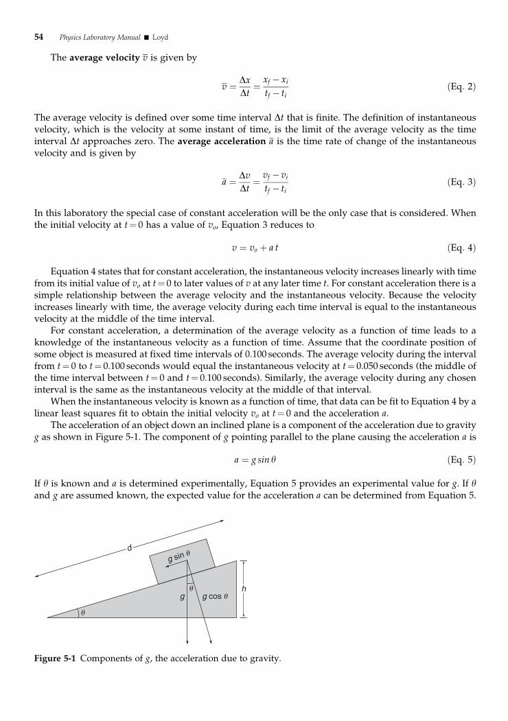
The average velocity v is given by
v ¼ DxDt
¼ xf � xitf � ti
ðEq: 2Þ
The average velocity is defined over some time interval Dt that is finite. The definition of instantaneousvelocity, which is the velocity at some instant of time, is the limit of the average velocity as the timeinterval Dt approaches zero. The average acceleration a is the time rate of change of the instantaneousvelocity and is given by
a ¼ DvDt
¼ vf � vitf � ti
ðEq: 3Þ
In this laboratory the special case of constant acceleration will be the only case that is considered. Whenthe initial velocity at t¼ 0 has a value of vo, Equation 3 reduces to
v ¼ vo þ a t ðEq: 4Þ
Equation 4 states that for constant acceleration, the instantaneous velocity increases linearly with timefrom its initial value of vo at t¼ 0 to later values of v at any later time t. For constant acceleration there is asimple relationship between the average velocity and the instantaneous velocity. Because the velocityincreases linearly with time, the average velocity during each time interval is equal to the instantaneousvelocity at the middle of the time interval.
For constant acceleration, a determination of the average velocity as a function of time leads to aknowledge of the instantaneous velocity as a function of time. Assume that the coordinate position ofsome object is measured at fixed time intervals of 0.100 seconds. The average velocity during the intervalfrom t¼ 0 to t¼ 0.100 seconds would equal the instantaneous velocity at t¼ 0.050 seconds (the middle ofthe time interval between t¼ 0 and t¼ 0.100 seconds). Similarly, the average velocity during any choseninterval is the same as the instantaneous velocity at the middle of that interval.
When the instantaneous velocity is known as a function of time, that data can be fit to Equation 4 by alinear least squares fit to obtain the initial velocity vo at t¼ 0 and the acceleration a.
The acceleration of an object down an inclined plane is a component of the acceleration due to gravityg as shown in Figure 5-1. The component of g pointing parallel to the plane causing the acceleration a is
a ¼ g sin y ðEq: 5Þ
If y is known and a is determined experimentally, Equation 5 provides an experimental value for g. If yand g are assumed known, the expected value for the acceleration a can be determined from Equation 5.
g sin �d
g cos ��
g
�
h
Figure 5-1 Components of g, the acceleration due to gravity.
54 Physics Laboratory Manual n Loyd

E X P E R I M E N T A L P R O C E D U R E1. Read the instruction manual for the air table (Figure 5-2) or obtain instructions from your laboratory
instructor. Become familiar with the operation of the air pump, the sparktimer, and the foot switch.Do not touch the conducting portions of the puck when the sparktimer is in operation.
2. Level the air table by means of the three adjustable legs until a puck placed near the center of the tableis essentially motionless.
3. Place a small block under the air table single leg to make the table act as an inclined plane. The angle ofthe inclined plane is determined by the distance between the air table legs d and the height h of theblock placed under one leg. Choose h to produce an angle of about 58. Measure h and d to the nearest0.0001meters and record them in the Data Table.
4. Set the sparktimer to a spark rate of 10.0Hertz. This will produce a spark every 0.100 seconds, and Dtbetween data points will be 0.100 seconds for all the data. Record this value of Dt in the Data Table.The values of time for x and for the center of the time interval have been included in the Data Table.
5. Place a piece of carbon paper and a sheet of recording paper on the air table with the recording paperon top. Place the two pucks on the table. To complete the circuit, both pucks must be attached to thesparktimer, but one puck can be left at rest at the bottom of the inclined plane. Simultaneously startthe sparktimer and release the other puck from rest at the top of the inclined plane. Allow the puckto accelerate down the incline while the sparktimer is in operation, but stop the sparktimer as thepuck hits the bottom rail. Release the puckwith no initial velocity. Do not impart any sidewaysmotionto the puck when releasing it.
6. Once a good spark record has been obtained, choose a point near the beginning of the track as the ori-gin and label it as x¼ 0. Call the corresponding time t¼ 0. Measure to the nearest 0.0001meters thedisplacement from the origin to each data point. Record in the Data Table the values of the coordinate xfor 12 data points. For each data point, the coordinate x is to be measured from the origin to that point.
7. Determine the mass of the puck and record it in the Data Table in kilograms.
C A L C U L A T I O N S1. Calculate the magnitude of the displacement Dx for each successive set of sparks by taking the
differences between the coordinate values for successive data points. Record the values in theCalculations Table.
2. Use Equation 2 to calculate the average velocity during each time interval from the values of Dx andthe value of Dt¼ 0.100 s. The average velocity for each interval is equal to the instantaneous velocity atC
OPYRIG
HTª
2008ThomsonBrooks/Cole
Laboratory 5 n Uniformly Accelerated Motion on the Air Table 55
Image not available due to copyright restrictions
the middle of that interval. Record the instantaneous velocity at the time each velocity occurs in theCalculations Table.
3. Perform a linear least squares fit with v as the vertical axis and t as the horizontal axis. The slopeobtained by that fit is equal to the acceleration a and the intercept obtained is equal to the initialvelocity vo. Record the acceleration, initial velocity, and correlation coefficient r in the CalculationsTable.
4. Calculate the angle of the incline y from the measured values of h and d using the equation sin y¼ h/d.Record the value of y in the Calculations Table.
5. Use the value of the acceleration a determined by the least squares fit and the measured value of yto solve Equation 5 for g. Record this experimental value of g as gexp in the Calculations Table.Calculate the percentage error for gexp compared to the true value of g¼ 9.80m/s2 and record it inthe Calculations Table.
G R A P H S1. Make a graph of the data for instantaneous velocity versus time with velocity as the vertical axis and
time as the horizontal axis. Show the data as points. Draw on the graph the straight line that wasobtained by the least squares fit procedure.
56 Physics Laboratory Manual n Loyd
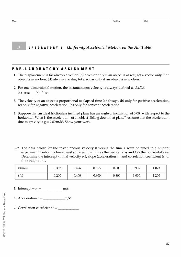
COPYRIG
HTª
2008ThomsonBrooks/Cole
Name . . . . . . . . . . . . . . . . . . . . . . . . . . . . . . . . . . . . . . . . . . . . . . . . . . . . . . . . . . . . . . . . . . . . . . . . . Section . . . . . . . . . . . . . . . . Date . . . . . . . . . . . . . . . .
5 L A B O R A T O R Y 5 Uniformly Accelerated Motion on the Air Table
P R E - L A B O R A T O R Y A S S I G N M E N T1. The displacement is (a) always a vector, (b) a vector only if an object is at rest, (c) a vector only if an
object is in motion, (d) always a scalar, (e) a scalar only if an object is in motion.
2. For one-dimensional motion, the instantaneous velocity is always defined as Dx/Dt.
(a) true (b) false
3. The velocity of an object is proportional to elapsed time (a) always, (b) only for positive acceleration,(c) only for negative acceleration, (d) only for constant acceleration.
4. Suppose that an ideal frictionless inclined plane has an angle of inclination of 5.008with respect to thehorizontal. What is the acceleration of an object sliding down that plane? Assume that the accelerationdue to gravity is g¼ 9.80m/s2. Show your work.
5–7. The data below for the instantaneous velocity v versus the time t were obtained in a studentexperiment. Perform a linear least squares fit with v as the vertical axis and t as the horizontal axis.Determine the intercept (initial velocity vo), slope (acceleration a), and correlation coefficient (r) ofthe straight line.
v (m/s) 0.352 0.496 0.655 0.808 0.939 1.073
t (s) 0.200 0.400 0.600 0.800 1.000 1.200
5. Intercept¼ vo¼ _______________m/s
6. Acceleration a¼ _______________m/s2
7. Correlation coefficient r¼ _______________
57
8. There are six data points in the Question 7 least squares fit calculation. Statistical theory states that forsix data points there is a 0.1% probability that a value of correlation coefficient r$ 0.974 will beobtained for uncorrelated data. Compare the value of r obtained in Question 7 to 0.974. State yourconclusion about the probability that these data show that velocity is proportional to time.
9. Assume that the data of Question 5–7 were taken for an inclined plane of angle 4.408. Equation 5 statesthat the acceleration down the plane is a¼ g sin y. Use this equation to determine an experimentalvalue for g from the acceleration a determined in Question 6. Calculate the percentage error betweenthis experimental value gexp and the true value of 9.80m/s2.
gexp¼ _______________m/s2 Percentage error¼ _______________%
58 Physics Laboratory Manual n Loyd
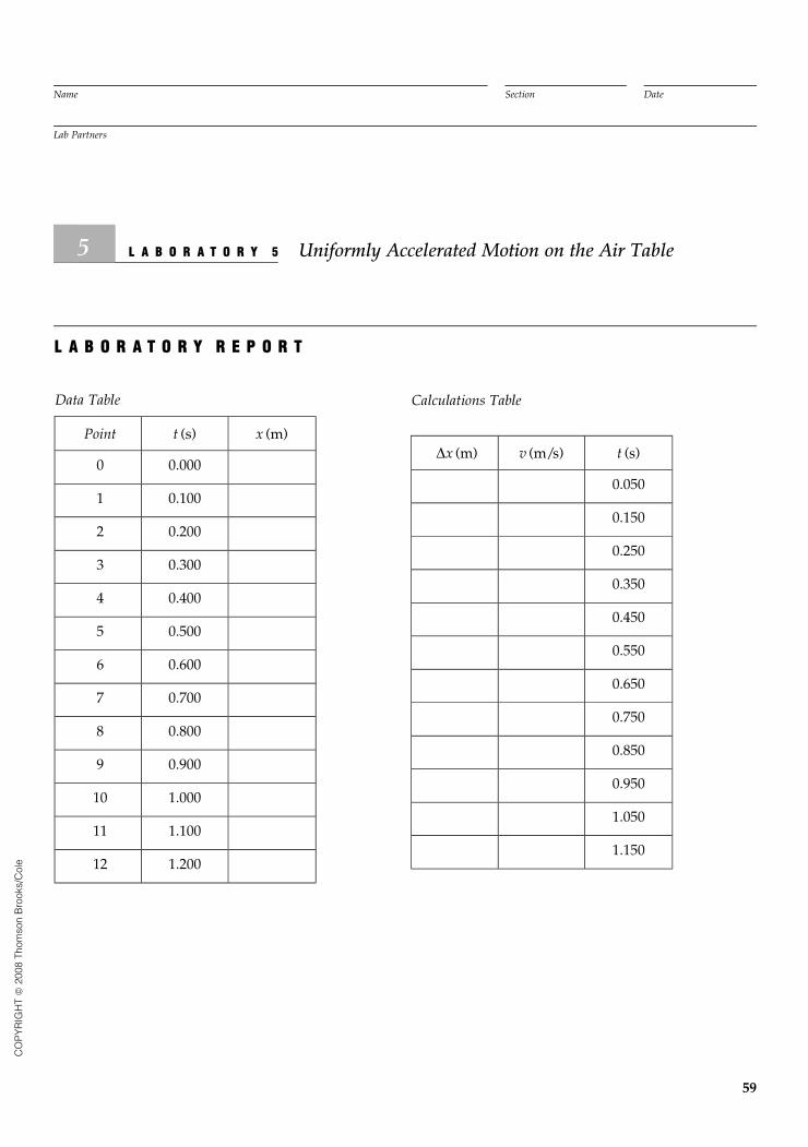
Name . . . . . . . . . . . . . . . . . . . . . . . . . . . . . . . . . . . . . . . . . . . . . . . . . . . . . . . . . . . . . . . . . . . . . . . . . Section . . . . . . . . . . . . . . . . Date . . . . . . . . . . . . . . . .
Lab Partners . . . . . . . . . . . . . . . . . . . . . . . . . . . . . . . . . . . . . . . . . . . . . . . . . . . . . . . . . . . . . . . . . . . . . . . . . . . . . . . . . . . . . . . . . . . . . . . . . . . . . . . . . . . . . . . . . . . .
5 L A B O R A T O R Y 5 Uniformly Accelerated Motion on the Air Table
L A B O R A T O R Y R E P O R T
COPYRIG
HTª
2008ThomsonBrooks/Cole
Data Table
Point t (s) x (m)
0 0.000
1 0.100
2 0.200
3 0.300
4 0.400
5 0.500
6 0.600
7 0.700
8 0.800
9 0.900
10 1.000
11 1.100
12 1.200
Calculations Table
Dx (m) v (m/s) t (s)
0.050
0.150
0.250
0.350
0.450
0.550
0.650
0.750
0.850
0.950
1.050
1.150
59
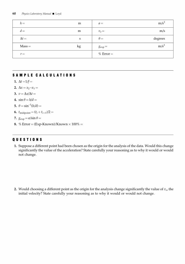
h¼ m a¼ m/s2
d¼ m vo¼ m/s
Dt¼ s y¼ degrees
Mass¼ kg gexp¼ m/s2
r¼ % Error¼
S A M P L E C A L C U L A T I O N S1. Dt¼1/f¼2. Dx¼ x2 –x1¼3. v¼Dx/Dt¼4. sin y¼ h/d¼5. y¼ sin–1(h/d)¼6. tmidpoint¼ (tiþ tiþ1)/2¼7. gexp¼ a/sin y¼8. %Error¼ (Exp-Known)/Known� 100%¼
Q U E S T I O N S1. Suppose a different point had been chosen as the origin for the analysis of the data. Would this change
significantly the value of the acceleration? State carefully your reasoning as to why it would or wouldnot change.
2. Would choosing a different point as the origin for the analysis change significantly the value of vo, theinitial velocity? State carefully your reasoning as to why it would or would not change.
60 Physics Laboratory Manual n Loyd

3. How long before the time you chose as zero for your analysis was the puck actually released?(Hint—Consider the time at which v¼ 0 in Equation 4.)
4. There are 12 data points in the linear least squares fit to Equation 4. Statistical theory states that there isonly a 0.1% probability (1 chance in 1000) of achieving a value of r$ 0.823 for 12 data points ofuncorrelated data. State the most complete assessment you can make about how well your dataconfirm the theory.
COPYRIG
HTª
2008ThomsonBrooks/Cole
Laboratory 5 n Uniformly Accelerated Motion on the Air Table 61

This page intentionally left blank

Kinematics in TwoDimensions on the Air Table
O B J E C T I V E So Investigate the trajectory of a puck on a tilted air table.
o Determine the acceleration ay in the y direction by taking the slope of a graph of the y componentof velocity vy versus time.
o Determine the very slight negative acceleration in the x direction due to friction from the veryslight negative slope of vx versus time.
E Q U I P M E N T L I S T. Air table with sparktimer, air pump, foot switch, level, and carbon paper
. Recording paper, ruler, square, and protractor
T H E O R YIn Figure 6-1 an object is launched at an angle y relative to the horizontal (x axis) and moves in a two-dimensional path. If vo is the magnitude of its velocity, then its initial velocity in the x direction isvo cos y, and its initial velocity in the y direction is vo sin y. Assuming no friction, there is no accelerationin the x direction, and the x component of velocity is constant in time. There is an acceleration in thenegative y direction, opposite in direction to the initial y component of velocity. The two equations thatdescribe the x and y components of velocity vx and vy as a function of time are
vx ¼ vo cos y ðEq: 1Þ
vy ¼ vo sin y� ay t ðEq: 2Þ
In Equation 2 the direction of the acceleration has been shown by the negative sign, and ay stands for themagnitude of the acceleration.
Assume that values of the x and y coordinates are known for some general two-dimensional motion.If xi and xf stand for the x coordinate positions at the initial time ti and final time tf, and yi and yf stand forthe y coordinate positions at these same times, then the displacements Dx and Dy during the time intervalDt are given by
Physics Laboratory Manual n Loyd L A B O R A T O R Y 6
COPYRIG
HTª
2008ThomsonBrooks/Cole
63
ª 2008 Thomson Brooks/Cole, a part of TheThomson Corporation.Thomson, the Star logo, and Brooks/Cole are trademarks used herein under license. ALL RIGHTSRESERVED.No part of this workcovered by the copyright hereonmay be reproduced or used in any form or by any meansçgraphic, electronic, ormechanical, including photocopying, recording, taping,web distribution, informationstorage and retrieval systems,or in any othermannerçwithout the written permission of the publisher.
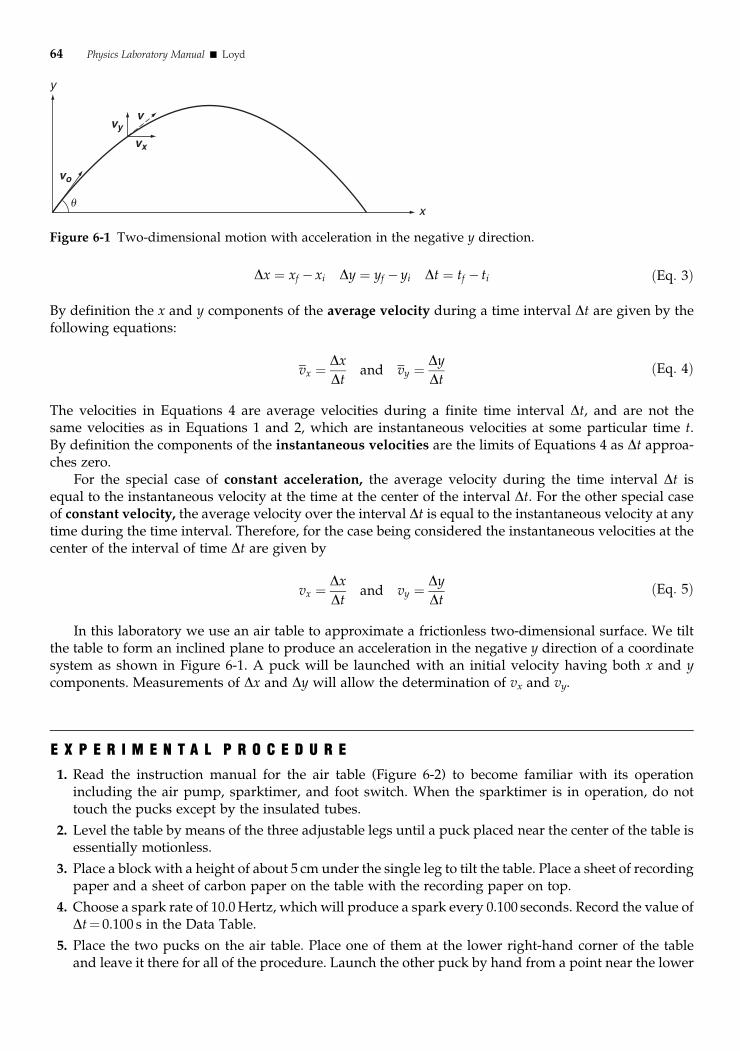
Dx ¼ xf � xi Dy ¼ yf � yi Dt ¼ tf � ti ðEq: 3Þ
By definition the x and y components of the average velocity during a time interval Dt are given by thefollowing equations:
vx ¼ DxDt
and vy ¼ DyDt
ðEq: 4Þ
The velocities in Equations 4 are average velocities during a finite time interval Dt, and are not thesame velocities as in Equations 1 and 2, which are instantaneous velocities at some particular time t.By definition the components of the instantaneous velocities are the limits of Equations 4 as Dt approa-ches zero.
For the special case of constant acceleration, the average velocity during the time interval Dt isequal to the instantaneous velocity at the time at the center of the interval Dt. For the other special caseof constant velocity, the average velocity over the interval Dt is equal to the instantaneous velocity at anytime during the time interval. Therefore, for the case being considered the instantaneous velocities at thecenter of the interval of time Dt are given by
vx ¼ DxDt
and vy ¼ DyDt
ðEq: 5Þ
In this laboratory we use an air table to approximate a frictionless two-dimensional surface. We tiltthe table to form an inclined plane to produce an acceleration in the negative y direction of a coordinatesystem as shown in Figure 6-1. A puck will be launched with an initial velocity having both x and ycomponents. Measurements of Dx and Dy will allow the determination of vx and vy.
E X P E R I M E N T A L P R O C E D U R E1. Read the instruction manual for the air table (Figure 6-2) to become familiar with its operation
including the air pump, sparktimer, and foot switch. When the sparktimer is in operation, do nottouch the pucks except by the insulated tubes.
2. Level the table by means of the three adjustable legs until a puck placed near the center of the table isessentially motionless.
3. Place a block with a height of about 5 cm under the single leg to tilt the table. Place a sheet of recordingpaper and a sheet of carbon paper on the table with the recording paper on top.
4. Choose a spark rate of 10.0Hertz, which will produce a spark every 0.100 seconds. Record the value ofDt¼ 0.100 s in the Data Table.
5. Place the two pucks on the air table. Place one of them at the lower right-hand corner of the tableand leave it there for all of the procedure. Launch the other puck by hand from a point near the lower
vy
vx
vo
y
x�
v
Figure 6-1 Two-dimensional motion with acceleration in the negative y direction.
64 Physics Laboratory Manual n Loyd
left-hand corner of the table. The puck should move upward and to the right and approach near thetop center of the tilted table, and then move down to the vicinity of the lower right-hand corner.Several practice launches will probably be necessary to determine the correct launch speed anddirection needed to achieve the desired trajectory.
6. When, after enough practice, you are sure that you can achieve the desired path, launch the puck andstart the sparktimer simultaneously. Stop the sparktimer just before the puck arrives at the lowerright-hand corner. Be sure that there are about 20 or so good data points on the record. Do not removethe sheet of recording paper after making this measurement! Instead, record a second trace on this same paper toexperimentally determine the vertical (y direction). This vertical trace is obtained by releasing the puckfrom a point near the top of the table on the same side of the air table fromwhich the puck is launched.
7. Remove the recording sheet for data analysis. Choose as the origin the lowest point on the trajectorythat comes out clearly and call the corresponding time zero. Label that first point as 0 and then labelthe next 15 consecutive data points. Note that the times corresponding to these points are alreadygiven in the Data Table.
8. Draw a straight line through the vertical line formed by the sparktimer trace for the puck fallingvertically. This defines the vertical direction.
9. Construct a straight line that passes through the origin chosen above in Step 7 and parallel to thevertical line drawn in Step 8. This is the y axis of the coordinate system. Construct a line through theorigin and perpendicular to the y axis. This is the x axis of the coordinate system.
10. Measure the perpendicular distance of each data point from the y axis. Record these values in the DataTable as the values of the coordinate x.
11. Measure the perpendicular distance of each data point from the x axis. Record these values in the DataTable as the values of the coordinate y.
C A L C U L A T I O N S1. Calculate the differences between the successive values of x and y and record them in the Calculations
Table as the values of Dx and Dy. Note that Dy will change in magnitude, and it will become negativeafter the puck reaches its maximum height and starts back down.
2. Use Equations 5 to calculate the components of the instantaneous velocity vx and vy and record themin the Calculations Table. The time at which the instantaneous velocities apply are at the center ofeach interval, and those times have already been recorded in the Calculations Table for each interval.
3. Perform a linear least squares fit with vx as the vertical axis and t as the horizontal axis. The slope ofthis fit should be very small and negative, and it is equal to the acceleration caused by friction.C
OPYRIG
HTª
2008ThomsonBrooks/Cole
Laboratory 6 n Kinematics in Two Dimensions on the Air Table 65
Image not available due to copyright restrictions

The intercept is the initial velocity in the x direction (vx)o. Record the values of ax, (vx)o, and r in theCalculations Table.
4. Perform a linear least squares fit with vy as the vertical axis and time as the horizontal axis. The slopeof this fit is equal to the acceleration in the y direction, and the intercept is the initial velocity in they direction (vy)o. Record the values of ay, (vy)o, and r in the Calculations Table.
G R A P H S1. On one sheet of graph paper, graph both vx and vy as a function of time. Use different symbols for vx
and vy. Because vy can have both positive and negative values, choose the origin of the velocity scale inthe center of the graph paper. Include the straight lines obtained by the least squares fit for each case.
66 Physics Laboratory Manual n Loyd

Name . . . . . . . . . . . . . . . . . . . . . . . . . . . . . . . . . . . . . . . . . . . . . . . . . . . . . . . . . . . . . . . . . . . . . . . . . Section . . . . . . . . . . . . . . . . Date . . . . . . . . . . . . . . . .
6 L A B O R A T O R Y 6 Kinematics in Two Dimensions on the Air Table
P R E - L A B O R A T O R Y A S S I G N M E N T
Assume that the projectile motion shown in Figure 6-1 is ideal with no friction. For that assumption,choose the correct statements about the motion in 1 and 2 below.
1. (a) The value of vx is always positive and decreases very slightly with time. (b) The value of vx changesfrom positive to negative with time. (c) The value of vx is always negative and increases very slightlywith time. (d) The value of vx is always positive and is constant with time. (e) The value of vx changesfrom negative to positive with time.
2. (a) The value of vy is always positive and decreases very slightly with time. (b) The value of vy changesfrom positive to negative with time. (c) The value of vy is always negative and increases very slightlywith time. (d) The value of vy is always positive and is constant with time. (e) The value of vy changesfrom negative to positive with time.
Assume now for the projectile motion shown in Figure 6-1 that there is a very small frictional forceacting on the puck. For that assumption, choose the correct statements about the motion in 3 and 4below.
3. (a) The value of vx is always positive and decreases very slightly with time. (b) The value of vx changesfrom positive to negative with time. (c) The value of vx is always negative and increases very slightlywith time. (d) The value of vx is always positive and is constant with time. (e) The value of vx changesfrom negative to positive with time.
4. (a) The value of ax is zero. (b) The value of ax is very small and negative. (c) The value of ax is verysmall and positive. (d) The value of ax changes from positive to negative. (e) The value of ax changesfrom negative to positive.
A particle moves in such a way that its coordinate positions x and y as a function of time aregiven by the following table.
x(m) 0.000 0.550 1.100 1.650 2.200 2.750 3.300 3.850 4.400
y(m) 0.000 1.425 2.700 3.825 4.800 5.625 6.300 6.825 7.200
t(s) 0.000 0.100 0.200 0.300 0.400 0.500 0.600 0.700 0.800
Answer the following questions (5 through 7) with respect to these data.
COPYRIG
HTª
2008ThomsonBrooks/Cole
67

5. What is the particle’s average velocity in the y direction vy between t¼ 0.200 s and t¼ 0.300 s? Whatis vy between t¼ 0.400 s and t¼ 0.500 s?What is vy between t¼ 0.700 s and t¼ 0.800 s? Show yourwork.
6. What is the particle’s average velocity in the x direction vx between t¼ 0.200 s and t¼ 0.300 s? What isvx between t¼ 0.400 s and t¼ 0.500 s? What is vx between t¼ 0.700 s and t¼ 0.800 s? Show your work.
7. What is the particle’s instantaneous velocity in the y direction vy at t¼ 0.250 s? What is vy at t¼ 0.450 s?What is vy at t¼ 0.750 s? (Hint—Assume that the average velocity during a time interval is equal to theinstantaneous velocity at the center of the time interval.) Show your work.
68 Physics Laboratory Manual n Loyd

Name . . . . . . . . . . . . . . . . . . . . . . . . . . . . . . . . . . . . . . . . . . . . . . . . . . . . . . . . . . . . . . . . . . . . . . . . . Section . . . . . . . . . . . . . . . . Date . . . . . . . . . . . . . . . .
Lab Partners . . . . . . . . . . . . . . . . . . . . . . . . . . . . . . . . . . . . . . . . . . . . . . . . . . . . . . . . . . . . . . . . . . . . . . . . . . . . . . . . . . . . . . . . . . . . . . . . . . . . . . . . . . . . . . . . . . . .
6 L A B O R A T O R Y 6 Kinematics in Two Dimensions on the Air Table
L A B O R A T O R Y R E P O R T
COPYRIG
HTª
2008ThomsonBrooks/Cole
Data Table
t(s) x(m) y(m)
0.000
0.100
0.200
0.300
0.400
0.500
0.600
0.700
0.800
0.900
1.000
1.100
1.200
1.300
1.400
1.500
Calculations Table
Dx(m) Dy(m) vx(m/s) vy(m/s) t(s)
0.050
0.150
0.250
0.350
0.450
0.550
0.650
0.750
0.850
0.950
1.050
1.150
1.250
1.350
1.450
69
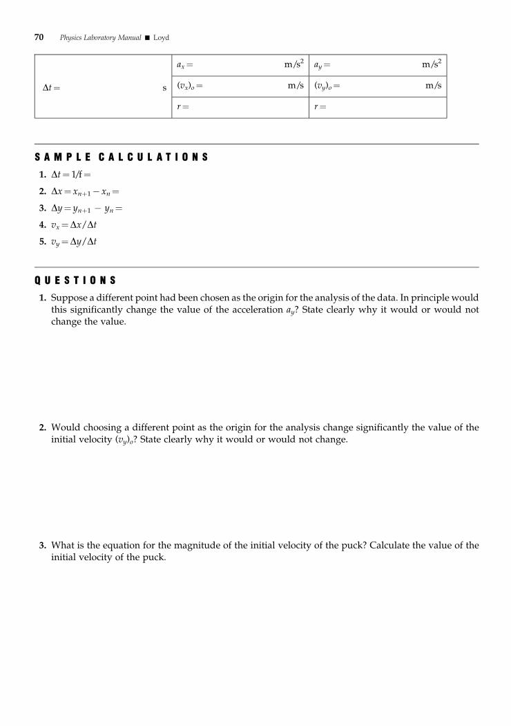
S A M P L E C A L C U L A T I O N S1. Dt¼ 1/f¼2. Dx¼ xnþ1� xn¼3. Dy¼ ynþ1 � yn¼4. vx¼Dx/Dt
5. vy¼Dy/Dt
Q U E S T I O N S1. Suppose a different point had been chosen as the origin for the analysis of the data. In principle would
this significantly change the value of the acceleration ay? State clearly why it would or would notchange the value.
2. Would choosing a different point as the origin for the analysis change significantly the value of theinitial velocity (vy)o? State clearly why it would or would not change.
3. What is the equation for the magnitude of the initial velocity of the puck? Calculate the value of theinitial velocity of the puck.
Dt¼ s
ax¼ m/s2 ay¼ m/s2
(vx)o¼ m/s (vy)o¼ m/s
r¼ r¼
70 Physics Laboratory Manual n Loyd

4. Calculate the ratio of the magnitude of ax to the magnitude of ay.
5. The small negative value of ax is due to friction. If the ratio calculated in Question 4 is 0.02, it wouldindicate that friction is about a 2% effect. If the ratio were 0.01 it would indicate that friction isapproximately a 1% effect. Based on your value of that ratio, estimate how large an effect friction wasin your data.
COPYRIG
HTª
2008ThomsonBrooks/Cole
Laboratory 6 n Kinematics in Two Dimensions on the Air Table 71

This page intentionally left blank
Coefficient of Friction
O B J E C T I V E So Determine ms, the static coefficient of friction, and mk, the kinetic coefficient of friction, by sliding
the block down a board that acts as an inclined plane.
o Determine ms and mk using the board with a pulley mounted on it in a horizontal position andapplying known forces to the block.
o Compare the different values for ms and mk obtained by the two different techniques.
o Demonstrate that the coefficients are independent of the normal force, and that ms>mk.
E Q U I P M E N T L I S T. Smooth wooden board with pulley attached to one end
. Smooth wooden block (6-inch long 2�4 for example) with hook attached
. Second wooden block of known length to form inclined plane
. String, balance, calibrated masses, mass holder, and slotted masses
T H E O R YFriction is a resisting force that acts along the tangent to two surfaces in contact when one body slides orattempts to slide across another.Normal force is the force that each body exerts on the other body, and itacts perpendicular to each surface. The frictional force is directly proportional to the normal force.
There are two different kinds of friction. Static friction occurs when two surfaces are still at rest withrespect to each other, but an attempt is being made to cause one of them to slide over the other one. Staticfriction arises to oppose any force trying to cause motion tangent to the surfaces. The static frictional forcefs is given by
fs #msN ðEq: 1Þ
whereN stands for the normal force between the two surfaces, and ms is a constant called the coefficient ofstatic friction. The meaning of Equation 1 is that the static frictional force varies in response to appliedforces from zero up to a maximum value given by the equality in that equation. If the applied force is lessthan themaximum, then the frictional force that arises is equal to the applied force, and there is nomotion.If the applied force is greater than the maximum, the object will begin to move, and static frictionconditions are no longer valid.
Physics Laboratory Manual n Loyd L A B O R A T O R Y 7
COPYRIG
HTª
2008ThomsonBrooks/Cole
73
ª 2008 Thomson Brooks/Cole, a part of TheThomson Corporation.Thomson, the Star logo, and Brooks/Cole are trademarks used herein under license. ALL RIGHTSRESERVED.No part of this workcovered by the copyright hereonmay be reproduced or used in any form or by any meansçgraphic, electronic, ormechanical, including photocopying, recording, taping,web distribution, informationstorage and retrieval systems,or in any othermannerçwithout the written permission of the publisher.

The other kind of friction occurs when two surfaces are moving with respect to each other. It is calledkinetic friction, and it is characterized by a constant mk called the coefficient of kinetic friction. Thekinetic frictional force fk is given by
fk ¼ mk N ðEq: 2Þ
where N is again the normal force. Equation 2 states that the kinetic frictional force is a constant valueany time the object is in motion. In fact, the coefficient of kinetic friction does vary somewhat withspeed. It is assumed for this laboratory that at the slow speeds used, mk does not depend upon speed. To agood approximation both coefficients are independent of the apparent area of contact between the twosurfaces.
An inclined plane with an angle y that can be adjusted is shown in Figure 7-1. If a block is placed onthe plane, and the angle is slowly increased, the block will begin to slip at some angle. The normal forceN acts perpendicularly to the plane, and a component of the weight of the block mg cos ys acts in theopposite direction. The block is in equilibrium for motion perpendicular to the plane, and these forcesare equal and
N ¼ mg cos ys ðEq: 3Þ
where ys is the angle at which the block just begins to slip on the inclined plane. Parallel to the plane thereare also two forces. A component of the weight of the block mg sin ys acts down the plane, and thefrictional force fs acts up the plane. At the point where the block just slips, the maximum frictional force isexerted, and these two forces are equal. In equation form
fs ¼ msN ¼ mg sin ys ðEq: 4Þ
Combining Equations 3 and 4 leads to
ms ¼mg sin ys
N¼ mg sin ys
mg cos y2¼ tan ys ðEq: 5Þ
Equation 5 can be used to determine ms by measuring tan ys when the block just begins to slip on theinclined plane.
In a similar way the same inclined plane can be used to determine mk. By giving the block a slight pushto get it started, the angle can be determined at which the block slides down the plane at constant velocity.A push is needed to get it started because generally ms>mk, and the static frictional force is greater than the
mg cos �
mg sin �
N
mg
f
�
�
Figure 7-1 Forces acting on a block on an inclined plane.
74 Physics Laboratory Manual n Loyd

kinetic frictional force. When the block is moving down the plane at constant velocity, the block is inequilibrium with the vector sum of forces on the block equal to zero. In equation form
N ¼ mg cos yk and fk ¼ mg sin yk ¼ mkN ðEq: 6Þ
Using algebra to combine these equations leads to
mk ¼mg sin yk
N¼ mg sin yk
mg cos yk¼ tan yk ðEq: 7Þ
Equation 7 can be used to determine mk from the angle at which the block slides down the inclined plane atconstant velocity after it has been given a slight push to get it started.
If the inclined board is lowered to the horizontal position, a force can be applied to the block bymeansof a string running over a pulley and down to a mass as shown in Figure 7-2. For a given block massM1 itis possible to slowly add mass to M2 until M1 moves. The point at which the block just moves is the lastpoint that the system is in equilibrium, and it occurs when the maximum static friction is acting. At thatpoint the following conditions are met:
T ¼ fs T ¼ M2g N ¼ M1g fs ¼ msN ðEq: 8Þ
In these equations T is the tension in the string, and the other symbols are the same as previously defined.Combining these four equations leads to
fs ¼ M2g ¼ ms N ¼ msM1g ðEq: 9Þ
Using the second and fourth terms above and canceling the common factor of g gives
M2 ¼ msM1 ðEq: 10Þ
Equation 10 can be used to determine ms by finding the minimum mass M2 needed to cause the block ofmass M1 to just move.
The same procedure can also be used to determine the coefficient of kinetic friction. Refer to Figure 7-2and imagine that fs is replaced by fk for the case when the block is in motion.When the system is moving atconstant velocity it is also in equilibrium, and the following conditions are met:
T ¼ fk T ¼ M2g N ¼ M1g fk ¼ mkN ðEq: 11Þ
COPYRIG
HTª
2008ThomsonBrooks/Cole
fs T
T
N
M1g
M2g
M1
M2
Figure 7-2 Force applied to a block on a horizontal plane.
Laboratory 7 n Coefficient of Friction 75
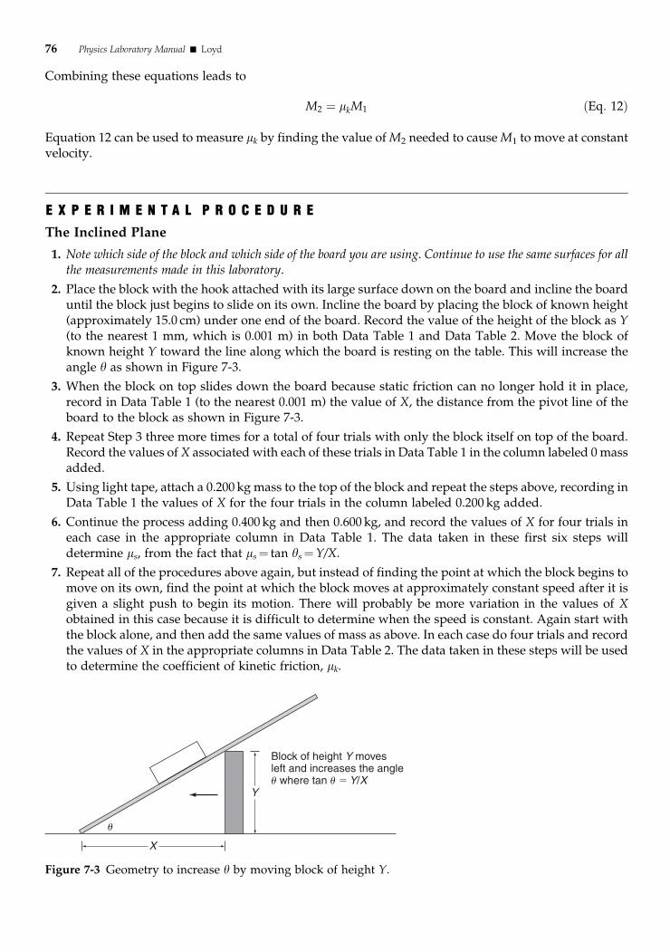
Combining these equations leads to
M2 ¼ mkM1 ðEq: 12Þ
Equation 12 can be used to measure mk by finding the value ofM2 needed to causeM1 to move at constantvelocity.
E X P E R I M E N T A L P R O C E D U R EThe Inclined Plane
1. Note which side of the block and which side of the board you are using. Continue to use the same surfaces for allthe measurements made in this laboratory.
2. Place the block with the hook attached with its large surface down on the board and incline the boarduntil the block just begins to slide on its own. Incline the board by placing the block of known height(approximately 15.0 cm) under one end of the board. Record the value of the height of the block as Y(to the nearest 1 mm, which is 0.001 m) in both Data Table 1 and Data Table 2. Move the block ofknown height Y toward the line along which the board is resting on the table. This will increase theangle y as shown in Figure 7-3.
3. When the block on top slides down the board because static friction can no longer hold it in place,record in Data Table 1 (to the nearest 0.001 m) the value of X, the distance from the pivot line of theboard to the block as shown in Figure 7-3.
4. Repeat Step 3 three more times for a total of four trials with only the block itself on top of the board.Record the values ofX associated with each of these trials in Data Table 1 in the column labeled 0 massadded.
5. Using light tape, attach a 0.200 kg mass to the top of the block and repeat the steps above, recording inData Table 1 the values of X for the four trials in the column labeled 0.200 kg added.
6. Continue the process adding 0.400 kg and then 0.600 kg, and record the values of X for four trials ineach case in the appropriate column in Data Table 1. The data taken in these first six steps willdetermine ms, from the fact that ms¼ tan ys¼Y/X.
7. Repeat all of the procedures above again, but instead of finding the point at which the block begins tomove on its own, find the point at which the block moves at approximately constant speed after it isgiven a slight push to begin its motion. There will probably be more variation in the values of Xobtained in this case because it is difficult to determine when the speed is constant. Again start withthe block alone, and then add the same values of mass as above. In each case do four trials and recordthe values of X in the appropriate columns in Data Table 2. The data taken in these steps will be usedto determine the coefficient of kinetic friction, mk.
Block of height Y movesleft and increases the angle� where tan � � Y/X
Y
X
�
Figure 7-3 Geometry to increase y by moving block of height Y.
76 Physics Laboratory Manual n Loyd
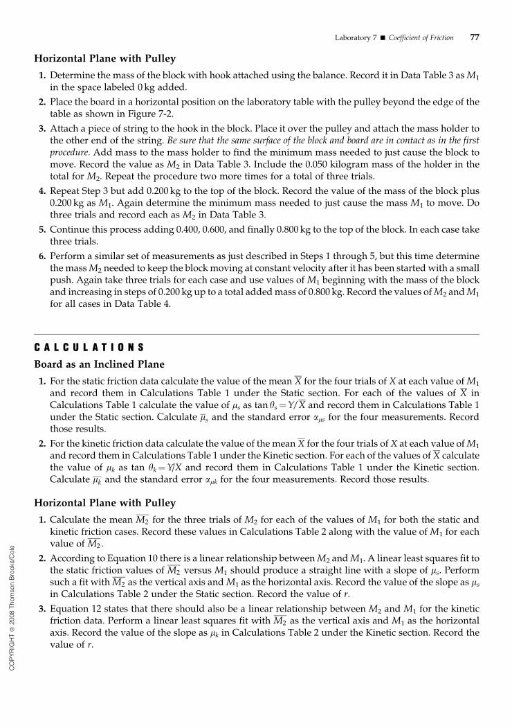
Horizontal Plane with Pulley
1. Determine the mass of the block with hook attached using the balance. Record it in Data Table 3 asM1
in the space labeled 0 kg added.
2. Place the board in a horizontal position on the laboratory table with the pulley beyond the edge of thetable as shown in Figure 7-2.
3. Attach a piece of string to the hook in the block. Place it over the pulley and attach the mass holder tothe other end of the string. Be sure that the same surface of the block and board are in contact as in the firstprocedure. Add mass to the mass holder to find the minimum mass needed to just cause the block tomove. Record the value as M2 in Data Table 3. Include the 0.050 kilogram mass of the holder in thetotal for M2. Repeat the procedure two more times for a total of three trials.
4. Repeat Step 3 but add 0.200 kg to the top of the block. Record the value of the mass of the block plus0.200 kg as M1. Again determine the minimum mass needed to just cause the mass M1 to move. Dothree trials and record each as M2 in Data Table 3.
5. Continue this process adding 0.400, 0.600, and finally 0.800 kg to the top of the block. In each case takethree trials.
6. Perform a similar set of measurements as just described in Steps 1 through 5, but this time determinethe massM2 needed to keep the block moving at constant velocity after it has been started with a smallpush. Again take three trials for each case and use values of M1 beginning with the mass of the blockand increasing in steps of 0.200 kg up to a total addedmass of 0.800 kg. Record the values ofM2 andM1
for all cases in Data Table 4.
C A L C U L A T I O N SBoard as an Inclined Plane
1. For the static friction data calculate the value of the mean X for the four trials of X at each value ofM1
and record them in Calculations Table 1 under the Static section. For each of the values of X inCalculations Table 1 calculate the value of ms as tan ys¼Y/X and record them in Calculations Table 1under the Static section. Calculate ms and the standard error ams for the four measurements. Recordthose results.
2. For the kinetic friction data calculate the value of the meanX for the four trials ofX at each value ofM1
and record them in Calculations Table 1 under the Kinetic section. For each of the values ofX calculatethe value of mk as tan yk¼Y/X and record them in Calculations Table 1 under the Kinetic section.Calculate mk and the standard error amk for the four measurements. Record those results.
Horizontal Plane with Pulley
1. Calculate the mean M2 for the three trials of M2 for each of the values of M1 for both the static andkinetic friction cases. Record these values in Calculations Table 2 along with the value of M1 for eachvalue of M2 .
2. According to Equation 10 there is a linear relationship betweenM2 andM1. A linear least squares fit tothe static friction values of M2 versus M1 should produce a straight line with a slope of ms. Performsuch a fit withM2 as the vertical axis andM1 as the horizontal axis. Record the value of the slope as msin Calculations Table 2 under the Static section. Record the value of r.
3. Equation 12 states that there should also be a linear relationship between M2 and M1 for the kineticfriction data. Perform a linear least squares fit with M2 as the vertical axis and M1 as the horizontalaxis. Record the value of the slope as mk in Calculations Table 2 under the Kinetic section. Record thevalue of r.
COPYRIG
HTª
2008ThomsonBrooks/Cole
Laboratory 7 n Coefficient of Friction 77

G R A P H S1. Graph the static friction data for the horizontal plane case with M2 as the vertical axis and M1 as the
horizontal axis. Show the straight line obtained from the fit.
2. Graph the kinetic friction data for the horizontal plane case withM2 as the vertical axis andM1 as thehorizontal axis. Show the straight line obtained from the fit.
78 Physics Laboratory Manual n Loyd
Name . . . . . . . . . . . . . . . . . . . . . . . . . . . . . . . . . . . . . . . . . . . . . . . . . . . . . . . . . . . . . . . . . . . . . . . . . Section . . . . . . . . . . . . . . . . Date . . . . . . . . . . . . . . . .
7 L A B O R A T O R Y 7 Coefficient of Friction
P R E - L A B O R A T O R Y A S S I G N M E N T1. For kinetic friction the direction of the frictional force on a given object is always opposite the direction
of that object’s motion. (a) true (b) false
2. The two coefficients of friction discussed in this laboratory are static (ms) and kinetic (mk). Describe theconditions under which each kind is appropriate. Generally, which of the two is larger?
3. Suppose a block of mass 25.0 kg rests on a horizontal plane, and the coefficient of static frictionbetween the surfaces is 0.220. (a) What is the maximum possible static frictional force that could act onthe block? _______________N (b) What is the actual static frictional force that acts on the block if anexternal force of 25.0 N acts horizontally on the block? _______________N Assume g¼ 9.80m/s2. Showyour work and explain both answers.
4. To measure the coefficient of kinetic friction by sliding a block down an inclined plane the block mustbe in equilibrium. What experimental condition must you try to accomplish that will assure you thatthe block is in equilibrium?
COPYRIG
HTª
2008ThomsonBrooks/Cole
79

5. A 5.00 kg block rests on a horizontal plane. A force of 10.0 N applied horizontally causes the block tomove horizontally at constant velocity. What is the coefficient of kinetic friction between the block andthe plane? Assume g¼ 9.80m/sec2. Show your work.
6. Both types of coefficient of friction are dimensionless. Why is this true?
7. For either type of coefficient of friction, what is generally assumed about the dependence of the valueof the coefficient on the area of contact between the two surfaces?
80 Physics Laboratory Manual n Loyd

Name . . . . . . . . . . . . . . . . . . . . . . . . . . . . . . . . . . . . . . . . . . . . . . . . . . . . . . . . . . . . . . . . . . . . . . . . . Section . . . . . . . . . . . . . . . . Date . . . . . . . . . . . . . . . .
Lab Partners . . . . . . . . . . . . . . . . . . . . . . . . . . . . . . . . . . . . . . . . . . . . . . . . . . . . . . . . . . . . . . . . . . . . . . . . . . . . . . . . . . . . . . . . . . . . . . . . . . . . . . . . . . . . . . . . . . . .
7 L A B O R A T O R Y 7 Coefficient of Friction
L A B O R A T O R Y R E P O R T
Data Table 1 Inclined Plane—Static Friction
Y¼ _______________m
Added Mass 0.000 kg 0.200 kg 0.400 kg 0.600 kg
M1 (kg)
X Trial 1 (m)
X Trial 2 (m)
X Trial 3 (m)
X Trial 4 (m)
Data Table 2 Inclined Plane—Kinetic Friction
Y¼ _______________m
Added Mass 0.000 kg 0.200 kg 0.400 kg 0.600 kg
M1 (kg)
X Trial 1 (m)
X Trial 2 (m)
X Trial 3 (m)
X Trial 4 (m)
COPYRIG
HTª
2008ThomsonBrooks/Cole
81

Data Table 3 Horizontal Plane—Static Friction
Added Mass 0.000 kg 0.200 kg 0.400 kg 0.600 kg 0.800 kg
M1 (kg)
M2 Trial 1
M2 Trial 2
M2 Trial 3
Data Table 4 Horizontal Plane—Kinetic Friction
Added Mass 0.000 kg 0.200 kg 0.400 kg 0.600 kg 0.800 kg
M1 (kg)
M2 Trial 1
M2 Trial 2
M2 Trial 3
Calculations Table 1—Inclined Plane
Static
X (m) ms¼Y/X ms ams
Kinetic
X (m) mk ¼Y/X mk amk
Calculations Table 2—Horizontal Plane
Static
M1 (kg) M2 (kg) ms r
Kinetic
M1 (kg) M2 (kg) mk r
82 Physics Laboratory Manual n Loyd
S A M P L E C A L C U L A T I O N S1. X¼ (X1þX2þX3þX4)/4¼2. ms¼Y/X¼3. Percent Difference for m¼
Q U E S T I O N S1. Discuss the agreement between the two different measured values of ms. Calculate the percentage
difference between them. Percentage difference¼_______________%. Assume that the error in thehorizontal plane value is approximately equal to the standard error for the inclined plane data. Underthe assumption that both values of ms have that same error, do the two values of ms overlap within thatassumed error? State the range of each measurement and quantitatively state the extent to which theyoverlap.
2. Answer the same questions as asked in Question 1, but now consider the kinetic friction data.Percentage difference¼ _______________%.
3. To what extent do your data confirm the expectation that the coefficients of friction, both static andkinetic, are independent of the normal force?What is the evidence for the inclined plane data?What isthe evidence for the horizontal plane data? Give as quantitative an answer as possible in both cases.
4. Do your data confirm the expectation that ms$ mk? Comment for both values of each coefficient andstate your evidence.
COPYRIG
HTª
2008ThomsonBrooks/Cole
Laboratory 7 n Coefficient of Friction 83

5. State clearly in your own words what was to be accomplished in this laboratory. To what extent didyour performance of the laboratory accomplish those goals?
84 Physics Laboratory Manual n Loyd

Newton’s Second Lawon the Air Table
O B J E C T I V E So Investigate the variation in the acceleration produced when different forces are applied to a fixed
mass.
o Demonstrate that the acceleration is proportional to the applied force.
o Determine the frictional force that acts on the system.
E Q U I P M E N T L I S T. Air table with pucks, sparktimer, air pump, foot switch, and level
. Carbon paper, recording paper, meter stick or tape
. Pulley, string, laboratory balance, and calibrated masses
T H E O R YThe relationship between the net force F exerted on a body of mass m and the acceleration a of the body isNewton’s Second Law.
F ¼ ma ðEq: 1Þ
A mass m1 is shown in Figure 8-1 on a horizontal surface. It is connected to a second mass m2 by a stringrunning over a pulley. There is tension T in the string connecting the masses. Each mass is subject toseveral forces shown in a free body diagram in Figure 8-2. Four forces act on mass m1, but only two ofthem lie along the direction of motion of the mass. The weight of m1 and the normal force from the tableare equal in magnitude and opposite in direction and sum to zero. The net force acting on m1 is equal toT� f and Equation 1 gives
T � f ¼ m1a ðEq: 2Þ
The two forces acting on mass m2 are its weight m2g and the tension T. Because m1 and m2 are connected,the acceleration of m2 has the same magnitude as the acceleration of m1. In equation form
m2g� T ¼ m2a ðEq: 3Þ
Physics Laboratory Manual n Loyd L A B O R A T O R Y 8
COPYRIG
HTª
2008ThomsonBrooks/Cole
85
ª 2008 Thomson Brooks/Cole, a part of TheThomson Corporation.Thomson, the Star logo, and Brooks/Cole are trademarks used herein under license. ALL RIGHTSRESERVED.No part of this workcovered by the copyright hereonmay be reproduced or used in any form or by any meansçgraphic, electronic, ormechanical, including photocopying, recording, taping,web distribution, informationstorage and retrieval systems,or in any othermannerçwithout the written permission of the publisher.

If Equations 2 and 3 are combined and f added to both sides, the result is
m2g ¼ ðm1 þm2Þaþ f ðEq: 4Þ
Equation 4 assumes that f represents all the friction in the system including the pulley.We will make a series of measurements varying the applied forcem2gwhile the mass (m1þm2) is kept
constant. We will measure the resulting acceleration a of the masses as a function of the force m2g. Thecoordinate position x of the puck as a function of time t will be measured using a sparktimer to mark x attime intervals of 0.100 seconds. The average velocity v during any time interval Dt is
v ¼ DxDt
ðEq: 5Þ
where Dx is the displacement during the time interval Dt. Because the acceleration is constant, the averagevelocity v during time intervalDt is the instantaneous velocity v at the time t at the center ofDt. The equation
v ¼ DxDt
ðEq: 6Þ
gives the instantaneous velocity v at the center of time interval Dt. From the resulting values of v as afunction of time, we will determine the acceleration a.
E X P E R I M E N T A L P R O C E D U R E1. Read the instruction manual for the air table (Figure 8-3) to become familiar with its operation,
including the air pump, sparktimer, and foot switch. Do not touch the pucks when the sparktimer is inoperation except by the insulated tubes.
N
T
T
f m2
m1g
m2g
m1
Figure 8-2 Free body diagram of the forces on masses m1 and m2.
T
T
gm1
m2
Figure 8-1 Force applied to mass m1 by weight of mass m2.
86 Physics Laboratory Manual n Loyd
2. Level the table by means of the three adjustable legs until a puck placed near the center of the table isessentially motionless. Place a sheet of carbon paper and a sheet of recording paper on the table withthe recording paper on top.
3. Place one of the pucks in the corner of the table and leave it there for the rest of the procedure. Placethe other puck on a laboratory balance and determine its massmp. Record the value ofmp in kg in Dataand Calculations Table 1.
4. Place the puck for which mass has been determined on the air table. Attach a string to the puck. Runthe string over the pulley as shown in Figure 8-1 and attach a mass of 0.010 kg on the end of the stringto serve as mass m2.
5. Place mass totaling 0.040 kg on top of the puck. The total mass m1þm2 is equal to the puck mass mp
plus the 0.040 kg plus the 0.0100 kg on the end of the string. Record this value (mpþ 0.050 kg) in Dataand Calculations Table 1 as m1þm2.
6. Choose a spark rate of 20.0 Hertz. Release the puck near the edge of the table with zero velocity andsimultaneously start the sparktimer. Stop the sparktimer just before the puck reaches the other side ofthe table. Release the puck with no initial velocity.
7. Remove 0.010 kg from the puck and add it to the 0.010 kg on the end of the string so that m2 is now0.020 kg, butm1þm2 remains the same. Slide the recording paper over slightly, again release the puckwith no initial velocity, and record this trace with the sparktimer.
8. Continue this process, each time shifting 0.010 kg from the puck to the end of the string to producetraces with values of m2 equal to 0.030, 0.040, and 0.050 kg while the value of m1þm2 remains fixed.Record all five traces on the same sheet of paper.
9. Choose an origin for each of the five traces and label every other point. This will produce data pointswith time intervals of Dt¼ 0.100 seconds. Measure the values of the coordinate position x as a functionof time from t¼ 0 to t¼ 0.600 seconds for each of the traces. Record the values of x in Data andCalculations Table 1.
C A L C U L A T I O N S1. Calculate the values of the displacement Dx between successive data points for each of the five traces.
Record the values of Dx in Data and Calculations Table 1.
2. Use Equation 6 to calculate the instantaneous velocity at the times corresponding to the center of themeasured time intervals. Record the values of v at the appropriate instantaneous times in Data andCalculations Table 1.C
OPYRIG
HTª
2008ThomsonBrooks/Cole
Laboratory 8 n Newton’s Second Law on the Air Table 87
Image not available due to copyright restrictions
3. From the values of m2 using g¼ 9.80m/s2, calculate the values m2g for each of the applied forces.Record the results in Data and Calculations Table 2.
4. Perform a linear least squares fit to each of the five sets of v versus t data with v as the vertical axis andt as the horizontal axis. Record the values of the slope for each fit as the acceleration a in Data andCalculations Table 2. Record the values of the intercept of each fit as the initial velocity in the table.Record the values of the correlation coefficient r in the table.
5. Equation 4 states that a is proportional tom2gwithm1þm2 as the constant of proportionality. Performa linear least squares fit with m2g as the vertical axis and a as the horizontal axis. Record in Data andCalculations Table 2 the slope of the fit as (m1þm2)exp the experimental value for the total mass.Record in Data and Calculations Table 2 the intercept of the fit as f the friction.
6. Calculate the percentage error in the value of (m1þm2)exp compared to the known value of m1þm2
and record it in Data and Calculations Table 2.
G R A P H S1. On a single sheet of graph paper plot the data for the v versus t for each of the five cases. Also show on
the graph the straight line obtained by each fit to the data. Use different symbols to label the fivedifferent sets of data.
2. Make a graph of the data for the applied force m2g versus the acceleration a. Also show on the graphthe straight line obtained by the fit to the data.
88 Physics Laboratory Manual n Loyd
Name . . . . . . . . . . . . . . . . . . . . . . . . . . . . . . . . . . . . . . . . . . . . . . . . . . . . . . . . . . . . . . . . . . . . . . . . . Section . . . . . . . . . . . . . . . . Date . . . . . . . . . . . . . . . .
8 L A B O R A T O R Y 8 Newton’s Second Law on the Air Table
P R E - L A B O R A T O R Y A S S I G N M E N T1. A net force of 25.0 N acts on a 6.50-kg object. What is the acceleration of the object? Show your work.
2. In Figures 8-1 and 8-2, what are the two forces acting on mass m1 that must be considered indetermining the acceleration of the mass? Why don’t the other forces have to be considered?
3. Suppose that a 0.450-kg puck (m1) is attached to a 0.0400-kg mass (m2) as shown in Figure 8-1. Aconstant frictional force f¼ 0.100N acts on the puck. Solve Equation 4 for the acceleration a. Show yourwork.
4. What is the weight (in N) of a mass of 0.050 kg? Show your work.
COPYRIG
HTª
2008ThomsonBrooks/Cole
89

The following data for coordinate position x versus time t were taken for a puck that is uniformly
accelerated.
5. Calculate the displacement Dx during each time interval and record each of them in the table above.Calculate the instantaneous velocity v at the center of each time interval and record each of them in thetable above. Show sample calculations.
6. For the data in the table above perform a linear least squares fit with v the vertical axis and t thehorizontal axis. Record the slope of this fit as the acceleration a of the puck. Record the intercept of thefit as the initial velocity vo. (This is the calculation that you will do five times in the laboratory.)
a¼ ____________________m/s2
vo¼ ____________________m/s
t (s) 0.000 0.100 0.200 0.300 0.400 0.500 0.600
x (m) 0.000 0.0102 0.0399 0.0896 0.1603 0.2498 0.3607
Dx (m)
v (m/s)
t (s) 0.050 0.150 0.250 0.350 0.450 0.550
90 Physics Laboratory Manual n Loyd

Name . . . . . . . . . . . . . . . . . . . . . . . . . . . . . . . . . . . . . . . . . . . . . . . . . . . . . . . . . . . . . . . . . . . . . . . . . Section . . . . . . . . . . . . . . . . Date . . . . . . . . . . . . . . . .
Lab Partners . . . . . . . . . . . . . . . . . . . . . . . . . . . . . . . . . . . . . . . . . . . . . . . . . . . . . . . . . . . . . . . . . . . . . . . . . . . . . . . . . . . . . . . . . . . . . . . . . . . . . . . . . . . . . . . . . . . .
8 L A B O R A T O R Y 8 Newton’s Second Law on the Air Table
L A B O R A T O R Y R E P O R T
COPYRIG
HTª
2008ThomsonBrooks/Cole
Data and Calculations Table 1
Dt¼ 0.100 s mp¼ kg m1þm2¼ kg
t (s) 0.000 0.100 0.200 0.300 0.400 0.500 0.600
x (m)
m2
.0100kg
Dx (m)
v (m/s)
t (s) 0.050 0.150 0.250 0.350 0.450 0.550
t (s) 0.000 0.100 0.200 0.300 0.400 0.500 0.600
x (m)
m2
.0200kg
Dx (m)
v (m/s)
t (s) 0.050 0.150 0.250 0.350 0.450 0.550
t (s) 0.000 0.100 0.200 0.300 0.400 0.500 0.600
x (m)
m2
.0300kg
Dx (m)
v (m/s)
t (s) 0.050 0.150 0.250 0.350 0.450 0.550
91
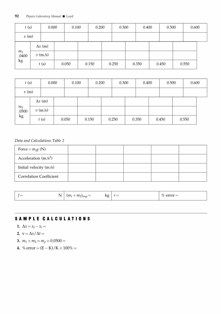
S A M P L E C A L C U L A T I O N S1. Dx¼ xf� xi¼2. v¼Dx/Dt¼3. m1þm2¼mpþ 0.0500¼4. %error¼ (E�K)/K� 100%¼
t (s) 0.000 0.100 0.200 0.300 0.400 0.500 0.600
x (m)
m2
.0400kg
Dx (m)
v (m/s)
t (s) 0.050 0.150 0.250 0.350 0.450 0.550
t (s) 0.000 0.100 0.200 0.300 0.400 0.500 0.600
x (m)
m2
.0500kg
Dx (m)
v (m/s)
t (s) 0.050 0.150 0.250 0.350 0.450 0.550
Data and Calculations Table 2
Force¼m2g (N)
Acceleration (m/s2)
Initial velocity (m/s)
Correlation Coefficient
f¼ N (m1þm2)exp¼ kg r¼ % error¼
92 Physics Laboratory Manual n Loyd

Q U E S T I O N S1. Each of your five graphs of v versus t contains six data points. According to statistical theory for six
data points there is only 0.1% probability (1 chance in 1000) that uncorrelated data would giver$ 0.974. State how your values of r compare to 0.974, and make the best statement you can about thevalidity of the correlation of these data.
2. Your graph of applied force versus acceleration contains five data points, and statistical theoryindicates that for five points there is a 1% probability that r$ 0.959 would be obtained for uncorrelateddata. From your value of r make the best statement you can about the validity of the correlation ofyour data.
3. What is the ratio of the frictional force f to the applied force m2g for each case? For which of the cases(if any) is f less than 10% of m2g? Based on this, what is your conclusion about the importance offriction in your data?
4. Summarize the concepts investigated in this laboratory. What was to be proved, and how confidentare you that your data confirm the theory?
COPYRIG
HTª
2008ThomsonBrooks/Cole
Laboratory 8 n Newton’s Second Law on the Air Table 93

This page intentionally left blank

Newton’s Second Law onAtwood’s Machine
O B J E C T I V E So Investigate the acceleration produced by a series of different forces applied to a fixed mass, and
demonstrate that the acceleration is proportional to the applied force.
o Demonstrate that the constant of proportionality between the acceleration and the applied forceis the mass to which the force is applied.
o Determine the frictional force that acts on the system.
E Q U I P M E N T L I S T. Atwood’s machine pulley (very low-friction ball-bearing pulley)
. Calibrated slotted masses, slotted mass holders, laboratory balance
. Laboratory timer (capable of measuring to 0.01 s), strong thin nylon string, and meter stick
T H E O R YThe relationship between the net force F exerted on a mass m and the acceleration a of the mass isNewton’s Second Law.
F ¼ ma ðEq: 1Þ
The system shown in Figure 9-1 is called an Atwood’s machine. It consists of twomasses at the ends ofa string passing over a pulley. Also shown in the figure is a free-body diagram of the forces. For m2 > m1,Equation 1 applied to each mass gives
T�m1g ¼ m1a and m2g�T ¼ m2a ðEq: 2Þ
where T is the tension in the string, and a is the magnitude of the acceleration of either mass. CombiningEquations 2 leads to
ðm2 �m1Þg ¼ ðm1 þm2Þa ðEq: 3Þ
Physics Laboratory Manual n Loyd L A B O R A T O R Y 9
COPYRIG
HTª
2008ThomsonBrooks/Cole
95
ª 2008 Thomson Brooks/Cole, a part of TheThomson Corporation.Thomson, the Star logo, and Brooks/Cole are trademarks used herein under license. ALL RIGHTSRESERVED.No part of this workcovered by the copyright hereonmay be reproduced or used in any form or by any meansçgraphic, electronic, ormechanical, including photocopying, recording, taping,web distribution, informationstorage and retrieval systems,or in any othermannerçwithout the written permission of the publisher.
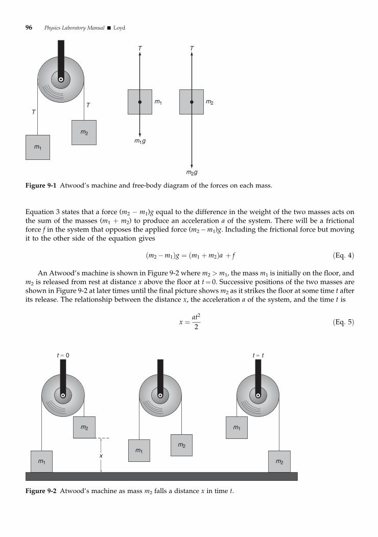
Equation 3 states that a force (m2 � m1)g equal to the difference in the weight of the two masses acts onthe sum of the masses (m1 þ m2) to produce an acceleration a of the system. There will be a frictionalforce f in the system that opposes the applied force (m2�m1)g. Including the frictional force but movingit to the other side of the equation gives
ðm2 �m1Þg ¼ ðm1 þm2Þa þ f ðEq: 4Þ
An Atwood’s machine is shown in Figure 9-2 where m2 > m1, the mass m1 is initially on the floor, andm2 is released from rest at distance x above the floor at t¼ 0. Successive positions of the two masses areshown in Figure 9-2 at later times until the final picture showsm2 as it strikes the floor at some time t afterits release. The relationship between the distance x, the acceleration a of the system, and the time t is
x ¼ at2
2ðEq: 5Þ
T
m1
m2
m1 m2
m1g
m2g
T
T T
Figure 9-1 Atwood’s machine and free-body diagram of the forces on each mass.
m1
m2
m2
x
t � 0 t � t
m1
m1
m2
m2
Figure 9-2 Atwood’s machine as mass m2 falls a distance x in time t.
96 Physics Laboratory Manual n Loyd
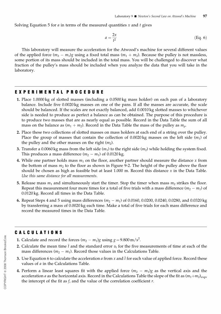
Solving Equation 5 for a in terms of the measured quantities x and t gives
a ¼ 2x
t2ðEq: 6Þ
This laboratory will measure the acceleration for the Atwood’s machine for several different valuesof the applied force (m2 � m1)g using a fixed total mass (m1 þ m2). Because the pulley is not massless,some portion of its mass should be included in the total mass. You will be challenged to discover whatfraction of the pulley’s mass should be included when you analyze the data that you will take in thelaboratory.
E X P E R I M E N T A L P R O C E D U R E1. Place 1.0000 kg of slotted masses (including a 0.0500 kg mass holder) on each pan of a laboratory
balance. Include five 0.0020 kg masses on one of the pans. If all the masses are accurate, the scaleshould be balanced. If the scales are not exactly balanced, add 0.0010 kg slotted masses to whicheverside is needed to produce as perfect a balance as can be obtained. The purpose of this procedure isto produce two masses that are as nearly equal as possible. Record in the Data Table the sum of allmass on the balance as (m1 þ m2). Record in the Data Table the mass of the pulley as mp.
2. Place these two collections of slotted masses on mass holders at each end of a string over the pulley.Place the group of masses that contain the collection of 0.0020 kg masses on the left side (m1) ofthe pulley and the other masses on the right (m2).
3. Transfer a 0.0060 kg mass from the left side (m1) to the right side (m2) while holding the system fixed.This produces a mass difference (m2 � m1) of 0.0120 kg.
4. While one partner holds mass m1 on the floor, another partner should measure the distance x fromthe bottom of mass m2 to the floor as shown in Figure 9-2. The height of the pulley above the floorshould be chosen as high as feasible but at least 1.000 m. Record this distance x in the Data Table.Use this same distance for all measurements.
5. Release mass m1 and simultaneously start the timer. Stop the timer when mass m2 strikes the floor.Repeat this measurement four more times for a total of five trials with a mass difference (m2 � m1) of0.0120 kg. Record all times in the Data Table.
6. Repeat Steps 4 and 5 using mass differences (m2 � m1) of 0.0160, 0.0200, 0.0240, 0.0280, and 0.0320 kgby transferring a mass of 0.0020 kg each time. Make a total of five trials for each mass difference andrecord the measured times in the Data Table.
C A L C U L A T I O N S1. Calculate and record the forces (m2 � m1)g using g¼ 9.800m/s2.
2. Calculate the mean time t and the standard error at for the five measurements of time at each of themass differences (m2 � m1). Record those values in the Calculations Table.
3. Use Equation 6 to calculate the acceleration a from x and t for each value of applied force. Record thesevalues of a in the Calculations Table.
4. Perform a linear least squares fit with the applied force (m2 � m1)g as the vertical axis and theacceleration a as the horizontal axis. Record in the Calculations Table the slope of the fit as (m1þm2)exp,the intercept of the fit as f, and the value of the correlation coefficient r.
COPYRIG
HTª
2008ThomsonBrooks/Cole
Laboratory 9 n Newton’s Second Law on Atwood’s Machine 97

G R A P H S1. Make a graph of the data with the applied force as the vertical axis and the acceleration as the
horizontal axis. Also show on the graph the straight line obtained by the least squares fit to the data.
98 Physics Laboratory Manual n Loyd
Name . . . . . . . . . . . . . . . . . . . . . . . . . . . . . . . . . . . . . . . . . . . . . . . . . . . . . . . . . . . . . . . . . . . . . . . . . Section . . . . . . . . . . . . . . . . Date . . . . . . . . . . . . . . . .
9 L A B O R A T O R Y 9 Newton’s Second Law on Atwood’s Machine
P R E - L A B O R A T O R Y A S S I G N M E N T1. A net force of 3.50N acts on a 2.75 kg object. What is the acceleration of the object? Show your work.
2. Describe the basic concept of the Atwood’s machine. What is the net applied force? What is the massto which this net force is applied? Show your work.
3. An Atwood’s machine consists of a 1.060 kg mass and a 1.000 kg mass connected by a string over amassless and frictionless pulley. Use Equation 3 to find the acceleration of the system. Assume that gis 9.80 m/s2. Show your work.
4. Suppose that the system in Question 3 has a frictional force of 0.056 N. Use Equation 4 to determinethe acceleration of the system. Show your work.
COPYRIG
HTª
2008ThomsonBrooks/Cole
99
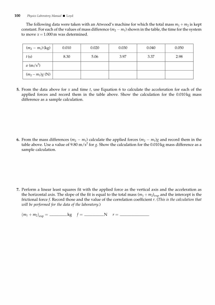
The following data were taken with an Atwood’s machine for which the total mass m1þm2 is keptconstant. For each of the values of mass difference (m2�m1) shown in the table, the time for the systemto move x¼ 1.000m was determined.
(m2 � m1) (kg) 0.010 0.020 0.030 0.040 0.050
t (s) 8.30 5.06 3.97 3.37 2.98
a (m/s2)
(m2�m1)g (N)
5. From the data above for x and time t, use Equation 6 to calculate the acceleration for each of theapplied forces and record them in the table above. Show the calculation for the 0.010 kg massdifference as a sample calculation.
6. From the mass differences (m2 � m1) calculate the applied forces (m2 � m1)g and record them in thetable above. Use a value of 9.80 m/s2 for g. Show the calculation for the 0.010 kg mass difference as asample calculation.
7. Perform a linear least squares fit with the applied force as the vertical axis and the acceleration asthe horizontal axis. The slope of the fit is equal to the total mass (m1þm2)exp and the intercept is thefrictional force f. Record those and the value of the correlation coefficient r. (This is the calculation thatwill be performed for the data of the laboratory.)
ðm1 þm2Þexp ¼ kg f ¼ N r ¼
100 Physics Laboratory Manual n Loyd

Name . . . . . . . . . . . . . . . . . . . . . . . . . . . . . . . . . . . . . . . . . . . . . . . . . . . . . . . . . . . . . . . . . . . . . . . . . Section . . . . . . . . . . . . . . . . Date . . . . . . . . . . . . . . . .
Lab Partners . . . . . . . . . . . . . . . . . . . . . . . . . . . . . . . . . . . . . . . . . . . . . . . . . . . . . . . . . . . . . . . . . . . . . . . . . . . . . . . . . . . . . . . . . . . . . . . . . . . . . . . . . . . . . . . . . . . .
9 L A B O R A T O R Y 9 Newton’s Second Law on Atwood’s Machine
L A B O R A T O R Y R E P O R T
COPYRIG
HTª
2008ThomsonBrooks/Cole
Data Table
(m1þm2)¼ kg mp¼ kg x¼ m
(m2�m1) (kg) t1 (s) t2 (s) t3 (s) t4 (s) t5 (s)
0.012
0.016
0.020
0.024
0.028
0.032
Calculations Table
(m2�m1)g (N) t (s) at (s) a (m/s2)
(m1þm2)exp¼ kg f¼ N r¼
101

S A M P L E C A L C U L A T I O N S1. % Error¼ (E�K)/K� 100%¼
Q U E S T I O N S1. According to statistical theory for six data points there is only 1% probability (1 chance in 100) that a
value of r� 0.917 and a 0.1% probability (1 chance in 1000) that a value of r� 0.974 would be obtainedfor data that are uncorrelated. Based on this idea, what does your value of r indicate for the level ofcorrelation of your data?
2. Divide the frictional force by the applied force, (m2 � m1)g, for each applied force and express it as apercentage in the space below. Friction would not be important if these percentages were a fewpercent, would be small if they were about 10%, and would be very important if they were 25% orgreater. Make the best possible statement about the importance of friction for your data.
3. Your value of (m1þm2)exp should be greater than your recorded value of (m1þm2) because of theeffect of the pulley. Perform the calculations needed to determine what fraction of the pulley’s massappears to be included in your value of (m1þm2)exp. If you were to express that fraction as a wholenumber fraction, which of the following would best fit your data? (½ �̂̄ ¼ �̂̇ )
102 Physics Laboratory Manual n Loyd

4. The laboratory instructed you to transfer mass from one side of the pulley to the other side. Why wasthis procedure used instead of just adding mass to one side of the pulley to produce a larger force?
5. What concept is this laboratory designed to investigate? Describe the extent to which your data andanalysis validate the concept.
COPYRIG
HTª
2008ThomsonBrooks/Cole
Laboratory 9 n Newton’s Second Law on Atwood’s Machine 103

This page intentionally left blank

Torques and RotationalEquilibrium of a Rigid Body
O B J E C T I V E So Apply the conditions for equilibrium of a rigid body to a meter stick pivoted on a knife edge.
o Determine the center of gravity of the meter stick, mass of the meter stick, and mass of anunknown object by applying known torques.
o For a given applied force needed to produce equilibrium, compare the theoretically predictedlocation of the force to an experimentally determined location.
E Q U I P M E N T L I S T. Meter stick with adjustable knife-edge clamp and support stand
. Laboratory balance and calibrated hooked masses
. Thin nylon thread and unknown mass with hook
T H E O R YIf a force F acts on a rigid body that is pivoted about some axis, the body tends to rotate about that axis.The tendency of a force to cause a body to rotate about some axis is measured by a quantity calledtorque t. It is defined by
t ¼ Fd\ ðEq: 1Þ
with F the magnitude of the force, and d\ the lever arm of the force. The units of torque are N–m.Torque caused by a given force must be defined relative to a specific axis of rotation. Figure 10-1 showstwo forces F1 and F2 acting on an arbitrarily shaped body.
The axis of rotation is along a line through O perpendicular to the page. The direction of the line ofaction of each force is shown as a dotted line extended in either direction along the force vector. The leverarm for each force is shown as the perpendicular distance from O to the line of action of the force. In thiscase there are two torques t1 and t2 acting on the body given by
t1 ¼ F1d1 and t2 ¼ F2d2 ðEq: 2Þ
Physics Laboratory Manual n Loyd L A B O R A T O R Y 10
COPYRIG
HTª
2008ThomsonBrooks/Cole
105
ª 2008 Thomson Brooks/Cole, a part of TheThomson Corporation.Thomson, the Star logo, and Brooks/Cole are trademarks used herein under license. ALL RIGHTSRESERVED.No part of this workcovered by the copyright hereonmay be reproduced or used in any form or by any meansçgraphic, electronic, ormechanical, including photocopying, recording, taping,web distribution, informationstorage and retrieval systems,or in any othermannerçwithout the written permission of the publisher.
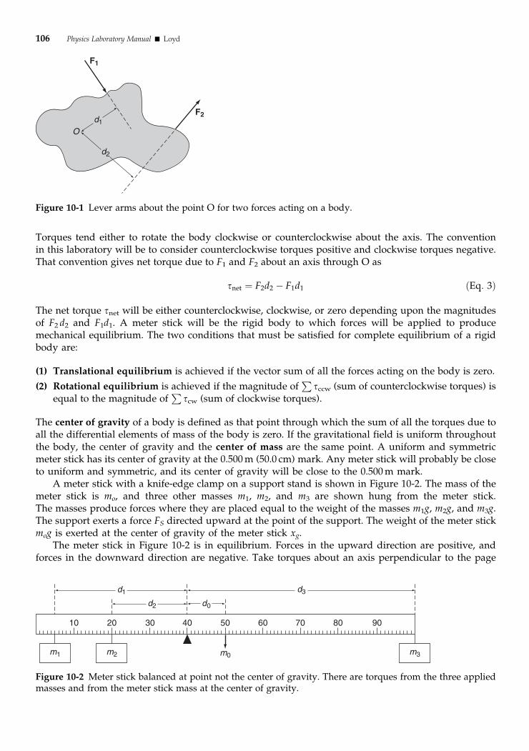
Torques tend either to rotate the body clockwise or counterclockwise about the axis. The conventionin this laboratory will be to consider counterclockwise torques positive and clockwise torques negative.That convention gives net torque due to F1 and F2 about an axis through O as
tnet ¼ F2d2 � F1d1 ðEq: 3Þ
The net torque tnet will be either counterclockwise, clockwise, or zero depending upon the magnitudesof F2 d2 and F1d1. A meter stick will be the rigid body to which forces will be applied to producemechanical equilibrium. The two conditions that must be satisfied for complete equilibrium of a rigidbody are:
(1) Translational equilibrium is achieved if the vector sum of all the forces acting on the body is zero.
(2) Rotational equilibrium is achieved if the magnitude ofP
tccw (sum of counterclockwise torques) isequal to the magnitude of
Ptcw (sum of clockwise torques).
The center of gravity of a body is defined as that point through which the sum of all the torques due toall the differential elements of mass of the body is zero. If the gravitational field is uniform throughoutthe body, the center of gravity and the center of mass are the same point. A uniform and symmetricmeter stick has its center of gravity at the 0.500m (50.0 cm) mark. Any meter stick will probably be closeto uniform and symmetric, and its center of gravity will be close to the 0.500m mark.
A meter stick with a knife-edge clamp on a support stand is shown in Figure 10-2. The mass of themeter stick is mo, and three other masses m1, m2, and m3 are shown hung from the meter stick.The masses produce forces where they are placed equal to the weight of the masses m1g, m2g, and m3g.The support exerts a force FS directed upward at the point of the support. The weight of the meter stickmog is exerted at the center of gravity of the meter stick xg.
The meter stick in Figure 10-2 is in equilibrium. Forces in the upward direction are positive, andforces in the downward direction are negative. Take torques about an axis perpendicular to the page
F1
Od1
d2
F2
Figure 10-1 Lever arms about the point O for two forces acting on a body.
20
d1
d2 d0
m0
d3
10
m1
30 40 50 60 70 80 90
m2 m3
Figure 10-2 Meter stick balanced at point not the center of gravity. There are torques from the three appliedmasses and from the meter stick mass at the center of gravity.
106 Physics Laboratory Manual n Loyd
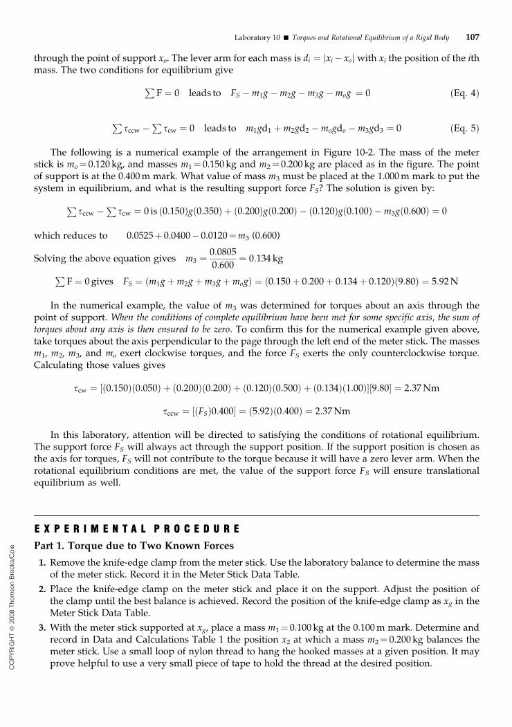
through the point of support xo. The lever arm for each mass is di ¼ jxi � xoj with xi the position of the ithmass. The two conditions for equilibrium give
PF ¼ 0 leads to FS �m1g�m2g�m3g�mog ¼ 0 ðEq: 4Þ
Ptccw �P tcw ¼ 0 leads to m1gd1 þm2gd2 �mogdo �m3gd3 ¼ 0 ðEq: 5Þ
The following is a numerical example of the arrangement in Figure 10-2. The mass of the meterstick is mo¼ 0.120 kg, and masses m1¼ 0.150 kg and m2¼ 0.200 kg are placed as in the figure. The pointof support is at the 0.400m mark. What value of mass m3 must be placed at the 1.000m mark to put thesystem in equilibrium, and what is the resulting support force FS? The solution is given by:
Ptccw �P tcw ¼ 0 is ð0:150Þgð0:350Þ þ ð0:200Þgð0:200Þ � ð0:120Þgð0:100Þ �m3gð0:600Þ ¼ 0
which reduces to 0.0525þ 0.0400� 0.0120¼m3 (0.600)
Solving the above equation gives m3 ¼ 0:0805
0:600¼ 0:134 kg
PF ¼ 0 gives FS ¼ ðm1gþm2gþm3gþmogÞ ¼ ð0:150þ 0:200þ 0:134þ 0:120Þð9:80Þ ¼ 5:92N
In the numerical example, the value of m3 was determined for torques about an axis through thepoint of support. When the conditions of complete equilibrium have been met for some specific axis, the sum oftorques about any axis is then ensured to be zero. To confirm this for the numerical example given above,take torques about the axis perpendicular to the page through the left end of the meter stick. The massesm1, m2, m3, and mo exert clockwise torques, and the force FS exerts the only counterclockwise torque.Calculating those values gives
tcw ¼ ½ð0:150Þð0:050Þ þ ð0:200Þð0:200Þ þ ð0:120Þð0:500Þ þ ð0:134Þð1:00Þ�½9:80� ¼ 2:37Nm
tccw ¼ ½ðFSÞ0:400� ¼ ð5:92Þð0:400Þ ¼ 2:37Nm
In this laboratory, attention will be directed to satisfying the conditions of rotational equilibrium.The support force FS will always act through the support position. If the support position is chosen asthe axis for torques, FS will not contribute to the torque because it will have a zero lever arm. When therotational equilibrium conditions are met, the value of the support force FS will ensure translationalequilibrium as well.
E X P E R I M E N T A L P R O C E D U R EPart 1. Torque due to Two Known Forces
1. Remove the knife-edge clamp from the meter stick. Use the laboratory balance to determine the massof the meter stick. Record it in the Meter Stick Data Table.
2. Place the knife-edge clamp on the meter stick and place it on the support. Adjust the position ofthe clamp until the best balance is achieved. Record the position of the knife-edge clamp as xg in theMeter Stick Data Table.
3. With the meter stick supported at xg, place a mass m1¼ 0.100 kg at the 0.100m mark. Determine andrecord in Data and Calculations Table 1 the position x2 at which a mass m2¼ 0.200 kg balances themeter stick. Use a small loop of nylon thread to hang the hooked masses at a given position. It mayprove helpful to use a very small piece of tape to hold the thread at the desired position.
COPYRIG
HTª
2008ThomsonBrooks/Cole
Laboratory 10 n Torques and Rotational Equilibrium of a Rigid Body 107

4. Calculate the lever arm for each force di ¼ jxg � xijwhere xi is the position of the ith mass. With thesupport at the position xg, the meter stick mass has zero lever arm and contributes no torque. Recordthe values of d1 and d2 in Data and Calculations Table 1.
5. Calculate and record in Data and Calculations Table 1 the value of the torques. The only counter-clockwise torque is due to m1 and
Ptccw¼m1gd1. The only clockwise torque is due to m2 andP
tcw¼m2gd2. Use a value of 9.80m/s2 for g for these and all other calculations.
6. Calculate the percentage difference betweenP
tccw andP
tcw and record it in Data and CalculationsTable 1.
Part 2. Torque due to Three Known Forces
1. Support the meter stick at xg. Place m1¼ 0.100 kg at 0.100m, and m2¼ 0.200 kg at 0.750m. Determinethe position x3 at which m3¼ 0.050 kg balances the system. Record the value of x3 in Data andCalculations Table 2.
2. The meter stick mass mo makes no contribution to the torque. Calculate the lever arm for each of themasses and record the values in Data and Calculations Table 2. (di ¼ jxg � xij)
3. Calculate the values ofP
tccw andP
tcw and record them in Data and Calculations Table 2.
4. Calculate the percentage difference betweenP
tccw andP
tcw and record it in Data and CalculationsTable 2.
Part 3. Determination of the Meter Stick Mass by Torques
1. Place a mass m1¼ 0.200 kg at the 0.100m position. Loosen the knife-edge clamp and slide the meterstick in the clamp until the torque exerted by m1g is balanced by the torque of the meter stick weightacting at xg. When the best balance is achieved, tighten the clamp. The position at which the meterstick is supported is xo. Record xo in Data and Calculations Table 3.
2. The values of the lever arms are given by d1 ¼ jx1 � xoj and do ¼ jxg � xoj. Calculate and record thevalues of d1 and do in Data and Calculations Table 3.
3. For these conditions,P
tccw¼m1gd1 andP
tcw¼mogdo where mo stands for the assumed unknownmass of the meter stick. Equating the two torques gives mo¼m1(d1/do). Calculate and record in Dataand Calculations Table 3 this value as (mo)exp.
4. Calculate and record in Data and Calculations Table 3 the percentage error in (mo)exp compared to themeter stick mass determined by the laboratory balance.
Part 4. Comparison of Experimental and Theoretical Determinations of the Location of anApplied Force
1. Adjust the knife-edge clamp to the 0.400m mark. Place m1¼ 0.050 kg at 0.050m, m2¼ 0.300 kg at0.300m, and m3¼ 0.200 kg at 0.700m as shown in Figure 10-3. With the meter stick supported at the0.400m mark, determine the position at which massm4¼ 0.100 kg balances the meter stick. Record this
2010
m1
30 40
??
50 60 70 80 90
m2
m4
m3
Figure 10-3 The location of mass m4 needed to place the system in equilibrium is to be determined bothexperimentally and theoretically, and then compared.
108 Physics Laboratory Manual n Loyd
position as x4 in Data and Calculations Table 4 and use this value of x4 to calculate the lever arm d4 andrecord it in Data and Calculations Table 4 as (d4)exp.
2. In the space provided in Data and Calculations Table 4, write the equation for the rotationalequilibrium with counterclockwise torques positive and clockwise torques negative. Use m1, m2, m3,and m4 as the symbols for the appropriate mass, and d1, d2, d3, and d4 as the symbols for the leverarms. Include the contribution from the meter stick mass mo acting at the center of gravity of themeter stick xg.
3. In the equation, treat the lever arm d4 of mass m4 as unknown and all the other quantities as known.Solve the equation to obtain a value for d4 and record that result in Data and Calculations Table 4 as(d4)theo.
4. Calculate the percentage error in (d4)exp compared to (d4)theo and record it in Data and CalculationsTable 4.
Part 5. Determination of an Unknown Mass by Torques
1. Use an experimental arrangement with the meter stick that is similar to those that we have used thusfar to devise a method to determine the mass of an unknown mass. Describe carefully the procedurethat is followed. Use at least one known mass and state its value and location on the meter stick.Write an equation that describes the equilibrium of the system treating the mass as unknown.Include a sketch of the experimental arrangement showing the position of all masses known andunknown. Construct your own Data and Calculations Table 5 listing all the relevant quantities.
2. Use the laboratory balance to determine the value of the unknown mass. Calculate the percentageerror in your experimental value of the unknownmass compared to that obtained using the laboratorybalance.
COPYRIG
HTª
2008ThomsonBrooks/Cole
Laboratory 10 n Torques and Rotational Equilibrium of a Rigid Body 109

This page intentionally left blank
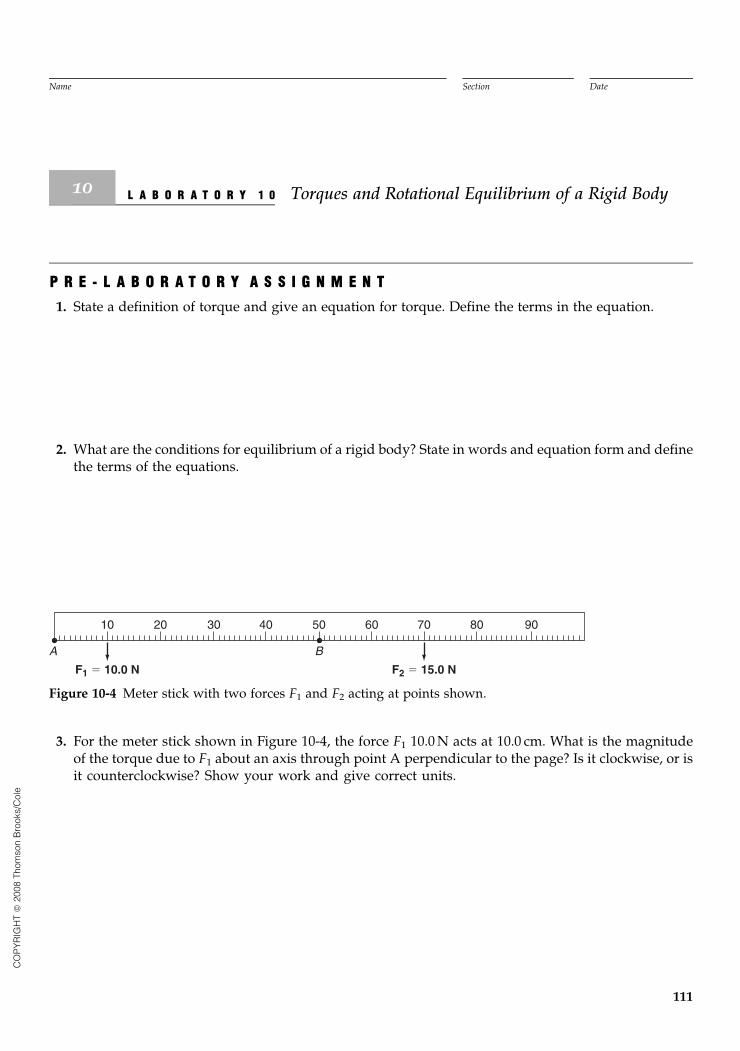
Name . . . . . . . . . . . . . . . . . . . . . . . . . . . . . . . . . . . . . . . . . . . . . . . . . . . . . . . . . . . . . . . . . . . . . . . . . Section . . . . . . . . . . . . . . . . Date . . . . . . . . . . . . . . . .
10 L A B O R A T O R Y 1 0 Torques and Rotational Equilibrium of a Rigid Body
P R E - L A B O R A T O R Y A S S I G N M E N T1. State a definition of torque and give an equation for torque. Define the terms in the equation.
2. What are the conditions for equilibrium of a rigid body? State in words and equation form and definethe terms of the equations.
3. For the meter stick shown in Figure 10-4, the force F1 10.0N acts at 10.0 cm. What is the magnitudeof the torque due to F1 about an axis through point A perpendicular to the page? Is it clockwise, or isit counterclockwise? Show your work and give correct units.
COPYRIG
HTª
2008ThomsonBrooks/Cole
20
F1 � 10.0 N F2 � 15.0 N
10
A B
30 40 50 60 70 80 90
Figure 10-4 Meter stick with two forces F1 and F2 acting at points shown.
111

4. In Figure 10-4 the force F2¼ 15.0N acts at the point 70.0 cm. What is the magnitude of the torque dueto F2 about an axis through point B and perpendicular to the page? Is the torque clockwise, or is itcounterclockwise? Show your work and give correct units.
5. For the meter stick in Figure 10-4, what is the magnitude of the net torque due to both forces F1 andF2 about an axis perpendicular to the page through point A? Is it clockwise or counterclockwise?Show your work.
6. In Figure 10-5 if mass m1¼ 0.100 kg acts at 20.0 cm, what is the value of mass m2 that must be placedat the position 70.0 cm shown to put the system in equilibrium?Write the equation for
Ptccw¼P tcw
with the mass m2 as unknown and solve for m2. Assume that the meter stick is uniform andsymmetric. Show your work.
2010 30 40 50 60 70 80 90
m1 m2
Figure 10-5 Meter stick with forces applied by hanging two masses m1 and m2.
112 Physics Laboratory Manual n Loyd

Name . . . . . . . . . . . . . . . . . . . . . . . . . . . . . . . . . . . . . . . . . . . . . . . . . . . . . . . . . . . . . . . . . . . . . . . . . Section . . . . . . . . . . . . . . . . Date . . . . . . . . . . . . . . . .
Lab Partners . . . . . . . . . . . . . . . . . . . . . . . . . . . . . . . . . . . . . . . . . . . . . . . . . . . . . . . . . . . . . . . . . . . . . . . . . . . . . . . . . . . . . . . . . . . . . . . . . . . . . . . . . . . . . . . . . . . .
10 L A B O R A T O R Y 1 0 Torques and Rotational Equilibrium of a Rigid Body
L A B O R A T O R Y R E P O R T
Data and Calculations Table 3
Support Position xo ¼ m
Mass (kg) Position (m) Lever arm (m) (mo)exp¼ kg % Error
m1¼ 0.200 x1¼ 0.100 d1¼
mo¼ xg do¼
COPYRIG
HTª
2008ThomsonBrooks/Cole
Meter Stick Data Table
mo ¼ kg xg ¼ m
Data and Calculations Table 1
Mass (kg) Position (m) Lever arm (m) Torque (N�m) % Difference
m1¼ 0.100 x1¼ 0.100 d1¼ tccw¼
m2¼ 0.200 x2¼ d2¼ tcw¼
Data and Calculations Table 2
Mass (kg) Position (m) Lever arm (m) Torque (N�m) % Difference
m1¼ 0.100 x1¼ 0.100 d1¼ tccw¼m2¼ 0.200 x2¼ 0.750 d2¼
m3¼ 0.050 x3¼ d3¼ tcw¼
113

Data and Calculations Table 4
Support Position xo¼ 0.400m
Mass (kg) Position (m) Lever Arm (m) Equation for the Torque
m1¼ 0.050 x1¼ 0.050 d1¼
m2¼ 0.300 x2¼ 0.300 d2¼
m3¼ 0.200 x3¼ 0.700 d3¼ Solving equation for d4 gives(d4)theo ¼ m
m4¼ 0.100 x4¼ (d4)exp¼
mo¼ xg¼ do¼
Data and Calculations Table 5
114 Physics Laboratory Manual n Loyd

S A M P L E C A L C U L A T I O N S1. di ¼ jxi� xoj ¼
2.P
tccw¼
3.P
tcw¼
4. % Diff torques ¼ jtccw � tcwj=�0:5ðtccw þ tcwÞ
�� 100% ¼
5. (mo)exp¼m1(d1/do)¼
6. % Error for ðmoÞexp ¼ jE�Kj=K� 100% ¼
7. (d4)theo ¼
8. % Error for ðd4Þtheo ¼ jE�Kj=K� 100% ¼
9. Calculation for mexp in Part 5¼
10. % Error for mexp ¼ jE�Kj=K� 100% ¼
Q U E S T I O N S1. Consider the percentage difference between the
Ptccw and the
Ptcw for the first two parts of the
laboratory when known forces are balanced. A difference of 0.5% or less is excellent, a difference of1.0% or less is good, and a difference of 2% or less is acceptable. Based on these criteria, describe yourresults for the first two parts of the laboratory and defend your statement.
2. Using the same criteria as in Question 1 for the percentage differences, describe your results forthe determination of mass of the meter stick in Part 3 of the laboratory and for the determinationof the lever arm of the mass m4 in Part 4 of the laboratory.
COPYRIG
HTª
2008ThomsonBrooks/Cole
Laboratory 10 n Torques and Rotational Equilibrium of a Rigid Body 115

3. In all of the experimental arrangements the mass of the knife-edge clamp is ignored. Is this anapproximation because its mass is small, or is there some reason it makes no contribution to thetorque? State your reasoning clearly.
4. Suppose an experimental arrangement like the one in Part 2 has mass m1¼ 0.200 kg at the 0.100-mmark and a mass m2¼ 0.100 kg at the 0.750-m mark. Can the system be put in equilibrium by a0.050-kg mass? If it can be done, state where it would be placed. If it cannot be done, state why not.
5. In Part 1 of the laboratory, what is the value of the force Fs with which the support pushes upward onthe meter stick?
6. For the equilibrium conditions established in Part 4 of the laboratory, calculate the counterclockwiseand clockwise torques about an axis perpendicular to the page through a point at the left end of themeter stick. Calculate the percentage difference between the net counterclockwise torque and the netclockwise torque.
116 Physics Laboratory Manual n Loyd

Conservation of Energyon the Air Table
O B J E C T I V E So Determine the value of the spring constant k for two springs.
o Investigate how the speed, kinetic energy, and total spring potential energy of a puck on ahorizontal air table vary with time.
o Evaluate the extent to which the total mechanical energy (sum of kinetic energy plus springpotential energy) is constant as a function of position of the puck.
E Q U I P M E N T L I S T. Air table, sparktimer, air pump, foot switch, carbon paper, and recording paper
. Level, two springs, two spring clamps, and a double hook for the puck
. Meter stick, pulley, string, calibrated masses, and laboratory balance
T H E O R YThe force F exerted by a spring as it is elongated from its natural length xo to some greater length x isgiven by
F ¼ �kðx� xoÞ ðEq: 1Þ
where k is a constant called the spring constant. The spring constant is defined as the force per unitelongation and has units of N/m. The value of k will be different for each spring depending upon thespring material properties and how tightly the spring is wound. The value of k for a spring is determinedby measuring the elongation caused by a known force.
The force exerted by a spring is an example of a class of forces known as conservative forces. A con-servative force is one for which a potential energy function can be defined. For a spring force the potentialenergy U is given by
U ¼ ½ kðx� xoÞ2 ðEq: 2Þ
Physics Laboratory Manual n Loyd L A B O R A T O R Y 11
COPYRIG
HTª
2008ThomsonBrooks/Cole
117
ª 2008 Thomson Brooks/Cole, a part of TheThomson Corporation.Thomson, the Star logo, and Brooks/Cole are trademarks used herein under license. ALL RIGHTSRESERVED.No part of this workcovered by the copyright hereonmay be reproduced or used in any form or by any meansçgraphic, electronic, ormechanical, including photocopying, recording, taping,web distribution, informationstorage and retrieval systems,or in any othermannerçwithout the written permission of the publisher.
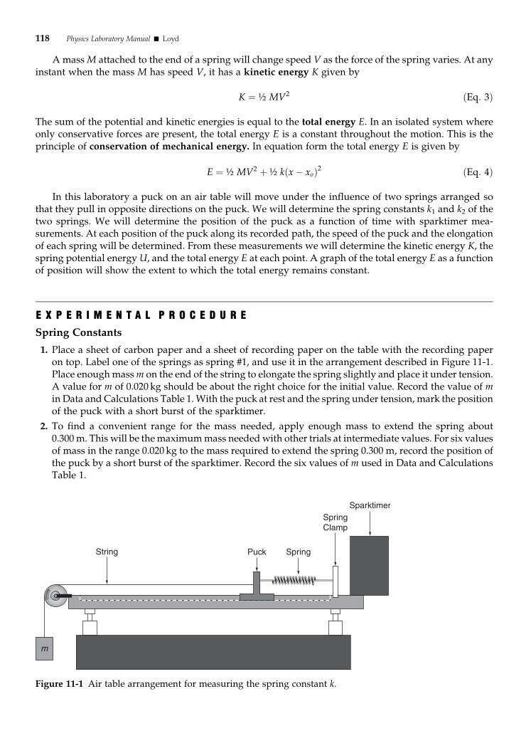
AmassM attached to the end of a spring will change speed V as the force of the spring varies. At anyinstant when the mass M has speed V, it has a kinetic energy K given by
K ¼ ½ MV2 ðEq: 3Þ
The sum of the potential and kinetic energies is equal to the total energy E. In an isolated system whereonly conservative forces are present, the total energy E is a constant throughout the motion. This is theprinciple of conservation of mechanical energy. In equation form the total energy E is given by
E ¼ ½ MV2 þ½ kðx� xoÞ2 ðEq: 4Þ
In this laboratory a puck on an air table will move under the influence of two springs arranged sothat they pull in opposite directions on the puck. We will determine the spring constants k1 and k2 of thetwo springs. We will determine the position of the puck as a function of time with sparktimer mea-surements. At each position of the puck along its recorded path, the speed of the puck and the elongationof each spring will be determined. From these measurements we will determine the kinetic energy K, thespring potential energyU, and the total energy E at each point. A graph of the total energy E as a functionof position will show the extent to which the total energy remains constant.
E X P E R I M E N T A L P R O C E D U R ESpring Constants
1. Place a sheet of carbon paper and a sheet of recording paper on the table with the recording paperon top. Label one of the springs as spring #1, and use it in the arrangement described in Figure 11-1.Place enoughmassm on the end of the string to elongate the spring slightly and place it under tension.A value for m of 0.020 kg should be about the right choice for the initial value. Record the value of min Data and Calculations Table 1.With the puck at rest and the spring under tension, mark the positionof the puck with a short burst of the sparktimer.
2. To find a convenient range for the mass needed, apply enough mass to extend the spring about0.300m. This will be themaximummass neededwith other trials at intermediate values. For six valuesof mass in the range 0.020 kg to the mass required to extend the spring 0.300 m, record the position ofthe puck by a short burst of the sparktimer. Record the six values of m used in Data and CalculationsTable 1.
m
String Puck Spring
SpringClamp
Sparktimer
Figure 11-1 Air table arrangement for measuring the spring constant k.
118 Physics Laboratory Manual n Loyd
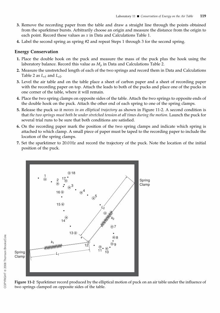
3. Remove the recording paper from the table and draw a straight line through the points obtainedfrom the sparktimer bursts. Arbitrarily choose an origin and measure the distance from the origin toeach point. Record these values as x in Data and Calculations Table 1.
4. Label the second spring as spring #2 and repeat Steps 1 through 3 for the second spring.
Energy Conservation
1. Place the double hook on the puck and measure the mass of the puck plus the hook using thelaboratory balance. Record this value as Mp in Data and Calculations Table 2.
2. Measure the unstretched length of each of the two springs and record them in Data and CalculationsTable 2 as Lo1 and Lo2.
3. Level the air table and on the table place a sheet of carbon paper and a sheet of recording paperwith the recording paper on top. Attach the leads to both of the pucks and place one of the pucks inone corner of the table, where it will remain.
4. Place the two spring clamps on opposite sides of the table. Attach the two springs to opposite ends ofthe double hook on the puck. Attach the other end of each spring to one of the spring clamps.
5. Release the puck so it moves in an elliptical trajectory as shown in Figure 11-2. A second condition isthat the two springs must both be under stretched tension at all times during the motion. Launch the puck forseveral trial runs to be sure that both conditions are satisfied.
6. On the recording paper mark the position of the two spring clamps and indicate which spring isattached to which clamp. A small piece of paper must be taped to the recording paper to include thelocation of the spring clamps.
7. Set the sparktimer to 20.0Hz and record the trajectory of the puck. Note the location of the initialposition of the puck.
COPYRIG
HTª
2008ThomsonBrooks/Cole
2 17
18
34
5
SpringClamp
SpringClamp
1011
9
8
7
13
12k1
k2
16
15
14
L2
L1
1
Figure 11-2 Sparktimer record produced by the elliptical motion of puck on an air table under the influence oftwo springs clamped on opposite sides of the table.
Laboratory 11 n Conservation of Energy on the Air Table 119
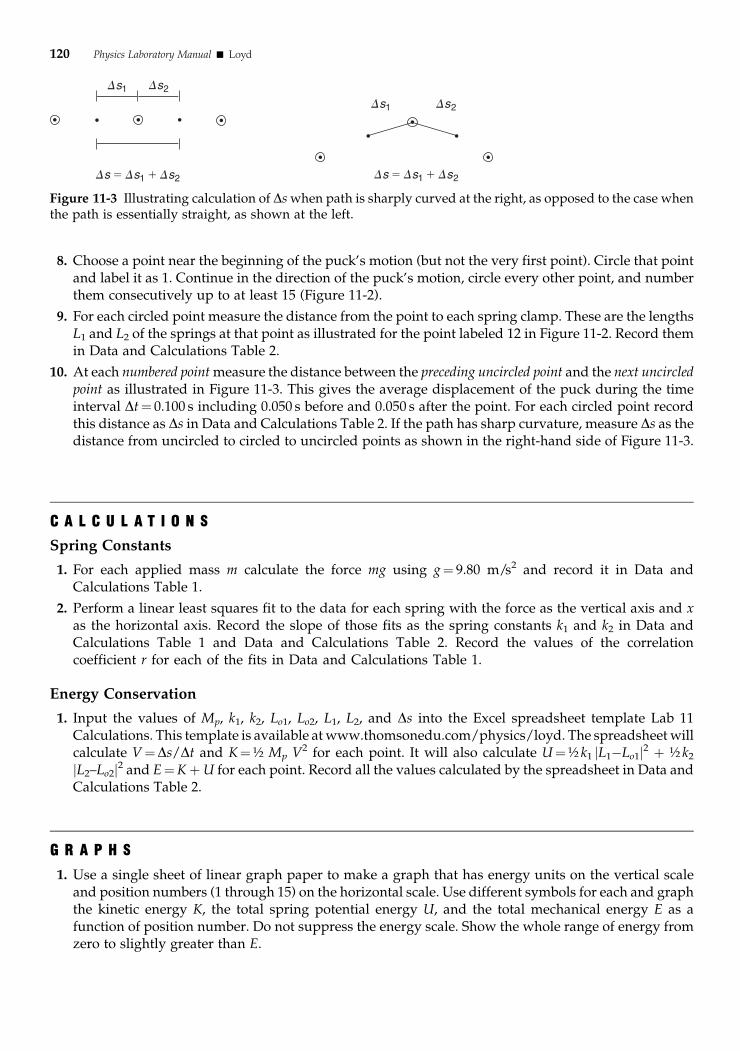
8. Choose a point near the beginning of the puck’s motion (but not the very first point). Circle that pointand label it as 1. Continue in the direction of the puck’s motion, circle every other point, and numberthem consecutively up to at least 15 (Figure 11-2).
9. For each circled point measure the distance from the point to each spring clamp. These are the lengthsL1 and L2 of the springs at that point as illustrated for the point labeled 12 in Figure 11-2. Record themin Data and Calculations Table 2.
10. At each numbered pointmeasure the distance between the preceding uncircled point and the next uncircledpoint as illustrated in Figure 11-3. This gives the average displacement of the puck during the timeinterval Dt¼ 0.100 s including 0.050 s before and 0.050 s after the point. For each circled point recordthis distance as Ds in Data and Calculations Table 2. If the path has sharp curvature, measure Ds as thedistance from uncircled to circled to uncircled points as shown in the right-hand side of Figure 11-3.
C A L C U L A T I O N SSpring Constants
1. For each applied mass m calculate the force mg using g¼ 9.80 m/s2 and record it in Data andCalculations Table 1.
2. Perform a linear least squares fit to the data for each spring with the force as the vertical axis and xas the horizontal axis. Record the slope of those fits as the spring constants k1 and k2 in Data andCalculations Table 1 and Data and Calculations Table 2. Record the values of the correlationcoefficient r for each of the fits in Data and Calculations Table 1.
Energy Conservation
1. Input the values of Mp, k1, k2, Lo1, Lo2, L1, L2, and Ds into the Excel spreadsheet template Lab 11Calculations. This template is available atwww.thomsonedu.com/physics/loyd. The spreadsheetwillcalculate V¼Ds/Dt and K¼½ Mp V2 for each point. It will also calculate U¼½ k1 jL1�Lo1j2 þ ½ k2jL2–Lo2j2 and E¼KþU for each point. Record all the values calculated by the spreadsheet in Data andCalculations Table 2.
G R A P H S1. Use a single sheet of linear graph paper to make a graph that has energy units on the vertical scale
and position numbers (1 through 15) on the horizontal scale. Use different symbols for each and graphthe kinetic energy K, the total spring potential energy U, and the total mechanical energy E as afunction of position number. Do not suppress the energy scale. Show the whole range of energy fromzero to slightly greater than E.
�s1
�s � �s1 � �s2 �s � �s1 � �s2
�s2
�s1 �s2
Figure 11-3 Illustrating calculation of Dswhen path is sharply curved at the right, as opposed to the case whenthe path is essentially straight, as shown at the left.
120 Physics Laboratory Manual n Loyd

Name . . . . . . . . . . . . . . . . . . . . . . . . . . . . . . . . . . . . . . . . . . . . . . . . . . . . . . . . . . . . . . . . . . . . . . . . . Section . . . . . . . . . . . . . . . . Date . . . . . . . . . . . . . . . .
11 L A B O R A T O R Y 1 1 Conservation of Energy on the Air Table
P R E - L A B O R A T O R Y A S S I G N M E N T1. What is the definition, both in words and equation form, of the spring constant k? What are the units
of k?
2. What is the equation for the spring potential energy of a spring? Define all terms used in the equation.
3. What is the principle of conservation of mechanical energy applied to a massm attached to a spring ofspring constant k? State it in words and equation form and define all terms used.
4. What kinds of forces conserve mechanical energy? Is mechanical energy conserved if frictional forcesare present?
COPYRIG
HTª
2008ThomsonBrooks/Cole
121
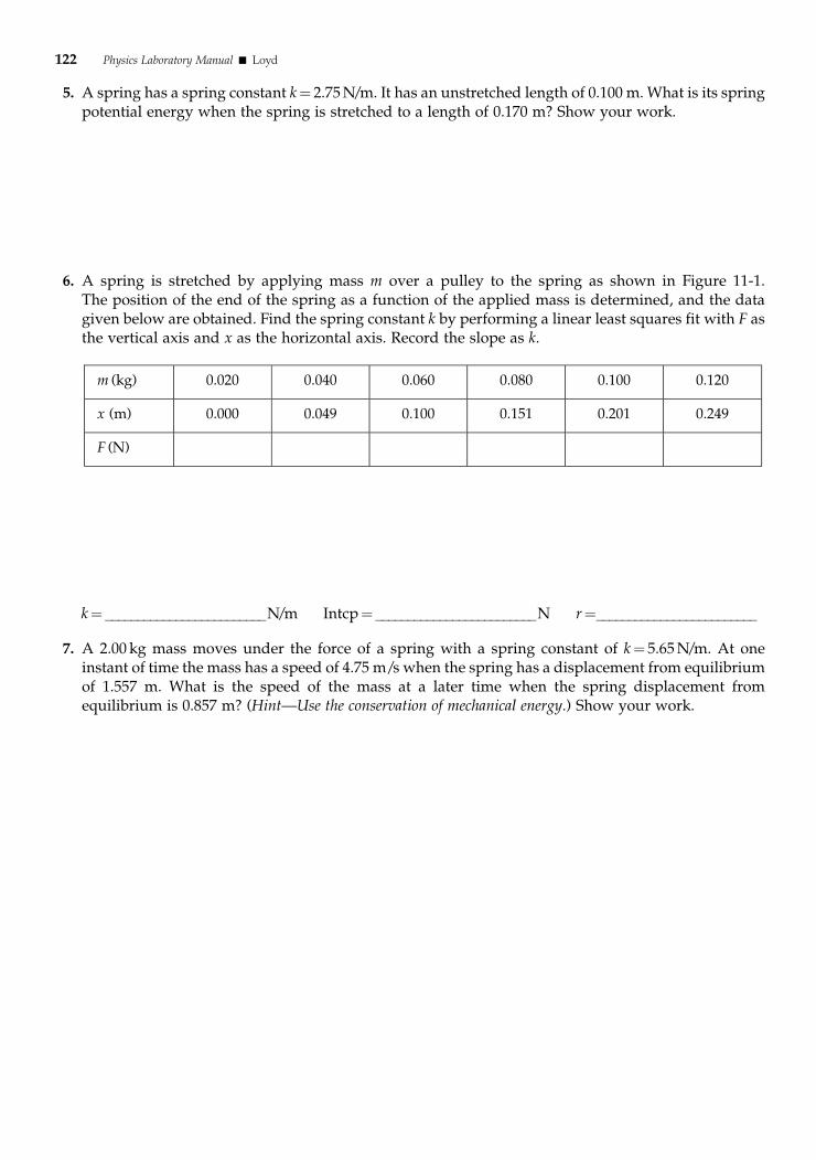
5. A spring has a spring constant k¼ 2.75N/m. It has an unstretched length of 0.100 m. What is its springpotential energy when the spring is stretched to a length of 0.170 m? Show your work.
6. A spring is stretched by applying mass m over a pulley to the spring as shown in Figure 11-1.The position of the end of the spring as a function of the applied mass is determined, and the datagiven below are obtained. Find the spring constant k by performing a linear least squares fit with F asthe vertical axis and x as the horizontal axis. Record the slope as k.
m (kg) 0.020 0.040 0.060 0.080 0.100 0.120
x (m) 0.000 0.049 0.100 0.151 0.201 0.249
F (N)
k¼ _________________________N/m Intcp¼ _________________________N r¼_________________________
7. A 2.00 kg mass moves under the force of a spring with a spring constant of k¼ 5.65N/m. At oneinstant of time the mass has a speed of 4.75 m/s when the spring has a displacement from equilibriumof 1.557 m. What is the speed of the mass at a later time when the spring displacement fromequilibrium is 0.857 m? (Hint—Use the conservation of mechanical energy.) Show your work.
122 Physics Laboratory Manual n Loyd

Name . . . . . . . . . . . . . . . . . . . . . . . . . . . . . . . . . . . . . . . . . . . . . . . . . . . . . . . . . . . . . . . . . . . . . . . . . Section . . . . . . . . . . . . . . . . Date . . . . . . . . . . . . . . . .
Lab Partners . . . . . . . . . . . . . . . . . . . . . . . . . . . . . . . . . . . . . . . . . . . . . . . . . . . . . . . . . . . . . . . . . . . . . . . . . . . . . . . . . . . . . . . . . . . . . . . . . . . . . . . . . . . . . . . . . . . .
11 L A B O R A T O R Y 1 1 Conservation of Energy on the Air Table
L A B O R A T O R Y R E P O R T
COPYRIG
HTª
2008ThomsonBrooks/Cole
Data and Calculations Table 1
Spring 1 k1¼ N/m
Point m (kg) mg (N) x (m)
1
2
3
4
5
6
r¼
Spring 2 k2¼ N/m
Point m (kg) mg (N) x (m)
1
2
3
4
5
6
r¼
123

S A M P L E C A L C U L A T I O N S1. F¼mg¼2. Velocity¼V¼Ds/Dt¼3. K¼½ MpV
2¼4. U¼½ k1 jL1�Lo1j2þ½ k2 jL2�Lo2j2¼5. E¼KþU¼
Data and Calculations Table 2
Mp¼ kg k1¼ N/m k2¼ N/m Lo1¼ m Lo2¼ m
Point L1 (m) L2 (m) Ds (m) V (m/s) K (J) U (J) E (J)
1
2
3
4
5
6
7
8
9
10
11
12
13
14
15
124 Physics Laboratory Manual n Loyd
Q U E S T I O N S1. Calculate the mean and standard error for the 15 values for the total energy E. Divide the standard
error by the mean, and express the ratio as a percentage. Use this calculation as evidence for yourstatement of how constant are your values of E.
2. Although your values of E should be fairly constant, they normally show a slight decrease frombeginning to end of the data caused by friction. Calculate the decrease in E from the first to last point.Also calculate the total path lengthof thepuckby summing the values ofDs. Divide the loss in energybythe total path length, which is the force of friction. What is the friction for your data? Show your work.
3. In the determination of the spring constant k the origin from which the position x was measured waschosen arbitrarily. Would choosing another point for the origin significantly change the valueobtained for k? State clearly the reasoning for your answer.
4. Summarize in your own words the physical theory that this laboratory is supposed to demonstrate.Do your results support the theory? Consider the variations in the values of U, K, and E to supportyour answer.
COPYRIG
HTª
2008ThomsonBrooks/Cole
Laboratory 11 n Conservation of Energy on the Air Table 125

This page intentionally left blank
Conservation of Springand GravitationalPotential Energy
O B J E C T I V E So Determine the value of the spring constant k for a spring.
o Investigate the change in gravitational energy DUg¼mg(xf� xi) and the change in springpotential energy DUk ¼ ð½Þkðx2f�x2i Þ for a mass suspended from the spring.
o Evaluate the extent to which the changes in energy are equal as the mass oscillates.
E Q U I P M E N T L I S T. Spring in the form of a truncated cone made of spring brass with a spring constant of about 10N/m.(Available from Central Scientific Co. If another spring is used, appropriate adjustments should bemade in the masses and distances used.)
. Set of calibrated hooked masses
. Table clamp, right angle clamps, support rods, meter stick
T H E O R YWhen a spring is stretched or compressed a distance x from its equilibrium length, the spring exerts arestoring force F. The equation relating the force F and the displacement x is
F ¼ �kx ðEq: 1Þ
and k is a constant called the spring constant with unitsN/m. The negative sign in Equation 1 indicatesthat the restoring force direction is opposite the displacement.
When a spring is compressed or stretched by x it has stored energy called spring potential energygiven by Uk¼½ kx2. When the spring is stretched from a displacement of x1 to a displacement of x2 thechange in spring energy is equal to the work done on the spring (Figure 12-1).
Work ¼ DUk ¼ ½ kðx22 � x21Þ ðEq: 2Þ
Physics Laboratory Manual n Loyd L A B O R A T O R Y 12
COPYRIG
HTª
2008ThomsonBrooks/Cole
127
ª 2008 Thomson Brooks/Cole, a part of TheThomson Corporation.Thomson, the Star logo, and Brooks/Cole are trademarks used herein under license. ALL RIGHTSRESERVED.No part of this workcovered by the copyright hereonmay be reproduced or used in any form or by any meansçgraphic, electronic, ormechanical, including photocopying, recording, taping,web distribution, informationstorage and retrieval systems,or in any othermannerçwithout the written permission of the publisher.

A spring with spring constant k is supported at the top by a rigid support and allowed to hangvertically. The vertical position at which the lower end of the spring hangs is the zero of the coordinate x.A hooked mass m is placed by hand on the end of the spring, and the mass is slowly lowered by hand.The mass will extend the spring by an amount xo when the hand is removed as shown in Figure 12-1.
The mass is raised and supported by hand with the lower end of the spring at position x1 aboveposition xo as shown in Figure 12-1. The mass is now released and allowed to fall under the influenceof the spring and the earth’s gravitational force. The mass will fall to its lowest point with displacementx2 and then rebound and oscillate.
The gravitational potential energy relative to any horizontal plane is mgx where x is the distanceabove the plane. The total mechanical energy of the system is the sum of kinetic energy, spring potentialenergy, and gravitational potential energy. Consider the total mechanical energy at x1 and x2. At eachof these points the kinetic energy is zero, and the total mechanical energy is the sum of the springpotential energy and the gravitational potential energy. The center of mass of m is distance d below thelower end of the spring, and the gravitational potential energy zero is the same as the equilibrium point ofthe spring. The equation for the sum of spring energy and gravitational energy is
½ kx21 �mgðx1 þ dÞ ¼ ½ kx22 �mgðx2 þ dÞ ðEq: 3Þ
or ½ kx21 �mgx1 ¼ ½ kx22 �mgx2 ðEq: 4Þ
Both gravitational potential energy terms are negative because the mass is below the reference point forboth positions. Equation 4 can be rewritten as
mgðx2 � x1Þ ¼ ½ kðx22 � x21Þ ðEq: 5Þ
Equation 5 states that the change in gravitational energy between points 1 and 2 is equal to the change inspring potential energy between those points because the kinetic energy is zero at both points 1 and 2.This laboratory will consist of a series of measurements that will test the validity of Equation 5.
E X P E R I M E N T A L P R O C E D U R ESpring Constant
1. Use appropriate clamps and rods to provide a horizontal rod sticking out beyond the table as shownin Figure 12-2. Hang the spring on the horizontal rod, and attach it to the rod with a piece of tape.
m
m
x � 0
x0x1
m
x2
Figure 12-1 Positions of a mass m on a spring in the earth’s gravitational field.
128 Physics Laboratory Manual n Loyd
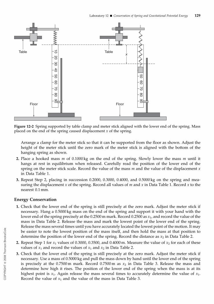
Arrange a clamp for the meter stick so that it can be supported from the floor as shown. Adjust theheight of the meter stick until the zero mark of the meter stick is aligned with the bottom of thehanging spring as shown.
2. Place a hooked mass m of 0.1000 kg on the end of the spring. Slowly lower the mass m until ithangs at rest in equilibrium when released. Carefully read the position of the lower end of thespring on the meter stick scale. Record the value of the mass m and the value of the displacement xin Data Table 1.
3. Repeat Step 2, placing in succession 0.2000, 0.3000, 0.4000, and 0.5000 kg on the spring and mea-suring the displacement x of the spring. Record all values of m and x in Data Table 1. Record x to thenearest 0.1mm.
Energy Conservation
1. Check that the lower end of the spring is still precisely at the zero mark. Adjust the meter stick ifnecessary. Hang a 0.5000 kg mass on the end of the spring and support it with your hand with thelower end of the spring precisely at the 0.2500mmark. Record 0.2500 as x1, and record the value of themass in Data Table 2. Release the mass and mark the lowest point of the lower end of the spring.Release the mass several times until you have accurately located the lowest point of the motion. It maybe easier to note the lowest position of the mass itself, and then hold the mass at that position todetermine the position of the lower end of the spring. Record the distance as x2 in Data Table 2.
2. Repeat Step 1 for x1 values of 0.3000, 0.3500, and 0.4000m. Measure the value of x2 for each of thesevalues of x1 and record the values of x1 and x2 in Data Table 2.
3. Check that the lower end of the spring is still precisely at the zero mark. Adjust the meter stick ifnecessary. Use a mass of 0.5000 kg and pull the mass down by hand until the lower end of the springis precisely at the 0.7500m mark. Record 0.7500m as x2 in Data Table 3. Release the mass anddetermine how high it rises. The position of the lower end of the spring when the mass is at itshighest point is x1. Again release the mass several times to accurately determine the value of x1.Record the value of x1 and the value of the mass in Data Table 3.C
OPYRIG
HTª
2008ThomsonBrooks/Cole
9080
7060
50
9080
7060
5040
3020
10
Floor Floor
Tablex
Table
Figure 12-2 Spring supported by table clamp and meter stick aligned with the lower end of the spring. Massplaced on the end of the spring caused displacement x of the spring.
Laboratory 12 n Conservation of Spring and Gravitational Potential Energy 129

4. Repeat Step 3 for x2 values of 0.7000, 0.6500, and 0.6000m. Measure the value of x1 for each of thesevalues of x2 and record the values of x1 and x2 in Data Table 3.
C A L C U L A T I O N SSpring Constant
1. Calculate the force mg for each mass and record the values in Calculations Table 1. Use the valueof 9.800m/s2 for g.
2. Perform a linear least squares fit with mg as the vertical axis and x as the horizontal axis. Record theslope in Calculations Table 1 as the spring constant k and record r the correlation coefficient.
Energy Conservation
1. For each of the four measurements of the falling mass in Data Table 2, calculate the change in thegravitational potential energy DUg where DUg¼mg(x2� x1). Calculate the change in spring potentialenergy DUk where DUk ¼ ð1=2Þkðx22 � x21Þ. Record the results in Calculations Table 2.
2. Calculate the percentage differences between DUg and DUk for each case of Step 1 and record them inCalculations Table 2.
3. For each of the four measurements of the rising mass in Data Table 3, calculate the change ingravitational potential energy DUg and the change in spring potential energy DUk. Record the resultsin Calculations Table 3.
4. Calculate the percentage differences between DUg and DUk for each case of Step 3 and record them inCalculations Table 3.
G R A P H S1. Graph the data from Calculations Table 1 for force mg versus displacement x with mg as the ver-
tical axis and x as the horizontal axis. Also show on the graph the straight line obtained from the fitto the data.
130 Physics Laboratory Manual n Loyd
Name . . . . . . . . . . . . . . . . . . . . . . . . . . . . . . . . . . . . . . . . . . . . . . . . . . . . . . . . . . . . . . . . . . . . . . . . . Section . . . . . . . . . . . . . . . . Date . . . . . . . . . . . . . . . .
12 L A B O R A T O R Y 1 2 Conservation of Spring and GravitationalPotential Energy
P R E - L A B O R A T O R Y A S S I G N M E N T1. A spring has a spring constant of k¼ 7.50N/m. If the spring is displaced 0.550m from its equilibrium
position, what is the force that the spring exerts? Assume for this and for all other questions in the pre-laboratory that g¼ 9.80m/s2. Show your work.
2. A spring of spring constant k¼ 8.25N/m is displaced from equilibrium by a distance of 0.150m.What is the stored energy in the form of spring potential energy? Show your work.
3. A spring of spring constant k¼ 12.5N/m is hung vertically. A 0.500 kg mass is then suspended fromthe spring. What is the displacement of the end of the spring due to the weight of the 0.500 kg mass?Show your work.
4. A mass of 0.400 kg is raised by a vertical distance of 0.450m in the earth’s gravitational field. What isthe change in its gravitational potential energy? Show your work.
COPYRIG
HTª
2008ThomsonBrooks/Cole
131
5. A spring of spring constant k¼ 8.75N/m is hung vertically from a rigid support. A mass of 0.500 kgis placed on the end of the spring and supported by hand at a point so that the displacement of thespring is 0.250m. The mass is suddenly released and allowed to fall. At the lowest position of themass what is the displacement of the spring from its equilibrium position? (Hint—Apply Equation 5with x1¼ 0.250m and x2 the unknown. This will lead to a quadratic equation with one of the solu-tions the unknown x2, and the other solution the original 0.250m displacement.) Show your work.
6. The laboratory is based on the assumption that at the two points of the motion being considered,the mass is at rest. What kind of energy does not need to be included under these experimentalconditions?
132 Physics Laboratory Manual n Loyd

Name . . . . . . . . . . . . . . . . . . . . . . . . . . . . . . . . . . . . . . . . . . . . . . . . . . . . . . . . . . . . . . . . . . . . . . . . . Section . . . . . . . . . . . . . . . . Date . . . . . . . . . . . . . . . .
Lab Partners . . . . . . . . . . . . . . . . . . . . . . . . . . . . . . . . . . . . . . . . . . . . . . . . . . . . . . . . . . . . . . . . . . . . . . . . . . . . . . . . . . . . . . . . . . . . . . . . . . . . . . . . . . . . . . . . . . . .
12 L A B O R A T O R Y 1 2 Conservation of Spring and GravitationalPotential Energy
L A B O R A T O R Y R E P O R T
COPYRIG
HTª
2008ThomsonBrooks/Cole
Data Table 1
m (kg) x (m)
Calculations Table 1
mg (N) k (N/m) r
Data Table 2
x1 (m) x2 (m) m (kg)
Calculations Table 2
mg (x2� x1) (J) 1=2 k (x22 � x21) (J) % Diff
133
S A M P L E C A L C U L A T I O N S1. mg¼2. mg(x2� x1)¼3. 1=2 kðx22 � x21Þ ¼4. % Diff¼ 2(E1�E2)/(E1þE2)� 100%¼
Q U E S T I O N S1. For five data points, statistical theory states that there is only 0.1% probability that a value of r ‡ 0.992
would be obtained for uncorrelated data. Based on your value of r, make the best statement you canabout the extent to which your data indicate that the force and displacement are linear.
2. Describe the extent to which your data indicate that mechanical energy is conserved in this laboratory.Consider the percentage differences in the energy changes in Data Table 2 and Data Table 3 in youranswer.
Data Table 3
x1 (m) x2 (m) m (kg)
Calculations Table 3
mg (x2� x1) (J) 1=2 k (x22 � x21) (J) % Diff
134 Physics Laboratory Manual n Loyd
3. Examine your data in Data Table 2 and in Data Table 3. For the data with the smallest percentagedifference, compare the total energy at each point. Calculate the sum UkþUg at x1 as ½kx21�mgx1.Calculate that sum at x2 as ½kx22�mgx2. Do you expect them to agree reasonably well? Explain whythey should or should not be the same.
4. Consider the same data as used in Question 3. Calculate the value of x halfway between x1 and x2.Calculate UkþUg¼½kx2�mgx for that point. Do you expect them to agree with the energycalculated in Question 3? If they agree reasonably well, explain why they do. If they do not agree,explain why they do not agree.
COPYRIG
HTª
2008ThomsonBrooks/Cole
Laboratory 12 n Conservation of Spring and Gravitational Potential Energy 135

This page intentionally left blank
The Ballistic Pendulum andProjectile Motion
O B J E C T I V E So Investigate how the initial velocity of a ball fired into a ballistic pendulum is related to the initial
velocity with which the pendulum plus ball moves after the collision.
o Investigate the kinetic energy loss in the collision of the ball with the pendulum.
o Determine the initial velocity of the ball by firing it as a projectile and compare it with the velocitydetermined by the collision.
E Q U I P M E N T L I S T. Ballistic pendulum apparatus with projectile ball
. Laboratory balance and calibrated masses
. Meter stick, plain paper, carbon paper, and masking tape
T H E O R YBallistic Pendulum
The principle of conservation of momentum states that the total momentum of a system of particlesremains constant if there are no external forces acting on the system. Collision processes are goodexamples of this concept. In this laboratory we will use a ballistic pendulum to measure the velocity of aball projected by a spring gun. Figure 13-1 shows a ball of mass m moving initially in the horizontaldirection with speed vxo that then strikes a pendulum designed to catch the ball. The pendulum of massMcatches the ball and swings about pivot point O to some maximum height y2 above its original height y1.The system of ball plus pendulum rises a vertical distance of y2� y1 as a result of the process.
Momentum is conserved because the only forces acting on the ball and the pendulum in the directionof motion are the forces of the collision. The two particles stick together after the collision and move withthe same velocity V. A collision where particles stick together is called a completely inelastic collision.The equation for conservation of momentum is
mvxo ¼ ðmþMÞV ðEq: 1Þ
Physics Laboratory Manual n Loyd L A B O R A T O R Y 13
COPYRIG
HTª
2008ThomsonBrooks/Cole
137
ª 2008 Thomson Brooks/Cole, a part of TheThomson Corporation.Thomson, the Star logo, and Brooks/Cole are trademarks used herein under license. ALL RIGHTSRESERVED.No part of this workcovered by the copyright hereonmay be reproduced or used in any form or by any meansçgraphic, electronic, ormechanical, including photocopying, recording, taping,web distribution, informationstorage and retrieval systems,or in any othermannerçwithout the written permission of the publisher.
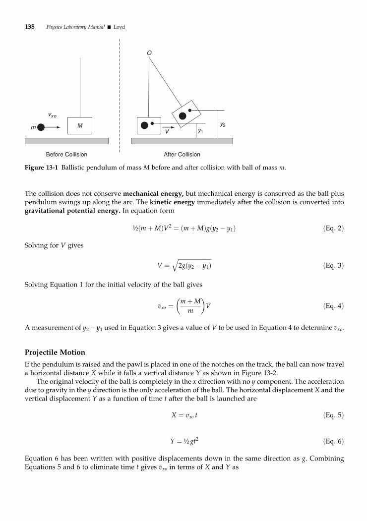
The collision does not conserve mechanical energy, but mechanical energy is conserved as the ball pluspendulum swings up along the arc. The kinetic energy immediately after the collision is converted intogravitational potential energy. In equation form
½ðmþMÞV2 ¼ ðmþMÞgðy2 � y1Þ ðEq: 2Þ
Solving for V gives
V ¼ffiffiffiffiffiffiffiffiffiffiffiffiffiffiffiffiffiffiffiffiffiffiffi2gðy2 � y1Þ
qðEq: 3Þ
Solving Equation 1 for the initial velocity of the ball gives
vxo ¼ mþM
m
� V ðEq: 4Þ
Ameasurement of y2� y1 used in Equation 3 gives a value of V to be used in Equation 4 to determine vxo.
Projectile Motion
If the pendulum is raised and the pawl is placed in one of the notches on the track, the ball can now travela horizontal distance X while it falls a vertical distance Y as shown in Figure 13-2.
The original velocity of the ball is completely in the x direction with no y component. The accelerationdue to gravity in the y direction is the only acceleration of the ball. The horizontal displacement X and thevertical displacement Y as a function of time t after the ball is launched are
X ¼ vxo t ðEq: 5Þ
Y ¼ ½ gt2 ðEq: 6Þ
Equation 6 has been written with positive displacements down in the same direction as g. CombiningEquations 5 and 6 to eliminate time t gives vxo in terms of X and Y as
MV
O
y1
y2m
Before Collision After Collision
vxo
Figure 13-1 Ballistic pendulum of mass M before and after collision with ball of mass m.
138 Physics Laboratory Manual n Loyd
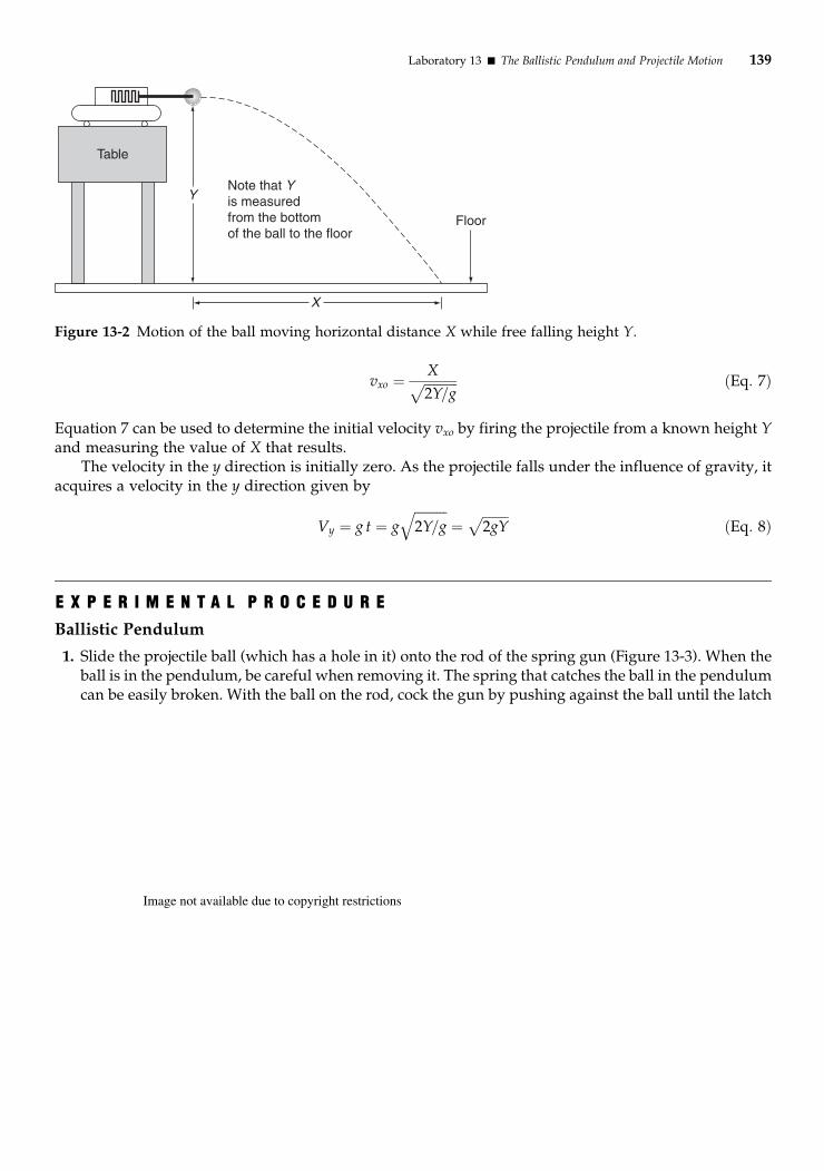
vxo ¼ Xffiffiffiffiffiffiffiffiffiffi2Y=g
p ðEq: 7Þ
Equation 7 can be used to determine the initial velocity vxo by firing the projectile from a known height Yand measuring the value of X that results.
The velocity in the y direction is initially zero. As the projectile falls under the influence of gravity, itacquires a velocity in the y direction given by
Vy ¼ g t ¼ gffiffiffiffiffiffiffiffiffiffi2Y=g
q¼
ffiffiffiffiffiffiffiffi2gY
pðEq: 8Þ
E X P E R I M E N T A L P R O C E D U R EBallistic Pendulum
1. Slide the projectile ball (which has a hole in it) onto the rod of the spring gun (Figure 13-3). When theball is in the pendulum, be careful when removing it. The spring that catches the ball in the pendulumcan be easily broken. With the ball on the rod, cock the gun by pushing against the ball until the latch
YNote that Yis measuredfrom the bottomof the ball to the floor
Floor
X
Table
Figure 13-2 Motion of the ball moving horizontal distance X while free falling height Y.
Laboratory 13 n The Ballistic Pendulum and Projectile Motion 139
Image not available due to copyright restrictions
catches. Be very careful not to get your hand caught in the spring gun mechanism. Fire the gun several timesto see how it operates. There are two common problems. If the ball does not catch in the pendulumbob, the spring in the bob should be adjusted or replaced. If the pawl that is designed to catch on thenotched track does not engage, the pendulum suspension should be adjusted by means of the screwsat the suspension points.
2. A sharp curved point on the side of the pendulum (or on somemodels a dot) marks the center of massof the pendulum-ball system. Let the pendulum bob hang vertically and measure the distance y1, thecenter of mass point above the base of the gun (Figure 13-1). Record the value of y1 in Data Table 1.
3. Fire the ball into the stationary pendulumwhile it hangs freely at rest. The pendulumwill catch the ball,swing up, and then lodge in the notched track. Record in Data Table 1 the position number, p, at whichthe pawl on the pendulum catches on the track. Measure the distance y2 of the center of mass pointabove the base of the apparatus (Figure 13-1) and record it in Data Table 1. Repeat this procedure fourmore times for a total of five trials, recording the position p andmeasuring the distance y2 for each trial.
4. Loosen the screws holding the pendulum in its support and remove the pendulum consisting of therod and the bob. Determine the mass of the pendulum (bob and rod) using a laboratory balance.Record the pendulum mass as M in Data Table 1. Determine the projectile ball mass and record it inData Table 1 as m.
Projectile Motion
In the following procedure, be extremely careful not to fire the ball when anyone is in a position to be struck by theball. Serious injury could result.
1. Raise the pendulum and secure it so that the ball can be fired under it.
2. Place the apparatus near the front edge of the laboratory table so that the ball will strike the floorbefore it strikes a wall or any other object. The gun must be fired each time from the same positionrelative to the table. It may be necessary to clamp the apparatus to the table. Place a piece of heavycardboard or some other object in a position to catch the ball after it strikes the floor but before itstrikes a wall. Do not allow the ball to strike a wall because it will likely damage it.Make several test firingsto locate the approximate place where the ball will land on the floor.
3. Place a sheet of white paper on the floor approximately centered where test firings have landed. Placea piece of carbon paper over the white paper so that the ball striking the carbon paper will leave a doton the white paper. Tape both of the papers to the floor.
4. Place the ball on the rod of the spring gun. The vertical distance Y that the ball will fall is the distancefrom the bottom of the ball to the floor as shown in Figure 13-2. Measure this distance to the nearest0.1 mm and record it in Data Table 2 as Y.
5. Fire the ball five times onto the same sheet of paper. Place the ball on the rod and measure thehorizontal distance X to the nearest 0.1mm from the center of the ball to the center of each dot onthe paper. Record these five values of X in Data Table 2.
C A L C U L A T I O N SBallistic Pendulum
1. Calculate the distance y2� y1 that the ball plus pendulum rises for each trial. Record these values andall other calculations in this section in Calculations Table 1.
2. From Equation 3 calculate the velocity V for each of the five trials.
3. From Equation 4 calculate the initial speed vxo for the five trials.
4. Calculate the mean vxo and the standard error av of the five values of vxo.
140 Physics Laboratory Manual n Loyd

Projectile Motion
1. Use Equation 7 to calculate the value of vxo for each of the five values ofX. Use a value of g¼ 9.80m/s2.Record these values in Calculations Table 2.
2. Calculate the mean vxo and the standard error av of the five values of vxo. Record them in CalculationsTable 2.
COPYRIG
HTª
2008ThomsonBrooks/Cole
Laboratory 13 n The Ballistic Pendulum and Projectile Motion 141

This page intentionally left blank

Name . . . . . . . . . . . . . . . . . . . . . . . . . . . . . . . . . . . . . . . . . . . . . . . . . . . . . . . . . . . . . . . . . . . . . . . . . Section . . . . . . . . . . . . . . . . Date . . . . . . . . . . . . . . . .
13 L A B O R A T O R Y 1 3 The Ballistic Pendulum and Projectile Motion
P R E - L A B O R A T O R Y A S S I G N M E N T1. What are the conditions under which the total momentum of a system of particles is conserved?
2. What kind of collision conserves kinetic energy?
3. What kind of collision does not conserve kinetic energy? What kind of collision results in themaximum loss of kinetic energy?
4. A ball of mass 0.075 kg is fired horizontally into a ballistic pendulum as shown in Figure 13-1. Thependulum mass is 0.350 kg. The ball is caught in the pendulum, and the center of mass of the systemrises a vertical distance of 0.145m in the earth’s gravitational field. What was the original speed of theball? Assume that g¼ 9.80m/s2. Show your work.
COPYRIG
HTª
2008ThomsonBrooks/Cole
143
5. How much kinetic energy was lost in the collision of Question 4? Show your work.
6. A projectile is fired in the earth’s gravitational field with a horizontal velocity of v¼ 9.00m/s. How fardoes it go in the horizontal direction in 0.550 s? Show your work.
7. How far does the projectile of Question 6 fall in the vertical direction in 0.550 s? Show your work.
8. A projectile is launched in the horizontal direction. It travels 2.050m horizontally while it falls 0.450mvertically, and it then strikes the floor. How long is the projectile in the air? Show your work.
9. What was the original velocity of the projectile described in Question 8? Show your work.
144 Physics Laboratory Manual n Loyd

Name . . . . . . . . . . . . . . . . . . . . . . . . . . . . . . . . . . . . . . . . . . . . . . . . . . . . . . . . . . . . . . . . . . . . . . . . . Section . . . . . . . . . . . . . . . . Date . . . . . . . . . . . . . . . .
Lab Partners . . . . . . . . . . . . . . . . . . . . . . . . . . . . . . . . . . . . . . . . . . . . . . . . . . . . . . . . . . . . . . . . . . . . . . . . . . . . . . . . . . . . . . . . . . . . . . . . . . . . . . . . . . . . . . . . . . . .
13 L A B O R A T O R Y 1 3 The Ballistic Pendulum and Projectile Motion
L A B O R A T O R Y R E P O R T
COPYRIG
HTª
2008ThomsonBrooks/Cole
Data Table 1
Trial p y2 (m)
1
2
3
4
5
m¼ kg M¼ kg y1¼ m
Calculations Table 1
y2� y1 (m) V (m/s) vxo (m/s)
vxo ¼ m=s av¼ m/s
Data Table 2
Trial X (m)
1
2
3
4
5
Y¼ m
Calculations Table 2
vxo (m/s)
vxo ¼ m=s av¼ m/s
145
S A M P L E C A L C U L A T I O N S1. y2� y1¼
2. V ¼ ffiffiffiffiffiffiffiffiffiffiffiffiffiffiffiffiffiffiffiffiffi2gðy2�y1Þ
p ¼
3. (Ballistic pendulum) vxo ¼ mþM
m
� V
4. ðProjectilemotionÞ ¼ vxo ¼ Xffiffiffiffiffiffiffiffiffiffiffi2Y=g
p
Q U E S T I O N S1. Compare the two different values of vxo. Calculate the difference and the percentage difference
between them. State whether the twomeasurements agree within the combined standard errors of thetwo values of vxo.
2. Can you make any statement about the accuracy of the two values of vxo? Are either of these valuesmore precise than the other? State clearly the basis for your answer in each case.
3. Calculate the loss in kinetic energy when the ball collides with the pendulum as the differencebetween ½mv2xo (the kinetic energy before) and ½ (mþM)V2 (the kinetic energy immediately after thecollision).
4. What is the fractional loss in kinetic energy? Calculate by dividing the loss calculated in Question 3 bythe original kinetic energy.
146 Physics Laboratory Manual n Loyd

5. Calculate the ratioM/(mþM) for the values of m andM in Data Table 1. Compare this ratio with theratio calculated in Question 4. Express the fractional loss of kinetic energy in symbol form and useequations from the lab to show it should equal M/(mþM).
6. It was assumed that the ball fired as a projectile moved exactly in the horizontal direction. If it movedat some small angle y to the horizontal, the correct equation would be ð4:90X2=v2oÞtan2y�X tan yþðYþ 4:90X2=v2oÞ ¼ 0 with the initial velocity labeled vo. Use the value of vo from the ballistic pendulummeasurement and the measured X and Y in the equation and solve for the angle y. If the ball was firedat angle y to the horizontal it would account for the difference in the two measured values of vo. Theequation is a quadratic in tan y and Y is negative in the equation. Is the y you found small enough thatit is plausible that the projectile might deviate that much from horizontal?
COPYRIG
HTª
2008ThomsonBrooks/Cole
Laboratory 13 n The Ballistic Pendulum and Projectile Motion 147

This page intentionally left blank
Conservation of Momentumon the Air Track
O B J E C T I V E So Determine the total momentum of two gliders on an air track before and after they collide.
o Evaluate the extent to which the total momentum of the system before the collision is equal to thetotal momentum of the system after the collision.
E Q U I P M E N T L I S T. Air track, air blower, three gliders (two approximately equal in mass), rubber band puck launcher,meter stick (if air track does not have marked scale)
. Four laboratory timers, laboratory balance and calibrated masses, masking tape
T H E O R YThe momentum of a mass m moving with a velocity v is
p ¼ mv ðEq: 1Þ
Momentum is a vector quantity because it is the product of a scalar (m) with a vector (v). Forces exertedbetween particles of a system are called internal forces, and they cannot change the momentum of thesystem. The total momentum of the system can change only if external forces act on the system.
Momentum is conserved in a collision between two objects because the forces that the objects exert oneach other are internal to the system. If p1
i and p2i stand for the initial momenta of two particles, and p1
f
and p2f stand for their final momenta after the collision, then
p1i þ p2
i ¼ p1f þ p2
f ðEq: 2Þ
Equation 2 implies that each of the vector components of momentum is conserved. For the linear airtrack a collision is one-dimensional, and the vectors are specified by writing momenta to the right aspositive and momenta to the left as negative. Friction on the gliders of the air track will be an externalforce, and friction must be negligible if Equation 2 is to be valid in this laboratory.
We will determine the constant velocities of two gliders before the collision and after the collision.A velocity will be determined bymeasuring the elapsed time for the glider to travel some known distance.
Physics Laboratory Manual n Loyd L A B O R A T O R Y 14
COPYRIG
HTª
2008ThomsonBrooks/Cole
149
ª 2008 Thomson Brooks/Cole, a part of TheThomson Corporation.Thomson, the Star logo, and Brooks/Cole are trademarks used herein under license. ALL RIGHTSRESERVED.No part of this workcovered by the copyright hereonmay be reproduced or used in any form or by any meansçgraphic, electronic, ormechanical, including photocopying, recording, taping,web distribution, informationstorage and retrieval systems,or in any othermannerçwithout the written permission of the publisher.
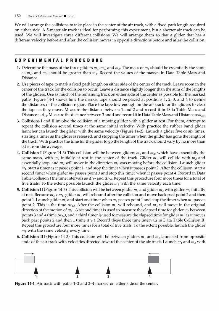
We will arrange the collisions to take place in the center of the air track, with a fixed path length requiredon either side. A 5-meter air track is ideal for performing this experiment, but a shorter air track can beused. We will investigate three different collisions. We will arrange them so that a glider that has adifferent velocity before and after the collision moves in opposite directions before and after the collision.
E X P E R I M E N T A L P R O C E D U R E1. Determine the mass of the three gliders m1, m2, andm3. The mass of m1 should be essentially the same
as m2, and m3 should be greater than m1. Record the values of the masses in Data Table Mass andDistance.
2. Use pieces of tape to mark a fixed path length on either side of the center of the track. Leave room in thecenter of the track for the collision to occur. Leave a distance slightly longer than the sum of the lengthsof the gliders. Use as much of the remaining track on either side of the center as possible for the markedpaths. Figure 14-1 shows how the marker tape should be placed at positions 1, 2, 3, and 4 to definethe distances of the collision region. Place the tape low enough on the air track for the gliders to clearthe tape as they move. Measure the distance between 1 and 2 and record it in Data Table Mass andDistanceasd12.Measure thedistancebetween3and4andrecord it inDataTableMassandDistanceasd34.
3. Collisions I and II involve the collision of a moving glider with a glider at rest. For them, attempt torepeat the collision several times at the same initial velocity. With practice the rubber band gliderlauncher can launch the glider with the same velocity (Figure 14-2). Launch a glider five or six times,starting a timer as the glider is released, and stopping the timer when the glider has gone the length ofthe track.With practice the time for the glider to go the length of the track should vary by nomore than0.1 s from the average.
4. Collision I (Figure 14-3) This collision will be between gliders m1 and m2, which have essentially thesame mass, with m2 initially at rest in the center of the track. Glider m1 will collide with m2 andessentially stop, and m2 will move in the direction m1 was moving before the collision. Launch gliderm1, start a timer as it passes point 1, and stop the timer when it passes point 2. After the collision, start asecond timer when glider m2 passes point 3 and stop this timer when it passes point 4. Record in DataTable Collision I the time intervals as Dt12 and Dt34. Repeat this procedure four more times for a total offive trials. To the extent possible launch the glider m1 with the same velocity each time.
5. Collision II (Figure 14-3) This collision will be between gliderm1 and gliderm3 with gliderm3 initiallyat rest. Becausem3 >m1, gliderm1 will rebound after the collision and move back past point 2 and thenpoint 1. Launch gliderm1 and start one timerwhenm1 passes point 1 and stop the timerwhenm1 passespoint 2. This is the time Dt12. After the collision m1 will rebound, and m3 will move in the originaldirection of themotion ofm1 . A second timer is used tomeasure the elapsed time for gliderm3 betweenpoints 3 and 4 (timeDt34), and a third timer is used tomeasure the elapsed time for gliderm1 as it movesback past points 2 and then 1 (time Dt21). Record these three time intervals in Data Table Collision II.Repeat this procedure four more times for a total of five trials. To the extent possible, launch the gliderm1 with the same velocity every time.
6. Collision III (Figure 14-3) This collision will be between gliders m1 and m3 launched from oppositeends of the air track with velocities directed toward the center of the air track. Launch m1 andm3 with
321 4
Figure 14-1 Air track with paths 1–2 and 3–4 marked on either side of the center.
150 Physics Laboratory Manual n Loyd
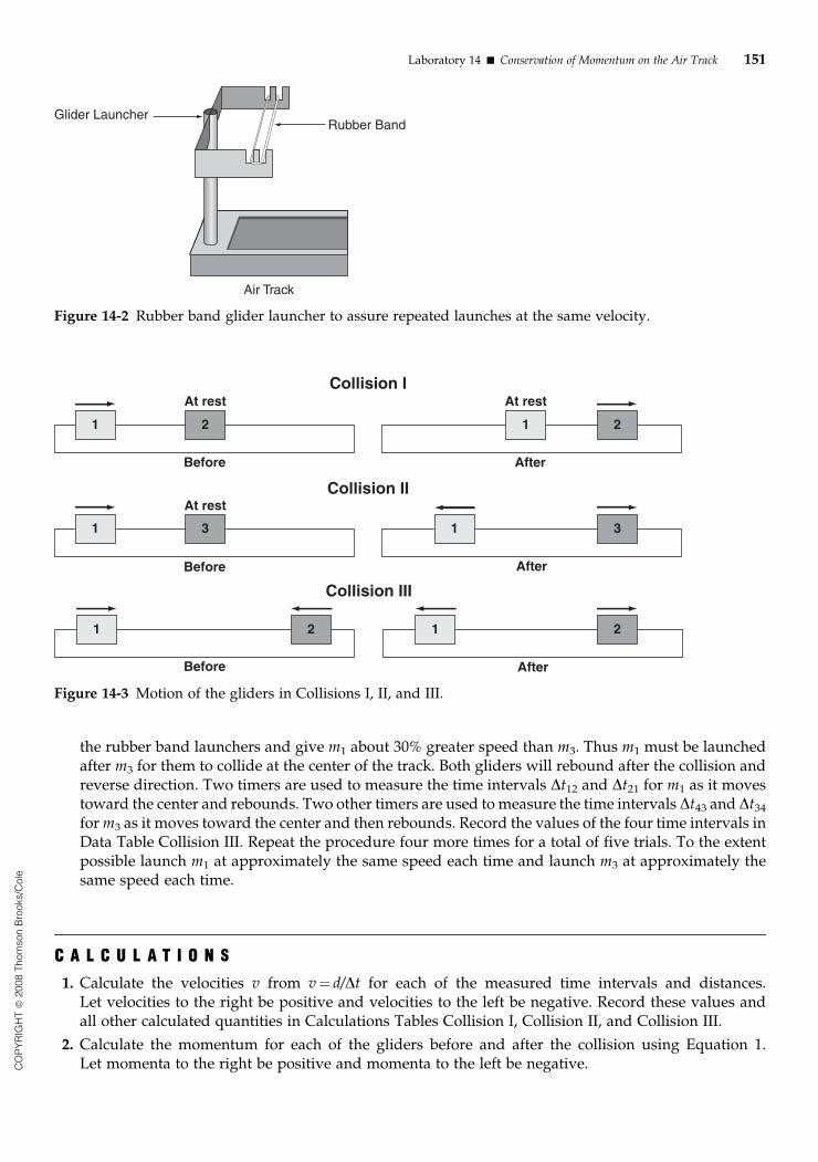
the rubber band launchers and give m1 about 30% greater speed than m3. Thus m1 must be launchedafter m3 for them to collide at the center of the track. Both gliders will rebound after the collision andreverse direction. Two timers are used to measure the time intervals Dt12 and Dt21 for m1 as it movestoward the center and rebounds. Two other timers are used to measure the time intervals Dt43 and Dt34form3 as it moves toward the center and then rebounds. Record the values of the four time intervals inData Table Collision III. Repeat the procedure four more times for a total of five trials. To the extentpossible launch m1 at approximately the same speed each time and launch m3 at approximately thesame speed each time.
C A L C U L A T I O N S1. Calculate the velocities v from v¼ d/Dt for each of the measured time intervals and distances.
Let velocities to the right be positive and velocities to the left be negative. Record these values andall other calculated quantities in Calculations Tables Collision I, Collision II, and Collision III.
2. Calculate the momentum for each of the gliders before and after the collision using Equation 1.Let momenta to the right be positive and momenta to the left be negative.C
OPYRIG
HTª
2008ThomsonBrooks/Cole
Glider Launcher
Air Track
Rubber Band
Figure 14-2 Rubber band glider launcher to assure repeated launches at the same velocity.
Collision I
Collision II
Collision III
Before After
Before After
At rest
At rest
Before
1
1
21 1 2
3 1 3
1 22
After
At rest
Figure 14-3 Motion of the gliders in Collisions I, II, and III.
Laboratory 14 n Conservation of Momentum on the Air Track 151

3. For Collision I compare the percentage difference of the momentum of the first glider before thecollision to the momentum of the second glider after the collision.
4. For Collisions II and III, calculate the total momentum of both gliders before and the total momentumof both gliders after the collision. Then calculate the percentage difference in the total momentumbefore the collision and the total momentum after the collision.
(Instead of using hand timers the laboratory can be done with photogates to more accurately measure the timeintervals with the appropriate changes in procedures.)
152 Physics Laboratory Manual n Loyd

Name . . . . . . . . . . . . . . . . . . . . . . . . . . . . . . . . . . . . . . . . . . . . . . . . . . . . . . . . . . . . . . . . . . . . . . . . . Section . . . . . . . . . . . . . . . . Date . . . . . . . . . . . . . . . .
14 L A B O R A T O R Y 1 4 Conservation of Momentum on the Air Track
P R E - L A B O R A T O R Y A S S I G N M E N T1. What is the definition of momentum?
2. What conditions must be satisfied for momentum to be conserved?
3. Two pieces of tape are placed a distance 1.50 m apart on an air track. A 0.350 kg glider on the airtrack takes time Dt¼ 1.30 s to move between the two pieces of tape. What is the velocity of the glider?What is its momentum? Show your work.
4. A glider of massm1¼ 0.350 kgmoves with a velocity of 0.850m/s to the right on an air track. It collideswith a glider of mass m2¼ 0.350 kg at rest. Glider m1 stops, and m2 moves in the direction that m1 wastraveling. What is the velocity of m2? Show your work.
COPYRIG
HTª
2008ThomsonBrooks/Cole
153

5. An air track glider of massm1¼ 0.200 kgmoving at 0.750 m/s to the right collides with a glider of massm2¼ 0.400 kg at rest. Ifm1 rebounds and moves to the left with a speed of 0.250 m/s, what is the speedand direction of m2 after the collision? (Hint—Momentum is a vector quantity, and direction isindicated by the sign of the momentum.) Show your work.
6. For the collision in Question 5, calculate the original kinetic energy of the system before the collision.Calculate the total kinetic energy after the collision. What happened to the lost energy? Showyour work.
7. An air track glider of mass m1¼ 0.300 kg moving at a speed of 0.800 m/s to the right collides with aglider of mass m2¼ 0.300 kg moving at a speed of 0.400 m/s in the opposite direction. After thecollisionm1 rebounds at speed 0.200 m/s to the left. After the collision, what is the speed and directionof m2? Show your work.
154 Physics Laboratory Manual n Loyd

Name . . . . . . . . . . . . . . . . . . . . . . . . . . . . . . . . . . . . . . . . . . . . . . . . . . . . . . . . . . . . . . . . . . . . . . . . . Section . . . . . . . . . . . . . . . . Date . . . . . . . . . . . . . . . .
Lab Partners . . . . . . . . . . . . . . . . . . . . . . . . . . . . . . . . . . . . . . . . . . . . . . . . . . . . . . . . . . . . . . . . . . . . . . . . . . . . . . . . . . . . . . . . . . . . . . . . . . . . . . . . . . . . . . . . . . . .
14 L A B O R A T O R Y 1 4 Conservation of Momentum on the Air Track
L A B O R A T O R Y R E P O R T
COPYRIG
HTª
2008ThomsonBrooks/Cole
Data Table Mass and Distance
m1 (kg) m2 (kg) m3 (kg) d12 (m) d34 (m)
Data Table Collision I
Trial 1 Trial 2 Trial 3 Trial 4 Trial 5
m1 Before Dt12 (s)
m2 After Dt34 (s)
Calculations Table Collision I
Trial 1 Trial 2 Trial 3 Trial 4 Trial 5
m1 Before v1 (m/s)
p1 (kg�m/s)
m2 After v2 (m/s)
p2 (kg�m/s)
% Difference p1 and p2
155

Data Table Collision II
Trial 1 Trial 2 Trial 3 Trial 4 Trial 5
m1 Before Dt12 (s)
m1 After Dt21 (s)
m2 After Dt34 (s)
Calculations Table Collision II
Trial 1 Trial 2 Trial 3 Trial 4 Trial 5
m1 Before v1i ðm=sÞ
p1iðkg�m=sÞ
m1 After v1f ðm=sÞ
p1fðkg�m=sÞ
m3 After v3f ðm=sÞ
p3fðkg�m=sÞ
After ¼ p1f þ p3
f ¼
% Diff
Data Table Collision III
Trial 1 Trial 2 Trial 3 Trial 4 Trial 5
m1 Before Dt12 (s)
m3 Before Dt43 (s)
m1 After Dt21 (s)
m3 After Dt34 (s)
156 Physics Laboratory Manual n Loyd

S A M P L E C A L C U L A T I O N S1. v1¼ d12/Dt12¼2. p1¼ (m1)(v1)¼3. Total p ðbeforeÞ ¼ p1
i þ p3i ¼
4. % Difference¼5. Ki ¼ ½m1ðv1iÞ2 þ½m2ðv2iÞ2 ¼6. DK¼Kf�Ki¼7. % Lost¼DK/Ki� 100%¼
Q U E S T I O N S1. Consider the percentage differences between the total momentum before the collision and the total
momentum after the collision for the various trials of Collisions I, II, and III. If they are less than 10%they are good evidence that momentum is conserved, and if they are less than 5% they are very goodevidence. To what extent do your data indicate that momentum is conserved?
COPYRIG
HTª
2008ThomsonBrooks/Cole
Calculations Table Collision III
Trial 1 Trial 2 Trial 3 Trial 4 Trial 5
m1 Before v1i ðm=sÞ
p1iðkg�m=sÞ
m3 Before v3i ðm=sÞ
P3iðkg�m=sÞ
m1 After v1f ðm=sÞ
p1fðkg�m=sÞ
m3 After v3f ðm=sÞ
p3fðkg�m=sÞ
p1i þ p3
i ¼
p1f þ p3
f ¼
% Diff
Laboratory 14 n Conservation of Momentum on the Air Track 157

2. For each of the Collisions I, II, and III, consider the one trial that has the smallest percentage differenceand calculate Ki, Kf, DK, and the % Lost for that trial. What happens to the lost energy?
Collision I Trial Ki ¼ Kf ¼ DK ¼ %Lost ¼Collision II Trial Ki ¼ Kf ¼ DK ¼ %Lost ¼Collision III Trial Ki ¼ Kf ¼ DK ¼ %Lost ¼
3. Is the kinetic energy approximately conserved for any of the collisions that you calculated? If so, statewhich one or ones and give your evidence.
158 Physics Laboratory Manual n Loyd

Conservation of Momentumon the Air Table
O B J E C T I V E So Determine the velocities and momenta of pucks on an air table before and after several different
two-dimensional collisions.
o Impose a coordinate system on each collision to resolve the momenta into components andevaluate the extent to which momentum is conserved for each component.
E Q U I P M E N T L I S T. Air table with pucks, sparktimer, air pump, foot switch, lead weights, Velcro collars, and level
. Carbon paper, recording paper, meter stick or ruler, protractor, and square
T H E O R YThe momentum of an object of mass m moving with a velocity v is
p ¼ mv ðEq: 1Þ
Momentum is a vector quantity because it is the product of a scalar (m) with a vector (v). For a system ofparticles the total momentum of the system is constant if there are no external forces acting on the system.The forces exerted between particles of the system are called internal forces, and they cannot change themomentum of the system.
Momentum is conserved in collisions between two objects because the forces that the objects exert oneach other are internal to the system. If p1
i and p2i are the initial momenta of two particles, and p1
f and p2f
are their final momenta after the collision, then
p1i þ p2
i ¼ p1f þ p2
f ðEq: 2Þ
A collision where particles stick together is called a completely inelastic collision. Such a collision willresult in the maximum possible loss of kinetic energy.
Physics Laboratory Manual n Loyd L A B O R A T O R Y 15
COPYRIG
HTª
2008ThomsonBrooks/Cole
159
ª 2008 Thomson Brooks/Cole, a part of TheThomson Corporation.Thomson, the Star logo, and Brooks/Cole are trademarks used herein under license. ALL RIGHTSRESERVED.No part of this workcovered by the copyright hereonmay be reproduced or used in any form or by any meansçgraphic, electronic, ormechanical, including photocopying, recording, taping,web distribution, informationstorage and retrieval systems,or in any othermannerçwithout the written permission of the publisher.

Figure 15-1 shows amassm1 with velocity v1 and amassm2 with velocity v2 that collide at the origin ofa coordinate system. After the collision they have velocities v3 and v4. For that collision with coordinates asshown, the equations that represent the conservation of momentum are
x direction m1v1cos y1 þm2v2cos y2 ¼ m2v4cos y4 þm1v3cos y3 ðEq: 3Þ
y direction m1v1sin y1 þm2v2sin y2 ¼ m1v3sin y3 þm2v4sin y4 ðEq: 4Þ
Wewill use collisions on the air table to investigate this general case and several simpler special cases.Simplified collisions occur when m1¼m2, when one of the masses is originally at rest, and when thecollision is head-on with all motion along a single line.
E X P E R I M E N T A L P R O C E D U R E1. Unless you have prior experience with the air table (Figure 15-2) read the instruction manual for the
air table to become familiar with its operation including the air pump, sparktimer, and foot switch. Becareful not to touch the pucks except by the insulated tubes when the sparktimer is in operation.
2. Level the air table with the three adjustable legs until a puck placed near the center of the table isessentially motionless. It is especially critical to have the table as level as possible for these collision eventsbecause several of the collisions are to be made with one of the pucks initially at rest.
3. Set the sparktimer to 20.0Hz. Perform each of the four collisions described below. Start the sparktimerafter the pucks are launched, and stop it before the pucks collide with the edge of the table. Frictionwill cause the experimental results to disagree with the theory, and the effect is larger for low speeds.For best results the pucks should move as fast as reasonable. However, it is possible to damage theglass tops of the tables if the pucks are thrown too fast. Be very careful not to damage the air table. Consultyour instructor for advice about the speed of the pucks. Use the same sheet of carbon paper for allmeasurements, but use a new sheet of recording paper for each collision.
4. Collision I Use a laboratory balance to determine the mass of two pucks that are approximately thesame mass and record in the Data Table. Label one puck #1 and the other #2. Launch puck 1 from nearone corner so that it strikes puck 2, which is at rest near the center of the table. The collision shouldnot be head-on. The pucks should move at a large angle relative to each other after the collision.
v2 (before)v4 (after)
v3 (after)
m1 (after)
m2 (after)
m1 (before)
m2 (before)
�xv1 (before)
�1
�2
�3
�4
Figure 15-1 Collision between mass m1 and m2, both with an initial velocity.
160 Physics Laboratory Manual n Loyd
Before removing the recording paper, label each sparktimer track with the puck number and thedirection that each puckmoved before and after the collision. Label each collision before removing therecording paper from the table. Label this recording as Collision I, and set it aside for future analysis.
5. Collision II Use the same pucks as Collision I, but launch them both at the same time from adjacentcorners of the table so they collide at the center at an angle of about 908. Label the tracks in the mannerdescribed above. Label it as Collision II, and set it aside for future analysis.
6. Collision III Use the same procedure as Collision II but use masses that are not equal. Use puck 1 asit is. Place several of the lead weights that fit over the pucks to increase the mass of puck 2. Determinethe mass of puck 2 with the lead on it, and record the results in the Data Table. Launch the pucks fromadjacent corners so they collide near the center. Label the tracks and recording paper as above, and setthe paper aside for future analysis.
7. Collision IV Remove the lead from puck 2. Place Velcro collars on each of the pucks. Determine themass of each puck, and record it in the Data Table. With Velcro collars the pucks will stick together,and the collision will be completely inelastic. Launch the two pucks of approximately equal mass fromadjacent corners of the table so they collide near the center. It might be necessary to try this severaltimes. When the pucks stick together they might have a tendency to rotate about a common center ofmass as they move together. Instead, it is necessary that after the collision the trace shows thecombined pucks making parallel tracks as they move together. That is evidence that no rotation isoccurring. It may take several traces to achieve parallel tracks. Label the acceptable recording, and setit aside for future analysis.
8. For each collision determine the displacement Ds along the four tracks that represent the motion of thepucks before and after the collision. Measure the Ds of the puck for four spark intervals or Dt¼ 0.200 s.Be sure that the appropriate Ds is associated with each of the pucks both before and after the collision.Record all displacements Ds in the Data Tables.
9. For each of the collisions draw an x coordinate axis on the recording paper. This is an arbitrary choice,but it will save work to choose the þx direction to be the direction of the initial motion of one of thepucks. That puck would then initially have only an x component, with y component zero. Determinethe components for the other puck before the collision, and for both the pucks after the collision, byfinding the angle their tracks make with the þx axis. This process is illustrated in Figure 15-3. The þxaxis has been chosen to be in the direction of the initial motion of puck 1. The other angles are thendetermined by the angle each puck’s motion makes with the þx axis. The x components are given bythe cosine and the y components by the sine.
For each of the four collisions draw theþx axis through the points of the initial motion of puck 1 in thedirection of its motion. Using a protractor, carefully measure the angle of the other three tracks with theC
OPYRIG
HTª
2008ThomsonBrooks/Cole
Laboratory 15 n Conservation of Momentum on the Air Table 161
Image not available due to copyright restrictions
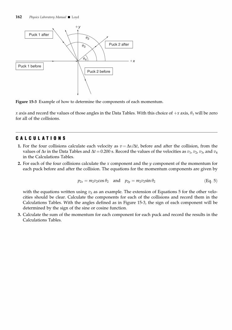
x axis and record the values of those angles in the Data Tables. With this choice of þx axis, y1 will be zerofor all of the collisions.
C A L C U L A T I O N S1. For the four collisions calculate each velocity as v¼Ds/Dt, before and after the collision, from the
values of Ds in the Data Tables and Dt¼ 0.200 s. Record the values of the velocities as v1, v2, v3, and v4in the Calculations Tables.
2. For each of the four collisions calculate the x component and the y component of the momentum foreach puck before and after the collision. The equations for the momentum components are given by
p2x ¼ m2v2cos y2 and p2y ¼ m2v2sin y2 ðEq: 5Þ
with the equations written using v2 as an example. The extension of Equations 5 for the other velo-cities should be clear. Calculate the components for each of the collisions and record them in theCalculations Tables. With the angles defined as in Figure 15-3, the sign of each component will bedetermined by the sign of the sine or cosine function.
3. Calculate the sum of the momentum for each component for each puck and record the results in theCalculations Tables.
�y
�x�4
�3
�2
Puck 2 beforePuck 1 before
Puck 2 after
Puck 1 after
Figure 15-3 Example of how to determine the components of each momentum.
162 Physics Laboratory Manual n Loyd
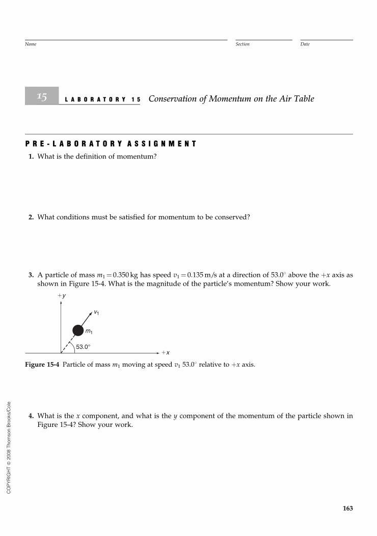
Name . . . . . . . . . . . . . . . . . . . . . . . . . . . . . . . . . . . . . . . . . . . . . . . . . . . . . . . . . . . . . . . . . . . . . . . . . Section . . . . . . . . . . . . . . . . Date . . . . . . . . . . . . . . . .
15 L A B O R A T O R Y 1 5 Conservation of Momentum on the Air Table
P R E - L A B O R A T O R Y A S S I G N M E N T1. What is the definition of momentum?
2. What conditions must be satisfied for momentum to be conserved?
3. A particle of mass m1¼ 0.350 kg has speed v1¼ 0.135m/s at a direction of 53.08 above the þx axis asshown in Figure 15-4. What is the magnitude of the particle’s momentum? Show your work.
4. What is the x component, and what is the y component of the momentum of the particle shown inFigure 15-4? Show your work.
COPYRIG
HTª
2008ThomsonBrooks/Cole
�y
v1
m1
53.0°�x
Figure 15-4 Particle of mass m1 moving at speed v1 53.08 relative to þx axis.
163
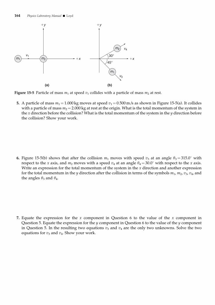
5. A particle of mass m1¼ 1.000 kg moves at speed v1¼ 0.500m/s as shown in Figure 15-5(a). It collideswith a particle of massm2¼ 2.000 kg at rest at the origin. What is the total momentum of the system inthe x direction before the collision?What is the total momentum of the system in the y direction beforethe collision? Show your work.
6. Figure 15-5(b) shows that after the collision m1 moves with speed v3 at an angle y3¼ 315.08 withrespect to the x axis, and m2 moves with a speed v4 at an angle y4¼ 30.08 with respect to the x axis.Write an expression for the total momentum of the system in the x direction and another expressionfor the total momentum in the y direction after the collision in terms of the symbols m1, m2, v3, v4, andthe angles y3 and y4.
7. Equate the expression for the x component in Question 6 to the value of the x component inQuestion 5. Equate the expression for the y component in Question 6 to the value of the y componentin Question 5. In the resulting two equations v3 and v4 are the only two unknowns. Solve the twoequations for v3 and v4. Show your work.
�x
�y
m1 m2
v1�x
�y
m2
m1
v4
v3
30°
45°
(a) (b)
Figure 15-5 Particle of mass m1 at speed v1 collides with a particle of mass m2 at rest.
164 Physics Laboratory Manual n Loyd

Name . . . . . . . . . . . . . . . . . . . . . . . . . . . . . . . . . . . . . . . . . . . . . . . . . . . . . . . . . . . . . . . . . . . . . . . . . Section . . . . . . . . . . . . . . . . Date . . . . . . . . . . . . . . . .
Lab Partners . . . . . . . . . . . . . . . . . . . . . . . . . . . . . . . . . . . . . . . . . . . . . . . . . . . . . . . . . . . . . . . . . . . . . . . . . . . . . . . . . . . . . . . . . . . . . . . . . . . . . . . . . . . . . . . . . . . .
15 L A B O R A T O R Y 1 5 Conservation of Momentum on the Air Table
L A B O R A T O R Y R E P O R T(Record all masses in kg, all displacements in m, all velocities inm/s, and all momenta in kg-m/s.)
COPYRIG
HTª
2008ThomsonBrooks/Cole
Data Table Collision I
m1 m2 Ds1 Ds2 Ds3 Ds4 y1 y2 y3 y4
Calculations Table Collision I
v1 v2 p1x p1y p2x p2y p1xþ p2x p1yþ p2y
v3 v4 p3x p3y p4x p4y p3xþ p4x p3yþ p4y
Data Table Collision II
m1 m2 Ds1 Ds2 Ds3 Ds4 y1 y2 y3 y4
Calculations Table Collision II
v1 v2 p1x p1y p2x p2y p1xþ p2x p1yþ p2y
v3 v4 p3x p3y p4x p4y p3xþ p4x p3yþ p4y
165

S A M P L E C A L C U L A T I O N S1. vi¼Dsi/D t¼2. pi¼mi vi¼3. pix¼ pi cos yi¼4. piy¼ pi sin yi¼5. %Diff x ¼ ððp3x þ p4xÞ�ðp1x þ p2xÞÞ=ð½ðp1x þ p2x þ p3x þ p4xÞÞ � 100% ¼
6. p1ðinitialÞ ¼ffiffiffiffiffiffiffiffiffiffiffiffiffiffiffiffiffiffiffiffiffiffiffiffiffiffiffiffiffiffiffiffiffiffiffiffiffiffiffiffiffiffiffiffiffiffiffiffiffiffiffiffiffiðp1x þ p2xÞ2 þ ðp1y þ p2yÞ2
q¼
7. %Diff= pðinitialÞ ¼ ððp3x þ p4xÞ�ðp1x þ p2xÞÞ=ðpðinitialÞÞ � 100% ¼8. K¼½mv2¼9. DK¼Kf�Ki ¼10. %LossK¼DK/K� 100%¼
Data Table Collision III
m1 m2 Ds1 Ds2 Ds3 Ds4 y1 y2 y3 y4
Calculations Table Collision III
v1 v2 p1x p1y p2x p2y p1xþ p2x p1yþ p2y
v3 v4 p3x p3y p4x p4y p3xþ p4x p3yþ p4y
Calculations Table Collision IV
v1 v2 p1x p1y p2x p2y p1xþ p2x p1yþ p2y
v3 v4 p3x p3y p4x p4y p3xþ p4x p3yþ p4y
Data Table Collision IV
m1 m2 Ds1 Ds2 Ds3 Ds4 y1 y2 y3 y4
166 Physics Laboratory Manual n Loyd
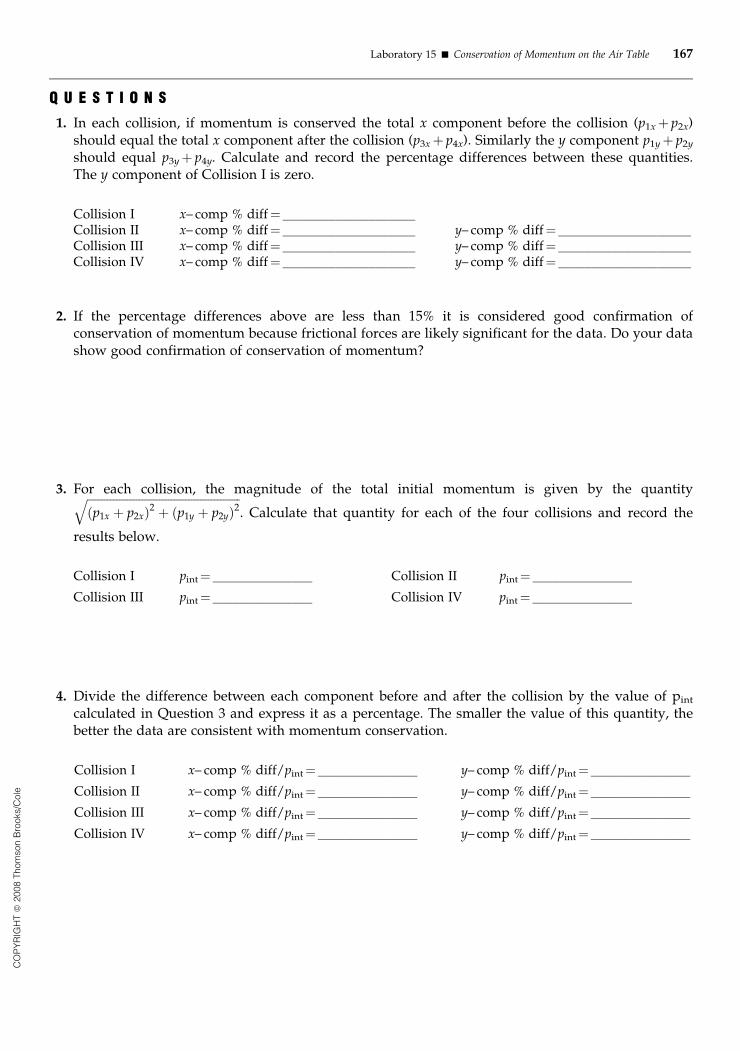
Q U E S T I O N S1. In each collision, if momentum is conserved the total x component before the collision (p1xþ p2x)
should equal the total x component after the collision (p3xþ p4x). Similarly the y component p1yþ p2yshould equal p3yþ p4y. Calculate and record the percentage differences between these quantities.The y component of Collision I is zero.
2. If the percentage differences above are less than 15% it is considered good confirmation ofconservation of momentum because frictional forces are likely significant for the data. Do your datashow good confirmation of conservation of momentum?
3. For each collision, the magnitude of the total initial momentum is given by the quantityffiffiffiffiffiffiffiffiffiffiffiffiffiffiffiffiffiffiffiffiffiffiffiffiffiffiffiffiffiffiffiffiffiffiffiffiffiffiffiffiffiffiffiffiffiffiffiffiffiffiffiffiffiðp1x þ p2xÞ2 þ ðp1y þ p2yÞ2
q. Calculate that quantity for each of the four collisions and record the
results below.
4. Divide the difference between each component before and after the collision by the value of pint
calculated in Question 3 and express it as a percentage. The smaller the value of this quantity, thebetter the data are consistent with momentum conservation.
COPYRIG
HTª
2008ThomsonBrooks/Cole
Collision I x– comp % diff¼ ____________________Collision II x– comp % diff¼ ____________________ y– comp % diff¼ ____________________Collision III x– comp % diff¼ ____________________ y– comp % diff¼ ____________________Collision IV x– comp % diff¼ ____________________ y– comp % diff¼ ____________________
Collision I pint¼ _______________ Collision II pint¼ _______________
Collision III pint¼ _______________ Collision IV pint¼ _______________
Collision I x– comp % diff/pint¼ _______________ y– comp % diff/pint¼ _______________
Collision II x– comp % diff/pint¼ _______________ y– comp % diff/pint¼ _______________
Collision III x– comp % diff/pint¼ _______________ y– comp % diff/pint¼ _______________
Collision IV x– comp % diff/pint¼ _______________ y– comp % diff/pint¼ _______________
Laboratory 15 n Conservation of Momentum on the Air Table 167

This page intentionally left blank

Centripetal Accelerationof an Object in CircularMotion
O B J E C T I V E So Investigate how the period T of an object that rotates in a circle is related to themass of the objectM,
speed v, and radius R of the circle.
o Determine the centripetal force F as the force required to stretch a spring.
E Q U I P M E N T L I S T. Hand-operated centripetal force apparatus (The device described is available from Sargent-WelchScientific Company.)
. Laboratory balance, calibrated slotted masses, mass holder, laboratory timer, and metal ruler
T H E O R YAn object moving in a circle at constant speed has a velocity vector that is always tangent to the circle.The direction of the velocity is continuously changing. The object is accelerated because acceleration isby definition a change in velocity per unit time. Figure 16-1 shows the velocity vector at points around thecircle for an object moving in a circle at constant speed. The lengths of the vectors are the same becausethe speed is constant, and the direction of the vectors indicates the direction of the velocity at that point.Also shown in Figure 16-1 are the velocity vectors vi and vf at two times ti and tf. In the third part of thefigure is the vector difference Dv¼ vf� vi indicating that the change in velocity Dv always points towardthe center of the circle. The acceleration a is
a ¼ Dv=Dt ðEq: 1Þ
The acceleration a is in the direction of Dv. It points toward the center of the circle and has magnitude
a ¼ v2=R ðEq: 2Þ
Physics Laboratory Manual n Loyd L A B O R A T O R Y 16
COPYRIG
HTª
2008ThomsonBrooks/Cole
169
ª 2008 Thomson Brooks/Cole, a part of TheThomson Corporation.Thomson, the Star logo, and Brooks/Cole are trademarks used herein under license. ALL RIGHTSRESERVED.No part of this workcovered by the copyright hereonmay be reproduced or used in any form or by any meansçgraphic, electronic, ormechanical, including photocopying, recording, taping,web distribution, informationstorage and retrieval systems,or in any othermannerçwithout the written permission of the publisher.
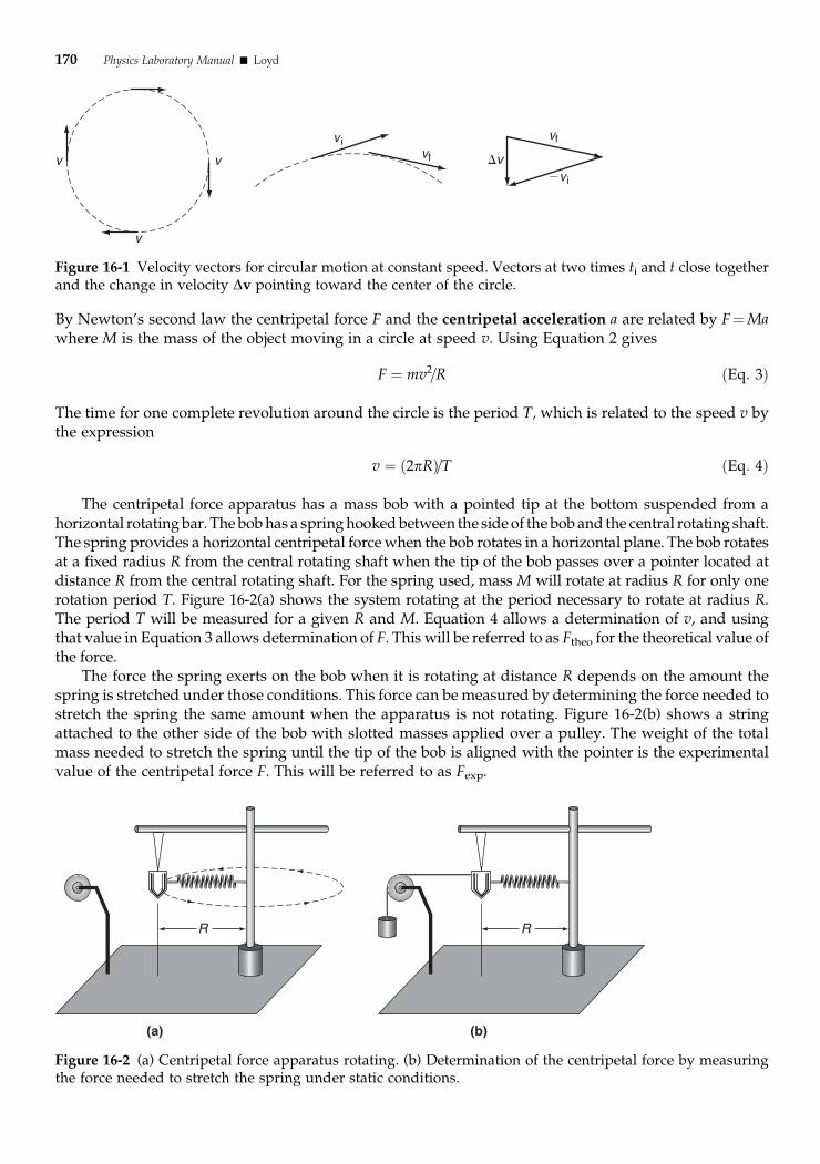
By Newton’s second law the centripetal force F and the centripetal acceleration a are related by F¼Mawhere M is the mass of the object moving in a circle at speed v. Using Equation 2 gives
F ¼ mv2=R ðEq: 3Þ
The time for one complete revolution around the circle is the period T, which is related to the speed v bythe expression
v ¼ ð2pRÞ=T ðEq: 4Þ
The centripetal force apparatus has a mass bob with a pointed tip at the bottom suspended from ahorizontal rotatingbar. Thebobhasa springhookedbetween the side of theboband the central rotating shaft.The spring provides a horizontal centripetal forcewhen the bob rotates in a horizontal plane. The bob rotatesat a fixed radius R from the central rotating shaft when the tip of the bob passes over a pointer located atdistance R from the central rotating shaft. For the spring used, mass M will rotate at radius R for only onerotation period T. Figure 16-2(a) shows the system rotating at the period necessary to rotate at radius R.The period T will be measured for a given R and M. Equation 4 allows a determination of v, and usingthat value in Equation 3 allows determination of F. This will be referred to as Ftheo for the theoretical value ofthe force.
The force the spring exerts on the bob when it is rotating at distance R depends on the amount thespring is stretched under those conditions. This force can be measured by determining the force needed tostretch the spring the same amount when the apparatus is not rotating. Figure 16-2(b) shows a stringattached to the other side of the bob with slotted masses applied over a pulley. The weight of the totalmass needed to stretch the spring until the tip of the bob is aligned with the pointer is the experimentalvalue of the centripetal force F. This will be referred to as Fexp.
v v
v ivf
vf
�v i
�v
v
Figure 16-1 Velocity vectors for circular motion at constant speed. Vectors at two times ti and t close togetherand the change in velocity Dv pointing toward the center of the circle.
R
(a)
R
(b)
Figure 16-2 (a) Centripetal force apparatus rotating. (b) Determination of the centripetal force by measuringthe force needed to stretch the spring under static conditions.
170 Physics Laboratory Manual n Loyd
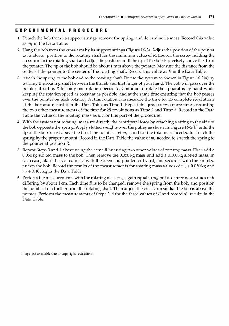
E X P E R I M E N T A L P R O C E D U R E1. Detach the bob from its support strings, remove the spring, and determine its mass. Record this value
as mb in the Data Table.
2. Hang the bob from the cross arm by its support strings (Figure 16-3). Adjust the position of the pointerto its closest position to the rotating shaft for the minimum value of R. Loosen the screw holding thecross arm in the rotating shaft and adjust its position until the tip of the bob is precisely above the tip ofthe pointer. The tip of the bob should be about 1 mm above the pointer. Measure the distance from thecenter of the pointer to the center of the rotating shaft. Record this value as R in the Data Table.
3. Attach the spring to the bob and to the rotating shaft. Rotate the system as shown in Figure 16-2(a) bytwirling the rotating shaft between the thumb and first finger of your hand. The bob will pass over thepointer at radius R for only one rotation period T. Continue to rotate the apparatus by hand whilekeeping the rotation speed as constant as possible, and at the same time ensuring that the bob passesover the pointer on each rotation. At this rotation rate measure the time for 25 complete revolutionsof the bob and record it in the Data Table as Time 1. Repeat this process two more times, recordingthe two other measurements of the time for 25 revolutions as Time 2 and Time 3. Record in the DataTable the value of the rotating mass as mb for this part of the procedure.
4. With the system not rotating, measure directly the centripetal force by attaching a string to the side ofthe bob opposite the spring. Apply slotted weights over the pulley as shown in Figure 16-2(b) until thetip of the bob is just above the tip of the pointer. Let ma stand for the total mass needed to stretch thespring by the proper amount. Record in the Data Table the value of ma needed to stretch the spring tothe pointer at position R.
5. Repeat Steps 3 and 4 above using the same R but using two other values of rotating mass. First, add a0.050 kg slotted mass to the bob. Then remove the 0.050 kg mass and add a 0.100 kg slotted mass. Ineach case, place the slotted mass with the open end pointed outward, and secure it with the knurlednut on the bob. Record the results of the measurements for rotating mass values of mbþ 0.050 kg andmbþ 0.100 kg in the Data Table.
6. Perform themeasurements with the rotatingmassmrot again equal tomb, but use three new values ofRdiffering by about 1 cm. Each time R is to be changed, remove the spring from the bob, and positionthe pointer 1 cm further from the rotating shaft. Then adjust the cross arm so that the bob is above thepointer. Perform the measurements of Steps 2–4 for the three values of R and record all results in theData Table.
Laboratory 16 n Centripetal Acceleration of an Object in Circular Motion 171
Image not available due to copyright restrictions

C A L C U L A T I O N S1. Calculate the mean of the three trials of the time for 25 complete revolutions, and record it in the
Calculations Table as Time. Divide the value of Time by 25, and record the result in the CalculationsTable as the period T.
2. Use Equation 4 to calculate v from the measured values of R and T, and record the results in theCalculations Table.
3. Use Equation 3 to calculate the theoretical value for the centripetal force from the values ofM, v, andR.Record the results in the Calculations Table as Ftheo.
4. Calculate the experimental value for the centripetal force as ma g from the values of ma. Use a value of9.80 m/s2 for g. Record the results in the Calculations Table as Fexp.
5. Calculate the percentage difference between the values of Ftheo and Fexp. Record the results in theCalculations Table.
172 Physics Laboratory Manual n Loyd
Name . . . . . . . . . . . . . . . . . . . . . . . . . . . . . . . . . . . . . . . . . . . . . . . . . . . . . . . . . . . . . . . . . . . . . . . . . Section . . . . . . . . . . . . . . . . Date . . . . . . . . . . . . . . . .
16 L A B O R A T O R Y 1 6 Centripetal Acceleration of an Object inCircular Motion
P R E - L A B O R A T O R Y A S S I G N M E N T1. If a particle moves in a circle of radius R at constant speed v its acceleration is (a) directed toward
the center of the circle (b) equal to v2/R (c) because the direction of the velocity vector changescontinuously (d) all of the above are true.
2. If a particle moves in a circle of radius R¼ 1.35m at a constant speed of v¼ 6.70 m/s, what is themagnitude and direction of its centripetal acceleration?
3. If the mass of the particle in Question 2 is 0.350 kg, what is the magnitude and direction of thecentripetal force on it? Show your work.
4. A 0.500 kg particle moves in a circle of radius R¼ 0.150m at constant speed. The time for 20 completerevolutions is 31.7 s. What is the period T of the motion? What is the speed of the particle? Show yourwork.
COPYRIG
HTª
2008ThomsonBrooks/Cole
173

5. What is the centripetal acceleration of the particle in Question 4? What is the centripetal force on theparticle? Show your work.
6. For the apparatus used in this laboratory the centripetal force is the same for a fixed radius R ofrotation. Why is that statement true for this apparatus? (Hint—What provides the centripetal force onthe rotating mass for this apparatus?)
7. A mass of 0.450 kg rotates at constant speed with a period of 1.45 s at a radius R of 0.140m in theapparatus used in this laboratory. What is the rotation period for a mass of 0.550 kg at the sameradius? Show your work.
174 Physics Laboratory Manual n Loyd

Name . . . . . . . . . . . . . . . . . . . . . . . . . . . . . . . . . . . . . . . . . . . . . . . . . . . . . . . . . . . . . . . . . . . . . . . . . Section . . . . . . . . . . . . . . . . Date . . . . . . . . . . . . . . . .
Lab Partners . . . . . . . . . . . . . . . . . . . . . . . . . . . . . . . . . . . . . . . . . . . . . . . . . . . . . . . . . . . . . . . . . . . . . . . . . . . . . . . . . . . . . . . . . . . . . . . . . . . . . . . . . . . . . . . . . . . .
16 L A B O R A T O R Y 1 6 Centripetal Acceleration of an Object inCircular Motion
L A B O R A T O R Y R E P O R T
COPYRIG
HTª
2008ThomsonBrooks/Cole
Data Table (mb¼ _______________kg)
mrot (kg) R (m) Time 1 (s) Time 2 (s) Time 3 (s) ma (kg)
Calculations Table
mrot (kg) R (m) Time (s) T (s) v (m/s) Ftheo (N) Fexp (N) %Diff
175
S A M P L E C A L C U L A T I O N S1. Time¼2. T¼Time/25¼3. v¼ (2pR)/T¼4. Ftheo¼mv2/R¼5. Fexp¼ma g¼6. %Diff¼
Q U E S T I O N S1. Do your results confirm the theoretical relationship for the centripetal acceleration given by F¼Mv2/R?
Consider the agreement between Ftheo and Fexp to answer this question. Explain your reasoning.
2. Because the centripetal force is provided by a spring for this apparatus, the centripetal force at agiven distance R is fixed by the spring constant of the spring. Therefore, Mv2 should be constant fora given radius R. Calculate the quantity Mv2 for the four data points taken at the same radius R.Describe the agreement of those values.
3. Equation 3 can be written in the form v2¼ (1/M)FR. For a constant value of M this would imply thatthe quantity v2 should be proportional to the quantity FR with the reciprocal of the mass as theconstant of proportionality. For your data points with the samemass, perform a linear least squares fitwith v2 as the vertical axis and FR as the horizontal axis. Use the values of Fexp to calculate FR.Compare the slope of the fit to the reciprocal of the mass. Record the correlation coefficient r.
176 Physics Laboratory Manual n Loyd

4. Suppose that a spring with a larger spring constant was used in this same apparatus. If a given masswere rotated at the same radius at which it had been rotated with the original spring, would the newperiod of rotation using the new spring be greater, or would it be less than the period of rotation usingthe original spring? Explain your reasoning.
COPYRIG
HTª
2008ThomsonBrooks/Cole
Laboratory 16 n Centripetal Acceleration of an Object in Circular Motion 177

This page intentionally left blank

Moment of Inertia andRotational Motion
O B J E C T I V E So Investigate the dependence of angular acceleration a of a cylinder on applied torque t.o Determine the moment of inertia I of the cylinder from the slope of applied torque t versus
angular acceleration a and compare the experimental value with a theoretical calculation of themoment of inertia.
E Q U I P M E N T L I S T. Rotational inertia apparatus (wheel and axle with hub and tripping platform)
. Meter stick, string, mass holder, slotted masses, timer, laboratory balance, vernier calipers, and largecalipers
T H E O R YFor linear motion, Newton’s second law F¼ma describes the relationship between the applied force F, themass m of an object, and its acceleration a. Force is the cause of the acceleration, and mass is a measure ofthe tendency of an object to resist a change in its linear translational motion.
For rotational motion of some object about a fixed axis, an equivalent description for the relationshipbetween the applied torque t, the moment of inertia I, and the angular acceleration a of the object isgiven by
t ¼ Ia ðEq: 1Þ
Torque t is the cause of the angular acceleration a, and themoment of inertia I is a measure of the tendencyof a body to resist a change in its rotational motion.
The moment of inertia I of a rigid body depends upon the mass of the body and the way in whichthe mass is distributed relative to the axis of rotation. A thin solid cylinder is shown in Figure 17-1. Threearbitrarily chosen elements of mass m1, m2, and m3 are shown located at distances r1, r2, and r3 from therotation axis AB. Their contribution to the moment of inertia is m1r1
2þm2r22þm3r3
2. The total momentof inertia is
I ¼XNi¼1
mir2i ðEq: 2Þ
Physics Laboratory Manual n Loyd L A B O R A T O R Y 17
COPYRIG
HTª
2008ThomsonBrooks/Cole
179
ª 2008 Thomson Brooks/Cole, a part of TheThomson Corporation.Thomson, the Star logo, and Brooks/Cole are trademarks used herein under license. ALL RIGHTSRESERVED.No part of this workcovered by the copyright hereonmay be reproduced or used in any form or by any meansçgraphic, electronic, ormechanical, including photocopying, recording, taping,web distribution, informationstorage and retrieval systems,or in any othermannerçwithout the written permission of the publisher.

whereN is arbitrarily chosen, but must be large enough so that each element of mass approximates a pointmass. Equation 2 is the general definition of the moment of inertia about a particular axis for any object.For a solid cylinder of radius R and total mass M, the results are
I ¼ ½MR2 ðEq: 3Þ
It is not necessary to know the thickness of the cylinder to calculate the moment of inertia.In this laboratory, a wheel and axle with a small hub will be caused to rotate by a torque. The torque
is produced by the weight of a mass m on a string wrapped around the hub as shown in Figure 17-2.The massmmoves linearly downward as the cylinder rotates about its fixed axis. The two forces acting onthe massm are the weight mg and the tension T in the string. Applying Newton’s second law to the linearmotion of the mass gives
mg� T ¼ ma or T ¼ mðg� aÞ ðEq: 4Þ
The force producing the torque is the tension in the string T, and the lever arm of the force is the radius ofthe hub r or
t ¼ Tr ðEq: 5Þ
A
B
m1
m2
m3
r1
r2r3
Figure 17-1 Elements of mass contributing to the moment of inertia of a cylinder.
m
T
x
RgM
r
m
T
R
M
r
Figure 17-2 Motion of mass m as it moves linearly x and rotates a cylinder.
180 Physics Laboratory Manual n Loyd
The mass m is released from rest, accelerates for a distance x, and then strikes the floor as shown inFigure 17-2. It moves the distance x in time t. The acceleration a is related to x and t by
a ¼ 2x=t2 ðEq: 6Þ
The linear and angular accelerations are related by
a ¼ a=r ðEq: 7Þ
The relationships described abovewill be used in this laboratory to determine the angular accelerationa produced by different values of torque t applied to the moment of inertia I of the wheel. The momentof inertia of the wheel will be determined theoretically by treating the system as a simple cylinder. Thisis a good approximation because the hub is hollow and made of a lightweight material, and its masscontributes very little to the moment of inertia of the system.
E X P E R I M E N T A L P R O C E D U R E1. Determine the values of the total mass of the wheelM, the radius of the wheel R, and the radius of the
small hub r. The mass M may be stamped on the wheel, or else it may be available from yourinstructor. Record the values of M, R, and r in the Data Table.
2. The wheel and axle systemmay already be mounted on the wall in a permanent position. If not, clampthe system to the laboratory table with the wheel hanging over the edge of the table and the rotationaxis horizontal. Use thick, rigid rods tomake the system as vibration-free as possible. Thewheel shouldbemounted above the floor high enough that themasswill travel at least 1m and preferablymore. Thelonger distance gives longer time intervals, which can be measured with greater precision.
3. The apparatus has a small tripping platform on which the mass holder on the end of the string restsbefore it is released. Measure the distance from the top of this platform to the floor and record it in theData Table as x.
4. Make a small loop in each end of a string that is long enough to wrap around the hub several timesand still touch the floor. Place one loop on the peg of the wheel hub and wrap the string aroundthe hub. On the loop at the other end of the string place a 0.0500 kg mass holder, and put it on
COPYRIG
HTª
2008ThomsonBrooks/Cole
Laboratory 17 n Moment of Inertia and Rotational Motion 181
Image not available due to copyright restrictions

the platform. Release the tripping platform and simultaneously start a timer. Stop the timer when themass holder strikes the floor. Make sure that themass holder is resting on the platformwith no slack inthe string when it is released. Record the value of the time t in the Data Table. Using this value of m,repeat this process three more times for a total of four trials.
5. Repeat the procedure in Step 4 for a series of different values of the massm on the string. Add 0.050 kgeach time to produce values of m of 0.1000, 0.1500, 0.2000, 0.2500, and 0.3000 kg. Perform four trialswith each value of m. Record all the values of m and t in the Data Table.
C A L C U L A T I O N S1. Use the values of the mass of the wheel M and the radius of the wheel R in Equation 3 to calculate a
theoretical value of I the moment of inertia. Record this value as Itheo in the Calculations Table.
2. Calculate the mean t and standard error for the repeated trials of the time for each mass. Record thevalues of t and the values of the standard error in the Calculations Table. (Note: To avoid confusionwiththe angular acceleration, the standard error is noted in that table as Std Err instead of its usual symbol a.)
3. Using the values of t in Equation 6, calculate the acceleration a for each value of m. Record the valuesof a in the Calculations Table.
4. Use the values of acceleration determined above in Equation 7 to calculate the angular acceleration afor each value ofm.Note that the units of a are rad/s2. Record the values of a in the Calculations Table.
5. Use the values of acceleration determined above in Equation 4 to calculate the tension in the string Tfor each value of m. Record these values of T in the Calculations Table.
6. Use the values of T in Equation 5 to calculate the value of the torque t for each value of m. Record thevalues of t in the Calculations Table.
7. Perform a linear least squares fit with t as the vertical axis and a as the horizontal axis. Record theslope as Iexp the experimental value for the moment of inertia, the intercept as tf the frictional torqueacting on the wheel, and r the correlation coefficient.
G R A P H S1. Graph the data for t versus a with t as the vertical axis and a as the horizontal axis. Also show on the
graph the straight line that was obtained by the fit to the data.
182 Physics Laboratory Manual n Loyd
Name . . . . . . . . . . . . . . . . . . . . . . . . . . . . . . . . . . . . . . . . . . . . . . . . . . . . . . . . . . . . . . . . . . . . . . . . . Section . . . . . . . . . . . . . . . . Date . . . . . . . . . . . . . . . .
17 L A B O R A T O R Y 1 7 Moment of Inertia and Rotational Motion
P R E - L A B O R A T O R Y A S S I G N M E N T1. What equation is the rotational equivalent of Newton’s second law? Give the meaning of each symbol
and state which rotational quantities are analogous to which linear quantities.
2. What equation defines moment of inertia? Define the terms used in the equation.
3. What is the moment of inertia of a solid cylinder of radius R¼ 0.0950 m, thickness t¼ 0.015 m, andtotal mass M¼ 3.565 kg? Show your work.
4. A mass hung on a string that is wrapped around an axle on a wheel produces a tension in the stringof 5.65 N. The axle has a radius of 0.045 m. The wheel has a mass of 4.000 kg and a radius of 0.125 m.What is the torque produced by the tension on the axle? Show your work.
COPYRIG
HTª
2008ThomsonBrooks/Cole
183
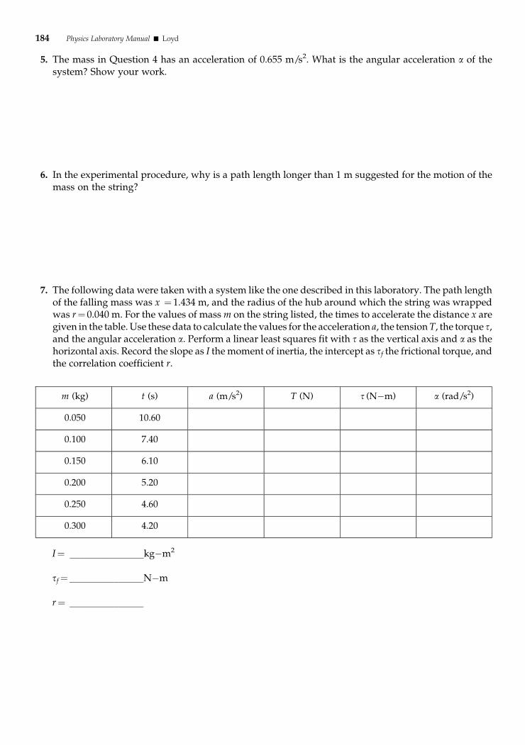
5. The mass in Question 4 has an acceleration of 0.655 m/s2. What is the angular acceleration a of thesystem? Show your work.
6. In the experimental procedure, why is a path length longer than 1 m suggested for the motion of themass on the string?
7. The following data were taken with a system like the one described in this laboratory. The path lengthof the falling mass was x ¼ 1.434 m, and the radius of the hub around which the string was wrappedwas r¼ 0.040 m. For the values of massm on the string listed, the times to accelerate the distance x aregiven in the table. Use these data to calculate the values for the acceleration a, the tensionT, the torque t,and the angular acceleration a. Perform a linear least squares fit with t as the vertical axis and a as thehorizontal axis. Record the slope as I the moment of inertia, the intercept as tf the frictional torque, andthe correlation coefficient r.
m (kg) t (s) a (m/s2) T (N) t (N�m) a (rad/s2)
0.050 10.60
0.100 7.40
0.150 6.10
0.200 5.20
0.250 4.60
0.300 4.20
I¼ _______________kg�m2
tf¼ _______________N�m
r¼ _______________
184 Physics Laboratory Manual n Loyd

Name . . . . . . . . . . . . . . . . . . . . . . . . . . . . . . . . . . . . . . . . . . . . . . . . . . . . . . . . . . . . . . . . . . . . . . . . . Section . . . . . . . . . . . . . . . . Date . . . . . . . . . . . . . . . .
Lab Partners . . . . . . . . . . . . . . . . . . . . . . . . . . . . . . . . . . . . . . . . . . . . . . . . . . . . . . . . . . . . . . . . . . . . . . . . . . . . . . . . . . . . . . . . . . . . . . . . . . . . . . . . . . . . . . . . . . . .
17 L A B O R A T O R Y 1 7 Moment of Inertia and Rotational Motion
L A B O R A T O R Y R E P O R T
COPYRIG
HTª
2008ThomsonBrooks/Cole
Data Table
M¼ kg R¼ m r¼ m x¼ m
m (kg) t1 (s) t2 (s) t3 (s) t4 (s)
Calculations Table
t (s) Std Err (s) a (m/s2) T (N) t (N�m) a (rad/s2)
I theo¼ kg�m2 I exp¼ kg�m2 tf¼ N�m r¼
185
S A M P L E C A L C U L A T I O N S1. Itheo¼½ MR2¼2. a¼ 2x/(t)2¼3. T¼m(g� a)¼
Q U E S T I O N S1. Calculate the percentage error of the experimental value Iexp compared to the theoretical value Itheo.
Comment on the accuracy of your experimental results based on this comparison.
2. For six data points, statistical theory states that there is a 0.1% probability (1 chance in 1000) ofobtaining a value of r ‡ 0.974 for uncorrelated data. What does your value of r imply about theagreement of your data with the theory?
3. Would there be any advantage to using a smaller mass m than was used in the laboratory? Whatwould be the disadvantage of doing that?
186 Physics Laboratory Manual n Loyd

4. Would there be any advantage to using a larger massm than was used in the laboratory? What wouldbe the disadvantage of doing that?
5. What amount of mass placed on the string would produce a torque equal to the value of the frictionaltorque tf?
COPYRIG
HTª
2008ThomsonBrooks/Cole
Laboratory 17 n Moment of Inertia and Rotational Motion 187

This page intentionally left blank

Archimedes’ Principle
O B J E C T I V E So Apply Archimedes’ principle to measurements of specific gravity.
o Determine the specific gravity of several metal objects that are denser than water, a cork that isless dense than water, and a liquid (alcohol).
E Q U I P M E N T L I S T. Laboratory balance, calibrated masses, 1000 mL beaker, string, alcohol
. Metal cylinders, and cork or piece of wood (to serve as unknowns)
T H E O R YIf the mass of an object is distributed uniformly, its density ro is defined as the mass m of the objectdivided by its volume V. In equation form this is
ro ¼ m=V ðEq: 1Þ
The SI units for density are kg/m3. Other commonly used units for density are the cgs system units g/cm3.The specific gravity is defined as the ratio of the density of an object to the density of water rw. Theequation for the specific gravity is given by
Specific gravity ¼ SG ¼ ro=rw ðEq: 2Þ
Specific gravity is a dimensionless quantity because it is the ratio of two densities. The density of waterin the cgs system is 1.000 g/cm3, and densities in that system are numerically equal to the specific gravitySG. Water has a density of 1000 kg/m3, and densities in the SI system are equal to SG� 103.
Archimedes’ principle states that an object placed in a fluid experiences an upward buoyant forceequal to the weight of fluid displaced by the object. The principle applies to both liquids and gases.In this laboratory, we will examine the application of the principle to liquids. An object floats if itsdensity is less than the density of the liquid in which it is placed. It sinks in the liquid until it displacesa weight of liquid equal to its own weight. The object is in equilibrium because its weight acts down-ward and a buoyant force acts upward. An object with density greater than the liquid in which it isplaced will sink to the bottom of the liquid. It experiences an upward buoyant force equal to the weightof the displaced fluid, but that is less than the weight of the object, and it sinks.
Physics Laboratory Manual n Loyd L A B O R A T O R Y 18
COPYRIG
HTª
2008ThomsonBrooks/Cole
189
ª 2008 Thomson Brooks/Cole, a part of TheThomson Corporation.Thomson, the Star logo, and Brooks/Cole are trademarks used herein under license. ALL RIGHTSRESERVED.No part of this workcovered by the copyright hereonmay be reproduced or used in any form or by any meansçgraphic, electronic, ormechanical, including photocopying, recording, taping,web distribution, informationstorage and retrieval systems,or in any othermannerçwithout the written permission of the publisher.
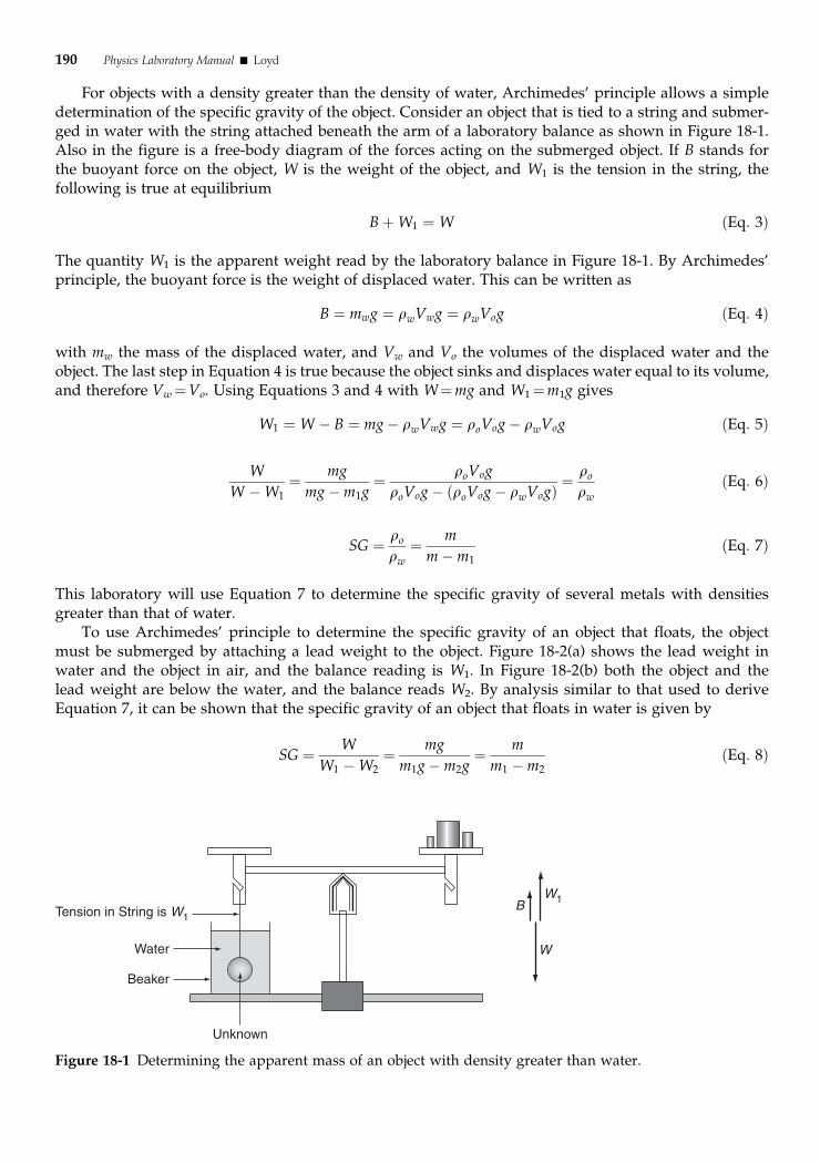
For objects with a density greater than the density of water, Archimedes’ principle allows a simpledetermination of the specific gravity of the object. Consider an object that is tied to a string and submer-ged in water with the string attached beneath the arm of a laboratory balance as shown in Figure 18-1.Also in the figure is a free-body diagram of the forces acting on the submerged object. If B stands forthe buoyant force on the object, W is the weight of the object, and W1 is the tension in the string, thefollowing is true at equilibrium
BþW1 ¼ W ðEq: 3Þ
The quantity W1 is the apparent weight read by the laboratory balance in Figure 18-1. By Archimedes’principle, the buoyant force is the weight of displaced water. This can be written as
B ¼ mwg ¼ rwVwg ¼ rwVog ðEq: 4Þ
with mw the mass of the displaced water, and Vw and Vo the volumes of the displaced water and theobject. The last step in Equation 4 is true because the object sinks and displaces water equal to its volume,and therefore Vw¼Vo. Using Equations 3 and 4 with W¼mg and W1¼m1g gives
W1 ¼ W � B ¼ mg� rwVwg ¼ roVog� rwVog ðEq: 5Þ
W
W �W1¼ mg
mg�m1g¼ roVog
roVog� ðroVog� rwVogÞ ¼rorw
ðEq: 6Þ
SG ¼ rorw
¼ m
m�m1ðEq: 7Þ
This laboratory will use Equation 7 to determine the specific gravity of several metals with densitiesgreater than that of water.
To use Archimedes’ principle to determine the specific gravity of an object that floats, the objectmust be submerged by attaching a lead weight to the object. Figure 18-2(a) shows the lead weight inwater and the object in air, and the balance reading is W1. In Figure 18-2(b) both the object and thelead weight are below the water, and the balance reads W2. By analysis similar to that used to deriveEquation 7, it can be shown that the specific gravity of an object that floats in water is given by
SG ¼ W
W1 �W2¼ mg
m1g�m2g¼ m
m1 �m2ðEq: 8Þ
Tension in String is W1
Water
Beaker
Unknown
BW1
W
Figure 18-1 Determining the apparent mass of an object with density greater than water.
190 Physics Laboratory Manual n Loyd

In Equation 8 m is the mass of the object, m1 is the apparent mass with the object in air and the leadweight submerged in water, and m2 is the apparent mass with the object and the lead weight bothsubmerged in water.
The specific gravity of a liquid can be determined by measuring the mass of some object m, theapparent mass of the object submerged in water mw, and the apparent mass of the object submerged inthe liquid mL. It is assumed that the object sinks in both liquids. By similar analysis as used to deriveEquation 7, it can be shown that the specific gravity of the liquid is given by
SGðliquidÞ ¼m�mL
m�mwðEq: 9Þ
E X P E R I M E N T A L P R O C E D U R EObject Density Greater than Water
1. Use the laboratory balance to determine the mass of each of the two unknown metal cylinders.Record these values as m in Data Table 1. The unknowns should have their metal type stamped onthem, or else ask your instructor for the metal type of the unknowns. Record the metal of theunknowns in Calculations Table 1.
2. Place a clamp on the laboratory table and screw a threaded rod in the clamp. Slide the rod into thehole designed for that purpose in the base of the laboratory balance. Adjust the height of the balanceabove the table to allow the 1000mL beaker to fit under the balance. Fill the beaker about three-fourthsfull of water.
3. Tie a piece of light string or thread around one of the unknowns and suspend it from one of the slotsin the left arm underneath the balance. Determine the apparent mass with the unknown suspendedcompletely below the surface of the water. Be sure that the unknown is not touching the side of thebeaker or is in any way supported by anything other than the string. Record the mass reading ofthe balance as m1 in Data Table 1.
4. Repeat Steps 1 through 3 for the second unknown.
5. From Appendix II obtain the known SG of the metal for each of the unknowns and record thosevalues in Data Table 1.
Object Density Less than Water
1. Using the laboratory balance, determine the mass of the cork and record it as m in Data Table 2.
2. Determine the apparent mass with the cork suspended in air and a lead weight tied below submergedin water as shown in Figure 18-2(a). Record that value as m1 in Data Table 2.
COPYRIG
HTª
2008ThomsonBrooks/Cole
W1
W W
W2
Bs
Ws
W
BW2
W1
Ws
Ws Ws
W
Bs
0
(a) (b)
Figure 18-2 Forces acting on an object held submerged by a lead weight.
Laboratory 18 n Archimedes’ Principle 191
3. Determine the apparent mass with both the cork and the lead weight submerged in water as shownin Figure 18-2(b). Record that value as m2 in Data Table 2.
Liquid Unknown
1. Use one of the unknown metal cylinders from the original procedure. Its mass m and its apparentmass in water have already been determined. Record those values in Data Table 3.
2. Use a very clean beaker and fill it about three-fourths full of alcohol. Determine the apparent mass ofthe metal cylinder in alcohol. Record it as mL in Data Table 3. Return the alcohol to its containerwhen you have finished with it. Be very careful not to have any spark or flame near the alcohol.
3. Repeat Steps 1 and 2 for the other unknown metal.
4. From Appendix II determine the known value of the specific gravity of alcohol and record it in DataTable 3.
C A L C U L A T I O N SDensity Greater than Water
1. Use Equation 7 to calculate the SG for each of the unknowns. Record the experimental values of thespecific gravity in Calculations Table 1.
2. Calculate the percentage error in your value of the SG for each of the unknowns compared to theknown values. Record them in Calculations Table 1.
Density Less than Water
1. Use Equation 8 to calculate the specific gravity SG for the cork and record it in Calculations Table 2.
Liquid Unknown
1. Use Equation 9 to determine the specific gravity of the alcohol for the two trials with the differentmetals. Record those values in Calculations Table 3.
2. Calculate the percentage error in each of the two measurements of the specific gravity of alcohol.Record the results in Calculations Table 3.
192 Physics Laboratory Manual n Loyd

Name . . . . . . . . . . . . . . . . . . . . . . . . . . . . . . . . . . . . . . . . . . . . . . . . . . . . . . . . . . . . . . . . . . . . . . . . . Section . . . . . . . . . . . . . . . . Date . . . . . . . . . . . . . . . .
18 L A B O R A T O R Y 1 8 Archimedes’ Principle
P R E - L A B O R A T O R Y A S S I G N M E N T1. What is the definition of density? What are its units?
2. What is specific gravity? What are its units?
3. State Archimedes’ principle.
4. The buoyant force on an object placed in a liquid is (a) always equal to the volume of the liquiddisplaced (b) always equal to the weight of the object (c) always equal to the weight of the liquiddisplaced (d) always less than the volume of the liquid displaced.
5. An object that sinks in water displaces a volume of water (a) equal to the object’s weight (b) equal tothe object’s volume (c) less than the object’s volume (d) greater than the object’s weight.
COPYRIG
HTª
2008ThomsonBrooks/Cole
193
6. An object that sinks in water has a mass in air of 0.0675 kg. Its apparent mass when submerged inwater, as in Figure 18-1, is 0.0424 kg. What is the specific gravity SG of the object? Consideringthe densities given in Appendix II, of what material is the object probably made? Show your work.
7. A piece of wood that floats on water has a mass of 0.0175 kg. A lead weight is tied to the wood, andthe apparent mass with the wood in air and the lead weight submerged in water is 0.0765 kg.The apparent mass with both the wood and the lead weight both submerged in water is 0.0452 kg.What is the specific gravity of the wood? Show your work.
8. An object has a mass in air of 0.0832 kg, apparent mass in water of 0.0673 kg, and apparent massin another liquid of 0.0718 kg. What is the specific gravity of the other liquid? Show your work.
194 Physics Laboratory Manual n Loyd

Name . . . . . . . . . . . . . . . . . . . . . . . . . . . . . . . . . . . . . . . . . . . . . . . . . . . . . . . . . . . . . . . . . . . . . . . . . Section . . . . . . . . . . . . . . . . Date . . . . . . . . . . . . . . . .
Lab Partners . . . . . . . . . . . . . . . . . . . . . . . . . . . . . . . . . . . . . . . . . . . . . . . . . . . . . . . . . . . . . . . . . . . . . . . . . . . . . . . . . . . . . . . . . . . . . . . . . . . . . . . . . . . . . . . . . . . .
18 L A B O R A T O R Y 1 8 Archimedes’ Principle
L A B O R A T O R Y R E P O R T
COPYRIG
HTª
2008ThomsonBrooks/Cole
Calculations Table 1
SG ¼ m
m�m1% Error
Data Table 1
Metal Known SG m (kg) m1 (kg)
Calculations Table 2
SG ¼ m
m1�m2
Data Table 2
m (kg) m1 (kg) m2 (kg)
Calculations Table 3
SG ¼ m�mL
m�mw% Error
Data Table 3
Metal m (kg) mw (kg) mL (kg)
Known SG of Alcohol¼
195
S A M P L E C A L C U L A T I O N S1. SG¼m/(m�m1)¼2. SG¼m/(m1�m2)¼3. SG¼ (m�mL)/(m�mw)
4. % Error¼ jE�Kj/K� (100%)¼
Q U E S T I O N S1. Do your data indicate that Archimedes’ principle is valid? State clearly the evidence for your answer.
2. An object with a specific gravity of 0.900 is placed in a liquid with a specific gravity of 0.900. Describeif the object will sink, float, or behave in some other way.
3. An object with a specific gravity of 0.850 is placed in water. What fraction of the object is below thesurface of the water?
4. Consider a swimmerwho swims first in a freshwater lake, and then swims in the ocean. Is the buoyantforce on her the same in both cases? If the buoyant force is different for the two cases, state which oneis greater and why.
196 Physics Laboratory Manual n Loyd

The Pendulum—Approximate SimpleHarmonic Motion
O B J E C T I V E So Investigate the dependence of the period T of a pendulum on the length L and the mass M of
the bob.
o Demonstrate that the period T of a pendulum depends slightly on the angular amplitude of theoscillation for large angles, but that the dependence is negligible for small angular amplitude ofoscillation.
o Determine an experimental value of the acceleration due to gravity g by comparing themeasuredperiod of a pendulum with the theoretical prediction.
E Q U I P M E N T L I S T. Pendulum clamp, string, and calibrated hooked masses, laboratory timer
. Protractor and meter stick
T H E O R YA mass M moving in one dimension is said to exhibit simple harmonic motion if its displacement xfrom some equilibrium position is described by a single sine or cosine function. This happens when theparticle is subjected to a force F directly proportional to the magnitude of the displacement and directedtoward the equilibrium position. In equation form this is
F ¼ �kx ðEq: 1Þ
The period T of the motion is the time for one complete oscillation, and it is determined by the mass Mand the constant k. The equation that describes the dependence of T on M and k is
T ¼ 2p
ffiffiffiffiffiM
k
rðEq: 2Þ
Physics Laboratory Manual n Loyd L A B O R A T O R Y 19
COPYRIG
HTª
2008ThomsonBrooks/Cole
197
ª 2008 Thomson Brooks/Cole, a part of TheThomson Corporation.Thomson, the Star logo, and Brooks/Cole are trademarks used herein under license. ALL RIGHTSRESERVED.No part of this workcovered by the copyright hereonmay be reproduced or used in any form or by any meansçgraphic, electronic, ormechanical, including photocopying, recording, taping,web distribution, informationstorage and retrieval systems,or in any othermannerçwithout the written permission of the publisher.
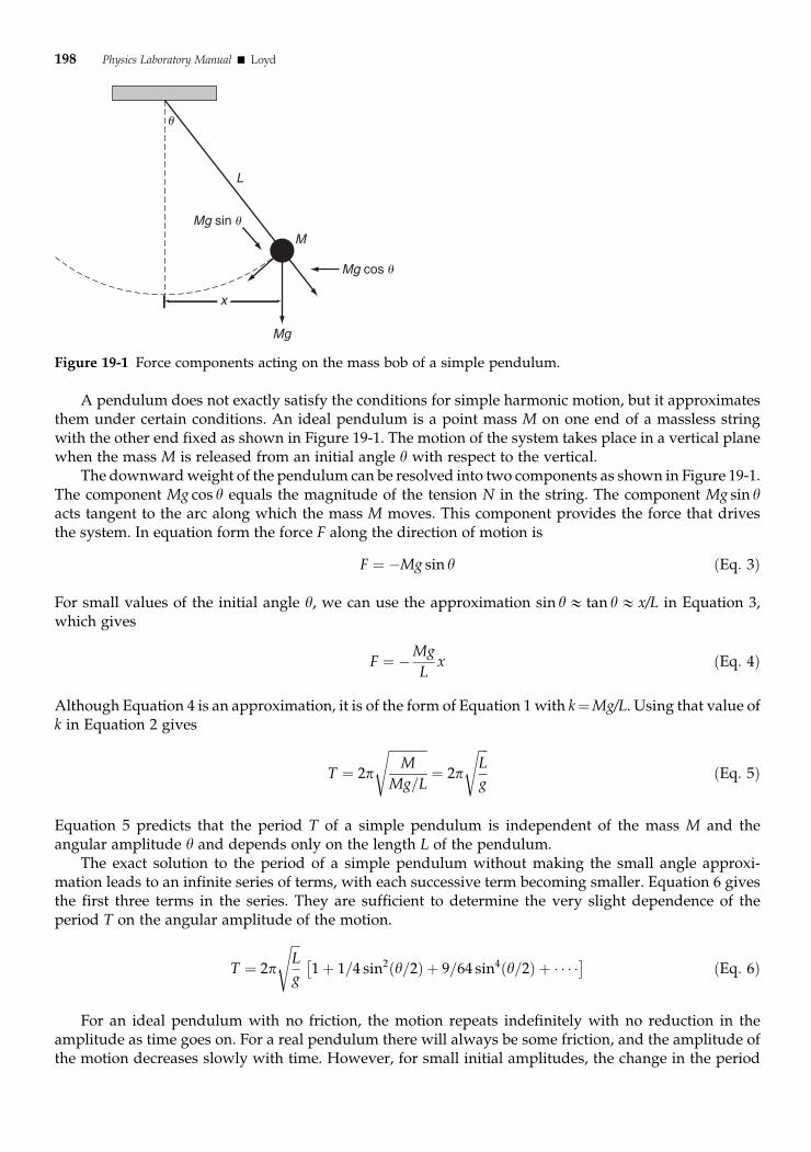
A pendulum does not exactly satisfy the conditions for simple harmonic motion, but it approximatesthem under certain conditions. An ideal pendulum is a point mass M on one end of a massless stringwith the other end fixed as shown in Figure 19-1. The motion of the system takes place in a vertical planewhen the mass M is released from an initial angle y with respect to the vertical.
The downwardweight of the pendulum can be resolved into two components as shown in Figure 19-1.The component Mg cos y equals the magnitude of the tension N in the string. The component Mg sin yacts tangent to the arc along which the mass M moves. This component provides the force that drivesthe system. In equation form the force F along the direction of motion is
F ¼ �Mg sin y ðEq: 3Þ
For small values of the initial angle y, we can use the approximation sin y& tan y& x/L in Equation 3,which gives
F ¼ �Mg
Lx ðEq: 4Þ
Although Equation 4 is an approximation, it is of the form of Equation 1 with k¼Mg/L. Using that value ofk in Equation 2 gives
T ¼ 2p
ffiffiffiffiffiffiffiffiffiffiffiffiM
Mg=L
s¼ 2p
ffiffiffiL
g
sðEq: 5Þ
Equation 5 predicts that the period T of a simple pendulum is independent of the mass M and theangular amplitude y and depends only on the length L of the pendulum.
The exact solution to the period of a simple pendulum without making the small angle approxi-mation leads to an infinite series of terms, with each successive term becoming smaller. Equation 6 givesthe first three terms in the series. They are sufficient to determine the very slight dependence of theperiod T on the angular amplitude of the motion.
T ¼ 2p
ffiffiffiL
g
s1þ 1=4 sin2ðy=2Þ þ 9=64 sin4ðy=2Þ þ � � � � � ðEq: 6Þ
For an ideal pendulum with no friction, the motion repeats indefinitely with no reduction in theamplitude as time goes on. For a real pendulum there will always be some friction, and the amplitude ofthe motion decreases slowly with time. However, for small initial amplitudes, the change in the period
L
MMg sin �
�
Mg
x
Mg cos �
Figure 19-1 Force components acting on the mass bob of a simple pendulum.
198 Physics Laboratory Manual n Loyd
COPYRIG
HTª
2008ThomsonBrooks/Cole
as the amplitude decreases is negligible. This fact is the basis for the pendulum clock. Pendulum clocks, inone form or another, have been used for more than 300 years. For more than 100 years, clockmakers havebuilt extremely accurate clocks by successfully employing devices to compensate for small changes in thelength of the pendulum caused by temperature variations.
E X P E R I M E N T A L P R O C E D U R ELength
1. The dependence of T on the length of the pendulum will be determined with a fixed mass and fixedangular amplitude. Place a 0.2000 kg hooked calibratedmass on a string with a loop in one end. Adjustthe position at which the other end of the string is clamped in the pendulum clamp until the distancefrom the point of support to the center of mass of the hooked mass is 1.0000 m. The length L of eachpendulum is from the point of support to the center of mass of the bob. The center of mass of thehookedmasses will usually not be in the center because the hookedmasses are not solid at the bottom.Estimate howmuch this tends to raise the position of the center of mass andmark the estimated centerof mass on each hooked mass.
2. Displace the pendulum 5.08 from the vertical and release it.Measure the timeDt for 10 complete periodsof motion and record that value in Data Table 1. It is best to set the pendulum inmotion, and then beginthe timer as it reaches themaximumdisplacement, counting 10 round trips back to that position. Repeatthis process twomore times for a total of three trials with this same length. The pendulum shouldmovein a plane as it swings. If the mass moves in an elliptical path, it will lead to error.
3. Repeat the procedure of Step 2, using the same mass and an angle of 5.08 for pendulum lengths of0.8000, 0.6000, 0.5000, 0.3000, 0.2000, and 0.1000meters. Do three trials at each length. The length of thependulum is from the point of support to the center of mass of the hooked mass.
Mass
1. The dependence of T on M will be determined with the length L and amplitude y held constant.Place a 0.0500 kg mass on the end of the string and adjust the point of support of the string untilthe pendulum length is 1.0000 m. Displace the mass 5.08 and release it. Measure the time Dt for10 complete periods of the motion and record it in Data Table 2. Repeat the procedure two moretimes for a total of three trials.
2. Keep the length constant at L¼ 1.0000 m and repeat the procedure above for M of 0.1000, 0.2000,and 0.5000 kg. Because L is from the point of support to the center of mass, you will need to makeslight adjustments in the string length to keep L constant for the different masses.
Amplitude
1. The dependence of T on amplitude of the motion will be determined with L and M constant.Construct a pendulum with L¼ 1.000 m and M¼ 0.200 kg. Measure the time Dt for 10 completeperiods with amplitude 5.08. Repeat two more times for a total of three trials at this amplitude. Recordall results in Data Table 3.
2. Repeat the procedure above for amplitudes of 10.08, 20.08, 30.08, and 45.08. Do three trials for eachamplitude and record the results in Data Table 3.
C A L C U L A T I O N SLength
1. Calculate the mean Dt and standard error at of the three trials for each of the lengths. Record thoseresults in Calculations Table 1.
Laboratory 19 n The Pendulum—Approximate Simple Harmonic Motion 199
2. Calculate the period T from T ¼ Dt=10 and record it in Calculations Table 1.
3. According to Equation 5 the period T should be proportional toffiffiffiL
p. For each of the values of L
calculateffiffiffiL
pand record the results in Calculations Table 1. Perform a linear least squares fit with T
as the vertical axis andffiffiffiL
pas the horizontal axis. By Equation 5 the slope of this fit should equal 2p=
ffiffiffig
p.
Equate the slope determined from the fit to 2p=ffiffiffig
p, treating g as unknown. Solve this equation for g and
record that value as gexp in Calculations Table 1. Also record the value of the correlation coefficient rfor the fit.
Mass
1. Calculate the mean Dt and standard error at of the three trials for each of the masses. Record thoseresults in Calculations Table 2.
2. Calculate the period T from T ¼ Dt=10 and record in Calculations Table 2.
Amplitude
1. Calculate the mean Dt and standard error at for the three trials at each amplitude. Record the results inCalculations Table 3.
2. Calculate T ¼ Dt=10 and record the results in Calculations Table 3 as Texp.
3. Equation 6 is the theoretical prediction for how the period T should depend on the amplitude.Use L¼ 1.000 m and M¼ 0.200 kg in Equation 6 to calculate the T predicted for the values of y.Record them in Calculations Table 3 as Ttheo.
4. For the experimental values of the period Texp calculate the ratio of the period at the other angles tothe period at y¼ 5.08. Call this ratio
�TexpðyÞ=Texpð5:0�Þ
�. Record these values in Calculations Table 3.
5. For the theoretical values of the period Ttheo calculate the ratio of the period at the other angles to theperiod at y¼ 5.08. Call this ratio
�TtheoðyÞ=Ttheoð5:0�Þ
�. Record these values in Calculations Table 3.
G R A P H S1. Consider the data for the dependence of the period T on the length L. Graph the period T as the
vertical axis andffiffiffiL
pas the horizontal axis. Also show on the graph the straight line obtained by
the linear fit to the data.
2. Consider the data for the dependence of the period T on the mass M. Graph the period T as thevertical axis and the mass M as the horizontal axis.
200 Physics Laboratory Manual n Loyd
Name . . . . . . . . . . . . . . . . . . . . . . . . . . . . . . . . . . . . . . . . . . . . . . . . . . . . . . . . . . . . . . . . . . . . . . . . . Section . . . . . . . . . . . . . . . . Date . . . . . . . . . . . . . . . .
19 L A B O R A T O R Y 1 9 The Pendulum—Approximate SimpleHarmonic Motion
P R E - L A B O R A T O R Y A S S I G N M E N T1. What is the requirement for a force to produce simple harmonic motion?
2. A particle of mass M¼ 1.35 kg is subject to a force F¼�0.850 x, where x is the displacement ofthe particle from equilibrium. The units of force F are Newtons, and the units of x are meters. Whatis the period T of its motion? Show your work.
3. A simple pendulum of length L¼ 0.800 m has a mass M¼ 0.250 kg. What is the tension in the stringwhen it is at an angle y¼ 12.58? Show your work.
4. In Question 3, what is the component of the weight of M that is directed along the arc of the motionof M? Show your work.
COPYRIG
HTª
2008ThomsonBrooks/Cole
201

5. What is the period T of the motion of the pendulum in Question 3? Assume that the period isindependent of y. Show your work.
6. What would be the period T of the pendulum in Question 3 if L was unchanged but M¼ 0.500 kg?Assume that the period is independent of y. Show your work.
7. Determine the period T of the pendulum in Question 3 if everything else stays the same, but y¼ 45.08.Do not assume that the period is independent of y. Show your work.
202 Physics Laboratory Manual n Loyd

Name . . . . . . . . . . . . . . . . . . . . . . . . . . . . . . . . . . . . . . . . . . . . . . . . . . . . . . . . . . . . . . . . . . . . . . . . . Section . . . . . . . . . . . . . . . . Date . . . . . . . . . . . . . . . .
Lab Partners . . . . . . . . . . . . . . . . . . . . . . . . . . . . . . . . . . . . . . . . . . . . . . . . . . . . . . . . . . . . . . . . . . . . . . . . . . . . . . . . . . . . . . . . . . . . . . . . . . . . . . . . . . . . . . . . . . . .
19 L A B O R A T O R Y 1 9 The Pendulum—Approximate SimpleHarmonic Motion
L A B O R A T O R Y R E P O R T
Data and Calculations Table 1
L (m) Dt1 (s) Dt2 (s) Dt3 (s) Dt (s) at (s) T (s)ffiffiffiL
p(ffiffiffiffiffim
p)
1.0000
0.8000
0.6000
0.5000
0.3000
0.2000
0.1000
Slope¼ gexp¼ m/s2 r¼
Data and Calculations Table 2
M (kg) Dt1 (s) Dt2 (s) Dt3 (s) Dt (s) at (s) T (s)
0.0500
0.1000
0.2000
0.5000
COPYRIG
HTª
2008ThomsonBrooks/Cole
203
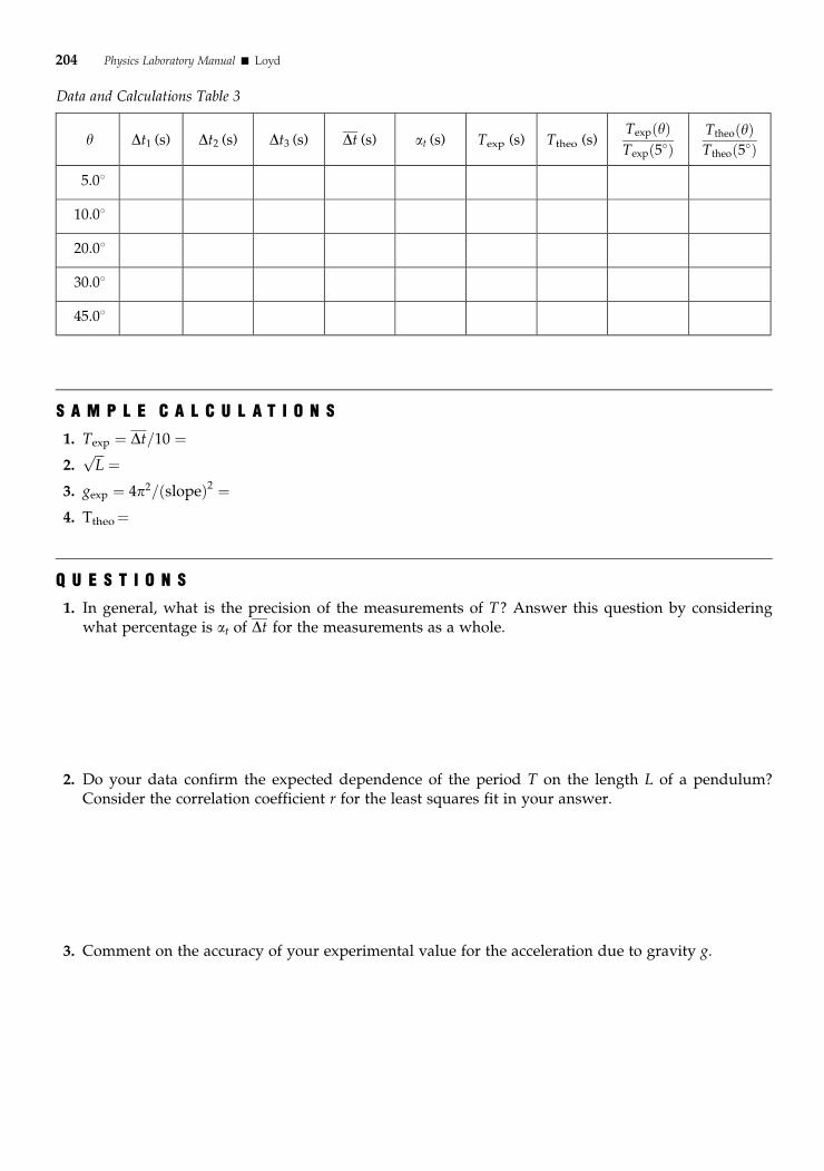
Data and Calculations Table 3
y Dt1 (s) Dt2 (s) Dt3 (s) Dt (s) at (s) Texp (s) Ttheo (s)TexpðyÞTexpð5�Þ
TtheoðyÞTtheoð5�Þ
5.08
10.08
20.08
30.08
45.08
S A M P L E C A L C U L A T I O N S1. Texp ¼ Dt=10 ¼2.
ffiffiffiL
p ¼3. gexp ¼ 4p2=ðslopeÞ2 ¼4. Ttheo¼
Q U E S T I O N S1. In general, what is the precision of the measurements of T? Answer this question by considering
what percentage is at of Dt for the measurements as a whole.
2. Do your data confirm the expected dependence of the period T on the length L of a pendulum?Consider the correlation coefficient r for the least squares fit in your answer.
3. Comment on the accuracy of your experimental value for the acceleration due to gravity g.
204 Physics Laboratory Manual n Loyd

4. What does the theory predict for the shape of the graph of period T versus M? Do your data confirmthis expectation? Calculate the mean and standard error of the periods for the four masses andcomment on how this relates to mass independence of T.
5. Do your measured values for the period T as a function of the amplitude y confirm the theoreticalpredictions? State clearly what is expected and what your data show.
6. The values of T were determined by measuring the time for 10 periods. Why is the time for morethan one period measured? If there is an advantage to measuring for 10 periods, why not measure for1000 periods?
COPYRIG
HTª
2008ThomsonBrooks/Cole
Laboratory 19 n The Pendulum—Approximate Simple Harmonic Motion 205

This page intentionally left blank

Simple Harmonic Motion—Mass on a Spring
O B J E C T I V E So Directly determine the spring constant k of a spring by measuring the elongation versus applied
force.
o Determine the spring constant k from measurements of the period T of oscillation for differentvalues of mass.
o Investigate the dependence of the period T of oscillation of a mass on a spring on the value of themass and on the amplitude of the motion.
E Q U I P M E N T L I S T. Spring, masking tape, laboratory timer, meter stick, table clamps, and rods
. Right-angle clamps, laboratory balance, and calibrated hooked masses
T H E O R YAmass that experiences a restoring force proportional to its displacement from an equilibrium position issaid to obey Hooke’s law. In equation form this relationship can be expressed as
F ¼ �ky ðEq: 1Þ
where k is a constant with dimensions of N/m. The negative sign indicates that the force is in the oppositedirection of the displacement. If a spring exerts the force, the constant k is the spring constant.
A force described by Equation 1 will produce an oscillatory motion called simple harmonic motionbecause it can be described by a single sine or cosine function of time. A mass displaced from itsequilibrium position by some value A, and then released, will oscillate about the equilibrium position.Its displacement y from the equilibrium position will range between y¼A and y¼�A with A called theamplitude of the motion. For the initial conditions described above, the displacement y as a function oftime t is given by
y ¼ A cosðotþ fÞ ðEq: 2Þ
Physics Laboratory Manual n Loyd L A B O R A T O R Y 20
COPYRIG
HTª
2008ThomsonBrooks/Cole
207
ª 2008 Thomson Brooks/Cole, a part of TheThomson Corporation.Thomson, the Star logo, and Brooks/Cole are trademarks used herein under license. ALL RIGHTSRESERVED.No part of this workcovered by the copyright hereonmay be reproduced or used in any form or by any meansçgraphic, electronic, ormechanical, including photocopying, recording, taping,web distribution, informationstorage and retrieval systems,or in any othermannerçwithout the written permission of the publisher.
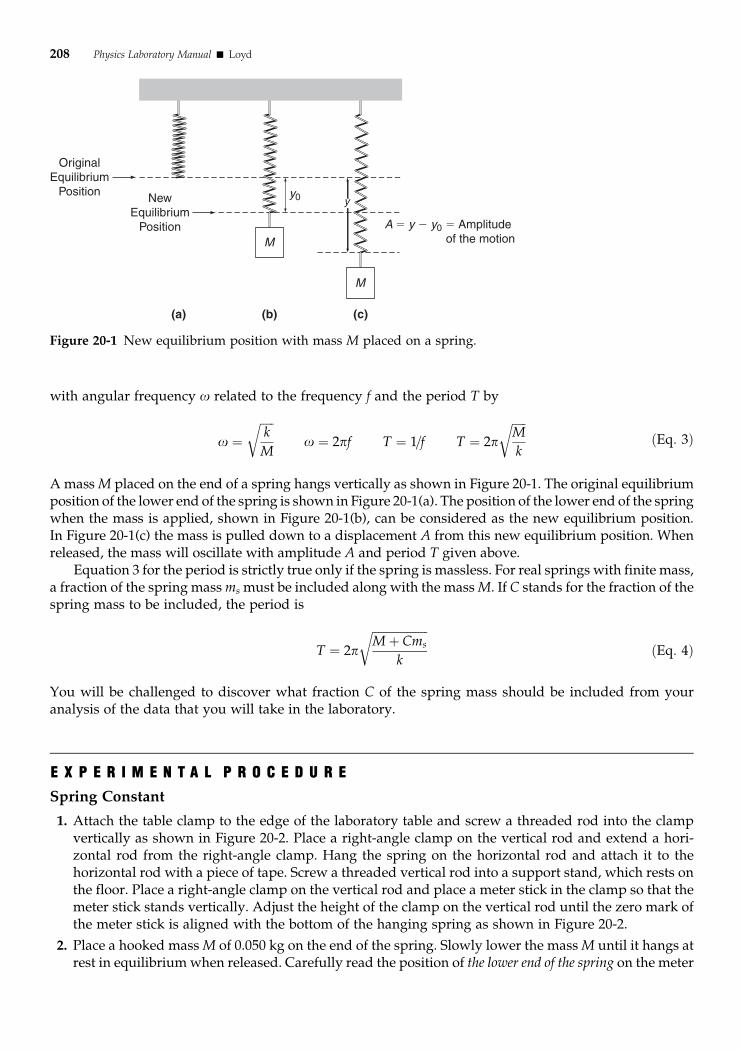
with angular frequency o related to the frequency f and the period T by
o ¼ffiffiffiffiffik
M
ro ¼ 2pf T ¼ 1=f T ¼ 2p
ffiffiffiffiffiM
k
rðEq: 3Þ
AmassM placed on the end of a spring hangs vertically as shown in Figure 20-1. The original equilibriumposition of the lower end of the spring is shown in Figure 20-1(a). The position of the lower end of the springwhen the mass is applied, shown in Figure 20-1(b), can be considered as the new equilibrium position.In Figure 20-1(c) the mass is pulled down to a displacement A from this new equilibrium position. Whenreleased, the mass will oscillate with amplitude A and period T given above.
Equation 3 for the period is strictly true only if the spring is massless. For real springs with finite mass,a fraction of the spring massms must be included along with the massM. If C stands for the fraction of thespring mass to be included, the period is
T ¼ 2p
ffiffiffiffiffiffiffiffiffiffiffiffiffiffiffiffiffiffiffiMþ Cms
k
rðEq: 4Þ
You will be challenged to discover what fraction C of the spring mass should be included from youranalysis of the data that you will take in the laboratory.
E X P E R I M E N T A L P R O C E D U R ESpring Constant
1. Attach the table clamp to the edge of the laboratory table and screw a threaded rod into the clampvertically as shown in Figure 20-2. Place a right-angle clamp on the vertical rod and extend a hori-zontal rod from the right-angle clamp. Hang the spring on the horizontal rod and attach it to thehorizontal rod with a piece of tape. Screw a threaded vertical rod into a support stand, which rests onthe floor. Place a right-angle clamp on the vertical rod and place a meter stick in the clamp so that themeter stick stands vertically. Adjust the height of the clamp on the vertical rod until the zero mark ofthe meter stick is aligned with the bottom of the hanging spring as shown in Figure 20-2.
2. Place a hooked massM of 0.050 kg on the end of the spring. Slowly lower the massM until it hangs atrest in equilibriumwhen released. Carefully read the position of the lower end of the spring on the meter
M
A � y � y0 � Amplitude of the motion
y0 y
OriginalEquilibrium
Position
(c)(b)(a)
NewEquilibrium
Position
M
Figure 20-1 New equilibrium position with mass M placed on a spring.
208 Physics Laboratory Manual n Loyd
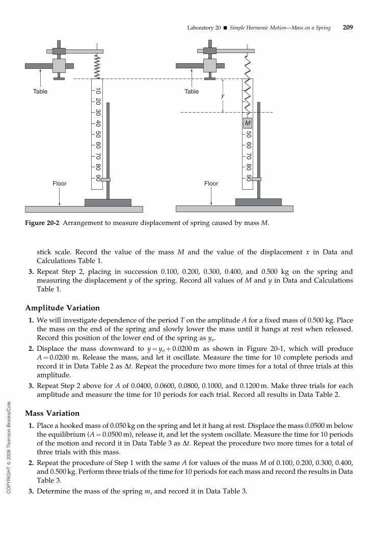
stick scale. Record the value of the mass M and the value of the displacement x in Data andCalculations Table 1.
3. Repeat Step 2, placing in succession 0.100, 0.200, 0.300, 0.400, and 0.500 kg on the spring andmeasuring the displacement y of the spring. Record all values of M and y in Data and CalculationsTable 1.
Amplitude Variation
1. We will investigate dependence of the period T on the amplitude A for a fixed mass of 0.500 kg. Placethe mass on the end of the spring and slowly lower the mass until it hangs at rest when released.Record this position of the lower end of the spring as yo.
2. Displace the mass downward to y¼ yoþ 0.0200m as shown in Figure 20-1, which will produceA¼ 0.0200 m. Release the mass, and let it oscillate. Measure the time for 10 complete periods andrecord it in Data Table 2 as Dt. Repeat the procedure two more times for a total of three trials at thisamplitude.
3. Repeat Step 2 above for A of 0.0400, 0.0600, 0.0800, 0.1000, and 0.1200m. Make three trials for eachamplitude and measure the time for 10 periods for each trial. Record all results in Data Table 2.
Mass Variation
1. Place a hooked mass of 0.050 kg on the spring and let it hang at rest. Displace the mass 0.0500 m belowthe equilibrium (A¼ 0.0500m), release it, and let the system oscillate. Measure the time for 10 periodsof the motion and record it in Data Table 3 as Dt. Repeat the procedure two more times for a total ofthree trials with this mass.
2. Repeat the procedure of Step 1 with the same A for values of the mass M of 0.100, 0.200, 0.300, 0.400,and 0.500 kg. Perform three trials of the time for 10 periods for eachmass and record the results in DataTable 3.
3. Determine the mass of the spring ms and record it in Data Table 3.COPYRIG
HTª
2008ThomsonBrooks/Cole
9080
7060
50
9080
7060
5040
3020
10
Floor Floor
Tabley
M
Table
Figure 20-2 Arrangement to measure displacement of spring caused by mass M.
Laboratory 20 n Simple Harmonic Motion—Mass on a Spring 209
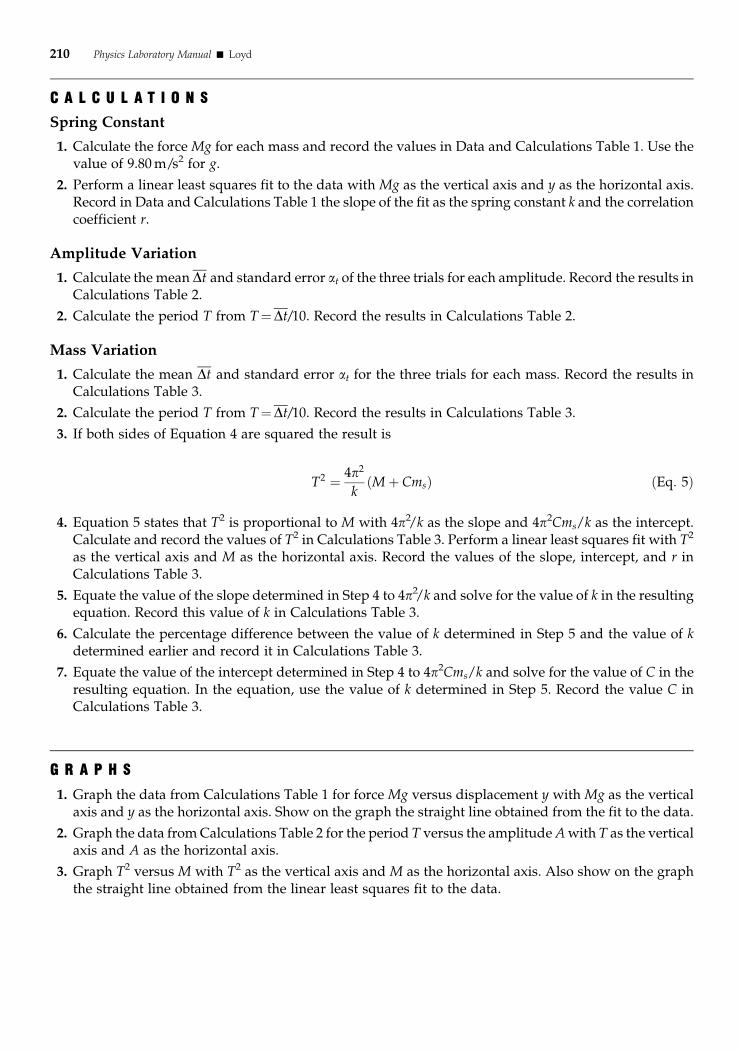
C A L C U L A T I O N SSpring Constant
1. Calculate the force Mg for each mass and record the values in Data and Calculations Table 1. Use thevalue of 9.80m/s2 for g.
2. Perform a linear least squares fit to the data with Mg as the vertical axis and y as the horizontal axis.Record in Data and Calculations Table 1 the slope of the fit as the spring constant k and the correlationcoefficient r.
Amplitude Variation
1. Calculate the mean Dt and standard error at of the three trials for each amplitude. Record the results inCalculations Table 2.
2. Calculate the period T from T¼Dt/10. Record the results in Calculations Table 2.
Mass Variation
1. Calculate the mean Dt and standard error at for the three trials for each mass. Record the results inCalculations Table 3.
2. Calculate the period T from T¼Dt/10. Record the results in Calculations Table 3.
3. If both sides of Equation 4 are squared the result is
T2 ¼ 4p2
kðMþ CmsÞ ðEq: 5Þ
4. Equation 5 states that T2 is proportional to M with 4p2/k as the slope and 4p2Cms/k as the intercept.Calculate and record the values of T2 in Calculations Table 3. Perform a linear least squares fit with T2
as the vertical axis and M as the horizontal axis. Record the values of the slope, intercept, and r inCalculations Table 3.
5. Equate the value of the slope determined in Step 4 to 4p2/k and solve for the value of k in the resultingequation. Record this value of k in Calculations Table 3.
6. Calculate the percentage difference between the value of k determined in Step 5 and the value of kdetermined earlier and record it in Calculations Table 3.
7. Equate the value of the intercept determined in Step 4 to 4p2Cms/k and solve for the value of C in theresulting equation. In the equation, use the value of k determined in Step 5. Record the value C inCalculations Table 3.
G R A P H S1. Graph the data from Calculations Table 1 for force Mg versus displacement y with Mg as the vertical
axis and y as the horizontal axis. Show on the graph the straight line obtained from the fit to the data.
2. Graph the data fromCalculations Table 2 for the period T versus the amplitudeAwith T as the verticalaxis and A as the horizontal axis.
3. Graph T2 versus M with T2 as the vertical axis and M as the horizontal axis. Also show on the graphthe straight line obtained from the linear least squares fit to the data.
210 Physics Laboratory Manual n Loyd
Name . . . . . . . . . . . . . . . . . . . . . . . . . . . . . . . . . . . . . . . . . . . . . . . . . . . . . . . . . . . . . . . . . . . . . . . . . Section . . . . . . . . . . . . . . . . Date . . . . . . . . . . . . . . . .
20 L A B O R A T O R Y 2 0 Simple Harmonic Motion—Mass on a Spring
P R E - L A B O R A T O R Y A S S I G N M E N T1. Describe in words and give an equation for the kind of force that produces simple harmonic motion.
2. Other than the type of force that produces it, what characterizes simple harmonic motion?
3. A spring has a spring constant k¼ 8.75 N/m. If the spring is displaced 0.150 m from its equilibriumposition, what is the force that the spring exerts? Show your work.
4. A spring of constant k¼ 11.75 N/m is hung vertically. A 0.500 kg mass is suspended from the spring.What is the displacement of the end of the spring due to the weight of the 0.500 kg mass? Show yourwork.
COPYRIG
HTª
2008ThomsonBrooks/Cole
211

5. A spring with a mass on the end of it hangs in equilibrium a distance of 0.4200 m above the floor. Themass is pulled down a distance 0.0600m below the original position, released, and allowed tooscillate. How high above the floor is the mass at the highest point in its oscillation? Show your work.
6. Amassless spring has a spring constant of k¼ 7.85 N/m. A massM¼ 0.425 kg is placed on the spring,and it is allowed to oscillate. What is the period T of oscillation? Show your work.
7. Amassless spring of k¼ 6.45N/m has a massM¼ 0.300 kg on the end of the spring. The mass is pulleddown 0.0500m and released. What is the period T of the oscillation?What is the period T if the mass ispulled down 0.1000m and released? State clearly the reasoning for your answer.
212 Physics Laboratory Manual n Loyd

Name . . . . . . . . . . . . . . . . . . . . . . . . . . . . . . . . . . . . . . . . . . . . . . . . . . . . . . . . . . . . . . . . . . . . . . . . . Section . . . . . . . . . . . . . . . . Date . . . . . . . . . . . . . . . .
Lab Partners . . . . . . . . . . . . . . . . . . . . . . . . . . . . . . . . . . . . . . . . . . . . . . . . . . . . . . . . . . . . . . . . . . . . . . . . . . . . . . . . . . . . . . . . . . . . . . . . . . . . . . . . . . . . . . . . . . . .
20 L A B O R A T O R Y 2 0 Simple Harmonic Motion—Mass on a Spring
L A B O R A T O R Y R E P O R T
COPYRIG
HTª
2008ThomsonBrooks/Cole
Data and Calculations Table 1
M (kg) Mg (N) y (m) k (N/m) r
0.050
0.100
0.200
0.300
0.400
0.500
Data and Calculations Table 2 yo¼ _______________ m
A (m) Dt1 (s) Dt2 (s) Dt3 (s) Dt (s) at (s) T (s)
0.0200
0.0400
0.0600
0.0800
0.1000
0.1200
213
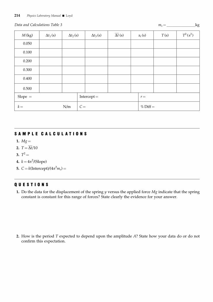
S A M P L E C A L C U L A T I O N S1. Mg¼2. T¼Dt/10
3. T2¼4. k¼ 4p2/(Slope)
5. C¼ k(Intercept)/(4p2ms)¼
Q U E S T I O N S1. Do the data for the displacement of the spring y versus the applied force Mg indicate that the spring
constant is constant for this range of forces? State clearly the evidence for your answer.
2. How is the period T expected to depend upon the amplitude A? State how your data do or do notconfirm this expectation.
Data and Calculations Table 3 ms¼ _______________kg
M (kg) Dt1 (s) Dt2 (s) Dt3 (s) Dt (s) at (s) T (s) T2 (s2)
0.050
0.100
0.200
0.300
0.400
0.500
Slope ¼ Intercept¼ r¼
k¼ N/m C¼ %Diff¼
214 Physics Laboratory Manual n Loyd

3. Consider the value you obtained for C. If you express that fraction as a whole number fraction, whichof the following would best fit your data? (½ �̂̄ ¼ �̂̇ )
4. Calculate T predicted by Equation 3 forM¼ 0.050 kg. Calculate T predicted by Equation 4with the sameM and your value of C. What is the percentage difference between these two values of T? Do thesame calculations for M¼ 0.500 kg. For which case are the percentage differences greater and whyare they greater?
5. The determination of T was done by measuring for 10 periods. Why was the time for more than oneperiod measured? If there is an advantage to measuring for 10 periods, why not measure for 1000periods?
COPYRIG
HTª
2008ThomsonBrooks/Cole
Laboratory 20 n Simple Harmonic Motion—Mass on a Spring 215

This page intentionally left blank

Standing Waves on a String
O B J E C T I V E So Demonstrate formation of standing waves on a string from the interference of traveling waves
traveling in opposite directions.
o Determine the tension T in the string required to produce standing waves.
o Investigate the relationship between tension T and the wavelength l of the wave.
o Determine an experimental value for the frequency f of the wave and compare it to the knownvalue of 120Hz.
E Q U I P M E N T L I S T. String vibrator (60Hz AC), string, clamps, pulley, support rods, meter stick
. Mass holder, slotted masses
. Laboratory balance capable of measuring to 0.00001 kg (one for class)
T H E O R YWaves are one means by which energy can be transported. Waves on a string are an example of transversewaves. These are waves in which individual particles of the medium (in this case the string) moveperpendicular or transverse to energy moving along the string. In Figure 21-1 a string tied to a vibrator atone end passes over a pulley, and the weight of masses on the other end provides tension T in the string.The vibrator moves up and down at a frequency f, which causes a wave of that same frequency topropagate down the string. The vibrator used in this laboratory is driven by an electromagnet at a fre-quency of 60Hz, but because the electromagnet attracts the steel blade twice in each cycle, the vibratorfrequency is 120Hz.
The point at which the string passes over the pulley is a fixed point, and the wave is reflected from thatpoint. Thus the string is a medium in which two waves of the same speed, frequency, and wavelengthtravel in the opposite direction. These two waves will interfere with each other to produce a standingwave when the proper relationship exists between the string length L and the wavelength l of the wave.When a standing wave is produced, its characteristic features are the existence of nodes and antinodesat points along the string. A node N is a point for which there is no displacement of the string from itsequilibrium position. An antinode A is a point on the string for which the amplitude of vibration is amaximum at all times. To form a standing wave a node must occur at each end of the string, and anantinode must occur between each node. The distance between nodes is l/2 or one-half of a wavelengthof the wave. In terms of the string length L, a standing wave is possible when
Physics Laboratory Manual n Loyd L A B O R A T O R Y 21
COPYRIG
HTª
2008ThomsonBrooks/Cole
217
ª 2008 Thomson Brooks/Cole, a part of TheThomson Corporation.Thomson, the Star logo, and Brooks/Cole are trademarks used herein under license. ALL RIGHTSRESERVED.No part of this workcovered by the copyright hereonmay be reproduced or used in any form or by any meansçgraphic, electronic, ormechanical, including photocopying, recording, taping,web distribution, informationstorage and retrieval systems,or in any othermannerçwithout the written permission of the publisher.
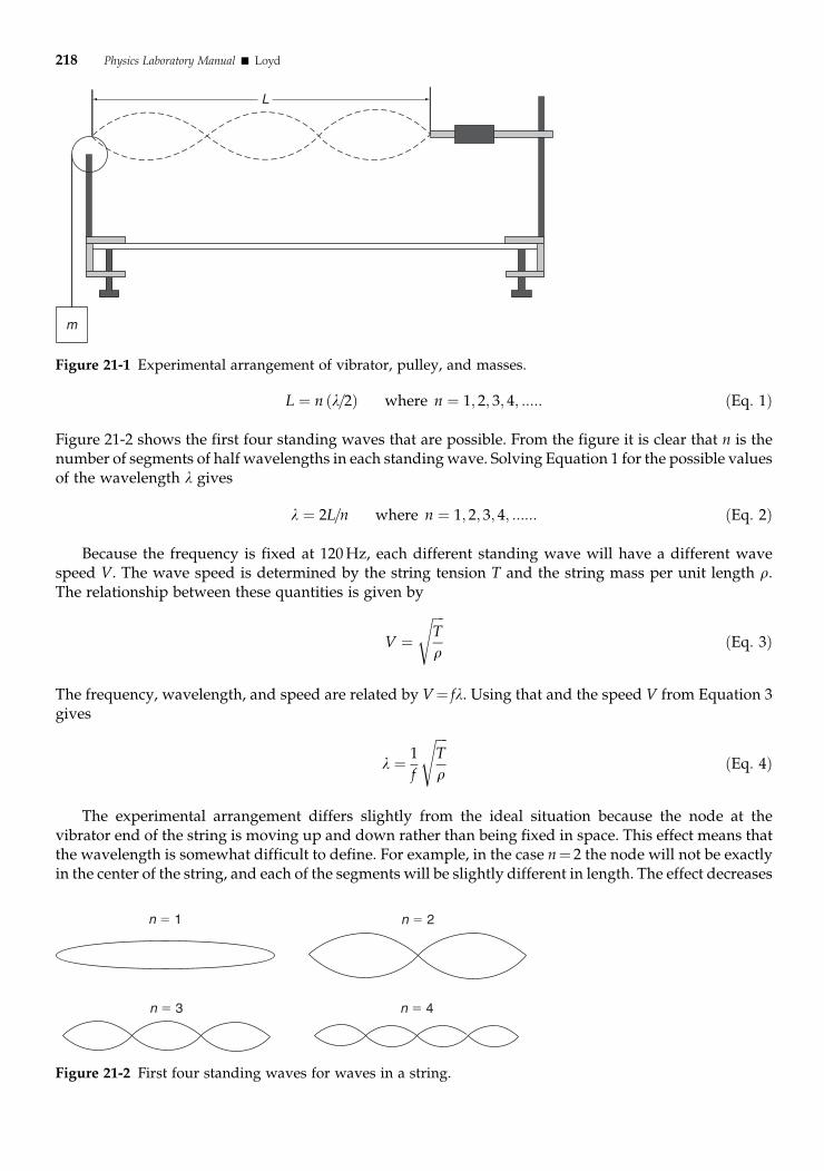
L ¼ n ðl=2Þ where n ¼ 1; 2; 3; 4; ::::: ðEq: 1Þ
Figure 21-2 shows the first four standing waves that are possible. From the figure it is clear that n is thenumber of segments of half wavelengths in each standingwave. Solving Equation 1 for the possible valuesof the wavelength l gives
l ¼ 2L=n where n ¼ 1; 2; 3; 4; :::::: ðEq: 2Þ
Because the frequency is fixed at 120Hz, each different standing wave will have a different wavespeed V. The wave speed is determined by the string tension T and the string mass per unit length r.The relationship between these quantities is given by
V ¼ffiffiffiffiT
r
sðEq: 3Þ
The frequency, wavelength, and speed are related by V¼ fl. Using that and the speed V from Equation 3gives
l ¼ 1
f
ffiffiffiffiT
r
sðEq: 4Þ
The experimental arrangement differs slightly from the ideal situation because the node at thevibrator end of the string is moving up and down rather than being fixed in space. This effect means thatthe wavelength is somewhat difficult to define. For example, in the case n¼ 2 the node will not be exactlyin the center of the string, and each of the segments will be slightly different in length. The effect decreases
L
m
Figure 21-1 Experimental arrangement of vibrator, pulley, and masses.
n � 1 n � 2
n � 3 n � 4
Figure 21-2 First four standing waves for waves in a string.
218 Physics Laboratory Manual n Loyd
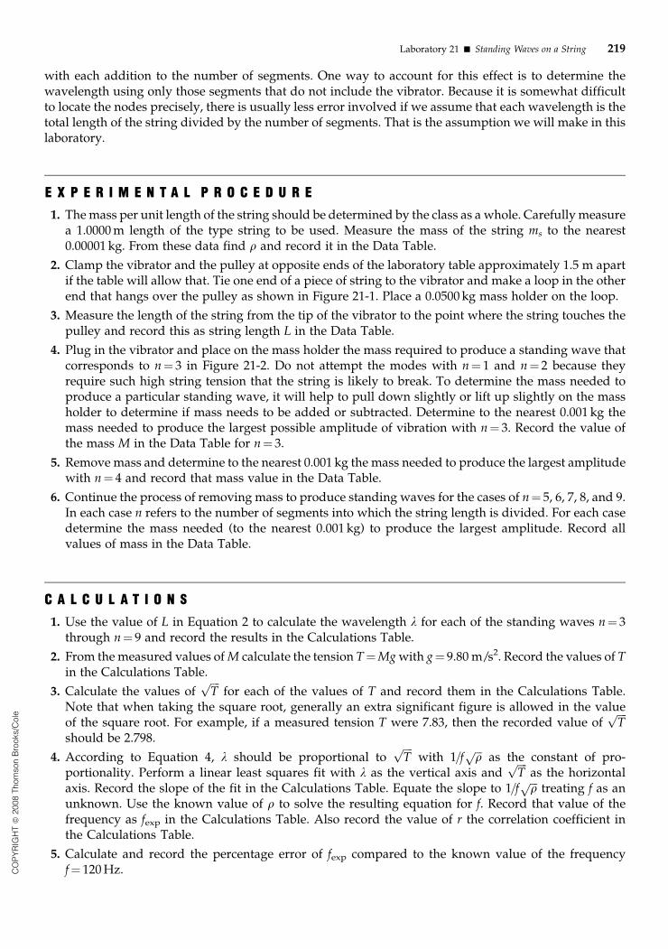
with each addition to the number of segments. One way to account for this effect is to determine thewavelength using only those segments that do not include the vibrator. Because it is somewhat difficultto locate the nodes precisely, there is usually less error involved if we assume that each wavelength is thetotal length of the string divided by the number of segments. That is the assumption we will make in thislaboratory.
E X P E R I M E N T A L P R O C E D U R E1. Themass per unit length of the string should be determined by the class as a whole. Carefullymeasure
a 1.0000m length of the type string to be used. Measure the mass of the string ms to the nearest0.00001 kg. From these data find r and record it in the Data Table.
2. Clamp the vibrator and the pulley at opposite ends of the laboratory table approximately 1.5 m apartif the table will allow that. Tie one end of a piece of string to the vibrator and make a loop in the otherend that hangs over the pulley as shown in Figure 21-1. Place a 0.0500 kg mass holder on the loop.
3. Measure the length of the string from the tip of the vibrator to the point where the string touches thepulley and record this as string length L in the Data Table.
4. Plug in the vibrator and place on the mass holder the mass required to produce a standing wave thatcorresponds to n¼ 3 in Figure 21-2. Do not attempt the modes with n¼ 1 and n¼ 2 because theyrequire such high string tension that the string is likely to break. To determine the mass needed toproduce a particular standing wave, it will help to pull down slightly or lift up slightly on the massholder to determine if mass needs to be added or subtracted. Determine to the nearest 0.001 kg themass needed to produce the largest possible amplitude of vibration with n¼ 3. Record the value ofthe mass M in the Data Table for n¼ 3.
5. Remove mass and determine to the nearest 0.001 kg the mass needed to produce the largest amplitudewith n¼ 4 and record that mass value in the Data Table.
6. Continue the process of removing mass to produce standing waves for the cases of n¼ 5, 6, 7, 8, and 9.In each case n refers to the number of segments into which the string length is divided. For each casedetermine the mass needed (to the nearest 0.001 kg) to produce the largest amplitude. Record allvalues of mass in the Data Table.
C A L C U L A T I O N S1. Use the value of L in Equation 2 to calculate the wavelength l for each of the standing waves n¼ 3
through n¼ 9 and record the results in the Calculations Table.
2. From themeasured values ofM calculate the tension T¼Mgwith g¼ 9.80 m/s2. Record the values of Tin the Calculations Table.
3. Calculate the values offfiffiffiffiT
pfor each of the values of T and record them in the Calculations Table.
Note that when taking the square root, generally an extra significant figure is allowed in the valueof the square root. For example, if a measured tension T were 7.83, then the recorded value of
ffiffiffiffiT
pshould be 2.798.
4. According to Equation 4, l should be proportional toffiffiffiffiT
pwith 1=f
ffiffiffir
pas the constant of pro-
portionality. Perform a linear least squares fit with l as the vertical axis andffiffiffiffiT
pas the horizontal
axis. Record the slope of the fit in the Calculations Table. Equate the slope to 1=fffiffiffir
ptreating f as an
unknown. Use the known value of r to solve the resulting equation for f. Record that value of thefrequency as fexp in the Calculations Table. Also record the value of r the correlation coefficient inthe Calculations Table.
5. Calculate and record the percentage error of fexp compared to the known value of the frequencyf¼ 120Hz.C
OPYRIG
HTª
2008ThomsonBrooks/Cole
Laboratory 21 n Standing Waves on a String 219

This page intentionally left blank

Name . . . . . . . . . . . . . . . . . . . . . . . . . . . . . . . . . . . . . . . . . . . . . . . . . . . . . . . . . . . . . . . . . . . . . . . . . Section . . . . . . . . . . . . . . . . Date . . . . . . . . . . . . . . . .
21 L A B O R A T O R Y 2 1 Standing Waves on a String
P R E - L A B O R A T O R Y A S S I G N M E N T1. What is the name given to a point on a vibrating string at which the displacement is always zero?
What is the name given to a point at which the displacement is always a maximum?
2. What are the conditions (with respect to the points of zero amplitude and maximum amplitude) thatmust hold to produce a standing wave on a vibrating string?
3. How is the length of the string L related to the wavelength l for standing waves?
4. What is the longest possible wavelength l for a standing wave in terms of the string length L? Showyour work.
COPYRIG
HTª
2008ThomsonBrooks/Cole
221

5. An arrangement like that shown in Figure 21-1 has a frequency of f¼ 120Hz. The length of the stringfrom the vibrator to the point where the string touches the top of the pulley is 1.200 m. What is thewavelength l of the standing wave corresponding to the third resonant mode of the system? Showyour work.
6. What is the velocity of the wave for the same system described in Question 5, but for the case of thefifth resonant mode? Show your work.
7. Suppose that the system described in Question 5 has string with a mass density r equal to2.95� 10�4 kg/m. What is the tension T in the string for the second resonant mode? Show your work.
222 Physics Laboratory Manual n Loyd
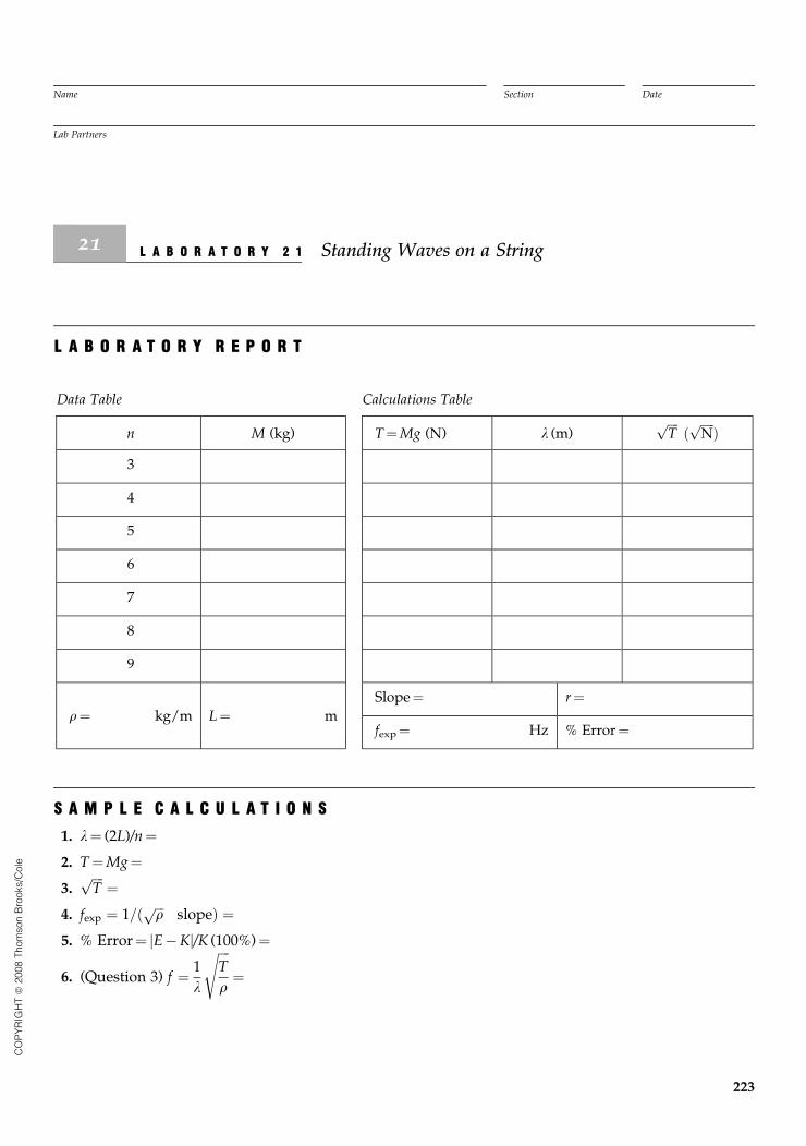
Name . . . . . . . . . . . . . . . . . . . . . . . . . . . . . . . . . . . . . . . . . . . . . . . . . . . . . . . . . . . . . . . . . . . . . . . . . Section . . . . . . . . . . . . . . . . Date . . . . . . . . . . . . . . . .
Lab Partners . . . . . . . . . . . . . . . . . . . . . . . . . . . . . . . . . . . . . . . . . . . . . . . . . . . . . . . . . . . . . . . . . . . . . . . . . . . . . . . . . . . . . . . . . . . . . . . . . . . . . . . . . . . . . . . . . . . .
21 L A B O R A T O R Y 2 1 Standing Waves on a String
L A B O R A T O R Y R E P O R T
S A M P L E C A L C U L A T I O N S1. l¼ (2L)/n¼2. T¼Mg¼3.
ffiffiffiffiT
p ¼4. fexp ¼ 1=ð ffiffiffi
rp
slopeÞ ¼5. % Error¼ jE�Kj/K (100%)¼
6. (Question 3) f ¼ 1
l
ffiffiffiffiT
r
s¼
COPYRIG
HTª
2008ThomsonBrooks/Cole
Data Table
n M (kg)
3
4
5
6
7
8
9
r¼ kg/m L¼ m
Calculations Table
T¼Mg (N) l (m)ffiffiffiffiT
p ð ffiffiffiffiffiN
p Þ
Slope¼ r¼
fexp¼ Hz % Error¼
223
Q U E S T I O N S1. What is the accuracy of your experimental value for the frequency? State clearly the basis for your
answer.
2. For the way in which the data were analyzed, the precision of the measurement would be related tothe uncertainty of the measured slope. Instead, use each measurement of T and l to calculate anindependent value for the frequency f. Calculate the seven values of the frequency using the equationf ¼ ð1=lÞ ffiffiffiffiffiffiffi
T=rp
. Calculate the mean and standard error of those seven values of the frequency and usethat to comment on the precision of the measurements of f.
3. Calculate the velocity for the n¼ 2 and for the n¼ 8 standing wave.
4. Calculate the tension T that would be required to produce the n¼ 1 standing wave in your string. Testa piece of the string with that much force and describe the results. In particular, does that much forcebreak the string?
5. Suppose that the string stretched significantly as the tension was increased. Howwould that affect thevalue of r for the string? Howwould that affect the results, andwould it cause an error in the directionof your observed experimental error?
224 Physics Laboratory Manual n Loyd

Speed of Sound—ResonanceTube
O B J E C T I V E So Determine the effective length of a closed tube at which resonance occurs for several tuning forks.
o Determine the wavelength of the standing wave from the effective length of the resonance tubefor each tuning fork.
o Determine the speed of sound from themeasuredwavelengths and known tuning fork frequenciesand compare with the accepted value.
E Q U I P M E N T L I S T. Resonance tubes (with length scale marked on the tube)
. Tuning forks (range 500 to 1040Hz) and rubber hammer
. Thermometer (one for the class)
T H E O R YTraveling waves of speed V, frequency f, and wavelength l are described by
V ¼ fl ðEq: 1Þ
We can determine the speed of a traveling wave for known frequency and wavelength from Equation 1.It is difficult to measure the properties of a traveling wave directly. When two waves of exactly the samespeed, frequency, and wavelength travel in opposite directions in the same region, they produce standingwaves. These standing waves can be measured easily.
This laboratory uses a device called a resonance tube to produce standing waves from the soundwaves emitted from a tuning fork. The can shown in Figure 22-1 contains water, and the level of the waterin the tube can be varied as the can is moved up and down. The water acts as the closed end of the tube,and changing the water level changes the effective length of the resonance tube.
A tuning fork, clamped just above the open end of the tube, is struck with a rubber hammer.Sound waves travel down the tube and are reflected when they strike the water. Standing waves areproduced by these traveling waves going in both directions inside the tube. The waves reflected from the
Physics Laboratory Manual n Loyd L A B O R A T O R Y 22
COPYRIG
HTª
2008ThomsonBrooks/Cole
225
ª 2008 Thomson Brooks/Cole, a part of TheThomson Corporation.Thomson, the Star logo, and Brooks/Cole are trademarks used herein under license. ALL RIGHTSRESERVED.No part of this workcovered by the copyright hereonmay be reproduced or used in any form or by any meansçgraphic, electronic, ormechanical, including photocopying, recording, taping,web distribution, informationstorage and retrieval systems,or in any othermannerçwithout the written permission of the publisher.
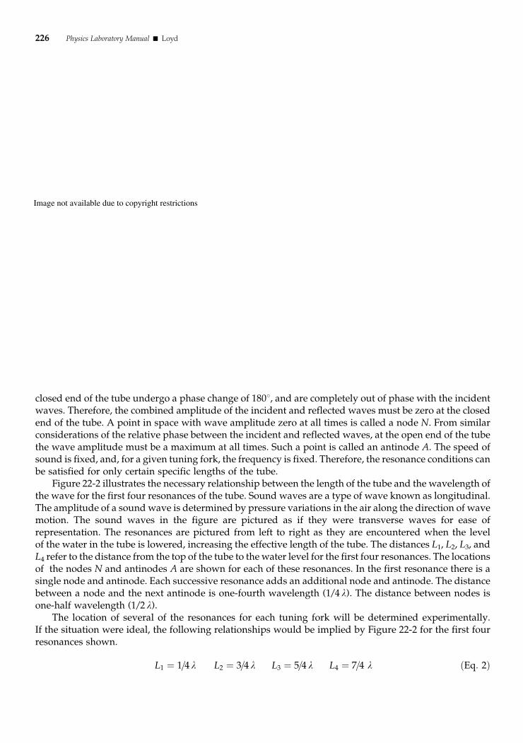
closed end of the tube undergo a phase change of 1808, and are completely out of phase with the incidentwaves. Therefore, the combined amplitude of the incident and reflected waves must be zero at the closedend of the tube. A point in space with wave amplitude zero at all times is called a node N. From similarconsiderations of the relative phase between the incident and reflected waves, at the open end of the tubethe wave amplitude must be a maximum at all times. Such a point is called an antinode A. The speed ofsound is fixed, and, for a given tuning fork, the frequency is fixed. Therefore, the resonance conditions canbe satisfied for only certain specific lengths of the tube.
Figure 22-2 illustrates the necessary relationship between the length of the tube and the wavelength ofthe wave for the first four resonances of the tube. Sound waves are a type of wave known as longitudinal.The amplitude of a soundwave is determined by pressure variations in the air along the direction of wavemotion. The sound waves in the figure are pictured as if they were transverse waves for ease ofrepresentation. The resonances are pictured from left to right as they are encountered when the levelof the water in the tube is lowered, increasing the effective length of the tube. The distances L1, L2, L3, andL4 refer to the distance from the top of the tube to the water level for the first four resonances. The locationsof the nodes N and antinodes A are shown for each of these resonances. In the first resonance there is asingle node and antinode. Each successive resonance adds an additional node and antinode. The distancebetween a node and the next antinode is one-fourth wavelength (1/4 l). The distance between nodes isone-half wavelength (1/2 l).
The location of several of the resonances for each tuning fork will be determined experimentally.If the situation were ideal, the following relationships would be implied by Figure 22-2 for the first fourresonances shown.
L1 ¼ 1=4 l L2 ¼ 3=4 l L3 ¼ 5=4 l L4 ¼ 7=4 l ðEq: 2Þ
226 Physics Laboratory Manual n Loyd
Image not available due to copyright restrictions
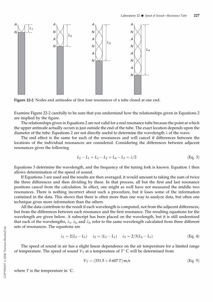
Examine Figure 22-2 carefully to be sure that you understand how the relationships given in Equations 2are implied by the figure.
The relationships given in Equations 2 are not valid for a real resonance tube because the point at whichthe upper antinode actually occurs is just outside the end of the tube. The exact location depends upon thediameter of the tube. Equations 2 are not directly useful to determine the wavelength l of the wave.
The end effect is the same for each of the resonances and will cancel if differences between thelocations of the individual resonances are considered. Considering the differences between adjacentresonances gives the following
L2 � L1 ¼ L3 � L2 ¼ L4 � L3 ¼ l=2 ðEq: 3Þ
Equations 3 determine the wavelength, and the frequency of the tuning fork is known. Equation 1 thenallows determination of the speed of sound.
If Equations 3 are used and the results are then averaged, it would amount to taking the sum of twicethe three differences and then dividing by three. In that process, all but the first and last resonancepositions cancel from the calculation. In effect, one might as well have not measured the middle tworesonances. There is nothing incorrect about such a procedure, but it loses some of the informationcontained in the data. This shows that there is often more than one way to analyze data, but often onetechnique gives more information than the others.
All the data contribute to the result if each wavelength is computed, not from the adjacent differences,but from the differences between each resonance and the first resonance. The resulting equations for thewavelength are given below. A subscript has been placed on the wavelength, but it is still understoodthat each of the wavelengths, l1, l2, and l3, refer to the same wavelength calculated from three differentsets of resonances. The equations are
l1 ¼ 2ðL2 � L1Þ l2 ¼ ðL3 � L1Þ l3 ¼ 2=3ðL4 � L1Þ ðEq: 4Þ
The speed of sound in air has a slight linear dependence on the air temperature for a limited rangeof temperature. The speed of sound VT at a temperature of T8 C will be determined from
VT ¼ ð331:5þ 0:607TÞm=s ðEq: 5Þ
where T is the temperature in 8C.
COPYRIG
HTª
2008ThomsonBrooks/Cole
L4
L3
L2
L1
A
N
A
N
A
N
A
N
A
N
A
N
A
N
A
N
A
N
A
N
Figure 22-2 Nodes and antinodes of first four resonances of a tube closed at one end.
Laboratory 22 n Speed of Sound—Resonance Tube 227
E X P E R I M E N T A L P R O C E D U R ENote carefully that tuning forks should be struck only with the rubber hammer. Take care to ensure that neither thehammer nor a vibrating tuning fork comes into contact with the tube.
1. Measure the room temperature of the air and record it in Data Table 1.
2. Adjust the water level until the can is essentially empty when the tube is almost full. The water levelin the tube should come to at least within 0.050m of the open end of the tube. It may be necessary toremove some water from the can when the water level is near the bottom of the tube.
3. Clamp a tuning fork above the top of the tube, and one partner should strike it repeatedly with therubber hammer. Keep the fork vibrating continuously with a large amplitude. With the tuningfork vibrating, another partner should slowly lower the water level from the top while listening for aresonance. The sound will be very loud when a resonance is achieved. Try to measure the position ofeach resonance to the nearest millimeter. Raise and lower the water level several times to producethree trials for the measured position of the first resonance and record the values in Data Table 2.Record the frequency of the tuning fork in Data Table 2.
4. Repeat the procedure in Step 3 to locate as many other resonances as possible. Depending upon thefrequency of the tuning fork, either three or four resonances should be attainable. Record in DataTable 2 the location of resonances that are attained.
5. Use a second tuning fork of different frequency and repeat Steps 1 through 4. Record in Data Table 3the frequency of the tuning fork and the position of as many resonances as are attained.
C A L C U L A T I O N S1. Use Equation 5 to calculate the accepted value of the speed of sound from the measured room
temperature. Record it in Data Table 1.
2. Calculate the mean and standard error of the three trials for the location of each of the resonances.Record each of the means and standard errors in Calculations Tables 2 and 3.
3. Use Equations 4 to calculate the wavelengths that are appropriate. If four resonances were found, thenall three values of l can be determined. If only the first three resonances were measured, then onlytwo values of l can be determined. If this is the case, just leave the Calculations Table blank at theappropriate position. Use the mean values of the lengths to calculate the wavelengths.
4. Calculate the mean and standard error for the number of independent wavelengthsmeasured for eachtuning fork. Record those values in the Calculations Tables as l and al.
5. From the values of l and the known values of the tuning fork frequencies, calculate the experimentalvalue for V, the speed of sound.
6. Calculate the percentage error of the experimental values of V compared to the accepted value of thespeed of sound in Data Table 1.
228 Physics Laboratory Manual n Loyd

Name . . . . . . . . . . . . . . . . . . . . . . . . . . . . . . . . . . . . . . . . . . . . . . . . . . . . . . . . . . . . . . . . . . . . . . . . . Section . . . . . . . . . . . . . . . . Date . . . . . . . . . . . . . . . .
22 L A B O R A T O R Y 2 2 Speed of Sound—Resonance Tube
P R E - L A B O R A T O R Y A S S I G N M E N T1. What is the equation that relates the speed V, the frequency f, and the wavelength l of a wave?
2. How are standing waves produced?
3. What name is given to a point in space where the wave amplitude is zero at all times?
4. What name is given to a point in space where the wave amplitude is a maximum at all times?
COPYRIG
HTª
2008ThomsonBrooks/Cole
229
5. What are the conditions that must be satisfied to produce a standing wave in a tube open at one endand closed at the other end?
6. For an ideal resonance tube an antinode occurs at the open end of the tube. What property of realresonance tubes slightly alters the position of this antinode?
7. A student using a tuning fork of frequency 512Hz observes that the speed of sound is 340m/s.What isthe wavelength of this sound wave? Show your work.
8. A student using a resonance tube determines that three resonances occur at distances of L1¼ 0.172m,L2¼ 0.529m, and L3¼ 0.884m below the open end of the tube. The frequency of the tuning fork used is480Hz. What is the average speed of sound from these data? Show your work.
230 Physics Laboratory Manual n Loyd
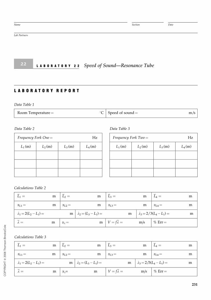
Name . . . . . . . . . . . . . . . . . . . . . . . . . . . . . . . . . . . . . . . . . . . . . . . . . . . . . . . . . . . . . . . . . . . . . . . . . Section . . . . . . . . . . . . . . . . Date . . . . . . . . . . . . . . . .
Lab Partners . . . . . . . . . . . . . . . . . . . . . . . . . . . . . . . . . . . . . . . . . . . . . . . . . . . . . . . . . . . . . . . . . . . . . . . . . . . . . . . . . . . . . . . . . . . . . . . . . . . . . . . . . . . . . . . . . . . .
22 L A B O R A T O R Y 2 2 Speed of Sound—Resonance Tube
L A B O R A T O R Y R E P O R T
COPYRIG
HTª
2008ThomsonBrooks/Cole
Data Table 1
Room Temperature¼ 8C Speed of sound¼ m/s
Data Table 2
Frequency Fork One¼ Hz
L1 (m) L2 (m) L3 (m) L4 (m)
Data Table 3
Frequency Fork Two¼ Hz
L1 (m) L2 (m) L3 (m) L4 (m)
Calculations Table 2
L1 ¼ m L2 ¼ m L3 ¼ m L4 ¼ m
aL1¼ m aL2¼ m aL3¼ m aL4¼ m
l1¼ 2(L2� L1)¼ m l2¼ (L3� L1)¼ m l3¼ 2/3(L4� L1)¼ m
l ¼ m al¼ m V ¼ fl ¼ m=s % Err¼
Calculations Table 3
L1 ¼ m L2 ¼ m L3 ¼ m L4 ¼ m
aL1¼ m aL2¼ m aL3¼ m aL4¼ m
l1¼ 2(L2� L1)¼ m l2¼ (L3� L1)¼ m l3¼ 2/3(L4� L1)¼ m
l ¼ m al= m V ¼ fl ¼ m=s % Err¼
231
S A M P L E C A L C U L A T I O N S1. Speed Sound¼ 331.5þ 0.607 T¼2. l1¼ 2(L2� L1)¼3. l2¼ (L3�L1)¼4. l3¼ 2/3(L4� L1)¼5. V ¼ fl ¼6. % Error¼ jE�Kj/K (100%)¼
Q U E S T I O N S1. What is the accuracy of each of your measurements of the speed of sound? State clearly the evidence
for your answer.
2. What is the precision of each of your measurements of the speed of sound? State clearly the evidencefor your answer.
3. Equations 2 provide a means to determine the end correction for the tube. Using the value of lfor the first tuning fork, calculate values for L1 and L2 from those equations. They should be largerthan the measured values of L1 and L2 by an amount equal to the end correction. Repeat thecalculation for the second tuning fork. Compare these values for the end correction and comment onthe consistency of the results.
232 Physics Laboratory Manual n Loyd
4. Suppose that the temperature had been 10 8C higher than the value measured for the room tempe-rature. How much would that have changed the measured value of L2� L1 for each tuning fork?Would L2� L1 be larger or smaller at this higher temperature?
5. Draw a figure showing the fifth resonance in a tube closed at one end. Show also how the length ofthe tube L5 is related to the wavelength l.
COPYRIG
HTª
2008ThomsonBrooks/Cole
Laboratory 22 n Speed of Sound—Resonance Tube 233

This page intentionally left blank

Specific Heat of Metals
O B J E C T I V E So Demonstrate the heat exchange within a calorimeter.
o Determine the specific heat of two samples of different metals.
E Q U I P M E N T L I S T. Calorimeter and stirrer, steam generator, Bunsen burner, or electric heating plate
. Metal shot (two different kinds of metal)
. Two thermometers (preferably one 0–1008C and the other 0–508C) and glycerin
T H E O R YTwo objects at different temperatures, placed in thermal contact with each other, exchange thermal energyuntil they are in thermal equilibrium at the same temperature. The exchanged thermal energy is knownas heat. The temperature change that each object experiences is determined by the mass and specific heatof each object. The specific heat c is the amount of heat per unit mass required to change the temperatureby one degree. The units used in this laboratory for specific heat are cal/g–C8. The heat or thermal energychange for any object in the system can be written as
Heat ¼ Thermal energy change ¼ McDT ðEq: 1Þ
where M is mass in grams, c is specific heat in cal/g–C8, and DT is the temperature change in C8. Theunits of the thermal energy change or heat will be calories. In an ideal experimental arrangement designedto investigate this concept, all exchanges of heat are among the objects of the system. In real systems, heatlosses from the system or gains into the system are held to aminimum. A device that produces a thermallyisolated environment to maximize heat exchanges inside the system is called a calorimeter. The calo-rimeter used in this laboratory consists of two metal cups held apart by a plastic ring that produces aninsulating air space between the cups. The cups also have an insulating plastic top that contains a hole intowhich the stirrer is placed, and a rubber stopper with a hole into which a thermometer is placed. A pictureof a calorimeter is shown in Figure 23-1.
Metal shot will be heated to the temperature of steam in a steam generator and then placed into acalorimeter containing water near room temperature. The metal shot will lose heat, and that heat will begained by the water, the calorimeter cup, and the stirrer in the calorimeter. The stirrer is used to mix the
Physics Laboratory Manual n Loyd L A B O R A T O R Y 23
COPYRIG
HTª
2008ThomsonBrooks/Cole
235
ª 2008 Thomson Brooks/Cole, a part of TheThomson Corporation.Thomson, the Star logo, and Brooks/Cole are trademarks used herein under license. ALL RIGHTSRESERVED.No part of this workcovered by the copyright hereonmay be reproduced or used in any form or by any meansçgraphic, electronic, ormechanical, including photocopying, recording, taping,web distribution, informationstorage and retrieval systems,or in any othermannerçwithout the written permission of the publisher.
system to ensure that all parts of the system quickly come to thermal equilibrium. In equation form, thestatement that the heat lost by the metal shot equals the heat gained by the other parts of the system is
MmcmðTm � TeÞ ¼ MwcwðTe � ToÞ þMcalccalðTe � ToÞ þMscsðTe � ToÞ ðEq: 2Þ
where theM’s are masses and the c’s are specific heats. The subscripts are m for metal, w for water, cal forcalorimeter, and s for stirrer. The initial temperature of themetal shot is Tm, the original temperature of thewater, cup, and stirrer is To, and the final equilibrium temperature of the system is Te.
E X P E R I M E N T A L P R O C E D U R E1. Place about 250 g of one kind of metal shot into the cup that is designed to fit into the steam generator.
2. Fill the steam generator about one-half full of water. Keep the water level below the bottom of the cupthat is placed in the generator. The cup should be heated by steam from the water. Use whatevermeans of heating is provided (Bunsen burner or electric heating plate) to heat the generator.
3. Place a thermometer that reads 0–1008C into the metal shot. If the thermometer is a mercury ther-mometer, be very careful not to break the bulb as you work it down into the shot. Place paper or someother insulation around the top of the cup to keep the outside air from cooling the top layer of shot.
4. While the shot is heating, determine the mass of the inner calorimeter cup and the stirrer separatelyand record their mass in the Data Table. Obtain from your instructor the values for ccal and cs, thespecific heats of the calorimeter cup and the stirrer, and record them in the Data Table.
5. Place about 100 g of water in the inner calorimeter cup and determine the combined mass of the cup,stirrer, and water. Determine the mass of the water by subtraction and record it in the Data Table. Theinitial temperature of the water should ideally be a few degrees below the room temperature. This willtend to compensate for interaction with the air.
6. Assemble the calorimeter, placing the second thermometer in the rubber stopper. Use glycerin on thethermometer so that it may be easily slipped into the hole in the stopper. If using a glass thermometer,be extremely careful. If the thermometer breaks, you can cut yourself severely. Stir the water slowly to be surethat all parts of the system are in equilibrium. Record the temperature of the water, calorimeter, andstirrer as To in the Data Table. Take this reading for To just prior to performing Step 8 below.
236 Physics Laboratory Manual n Loyd
Image not available due to copyright restrictions
7. Take the temperature of the metal shot every few minutes. Move the bulb around carefully in the shotto be sure all parts are in equilibrium. The temperature should rise and then level off at essentially theboiling point of water. This will probably be a few degrees below 1008C depending upon the localelevation above sea level. Record the value (to the nearest 0.18) of the maximum temperature as Tm inthe Data Table.
8. Remove the thermometer from the shot and quickly transfer the shot to thewater in the inner calorimetercup. It is very important not to splash water out of the cup in this process. This can easily happen whenremoving the insulating plastic cover or when placing the shot in the water.
9. Place the insulating cover back on the calorimeter and slowly stir the water while watching the ther-mometer in the calorimeter.When themaximum temperature is reached, record its value (to the nearest0.18) as the equilibrium temperature Te.
10. Remove the inner calorimeter cup and determine the mass of the cup, stirrer, water, and metal shot.Record that value in the Data Table. Determine the mass of the shot used by subtraction and recordthat value in the Data Table.
11. Discard the water but do not lose any of the shot. Place the wet shot on paper towels, spread it out, andallow the shot to dry. Before leaving the laboratory andwhen the shot is completely dry, return it to itsproper container. Be careful not to mix the two kinds of metal shot.
12. From Appendix II, determine the known value of the specific heat for the type of metal of the shot andrecord it in the Data Table.
13. Repeat all of the above procedure for a second type of metal shot.
C A L C U L A T I O N S1. In Equation 2 all of the variables are known except for the specific heat of the metal shot. Solve
Equation 2 for the specific heat of the metal shot and record that value as the experimental value in theCalculations Table.
2. Calculate the percentage error between your experimental value and the known value of the specificheat for each type of metal.
COPYRIG
HTª
2008ThomsonBrooks/Cole
Laboratory 23 n Specific Heat of Metals 237

This page intentionally left blank
Name . . . . . . . . . . . . . . . . . . . . . . . . . . . . . . . . . . . . . . . . . . . . . . . . . . . . . . . . . . . . . . . . . . . . . . . . . Section . . . . . . . . . . . . . . . . Date . . . . . . . . . . . . . . . .
23 L A B O R A T O R Y 2 3 Specific Heat of Metals
P R E - L A B O R A T O R Y A S S I G N M E N T1. What is the definition of specific heat?
2. What is the name for a device that provides a thermally isolated environment in which substancesexchange heat?
A heated piece of metal at a temperature T1 is placed into a calorimeter containing water and a stirrer.The temperature of the calorimeter, water, and stirrer is initially T2 where T1 >T2. The system is stirredcontinuously until it comes to equilibrium at a temperature of T3. Answer Questions 3–5 concerningwhat happens.
3. The final equilibrium temperature of the system is such that
(a) T3 >T1 >T2 (b) T1 <T2 <T3 (c) T1 <T3 <T2 (d) T1 >T3 >T2
4. The heat lost by the metal DQm and the heat gained by the calorimeter system DQc obey which of thefollowing relationships?
(a) DQm>DQc (b) DQm<DQc (c) DQm¼DQc
COPYRIG
HTª
2008ThomsonBrooks/Cole
239

5. What is the purpose of stirring the system continuously?
6. A 350 g piece of metal is at an initial temperature of 22.08C. It absorbs 1000 cal of thermal energy, andits final temperature is 45.08C. What is the specific heat of the metal? Show your work.
7. A 250.0 g sample of metal shot is heated to a temperature of 98.08C. It is placed in 100.0 g of water in abrass calorimeter cup with a brass stirrer. The total mass of the cup and the stirrer is 50.0 g. The initialtemperature of the water, stirrer, and calorimeter cup is 20.08C. The final equilibrium temperatureof the system is 30.08C. What is the specific heat of the metal sample? (The specific heat of brass is0.092 cal/g–C8.) Show your work.
240 Physics Laboratory Manual n Loyd

Name . . . . . . . . . . . . . . . . . . . . . . . . . . . . . . . . . . . . . . . . . . . . . . . . . . . . . . . . . . . . . . . . . . . . . . . . . Section . . . . . . . . . . . . . . . . Date . . . . . . . . . . . . . . . .
Lab Partners . . . . . . . . . . . . . . . . . . . . . . . . . . . . . . . . . . . . . . . . . . . . . . . . . . . . . . . . . . . . . . . . . . . . . . . . . . . . . . . . . . . . . . . . . . . . . . . . . . . . . . . . . . . . . . . . . . . .
23 L A B O R A T O R Y 2 3 Specific Heat of Metals
L A B O R A T O R Y R E P O R T
Data Table
Mass Cup¼ g Mass Stirrer¼ g
MetalCupþH2Oþ Stirrer
Cupþ StirrerþH2Oþ Shot H2O Shot To Tm Te
g g g g 8C 8C 8C
g g g g 8C 8C 8C
Calculations Table
Metal Known Specific Heat Measured Specific Heat Percentage Error
Cal/g–C8 Cal/g–C8
Cal/g–C8 Cal/g–C8
S A M P L E C A L C U L A T I O N S1. MWater¼MCupþ StirrerþWater�Mcup�Mstirrer¼2. Mshot¼Mcupþ stirrerþwaterþ shot�Mcupþ stirrerþwater¼3. cm¼ [Mwcw(Te�To)þMccc(Te�To)þMscs(Te�To)]/Mm(Tm�Te)]
4. % Error¼ (jE�Kj/K)(100%)¼
COPYRIG
HTª
2008ThomsonBrooks/Cole
241

Q U E S T I O N S1. What is the accuracy of your results for the specific heats of themetals? Can you suggest any change in
the original temperature of the metal that would improve the results?
2. Can youmake a quantitative statement about the precision of your results? If you canmake a statementabout the precision, do so. If you cannot make any statement about the precision, suggest whatmeasurements would allow you to do so.
3. Suppose the shot were wet and thus included some water at the same temperature as the shot whenit was placed in the calorimeter. How would this affect the results?
4. What would the change in temperature of the water have been if 200 g of water had been used witheach of the samples?Would this have tended to improve the results, tended tomake the results worse,or tended to have no effect on the results?
242 Physics Laboratory Manual n Loyd

Linear Thermal Expansion
O B J E C T I V E So Demonstrate that for the same temperature change the thermal expansion depends upon the
type of metal.
o Determine the value of the linear coefficient of thermal expansion a for several metals andcompare the results to known values.
E Q U I P M E N T L I S T. Linear expansion apparatus consisting of steam jacket containing a metal rod
. Steam generator, rubber tubing, and beaker to catch steam condensation
. Bunsen burner and stand, or electric heating plate
. Meter stick, thermometer (0–1008C)
. Ohmmeter if using micrometer screw-type indicator
T H E O R YMost materials expand as their temperature increases. The expansion depends not upon the heat input,but rather upon the temperature change. Temperature expansion occurs in three dimensions, but we willinvestigate only one dimensional change in the length of a rod.
A metal rod of some initial length Lo at some initial temperature To is heated to some temperature T1.The length of the rod will increase to a new length L1. The change in length of the rod DL¼ L1� Lo is foundto be proportional to the original length of the rod Lo and to the change in the temperature DT whereDT¼T1�To. In equation form the result is
DL ¼ aLo DT ðEq: 1Þ
where a is a constant called the linear coefficient of thermal expansion. Solving Equation 1 for theconstant a gives
a ¼ DLLoDT
¼ L1 � LoLoDT
ðEq: 2Þ
From Equation 2 it is clear that a is the fractional change in length per unit change in the temperature.Because the fractional change in length DL/Lo has no dimensions, the units of a are (C8)�1. Strictly
Physics Laboratory Manual n Loyd L A B O R A T O R Y 24
COPYRIG
HTª
2008ThomsonBrooks/Cole
243
ª 2008 Thomson Brooks/Cole, a part of TheThomson Corporation.Thomson, the Star logo, and Brooks/Cole are trademarks used herein under license. ALL RIGHTSRESERVED.No part of this workcovered by the copyright hereonmay be reproduced or used in any form or by any meansçgraphic, electronic, ormechanical, including photocopying, recording, taping,web distribution, informationstorage and retrieval systems,or in any othermannerçwithout the written permission of the publisher.
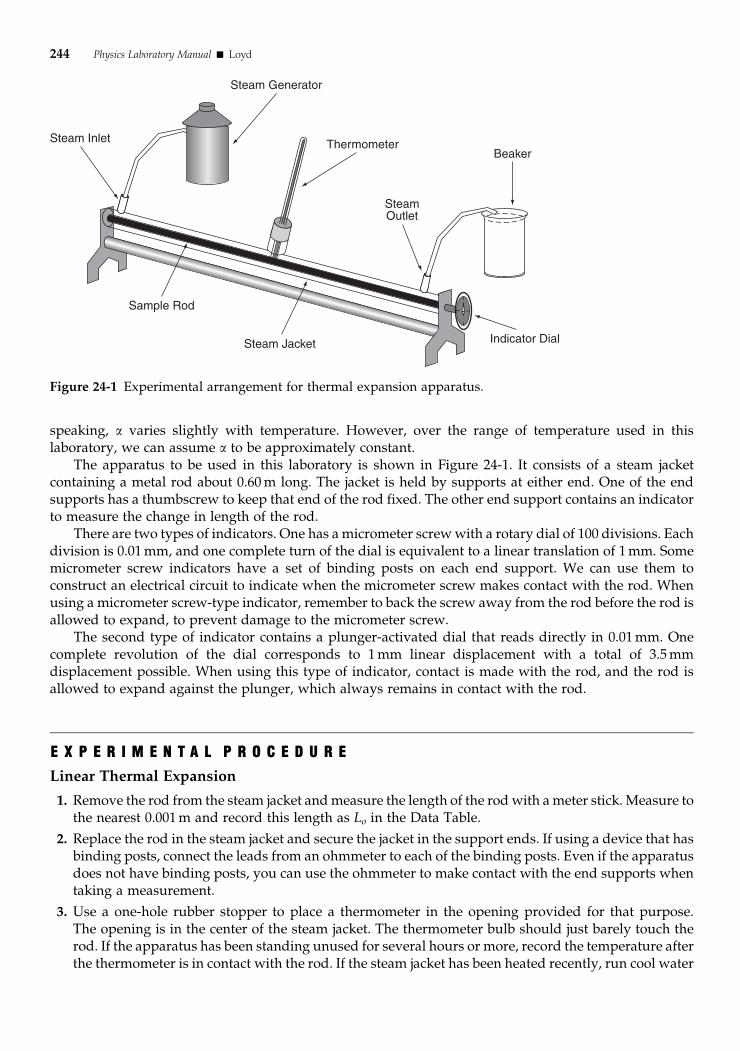
speaking, a varies slightly with temperature. However, over the range of temperature used in thislaboratory, we can assume a to be approximately constant.
The apparatus to be used in this laboratory is shown in Figure 24-1. It consists of a steam jacketcontaining a metal rod about 0.60m long. The jacket is held by supports at either end. One of the endsupports has a thumbscrew to keep that end of the rod fixed. The other end support contains an indicatorto measure the change in length of the rod.
There are two types of indicators. One has amicrometer screwwith a rotary dial of 100 divisions. Eachdivision is 0.01mm, and one complete turn of the dial is equivalent to a linear translation of 1mm. Somemicrometer screw indicators have a set of binding posts on each end support. We can use them toconstruct an electrical circuit to indicate when the micrometer screw makes contact with the rod. Whenusing a micrometer screw-type indicator, remember to back the screw away from the rod before the rod isallowed to expand, to prevent damage to the micrometer screw.
The second type of indicator contains a plunger-activated dial that reads directly in 0.01mm. Onecomplete revolution of the dial corresponds to 1mm linear displacement with a total of 3.5mmdisplacement possible. When using this type of indicator, contact is made with the rod, and the rod isallowed to expand against the plunger, which always remains in contact with the rod.
E X P E R I M E N T A L P R O C E D U R ELinear Thermal Expansion
1. Remove the rod from the steam jacket andmeasure the length of the rodwith ameter stick. Measure tothe nearest 0.001m and record this length as Lo in the Data Table.
2. Replace the rod in the steam jacket and secure the jacket in the support ends. If using a device that hasbinding posts, connect the leads from an ohmmeter to each of the binding posts. Even if the apparatusdoes not have binding posts, you can use the ohmmeter to make contact with the end supports whentaking a measurement.
3. Use a one-hole rubber stopper to place a thermometer in the opening provided for that purpose.The opening is in the center of the steam jacket. The thermometer bulb should just barely touch therod. If the apparatus has been standing unused for several hours or more, record the temperature afterthe thermometer is in contact with the rod. If the steam jacket has been heated recently, run cool water
Steam Generator
SteamOutlet
BeakerSteam Inlet Thermometer
Indicator DialSteam Jacket
Sample Rod
Figure 24-1 Experimental arrangement for thermal expansion apparatus.
244 Physics Laboratory Manual n Loyd
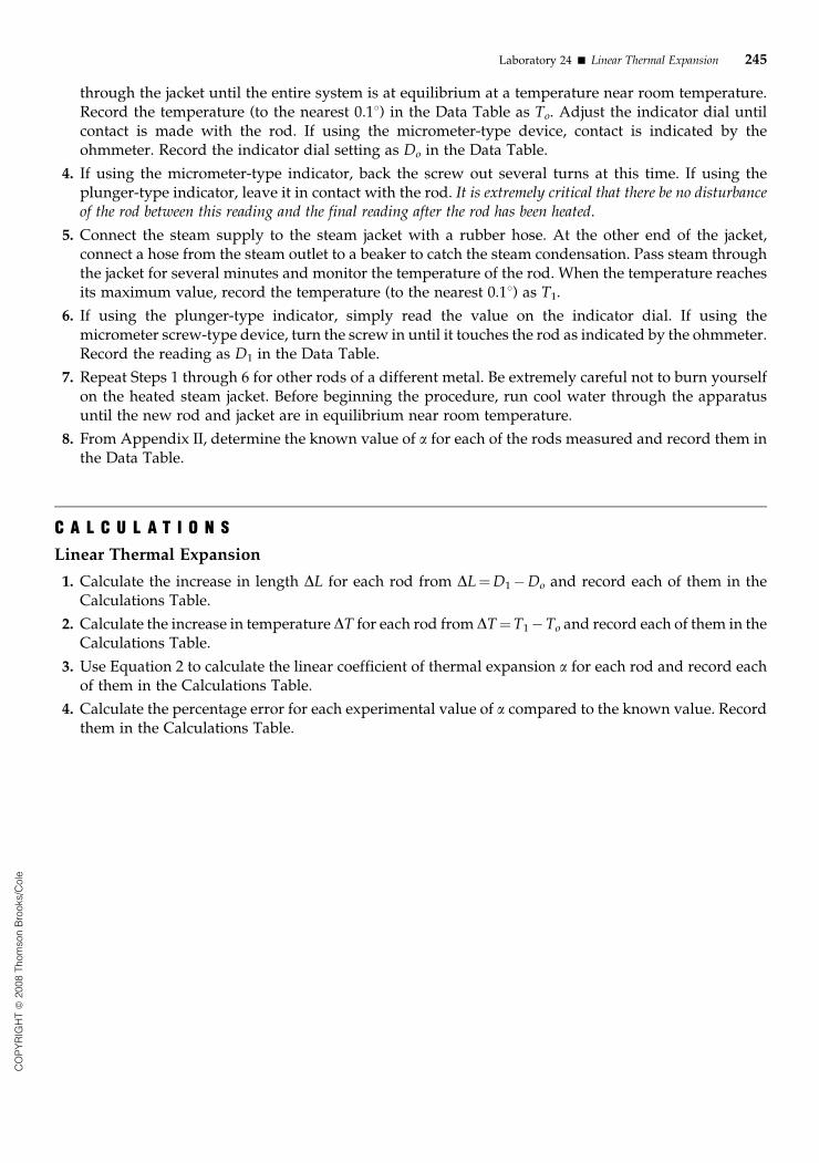
through the jacket until the entire system is at equilibrium at a temperature near room temperature.Record the temperature (to the nearest 0.18) in the Data Table as To. Adjust the indicator dial untilcontact is made with the rod. If using the micrometer-type device, contact is indicated by theohmmeter. Record the indicator dial setting as Do in the Data Table.
4. If using the micrometer-type indicator, back the screw out several turns at this time. If using theplunger-type indicator, leave it in contact with the rod. It is extremely critical that there be no disturbanceof the rod between this reading and the final reading after the rod has been heated.
5. Connect the steam supply to the steam jacket with a rubber hose. At the other end of the jacket,connect a hose from the steam outlet to a beaker to catch the steam condensation. Pass steam throughthe jacket for several minutes and monitor the temperature of the rod. When the temperature reachesits maximum value, record the temperature (to the nearest 0.18) as T1.
6. If using the plunger-type indicator, simply read the value on the indicator dial. If using themicrometer screw-type device, turn the screw in until it touches the rod as indicated by the ohmmeter.Record the reading as D1 in the Data Table.
7. Repeat Steps 1 through 6 for other rods of a different metal. Be extremely careful not to burn yourselfon the heated steam jacket. Before beginning the procedure, run cool water through the apparatusuntil the new rod and jacket are in equilibrium near room temperature.
8. From Appendix II, determine the known value of a for each of the rods measured and record them inthe Data Table.
C A L C U L A T I O N SLinear Thermal Expansion
1. Calculate the increase in length DL for each rod from DL¼D1�Do and record each of them in theCalculations Table.
2. Calculate the increase in temperature DT for each rod from DT¼T1�To and record each of them in theCalculations Table.
3. Use Equation 2 to calculate the linear coefficient of thermal expansion a for each rod and record eachof them in the Calculations Table.
4. Calculate the percentage error for each experimental value of a compared to the known value. Recordthem in the Calculations Table.
COPYRIG
HTª
2008ThomsonBrooks/Cole
Laboratory 24 n Linear Thermal Expansion 245

This page intentionally left blank

Name . . . . . . . . . . . . . . . . . . . . . . . . . . . . . . . . . . . . . . . . . . . . . . . . . . . . . . . . . . . . . . . . . . . . . . . . . Section . . . . . . . . . . . . . . . . Date . . . . . . . . . . . . . . . .
24 L A B O R A T O R Y 2 4 Linear Thermal Expansion
P R E - L A B O R A T O R Y A S S I G N M E N T1. An object undergoes a change in length DL because of a change in its temperature. What are the three
factors on which this change in length depends?
2. What are the units for the linear thermal coefficient of expansion a?
3. Most materials expand when the temperature is raised. What can you conclude about a for a materialthat contracts when its temperature is raised?
4. A copper rod has a length of 1.117m when its temperature is 22.08C. If the temperature of the rod israised to 275.08C, what is the new length of the rod? [The value of a for copper is 16.8� 10�6 (C8)�1.]Show your work.
COPYRIG
HTª
2008ThomsonBrooks/Cole
247

5. Iron rails are used to build a railroad track. If each rail is 10.000m long when it is placed in the track ata temperature of 20.08C, how much space must be left between the rails so that they just touch eachother when the temperature is 40.08C? [The value of a for iron is 11.4� 10 (C8)�1.] Show your work.
6. A rod in a steam jacket is measured to have a length of 0.600m at a temperature of 22.08C. Steam isthen passed through the jacket for several minutes until the rod is at a temperature of 98.08C.The increase in the length of the rod is measured by a micrometer screw arrangement to be 1.19mm.What is the linear thermal coefficient of expansion a for the rod? Show your work.
7. Considering the value of a found for the rod in Question 6, from what kind of metal is it probablymade?
248 Physics Laboratory Manual n Loyd

Name . . . . . . . . . . . . . . . . . . . . . . . . . . . . . . . . . . . . . . . . . . . . . . . . . . . . . . . . . . . . . . . . . . . . . . . . . Section . . . . . . . . . . . . . . . . Date . . . . . . . . . . . . . . . .
Lab Partners . . . . . . . . . . . . . . . . . . . . . . . . . . . . . . . . . . . . . . . . . . . . . . . . . . . . . . . . . . . . . . . . . . . . . . . . . . . . . . . . . . . . . . . . . . . . . . . . . . . . . . . . . . . . . . . . . . . .
24 L A B O R A T O R Y 2 4 Linear Thermal Expansion
L A B O R A T O R Y R E P O R T
S A M P L E C A L C U L A T I O N S1. DL¼D1�Do¼2. DT¼T1�To¼3. a ¼ DL
LoDT¼
4. jE�Kj/K (100%)¼
COPYRIG
HTª
2008ThomsonBrooks/Cole
Data Table
Metal Known a (C8)�1 Lo (m) To (8C) T1 (8C) Do (m) D1 (m)
Calculations Table
Metal DL (m) DT (C8) aexp (C8)�1 % Error
249
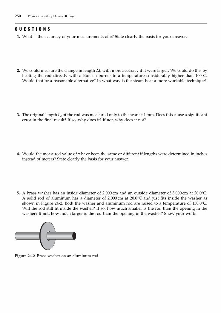
Q U E S T I O N S1. What is the accuracy of your measurements of a? State clearly the basis for your answer.
2. We could measure the change in length DL with more accuracy if it were larger. We could do this byheating the rod directly with a Bunsen burner to a temperature considerably higher than 1008C.Would that be a reasonable alternative? In what way is the steam heat a more workable technique?
3. The original length Lo of the rod was measured only to the nearest 1mm. Does this cause a significanterror in the final result? If so, why does it? If not, why does it not?
4. Would the measured value of a have been the same or different if lengths were determined in inchesinstead of meters? State clearly the basis for your answer.
5. A brass washer has an inside diameter of 2.000 cm and an outside diameter of 3.000 cm at 20.08C.A solid rod of aluminum has a diameter of 2.000 cm at 20.08C and just fits inside the washer asshown in Figure 24-2. Both the washer and aluminum rod are raised to a temperature of 150.08C.Will the rod still fit inside the washer? If so, how much smaller is the rod than the opening in thewasher? If not, how much larger is the rod than the opening in the washer? Show your work.
Figure 24-2 Brass washer on an aluminum rod.
250 Physics Laboratory Manual n Loyd

The Ideal Gas Law
O B J E C T I V E So Demonstrate that the pressure P of a gas at a fixed temperature is proportional to the quantity
(1/V) where V is the gas volume.
o Demonstrate that the volume V of a gas at a fixed pressure is proportional to the temperature Tof the gas.
o Determineanexperimentalvalue for the constant that relatesCelsius temperatureTC to theabsolutetemperature T and compare the experimental value for this constant with its known value of273.15.
E Q U I P M E N T L I S T. Gas law apparatus, Vaseline or stopcock grease, and string
. Thermometer (0–1008C) and vernier calipers
. 600mL beaker and tongs to fit the beaker
. Masses to allow application of up to 6 kg in 1 kg increments
. Electric heating plate or Bunsen burner (If a Bunsen burner is used, a stand to hold beaker while it isheated is also needed.)
. One large container of ice for the class
T H E O R YConsider a gas containing Nmolecules confined to a volume V, at a pressure P, and temperature T. In themost general case, all of these quantities vary over awide range, and the equation of state that relates them isvery complex. If only gases at low density are considered, the equation of state is greatly simplified. A gasthat satisfies these conditions is referred to as an ideal gas. Although there are no true ideal gases, most realgases approximate an ideal gas near room temperature and atmospheric pressure. The ideal gas law is
PV ¼ NkBT ðEq: 1Þ
The SI units of pressure P are N/m2, and the SI units of volumeV are m3. The constant kB¼ 1.38� 10�23 J/Kis called Boltzmann’s constant. In Equation 1 the Kelvin temperature scale must be used. The relationshipbetween temperature in Celsius TC and the Kelvin temperature T is
Physics Laboratory Manual n Loyd L A B O R A T O R Y 25
COPYRIG
HTª
2008ThomsonBrooks/Cole
251
ª 2008 Thomson Brooks/Cole, a part of TheThomson Corporation.Thomson, the Star logo, and Brooks/Cole are trademarks used herein under license. ALL RIGHTSRESERVED.No part of this workcovered by the copyright hereonmay be reproduced or used in any form or by any meansçgraphic, electronic, ormechanical, including photocopying, recording, taping,web distribution, informationstorage and retrieval systems,or in any othermannerçwithout the written permission of the publisher.
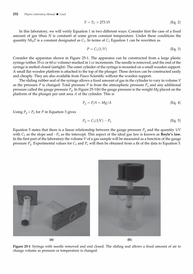
T ¼ TC þ 273:15 ðEq: 2Þ
In this laboratory, we will verify Equation 1 in two different ways. Consider first the case of a fixedamount of gas (thus N is constant) at some given constant temperature. Under these conditions thequantity NkBT is a constant designated as C1. In terms of C1 Equation 1 can be rewritten as
P ¼ C1ð1=VÞ ðEq: 3Þ
Consider the apparatus shown in Figure 25-1. The apparatus can be constructed from a large plasticsyringe (either 35 cc or 60 cc volume) marked in 1 cc increments. The needle is removed, and the end of thesyringe is melted closed (airtight). The outer cylinder of the syringe is mounted on a small wooden support.A small flat wooden platform is attached to the top of the plunger. These devices can be constructed easilyand cheaply. They are also available from Pasco Scientific without the wooden support.
The sliding rubber seal of the syringe allows a fixed amount of gas in the cylinder to vary in volume Vas the pressure P is changed. Total pressure P is from the atmospheric pressure Pa and any additionalpressure called the gauge pressure Pg. In Figure 25-1(b) the gauge pressure is the weightMg placed on theplatform of the plunger per unit area A of the cylinder. This is
Pg ¼ F=A ¼ Mg=A ðEq: 4Þ
Using PgþPa for P in Equation 3 gives
Pg ¼ C1ð1=VÞ � Pa ðEq: 5Þ
Equation 5 states that there is a linear relationship between the gauge pressure Pg and the quantity 1/Vwith C1 as the slope and�Pa as the intercept. This aspect of the ideal gas law is known as Boyle’s law.In the first part of the laboratory the volume V of a gas sample will be measured as a function of the gaugepressure Pg. Experimental values for C1 and Pa will then be obtained from a fit of the data to Equation 5.
(a) (b)
Figure 25-1 Syringe with needle removed and end closed. The sliding seal allows a fixed amount of air tochange volume as pressure or temperature is changed.
252 Physics Laboratory Manual n Loyd
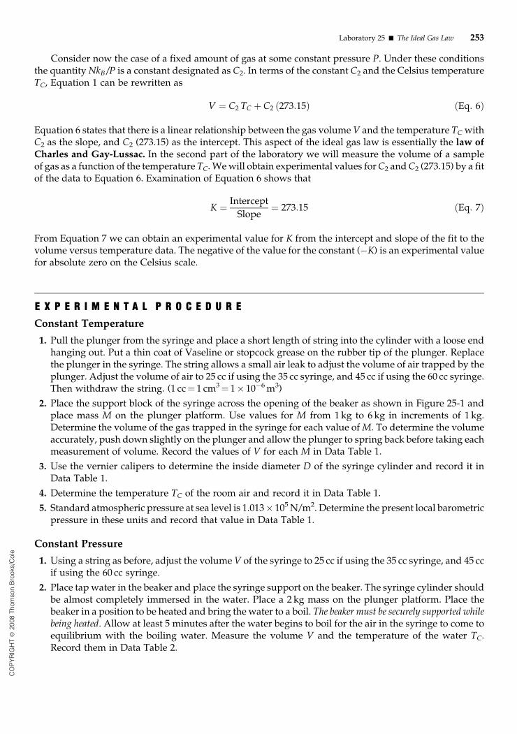
Consider now the case of a fixed amount of gas at some constant pressure P. Under these conditionsthe quantityNkB/P is a constant designated as C2. In terms of the constant C2 and the Celsius temperatureTC, Equation 1 can be rewritten as
V ¼ C2 TC þ C2 ð273:15Þ ðEq: 6Þ
Equation 6 states that there is a linear relationship between the gas volume V and the temperature TCwithC2 as the slope, and C2 (273.15) as the intercept. This aspect of the ideal gas law is essentially the law ofCharles and Gay-Lussac. In the second part of the laboratory we will measure the volume of a sampleof gas as a function of the temperature TC. Wewill obtain experimental values forC2 andC2 (273.15) by a fitof the data to Equation 6. Examination of Equation 6 shows that
K ¼ Intercept
Slope¼ 273:15 ðEq: 7Þ
From Equation 7 we can obtain an experimental value for K from the intercept and slope of the fit to thevolume versus temperature data. The negative of the value for the constant (�K) is an experimental valuefor absolute zero on the Celsius scale.
E X P E R I M E N T A L P R O C E D U R EConstant Temperature
1. Pull the plunger from the syringe and place a short length of string into the cylinder with a loose endhanging out. Put a thin coat of Vaseline or stopcock grease on the rubber tip of the plunger. Replacethe plunger in the syringe. The string allows a small air leak to adjust the volume of air trapped by theplunger. Adjust the volume of air to 25 cc if using the 35 cc syringe, and 45 cc if using the 60 cc syringe.Then withdraw the string. (1 cc¼ 1 cm3¼ 1� 10�6m3)
2. Place the support block of the syringe across the opening of the beaker as shown in Figure 25-1 andplace mass M on the plunger platform. Use values for M from 1kg to 6 kg in increments of 1 kg.Determine the volume of the gas trapped in the syringe for each value ofM. To determine the volumeaccurately, push down slightly on the plunger and allow the plunger to spring back before taking eachmeasurement of volume. Record the values of V for each M in Data Table 1.
3. Use the vernier calipers to determine the inside diameter D of the syringe cylinder and record it inData Table 1.
4. Determine the temperature TC of the room air and record it in Data Table 1.
5. Standard atmospheric pressure at sea level is 1.013� 105 N/m2. Determine the present local barometricpressure in these units and record that value in Data Table 1.
Constant Pressure
1. Using a string as before, adjust the volume V of the syringe to 25 cc if using the 35 cc syringe, and 45 ccif using the 60 cc syringe.
2. Place tap water in the beaker and place the syringe support on the beaker. The syringe cylinder shouldbe almost completely immersed in the water. Place a 2 kg mass on the plunger platform. Place thebeaker in a position to be heated and bring the water to a boil. The beaker must be securely supported whilebeing heated. Allow at least 5 minutes after the water begins to boil for the air in the syringe to come toequilibrium with the boiling water. Measure the volume V and the temperature of the water TC.Record them in Data Table 2.
COPYRIG
HTª
2008ThomsonBrooks/Cole
Laboratory 25 n The Ideal Gas Law 253

3. Remove the 2 kg mass from the plunger. Use the beaker tongs to carefully remove the beaker from thesource of heat and set it on the laboratory table. Replace the 2 kgmass on the plunger. Add small piecesof ice to the water and stir the mixture after each addition of ice until all the ice melts. Monitor thetemperature of the water at all times. Determine the volumeV of the syringe for water temperatures ofabout 758C, 508C, and 258C. For each temperature at which the volume is determined, there should beno ice in thewater when the volume ismeasured. Allow a fewminutes at each temperature to establishequilibrium between thewater and the air in the syringe. Record the volumeV and the temperature TC
(to the nearest 0.18C) in Data Table 2.
4. For the final temperature add enough ice until ice and water are at equilibrium near 08C. Some watermay have to be discarded. Allow at least five minutes for the air in the syringe to come to equilibriumwith the ice and water and record the volume V of the trapped air and the temperature TC (to thenearest 0.18C) in Data Table 2.
C A L C U L A T I O N SConstant Temperature
1. Calculate the cross-sectional area A of the syringe from the measured diameter D of the cylinderwhere A¼ pD2/4 and record in Calculations Table 1.
2. Calculate the force F¼Mg with g¼ 9.80m/s2 for each mass M and record in Calculations Table 1.
3. Use Equation 4 to calculate gauge pressure Pg for each value of F and record in Calculations Table 1.
4. For each value of V calculate the quantity 1/V and record in Calculations Table 1.
5. Perform a linear least squares fit with Pg as the vertical axis and 1/V as the horizontal axis. Record theslope as C1, the negative of the intercept as (Pa)exp, and r the correlation coefficient in CalculationsTable 1.
6. Calculate the percentage error for the value of (Pa)exp compared to the current atmospheric pressureand record the results in Calculations Table 1.
Constant Pressure
1. Perform a linear least squares fit with V as the vertical axis and TC as the horizontal axis. Record theslope, intercept, and correlation coefficient of the fit in Calculations Table 2.
2. Use Equation 7 to calculate an experimental value of the constant K from the slope and intercept of thefit. Record this value as Kexp in Calculations Table 2.
3. Calculate the percentage error in the value of Kexp compared to the known value for K,which is 273.15.Record this percentage error in Calculations Table 2.
G R A P H S1. Make a graph of the data in Calculations Table 1 with Pg as the vertical axis and 1/V as the horizontal
axis. Also show on the graph the straight line obtained by the linear least squares fit to the data.
2. Make a graph of the data in Calculations Table 2 withV as the vertical axis and T as the horizontal axis.Choose a scale from approximately�3008C to 1008C that will allow the data to be extrapolated backto V¼ 0. Also show on the graph the straight line obtained from the fit to the data extrapolated toV¼ 0.
254 Physics Laboratory Manual n Loyd

Name . . . . . . . . . . . . . . . . . . . . . . . . . . . . . . . . . . . . . . . . . . . . . . . . . . . . . . . . . . . . . . . . . . . . . . . . . Section . . . . . . . . . . . . . . . . Date . . . . . . . . . . . . . . . .
25 L A B O R A T O R Y 2 5 The Ideal Gas Law
P R E - L A B O R A T O R Y A S S I G N M E N T1. What is the ideal gas law?
2. What are the conditions under which a real gas approximately obeys the ideal gas law?
3. What are the SI units for pressure and volume? What is the value of Boltzmann’s constant kB?
4. Which temperature scale must always be used in the ideal gas law?
COPYRIG
HTª
2008ThomsonBrooks/Cole
255

5. The temperature in a room is measured to be TC¼ 24.58C. What is the Kelvin temperature of theroom? Show your work.
6. If the volume of the room in Question 5 is 50.0 m3, and the pressure is 1.013� 105N/m2, what is thevalue of N, the number of molecules in the room? Show your work.
7. A gas at constant temperature has a volume of 25.0 m3 and the pressure of the gas is 1.50� 105N/m2.What is the volume of the gas if the pressure of the gas is increased to 2.50� 105N/m2 while thetemperature remains fixed? Is this an example of Boyle’s law or Charles’ law? Show your work.
8. A gas at constant pressure has a volume of 35.0 m3, and its temperature is 20.08C.What is its volume ifits temperature is raised to 100.08C at the same pressure? Is this an example of Boyle’s law or Charles’law? Show your work.
256 Physics Laboratory Manual n Loyd

Name . . . . . . . . . . . . . . . . . . . . . . . . . . . . . . . . . . . . . . . . . . . . . . . . . . . . . . . . . . . . . . . . . . . . . . . . . Section . . . . . . . . . . . . . . . . Date . . . . . . . . . . . . . . . .
Lab Partners . . . . . . . . . . . . . . . . . . . . . . . . . . . . . . . . . . . . . . . . . . . . . . . . . . . . . . . . . . . . . . . . . . . . . . . . . . . . . . . . . . . . . . . . . . . . . . . . . . . . . . . . . . . . . . . . . . . .
25 L A B O R A T O R Y 2 5 The Ideal Gas Law
L A B O R A T O R Y R E P O R T
COPYRIG
HTª
2008ThomsonBrooks/Cole
Data Table 1
M (kg) V (m3)
D¼ m
TC¼ 8C
Pa¼ N/m2
Calculations Table 1
F (N) Pg (N/m3) 1/V (m�3)
A¼ m2 r¼
C1¼ N�m (Pa)exp¼ N/m2
Percentage error¼
Data Table 2
TC (8C) V (m3)
Calculations Table 2
Slope¼ m3/C8
Intercept¼ m3
r¼
Kexp¼
Percentage error¼
257
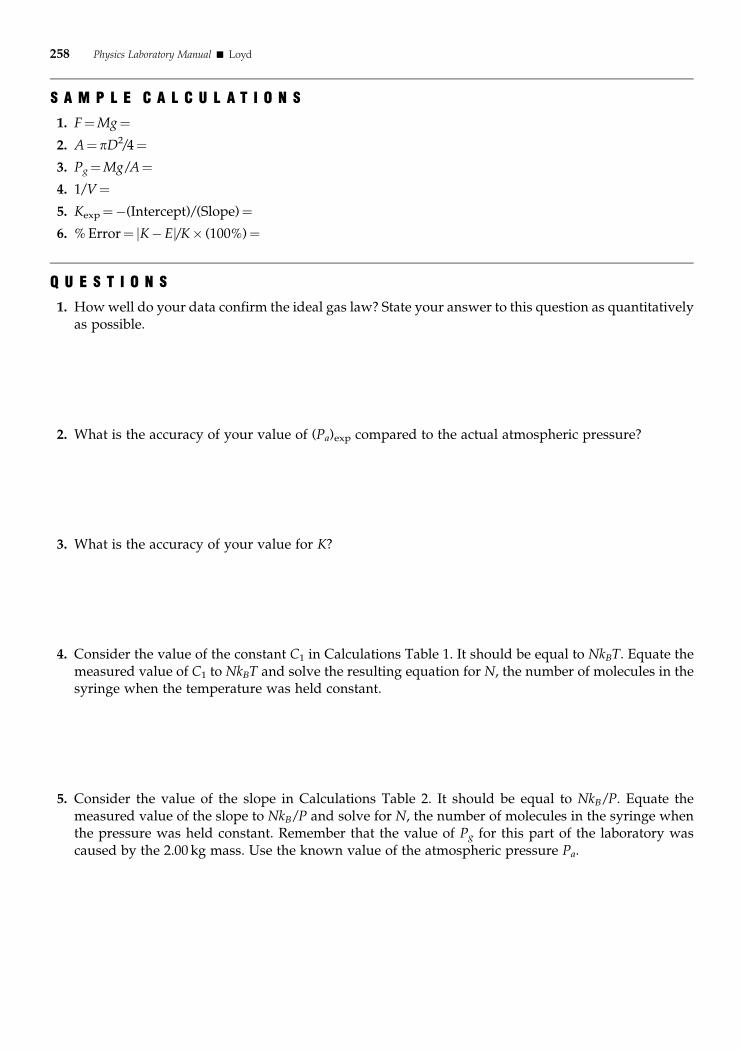
S A M P L E C A L C U L A T I O N S1. F¼Mg¼2. A¼ pD2/4¼3. Pg¼Mg/A¼4. 1/V¼5. Kexp¼�(Intercept)/(Slope)¼6. %Error¼ jK�Ej/K� (100%)¼
Q U E S T I O N S1. Howwell do your data confirm the ideal gas law? State your answer to this question as quantitatively
as possible.
2. What is the accuracy of your value of (Pa)exp compared to the actual atmospheric pressure?
3. What is the accuracy of your value for K?
4. Consider the value of the constant C1 in Calculations Table 1. It should be equal to NkBT. Equate themeasured value of C1 to NkBT and solve the resulting equation for N, the number of molecules in thesyringe when the temperature was held constant.
5. Consider the value of the slope in Calculations Table 2. It should be equal to NkB/P. Equate themeasured value of the slope to NkB/P and solve for N, the number of molecules in the syringe whenthe pressure was held constant. Remember that the value of Pg for this part of the laboratory wascaused by the 2.00 kg mass. Use the known value of the atmospheric pressure Pa.
258 Physics Laboratory Manual n Loyd

Equipotentials and ElectricFields
O B J E C T I V E So Investigate the location and shape of equipotential surfaces near oppositely charged electrodes
and construct electric field lines perpendicular to the equipotentials.
o Compare experimentally determined electric field lines with known patterns for line charge, twoline charges of opposite sign, and parallel plates.
o Determine the dependence of the magnitude of E on distance from a line of charge.
E Q U I P M E N T L I S T. Corkboard and push pins to attach power supply and voltmeter to electrodes
. Carbon-impregnated resistance paper with a grid
. Conducting paint or conducting pen (either silver-based or carbon-based)
. Direct current power supply (20V, low current)
. High impedance voltmeter (preferably digital)
T H E O R YConsider two electrodes of arbitrary shape some distance apart carrying equal and opposite charges.A potential difference of 20V exists between the electrodes with the negative electrode at zero and thepositive electrode at þ20V. In the space surrounding these electrodes, there are points at the samepotential. There will be some points with potentialþ10V. There will be other points with potentialþ15V,and still other points with potentialþ5V. In three dimensions all points with the same potential will forma surface. In fact, there will exist an infinite number of surfaces because the 20V total potential differencecan be divided into an infinite number of steps. Each surface with the same value of potential (voltage) iscalled an equipotential surface. In this laboratory we will determine the equipotentials associated with afew often used electrode configurations.
In addition to equipotential surfaces in the region around charged electrodes there is also presentan electric field. By definition the electric field is a vector field that can be represented by lines drawnfrom the positively charged electrode to the negatively charged electrode. The direction of the electricfield line at any point in space is the direction of the force that would be exerted on a positive test chargeplaced at that point in space. To ensure that the test charge does not disturb the other charges, the test
Physics Laboratory Manual n Loyd L A B O R A T O R Y 26
COPYRIG
HTª
2008ThomsonBrooks/Cole
259
ª 2008 Thomson Brooks/Cole, a part of TheThomson Corporation.Thomson, the Star logo, and Brooks/Cole are trademarks used herein under license. ALL RIGHTSRESERVED.No part of this workcovered by the copyright hereonmay be reproduced or used in any form or by any meansçgraphic, electronic, ormechanical, including photocopying, recording, taping,web distribution, informationstorage and retrieval systems,or in any othermannerçwithout the written permission of the publisher.
charge must be small. In fact, in the exact definition, the limit must be taken as the test charge approacheszero. The magnitude of the electric field is the force per unit charge on the positive test charge as themagnitude of the test charge approaches zero. The units of electric field are N/C. The number of field linesper unit area at a given point is a measure of the magnitude of the electric field. Thus a region where thereare a large number of lines per unit area is a region of large electric field.
The geometrical relationship that electric field lines have with equipotential surfaces is that electricfield lines are everywhere perpendicular to the equipotential surfaces. Electrodes themselves are equi-potential surfaces, so electric field lines must intersect electrodes perpendicularly. This is a helpful guideto determine the shape of electric fields around an electrode arrangement.
For two points separated by a very small distance Dxwith potential difference DV between the points,the electric field E is
E ¼ �DVDx
ðEq: 1Þ
Equation 1 shows that another proper unit for the electric field is V/m. Because the electrodes on thecarbon paper are limited to two dimensions, they represent a slice taken through a real three-dimensionalelectrode configuration. Therefore, the equipotentials mapped in this laboratory will be lines rather thansurfaces. Any two-dimensional electrode arrangement can be produced by drawing the desired elec-trode shape on the carbon paper with a conducting pen and then attaching a direct current powersupply between the electrodes. We will choose the electrode to which the negative terminal of thepower supply is attached to be the zero of potential, and will take all measurements relative to thatelectrode. We will use a voltmeter to find the points on the paper in the region of the electrodes that areat some given value of potential. When enough points are located to establish the shape of the equipo-tential, the equipotential line can be constructed by joining the points with a smooth curve. The studentmust decide the number of data points needed to establish the shape.
E X P E R I M E N T A L P R O C E D U R E1. Use a conductive ink pen to draw the three electrode configurations shown in Figure 26-2. Note the
following cautions: (a) Place the conductive paper on a hard surface, not on the corkboard to drawthe electrodes. (b) Make sure that the ink flows smoothly and evenly when drawing electrodes, andthat a solid line is obtained.
260 Physics Laboratory Manual n Loyd
Image not available due to copyright restrictions
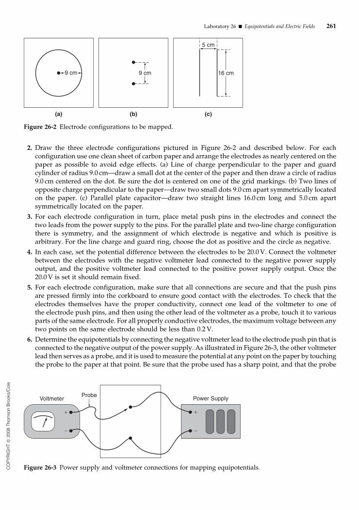
2. Draw the three electrode configurations pictured in Figure 26-2 and described below. For eachconfiguration use one clean sheet of carbon paper and arrange the electrodes as nearly centered on thepaper as possible to avoid edge effects. (a) Line of charge perpendicular to the paper and guardcylinder of radius 9.0 cm—draw a small dot at the center of the paper and then draw a circle of radius9.0 cm centered on the dot. Be sure the dot is centered on one of the grid markings. (b) Two lines ofopposite charge perpendicular to the paper—draw two small dots 9.0 cm apart symmetrically locatedon the paper. (c) Parallel plate capacitor—draw two straight lines 16.0 cm long and 5.0 cm apartsymmetrically located on the paper.
3. For each electrode configuration in turn, place metal push pins in the electrodes and connect thetwo leads from the power supply to the pins. For the parallel plate and two-line charge configurationthere is symmetry, and the assignment of which electrode is negative and which is positive isarbitrary. For the line charge and guard ring, choose the dot as positive and the circle as negative.
4. In each case, set the potential difference between the electrodes to be 20.0V. Connect the voltmeterbetween the electrodes with the negative voltmeter lead connected to the negative power supplyoutput, and the positive voltmeter lead connected to the positive power supply output. Once the20.0V is set it should remain fixed.
5. For each electrode configuration, make sure that all connections are secure and that the push pinsare pressed firmly into the corkboard to ensure good contact with the electrodes. To check that theelectrodes themselves have the proper conductivity, connect one lead of the voltmeter to one ofthe electrode push pins, and then using the other lead of the voltmeter as a probe, touch it to variousparts of the same electrode. For all properly conductive electrodes, the maximum voltage between anytwo points on the same electrode should be less than 0.2V.
6. Determine the equipotentials by connecting the negative voltmeter lead to the electrode push pin that isconnected to the negative output of the power supply. As illustrated in Figure 26-3, the other voltmeterlead then serves as a probe, and it is used tomeasure the potential at any point on the paper by touchingthe probe to the paper at that point. Be sure that the probe used has a sharp point, and that the probe
COPYRIG
HTª
2008ThomsonBrooks/Cole
9 cm
(a) (b) (c)
5 cm
9 cm 16 cm
Figure 26-2 Electrode configurations to be mapped.
Power SupplyVoltmeterProbe
�
�
�
�
Figure 26-3 Power supply and voltmeter connections for mapping equipotentials.
Laboratory 26 n Equipotentials and Electric Fields 261
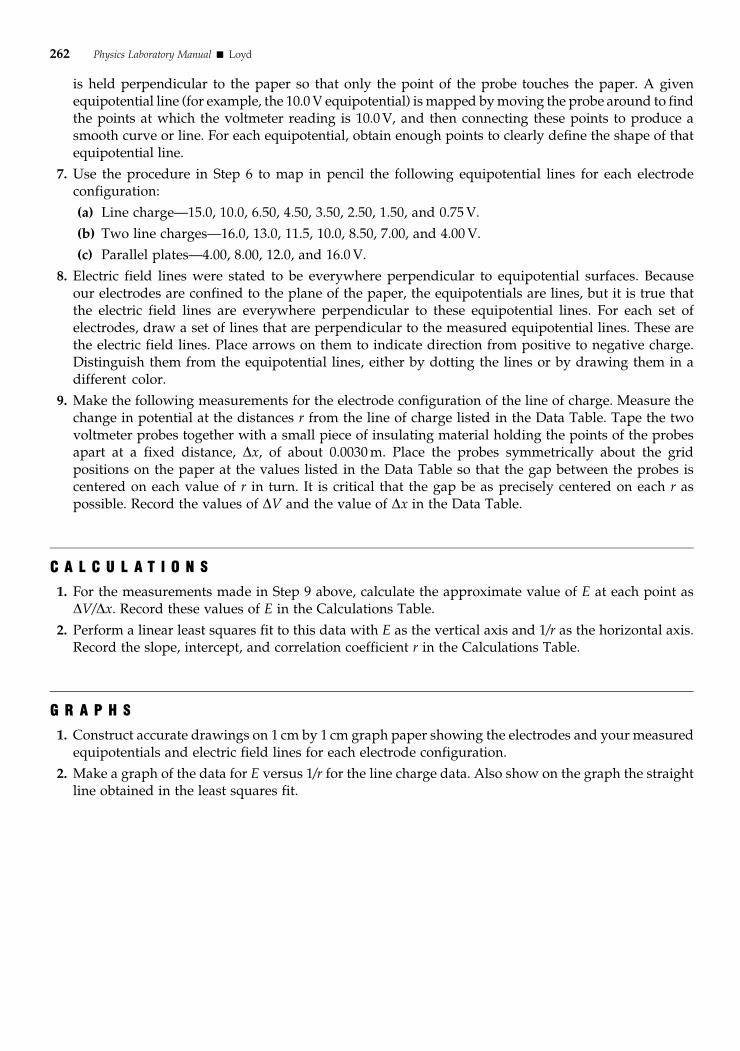
is held perpendicular to the paper so that only the point of the probe touches the paper. A givenequipotential line (for example, the 10.0V equipotential) ismapped bymoving the probe around to findthe points at which the voltmeter reading is 10.0V, and then connecting these points to produce asmooth curve or line. For each equipotential, obtain enough points to clearly define the shape of thatequipotential line.
7. Use the procedure in Step 6 to map in pencil the following equipotential lines for each electrodeconfiguration:
(a) Line charge—15.0, 10.0, 6.50, 4.50, 3.50, 2.50, 1.50, and 0.75V.
(b) Two line charges—16.0, 13.0, 11.5, 10.0, 8.50, 7.00, and 4.00V.
(c) Parallel plates—4.00, 8.00, 12.0, and 16.0V.
8. Electric field lines were stated to be everywhere perpendicular to equipotential surfaces. Becauseour electrodes are confined to the plane of the paper, the equipotentials are lines, but it is true thatthe electric field lines are everywhere perpendicular to these equipotential lines. For each set ofelectrodes, draw a set of lines that are perpendicular to the measured equipotential lines. These arethe electric field lines. Place arrows on them to indicate direction from positive to negative charge.Distinguish them from the equipotential lines, either by dotting the lines or by drawing them in adifferent color.
9. Make the following measurements for the electrode configuration of the line of charge. Measure thechange in potential at the distances r from the line of charge listed in the Data Table. Tape the twovoltmeter probes together with a small piece of insulating material holding the points of the probesapart at a fixed distance, Dx, of about 0.0030m. Place the probes symmetrically about the gridpositions on the paper at the values listed in the Data Table so that the gap between the probes iscentered on each value of r in turn. It is critical that the gap be as precisely centered on each r aspossible. Record the values of DV and the value of Dx in the Data Table.
C A L C U L A T I O N S1. For the measurements made in Step 9 above, calculate the approximate value of E at each point as
DV/Dx. Record these values of E in the Calculations Table.
2. Perform a linear least squares fit to this data with E as the vertical axis and 1/r as the horizontal axis.Record the slope, intercept, and correlation coefficient r in the Calculations Table.
G R A P H S1. Construct accurate drawings on 1 cm by 1 cm graph paper showing the electrodes and your measured
equipotentials and electric field lines for each electrode configuration.
2. Make a graph of the data for E versus 1/r for the line charge data. Also show on the graph the straightline obtained in the least squares fit.
262 Physics Laboratory Manual n Loyd

Name . . . . . . . . . . . . . . . . . . . . . . . . . . . . . . . . . . . . . . . . . . . . . . . . . . . . . . . . . . . . . . . . . . . . . . . . . Section . . . . . . . . . . . . . . . . Date . . . . . . . . . . . . . . . .
26 L A B O R A T O R Y 2 6 Equipotentials and Electric Fields
P R E - L A B O R A T O R Y A S S I G N M E N T1. Electric field lines are drawn (a) from positive charges to negative charges (b) from negative charges to
positive charges (c) from the largest charge to the smallest charge (d) from the smallest charge to thelargest charge.
2. The points where the potential is the same (in three-dimensional space) have the same voltage.(a) True (b) False
3. The points where the potential is the same (in three-dimensional space) lie on a surface. (a) True(b) False
4. The relationship between the direction of the electric field lines and the equipotential surfaces is(a) field lines are everywhere parallel to surfaces (b) field lines always intersect each other (c) fieldlines are everywhere perpendicular to surfaces (d) field lines always make angles between 08 and 908with surfaces.
5. Why are the measured equipotentials lines instead of surfaces for this laboratory?
6. If two electrodes have a source of potential difference of 100V connected to them, how manyequipotential surfaces exist in the space between them?
7. Why is it important to center the electrodes on the resistance paper for this laboratory?
COPYRIG
HTª
2008ThomsonBrooks/Cole
263

8. In the performance of this laboratory, what is the recommended maximum allowed potentialdifference from one end of an electrode to the other end?
9. On what basis are you to decide how many points to measure for each equipotential for a givenelectrode configuration?
264 Physics Laboratory Manual n Loyd

Name . . . . . . . . . . . . . . . . . . . . . . . . . . . . . . . . . . . . . . . . . . . . . . . . . . . . . . . . . . . . . . . . . . . . . . . . . Section . . . . . . . . . . . . . . . . Date . . . . . . . . . . . . . . . .
Lab Partners . . . . . . . . . . . . . . . . . . . . . . . . . . . . . . . . . . . . . . . . . . . . . . . . . . . . . . . . . . . . . . . . . . . . . . . . . . . . . . . . . . . . . . . . . . . . . . . . . . . . . . . . . . . . . . . . . . . .
26 L A B O R A T O R Y 2 6 Equipotentials and Electric Fields
L A B O R A T O R Y R E P O R T
S A M P L E C A L C U L A T I O N S1. E¼DV/Dx¼2. 1/r¼
COPYRIG
HTª
2008ThomsonBrooks/Cole
Data Table
r (m) DV (V)
0.0150
0.0200
0.0300
0.0400
0.0500
0.0600
0.0700
0.0800
Dx¼ m
Calculations Table
E ¼ �DVDx
ðV=mÞ 1/r (m�1)
Slope¼ Intercept¼ r¼
265
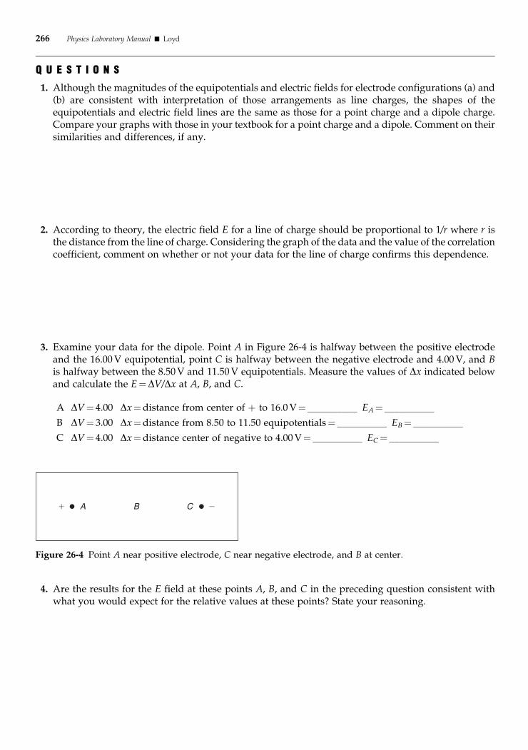
Q U E S T I O N S1. Although the magnitudes of the equipotentials and electric fields for electrode configurations (a) and
(b) are consistent with interpretation of those arrangements as line charges, the shapes of theequipotentials and electric field lines are the same as those for a point charge and a dipole charge.Compare your graphs with those in your textbook for a point charge and a dipole. Comment on theirsimilarities and differences, if any.
2. According to theory, the electric field E for a line of charge should be proportional to 1/r where r isthe distance from the line of charge. Considering the graph of the data and the value of the correlationcoefficient, comment on whether or not your data for the line of charge confirms this dependence.
3. Examine your data for the dipole. Point A in Figure 26-4 is halfway between the positive electrodeand the 16.00V equipotential, point C is halfway between the negative electrode and 4.00V, and Bis halfway between the 8.50V and 11.50V equipotentials. Measure the values of Dx indicated belowand calculate the E¼DV/Dx at A, B, and C.
A DV¼ 4.00 Dx¼distance from center of þ to 16.0V¼ __________ EA¼ __________
B DV¼ 3.00 Dx¼distance from 8.50 to 11.50 equipotentials¼ __________ EB¼ __________
C DV¼ 4.00 Dx¼distance center of negative to 4.00V¼ __________ EC¼ __________
4. Are the results for the E field at these points A, B, and C in the preceding question consistent withwhat you would expect for the relative values at these points? State your reasoning.
A B C� �
Figure 26-4 Point A near positive electrode, C near negative electrode, and B at center.
266 Physics Laboratory Manual n Loyd
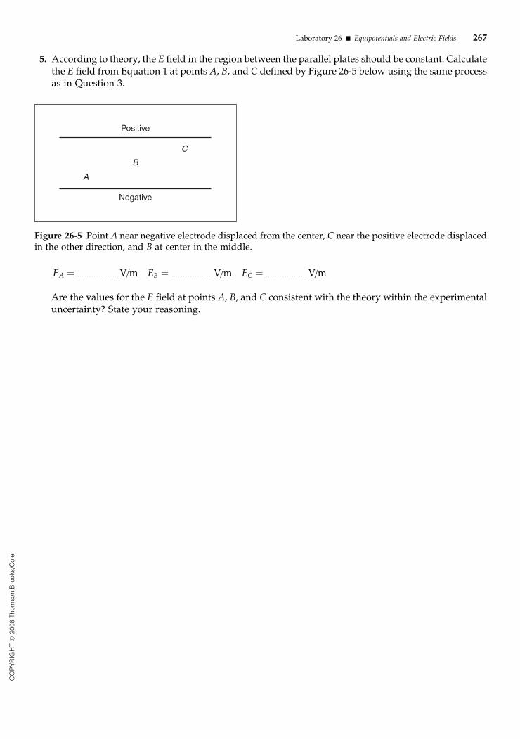
5. According to theory, the E field in the region between the parallel plates should be constant. Calculatethe E field from Equation 1 at points A, B, and C defined by Figure 26-5 below using the same processas in Question 3.
EA ¼ V=m EB ¼ V=m EC ¼ V=m
Are the values for the E field at points A, B, and C consistent with the theory within the experimentaluncertainty? State your reasoning.
COPYRIG
HTª
2008ThomsonBrooks/Cole
A
B
Positive
Negative
C
Figure 26-5 Point A near negative electrode displaced from the center, C near the positive electrode displacedin the other direction, and B at center in the middle.
Laboratory 26 n Equipotentials and Electric Fields 267

This page intentionally left blank

Capacitance Measurementwith a BallisticGalvanometer
O B J E C T I V E So Determine the deflection of a ballistic galvanometer for several capacitors of known capacitance
charged to a known voltage.
o Demonstrate that for a fixed voltage the galvanometer deflection is proportional to the capaci-tance of each capacitor.
o Determine the capacitance of unknown capacitors from galvanometer deflection.
o Experimentally determine the capacitance of series and parallel combinations of capacitors andcompare the results with theoretical predictions.
E Q U I P M E N T L I S T. Ballistic galvanometer, support stand, telescope, and scale
. Direct current power supply (0–20 V), direct current voltmeter (0–20 V)
. Five or six known capacitors in range 0.5–3.0 mF (can be in form of decade box)
. Three capacitors to serve as unknowns (1–2 mF), switch (single pole, double throw)
T H E O R YFigure 27-1 shows a capacitor of capacitance Cwith a voltageV across the plates. The figure illustrates thefact that a capacitor, with a charge of Q, has a charge of þQ on one plate and –Q on the other plate.Therefore, the net charge on a capacitor is always zero. The relationship between capacitance C, voltageV,and charge Q is
C ¼ Q
VðEq: 1Þ
The units of capacitance (Coulomb/Volt) have been given the name farad with symbol F.
Physics Laboratory Manual n Loyd L A B O R A T O R Y 27
COPYRIG
HTª
2008ThomsonBrooks/Cole
269
ª 2008 Thomson Brooks/Cole, a part of TheThomson Corporation.Thomson, the Star logo, and Brooks/Cole are trademarks used herein under license. ALL RIGHTSRESERVED.No part of this workcovered by the copyright hereonmay be reproduced or used in any form or by any meansçgraphic, electronic, ormechanical, including photocopying, recording, taping,web distribution, informationstorage and retrieval systems,or in any othermannerçwithout the written permission of the publisher.
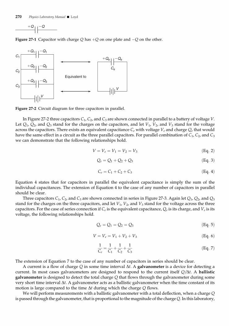
In Figure 27-2 three capacitors C1, C2, and C3 are shown connected in parallel to a battery of voltage V.Let Q1, Q2, and Q3 stand for the charges on the capacitors, and let V1, V2, and V3 stand for the voltageacross the capacitors. There exists an equivalent capacitance Ce with voltage Ve and charge Qe that wouldhave the same effect in a circuit as the three parallel capacitors. For parallel combination of C1, C2, and C3
we can demonstrate that the following relationships hold.
V ¼ Ve ¼ V1 ¼ V2 ¼ V3 ðEq: 2Þ
Qe ¼ Q1 þQ2 þQ3 ðEq: 3Þ
Ce ¼ C1 þ C2 þ C3 ðEq: 4Þ
Equation 4 states that for capacitors in parallel the equivalent capacitance is simply the sum of theindividual capacitances. The extension of Equation 4 to the case of any number of capacitors in parallelshould be clear.
Three capacitors C1, C2, and C3 are shown connected in series in Figure 27-3. Again let Q1, Q2, and Q3
stand for the charges on the three capacitors, and let V1, V2, and V3 stand for the voltage across the threecapacitors. For the case of series connection if Ce is the equivalent capacitance,Qe is its charge, and Ve is itsvoltage, the following relationships hold.
Qe ¼ Q1 ¼ Q2 ¼ Q3 ðEq: 5Þ
V ¼ Ve ¼ V1 þ V2 þ V3 ðEq: 6Þ1
Ce¼ 1
C1þ 1
C2þ 1
C3ðEq: 7Þ
The extension of Equation 7 to the case of any number of capacitors in series should be clear.A current is a flow of charge Q in some time interval Dt. A galvanometer is a device for detecting a
current. In most cases galvanometers are designed to respond to the current itself Q/Dt. A ballisticgalvanometer is designed to detect the total charge Q that flows through the galvanometer during somevery short time interval Dt. A galvanometer acts as a ballistic galvanometer when the time constant of itsmotion is large compared to the time Dt during which the charge Q flows.
We will performmeasurements with a ballistic galvanometer with a total deflection, when a chargeQis passed through the galvanometer, that is proportional to themagnitude of the chargeQ. In this laboratory,
�Q1C1
�Q1
�Q2 �Q2
�Q3�Q3
V
C2
C3
�Qe �Qe
Ce
V
Equivalent to
Figure 27-2 Circuit diagram for three capacitors in parallel.
�Q �Q
Figure 27-1 Capacitor with charge Q has þQ on one plate and �Q on the other.
270 Physics Laboratory Manual n Loyd
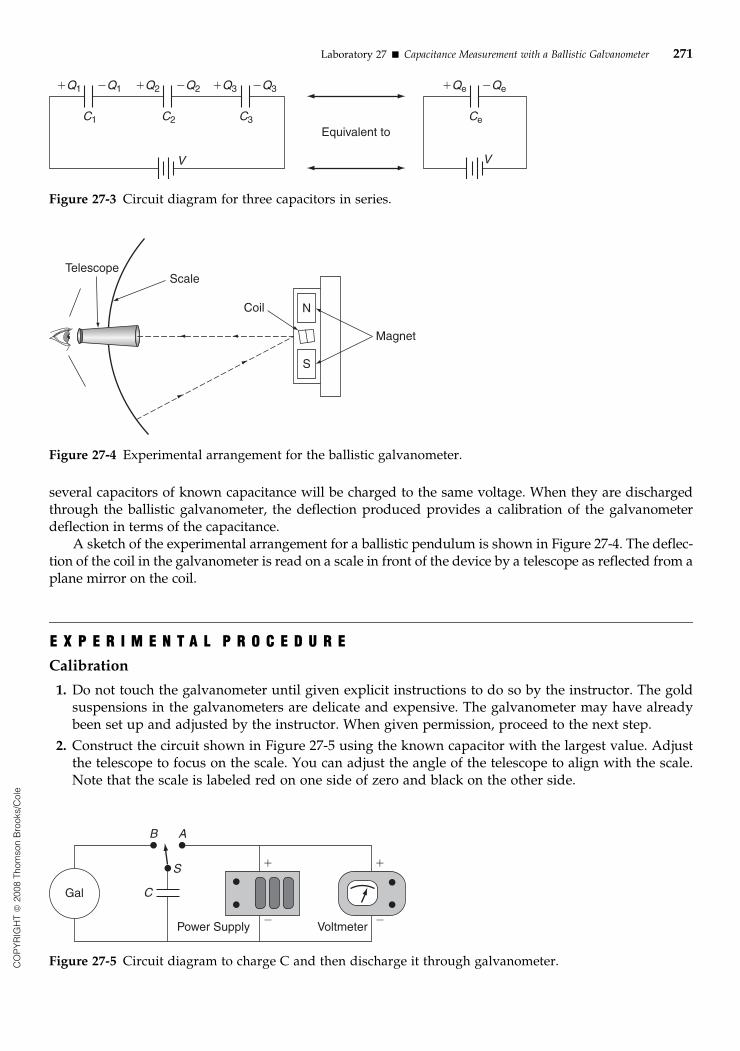
several capacitors of known capacitance will be charged to the same voltage. When they are dischargedthrough the ballistic galvanometer, the deflection produced provides a calibration of the galvanometerdeflection in terms of the capacitance.
A sketch of the experimental arrangement for a ballistic pendulum is shown in Figure 27-4. The deflec-tion of the coil in the galvanometer is read on a scale in front of the device by a telescope as reflected from aplane mirror on the coil.
E X P E R I M E N T A L P R O C E D U R ECalibration
1. Do not touch the galvanometer until given explicit instructions to do so by the instructor. The goldsuspensions in the galvanometers are delicate and expensive. The galvanometer may have alreadybeen set up and adjusted by the instructor. When given permission, proceed to the next step.
2. Construct the circuit shown in Figure 27-5 using the known capacitor with the largest value. Adjustthe telescope to focus on the scale. You can adjust the angle of the telescope to align with the scale.Note that the scale is labeled red on one side of zero and black on the other side.
COPYRIG
HTª
2008ThomsonBrooks/Cole
�Q3
C3
�Q3�Q2
C2
�Q2�Q1
C1
�Q1
V
�Qe �Qe
Ce
V
Equivalent to
Figure 27-3 Circuit diagram for three capacitors in series.
TelescopeScale
Coil N
S
Magnet
Figure 27-4 Experimental arrangement for the ballistic galvanometer.
VoltmeterPower Supply
Gal C
S
AB
�
�
�
�
Figure 27-5 Circuit diagram to charge C and then discharge it through galvanometer.
Laboratory 27 n Capacitance Measurement with a Ballistic Galvanometer 271

3. Using the largest known capacitor, charge the capacitor to some known voltage by throwing switch Sto position A. Discharge the capacitor through the galvanometer by throwing the switch to position B.Adjust the voltage applied to the capacitor until it produces approximately 90% deflection for thiscapacitor. Record that value of voltage as V in Data and Calculations Tables 1 and 2. Make all mea-surements with this voltage.
4. Measure the deflection for each of the known capacitors when they have been charged with voltage Vand then discharged through the galvanometer. Perform three trials for each capacitor. Record thevalues of the deflection D and the known value of each capacitor in Data and Calculations Table 1.
Unknown Capacitance
1. Label the three unknown capacitors C1, C2, and C3. For each of the unknown capacitors, determine thedeflectionof thegalvanometerwhen theyhavebeen charged tovoltageVand thendischarged through thegalvanometer. Perform three trials for each capacitor. Record the value of the deflection D for each trial.
2. Connect capacitorsC1 andC2 in parallel and place them in the circuit in the position ofC in Figure 27-5.Determine the deflectionwhen the combination is chargedwith voltageV and then discharged throughthe galvanometer. Record the deflections in Data and Calculations Table 2. Repeat with capacitorsC2 and C3 in parallel.
3. Connect capacitors C1 and C2 in series and place them in the circuit in the position of capacitor Cin Figure 27-5. Determine the deflection when the combination is charged with voltage V and thendischarged through the galvanometer. Record the deflections in Data and Calculations Table 2. Repeatwith capacitors C2 and C3 in series.
C A L C U L A T I O N SCalibration
1. Calculate the mean D and standard error aD for the three trials for each capacitor and record them inData and Calculations Table 1.
2. Perform a linear least squares fit to the data with the C as the vertical axis andD as the horizontal axis.Record the slope K, the intercept I, and the correlation coefficient r in Data and Calculations Table 1.
Unknown Capacitance
1. Calculate the mean D and standard error aD for each of the three trials. Record them in Data andCalculations Table 2.
2. For the individual capacitors, the series combinations, and the parallel combinations, calculate theexperimental values for the capacitance from Cexp ¼ KDþ I where K is the slope and I is the interceptof the least squares fit. The slope K has units of mF/deflection, and the intercept has units of mF. Recordthese values of the experimental capacitance in Data and Calculations Table 2.
3. Calculate a theoretical value for the series and parallel combinations of the capacitors usingEquations 4 and 7. In the calculations, use the measured values for the individual capacitors. Recordthese theoretical values for the series and parallel combinations in Data and Calculations Table 2 in theappropriate places.
4. Calculate the percentage difference between the experimental and theoretical values for the series andparallel combinations and record them in Data and Calculations Table 2.
G R A P H S1. Make a graph with the capacitance C as the vertical axis and the deflection D as the horizontal axis.
Also show on the graph the straight line obtained by the linear least squares fit to the data.
272 Physics Laboratory Manual n Loyd

Name . . . . . . . . . . . . . . . . . . . . . . . . . . . . . . . . . . . . . . . . . . . . . . . . . . . . . . . . . . . . . . . . . . . . . . . . . Section . . . . . . . . . . . . . . . . Date . . . . . . . . . . . . . . . .
27 L A B O R A T O R Y 2 7 Capacitance Measurement with a BallisticGalvanometer
P R E - L A B O R A T O R Y A S S I G N M E N T1. What is the definition of capacitance?
2. What are the units of capacitance?
3. A capacitor is said to have a charge of 10 mC.What is the charge on the positively charged plate? Whatis the charge on the negatively charged plate?
4. A 1.50 mF capacitor has a voltage across the plates of 6.00 V. What is the charge on the capacitor? Showyour work.
COPYRIG
HTª
2008ThomsonBrooks/Cole
273

5. Which of the following are true for three capacitors C1, C2, and C3 in parallel with a battery of voltageV? More than one answer may be true.
(a) V¼V1¼V2¼V3 (b) Qe¼Q1¼Q2¼Q3 (c) Qe¼Q1 þ Q2 þ Q3 (d) V¼V1 þ V2 þ V3
6. Which of the following are true for three capacitors C1, C2, and C3 in series with a battery of voltage V?More than one answer may be true.
(a) V¼V1¼V2¼V3 (b) Qe¼Q1¼Q2¼Q3 (c) Qe¼Q1 þ Q2 þ Q3 (d) V¼V1 þ V2 þ V3
7. Three capacitors of capacitance 5.00 mF, 8.00 mF, and 11.00 mF are connected in parallel. What is theequivalent capacitance of the combination? Show your work.
8. Three capacitors of capacitance 5.00 mF, 8.00 mF, and 11.00 mF are connected in series. What is theequivalent capacitance of the combination? Show your work.
274 Physics Laboratory Manual n Loyd

Name . . . . . . . . . . . . . . . . . . . . . . . . . . . . . . . . . . . . . . . . . . . . . . . . . . . . . . . . . . . . . . . . . . . . . . . . . Section . . . . . . . . . . . . . . . . Date . . . . . . . . . . . . . . . .
Lab Partners . . . . . . . . . . . . . . . . . . . . . . . . . . . . . . . . . . . . . . . . . . . . . . . . . . . . . . . . . . . . . . . . . . . . . . . . . . . . . . . . . . . . . . . . . . . . . . . . . . . . . . . . . . . . . . . . . . . .
27 L A B O R A T O R Y 2 7 Capacitance Measurement with a BallisticGalvanometer
L A B O R A T O R Y R E P O R T
Data and Calculations Table 1
C (mF) D1 D2 D3 D aD
V¼ volts K¼ mF/defl I¼ mF r¼
Data and Calculations Table 2
Capacitor D1 D2 D3 D aD Cexp Ctheo % Diff
C1
C2
C3
C1 & C2 Parallel
C2 & C3 Parallel
C1 & C2 Series
C2 & C3 Series
V¼ volts
COPYRIG
HTª
2008ThomsonBrooks/Cole
275

S A M P L E C A L C U L A T I O N S1. Cexp ¼ KDþ I ¼2. (Parallel) Ctheo¼C1þC2¼3. (Series) (1/Ctheo)¼ (1/C1)þ (1/C2)¼4. % Diff¼5. % Error (if actual values for unknown are given)¼
Q U E S T I O N S1. What is the precision of your measurements of the unknown capacitors? State clearly the basis for
your answer.
2. If possible, obtain values for the unknown capacitors. Determine the accuracy of your measurementsof the capacitance if these values are available.
3. Based on the precision and accuracy of your results, is there any evidence for a systematic error in themeasurements? State clearly the basis for your answer.
4. How well do your data confirm the theoretical equations for the parallel combination of capacitors?Answer the question as quantitatively as possible.
276 Physics Laboratory Manual n Loyd

5. How well do your data confirm the theoretical equation for the series combination of capacitors?Answer the question as quantitatively as possible.
6. Suppose that you were given an unknown capacitor with a value of about twice as large as the largestknown capacitor that you measured. What simple change in the procedure would allow you todetermine an approximate value for its capacitance using the value for K that you have alreadydetermined?
COPYRIG
HTª
2008ThomsonBrooks/Cole
Laboratory 27 n Capacitance Measurement with a Ballistic Galvanometer 277

This page intentionally left blank
Measurement of ElectricalResistance and Ohm’s Law
O B J E C T I V E So Define the concept of electrical resistance using measurements of the voltage across and current
in a wire coil.
o Investigate the dependence of the resistance on the length, cross-sectional area, and resistivity ofthe wire.
o Investigate the equivalent resistance of series and parallel resistors.
E Q U I P M E N T L I S T. Resistance coils (standard set available from Sargent-Welch or Central Scientific consisting of 10m and20m length of copper and German silver wire)
. Direct current ammeter (0–2A), direct current voltmeter (0–30V, preferably digital readout)
. Direct current power supply (0–20V at 1A)
T H E O R YIf a voltageV is applied across an element in an electrical circuit, the current I in the element is determinedby a quantity known as the resistance R. The relationship between these three quantities serves as adefinition of resistance.
R ¼ V
IðEq: 1Þ
The units of resistance are volt/ampere, which are given the name ohm. The symbol for ohm is O. Somecircuit elements obey a relationship known asOhm’s Law. For these elements the quantity R is a constantfor different values of V. If a circuit element obeys Ohm’s Law, when the voltage V is varied the current Iwill also vary, but the ratio V/I should remain constant. In this laboratory we will perform measurementson five coils ofwire to investigate if they obeyOhm’s Law.We alsowill determine the resistance of the coils.
The resistance of any object to electrical current is a function of the material from which it is con-structed, the length, the cross-sectional area, and the temperature of the object. At constant temperaturethe resistance R is given by
Physics Laboratory Manual n Loyd L A B O R A T O R Y 28
COPYRIG
HTª
2008ThomsonBrooks/Cole
279
ª 2008 Thomson Brooks/Cole, a part of TheThomson Corporation.Thomson, the Star logo, and Brooks/Cole are trademarks used herein under license. ALL RIGHTSRESERVED.No part of this workcovered by the copyright hereonmay be reproduced or used in any form or by any meansçgraphic, electronic, ormechanical, including photocopying, recording, taping,web distribution, informationstorage and retrieval systems,or in any othermannerçwithout the written permission of the publisher.
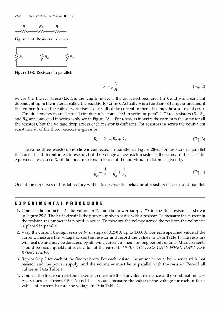
R ¼ rL
AðEq: 2Þ
where R is the resistance (O), L is the length (m), A is the cross-sectional area (m2), and r is a constantdependent upon the material called the resistivity (O�m). Actually r is a function of temperature, and ifthe temperature of the coils of wire rises as a result of the current in them, this may be a source of error.
Circuit elements in an electrical circuit can be connected in series or parallel. Three resistors (R1, R2,and R3) are connected in series as shown in Figure 28-1. For resistors in series the current is the same for allthe resistors, but the voltage drop across each resistor is different. For resistors in series the equivalentresistance Re of the three resistors is given by
Re ¼ R1 þ R2 þ R3 ðEq: 3Þ
The same three resistors are shown connected in parallel in Figure 28-2. For resistors in parallelthe current is different in each resistor, but the voltage across each resistor is the same. In this case theequivalent resistance Re of the three resistors in terms of the individual resistors is given by
1
Re¼ 1
R1þ 1
R2þ 1
R3ðEq: 4Þ
One of the objectives of this laboratory will be to observe the behavior of resistors in series and parallel.
E X P E R I M E N T A L P R O C E D U R E1. Connect the ammeter A, the voltmeterV, and the power supply PS to the first resistor as shown
in Figure 28-3. The basic circuit is the power supply in series with a resistor. To measure the current inthe resistor, the ammeter is placed in series. To measure the voltage across the resistor, the voltmeteris placed in parallel.
2. Vary the current through resistor R1 in steps of 0.250A up to 1.000A. For each specified value of thecurrent, measure the voltage across the resistor and record the values in Data Table 1. The resistorswill heat up andmay be damaged by allowing current in them for long periods of time.Measurementsshould be made quickly at each value of the current. APPLY VOLTAGE ONLY WHEN DATA AREBEING TAKEN.
3. Repeat Step 2 for each of the five resistors. For each resistor the ammeter must be in series with thatresistor and the power supply, and the voltmeter must be in parallel with the resistor. Record allvalues in Data Table 1.
4. Connect the first four resistors in series to measure the equivalent resistance of the combination. Usetwo values of current, 0.500A and 1.000A, and measure the value of the voltage for each of thesevalues of current. Record the voltage in Data Table 2.
R1 R2 R3
Figure 28-1 Resistors in series.
R1 R2 R3
Figure 28-2 Resistors in parallel.
280 Physics Laboratory Manual n Loyd
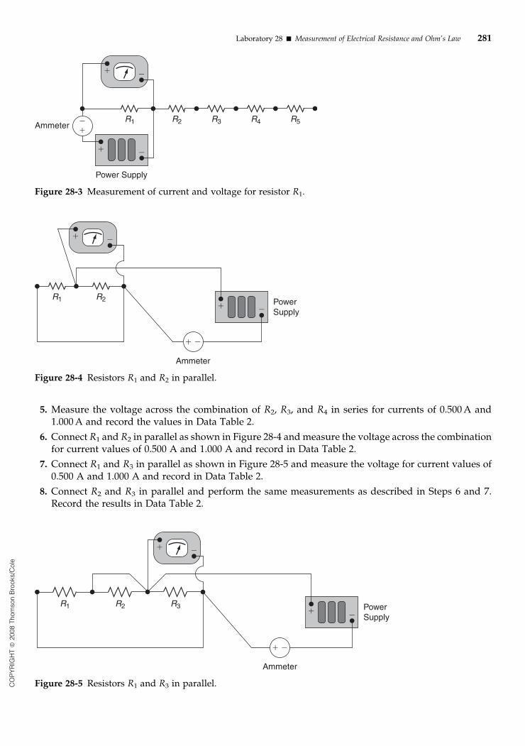
5. Measure the voltage across the combination of R2, R3, and R4 in series for currents of 0.500A and1.000A and record the values in Data Table 2.
6. Connect R1 and R2 in parallel as shown in Figure 28-4 andmeasure the voltage across the combinationfor current values of 0.500 A and 1.000 A and record in Data Table 2.
7. Connect R1 and R3 in parallel as shown in Figure 28-5 and measure the voltage for current values of0.500 A and 1.000 A and record in Data Table 2.
8. Connect R2 and R3 in parallel and perform the same measurements as described in Steps 6 and 7.Record the results in Data Table 2.
COPYRIG
HTª
2008ThomsonBrooks/Cole
R3R2
Power Supply
AmmeterR1 R4 R5
� �
� �
��
Figure 28-3 Measurement of current and voltage for resistor R1.
R2R1 PowerSupply
Ammeter
� �
� �
� �
Figure 28-4 Resistors R1 and R2 in parallel.
� �
� �
R3R2R1 PowerSupply
Ammeter
� �
Figure 28-5 Resistors R1 and R3 in parallel.
Laboratory 28 n Measurement of Electrical Resistance and Ohm’s Law 281
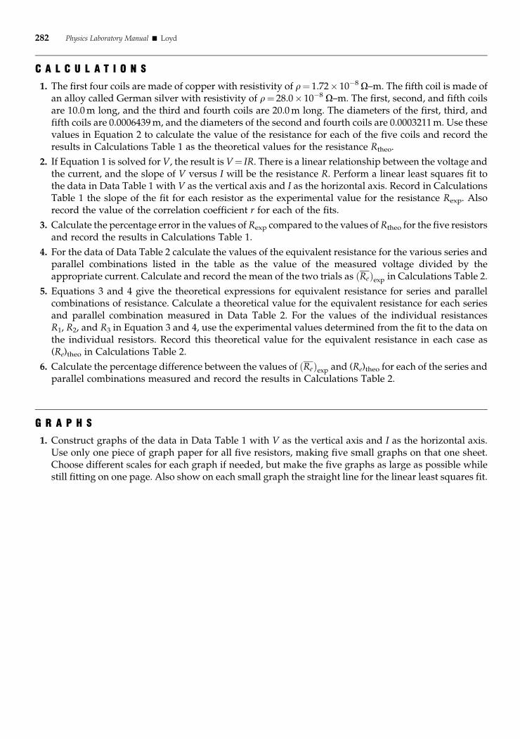
C A L C U L A T I O N S1. The first four coils are made of copper with resistivity of r¼ 1.72� 10�8 O–m. The fifth coil is made of
an alloy called German silver with resistivity of r¼ 28.0� 10�8 O–m. The first, second, and fifth coilsare 10.0m long, and the third and fourth coils are 20.0m long. The diameters of the first, third, andfifth coils are 0.0006439m, and the diameters of the second and fourth coils are 0.0003211m. Use thesevalues in Equation 2 to calculate the value of the resistance for each of the five coils and record theresults in Calculations Table 1 as the theoretical values for the resistance Rtheo.
2. If Equation 1 is solved for V, the result is V¼ IR. There is a linear relationship between the voltage andthe current, and the slope of V versus I will be the resistance R. Perform a linear least squares fit tothe data in Data Table 1 with V as the vertical axis and I as the horizontal axis. Record in CalculationsTable 1 the slope of the fit for each resistor as the experimental value for the resistance Rexp. Alsorecord the value of the correlation coefficient r for each of the fits.
3. Calculate the percentage error in the values of Rexp compared to the values ofRtheo for the five resistorsand record the results in Calculations Table 1.
4. For the data of Data Table 2 calculate the values of the equivalent resistance for the various series andparallel combinations listed in the table as the value of the measured voltage divided by theappropriate current. Calculate and record the mean of the two trials as ðReÞexp in Calculations Table 2.
5. Equations 3 and 4 give the theoretical expressions for equivalent resistance for series and parallelcombinations of resistance. Calculate a theoretical value for the equivalent resistance for each seriesand parallel combination measured in Data Table 2. For the values of the individual resistancesR1, R2, and R3 in Equation 3 and 4, use the experimental values determined from the fit to the data onthe individual resistors. Record this theoretical value for the equivalent resistance in each case as(Re)theo in Calculations Table 2.
6. Calculate the percentage difference between the values of ðReÞexp and (Re)theo for each of the series andparallel combinations measured and record the results in Calculations Table 2.
G R A P H S1. Construct graphs of the data in Data Table 1 with V as the vertical axis and I as the horizontal axis.
Use only one piece of graph paper for all five resistors, making five small graphs on that one sheet.Choose different scales for each graph if needed, but make the five graphs as large as possible whilestill fitting on one page. Also show on each small graph the straight line for the linear least squares fit.
282 Physics Laboratory Manual n Loyd
Name . . . . . . . . . . . . . . . . . . . . . . . . . . . . . . . . . . . . . . . . . . . . . . . . . . . . . . . . . . . . . . . . . . . . . . . . . Section . . . . . . . . . . . . . . . . Date . . . . . . . . . . . . . . . .
28 L A B O R A T O R Y 2 8 Measurement of Electrical Resistance and Ohm’s Law
P R E - L A B O R A T O R Y A S S I G N M E N T1. Three resistors R1, R2, and R3 are connected in series with R1 <R2 <R3. Choose all correct answers
below. The total resistance of the combination is (a) less than R1, (b) less than R3, (c) greater than R3,(d) greater than 3 R3, (e) equal to R1þR2þR3.
2. Two resistors R1 and R2 are connected in parallel with R1 <R2. Choose all correct answers below. Thetotal resistance of the combination is (a) less than R1, (b) less than R2, (c) greater than R2, (d) greaterthan 2 R2, (e) equal to (R1R2)/(R1þR2).
3. A wire of length L1 and diameter d1 has resistance R1. A second wire of the same material has lengthL2¼ 2 L1 and diameter d2¼ 2 d1. The resistance of wire two is R2. Choose the correct value for R2.(a) R2¼R1, (b) R2¼ 2R1, (c) R2¼½R1, (d) R2¼ 4R1.
4. If a circuit element carries a current of 3.71 A, and the voltage drop across the element is 8.69V, what isthe resistance of the circuit element? Show your work.
R¼ ____________________ O
5. A resistor is known to obey Ohm’s Law. When there is a current of 1.72 A in the resistor, it hasa voltage drop across its terminals of 7.35V. If a voltage of 12.0V is applied across the resistor, whatis the current in the resistor? Show your work.
I¼ ____________________ A
COPYRIG
HTª
2008ThomsonBrooks/Cole
283

6. The resistivity of copper is 1.72� 10�8 O–m. A copper wire is 15.0m long, and the wire diameter is0.0500 cm. What is the resistance of the wire? Show your work.
R¼ ____________________ O
7. Awire of cross-sectional area 5.00� 10�6 m2 has a resistance of 1.75 O. What is the resistance of a wireof the same material and length as the first wire, but with a cross-sectional area of 8.75� 10�6 m2?Show your work.
R¼ ____________________ O
8. Three resistors of resistance 20.0O, 30.0O, and 40.0O are connected in series. What is their equivalentresistance? Show your work.
R¼ ____________________ O
9. Three resistors of resistance 15.0O, 25.0O, and 35.0O are connected in parallel. What is theirequivalent resistance? Show your work.
R¼ ____________________ O
284 Physics Laboratory Manual n Loyd

Name . . . . . . . . . . . . . . . . . . . . . . . . . . . . . . . . . . . . . . . . . . . . . . . . . . . . . . . . . . . . . . . . . . . . . . . . . Section . . . . . . . . . . . . . . . . Date . . . . . . . . . . . . . . . .
Lab Partners . . . . . . . . . . . . . . . . . . . . . . . . . . . . . . . . . . . . . . . . . . . . . . . . . . . . . . . . . . . . . . . . . . . . . . . . . . . . . . . . . . . . . . . . . . . . . . . . . . . . . . . . . . . . . . . . . . . .
28 L A B O R A T O R Y 2 8 Measurement of Electrical Resistance and Ohm’s Law
L A B O R A T O R Y R E P O R T
COPYRIG
HTª
2008ThomsonBrooks/Cole
Data Table 1
I (A) VR1 (V) VR2 (V) VR3 (V) VR4 (V) VR5 (V)
0.250
0.500
0.750
1.000
Calculations Table 1
R1 R2 R3 R4 R5
Rtheo
Rexp
r
% Error Rexp
285
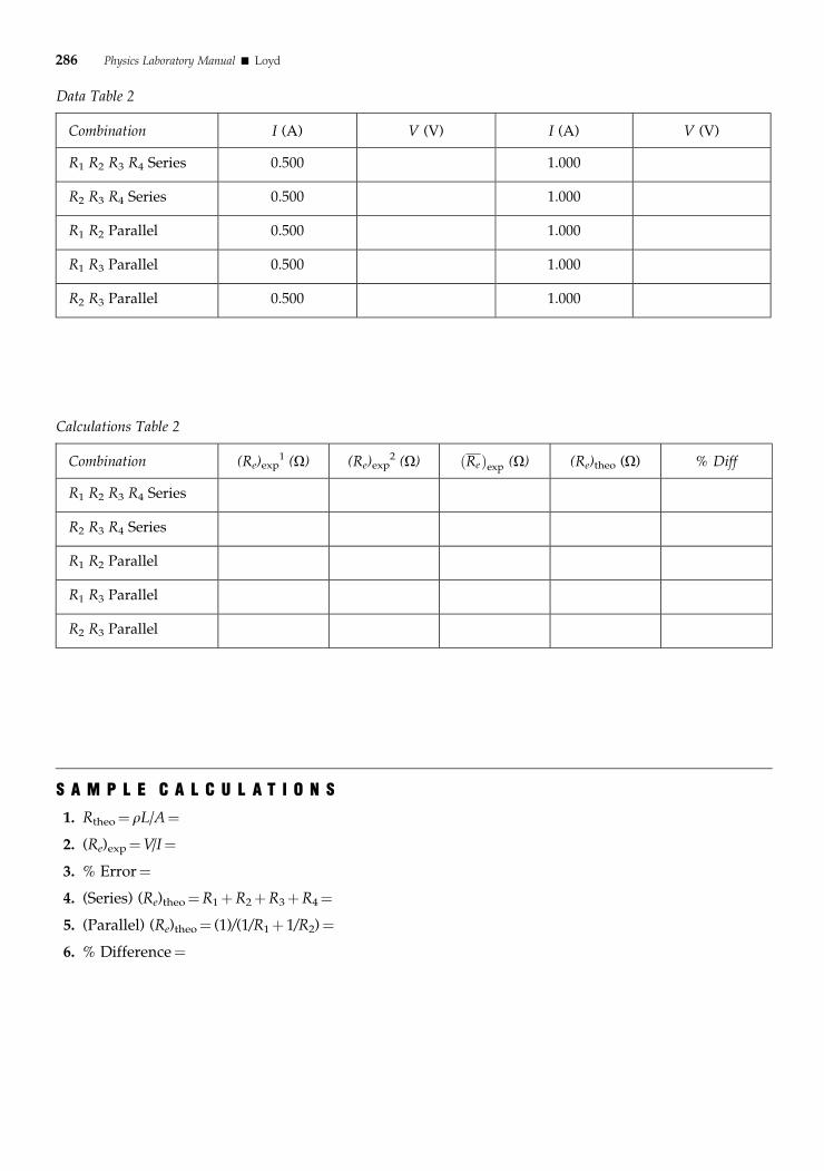
S A M P L E C A L C U L A T I O N S1. Rtheo¼rL/A¼2. (Re)exp¼V/I¼3. % Error¼4. (Series) (Re)theo¼R1þR2þR3þR4¼5. (Parallel) (Re)theo¼ (1)/(1/R1þ 1/R2)¼6. % Difference¼
Calculations Table 2
Combination (Re)exp1 (O) (Re)exp
2 (O) ðReÞexp (O) (Re)theo (O) % Diff
R1 R2 R3 R4 Series
R2 R3 R4 Series
R1 R2 Parallel
R1 R3 Parallel
R2 R3 Parallel
Data Table 2
Combination I (A) V (V) I (A) V (V)
R1 R2 R3 R4 Series 0.500 1.000
R2 R3 R4 Series 0.500 1.000
R1 R2 Parallel 0.500 1.000
R1 R3 Parallel 0.500 1.000
R2 R3 Parallel 0.500 1.000
286 Physics Laboratory Manual n Loyd
Q U E S T I O N S1. Do the individual resistors you havemeasured obey Ohm’s Law? In answering this question, consider
the least squares fits and the graphs you have made for each resistor. Remember that linear behaviorof V versus I is the proof of ohmic behavior.
2. Evaluate the agreement between the theoretical values for the individual resistances and the expe-rimental values.
3. Does your agreement between the experimental and theoretical values of the series combinations ofresistors support Equation 3 as the model for series combination of resistors? The agreement is notexpected to be perfect, but you are to determine if the agreement is reasonable within the expectedexperimental uncertainty.
4. Evaluate the agreement between the experimental and theoretical values of the parallel combinationsof resistors. Do the results support Equation 4 as the model for the parallel combination of resistorswithin the expected experimental uncertainty?
5. The first and second coils have the same length, and the third and fourth coils have the same length.They differ only in the cross-sectional area. According to theory, what should be the ratio of theresistance of the second coil to the first and the fourth coil to the third? Calculate these ratios for yourexperimental results and compare the agreement with the expected ratio.
COPYRIG
HTª
2008ThomsonBrooks/Cole
Laboratory 28 n Measurement of Electrical Resistance and Ohm’s Law 287

6. The first and third coils have the same cross-sectional area, and the second and fourth coils have thesame cross-sectional area. They differ only in length. According to theory, what should be the ratio ofthe resistance of the third coil to the first and the fourth coil to the second? Calculate these ratios foryour experimental results and compare the agreement with the expected ratio.
288 Physics Laboratory Manual n Loyd

Wheatstone Bridge
O B J E C T I V E So Investigate the principles of operation of a slide-wire formWheatstone bridge and determine the
resistance of several unknown resistors.
o Demonstrate the standard color code used to specify the value of commercially availableresistors.
E Q U I P M E N T L I S T. Slide-wire Wheatstone bridge, decade resistance box (1000O), galvanometer
. Switch with 10 kO resistor in parallel, direct current power supply
. Five color-coded resistors (in range 100 to 1000O) to serve as unknowns
. Assortment of circuit wires, multimeter with resistance scale
T H E O R YConsider a circuit that contains three resistors with values that are both known and adjustable, anunknown resistance, a power supply, and a galvanometer connected as shown in Figure 29-1. Current Ifrom the power supply divides at junction J. The current in R1 is I1, and the current in R3 is I2, whereI¼ I1þ I2. By experimentally varying the values of the resistances, a condition (known as the balancecondition) can be achieved where there is no current in the galvanometer G. This circuit is known as aWheatstone bridge.
When there is no current in the galvanometer, the current in R1 must go through R2, and both resistorshave current of I1. Similarly, when the balance condition holds, the current through R4 must be the sameas the current through R3, and thus it is equal to I2.
When there is no current in the galvanometer, there is no potential difference between points A and B,so these points are at the same potential. The change in potential from point J to point B (VJB) is equal tothe potential change from point J to point A (VJA), and
VJA ¼ I1R1 ¼ VJB ¼ I2R3 and thus I1R1 ¼ I2R3 ðEq: 1Þ
Similarly, the potential change across R2 (VAK) is the same as the potential change across R4 (VBK) so that
VAK ¼ I1R2 ¼ VBK ¼ I2R4 and thus I1R2 ¼ I2R4 ðEq: 2Þ
Physics Laboratory Manual n Loyd L A B O R A T O R Y 29
COPYRIG
HTª
2008ThomsonBrooks/Cole
289
ª 2008 Thomson Brooks/Cole, a part of TheThomson Corporation.Thomson, the Star logo, and Brooks/Cole are trademarks used herein under license. ALL RIGHTSRESERVED.No part of this workcovered by the copyright hereonmay be reproduced or used in any form or by any meansçgraphic, electronic, ormechanical, including photocopying, recording, taping,web distribution, informationstorage and retrieval systems,or in any othermannerçwithout the written permission of the publisher.

If Equation 1 is divided by Equation 2, the currents cancel, and it follows that
R1
R2¼ R3
R4ðEq: 3Þ
When a balance condition has been experimentally achieved, Equation 3 determines the value of anunknown resistance if three of the four values of resistance are known.
In this laboratory we will use a slide-wire form of theWheatstone bridge shown in Figure 29-2. In thatbridge, resistances R3 and R4 are replaced by a uniform wire between the points J and K, which has asliding contact key at point B. Because the wire is of uniform cross-section, the resistance of the twoportions of wire JB and BK are proportional to their lengths. The ratio of their lengths, JB/BK, is equal to theratio of their resistances R3/R4. If R1 is an unknown resistance RU, and R2 is a known variable resistor RK,Equation 3 becomes
RU
RK¼ JB
BKor solving for RU; RU ¼ RK
JB
BKðEq: 4Þ
The 10 kO resistor and switch S in series with the galvanometer are designed to protect the galvanometer.Be sure that you are aware of their proper function as described in the procedure before completing theconnection of the power supply to the circuit.
I2 I2
R2R1
GI IJ K
A
B
Power Supply
R3 R4
I1I1
Figure 29-1 Wheatstone bridge circuit.
RU RKG
J
0 cm 100 cm
B K
10k�S
Power Supply
Figure 29-2 Slide-wire form of the Wheatstone bridge.
290 Physics Laboratory Manual n Loyd
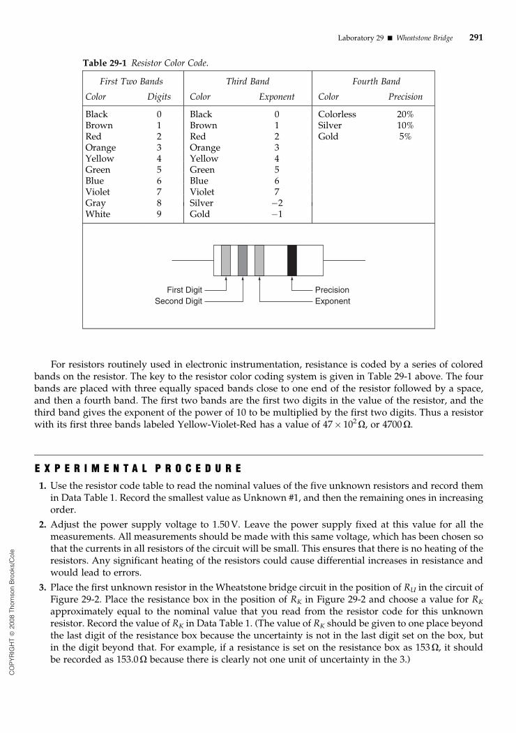
For resistors routinely used in electronic instrumentation, resistance is coded by a series of coloredbands on the resistor. The key to the resistor color coding system is given in Table 29-1 above. The fourbands are placed with three equally spaced bands close to one end of the resistor followed by a space,and then a fourth band. The first two bands are the first two digits in the value of the resistor, and thethird band gives the exponent of the power of 10 to be multiplied by the first two digits. Thus a resistorwith its first three bands labeled Yellow-Violet-Red has a value of 47� 102O, or 4700O.
E X P E R I M E N T A L P R O C E D U R E1. Use the resistor code table to read the nominal values of the five unknown resistors and record them
in Data Table 1. Record the smallest value as Unknown #1, and then the remaining ones in increasingorder.
2. Adjust the power supply voltage to 1.50V. Leave the power supply fixed at this value for all themeasurements. All measurements should be made with this same voltage, which has been chosen sothat the currents in all resistors of the circuit will be small. This ensures that there is no heating of theresistors. Any significant heating of the resistors could cause differential increases in resistance andwould lead to errors.
3. Place the first unknown resistor in the Wheatstone bridge circuit in the position of RU in the circuit ofFigure 29-2. Place the resistance box in the position of RK in Figure 29-2 and choose a value for RK
approximately equal to the nominal value that you read from the resistor code for this unknownresistor. Record the value of RK in Data Table 1. (The value of RK should be given to one place beyondthe last digit of the resistance box because the uncertainty is not in the last digit set on the box, butin the digit beyond that. For example, if a resistance is set on the resistance box as 153O, it shouldbe recorded as 153.0O because there is clearly not one unit of uncertainty in the 3.)
COPYRIG
HTª
2008ThomsonBrooks/Cole
Table 29-1 Resistor Color Code.
First Two Bands Third Band Fourth Band
Color Digits Color Exponent Color Precision
Black 0 Black 0 Colorless 20%Brown 1 Brown 1 Silver 10%Red 2 Red 2 Gold 5%Orange 3 Orange 3Yellow 4 Yellow 4Green 5 Green 5Blue 6 Blue 6Violet 7 Violet 7Gray 8 Silver �2White 9 Gold �1
PrecisionExponent
First DigitSecond Digit
Laboratory 29 n Wheatstone Bridge 291

4. The 10 kO resistor and switch S in series with the galvanometer are designed to protect thegalvanometer from excessive current. Be sure that each attempt to find a balance condition starts withswitch S open. This places the resistor in series with the galvanometer and limits the current.
5. With switch S open, move the sliding contact at B until a balance is achieved—i.e., zero current in thegalvanometer. This is a rough balance.
6. With the system at rough balance, close switch S to achieve maximum sensitivity at the final balancecondition. Balance is the point where there is no deflection of the meter, which may not be at zero ofthe meter if the galvanometer has a zero offset. Record in Data Table 1 the values of JB and BK, thelength of the two sections of wire at balance. The Wheatstone bridge has 1mm as the smallest markeddivision. Therefore, measurements of JB and BK should be made to the nearest 0.1mm.
7. Using the same unknown resistor, repeat Steps 3 through 6 above with two other values of RK, onevalue approximately 10% greater than the original RK, and one value approximately 10% less than theoriginal RK.
8. Repeat Steps 3 through 7 for each of the other four unknown resistors.
9. Use the resistance scale on a multimeter to measure the value of each of the five unknown resistorsand record those values in Data Table 2.
C A L C U L A T I O N S1. Calculate and record the three measured values for each of the five unknown resistors in the
Calculations Table.
2. Calculate and record the mean and standard error for the three measurements of each of the fiveresistors.
292 Physics Laboratory Manual n Loyd
Name . . . . . . . . . . . . . . . . . . . . . . . . . . . . . . . . . . . . . . . . . . . . . . . . . . . . . . . . . . . . . . . . . . . . . . . . . Section . . . . . . . . . . . . . . . . Date . . . . . . . . . . . . . . . .
29 L A B O R A T O R Y 2 9 Wheatstone Bridge
P R E - L A B O R A T O R Y A S S I G N M E N T1. When the Wheatstone bridge in Figure 29-1 is balanced, which of the following statements are true?
(More than one may be true.) (a) There is no current in the unknown resistor. (b) There is no current inthe galvanometer. (c) There is no voltage drop across the galvanometer. (d) The currents in R1 and R3
are the same. (e) The currents in R1 and R2 are the same. (f) The voltage across R1 and R3 is the same.(g) The voltage across R1 and R2 is the same.
2. The slide-wire form of the Wheatstone bridge makes use of the fact that (a) the resistance of a wire isequal to its length (b) the resistance of a wire is proportional to its cross-sectional area (c) the resistanceof a wire is proportional to its length (d) the resistance of a wire is inversely proportional to its length.
3. A slide-wire Wheatstone bridge is used in the configuration shown in Figure 29-2 with the knownresistor positioned as shown and equal to 10.00O. The balance point is found to be at the positionof 35.7 cm for the scale as shown in the figure. What is the value of the unknown resistance RU?Show your work.
RU ¼ �
4. Does the measurement of resistance using the Wheatstone bridge depend upon the value of thepower supply voltage used? If it does, explain why, and if it does not, then explain why not.
5. What is the purpose of the 10 kO resistor in parallel with the switch that is in series with thegalvanometer in Figure 29-2?
COPYRIG
HTª
2008ThomsonBrooks/Cole
293

6. A resistor is coded as shown below. What is the nominal value of the resistor, and what is theprecision of this value?
Green
Blue
Orange
Silver
294 Physics Laboratory Manual n Loyd

Name . . . . . . . . . . . . . . . . . . . . . . . . . . . . . . . . . . . . . . . . . . . . . . . . . . . . . . . . . . . . . . . . . . . . . . . . . Section . . . . . . . . . . . . . . . . Date . . . . . . . . . . . . . . . .
Lab Partners . . . . . . . . . . . . . . . . . . . . . . . . . . . . . . . . . . . . . . . . . . . . . . . . . . . . . . . . . . . . . . . . . . . . . . . . . . . . . . . . . . . . . . . . . . . . . . . . . . . . . . . . . . . . . . . . . . . .
29 L A B O R A T O R Y 2 9 Wheatstone Bridge
L A B O R A T O R Y R E P O R T
COPYRIG
HTª
2008ThomsonBrooks/Cole
Data Table 1
RK (O) JB (cm) BK (cm)
Unknown #1
Coded Value
( O)
Unknown #2
Coded Value
( O)
Unknown #3
Coded Value
( O)
Unknown #4
Coded Value
( O)
Unknown #5
Coded Value
( O)
Calculations Table 1
RU (O) RU (O) aRU (O)
295
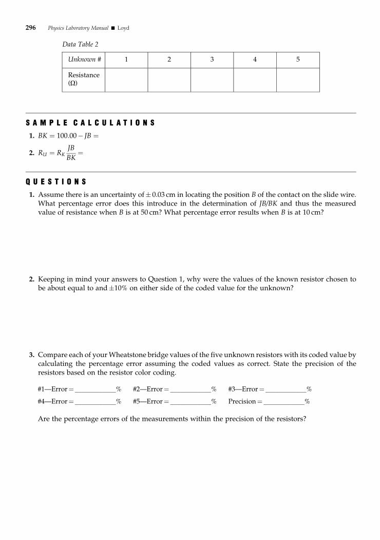
S A M P L E C A L C U L A T I O N S1. BK ¼ 100:00� JB ¼
2. RU ¼ RKJB
BK¼
Q U E S T I O N S1. Assume there is an uncertainty of� 0.03 cm in locating the position B of the contact on the slide wire.
What percentage error does this introduce in the determination of JB/BK and thus the measuredvalue of resistance when B is at 50 cm? What percentage error results when B is at 10 cm?
2. Keeping in mind your answers to Question 1, why were the values of the known resistor chosen tobe about equal to and�10% on either side of the coded value for the unknown?
3. Compare each of yourWheatstone bridge values of the five unknown resistors with its coded value bycalculating the percentage error assuming the coded values as correct. State the precision of theresistors based on the resistor color coding.
#1—Error¼ ____________% #2—Error¼ ____________% #3—Error¼ ____________%
#4—Error¼ ____________% #5—Error¼ ____________% Precision¼ ____________%
Are the percentage errors of the measurements within the precision of the resistors?
Data Table 2
Unknown # 1 2 3 4 5
Resistance(O)
296 Physics Laboratory Manual n Loyd
4. Compare yourWheatstone bridge values of the five unknown resistors with the values in Data Table 2determined by using the resistance meter. Calculate the percentage errors for each resistor assumingData Table 2 as correct. For each resistor, is the agreement better or worse than the agreement with thecoded values?
#1—Error¼ ____________% #2—Error¼ ____________% #3—Error¼ ____________%
#4—Error¼ ____________% #5—Error¼ ____________%
5. Express the values of the standard error for each of the five unknown resistors as a percentage of themean value.
#1 % std err¼ ____________% #2 % std err¼ ____________% #3 % std err¼ ____________%
#4 % std err¼ ____________% #5 % std err¼ ____________%
6. Considering the stated precision of the coded values and the various comparisons that have beendone above, state whether or not your Wheatstone bridge measurements of these resistors representmore reliable values for the actual values of these resistors than the coded values. Be very specificabout the facts upon which your opinion is based.
COPYRIG
HTª
2008ThomsonBrooks/Cole
Laboratory 29 n Wheatstone Bridge 297

This page intentionally left blank

Bridge Measurementof Capacitance
O B J E C T I V E So Determine the capacitance of several unknown capacitors by establishing balance in a bridge
circuit.
o Experimentally determine the capacitance of series and parallel combinations of capacitors andcompare the results with theoretical predictions.
E Q U I P M E N T L I S T. Capacitor of accurately known value (in the range 0.5–1mF). Three capacitors of unknown value (in the range 0.2–3mF). Two decade resistance boxes (1000O and 10,000O). Sine wave generator (variable frequency, 5V peak to peak amplitude)
. Alternating current voltmeter (digital readout, capable of measuring high frequency)
T H E O R YA capacitor is a circuit element that consists of two conducting surfaces separated by an insulatingmaterial called a dielectric. When an alternating current of frequency f exists in a capacitor, the measure ofopposition to that current is a quantity called the capacitive reactance XC. The potential difference acrossthe capacitor is given by IXC where I is the current in the capacitor. Thus XC plays a role for alternatingcurrent that is analogous to the role played by resistors for direct current. This quantity depends on theangular frequency o¼ 2pf and on the capacitance C and is given by XC¼ 1/oC. In this laboratory we willconstruct an alternating current bridge circuit with two capacitors and two resistors. When the bridge isbalanced, the ratio of the value of the two capacitive reactances is equal to the ratio of the value of the tworesistors. If the value of the ratio of the resistors and the value of one capacitor is known, the capacitance ofthe other capacitor can be determined.
Consider the circuit shown in Figure 30-1, which is a form of alternating current bridge. A capacitor ofunknown value CU and a capacitor of known value CK are in the circuit along with resistors R1 and R2.A sine wave generator is applied between points A andD in the circuit. If an alternating current voltmeterbetween points B and C reads zero, the bridge is balanced and VBC¼ 0. If VBC is zero, then points B and Care at the same potential, and that means that the potential difference VAB between points A and B is the
Physics Laboratory Manual n Loyd L A B O R A T O R Y 30
COPYRIG
HTª
2008ThomsonBrooks/Cole
299
ª 2008 Thomson Brooks/Cole, a part of TheThomson Corporation.Thomson, the Star logo, and Brooks/Cole are trademarks used herein under license. ALL RIGHTSRESERVED.No part of this workcovered by the copyright hereonmay be reproduced or used in any form or by any meansçgraphic, electronic, ormechanical, including photocopying, recording, taping,web distribution, informationstorage and retrieval systems,or in any othermannerçwithout the written permission of the publisher.
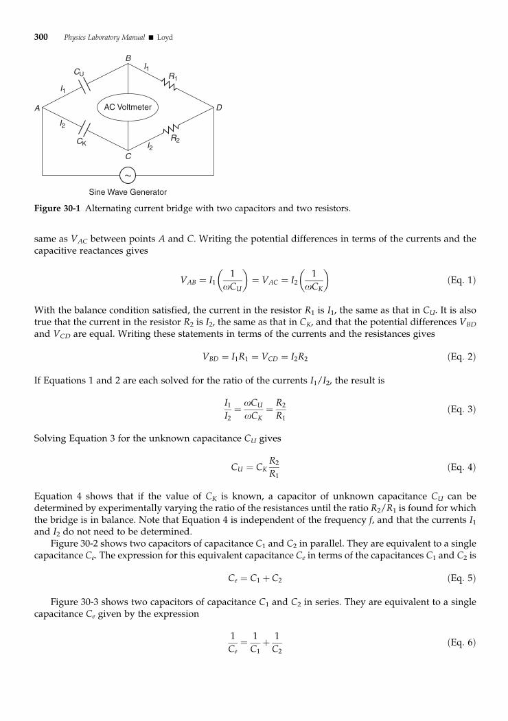
same as VAC between points A and C. Writing the potential differences in terms of the currents and thecapacitive reactances gives
VAB ¼ I11
oCU
� ¼ VAC ¼ I2
1
oCK
� ðEq: 1Þ
With the balance condition satisfied, the current in the resistor R1 is I1, the same as that in CU. It is alsotrue that the current in the resistor R2 is I2, the same as that in CK, and that the potential differences VBD
and VCD are equal. Writing these statements in terms of the currents and the resistances gives
VBD ¼ I1R1 ¼ VCD ¼ I2R2 ðEq: 2Þ
If Equations 1 and 2 are each solved for the ratio of the currents I1/I2, the result is
I1I2
¼ oCU
oCK¼ R2
R1ðEq: 3Þ
Solving Equation 3 for the unknown capacitance CU gives
CU ¼ CKR2
R1ðEq: 4Þ
Equation 4 shows that if the value of CK is known, a capacitor of unknown capacitance CU can bedetermined by experimentally varying the ratio of the resistances until the ratio R2/R1 is found for whichthe bridge is in balance. Note that Equation 4 is independent of the frequency f, and that the currents I1and I2 do not need to be determined.
Figure 30-2 shows two capacitors of capacitance C1 and C2 in parallel. They are equivalent to a singlecapacitance Ce. The expression for this equivalent capacitance Ce in terms of the capacitances C1 and C2 is
Ce ¼ C1 þ C2 ðEq: 5Þ
Figure 30-3 shows two capacitors of capacitance C1 and C2 in series. They are equivalent to a singlecapacitance Ce given by the expression
1
Ce¼ 1
C1þ 1
C2ðEq: 6Þ
CU
I1
I2
I1
I2CK
R1
B
A D
C
Sine Wave Generator
AC Voltmeter
R2
Figure 30-1 Alternating current bridge with two capacitors and two resistors.
300 Physics Laboratory Manual n Loyd
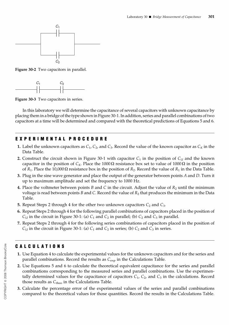
In this laboratory wewill determine the capacitance of several capacitors with unknown capacitance byplacing them ina bridgeof the type shown inFigure 30-1. In addition, series andparallel combinations of twocapacitors at a time will be determined and compared with the theoretical predictions of Equations 5 and 6.
E X P E R I M E N T A L P R O C E D U R E1. Label the unknown capacitors as C1, C2, and C3. Record the value of the known capacitor as CK in the
Data Table.
2. Construct the circuit shown in Figure 30-1 with capacitor C1 in the position of CU and the knowncapacitor in the position of CK. Place the 1000O resistance box set to value of 1000O in the positionof R1. Place the 10,000O resistance box in the position of R2. Record the value of R1 in the Data Table.
3. Plug in the sine wave generator and place the output of the generator between points A andD. Turn itup to maximum amplitude and set the frequency to 1000 Hz.
4. Place the voltmeter between points B and C in the circuit. Adjust the value of R2 until the minimumvoltage is read between points B and C. Record the value of R2 that produces the minimum in the DataTable.
5. Repeat Steps 2 through 4 for the other two unknown capacitors C2 and C3.
6. Repeat Steps 2 through 4 for the following parallel combinations of capacitors placed in the position ofCU in the circuit in Figure 30-1: (a) C1 and C2 in parallel; (b) C2 and C3 in parallel.
7. Repeat Steps 2 through 4 for the following series combinations of capacitors placed in the position ofCU in the circuit in Figure 30-1: (a) C1 and C2 in series; (b) C2 and C3 in series.
C A L C U L A T I O N S1. Use Equation 4 to calculate the experimental values for the unknown capacitors and for the series and
parallel combinations. Record the results as Cexp in the Calculations Table.
2. Use Equations 5 and 6 to calculate the theoretical equivalent capacitance for the series and parallelcombinations corresponding to the measured series and parallel combinations. Use the experimen-tally determined values for the capacitance of capacitors C1, C2, and C3 in the calculations. Recordthose results as Ctheo in the Calculations Table.
3. Calculate the percentage error of the experimental values of the series and parallel combinationscompared to the theoretical values for those quantities. Record the results in the Calculations Table.
COPYRIG
HTª
2008ThomsonBrooks/Cole
C1
C2
Figure 30-2 Two capacitors in parallel.
C1 C2
Figure 30-3 Two capacitors in series.
Laboratory 30 n Bridge Measurement of Capacitance 301

This page intentionally left blank
Name . . . . . . . . . . . . . . . . . . . . . . . . . . . . . . . . . . . . . . . . . . . . . . . . . . . . . . . . . . . . . . . . . . . . . . . . . Section . . . . . . . . . . . . . . . . Date . . . . . . . . . . . . . . . .
30 L A B O R A T O R Y 3 0 Bridge Measurement of Capacitance
P R E - L A B O R A T O R Y A S S I G N M E N T1. Define capacitive reactance.
2. Describe the role that capacitive reactance of a capacitor plays when there is an alternating current inthe capacitor.
Consider the circuit diagram of Figure 30-1 for Questions 3–7. Mark as true or false the statements
concerning the conditions that hold when the bridge is balanced.
3. VAB¼VBD and VAC¼VCD (a) true (b) false
4. VBC¼ 0 (a) true (b) false
5. VAB¼VCD and VAC¼VBD (a) true (b) false
6. VAB¼VAC and VBD¼VCD (a) true (b) false
7. The balance condition for the bridge is different for different frequencies. (a) true (b) false
COPYRIG
HTª
2008ThomsonBrooks/Cole
303

8. A bridge like the one shown in Figure 30-1 is balanced. The known capacitor CK has a capacitanceof 1.17mF. The value of R1 is 1000O, and the value of R2 is 525O. What is the value of the unknowncapacitor CU? Show your work.
9. A 3.75mF capacitor is in series with a 6.85mF capacitor. What is the equivalent capacitance Ce of thecombination? Show your work.
10. A 5.75 mF capacitor is in parallel with a 3.82 mF capacitor. What is the equivalent capacitance Ce of thecombination? Show your work.
304 Physics Laboratory Manual n Loyd
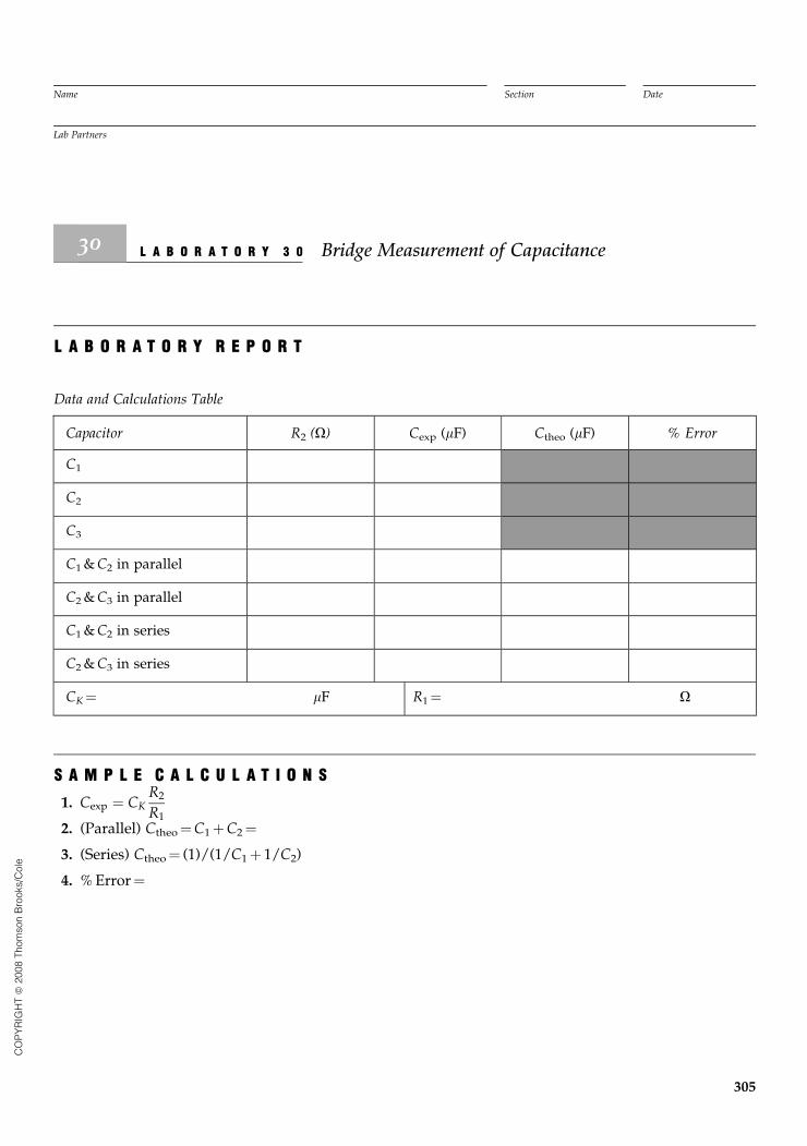
Name . . . . . . . . . . . . . . . . . . . . . . . . . . . . . . . . . . . . . . . . . . . . . . . . . . . . . . . . . . . . . . . . . . . . . . . . . Section . . . . . . . . . . . . . . . . Date . . . . . . . . . . . . . . . .
Lab Partners . . . . . . . . . . . . . . . . . . . . . . . . . . . . . . . . . . . . . . . . . . . . . . . . . . . . . . . . . . . . . . . . . . . . . . . . . . . . . . . . . . . . . . . . . . . . . . . . . . . . . . . . . . . . . . . . . . . .
30 L A B O R A T O R Y 3 0 Bridge Measurement of Capacitance
L A B O R A T O R Y R E P O R T
S A M P L E C A L C U L A T I O N S1. Cexp ¼ CK
R2
R12. (Parallel) Ctheo¼C1þC2¼3. (Series) Ctheo¼ (1)/(1/C1þ 1/C2)
4. %Error¼
COPYRIG
HTª
2008ThomsonBrooks/Cole
Data and Calculations Table
Capacitor R2 (O) Cexp (mF) Ctheo (mF) % Error
C1
C2
C3
C1&C2 in parallel
C2&C3 in parallel
C1&C2 in series
C2&C3 in series
CK¼ mF R1¼ O
305

Q U E S T I O N S1. To what extent do your data confirm the theoretical equation for the parallel combination of
capacitors? State your answer as quantitatively as possible.
2. To what extent do your data confirm the theoretical equation for the series combination of capacitors?State your answer as quantitatively as possible.
3. The laboratory procedure instructs you to use the maximum amplitude of the sine wave generator.How would it affect the results if one-half the amplitude were used instead?
4. Suppose the bridge is rearranged into the form shown in Figure 30-4. What is the balance condition forthis bridge?
5. Your lab instructor may have accurate values for your unknown capacitors or perhaps can makeavailable to you a capacitance meter that will allow you to obtain a value for them. If you can obtain areliable value for thecapacitanceof theunknowns, calculate thepercentage error inyourmeasurements.
CU
R1
CK
B
A D
C
Sine Wave Generator
R2
AC Voltmeter
Figure 30-4 Different arrangement of the alternating current bridge.
306 Physics Laboratory Manual n Loyd

Voltmeters and Ammeters
O B J E C T I V E So Determine the internal resistance Rg and current sensitivity K of a galvanometer.
o Construct a voltmeter and an ammeter by placing the appropriate values of resistance in seriesand parallel with the galvanometer.
o Compare the accuracy of the constructed voltmeter and ammeter with a standard voltmeter anda standard ammeter.
E Q U I P M E N T L I S T. Power supply (0–20V direct current), galvanometer (D’Arsonal type, zero centered)
. Resistance box (variable in steps of 10O between 2500O and 3500O)
. A resistor of about 330O (either a 1% resistor or provide a resistance meter)
. Digital voltmeter (0–20V direct current), digital ammeter (0–1.00A direct current)
. Spool of #28 copper wire (one for the class), assorted leads
T H E O R YGalvanometer Characteristics
TheD’Arsonal galvanometers used in this laboratory are based upon the fact that a wire coil in the presenceof a magnetic field experiences a torque when there is a current in the coil. This torque is exerted against aspring, and the deflection of a pointer attached to the coil is proportional to the current in the galvanometer.
Because the coil has a fixed resistance Rg, the deflection of the pointer will also be proportional to thevoltage across the terminals of the galvanometer. Therefore, a galvanometer can be calibrated to serve aseither a voltmeter or an ammeter.
A galvanometer is characterized by its resistance Rg and a constant K called the current sensitivity. K isthe amount of current needed to deflect the galvanometer one scale division. It is expressed in units ofA/div.BothRg andK are taken to beunknown for the galvanometers used in the laboratory.Wewill determine themby a series of measurements described in a later section.
Conversion of the Galvanometer into a Voltmeter
The galvanometer deflects full scale for a value of current given by Ig¼KN where N is the number of scaledivisions. The voltage Vg across the galvanometer terminals that produces a full-scale deflection is givenby Vg¼ Ig Rg¼KN Rg. If it is desired to measure a larger voltage than Vg, it is necessary to place a resistorRV in series with the galvanometer so that most of the voltage is across RV and the rest across the galvano-meter. Figure 31-1 illustrates this idea.
Physics Laboratory Manual n Loyd L A B O R A T O R Y 31
COPYRIG
HTª
2008ThomsonBrooks/Cole
307
ª 2008 Thomson Brooks/Cole, a part of TheThomson Corporation.Thomson, the Star logo, and Brooks/Cole are trademarks used herein under license. ALL RIGHTSRESERVED.No part of this workcovered by the copyright hereonmay be reproduced or used in any form or by any meansçgraphic, electronic, ormechanical, including photocopying, recording, taping,web distribution, informationstorage and retrieval systems,or in any othermannerçwithout the written permission of the publisher.
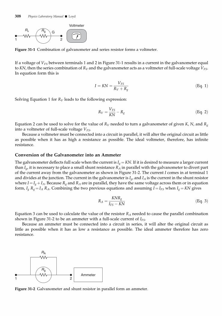
If a voltage of VFS between terminals 1 and 2 in Figure 31-1 results in a current in the galvanometer equalto KN, then the series combination of RV and the galvanometer acts as a voltmeter of full-scale voltageVFS.In equation form this is
I ¼ KN ¼ VFS
RV þ RgðEq: 1Þ
Solving Equation 1 for RV leads to the following expression:
RV ¼ VFS
KN� Rg ðEq: 2Þ
Equation 2 can be used to solve for the value of RV needed to turn a galvanometer of given K, N, and Rg
into a voltmeter of full-scale voltage VFS.Because a voltmeter must be connected into a circuit in parallel, it will alter the original circuit as little
as possible when it has as high a resistance as possible. The ideal voltmeter, therefore, has infiniteresistance.
Conversion of the Galvanometer into an Ammeter
The galvanometer deflects full scale when the current is Ig¼KN. If it is desired to measure a larger currentthan Ig, it is necessary to place a small shunt resistance RA in parallel with the galvanometer to divert partof the current away from the galvanometer as shown in Figure 31-2. The current I comes in at terminal 1and divides at the junction. The current in the galvanometer is Ig, and IA is the current in the shunt resistorwhere I¼ Igþ IA. Because Rg and RA are in parallel, they have the same voltage across them or in equationform, Ig Rg¼ IA RA. Combining the two previous equations and assuming I¼ IFS when Ig¼KN gives
RA ¼ KNRg
IFS � KNðEq: 3Þ
Equation 3 can be used to calculate the value of the resistor RA needed to cause the parallel combinationshown in Figure 31-2 to be an ammeter with a full-scale current of IFS.
Because an ammeter must be connected into a circuit in series, it will alter the original circuit aslittle as possible when it has as low a resistance as possible. The ideal ammeter therefore has zeroresistance.
GRgRv
1 2
Voltmeter
Figure 31-1 Combination of galvanometer and series resistor forms a voltmeter.
Rg
1 2Ammeter
RA
Figure 31-2 Galvanometer and shunt resistor in parallel form an ammeter.
308 Physics Laboratory Manual n Loyd
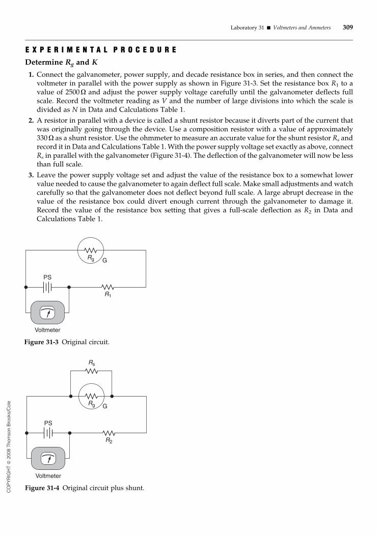
E X P E R I M E N T A L P R O C E D U R EDetermine Rg and K
1. Connect the galvanometer, power supply, and decade resistance box in series, and then connect thevoltmeter in parallel with the power supply as shown in Figure 31-3. Set the resistance box R1 to avalue of 2500O and adjust the power supply voltage carefully until the galvanometer deflects fullscale. Record the voltmeter reading as V and the number of large divisions into which the scale isdivided as N in Data and Calculations Table 1.
2. A resistor in parallel with a device is called a shunt resistor because it diverts part of the current thatwas originally going through the device. Use a composition resistor with a value of approximately330O as a shunt resistor. Use the ohmmeter to measure an accurate value for the shunt resistor Rs andrecord it in Data and Calculations Table 1.With the power supply voltage set exactly as above, connectRs in parallel with the galvanometer (Figure 31-4). The deflection of the galvanometer will now be lessthan full scale.
3. Leave the power supply voltage set and adjust the value of the resistance box to a somewhat lowervalue needed to cause the galvanometer to again deflect full scale. Make small adjustments and watchcarefully so that the galvanometer does not deflect beyond full scale. A large abrupt decrease in thevalue of the resistance box could divert enough current through the galvanometer to damage it.Record the value of the resistance box setting that gives a full-scale deflection as R2 in Data andCalculations Table 1.
COPYRIG
HTª
2008ThomsonBrooks/Cole
PS
G
Voltmeter
R1
Rg
Figure 31-3 Original circuit.
G
R2
Rg
Rs
PS
Voltmeter
Figure 31-4 Original circuit plus shunt.
Laboratory 31 n Voltmeters and Ammeters 309
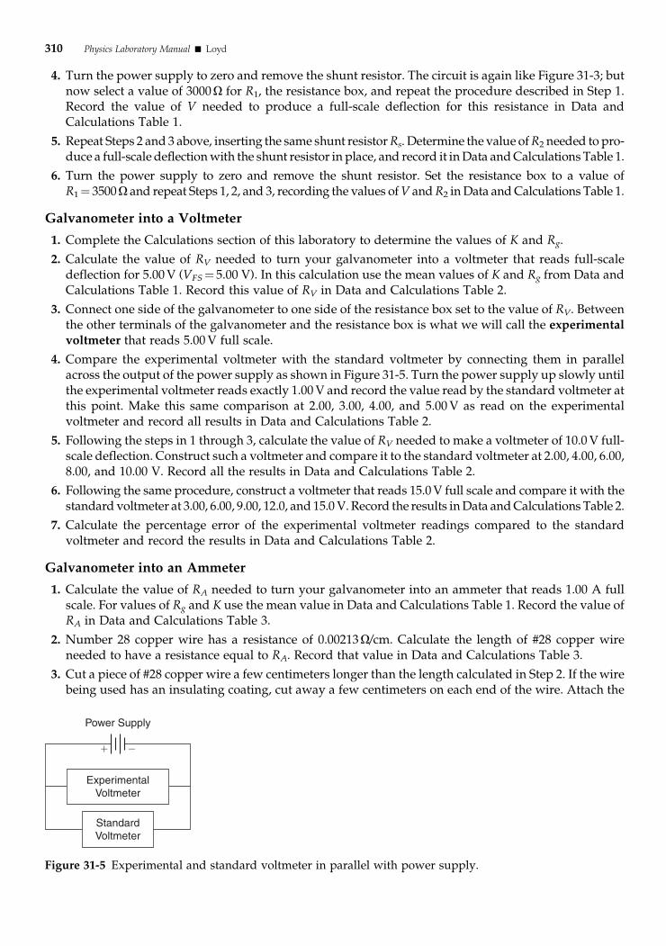
4. Turn the power supply to zero and remove the shunt resistor. The circuit is again like Figure 31-3; butnow select a value of 3000O for R1, the resistance box, and repeat the procedure described in Step 1.Record the value of V needed to produce a full-scale deflection for this resistance in Data andCalculations Table 1.
5. Repeat Steps 2 and 3 above, inserting the same shunt resistorRs. Determine the value ofR2 needed to pro-duce a full-scale deflectionwith the shunt resistor in place, and record it inData andCalculations Table 1.
6. Turn the power supply to zero and remove the shunt resistor. Set the resistance box to a value ofR1¼ 3500O and repeat Steps 1, 2, and 3, recording the values ofV andR2 inData andCalculations Table 1.
Galvanometer into a Voltmeter
1. Complete the Calculations section of this laboratory to determine the values of K and Rg.
2. Calculate the value of RV needed to turn your galvanometer into a voltmeter that reads full-scaledeflection for 5.00V (VFS¼ 5.00 V). In this calculation use the mean values of K and Rg from Data andCalculations Table 1. Record this value of RV in Data and Calculations Table 2.
3. Connect one side of the galvanometer to one side of the resistance box set to the value of RV. Betweenthe other terminals of the galvanometer and the resistance box is what we will call the experimentalvoltmeter that reads 5.00V full scale.
4. Compare the experimental voltmeter with the standard voltmeter by connecting them in parallelacross the output of the power supply as shown in Figure 31-5. Turn the power supply up slowly untilthe experimental voltmeter reads exactly 1.00V and record the value read by the standard voltmeter atthis point. Make this same comparison at 2.00, 3.00, 4.00, and 5.00V as read on the experimentalvoltmeter and record all results in Data and Calculations Table 2.
5. Following the steps in 1 through 3, calculate the value of RV needed to make a voltmeter of 10.0V full-scale deflection. Construct such a voltmeter and compare it to the standard voltmeter at 2.00, 4.00, 6.00,8.00, and 10.00 V. Record all the results in Data and Calculations Table 2.
6. Following the same procedure, construct a voltmeter that reads 15.0V full scale and compare it with thestandard voltmeter at 3.00, 6.00, 9.00, 12.0, and15.0V.Record the results inData andCalculations Table 2.
7. Calculate the percentage error of the experimental voltmeter readings compared to the standardvoltmeter and record the results in Data and Calculations Table 2.
Galvanometer into an Ammeter
1. Calculate the value of RA needed to turn your galvanometer into an ammeter that reads 1.00 A fullscale. For values of Rg and K use the mean value in Data and Calculations Table 1. Record the value ofRA in Data and Calculations Table 3.
2. Number 28 copper wire has a resistance of 0.00213O/cm. Calculate the length of #28 copper wireneeded to have a resistance equal to RA. Record that value in Data and Calculations Table 3.
3. Cut a piece of #28 copper wire a few centimeters longer than the length calculated in Step 2. If the wirebeing used has an insulating coating, cut away a few centimeters on each end of the wire. Attach the
ExperimentalVoltmeter
Power Supply
� �
StandardVoltmeter
Figure 31-5 Experimental and standard voltmeter in parallel with power supply.
310 Physics Laboratory Manual n Loyd
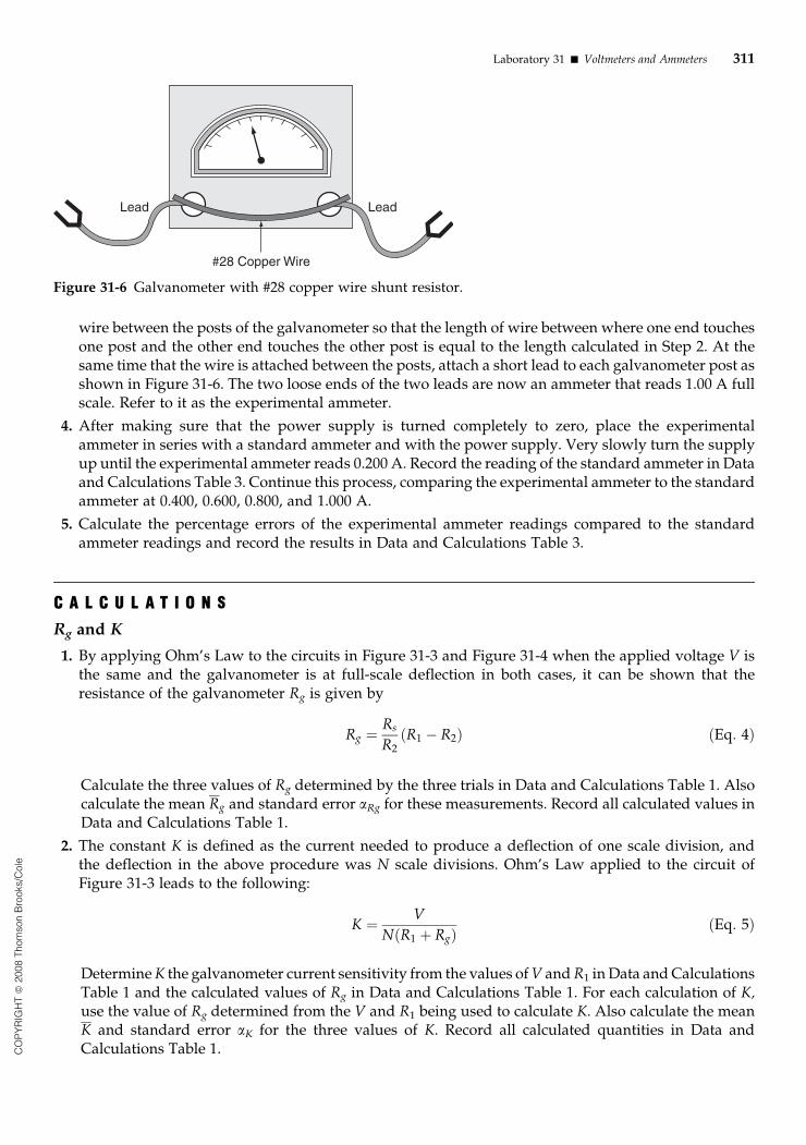
wire between the posts of the galvanometer so that the length of wire between where one end touchesone post and the other end touches the other post is equal to the length calculated in Step 2. At thesame time that the wire is attached between the posts, attach a short lead to each galvanometer post asshown in Figure 31-6. The two loose ends of the two leads are now an ammeter that reads 1.00 A fullscale. Refer to it as the experimental ammeter.
4. After making sure that the power supply is turned completely to zero, place the experimentalammeter in series with a standard ammeter and with the power supply. Very slowly turn the supplyup until the experimental ammeter reads 0.200 A. Record the reading of the standard ammeter in Dataand Calculations Table 3. Continue this process, comparing the experimental ammeter to the standardammeter at 0.400, 0.600, 0.800, and 1.000 A.
5. Calculate the percentage errors of the experimental ammeter readings compared to the standardammeter readings and record the results in Data and Calculations Table 3.
C A L C U L A T I O N SRg and K
1. By applying Ohm’s Law to the circuits in Figure 31-3 and Figure 31-4 when the applied voltage V isthe same and the galvanometer is at full-scale deflection in both cases, it can be shown that theresistance of the galvanometer Rg is given by
Rg ¼ Rs
R2ðR1 � R2Þ ðEq: 4Þ
Calculate the three values of Rg determined by the three trials in Data and Calculations Table 1. Alsocalculate the mean Rg and standard error aRg for these measurements. Record all calculated values inData and Calculations Table 1.
2. The constant K is defined as the current needed to produce a deflection of one scale division, andthe deflection in the above procedure was N scale divisions. Ohm’s Law applied to the circuit ofFigure 31-3 leads to the following:
K ¼ V
NðR1 þ RgÞ ðEq: 5Þ
DetermineK the galvanometer current sensitivity from the values ofV andR1 in Data andCalculationsTable 1 and the calculated values of Rg in Data and Calculations Table 1. For each calculation of K,use the value of Rg determined from the V and R1 being used to calculate K. Also calculate the meanK and standard error aK for the three values of K. Record all calculated quantities in Data andCalculations Table 1.C
OPYRIG
HTª
2008ThomsonBrooks/Cole
#28 Copper Wire
LeadLead
Figure 31-6 Galvanometer with #28 copper wire shunt resistor.
Laboratory 31 n Voltmeters and Ammeters 311

This page intentionally left blank

Name . . . . . . . . . . . . . . . . . . . . . . . . . . . . . . . . . . . . . . . . . . . . . . . . . . . . . . . . . . . . . . . . . . . . . . . . . Section . . . . . . . . . . . . . . . . Date . . . . . . . . . . . . . . . .
31 L A B O R A T O R Y 3 1 Voltmeters and Ammeters
P R E - L A B O R A T O R Y A S S I G N M E N T1. Describe the principle on which the operation of a D’Arsonal type galvanometer is based.
2. A galvanometer has (a) a meter deflection proportional to the current in the galvanometer (b) a meterdeflection proportional to the voltage across the galvanometer (c) a fixed resistance (d) all of the aboveare true.
3. The galvanometer constant K is (a) the current for full-scale deflection (units A) (b) the current fordeflection of one scale division (units A/div) (c) the total current times the number of scale divisions(units A/div) (d) the reciprocal of the galvanometer resistance Rg (units 1/A).
4. In the procedure for determination of Rg and K when the shunt resistor RS is placed in parallel withthe galvanometer, what happens to galvanometer deflection, and why does it happen?
5. To construct a voltmeter of a given full-scale deflection from a galvanometer, the appropriate resis-tance must be placed in (a) series (b) parallel with the galvanometer.
6. To construct an ammeter of a given full-scale deflection from a galvanometer, the appropriate resis-tance must be placed in (a) series (b) parallel with the galvanometer.
COPYRIG
HTª
2008ThomsonBrooks/Cole
313

7. A galvanometer has Rg¼ 150O and K¼ 0.750� 10�4 A/div. The galvanometer has five divisions fora full-scale reading (i.e., N¼ 5). What value of resistance is needed, and how must it be connected tothe galvanometer to form a full-scale voltmeter of 20.0 V? Show your work.
8. To form the galvanometer of Question 7 into an ammeter of 2.50 A full scale, what value of resistanceis needed, and how must it be connected? Show your work.
9. Tomeasure voltage, a voltmeter is placed in a circuit in (a) series (b) parallel. The resistance of an idealvoltmeter is ____________________.
10. To measure the current, an ammeter is placed in a circuit in (a) series (b) parallel. The resistance of anideal ammeter is ____________________.
314 Physics Laboratory Manual n Loyd

Name . . . . . . . . . . . . . . . . . . . . . . . . . . . . . . . . . . . . . . . . . . . . . . . . . . . . . . . . . . . . . . . . . . . . . . . . . Section . . . . . . . . . . . . . . . . Date . . . . . . . . . . . . . . . .
Lab Partners . . . . . . . . . . . . . . . . . . . . . . . . . . . . . . . . . . . . . . . . . . . . . . . . . . . . . . . . . . . . . . . . . . . . . . . . . . . . . . . . . . . . . . . . . . . . . . . . . . . . . . . . . . . . . . . . . . . .
31 L A B O R A T O R Y 3 1 Voltmeters and Ammeters
L A B O R A T O R Y R E P O R T
COPYRIG
HTª
2008ThomsonBrooks/Cole
Data and Calculations Table 1
R1 (O) V (V) R2 (O) Rg (O) K (A/div) Rg (O) aRg (O) K (A/div) aK (A/div)
N¼ Rs¼ O
Data and Calculations Table 2
VFS¼ 5.00 V
RV¼ O
Experimental 1.00 V 2.00V 3.00V 4.00V 5.00V
Standard V V V V V
% Error
VFS¼ 10.00 V
RV¼ O
Experimental 2.00V 4.00V 6.00V 8.00V 10.0V
Standard V V V V V
% Error
VFS¼ 15.00V
RV¼ O
Experimental 3.00V 6.00V 9.00V 12.0V 15.0V
Standard V V V V V
% Error
315
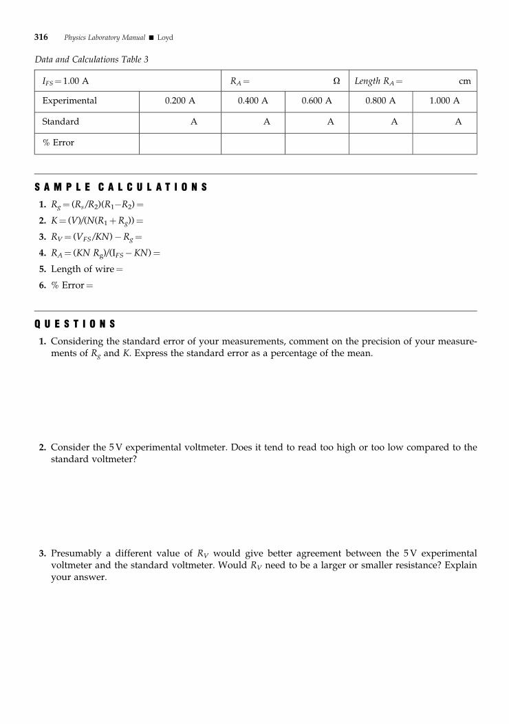
S A M P L E C A L C U L A T I O N S1. Rg¼ (Rs/R2)(R1�R2)¼2. K¼ (V)/(N(R1þRg))¼3. RV¼ (VFS/KN)�Rg¼4. RA¼ (KN Rg)/(IFS�KN)¼5. Length of wire¼6. % Error¼
Q U E S T I O N S1. Considering the standard error of your measurements, comment on the precision of your measure-
ments of Rg and K. Express the standard error as a percentage of the mean.
2. Consider the 5V experimental voltmeter. Does it tend to read too high or too low compared to thestandard voltmeter?
3. Presumably a different value of RV would give better agreement between the 5V experimentalvoltmeter and the standard voltmeter. Would RV need to be a larger or smaller resistance? Explainyour answer.
Data and Calculations Table 3
IFS¼ 1.00 A RA¼ O Length RA¼ cm
Experimental 0.200 A 0.400 A 0.600 A 0.800 A 1.000 A
Standard A A A A A
% Error
316 Physics Laboratory Manual n Loyd

4. Does the experimental ammeter tend to read too high or too low?
5. Presumably by a change in the value of RA, the experimental voltmeter could be made to show betteragreement with the standard ammeter. Does RA need to be a larger or smaller resistance to accomplishthis? Explain your answer.
EXTRA CREDIT QUESTION. It is stated in the laboratory instructions that the same voltage V isapplied to both circuits in Figure 31-3 and Figure 31-4, and that the galvanometer deflects full scale inboth cases. Thus the galvanometer current is Ig¼KN for both circuits. In Figure 31-4 let the current inRs be called Is. From the application of Ohm’s Law to these circuits, derive the expression given asEquation 1 for Rg.
COPYRIG
HTª
2008ThomsonBrooks/Cole
Laboratory 31 n Voltmeters and Ammeters 317

This page intentionally left blank
Potentiometer andVoltmeter Measurementsof the emf of a Dry Cell
O B J E C T I V E So Investigate the principles of operation of a potentiometer.
o Compare the emf of dry cells determined by a potentiometer with the emf measured bya voltmeter.
o Determine the internal resistance of a dry cell.
E Q U I P M E N T L I S T. Slide-wire potentiometer, galvanometer, standard cell
. Single-pole (single-throw) switch with a 10 kO resistor in parallel
. Single-pole (double-throw) switch, dry cells (with emfs in range 1.5 to 1.3V)
. Direct current power supply (voltage and current determined by form of potentiometer)
. Voltmeter (resistance at least 10MO), student-type voltmeter (resistance� 3 kO)
. Decade resistance box (100 kO maximum), assorted connecting leads, tap key
T H E O R YPart 1. Dry Cell Characteristics
A new dry cell produces an electromotive force (emf) between 1.50 and 1.60V with an internal resistancein the range of a fraction to a few ohms. The symbol for emf is e, and the symbol for internal resistance isRi. The voltage that appears across the dry cell terminals when the dry cell is providing current I to acircuit is called the terminal voltage V. It is given by
V ¼ e� I Ri ðEq: 1Þ
When current flows, the terminal voltage is always less than the emf of a cell by the amount of the voltagedrop across Ri. If no current is provided by the cell, its terminal voltage equals its emf (V¼ e if I¼ 0).
Physics Laboratory Manual n Loyd L A B O R A T O R Y 32
COPYRIG
HTª
2008ThomsonBrooks/Cole
319
ª 2008 Thomson Brooks/Cole, a part of TheThomson Corporation.Thomson, the Star logo, and Brooks/Cole are trademarks used herein under license. ALL RIGHTSRESERVED.No part of this workcovered by the copyright hereonmay be reproduced or used in any form or by any meansçgraphic, electronic, ormechanical, including photocopying, recording, taping,web distribution, informationstorage and retrieval systems,or in any othermannerçwithout the written permission of the publisher.
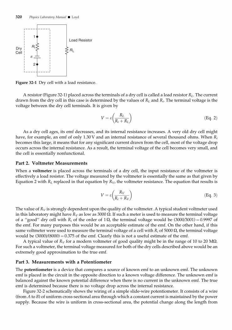
A resistor (Figure 32-1) placed across the terminals of a dry cell is called a load resistor RL. The currentdrawn from the dry cell in this case is determined by the values of RL and Ri. The terminal voltage is thevoltage between the dry cell terminals. It is given by
V ¼ eRL
Ri þ RL
� ðEq: 2Þ
As a dry cell ages, its emf decreases, and its internal resistance increases. A very old dry cell mighthave, for example, an emf of only 1.30V and an internal resistance of several thousand ohms. When Ri
becomes this large, it means that for any significant current drawn from the cell, most of the voltage dropoccurs across the internal resistance. As a result, the terminal voltage of the cell becomes very small, andthe cell is essentially nonfunctional.
Part 2. Voltmeter Measurements
When a voltmeter is placed across the terminals of a dry cell, the input resistance of the voltmeter iseffectively a load resistor. The voltage measured by the voltmeter is essentially the same as that given byEquation 2 with RL replaced in that equation by RV, the voltmeter resistance. The equation that results is
V ¼ eRV
Ri þ RV
� ðEq: 3Þ
The value of RV is strongly dependent upon the quality of the voltmeter. A typical student voltmeter usedin this laboratory might have RV as low as 3000 O. If such a meter is used to measure the terminal voltageof a ‘‘good’’ dry cell with Ri of the order of 1O, the terminal voltage would be (3000/3001)¼ 0.9997 ofthe emf. For many purposes this would be an acceptable estimate of the emf. On the other hand, if thissame voltmeter were used to measure the terminal voltage of a cell with Ri of 5000 O, the terminal voltagewould be (3000)/(8000)¼ 0.375 of the emf. Clearly this is not a useful estimate of the emf.
A typical value of RV for a modern voltmeter of good quality might be in the range of 10 to 20 MO.For such a voltmeter, the terminal voltage measured for both of the dry cells described above would be anextremely good approximation to the true emf.
Part 3. Measurements with a Potentiometer
The potentiometer is a device that compares a source of known emf to an unknown emf. The unknownemf is placed in the circuit in the opposite direction to a known voltage difference. The unknown emf isbalanced against the known potential difference when there is no current in the unknown emf. The trueemf is determined because there is no voltage drop across the internal resistance.
Figure 32-2 schematically shows the wiring of a simple slide-wire potentiometer. It consists of a wire(fromA to B) of uniform cross-sectional area throughwhich a constant current is maintained by the powersupply. Because the wire is uniform in cross-sectional area, the potential change along the length from
RL
R i
�
1Load Resistor
DryCell
2
Figure 32-1 Dry cell with a load resistance.
320 Physics Laboratory Manual n Loyd
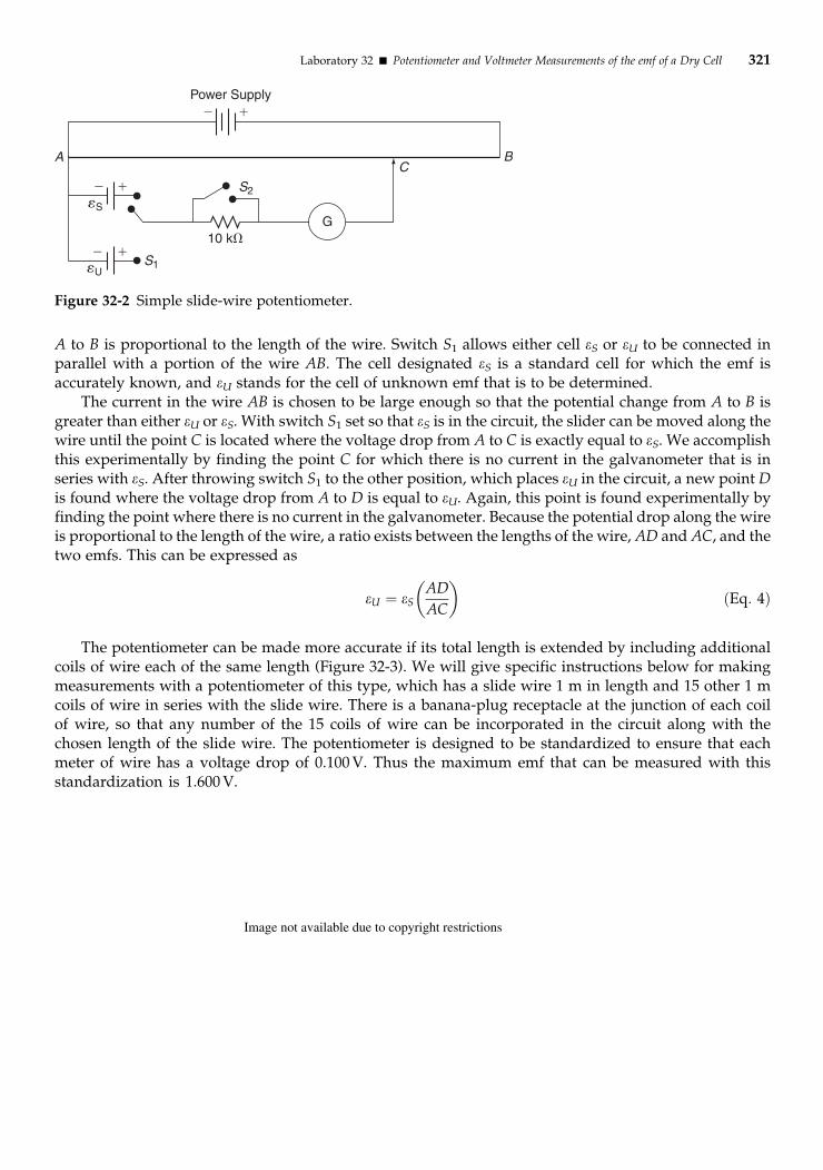
A to B is proportional to the length of the wire. Switch S1 allows either cell eS or eU to be connected inparallel with a portion of the wire AB. The cell designated eS is a standard cell for which the emf isaccurately known, and eU stands for the cell of unknown emf that is to be determined.
The current in the wire AB is chosen to be large enough so that the potential change from A to B isgreater than either eU or eS. With switch S1 set so that eS is in the circuit, the slider can be moved along thewire until the point C is located where the voltage drop from A to C is exactly equal to eS. We accomplishthis experimentally by finding the point C for which there is no current in the galvanometer that is inseries with eS. After throwing switch S1 to the other position, which places eU in the circuit, a new point Dis found where the voltage drop from A to D is equal to eU. Again, this point is found experimentally byfinding the point where there is no current in the galvanometer. Because the potential drop along the wireis proportional to the length of the wire, a ratio exists between the lengths of the wire, AD and AC, and thetwo emfs. This can be expressed as
eU ¼ eSAD
AC
� ðEq: 4Þ
The potentiometer can be made more accurate if its total length is extended by including additionalcoils of wire each of the same length (Figure 32-3). We will give specific instructions below for makingmeasurements with a potentiometer of this type, which has a slide wire 1 m in length and 15 other 1 mcoils of wire in series with the slide wire. There is a banana-plug receptacle at the junction of each coilof wire, so that any number of the 15 coils of wire can be incorporated in the circuit along with thechosen length of the slide wire. The potentiometer is designed to be standardized to ensure that eachmeter of wire has a voltage drop of 0.100V. Thus the maximum emf that can be measured with thisstandardization is 1.600V.
��
��
�U
���S
S1
S2
A
Power Supply
10 k�
BC
G
Figure 32-2 Simple slide-wire potentiometer.
Laboratory 32 n Potentiometer and Voltmeter Measurements of the emf of a Dry Cell 321
Image not available due to copyright restrictions
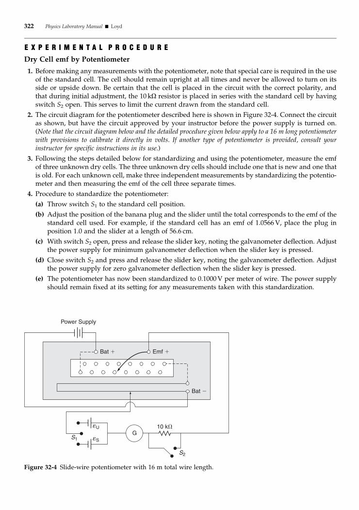
E X P E R I M E N T A L P R O C E D U R EDry Cell emf by Potentiometer
1. Before making any measurements with the potentiometer, note that special care is required in the useof the standard cell. The cell should remain upright at all times and never be allowed to turn on itsside or upside down. Be certain that the cell is placed in the circuit with the correct polarity, andthat during initial adjustment, the 10 kO resistor is placed in series with the standard cell by havingswitch S2 open. This serves to limit the current drawn from the standard cell.
2. The circuit diagram for the potentiometer described here is shown in Figure 32-4. Connect the circuitas shown, but have the circuit approved by your instructor before the power supply is turned on.(Note that the circuit diagram below and the detailed procedure given below apply to a 16 m long potentiometerwith provisions to calibrate it directly in volts. If another type of potentiometer is provided, consult yourinstructor for specific instructions in its use.)
3. Following the steps detailed below for standardizing and using the potentiometer, measure the emfof three unknown dry cells. The three unknown dry cells should include one that is new and one thatis old. For each unknown cell, make three independent measurements by standardizing the potentio-meter and then measuring the emf of the cell three separate times.
4. Procedure to standardize the potentiometer:
(a) Throw switch S1 to the standard cell position.
(b) Adjust the position of the banana plug and the slider until the total corresponds to the emf of thestandard cell used. For example, if the standard cell has an emf of 1.0566V, place the plug inposition 1.0 and the slider at a length of 56.6 cm.
(c) With switch S2 open, press and release the slider key, noting the galvanometer deflection. Adjustthe power supply for minimum galvanometer deflection when the slider key is pressed.
(d) Close switch S2 and press and release the slider key, noting the galvanometer deflection. Adjustthe power supply for zero galvanometer deflection when the slider key is pressed.
(e) The potentiometer has now been standardized to 0.1000V per meter of wire. The power supplyshould remain fixed at its setting for any measurements taken with this standardization.
�U
�S
10 k�
Bat �
Emf �Bat �
Power Supply
S2
S1G
Figure 32-4 Slide-wire potentiometer with 16 m total wire length.
322 Physics Laboratory Manual n Loyd
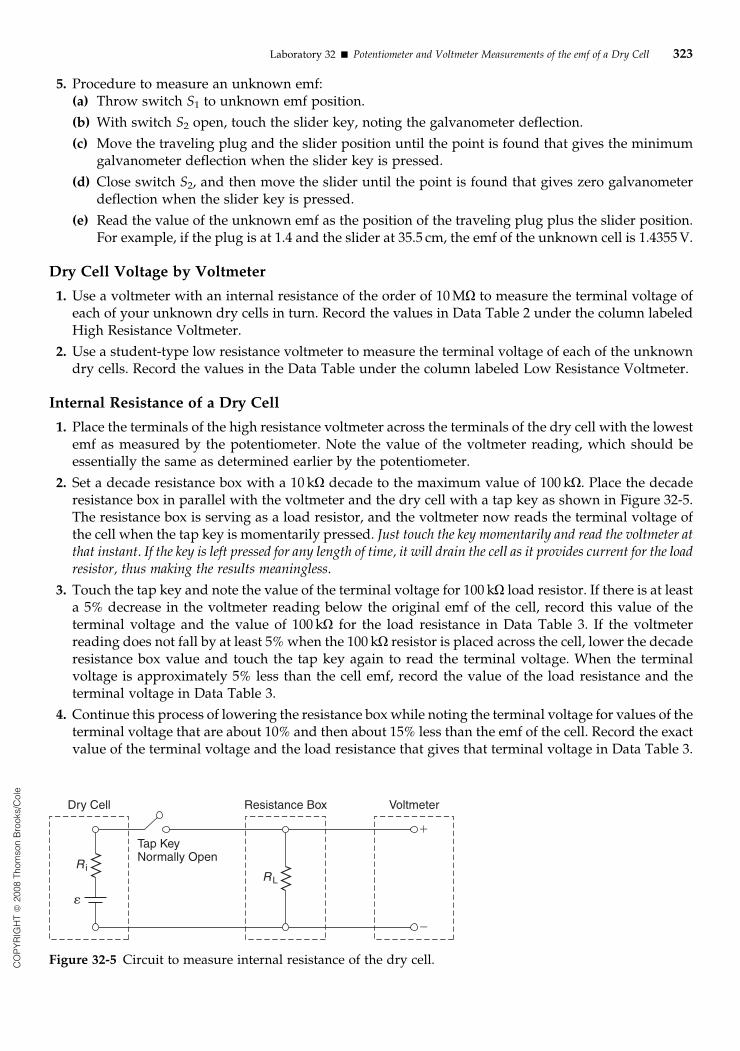
5. Procedure to measure an unknown emf:(a) Throw switch S1 to unknown emf position.
(b) With switch S2 open, touch the slider key, noting the galvanometer deflection.
(c) Move the traveling plug and the slider position until the point is found that gives the minimumgalvanometer deflection when the slider key is pressed.
(d) Close switch S2, and then move the slider until the point is found that gives zero galvanometerdeflection when the slider key is pressed.
(e) Read the value of the unknown emf as the position of the traveling plug plus the slider position.For example, if the plug is at 1.4 and the slider at 35.5 cm, the emf of the unknown cell is 1.4355V.
Dry Cell Voltage by Voltmeter
1. Use a voltmeter with an internal resistance of the order of 10MO to measure the terminal voltage ofeach of your unknown dry cells in turn. Record the values in Data Table 2 under the column labeledHigh Resistance Voltmeter.
2. Use a student-type low resistance voltmeter to measure the terminal voltage of each of the unknowndry cells. Record the values in the Data Table under the column labeled Low Resistance Voltmeter.
Internal Resistance of a Dry Cell
1. Place the terminals of the high resistance voltmeter across the terminals of the dry cell with the lowestemf as measured by the potentiometer. Note the value of the voltmeter reading, which should beessentially the same as determined earlier by the potentiometer.
2. Set a decade resistance box with a 10 kO decade to the maximum value of 100 kO. Place the decaderesistance box in parallel with the voltmeter and the dry cell with a tap key as shown in Figure 32-5.The resistance box is serving as a load resistor, and the voltmeter now reads the terminal voltage ofthe cell when the tap key is momentarily pressed. Just touch the key momentarily and read the voltmeter atthat instant. If the key is left pressed for any length of time, it will drain the cell as it provides current for the loadresistor, thus making the results meaningless.
3. Touch the tap key and note the value of the terminal voltage for 100 kO load resistor. If there is at leasta 5% decrease in the voltmeter reading below the original emf of the cell, record this value of theterminal voltage and the value of 100 kO for the load resistance in Data Table 3. If the voltmeterreading does not fall by at least 5% when the 100 kO resistor is placed across the cell, lower the decaderesistance box value and touch the tap key again to read the terminal voltage. When the terminalvoltage is approximately 5% less than the cell emf, record the value of the load resistance and theterminal voltage in Data Table 3.
4. Continue this process of lowering the resistance box while noting the terminal voltage for values of theterminal voltage that are about 10% and then about 15% less than the emf of the cell. Record the exactvalue of the terminal voltage and the load resistance that gives that terminal voltage in Data Table 3.
COPYRIG
HTª
2008ThomsonBrooks/Cole
�
�
�
Dry Cell
R iRL
Resistance Box
Tap KeyNormally Open
Voltmeter
Figure 32-5 Circuit to measure internal resistance of the dry cell.
Laboratory 32 n Potentiometer and Voltmeter Measurements of the emf of a Dry Cell 323
C A L C U L A T I O N SDry Cell emf by Potentiometer
1. Calculate the mean and standard error of the three determinations of the emf for each unknown drycell and record them in Calculations Table 1.
Dry Cell Voltage by Voltmeter
1. Calculate the percentage error in the values of the terminal voltage measured with the high resistancevoltmeter compared to the emf determined with the potentiometer, assuming the potentiometervalues as correct. Use the mean values for potentiometer values of emf. Record the percentage errorsin Calculations Table 2.
2. Repeat the calculations in Step 1 for the terminal voltage values measured with the low resistancevoltmeter. Record the results in Calculations Table 2.
Internal Resistance of a Dry Cell
1. Equation 2 relates the terminal voltage of a dry cell to its emf, internal resistance, and load resistance.Using the data in Data Table 3 for the terminal voltage versus the load resistance, solve Equation 3 forthe internal resistance and determine a value for the internal resistance from each of the three values ofload resistance and terminal voltage. Record the values of Ri in Calculations Table 3.
324 Physics Laboratory Manual n Loyd
Name . . . . . . . . . . . . . . . . . . . . . . . . . . . . . . . . . . . . . . . . . . . . . . . . . . . . . . . . . . . . . . . . . . . . . . . . . Section . . . . . . . . . . . . . . . . Date . . . . . . . . . . . . . . . .
32 L A B O R A T O R Y 3 2 Potentiometer and Voltmeter Measurements of theemf of a Dry Cell
P R E - L A B O R A T O R Y A S S I G N M E N T1. What is the emf and the internal resistance of a typical new dry cell? What might be typical values for
the emf and internal resistance of a very old dry cell?
2. A dry cell has an emf of 1.48V and an internal resistance of 1.11O. What is its terminal voltage when itis connected to a load resistance of 25.00 O? Show your work.
3. Avoltmeter can be used tomeasure the terminal voltage of a dry cell. What determines whether or notthis terminal voltage is a good approximation to the emf of the cell?
4. Upon what experimental condition is the operation of a potentiometer based, and what advantagedoes this experimental condition produce for the measurement of the emf?
COPYRIG
HTª
2008ThomsonBrooks/Cole
325

5. In a measurement using a potentiometer, a known emf and an unknown emf are compared to thevoltage drop (a) across a voltmeter (b) across a galvanometer (c) along a wire of uniform cross-section(d) across a power supply of fixed voltage.
6. A dry cell has an emf of 1.35V and an internal resistance of 2000 O. What will be its terminal voltagewhen measured with a voltmeter whose input resistance is 10,000 O? Show your work.
7. What will be the terminal voltage of the dry cell of Question 6 when measured with a voltmeter ofinput resistance 10 MO? Show your work.
8. When the potentiometer described in this laboratory has been properly standardized, to what emfdoes 1.0000 m of wire correspond?
9. An unknown emf is measured with a properly standardized potentiometer of the type describedin this laboratory. It balances when the traveling plug is at position 1.3, and the slider is 95.7 cm. Whatis the emf of the dry cell? Show your work.
326 Physics Laboratory Manual n Loyd

Name . . . . . . . . . . . . . . . . . . . . . . . . . . . . . . . . . . . . . . . . . . . . . . . . . . . . . . . . . . . . . . . . . . . . . . . . . Section . . . . . . . . . . . . . . . . Date . . . . . . . . . . . . . . . .
Lab Partners . . . . . . . . . . . . . . . . . . . . . . . . . . . . . . . . . . . . . . . . . . . . . . . . . . . . . . . . . . . . . . . . . . . . . . . . . . . . . . . . . . . . . . . . . . . . . . . . . . . . . . . . . . . . . . . . . . . .
32 L A B O R A T O R Y 3 2 Potentiometer and Voltmeter Measurements of theemf of a Dry Cell
L A B O R A T O R Y R E P O R T
COPYRIG
HTª
2008ThomsonBrooks/Cole
Data Table 1
Unknown emf Trial 1 (V) Trial 2 (V) Trial 3 (V)
#
#
#
Calculations Table 1
emf (V) aemf (V)
Data Table 2
Unknown emfHigh ResistanceVoltmeter (V)
Low ResistanceVoltmeter (V)
#
#
#
Calculations Table 2
% Error HighR Meter
% Error LowR Meter
Data Table 3
e Load Resistor RL (O) Terminal Voltage (V)
Calculations Table 3
Ri (O)
327
S A M P L E C A L C U L A T I O N S1. % Error¼2. Ri¼ (e RL/V)�RL¼
Q U E S T I O N S1. Consider themean values of the emf of each cell as determined by the potentiometer. Comment on the
precision of the measurements.
2. What can you say about the accuracy of these same measurements discussed in Question 1? What isthe major factor controlling the accuracy of these measurements?
3. Consider the percentage differences in Calculations Table 2. Are the high resistance voltmeterreadings a reasonable estimate of the emf?
4. Are there significant differences between the high resistance voltmeter measurements and the lowresistance voltmeter measurements? Can you conclude anything about the internal resistance of anyof the unknown dry cells from these data? State what you can about the internal resistance of eachunknown dry cell.
5. The idea that a dry cell can be represented as a pure emf in series with a pure resistance Ri is a model.If that model is accurate for the dry cell for which you determined Ri in Calculations Table 3, the valueof Ri should be approximately the same for the three determinations. Comment on the extent to whichsuch a model seems appropriate to your measurements of the dry cell.
328 Physics Laboratory Manual n Loyd

The RC Time Constant
O B J E C T I V E So Investigate the time needed to discharge a capacitor in an RC circuit.
o Measure the voltage across a resistor as a function of time in an RC circuit as a means todetermine the RC time constant.
o Determine the value of an unknown capacitor and resistor from the measurements.
E Q U I P M E N T L I S T. Voltmeter (at least 10 MO resistance-digital readout), laboratory timer
. Direct current power supply (20V), high quality unknown capacitor (5–10 mF)
. Unknown resistor (approximately 10 MO), single-pole (double-throw) switch
. Assorted connecting leads
T H E O R YConsider the circuit shown in Figure 33-1 consisting of a capacitor C, a resistor R, a source of emf ", anda switch S. If the switch S is thrown to point A at time t¼ 0 when the capacitor is initially uncharged,charge begins to flow in the series circuit consisting of ", R, and C, and it flows until the capacitor is fullycharged. The current I has an initial value of "/R and decreases exponentially with time. The charge Qon the capacitor begins at zero and increases exponentially with time until it becomes equal to C". Theequations that describe those events are
Q ¼ C" ð1� e�t=RCÞ and I ¼ "=R e�t=RC ðEq: 1Þ
The quantity RC is called the time constant of the circuit, and it has units of seconds if R is in ohms and Cis in farads. After a period of time that is long compared to the time constant RC, the charge Q is equal toC", and the current in the circuit is zero.
If switch S is now thrown to position B, the capacitor discharges through the resistor. The charge onthe capacitor and the current in the circuit both decay exponentially while the capacitor is discharging.The equations that describe the discharging process are
Q ¼ C" e�t=RC and I ¼ "=R e�t=RC ðEq: 2Þ
Physics Laboratory Manual n Loyd L A B O R A T O R Y 33
COPYRIG
HTª
2008ThomsonBrooks/Cole
329
ª 2008 Thomson Brooks/Cole, a part of TheThomson Corporation.Thomson, the Star logo, and Brooks/Cole are trademarks used herein under license. ALL RIGHTSRESERVED.No part of this workcovered by the copyright hereonmay be reproduced or used in any form or by any meansçgraphic, electronic, ormechanical, including photocopying, recording, taping,web distribution, informationstorage and retrieval systems,or in any othermannerçwithout the written permission of the publisher.
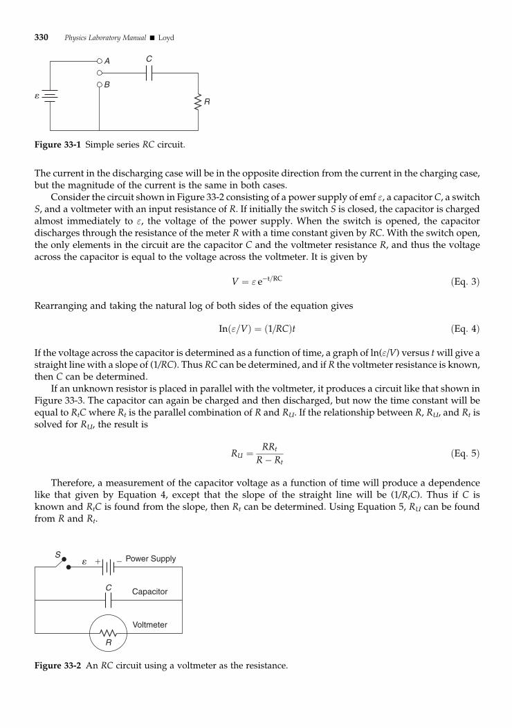
The current in the discharging case will be in the opposite direction from the current in the charging case,but the magnitude of the current is the same in both cases.
Consider the circuit shown in Figure 33-2 consisting of a power supply of emf ", a capacitor C, a switchS, and a voltmeter with an input resistance of R. If initially the switch S is closed, the capacitor is chargedalmost immediately to ", the voltage of the power supply. When the switch is opened, the capacitordischarges through the resistance of the meter Rwith a time constant given by RC. With the switch open,the only elements in the circuit are the capacitor C and the voltmeter resistance R, and thus the voltageacross the capacitor is equal to the voltage across the voltmeter. It is given by
V ¼ " e�t=RC ðEq: 3Þ
Rearranging and taking the natural log of both sides of the equation gives
Inð"=VÞ ¼ ð1=RCÞt ðEq: 4Þ
If the voltage across the capacitor is determined as a function of time, a graph of ln("/V) versus twill give astraight line with a slope of (1/RC). Thus RC can be determined, and if R the voltmeter resistance is known,then C can be determined.
If an unknown resistor is placed in parallel with the voltmeter, it produces a circuit like that shown inFigure 33-3. The capacitor can again be charged and then discharged, but now the time constant will beequal to RtCwhere Rt is the parallel combination of R and RU. If the relationship between R, RU, and Rt issolved for RU, the result is
RU ¼ RRt
R� RtðEq: 5Þ
Therefore, a measurement of the capacitor voltage as a function of time will produce a dependencelike that given by Equation 4, except that the slope of the straight line will be (1/RtC). Thus if C isknown and RtC is found from the slope, then Rt can be determined. Using Equation 5, RU can be foundfrom R and Rt.
� � �S Power Supply
Capacitor
Voltmeter
C
R
Figure 33-2 An RC circuit using a voltmeter as the resistance.
�
CA
B
R
Figure 33-1 Simple series RC circuit.
330 Physics Laboratory Manual n Loyd
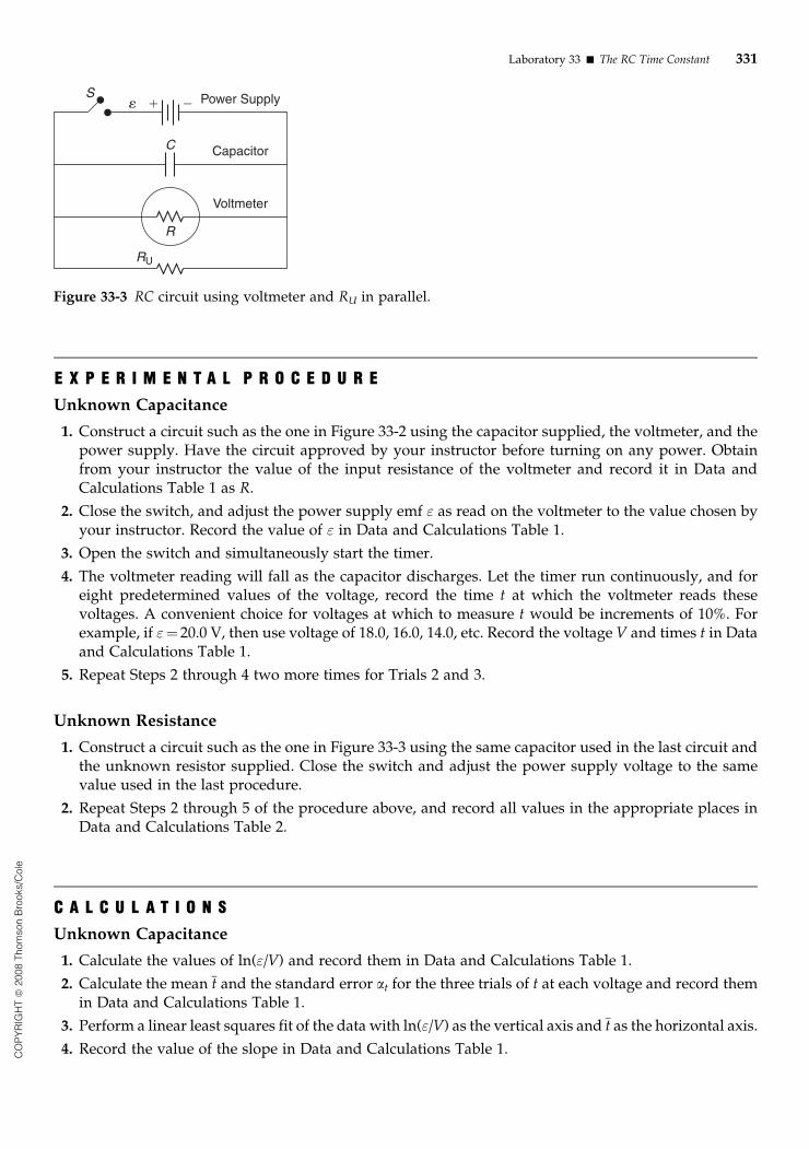
E X P E R I M E N T A L P R O C E D U R EUnknown Capacitance
1. Construct a circuit such as the one in Figure 33-2 using the capacitor supplied, the voltmeter, and thepower supply. Have the circuit approved by your instructor before turning on any power. Obtainfrom your instructor the value of the input resistance of the voltmeter and record it in Data andCalculations Table 1 as R.
2. Close the switch, and adjust the power supply emf " as read on the voltmeter to the value chosen byyour instructor. Record the value of " in Data and Calculations Table 1.
3. Open the switch and simultaneously start the timer.
4. The voltmeter reading will fall as the capacitor discharges. Let the timer run continuously, and foreight predetermined values of the voltage, record the time t at which the voltmeter reads thesevoltages. A convenient choice for voltages at which to measure t would be increments of 10%. Forexample, if "¼ 20.0 V, then use voltage of 18.0, 16.0, 14.0, etc. Record the voltage V and times t in Dataand Calculations Table 1.
5. Repeat Steps 2 through 4 two more times for Trials 2 and 3.
Unknown Resistance
1. Construct a circuit such as the one in Figure 33-3 using the same capacitor used in the last circuit andthe unknown resistor supplied. Close the switch and adjust the power supply voltage to the samevalue used in the last procedure.
2. Repeat Steps 2 through 5 of the procedure above, and record all values in the appropriate places inData and Calculations Table 2.
C A L C U L A T I O N SUnknown Capacitance
1. Calculate the values of ln("/V) and record them in Data and Calculations Table 1.
2. Calculate the mean t and the standard error at for the three trials of t at each voltage and record themin Data and Calculations Table 1.
3. Perform a linear least squares fit of the data with ln("/V) as the vertical axis and t as the horizontal axis.
4. Record the value of the slope in Data and Calculations Table 1.COPYRIG
HTª
2008ThomsonBrooks/Cole
� � �S Power Supply
Capacitor
Voltmeter
C
R
RU
Figure 33-3 RC circuit using voltmeter and RU in parallel.
Laboratory 33 n The RC Time Constant 331
5. Calculate RC as the reciprocal of the slope. Record the value of RC in Data and Calculations Table 1.
6. Use the value of RC and the value of R to calculate the value of the unknown capacitor C and record itin Data and Calculations Table 1.
Unknown Resistance
1. Calculate the values of ln("/V) and record the values in Data and Calculations Table 2.
2. Calculate the mean t and the standard error at for the three trials of t at each voltage and record themin Data and Calculations Table 2.
3. Perform a linear least squares fit of the data with ln("/V) as the vertical axis and t as the horizontal axis.
4. Record the value of the slope in Data and Calculations Table 2.
5. Calculate the value of RtC as the reciprocal of the slope. Record the value of RtC in Data andCalculations Table 2.
6. Using the value of the capacitance C determined in the first procedure and the value of RtC, calculatethe value of Rt and record it in Data and Calculations Table 2.
7. Calculate the value of the unknown resistance RU from the values of Rt and R. Record the value of RU
in Data and Calculations Table 2.
G R A P H S1. For the data from Data and Calculations Table 1 graph the quantity ln("/V) as the vertical axis and t as
the horizontal axis. Also show on the graph the straight line obtained from the linear least squares fitto the data.
2. For the data fromData and Calculations Table 2, graph the quantity ln("/V) as the vertical axis and t asthe horizontal axis. Also show on the graph the straight line obtained from the linear least squares fitto the data.
332 Physics Laboratory Manual n Loyd

Name . . . . . . . . . . . . . . . . . . . . . . . . . . . . . . . . . . . . . . . . . . . . . . . . . . . . . . . . . . . . . . . . . . . . . . . . . Section . . . . . . . . . . . . . . . . Date . . . . . . . . . . . . . . . .
33 L A B O R A T O R Y 3 3 The RC Time Constant
P R E - L A B O R A T O R Y A S S I G N M E N T1. In a circuit such as the one in Figure 33-1 with the capacitor initially uncharged, the switch S is thrown
to position A at t¼ 0. The charge on the capacitor (a) is initially zero and finally C" (b) is constant at avalue of C" (c) is initially C" and finally zero (d) is always less than "/R.
2. In a circuit such as the one in Figure 33-1 with the capacitor initially uncharged, the switch S is thrownto position A at t¼ 0. The current in the circuit is (a) initially zero and finally "/R (b) constant at a valueof "/R (c) equal to C" (d) initially "/R and finally zero.
3. In a circuit such as the one in Figure 33-2 the switch S is first closed to charge the capacitor, and then itis opened at t¼ 0. The expression V¼ " e�t/RC gives the value of (a) the voltage on the capacitor butnot the voltmeter (b) the voltage on the voltmeter but not the capacitor (c) both the voltage on thecapacitor and the voltage on the voltmeter, which are the same (d) the charge on the capacitor.
4. For a circuit such as the one in Figure 33-1, what are the equations for the charge Q and the current Ias functions of time when the capacitor is charging?
Q ¼ I ¼
5. For a circuit such as the one in Figure 33-1, what are the equations for the charge Q and the current Ias functions of time when the capacitor is discharging?
Q ¼ I ¼
6. If a 5.00 mF capacitor and a 3.50 MO resistor form a series RC circuit, what is the RC time constant?Give proper units for RC and show your work.
RC ¼
COPYRIG
HTª
2008ThomsonBrooks/Cole
333
7. Assume that a 10.0 mF capacitor, a battery of emf "¼ 12.0V, and a voltmeter of 10.0 MO inputimpedance are used in a circuit such as that in Figure 33-2. The switch S is first closed, and then theswitch is opened. What is the reading on the voltmeter 35.0 s after the switch is opened? Show yourwork.
V ¼ V
8. Assume that a circuit is constructed such as the one shown in Figure 33-3 with a capacitor of 5.00 mF, abattery of 24.0 V, a voltmeter of input impedance 12.0 MO, and a resistor RU¼ 10.0 MO. If the switch isfirst closed and then opened, what is the voltmeter reading 25.0 s after the switch is opened? Showyour work.
V ¼ V
9. In the measurement of the voltage as a function of time performed in this laboratory, the voltage ismeasured at fixed time intervals. (a) true (b) false
334 Physics Laboratory Manual n Loyd

Name . . . . . . . . . . . . . . . . . . . . . . . . . . . . . . . . . . . . . . . . . . . . . . . . . . . . . . . . . . . . . . . . . . . . . . . . . Section . . . . . . . . . . . . . . . . Date . . . . . . . . . . . . . . . .
Lab Partners . . . . . . . . . . . . . . . . . . . . . . . . . . . . . . . . . . . . . . . . . . . . . . . . . . . . . . . . . . . . . . . . . . . . . . . . . . . . . . . . . . . . . . . . . . . . . . . . . . . . . . . . . . . . . . . . . . . .
33 L A B O R A T O R Y 3 3 The RC Time Constant
L A B O R A T O R Y R E P O R T
COPYRIG
HTª
2008ThomsonBrooks/Cole
Data and Calculations Table 1
V (V) t1 (s) t2 (s) t3 (s) ln("/V) t (s) at (s)
"¼ V R¼ O r¼ Intercept¼
Slope¼ s�1 RC¼ s C¼ F
335
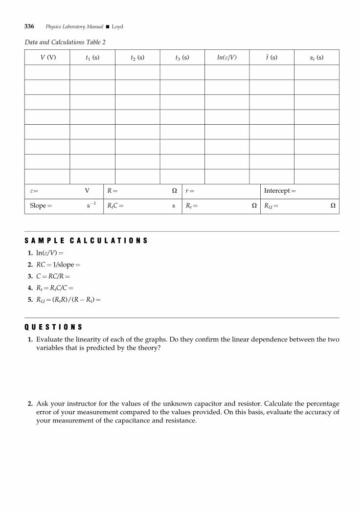
S A M P L E C A L C U L A T I O N S1. ln("/V)¼2. RC¼ 1/slope¼3. C¼RC/R¼4. Rt¼RtC/C¼5. RU¼ (RtR)/(R�Rt)¼
Q U E S T I O N S1. Evaluate the linearity of each of the graphs. Do they confirm the linear dependence between the two
variables that is predicted by the theory?
2. Ask your instructor for the values of the unknown capacitor and resistor. Calculate the percentageerror of your measurement compared to the values provided. On this basis, evaluate the accuracy ofyour measurement of the capacitance and resistance.
Data and Calculations Table 2
V (V) t1 (s) t2 (s) t3 (s) ln("/V) t (s) at (s)
"¼ V R¼ O r¼ Intercept¼
Slope¼ s�1 RtC¼ s Rt¼ O RU¼ O
336 Physics Laboratory Manual n Loyd

3. Show that RC has units of seconds if R is in O and C is in F.
4. A capacitor of 5.60 mF and a 4.57 MO resistor form a series RC circuit. If the capacitor is initiallycharged to 25.0 V, how long does it take for the voltage on the capacitor to reach 10.0 V? Show yourwork.
COPYRIG
HTª
2008ThomsonBrooks/Cole
Laboratory 33 n The RC Time Constant 337

This page intentionally left blank

Kirchhoff’s Rules
O B J E C T I V E So Investigate what type of circuit to which Kirchhoff’s rules must be applied.
o Apply Kirchhoff’s rules to several circuits, solve for the currents in the circuit, and compare thetheoretical values predicted by Kirchhoff’s rules to measured values.
E Q U I P M E N T L I S T. Direct current voltmeter (digital, 0–20 V), direct current ammeter (digital, 0–1000 mA)
. Two sources of emf (direct current power supplies, up to 12 V)
. Three or four resistors or resistor boxes (range 500–1000O)
. Digital ohmmeter (one for the class), connecting wires
T H E O R YConsider the circuit in Figure 34-1. The circuit is labeled with all of the currents. The 2O resistor, 8Oresistor, and 12V power supply have current I1, the 6O resistor has current I2, and the 3O resistor hascurrent I3. This circuit is called a single-loop circuit because it can be reduced to a single resistor in serieswith the power supply. The 6O resistor and the 3O resistor are in parallel with an equivalent resistanceof 2O. That equivalent 2O resistance is in series with the 12V power supply and the other two resistors,reducing the circuit to a single-loop circuit. The total resistance across the 12V power supply is 12O andits current is therefore I1¼ 1A. Applying Ohm’s law to the remaining part of the circuit gives I2¼ 1/3Aand I3¼ 2/3A.
Consider now the circuit of Figure 34-2. This laboratory is concerned with the fundamental differencebetween circuits of the type depicted in Figure 34-1 and circuits of the type depicted in Figure 34-2. Thecircuit in Figure 34-2 cannot be reduced to a single-loop circuit, but instead is called a multi-loop circuit.Before analyzing this circuit, first we will define some terms. A point at which at least three possiblecurrent paths intersect is defined as a junction. For example, points A and B in Figure 34-2 are junctions.A closed loop is any path that starts at some point in a circuit and passes through elements of the circuit (inthis case resistors and power supplies), and then arrives back at the same point without passing throughany circuit element more than once. By this definition there are three loops in the circuit of Figure 34-2:(1) starting at B, going through the 10V power supply toA, and then down through the 20V power supplyback toB, (2) starting atB, up through the 20V power supply, and then around the outside through the 10Oresistor and back toB, (3) completely around the outside part of the circuit. One can traverse a loop in eitherof two directions, but regardless of which direction is chosen, the resulting equations are equivalent.
Physics Laboratory Manual n Loyd L A B O R A T O R Y 34
COPYRIG
HTª
2008ThomsonBrooks/Cole
339
ª 2008 Thomson Brooks/Cole, a part of TheThomson Corporation.Thomson, the Star logo, and Brooks/Cole are trademarks used herein under license. ALL RIGHTSRESERVED.No part of this workcovered by the copyright hereonmay be reproduced or used in any form or by any meansçgraphic, electronic, ormechanical, including photocopying, recording, taping,web distribution, informationstorage and retrieval systems,or in any othermannerçwithout the written permission of the publisher.
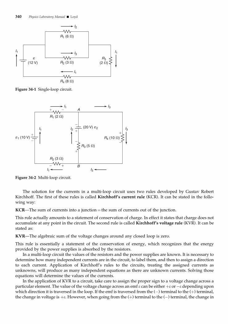
The solution for the currents in a multi-loop circuit uses two rules developed by Gustav RobertKirchhoff. The first of these rules is called Kirchhoff’s current rule (KCR). It can be stated in the follo-wing way:
KCR—The sum of currents into a junction¼ the sum of currents out of the junction.
This rule actually amounts to a statement of conservation of charge. In effect it states that charge does notaccumulate at any point in the circuit. The second rule is called Kirchhoff’s voltage rule (KVR). It can bestated as:
KVR—The algebraic sum of the voltage changes around any closed loop is zero.
This rule is essentially a statement of the conservation of energy, which recognizes that the energyprovided by the power supplies is absorbed by the resistors.
In a multi-loop circuit the values of the resistors and the power supplies are known. It is necessary todetermine how many independent currents are in the circuit, to label them, and then to assign a directionto each current. Application of Kirchhoff’s rules to the circuits, treating the assigned currents asunknowns, will produce as many independent equations as there are unknown currents. Solving thoseequations will determine the values of the currents.
In the application of KVR to a circuit, take care to assign the proper sign to a voltage change across aparticular element. The value of the voltage change across an emf e can be eitherþe or�e depending uponwhich direction it is traversed in the loop. If the emf is traversed from the (�) terminal to the (þ) terminal,the change in voltage isþe. However, when going from the (þ) terminal to the (�) terminal, the change in
�(12 V)
I2
I3
I1
R3(2 �)
R1 (6 �)
R2 (3 �)
R4 (8 �)
I1I1
Figure 34-1 Single-loop circuit.
I1 I3A
B
R1 (2 �)
R4 (10 �)
(20 V) �2
R3 (5 �)
I1 I3
R2 (3 �)
I3
�1 (10 V)
I1 I2�
��
�
�
�
�
�
� �
� �
Figure 34-2 Multi-loop circuit.
340 Physics Laboratory Manual n Loyd
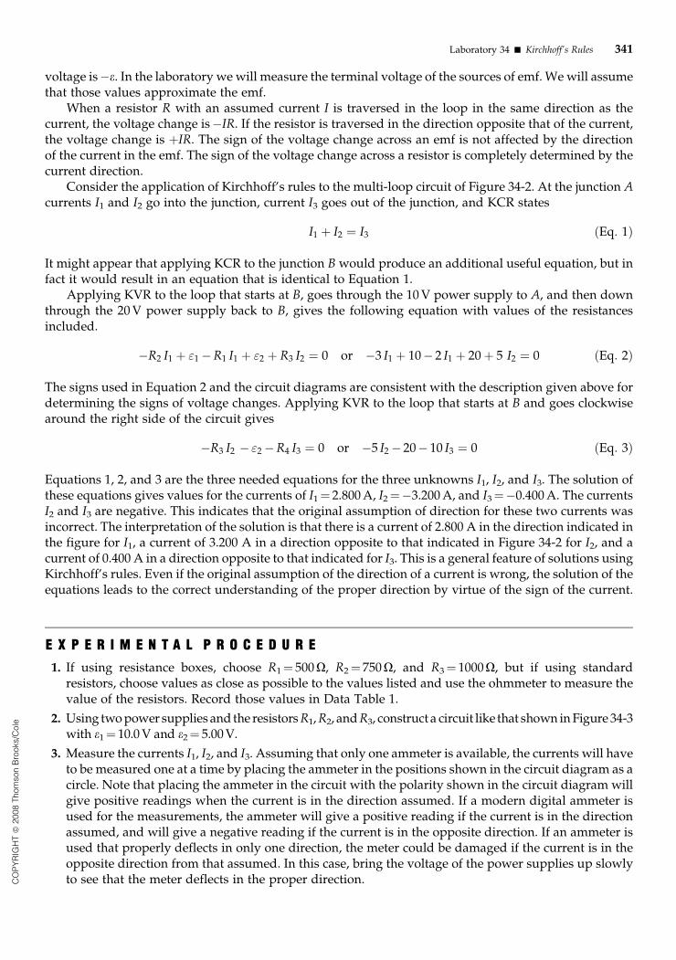
voltage is�e. In the laboratory we will measure the terminal voltage of the sources of emf. Wewill assumethat those values approximate the emf.
When a resistor R with an assumed current I is traversed in the loop in the same direction as thecurrent, the voltage change is�IR. If the resistor is traversed in the direction opposite that of the current,the voltage change is þIR. The sign of the voltage change across an emf is not affected by the directionof the current in the emf. The sign of the voltage change across a resistor is completely determined by thecurrent direction.
Consider the application of Kirchhoff’s rules to the multi-loop circuit of Figure 34-2. At the junction Acurrents I1 and I2 go into the junction, current I3 goes out of the junction, and KCR states
I1 þ I2 ¼ I3 ðEq: 1Þ
It might appear that applying KCR to the junction Bwould produce an additional useful equation, but infact it would result in an equation that is identical to Equation 1.
Applying KVR to the loop that starts at B, goes through the 10V power supply to A, and then downthrough the 20V power supply back to B, gives the following equation with values of the resistancesincluded.
�R2 I1 þ "1 �R1 I1 þ "2 þ R3 I2 ¼ 0 or �3 I1 þ 10� 2 I1 þ 20þ 5 I2 ¼ 0 ðEq: 2Þ
The signs used in Equation 2 and the circuit diagrams are consistent with the description given above fordetermining the signs of voltage changes. Applying KVR to the loop that starts at B and goes clockwisearound the right side of the circuit gives
�R3 I2 � "2 �R4 I3 ¼ 0 or �5 I2 � 20� 10 I3 ¼ 0 ðEq: 3Þ
Equations 1, 2, and 3 are the three needed equations for the three unknowns I1, I2, and I3. The solution ofthese equations gives values for the currents of I1¼ 2.800A, I2¼�3.200A, and I3¼�0.400A. The currentsI2 and I3 are negative. This indicates that the original assumption of direction for these two currents wasincorrect. The interpretation of the solution is that there is a current of 2.800 A in the direction indicated inthe figure for I1, a current of 3.200 A in a direction opposite to that indicated in Figure 34-2 for I2, and acurrent of 0.400 A in a direction opposite to that indicated for I3. This is a general feature of solutions usingKirchhoff’s rules. Even if the original assumption of the direction of a current is wrong, the solution of theequations leads to the correct understanding of the proper direction by virtue of the sign of the current.
E X P E R I M E N T A L P R O C E D U R E1. If using resistance boxes, choose R1¼ 500O, R2¼ 750O, and R3¼ 1000O, but if using standard
resistors, choose values as close as possible to the values listed and use the ohmmeter to measure thevalue of the resistors. Record those values in Data Table 1.
2. Using twopower supplies and the resistorsR1,R2, andR3, construct a circuit like that shown inFigure 34-3with e1¼ 10.0V and e2¼ 5.00V.
3. Measure the currents I1, I2, and I3. Assuming that only one ammeter is available, the currents will haveto be measured one at a time by placing the ammeter in the positions shown in the circuit diagram as acircle. Note that placing the ammeter in the circuit with the polarity shown in the circuit diagram willgive positive readings when the current is in the direction assumed. If a modern digital ammeter isused for the measurements, the ammeter will give a positive reading if the current is in the directionassumed, and will give a negative reading if the current is in the opposite direction. If an ammeter isused that properly deflects in only one direction, the meter could be damaged if the current is in theopposite direction from that assumed. In this case, bring the voltage of the power supplies up slowlyto see that the meter deflects in the proper direction.C
OPYRIG
HTª
2008ThomsonBrooks/Cole
Laboratory 34 n Kirchhoff’s Rules 341
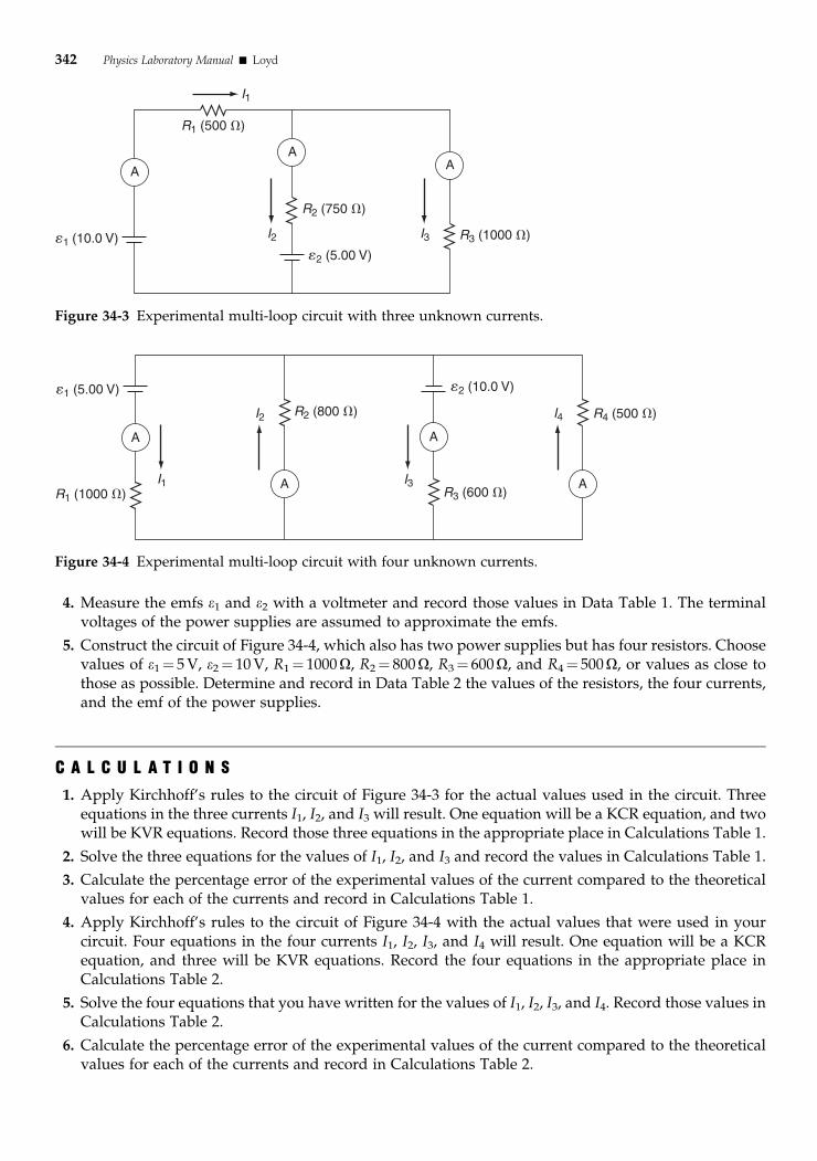
4. Measure the emfs e1 and e2 with a voltmeter and record those values in Data Table 1. The terminalvoltages of the power supplies are assumed to approximate the emfs.
5. Construct the circuit of Figure 34-4, which also has two power supplies but has four resistors. Choosevalues of e1¼ 5V, e2¼ 10V, R1¼ 1000O, R2¼ 800O, R3¼ 600O, and R4¼ 500O, or values as close tothose as possible. Determine and record in Data Table 2 the values of the resistors, the four currents,and the emf of the power supplies.
C A L C U L A T I O N S1. Apply Kirchhoff’s rules to the circuit of Figure 34-3 for the actual values used in the circuit. Three
equations in the three currents I1, I2, and I3 will result. One equation will be a KCR equation, and twowill be KVR equations. Record those three equations in the appropriate place in Calculations Table 1.
2. Solve the three equations for the values of I1, I2, and I3 and record the values in Calculations Table 1.
3. Calculate the percentage error of the experimental values of the current compared to the theoreticalvalues for each of the currents and record in Calculations Table 1.
4. Apply Kirchhoff’s rules to the circuit of Figure 34-4 with the actual values that were used in yourcircuit. Four equations in the four currents I1, I2, I3, and I4 will result. One equation will be a KCRequation, and three will be KVR equations. Record the four equations in the appropriate place inCalculations Table 2.
5. Solve the four equations that you have written for the values of I1, I2, I3, and I4. Record those values inCalculations Table 2.
6. Calculate the percentage error of the experimental values of the current compared to the theoreticalvalues for each of the currents and record in Calculations Table 2.
R1 (500 �)
R3 (1000 �)
R2 (750 �)
�2 (5.00 V)
I3�1 (10.0 V) I2
I1
A AA
Figure 34-3 Experimental multi-loop circuit with three unknown currents.
R4 (500 �)
�2 (10.0 V)
R3 (600 �)
I4
I3 A
A
�1 (5.00 V)
R1 (1000 �)I1
A
R2 (800 �)I2
A
Figure 34-4 Experimental multi-loop circuit with four unknown currents.
342 Physics Laboratory Manual n Loyd
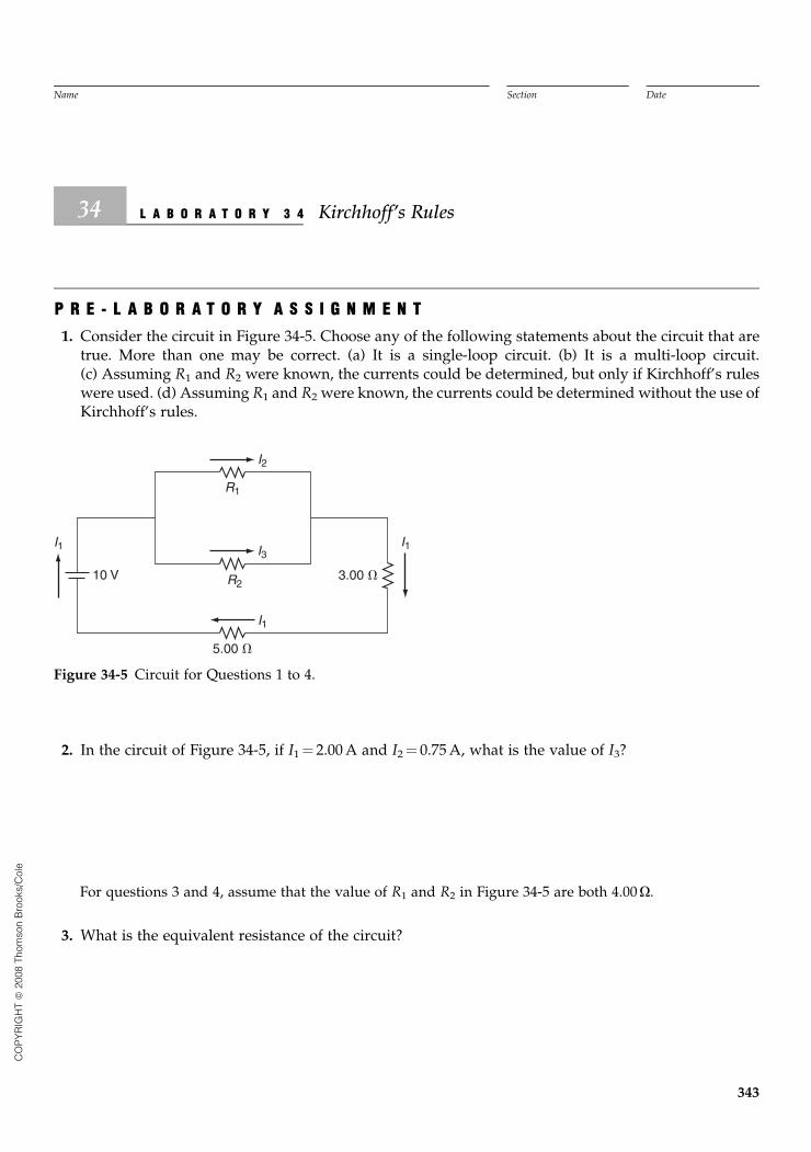
Name . . . . . . . . . . . . . . . . . . . . . . . . . . . . . . . . . . . . . . . . . . . . . . . . . . . . . . . . . . . . . . . . . . . . . . . . . Section . . . . . . . . . . . . . . . . Date . . . . . . . . . . . . . . . .
34 L A B O R A T O R Y 3 4 Kirchhoff’s Rules
P R E - L A B O R A T O R Y A S S I G N M E N T1. Consider the circuit in Figure 34-5. Choose any of the following statements about the circuit that are
true. More than one may be correct. (a) It is a single-loop circuit. (b) It is a multi-loop circuit.(c) Assuming R1 and R2 were known, the currents could be determined, but only if Kirchhoff’s ruleswere used. (d) Assuming R1 and R2 were known, the currents could be determined without the use ofKirchhoff’s rules.
2. In the circuit of Figure 34-5, if I1¼ 2.00A and I2¼ 0.75A, what is the value of I3?
For questions 3 and 4, assume that the value of R1 and R2 in Figure 34-5 are both 4.00O.
3. What is the equivalent resistance of the circuit?
COPYRIG
HTª
2008ThomsonBrooks/Cole
10 V 3.00 �
5.00 �
I1
I3
I2
I1 I1
R1
R2
Figure 34-5 Circuit for Questions 1 to 4.
343
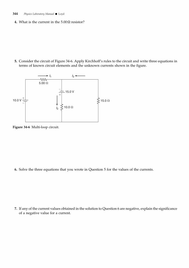
4. What is the current in the 5.00O resistor?
5. Consider the circuit of Figure 34-6. Apply Kirchhoff’s rules to the circuit and write three equations interms of known circuit elements and the unknown currents shown in the figure.
6. Solve the three equations that you wrote in Question 5 for the values of the currents.
7. If any of the current values obtained in the solution to Question 6 are negative, explain the significanceof a negative value for a current.
I1 I3
5.00 �
�
�
�
�
15.0 �
15.0 V
10.0 �
10.0 V
I2
Figure 34-6 Multi-loop circuit.
344 Physics Laboratory Manual n Loyd
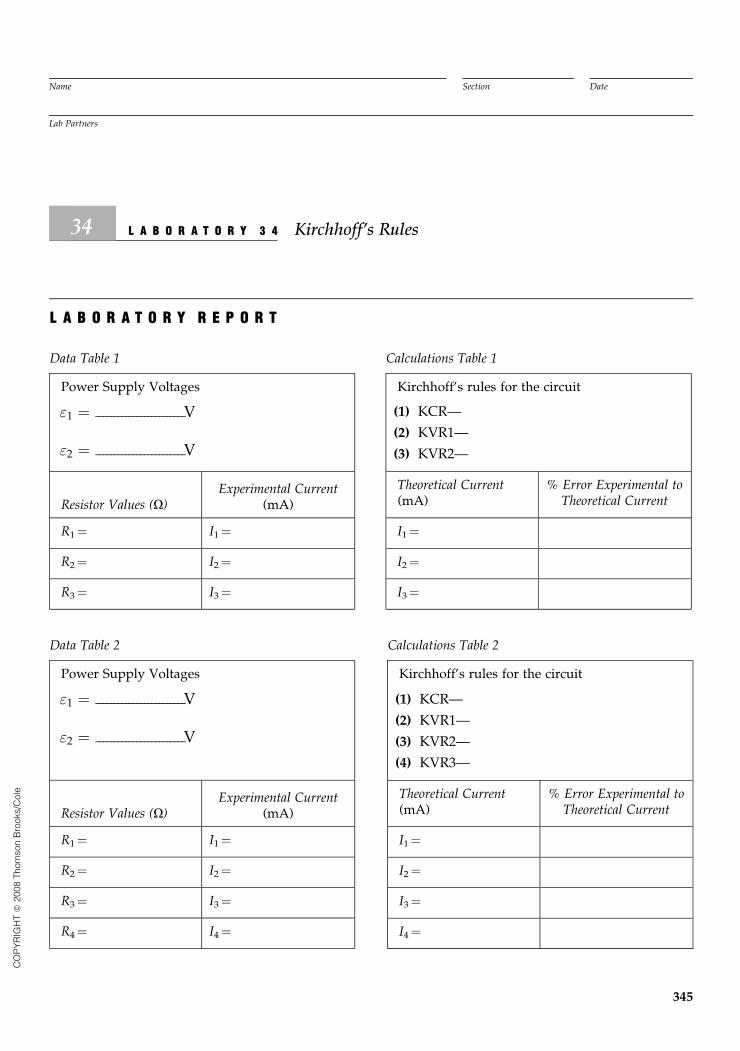
Name . . . . . . . . . . . . . . . . . . . . . . . . . . . . . . . . . . . . . . . . . . . . . . . . . . . . . . . . . . . . . . . . . . . . . . . . . Section . . . . . . . . . . . . . . . . Date . . . . . . . . . . . . . . . .
Lab Partners . . . . . . . . . . . . . . . . . . . . . . . . . . . . . . . . . . . . . . . . . . . . . . . . . . . . . . . . . . . . . . . . . . . . . . . . . . . . . . . . . . . . . . . . . . . . . . . . . . . . . . . . . . . . . . . . . . . .
34 L A B O R A T O R Y 3 4 Kirchhoff’s Rules
L A B O R A T O R Y R E P O R T
COPYRIG
HTª
2008ThomsonBrooks/Cole
Data Table 1
Power Supply Voltages
"1 ¼ V
"2 ¼ V
Resistor Values (O)Experimental Current
(mA)
R1¼ I1¼
R2¼ I2¼
R3¼ I3¼
Calculations Table 1
Kirchhoff’s rules for the circuit
(1) KCR—
(2) KVR1—
(3) KVR2—
Theoretical Current(mA)
% Error Experimental toTheoretical Current
I1¼
I2¼
I3¼
Data Table 2
Power Supply Voltages
"1 ¼ V
"2 ¼ V
Resistor Values (O)Experimental Current
(mA)
R1¼ I1¼
R2¼ I2¼
R3¼ I3¼
R4¼ I4¼
Calculations Table 2
Kirchhoff’s rules for the circuit
(1) KCR—
(2) KVR1—
(3) KVR2—
(4) KVR3—
Theoretical Current(mA)
% Error Experimental toTheoretical Current
I1¼
I2¼
I3¼
I4¼
345
S A M P L E C A L C U L A T I O N S1. KCR, KVR1, and KVR2 provide three equations to be solved for I1, I2, and I3 for first circuit.
2. KCR, KVR1, KVR2, and KVR3 provide four equations to be solved for I1, I2, I3, and I4 for secondcircuit.
Q U E S T I O N S1. In Figure 34-3, state the equation that relates the currents I1, I2, and I3. Calculate the percentage
difference between the experimental values of the two sides of the equation.
2. In Figure 34-4, state the equation that relates the currents I1, I2, I3, and I4. Calculate the percentagedifference between the experimental values of the two sides of the equation.
3. Are the experimental values of the currents for the entire laboratory generally larger or smaller thanthe theoretical values expected for the currents?
346 Physics Laboratory Manual n Loyd

4. An ideal ammeter has zero resistance. Real ammeters have small but finite resistance.Would ammeterresistance cause an error in the proper direction to account for the direction of your error indicated inQuestion 3? State your reasoning.
5. The connecting wires in the experiment are assumed to have no resistance, but in fact have a finiteresistance. Would this error be in the proper direction to account for the direction of the error stated inyour answer to Question 3? State your reasoning.
COPYRIG
HTª
2008ThomsonBrooks/Cole
Laboratory 34 n Kirchhoff’s Rules 347

This page intentionally left blank

Magnetic Inductionof a Current CarryingLong Straight Wire
O B J E C T I V E So Use a compass to determine the direction of the B field surrounding a current carrying long
straight wire to confirm that it is consistent with the right-hand rule.
o Determine the induced voltage in a small inductor coil placed near the long straight wire as arelative measurement of the B field.
o Demonstrate that the magnitude of the B field surrounding a long straight wire decreases as 1/rwhere r is the perpendicular distance from the wire.
E Q U I P M E N T L I S T. Direct current power supply (low voltage, 2 A), direct current ammeter (2A)
. Sine wave generator (variable frequency up to 100 kHz, 5 V peak to peak)
. Alternating current digital voltmeter (frequencies up to 100 kHz)
. 100-mH inductor coil (length� 1 cm and inside diameter� 1 cm)
. Small compass, long straight wire apparatus (Consists of a frame on which a continuous strand of wireis wrapped for 10 loops. The 10 strands are taped together over a length of approximately 40 cm toapproximate a wire with a current having 10 times the current as in a single strand of the wire. Theapparatus can be placedwith the long straight section parallel to the laboratory table or perpendicular tothe table.)
T H E O R YWhen a current I exists in an infinitely long straight wire, the lines of magnetic induction B are con-centric circles surrounding the wire. At a perpendicular distance r from the wire, the B field is tangent tothe circle as shown in Figure 35-1. The direction of the current I is perpendicular to the plane of thepage and directed out of the page. The direction of the current is by definition the direction that positivecharge would flow. The magnitude of the B field as a function of I and r is given by
Physics Laboratory Manual n Loyd L A B O R A T O R Y 35
COPYRIG
HTª
2008ThomsonBrooks/Cole
349
ª 2008 Thomson Brooks/Cole, a part of TheThomson Corporation.Thomson, the Star logo, and Brooks/Cole are trademarks used herein under license. ALL RIGHTSRESERVED.No part of this workcovered by the copyright hereonmay be reproduced or used in any form or by any meansçgraphic, electronic, ormechanical, including photocopying, recording, taping,web distribution, informationstorage and retrieval systems,or in any othermannerçwithout the written permission of the publisher.
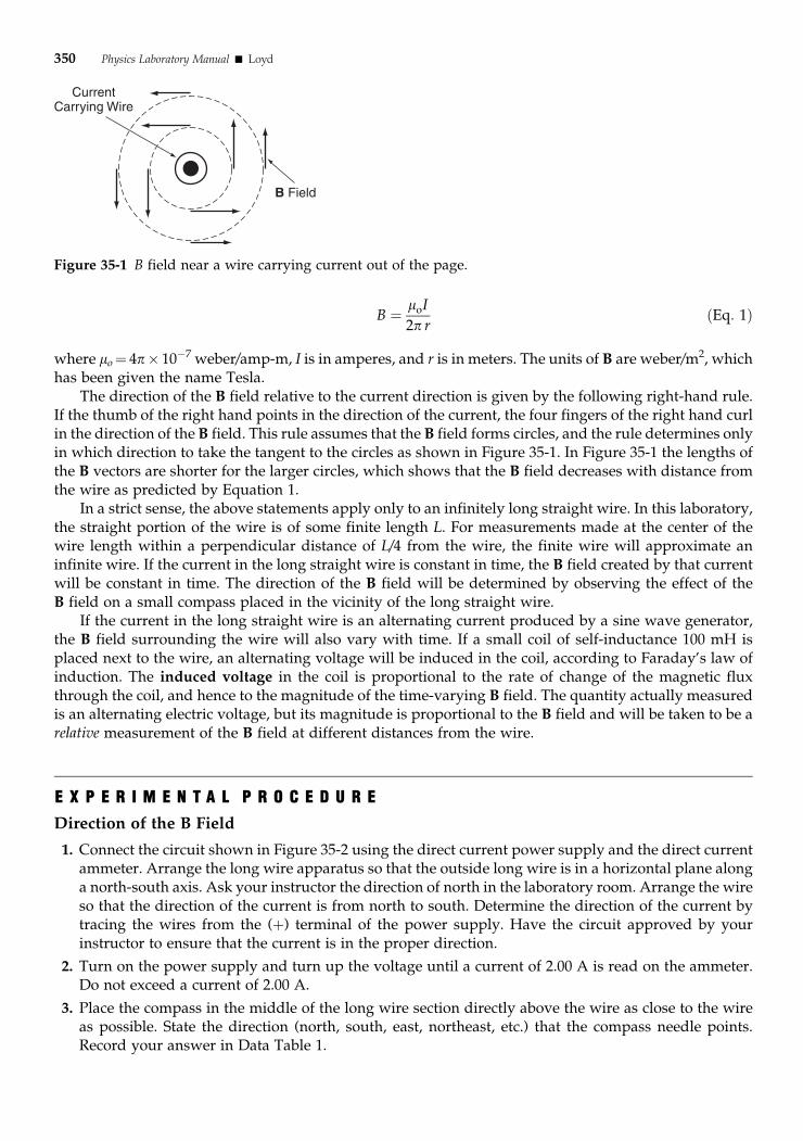
B ¼ moI2p r
ðEq: 1Þ
where mo¼ 4p� 10�7 weber/amp-m, I is in amperes, and r is in meters. The units of B are weber/m2, whichhas been given the name Tesla.
The direction of the B field relative to the current direction is given by the following right-hand rule.If the thumb of the right hand points in the direction of the current, the four fingers of the right hand curlin the direction of the B field. This rule assumes that the B field forms circles, and the rule determines onlyin which direction to take the tangent to the circles as shown in Figure 35-1. In Figure 35-1 the lengths ofthe B vectors are shorter for the larger circles, which shows that the B field decreases with distance fromthe wire as predicted by Equation 1.
In a strict sense, the above statements apply only to an infinitely long straight wire. In this laboratory,the straight portion of the wire is of some finite length L. For measurements made at the center of thewire length within a perpendicular distance of L/4 from the wire, the finite wire will approximate aninfinite wire. If the current in the long straight wire is constant in time, the B field created by that currentwill be constant in time. The direction of the B field will be determined by observing the effect of theB field on a small compass placed in the vicinity of the long straight wire.
If the current in the long straight wire is an alternating current produced by a sine wave generator,the B field surrounding the wire will also vary with time. If a small coil of self-inductance 100 mH isplaced next to the wire, an alternating voltage will be induced in the coil, according to Faraday’s law ofinduction. The induced voltage in the coil is proportional to the rate of change of the magnetic fluxthrough the coil, and hence to the magnitude of the time-varying B field. The quantity actually measuredis an alternating electric voltage, but its magnitude is proportional to the B field and will be taken to be arelative measurement of the B field at different distances from the wire.
E X P E R I M E N T A L P R O C E D U R EDirection of the B Field
1. Connect the circuit shown in Figure 35-2 using the direct current power supply and the direct currentammeter. Arrange the long wire apparatus so that the outside long wire is in a horizontal plane alonga north-south axis. Ask your instructor the direction of north in the laboratory room. Arrange the wireso that the direction of the current is from north to south. Determine the direction of the current bytracing the wires from the (þ) terminal of the power supply. Have the circuit approved by yourinstructor to ensure that the current is in the proper direction.
2. Turn on the power supply and turn up the voltage until a current of 2.00 A is read on the ammeter.Do not exceed a current of 2.00 A.
3. Place the compass in the middle of the long wire section directly above the wire as close to the wireas possible. State the direction (north, south, east, northeast, etc.) that the compass needle points.Record your answer in Data Table 1.
B Field
CurrentCarrying Wire
Figure 35-1 B field near a wire carrying current out of the page.
350 Physics Laboratory Manual n Loyd
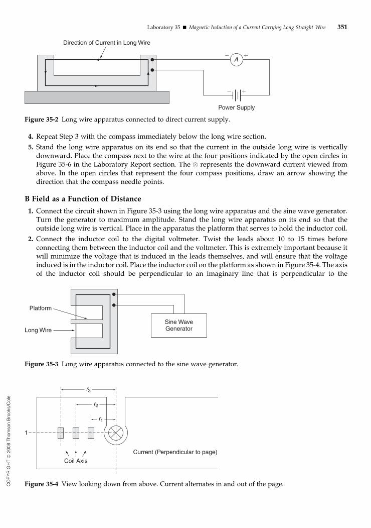
4. Repeat Step 3 with the compass immediately below the long wire section.
5. Stand the long wire apparatus on its end so that the current in the outside long wire is verticallydownward. Place the compass next to the wire at the four positions indicated by the open circles inFigure 35-6 in the Laboratory Report section. The represents the downward current viewed fromabove. In the open circles that represent the four compass positions, draw an arrow showing thedirection that the compass needle points.
B Field as a Function of Distance
1. Connect the circuit shown in Figure 35-3 using the long wire apparatus and the sine wave generator.Turn the generator to maximum amplitude. Stand the long wire apparatus on its end so that theoutside long wire is vertical. Place in the apparatus the platform that serves to hold the inductor coil.
2. Connect the inductor coil to the digital voltmeter. Twist the leads about 10 to 15 times beforeconnecting them between the inductor coil and the voltmeter. This is extremely important because itwill minimize the voltage that is induced in the leads themselves, and will ensure that the voltageinduced is in the inductor coil. Place the inductor coil on the platform as shown in Figure 35-4. The axisof the inductor coil should be perpendicular to an imaginary line that is perpendicular to the
COPYRIG
HTª
2008ThomsonBrooks/Cole
� �
� �
Power Supply
Direction of Current in Long Wire
A
Figure 35-2 Long wire apparatus connected to direct current supply.
Platform
Sine WaveGeneratorLong Wire
Figure 35-3 Long wire apparatus connected to the sine wave generator.
1
Current (Perpendicular to page)
Coil Axis
r3
r2
r1
Figure 35-4 View looking down from above. Current alternates in and out of the page.
Laboratory 35 n Magnetic Induction of a Current Carrying Long Straight Wire 351
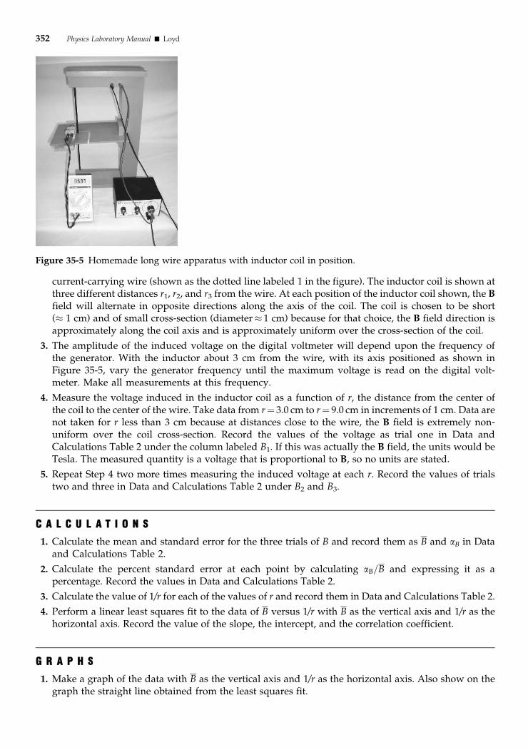
current-carrying wire (shown as the dotted line labeled 1 in the figure). The inductor coil is shown atthree different distances r1, r2, and r3 from the wire. At each position of the inductor coil shown, the Bfield will alternate in opposite directions along the axis of the coil. The coil is chosen to be short(� 1 cm) and of small cross-section (diameter� 1 cm) because for that choice, the B field direction isapproximately along the coil axis and is approximately uniform over the cross-section of the coil.
3. The amplitude of the induced voltage on the digital voltmeter will depend upon the frequency ofthe generator. With the inductor about 3 cm from the wire, with its axis positioned as shown inFigure 35-5, vary the generator frequency until the maximum voltage is read on the digital volt-meter. Make all measurements at this frequency.
4. Measure the voltage induced in the inductor coil as a function of r, the distance from the center ofthe coil to the center of the wire. Take data from r¼ 3.0 cm to r¼ 9.0 cm in increments of 1 cm. Data arenot taken for r less than 3 cm because at distances close to the wire, the B field is extremely non-uniform over the coil cross-section. Record the values of the voltage as trial one in Data andCalculations Table 2 under the column labeled B1. If this was actually the B field, the units would beTesla. The measured quantity is a voltage that is proportional to B, so no units are stated.
5. Repeat Step 4 two more times measuring the induced voltage at each r. Record the values of trialstwo and three in Data and Calculations Table 2 under B2 and B3.
C A L C U L A T I O N S1. Calculate the mean and standard error for the three trials of B and record them as B and aB in Data
and Calculations Table 2.
2. Calculate the percent standard error at each point by calculating aB=B and expressing it as apercentage. Record the values in Data and Calculations Table 2.
3. Calculate the value of 1/r for each of the values of r and record them in Data and Calculations Table 2.
4. Perform a linear least squares fit to the data of B versus 1/r with B as the vertical axis and 1/r as thehorizontal axis. Record the value of the slope, the intercept, and the correlation coefficient.
G R A P H S1. Make a graph of the data with B as the vertical axis and 1/r as the horizontal axis. Also show on the
graph the straight line obtained from the least squares fit.
Figure 35-5 Homemade long wire apparatus with inductor coil in position.
352 Physics Laboratory Manual n Loyd
Name . . . . . . . . . . . . . . . . . . . . . . . . . . . . . . . . . . . . . . . . . . . . . . . . . . . . . . . . . . . . . . . . . . . . . . . . . Section . . . . . . . . . . . . . . . . Date . . . . . . . . . . . . . . . .
35 L A B O R A T O R Y 3 5 Magnetic Induction of a Current CarryingLong Straight Wire
P R E - L A B O R A T O R Y A S S I G N M E N T1. State the right-hand rule that relates the direction of the B field near a long straight wire to the
direction of the current in the wire.
2. The direction of current is defined to be the direction in which _______________ charges would flow.
3. State the equation that relates the magnitude of the B field near a long straight wire to the current Iin the wire and the distance r from the wire.
B ¼
4. There is a current of 10.0 A in a long straight wire. What is the magnitude of the B field 5.00 cm fromthe wire? Show your work.
5. When a current that is constant in time passes through a wire, the B field that is produced around thewire is (a) time varying (b) constant in time (c) negative (d) zero.
COPYRIG
HTª
2008ThomsonBrooks/Cole
353

6. Why are measurements using the inductor coil not taken close to the wire? In other words, why do themeasurements start 3.00 cm away from the wire?
7. If an inductor coil is placed near a long wire carrying a current that is constant in time, the voltageinduced in the coil is (a) positive (b) negative (c) zero (d) nonzero.
354 Physics Laboratory Manual n Loyd
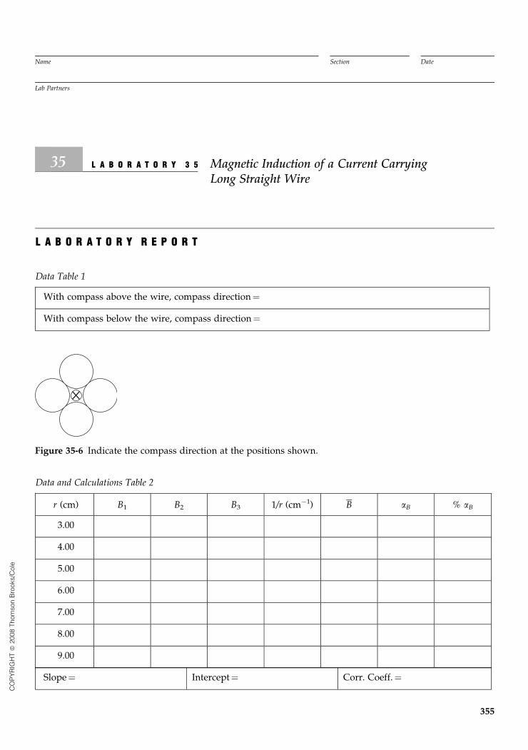
Name . . . . . . . . . . . . . . . . . . . . . . . . . . . . . . . . . . . . . . . . . . . . . . . . . . . . . . . . . . . . . . . . . . . . . . . . . Section . . . . . . . . . . . . . . . . Date . . . . . . . . . . . . . . . .
Lab Partners . . . . . . . . . . . . . . . . . . . . . . . . . . . . . . . . . . . . . . . . . . . . . . . . . . . . . . . . . . . . . . . . . . . . . . . . . . . . . . . . . . . . . . . . . . . . . . . . . . . . . . . . . . . . . . . . . . . .
35 L A B O R A T O R Y 3 5 Magnetic Induction of a Current CarryingLong Straight Wire
L A B O R A T O R Y R E P O R T
COPYRIG
HTª
2008ThomsonBrooks/Cole
Figure 35-6 Indicate the compass direction at the positions shown.
Data Table 1
With compass above the wire, compass direction¼
With compass below the wire, compass direction¼
Data and Calculations Table 2
r (cm) B1 B2 B3 1/r (cm�1) B aB % aB
3.00
4.00
5.00
6.00
7.00
8.00
9.00
Slope¼ Intercept¼ Corr. Coeff.¼
355
S A M P L E C A L C U L A T I O N S1. 1/r¼
Q U E S T I O N S1. Describe the reasoning used to apply the right-hand rule to the situations in Data Table 1, what is
predicted, and how your results do or do not agree with those predictions.
2. Evaluate the precision of the measurements of the induced voltage as a function of distance from thewire. Consider the percentage standard error of the measurements in your evaluation.
3. State the extent to which your measurements confirm the expectation that B is proportional to 1/r.Give the evidence for your evaluation of this question.
4. When the direct current is 2.00 A in a single wire of the bundle of 10 wires, the total current in thebundle of wire that approximates the long straight wire is 20.0 A. What is the magnitude of the B field3.00 cm from this long straight wire carrying a current of 20.0 A? What is the magnitude of theB field 9.00 cm from the wire carrying 20.0 A?
356 Physics Laboratory Manual n Loyd

5. A constant current is in a long straight wire in the plane of the paper in the direction shown belowby the arrow. Point X is in the plane of the paper above the wire, and point Y is in the plane of thepaper but below the wire. What is the direction of the B field at point X? What is the direction of theB field at point Y?
Y
X
Direction at X¼ ____________________________________________________________
Direction at Y¼ ____________________________________________________________
COPYRIG
HTª
2008ThomsonBrooks/Cole
Laboratory 35 n Magnetic Induction of a Current Carrying Long Straight Wire 357

This page intentionally left blank

Alternating CurrentLR Circuits
O B J E C T I V E So Investigate the phase angle of a generator current relative to the generator voltage.
o Demonstrate that real inductors consist of both inductance and resistance, and that they can berepresented by a pure inductor L in series with a pure resistance r.
o Determine the value of L and r for an unknown inductor.
E Q U I P M E N T L I S T. Sine wave generator (variable frequency, 5 V peak to peak amplitude), resistance box
. A 100-mH inductor (resistance� 350 O to serve as an unknown)
. Alternating current voltmeter (digital readout, high frequency capability), compass, protractor
T H E O R YConsider the two circuits shown in Figure 36-1 in which a sine wave generator of frequency f is connectedseparately to resistor R and then to a pure inductance L. The generator is assumed to have a maximumvoltage of V and will thus produce a maximum voltage of V across the resistor in circuit (a). It will alsoproduce a maximum voltage of V across the inductor in circuit (b). The voltage across the resistor isrelated to the current by a relationship like that for direct current circuits, which is
VR ¼ IR ðEq: 1Þ
If L is the inductance (units H) and o¼ 2pf is the angular frequency of the generator in rad/s, then thefollowing relationship exists between the voltage VL and the current I
VL ¼ IoL ðEq: 2Þ
The quantity oL is called the inductive reactance, and it has units of O.When an alternating current or voltage is measured in the laboratory on a meter, the number read for
the current or voltage must be a time-averaged value. Meters are normally calibrated so that they respondto the root-mean-square value of the current or voltage. A root-mean-square value of voltage is designated
Physics Laboratory Manual n Loyd L A B O R A T O R Y 36
COPYRIG
HTª
2008ThomsonBrooks/Cole
359
ª 2008 Thomson Brooks/Cole, a part of TheThomson Corporation.Thomson, the Star logo, and Brooks/Cole are trademarks used herein under license. ALL RIGHTSRESERVED.No part of this workcovered by the copyright hereonmay be reproduced or used in any form or by any meansçgraphic, electronic, ormechanical, including photocopying, recording, taping,web distribution, informationstorage and retrieval systems,or in any othermannerçwithout the written permission of the publisher.

asVrms. The relationship betweenVrms andV the maximum voltage isVrms¼ 0.707V. In this laboratory onlyvoltage will be measured, and all the measurements will be rms values.
Also shown in Figure 36-1 below each circuit is a graph of the current and voltage across the elementfor one full period. The graph for the case of the resistor indicates that the resistor current IR and theresistor voltage VR are in phase. For the inductor, the graph shows that the inductor current IL andthe inductor voltage VL are 908 out of phase, with the voltage leading the current by 908.
Shown at the bottom of Figure 36-1 is a diagram called a phasor diagram. Its purpose is also to show thephase relationship. The phasors are vectors drawn with length proportional to the value of the represen-ted quantity, and they are assumed to be rotating counterclockwise with the frequency of the generator.At any time, a projection of one of the rotating vectors on the y axis is the instantaneous value of thatquantity. Because the resistor current and voltage are in phase, the phasors are in the same direction. For theinductor, the vector representing the inductor voltage is 908 ahead of the vector representing the current.
Consider now the circuit obtained by placing a pure inductance L having no resistance and a resistorR in series with a sine wave generator of voltage V shown in Figure 36-2.
V R V L
IRVR
VL
IRVR
(a)
IL
VL
(b)
IL
Figure 36-1 Generator and resistor and generator and inductor. Phase relationships between the voltage andcurrent and phasor diagrams of the phase relationships.
V VL
VR
V
�R
L
Figure 36-2 Series circuit of resistor and inductor and associated phasor diagram.
360 Physics Laboratory Manual n Loyd
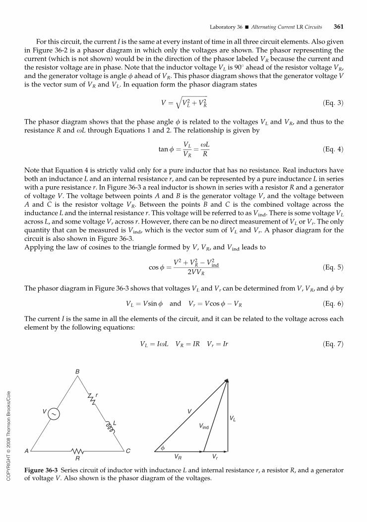
For this circuit, the current I is the same at every instant of time in all three circuit elements. Also givenin Figure 36-2 is a phasor diagram in which only the voltages are shown. The phasor representing thecurrent (which is not shown) would be in the direction of the phasor labeled VR because the current andthe resistor voltage are in phase. Note that the inductor voltage VL is 908 ahead of the resistor voltage VR,and the generator voltage is angle f ahead of VR. This phasor diagram shows that the generator voltage Vis the vector sum of VR and VL. In equation form the phasor diagram states
V ¼ffiffiffiffiffiffiffiffiffiffiffiffiffiffiffiffiffiffiV2
L þ V2R
qðEq: 3Þ
The phasor diagram shows that the phase angle f is related to the voltages VL and VR, and thus to theresistance R and oL through Equations 1 and 2. The relationship is given by
tanf ¼ VL
VR¼ oL
RðEq: 4Þ
Note that Equation 4 is strictly valid only for a pure inductor that has no resistance. Real inductors haveboth an inductance L and an internal resistance r, and can be represented by a pure inductance L in serieswith a pure resistance r. In Figure 36-3 a real inductor is shown in series with a resistor R and a generatorof voltage V. The voltage between points A and B is the generator voltage V, and the voltage betweenA and C is the resistor voltage VR. Between the points B and C is the combined voltage across theinductance L and the internal resistance r. This voltage will be referred to asVind. There is some voltageVL
across L, and some voltage Vr across r. However, there can be no direct measurement of VL or Vr. The onlyquantity that can be measured is Vind, which is the vector sum of VL and Vr. A phasor diagram for thecircuit is also shown in Figure 36-3.Applying the law of cosines to the triangle formed by V, VR, and Vind leads to
cosf ¼ V2 þ V2R � V2
ind
2VVRðEq: 5Þ
The phasor diagram in Figure 36-3 shows that voltages VL and Vr can be determined from V, VR, and f by
VL ¼ Vsinf and Vr ¼ Vcosf� VR ðEq: 6Þ
The current I is the same in all the elements of the circuit, and it can be related to the voltage across eachelement by the following equations:
VL ¼ IoL VR ¼ IR Vr ¼ Ir ðEq: 7Þ
COPYRIG
HTª
2008ThomsonBrooks/Cole
V
Vind
VL
VR VrA
R
L
r
C
B
�
V
Figure 36-3 Series circuit of inductor with inductance L and internal resistance r, a resistor R, and a generatorof voltage V. Also shown is the phasor diagram of the voltages.
Laboratory 36 n Alternating Current LR Circuits 361
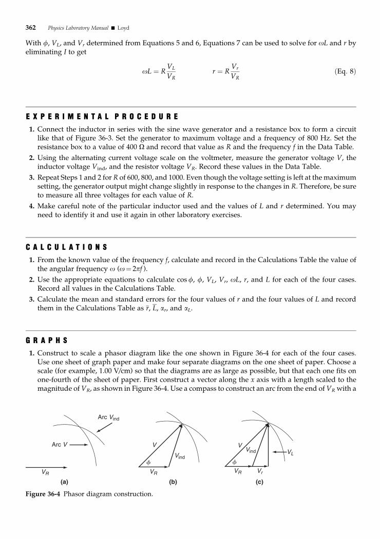
With f, VL, and Vr determined from Equations 5 and 6, Equations 7 can be used to solve for oL and r byeliminating I to get
oL ¼ RVL
VRr ¼ R
Vr
VRðEq: 8Þ
E X P E R I M E N T A L P R O C E D U R E1. Connect the inductor in series with the sine wave generator and a resistance box to form a circuit
like that of Figure 36-3. Set the generator to maximum voltage and a frequency of 800 Hz. Set theresistance box to a value of 400 O and record that value as R and the frequency f in the Data Table.
2. Using the alternating current voltage scale on the voltmeter, measure the generator voltage V, theinductor voltage Vind, and the resistor voltage VR. Record these values in the Data Table.
3. Repeat Steps 1 and 2 for R of 600, 800, and 1000. Even though the voltage setting is left at the maximumsetting, the generator output might change slightly in response to the changes in R. Therefore, be sureto measure all three voltages for each value of R.
4. Make careful note of the particular inductor used and the values of L and r determined. You mayneed to identify it and use it again in other laboratory exercises.
C A L C U L A T I O N S1. From the known value of the frequency f, calculate and record in the Calculations Table the value of
the angular frequency o (o¼ 2pf ).
2. Use the appropriate equations to calculate cosf, f, VL, Vr, oL, r, and L for each of the four cases.Record all values in the Calculations Table.
3. Calculate the mean and standard errors for the four values of r and the four values of L and recordthem in the Calculations Table as r, L, ar, and aL.
G R A P H S1. Construct to scale a phasor diagram like the one shown in Figure 36-4 for each of the four cases.
Use one sheet of graph paper and make four separate diagrams on the one sheet of paper. Choose ascale (for example, 1.00 V/cm) so that the diagrams are as large as possible, but that each one fits onone-fourth of the sheet of paper. First construct a vector along the x axis with a length scaled to themagnitude ofVR, as shown in Figure 36-4. Use a compass to construct an arc from the end of VRwith a
Arc Vind
Arc V
VR
V
Vind
VR
�
VVind
Vr
VL
VR
�
(a) (b) (c)
Figure 36-4 Phasor diagram construction.
362 Physics Laboratory Manual n Loyd

radius the length of the scaled value of Vind. Finally, construct an arc from the beginning of VR witha radius the length of the scaled value of V. The intersection of the two arcs is the intersection of Vind
and V, and those two vectors can then be drawn in their proper direction as shown in part (b) of thefigure. Finally, VL and Vr can be constructed as shown in part (c) of the figure by dropping aperpendicular from the intersection of the arcs to the x axis and extending a vector from the end of VR.
COPYRIG
HTª
2008ThomsonBrooks/Cole
Laboratory 36 n Alternating Current LR Circuits 363

This page intentionally left blank
Name . . . . . . . . . . . . . . . . . . . . . . . . . . . . . . . . . . . . . . . . . . . . . . . . . . . . . . . . . . . . . . . . . . . . . . . . . Section . . . . . . . . . . . . . . . . Date . . . . . . . . . . . . . . . .
36 L A B O R A T O R Y 3 6 Alternating Current LR Circuits
P R E - L A B O R A T O R Y A S S I G N M E N T1. For a resistor in a series alternating current circuit, the phase relationship between the current in
the resistor and the voltage across the resistor is (a) the current leads the voltage by 908 (b) the voltageleads the current by 908 (c) the current is in phase with the voltage (d) the current is at some phaseangle f relative to the voltage (f is dependent on the circuit parameters).
2. For an inductor in a series alternating current circuit, the phase relationship between the current inthe inductor and the voltage across the inductor is (a) the current leads the voltage by 908 (b) thevoltage leads the current by 908 (c) the current is in phase with the voltage (d) the current is at somephase angle f relative to the voltage (f is dependent on the circuit parameters).
3. For a generator in a series alternating current circuit, the phase relationship between the generatorvoltage and the current in the generator is (a) the current leads the voltage by 908 (b) the voltage leadsthe current by 908 (c) the current is in phase with the voltage (d) the current is at some phase angle frelative to the voltage (f is dependent on the circuit parameters).
4. If a generator has a maximum voltage of 5.00 V, what is the root-mean-square voltage of thegenerator? Show your work.
Vrms ¼ V
5. A 2.50 mH inductor has an rms voltage of 15.0 V across it at a frequency f¼ 200Hz. What is the rmscurrent in the inductor? Show your work.
Irms ¼ A
COPYRIG
HTª
2008ThomsonBrooks/Cole
365

6. A pure inductor L and a pure resistor R are in series with a generator of voltage V. The voltage acrossthe inductor is VL¼ 10.0V. The voltage across the resistor is 15.0 V. What is the voltage V of thegenerator? Show your work.
V ¼ V
7. A 500 O resistor and a real inductor with a pure inductance of L and an internal resistance of r are inseries with a generator with a voltage of V¼ 10.0V and an angular frequency of o¼ 1000 rad/s.The voltage across the real inductor is measured to be 4.73 V, and the voltage across the 500 O resistoris measured to be 6.57 V. What is the value of L and r? (Hint—This is the measurement to be per-formed in this laboratory exercise. Use the appropriate equation to find f, then the appropriateequations to find VL and Vr, and then the appropriate equations to find oL and r. Finally, find L fromthe known value of o.) Show your work.
366 Physics Laboratory Manual n Loyd

Name . . . . . . . . . . . . . . . . . . . . . . . . . . . . . . . . . . . . . . . . . . . . . . . . . . . . . . . . . . . . . . . . . . . . . . . . . Section . . . . . . . . . . . . . . . . Date . . . . . . . . . . . . . . . .
Lab Partners . . . . . . . . . . . . . . . . . . . . . . . . . . . . . . . . . . . . . . . . . . . . . . . . . . . . . . . . . . . . . . . . . . . . . . . . . . . . . . . . . . . . . . . . . . . . . . . . . . . . . . . . . . . . . . . . . . . .
36 L A B O R A T O R Y 3 6 Alternating Current LR Circuits
L A B O R A T O R Y R E P O R T
COPYRIG
HTª
2008ThomsonBrooks/Cole
Data Table
f¼ Hz
R (O)
V (V)
Vind (V)
VR (V)
Calculations Table
o¼ 2pf¼ rad/s
cosf
f (degrees)
VL (V)
Vr (V)
oL (O)
r (O)
L (H)
r ¼ O ar¼ O L ¼ H aL¼ H
367
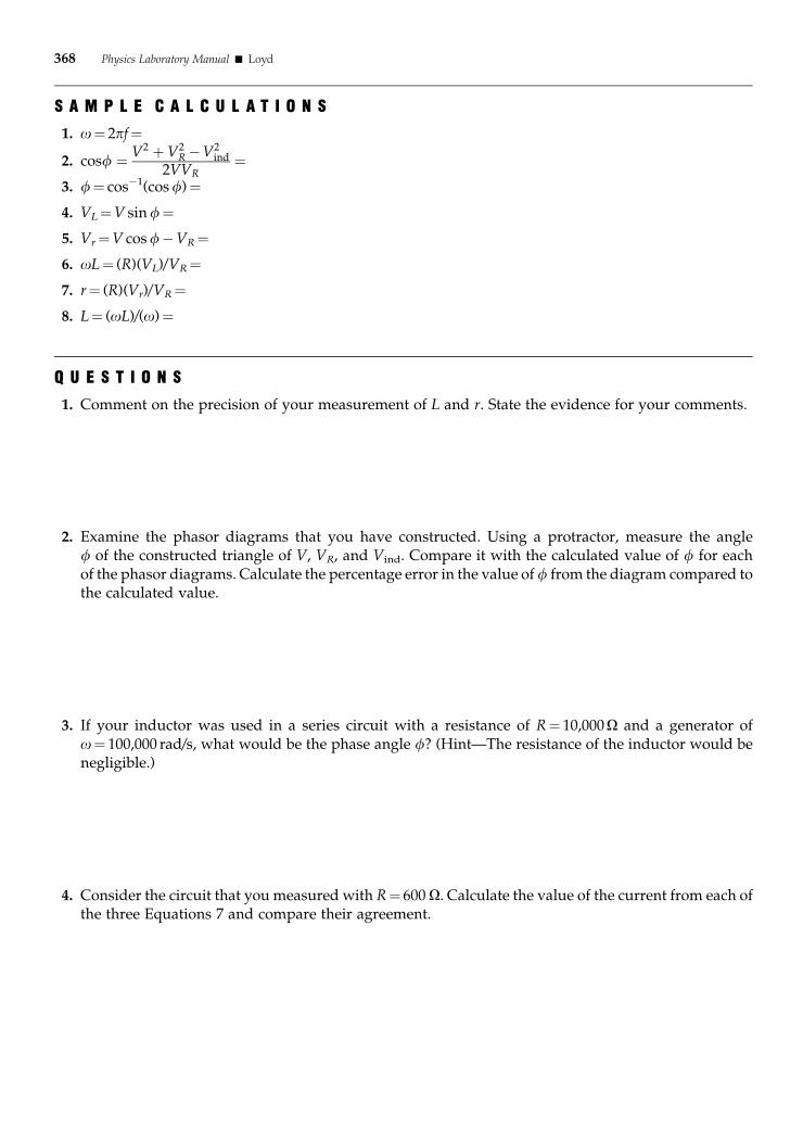
S A M P L E C A L C U L A T I O N S1. o¼ 2pf¼2. cosf ¼ V2 þ V2
R �V2ind
2VVR¼
3. f¼ cos�1(cosf)¼4. VL¼V sinf¼5. Vr¼V cosf�VR¼6. oL¼ (R)(VL)/VR¼7. r¼ (R)(Vr)/VR¼8. L¼ (oL)/(o)¼
Q U E S T I O N S1. Comment on the precision of your measurement of L and r. State the evidence for your comments.
2. Examine the phasor diagrams that you have constructed. Using a protractor, measure the anglef of the constructed triangle of V, VR, and Vind. Compare it with the calculated value of f for eachof the phasor diagrams. Calculate the percentage error in the value of f from the diagram compared tothe calculated value.
3. If your inductor was used in a series circuit with a resistance of R¼ 10,000O and a generator ofo¼ 100,000 rad/s, what would be the phase angle f? (Hint—The resistance of the inductor would benegligible.)
4. Consider the circuit that you measured with R¼ 600 O. Calculate the value of the current from each ofthe three Equations 7 and compare their agreement.
368 Physics Laboratory Manual n Loyd
Alternating Current RCand LCR Circuits
O B J E C T I V E So Investigate the phase relationship between the voltage across the resistor VR and the voltage
across the capacitor VC in an RC circuit.
o Determine the value of the capacitance of a capacitor in an RC circuit.
o Investigate the phase relationships among the voltages across the resistor, the capacitor, and theinductor in an LCR circuit.
E Q U I P M E N T L I S T. Sine wave generator (variable frequency, 5 V peak to peak amplitude), resistance box
. A 100-mH inductor of known L and r, 1.00-mF capacitor, compass, protractor
. Alternating current voltmeter (digital readout, capable of measuring high frequency)
. (This laboratory assumes that either Laboratory 36 has previously been performed, and that the values of theinductance (L) and resistance (r) for that inductor coil have been recorded and retained, or else an inductor withaccurate known values of L and r is provided.)
T H E O R YRC Circuit
A series circuit consisting of a capacitor C, a resistor R, and a sine wave generator of frequency f is shownin Figure 37-1. Also shown in the figure is a phasor diagram for the generator voltageV, the voltage acrossthe resistor VR, and the capacitor voltage VC. It is assumed that all voltages discussed in this laboratoryare root-mean-square values. The voltages VR and VC are 908 out of phase, and the voltages V, VR, and VC
form a right triangle as shown in Figure 37-1. Therefore, the equation relating the magnitudes of themeasured voltages in an RC circuit is
V ¼ffiffiffiffiffiffiffiffiffiffiffiffiffiffiffiffiffiffiV2
C þ V2R
qðEq: 1Þ
Note that Equation 1 is valid for only a pure capacitor with no resistive component. If measurements ona real capacitor show agreement with Equation 1, it would indicate that the capacitor has no significantresistive component.
Physics Laboratory Manual n Loyd L A B O R A T O R Y 37
COPYRIG
HTª
2008ThomsonBrooks/Cole
369
ª 2008 Thomson Brooks/Cole, a part of TheThomson Corporation.Thomson, the Star logo, and Brooks/Cole are trademarks used herein under license. ALL RIGHTSRESERVED.No part of this workcovered by the copyright hereonmay be reproduced or used in any form or by any meansçgraphic, electronic, ormechanical, including photocopying, recording, taping,web distribution, informationstorage and retrieval systems,or in any othermannerçwithout the written permission of the publisher.
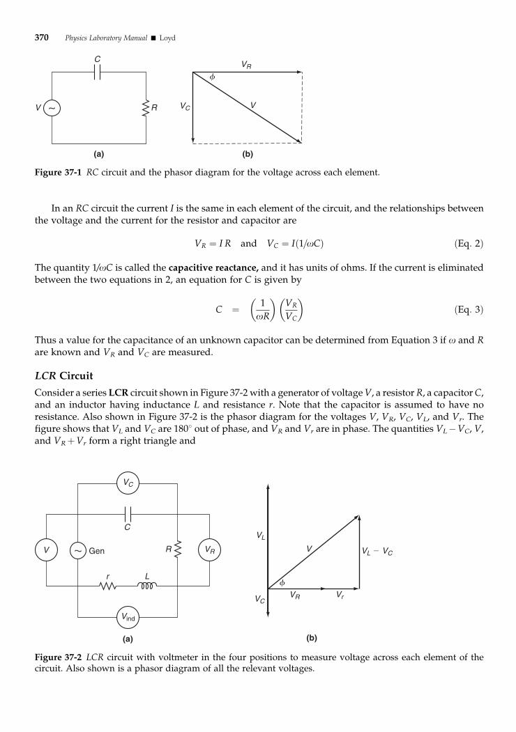
In an RC circuit the current I is the same in each element of the circuit, and the relationships betweenthe voltage and the current for the resistor and capacitor are
VR ¼ I R and VC ¼ Ið1=oCÞ ðEq: 2Þ
The quantity 1/oC is called the capacitive reactance, and it has units of ohms. If the current is eliminatedbetween the two equations in 2, an equation for C is given by
C ¼ 1
oR
� VR
VC
� ðEq: 3Þ
Thus a value for the capacitance of an unknown capacitor can be determined from Equation 3 if o and Rare known and VR and VC are measured.
LCR Circuit
Consider a series LCR circuit shown in Figure 37-2 with a generator of voltageV, a resistorR, a capacitorC,and an inductor having inductance L and resistance r. Note that the capacitor is assumed to have noresistance. Also shown in Figure 37-2 is the phasor diagram for the voltages V, VR, VC, VL, and Vr. Thefigure shows that VL and VC are 1808 out of phase, and VR and Vr are in phase. The quantities VL�VC, V,and VRþVr form a right triangle and
V VC
VR
V
C
R
(a) (b)
�
Figure 37-1 RC circuit and the phasor diagram for the voltage across each element.
VC
Vind
V
C
R
Lr
Gen VR VL � VC
VL
VCVR
V
Vr
�
(a) (b)
Figure 37-2 LCR circuit with voltmeter in the four positions to measure voltage across each element of thecircuit. Also shown is a phasor diagram of all the relevant voltages.
370 Physics Laboratory Manual n Loyd
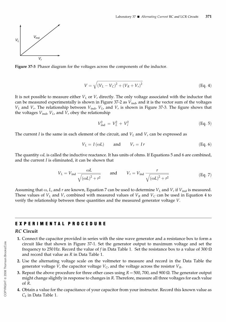
V ¼ffiffiffiffiffiffiffiffiffiffiffiffiffiffiffiffiffiffiffiffiffiffiffiffiffiffiffiffiffiffiffiffiffiffiffiffiffiffiffiffiffiffiffiffiffiffiffiffiffiffiffiffiðVL � VCÞ2 þ ðVR þ VrÞ2
qðEq: 4Þ
It is not possible to measure either VL or Vr directly. The only voltage associated with the inductor thatcan be measured experimentally is shown in Figure 37-2 as Vind, and it is the vector sum of the voltagesVL and Vr. The relationship between Vind, VL, and Vr is shown in Figure 37-3. The figure shows thatthe voltages Vind, VL, and Vr obey the relationship
V2ind ¼ V2
L þ V2r ðEq: 5Þ
The current I is the same in each element of the circuit, and VL and Vr can be expressed as
VL ¼ I ðoLÞ and Vr ¼ I r ðEq: 6Þ
The quantity oL is called the inductive reactance. It has units of ohms. If Equations 5 and 6 are combined,and the current I is eliminated, it can be shown that
VL ¼ VindoLffiffiffiffiffiffiffiffiffiffiffiffiffiffiffiffiffiffiffiffiffiffi
ðoLÞ2 þ r2q and Vr ¼ Vind
rffiffiffiffiffiffiffiffiffiffiffiffiffiffiffiffiffiffiffiffiffiffiðoLÞ2 þ r2
q ðEq: 7Þ
Assuming that o, L, and r are known, Equation 7 can be used to determine VL and Vr if Vind is measured.These values of VL and Vr combined with measured values of VR and VC can be used in Equation 4 toverify the relationship between these quantities and the measured generator voltage V.
E X P E R I M E N T A L P R O C E D U R ERC Circuit
1. Connect the capacitor provided in series with the sine wave generator and a resistance box to form acircuit like that shown in Figure 37-1. Set the generator output to maximum voltage and set thefrequency to 250Hz. Record the value of f in Data Table 1. Set the resistance box to a value of 300 Oand record that value as R in Data Table 1.
2. Use the alternating voltage scale on the voltmeter to measure and record in the Data Table thegenerator voltage V, the capacitor voltage VC, and the voltage across the resistor VR.
3. Repeat the above procedure for three other cases using R¼ 500, 700, and 900 O. The generator outputmight change slightly in response to changes in R. Therefore, measure all three voltages for each valueof R.
4. Obtain a value for the capacitance of your capacitor from your instructor. Record this known value asCk in Data Table 1.C
OPYRIG
HTª
2008ThomsonBrooks/Cole
VLVind
Vr
Figure 37-3 Phasor diagram for the voltages across the components of the inductor.
Laboratory 37 n Alternating Current RC and LCR Circuits 371
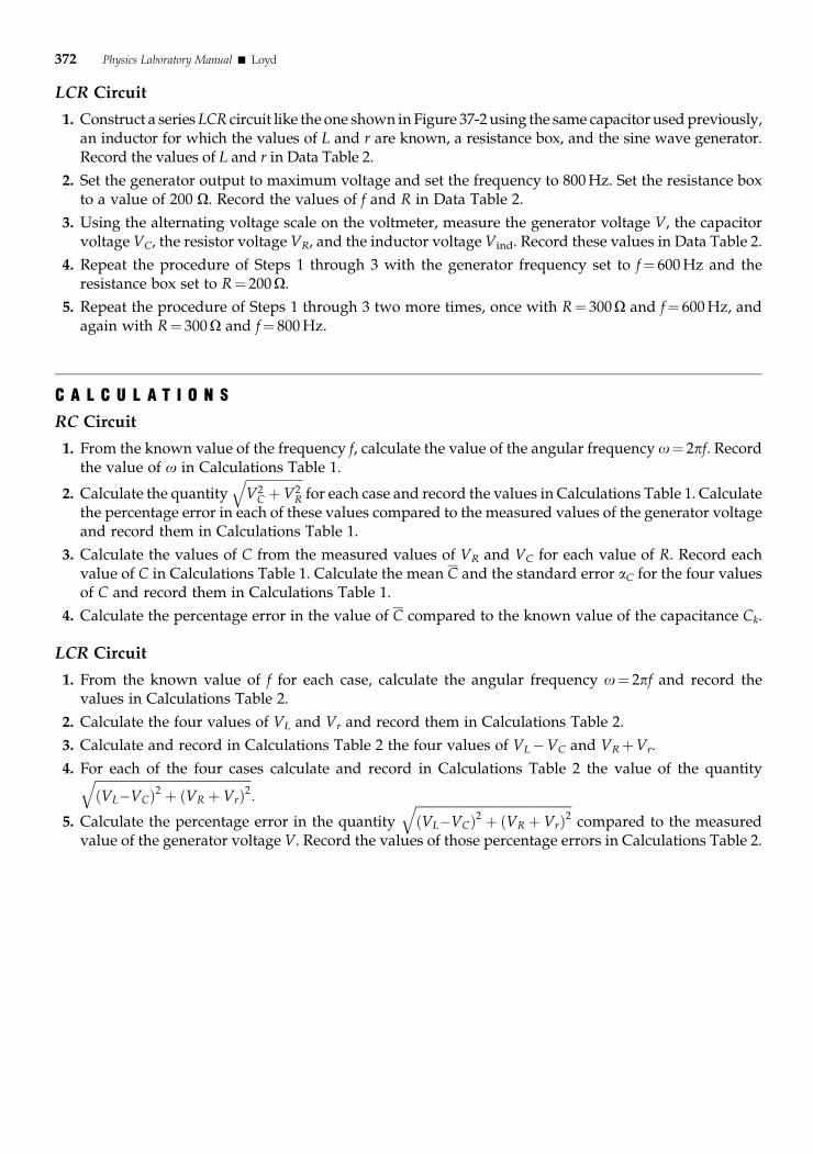
LCR Circuit
1. Construct a series LCR circuit like the one shown inFigure 37-2using the same capacitor usedpreviously,an inductor for which the values of L and r are known, a resistance box, and the sine wave generator.Record the values of L and r in Data Table 2.
2. Set the generator output to maximum voltage and set the frequency to 800Hz. Set the resistance boxto a value of 200 O. Record the values of f and R in Data Table 2.
3. Using the alternating voltage scale on the voltmeter, measure the generator voltage V, the capacitorvoltage VC, the resistor voltage VR, and the inductor voltage Vind. Record these values in Data Table 2.
4. Repeat the procedure of Steps 1 through 3 with the generator frequency set to f¼ 600Hz and theresistance box set to R¼ 200O.
5. Repeat the procedure of Steps 1 through 3 two more times, once with R¼ 300O and f¼ 600Hz, andagain with R¼ 300O and f¼ 800Hz.
C A L C U L A T I O N SRC Circuit
1. From the known value of the frequency f, calculate the value of the angular frequency o¼ 2pf. Recordthe value of o in Calculations Table 1.
2. Calculate the quantityffiffiffiffiffiffiffiffiffiffiffiffiffiffiffiffiffiffiV2
C þ V2R
qfor each case and record the values in Calculations Table 1. Calculate
the percentage error in each of these values compared to the measured values of the generator voltageand record them in Calculations Table 1.
3. Calculate the values of C from the measured values of VR and VC for each value of R. Record eachvalue of C in Calculations Table 1. Calculate the mean C and the standard error aC for the four valuesof C and record them in Calculations Table 1.
4. Calculate the percentage error in the value of C compared to the known value of the capacitance Ck.
LCR Circuit
1. From the known value of f for each case, calculate the angular frequency o¼ 2pf and record thevalues in Calculations Table 2.
2. Calculate the four values of VL and Vr and record them in Calculations Table 2.
3. Calculate and record in Calculations Table 2 the four values of VL�VC and VRþVr.
4. For each of the four cases calculate and record in Calculations Table 2 the value of the quantityffiffiffiffiffiffiffiffiffiffiffiffiffiffiffiffiffiffiffiffiffiffiffiffiffiffiffiffiffiffiffiffiffiffiffiffiffiffiffiffiffiffiffiffiffiffiffiffiffiðVL�VCÞ2 þ ðVR þ VrÞ2
q:
5. Calculate the percentage error in the quantityffiffiffiffiffiffiffiffiffiffiffiffiffiffiffiffiffiffiffiffiffiffiffiffiffiffiffiffiffiffiffiffiffiffiffiffiffiffiffiffiffiffiffiffiffiffiffiffiffiðVL�VCÞ2 þ ðVR þ VrÞ2
qcompared to the measured
value of the generator voltage V. Record the values of those percentage errors in Calculations Table 2.
372 Physics Laboratory Manual n Loyd

Name . . . . . . . . . . . . . . . . . . . . . . . . . . . . . . . . . . . . . . . . . . . . . . . . . . . . . . . . . . . . . . . . . . . . . . . . . Section . . . . . . . . . . . . . . . . Date . . . . . . . . . . . . . . . .
37 L A B O R A T O R Y 3 7 Alternating Current RC and LCR Circuits
P R E - L A B O R A T O R Y A S S I G N M E N T1. In a series RC circuit such as the one in Figure 37-1, the following phase relationship exists between
the generator voltage V, the capacitor voltage VC, and the resistor voltage VR. (a) V and VR are inphase,VC lagsVR by 908 (b)VC andVR are at angle f,V leadsVC by 908 (c)VC lagsVR by 908,V lagsVR
by angle f (d) VR lags VC by f, VC leads V by 908.
2. If a series RC circuit hasVR¼ 12.6V andVC¼ 10.7V, the generator voltagemust be (a) 12.6 V (b) 23.3 V(c) 1.9 V (d) 16.5 V. Show your work.
3. A series RC circuit has o¼ 2000 rad/s and R¼ 300O. The voltage VC is measured to be 4.76 V, and VR
is measured to be 6.78 V. What is the value of C? Show your work. (a) 2.37 mF (b) 5.00 mF (c) 1.17 mF(d) 4.67 mF.
4. A series RC circuit of R¼ 500O and C¼ 3.00mF is measured to have VR¼ 8.07V and VC¼ 6.68V. Whatis the current I, and what is the value of o the angular frequency? Show your work.
I ¼ A o¼ rad=s
COPYRIG
HTª
2008ThomsonBrooks/Cole
373

5. A series LCR circuit consists of an inductor of inductance L and resistance r, a capacitor C, a resistorR, and a generator of voltage V. Mark as true or false the following statements concerning the relativephase of V, VL, Vr, VC, and VR.
_____ 1. Vr and VR are in phase.
_____ 2. VL leads VC by 908.
_____ 3. V is at angle f relative to VR.
_____ 4. VL�VC is in phase with Vr.
_____ 5. VC lags VR by 908.
6. Measurements on the circuit described in Question 5 give VL¼ 10.76V, VC¼ 5.68V, VR¼ 6.32V, andVr¼ 3.75V. What is the generator voltage V? Show your work.
V ¼ V
7. An inductor with L¼ 150mH and r¼ 200O is in series with a capacitor, a resistor, and a generator ofo¼ 1000 rad/s. The voltage across the inductor Vind is measured to be 10.87V, VR is measured tobe 4.65V, and VC is measured to be 5.96V. What is the generator voltage V? (Hint—This is themeasurement to be performed in this laboratory for LCR circuits. Use the appropriate equations tofind VL and Vr, and then use them and the values of VR and VC to calculateV.)
374 Physics Laboratory Manual n Loyd

Name . . . . . . . . . . . . . . . . . . . . . . . . . . . . . . . . . . . . . . . . . . . . . . . . . . . . . . . . . . . . . . . . . . . . . . . . . Section . . . . . . . . . . . . . . . . Date . . . . . . . . . . . . . . . .
Lab Partners . . . . . . . . . . . . . . . . . . . . . . . . . . . . . . . . . . . . . . . . . . . . . . . . . . . . . . . . . . . . . . . . . . . . . . . . . . . . . . . . . . . . . . . . . . . . . . . . . . . . . . . . . . . . . . . . . . . .
37 L A B O R A T O R Y 3 7 Alternating Current RC and LCR Circuits
L A B O R A T O R Y R E P O R T
COPYRIG
HTª
2008ThomsonBrooks/Cole
Data Table 1
f¼ Hz Ck¼ mF
R (O)
VC (V)
VR (V)
V (V)
Calculations Table 1
o¼ rad/s
ffiffiffiffiffiffiffiffiffiffiffiffiffiffiffiffiffiffiffiV2
C þ V2R
q% Error
C (mF)
C¼ mF aC¼ mF % Error C¼
375

S A M P L E C A L C U L A T I O N S1. o ¼ 2pf¼2. V ¼
ffiffiffiffiffiffiffiffiffiffiffiffiffiffiffiffiffiffiffiV2
C þ V2R
q¼
3. C ¼ (1/oR)(VR/VC)¼4. VL ¼ ðVindÞ oL=
ffiffiffiffiffiffiffiffiffiffiffiffiffiffiffiffiffiffiffiffiffiffiðoLÞ2 þ r2
q� ¼
5. Vr ¼ ðVindÞ r=ffiffiffiffiffiffiffiffiffiffiffiffiffiffiffiffiffiffiffiffiffiffiðoLÞ2 þ r2
q� ¼
6. V ¼ffiffiffiffiffiffiffiffiffiffiffiffiffiffiffiffiffiffiffiffiffiffiffiffiffiffiffiffiffiffiffiffiffiffiffiffiffiffiffiffiffiffiffiffiffiffiffiffiffiðVL�VCÞ2 þ ðVR þ VrÞ2
q¼
Calculations Table 2
o (rad/s)
VL (V)
Vr (V)
(VL�VC) (V)
(VRþVr) (V)ffiffiffiffiffiffiffiffiffiffiffiffiffiffiffiffiffiffiffiffiffiffiffiffiffiffiffiffiffiffiffiffiffiffiffiffiffiffiffiffiffiffiffiffiffiffiffiðVL�VCÞ2 þ ðVR�VrÞ2
qðVÞ
% Error compared to V
Data Table 2
r¼ O L¼ H C¼ mF
f (Hz)
R (O)
V (V)
Vind (V)
VC (V)
VR (V)
376 Physics Laboratory Manual n Loyd
Q U E S T I O N S1. Comment on the agreement between the measured generator voltage V and the quantity
ffiffiffiffiffiffiffiffiffiffiffiffiffiffiffiffiffiffiV2
C þ V2R
qfor the RC circuit data.
2. Do your results for Question 1 confirm that the capacitor has no resistance? State specifically how thedata either do or do not confirm this expectation.
3. State carefully your evaluation of the precision of your measurements of the value of the capacitorin the RC circuit. State the evidence for your opinion.
4. Considering the given value of Ck as the true value, comment on the accuracy of your measurementsof the capacitance.
5. Comment on the agreement between the measured generator voltage V and the quantityffiffiffiffiffiffiffiffiffiffiffiffiffiffiffiffiffiffiffiffiffiffiffiffiffiffiffiffiffiffiffiffiffiffiffiffiffiffiffiffiffiffiffiffiffiffiffiffiffiðVL�VCÞ2 þ ðVR þ VrÞ2
qin the LCR circuit.
COPYRIG
HTª
2008ThomsonBrooks/Cole
Laboratory 37 n Alternating Current RC and LCR Circuits 377

6. Do your results confirm the phasor diagram of Figure 37-2 as a correct model for the addition of thevoltages in an LCR circuit? State why they do or do not confirm this model.
378 Physics Laboratory Manual n Loyd
Oscilloscope Measurements
O B J E C T I V E So Investigate the fundamental principles and practical operation of the oscilloscope using signals
from a function generator.
o Measure sine and other waveform signals of varying voltage and frequency.
o Compare voltage measurements with the oscilloscope to voltage measurements using an alter-nating current voltmeter.
E Q U I P M E N T L I S T. Oscilloscope (typical direct current to 20Mhz), alternating current voltmeter (high frequency capability)
. Function generator (sine wave plus additional wave form such as a square wave or triangular wave),appropriate connecting wires (BNC to banana plug)
T H E O R YThe fundamental working part of an oscilloscope is a device called a cathode-ray tube (CRT). Its com-ponents include a heated filament to emit a beam of electrons, a series of electrodes to accelerate, focus,and control the intensity of the emitted electrons, two pairs of deflection plates that deflect the electronbeam when there is a voltage between the plates (one pair for deflection in the horizontal direction andone pair for deflection in the vertical direction), and a fluorescent screen that emits a visible spot of lightat the point where the beam of electrons strikes the screen. Together the heated filament and series ofelectrodes are called an electron gun. The electron gun and deflecting plates are arranged linearly insidean evacuated glass tube, and the fluorescent screen coats the glass tube at the opposite end of the tubefrom the electron gun as shown in Figure 38-1.
When there is no voltage between either pair of deflection plates, the electron beamwill travel straightdown the evacuated tube and strike the center of the fluorescent screen.When a constant voltage is appliedbetween either the horizontal or vertical deflection plates, the beamwill be displaced by a constant amounton the fluorescent screen in either the horizontal (x) or vertical (y) direction. The direction of the displa-cement depends upon the sign of the voltage, and the magnitude of the displacement is proportional tothe voltage. If a time-varying voltage is applied to either set of deflecting plates, the displacement of thebeam will vary with time as the applied voltage varies with time, and the electron beam spot will moveon the screen as a function of time. When the beam strikes the screen the phosphor glow persists forapproximately 0.1 s.
Physics Laboratory Manual n Loyd L A B O R A T O R Y 38
COPYRIG
HTª
2008ThomsonBrooks/Cole
379
ª 2008 Thomson Brooks/Cole, a part of TheThomson Corporation.Thomson, the Star logo, and Brooks/Cole are trademarks used herein under license. ALL RIGHTSRESERVED.No part of this workcovered by the copyright hereonmay be reproduced or used in any form or by any meansçgraphic, electronic, ormechanical, including photocopying, recording, taping,web distribution, informationstorage and retrieval systems,or in any othermannerçwithout the written permission of the publisher.
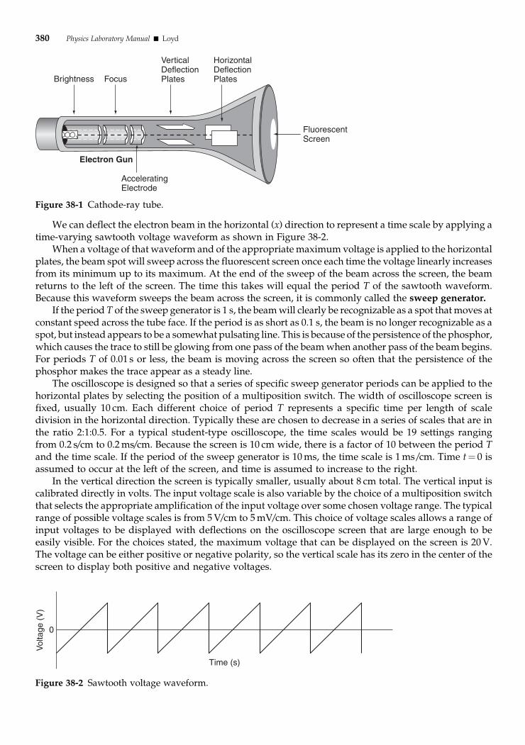
We can deflect the electron beam in the horizontal (x) direction to represent a time scale by applying atime-varying sawtooth voltage waveform as shown in Figure 38-2.
When a voltage of that waveform and of the appropriatemaximumvoltage is applied to the horizontalplates, the beam spot will sweep across the fluorescent screen once each time the voltage linearly increasesfrom its minimum up to its maximum. At the end of the sweep of the beam across the screen, the beamreturns to the left of the screen. The time this takes will equal the period T of the sawtooth waveform.Because this waveform sweeps the beam across the screen, it is commonly called the sweep generator.
If the period T of the sweep generator is 1 s, the beamwill clearly be recognizable as a spot thatmoves atconstant speed across the tube face. If the period is as short as 0.1 s, the beam is no longer recognizable as aspot, but instead appears to be a somewhat pulsating line. This is because of the persistence of the phosphor,which causes the trace to still be glowing from one pass of the beamwhen another pass of the beam begins.For periods T of 0.01 s or less, the beam is moving across the screen so often that the persistence of thephosphor makes the trace appear as a steady line.
The oscilloscope is designed so that a series of specific sweep generator periods can be applied to thehorizontal plates by selecting the position of a multiposition switch. The width of oscilloscope screen isfixed, usually 10 cm. Each different choice of period T represents a specific time per length of scaledivision in the horizontal direction. Typically these are chosen to decrease in a series of scales that are inthe ratio 2:1:0.5. For a typical student-type oscilloscope, the time scales would be 19 settings rangingfrom 0.2 s/cm to 0.2ms/cm. Because the screen is 10 cm wide, there is a factor of 10 between the period Tand the time scale. If the period of the sweep generator is 10ms, the time scale is 1ms/cm. Time t¼ 0 isassumed to occur at the left of the screen, and time is assumed to increase to the right.
In the vertical direction the screen is typically smaller, usually about 8 cm total. The vertical input iscalibrated directly in volts. The input voltage scale is also variable by the choice of a multiposition switchthat selects the appropriate amplification of the input voltage over some chosen voltage range. The typicalrange of possible voltage scales is from 5V/cm to 5mV/cm. This choice of voltage scales allows a range ofinput voltages to be displayed with deflections on the oscilloscope screen that are large enough to beeasily visible. For the choices stated, the maximum voltage that can be displayed on the screen is 20V.The voltage can be either positive or negative polarity, so the vertical scale has its zero in the center of thescreen to display both positive and negative voltages.
Brightness Focus
VerticalDeflectionPlates
AcceleratingElectrode
Electron Gun
HorizontalDeflectionPlates
FluorescentScreen
Figure 38-1 Cathode-ray tube.
0
Time (s)
Vol
tage
(V
)
Figure 38-2 Sawtooth voltage waveform.
380 Physics Laboratory Manual n Loyd
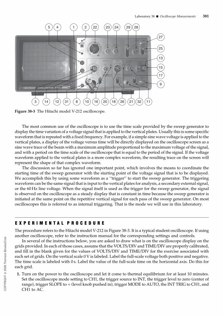
The most common use of the oscilloscope is to use the time scale provided by the sweep generator todisplay the time variation of a voltage signal that is applied to the vertical plates. Usually this is some specificwaveform that is repeatedwith a fixed frequency. For example, if a simple sinewave voltage is applied to thevertical plates, a display of the voltage versus time will be directly displayed on the oscilloscope screen as asinewave trace of the beamwith amaximum amplitude proportional to themaximumvoltage of the signal,and with a period on the time scale of the oscilloscope that is equal to the period of the signal. If the voltagewaveform applied to the vertical plates is a more complex waveform, the resulting trace on the screen willrepresent the shape of that complex waveform.
The discussion so far has ignored one important point, which involves the means to coordinate thestarting time of the sweep generator with the starting point of the voltage signal that is to be displayed.We accomplish this by using some waveform as a ‘‘trigger’’ to start the sweep generator. The triggeringwaveform can be the same signal that is input to the vertical plates for analysis, a secondary external signal,or the 60Hz line voltage. When the signal itself is used as the trigger for the sweep generator, the signalis observed on the oscilloscope as a steady display that is constant in time because the sweep generator isinitiated at the same point on the repetitive vertical signal for each pass of the sweep generator. On mostoscilloscopes this is referred to as internal triggering. That is the mode we will use in this laboratory.
E X P E R I M E N T A L P R O C E D U R EThe procedure refers to the Hitachi model V-212 in Figure 38-3. It is a typical student oscilloscope. If usinganother oscilloscope, refer to the instruction manual for the corresponding settings and controls.
In several of the instructions below, you are asked to draw what is on the oscilloscope display on thegrids provided. In each of those cases, assume that the VOLTS/DIV and TIME/DIV are properly calibrated,and fill in the blank given for the values of VOLTS/DIV and TIME/DIV for the exercise associated witheach set of grids. On the vertical scale 0V is labeled. Label the full-scale voltage both positive and negative.The time scale is labeled with 0 s. Label the value of the full-scale time on the horizontal axis. Do this foreach grid.
1. Turn on the power to the oscilloscope and let it come to thermal equilibrium for at least 10 minutes.Set the oscilloscope mode setting to CH1, the trigger source to INT, the trigger level to zero (center ofrange), trigger SLOPE toþ (level knob pushed in), trigger MODE to AUTO, the INT TRIG to CH1, andCH1 to AC.C
OPYRIG
HTª
2008ThomsonBrooks/Cole
5 4 1 2 22 23 24 29 28
27
25
13
15
9
11
17
3226 211820161083112143
Figure 38-3 The Hitachi model V-212 oscilloscope.
Laboratory 38 n Oscilloscope Measurements 381
2. Set the TIME/DIV control to 1ms/DIV, the SWP VAR control rotated fully clockwise to the CALposition, the VOLTS/DIV control to 1 V/DIV, and the VAR (PULL� 5 GAIN) control rotated fullyclockwise to the CAL position.
3. Turn on the power to the function generator and let it come to thermal equilibrium for at least10 minutes. Select a sine wave voltage, set the frequency f¼ 100Hz, and connect the output of thefunction generator to the CH1 INPUT of the oscilloscope. Adjust the amplitude control of the functiongenerator to zero. Adjust the VERTICAL POSITION control of the oscilloscope until the flat trace isexactly on the center line of the vertical display.
4. (a) Adjust the amplitude control of the function generator until the display on the oscilloscope is full-scale positive on the positive part of the cycle and full-scale negative on the negative part of the cycle.In the laboratory report section, carefully draw on the grid labeled 1Awhat is displayed on the screen.(b) Leaving all other parameters fixed, set the VOLT/DIV control to 2V/DIV, and draw on the gridlabeled 1Bwhat is nowdisplayedon the screen. (c) Leaving all otherparameters fixed, set theVOLT/DIVcontrol to 5V/DIV, and draw on the grid labeled 1C what is now displayed on the screen.
5. (a) Leaving all other parameters fixed, set the VOLT/DIV control to 1 V/DIV, and select f¼ 200Hz fromthe function generator. Draw on the grid labeled 2Awhat is nowdisplayed on the screen. (b) Leaving allother parameters fixed, select f¼ 400Hz from the function generator, and draw on the grid labeled 2Bwhat is now displayed on the screen. (c) Leaving all other parameters fixed, select f¼ 600Hz from thefunction generator, and draw on the grid labeled 2C what is now displayed on the screen.
6. (a) Leaving all other parameters fixed, set the VOLT/DIV control to 1 V/DIV, the TIME/DIV control to2ms/DIV, and select f¼ 100Hz from the function generator. Note that the trigger slope control is stillset at (þ). Draw on the grid labeled 3A what is now displayed on the screen. (b) Leaving all otherparameters fixed, pull out the trigger level control that sets the trigger slope to (�). Draw on the gridlabeled 3B what is now displayed on the screen.
7. (a) Leaving all other parameters fixed, push in the trigger level control that sets the trigger slope to (þ),and the trigger level is still set at zero. Draw on the grid label 4A what is now displayed on the screen.(b) Leaving all other parameters fixed, slowly turn the trigger level control clockwise, increasingthe trigger level. Increase it only so long as the display remains triggered.At themaximum level that thedisplay is triggered, draw on the grid labeled 4B what is displayed on the screen. (c) Leaving all otherparameters fixed, slowly turn the trigger level control counterclockwise, decreasing the trigger level.Decrease it only so long as the display remains triggered. At the minimum level that the display istriggered, draw on the grid labeled 4C what is displayed on the screen.
8. Push the trigger level control in for (þ) slope and turn the level back to zero. Set the TIME/DIV to2ms/DIV and set the function generator to a sine wave of f¼ 100Hz. Use the alternating currentvoltmeter to set the output of the function generator to 1.00V as read on the voltmeter. Input this sinewave to the oscil-loscope andmeasure the peak voltage of the sine wave. Tomeasure the peak voltage ofthe sine wave, you are free to adjust the VOLT/DIV control to give the most accurate measurementpossible. Generally this means adjusting the scale for as large a deflection as possible. Record the peakvoltage of the sine wave as read from the oscilloscope in Data Table 1. Complete all themeasurements inDataTable 1 from1.00V to 5.00V. For eachvoltage, set the output from the generator using the voltmeter,and then read the voltage from the oscilloscope, each time choosing the VOLT/DIV that will allow themost accurate reading from the oscilloscope.
9. Set the function generator to output a triangular wave with f¼ 1000Hz, and the TIME/DIV on theoscilloscope to 1ms/DIV. Use the alternating current voltmeter to set the output of the functiongenerator to 1.00V as read on the voltmeter. Input this triangular wave to the oscilloscope andmeasurethe peak voltage of the wave. Proceed as instructed for the sine wave above, this time measuring thevoltages between 1.00V and 5.00V as read on the voltmeter. Record the results in Data Table 2.
382 Physics Laboratory Manual n Loyd

10. The goal of this laboratory is to introduce students to the oscilloscope. Now simply experiment foryourself with the features of the oscilloscope. Input as many different frequencies and waveforms astime allows and attempt to learn everything you can about the operation of the oscilloscope by simplytrying different settings of all of the oscilloscope controls.
C A L C U L A T I O N S1. Perform a linear least squares fit to the data in Data Table 1 with the peak voltage read on the oscillo-
scope as the horizontal axis and the voltage as read on the voltmeter as the vertical axis. Determine theslope, the intercept, and the correlation coefficient. Record those values in Calculations Table 1.
2. Performa linear least squares fit to thedata inDataTable 2with thepeakvoltage readon theoscilloscopeas the horizontal axis and the voltage as read on the voltmeter as the vertical axis. Determine the slope,the intercept, and the correlation coefficient. Record those values in Calculations Table 2.
COPYRIG
HTª
2008ThomsonBrooks/Cole
Laboratory 38 n Oscilloscope Measurements 383

This page intentionally left blank
Name . . . . . . . . . . . . . . . . . . . . . . . . . . . . . . . . . . . . . . . . . . . . . . . . . . . . . . . . . . . . . . . . . . . . . . . . . Section . . . . . . . . . . . . . . . . Date . . . . . . . . . . . . . . . .
38 L A B O R A T O R Y 3 8 Oscilloscope Measurements
P R E - L A B O R A T O R Y A S S I G N M E N T1. Describe the components that make up the electron gun in a cathode-ray tube.
2. Describe the voltage waveform that produces a linear time scale when applied to the horizontal platesof a cathode-ray tube.
3. When the electron beam strikes the fluorescent screen, the phosphor glow that results has persistence.Approximately how long does the glow persist?
4. A function generator outputs a sine wave of f¼ 200Hz. It is input to an oscilloscope set at 1ms/DIV.How many complete cycles of the sine wave are displayed on the oscilloscope? (Hint—The period ofthe sine wave T is related to the frequency f of the wave by T¼ 1/f, and there are 10 divisions on thetime display of the oscilloscope.)
COPYRIG
HTª
2008ThomsonBrooks/Cole
385

5. A typical student oscilloscope on its least sensitive calibrated scale can display a voltage up to amaximum of approximately (a) 1V (b) 5V (c) 20V (d) 200V.
6. A typical student oscilloscope on its most sensitive calibrated scale can display a voltage down to aminimum of approximately (a) 1mV (b) 5mV (c) 20V (d) 200mV.
7. A sawtooth wave with a period of 100ms is applied to an oscilloscope with a screen 10 cm wide.What time is represented by 1 cm on the screen?
386 Physics Laboratory Manual n Loyd

Name . . . . . . . . . . . . . . . . . . . . . . . . . . . . . . . . . . . . . . . . . . . . . . . . . . . . . . . . . . . . . . . . . . . . . . . . . Section . . . . . . . . . . . . . . . . Date . . . . . . . . . . . . . . . .
Lab Partners . . . . . . . . . . . . . . . . . . . . . . . . . . . . . . . . . . . . . . . . . . . . . . . . . . . . . . . . . . . . . . . . . . . . . . . . . . . . . . . . . . . . . . . . . . . . . . . . . . . . . . . . . . . . . . . . . . . .
38 L A B O R A T O R Y 3 8 Oscilloscope Measurements
L A B O R A T O R Y R E P O R T
1A. TIME/DIV= __________ 1B. TIME/DIV=__________ 1C. TIME/DIV=__________
1A. VOLTS/DIV=__________ 1B. VOLTS/DIV=__________ 1C. VOLTS/DIV=__________
0 V
0 s
0 V
0 s
0 V
0 s
2A. TIME/DIV= __________ 2B. TIME/DIV=__________ 2C. TIME/DIV=__________
2A. VOLTS/DIV=__________ 2B. VOLTS/DIV=__________ 2C. VOLTS/DIV=__________
0 V
0 s
0 V
0 s
0 V
0 s
3A. TIME/DIV= __________ 3B. TIME/DIV=__________
3A. VOLTS/DIV=__________ 3B. VOLTS/DIV=__________
0 V
0 s
0 V
0 s
COPYRIG
HTª
2008ThomsonBrooks/Cole
387
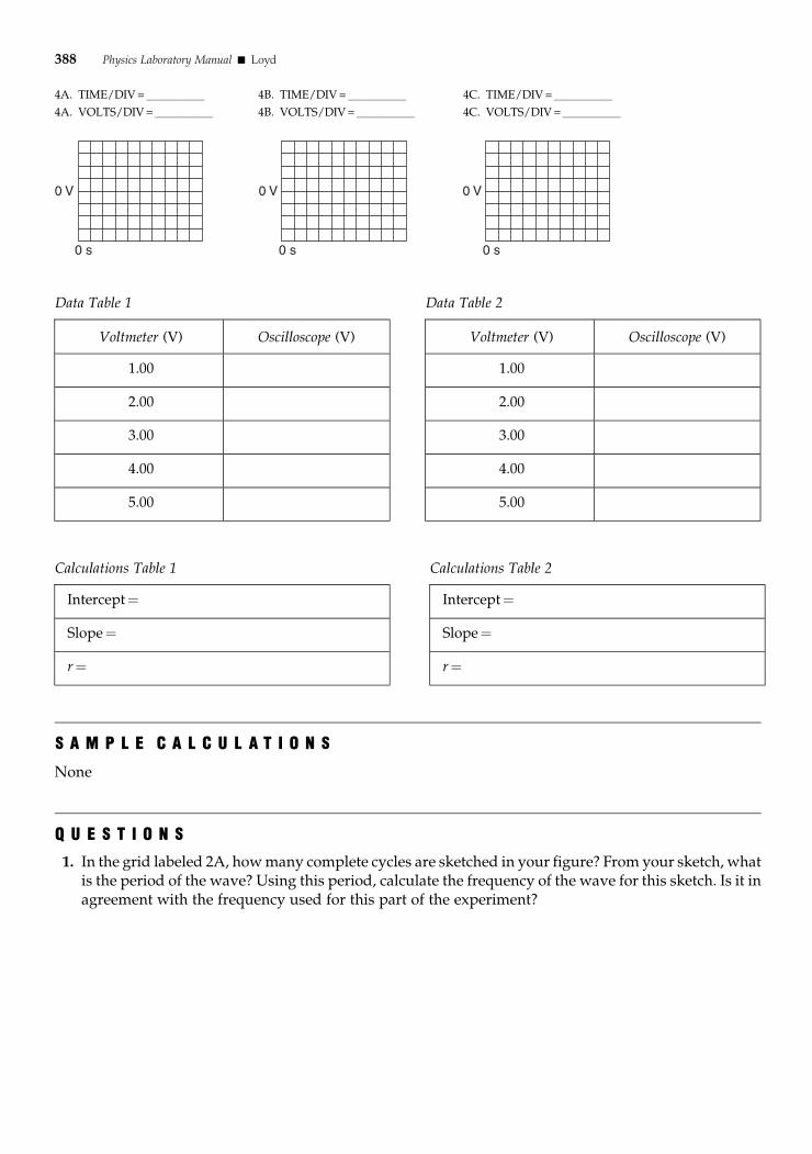
4A. TIME/DIV=__________ 4B. TIME/DIV=__________ 4C. TIME/DIV=__________
4A. VOLTS/DIV=__________ 4B. VOLTS/DIV=__________ 4C. VOLTS/DIV=__________
0 V
0 s
0 V
0 s
0 V
0 s
S A M P L E C A L C U L A T I O N S
None
Q U E S T I O N S1. In the grid labeled 2A, howmany complete cycles are sketched in your figure? From your sketch, what
is the period of the wave? Using this period, calculate the frequency of the wave for this sketch. Is it inagreement with the frequency used for this part of the experiment?
Data Table 1
Voltmeter (V) Oscilloscope (V)
1.00
2.00
3.00
4.00
5.00
Data Table 2
Voltmeter (V) Oscilloscope (V)
1.00
2.00
3.00
4.00
5.00
Calculations Table 1
Intercept¼
Slope¼
r¼
Calculations Table 2
Intercept¼
Slope¼
r¼
388 Physics Laboratory Manual n Loyd
2. In your own words, explain why these two sketches in 3A and 3B appear as they do. They both havethe trigger level zero, but one has a positive trigger slope and the other has a negative trigger slope.
3. Explain the appearance of sketches 4A, 4B, and 4C. They all have a positive trigger slope, but thetrigger level of 4A is zero, the trigger level of 4B is positive, and the trigger level of 4C is negative.
4. For a sine wave, an alternating current voltmeter measures a root-mean-square value that is 0.707 ofthe peak value of the sine wave. Therefore the peak value measured on the oscilloscope should be1/.707, or 1.414 times the voltmeter readings. The slope of the data in Data Table 1 that you calculatedand recorded in Calculations Table 1 should be approximately 1.414. Calculate the percentage errorbetween your slope for these data and 1.414.
5. For a triangular wave, an alternating current voltmeter measures a root-mean-square value that is0.576 of the peak value of the triangular wave. Therefore the peak value measured on the oscilloscopeshould be 1/.576, or 1.736 times the voltmeter readings. The slope of the data in Data Table 2 that youcalculated and recorded in Calculations Table 2 should be approximately 1.736. Calculate thepercentage error between your slope for these data and 1.736.
6. An oscilloscope is set on a TIME/DIV setting of 50ms. There are 10 divisions on the time scale. A sinewave on the oscilloscope display has exactly three full cycles of the sine wave that fit on the 10divisions. What is the frequency of the wave?
COPYRIG
HTª
2008ThomsonBrooks/Cole
Laboratory 38 n Oscilloscope Measurements 389

This page intentionally left blank
Joule Heating of a Resistor
O B J E C T I V E So Investigate the dependence of the rise in temperature on the electrical energy input when an
electric coil is immersed in water in a calorimeter.
o Determine an experimental value for the quantity commonly known as the mechanicalequivalent of heat (MEH) and compare that value to the known value.
E Q U I P M E N T L I S T. Immersion heater coil to fit standard calorimeter, calorimeter, thermometer
. Direct current power supply (5A at 6 V), ammeter (0–5A), voltmeter (0–10 V)
. Laboratory timer, laboratory balance, calibrated masses
T H E O R YWhen a resistor of resistance R has a current I at voltage V the power absorbed in the resistor is
P ¼ I2R ¼ V2=R ¼ V I ðEq: 1Þ
Power is energy per unit time, and if the power P is constant, the energy U delivered in time t is given by
U ¼ Pt ðEq: 2Þ
Substituting Equation 1 into Equation 2 gives the following expression for the electrical energy
U ¼ VI t ðEq: 3Þ
When a resistor absorbs electrical energy, it dissipates this energy in the form of heat Q. If the resistor isplaced in a calorimeter, the amount of heat produced can be measured when it is absorbed in thecalorimeter. Consider the experimental arrangement shown in Figure 39-1 in which a resistor coil (alsocalled an immersion heater) is immersed in the water in a calorimeter. The heatQ produced in the resistoris absorbed by the water, the calorimeter cup, and the resistor coil itself. This heat Q produces a rise intemperature DT. The heat Q is related to DT by
Q ¼ ðmwcw þmccc þmrcrÞDT ðEq: 4Þ
Physics Laboratory Manual n Loyd L A B O R A T O R Y 39
COPYRIG
HTª
2008ThomsonBrooks/Cole
391
ª 2008 Thomson Brooks/Cole, a part of TheThomson Corporation.Thomson, the Star logo, and Brooks/Cole are trademarks used herein under license. ALL RIGHTSRESERVED.No part of this workcovered by the copyright hereonmay be reproduced or used in any form or by any meansçgraphic, electronic, ormechanical, including photocopying, recording, taping,web distribution, informationstorage and retrieval systems,or in any othermannerçwithout the written permission of the publisher.
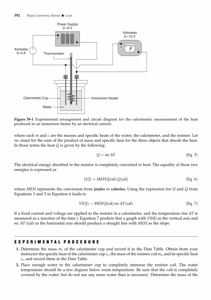
where each m and c are the masses and specific heats of the water, the calorimeter, and the resistor. Letmc stand for the sum of the product of mass and specific heat for the three objects that absorb the heat.In those terms the heat Q is given by the following:
Q ¼ mcDT ðEq: 5Þ
The electrical energy absorbed in the resistor is completely converted to heat. The equality of those twoenergies is expressed as
UðJÞ ¼ MEHðJ=calÞQðcalÞ ðEq: 6Þ
where MEH represents the conversion from joules to calories. Using the expression for U and Q fromEquations 3 and 5 in Equation 6 leads to
VItðJÞ ¼ MEHðJ=calÞmcDTðcalÞ ðEq: 7Þ
If a fixed current and voltage are applied to the resistor in a calorimeter, and the temperature rise DT ismeasured as a function of the time t, Equation 7 predicts that a graph with VIt(J) as the vertical axis andmc DT (cal) as the horizontal axis should produce a straight line with MEH as the slope.
E X P E R I M E N T A L P R O C E D U R E1. Determine the mass mc of the calorimeter cup and record it in the Data Table. Obtain from your
instructor the specific heat of the calorimeter cup cc, themass of the resistor coilmr, and its specific heatcr, and record them in the Data Table.
2. Place enough water in the calorimeter cup to completely immerse the resistor coil. The watertemperature should be a few degrees below room temperature. Be sure that the coil is completelycovered by the water, but do not use any more water than is necessary. Determine the mass of the
Ammeter0–5 A Thermometer
Calorimeter Cup
Water
Immersion Heater
Power Supply0–6 V
Voltmeter0–10 V�
� �
���
�
Figure 39-1 Experimental arrangement and circuit diagram for the calorimetric measurement of the heatproduced in an immersion heater by an electrical current.
392 Physics Laboratory Manual n Loyd
water plus the calorimeter cup and record it in the Data Table. Determine the mass of the water bysubtraction and record it as mw in the Data Table.
3. Place the immersion heater in the calorimeter cup and construct the circuit shown in Figure 39-1.Check again that the immersion heater is below the water level. If it is not, add some more water anddetermine the mass of the water again.
4. Turn on the power supply and adjust the current between 4.0 and 5.0 A. Do this quickly and then turnoff the supply with the output level still adjusted to the setting that produced the desired current.Do not allow the supply to stay on long enough to heat the water appreciably. Stir the system severalminutes to allow it to come to equilibrium.
5. Determine the initial temperature Ti and record it in the Data Table. Estimate the thermometerreadings to the nearest 0.1 C8 for all temperature measurements.
6. With the power supply still set to the output level required to produce 4.0 A, turn on the power supplyand simultaneously start the laboratory timer. Record the initial values of the current I and the voltageV in the Data Table. Let the timer run continuously and stir the system often. Measure and recordthe temperature T, the current I, and the voltage V every 60 s for 8 minutes. Record all data in theData Table.
C A L C U L A T I O N S1. Calculate the quantity mc where mc¼mwcwþmcccþmrcr and record it in the Calculations Table.
2. Calculate the temperature rise DT above the initial temperature Ti from DT¼T�Ti for each of themeasured values of T and record the results in the Calculations Table.
3. Calculate the quantity mc DT for each case and record the results in the Calculations Table.
4. For eachmeasurement of the voltageV and current I, calculate the productVI and record the results inthe Calculations Table.
5. Calculate the mean VI and standard error aVI for the values of VI and record the results in theCalculations Table.
6. Calculate the quantity VI t for each time t and record the results in the Calculations Table.
7. Perform a linear least squares fit to the data with VI t as the vertical axis and mc DT as the horizontalaxis. Determine the slopeMEHexp, the intercept A, and the correlation coefficient r and record them inthe Calculations Table.
8. Calculate the percentage error in the value of MEHexp compared to the known value of MEH¼ 4.186 J/cal.
G R A P H S1. Graph the data with VI t as the vertical axis and mc DT as the horizontal axis. Also show on the graph
the straight line obtained from the linear least squares fit.
COPYRIG
HTª
2008ThomsonBrooks/Cole
Laboratory 39 n Joule Heating of a Resistor 393

This page intentionally left blank
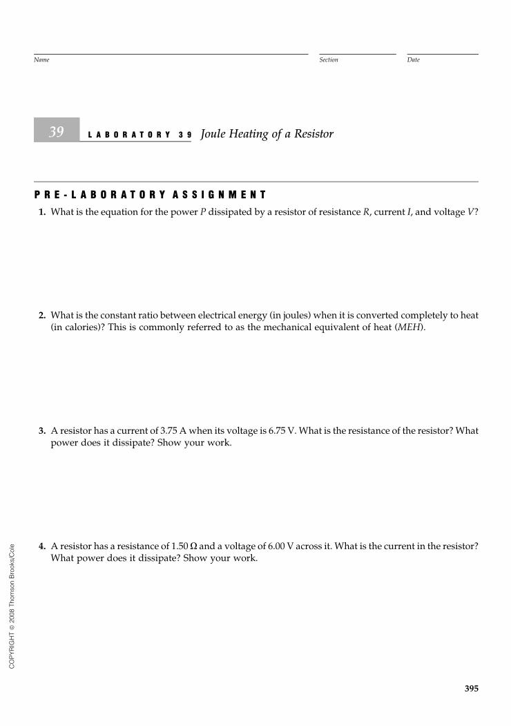
Name . . . . . . . . . . . . . . . . . . . . . . . . . . . . . . . . . . . . . . . . . . . . . . . . . . . . . . . . . . . . . . . . . . . . . . . . . Section . . . . . . . . . . . . . . . . Date . . . . . . . . . . . . . . . .
39 L A B O R A T O R Y 3 9 Joule Heating of a Resistor
P R E - L A B O R A T O R Y A S S I G N M E N T1. What is the equation for the power P dissipated by a resistor of resistance R, current I, and voltage V?
2. What is the constant ratio between electrical energy (in joules) when it is converted completely to heat(in calories)? This is commonly referred to as the mechanical equivalent of heat (MEH).
3. A resistor has a current of 3.75 Awhen its voltage is 6.75 V.What is the resistance of the resistor?Whatpower does it dissipate? Show your work.
4. A resistor has a resistance of 1.50O and a voltage of 6.00 V across it. What is the current in the resistor?What power does it dissipate? Show your work.
COPYRIG
HTª
2008ThomsonBrooks/Cole
395

5. If the resistor in Question 4 is immersed in water, how much energy does it deliver to the water in350 s? Express your answer in joules and in calories. Show your work.
6. A resistor has a voltage of 6.65 V and a current of 4.45 A. It is placed in a calorimeter containing 200 gof water at 24.08C. The calorimeter is aluminum (specific heat¼ 0.220 cal/g–C8), and its mass is 60.0 g.The heat capacity of the resistor itself is negligible. What is the temperature of the system 500 s laterif all the electrical energy goes into heating the water and the calorimeter? Show your work.
396 Physics Laboratory Manual n Loyd

Name . . . . . . . . . . . . . . . . . . . . . . . . . . . . . . . . . . . . . . . . . . . . . . . . . . . . . . . . . . . . . . . . . . . . . . . . . Section . . . . . . . . . . . . . . . . Date . . . . . . . . . . . . . . . .
Lab Partners . . . . . . . . . . . . . . . . . . . . . . . . . . . . . . . . . . . . . . . . . . . . . . . . . . . . . . . . . . . . . . . . . . . . . . . . . . . . . . . . . . . . . . . . . . . . . . . . . . . . . . . . . . . . . . . . . . . .
39 L A B O R A T O R Y 3 9 Joule Heating of a Resistor
L A B O R A T O R Y R E P O R T
COPYRIG
HTª
2008ThomsonBrooks/Cole
Data Table
Mass calorimeterþwater g Ti¼ 8C
Mass calorimeter g c of calorimeter¼ cal/g�C8
Mass water g c of water cal/g�C8
Mass resistor coil g c of resistor coil cal/g�C8
t (s) V (V) I (A) T (8C)
0
60
120
180
240
300
360
420
480
397
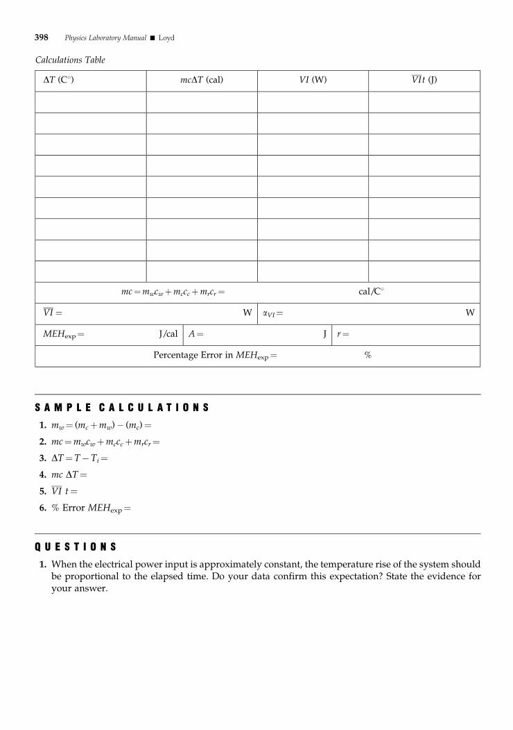
S A M P L E C A L C U L A T I O N S1. mw¼ (mcþmw)� (mc)¼2. mc¼mwcwþmcccþmrcr¼3. DT¼T�Ti¼4. mc DT¼5. VI t¼6. % Error MEHexp¼
Q U E S T I O N S1. When the electrical power input is approximately constant, the temperature rise of the system should
be proportional to the elapsed time. Do your data confirm this expectation? State the evidence foryour answer.
Calculations Table
DT (C8) mcDT (cal) VI (W) VIt (J)
mc¼mwcwþmcccþmrcr¼ cal/C8
VI ¼ W aVI¼ W
MEHexp¼ J/cal A¼ J r¼
Percentage Error in MEHexp¼ %
398 Physics Laboratory Manual n Loyd

2. What is the accuracy of your experimental value for MEH? State your evidence.
3. How long from the original starting time would it have taken to achieve a temperature of 50.08C withthe experimental arrangement you used? Show your work.
4. Assuming that one used the same heating coil and that its resistance did not change, howmuchwouldthe power be increased if the voltage were increased by 50%? Show your work.
5. Suppose that the samemass of some liquid other than water were used in the calorimeter. If the liquidhad a specific heat of 0.25 cal/g�C8would that tend to improve the results, make them worse, or haveno effect on the results? Explain clearly the reasoning behind your answer.
COPYRIG
HTª
2008ThomsonBrooks/Cole
Laboratory 39 n Joule Heating of a Resistor 399

This page intentionally left blank

Reflection and Refractionwith the Ray Box
O B J E C T I V E So Investigate for reflection from a plane surface, the dependence of the angle of reflection on the
angle of incidence.
o Investigate refraction of rays from air into a transparent plastic medium.
o Determine the index of refraction of a plastic prism from direct measurement of incident andrefracted angles of a light ray.
o Investigate the focal properties of spherical reflecting and refracting surfaces.
E Q U I P M E N T L I S T. Ray box, 60.08 prism, plano-convex lens, circular metal reflecting surfaces
. Converging lens, diverging lens, protractor, straightedge, compass
. Sharp hard-lead pencil, black tape, several sheets of white paper
T H E O R YReflection
The reflection of light from a plane surface is described by the law of reflection, which states that theangle of incidence yi is equal to the angle of reflection yr.
The angles are measured with respect to a line perpendicular to the surface. Reflection from a planemirror or a plane piece of glass are examples of the law of reflection.
In Figure 40-1(a) several incident rays and reflected rays are shown for a plane surface. The angle ofincidence yi is seen to be equal to the angle of reflection yr.
Refraction
In general, light rays incident on a plane interface will be partially reflected and partially transmitted intothe second medium. The transmitted ray undergoes a change in direction because the speed of light isdifferent for different media. The ray is said to be refracted. This is illustrated in Figure 40-1(b). The angleof incidence is y1, and the angle of refraction is y2.
The speed of light in a vacuum is c (� 3.00� 108m/s), the maximum possible speed of light. For anymaterial the speed of light is v where v £ c. A quantity called the index of refraction n for any medium is
Physics Laboratory Manual n Loyd L A B O R A T O R Y 40
COPYRIG
HTª
2008ThomsonBrooks/Cole
401
ª 2008 Thomson Brooks/Cole, a part of TheThomson Corporation.Thomson, the Star logo, and Brooks/Cole are trademarks used herein under license. ALL RIGHTSRESERVED.No part of this workcovered by the copyright hereonmay be reproduced or used in any form or by any meansçgraphic, electronic, ormechanical, including photocopying, recording, taping,web distribution, informationstorage and retrieval systems,or in any othermannerçwithout the written permission of the publisher.
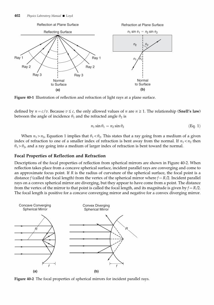
defined by n¼ c/v. Because v £ c, the only allowed values of n are n ‡ 1. The relationship (Snell’s law)between the angle of incidence y1 and the refracted angle y2 is
n1 sin y1 ¼ n2 sin y2 ðEq: 1Þ
When n1 >n2, Equation 1 implies that y1 < y2. This states that a ray going from a medium of a givenindex of refraction to one of a smaller index of refraction is bent away from the normal. If n1 < n2 theny1 > y2, and a ray going into a medium of larger index of refraction is bent toward the normal.
Focal Properties of Reflection and Refraction
Descriptions of the focal properties of reflection from spherical mirrors are shown in Figure 40-2. Whenreflection takes place from a concave spherical surface, incident parallel rays are converging and come toan approximate focus point. If R is the radius of curvature of the spherical surface, the focal point is adistance f (called the focal length) from the vertex of the spherical mirror where f¼R/2. Incident parallelrays on a convex spherical mirror are diverging, but they appear to have come from a point. The distancefrom the vertex of the mirror to that point is called the focal length, and its magnitude is given by f¼R/2.The focal length is positive for a concave converging mirror and negative for a convex diverging mirror.
Reflection at Plane Surface Refraction at Plane Surface
n1 sin �1 � n2 sin �2
Ray 1 Ray 1
Ray 3 Ray 3
Normalto Surface
Normalto Surface
Ray 2 Ray 2
Reflecting Surface
n2 �2
n1 �1
(a) (b)
Figure 40-1 Illustration of reflection and refraction of light rays at a plane surface.
f
R
f
R
Concave ConvergingSpherical Mirror
Convex DivergingSpherical Mirror
(a) (b)
Figure 40-2 The focal properties of spherical mirrors for incident parallel rays.
402 Physics Laboratory Manual n Loyd
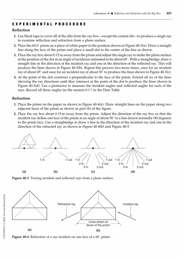
E X P E R I M E N T A L P R O C E D U R EReflection
1. Use black tape to cover all of the slits from the ray box—except the central slit—to produce a single rayto examine reflection and refraction from a plane surface.
2. Place the 60.08 prism on a piece of white paper in the position shown in Figure 40-3(a). Draw a straightline along the face of the prism and place a small dot in the center of the line as shown.
3. Place the ray box about 0.15m away from the prism and adjust the single ray to strike the plane surfaceat the position of the dot at an angle of incidence estimated to be about 608. With a straightedge, draw astraight line in the direction of the incident ray and one in the direction of the reflected ray. This willproduce the lines shown in Figure 40-3(b). Repeat this process two more times, once for an incidentray of about 458 and once for an incident ray of about 308 to produce the lines shown in Figure 40-3(c).
4. At the point of the dot construct a perpendicular to the face of the prism. Extend all six of the linesshowing the ray directions until they intersect at the point of the dot to produce the lines shown inFigure 40-3(d). Use a protractor to measure the incident angles and reflected angles for each of therays. Record all these angles (to the nearest 0.18) in the Data Table.
Refraction
1. Place the prism on the paper as shown in Figure 40-4(a). Draw straight lines on the paper along twoadjacent faces of the prism as shown in part (b) of the figure.
2. Place the ray box about 0.15m away from the prism. Adjust the direction of the ray box so that theincident ray strikes one face of the prism at an angle of about 508 to a line drawn normally (90 degrees)to the prism face. Use a straightedge to draw a line in the direction of the incident ray and one in thedirection of the refracted ray as shown in Figure 40-4(b) and Figure 40-5.
COPYRIG
HTª
2008ThomsonBrooks/Cole
(a)
1 in 1 out 1 in2 in
3 in
1 in2 in
3 in3 out2 out
1 out
3 out2 out
1 out
(b) (c) (d)
Figure 40-3 Tracing incident and reflected rays from a plane surface.
Refracted ray Incident ray
Lines drawn atfaces of the prism
(b)(a)
Figure 40-4 Refraction of a ray incident on one face of a 608 prism.
Laboratory 40 n Reflection and Refraction with the Ray Box 403
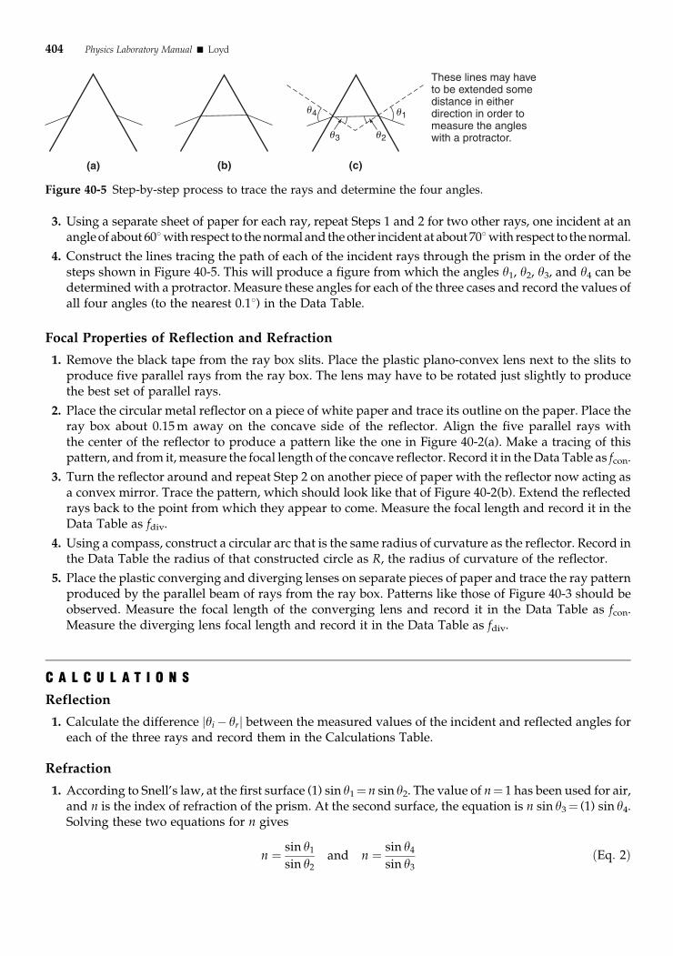
3. Using a separate sheet of paper for each ray, repeat Steps 1 and 2 for two other rays, one incident at anangleof about 608with respect to thenormal and theother incident at about 708with respect to thenormal.
4. Construct the lines tracing the path of each of the incident rays through the prism in the order of thesteps shown in Figure 40-5. This will produce a figure from which the angles y1, y2, y3, and y4 can bedeterminedwith a protractor. Measure these angles for each of the three cases and record the values ofall four angles (to the nearest 0.18) in the Data Table.
Focal Properties of Reflection and Refraction
1. Remove the black tape from the ray box slits. Place the plastic plano-convex lens next to the slits toproduce five parallel rays from the ray box. The lens may have to be rotated just slightly to producethe best set of parallel rays.
2. Place the circular metal reflector on a piece of white paper and trace its outline on the paper. Place theray box about 0.15m away on the concave side of the reflector. Align the five parallel rays withthe center of the reflector to produce a pattern like the one in Figure 40-2(a). Make a tracing of thispattern, and from it, measure the focal length of the concave reflector. Record it in theData Table as fcon.
3. Turn the reflector around and repeat Step 2 on another piece of paper with the reflector now acting asa convex mirror. Trace the pattern, which should look like that of Figure 40-2(b). Extend the reflectedrays back to the point from which they appear to come. Measure the focal length and record it in theData Table as fdiv.
4. Using a compass, construct a circular arc that is the same radius of curvature as the reflector. Record inthe Data Table the radius of that constructed circle as R, the radius of curvature of the reflector.
5. Place the plastic converging and diverging lenses on separate pieces of paper and trace the ray patternproduced by the parallel beam of rays from the ray box. Patterns like those of Figure 40-3 should beobserved. Measure the focal length of the converging lens and record it in the Data Table as fcon.Measure the diverging lens focal length and record it in the Data Table as fdiv.
C A L C U L A T I O N SReflection
1. Calculate the difference jyi � yrj between the measured values of the incident and reflected angles foreach of the three rays and record them in the Calculations Table.
Refraction
1. According to Snell’s law, at the first surface (1) sin y1¼ n sin y2. The value of n¼ 1 has been used for air,and n is the index of refraction of the prism. At the second surface, the equation is n sin y3¼ (1) sin y4.Solving these two equations for n gives
n ¼ sin y1sin y2
and n ¼ sin y4sin y3
ðEq: 2Þ
These lines may haveto be extended somedistance in eitherdirection in order tomeasure the angleswith a protractor.
(a) (b) (c)
�4
�2�3
�1
Figure 40-5 Step-by-step process to trace the rays and determine the four angles.
404 Physics Laboratory Manual n Loyd
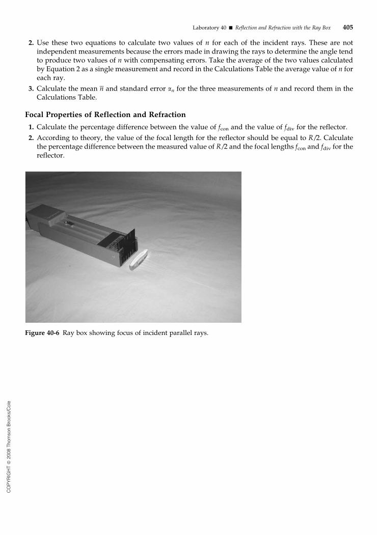
2. Use these two equations to calculate two values of n for each of the incident rays. These are notindependent measurements because the errors made in drawing the rays to determine the angle tendto produce two values of n with compensating errors. Take the average of the two values calculatedby Equation 2 as a single measurement and record in the Calculations Table the average value of n foreach ray.
3. Calculate the mean n and standard error an for the three measurements of n and record them in theCalculations Table.
Focal Properties of Reflection and Refraction
1. Calculate the percentage difference between the value of fcon and the value of fdiv for the reflector.
2. According to theory, the value of the focal length for the reflector should be equal to R/2. Calculatethe percentage difference between the measured value of R/2 and the focal lengths fcon and fdiv for thereflector.
COPYRIG
HTª
2008ThomsonBrooks/Cole
Figure 40-6 Ray box showing focus of incident parallel rays.
Laboratory 40 n Reflection and Refraction with the Ray Box 405

This page intentionally left blank
Name . . . . . . . . . . . . . . . . . . . . . . . . . . . . . . . . . . . . . . . . . . . . . . . . . . . . . . . . . . . . . . . . . . . . . . . . . Section . . . . . . . . . . . . . . . . Date . . . . . . . . . . . . . . . .
40 L A B O R A T O R Y 4 0 Reflection and Refraction with the Ray Box
P R E - L A B O R A T O R Y A S S I G N M E N T1. Define the index of refraction.
2. State the law of reflection. Use a diagram to define the angles involved.
3. State Snell’s law. Define terms and angles using a diagram.
4. A light ray is incident on a plane interface between two media. The ray makes an incident angle withthe normal of 25.08 in a medium of n¼ 1.25. What is the angle that the refracted ray makes with thenormal if the second medium has n¼ 1.55? Show your work.
COPYRIG
HTª
2008ThomsonBrooks/Cole
407

5. A 60.08 prism has an index of refraction of 1.45 as shown below. A ray is incident as shown at an angleof 60.08 to the normal of one of the prism faces. Trace the ray on through the prism and find the anglesy2, y3, and y4 as defined in the laboratory instructions. Show your work.
n � 1.0060°
60°
n � 1.00
n � 1.45
408 Physics Laboratory Manual n Loyd

Name . . . . . . . . . . . . . . . . . . . . . . . . . . . . . . . . . . . . . . . . . . . . . . . . . . . . . . . . . . . . . . . . . . . . . . . . . Section . . . . . . . . . . . . . . . . Date . . . . . . . . . . . . . . . .
Lab Partners . . . . . . . . . . . . . . . . . . . . . . . . . . . . . . . . . . . . . . . . . . . . . . . . . . . . . . . . . . . . . . . . . . . . . . . . . . . . . . . . . . . . . . . . . . . . . . . . . . . . . . . . . . . . . . . . . . . .
40 L A B O R A T O R Y 4 0 Reflection and Refraction with the Ray Box
L A B O R A T O R Y R E P O R T
COPYRIG
HTª
2008ThomsonBrooks/Cole
Data Table
Reflection
Ray yi yr
Calculations Table
Angle Difference
Refraction
Ray y1 y2 y3 y4 n n an
Mirrors
f (cm) R (cm)
Concave fcon
Convex fdiv
% Diff of f % Diff of R/2
Lenses
f (cm)
Converging Lens
Diverging Lens
409
S A M P L E C A L C U L A T I O N S1. Angle Difference¼ jyi � yrj ¼2. n ¼ ½
sin y1sin y2
þ sin y4sin y3
� ¼
3. % Diff between fcon and fdiv¼4. % Diff between f and R/2¼
Q U E S T I O N S1. Are your data consistent with the law of reflection? State your answer as quantitatively as possible.
2. State as quantitatively as possible the precision of your value for n, the index of refraction of the prism.
3. State how your data for the prism are evidence for the validity of Snell’s law.
4. How well do your data for the focal lengths of the concave and convex mirror agree with theexpectation that f¼R/2? State your answer as quantitatively as possible.
5. Using the value of n determined for the prism, find the speed of light in the prism.
410 Physics Laboratory Manual n Loyd

6. Inside the prism the wavelength of the light must change as well as the speed. Is a given wavelengthlonger or shorter inside the prism? Consider specifically light with a wavelength of 500 nm in air.What is the wavelength of this light inside the prism?
COPYRIG
HTª
2008ThomsonBrooks/Cole
Laboratory 40 n Reflection and Refraction with the Ray Box 411

This page intentionally left blank

Focal Length of Lenses
O B J E C T I V E So Investigate the properties of converging and diverging lenses.
o Determine the focal length of converging lenses both by a real image of a distant object and byfinite object and image distances.
o Determine the focal length of a diverging lens by using it in combination with a converging lensto form a real image.
E Q U I P M E N T L I S T. Optical bench, holders for lenses, a screen to form images, meter stick, tape
. Lamp with object on face (illuminated object), three lenses (f�þ20,þ10,�30 cm)
T H E O R YWhen a beam of light rays parallel to the central axis of a lens is incident upon a converging lens,the rays are brought together at a point called the focal point of the lens. The distance from the centerof the lens to the focal point is called f the focal length of the lens, and it is a positive quantity for aconverging lens. When a parallel beam of light rays is incident upon a diverging lens the rays divergeas they leave the lens; however, if the paths of the outgoing rays are traced backward, the rays appearto have emerged from a point called the focal point of the lens. The distance from the center of thelens to the focal point is called the focal length f of the lens, and it is a negative quantity for a diverginglens. In Figure 41-1 two common types of lenses are pictured. In general, a lens is converging ordiverging depending upon the curvature of its surfaces. In Figure 41-1 the radii of curvature of thesurfaces of the two lenses are denoted as R1 and R2. The relationship that determines the focal length f interms of the radii of curvature and the index of refraction n of the glass of the lens is called the lensmakers equation. It is
1
f¼ ðn� 1Þ 1
R1� 1
R2
� ðEq: 1Þ
For the converging lens shown in Figure 41-1(a) the radius R1 is positive and the radius R2 is negative, butfor the diverging lens of part (b), the radius R1 is negative and the radius R2 is positive. The signs of theseradii are determined according to a sign convention that is described in all elementary textbooks.
Physics Laboratory Manual n Loyd L A B O R A T O R Y 41
COPYRIG
HTª
2008ThomsonBrooks/Cole
413
ª 2008 Thomson Brooks/Cole, a part of TheThomson Corporation.Thomson, the Star logo, and Brooks/Cole are trademarks used herein under license. ALL RIGHTSRESERVED.No part of this workcovered by the copyright hereonmay be reproduced or used in any form or by any meansçgraphic, electronic, ormechanical, including photocopying, recording, taping,web distribution, informationstorage and retrieval systems,or in any othermannerçwithout the written permission of the publisher.
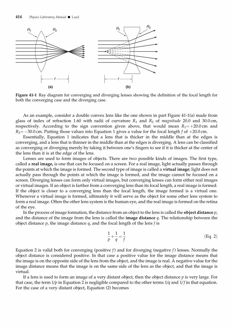
As an example, consider a double convex lens like the one shown in part Figure 41-1(a) made fromglass of index of refraction 1.60 with radii of curvature R1 and R2 of magnitude 20.0 and 30.0 cm,respectively. According to the sign convention given above, that would mean R1¼þ20.0 cm andR2¼�30.0 cm. Putting those values into Equation 1 gives a value for the focal length f of þ20.0 cm.
Essentially, Equation 1 indicates that a lens that is thicker in the middle than at the edges isconverging, and a lens that is thinner in the middle than at the edges is diverging. A lens can be classifiedas converging or diverging merely by taking it between one’s fingers to see if it is thicker at the center ofthe lens than it is at the edge of the lens.
Lenses are used to form images of objects. There are two possible kinds of images. The first type,called a real image, is one that can be focused on a screen. For a real image, light actually passes throughthe points at which the image is formed. The second type of image is called a virtual image; light does notactually pass through the points at which the image is formed, and the image cannot be focused on ascreen. Diverging lenses can form only virtual images, but converging lenses can form either real imagesor virtual images. If an object is farther from a converging lens than its focal length, a real image is formed.If the object is closer to a converging lens than the focal length, the image formed is a virtual one.Whenever a virtual image is formed, ultimately it will serve as the object for some other lens system toform a real image. Often the other lens system is the human eye, and the real image is formed on the retinaof the eye.
In the process of image formation, the distance from an object to the lens is called the object distance p,and the distance of the image from the lens is called the image distance q. The relationship between theobject distance p, the image distance q, and the focal length of the lens f is
1
pþ 1
q¼ 1
fðEq: 2Þ
Equation 2 is valid both for converging (positive f ) and for diverging (negative f ) lenses. Normally theobject distance is considered positive. In that case a positive value for the image distance means thatthe image is on the opposite side of the lens from the object, and the image is real. A negative value for theimage distance means that the image is on the same side of the lens as the object, and that the image isvirtual.
If a lens is used to form an image of a very distant object, then the object distance p is very large. Forthat case, the term 1/p in Equation 2 is negligible compared to the other terms 1/q and 1/f in that equation.For the case of a very distant object, Equation (2) becomes
(a)
R1 R2
(b)
f
R1R2
f
Figure 41-1 Ray diagram for converging and diverging lenses showing the definition of the focal length forboth the converging case and the diverging case.
414 Physics Laboratory Manual n Loyd

1
q¼ 1
fðEq: 3Þ
For this case, the image distance is equal to the focal length. This provides a quick and accurate way todetermine the focal length of a converging lens, but it is only applicable to a converging lens because theimage must be focused on a screen. A diverging lens cannot form a real image, and this technique will notwork directly for a diverging lens.
If two lenses with focal lengths of f1 and f2 are placed in contact, the combination of the two in contactacts as a single lens of effective focal length fe. The effective focal length of the two lenses in contact fe isrelated to the individual focal lengths of the lenses f1 and f2 by
1
fe¼ 1
f1þ 1
f2ðEq: 4Þ
Equation 4 is valid for any combination of converging and diverging lenses. If the individual lenses f1 and f2are converging, then the effective focal length fe will also be converging. If one of the lenses is convergingand the other is diverging, then the effective focal length can be either converging or diverging dependingupon the values of f1 and f2. If the converging lens has a smaller magnitude than the diverging lens, thenthe effective focal length will be converging. We can use this fact to determine the focal length of anunknown diverging lens if it is used in combination with a converging lens with a focal length shortenough to produce a converging combination.
E X P E R I M E N T A L P R O C E D U R EFocal Length of a Single Lens
1. Place one of the three lenses in a lens holder on the optical bench and place the screen in its holder onthe optical bench. Place the optical bench in front of a window in the laboratory and point the benchtoward some distant object. Adjust the distance from the lens to the screen until a sharp, real imageof the distant object is formed on the screen. You will be able to form such an image for only two ofthe three lenses. This experimental arrangement satisfies the conditions of Equation 3. The measuredimage distance is equal to the focal length of the lens. Record these measured image distances in DataTable 1 as the focal length of the two lenses for which the method works. Call the lens with the longestfocal lengthA, the onewith the shortest focal length B, and the one forwhich no image can be formedC.
2. Place lens B in the lens holder on the optical bench and use the lampwith the object painted on its faceas an object. For various distances p of the object from the lens, move the screen until a sharp realimage is formed on the screen. For each value of pmeasure the image distance q from the screen to the
COPYRIG
HTª
2008ThomsonBrooks/Cole
Figure 41-2 Optical bench with object, lens, and screen on which a real image is formed.
Laboratory 41 n Focal Length of Lenses 415
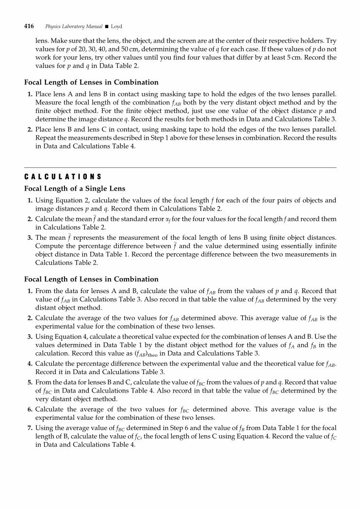
lens. Make sure that the lens, the object, and the screen are at the center of their respective holders. Tryvalues for p of 20, 30, 40, and 50 cm, determining the value of q for each case. If these values of p do notwork for your lens, try other values until you find four values that differ by at least 5 cm. Record thevalues for p and q in Data Table 2.
Focal Length of Lenses in Combination
1. Place lens A and lens B in contact using masking tape to hold the edges of the two lenses parallel.Measure the focal length of the combination fAB both by the very distant object method and by thefinite object method. For the finite object method, just use one value of the object distance p anddetermine the image distance q. Record the results for both methods in Data and Calculations Table 3.
2. Place lens B and lens C in contact, using masking tape to hold the edges of the two lenses parallel.Repeat the measurements described in Step 1 above for these lenses in combination. Record the resultsin Data and Calculations Table 4.
C A L C U L A T I O N SFocal Length of a Single Lens
1. Using Equation 2, calculate the values of the focal length f for each of the four pairs of objects andimage distances p and q. Record them in Calculations Table 2.
2. Calculate the mean f and the standard error af for the four values for the focal length f and record themin Calculations Table 2.
3. The mean f represents the measurement of the focal length of lens B using finite object distances.Compute the percentage difference between f and the value determined using essentially infiniteobject distance in Data Table 1. Record the percentage difference between the two measurements inCalculations Table 2.
Focal Length of Lenses in Combination
1. From the data for lenses A and B, calculate the value of fAB from the values of p and q. Record thatvalue of fAB in Calculations Table 3. Also record in that table the value of fAB determined by the verydistant object method.
2. Calculate the average of the two values for fAB determined above. This average value of fAB is theexperimental value for the combination of these two lenses.
3. Using Equation 4, calculate a theoretical value expected for the combination of lenses A and B. Use thevalues determined in Data Table 1 by the distant object method for the values of fA and fB in thecalculation. Record this value as (fAB)theo in Data and Calculations Table 3.
4. Calculate the percentage difference between the experimental value and the theoretical value for fAB.Record it in Data and Calculations Table 3.
5. From the data for lenses B and C, calculate the value of fBC from the values of p and q. Record that valueof fBC in Data and Calculations Table 4. Also record in that table the value of fBC determined by thevery distant object method.
6. Calculate the average of the two values for fBC determined above. This average value is theexperimental value for the combination of these two lenses.
7. Using the average value of fBC determined in Step 6 and the value of fB from Data Table 1 for the focallength of B, calculate the value of fC, the focal length of lens C using Equation 4. Record the value of fCin Data and Calculations Table 4.
416 Physics Laboratory Manual n Loyd
Name . . . . . . . . . . . . . . . . . . . . . . . . . . . . . . . . . . . . . . . . . . . . . . . . . . . . . . . . . . . . . . . . . . . . . . . . . Section . . . . . . . . . . . . . . . . Date . . . . . . . . . . . . . . . .
41 L A B O R A T O R Y 4 1 Focal Length of Lenses
P R E - L A B O R A T O R Y A S S I G N M E N T1. Mark the following statements about lenses as true or false.
_____a. Incident parallel light rays converge if the lens’s focal length is negative.
_____b. If the path of converging light rays is traced backward, the rays appear to come from a pointcalled the focal point.
_____c. A double convex lens has a negative focal length.
_____d. The focal length of a lens is always positive.
2. A double convex lens is made from glass with an index of refraction of n¼ 1.50. The magnitudes of itsradii of curvature R1 and R2 are 10.0 cm and 15.0 cm, respectively. What is the focal length of the lens?Show your work.
f ¼ cm
3. What is a real image? What is a virtual image?
4. For a diverging lens, state what kinds of images can be formed and the conditions under which thoseimages can be formed.
COPYRIG
HTª
2008ThomsonBrooks/Cole
417

5. For a converging lens, state what kinds of images can be formed and the conditions under which thoseimages can be formed.
6. A lens has a focal length of f¼þ10.0 cm. If an object is placed 30.0 cm from the lens, where is theimage formed? Is the image real or virtual? Show your work.
7. An object is 16.0 cm from a lens. A real image is formed 24.0 cm from the lens. What is the focal lengthof the lens? Show your work.
8. One lens has a focal length of þ15.0 cm. A second lens of focal length þ20.0 cm is placed in contactwith the first lens. What is the equivalent focal length of the combination of lenses? Show your work.
9. Two lenses are in contact. One of the lenses has a focal length of þ10.0 cm when used alone. When thetwo are in combination, an object 20.0 cm away from the lenses forms a real image 40.0 cm away fromthe lenses. What is the focal length of the second lens? Show your work.
418 Physics Laboratory Manual n Loyd

Name . . . . . . . . . . . . . . . . . . . . . . . . . . . . . . . . . . . . . . . . . . . . . . . . . . . . . . . . . . . . . . . . . . . . . . . . . Section . . . . . . . . . . . . . . . . Date . . . . . . . . . . . . . . . .
Lab Partners . . . . . . . . . . . . . . . . . . . . . . . . . . . . . . . . . . . . . . . . . . . . . . . . . . . . . . . . . . . . . . . . . . . . . . . . . . . . . . . . . . . . . . . . . . . . . . . . . . . . . . . . . . . . . . . . . . . .
41 L A B O R A T O R Y 4 1 Focal Length of Lenses
L A B O R A T O R Y R E P O R T
Data Table 1
Lens Image Distance (cm) Focal Length (cm)
A fA¼
B fB¼
Data Table 2
p (cm) q (cm)
Calculations Table 2
fB (cm) fB (cm) af (cm) % Diff
Data and Calculations Table 3 (Lenses A & B)
q (p¼1) p q fAB p¼1 fAB p & q fAB fAB theo % Diff
Data and Calculations Table 4 (Lenses B & C)
q (p¼1) p q fBC p¼1 fBC p & q fBC fC
COPYRIG
HTª
2008ThomsonBrooks/Cole
419

S A M P L E C A L C U L A T I O N S1. f ¼ pq
pþ q¼
2. fAB ¼ ðfAB1 þ fAB2Þ=2 ¼3. (fAB)theo¼ (fA) (fB)/(fAþ fB)¼4. fC¼ (fB)(fBC)/(fB� fBC)¼
Q U E S T I O N S1. Why is it not possible to form a real image with lens C alone?
2. Take lens C between your thumb and index finger. Is it thinner or thicker at the center of the lens thanat the edge? Take lens B between your thumb and index finger. Is it thinner or thicker at the center ofthe lens than at the edge? From this information alone, what can you conclude about lenses C and B?
3. Consider the percentage difference between the two measurements of the focal length of lens B.Express af as a percentage of f : Is the percentage difference between the two measurements less thanthe percentage standard error?
4. Compare the agreement between the experimental and theoretical values of fAB the focal length oflenses A and B combined. Do these data suggest that Equation 4 is a valid model for the equivalentfocal length of two lenses in contact?
5. If lens A and lens C were used in contact, could they produce a real image? State clearly the basis foryour answer. You will need to do a calculation.
420 Physics Laboratory Manual n Loyd
Diffraction Grating Measurementof the Wavelength of Light
O B J E C T I V E So Investigate the difference between continuous and discrete spectra.
o Investigate the characteristic spectra of individual gaseous elements.
o Determine the average line spacing for a diffraction grating assuming mercury wavelengths asknown, and use it to determine the wavelengths of helium.
E Q U I P M E N T L I S T. Optical bench, diffraction grating (600 lines/mm replica grating)
. Spectrum tube power supply, mercury and helium discharge tubes
. Meter stick and slit arrangement, incandescent lightbulb (15 watt)
T H E O R YWhen light is separated into its componentwavelengths, the resulting array of colors is called a spectrum.If a light source produces all the colors of visible light, it is called a continuous spectrum. Generally, suchsources of light are produced by heated solid metal filaments. An ordinary incandescent lightbulb witha tungsten filament produces a continuous spectrum.
Some light sources produce discrete wavelengths of light, and the spectrum appears as mostly darkwith a few discrete lines of color at the wavelengths emitted by the source. Such light is produced by hotdischarges of gas of a single chemical element, and the wavelengths of light emitted are characteristicof the electronic structure of that element. The spectrum is called a discrete spectrum or a line spectrum.The term line spectrum is used because the images produced usually are images of a narrow slit that isilluminated by the light source.
We can use severalmethods to separate light into its componentwavelengths and produce a spectrum.This laboratory will use a diffraction grating to produce spectra from an incandescent lightbulb and fromgas discharge tubes of mercury and helium. A transmission diffraction grating is a piece of transparentmaterial ruledwith a large number of equally spaced parallel lines. The distance between the lines is calledthe grating spacing d, and it is usually only a few times as large as a typical wavelength of visible light.The range of visible light wavelengths is from approximately 4� 10�7m to 7� 10�7m. It is customary toexpress the wavelength of light in units of nm (10�9 m). In those units the range of visible light is from400nm to 700 nm. A typical grating spacing d is in the range 1000 nm to 2000 nm.
Physics Laboratory Manual n Loyd L A B O R A T O R Y 42
COPYRIG
HTª
2008ThomsonBrooks/Cole
421
ª 2008 Thomson Brooks/Cole, a part of TheThomson Corporation.Thomson, the Star logo, and Brooks/Cole are trademarks used herein under license. ALL RIGHTSRESERVED.No part of this workcovered by the copyright hereonmay be reproduced or used in any form or by any meansçgraphic, electronic, ormechanical, including photocopying, recording, taping,web distribution, informationstorage and retrieval systems,or in any othermannerçwithout the written permission of the publisher.

The wavelengths of light determine the color of the light seen by the human eye. Starting from shortwavelengths and going to long wavelengths, the order of colors is violet, blue, green, yellow, orange, andred. The actual range of the visible spectrum is somewhat different for individuals, and there may be adistinct difference in the ability of two laboratory partners to see the wavelengths at either end of thespectrum. It is often very difficult for some people to see the very short wavelengths.
Light rays that strike the transparent portion of the grating between the ruled lines will pass throughthe grating at all angles with respect to their original path. When deviated rays from adjacent rulings onthe grating are in phase, an image of the source will be formed. This condition is satisfied when theadjacent rays differ in path length by an integral number of wavelengths of the light. Thus for a givenwavelength l a series of images will appear at angles ym that satisfy the equation
m l ¼ d sin ym ðEq: 1Þ
withm an integer. The first value of y is y1 whenm¼ 1, the second is y2 whenm¼ 2. Figure 42-1 shows thatthe limit to the values of ywill be at y¼ 908. This is referred to as the number of orders that can be seen andis determined by d and l. Although it will be possible to see both first-order (m¼ 1) and second-order(m¼ 2) for the experimental arrangement used in this laboratory, measurements will be made only on thefirst-order images.
The experimental arrangement is shown in Figure 42-2. The discharge tube light source is viewedthrough the grating as shown. The distance L from the grating to the slit is chosen at a convenient fixed
d
d sin�1
�1
d
d
Figure 42-1 Ray diagram for the conditions of the first-order diffraction image.
Grating
Eye
Optical Bench
Meter Stick
Slit
LightSource
Image
D
�
L
Figure 42-2 Arrangement of the diffraction grating, slit, light source, and optical bench.
422 Physics Laboratory Manual n Loyd
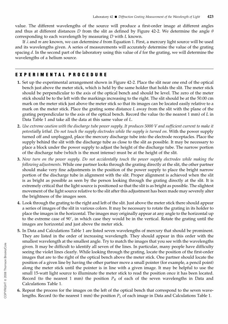
value. The different wavelengths of the source will produce a first-order image at different anglesand thus at different distances D from the slit as defined by Figure 42-2. We determine the angle ycorresponding to each wavelength by measuring D with L known.
If l and m are known, we can determine d from Equation 1. First, a mercury light source will be usedand its wavelengths given. A series of measurements will accurately determine the value of the gratingspacing d. In the second part of the laboratory using this value of d for the grating, we will determine thewavelengths of a helium source.
E X P E R I M E N T A L P R O C E D U R E1. Set up the experimental arrangement shown in Figure 42-2. Place the slit near one end of the optical
bench just above the meter stick, which is held by the same holder that holds the slit. The meter stickshould be perpendicular to the axis of the optical bench and should be level. The zero of the meterstick should be to the left with the markings increasing to the right. The slit should be at the 50.00 cmmark on the meter stick just above the meter stick so that its images can be located easily relative to amark on the meter stick. Place the grating some distance L away from the slit with the plane of thegrating perpendicular to the axis of the optical bench. Record the value (to the nearest 1 mm) of L inData Table 1 and take all the data at this same value of L.
2. Use extreme caution with the discharge tube power supply. It produces 5000 V and sufficient current to make itpotentially lethal. Do not touch the supply electrodes while the supply is turned on. With the power supplyturned off and unplugged, place the mercury discharge tube into the electrode receptacles. Place thesupply behind the slit with the discharge tube as close to the slit as possible. It may be necessary toplace a block under the power supply to adjust the height of the discharge tube. The narrow portionof the discharge tube (which is the most intense) must be at the height of the slit.
3. Now turn on the power supply. Do not accidentally touch the power supply electrodes while making thefollowing adjustments. While one partner looks through the grating directly at the slit, the other partnershould make very fine adjustments in the position of the power supply to place the bright narrowportion of the discharge tube in alignment with the slit. Proper alignment is achieved when the slitis as bright as possible as seen by the person looking through the grating directly at the slit. It isextremely critical that the light source is positioned so that the slit is as bright as possible. The slightestmovement of the light source relative to the slit after this adjustment has beenmademay severely alterthe brightness of the images seen.
4. Look through the grating to the right and left of the slit. Just above the meter stick there should appeara series of images of the slit in various colors. It may be necessary to rotate the grating in its holder toplace the images in the horizontal. The images may originally appear at any angle to the horizontal upto the extreme case of 908, in which case they would be in the vertical. Rotate the grating until theimages are horizontal and just above the meter stick.
5. In Data and Calculations Table 1 are listed seven wavelengths of mercury that should be prominent.They are listed in the order of increasing wavelength. They should appear in this order with thesmallest wavelength at the smallest angle. Try to match the images that you see with the wavelengthsgiven. It may be difficult to identify all seven of the lines. In particular, many people have difficultyseeing the violet lines clearly. While looking through the grating, locate the position of the first-orderimages that are to the right of the optical bench above the meter stick. One partner should locate theposition of a given line by having the other partner move a small pointer (for example, a pencil point)along the meter stick until the pointer is in line with a given image. It may be helpful to use thesmall 15-watt light source to illuminate the meter stick to read the position once it has been located.Record (to the nearest 1 mm) the position PR of each of the seven wavelengths in Data andCalculations Table 1.
6. Repeat the process for the images on the left of the optical bench that correspond to the seven wave-lengths. Record (to the nearest 1 mm) the position PL of each image in Data and Calculations Table 1.
COPYRIG
HTª
2008ThomsonBrooks/Cole
Laboratory 42 n Diffraction Grating Measurement of the Wavelength of Light 423

7. Turn off the power supply and allow the discharge tube to cool. With the power supply turned off,remove the mercury discharge tube and replace it with the helium discharge tube. Position the powersupply with the discharge tube alignedwith the slit. Turn on the power supply and adjust the positionof the supply for maximum brightness.
8. In Data and Calculations Table 2 are listed eight wavelengths of helium that should be visible. Againtry to match the images that you see with the wavelengths given. Perform the same procedure as doneabove for mercury, measuring the positions PR and PL of each image on the right and the left. Record(to the nearest 1 mm) the data in Data and Calculations Table 2.
9. Place the 15-watt lightbulb behind the slit and observe the continuous spectrum. Locate the positionsPR and PL of the following parts of the spectrum: (a) the shortest wavelength visible (b) the divisionbetween blue and green (c) the division between green and yellow (d) the division between yellowand orange (e) the division between orange and red (f ) the longest wavelength visible. Record (to thenearest 1 mm) the position of these points in Data and Calculations Table 3.
C A L C U L A T I O N S1. Calculate the distance DR from the slit to each image on the right (DR¼PR� 50.0) and calculate the
distanceDL from the slit to each image on the left (DL¼ 50.0�PL) for the mercury data in Data Table 1.Calculate the average distanceD ¼ ðDR þDLÞ=2 and calculate tan y ¼ D=L, y, and sin y for each image.Record (to three significant figures) those values in Data and Calculations Table 1.
2. Each of the measurements for mercury is an independent measurement for d the grating spacing.Use Equation 1 to calculate the seven values of d, and record them (to four significant figures) in Dataand Calculations Table 1. Calculate the mean d and the standard error ad for d and record them inData and Calculations Table 1.
3. Calculate the values ofDR,DL, andD for the helium data and use them to calculate tan y ¼ D=L, y, andsin y for each image. Use those values of sin y and d in Equation 1 to calculate the wavelengths ofhelium. Record all values (to three significant figures) in Data and Calculations Table 2.
4. From the data for the continuous spectrum, determine the wavelength that corresponds to the variouspoints in the spectrum that were located. Calculate and record all the information called for in Dataand Calculations Table 3.
424 Physics Laboratory Manual n Loyd
Name . . . . . . . . . . . . . . . . . . . . . . . . . . . . . . . . . . . . . . . . . . . . . . . . . . . . . . . . . . . . . . . . . . . . . . . . . Section . . . . . . . . . . . . . . . . Date . . . . . . . . . . . . . . . .
42 L A B O R A T O R Y 4 2 Diffraction Grating Measurement of the Wavelengthof Light
P R E - L A B O R A T O R Y A S S I G N M E N T1. What is a continuous spectrum? What is a discrete spectrum?
2. What kind of light sources produce each type of spectrum?
3. The wavelengths produced by a hot gas of helium (a) form a discrete spectrum (b) form a linespectrum (c) are characteristic of the electronic structure of helium (d) all of the above are true.
4. A diffraction grating has a grating spacing of d¼ 1500nm. It is used with light of wavelength 500 nm.At what angle will the first-order diffraction image be seen? Show your work.
5. For a given wavelength l and a diffraction grating of spacing d (a) an image is formed at only oneangle (b) at least two orders are always seen (c) the number of orders seen can be any number anddepends on d and l (d) there can never be more than four orders seen.
6. The grating used in this laboratory (a) can produce only images in the horizontal (b) must be rotated inits holder until it produces the desired horizontal pattern (c) produces images only in the verticaldirection (d) produces images only to the left of the slit.
COPYRIG
HTª
2008ThomsonBrooks/Cole
425

7. A diffraction grating with d¼ 2000nm is used with a mercury discharge tube. At what angle will thefirst-order blue-green wavelength of mercury appear? What other orders can be seen, and at whatangle will they appear? Show your work.
8. The diffraction grating of Question 7 is used at a distance L¼ 50.0 cm from the slit. What is the distanceD from the slit to the first-order image for the blue-green wavelength of mercury? Show your work.
9. What is the voltage and current of the spectrum tube power supply?
426 Physics Laboratory Manual n Loyd

Name . . . . . . . . . . . . . . . . . . . . . . . . . . . . . . . . . . . . . . . . . . . . . . . . . . . . . . . . . . . . . . . . . . . . . . . . . Section . . . . . . . . . . . . . . . . Date . . . . . . . . . . . . . . . .
Lab Partners . . . . . . . . . . . . . . . . . . . . . . . . . . . . . . . . . . . . . . . . . . . . . . . . . . . . . . . . . . . . . . . . . . . . . . . . . . . . . . . . . . . . . . . . . . . . . . . . . . . . . . . . . . . . . . . . . . . .
42 L A B O R A T O R Y 4 2 Diffraction Grating Measurement of the Wavelengthof Light
L A B O R A T O R Y R E P O R T
COPYRIG
HTª
2008ThomsonBrooks/Cole
Data and Calculations Table 1 (Mercury Spectrum)
Colors l (nm) PR (cm) PL (cm) DR (cm) DL (cm) D (cm) tan y y sin y d (nm)
Violet 404.7
Violet 407.8
Blue 435.8
Blu-Gr 491.6
Green 546.1
Yellow 577.0
Yellow 579.0
L¼ cm d ¼ nm ad¼ nm
427

S A M P L E C A L C U L A T I O N S1. DR¼PR� 50.0 ¼ and DL¼ 50.0�PL¼2. D ¼ ðDR þDLÞ=2 ¼3. tan y ¼ D=L ¼ and y ¼ tan�1ðyÞ ¼4. sin y ¼5. d¼ l/sin y ¼6. l ¼ d sin y ¼
Data and Calculations Table 2 (Helium Spectrum)
Colors l (nm) PR (cm) PL (cm) DR (cm) DL (cm) D (cm) tan y y sin y l (nm)
Blue 438.8
Blue 447.1
Blue 471.3
Blu-Gr 492.2
Green 501.5
Yellow 587.6
Red 667.8
Red 706.5
Data and Calculations Table 3 (Continuous Spectrum)
Portion of Spectrum PR (cm) PL (cm) D (cm) tan y y sin y l (nm)
Shortest Wavelength
Division Blue and Green
Division Green and Yellow
Division Yellow and Orange
Division Orange and Red
Longest Wavelength
428 Physics Laboratory Manual n Loyd
Q U E S T I O N S1. Comment on the precision of your measurement of d.
2. List the accepted values of the eight wavelengths of helium below. Beside each one, show thepercentage error in your measured values compared to these values including the sign of the error.Comment on the accuracy of your measurements.
3. If all the errors in Question 2 are of the same sign, it might be evidence of a systematic error. Based onthis criterion, do your data show evidence of a systematic error? State your evidence for or against asystematic error.
4. If the grating had exactly 600 lines/mm, d would be 1667nm. Use that value of d with the values ofsin y in Table 2 to recalculate the wavelengths for helium. Are their percentage differences from theaccepted values better or worse than in Question 2? Show your work.
5. Hydrogen has known emission lines of wavelength 656.3 nm and 434.1 nm. At what distance D awayfrom the slitwould each of these lines be observed in your experimental arrangement? Showyourwork.
COPYRIG
HTª
2008ThomsonBrooks/Cole
Laboratory 42 n Diffraction Grating Measurement of the Wavelength of Light 429

This page intentionally left blank

Bohr Theory of Hydrogen—The Rydberg Constant
O B J E C T I V E So Investigate how well the visible light wavelengths of hydrogen predicted by the Bohr theory
agree with experimental values.
o Determine an experimental value for the Rydberg constant from a fit of the measured values ofhydrogen wavelengths to the form of the Balmer equation.
E Q U I P M E N T L I S T. Spectrometer, diffraction grating in holder (600 lines/mm or better)
. Hydrogen gas discharge tube, mercury discharge tube
. Power supply for the discharge tubes
T H E O R YThe spectrum from a hot gas of an element consists of discrete wavelengths that are characteristic of theelement. In 1885, in an attempt to understand these spectra, Johann Balmer published an empiricalrelationship that described the visible spectrum of hydrogen. Although Balmer published the relationshipin a somewhat different form, the modern equivalent is
1
l¼ RH
1
22� 1
n2
� n ¼ 3; 4; 5; 6::::: ðEq: 1Þ
where RH¼ 1.097� 107 m�1 is a constant called the Rydberg constant, l stands for the wavelength, and nis an integer that takes on successive values greater than 2. In 1913 Neils Bohr was able to derive theBalmer relationship by making a series of revolutionary postulates. The Bohr theory was historically ofgreat importance in the developments that eventually led to modern quantum theory. In his attempts toexplain the spectrum of hydrogen, Bohr was influenced by several recently developed theories. Heincorporated concepts from the quantum theory of Max Planck, from the photon description of light byAlbert Einstein, and from the nuclear theory of the atom suggested by Ernest Rutherford’s a-particle
Physics Laboratory Manual n Loyd L A B O R A T O R Y 43
COPYRIG
HTª
2008ThomsonBrooks/Cole
431
ª 2008 Thomson Brooks/Cole, a part of TheThomson Corporation.Thomson, the Star logo, and Brooks/Cole are trademarks used herein under license. ALL RIGHTSRESERVED.No part of this workcovered by the copyright hereonmay be reproduced or used in any form or by any meansçgraphic, electronic, ormechanical, including photocopying, recording, taping,web distribution, informationstorage and retrieval systems,or in any othermannerçwithout the written permission of the publisher.
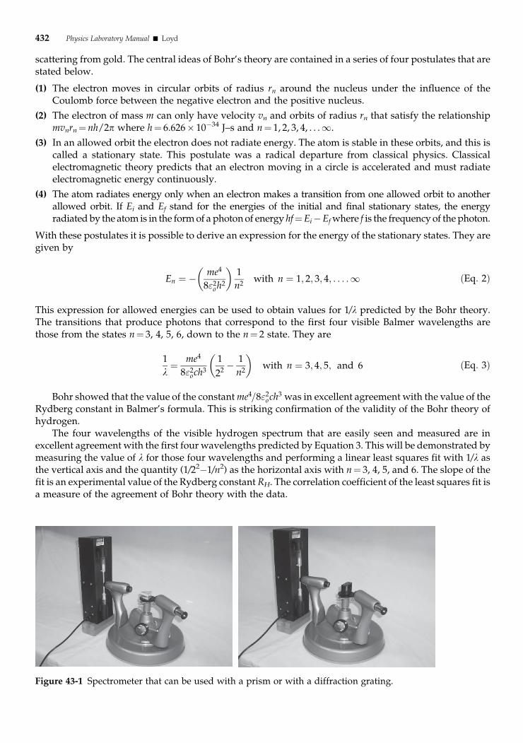
scattering from gold. The central ideas of Bohr’s theory are contained in a series of four postulates that arestated below.
(1) The electron moves in circular orbits of radius rn around the nucleus under the influence of theCoulomb force between the negative electron and the positive nucleus.
(2) The electron of mass m can only have velocity vn and orbits of radius rn that satisfy the relationshipmvnrn¼ nh/2p where h¼ 6.626� 10�34 J–s and n¼ 1, 2, 3, 4, . . .1.
(3) In an allowed orbit the electron does not radiate energy. The atom is stable in these orbits, and this iscalled a stationary state. This postulate was a radical departure from classical physics. Classicalelectromagnetic theory predicts that an electron moving in a circle is accelerated and must radiateelectromagnetic energy continuously.
(4) The atom radiates energy only when an electron makes a transition from one allowed orbit to anotherallowed orbit. If Ei and Ef stand for the energies of the initial and final stationary states, the energyradiated by the atom is in the formof a photonof energy hf¼Ei�Efwhere f is the frequency of the photon.
With these postulates it is possible to derive an expression for the energy of the stationary states. They aregiven by
En ¼ � me4
8"2oh2
� 1
n2with n ¼ 1; 2; 3; 4; : : : :1 ðEq: 2Þ
This expression for allowed energies can be used to obtain values for 1/l predicted by the Bohr theory.The transitions that produce photons that correspond to the first four visible Balmer wavelengths arethose from the states n¼ 3, 4, 5, 6, down to the n¼ 2 state. They are
1
l¼ me4
8"2och3
1
22� 1
n2
� with n ¼ 3; 4; 5; and 6 ðEq: 3Þ
Bohr showed that the value of the constantme4=8"2och3 was in excellent agreement with the value of the
Rydberg constant in Balmer’s formula. This is striking confirmation of the validity of the Bohr theory ofhydrogen.
The four wavelengths of the visible hydrogen spectrum that are easily seen and measured are inexcellent agreement with the first four wavelengths predicted by Equation 3. This will be demonstrated bymeasuring the value of l for those four wavelengths and performing a linear least squares fit with 1/l asthe vertical axis and the quantity (1/22�1/n2) as the horizontal axis with n¼ 3, 4, 5, and 6. The slope of thefit is an experimental value of the Rydberg constant RH. The correlation coefficient of the least squares fit isa measure of the agreement of Bohr theory with the data.
Figure 43-1 Spectrometer that can be used with a prism or with a diffraction grating.
432 Physics Laboratory Manual n Loyd
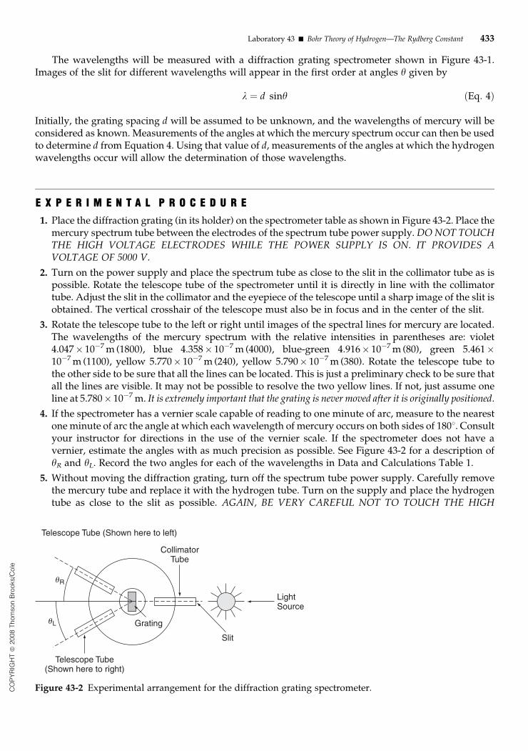
The wavelengths will be measured with a diffraction grating spectrometer shown in Figure 43-1.Images of the slit for different wavelengths will appear in the first order at angles y given by
l ¼ d siny ðEq: 4Þ
Initially, the grating spacing d will be assumed to be unknown, and the wavelengths of mercury will beconsidered as known. Measurements of the angles at which the mercury spectrum occur can then be usedto determine d from Equation 4. Using that value of d, measurements of the angles at which the hydrogenwavelengths occur will allow the determination of those wavelengths.
E X P E R I M E N T A L P R O C E D U R E1. Place the diffraction grating (in its holder) on the spectrometer table as shown in Figure 43-2. Place the
mercury spectrum tube between the electrodes of the spectrum tube power supply.DONOT TOUCHTHE HIGH VOLTAGE ELECTRODES WHILE THE POWER SUPPLY IS ON. IT PROVIDES AVOLTAGE OF 5000 V.
2. Turn on the power supply and place the spectrum tube as close to the slit in the collimator tube as ispossible. Rotate the telescope tube of the spectrometer until it is directly in line with the collimatortube. Adjust the slit in the collimator and the eyepiece of the telescope until a sharp image of the slit isobtained. The vertical crosshair of the telescope must also be in focus and in the center of the slit.
3. Rotate the telescope tube to the left or right until images of the spectral lines for mercury are located.The wavelengths of the mercury spectrum with the relative intensities in parentheses are: violet4.047� 10�7m (1800), blue 4.358� 10�7m (4000), blue-green 4.916� 10�7m (80), green 5.461�10�7m (1100), yellow 5.770� 10�7m (240), yellow 5.790� 10�7m (380). Rotate the telescope tube tothe other side to be sure that all the lines can be located. This is just a preliminary check to be sure thatall the lines are visible. It may not be possible to resolve the two yellow lines. If not, just assume oneline at 5.780� 10�7 m. It is extremely important that the grating is never moved after it is originally positioned.
4. If the spectrometer has a vernier scale capable of reading to one minute of arc, measure to the nearestone minute of arc the angle at which each wavelength of mercury occurs on both sides of 1808. Consultyour instructor for directions in the use of the vernier scale. If the spectrometer does not have avernier, estimate the angles with as much precision as possible. See Figure 43-2 for a description ofyR and yL. Record the two angles for each of the wavelengths in Data and Calculations Table 1.
5. Without moving the diffraction grating, turn off the spectrum tube power supply. Carefully removethe mercury tube and replace it with the hydrogen tube. Turn on the supply and place the hydrogentube as close to the slit as possible. AGAIN, BE VERY CAREFUL NOT TO TOUCH THE HIGH
COPYRIG
HTª
2008ThomsonBrooks/Cole
Grating
Telescope Tube(Shown here to right)
Telescope Tube (Shown here to left)
LightSource
CollimatorTube
Slit
�R
�L
Figure 43-2 Experimental arrangement for the diffraction grating spectrometer.
Laboratory 43 n Bohr Theory of Hydrogen—The Rydberg Constant 433
VOLTAGE ELECTRODES WHILE MAKING THESE ADJUSTMENTS IN THE POSITION OF THESUPPLY. Rotate the telescope tube back to 1808 and carefully adjust the position of the hydrogen tubeuntil a sharp image of the slit is seen directly through the grating. Everything should be in focus fromthe mercury measurements, and it should just be necessary to place the hydrogen tube in the correctposition to give the brightest image. At all times be extremely careful not to move the grating.
6. Carefully measure with as much precision as possible the angle at which the first four wavelengths ofthe visible hydrogen spectrum occur on both sides of 1808. In order of increasing wavelength they areviolet, blue, blue-green, and red. Record the two angles for each of the wavelengths in Data Table 2.
C A L C U L A T I O N S1. For the mercury data in Data Table 1, calculate and record the diffraction angle y for each wavelength
from y¼ jyR� yLj/2. For each value of y calculate a value for the grating spacing d using Equation 4.Calculate the mean of those values d and standard error ad. Record all calculated values in Data andCalculations Table 1.
2. For the hydrogen data in Data Table 2 calculate the diffraction angle y¼ jyR� yLj/2 and record thosevalues in Calculations Table 2. Use those values and the value of d to calculate values of the hydrogenwavelengths lexp and values for 1/lexp and record them in Calculations Table 2.
3. For each of the hydrogen wavelengths and its associated value of n, calculate the quantity (1/4–1/n2)and record the results in Calculations Table 2.
4. Perform a linear least squares fit with 1/lexp as the vertical axis and (1/4–1/n2) as the horizontal axis.Record the slope as (RH)exp, the intercept I, and the correlation coefficient r in Calculations Table 2.
5. Calculate the percentage errors for each of the experimental values of the hydrogen wavelengths andrecord them in Calculations Table 2.
6. Calculate the percentage error for the experimental value of the Rydberg constant (RH)exp comparedto the known value of 1.097� 107 m�1. Record the results in Calculations Table 2.
G R A P H S1. Make a graph with the experimental values 1/lexp as the vertical axis and (1/4�1/n2) as the horizontal
axis. Also show on the graph the straight line obtained from the linear least squares fit to the data.
434 Physics Laboratory Manual n Loyd
Name . . . . . . . . . . . . . . . . . . . . . . . . . . . . . . . . . . . . . . . . . . . . . . . . . . . . . . . . . . . . . . . . . . . . . . . . . Section . . . . . . . . . . . . . . . . Date . . . . . . . . . . . . . . . .
43 L A B O R A T O R Y 4 3 Bohr Theory of Hydrogen—The Rydberg Constant
P R E - L A B O R A T O R Y A S S I G N M E N T1. State the Balmer formula for the wavelengths of the visible light spectrum of hydrogen.
2. Using the Balmer formula, calculate the first four wavelengths of the spectrum corresponding to n¼ 3,4, 5, and 6. Show your work.
3. Describe the possible orbits of an electron in a hydrogen atom that are allowed by the Bohr theory.
4. What is a stationary state of the atom in Bohr theory?
COPYRIG
HTª
2008ThomsonBrooks/Cole
435

5. State Bohr’s postulate about the frequency f of light emitted when an electron makes a transition froma state of energy Ei to one of Ef.
6. In the Bohr theory, the Rydberg constant is equal tome4=8"2och3. Using accepted values for the constants
m, e, "o, c, and h, calculate the value of the Rydberg constant. Show your work.
7. A diffraction grating has a grating constant of d¼ 1.500� 10�6m. At what angle y will the first-orderimage of light of wavelength 5.555� 10�7 m appear? Show your work.
436 Physics Laboratory Manual n Loyd

Name . . . . . . . . . . . . . . . . . . . . . . . . . . . . . . . . . . . . . . . . . . . . . . . . . . . . . . . . . . . . . . . . . . . . . . . . . Section . . . . . . . . . . . . . . . . Date . . . . . . . . . . . . . . . .
Lab Partners . . . . . . . . . . . . . . . . . . . . . . . . . . . . . . . . . . . . . . . . . . . . . . . . . . . . . . . . . . . . . . . . . . . . . . . . . . . . . . . . . . . . . . . . . . . . . . . . . . . . . . . . . . . . . . . . . . . .
43 L A B O R A T O R Y 4 3 Bohr Theory of Hydrogen—The Rydberg Constant
L A B O R A T O R Y R E P O R T
COPYRIG
HTª
2008ThomsonBrooks/Cole
Data and Calculations Table 1 (Mercury Spectrum)
Colors l (10�7 m) yR (degree) yL (degree) y (degree) d (10�7 m) d (10�7 m) ad (10�7 m)
Violet 4.047
Blue 4.358
Blue-Green 4.916
Green 5.461
Yellow 5.770
Yellow 5.790
Data Table 2 (Hydrogen Spectrum)
Colors l (10�7 m) n yR (degree) yL (degree)
Violet 4.102 6
Blue 4.341 5
Blue-Green 4.861 4
Red 6.563 3
437
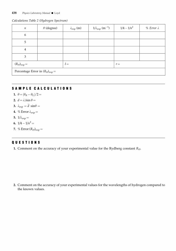
S A M P L E C A L C U L A T I O N S1. y¼ jyR� yLj/2¼2. d¼ l/sin y¼3. lexp ¼ d siny ¼4. %Error lexp¼5. 1/lexp¼6. 1/4� 1/n2¼7. %Error (RH)exp¼
Q U E S T I O N S1. Comment on the accuracy of your experimental value for the Rydberg constant RH.
2. Comment on the accuracy of your experimental values for the wavelengths of hydrogen compared tothe known values.
Calculations Table 2 (Hydrogen Spectrum)
n y (degree) lexp (m) 1/lexp (m�1) 1/4� 1/n2 % Error l
6
5
4
3
(RH)exp¼ I¼ r¼
Percentage Error in (RH)exp¼
438 Physics Laboratory Manual n Loyd

3. State the precision of your determination of the value of the grating spacing d. State clearly the basisfor your answer.
4. Calculate the percentage error of your experimental values of the four wavelengths of hydrogencompared to the Balmer wavelengths you calculated in Question 2 of the Pre-Laboratory.
5. Using the Balmer formula (Equation 1), calculate the n¼ 7 wavelength for the hydrogen spectrum.Why was this wavelength not observed in the laboratory?
COPYRIG
HTª
2008ThomsonBrooks/Cole
Laboratory 43 n Bohr Theory of Hydrogen—The Rydberg Constant 439

This page intentionally left blank
Simulated RadioactiveDecay Using Dice ‘‘Nuclei’’
O B J E C T I V E So Investigate the analogy between the decay of dice ‘‘nuclei’’ and radioactive nuclei.
o Demonstrate that both the number N and activity A of ‘‘nuclei’’ decrease exponentially.
o Determine experimental and theoretical values of the decay probability constant l and the half-life for the dice ‘‘nuclei.’’
E Q U I P M E N T L I S T. 20-sided dice to simulate radioactive nuclei
. Three-cycle semilog graph paper
T H E O R YOne of the most noticeable differences between the classical physics known prior to l900 and the modernphysics since that time is the increased role that probability plays in modern physical theories. The exactbehavior of many physical systems cannot be predicted in advance. Many situations involve a very largenumber of particles inwhich the behavior of any one particle is not predictable, but the average behavior ofthe collection of particles is quite predictable. One example is a sample of radioactive nuclei that emitsalpha, beta, or gamma radiation. It is not possible to predict when any one radioactive nucleus will decayand emit a particle. However, because any reasonable sample of radioactive material contains such a largenumber of nuclei (at least 1012 nuclei), it is possible to predict the average rate of decaywith highprobability.
A basic concept of radioactive decay is that the probability of decay for each radioactive nucleus isconstant. In other words, there are a predictable number of decays per second even though it is notpossible to predict which nuclei among the sample will decay. A quantity called the decay constant lcharacterizes this concept. It is the probability of decay per unit time for one radioactive nucleus. Becausel is constant, it is possible to predict the rate of decay for a radioactive sample. The value of the constant lis different for each radioactive nuclide.
Consider a sample ofN radioactive nuclei with a decay constant of l. The rate of decay of these nucleidN/dt is related to l and N by the equation
dN
dt¼ �lN ðEq: 1Þ
Physics Laboratory Manual n Loyd L A B O R A T O R Y 44
COPYRIG
HTª
2008ThomsonBrooks/Cole
441
ª 2008 Thomson Brooks/Cole, a part of TheThomson Corporation.Thomson, the Star logo, and Brooks/Cole are trademarks used herein under license. ALL RIGHTSRESERVED.No part of this workcovered by the copyright hereonmay be reproduced or used in any form or by any meansçgraphic, electronic, ormechanical, including photocopying, recording, taping,web distribution, informationstorage and retrieval systems,or in any othermannerçwithout the written permission of the publisher.
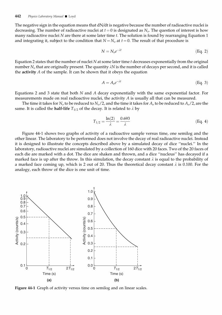
The negative sign in the equationmeans that dN/dt is negative because the number of radioactive nuclei isdecreasing. The number of radioactive nuclei at t¼ 0 is designated as No. The question of interest is howmany radioactive nuclei N are there at some later time t. The solution is found by rearranging Equation 1and integrating it, subject to the condition that N¼No at t¼ 0. The result of that procedure is
N ¼ Noe�lt ðEq: 2Þ
Equation 2 states that the number of nucleiN at some later time t decreases exponentially from the originalnumberNo that are originally present. The quantity lN is the number of decays per second, and it is calledthe activity A of the sample. It can be shown that it obeys the equation
A ¼ Aoe�lt ðEq: 3Þ
Equations 2 and 3 state that both N and A decay exponentially with the same exponential factor. Formeasurements made on real radioactive nuclei, the activity A is usually all that can be measured.
The time it takes forNo to be reduced toNo/2, and the time it takes forAo to be reduced toAo/2, are thesame. It is called the half-life T1/2 of the decay. It is related to l by
T1=2 ¼ lnð2Þl
¼ 0:693
lðEq: 4Þ
Figure 44-1 shows two graphs of activity of a radioactive sample versus time, one semilog and theother linear. The laboratory to be performed does not involve the decay of real radioactive nuclei. Insteadit is designed to illustrate the concepts described above by a simulated decay of dice ‘‘nuclei.’’ In thelaboratory, radioactive nuclei are simulated by a collection of 160 dice with 20 faces. Two of the 20 faces ofeach die are marked with a dot. The dice are shaken and thrown, and a dice ‘‘nucleus’’ has decayed if amarked face is up after the throw. In this simulation, the decay constant l is equal to the probability ofa marked face coming up, which is 2 out of 20. Thus the theoretical decay constant l is 0.100. For theanalogy, each throw of the dice is one unit of time.
0.1 0.0
0.1
0.2
0.3
0.4
0.5
0.6
0.7
0.8
0.9
1.0
0
Time (s)
Act
ivity
(co
unts
/s)
Act
ivity
(co
unts
/s)
(a)
T1/2 2T1/2 0
Time (s)
(b)
T1/2 2T1/2
0.2
0.3
0.4
0.5
0.60.70.80.91.0
Figure 44-1 Graph of activity versus time on semilog and on linear scales.
442 Physics Laboratory Manual n Loyd
A unique aspect of this simulation laboratory is that measurements can be taken on both the numberremaining N and the number that decay. The number that decay is analogous to the activity A. For realradioactive nuclei, N cannot be measured directly but is inferred from measurements of A, the activity.
E X P E R I M E N T A L P R O C E D U R E1. Place all 160 of the dice in the square plastic tray provided with the dice. Place the clear plastic cover
over the dice and shake them vigorously. Remove all dice that come to rest with a marked face up.Remove only those that have a marked face that points directly upward. Record in Data andCalculations Table 1 the number of dice that decay (are removed) on the first throw of the dice. Alsorecord the number of dice that remain after the ones that decay are removed.
2. Place the cover on the dice and shake the remaining dice vigorously. Remove the dice that come to restwith a marked face up on the second throw. Record in Data and Calculations Table 1 the number ofdice removed on the second throw, and also record the number of dice that remain after the ones thatdecay are removed.
3. Continue this process of shaking the dice, removing the ones that have a marked face up, andrecording the number of dice removed and the number of dice left for each throw. Continue thisprocedure for a total of 20 throws of the dice, or until all of the dice have been removed.
4. Each experimental group should record its data on the blackboard so that the class results can beplotted as a set of data with better statistics. Sum the total number of dice thrown originally for theentire class and sum the number removed at each throw of the dice. Record this class data in DataTable 2.
G R A P H S1. On three-cycle semilog graph paper provided by the instructor, graph the results. Plot N the number
of ‘‘nuclei’’ remaining on the log scale versus the number of throws on the linear scale, using� as asymbol. On the same piece of graph paper, plot the activityA (number removed each throw) on the logscale versus the number of throws on the linear scale, usingþ for a symbol.
2. On a second piece of three-cycle semilog graph paper, graph the class data for N and A. With betterstatistics, these curves should be smoother than the individual data.
3. If the dice behaved exactly according to the theory described, all of the graphs described above wouldfall on a straight line on the semilog plot. The data for N will most likely show this trend better thanthe data for A.
4. For the individual data and the class data, draw a straight line that best fits the data. Do this for bothNand A.
C A L C U L A T I O N S1. For each of the 20 shakes of the dice, calculate the ratio of the number of dice removed after a given
throw to the number shaken for that throw. In the simulation the number of dice removed is A, theactivity, and the number shaken isN, the number of radioactive nuclei. Thus these ratios amount to anexperimental value for l. Note carefully that this ratio must be calculated with data from two differentrows in Data and Calculations Table 1. For example, the number of dice thrown on the fourth throw islisted as the number of dice remaining after the third throw. Thus the ratio is calculated with thenumber removed on each row to the number remaining in the preceding row. Record these 20 valuesas lexp in Data and Calculations Table 1.C
OPYRIG
HTª
2008ThomsonBrooks/Cole
Laboratory 44 n Simulated Radioactive Decay Using Dice ‘‘Nuclei’’ 443

2. Calculate the mean of these 20 values for lexp and record it in Calculations Table 2 as lexp.
3. The theoretical value of l is 0.100. Record this value in Calculations Table 2 as ltheo.
4. Calculate the percentage error in the value of lexp compared to ltheo. Record this percentage error inCalculations Table 2.
5. Calculate the theoretical half-life from Equation 4 using the value of l¼ 0.100. Record that value inCalculations Table 2 as (T1/2)theo. For purposes of this calculation consider a fractional throw aspossible.
6. Consider the straight line drawn through the data points of your individual data forN versus numberof throws. The experimental half-life is the number of throws needed to go from any point on the lineto one-half that value. Determine the number of throws needed to go from 120 to 60 on the straight linethrough your data. Record that number in Calculations Table 2 as (T1/2)exp. For purposes of thisdetermination, consider a fractional throw as possible.
7. Calculate the percentage error in the value (T1/2)exp compared to the value of (T1/2)theo. Record thatpercentage error in Calculations Table 2.
444 Physics Laboratory Manual n Loyd

Name . . . . . . . . . . . . . . . . . . . . . . . . . . . . . . . . . . . . . . . . . . . . . . . . . . . . . . . . . . . . . . . . . . . . . . . . . Section . . . . . . . . . . . . . . . . Date . . . . . . . . . . . . . . . .
44 L A B O R A T O R Y 4 4 Simulated Radioactive Decay Using Dice ‘‘Nuclei’’
P R E - L A B O R A T O R Y A S S I G N M E N T1. A typical sample of radioactive material would contain as a lower limit approximately how many
nuclei? (a) 1000 (b) 106 (c) 1012 (d) 1023
2. The theory of radioactive decay can predict when each of the radioactive nuclei in a sample will decay.(a) True (b) False
3. State the definition of the decay constant l. What are its units?
4. For the simulation of a radioactive decay using 20-sided dice, what are the analogous quantities to thereal quantities listed below?
undecayed nucleus—
decayed nucleus—
time—
decay constant—
5. What quantity can be measured for the simulation laboratory that cannot normally be directlymeasured in a true radioactive decay laboratory?
COPYRIG
HTª
2008ThomsonBrooks/Cole
445

6. A radioactive decay process has a decay constant l¼ 1.50� 10�4 sec�1. There are 5.00� 1012 radio-active nuclei in the sample at t¼ 0. How many radioactive nuclei are present in the sample one hourlater? Show your work.
7. For the radioactive sample described in Question 6, what is the activity A (in decays per second)at t¼ 0? What is the activity one hour later? Show your work.
8. What is the half-life of the radioactive sample described in Question 6? Show your work.
446 Physics Laboratory Manual n Loyd

Name . . . . . . . . . . . . . . . . . . . . . . . . . . . . . . . . . . . . . . . . . . . . . . . . . . . . . . . . . . . . . . . . . . . . . . . . . Section . . . . . . . . . . . . . . . . Date . . . . . . . . . . . . . . . .
Lab Partners . . . . . . . . . . . . . . . . . . . . . . . . . . . . . . . . . . . . . . . . . . . . . . . . . . . . . . . . . . . . . . . . . . . . . . . . . . . . . . . . . . . . . . . . . . . . . . . . . . . . . . . . . . . . . . . . . . . .
44 L A B O R A T O R Y 4 4 Simulated Radioactive Decay Using Dice ‘‘Nuclei’’
L A B O R A T O R Y R E P O R T
COPYRIG
HTª
2008ThomsonBrooks/Cole
Data and Calculations Table 1
Throw Removed (A) Remaining (N)
lexp0 0 160
1
2
3
4
5
6
7
8
9
10
11
12
13
14
15
16
Data Table 2
Removed (A) Remaining (N)
0
(Continued)
447
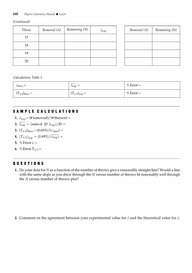
S A M P L E C A L C U L A T I O N S1. lexp¼ (# removed)/(# thrown)¼2. lexp ¼ ðsumof 20 lexpÞ=20 ¼3. (T1/2)theo¼ (0.693)/(l theo)¼4. ðT1/2Þexp ¼ ð0:693Þ=ðlexpÞ ¼5. %Error l¼6. %Error T1/2¼
Q U E S T I O N S1. Do your data forN as a function of the number of throws give a reasonably straight line? Would a line
with the same slope as you drew through the N versus number of throws fit reasonably well throughthe A versus number of throws plot?
2. Comment on the agreement between your experimental value for l and the theoretical value for l.
Throw Removed (A) Remaining (N) lexp
17
18
19
20
Removed (A) Remaining (N)
(Continued)
Calculations Table 2
ltheo¼ lexp ¼ %Error¼
(T1/2)theo¼ (T1/2)exp¼ %Error¼
448 Physics Laboratory Manual n Loyd

3. Comment on the agreement between your experimental value for the half-life and the theoreticalvalue of the half-life.
4. Are the graphs for the class data smoother and more nearly a straight line than your individual data?Would you expect this to be true, and if so, why?
5. Calculate the half-life from the class data graph. Compare it to the theoretical value for the half-life.Would you expect it to show better agreement, and if so, why?
COPYRIG
HTª
2008ThomsonBrooks/Cole
Laboratory 44 n Simulated Radioactive Decay Using Dice ‘‘Nuclei’’ 449

This page intentionally left blank
Geiger Counter Measurementof the Half-Life of 137Ba
O B J E C T I V E So Measure the count rate versus voltage for a Geiger counter to determine its appropriate operating
voltage.
o Measure the activity of 137Ba as a function of time to determine its half-life.
E Q U I P M E N T L I S T. Geiger counter, scaler, timer, 90Sr beta radiation source
. Minigenerator that produces 137Ba from the decay of a parent nuclide of 137Cs
. Disposable plachet (very thin small metal plate to contain a radioactive sample)
. Three-cycle semilog graph paper
T H E O R YA basic concept of radioactive decay is that the probability of decay for each radioactive nucleus isconstant. In other words, there are a predictable number of decays per second even though it is notpossible to predict which nuclei among the sample will decay. A quantity called the decay constant lcharacterizes this concept. It is the probability of decay per unit time for one radioactive nucleus. Becausel is constant, it is possible to predict the rate of decay for a radioactive sample. The value of the constant lis different for each radioactive nuclide.
Consider a sample ofN radioactive nuclei with a decay constant of l. The rate of decay of these nucleidN/dt is related to l and N by the equation
dN
dt¼ �lN ðEq: 1Þ
The negative sign in the equationmeans that dN/dt is negative because the number of radioactive nuclei isdecreasing. The number of radioactive nuclei at t¼ 0 is designated as No. The question of interest is howmany radioactive nuclei N are there at some later time t. The solution is found by rearranging Equation 1and integrating it, subject to the condition that N¼No at t¼ 0. The result of that procedure is
N ¼ Noe�lt ðEq: 2Þ
Physics Laboratory Manual n Loyd L A B O R A T O R Y 45
COPYRIG
HTª
2008ThomsonBrooks/Cole
451
ª 2008 Thomson Brooks/Cole, a part of TheThomson Corporation.Thomson, the Star logo, and Brooks/Cole are trademarks used herein under license. ALL RIGHTSRESERVED.No part of this workcovered by the copyright hereonmay be reproduced or used in any form or by any meansçgraphic, electronic, ormechanical, including photocopying, recording, taping,web distribution, informationstorage and retrieval systems,or in any othermannerçwithout the written permission of the publisher.
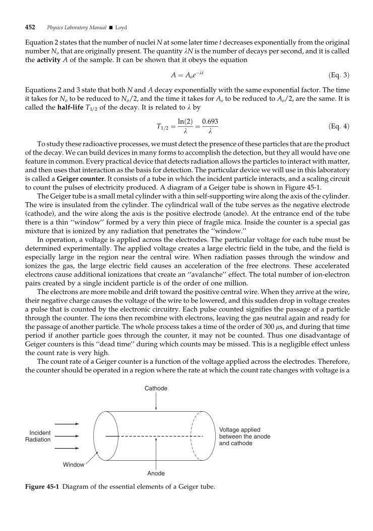
Equation 2 states that the number of nucleiN at some later time t decreases exponentially from the originalnumberNo that are originally present. The quantity lN is the number of decays per second, and it is calledthe activity A of the sample. It can be shown that it obeys the equation
A ¼ Aoe�lt ðEq: 3Þ
Equations 2 and 3 state that both N and A decay exponentially with the same exponential factor. The timeit takes for No to be reduced to No/2, and the time it takes for Ao to be reduced to Ao/2, are the same. It iscalled the half-life T1/2 of the decay. It is related to l by
T1=2 ¼ lnð2Þl
¼ 0:693
lðEq: 4Þ
To study these radioactive processes,wemust detect the presence of these particles that are the productof the decay.We can build devices in many forms to accomplish the detection, but they all would have onefeature in common. Every practical device that detects radiation allows the particles to interact withmatter,and then uses that interaction as the basis for detection. The particular device wewill use in this laboratoryis called aGeiger counter. It consists of a tube in which the incident particle interacts, and a scaling circuitto count the pulses of electricity produced. A diagram of a Geiger tube is shown in Figure 45-1.
TheGeiger tube is a smallmetal cylinderwith a thin self-supportingwire along the axis of the cylinder.The wire is insulated from the cylinder. The cylindrical wall of the tube serves as the negative electrode(cathode), and the wire along the axis is the positive electrode (anode). At the entrance end of the tubethere is a thin ‘‘window’’ formed by a very thin piece of fragile mica. Inside the counter is a special gasmixture that is ionized by any radiation that penetrates the ‘‘window.’’
In operation, a voltage is applied across the electrodes. The particular voltage for each tube must bedetermined experimentally. The applied voltage creates a large electric field in the tube, and the field isespecially large in the region near the central wire. When radiation passes through the window andionizes the gas, the large electric field causes an acceleration of the free electrons. These acceleratedelectrons cause additional ionizations that create an ‘‘avalanche’’ effect. The total number of ion-electronpairs created by a single incident particle is of the order of one million.
The electrons are moremobile and drift toward the positive central wire. When they arrive at the wire,their negative charge causes the voltage of the wire to be lowered, and this sudden drop in voltage createsa pulse that is counted by the electronic circuitry. Each pulse counted signifies the passage of a particlethrough the counter. The ions then recombine with electrons, leaving the gas neutral again and ready forthe passage of another particle. The whole process takes a time of the order of 300 ms, and during that timeperiod if another particle goes through the counter, it may not be counted. Thus one disadvantage ofGeiger counters is this ‘‘dead time’’ during which counts may be missed. This is a negligible effect unlessthe count rate is very high.
The count rate of a Geiger counter is a function of the voltage applied across the electrodes. Therefore,the counter should be operated in a region where the rate at which the count rate changes with voltage is a
Cathode
AnodeWindow
IncidentRadiation
Voltage appliedbetween the anodeand cathode
Figure 45-1 Diagram of the essential elements of a Geiger tube.
452 Physics Laboratory Manual n Loyd
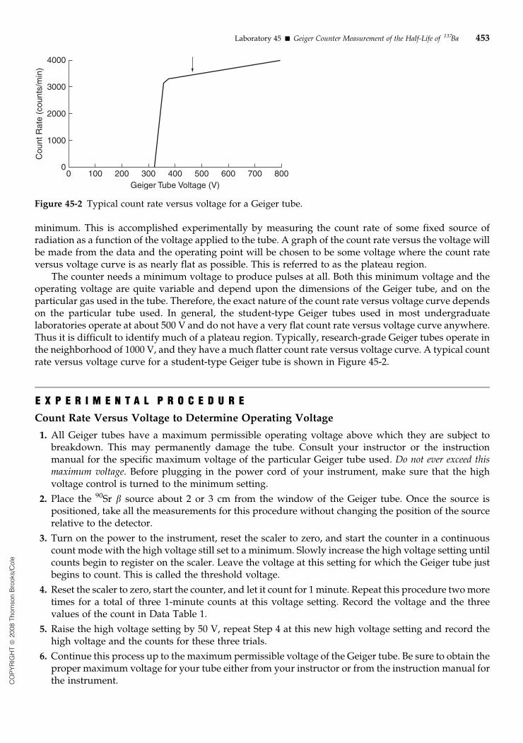
minimum. This is accomplished experimentally by measuring the count rate of some fixed source ofradiation as a function of the voltage applied to the tube. A graph of the count rate versus the voltage willbe made from the data and the operating point will be chosen to be some voltage where the count rateversus voltage curve is as nearly flat as possible. This is referred to as the plateau region.
The counter needs a minimum voltage to produce pulses at all. Both this minimum voltage and theoperating voltage are quite variable and depend upon the dimensions of the Geiger tube, and on theparticular gas used in the tube. Therefore, the exact nature of the count rate versus voltage curve dependson the particular tube used. In general, the student-type Geiger tubes used in most undergraduatelaboratories operate at about 500 V and do not have a very flat count rate versus voltage curve anywhere.Thus it is difficult to identify much of a plateau region. Typically, research-grade Geiger tubes operate inthe neighborhood of 1000 V, and they have a much flatter count rate versus voltage curve. A typical countrate versus voltage curve for a student-type Geiger tube is shown in Figure 45-2.
E X P E R I M E N T A L P R O C E D U R ECount Rate Versus Voltage to Determine Operating Voltage
1. All Geiger tubes have a maximum permissible operating voltage above which they are subject tobreakdown. This may permanently damage the tube. Consult your instructor or the instructionmanual for the specific maximum voltage of the particular Geiger tube used. Do not ever exceed thismaximum voltage. Before plugging in the power cord of your instrument, make sure that the highvoltage control is turned to the minimum setting.
2. Place the 90Sr b source about 2 or 3 cm from the window of the Geiger tube. Once the source ispositioned, take all the measurements for this procedure without changing the position of the sourcerelative to the detector.
3. Turn on the power to the instrument, reset the scaler to zero, and start the counter in a continuouscount mode with the high voltage still set to a minimum. Slowly increase the high voltage setting untilcounts begin to register on the scaler. Leave the voltage at this setting for which the Geiger tube justbegins to count. This is called the threshold voltage.
4. Reset the scaler to zero, start the counter, and let it count for 1 minute. Repeat this procedure twomoretimes for a total of three 1-minute counts at this voltage setting. Record the voltage and the threevalues of the count in Data Table 1.
5. Raise the high voltage setting by 50 V, repeat Step 4 at this new high voltage setting and record thehigh voltage and the counts for these three trials.
6. Continue this process up to the maximum permissible voltage of the Geiger tube. Be sure to obtain theproper maximum voltage for your tube either from your instructor or from the instruction manual forthe instrument.C
OPYRIG
HTª
2008ThomsonBrooks/Cole
00 100 200 300 400
Geiger Tube Voltage (V)
Cou
nt R
ate
(cou
nts/
min
)
500 600 700 800
1000
2000
3000
4000
Figure 45-2 Typical count rate versus voltage for a Geiger tube.
Laboratory 45 n Geiger Counter Measurement of the Half-Life of 137Ba 453
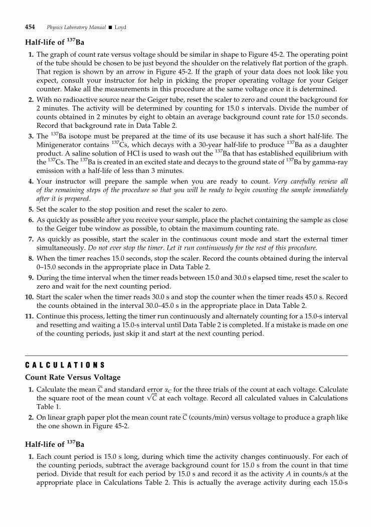
Half-life of 137Ba
1. The graph of count rate versus voltage should be similar in shape to Figure 45-2. The operating pointof the tube should be chosen to be just beyond the shoulder on the relatively flat portion of the graph.That region is shown by an arrow in Figure 45-2. If the graph of your data does not look like youexpect, consult your instructor for help in picking the proper operating voltage for your Geigercounter. Make all the measurements in this procedure at the same voltage once it is determined.
2. With no radioactive source near the Geiger tube, reset the scaler to zero and count the background for2 minutes. The activity will be determined by counting for 15.0 s intervals. Divide the number ofcounts obtained in 2 minutes by eight to obtain an average background count rate for 15.0 seconds.Record that background rate in Data Table 2.
3. The 137Ba isotope must be prepared at the time of its use because it has such a short half-life. TheMinigenerator contains 137Cs, which decays with a 30-year half-life to produce 137Ba as a daughterproduct. A saline solution of HCl is used to wash out the 137Ba that has established equilibrium withthe 137Cs. The 137Ba is created in an excited state and decays to the ground state of 137Ba by gamma-rayemission with a half-life of less than 3 minutes.
4. Your instructor will prepare the sample when you are ready to count. Very carefully review allof the remaining steps of the procedure so that you will be ready to begin counting the sample immediatelyafter it is prepared.
5. Set the scaler to the stop position and reset the scaler to zero.
6. As quickly as possible after you receive your sample, place the plachet containing the sample as closeto the Geiger tube window as possible, to obtain the maximum counting rate.
7. As quickly as possible, start the scaler in the continuous count mode and start the external timersimultaneously. Do not ever stop the timer. Let it run continuously for the rest of this procedure.
8. When the timer reaches 15.0 seconds, stop the scaler. Record the counts obtained during the interval0–15.0 seconds in the appropriate place in Data Table 2.
9. During the time interval when the timer reads between 15.0 and 30.0 s elapsed time, reset the scaler tozero and wait for the next counting period.
10. Start the scaler when the timer reads 30.0 s and stop the counter when the timer reads 45.0 s. Recordthe counts obtained in the interval 30.0–45.0 s in the appropriate place in Data Table 2.
11. Continue this process, letting the timer run continuously and alternately counting for a 15.0-s intervaland resetting and waiting a 15.0-s interval until Data Table 2 is completed. If a mistake is made on oneof the counting periods, just skip it and start at the next counting period.
C A L C U L A T I O N SCount Rate Versus Voltage
1. Calculate the mean C and standard error aC for the three trials of the count at each voltage. Calculatethe square root of the mean count
ffiffiffiffiC
pat each voltage. Record all calculated values in Calculations
Table 1.
2. On linear graph paper plot the mean count rate C (counts/min) versus voltage to produce a graph likethe one shown in Figure 45-2.
Half-life of 137Ba
1. Each count period is 15.0 s long, during which time the activity changes continuously. For each ofthe counting periods, subtract the average background count for 15.0 s from the count in that timeperiod. Divide that result for each period by 15.0 s and record it as the activity A in counts/s at theappropriate place in Calculations Table 2. This is actually the average activity during each 15.0-s
454 Physics Laboratory Manual n Loyd

time interval, but it will be assumed that it approximates the instantaneous activity at the middleof each time interval.
2. Calculate the quantities (Ao/A) and ln (Ao/A) for each of the activities in Data Table 2 whereAo is takento be the activity at t¼ 0.
3. The quantity ln (Ao/A) should vary linearly with t the time, and the slope should be equal to thedisintegration constant l. Perform a linear least squares fit of the data in Calculations Table 2 withln (Ao/A) as the vertical axis and t the time as the horizontal. Record the value of the slope as thedisintegration constant l in Calculations Table 2.
4. Using Equation 4, calculate the experimental value of the half-life of 137Ba from the experimental valueof the disintegration constant l.
G R A P H SHalf-life of 137Ba
1. On three-cycle semilog graph paper, plot the activity in counts/second versus the time in seconds,using the log scale for the activity and the linear scale for time. Graph each activity at the timecorresponding to the middle of the time interval as given in Calculations Table 2.
COPYRIG
HTª
2008ThomsonBrooks/Cole
Laboratory 45 n Geiger Counter Measurement of the Half-Life of 137Ba 455

This page intentionally left blank
Name . . . . . . . . . . . . . . . . . . . . . . . . . . . . . . . . . . . . . . . . . . . . . . . . . . . . . . . . . . . . . . . . . . . . . . . . . Section . . . . . . . . . . . . . . . . Date . . . . . . . . . . . . . . . .
45 L A B O R A T O R Y 4 5 Geiger Counter Measurement of the Half-Life of 137Ba
P R E - L A B O R A T O R Y A S S I G N M E N T1. For the isotope of the element nickel 28
63Ni give the number of protons Z, the number of neutrons N,and the mass number A.
2. Show that Equation 3 in the laboratory can be expressed in the form ln(Ao/A)¼ lt. This is the formused to fit the data in the laboratory.
3. What is the basis for the detection of the particles from any radioactive decay?
4. The inside of a Geiger tube is filled with a (a) gas (b) liquid (c) solid (d) plasma.
5. The pulse that is counted in a Geiger tube is caused by a (a) rise in voltage from ions arriving at theanode (b) drop in the voltage from ions arriving at the anode (c) rise in voltage from electrons arrivingat the anode (d) drop in voltage from electrons arriving at the anode.
6. In a Geiger tube the total time taken to create a pulse and then let the electrons recombinewith the ionsto again form a neutral state is about (a) 1 ms (b) 30 ms (c) 300 ms (d) 10,000 ms.
COPYRIG
HTª
2008ThomsonBrooks/Cole
457

7. A typical operating voltage for a Geiger counter is about (a) 5 V (b) 50 V (c) 500 V (d) 5000 V.
8. In this laboratory the half-life of 137Ba will be determined by measuring (a) the number of atoms leftas a function of time (b) the activity that is constant (c) the activity that decreases as a function of time(d) the activity that increases as a function of time.
458 Physics Laboratory Manual n Loyd

Name . . . . . . . . . . . . . . . . . . . . . . . . . . . . . . . . . . . . . . . . . . . . . . . . . . . . . . . . . . . . . . . . . . . . . . . . . Section . . . . . . . . . . . . . . . . Date . . . . . . . . . . . . . . . .
Lab Partners . . . . . . . . . . . . . . . . . . . . . . . . . . . . . . . . . . . . . . . . . . . . . . . . . . . . . . . . . . . . . . . . . . . . . . . . . . . . . . . . . . . . . . . . . . . . . . . . . . . . . . . . . . . . . . . . . . . .
45 L A B O R A T O R Y 4 5 Geiger Counter Measurement of the Half-Life of 137Ba
L A B O R A T O R Y R E P O R T
COPYRIG
HTª
2008ThomsonBrooks/Cole
Data Table 1
Voltage Count 1 Count 2 Count 3
Calculations Table 1
C aCffiffiffiffiC
p
459
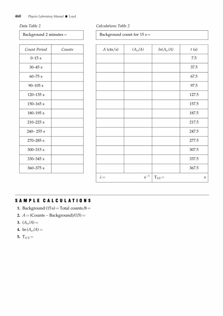
S A M P L E C A L C U L A T I O N S1. Background (15 s)¼Total counts/8¼2. A¼ (Counts�Background)/(15)¼3. (Ao/A)¼4. ln (Ao/A)¼5. T1/2¼
Calculations Table 2
Background count for 15 s¼
A (cts/s) (Ao/A) ln(Ao/A) t (s)
7.5
37.5
67.5
97.5
127.5
157.5
187.5
217.5
247.5
277.5
307.5
337.5
367.5
l¼ s�1 T1/2¼ s
Data Table 2
Background 2 minutes¼
Count Period Counts
0–15 s
30–45 s
60–75 s
90–105 s
120–135 s
150–165 s
180–195 s
210–225 s
240– 255 s
270–285 s
300–315 s
330–345 s
360–375 s
460 Physics Laboratory Manual n Loyd
Q U E S T I O N S1. For the count rate versus voltage data consider the standard error aC and the square root of the mean
countffiffiffiffiC
p. According to nuclear statistical theory, those quantities should be approximately equal.
Calculate the percentage difference between them.
2. State the threshold voltage (voltage at which the counter begins to operate) for your Geiger tube.
3. On the semilog graph of the activity of 137Ba, draw the best straight line that you can through the datapoints. From the straight line determine the half-life of the sample. Indicate exactly which points onthe straight line are used to determine the half-life.
4. The accepted half-life of 137Ba is 2.6 min. Calculate the percentage error of each of your determinationsof this half-life. Show your work.
5. A physics professor purchased a 137Cs source in September 1990, which had an activity of 2.00� 105
disintegrations per second at that time. What is the activity of that source today? (The half-life of 137Csis 30.2 years.) Show your work.
COPYRIG
HTª
2008ThomsonBrooks/Cole
Laboratory 45 n Geiger Counter Measurement of the Half-Life of 137Ba 461

This page intentionally left blank

Nuclear Counting Statistics
O B J E C T I V E So Investigate the counts from a radioactive source for 50 measurements under conditions in which
the count rate should be approximately constant.
o Determine the standard deviation from the mean and standard error of the counts.
o Investigate how well the observed distribution of counts compares to that predicted by thenormal distribution.
o Investigate whether or notffiffiffiffiC
papproximates the standard deviation from the mean.
E Q U I P M E N T L I S T. Geiger counter (single unit containing Geiger tube, power supply, timer, and scaler)
. Long-lived radioactive source (such as 137Cs or 60Co)
T H E O R YIf all other sources of error are removed from a nuclear counting experiment, there remains an uncertaintydue to the random nature of the nuclear decay process. It is assumed that there exists some true meanvalue of the count, which shall be designated as m. But we emphasize, do not assume that there is a truevalue for any individual count Ci. Although m is assumed to exist, it can never be known exactly. Instead,one can approach knowledge of the true mean m by a large number of observations. It can be shown thatthe best approximation to the true mean m is the mean C, which is given by
C ¼ ð1=nÞXni¼1
Ci ðEq: 1Þ
where Ci stands for the ith value of the count obtained in n trials. The standard deviation from the meansn�1 and the standard error a are defined in the usual manner as
sn�1 ¼ffiffiffiffiffiffiffiffiffiffiffiffiffiffiffiffiffiffiffiffiffiffiffiffiffiffiffiffiffiffiffiffiffiffiffiffiffiffiffiffiffiffiffiffiffiffiXni¼1
ð1=n� 1ÞðC� CiÞ2s
and a ¼ sn�1ffiffiffin
p ðEq: 2Þ
These equations have been applied to essentially all of the measurements in this laboratory manual.In many of the cases where these ideas have been applied, they are somewhat questionable because the
Physics Laboratory Manual n Loyd L A B O R A T O R Y 46
COPYRIG
HTª
2008ThomsonBrooks/Cole
463
ª 2008 Thomson Brooks/Cole, a part of TheThomson Corporation.Thomson, the Star logo, and Brooks/Cole are trademarks used herein under license. ALL RIGHTSRESERVED.No part of this workcovered by the copyright hereonmay be reproduced or used in any form or by any meansçgraphic, electronic, ormechanical, including photocopying, recording, taping,web distribution, informationstorage and retrieval systems,or in any othermannerçwithout the written permission of the publisher.
random errors are not necessarily the determining factor. For nuclear counting experiments, usually therandom errors are the limiting factor, and these concepts generally do apply strictly to suchmeasurements.
The way in which the measurements Ci are distributed around the mean C depends upon thestatistical distribution. The binomial distribution is the fundamental law for the statistics of all randomevents including radioactive decay. Calculations are difficult with this distribution, and it is oftenapproximated by another integral distribution called the Poisson distribution. For cases of m greater than20, both the binomial and the Poisson distribution can be approximated by the normal distribution. Ithas the advantage that it deals with continuous variables, and thus calculations are much easier with thenormal distribution. For most nuclear counting problems of interest, the normal distribution predictsthe same results for nuclear counting that have been assumed for measurements in general.Approximately 68.3% of the measured values of Ci should fall within C� sn�1, and approximately95.5% of the measured values of Ci should fall within C� 2 sn�1.
There is one statistical idea valid for nuclear counting experiments that is not true for measurementsin general. For any given single measurement of the count C in a nuclear counting experiment, anapproximation to the standard deviation from the mean sn�1 is given by
sn�1 �ffiffiffiffiC
pðEq: 3Þ
For a series of repeated trials of a given count, the most accurate determination is given by C� a.If only a single measurement of the count is made, the most accurate statement that can be made isgiven by C� ffiffiffiffi
Cp
.In this laboratory, we will take a series of measurements of the same count to determine the distri-
bution of the measurements about the mean. In addition, we will investigate the validity of Equation 3.
E X P E R I M E N T A L P R O C E D U R E1. Consult your instructor for the operating voltage of the Geiger counter and set the Geiger counter to
the proper operating voltage. Place a long-lived radioactive isotope on whichever counting shelf isnecessary to produce between 500 and 700 counts in a 30 s counting period. For best results, the Geigercounter should have preset timing capabilities. If it does not and a laboratory timer is used, it wouldimprove the timing precision if 60 s counting intervals are used. For whatever time is counted,between 500 and 700 counts should be recorded.
464 Physics Laboratory Manual n Loyd
Image not available due to copyright restrictions

2. Repeat the count for a total of 50 trials. Make no changes whatsoever in the experimental arrangementfor these 50 trials. Record each count in the Data Table. Do not make any background subtraction.Simply record the total count for each counting period.
C A L C U L A T I O N S1. Calculate the mean count C, the standard deviation from the mean sn�1, and the standard error a for
the 50 trials of the count and record the results in the Calculations Table.
2. For each count Ci calculate jCi�Cj=sn�1 and record the results in the Calculations Table.
3. Determine what percentage of the counts Ci are further from C than sn�1 by counting the number oftimes a value of jCi�Cj=sn�1 > 1 occurs. Express this number divided by 50 as a percentage. Countthe number of times that jCi�Cj=sn�1 > 2 occurs. Express this number divided by 50 as a percentage.Record these results in the Calculations Table.
4. CalculateffiffiffiffiC
pand record its value in the Calculations Table.
G R A P H S1. Construct a histogram of your data on linear graph paper. Consider the range of the data and
arbitrarily divide the range into about 15 segments. For counts in the range used, this should giveintervals of 8 or 10 counts. An example of some data is displayed in this manner in Figure 46-2. Themean of the data is 659 with sn�1¼ 27, and an interval of 10 has been chosen.
COPYRIG
HTª
2008ThomsonBrooks/Cole
0590 600 610 620 630 640 650 660
Count Range
Num
ber
of T
imes
Cou
nt in
Giv
en R
ange
670 680 690 700 710 720 730
1
2
3
4
5
6
7
8
9
10
Figure 46-2 Histogram of 50 repeated counts with mean of 659.
Laboratory 46 n Nuclear Counting Statistics 465

This page intentionally left blank
Name . . . . . . . . . . . . . . . . . . . . . . . . . . . . . . . . . . . . . . . . . . . . . . . . . . . . . . . . . . . . . . . . . . . . . . . . . Section . . . . . . . . . . . . . . . . Date . . . . . . . . . . . . . . . .
46 L A B O R A T O R Y 4 6 Nuclear Counting Statistics
P R E - L A B O R A T O R Y A S S I G N M E N T1. For nuclear counting experiments no true value of a given count is assumed. What quantity is
assumed to have a true value?
2. What is the exact statistical distribution function that describes the statistics of nuclear countingexperiments?
3. What statistical distribution function approximates nuclear counting statistics and is used because itdeals with continuous variables? For what values of the true mean m is this distribution valid?
4. In a nuclear counting experiment a single measurement of C counts is obtained. What is the approxi-mate value for sn�1 for the count C?
COPYRIG
HTª
2008ThomsonBrooks/Cole
467
5. According to the normal distribution function,when a given count is repeated 30 times, approximatelyhow many of the results should fall in the range C� sn�1? How many should fall in the rangeC� 2sn�1?
6. A single count of a radioactive nucleus is made, and the result is 927 counts. What is the approximatevalue of sn�1?
7. A set of 10 repeated measurements of the count from a given radioactive sample was taken. Theresults were: 633, 666, 599, 651, 654, 690, 660, 659, 664, and 612. What is the mean count C? What is thevalue of sn�1? What is the value of a? Which of the counts fall outside C� sn�1? Is this approximatelythe number of cases expected? Show your work.
8. For the data in Question 7, isffiffiffiffiC
papproximately equal to sn�1? Calculate the percentage difference
between the two. Show your work.
468 Physics Laboratory Manual n Loyd

Name . . . . . . . . . . . . . . . . . . . . . . . . . . . . . . . . . . . . . . . . . . . . . . . . . . . . . . . . . . . . . . . . . . . . . . . . . Section . . . . . . . . . . . . . . . . Date . . . . . . . . . . . . . . . .
Lab Partners . . . . . . . . . . . . . . . . . . . . . . . . . . . . . . . . . . . . . . . . . . . . . . . . . . . . . . . . . . . . . . . . . . . . . . . . . . . . . . . . . . . . . . . . . . . . . . . . . . . . . . . . . . . . . . . . . . . .
46 L A B O R A T O R Y 4 6 Nuclear Counting Statistics
L A B O R A T O R Y R E P O R T
COPYRIG
HTª
2008ThomsonBrooks/Cole
Data Table
i Ci
1
2
3
4
5
6
7
8
9
10
11
12
13
14
15
16
17
i Ci
18
19
20
21
22
23
24
25
26
27
28
29
30
31
32
33
34
Calculations Table
i jCi�Cj=sn�1
1
2
3
4
5
6
7
8
9
10
11
12
13
14
15
16
17
i jCi�Cj=sn�1
18
19
20
21
22
23
24
25
26
27
28
29
30
31
32
33
34
(Continued)
469

S A M P L E C A L C U L A T I O N S1. jCi�Cj=sn�1 ¼2.
ffiffiffiffiC
p¼
3. % trial > sn�1 from mean¼4. % trial > 2 sn�1 from mean¼
Q U E S T I O N S1. Consider the shape of the histogram of your data. Does it show the expected distribution relative to
the mean of the data?
i Ci
35
36
37
38
39
40
41
42
i Ci
43
44
45
46
47
48
49
50
i jCi�Cj=sn�1
35
36
37
38
39
40
41
42
i jCi�Cj=sn�1
43
44
45
46
47
48
49
50
C¼ sn�1¼
a¼ffiffiffiffiC
p¼
% trial >sn�1 from mean¼
% trial > 2 sn�1 from mean¼
(Continued)
470 Physics Laboratory Manual n Loyd
2. Compare the percentage of trials that have jCi�Cj=sn�1 > 1 with that predicted by the normaldistribution. Compare the percentage of trials that have jCi�Cj=sn�1 > 2 with that predicted by thenormal distribution.
3. What is the most accurate statement that you can make about the count from the sample based uponthe data that you have taken?
4. Calculate the percentage difference betweenffiffiffiffiC
pand sn�1. Do the results confirm the expectations of
Equation 3?
COPYRIG
HTª
2008ThomsonBrooks/Cole
Laboratory 46 n Nuclear Counting Statistics 471

This page intentionally left blank

Absorption of Beta andGamma Rays
O B J E C T I V E So Investigate the difference in relative absorption by different types of materials for different kinds
of radiation.
o Determine the absorption coefficient m for gamma radiation in lead.
E Q U I P M E N T L I S T. Geiger counter (single unit with Geiger tube, power supply, timer, and scaler)
. Absorber set (lead and polyethylene), two-cycle semilog graph paper
. Gamma source (60Co, for example), beta source (90Sr, for example)
T H E O R YThree different particles are emitted in the three types of natural radioactivity. In a-decay the emittedparticle is a twice-ionized helium atom called an alpha particle. In b-decay the emitted particle isan electron or positron. For c-decay the emitted particle is a high-energy photon. The different natureof these particles accounts for the differences in their relative absorption in matter. The most importantcharacteristics that determine the interactions are the charge and the mass of the particles. Because theyare charged and have large mass, alpha particles interact very strongly, lose energy in a series ofinteractions, and do not travel far in matter. For a typical a-decay the particle will not penetrate the thinwindow of a Geiger counter. Therefore we will use no a-decay sources in this laboratory.
Because the g-ray photons have no mass or charge, they interact with matter in a fundamentallydifferent way than charged particles interact. They interact less strongly with matter, and as a result arethe most penetrating type of radiation. They require a greater thickness of material to be completelyabsorbed. Gamma rays interact with matter by the photoelectric effect, the Compton effect, and bypositron-electron pair production. In each of these processes a photon is effectively completely removedfrom the beam in a single process, if it interacts at all. The consequence of this fact, that photons either donot interact at all or else are completely removed by an interaction, means that g-ray intensity decreasesexponentially with absorber thickness. Photons are the only particles from natural radioactivity to interactin this manner, and are the only ones to show an exact exponential decrease in matter.
Physics Laboratory Manual n Loyd L A B O R A T O R Y 47
COPYRIG
HTª
2008ThomsonBrooks/Cole
473
ª 2008 Thomson Brooks/Cole, a part of TheThomson Corporation.Thomson, the Star logo, and Brooks/Cole are trademarks used herein under license. ALL RIGHTSRESERVED.No part of this workcovered by the copyright hereonmay be reproduced or used in any form or by any meansçgraphic, electronic, ormechanical, including photocopying, recording, taping,web distribution, informationstorage and retrieval systems,or in any othermannerçwithout the written permission of the publisher.
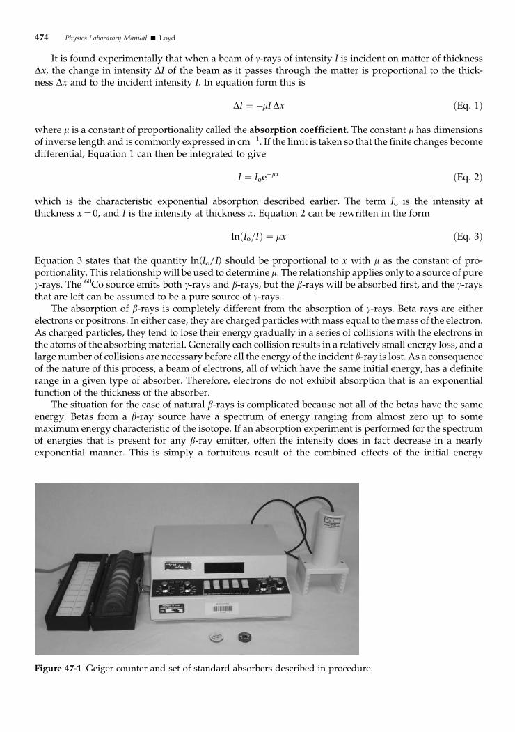
It is found experimentally that when a beam of g-rays of intensity I is incident on matter of thicknessDx, the change in intensity DI of the beam as it passes through the matter is proportional to the thick-ness Dx and to the incident intensity I. In equation form this is
DI ¼ �mI Dx ðEq: 1Þ
where m is a constant of proportionality called the absorption coefficient. The constant m has dimensionsof inverse length and is commonly expressed in cm�1. If the limit is taken so that the finite changes becomedifferential, Equation 1 can then be integrated to give
I ¼ Ioe�mx ðEq: 2Þ
which is the characteristic exponential absorption described earlier. The term Io is the intensity atthickness x¼ 0, and I is the intensity at thickness x. Equation 2 can be rewritten in the form
lnðIo=IÞ ¼ mx ðEq: 3Þ
Equation 3 states that the quantity ln(Io/I) should be proportional to x with m as the constant of pro-portionality. This relationshipwill be used to determine m. The relationship applies only to a source of pureg-rays. The 60Co source emits both g-rays and b-rays, but the b-rays will be absorbed first, and the g-raysthat are left can be assumed to be a pure source of g-rays.
The absorption of b-rays is completely different from the absorption of g-rays. Beta rays are eitherelectrons or positrons. In either case, they are charged particles withmass equal to themass of the electron.As charged particles, they tend to lose their energy gradually in a series of collisions with the electrons inthe atoms of the absorbingmaterial. Generally each collision results in a relatively small energy loss, and alarge number of collisions are necessary before all the energy of the incident b-ray is lost. As a consequenceof the nature of this process, a beam of electrons, all of which have the same initial energy, has a definiterange in a given type of absorber. Therefore, electrons do not exhibit absorption that is an exponentialfunction of the thickness of the absorber.
The situation for the case of natural b-rays is complicated because not all of the betas have the sameenergy. Betas from a b-ray source have a spectrum of energy ranging from almost zero up to somemaximum energy characteristic of the isotope. If an absorption experiment is performed for the spectrumof energies that is present for any b-ray emitter, often the intensity does in fact decrease in a nearlyexponential manner. This is simply a fortuitous result of the combined effects of the initial energy
Figure 47-1 Geiger counter and set of standard absorbers described in procedure.
474 Physics Laboratory Manual n Loyd
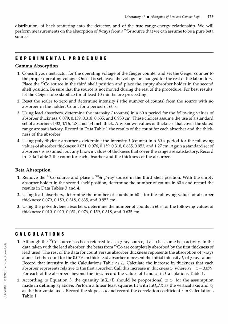
distribution, of back scattering into the detector, and of the true range-energy relationship. We willperformmeasurements on the absorption of b-rays from a 90Sr source that we can assume to be a pure betasource.
E X P E R I M E N T A L P R O C E D U R EGamma Absorption
1. Consult your instructor for the operating voltage of the Geiger counter and set the Geiger counter tothe proper operating voltage. Once it is set, leave the voltage unchanged for the rest of the laboratory.Place the 60Co source in the third shelf position and place the empty absorber holder in the secondshelf position. Be sure that the source is not moved during the rest of the procedure. For best results,let the Geiger tube stabilize for at least 10 min before proceeding.
2. Reset the scaler to zero and determine intensity I (the number of counts) from the source with noabsorber in the holder. Count for a period of 60 s.
3. Using lead absorbers, determine the intensity I (counts) in a 60 s period for the following values ofabsorber thickness: 0.079, 0.159. 0.318, 0.635, and 0.953 cm. These choices assume the use of a standardset of absorbers 1/32, 1/16, 1/8, and 1/4 inch thick. Any known values of thickness that cover the statedrange are satisfactory. Record in Data Table 1 the results of the count for each absorber and the thick-ness of the absorber.
4. Using polyethylene absorbers, determine the intensity I (counts) in a 60 s period for the followingvalues of absorber thickness: 0.051, 0.076, 0.159, 0.318, 0.635, 0.953, and 1.27 cm. Again a standard set ofabsorbers is assumed, but any known values of thickness that cover the range are satisfactory. Recordin Data Table 2 the count for each absorber and the thickness of the absorber.
Beta Absorption
1. Remove the 60Co source and place a 90Sr b-ray source in the third shelf position. With the emptyabsorber holder in the second shelf position, determine the number of counts in 60 s and record theresults in Data Tables 3 and 4.
2. Using lead absorbers, determine the number of counts in 60 s for the following values of absorberthickness: 0.079, 0.159, 0.318, 0.635, and 0.953 cm.
3. Using the polyethylene absorbers, determine the number of counts in 60 s for the following values ofthickness: 0.010, 0.020, 0.051, 0.076, 0.159, 0.318, and 0.635 cm.
C A L C U L A T I O N S1. Although the 60Co source has been referred to as a g-ray source, it also has some beta activity. In the
data takenwith the lead absorber, the betas from 60Co are completely absorbed by the first thickness oflead used. The rest of the data for count versus absorber thickness represents the absorption of g-raysalone. Let the count for the 0.079 cm thick lead absorber represent the initial intensity Io of g-rays alone.Record that intensity in the Calculations Table as Io. Calculate the increase in thickness that eachabsorber represents relative to the first absorber. Call this increase in thickness x1 where x1¼ x� 0.079.For each of the absorbers beyond the first, record the values of I and x1 in Calculations Table 1.
2. According to Equation 3, the quantity ln(Io/I) should be proportional to x1 for the assumptionmade in defining x1 above. Perform a linear least squares fit with ln(Io/I) as the vertical axis and x1as the horizontal axis. Record the slope as m and record the correlation coefficient r in CalculationsTable 1.C
OPYRIG
HTª
2008ThomsonBrooks/Cole
Laboratory 47 n Absorption of Beta and Gamma Rays 475
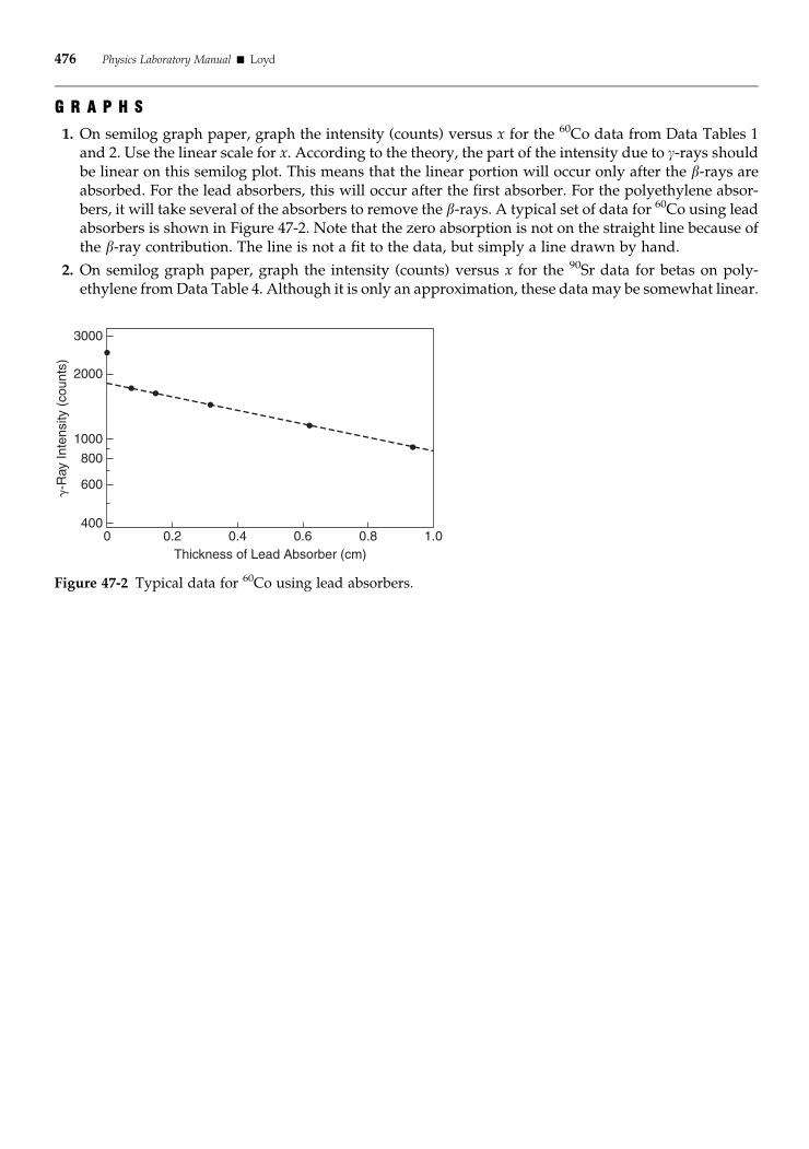
G R A P H S1. On semilog graph paper, graph the intensity (counts) versus x for the 60Co data from Data Tables 1
and 2. Use the linear scale for x. According to the theory, the part of the intensity due to g-rays shouldbe linear on this semilog plot. This means that the linear portion will occur only after the b-rays areabsorbed. For the lead absorbers, this will occur after the first absorber. For the polyethylene absor-bers, it will take several of the absorbers to remove the b-rays. A typical set of data for 60Co using leadabsorbers is shown in Figure 47-2. Note that the zero absorption is not on the straight line because ofthe b-ray contribution. The line is not a fit to the data, but simply a line drawn by hand.
2. On semilog graph paper, graph the intensity (counts) versus x for the 90Sr data for betas on poly-ethylene fromData Table 4. Although it is only an approximation, these data may be somewhat linear.
4000 0.2 0.4
Thickness of Lead Absorber (cm)0.6 0.8 1.0
600
800
1000
2000
3000
�-R
ay In
tens
ity (
coun
ts)
Figure 47-2 Typical data for 60Co using lead absorbers.
476 Physics Laboratory Manual n Loyd

Name . . . . . . . . . . . . . . . . . . . . . . . . . . . . . . . . . . . . . . . . . . . . . . . . . . . . . . . . . . . . . . . . . . . . . . . . . Section . . . . . . . . . . . . . . . . Date . . . . . . . . . . . . . . . .
47 L A B O R A T O R Y 4 7 Absorption of Beta and Gamma Rays
P R E - L A B O R A T O R Y A S S I G N M E N T1. What are the names of the three types of natural radioactivity? Describe the nature of the particle
produced in each.
2. Which kind of nuclear radiation undergoes a true exponential absorption as a function of absorberthickness? What property of its interaction with matter causes this to happen?
3. Which kind of natural radioactivity produces particles with a continuous spectrum of energy?
4. Which type of natural radioactivity produces particles that penetrate matter the least? What charac-teristics of these particles cause them to be stopped in less matter?
COPYRIG
HTª
2008ThomsonBrooks/Cole
477

5. State the form of the equation for the absorption of g-rays in matter. Define all the terms used in theequation.
6. What type of radiation is the most penetrating? What properties of the particles from this radiationcause them to penetrate matter so well?
7. Apure g-ray source has a count rate of 5000 counts in oneminute with no absorber between the sourceand the detector. An absorber of thickness 0.375 cm is placed between the source and the detector.The number of counts in the detector in 1 minute is now 3245. What is the absorption coefficient m ofthe material? Show your work.
8. In the experimental arrangement of Question 7, if an additional 0.235 cm of the same material isplaced between the detector and source, what is now the count in 1 minute? Show your work.
478 Physics Laboratory Manual n Loyd

Name . . . . . . . . . . . . . . . . . . . . . . . . . . . . . . . . . . . . . . . . . . . . . . . . . . . . . . . . . . . . . . . . . . . . . . . . . Section . . . . . . . . . . . . . . . . Date . . . . . . . . . . . . . . . .
Lab Partners . . . . . . . . . . . . . . . . . . . . . . . . . . . . . . . . . . . . . . . . . . . . . . . . . . . . . . . . . . . . . . . . . . . . . . . . . . . . . . . . . . . . . . . . . . . . . . . . . . . . . . . . . . . . . . . . . . . .
47 L A B O R A T O R Y 4 7 Absorption of Beta and Gamma Rays
L A B O R A T O R Y R E P O R T
COPYRIG
HTª
2008ThomsonBrooks/Cole
Data Table 1 g-rays on Lead
x (cm) I (counts)
0
Data Table 3 b-rays on Lead
x (cm) I (counts)
0
Data Table 2 g-rays on Polyethylene
x (cm) I (counts)
0
Data Table 4 b-rays on Polyethylene
x (cm) I (counts)
0
479
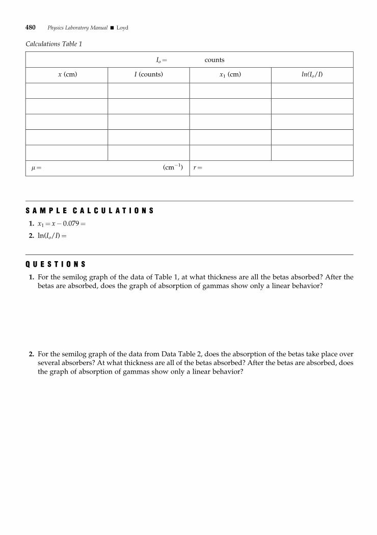
Calculations Table 1
Io¼ counts
x (cm) I (counts) x1 (cm) ln(Io/I)
m¼ (cm�1) r¼
S A M P L E C A L C U L A T I O N S1. x1¼ x� 0.079¼2. ln(Io/I)¼
Q U E S T I O N S1. For the semilog graph of the data of Table 1, at what thickness are all the betas absorbed? After the
betas are absorbed, does the graph of absorption of gammas show only a linear behavior?
2. For the semilog graph of the data from Data Table 2, does the absorption of the betas take place overseveral absorbers? At what thickness are all of the betas absorbed? After the betas are absorbed, doesthe graph of absorption of gammas show only a linear behavior?
480 Physics Laboratory Manual n Loyd

3. Comment on the data in Data Table 3 for the intensity of 90Sr radiation versus the thickness of leadabsorber. What is your conclusion about the absorption of betas in lead?
4. Comment on the semilog graph of the data from Data Table 4 for the intensity of 90Sr radiation versusthickness of polyethylene absorber. Is the graph approximately linear? If it is not linear over the wholerange, is it at least linear over some portion of the range?
5. For gammas of the approximate energy of the 60Co gammas in lead, the approximate value of theabsorption coefficient is m¼ 0.65 cm�1. Considering this as the accepted value, calculate the accuracyof your measurement of m.
COPYRIG
HTª
2008ThomsonBrooks/Cole
Laboratory 47 n Absorption of Beta and Gamma Rays 481

This page intentionally left blank

Correlation Coefficients*
This table shows the probability of obtaining a given correlation coefficient r for two variables for whichthere is in fact no correlation. This probability is a strong function of the number of data points n. As anillustration of the table, consider the case of n¼ 12. There is a 10% probability of obtaining a value ofr� 0.497, a 2% probability of obtaining a value of r� 0.658, and a 0.1% probability of obtaining a value ofr� 0.823 for data for which no actual correlation exists. For many cases in the laboratory manual, you willtake data that produce values of r greater than the 0.1% probability for the particular value of n. In thosecases, one can conclude that the data are very strong evidence for a linear relationship between the variables.
Physics Laboratory Manual n Loyd A P P E N D I X I
COPYRIG
HTª
2008ThomsonBrooks/Cole
*This table is adapted from Table VI of Fisher and Yates, Statistical Tables for Biological, Agricultural, and MedicalResearch, published by Oliver & Boyd, Ltd., Edinburgh, by permission of the authors and publishers.
Probability (%)
n 10 5 2 1 0.1
3 0.988 0.997 0.999 1.000 1.000
4 0.900 0.950 0.980 0.990 0.999
5 0.805 0.878 0.934 0.959 0.992
6 0.729 0.811 0.882 0.917 0.974
7 0.669 0.754 0.833 0.874 0.951
8 0.621 0.707 0.789 0.834 0.925
9 0.582 0.666 0.750 0.798 0.898
10 0.549 0.632 0.716 0.765 0.872
11 0.521 0.602 0.685 0.735 0.847
12 0.497 0.576 0.658 0.708 0.823
15 0.441 0.514 0.592 0.641 0.760
20 0.378 0.444 0.516 0.561 0.679
483
ª 2008 Thomson Brooks/Cole, a part of TheThomson Corporation.Thomson, the Star logo, and Brooks/Cole are trademarks used herein under license. ALL RIGHTSRESERVED.No part of this workcovered by the copyright hereonmay be reproduced or used in any form or by any meansçgraphic, electronic, ormechanical, including photocopying, recording, taping,web distribution, informationstorage and retrieval systems,or in any othermannerçwithout the written permission of the publisher.

This page intentionally left blank

Properties of Materials
Physics Laboratory Manual n Loyd A P P E N D I X II
COPYRIG
HTª
2008ThomsonBrooks/Cole
Table II A Density of Substances (kg/m3)
Substance Density Substance Density
Aluminum 2.7� 103 Cork 0.22� 0.26� 103
Brass 8.4� 103 Oak wood 0.60� 0.90� 103
Copper 8.9� 103 Maple wood 0.62� 0.75� 103
Gold 19.3� 103 Pine wood 0.35� 0.50� 103
Iron 7.85� 103 Alcohol, ethyl 0.79� 103
Lead 11.3� 103 Alcohol, methyl 0.81� 103
Nickel 8.7� 103 Mercury 13.6� 103
Steel 7.8� 103 Pure water 1.000� 103
Zinc 7.1� 103 Sea water 1.025� 103
Table II B Specific Heats (Calories/gram�C8)
Substance Specific Heat Substance Specific Heat
Aluminum 0.22 Mercury 0.033
Brass 0.092 Steel 0.12
Copper 0.093 Tin 0.054
Iron 0.11 Water 1.000
Lead 0.031 Zinc 0.093
485
ª 2008 Thomson Brooks/Cole, a part of TheThomson Corporation.Thomson, the Star logo, and Brooks/Cole are trademarks used herein under license. ALL RIGHTSRESERVED.No part of this workcovered by the copyright hereonmay be reproduced or used in any form or by any meansçgraphic, electronic, ormechanical, including photocopying, recording, taping,web distribution, informationstorage and retrieval systems,or in any othermannerçwithout the written permission of the publisher.

Table II C Thermal Coefficients of Expansion (C8)�1
Substance a Substance a
Aluminum 24� 10�6 Brass and bronze 19� 10�6
Copper 17� 10�6 Lead 29� 10�6
Pyrex glass 3.2� 10�6 Ordinary glass 9� 10�6
Steel 11� 10�6 Concrete 12� 10�6
Gold 14� 10�6 Tin 27� 10�6
Table II D Resistivities and Temperature Coefficients
Substance Resistivity(O�m) Temperature Coefficient (C8)�1
Aluminum 2.82� 10�8 3.9� 10�3
Copper 1.72� 10�8 3.9� 10�3
Silver 1.59� 10�8 3.8� 10�3
Gold 2.44� 10�8 3.4� 10�3
Nickel-silver 33� 10�8 0.4� 10�3
Tungsten 5.6� 10�8 4.5� 10�3
Iron 10� 10�8 5.0� 10�3
Lead 22� 10�8 3.9� 10�3
Carbon 3.5� 10�5 �0.5� 10�3
486 Physics Laboratory Manual n Loyd
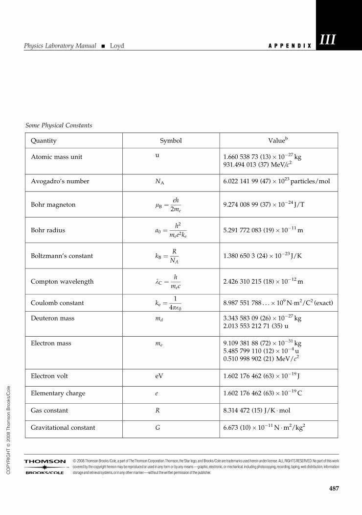
Physics Laboratory Manual n Loyd A P P E N D I X III
COPYRIG
HTª
2008ThomsonBrooks/Cole
Some Physical Constants
Quantity Symbol Valueb
Atomic mass unit u 1.660 538 73 (13)� 10�27 kg931.494 013 (37) MeV/c2
Avogadro’s number NA 6.022 141 99 (47)� 1023 particles/mol
Bohr magneton mB ¼ eh
2me9.274 008 99 (37)� 10�24 J/T
Bohr radius a0 ¼ h2
mee2ke5.291 772 083 (19)� 10�11m
Boltzmann’s constant kB ¼ R
NA1.380 650 3 (24)� 10�23 J/K
Compton wavelength lC ¼ h
mec2.426 310 215 (18)� 10�12m
Coulomb constant ke ¼ 1
4p�08.987 551 788 . . .� 109N�m2/C2 (exact)
Deuteron mass md 3.343 583 09 (26)� 10�27 kg2.013 553 212 71 (35) u
Electron mass me 9.109 381 88 (72)� 10�31 kg5.485 799 110 (12)� 10�4 u0.510 998 902 (21) MeV/c2
Electron volt eV 1.602 176 462 (63)� 10�19 J
Elementary charge e 1.602 176 462 (63)� 10�19 C
Gas constant R 8.314 472 (15) J/K �mol
Gravitational constant G 6.673 (10)� 10�11N �m2/kg2
487
ª 2008 Thomson Brooks/Cole, a part of TheThomson Corporation.Thomson, the Star logo, and Brooks/Cole are trademarks used herein under license. ALL RIGHTSRESERVED.No part of this workcovered by the copyright hereonmay be reproduced or used in any form or by any meansçgraphic, electronic, ormechanical, including photocopying, recording, taping,web distribution, informationstorage and retrieval systems,or in any othermannerçwithout the written permission of the publisher.
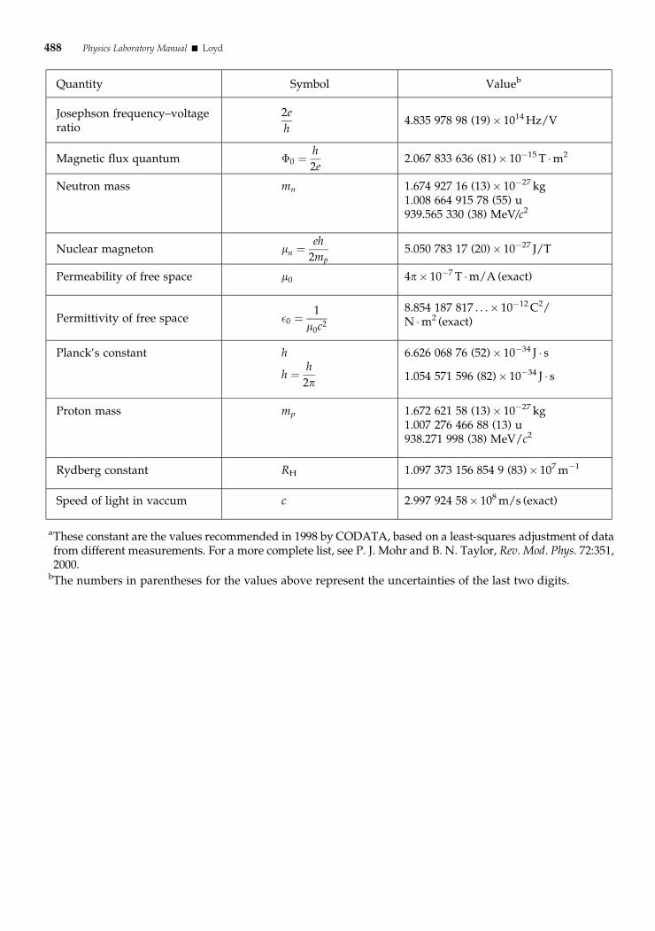
Quantity Symbol Valueb
Josephson frequency–voltageratio
2e
h4.835 978 98 (19)� 1014Hz/V
Magnetic flux quantum �0 ¼ h
2e2.067 833 636 (81)� 10�15 T �m2
Neutron mass mn 1.674 927 16 (13)� 10�27 kg1.008 664 915 78 (55) u939.565 330 (38) MeV/c2
Nuclear magneton mn ¼ eh
2mp5.050 783 17 (20)� 10�27 J/T
Permeability of free space m0 4p� 10�7 T �m/A (exact)
Permittivity of free space �0 ¼ 1
m0c28.854 187 817 . . .� 10�12 C2/N �m2 (exact)
Planck’s constant h
h ¼ h
2p
6.626 068 76 (52)� 10�34 J � s1.054 571 596 (82)� 10�34 J � s
Proton mass mp 1.672 621 58 (13)� 10�27 kg1.007 276 466 88 (13) u938.271 998 (38) MeV/c2
Rydberg constant RH 1.097 373 156 854 9 (83)� 107m�1
Speed of light in vaccum c 2.997 924 58� 108m/s (exact)
aThese constant are the values recommended in 1998 by CODATA, based on a least-squares adjustment of datafrom different measurements. For a more complete list, see P. J. Mohr and B. N. Taylor, Rev. Mod. Phys. 72:351,2000.
bThe numbers in parentheses for the values above represent the uncertainties of the last two digits.
488 Physics Laboratory Manual n Loyd

COPYRIG
HTª
2008ThomsonBrooks/Cole
Solar System Data
Body Mass (kg) Mean Radius (m) Period (s) Distance from the Sun (m)
Mercury 3.18� 1023 2.43� 106 7.60� 106 5.79� 1010
Venus 4.88� 1024 6.06� 106 1.94� 107 1.08� 1011
Earth 5.98� 1024 6.37� 106 3.156� 107 1.496� 1011
Mars 6.42� 1023 3.37� 106 5.94� 107 2.28� 1011
Jupiter 1.90� 1027 6.99� 107 3.74� 108 7.78� 1011
Saturn 5.68� 1026 5.85� 107 9.35� 108 1.43� 1012
Uranus 8.68� 1025 2.33� 107 2.64� 109 2.87� 1012
Neptune 1.03� 1026 2.21� 107 5.22� 109 4.50� 1012
Pluto �1.4� 1022 �1.5� 106 7.82� 109 5.91� 1012
Moon 7.36� 1022 1.74� 106 — —
Sun 1.991� 1030 6.96� 108 — —
Physical Data Often Used
Average Earth-Moon distance 3.84� 108m
Average Earth-Sun distance 1,496� 1011m
Average radius of the Earth 6.37� 106m
Density of air (208C and 1 atm) 1.20 kt/m3
Density of water (208C and 1 atm) 1.00� 103 kg/m3
Free-fall acceleration 9.80 m/s2
Mass of the Earth 5.98� 1024 kg
Mass of the Moon 7.36� 1022 kg
Mass of the Sun 1.99� 1030 kg
Standard atmospheric pressure 1.013� 105 Pa
Appendix III 489

Some Prefixes for Powers of Ten
Power Prefix Abbreviation Power Prefix Abbreviation
10�24 yocto y 101 deka da
10�21 zepto z 102 hecto h
10�18 atto a 103 kilo k
10�15 femto f 106 mega M
10�12 pico p 109 giga G
10�9 nano n 1012 tera T
10�6 micro m 1015 peta P
10�3 milli m 1018 exa E
10�2 centi c 1021 zetta Z
10�1 deci d 1024 yotta Y
490 Physics Laboratory Manual n Loyd

COPYRIG
HTª
2008ThomsonBrooks/Cole
Standard Abbreviations and Symbols for Units
Symbol Unit Symbol Unit
A ampere K kelvin
u atomic mass unit kg kilogram
atm atmophere kmol kilomole
Btu British thermal unit L liter
C coulomb lb pound
8C degree Celsius ly light-year
cal calorie m meter
d day min minute
eV electron volt mol mole
8F degree Fahrenheit N newton
F farad Pa pascal
ft foot rad radian
G gauss rev revolution
g gram s second
H henry T tesla
h hour V volt
hp horsepower W watt
Hz hertz Wb weber
in. inch yr year
J joule O ohm
Appendix III 491
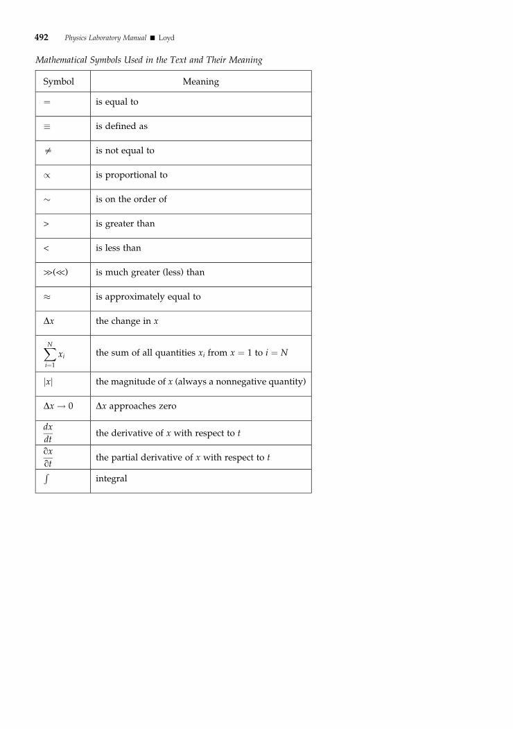
Mathematical Symbols Used in the Text and Their Meaning
Symbol Meaning
¼ is equal to
is defined as
= is not equal to
/ is proportional to
� is on the order of
> is greater than
< is less than
>>(<<) is much greater (less) than
� is approximately equal to
Dx the change in x
XNi¼1
xi the sum of all quantities xi from x ¼ 1 to i ¼ N
jxj the magnitude of x (always a nonnegative quantity)
Dx ! 0 Dx approaches zero
dx
dtthe derivative of x with respect to t
qxqt
the partial derivative of x with respect to tRintegral
492 Physics Laboratory Manual n Loyd

COPYRIG
HTª
2008ThomsonBrooks/Cole
Conversions
Length
1 in.¼ 2.54 cm (exact)
1m¼ 39.37 in.¼ 3.281 ft
1 ft¼ 0.304 8m
12 in.¼ 1 ft
3 ft¼ 1 yd
1 yd¼ 0.914 4m
1km¼ 0.621mi
1mi¼ 1.609 km
1mi¼ 5 280 ft
1 mm¼ 10�6m¼ 103 nm
1 ligh-tyear¼ 9.461� 1015m
Area
1m2¼ 104cm2¼ 10.76 ft2
1 ft2¼ 0.092 9m2¼ 144 in.2
1 in.2¼ 6.452 cm2
Volume
1m3¼ 106cm3¼ 6.102� 104 in.3
1 ft3¼ 1.728 in.3¼ 2.83� 10�2m3
1L¼ 1 000 cm3¼ 1.057 6 qt¼ 0.035 3 ft3
1 ft3¼ 7.481 gal¼ 28.32 L¼ 2.832� 10�2m3
1 gal¼ 3.786L¼ 231 in.3
Mass
100 kg¼ 1 t (metric ton)
1 slug¼ 14.59 kg
1u¼ 1.66� 10�27 kg¼ 931.5MeV/c2
Force
1N¼ 0.224 8 lb
1 lb¼ 4.448N
Velocity
1mi/h¼ 1.47 ft/s¼ 0.447m/s¼ 1.61 km/h
1m/s¼ 100 cm/s¼ 3.281 ft/s
1mi/min¼ 60mi/h¼ 88 ft/s
Acceleration
1m/s2¼ 3.28 ft/s2¼ 100 cm/s2
1 ft/s2¼ 0.304 8m/s2¼ 30.48 cm/s2
Pressure
1 bar¼ 105N/m2¼ 14.50 lb/in.2
1 atm¼ 760mmHg¼ 76.0 cmHg
1 atm¼ 14.7 lb/in.2¼ 1.013� 105N/m2
1Pa¼ 1N/m2¼ 1.45� 10�4 lb/in.2
Time
1 yr¼ 365 days¼ 3.16� 107s
1 day¼ 24 h¼ 1.44� 103min¼ 8.64� 104 s
Energy
1 J¼ 0.738 ft � lb1 cal¼ 4.186 J
1 Btu¼ 252 cal¼ 1.054� 103 J
1 eV¼ 1.6� 10�19 J
1 kWh¼ 3.60� 106 J
Power
1 hp¼ 550 ft�lb/s¼ 0.746 kW
1W¼ 1 J/s¼ 0.738 ft � lb/s1 Btu/h¼ 0.293W
Some Approximations Useful for Estimation Problems
1m� 1 yd
1 kg� 2 lb
1N � 14 lb
1 L � 14 gal
1m/s� 2mi/h
1 yr� p� 107s
60mi/h� 100 ft/s
1 km � 12 mi
Appendix III 493

The Greek Alphabet
Alpha A a Iota I i Rho P r
Beta B b Kappa K k Sigma S s
Gamma G g Lambda L l Tau T t
Delta D d Mu M m Upsilon � u
Epsilon E E Nu N n Phi F f
Zeta Z z Xi X x Chi X w
Eta H Z Omicron O o Psi C c
Theta Y y Pi P p Omega O o
494 Physics Laboratory Manual n Loyd