Physics Letters A 379 (2015) 830–834

Contents lists available at ScienceDirect

Physics Letters A

www.elsevier.com/locate/pla

The Sun is the climate pacemaker II.Global ocean temperatures

David H. Douglass ∗, Robert S. Knox

Department of Physics and Astronomy, University of Rochester, Rochester, NY 14627-0171, United States

a r t i c l e i n f o a b s t r a c t

Article history:Received 27 August 2014Received in revised form 9 October 2014Accepted 10 October 2014Available online 5 December 2014Communicated by V.M. Agranovich

Keywords:ClimateClimatologySolar forcingSeasonal effectsPhase lockingOcean heat content

In part I, equatorial Pacific Ocean temperature index SST3.4 was found to have segments during 1990–2014 showing a phase-locked annual signal and phase-locked signals of 2- or 3-year periods. Phase locking is to an inferred solar forcing of 1.0 cycle/yr. Here the study extends to the global ocean, from surface to 700 and 2000 m. The same phase-locking phenomena are found. The El Niño/La Niña effect diffuses into the world oceans with a delay of about two months.

© 2014 Elsevier B.V. All rights reserved.

1. Introduction

In a study of equatorial Pacific Ocean temperature [1] it was found that phase locking of annual temperature signals with sub-harmonic components occurs at subharmonic periods of two or three years. Ten such segments were identified and numbered se-quentially in the period 1870–2008. Either the beginning date, the end date, or both, of those segments had a near one-to-one cor-respondence with previously reported abrupt climate changes or climate shifts. To explain the various phenomena it was concluded that this climate system is driven by a forcing F S of solar origin at a frequency of 1.0 cycle/yr that causes both the direct-response principal component and the subharmonic response. These, and the 1 cycle/yr component, were phase locked to the annual so-lar cycle. In this study “phase-locked” always refers to the solar cycle as reference.

In the companion Letter [2] we studied the equatorial Pacific surface temperature SST3.4 from 1990 to 2014 and found three segments phase locked at subharmonics of F S . The first two update the result reported in [1]: a 1991–1999 segment showing period-icity of 3 years and a 2002–2008 segment showing periodicity of two years. The third is new: a segment from 2008–2013 (end of data) showing periodicity of three years. Phase locking was deci-sively demonstrated by producing closed Lissajous loops.

* Corresponding author.E-mail address: douglass@pas.rochester.edu (D.H. Douglass).

http://dx.doi.org/10.1016/j.physleta.2014.10.0580375-9601/© 2014 Elsevier B.V. All rights reserved.

Section 2 describes data sets, methods, and background ma-terial. Results are analyzed and discussed in Section 3. Section 4considers related issues and the conclusions are summarized in Section 5.

2. Data and methods

2.1. Data

This study considers only data from January 1990 through De-cember 2013.

HadSST3: A monthly global ocean surface temperature data set HadSST3 is produced by the Met Office Hadley Centre, Exeter, UK [3].

Average global temperature sets for different depths are avail-able [4]. The data set for each depth D will be labeled “TD”. For example, T2000 denotes average global ocean temperature from the surface to a depth of 2000 m. In addition to an average over depths a geographical average is taken over the major oceanic basins: Pacific Ocean, Atlantic Ocean (which includes the entire Arctic Ocean), and the Indian Ocean. These data are quarterly (4 values/yr). The designation of quarters will be with a suffix. For example, the first quarter, Jan/Feb/Mar of 2000 is written as 2000-1; Apr/May/Jun of 2000 as 2000-2; etc.

2.2. Separation of high- and low-frequency effects

Studies of many geophysical phenomena involve data sets con-taining a component of interest that may show components at

D.H. Douglass, R.S. Knox / Physics Letters A 379 (2015) 830–834 831

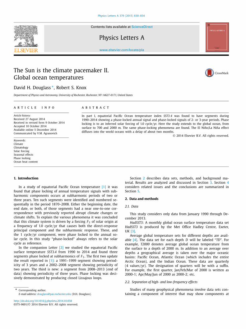
Fig. 1. Plots associated with HadSST3. a. Plot of HadSST3 (black, with data points) and aHadSST3 (red). The 24-month and 36-month phase-locked segments are indicated by green shaded rectangles. b. Plot of high-frequency component hHadSST3 (lower curve) and its amplitude A(hHadSST3). c. Autocorrelation of hHadSST3 indicating a periodicity of 12 months. d. Autocorrelation of segment of aHAdSST3 from February 2002 to March 2008 (in red) and of segment of aSST3.4 from 2008 to the end of available data (2013), indicating, respectively, periodicities of 24 and 36 months. (For interpretation of the references to color in this figure, the reader is referred to the web version of this article.)

frequencies of 1.0 cycle/yr and its harmonics. Subharmonics re-lated to non-annual effects such as El Niño/La Niña can also appear. For a full understanding of the data set these compo-nents must be separated. In this paper we continue to use the filter, methodology, and notation described previously. The high-frequency component is denoted by prefix “h” and the low-frequency component by “a”. Thus, for example, we will have hSST3.4, aT700, etc. By definition for any set G these are related by G = hG + aG , point by point. See Appendix A in [2]. Finally, in the present analysis only anomalies are treated. Thus we replace a parent series G0 by G = G0 − 〈G0〉, where 〈G0〉 is the average of the parent series over the period.

2.3. Identifying phase-locked time segments

Geophysical indices aG in which seasonal effects have been re-moved are often found, as in this work, to contain time segments with components having periods that are exactly a multiple of one year. These segments are identified by computing the autocorrela-tion function versus delay time τ of a candidate segment. When there are time segments in aG showing a periodicity of a multi-ple of one year, a complete classification is given by three discrete indices: subharmonic number, parity, and sub-state index [1,2].

In Ref. [2], subharmonic phase locking was demonstrated by showing that aG vs. hG formed a closed Lissajous loop pattern where the number of loops was the subharmonic number. Alas, hG is not available for any of the data sets considered in this Let-

ter because the parent data are not available. For data without hGone must rely only on the autocorrelation test.

It is sometimes useful to consider the amplitude of the high-frequency data series hG , defined as

A(hG) = (2 average

(hG2))1/2

, (1)

where the average is over one year, symmetric about the point in question, and hG2 is the set of squares of the individual numbers in hG .

3. Analysis and discussion

3.1. Global Ocean surface temperatures

HadSST3. The global HadSST3 time series has had the annual cycle supposedly removed by a climatology scheme. Fig. 1a shows HadSST3 (black) and aHadSST3 (red). The fact that the annual ef-fect has not been removed is seen clearly in hHadSST3 (Fig. 1b) and particularly by the autocorrelation of hHadSST3 (Fig. 1c). Also shown in Fig. 1b is the amplitude A(hHadSST3). The autocorrela-tion shows a rapid drop (less than 1 year) from 1.0 to a sustained oscillation of 1.0 cycle/yr of amplitude ∼0.32. The rapid drop is modeled by an exponential decay to the sustained amplitude with a characteristic time te . The best fit was for values of te less than 1.0 year. The red curve is a plot for te = 0.5 years. It is pointed out that although there is an annual component in hHadSST3, it

832 D.H. Douglass, R.S. Knox / Physics Letters A 379 (2015) 830–834

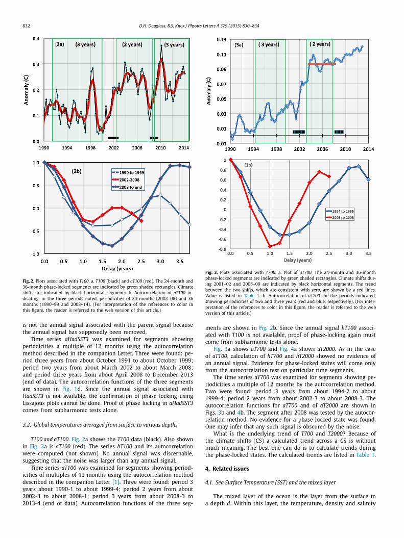
Fig. 2. Plots associated with T100. a. T100 (black) and aT100 (red). The 24-month and 36-month phase-locked segments are indicated by green shaded rectangles. Climate shifts are indicated by black horizontal segments. b. Autocorrelation of aT100 in-dicating, in the three periods noted, periodicities of 24 months (2002–08) and 36 months (1990–99 and 2008–14). (For interpretation of the references to color in this figure, the reader is referred to the web version of this article.)

is not the annual signal associated with the parent signal because the annual signal has supposedly been removed.

Time series aHadSST3 was examined for segments showing periodicities a multiple of 12 months using the autocorrelation method described in the companion Letter. Three were found: pe-riod three years from about October 1991 to about October 1999; period two years from about March 2002 to about March 2008; and period three years from about April 2008 to December 2013 (end of data). The autocorrelation functions of the three segments are shown in Fig. 1d. Since the annual signal associated with HadSST3 is not available, the confirmation of phase locking using Lissajous plots cannot be done. Proof of phase locking in aHadSST3comes from subharmonic tests alone.

3.2. Global temperatures averaged from surface to various depths

T100 and aT100. Fig. 2a shows the T100 data (black). Also shown in Fig. 2a is aT100 (red). The series hT100 and its autocorrelation were computed (not shown). No annual signal was discernable, suggesting that the noise was larger than any annual signal.

Time series aT100 was examined for segments showing period-icities of multiples of 12 months using the autocorrelation method described in the companion Letter [1]. Three were found: period 3 years about 1990-1 to about 1999-4; period 2 years from about 2002-3 to about 2008-1; period 3 years from about 2008-3 to 2013-4 (end of data). Autocorrelation functions of the three seg-

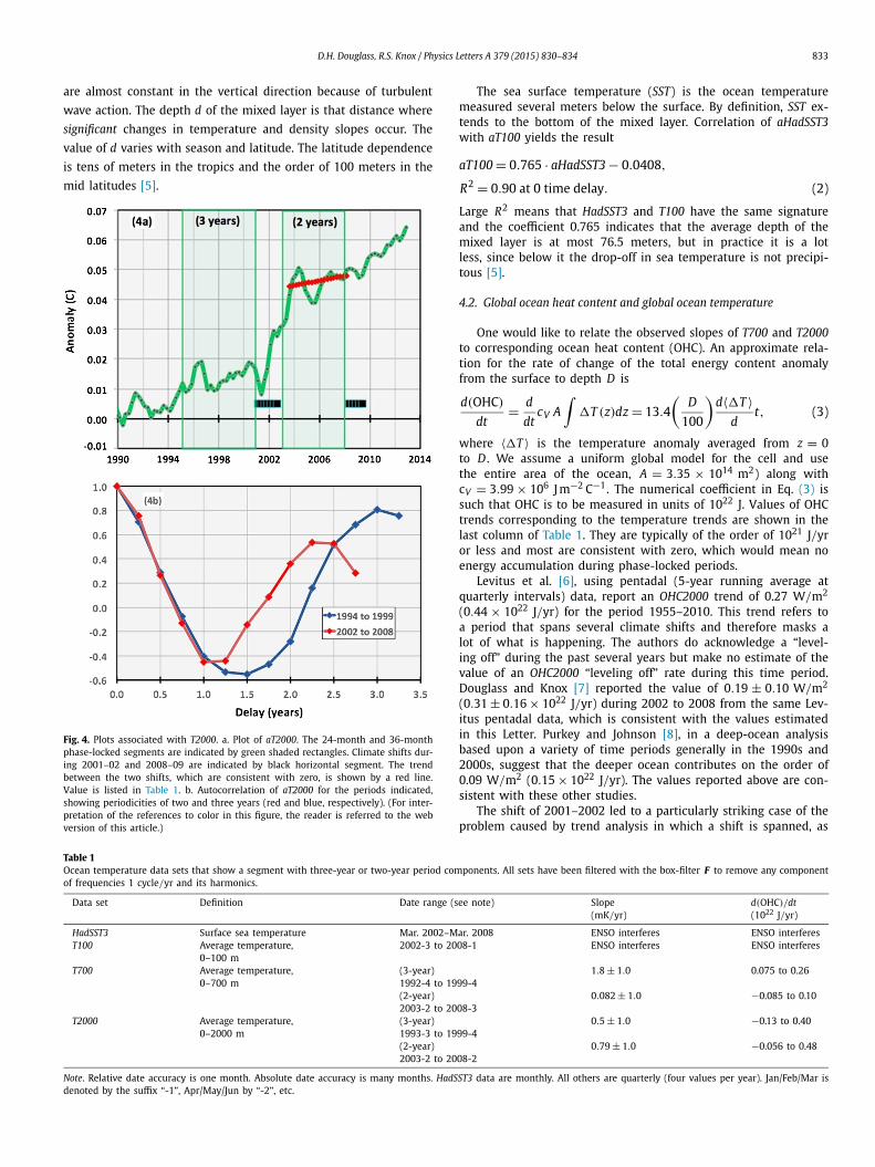
Fig. 3. Plots associated with T700. a. Plot of aT700. The 24-month and 36-month phase-locked segments are indicated by green shaded rectangles. Climate shifts dur-ing 2001–02 and 2008–09 are indicated by black horizontal segments. The trend between the two shifts, which are consistent with zero, are shown by a red lines. Value is listed in Table 1. b. Autocorrelation of aT700 for the periods indicated, showing periodicities of two and three years (red and blue, respectively). (For inter-pretation of the references to color in this figure, the reader is referred to the web version of this article.)

ments are shown in Fig. 2b. Since the annual signal hT100 associ-ated with T100 is not available, proof of phase-locking again must come from subharmonic tests alone.

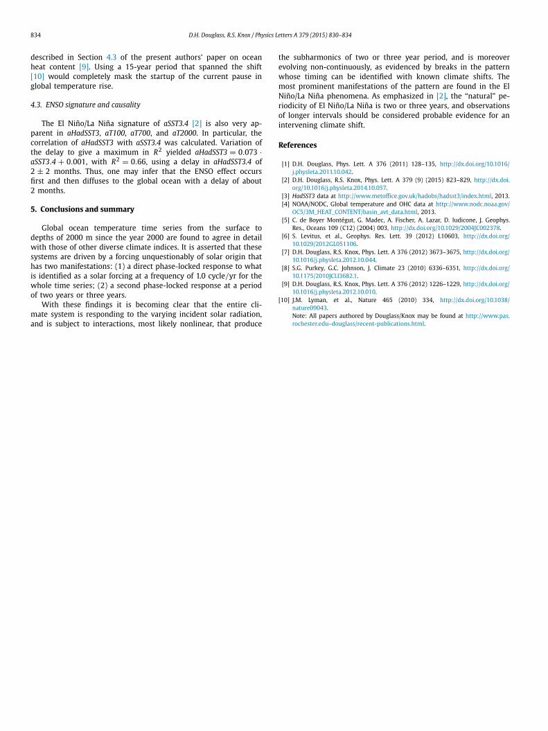
Fig. 3a shows aT700 and Fig. 4a shows aT2000. As in the case of aT100, calculation of hT700 and hT2000 showed no evidence of an annual signal. Evidence for phase-locked states will come only from the autocorrelation test on particular time segments.

The time series aT700 was examined for segments showing pe-riodicities a multiple of 12 months by the autocorrelation method. Two were found: period 3 years from about 1994-2 to about 1999-4; period 2 years from about 2002-3 to about 2008-3. The autocorrelation functions for aT700 and of aT2000 are shown in Figs. 3b and 4b. The segment after 2008 was tested by the autocor-relation method. No evidence for a phase-locked state was found. One may infer that any such signal is obscured by the noise.

What is the underlying trend of T700 and T2000? Because of the climate shifts (CS) a calculated trend across a CS is without much meaning. The best one can do is to calculate trends during the phase-locked states. The calculated trends are listed in Table 1.

4. Related issues

4.1. Sea Surface Temperature (SST) and the mixed layer

The mixed layer of the ocean is the layer from the surface to a depth d. Within this layer, the temperature, density and salinity

D.H. Douglass, R.S. Knox / Physics Letters A 379 (2015) 830–834 833

are almost constant in the vertical direction because of turbulent wave action. The depth d of the mixed layer is that distance where significant changes in temperature and density slopes occur. The value of d varies with season and latitude. The latitude dependence is tens of meters in the tropics and the order of 100 meters in the mid latitudes [5].

Fig. 4. Plots associated with T2000. a. Plot of aT2000. The 24-month and 36-month phase-locked segments are indicated by green shaded rectangles. Climate shifts dur-ing 2001–02 and 2008–09 are indicated by black horizontal segment. The trend between the two shifts, which are consistent with zero, is shown by a red line. Value is listed in Table 1. b. Autocorrelation of aT2000 for the periods indicated, showing periodicities of two and three years (red and blue, respectively). (For inter-pretation of the references to color in this figure, the reader is referred to the web version of this article.)

The sea surface temperature (SST) is the ocean temperature measured several meters below the surface. By definition, SST ex-tends to the bottom of the mixed layer. Correlation of aHadSST3with aT100 yields the result

aT100 = 0.765 · aHadSST3 − 0.0408,

R2 = 0.90 at 0 time delay. (2)

Large R2 means that HadSST3 and T100 have the same signature and the coefficient 0.765 indicates that the average depth of the mixed layer is at most 76.5 meters, but in practice it is a lot less, since below it the drop-off in sea temperature is not precipi-tous [5].

4.2. Global ocean heat content and global ocean temperature

One would like to relate the observed slopes of T700 and T2000to corresponding ocean heat content (OHC). An approximate rela-tion for the rate of change of the total energy content anomaly from the surface to depth D is

d(OHC)

dt= d

dtcV A

∫�T (z)dz = 13.4

(D

100

)d〈�T 〉

dt, (3)

where 〈�T 〉 is the temperature anomaly averaged from z = 0to D . We assume a uniform global model for the cell and use the entire area of the ocean, A = 3.35 × 1014 m2) along with cV = 3.99 × 106 J m−2 C−1. The numerical coefficient in Eq. (3) is such that OHC is to be measured in units of 1022 J. Values of OHC trends corresponding to the temperature trends are shown in the last column of Table 1. They are typically of the order of 1021 J/yror less and most are consistent with zero, which would mean no energy accumulation during phase-locked periods.

Levitus et al. [6], using pentadal (5-year running average at quarterly intervals) data, report an OHC2000 trend of 0.27 W/m2

(0.44 × 1022 J/yr) for the period 1955–2010. This trend refers to a period that spans several climate shifts and therefore masks a lot of what is happening. The authors do acknowledge a “level-ing off” during the past several years but make no estimate of the value of an OHC2000 “leveling off” rate during this time period. Douglass and Knox [7] reported the value of 0.19 ± 0.10 W/m2

(0.31 ± 0.16 × 1022 J/yr) during 2002 to 2008 from the same Lev-itus pentadal data, which is consistent with the values estimated in this Letter. Purkey and Johnson [8], in a deep-ocean analysis based upon a variety of time periods generally in the 1990s and 2000s, suggest that the deeper ocean contributes on the order of 0.09 W/m2 (0.15 × 1022 J/yr). The values reported above are con-sistent with these other studies.

The shift of 2001–2002 led to a particularly striking case of the problem caused by trend analysis in which a shift is spanned, as

Table 1Ocean temperature data sets that show a segment with three-year or two-year period components. All sets have been filtered with the box-filter F to remove any component of frequencies 1 cycle/yr and its harmonics.

Data set Definition Date range (see note) Slope (mK/yr)

d(OHC)/dt(1022 J/yr)

HadSST3 Surface sea temperature Mar. 2002–Mar. 2008 ENSO interferes ENSO interferesT100 Average temperature,

0–100 m2002-3 to 2008-1 ENSO interferes ENSO interferes

T700 Average temperature, 0–700 m

(3-year) 1992-4 to 1999-4

1.8 ± 1.0 0.075 to 0.26

(2-year) 2003-2 to 2008-3

0.082 ± 1.0 −0.085 to 0.10

T2000 Average temperature, 0–2000 m

(3-year) 1993-3 to 1999-4

0.5 ± 1.0 −0.13 to 0.40

(2-year) 2003-2 to 2008-2

0.79 ± 1.0 −0.056 to 0.48

Note. Relative date accuracy is one month. Absolute date accuracy is many months. HadSST3 data are monthly. All others are quarterly (four values per year). Jan/Feb/Mar is denoted by the suffix “-1”, Apr/May/Jun by “-2”, etc.

834 D.H. Douglass, R.S. Knox / Physics Letters A 379 (2015) 830–834

described in Section 4.3 of the present authors’ paper on ocean heat content [9]. Using a 15-year period that spanned the shift [10] would completely mask the startup of the current pause in global temperature rise.

4.3. ENSO signature and causality

The El Niño/La Niña signature of aSST3.4 [2] is also very ap-parent in aHadSST3, aT100, aT700, and aT2000. In particular, the correlation of aHadSST3 with aSST3.4 was calculated. Variation of the delay to give a maximum in R2 yielded aHadSST3 = 0.073 ·aSST3.4 + 0.001, with R2 = 0.66, using a delay in aHadSST3.4 of 2 ± 2 months. Thus, one may infer that the ENSO effect occurs first and then diffuses to the global ocean with a delay of about 2 months.

5. Conclusions and summary

Global ocean temperature time series from the surface to depths of 2000 m since the year 2000 are found to agree in detail with those of other diverse climate indices. It is asserted that these systems are driven by a forcing unquestionably of solar origin that has two manifestations: (1) a direct phase-locked response to what is identified as a solar forcing at a frequency of 1.0 cycle/yr for the whole time series; (2) a second phase-locked response at a period of two years or three years.

With these findings it is becoming clear that the entire cli-mate system is responding to the varying incident solar radiation, and is subject to interactions, most likely nonlinear, that produce

the subharmonics of two or three year period, and is moreover evolving non-continuously, as evidenced by breaks in the pattern whose timing can be identified with known climate shifts. The most prominent manifestations of the pattern are found in the El Niño/La Niña phenomena. As emphasized in [2], the “natural” pe-riodicity of El Niño/La Niña is two or three years, and observations of longer intervals should be considered probable evidence for an intervening climate shift.

References

[1] D.H. Douglass, Phys. Lett. A 376 (2011) 128–135, http://dx.doi.org/10.1016/j.physleta.2011.10.042.

[2] D.H. Douglass, R.S. Knox, Phys. Lett. A 379 (9) (2015) 823–829, http://dx.doi.org/10.1016/j.physleta.2014.10.057.

[3] HadSST3 data at http://www.metoffice.gov.uk/hadobs/hadsst3/index.html, 2013.[4] NOAA/NODC, Global temperature and OHC data at http://www.nodc.noaa.gov/

OC5/3M_HEAT_CONTENT/basin_avt_data.html, 2013.[5] C. de Boyer Montégut, G. Madec, A. Fischer, A. Lazar, D. Iudicone, J. Geophys.

Res., Oceans 109 (C12) (2004) 003, http://dx.doi.org/10.1029/2004JC002378.[6] S. Levitus, et al., Geophys. Res. Lett. 39 (2012) L10603, http://dx.doi.org/

10.1029/2012GL051106.[7] D.H. Douglass, R.S. Knox, Phys. Lett. A 376 (2012) 3673–3675, http://dx.doi.org/

10.1016/j.physleta.2012.10.044.[8] S.G. Purkey, G.C. Johnson, J. Climate 23 (2010) 6336–6351, http://dx.doi.org/

10.1175/2010JCLI3682.1.[9] D.H. Douglass, R.S. Knox, Phys. Lett. A 376 (2012) 1226–1229, http://dx.doi.org/

10.1016/j.physleta.2012.10.010.[10] J.M. Lyman, et al., Nature 465 (2010) 334, http://dx.doi.org/10.1038/

nature09043.Note: All papers authored by Douglass/Knox may be found at http://www.pas.rochester.edu~douglass/recent-publications.html.