Embed Size (px)
Citation preview
Phytoplankton communities in temperate rivers
Jacinthe Contant
Thesis submitted to the
Faculty of Graduate and Postdoctoral Studies
University of Ottawa
In partial fulfillment of the requirements for the
M.Sc. degree in the
Ottawa-Carleton Institute of Biology
Specialization in Chemical and Environmental Toxicology
Thèse soumise à la
Faculté des études supérieures et postdoctorales
Université d’Ottawa
en vue de l’obtention de la maîtrise en sciences à
L’Institut de biologie d’Ottawa-Carleton
Spécialisation en toxicologie chimique et environnementale
© Jacinthe Contant, Ottawa, Canada, 2012

To Mom, Dad, and
Rhys
iii
Abstract
The structure of phytoplankton communities was examined seasonally across five rivers with
a focus on small cells and their relative importance. Picophytoplankton (0.2-2 μm),
previously considered insignificant in rivers, reached densities as high as those observed in
lakes and oceans (~ 104-10
5 cells/mL). Their relative importance was not a function of
trophic state with the highest contribution to algal biomass found in the most eutrophic river.
Body size distributions were analyzed from both chlorophyll-a size fractions and taxonomic
enumerations; no significant effect of river or season was detected, suggesting that
phytoplankton size distribution is not a useful metric of change in rivers. Unlike lake
ecosystems, the rivers were uniformly dominated by small cells (< 20 μm). Taxonomic
analyses of the seasonal succession did not reveal a common periodicity of particular
divisions (e.g. diatoms). However, strong dominance was more typical of eutrophic rivers
even though taxa richness was similar.
iv
Résumé
La structure des communautés phytoplanctoniques a été examinée de mai à novembre dans
cinq rivières tempérées avec une attention particulière portée aux petites cellules et à leur
importance relative. Le picophytoplancton (0,2-2 μm), auparavant considéré sans importance
dans les cours d’eau, a atteint des densités aussi élevées que celles observées dans les lacs et
les océans (~ 104-10
5 cellules/mL). Leur importance relative n’était pas reliée à l'état
trophique des rivières car la contribution la plus élevée fut notée dans la rivière la plus
eutrophe. La répartition en taille des cellules a été analysée avec des fractions de
chlorophylle-a et des énumérations taxonomiques. Qu’aucun effet significatif de rivière ou
de saison n’ait été décelé suggère que la répartition en taille n’est pas un paramètre utile de
changements environnementaux dans les rivières. Contrairement à ce qui a été retrouvé dans
les lacs, les rivières étaient uniformément dominées par des cellules de petite taille (< 20
μm). Les analyses taxonomiques de succession saisonnière dans les rivières n'ont pas révélé
une périodicité commune par divisions particulières (ex. diatomées). Toutefois, la dominance
taxonomique était plus forte dans les systèmes eutrophes même si la diversité des espèces
était assez similaire.
v
Acknowledgements
Writing this thesis has been an incredible journey upon which I have learned valuable
lessons that will stay with me for the rest of my life. Most importantly, I have many people
to thank for supporting me.
At the very top of my list of acknowledgments is my thesis supervisor, Dr. Frances
Pick. You were able to keep me focused, provide much needed guidance, and offer strong
words of encouragement. Frances, thank you for giving me a sense of belonging by having
me as part of your lab for many years.
As part of this project, I also undertook the daunting task of phytoplankton taxonomic
identification. This would not have been possible without the help of Paul Hamilton at the
Museum of Nature. His natural ability to teach and many hours of training made it possible
for me to succeed. Thank you Paul, I could not have done it without your help and expertise.
From the University of Ottawa, I would like to thank the members of the Pick lab,
past and present, who made these last few years quite interesting, but more importantly, way
more enjoyable: Susan Renaud, Rebecca Dalton, Arthur Zastepa, Alexis Gagnon, Daniel
Gregoire, Sarah Andrews, Lucia Qiao, Mahmoud Saad, and Melissa Lee. Also, a special
thank you to two great friends, Muriel Mérette and Shinjini Pal. Without you girls, life on
and off campus would have been way too uneventful. We have shared many adventures that
I will never forget. I would also like to thank my wonderful friend, Raissa Perrault, for the
many chats that kept me motivated. I don’t think I could have done this without you.
To my wonderful family, thank you for being so supportive. To my mom and dad, for
encouraging me and listening to the ins and outs of my project and making sure you
understood what I was up to. I appreciate your patience and willingness to understand my
work. To my siblings and siblings’ in-law, thank you for the wonderful support.
Lastly, I am so grateful to the wonderful man in my life, Rhys Allen. Thank you for
your patience and understanding. Mostly, thank you for simply being there and listening to
all my stories, as well as being the sounding board for all the thoughts bouncing around in
my head.
vi
Table of Contents
Abstract ................................................................................................................................... iii
Résumé ..................................................................................................................................... iv
Acknowledgements ................................................................................................................... v
Table of Contents ..................................................................................................................... vi
List of Tables ......................................................................................................................... viii
List of Figures .......................................................................................................................... ix
Chapter 1: Intoduction ........................................................................................................... 1
1.1 Introduction to river phytoplankton .................................................................................... 2
1.2 Factors influencing phytoplankton growth and seasonality ................................................ 3
1.3 Size distribution of phytoplankton ...................................................................................... 6
1.4 Taxonomic composition of phytoplankton ......................................................................... 8
1.5 Thesis rationale and objectives ........................................................................................... 9
Chapter 2: Picophytoplankton in temperate rivers: seasonal patterns and contribution
to algal biomass ..................................................................................................................... 11
Abstract ................................................................................................................................... 12
2.1 Introduction ....................................................................................................................... 13
2.2 Methods ............................................................................................................................. 15
2.2.1 Study sites ................................................................................................................... 15
2.2.2 River sampling and laboratory analyses .................................................................... 16
2.2.3 Enumeration of phytoplankton ................................................................................... 18
2.2.4 Data analysis .............................................................................................................. 19
2.3 Results ............................................................................................................................... 20
2.3.1 Physical and chemical variables ................................................................................ 20
2.3.2 Seasonal patterns in density ....................................................................................... 21
2.3.3 PP biomass from chl-a and microscope counts ......................................................... 23
2.3.4 PP response to environmental variables .................................................................... 24
2.4 Discussion ......................................................................................................................... 25
vii
Chapter 3: The influence of season and trophic state on phytoplankton size distribution
in temperate rivers ................................................................................................................ 37
Abstract ................................................................................................................................... 38
3.1 Introduction ....................................................................................................................... 39
3.2 Methods ............................................................................................................................. 41
3.2.1 Study sites ................................................................................................................... 41
3.2.2 River sampling and laboratory analyses .................................................................... 41
3.2.3 Phytoplankton chl-a fractions and microscope enumerations ................................... 42
3.2.4 Data analysis .............................................................................................................. 44
3.3 Results ............................................................................................................................... 45
3.3.1 Physical and chemical variables ................................................................................ 45
3.3.2 Size distribution of suspended chl-a ........................................................................... 45
3.3.3 Phytoplankton density size distribution ..................................................................... 46
3.3.4 Nutrients and phytoplankton cell size ........................................................................ 47
3.4 Discussion ......................................................................................................................... 47
Chapter 4: Seasonal succession of phytoplankton taxa in temperate rivers and response
to environmental factors ....................................................................................................... 60
Abstract ................................................................................................................................... 61
4.1 Introduction ....................................................................................................................... 62
4.2 Methods ............................................................................................................................. 64
4.2.1 Study sites ................................................................................................................... 64
4.2.2 River sampling and laboratory analyses .................................................................... 65
4.2.3 Phytoplankton identification and enumeration .......................................................... 66
4.2.4 Data analysis .............................................................................................................. 67
4.3 Results ............................................................................................................................... 68
4.3.1 Physical and chemical variables ................................................................................ 68
4.3.2 Phytoplankton seasonal succession ........................................................................... 68
4.3.3 Phytoplankton taxonomic divisions and response to environmental variables ......... 71
4.4 Discussion ......................................................................................................................... 71
Chapter 5: General Conclusion ........................................................................................... 80
References .............................................................................................................................. 83
Appendices ............................................................................................................................. 94
viii
List of Tables
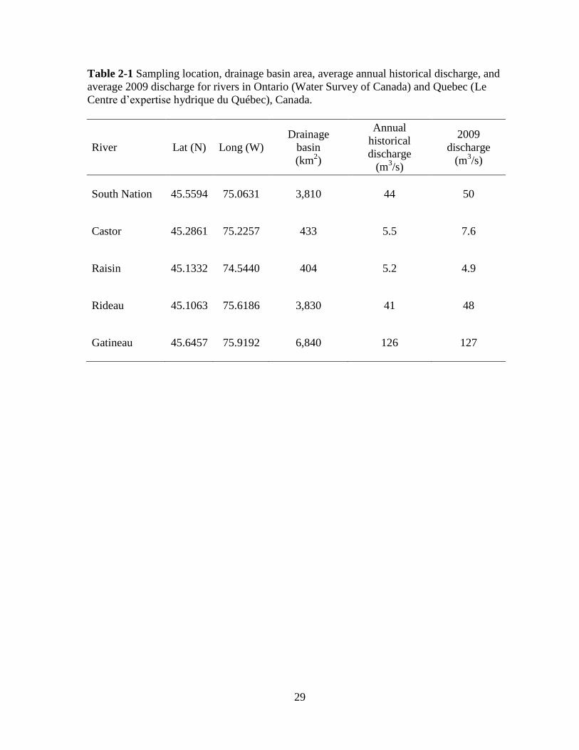
Table 2-1 Sampling location, drainage basin area, average annual historical discharge, and
average 2009 discharge for rivers in Ontario (Water Survey of Canada) and Quebec (Le
Centre d’expertise hydrique du Québec), Canada ................................................................... 29
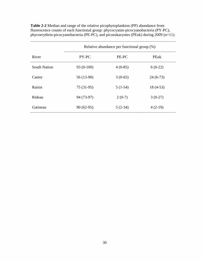
Table 2-2 Median and range of the relative picophytoplankton abundance from fluorescence
counts of each functional group: phycocyanin-picocyanobacteria (PY-PC), phycoerythrin-
picocyanobacteria (PE-PC), and picoeukaryotes (PEuk) during 2009 (n=11) ...................... .30
Table 2-3 Median and range of chlorophyll-a (Chl-a) and algal biomass based on
microscope enumerations during 2009 (n=8-11) .................................................................... 31
Table 2-4 Pearson correlations and statistical significance based on Bonferroni adjusted
probabilities (*p<0.05; ** p<0.01) for chlorophyll-a (chl-a) (n=47) and biomass based on
microscope enumerations (n=54) of the picophytoplankton size fraction (< 2 µm) and
phytoplankton greater than 2 µm in relation to environmental variables ............................... 32
Table 3-1 Regression analyses of slopes for phytoplankton size distribution based on chl-a
(log proportion of chl-a retained vs. log filter size) ................................................................ 51
Table 3-2 Summary of the size density regression analyses of log density vs. log GALD ... 52
Table 3-3 Bonferroni corrected Pearson correlation coefficients (*p<0.01) relating
phytoplankton density of different size classes to total phosphorus (TP, μg/L) and total
nitrogen (TN, μg/L) ................................................................................................................. 53
Table 4-1 Significant algal genera (≥ 15% of total biomass) in each river per sampling
period ....................................................................................................................................... 75
Table 4-2 Median and range of both biomass (mg/m3) and number of taxa per algal division
in each river (n=11) and the total per river (n=55) during the ice-free period of 2009 .......... 76
Table 4-3 Pearson correlations and statistical significance based on Bonferroni adjusted
probabilities (*p<0.05; ** p<0.01; *** p<0.001) for the following variables: pH, dissolved
oxygen percent saturation (% DO), temperature, conductivity (SPC), turbidity, water
discharge, reactive phosphorus (RP), total phosphorus (TP), ammonia+ammonium
(NH3+NH4+), nitrate (NO3
-), total nitrogen (TN), total chlorophyll-a (Chl-a) and total
biomass (mg/m3) for each main phytoplankton taxonomic divisions (n=55) ......................... 77
ix
List of Figures
Fig 2.1 Physical and chemical variables of rivers, 2009 ......................................................... 33
Fig 2.2 Picophytoplankton (PP) abundance separated by functional group: phycocyanin-rich
picocyanobacteria (PY-PC), phycoerythrin-rich picocyanobacteria (PE-PC), and
picoeukaryotes (PEuk) in the South Nation River (A-B), the Castor River (C-D), the Raisin
River (E-F), the Rideau River (G-H), and the Gatineau River (I-J) ....................................... 34
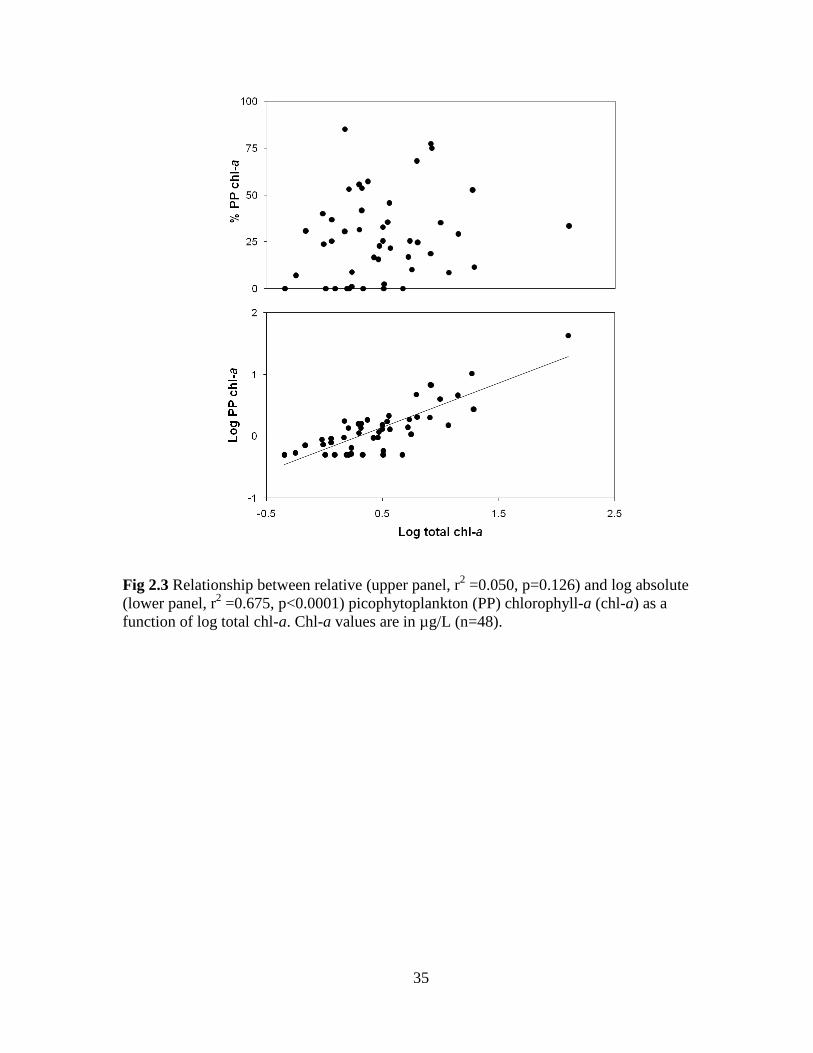
Fig 2.3 Relationship between relative (upper panel, r2 =0.050, p=0.126) and log absolute
(lower panel, r2 =0.675, p<0.0001) picophytoplankton (PP) chlorophyll-a (chl-a) as a
function of log total chl-a ........................................................................................................ 35
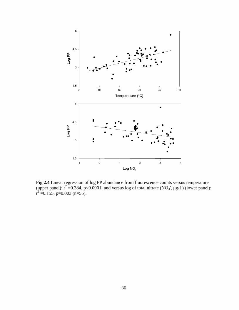
Fig 2.4 Linear regression of log PP abundance from fluorescence counts versus temperature
(upper panel): r2 =0.384, p<0.0001; and versus log of total nitrate (NO3
-, μg/L) (lower panel):
r2 =0.155, p=0.003 (n=55) ....................................................................................................... 36
Fig 3.1 The size distribution of chl-a from the proportion of total chl-a (μg/L) retained on the
filter and the log value of the filter size in the South Nation (A), the Castor (B), the Raisin
(C), the Rideau (D), and the Gatineau (E) rivers .................................................................... 54
Fig 3.2 Box plots of the relative phytoplankton chl-a in three size fractions (2-20, 20-64, and
> 64 µm) .................................................................................................................................. 55
Fig 3.3 The size-abundance spectra of each river (South Nation: 1-4; Castor: 5-8; Raisin; 9-
12; Rideau: 13-16; Gatineau: 17-20) presented as the log density of phytoplankton as a
function of the log mean greatest axial linear dimension (GALD) of each taxon per seasonal
category (spring, early summer, base flow, and fall) .............................................................. 56
Fig 3.4 Box plots of the density (cells/L) of phytoplankton in five size fractions:
picoplankton (< 2 µm), ultraplankton (2-10 µm), nanoplankton (10-20 µm), microplankton
(20-64 µm), and netplankton (> 64 µm) (upper panel), and per seasonal category: spring,
early summer, base flow, and fall (lower panel) ..................................................................... 57
Fig 3.5 The size distribution of chl-a (represented as the slope of relationships of Fig 3.1) in
relation to total phosphorus (upper panel; TP) and total nitrogen (lower panel; TN) ............. 58
Fig 3.6 The taxon-abundance spectra (represented as the slope of relationships of Fig 3.2) in
relation to total phosphorus (upper panel; TP) and total nitrogen (lower panel; TN) ............ 59
Fig 4.1 Percent phytoplankton biomass in major algal divisions throughout the study period
(May-November, 2009) in the Raisin River ........................................................................... 78
Fig 4.2 Percent phytoplankton biomass in the three most important algal divisions
throughout the study period (May-November, 2009) in the following rivers:
South Nation (A), Castor (B), Raisin (C), Rideau (D), Gatineau (E) ..................................... 79

- Chapter 1 -
Introduction
2
1.1 Introduction to river phytoplankton
Rivers are important freshwater resources for human use, and in addition harbour
significant biodiversity. In fact, many of the world’s great cities have been built along rivers.
However, over the last century, humans have caused extensive changes to the health of these
lotic ecosystems (e.g. Karr, 1999).
For rivers, as for other ecosystems, a healthy state has been defined as the system’s
ability to maintain structure and function against external stressors (Costanza and Mageau,
1999; Reynolds, 2003). For example, when the loading of organic wastes becomes excessive,
the assimilative capacity of the system is exceeded and the outcome can result in the loss of
fish habitat and the accumulation of undesirable taxa, such as toxic blooms of cyanobacteria
(blue-green algae) (Hötzel and Croome, 1994). Under these conditions, the stress and strain
exerted on the system leads to a loss of function (e.g. reductions in fish yields). Since rivers
are important ecosystems to maintain and manage, understanding their structure and function
is crucial. However, rivers, in comparison to lakes and oceans, have been studied far less,
particularly with respect to the ecology of primary producers (e.g. Rojo et al., 1994).
There are many different ways to assess the state of a river. Of these, the analysis of
benthic diatom communities has been successfully applied to assess water quality and
ecosystem health for several decades (Patrick, 1965). However, phytoplankton communities
have received much less attention, yet they are present in almost all major rivers that have
been studied (Greenberg, 1964; Lewis, 1988; Rojo et al., 1994; Train and Rodrigues, 1997)
and are present throughout the year (Sze, 1981).
Suspended algae in rivers can arise from several sources. Those that originate from
lakes are considered limnoplankton. Those that grow primarily on substrates but are then
entrained into the water column are in fact benthic algae, and true river phytoplankton that
3
grow in the river are termed potamoplankton (Reynolds, 2006). Early river research, such as
the River Continuum Concept (RCC), suggested that suspended algae were only abundant in
large rivers (Vannote et al., 1980); however, subsequent studies have demonstrated the
importance of phytoplankton in small to medium-sized temperate rivers (e.g. Søballe and
Kimmel, 1987; Basu and Pick 1996). More recent models of river systems suggest suspended
algae are important sources of carbon to river food webs (Thorp and Delong, 1994).
1.2 Factors influencing phytoplankton growth and seasonality
The ecological factors that influence phytoplankton growth in rivers are the same as
those regulating algal growth in lakes. These include light, nutrient concentrations, and
herbivore grazing. However, in rivers, water discharge (or flow) is a significant factor that
can constrain algal growth as advection downstream can lead to reductions in standing crop
(Søballe and Kimmel, 1987). Several studies have demonstrated water residence time as an
important factor for algal growth in lotic systems; longer water residence times tend to be
associated with increases in algal abundance (Søballe and Kimmel, 1987; Reynolds, 1988).
Light availability is an important variable regulating phytoplankton populations.
Throughout the growing season, the depth of the photic zone (depth of 1% of incident
radiation) varies in response to sediment loads in rivers and decreases when self-shading
occurs with high phytoplankton abundance. For example, in the Lot River in France, the
photic zone varies from 0.7 to 5.3 m throughout the year (Décamps et al., 1984). Generally,
when light becomes limiting, this leads to a reduction in phytoplankton abundance. For
example, in the highly turbid Ohio River, low light availability frequently limits
phytoplankton growth (Koch et al., 2004). The RCC considered light to be to be the most
important factor controlling autotrophic production in rivers (Vannote et al., 1980); however,
4
more recent studies have demonstrated the significant impact that nutrient concentrations
have on river phytoplankton (Søballe and Kimmel, 1987). For example, a study of 31 rivers
in eastern Canada reported a positive correlation between chlorophyll-a (chl-a) and total
phosphorus concentrations analogous to the well known relationship in lakes (Basu and Pick,
1996).
Both light and nutrients can be altered by the flow regime. Fast flowing water
increases turbulence and may affect light availability. In general, as rivers get deeper with
increasing flow, the mixed layer deepens such that suspended algae are entrained below the
euphotic zone. A ratio of euphotic zone to mixed layer depth less than 0.2 m is indicative of
light limitation and constrains phytoplankton growth (Cole et al., 1992). Changes in water
discharge caused by increased runoff (from precipitation, snow, or glacial melt) can also alter
transport and cycling of nutrients in the water column. In instances of high rainfall, nutrient
concentrations can rapidly increase or decrease several fold (e.g. Perkins and Jones, 1994).
There tends to be an inverse relationship between water discharge and river phytoplankton
abundance (Filardo and Dunstan, 1985; Sullivan et al., 2001). However, some taxa can
benefit from these conditions. For example, diatom abundance can increase in periods of
high rainfall and turbulence (Train and Rodrigues, 1997).
Grazing pressure can also play an important role in regulating phytoplankton
abundance. However, zooplankton grazing does not seem to significantly decrease algal
biomass in small to medium rivers (Pace et al., 1992; Reynolds and Descy, 1996). In
contrast, benthic grazers can considerably reduce phytoplankton populations (Basu and Pick,
1997; Caraco et al., 1997). For example, in the Hudson River (New York) the zebra mussel,
Dreissena polymorpha, was capable of filtering the entire water column every one to four
days in the summer. This decreased phytoplankton biomass by 85% and affected nutrient
5
concentrations, water clarity, and other variables at the ecosystem level (Caraco et al., 1997).
However, since grazing rates are normally low in medium to small rivers, the majority of the
primary production is usually carried downstream (Allan and Castillo, 2007).
Longitudinal and seasonal patterns are important to consider when assessing algal
communities in rivers. Significant changes in phytoplankton abundance can occur
longitudinally; early studies reported increases in phytoplankton abundance with downstream
travel (Greenburg, 1964; Hynes, 1970). In contrast, seasonal changes in phytoplankton
communities have not been as extensively studied (Hudon et al., 1996). There are no river
models of seasonal succession analogous to the Plankton Ecology Group-model that
describes the seasonal patterns and interactions of phytoplankton and zooplankton in
temperate lakes (Sommer et al., 1986).
The factors that regulate phytoplankton growth (nutrient concentrations, temperature,
light availability and discharge) vary seasonally in temperate rivers (Basu and Pick, 1997). In
the Rideau River (Ontario), a lowland mesotrophic system, nutrient concentrations are higher
in summer months (Basu and Pick, 1997). These coincide with increases in phytoplankton
abundance, seen as a positive relation between chl-a and TP (Basu and Pick, 1995 and 1997).
However, in the Ottawa River (Ontario), which is much larger and oligotrophic,
phytoplankton biomass varied little between spring, summer, and fall (Hudon et al., 1996),
although it tended to be highest during the low-discharge mid-summer period. In the
St. Johns River, Florida, fluctuating light availability influenced by seasonality strongly
affected phytoplankton abundance: less coloured water recorded in spring and summer led to
lower light extinction, thus favouring algal growth (Phlips et al., 2000).
6
1.3 Size distribution of phytoplankton
The size of an organism determines rate processes such as metabolism, production,
and excretion (White et al., 2007). Body size is also related to higher level attributes of
ecological systems such as population abundance, productivity, competitive and facilitative
relationships (Woodward et al., 2005). The relationship between body size and abundance
can determine resource allocation and shapes food web dynamics (Brown et al., 2004;
Woodward et al., 2005).
Body size analysis of phytoplankton communities is possible because individual taxa
range four orders of magnitude in size from small picoplankton (0.2-2 μm) to macroscopic
species with colonies visible to the naked eye (> 1000 μm) (Reynolds, 1984). The first
mention of phytoplankton distribution into size categories was in 1892 (Schütt, referenced in
Callieri, 2008). In the 1950s, screens, nets, and filters varying in pore size were used to
further separate plankton into size fractions. Upon the discovery of significant populations of
increasingly smaller phytoplankton cells, the following terms were introduced to describe
plankton size categories: micro-, nano-, ultra- and pico-plankton (Sicko-Goad and Stoermer,
1984).
Significant differences in size distribution can be observed in phytoplankton
communities because of the strong size dependence of growth rates, nutrient uptake, light
acquisition and sinking from the euphotic zone. Particularly in the oceans, the size
distribution of plankton has a major effect on biogeochemical cycles, in particular the carbon
cycle (Finkel et al., 2009).
The first examination of the size distribution or spectrum for plankton summarized
annual aggregations of the mean biomass of size classes of organisms in marine systems
(Sheldon et al., 1972). Since then, this approach has proven useful in marine systems
7
(Tremblay et al., 1997; Li, 2002) and in lakes (Sprules and Munawar, 1986). In marine
environments, positive correlations have been reported between average phytoplankton size
and chl-a (Li, 2002), nitrate (Vidal and Duarte, 2000), and iron (Tsuda et al., 2003)
concentrations. In lakes, phytoplankton average cell size tends to increase with nutrient
concentrations (Watson and Kalff, 1981). Generally, higher nutrient concentrations stimulate
phytoplankton growth and create a lag in the response of large predators to nutrient increases
(Armstrong, 2003). This creates more microzooplankton grazers that feed on the smaller
cells, thus favouring an increase in larger phytoplankton cell volume (Armstrong, 2003).
However, in shallow non-stratified lakes, small cells benefit from higher nutrient
concentrations (Reynolds, 1994). This occurs because they are more efficient at absorbing
light and have lower sinking rates and thus proliferate by remaining in the photic zone
(Reynolds, 1994; Finkel et al., 2009).
Few studies have investigated the link between size structure and nutrient
concentrations in rivers and streams (Rojo et al., 1994). One study of 46 temperate rivers
suggested that there was no significant variation in plankton size distribution conducted
during summer base flow conditions; nanoplankton (2-20 μm) dominated phytoplankton
biomass and no significant correlations were detected with nutrient concentrations (Chételat
et al., 2006). On the other hand, within one river (Rideau River), longitudinal differences
were observed where larger size classes (22-64 μm and > 64 μm fractions) consistently
increased in the downstream reaches from July to September. These patterns were
concomitant with longitudinal increases in nutrient concentrations and water residence times
(Yang et al., 1997).
In rivers, the different hydrological and hydrodynamic factors such as discharge and
water residence times may alter the phytoplankton community size structure (Chételat et al.,
8
2006). Because growth rate is inversely related to cell size (Reynolds, 1984), small cells in
theory should proliferate in river reaches and/or at times of short water residence times
whereas larger cells would be more abundant at longer water residence times. In the Rideau
River, increases in chl-a concentrations were found in reaches where water retention times
were 72 hours or longer (Basu and Pick, 1995). However, in rivers, phytoplankton
community size structure might be more affected by light availability than by the
hydrological regime because of high turbidity (Chételat et al., 2006). If light is limiting,
smaller cell sizes would be selected for because of how efficient they are at absorbing low
light (Reynolds, 1994).
1.4 Taxonomic composition of phytoplankton
Phytoplankton taxa present in rivers can reflect specific ecological conditions and
changes in species composition and distribution can be linked to the impact of pollution
(e.g. Giorgio et al., 1991). At highly impacted sites, broad-tolerance species may outcompete
more sensitive organisms and increase in abundance. For example, the presence of
planktonic diatom species such as Aulacoseira granulata, Stephanodiscus parvus, and
Stephanodiscus hantzschii indicate eutrophic conditions (Yang et al., 1997). With the
observation that certain species are abundant in specific environmental settings, the idea of
accessing river conditions based on community composition was developed. When changes
occur in species composition, this affects the functioning of the entire system (Karr, 1999).
Studying community species composition rather than the presence or absence of a particular
species is a more dependable way of assessing habitat conditions and several indices have
been developed to assess river conditions based on this knowledge (Karr, 1999; Reynolds
et al., 2002). In rivers, benthic diatoms are frequently used as bioindicators as they are
9
usually the most abundant type of algae and the composition of these communities is
particularly sensitive to environmental change (Kelly and Whitton, 1995). Recently, a biotic
index based on periphytic diatoms has been established for rivers in Canada (Lavoie et al.,
2008). These types of indices are based on the community composition of diatoms, which
reflect certain types of habitat and chemical conditions that indicate the overall state of the
river (e.g. Szczepocka and Szulc, 2009).
Most river studies have focused on diatoms and not the entire phytoplankton
community (Kelly, 1998; Fore and Grafe, 2002; Szczepocka and Szulc, 2009). In temperate
rivers, while diatoms appear to dominate in species abundance and biomass, the diversity of
river phytoplankton can be highly variable and other phytoplankton groups are also
important (Rojo et al., 1994). In a survey of 67 rivers, Rojo et al. (1994) found that diatoms
represented 40% of the average number of species in temperate rivers, yet green algae
contributed 28%, cyanobacteria represented 10%, and euglenoids averaged 7% of species
abundance. In a study of 31 temperate rivers in Ontario and Quebec, diatoms also dominated
with the largest percent of the total phytoplankton biomass (34%), however, other divisions
also contributed to overall biomass: cryptophytes (24%); chlorophytes and chrysophytes
(15%); and cyanobacteria (3%) (Chételat et al., 2006). Therefore, it is important to consider
other phytoplankton groups besides diatoms.
1.5 Thesis rationale and objectives
The overall objective of this thesis was to determine whether river phytoplankton can
be used to evaluate the state of rivers by analyzing communities over a growing season in
systems varying in physical and chemical conditions.
10
The first component of this research examined the contribution of the very smallest
phytoplankton to algal biomass. Picophytoplankton (0.2- 2 µm in diameter) have not been
well studied in rivers. Most studies describe phytoplankton in rivers without assessing
picophytoplankton because separate techniques are required to determine their abundance.
In Chapter 2, I hypothesized that picophytoplankton would not be significant in rivers
relative to larger phytoplankton. Since lake and ocean studies have demonstrated that these
small organisms are better competitors under low nutrient conditions (Stockner, 1988;
Søndergaard, 1991), I predicted that picophytoplankton abundance would only be significant
in the most oligotrophic rivers.
The second part of this thesis (Chapter 3) examined the use of phytoplankton size
distribution as an indicator of river condition, an approach which is widely used in marine
and lake ecosystems. The size distribution of chl-a and algal biomass from microscope
measurements were compared between seasons and rivers. I hypothesized that phytoplankton
size would differ mainly because of different nutrient concentrations such that higher
nutrient concentrations would lead to dominance of larger cells.
The last part of this research focused on the phytoplankton taxonomic community
composition of rivers (Chapter 4) and in particular the value of assessing all phytoplankton
taxa as opposed to only diatoms. The hypothesis that phytoplankton taxonomic composition
varies between rivers as a function of environmental variables was tested, and, in particular
that nutrient concentrations would be a significant driver of taxonomic composition.
- Chapter 2 -
Picophytoplankton in temperate rivers:
seasonal patterns and contribution to algal biomass
12
Abstract
Although picophytoplankton (0.2-2 µm) are ubiquitous in lake and oceans, their abundance
in rivers is considered insignificant to biomass and trophic dynamics. This study revisited
this assumption and examined picophytoplankton (PP) assemblages during the ice-free
period in five temperate rivers ranging in trophic state (9-107 µg/L total phosphorus). PP
abundance reached concentrations as high as those observed in lakes and oceans
(~ 104-10
5 cells/mL). For the most part, PP abundance was dominated by non-phycoerythrin
containing cyanobacteria; phycocyanin-rich cells accounted for approximately 75% of PP
abundance in all rivers. Multiple regression analysis determined that water temperature and
nitrate concentrations could explain about half of the variation in PP abundance across the
rivers (p<0.0001). The PP contribution to total chlorophyll-a averaged 27% (ranging 16-
46%) and did not decline with trophic state as in lakes. PP biomass from fluorescence
enumerations reached a maximum of 9% of total phytoplankton biomass, as high as observed
in lakes. The results of this study demonstrate the importance of including picophytoplankton
when analyzing phytoplankton communities in rivers.
13
2.1 Introduction
Phototrophic picoplankton (0.2-2.0 μm) were first discovered in the open ocean in the
late 1970s and subsequently in lakes in the early 1980s (Sieburth et al., 1978; Caron et al.,
1985). These pro- and eukaryotic cells account for 10-90% of biomass and/or production in
oceans and freshwater ecosystems and represent an important component of the microbial
food web (Stockner, 1991; Pick, 2000; Bell and Kalff, 2001). However, little is known about
these small cells in river systems. Photosynthetic picoplankton are considered insignificant in
rivers compared to lakes (Reynolds, 1994) and most studies of rivers have focused on larger
phytoplankton organisms such as nanoplankton and microplankton (e.g. Szelag-
Wasielewska, 2004; Szelag-Wasielewska et al., 2009).
Picophytoplankton (PP) are particularly important in terms of biomass and
productivity in oligotrophic systems as they have a high surface to volume ratio, which
provides a competitive advantage under low nutrient conditions (Raven, 1986; Søndergaard,
1991). When systems are nutrient enriched, larger cells tend to dominate (Watson and Kalff,
1981; Riegman et al., 1993). Several studies have shown that PP biomass and productivity
decreases in eutrophic lakes and oceans both empirically and experimentally (Perin et al.,
1996; Agawin et al., 2000; Pick 2000). However, recent studies have demonstrated higher
than expected PP biomass in eutrophic estuaries indicating that their abundance can also be
significant in nutrient-rich systems (Murrell and Lores, 2004; Gaulke et al., 2010). For
example, in North Carolina’s eutrophic Neuse River Estuary, PP (< 3 μm) contributed
between 35 and 44% of the total chlorophyll-a (chl-a) (Gaulke et al., 2010).
Studying PP abundance has proven useful for assessing environmental changes
because of their high growth rates (Stockner et al., 2000). PP respond rapidly to changing
environmental conditions and seasonality (Stockner et al., 2000; Wang et al., 2008). In lakes
14
and oceans, long water residence times coupled with warm temperatures represent
favourable conditions for high PP abundance (Phlips et al., 1999; Wakabayashi and Ichise,
2004). Seasonal distributions of PP communities show strong positive correlations with
temperature (e.g. Caron et al., 1985; Agawin et al., 2000). In Lake Ontario, the dominant
phycoerythrin picocyanobacteria peaked in abundance (6.5x10⁵ cells/mL) and biomass when
temperature was highest (Caron et al., 1985; Pick and Caron, 1987). Similarly, in an annual
study of phytoplankton communities along the salinity gradient of the York River in
Virginia, small cells (pico- and nanoplankton) were responsible for much of the chl-a in the
warmer summer months (Sin et al., 2000). Seasonality can also cause variations in
abundance for the different PP functional groups. A study of five oligotrophic to mesotrophic
lakes in Ontario showed that, while peaks of picocyanobacteria abundance occurred in
midsummer, the picoeukaryotic community represented on average about 50% of the
picoplankton biomass in spring and early summer (Pick and Agbeti, 1991).
Because of the challenges of taxonomically identifying cells at the limit of the light
microscope, PP have been classified into functional groups based on their photosynthetic
pigments. Two main groups can be distinguished by their fluorescence characteristics:
picocyanobacteria (PC) and picoeukaryote (PEuk) cell types. In freshwater systems there are
two main PC groups to consider: the first group contains phycocyanin (PY) phycobiliprotein,
whereas the other group contains phycoerythrin (PE) in addition to PY.
Phycoerythrin picocyanobacteria (PE-PC) tend to dominate oligotrophic to
mesotrophic systems while phycocyanin picocyanobacteria (PY-PC) are more dominant in
lakes with lower transparency resulting from either higher algal biomass or humic substances
(Pick, 1991). A parameterized competition model can be used to predict PC coexistence in
lakes and oceans; PE-PC tend to dominate in clear waters and PY-PC dominate in highly
15
turbid waters, while coexistence of both PC tend to occur at intermediate turbidity (Stomp
et al., 2007). Furthermore, lower light conditions in eutrophic systems seem to favour PEuk;
the contribution of PEuk to total PP appears to increase in more eutrophic lakes as a function
of increasing light attenuation (Craig, 1987; Pick and Agbeti, 1991). These findings suggest
niche differentiation of picophytoplankton along the light spectrum.
The goal of this study was to determine the ecological significance of PP in temperate
rivers. The first objective was to analyze seasonal variations of PP abundance and
composition based on the photosynthetic pigment groups (PY-PC, PE-PC, and PEuk). I
hypothesized that seasonal patterns are linked to changes in temperature such that increases
in water temperature would lead to increases in overall PP abundance, as observed in lakes.
The second goal was to compare PP in relation to the total algal community in rivers of
different trophic status along environmental gradients. I hypothesized that total PP
abundance in rivers is related to trophic state. Based on findings in lakes and oceans, I
expected that systems with lower nutrient levels would have higher overall PP abundance
than eutrophic rivers.
2.2 Methods
2.2.1 Study sites
Samples were collected from five temperate rivers in central Canada (Table 2-1). The
rivers chosen varied in nutrient concentrations because of different geology and land use
ranging from undisturbed forest to agricultural and urbanized areas. The most eutrophic
system, the South Nation River, is situated in a largely agricultural area where it rises near
the St. Lawrence River and flows in a north-easterly direction discharging into the Ottawa
River near Plantagenet, Ontario. The Castor River is a tributary of the South Nation River
16
and one of its four major sub-watersheds. The Raisin River is a low-land river that is also
mainly surrounded by agricultural lands, flowing into the St. Lawrence River near Lancaster,
Ontario, upstream of Montreal. Both the Castor and Raisin rivers have relatively low
discharge and are nutrient enriched (Basu and Pick, 1996). The Rideau River is a lake-fed
medium-size lowland river that flows from its headwaters, the Lower Rideau Lake, and
empties out into the Ottawa River (Basu and Pick, 1995). This mesoeutrophic system is
primarily used for recreation as part of the Rideau Canal system and is surrounded by
residential development as well as some agricultural lands. Lastly, the Gatineau River
represents the system least impacted by agriculture and urbanization and the most
oligotrophic (Basu and Pick, 1996). The Gatineau flows south from the Canadian Shield into
the Ottawa River. With the exception of the Raisin River, that discharges directly to the St.
Lawrence River, all rivers discharge to the Ottawa River.
All rivers sampled have gauging stations monitored by the Water Survey of Canada,
in Ontario and Le Centre d’expertise hydrique du Québec, in Quebec. Sites were chosen
upstream of these gauging station with no major tributaries in close proximity. These
gauging stations report the size of the upstream drainage basin as well as the historical and
daily river discharge (Table 2-1). For this study, discharge values were obtained by
calculating the average daily discharges seven days prior to and including the water
collection dates (Pace et al., 1992; Basu and Pick, 1996).
2.2.2 River sampling and laboratory analyses
Each river was sampled every two weeks from late May to early November 2009. On
occasion, sampling was postponed for a minimum of two days following major rain events.
A total of 11 samples were collected per river to describe the seasonal variability of the
17
water-column characteristics and algal abundance (Chételat and Pick, 2001). Water was
collected in Nalgene bottles mid-channel where rivers are typically deepest. The bottles were
triple rinsed with river water before collecting subsurface grab samples. In situ water
measurements of temperature, dissolved oxygen (DO), dissolved oxygen percent saturation
(%DO), pH, and conductivity (SPC) were taken with a Hydrolab Minisonde Multiprobe 4a.
Light measurements were occasionally taken using a LI-COR light meter and turbidity was
determined in the laboratory using a LaMotte 2020 turbidimeter following every sampling
event. Turbidity readings represent the ratio between the scattered light at 90 and 180
degrees from the light source and are given in Nephelometric Turbidity Units (NTU).
The water collected from each site was preserved in a 10% paraformaldehyde
solution in order to maintain, for approximately one month, the natural fluorescence of PP
(Stocker et al., 2000) and in Lugol’s iodine solution for phytoplankton identification. Water
samples were also brought to the City of Ottawa’s Robert O. Pickard Environmental Centre
for nutrient analysis using standard methods (Basu and Pick, 1995). The nutrients analyzed
were: total phosphorus (TP), reactive phosphorus (RP), total Kjeldahl nitrogen (TKN),
nitrate+nitrite (N03+N02), and ammonia+ammonium (NH3+NH4+). Total nitrogen (TN) was
calculated by adding TKN to N03+N02.
Because chl-a is widely used as a measure of phytoplankton biomass, chlorophyll
concentrations of the algal and PP communities were determined separately by parallel
filtration: individual 250 mL aliquots of water were filtered through 0.2 μm and 2 μm
polycarbonate membranes. When filtering the water, vacuum pressure was set below
15 mm Hg to avoid cell breakage. Following filtration, filters were stored at -25°C until they
were processed. Chl-a was extracted by adding 15 mL of ethanol to each sample for a
18
minimum of 24 hours, and concentrations were estimated with a Cary® 100 BIO UV-Visible
Spectrophotometer, Varian Inc (Jespersen and Christoffersen, 1987).
On the dates when analyses of the 2 μm fraction were taken in duplicate, the average
was calculated. For these duplicates, the coefficient of variation (CV) ranged from 7-21%
and averaged 14% across the rivers.
Chl-a collected on the 0.2 μm membranes represented total algal biomass while chl-a
collected on the 2 μm represented the biomass in the > 2 μm size fraction. PP chl-a (< 2 μm)
was calculated by subtracting the total chl-a from the greater than 2 μm chl-a. The
contribution of PP chl-a to total algal chl-a was expressed as a percentage of the total algal
chl-a.
2.2.3 Enumeration of phytoplankton
Fluorescence microscopy was used to quantify the abundance of PE-PC, PY-PC, and
of PEuk populations (Caron et al., 1985; Pick and Agbeti, 1991). From preserved samples,
an aliquot of 20 mL was vacuumed at low pressure (< 200 mm Hg) on Irgalan Black pre-
stained polycarbonate 0.2 μm membranes. Following filtration, the filters (~ 16-17 mm in
diameter) were placed on a microscope slide, followed by a drop of low fluorescence oil and
a glass cover placed over the filter. The microscope slides were then stored at -20 °C to
preserve the autofluorescence of cells until PP counts were processed.
The counts were made using a Zeiss AXIO A1 inverted microscope equipped with a
green excitation band pass (BP) of 546/12 nm and a red emission range of 575 nm to 640
nm. A second set of filters was used for blue excitation with a BP of 540-490 nm and an
emission long pass (LP) of 515 nm (yellow/orange emission). PY-PC were identified as red
fluorescing cells and enumerated using green excitation (Appendix 3) while the other cells
19
were counted using blue excitation. When excited with blue light, PE-PC appear as
yellow/orange cells and PEuk emission is red. Although PP have traditionally been counted
by epifluorescence microscopy (e.g. Pick and Caron, 1987), a fluorescence inverted
microscope is also suitable. Comparisons between the two methods yield similar results.
Enumerations were made for 30 randomly chosen fields of view for each cell type at
X1000 magnification. Cell counts included both rods and cocci type cells. Colonial forms of
PP assemblages were also counted; however, very few were seen in the river systems.
PP biomass (µg/L) based on enumerations was calculated by converting cell volume
(assuming a sphere with average radius of 0.5 μm) to biomass assuming a specific density of
1 g/cm3, used by convention for all phytoplankton taxa. Total algal biomass was calculated
from phytoplankton counts of cells greater than 2 μm using a Zeiss AXIO A1 inverted
microscope at X200, X400, and X630 magnifications. Ten mL of preserved phytoplankton
samples were settled overnight in 26 mm diameter chambers and enumeration of a minimum
of 300 cells per sample were made following the Utermöhl method (Lund et al., 1958).
Counts and cell dimensions were recorded using the computer counting program, Algamica,
version 4.0 (Gosselain and Hamilton, 2000). From this program, total volumetric biomass
(mg/m3) for cells > 2 μm were obtained for each sample. Total biomass was then calculated
by adding PP biomass to > 2 μm biomass values.
2.2.4 Data analysis
Statistical analyses consisted of parametric correlations and regressions. Bonferroni
adjusted Pearson correlations coefficients were calculated to determine the relationship
between physical and chemical variables and algal biomass from chl-a and microscope
counts for the PP and greater than 2 μm size fractions. Linear regressions were used to
20
determine the relationship between chl-a in < 2 μm size fraction and relative PP
concentrations from total chl-a. Multiple regression analyses, including forward and
backward procedures, were performed to provide the best model predicting PP abundance as
a function of environmental conditions. Variables were log transformed to satisfy normality
and all statistical analyses were done with S-Plus® version 8.0.
2.3 Results
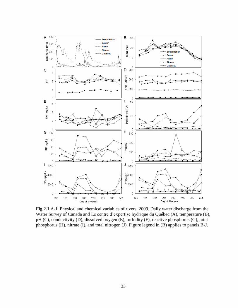
2.3.1 Physical and chemical variables
The largest river, the Gatineau River, had the highest annual average discharge
(127 m3/s) and the Raisin River had the lowest annual average discharge (4.9 m
3/s)
(Fig 2.1, A; Appendix 1). Water discharge varied seasonally with high discharge recorded
midsummer in 2009, mostly in July (Fig 2.1, A). High discharge values were also seen in late
fall, following many days of heavy rain. The South Nation and Castor rivers had the highest
turbidity values (Fig 2.1, F). Water clarity was lowest following periods of high water
discharge, as seen with the high turbidity reported in July and in the late fall.
Water temperature varied similarly in all rivers with low values recorded in late May
and in the fall, and high temperatures reported in the late summer months (Fig 2.1, B). A
maximum temperature of 28°C was recorded in the South Nation (June 24, 2009). Water pH
and conductivity varied the least seasonally, but had more pronounced differences between
rivers (Fig 2.1, C and D). The Gatineau River had the most neutral pH, while the other rivers
represented more alkaline conditions. Conductivity varied from as low as 20 µS/cm in the
Gatineau River to a maximum of 818 µS/cm in the Castor River. Dissolved oxygen (DO)
also varied throughout the season. The highest value, 14 mg/L (exceeding levels of saturation
at 170%), was recorded in the South Nation River (August 25, 2009).
21
The Castor, South Nation, and Raisin rivers had the highest nutrient concentrations
with the South Nation River being the most nutrient enriched (Fig 2.1, G to J). Seasonal
variations in reactive phosphorus (RP) concentrations were observed for each river, with
more pronounced differences observed in the South Nation River (Fig 2.1, G). The highest
total phosphorus (TP) concentration of the study was noted in the South Nation River on
August 25 (293 µg/L). The Rideau River had the second to lowest average annual
concentrations for TP (26 µg/L) and total nitrogen (TN, 712 µg/L) while the Gatineau River
had the lowest average TP (10 µg/L) and TN (376 µg/L) concentrations. Nitrate
concentrations varied similarly to TN throughout the study period in all rivers (Fig 2.1, I).
The average TN:TP ratio for all rivers was 33, indicating that phosphorus was more
likely to be limiting than nitrogen although the presence of significant levels of dissolved
inorganic nutrients suggest a lack of strong nutrient limitation overall. The Raisin River had
the lowest ratio (27), followed by the Rideau River, the South Nation River, the Castor
River, and the highest ratio (41) was observed in the Gatineau River.
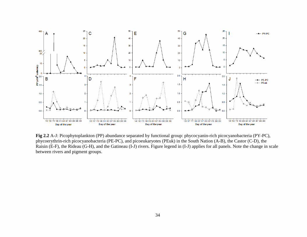
2.3.2 Seasonal patterns in density
Seasonal patterns of abundance for each pigment group of PP were observed in the
five rivers (Fig 2.2, A-J). The South Nation River showed the highest peak of PY-PC
abundance on June 24 (4.89x10⁵ cells/mL), the date and location where the highest water
temperature was also recorded, 28°C (Fig 2.2, A). A second, but less pronounced peak of
PY-PC was observed in early August. The PEuk community reached high density values in
late June and early July (~ 102-10
3 cells/mL). The PE-PC community showed consistently
low and essentially negligible abundance (Fig 2.2, B).
22
In the Castor River (Fig 2.2, C and D), the highest peak (2.07x10⁴ cells/mL) of PY-
PC occurred in early September. Although much lower in abundance, there were two peaks
noted for the PEuk community, in late June and early September. From May to November,
PE-PC contribution to PP abundance was also negligible. As in the Castor River, the highest
PP abundance recorded in the Raisin River occurred in early September (3.66x10⁴ PY-PC
cells/mL) (Fig 2.2, E). Two weeks prior and following that sampling event, the abundance of
PY-PC was also high compared to the other sampling dates. In addition as in the Castor,
PEuk abundance in the Raisin showed two peaks, the first in late June, and the second and
highest (3.24x10³ cells/mL) in early September. In comparison, the PE-PC community was
negligible, as found in both the South Nation and Castor (Fig 2.2, F).
In the mesoeutrophic Rideau River, PP seasonal abundance patterns were different
than those described in the more eutrophic systems (Fig 2.2, G and H). PY-PC abundance
was high throughout the summer months, except in early August, following a major rain
event. The highest abundance of PY-PC recorded was 4.54x10⁴ cells/mL in late August. For
the most part, the PEuk community was less abundant than PE-PC cells. Phycoerythrin-rich
PC reached higher densities than in the eutrophic rivers and showed a continuous increase in
abundance through the summer, leading to a maximum abundance in mid-September
(1.56x10³ cells/mL).
The Gatineau River had high abundances of PY-PC throughout the summer months
(Fig 2.2, I), with the highest recorded in mid-July (1.32x10⁴ cells/mL). PEuk and PE-PC had
similar seasonal abundance patterns with high density (~ 1.5x10³ cells/mL) in early summer
followed by continuous decreases in abundance (Fig 2.2, J).
For all the rivers, PY-PC was the most important PP pigment group (Table 2-2); on
average, 75% of total PP abundance corresponded to phycocyanin-rich PC while PEuk cells
23
contributed 13%, and approximately 11% was represented by PE-PC. The median relative
abundance of PE-PC was low for all rivers. However, on May 20, when phycocyanin-rich
cells were not present in the sample, PE-PC relative abundance in the South Nation River
was 85% (although their absolute abundance was very low at 2.25x10² cells/mL). PEuk were
relatively more important in the Castor and Raisin rivers with high contributions to total PP
density recorded in early July (73% and 53% respectively).
2.3.3 PP biomass from chl-a and microscope counts
Chl-a concentrations and biomass from microscope counts showed variations in the
distribution of phytoplankton biomass in the > 2 μm and < 2 μm size fractions within and
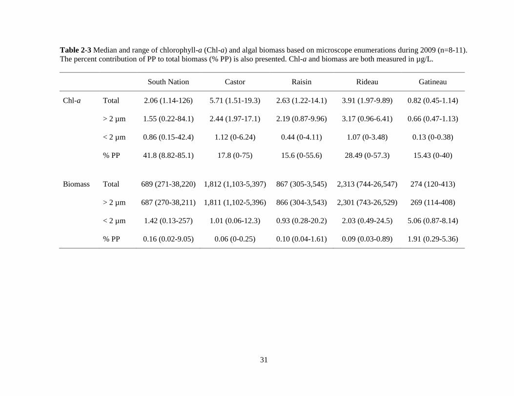
among the rivers (Table 2-3). The highest percent PP of total chl-a was recorded in the South
Nation River at 85% on June 5 and the highest relative PP biomass from microscope counts
was 9.05% on June 24 in the same river. On three separate sampling occasions in the South
Nation River the PP contribution to total chl-a was greater than 50%. The South Nation
River also had the highest total chl-a concentration on August 25 (126 μg/L) when the total
algal biomass, based on microscope counts, was also the highest (38,220 μg/L). Taxonomic
identification revealed that this high algal biomass was mostly caused by a bloom of the
colonial green alga, Pandorina morum (Appendix 6), but PP were also abundant (5.71x10³
cells/mL).
The Rideau River had the second highest relative contribution of PP to chl-a followed
by the Castor River, the Raisin River, and the Gatineau River (Table 2-3). For the total algal
chl-a concentrations, values were consistent with river trophic state as the most eutrophic
systems had the highest values and the most oligotrophic system, the Gatineau River, had the
lowest total median chl-a (0.82 μg/L).
24
Total algal biomass based on enumerations was also consistent with trophic state with
the exception of the South Nation River that had the second lowest median value (Table 2-3).
The relative contribution of PP to total biomass was much lower than the PP contribution to
total chl-a. The median relative contribution of PP to total algal biomass ranged from 0.06%
in the Castor River to 1.91% in the Gatineau River (Table 2-3).
Across rivers, the relative PP contribution to total chl-a showed no relationship with
chl-a (Fig 2.3, upper panel: r2= 0.050, p=0.126); whereas, the absolute PP chl-a showed a
statistically significant positive relationship with total chl-a biomass (Fig 2.3, lower panel:
r2= 0.675, p<0.0001).
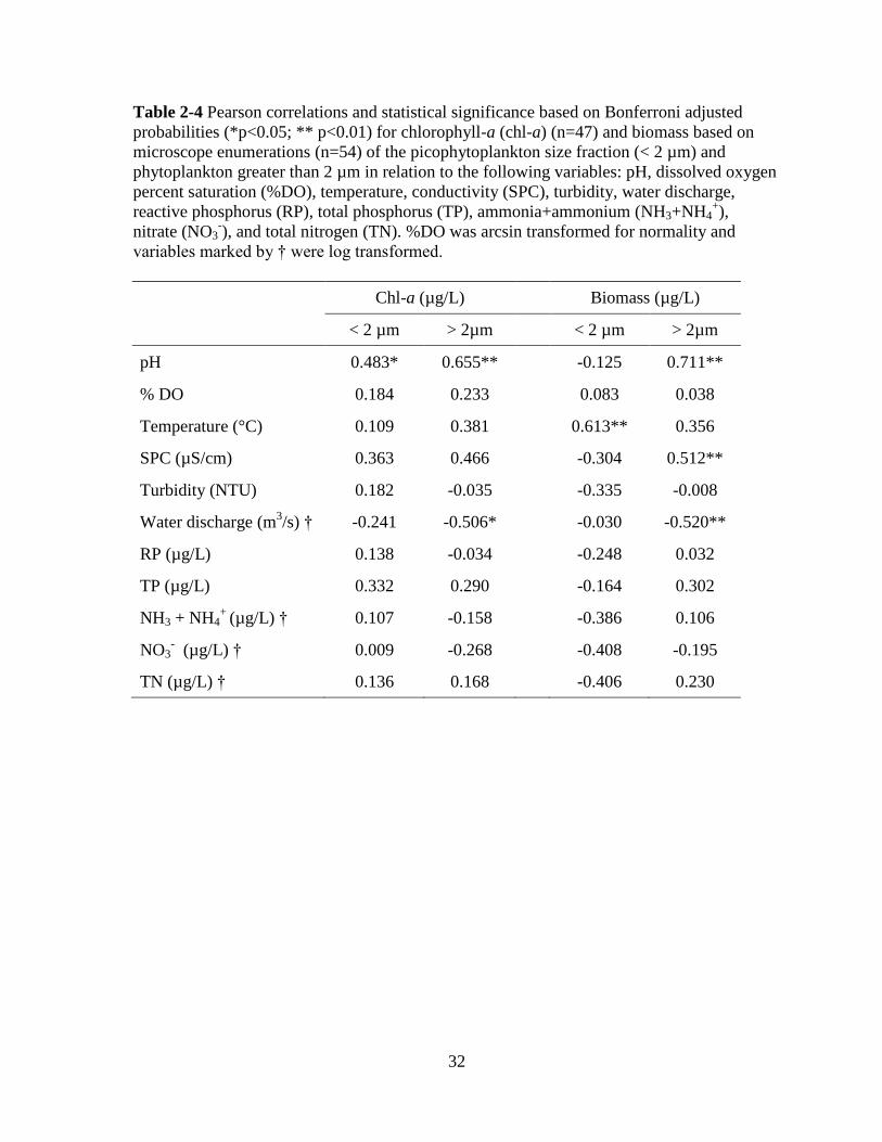
2.3.4 PP response to environmental variables
Chl-a concentrations and biomass from microscope counts in the pico fraction and in
the > 2 μm size class showed few statistically significant relationships with environmental
variables (Table 2-4). Positive correlations were associated with pH in both size fractions for
chl-a and in the > 2 μm for biomass based on biovolume. For the larger size fraction, the
only other statistically significant correlations were a negative response to water discharge
for both chl-a and biomass, and a positive response to SPC for the > 2 μm cells based on
microscope counts. The only statistically significant response of PP biomass from counts was
a positive correlation with temperature. For both the pico and larger cell sizes, no significant
response to nutrient concentrations was observed. TN and nitrate values were both negatively
correlated to PP biomass from microscope counts (~ r = 0.40), but due to the conservative
Bonferroni correction, the relationships were not statistically significant.
With respect to PP abundance, individual simple regressions indicated a positive
response to increasing water temperature (Fig 2.4, upper panel) and negative response to
25
nitrate concentrations (Fig 2.4, lower panel). Multiple regressions were used to evaluate the
response of PP abundance to the environmental variables measured concurrently (DO, pH,
temperature, conductivity (SPC), turbidity, discharge, RP, TP, nitrate, TN,
ammonia+ammonium, and extinction coefficient). Since DO is in part a product of algal
activity and is not likely controlling PP abundance, it was not included as an independent
variable. Light extinction was also excluded due to missing values. When multicollinearity
among the independent factors arose (based on results of a Pearson’s cross-correlation
analysis, Appendix 2), the most biologically significant variables were selected. For the
nutrients, because TP was highly correlated with RP, and TN with nitrate and ammonium,
the more bioavailable forms (i.e. RP and nitrate) were retained for the multiple regression
analysis. Furthermore, since turbidity and SPC were highly correlated to all nutrient
measurements and since pH was highly correlated to discharge, pH, turbidity, and SPC were
also excluded from the regressions. When temperature, discharge, RP, and nitrate were
considered in a multiple regression analysis, the variables that were retained and found to be
significant (whether using forward or backward stepwise regression analyses) were
temperature and nitrate. These two variables provided the best multiple regression model to
predict PP abundance and together explained 51% of the variation (p<0.0001) across rivers
(log (PP abundance) = 2.61 + 0.08 (Temperature) - 0.21 log (Nitrate)).
2.4 Discussion
In contrast to earlier assumptions from the literature (Reynolds, 1994), the results of
this study demonstrated that picophytoplankton can reach significant densities and are
important contributors to phytoplankton biomass in rivers ranging in trophic state. Densities
26
were as high as those reported from lakes and oceans (Partensky et al., 1996; Pick, 2000) and
ranged from 102 to 10
5 cells/mL.
Of the different pigments groups, phycocyanin-rich cyanobacteria dominated PP
abundance and comprised approximately three quarters of the total density. The strong
dominance of PY-PC type was anticipated given the empirical and experimental evidence
showing the numerical dominance of phycocyanin-rich picocyanobacteria in turbid waters
(Pick, 1991; Stomp et al., 2007). Collectively, the rivers in this study had a high average
light extinction coefficient (2.87/m) with values ranging from 0.70 to 6.9/m. The models of
Pick (1991) and Stomp et al. (2007) predict a decline in the PE-rich cyanobacteria and a rise
in the dominance (> 50%) of PY-cyanobacteria above extinction coefficients of 0.5/m. The
river results are also consistent with reports of PY-PC dominance in shallow eutrophic lakes
(Silvoso et al., 2010). PE-PC were not significant contributors to overall PP abundance
(~ 11%), but the highest average PE-PC abundance was found in the clearest river and more
oligotrophic rivers, the Gatineau and the Rideau rivers. PEuk were more abundant in early
summer and sometimes had two peaks in abundance, one in early summer and the other
occurring late August. Similar patterns have been described in lakes where PEuk were
generally one order of magnitude less abundant than PC and often showed peaks in spring
and midsummer (Pick and Agbeti, 1991; Stockner, 1991; Callieri and Stockner, 2002).
In the rivers of this study, the contribution of PP to total chl-a and biomass was
significant (~ 27% on average) but was not a simple function of river trophic state
(Table 2-3, Fig 2.2). In contrast, in lakes, the percent contribution of PP to total biomass
clearly decreases with increasing trophic status (Søndergaard et al., 1991, Vörös et al., 1998;
Callieri et al., 2007). In this study, even in the most eutrophic system (i.e. South Nation
River), PP still contributed to almost half of the total chl-a. These findings are consistent
27
with a recent study reporting a high contribution of PP to total planktonic chlorophyll in a
eutrophic estuary (Gaulke et al., 2010). PP biomass from microscope counts also accounted
for as much as 9% of total biomass, which is consistent with estimates from Ontario lakes
(Pick and Abgeti, 1991).
The most important factor explaining variation in PP abundance was temperature. In
this study, high abundance of PP was linked to high temperatures, observed throughout the
summer months similarly across the rivers. This is consistent with previous studies linking
high PP biomass with optimal temperatures above 20°C (Agawin et al., 2000; Gaulke et al.,
2010). In Lake Maggiore, maximal PP abundances were noted when surface water reached
18°C to 20°C (Callieri and Piscia, 2002). Similarly, in a study of five oligotrophic to
mesotrophic Ontario Lakes, PC abundance was highest in the late summer months when
temperature was greater than 20°C (Pick and Agbeti, 1991). In this study, the highest PP
abundance (4.89x10⁵ cells/mL) occurred on the same day as the highest water temperature
was recorded (28°C) in the most eutrophic and turbid river (South Nation).
PP abundance was not related to river discharge, in contrast to the significant
negative relationship observed between larger phytoplankton and discharge for both chl-a
and biomass from enumerations (Table 2.4). This is likely because the growth rates of PP are
very fast (doubling times < 1- 2 days, Lavallée and Pick, 2002), particularly at higher
temperatures, such that losses from advection downstream are insignificant. Several river
studies have reported negative relationships between algal biomass and discharge (Reynolds,
1984) because relatively long water residence times may be required to enable accumulation
of slower growing algae (i.e. larger taxa).
PP abundance was also not positively related to nutrient concentrations, as might be
expected if nutrients were limiting this community. However, PP are likely rarely nutrient
28
limited in rivers given their high affinity for nutrients at low concentrations and the generally
higher nutrient supply rates. In the more eutrophic rivers, reactive phosphorus was above
detection and at times quite high, which is indicative of a surplus of bioavailable phosphorus.
Interestingly enough, PP abundance exhibited a negative relationship with nitrate. This could
reflect either strong consumption of nitrate or competition for nitrate with large
phytoplankton or some indirect effect of top down factors operating in the more eutrophic
rivers. Negative effects of nutrients on PP have been demonstrated experimentally in lakes
(Tzaras et al., 1999). While the larger phytoplankton biomass was not correlated with
nutrients (phosphorus and nitrogen fraction), a significant correlation with conductivity was
observed and conductivity has been considered a surrogate of productivity in rivers (Biggs,
1988). However, large phytoplankton in this river study were highly sensitive to discharge;
this is in contrast to broader regional studies and larger data sets that suggest that nutrients
are the primary factor controlling algal biomass in rivers as in lakes (Basu and Pick, 1996;
Van Nieuwenhuyse and Jones, 1996).
In summary, this study demonstrated the importance of picophytoplankton to the
plankton of temperate rivers, regardless of trophic state and river size. Given their high
turnover rates, the community also likely plays an important role in river carbon and nutrient
cycling that has yet to be recognized.
29
Table 2-1 Sampling location, drainage basin area, average annual historical discharge, and
average 2009 discharge for rivers in Ontario (Water Survey of Canada) and Quebec (Le
Centre d’expertise hydrique du Québec), Canada.
River Lat (N) Long (W)
Drainage
basin
(km2)
Annual
historical
discharge
(m3/s)
2009
discharge
(m3/s)
South Nation 45.5594 75.0631 3,810 44 50
Castor 45.2861 75.2257 433 5.5 7.6
Raisin 45.1332 74.5440 404 5.2 4.9
Rideau 45.1063 75.6186 3,830 41 48
Gatineau 45.6457 75.9192 6,840 126 127
30
Table 2-2 Median and range of the relative picophytoplankton (PP) abundance from
fluorescence counts of each functional group: phycocyanin-picocyanobacteria (PY-PC),
phycoerythrin-picocyanobacteria (PE-PC), and picoeukaryotes (PEuk) during 2009 (n=11).
Relative abundance per functional group (%)
River PY-PC PE-PC PEuk
South Nation 93 (0-100) 4 (0-85) 6 (0-22)
Castor 56 (13-90) 3 (0-65) 24 (6-73)
Raisin 75 (31-95) 5 (1-54) 18 (4-53)
Rideau 94 (73-97) 2 (0-7) 3 (0-27)
Gatineau 90 (62-95) 5 (2-34) 4 (2-19)
31
Table 2-3 Median and range of chlorophyll-a (Chl-a) and algal biomass based on microscope enumerations during 2009 (n=8-11).
The percent contribution of PP to total biomass (% PP) is also presented. Chl-a and biomass are both measured in µg/L.
South Nation Castor Raisin Rideau Gatineau
Chl-a Total 2.06 (1.14-126) 5.71 (1.51-19.3) 2.63 (1.22-14.1) 3.91 (1.97-9.89) 0.82 (0.45-1.14)
> 2 µm 1.55 (0.22-84.1) 2.44 (1.97-17.1) 2.19 (0.87-9.96) 3.17 (0.96-6.41) 0.66 (0.47-1.13)
< 2 µm 0.86 (0.15-42.4) 1.12 (0-6.24) 0.44 (0-4.11) 1.07 (0-3.48) 0.13 (0-0.38)
% PP 41.8 (8.82-85.1) 17.8 (0-75) 15.6 (0-55.6) 28.49 (0-57.3) 15.43 (0-40)
Biomass Total 689 (271-38,220) 1,812 (1,103-5,397) 867 (305-3,545) 2,313 (744-26,547) 274 (120-413)
> 2 µm 687 (270-38,211) 1,811 (1,102-5,396) 866 (304-3,543) 2,301 (743-26,529) 269 (114-408)
< 2 µm 1.42 (0.13-257) 1.01 (0.06-12.3) 0.93 (0.28-20.2) 2.03 (0.49-24.5) 5.06 (0.87-8.14)
% PP 0.16 (0.02-9.05) 0.06 (0-0.25) 0.10 (0.04-1.61) 0.09 (0.03-0.89) 1.91 (0.29-5.36)
32
Table 2-4 Pearson correlations and statistical significance based on Bonferroni adjusted
probabilities (*p<0.05; ** p<0.01) for chlorophyll-a (chl-a) (n=47) and biomass based on
microscope enumerations (n=54) of the picophytoplankton size fraction (< 2 µm) and
phytoplankton greater than 2 µm in relation to the following variables: pH, dissolved oxygen
percent saturation (%DO), temperature, conductivity (SPC), turbidity, water discharge,
reactive phosphorus (RP), total phosphorus (TP), ammonia+ammonium (NH3+NH4+),
nitrate (NO3-), and total nitrogen (TN). %DO was arcsin transformed for normality and
variables marked by † were log transformed.
Chl-a (µg/L)
Biomass (µg/L)
< 2 µm > 2µm
< 2 µm > 2µm
pH 0.483* 0.655**
-0.125 0.711**
% DO 0.184 0.233
0.083 0.038
Temperature (°C) 0.109 0.381
0.613** 0.356
SPC (µS/cm) 0.363 0.466
-0.304 0.512**
Turbidity (NTU) 0.182 -0.035
-0.335 -0.008
Water discharge (m3/s) † -0.241 -0.506*
-0.030 -0.520**
RP (µg/L) 0.138 -0.034
-0.248 0.032
TP (µg/L) 0.332 0.290
-0.164 0.302
NH3 + NH4+
(µg/L) † 0.107 -0.158
-0.386 0.106
NO3- (µg/L) † 0.009 -0.268
-0.408 -0.195
TN (µg/L) † 0.136 0.168
-0.406 0.230
33
Fig 2.1 A-J: Physical and chemical variables of rivers, 2009. Daily water discharge from the
Water Survey of Canada and Le centre d’expertise hydrique du Québec (A), temperature (B),
pH (C), conductivity (D), dissolved oxygen (E), turbidity (F), reactive phosphorus (G), total
phosphorus (H), nitrate (I), and total nitrogen (J). Figure legend in (B) applies to panels B-J.
34
Fig 2.2 A-J: Picophytoplankton (PP) abundance separated by functional group: phycocyanin-rich picocyanobacteria (PY-PC),
phycoerythrin-rich picocyanobacteria (PE-PC), and picoeukaryotes (PEuk) in the South Nation (A-B), the Castor (C-D), the
Raisin (E-F), the Rideau (G-H), and the Gatineau (I-J) rivers. Figure legend in (I-J) applies for all panels. Note the change in scale
between rivers and pigment groups.
35
Fig 2.3 Relationship between relative (upper panel, r2 =0.050, p=0.126) and log absolute
(lower panel, r2 =0.675, p<0.0001) picophytoplankton (PP) chlorophyll-a (chl-a) as a
function of log total chl-a. Chl-a values are in µg/L (n=48).
36
Fig 2.4 Linear regression of log PP abundance from fluorescence counts versus temperature
(upper panel): r2 =0.384, p<0.0001; and versus log of total nitrate (NO3
-, μg/L) (lower panel):
r2 =0.155, p=0.003 (n=55).
- Chapter 3 -
The influence of season and trophic state on
phytoplankton size distribution in temperate rivers
38
Abstract
The size structure of communities has been used as an alternative to taxonomic analyses to
assess anthropogenic stresses in aquatic environments. This study examined phytoplankton
size distribution using two methods in five temperate rivers ranging in trophic state
throughout the ice-free season. Seasons were separated into four categories: spring, early
summer, base flow, and fall. The size distribution of suspended chl-a was analyzed by linear
regression as the proportion of chl-a retained on the filter versus filter size. Taxon-abundance
spectra were analyzed by linear regression as phytoplankton density vs. the mean greatest
axial linear dimension (GALD) of each taxon in the sample. The regression slopes for these
analyses were used as a measure of change in the relative importance of small versus large
cells. There was no significant effect of river or season on the slopes of both estimates of size
distribution. However, the slopes of the suspended chl-a size distribution were positively
correlated with total nitrogen (TN) concentrations, but the latter only explained 20% of the
variance. Slopes for the taxon-abundance size spectra did not significantly vary with TN
concentrations and neither size distribution was related to total phosphorus (TP)
concentrations. The microplankton (20-64 µm) was the only size fraction to significantly
respond to nutrients. The results of the study demonstrate the stability of the phytoplankton
size distribution slopes across different rivers throughout the ice-free period and the lack of
response to changing nutrient concentrations. The phytoplankton size distribution in
temperate rivers appears relatively invariant and is thus not a useful indicator of river
condition.
39
3.1 Introduction
In aquatic ecosystems, body size distributions have been used as a measure of
community structure instead of taxonomic based descriptions (Cattaneo et al., 1997;
DeNicola et al., 2006; Finkel et al., 2009). This approach is particularly useful when
analyzing planktonic communities since many small taxa are difficult to identify or remain
unknown. Body size drives fundamental rate processes (e.g. metabolism, grazing, and
sedimentation) that collectively affect ecosystem functions. Sheldon et al. (1972) was the
first to describe a biomass distribution model of marine plankton communities and noted that
the biomass found in logarithmically equal size intervals was roughly constant. Since
Sheldon et al. (1972), studies have demonstrated the ecological significance and
predictability of size biomass or abundance models in aquatic systems (Sprules et al., 1983;
Sprules and Munawar, 1986). Changes in cell size distribution can be used to provide early
indications of stressors such as nutrient enrichment (Sprules and Munawar, 1986;
Wunsam et al., 2002). However, in rivers, few studies have assessed phytoplankton size
distribution (Rojo et al., 1994; Chételat et al., 2006).
Factors such as nutrients, temperature, and light can influence body size distribution
in lakes and oceans (Cyr et al., 1997). In general, algal biomass is usually controlled by
nutrient concentrations but shifts in phytoplankton size distribution with nutrient enrichment
can also occur because of different taxon size resource requirements or grazing pressure
(Malone, 1980; Vanni, 1987). When nutrients are limiting, small cells often dominate larger
cells because their high surface area to volume ratio makes them better at acquiring nutrients
(Wen et al., 1997). In lakes, nanoplankton often dominate oligotrophic systems, while larger
cells are more abundant in eutrophic environments (Watson and Kalff, 1981; Kalff, 2002).
However, studies of diatom size distribution have reported variables results. For example, a
40
study of intermediate-sized alkaline lakes reported negative responses of planktonic diatom
cell size with increasing phosphorus and nitrogen concentrations (Finkel et al., 2009).
Similar patterns have been observed for benthic algae in lakes and streams: in situ
and experimental studies have demonstrated a positive response of periphyton cell size to
increasing phosphorus concentrations in these systems (Cattaneo, 1987; Cattaneo et al.,
1997; DeNicola et al., 2006). In Quebec streams, Lavoie et al. (2006, 2010) demonstrated
that benthic diatom size distributions did not respond to environmental change, in particular
phosphorus concentrations, and concluded that diatom body size should not be used as a
proxy for nutrient status in environmental monitoring.
Trends observed in lakes might differ for rivers due to the physical differences related
to discharge and light availability between the two types of ecosystems. In rivers, discharge
may impact cell size distributions as longer residence times might allow for larger cells to
increase their biomass. In a mesoeutrophic river, the Rideau River (Ontario), larger size
classes (20-64 µm and > 64 µm) were observed more frequently in downstream reaches
where water residence times were longer (Yang et al., 1997). In rivers, the presence of
suspended materials, combined with the lack of stratification, can lead to highly turbid
environments. Under light limiting conditions, small cells are favoured since they can out-
compete larger cells due to their greater light capturing abilities (Cole et al., 1992). This was
observed in a study of 46 rivers in Ontario and western Quebec where the smallest cells, the
nanoplankton (2-20 µm), dominated biomass (Chételat et al., 2006). In temperate rivers,
light limiting conditions would be more pronounced during periods of high flow such as the
spring.
The goal of this study was to determine if phytoplankton size distribution can be used
as an alternative method to taxonomic resolution when assessing the state of rivers. Since
41
previous studies have focused on slope analyses of size distributions (or size spectra)
(Shin et al., 2005, Petchey and Belgrano, 2010), I examined seasonal patterns of the slopes
of both phytoplankton abundance and biomass versus cell size among different rivers
ranging in physical and chemical conditions. I hypothesized that phytoplankton size
distribution patterns are linked to trophy such that increases in nutrient concentrations would
lead to the dominance of larger cell sizes. As found in lakes, smaller cells were expected to
dominate under more oligotrophic conditions.
3.2 Methods
3.2.1 Study sites
Samples were collected from five temperate Ontario and Quebec rivers ranging in
land use and nutrient concentrations. River descriptions and hydrological regimes are
summarized in Chapter 2 (Table 2-1).
3.2.2 River sampling and laboratory analyses
Each river was sampled every two weeks from late May until early November 2009.
On occasion, sampling was postponed for a minimum of two days following major rain
events. A total of 11 samples were collected per river to represent phytoplankton
communities and river conditions over the growing season (Chételat and Pick, 2001). Water
was collected in Nalgene bottles mid-channel where rivers are typically deepest. The bottles
were triple rinsed with river water before collecting subsurface grab samples. In situ water
measurements of temperature, dissolved oxygen (DO), dissolved oxygen percent saturation
(%DO), pH, and conductivity (SPC) were taken with a Hydrolab Minisonde Multiprobe 4a.
Light measurements were occasionally taken using a LI-COR light meter and turbidity was
42
determined in the laboratory using a LaMotte 2020 turbidimeter following every sampling
event. Turbidity is a measure of the degree of light scattering, related to particle
concentration.
The water collected from each site was preserved in a 10% paraformaldehyde
solution in order to maintain, for approximately one month, the naturally occurring
fluorescence in picophytoplankton (Stocker et al., 2000) and in Lugol’s iodine solution for
phytoplankton (> 2 µm) identification. Water samples were also brought to the City of
Ottawa’s Robert O. Pickard Environmental Centre for nutrient analysis using standard
methods (Basu and Pick, 1995). The nutrients analyzed were: total phosphorus (TP), reactive
phosphorus (RP), total Kjeldahl nitrogen (TKN), nitrate+nitrite (N03+N02), and
ammonia+ammonium (NH3+NH4+). Total nitrogen (TN) was calculated by adding TKN to
N03+N02.
3.2.3 Phytoplankton chl-a fractions and microscope enumerations
Chlorophyll-a (chl-a) concentrations in different size fractions were determined by
parallel filtration the same day sampling occurred. Separate aliquots of water were filtered
through 0.2 μm, 2 μm, 10 μm and 20 μm polycarbonate filters, whereas 35 μm and 64 μm
were filtered through Nitex mesh. For the 0.2 μm and 2 μm filters, 250 mL of water was used
whereas 500 mL was filtered through the larger pore size filters. A separate aliquot of
500 mL of water was also filtered through glass microfiber Whatman 934-AH 47 mm filters
(~ 1.5 μm pore size). When filtering the water, the vacuum pressure was set below
15 mm Hg to avoid cell breakage. The polycarbonate membranes for the small pore sizes
came from different providers (GE Polycarbonate from Water & Process Technologies for
the 0.2 μm and 10 μm filters, and Poretics for the 2 μm and 20 μm filters).
43
Following filtration, filters were stored at -25°C until they were processed. Chl-a
was extracted by adding 15 mL of ethanol to each sample for a minimum of 24 hours, and
concentrations were estimated with a Cary® 100 BIO UV-Visible Spectrophotometer,
Varian Inc (Jespersen and Christoffersen, 1987). The 0.2 μm and 10 μm filters were less
resistant to more aggressive solvents such as DMSO therefore ethanol was used to extract
chl-a (Burnison, 1980; Jespersen and Christoffersen, 1987) from all filters. On the dates
when analyses of the 2 μm and 10 μm fractions were taken in duplicate, the average and the
coefficient of variation (CV) were calculated. Across rivers, the CV of the 2 μm filters
averaged 14% (range 7-21%) and 11% for the 10 μm filters (range 6-15%).
Phytoplankton identification and enumerations were made using a Zeiss AXIO A1
inverted microscope. Picophytoplankton (0.2-2 μm) counts were made for 30 randomly
chosen fields of view at X1000 magnification under fluorescence (Chapter 2). An aliquot of
20 mL was vacuumed at low pressure (< 200 mm Hg) on Irgalan Black pre-stained
polycarbonate 0.2 μm membranes. Phytoplankton greater than 2 μm preserved in Lugol’s
were counted and measured under light microscopy at X200, X400, and X630
magnifications. Ten mL of Lugol’s preserved water samples were settled overnight in 26 mm
diameter chambers and the enumeration of a minimum of 300 cells per sample were made
following the Utermöhl method (Lund et al., 1958). Counts and cell dimensions were
recorded using the computer counting program, Algamica, version 4.0 (Gosselain and
Hamilton, 2000). Algamica calculates cell density and the mean greatest axial linear
dimension (GALD) based on dimensions measured for each taxon per sample. The program
also computes total density for the following size fractions: picoplankton (< 2 µm),
ultraplankton (2-10 µm), nanoplankton (10-20 µm), microplankton (20-64 µm), and
44
netplankton ( > 64 µm). Picophytoplankton abundance from fluorescence counts were added
to the light microscope counts using a GALD of 1 µm.
3.2.4 Data analysis
Seasonal data were pooled into four time periods: spring, early summer, base flow,
and fall. Spring was based on three sampling occurrences from late May until end of June,
representing the period of declining discharge. The early summer category consisted of three
sampling dates covering July to early August. Since during 2009 heavy rain was recorded
throughout the month of July, base flow conditions occurred later during the ice-free season;
late August and September (n=3) represented base flow conditions. Fall samples were
represented by two sampling dates that took place in October and early November when the
flows tend to rise again.
The relationship between the proportion of chl-a retained on the filter and filter size
was used to describe the size distribution of suspended chl-a for each river according to
season. The slope of this relationship was then used to quantify in one metric the relative
importance of small versus large cells. This approach is similar to the one used by Mazumder
et al. (1988) to examine the size distribution of particulate phosphorus in aquatic systems.
The slopes of the relationship between phytoplankton density and the GALD of each taxon
across the rivers and seasons were also analyzed, and included all phytoplankton taxa. This is
similar to mass density analyses developed for other taxonomic groups (e.g. Currie and Fritz,
1993) and relates to metabolic scaling, an active area of research in ecology (e.g. White
et al., 2007).
Statistical analyses consisted of correlations, regressions, and analysis of variance
(ANOVA). Pearson correlation analysis was used to determine the response of
45
phytoplankton density separated into size fractions to TP and TN. Linear regressions were
used for the analysis of the size distribution (slope data) of suspended chl-a and taxon-
abundance, and to determine the relationship between size distribution and environmental
variables. Two-way ANOVAs were carried out to determine the effect of river and season on
the phytoplankton size distributions based on chl-a and taxonomic enumerations. One-way
ANOVAs were used to determine the effect of different size fractions and the effect of
seasonal periods on phytoplankton biomass from chl-a and density. For these analyses, the
assumption of normality, homoscedasticity, and independence were tested using the residuals
and statistical significance was considered when p<0.05. All statistical analyses were done
with S-Plus® version 8.0; certain variables required log transformations to satisfy normality.
3.3 Results
3.3.1 Physical and chemical variables
Physical and chemical parameters varied throughout the study period and across the
different rivers. A summary of these variables can be found in Chapter 2 (Fig 2.1,
Appendix 1).
3.3.2 Size distribution of suspended chl-a
The size distribution of suspended chl-a was examined across the five rivers and
seasons (Fig 3.1 and Table 3-1). The relationships between filter size and the proportion of
chl-a observed in size fractions ranging from picoplankton to net plankton were all strong
and highly significant (r2 > 0.80, p<0.05). The regression slopes ranged from -0.683 to
-0.284: more negative slopes mean a greater proportion or dominance of small cells vs. large
cells. The average slope was -0.455 and ranged from an average of -0.504 in the Gatineau to
46
-0.417 in the South Nation. Seasonally, the shallowest slope was observed in the Castor
during spring (-0.284) and the steepest slope in the Gatineau during fall (-0.683). However,
overall there was no significant effect of river or season on the slopes of the size distribution
of chl-a and there were no significant interactions (two-way ANOVA, p>0.05).
A one-way ANOVA determined a significant difference between relative chl-a
biomass in three size fractions (p<0.05) (Fig 3.2). On average, the smallest size fraction
(2-20 μm) accounted for almost two-thirds of total biomass, cells between 20 and 64 μm
represented 32% of biomass, and the largest cells (> 64 μm) contained the least biomass
(4%). The dominance of small cells was consistent throughout the study period.
3.3.3 Phytoplankton density size distribution
Phytoplankton taxon abundance in relation to the GALD of each taxon was also
analyzed seasonally within and between the rivers (Fig 3.3 and Table 3-2). GALD generally
explained less than half of the variance (r2
≈ 0.40) in phytoplankton density, but all
relationships were significant, with the exception of two sampling dates. The average
regression slope was -1.061 and ranged from an average of -1.168 in the Rideau to an
average of -0.967 in the Gatineau. The South Nation had the steepest individual slope in
spring time (-1.941) and the Raisin the shallowest individual slope (-0.495) in early summer
(Table 3-2). Overall, the steepest slopes tended to be associated with the base flow period
(-1.179) and the shallowest in the fall (-0.911). However, as for the chl-a size distributions,
there were no significant effects of river and season on the taxon-abundance spectra (two-
way ANOVA, p>0.05) and no interactions detected.
Phytoplankton density differed significantly among the five size fractions and with
respect to season (one-way ANOVA, p<0.05) (Fig 3.4). As expected, the picoplankton size
47
fraction had the highest median density (3.42x10⁶ cells/L), followed by the ultraplankton,
nanoplankton, and microplankton. The least abundant size fraction was netplankton with a
median density of 1.63x10⁴ cells/L. Across seasons, base flow had the highest median
density (1.41x10⁷ cells/L) and this was statistically different (t-test; p<0.05) than the lowest
median density observed in the fall (2.03x10⁶ cells/L).
3.3.4 Nutrients and phytoplankton cell size
There was no relationship between the slopes of the size distribution of suspended
chl-a and TP (r2 =0.061, p=0.071) but there was a significant positive relationship with TN
(r2 =0.196, p<0.001) (Fig 3.5). The chl-a based slopes were less steep in samples with higher
TN indicating that larger taxa were more important under higher nitrogen concentrations. No
statistically significant relationships between the slopes of the size-abundance spectra from
density vs. GALD measurements (Fig 3.6) were observed between TP concentrations
(r2 =0.005, p=0.610) and TN (r
2 =0.056, p=0.083).
Pearson coefficients correlating phytoplankton abundance in varying size fractions to
TP and TN were mostly non significant (Table 3-3). The only statistically significant result
was a positive response of microplankton (20-64 µm) to TP. Picoplankton and netplankton
(> 64 µm) showed negative trends with respect to both TP and TN while the other size
fractions showed slight positive tendencies with nutrients.
3.4 Discussion
Previous lake studies have observed changes in size spectra slopes that indicate an
increase of larger cells in perturbed systems (e.g. Sprules and Manuwar, 1986). However, in
this river study, the size distribution of the phytoplankton community whether derived from
48
chl-a estimates of biomass or taxon-abundance did not change significantly between rivers,
despite the large nutrient gradient (~ 2.5 orders of magnitude). The slopes also did not vary
significantly between spring, early summer, base flow, and fall conditions for both types of
analyses. The stability of the slopes observed is consistent with recent studies of benthic
diatom communities in streams, where body size distribution did not change across 29
streams in eastern Canada throughout the ice-free season (Lavoie et al., 2006, 2010).
In this study, the across river variation in size distribution was still greater than the
within river seasonal variation for both types of analyses. For chl-a, the average difference in
slope within rivers seasonally was 0.26 and the difference was almost double this across the
rivers (0.40). For taxon-abundance analyses, the slopes varied an average of 0.96 within each
river and 1.73 between the rivers. Other environmental variables such as discharge might
have affected the slopes since flow is more variable across than within rivers.
As opposed to all the chl-a based analyses, the relationship between density and
GALD was not statistically significant on two sampling dates (Table 3-2). Both cases were
unusual. In the South Nation, under the base flow conditions of August 25, a very steep slope
resulted from the high abundance of small cells from a bloom of the colonial green alga,
Pandorina morum (Appendix 6). The colonies had an approximate GALD of 30 μm.
However, the Lugol’s iodine preservative caused the colonies to separate into individuals and
the taxon was mostly counted as having a much smaller size (~ 5-6 μm). The second non-
significant regression was found in the Castor River during spring. The variation was mostly
due to the May 19 sampling when three large diatoms, likely of benthic origin, were very
abundant (~ 104-10
5 cell/L): Diatoma spp., Navicula spp., and Nitzschia spp. had GALD
values ranging from 48 to 62 μm. On the two other spring dates, such large and mostly
benthic species were either not observed or were much less abundant in the Castor. In
49
general, the shallowest rivers tended to have a few benthic species entrained into the
plankton, especially during spring and fall when discharge was highest (Chapter 4).
Based on the linear regression slopes, the only significant response to nutrients was
an increase in chl-a biomass of the larger size fraction with increasing TN concentrations. An
increase in larger phytoplankton is typically observed in lakes with increasing nutrients
(Kalff, 2002). However, here only a small amount of variation in size distribution
(i.e. slopes) was explained by TN (~ 20%). Furthermore, no significant response was
observed between the size distribution of phytoplankton density with TP or TN
concentrations. The only size fraction that was significantly correlated to nutrients was the
microplankton (20-64 µm), where an increase in TP lead to higher abundances in this size
fraction. The relationship of microplankton with TN was not quite significant, perhaps
because of the conservative nature of Bonferroni corrections. Similarly, the relationship
between picoplankton and TN was almost significant, consistent with the results of
Chapter 2.
The size distribution analysis for both chl-a and phytoplankton density found little
variation across the seasons, suggesting that the size distribution of river phytoplankton
remained essentially constant throughout the ice-free period. However, the highest
phytoplankton densities were observed during base flow and the lowest densities in the fall
(Fig 3.4), largely reflecting the changes in picophytoplankton abundance (Chapter 2). Small
cells (2-20 µm) represented the majority (64%) of total phytoplankton chl-a. This is
comparable to studies that have observed dominance of nanoplankton (< 20 µm) in the
summer months of rivers (Gosselain et al., 1988; Chételat et al., 2006).
The lack of variation in slopes regardless of changing environmental conditions and
taxonomic composition indicate that phytoplankton size distribution is not a reliable metric

50
of change in nutrient concentrations in rivers and would not be a useful tool for monitoring
these ecosystems, as has been widely advocated for marine and lake ecosystems. The results
point to fundamental differences in body size relationships between lakes or oceans and
flowing waters.
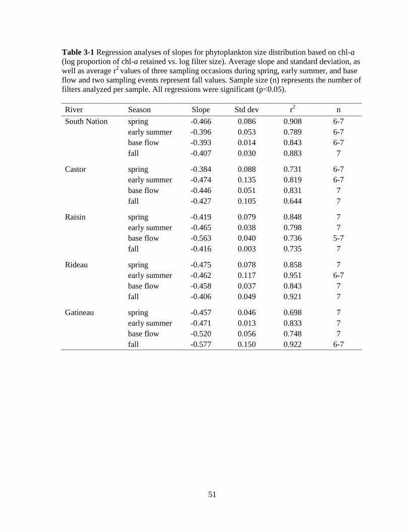
51
Table 3-1 Regression analyses of slopes for phytoplankton size distribution based on chl-a
(log proportion of chl-a retained vs. log filter size). Average slope and standard deviation, as
well as average r2
values of three sampling occasions during spring, early summer, and base
flow and two sampling events represent fall values. Sample size (n) represents the number of
filters analyzed per sample. All regressions were significant (p<0.05).
River Season Slope Std dev r2 n
South Nation spring -0.466 0.086 0.908 6-7
early summer -0.396 0.053 0.789 6-7
base flow -0.393 0.014 0.843 6-7
fall -0.407 0.030 0.883 7
Castor spring -0.384 0.088 0.731 6-7
early summer -0.474 0.135 0.819 6-7
base flow -0.446 0.051 0.831 7
fall -0.427 0.105 0.644 7
Raisin spring -0.419 0.079 0.848 7
early summer -0.465 0.038 0.798 7
base flow -0.563 0.040 0.736 5-7
fall -0.416 0.003 0.735 7
Rideau spring -0.475 0.078 0.858 7
early summer -0.462 0.117 0.951 6-7
base flow -0.458 0.037 0.843 7
fall -0.406 0.049 0.921 7
Gatineau spring -0.457 0.046 0.698 7
early summer -0.471 0.013 0.833 7
base flow -0.520 0.056 0.748 7
fall -0.577 0.150 0.922 6-7
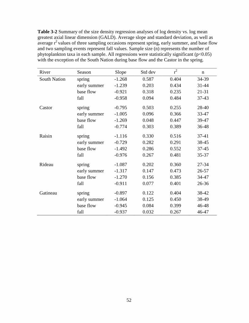
52
Table 3-2 Summary of the size density regression analyses of log density vs. log mean
greatest axial linear dimension (GALD). Average slope and standard deviation, as well as
average r2
values of three sampling occasions represent spring, early summer, and base flow
and two sampling events represent fall values. Sample size (n) represents the number of
phytoplankton taxa in each sample. All regressions were statistically significant (p<0.05)
with the exception of the South Nation during base flow and the Castor in the spring.
River Season Slope Std dev r2 n
South Nation spring -1.268 0.587 0.404 34-39
early summer -1.239 0.203 0.434 31-44
base flow -0.921 0.318 0.235 21-31
fall -0.958 0.094 0.484 37-43
Castor spring -0.795 0.503 0.255 28-40
early summer -1.005 0.096 0.366 33-47
base flow -1.269 0.048 0.447 39-47
fall -0.774 0.303 0.389 36-48
Raisin spring -1.116 0.330 0.516 37-41
early summer -0.729 0.282 0.291 38-45
base flow -1.492 0.286 0.552 37-45
fall -0.976 0.267 0.481 35-37
Rideau spring -1.087 0.202 0.360 27-34
early summer -1.317 0.147 0.473 26-57
base flow -1.270 0.156 0.385 34-47
fall -0.911 0.077 0.401 26-36
Gatineau spring -0.897 0.122 0.404 38-42
early summer -1.064 0.125 0.450 38-49
base flow -0.945 0.084 0.399 46-48
fall -0.937 0.032 0.267 46-47
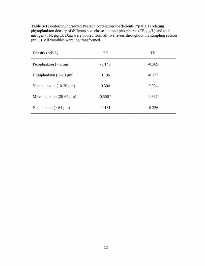
53
Table 3-3 Bonferroni corrected Pearson correlation coefficients (*p<0.01) relating
phytoplankton density of different size classes to total phosphorus (TP, μg/L) and total
nitrogen (TN, μg/L). Data were pooled from all five rivers throughout the sampling season
(n=55). All variables were log transformed.
Density (cell/L) TP TN
Picoplankton (< 2 µm) -0.143 -0.369
Ultraplankton ( 2-10 µm) 0.196 -0.177
Nanoplankton (10-20 µm) 0.304 0.004
Microplankton (20-64 µm) 0.506* 0.367
Netplankton (> 64 µm) -0.131 -0.236
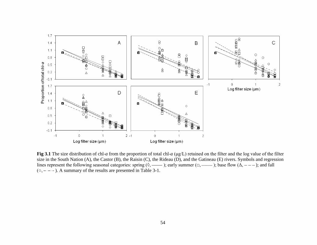
54
Fig 3.1 The size distribution of chl-a from the proportion of total chl-a (μg/L) retained on the filter and the log value of the filter
size in the South Nation (A), the Castor (B), the Raisin (C), the Rideau (D), and the Gatineau (E) rivers. Symbols and regression
lines represent the following seasonal categories: spring (◊, ); early summer (□, ); base flow (Δ, ); and fall
(○, ). A summary of the results are presented in Table 3-1.
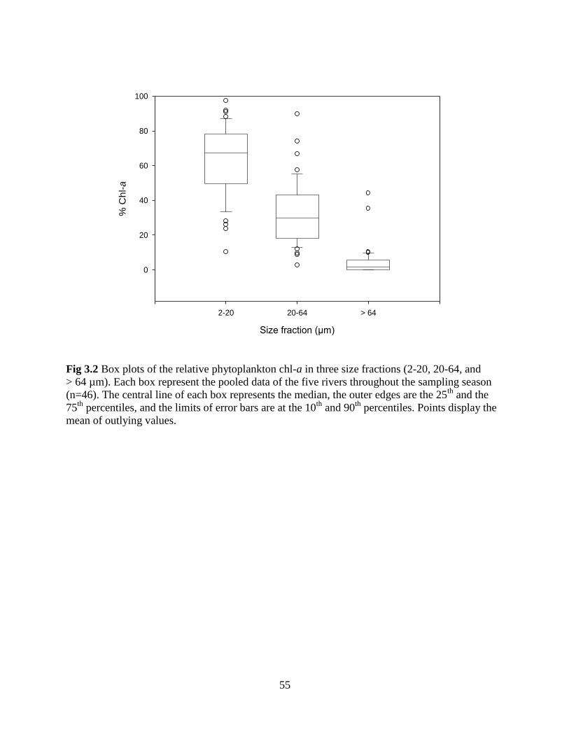
55
Fig 3.2 Box plots of the relative phytoplankton chl-a in three size fractions (2-20, 20-64, and
> 64 µm). Each box represent the pooled data of the five rivers throughout the sampling season
(n=46). The central line of each box represents the median, the outer edges are the 25th
and the
75th
percentiles, and the limits of error bars are at the 10th
and 90th
percentiles. Points display the
mean of outlying values.
Size fraction (µm)
2-20 20-64 > 64
% C
hl-a
0
20
40
60
80
100
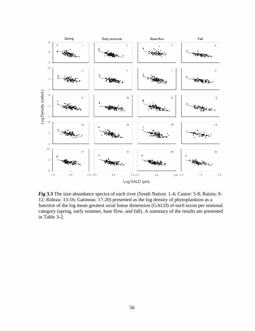
56
Fig 3.3 The size-abundance spectra of each river (South Nation: 1-4; Castor: 5-8; Raisin; 9-
12; Rideau: 13-16; Gatineau: 17-20) presented as the log density of phytoplankton as a
function of the log mean greatest axial linear dimension (GALD) of each taxon per seasonal
category (spring, early summer, base flow, and fall). A summary of the results are presented
in Table 3-2.
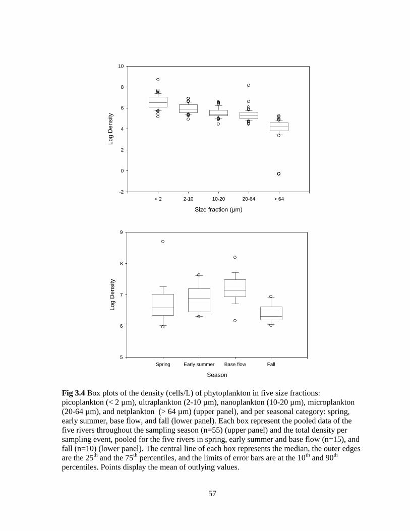
57
Size fraction (µm)
< 2 2-10 10-20 20-64 > 64
Lo
g D
en
sity
-2
0
2
4
6
8
10
Season
Spring Early summer Base flow Fall
Lo
g D
en
sity
5
6
7
8
9
Fig 3.4 Box plots of the density (cells/L) of phytoplankton in five size fractions:
picoplankton (< 2 µm), ultraplankton (2-10 µm), nanoplankton (10-20 µm), microplankton
(20-64 µm), and netplankton (> 64 µm) (upper panel), and per seasonal category: spring,
early summer, base flow, and fall (lower panel). Each box represent the pooled data of the
five rivers throughout the sampling season (n=55) (upper panel) and the total density per
sampling event, pooled for the five rivers in spring, early summer and base flow (n=15), and
fall (n=10) (lower panel). The central line of each box represents the median, the outer edges
are the 25th
and the 75th
percentiles, and the limits of error bars are at the 10th
and 90th
percentiles. Points display the mean of outlying values.
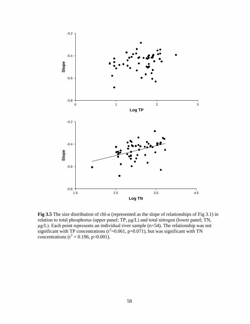
58
Fig 3.5 The size distribution of chl-a (represented as the slope of relationships of Fig 3.1) in
relation to total phosphorus (upper panel; TP, μg/L) and total nitrogen (lower panel; TN,
μg/L). Each point represents an individual river sample (n=54). The relationship was not
significant with TP concentrations (r2=0.061, p=0.071), but was significant with TN
concentrations (r2 = 0.196, p<0.001).
-0.8
-0.6
-0.4
-0.2
0 1 2 3
Slo
pe
Log TP
-0.8
-0.6
-0.4
-0.2
1.5 2.5 3.5 4.5
Slo
pe
Log TN
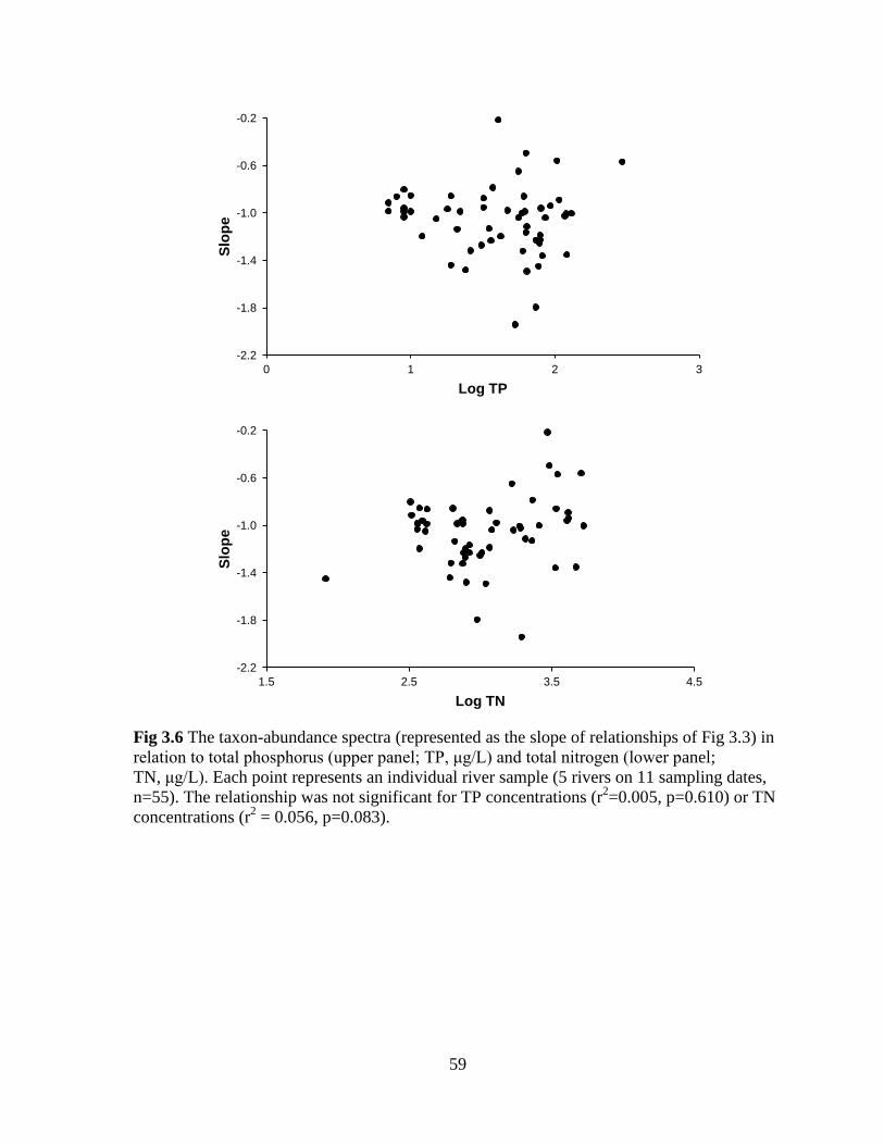
59
Fig 3.6 The taxon-abundance spectra (represented as the slope of relationships of Fig 3.3) in
relation to total phosphorus (upper panel; TP, μg/L) and total nitrogen (lower panel;
TN, μg/L). Each point represents an individual river sample (5 rivers on 11 sampling dates,
n=55). The relationship was not significant for TP concentrations (r2=0.005, p=0.610) or TN
concentrations (r2 = 0.056, p=0.083).
-2.2
-1.8
-1.4
-1.0
-0.6
-0.2
0 1 2 3
Slo
pe
Log TP
-2.2
-1.8
-1.4
-1.0
-0.6
-0.2
1.5 2.5 3.5 4.5
Slo
pe
Log TN
- Chapter 4 -
Seasonal succession of phytoplankton taxa
in temperate rivers and response to environmental factors
61
Abstract
The taxonomic composition of phytoplankton communities was assessed throughout a
growing season in five temperate rivers ranging in trophic state (9-107 µg/L total
phosphorus) to determine the impact of major environmental factors such as nutrients and
flow on community structure. Even though diatoms were on average the most important
division (38% of total biomass) in four of the five rivers, other taxonomic divisions were also
important. Cryptophytes (mainly Cryptomonas) rather than diatoms dominated biomass in
the mesoeutrophic Rideau River. More eutrophic rivers showed stronger overall dominance
of particular taxa. A bloom of colonial green alga (Pandorina morum) accounted for as much
as 90% of total biomass in the more nutrient enriched system compared to the highest
dominance (34%) found in the oligotrophic Gatineau River. Despite differences in
dominance patterns, the overall species richness was independent of trophic state and fairly
constant (the median number of taxa in individual samples ranged from 30 to 39). Seasonal
succession differed across the five rivers and no consistent pattern emerged such as described
for lakes. Collectively, a negative response to water discharge was found for diatoms,
cryptophytes, chlorophytes, and euglenoids while reactive and total phosphorus were
positively associated with euglenoids. Chrysophytes biomass decreased with increasing
nitrate concentrations and diatoms were positively correlated with total nitrogen.
62
4.1 Introduction
The study of phytoplankton taxonomic composition provides more valuable
information than aggregate measures of community structure such as algal biomass
(chlorophyll-a) and size distribution analyses (e.g. Sabater et al., 2008). Changes in
environmental conditions can shift phytoplankton species composition and alter ecosystem
processes, function, and stability which makes understanding taxonomic changes important
for ecosystem management (e.g. Suikkanen et al., 2007). In lakes, it has been well
established that phytoplankton community composition and diversity change with increasing
nutrients (Reynolds, 1984). These changes occur because of the different nutrient uptake,
storage, growth, and loss rates among different phytoplankton taxa (Kalff and Knoechel,
1978; Reynolds, 1984). However, in rivers, phytoplankton communities have not been as
intensively studied and are still poorly understood (Basu and Pick, 1996; Piirsoo et al., 2008;
Wu et al., 2011).
In temperate rivers, diatoms are considered to be the most important taxonomic group
both in terms of abundance and biomass (Rojo et al., 1994). Diatom based studies have
observed that shifts in species composition can provide evidence of anthropogenic impacts
(e.g. Lowe, 1974; Yang et al., 1996) and the presence of certain species can be indicative of
the state of the ecosystem. For example, Aulacoseira granulata and Stephanodiscus parvus
are diatom species representative of nutrient enriched lakes and typically bloom in highly
eutrophic European rivers, dominating total algal biomass (Moss and Balls, 1989; Rojo et al.,
1994; Cumming et al., 1995). However, other phytoplankton taxonomic groups can
constitute an important component of total abundance and biomass. In a survey of 67 rivers,
Rojo et al. (1994) found that diatoms represented 40% of the average number of species in
temperate rivers, yet green algae contributed 28%, cyanobacteria 10%, and euglenoids 7%. A
63
study of 31 temperate rivers in Ontario and Quebec observed that diatoms also dominated
phytoplankton biomass (34% of total); however, other divisions were also significant to total
biomass (Chételat et al., 2006). These divisions were cryptophytes (24%), chlorophytes and
chrysophytes (15%); in contrast, cyanobacteria were not well represented (3%). Therefore, it
is important to consider other lesser known phytoplankton groups besides diatoms.
In lakes, phytoplankton distribution patterns are strongly correlated with
environmental variables (Reynolds, 1984; Kalff, 2002). However, in rivers, it can be difficult
to determine if hydrological, physical, chemical, or biological factors are most important in
controlling community composition (Basu and Pick, 1995). Some studies have indicated that
nutrients such as phosphorus concentration control phytoplankton biomass (e.g. Søballe and
Kimmel, 1987; Basu and Pick, 1996; Van Nieuwenhuyse and Jones, 1996) while other
studies have indicated that hydrological conditions are more important to phytoplankton
development (e.g. Pace et al., 1992; Reynolds et al., 1994). In rivers as in lakes, dissolved
silicate is particularly important to sustain diatom growth as it is needed to build their cell
walls (Bormans and Webster, 1999). When concentrations of silica are depleted in rivers,
this can lead to a collapse in diatom populations (De Ruyter van Steveninck et al., 1992).
Although this does not affect algal biomass, it can explain shifts in phytoplankton
community abundance.
Classic lake phytoplankton seasonal succession models such as the Plankton Ecology
Group-model for temperate lakes (Sommer et al., 1986) may not be readily applied to rivers
as different factors may be controlling phytoplankton development (e.g. short water
residence times and/or weak top-down control from zooplankton). However, early river
studies have observed patterns such as diatom blooms in the spring, followed by shifts of
dominance between green algae and cyanobacteria in the summer months, and then
64
dominance of diatoms and/or dinoflagellates in the fall (Lewis, 1978). In the Rideau River,
phytoplankton seasonal succession was observed with high diatom biomass in early summer
followed by cryptophytes and chlorophyte dominance in the late summer (Yang et al., 1997;
Ley and Hamilton, 1995; Ley et al., 1997). However, very few studies have analyzed
seasonal patterns of phytoplankton species composition in rivers (Reynolds and Descy, 1996;
Gosselain and Descy, 2001) and more studies are needed to determine seasonal patterns
across rivers ranging in environmental conditions.
The objectives of this study were to: (i) describe the seasonal succession of
phytoplankton in five temperate rivers ranging in environmental conditions and (ii) to
determine the main drivers of community structure across the rivers. I hypothesized that
phytoplankton seasonal succession will vary per river because of different flow and nutrient
dynamics and that dominance patterns will be related to nutrient concentrations across the
rivers.
4.2 Methods
4.2.1 Study sites
Samples were collected from five temperate Ontario and Quebec rivers ranging in
land use and nutrient concentrations. River descriptions and hydrological regimes are
summarized in Chapter 2 (Table 2-1). For this study, discharge values were obtained by
calculating the average daily discharges seven days prior to and including water collection
dates (Pace et al., 1992; Basu and Pick, 1996).
65
4.2.2 River sampling and laboratory analyses
Each river was sampled every two weeks from late May until early November 2009.
On occasion, sampling was postponed for a minimum of two days following major rain
events. A total of 11 samples were collected per river to represent phytoplankton
communities and river conditions over the growing season (Chételat and Pick, 2001). Water
was collected in Nalgene bottles mid-channel where rivers are typically deepest. The bottles
were triple rinsed with river water before collecting subsurface grab samples. In situ water
measurements of temperature, dissolved oxygen (DO), dissolved oxygen percent saturation
(%DO), pH, and conductivity (SPC) were taken with a Hydrolab Minisonde Multiprobe 4a.
Turbidity was determined in the laboratory using a LaMotte 2020 turbidimeter following
every sampling event. Turbidity readings represent the ratio between the scattered light at 90
and 180 degrees from the light source and are given in Nephelometric Turbidity Units
(NTU).
The water collected from each site was preserved in Lugol’s iodine solution for
phytoplankton identification. Water samples were also brought to the City of Ottawa’s
Robert O. Pickard Environmental Centre for nutrient analysis using standard methods (Basu
and Pick, 1995). The nutrients analyzed were: total phosphorus (TP), reactive phosphorus
(RP), total Kjeldahl nitrogen (TKN), nitrate+nitrite (N03+N02), and ammonia+ammonium
(NH3+NH4+). Total nitrogen (TN) was calculated by adding TKN to N03+N02. In late May
and late August samples were also analyzed for silica concentrations.
As a measure of total algal biomass, chlorophyll-a (chl-a) concentrations were
determined by filtering 250 mL of water through 0.2 μm polycarbonate membranes. When
filtering the water, vacuum pressure was set below 15 mm Hg to avoid cell breakage.
Following filtration, filters were stored at -25°C until they were processed. Chl-a was
66
extracted by adding 15 mL of ethanol to each sample for a minimum of 24 hours, and
concentrations were estimated with a Cary® 100 BIO UV-Visible Spectrophotometer,
Varian Inc (Jespersen and Christoffersen, 1987).
4.2.3 Phytoplankton identification and enumeration
Phytoplankton identification and enumerations were made using a Zeiss AXIO A1
inverted microscope equipped with an Empix camera and an Eclipse image analysis system.
Phytoplankton preserved in Lugol’s that were greater than 2 μm were identified, counted and
measured under light microscopy at X200, X400, and X630 magnifications. Ten mL of
Lugol’s preserved water samples were settled overnight in 26 mm diameter chambers and the
enumeration of a minimum of 300 cells per sample were made following the Utermöhl
method (Lund et al., 1958). Counts and cell dimensions were recorded using the computer
counting program, Algamica, version 4.0 (Gosselain and Hamilton, 2000). Algamica
calculates cell density (cells/L) and biomass (mg/m3) based on dimensions measured for each
taxon per sample. Phytoplankton were identified as much as possible to the highest
resolution (~ genus/species). When species identification was not possible, cells were
counted in the correct division as unknown species. Therefore, different taxa were accounted
for but the species name could not always be confirmed. For example, the Chryptomonas
genus of the cryptophyte division was separated into species one through four based on size
and shape (Appendix 4). Similarly, centric diatoms were identified as Stephanodiscus or
Cyclotella based on size (Appendix 5). Species identification of these genera would have
required separate observations with a Scanning Electron Microscope (SEM) as many of them
were quite small. Algamica also computes total phytoplankton density, biomass, and number
of taxa for 12 algal divisions. However, half were dismissed due to low abundance and
67
biomass and only the following divisions were considered in the analyses: Bacillariophyta
(diatoms), Cryptophyta (cryptophytes), Chlorophyta (geen-algae), Euglenophyta
(euglenoids), Chrysophyta (chrysophytes), and Pyrrhophyta (dinoflagellates).
4.2.4 Data analysis
Seasonal data were pooled into four time periods: spring, early summer, base flow,
and fall. Spring was based on three sampling occurrences from late May until end of June,
representing the period of declining discharge. The early summer category consisted of three
sampling dates covering July to early August. Since during 2009 heavy rain was recorded
throughout the month of July, base flow conditions occurred later during the ice-free season;
late August and September (n=3) represented base flow conditions. Fall samples were
represented by two sampling dates that took place in October and early November when the
flows tend to rise again.
Taxa dominance occurs when a significant amount of the total biomass (> 30%) in a
sample is represented by one taxa. However, when only one or two cells were identified in a
sample and accounted for a high percentage of biomass (~ 10%), these rare (yet very large)
taxa were removed from the analysis. To further reduce the impact of extreme values,
biomass estimates were log transformed.
Bonferroni adjusted Pearson correlations coefficients were calculated to determine
the response of phytoplankton biomass to physical, chemical, and biological variables in the
six taxonomic divisions. Variables were log transformed to satisfy normality and all
statistical analyses were done with S-Plus® version 8.0.
68
4.3 Results
4.3.1 Physical and chemical variables
Physical and chemical parameters varied throughout the study period and across the
different rivers. A summary of these variables can be found in Chapter 2 (Fig 2.1,
Appendix 1).
4.3.2 Phytoplankton seasonal succession
South Nation River
In the South Nation River, diatoms had the highest median biomass of all the
divisions encountered (Table 4-2). However, seasonally, dominance shifted between
diatoms, chlorophytes, and cryptophytes (Fig 4.2). On August 25, chlorophytes dominated at
96% of total biomass (36,522 mg/m3) caused by a bloom of the colonial motile species
Pandorina morum (Fig 4.2; Appendix 6). In the weeks prior to and following the bloom, its
abundance increased from 6.8x10³ cells/L on August 11 to 135x10
6 cells/L at the peak and
declined to 143x103 cells/L on September 10. This was the only occurrence of green alga
dominance found in this study. Throughout the ice-free period, cryptophytes (mainly
Cryptomonas) consistently represented more than 15% of total biomass (Table 4-1). A
colonial centric diatom, Melosira was also significant contributing 19 to 28% of the
phytoplankton biomass in spring, early summer, and fall (Table 4-1).
Castor River
On average, diatoms dominated phytoplankton biomass in the Castor River
(Table 4-2) and also on most dates during the ice-free season (Fig 4.2). Very high diatom
dominance was observed in the spring and fall (93%). The centric diatom Stephanodiscus
69
was present in all seasonal categories and represented as much as 55% of total biomass
during base flow (Table 4-1; Appendix 7). One decline in diatoms occurred during spring
and the other occurred during base flow when cryptophytes (mostly Cryptomonas)
represented 42% of the total biomass. The Castor was the only river with very high
euglenoid biomass: during base flow and fall, Euglena represented 23% and 13% of total
phytoplankton biomass (Table 4-1).
Raisin River
Diatoms had yet again the highest biomass on average compared to the other
taxonomic groups (Table 4-2). Seasonally, the Raisin River was a very dynamic system with
six major taxonomic divisions fluctuating in their relative importance (Fig. 4.1).
Cryptophytes (Cryptomonas) was the most important division and represented often more
than 40% of total phytoplankton biomass, dominating in all seasonal categories except early
summer when the diatom Melosira dominated (78%) (Fig 4.2; Table 4-1; Appendix 8).
Rideau River
In contrast to the other four rivers, the Rideau River was on average dominated by
cryptophytes (Fig 4.2; Table 4-2). In the spring, Cryptomonas showed high dominance
(83%) and continuously dominated total biomass across the seasons (Table 4-1). Diatoms
had high percent biomass on three sampling events (early summer and base flow) with
Fragilaria and Aulacoseira as the taxa representing the most biomass (Fig 4.2 and
Appendix 9). Chrysophytes had high individual contribution to total biomass during spring
(Dinobrynon divergens) and fall (Synura uvella) (Table 4-1). The Rideau River was the only
70
system where pyrrhophyta (mainly Peridinium) represented more than 15% biomass (three
sampling dates, Table 4-1).
Gatineau River
Overall, biomass was much lower in the Gatineau River than in the other rivers
(Table 4-2). Diatoms had the highest median biomass, then cryptophytes followed closely by
chrysophytes and chlorophytes. The Gatineau River had lower dominance of individual taxa
compared to the other rivers (Fig 4.2). The highest taxa dominance observed was a colonial
chrysophyte (Dinobryon divergens), that reached 34% of total phytoplankton biomass
(Table 4-1) in spring. All other taxa represented individually less than 30% of total biomass.
This was different from the other rivers of this study where at least once, a specific taxon
accounted for greater than 50% of total biomass. The main diatom taxa in the Gatineau were
Tabellaria, Melosira and Cocconeis while the cryptophytes were mainly represented by
Cryptomonas (Appendix 10).
Taxa diversity
The main algal divisions varied in species diversity across the different rivers
(Table 4-2). The number of taxa was highest for diatoms (7-11) and green algae (9-13).
Cryptophyte diversity ranged from 4 to 6 taxa while chrysophytes included 4 and 11.
Chrysophyte taxa diversity was highest in the most oligotrophic system: the Gatineau River
had 8 to 12 taxa. Across all rivers, the median value of total taxa in a given sample varied
from 30 to 39, regardless of system trophy. Both a eutrophic (Castor) and an oligotrophic
river (Gatineau) had the highest median number of taxa (39). The maximum species diversity
was observed in the Rideau River (51) and the second highest (46) was found in the Castor
71
River. The lowest number of taxa (20) was observed in the South Nation River during the
Pandorina morum bloom.
4.3.3 Phytoplankton taxonomic divisions and response to environmental variables
The biomass of the main algal divisions responded differently to physical, chemical,
and biological factors (Table 4-3). When all the rivers and samples were considered, positive
and significant correlations were observed between pH and diatoms, cryptophytes, and green
algae. Green algae were the only phytoplankton division to show a positive association with
temperature while diatoms and euglenoids responded positively to conductivity. Water
discharge lead to negative correlations for the majority of the phytoplankton divisions:
diatoms, cryptophytes, chlorophytes, and euglenoids. In contrast, the response of the
divisions to nutrients varied from positive to negative and was often not statistically
significant. However, euglenoids responded positively and significantly to phosphorus (both
as RP and TP). Chrysophytes had a negative association with nitrate, and diatoms tended to
increase with total nitrogen concentrations. Total algal chl-a was positively correlated with
diatoms, chlorophytes, chrysophyes, and euglenoids.
4.4 Discussion
No common pattern in the phytoplankton communities was observed across the
different rivers (e.g. Fig 4.1). There was a lack of a common periodicity in seasonal
succession as has been described for decades in lakes and now modeled (Sommer et al.,
1986). For example, while diatoms were often most prominent in the spring and fall as in
lakes, this was not the case for all rivers. Diatoms were also important during summer and
during base flow.
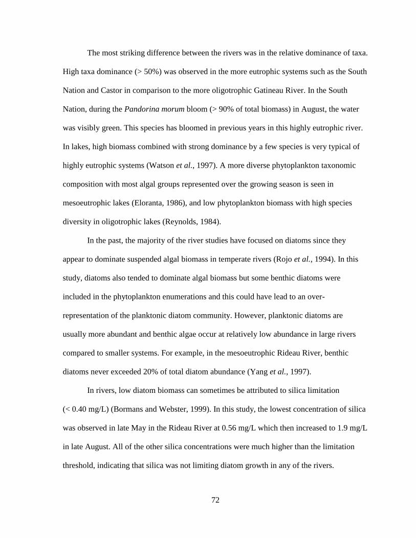
72
The most striking difference between the rivers was in the relative dominance of taxa.
High taxa dominance (> 50%) was observed in the more eutrophic systems such as the South
Nation and Castor in comparison to the more oligotrophic Gatineau River. In the South
Nation, during the Pandorina morum bloom (> 90% of total biomass) in August, the water
was visibly green. This species has bloomed in previous years in this highly eutrophic river.
In lakes, high biomass combined with strong dominance by a few species is very typical of
highly eutrophic systems (Watson et al., 1997). A more diverse phytoplankton taxonomic
composition with most algal groups represented over the growing season is seen in
mesoeutrophic lakes (Eloranta, 1986), and low phytoplankton biomass with high species
diversity in oligotrophic lakes (Reynolds, 1984).
In the past, the majority of the river studies have focused on diatoms since they
appear to dominate suspended algal biomass in temperate rivers (Rojo et al., 1994). In this
study, diatoms also tended to dominate algal biomass but some benthic diatoms were
included in the phytoplankton enumerations and this could have lead to an over-
representation of the planktonic diatom community. However, planktonic diatoms are
usually more abundant and benthic algae occur at relatively low abundance in large rivers
compared to smaller systems. For example, in the mesoeutrophic Rideau River, benthic
diatoms never exceeded 20% of total diatom abundance (Yang et al., 1997).
In rivers, low diatom biomass can sometimes be attributed to silica limitation
(< 0.40 mg/L) (Bormans and Webster, 1999). In this study, the lowest concentration of silica
was observed in late May in the Rideau River at 0.56 mg/L which then increased to 1.9 mg/L
in late August. All of the other silica concentrations were much higher than the limitation
threshold, indicating that silica was not limiting diatom growth in any of the rivers.
73
In rivers, there also tends to be high biomass of centric compared to pennate diatoms
as they have higher growth rates and lower sinking losses (Corbelas and Rojo, 1994). In the
Warnow River, high centric diatom biomass has been observed in the spring and in autumn
(Bahnwart et al., 1998). Similarly, this study observed high biomass of the centric diatoms,
Stephanodiscus and Cyclotella. In particular, high Stephanodicus biomass was noted
throughout the growing season with the highest dominance occurring from summer to early
fall in the Castor River. Scanning Electron Microscope (SEM) studies would confirm
whether the species were the same as typically found in eutrophic European rivers (e.g. S.
hantzschii) (Hasle and Fryxell, 1970).
The only river that did not show diatom biomass dominance was the Rideau River
where cryptophytes accounted for almost half of the total biomass. Cryptophytes are known
to proliferate in slow flowing water and are able to control their sinking rates through flagella
motion which give them an advantage over other species under light limiting conditions
(Bahnwart et al., 1998). The Rideau River is a more regulated river than the others (as part of
the Rideau Canal system operated by Parks Canada) and water residence times at the Baxter
sampling site may have represented more lake-like conditions than the other river sites.
However, the Rideau River had the lowest light extinction coefficients and lowest turbidity
(Appendix 1) compared to the other rivers and was thus the least likely to be light limited.
The strong negative response of diatoms, cryptophytes, chlorophytes, and euglenoids
to water discharge observed in this study is in agreement with past studies indicating the
strong impact that hydrological regimes have on phytoplankton development in rivers
(Descy, 1987; Piirsoo et al., 2008). In this study, cyanobacteria were observed occasionally;
however, they were not important contributors to total biomass, as found in previous studies,
likely because they are less competitive under the high water turbulence of rivers
74
(Moss et al., 1984; Chételat et al., 2006). During this study period of 2009, the river
discharge was generally higher than the historical average due to high precipitation,
especially during July. Significant rain events (> 30 mm) can increase discharge and
decrease algal biomass as much as 100 fold over short periods of time in the Rideau,
however, phytoplankton communities can recover in less than seven days (Ley et al., 1997).
While some studies have reported positive response of all taxonomic phytoplankton
group biomass to TP in lakes (Watson et al., 1997), the results of this study only found a
significant positive correlation between euglenoids and phosphorus concentrations. Results
also indicated a negative response of the chrysophyte group to nitrate concentrations and a
positive association between diatoms and nitrogen concentrations was observed. The diatom
response to TN corresponds to results of previous studies that have observed changes in
diatom biomass with total nitrogen concentrations (Yang et al., 1997).
Taxonomic resolution to species level would provide additional information on the
state of rivers and allow for more complex multivariate statistical analyses. However, more
sophisticated laboratory analyses such as SEM are needed to confirm identification,
especially for diatoms. It is important to keep in mind that this study provided correlations
between phytoplankton communities and environmental variables that may have some
predictive value; however these correlations may not reflect direct causal associations.
Establishing causal relationships in rivers is difficult since in situ manipulations and
experimentation are usually not feasible at the relevant scales.
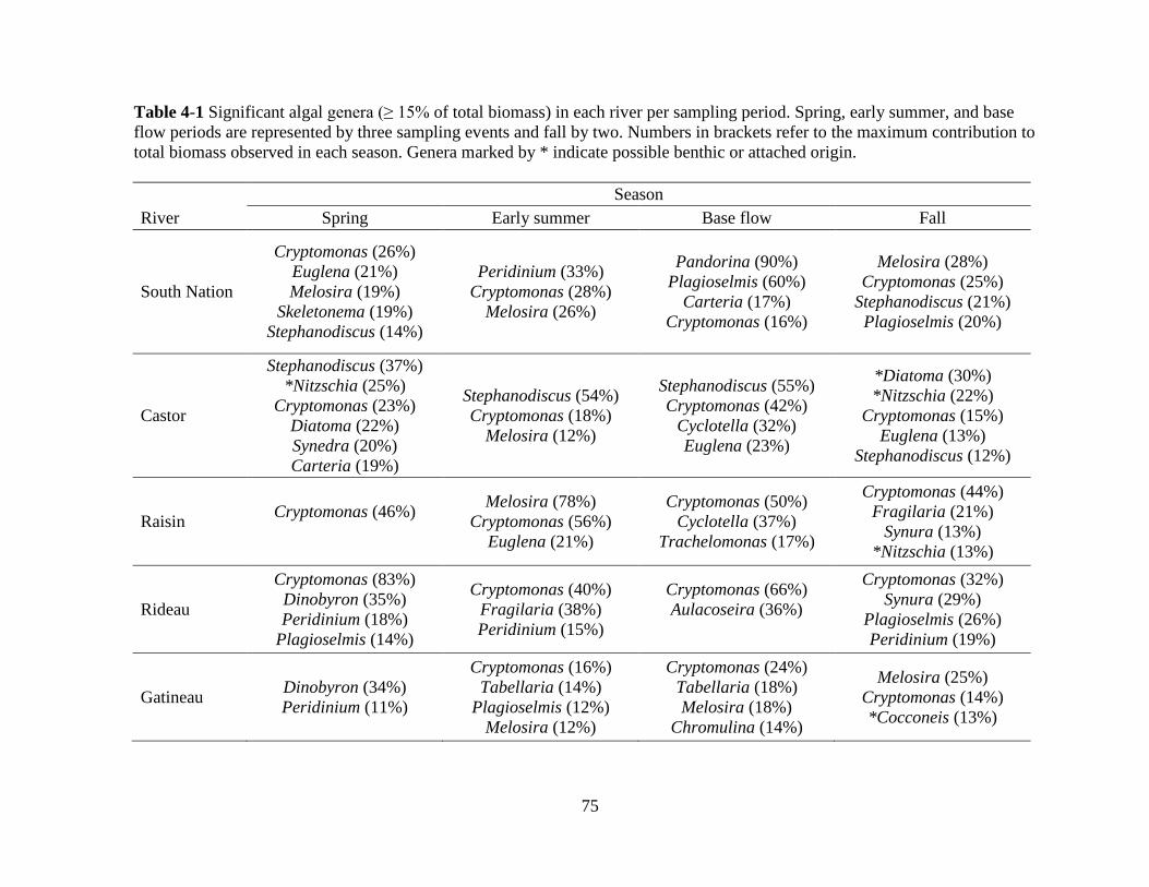
75
Table 4-1 Significant algal genera (≥ 15% of total biomass) in each river per sampling period. Spring, early summer, and base
flow periods are represented by three sampling events and fall by two. Numbers in brackets refer to the maximum contribution to
total biomass observed in each season. Genera marked by * indicate possible benthic or attached origin.
Season
River Spring Early summer Base flow Fall
South Nation
Cryptomonas (26%)
Euglena (21%)
Melosira (19%)
Skeletonema (19%)
Stephanodiscus (14%)
Peridinium (33%)
Cryptomonas (28%)
Melosira (26%)
Pandorina (90%)
Plagioselmis (60%)
Carteria (17%)
Cryptomonas (16%)
Melosira (28%)
Cryptomonas (25%)
Stephanodiscus (21%)
Plagioselmis (20%)
Castor
Stephanodiscus (37%)
*Nitzschia (25%)
Cryptomonas (23%)
Diatoma (22%)
Synedra (20%)
Carteria (19%)
Stephanodiscus (54%)
Cryptomonas (18%)
Melosira (12%)
Stephanodiscus (55%)
Cryptomonas (42%)
Cyclotella (32%)
Euglena (23%)
*Diatoma (30%)
*Nitzschia (22%)
Cryptomonas (15%)
Euglena (13%)
Stephanodiscus (12%)
Raisin Cryptomonas (46%)
Melosira (78%)
Cryptomonas (56%)
Euglena (21%)
Cryptomonas (50%)
Cyclotella (37%)
Trachelomonas (17%)
Cryptomonas (44%)
Fragilaria (21%)
Synura (13%)
*Nitzschia (13%)
Rideau
Cryptomonas (83%)
Dinobyron (35%)
Peridinium (18%)
Plagioselmis (14%)
Cryptomonas (40%)
Fragilaria (38%)
Peridinium (15%)
Cryptomonas (66%)
Aulacoseira (36%)
Cryptomonas (32%)
Synura (29%)
Plagioselmis (26%)
Peridinium (19%)
Gatineau Dinobyron (34%)
Peridinium (11%)
Cryptomonas (16%)
Tabellaria (14%)
Plagioselmis (12%)
Melosira (12%)
Cryptomonas (24%)
Tabellaria (18%)
Melosira (18%)
Chromulina (14%)
Melosira (25%)
Cryptomonas (14%)
*Cocconeis (13%)
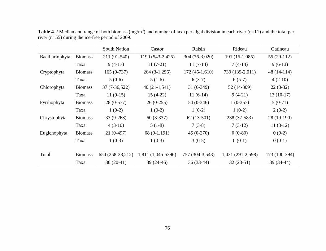
76
Table 4-2 Median and range of both biomass (mg/m3) and number of taxa per algal division in each river (n=11) and the total per
river (n=55) during the ice-free period of 2009.
South Nation Castor Raisin Rideau Gatineau
Bacillariophyta Biomass 211 (91-540) 1190 (543-2,425) 304 (76-3,020) 191 (15-1,085) 55 (29-112)
Taxa 9 (4-17) 11 (7-21) 11 (7-14) 7 (4-14) 9 (6-13)
Cryptophyta Biomass 165 (0-737) 264 (3-1,296) 172 (45-1,610) 739 (139-2,011) 48 (14-114)
Taxa 5 (0-6) 5 (1-6) 6 (3-7) 6 (5-7) 4 (2-10)
Chlorophyta Biomass 37 (7-36,522) 40 (21-1,541) 31 (6-349) 52 (14-309) 22 (8-32)
Taxa 11 (9-15) 15 (4-22) 11 (6-14) 9 (4-21) 13 (10-17)
Pyrrhophyta Biomass 28 (0-577) 26 (0-255) 54 (0-346) 1 (0-357) 5 (0-71)
Taxa 1 (0-2) 1 (0-2) 1 (0-2) 1 (0-2) 2 (0-2)
Chrystophyta Biomass 33 (9-268) 60 (3-337) 62 (13-501) 238 (37-583) 28 (19-190)
Taxa 4 (3-10) 5 (1-8) 7 (3-8) 7 (3-12) 11 (8-12)
Euglenophyta Biomass 21 (0-497) 68 (0-1,191) 45 (0-270) 0 (0-80) 0 (0-2)
Taxa 1 (0-3) 1 (0-3) 3 (0-5) 0 (0-1) 0 (0-1)
Total Biomass 654 (258-38,212) 1,811 (1,045-5396) 757 (304-3,543) 1,431 (291-2,598) 173 (100-394)
Taxa 30 (20-41) 39 (24-46) 36 (33-44) 32 (23-51) 39 (34-44)
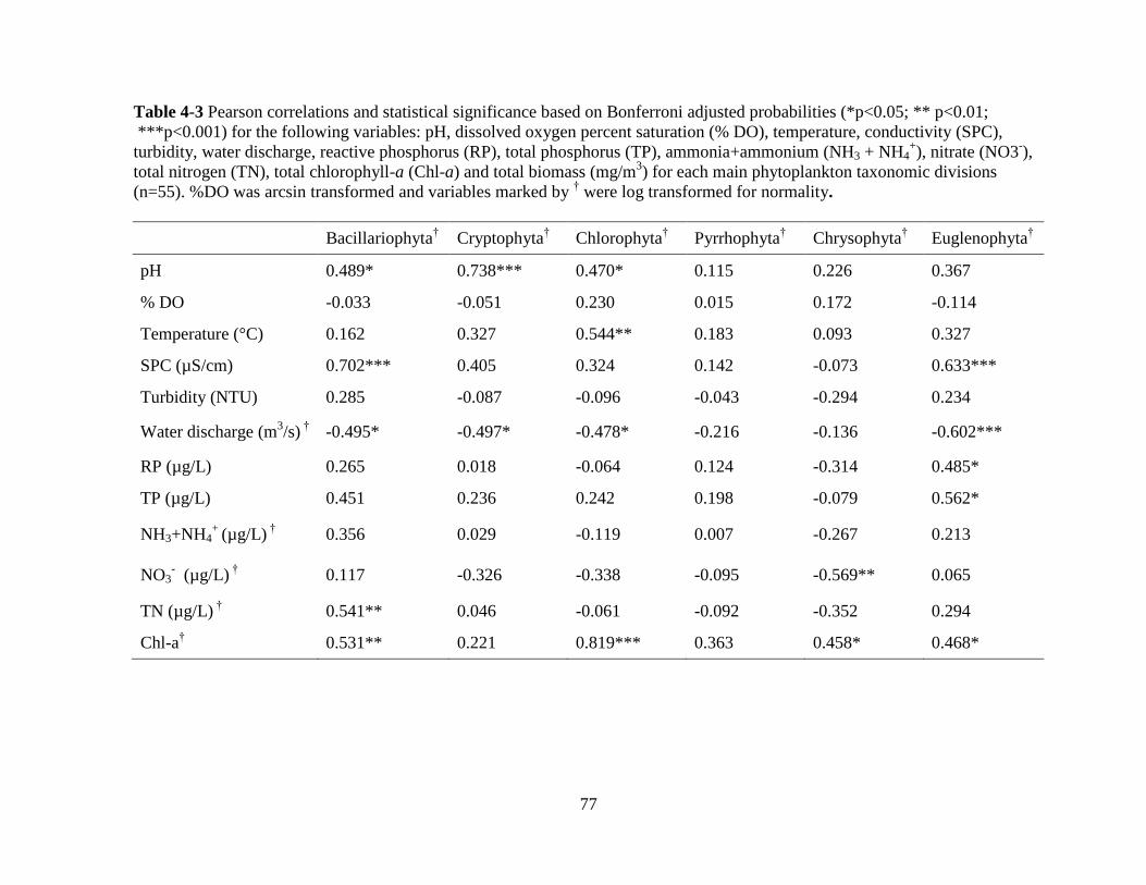
77
Table 4-3 Pearson correlations and statistical significance based on Bonferroni adjusted probabilities (*p<0.05; ** p<0.01;
***p<0.001) for the following variables: pH, dissolved oxygen percent saturation (% DO), temperature, conductivity (SPC),
turbidity, water discharge, reactive phosphorus (RP), total phosphorus (TP), ammonia+ammonium (NH3 + NH4+), nitrate (NO3
-),
total nitrogen (TN), total chlorophyll-a (Chl-a) and total biomass (mg/m3) for each main phytoplankton taxonomic divisions
(n=55). %DO was arcsin transformed and variables marked by † were log transformed for normality.
Bacillariophyta† Cryptophyta
† Chlorophyta
† Pyrrhophyta
† Chrysophyta
† Euglenophyta
†
pH 0.489* 0.738*** 0.470* 0.115 0.226 0.367
% DO -0.033 -0.051 0.230 0.015 0.172 -0.114
Temperature (°C) 0.162 0.327 0.544** 0.183 0.093 0.327
SPC (µS/cm) 0.702*** 0.405 0.324 0.142 -0.073 0.633***
Turbidity (NTU) 0.285 -0.087 -0.096 -0.043 -0.294 0.234
Water discharge (m3/s)
† -0.495* -0.497* -0.478* -0.216 -0.136 -0.602***
RP (µg/L) 0.265 0.018 -0.064 0.124 -0.314 0.485*
TP (µg/L) 0.451 0.236 0.242 0.198 -0.079 0.562*
NH3+NH4+
(µg/L) †
0.356 0.029 -0.119 0.007 -0.267 0.213
NO3- (µg/L)
† 0.117 -0.326 -0.338 -0.095 -0.569** 0.065
TN (µg/L) †
0.541** 0.046 -0.061 -0.092 -0.352 0.294
Chl-a† 0.531** 0.221 0.819*** 0.363 0.458* 0.468*
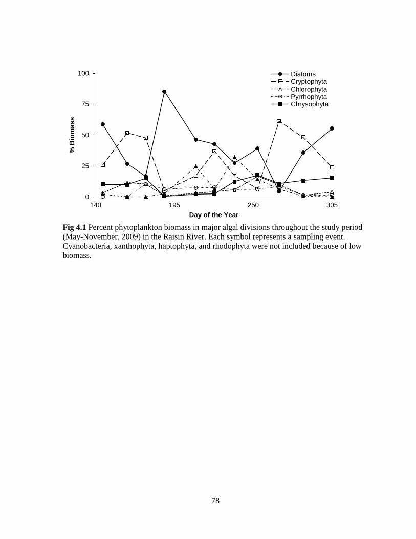
78
Fig 4.1 Percent phytoplankton biomass in major algal divisions throughout the study period
(May-November, 2009) in the Raisin River. Each symbol represents a sampling event.
Cyanobacteria, xanthophyta, haptophyta, and rhodophyta were not included because of low
biomass.
0
25
50
75
100
140 195 250 305
% B
iom
ass
Day of the Year
Diatoms Cryptophyta Chlorophyta Pyrrhophyta Chrysophyta
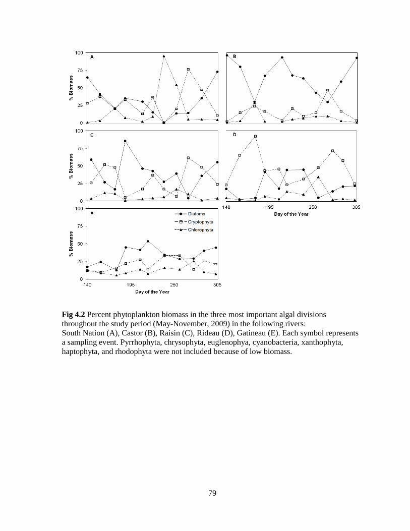
79
Fig 4.2 Percent phytoplankton biomass in the three most important algal divisions
throughout the study period (May-November, 2009) in the following rivers:
South Nation (A), Castor (B), Raisin (C), Rideau (D), Gatineau (E). Each symbol represents
a sampling event. Pyrrhophyta, chrysophyta, euglenophya, cyanobacteria, xanthophyta,
haptophyta, and rhodophyta were not included because of low biomass.

- Chapter 5 -
General Conclusion
81
The aim of this thesis was to examine the structure of phytoplankton communities in
rivers with a particular focus on the relative importance of small cells (< 20 μm) to biomass
and seasonal dynamics. While the smallest size fraction of the plankton typically dominates
oligotrophic lakes and oceans, picophytoplankton also contributed significantly to
chlorophyll-a (chl-a) and biomass in rivers, even in the most eutrophic systems. The analysis
of the size distribution of planktonic chl-a and taxa based abundance size spectra both
showed that phytoplankton communities were uniformly dominated by small cells
throughout the ice-free period. This dominance is perhaps a general response to constant
turbulence and lower average light climate compared to lakes. These typical river conditions
might also represent a favourable environment for phycocyanin-rich picocyanobacteria,
which could explain their dominance of the picophytoplankton assemblage. Higher nutrient
concentrations did not lead to the usual shift to large cells observed in lakes and oceans.
However, high nitrate concentrations coupled with high temperature represented optimal
conditions for picophytoplankton. The presence of small cells implies a high metabolic
turnover and as a result the productivity and nutrient cycling in rivers is also likely very high,
which might explain the higher fish yields observed in rivers compared to lakes
(Randall et al., 1994).
In contrast to the analysis of structure based on size, the taxonomic composition of
the five rivers was much more variable. Across the rivers, no consistent seasonal succession
pattern was observed. Diatoms dominated in all rivers with the exception of the Rideau River
where cryptophytes were the most important phytoplankton group. High taxa dominance
(> 50% of biomass) was common in the more eutrophic rivers but the number of taxa
observed was similar across all rivers, regardless of trophy. While some taxonomic divisions
responded positively to nutrients, water discharge negatively affected most phytoplankton
82
taxonomic divisions. However, the picophytoplankton community was not affected by
discharge.
Many new questions arise from this thesis requiring further investigation.
Phytoplankton identification to the species level would have allowed for more sophisticated
data analyses but involve more detailed work, in particular the use of a Scanning Electron
Microscope (SEM) for diatoms, which was beyond the scope of this study. With a higher
level of taxonomic resolution, the results could be analyzed with multivariate statistics to
identify indicator species. Principle component analyses (PCA) and cluster analyses could
also be used to find associations between phytoplankton taxa and environmental variables.
Since taxa of benthic origin can be brought to the surface in periods of high flow and
turbulence and can increase the biomass of phytoplankton divisions (e.g. large pennate
diatoms), identifying and removing these species from analyses could reduce biomass
variability. Furthermore, based on the results of this study, more rivers will need to be
examined to establish seasonal patterns. The Plankton Ecology Group-model was developed
based on many seasonal studies of numerous lakes (e.g. Sommer et al., 1986). Lastly, 2009
was an unusually high flow year and this might help explain the importance of discharge for
the phytoplankton communities. The patterns observed in this study might have been
different under a much lower discharge scenario. Rivers should be studied over many years
to capture different hydrological regimes (high and low flow years) in order to determine the
relative importance of flow vs. nutrients on phytoplankton communities.
83
References
Agawin, N. S. R., Duarte, C. M., & Agusti, S. (2000). Nutrient and temperature control of
the contribution of picoplankton to phytoplankton biomass and production. Limnology
and Oceanography, 45(3), 591-600.
Allan, J. D., & Castillo, M. M. (2007). Stream ecology: Structure and function of running
waters. Springer. The Netherlands, pp. 436.
Armstrong, R. A. (2003). A hybrid spectral representation of phytoplankton growth and
zooplankton response: The “control rod” model of plankton interaction. Deep Sea
Research Part II: Topical Studies in Oceanography, 50(22-26), 2895-2916.
Bahnwart, M., Hübener, T., & Schubert, H. (1998). Downstream changes in phytoplankton
composition and biomass in a lowland river–lake system (Warnow River, Germany).
Hydrobiologia, 391(1), 99-111.
Basu, B. K., & Pick, F. R. (1995). Longitudinal and seasonal development of planktonic
chlorophyll a in the Rideau River, Ontario. Canadian Journal of Fisheries and Aquatic
Sciences, 52(4), 804-815.
Basu, B. K., & Pick, F. R. (1996). Factors regulating phytoplankton and zooplankton
biomass in temperate rivers. Limnology and Oceanography, 41(7), 1572-1577.
Basu, B., & Pick, F. R. (1997). Phytoplankton and zooplankton development in a lowland,
temperate river. Journal of Plankton Research, 19(2), 237-253.
Bell, T., & Kalff, J. (2001). The contribution of picophytoplankton in marine and freshwater
systems of different trophic status and depth. Limnology and Oceanography, 46(5), 1243-
1248.
Biggs, B. J. F. (1988). Algal proliferations in New Zealand's shallow stony foothills-fed
rivers: Toward a predictive model. Internationale Vereinigung fuer Theoretische und
Angewandte Limnologie. Verhandlungen IVTLAP, 23(3), 1405-1411.
Bormans, M., & Webster, I. T. (1999). Modelling the spatial and temporal variability of
diatoms in the River Murray. Journal of Plankton Research, 21(3), 581-598.
Brown, J. H., Gillooly, J. F., Allen, A. P., Savage, V. M., & West, G. B. (2004). Toward a
metabolic theory of ecology. Ecology, 85(7), 1771-1789.
Burnison, B. (1980). Modified dimethyl sulfoxide (DMSO) extraction for chlorophyll
analysis of phytoplankton. Canadian Journal of Fisheries and Aquatic Sciences, 37(4),
729-733.
84
Callieri, C. (2008). Picophytoplankton in freshwater ecosystems: The importance of small-
sized phototrophs. Freshwater Reviews, 1(1), 1-28.
Callieri, C., & Piscia, R. (2002). Photosynthetic efficiency and seasonality of autotrophic
picoplankton in Lago Maggiore after its recovery. Freshwater Biology, 47(5), 941-956.
Callieri, C., & Stockner, J. G. (2002). Freshwater autotrophic picoplankton: A review.
Journal of Limnology, 61(1), 1-14.
Callieri, C., Modenutti, B., Queimalinos, C., Bertoni, R., & Balseiro, E. (2007). Production
and biomass of picophytoplankton and larger autotrophs in Andean ultraoligotrophic
lakes: differences in light harvesting efficiency in deep layers. Aquatic Ecology, 41(4),
511-523.
Caraco, N. F., Cole, J. J., Raymond, P. A., Strayer, D. L., Pace, M. L., Findlay, S. E. G., &
Fischer, D. T. (1997). Zebra mussel invasion in a large, turbid river: phytoplankton
response to increased grazing. Ecology, 78(2), 588-602.
Caron, D. A., Pick, F. R., & Lean, D. R. S. (1985). Chroococcoid cyanobacteria in Lake
Ontario: vertical and seasonal distributions during 1982. Journal of Phycology, 21(1),
171-175.
Cattaneo, A. (1987). Periphyton in lakes of different trophy. Canadian Journal of Fisheries
and Aquatic Sciences, 44(2), 296-303.
Cattaneo, A., Kerimian, T., Roberge, M., & Marty, J. (1997). Periphyton distribution and
abundance on substrata of different size along a gradient of stream trophy de Montréal.
Hydrobiologia, 354(1), 101-110.
Chételat, J., & Pick, F. R. (2001). Temporal variability of water chemistry in flowing waters
of the northeastern United States: does river size matter? Journal of the North American
Benthological Society, 20(3), 331-346.
Chételat, J., Pick, F. R., & Hamilton, P. B. (2006). Potamoplankton size structure and
taxonomic composition: Influence of river size and nutrient concentrations. Limnology
and Oceanography, 51(1), 681-689.
Cole, J. J., Caraco, N. F., & Peierls, B. L. (1992). Can phytoplankton maintain a positive
carbon balance in a turbid, freshwater, tidal estuary? Limnology and Oceanography,
37(8), 1608-1617.
Corbelas, M., & Rojo, C. (1994). Factors influencing the share of planktic diatoms in lakes.
Algological Studies, 74, 73-104.
Costanza, R., & Mageau, M. (1999). What is a healthy ecosystem? Aquatic Ecology, 33(1),
105-115.
85
Craig, S. R. (1987). The distribution and contribution of picoplankton to deep photosynthetic
layers in some meromictic lakes. Acta Academiae Aboensis, 47(2), 55-81.
Cumming, B. F. (1995). Diatoms from British Columbia (Canada) lakes and their
relationship to salinity, nutrients and other limnological. Bibliotheca Diatomologica, 31,
207 pp.
Currie, D. J., & Fritz, J. T. (1993). Global patterns of animal abundance and species energy
use. Oikos, 67(1), 56-68.
Cyr, H., Peters, R. H., & Downing, J. A. (1997). Population density and community size
structure: comparison of aquatic and terrestrial systems. Oikos, 80(1), 139-149.
De Ruyter van Steveninck, ED, Admiraal, W., Breebaart, L., Tubbing, G., & Van Zanten, B.
(1992). Plankton in the River Rhine: structural and functional changes observed during
downstream transport. Journal of Plankton Research, 14(10), 1351-1368.
Décamps, H., Capblancq, J., & Tourenq, J.N. (1984). Lot. In: Whitton BA (ed) Ecology of
European Rivers. Black-well, Oxford, pp. 207-236.
DeNicola, D. M., Eyto, E., Wemaere, A., & Irvine, K. (2006). Periphyton response to
nutrient addition in 3 lakes of different benthic productivity. Journal of the North
American Benthological Society, 25(3), 616-631.
Descy, J. P. (1987). Phytoplankton composition and dynamics in the River Meuse (Belgium).
Archiv Für Hydrobiologie - Supplement, 78(2), 225-245.
Eloranta, P. (1986). Phytoplankton structure in different lake types in central Finland.
Ecography, 9(3), 214-224.
Filardo, M. J., & Dunstan, W. M. (1985). Hydrodynamic control of phytoplankton in low
salinity waters of the James River Estuary, Virginia, USA. Estuarine, Coastal and Shelf
Science, 21(5), 653-667.
Finkel, Z. V., Vaillancourt, C. J., Irwin, A. J., Reavie, E. D., & Smol, J. P. (2009).
Environmental control of diatom community size structure varies across aquatic
ecosystems. Proceedings of the Royal Society B: Biological Sciences, 276(1662), 1627-
1634.
Fore, L. S., & Grafe, C. (2002). Using diatoms to assess the biological condition of large
rivers in Idaho (USA). Freshwater Biology, 47(10), 2015-2037.
Gaulke, A. K., Wetz, M. S., & Paerl, H. W. (2010). Picophytoplankton: A major contributor
to planktonic biomass and primary production in a eutrophic, river-dominated estuary.
Estuarine Coastal and Shelf Science, 90(1), 45-54.
86
Giorgio, P. A., Vinocur, A. L., Lombardo, R. J., & Tell, H. G. (1991). Progressive changes in
the structure and dynamics of the phytoplankton community along a pollution gradient in
a lowland river - a multivariate approach. Hydrobiologia, 224(3), 129-154.
Gosselain, V., & Descy, J. (2001). Phytoplankton of the River Meuse (1994-1996): Form and
size structure analysis. Internationale Vereinigung Für Theoretische Und Angewandte
Limnologie Verhandlungen, 27(2), 1031-1031.
Gosselain, V., & Hamilton, P. B. (2000). Algamica: revisions to a key-based computerized
counting program for free-living, attached, and benthic algae. Hydrobiologia, 438(1),
139-142.
Gosselain, V., Viroux, L., & Descy, J. P. (1998). Can a community of small‐bodied grazers
control phytoplankton in rivers? Freshwater Biology, 39(1), 9-24.
Greenberg, A. E. (1964). Plankton of the Sacramento River. Ecology, 45(1), 40-49.
Hasle, G. R., & Fryxell, G. A. (1970). Diatoms: Cleaning and mounting for light and electron
microscopy. Transactions of the American Microscopical Society, 89(4), 469-474.
Hötzel, G., & Croome, R. (1994). Long-term phytoplankton monitoring of the Darling River
at Burtundy, New South Wales: Incidence and significance of cyanobacterial blooms.
Marine and Freshwater Research, 45(5), 747-759.
Hudon, C., Paquet, S., & Jarry, V. (1996). Downstream variations of phytoplankton in the
St. Lawrence River (Quebec, Canada). Hydrobiologia, 337(1), 11-26.
Hynes, H.B.N. (1970). The ecology of running waters. University of Liverpool Press,
Liverpool, pp. 555.
Jespersen, A., & Christoffersen, K. (1987). Measurements of chlorophyll-a from
phytoplankton using ethanol as extraction solvent. Archiv Für Hydrobiologie Stuttgart,
109(3), 445-454.
Kalff, J. (2002). Limnology. Prentice Hall. Upper Saddle River, New Jersey, USA.
Kalff, J., & Knoechel, R. (1978). Phytoplankton and their dynamics in oligotrophic and
eutrophic lakes. Annual Review of Ecology and Systematics, 9, 475-495.
Karr, J. R. (1999). Defining and measuring river health. Freshwater Biology, 41(2), 221-234.
Kelly, M. (1998). Use of the trophic diatom index to monitor eutrophication in rivers. Water
Research, 32(1), 236-242.
Kelly, M., & Whitton, B. (1995). The Trophic Diatom Index: a new index for monitoring
eutrophication in rivers. Journal of Applied Phycology, 7(4), 433-444.
87
Koch, R. W., Guelda, D. L., & Bukaveckas, P. A. (2004). Phytoplankton growth in the Ohio,
Cumberland and Tennessee rivers, USA: inter-site differences in light and nutrient
limitation. Aquatic Ecology, 38(1), 17-26.
Lavallée, B. F., & Pick, F. R. (2002). Picocyanobacteria abundance in relation to growth and
loss rates in oligotrophic to mesotrophic lakes. Aquatic Microbial Ecology, 27(1), 37-46.
Lavoie, I., Campeau, S., Fallu, M. A., & Dillon, P. J. (2006). Diatoms and biomonitoring:
should cell size be accounted for? Hydrobiologia, 573(1), 1-16.
Lavoie, I., Hamilton, P.B., Campeau, S., Grenier, M., & Dillon, P.J. (2008). Guide
d’identification des diatomées des rivières de l’Est du Canada. Presses de l’Université du
Québec, Québec, pp. 241.
Lavoie, I., Lento, J., & Morin, A. (2010). Inadequacy of size distributions of stream benthic
diatoms for environmental monitoring. Journal of the North American Benthological
Society, 29(2), 586-601.
Le Centre d’expertise hydrique du Québec. (2011). Suivi hydrologique de différentes stations
hydrométriques, Québec. Canada. In:
http://www.cehq.gouv.qc.ca/suivihydro/default.asp#Nouvelle.
Lewis, W. M., (1978). Dynamics and succession of the phytoplankton in a tropical lake:
Lake Lanao, Philippines. Journal of Ecology, 66, 849-880.
Lewis, W. M. (1988). Primary production in the Orinoco River. Ecology, 69(3), 679-692.
Ley, L. M., & Hamilton, P. B. (1995). Algal fluctuations (seasonal, storm, nearshore) in the
lower Rideau River, including Mooney’s Bay, during 1995. – Rideau River Water
Quality Assessment Program. Report for the Regional Municipality of Ottawa-Carleton,
Ottawa, Ontario, pp. 41.
Ley, L. M., Hamilton, P. B., & Poulin, M. (1997). Seasonal and storm event fluctuations in
the phytoplankton and macroalgae of the lower Rideau River during 1996. – Rideau
River Water Quality Assessment Program. Report for the Regional Municipality of
Ottawa-Carleton, Ottawa, Ontario, pp. 600.
Li, W. (2002). Macroecological patterns of phytoplankton in the northwestern North Atlantic
Ocean. Nature, 419(6903), 154-157.
Lowe, R. L. (1974). Environmental requirements and pollution tolerance of freshwater
diatoms. – EPA-6707/4-74-005, Cincinnati, Ohio, pp. 334.
Lund, J., Kipling, C., & Cren, E. (1958). The inverted microscope method of estimating algal
numbers and the statistical basis of estimations by counting. Hydrobiologia, 11(2), 143-
170.
88
Malone, T.C. (1980). Algal size, In: I. Mories [ed.], The physiological ecology of
phytoplankton. Blackwell Scientific. pp. 433-463.
Mazumder, A., McQueen, D., Taylor, W., & Lean, D. (1988). Effects of fertilization and
planktivorous fish (yellow perch) predation on size distribution of particulate phosphorus
and assimilated phosphate: large enclosure experiments. Limnology and Oceanography,
33(3), 421-430.
Moss, B., & Balls, H. (1989). Phytoplankton distribution in a floodplain lake and river
system. II seasonal changes in the phytoplankton communities and their control by
hydrology and nutrient availability. Journal of Plankton Research, 11(4), 839-867.
Moss, B., Balls, H., Booker, I., Manson, K., & Timms, M. (1984). River Bure, United
Kingdom: Patterns of change in chemistry and phytoplankton in a slow-flowing fertile
river. Verhandlung Internationale Vereinigung Limnologie, 22(3), 1959-1964.
Murrell, M. C., & Lores, E. M. (2004). Phytoplankton and zooplankton seasonal dynamics in
a subtropical estuary: importance of cyanobacteria. Journal of Plankton Research, 26(3),
371-382.
Pace, M. L., Findlay, S. E. G., & Lints, D. (1992). Zooplankton in advective environments:
the Hudson River community and a comparative analysis. Canadian Journal of Fisheries
and Aquatic Sciences, 49(5), 1060-1069.
Partensky, F., Blanchot, J., Lantoine, F., Neveux, J., & Marie, D. (1996). Vertical structure
of picophytoplankton at different trophic sites of the tropical northeastern Atlantic Ocean.
Deep Sea Research Part I: Oceanographic Research Papers, 43(8), 1191-1213.
Patrick, R. (1965). Algae as indicators of pollution. – In: U.S. Dept. of Health, Education &
Welfare, Biological Problems in Water Pollution. Cincinnati, Ohio PHS Publ. 999-WP-
25, pp. 225–231.
Perin, S., Pick, F., Lean, D. R. S., & Mazumder, A. (1996). Effects of planktivorous fish and
nutrient additions on primary production of shallow versus deep (stratified) lake
enclosures. Canadian Journal of Fisheries and Aquatic Sciences, 53(5), 1125-1132.
Perkins, B. D., & J.R. Jones. (1994). Temporal variability in a Midwestern stream during
spring. Verhandlungen des Internationalen Verein Limnologies, 25, 1471-1476.
Petchey, O. L., & Belgrano, A. (2010). Body-size distributions and size-spectra: universal
indicators of ecological status? Biology Letters, 6(4), 434-437.
Phlips, E. J., Badylak, S., & Lynch, T. C. (1999). Blooms of the picoplanktonic
cyanobacterium Synechococcus in Florida Bay, a subtropical inner-shelf lagoon.
Limnology and Oceanography, 44(4), 1166-1175.
89
Pick, F. R. (1991). The abundance and composition of freshwater picocyanobacteria in
relation to light penetration. Limnology and Oceanography, 36(7), 1457-1462.
Pick, F. R. (2000). Predicting the abundance and production of photosynthetic picoplankton
in temperate lakes and rivers. Verhandlungen des Internationalen Verein Limnologies,
27, 1884-1889.
Pick, F. R., & Agbeti, M. (1991). The seasonal dynamics and composition of photosynthetic
picoplankton communities in temperate lakes in Ontario, Canada. Internationale Revue
Der Gesamten Hydrobiologie Und Hydrographie, 76(4), 565-580.
Pick, F. R., & Caron, D. (1987). Picoplankton and nanoplankton biomass in Lake Ontario:
Relative contribution of phototrophic and heterotrophic communities. Canadian Journal
of Fisheries and Aquatic Sciences, 44(12), 2164-2172.
Piirsoo, K., Pall, P., Tuvikene, A., & Viik, M. (2008). Temporal and spatial patterns of
phytoplankton in a temperate lowland river (Emajõgi, Estonia). Journal of Plankton
Research, 30(11), 1285-1295.
Randall, R., Minns, C., & Kelso, J. (1995). Fish production in freshwaters: Are rivers more
productive than lakes? Canadian Journal of Fisheries and Aquatic Sciences, 52(3), 631-
643.
Raven, J. A. (1986). Physiological consequences of extremely small size for autotrophic
organisms in the sea. In: T. Platt & W.K.W. Li (Eds), Photosynthetic picoplankton.
Canadian Bulletin of Fisheries and Aquatic Sciences, 214: 1-70.
Reynolds, C. S. (1984). The ecology of freshwater phytoplankton. Cambridge University
Press, New York, pp. 384.
Reynolds, C. S. (1988). Potamoplankton: Paradigms, paradoxes and prognoses. In: Algae
and the aquatic environment. Edited by F.E. Round. Biopress, Bristol, U.K. pp. 285-311.
Reynolds, C. S. (1994). Algae. In: Calow, P. and Petts, G. E. (eds), The River Handbook.
Hydrological and Ecological Principles. Vol. I. Blackwell, Oxford, pp. 195-215.
Reynolds, C. S. (2003). Planktic community assembly in flowing water and the ecosystem
health of rivers. Ecological Modelling, 160(3), 191-203.
Reynolds, C. S. (2006). Ecology of phytoplankton. Cambridge University Press, New York,
pp. 535.
Reynolds, C. S., & Descy, J. P. (1996). The production, biomass and structure of
phytoplankton in large rivers. Archiv Für Hydrobiologie Supplement and Large Rivers,
10(1-4), 161-187.
90
Reynolds, C. S., Descy, J. P., & Padisak, J. (1994). Are phytoplankton dynamics in rivers so
different from those in shallow lakes? Hydrobiologia, 289(1), 1-7.
Reynolds, C. S., Huszar, V., Kruk, C., Naselli-Flores, L., & Melo, S. (2002). Towards a
functional classification of the freshwater phytoplankton. Journal of Plankton Research,
24(5), 417-428.
Riegman, R., Kuipers, B. R., Noordeloos, A. A. M., & Witte, H. J. (1993). Size-differential
control of phytoplankton and the structure of plankton communities. Netherlands Journal
of Sea Research, 31(3), 255-265.
Rojo, C., Cobelas, M. A., & Arauzo, M. (1994). An elementary, structural analysis of river
phytoplankton. Hydrobiologia, 289(1), 43-55.
Sabater, S., Artigas, J., Durán, C., Pardos, M., Romaní, A. M., Tornes, E., & Ylla, I. (2008).
Longitudinal development of chlorophyll and phytoplankton assemblages in a regulated
large river (the Ebro River). Science of the Total Environment, 404(1), 196-206.
Schütt, F. (1892). Analytische plankton-studien. Lipsius & Tischer.
Sheldon, R., Prakash, A., & Sutcliffe, W. (1972). The size distribution of particles in the
ocean. Limnology and Oceanography, 17(3), 327-340.
Shin, Y. J., Rochet, M. J., Jennings, S., Field, J. G., & Gislason, H. (2005). Using size-based
indicators to evaluate the ecosystem effects of fishing. ICES Journal of Marine Science:
Journal Du Conseil, 62(3), 384-396.
Sicko-Goad, L., & Stoermer, E. F. (1984). The need for uniform terminology concerning
phytoplankton cell size fractions and examples of picoplankton from the Laurentian
Great Lakes. Journal of Great Lakes Research, 10(1), 90-93.
Sieburth, JMcN, Smetacek, V., & Lenz, J. (1978). Pelagic ecosystem structure:
Heterotrophic compartments of the plankton and their relationship to plankton size
fractions. Limnology and Oceanography, 23(6), 1256-1263.
Silvoso, J., Izaguirre, I., & Allende, L. (2010). Picoplankton structure in clear and turbid
eutrophic shallow lakes: A seasonal study. Limnologica, 41(3): 181-190.
Sin, Y., Wetzel, R. L., & Anderson, I. C. (2000). Seasonal variations of size-fractionated
phytoplankton along the salinity gradient in the York River Estuary, Virginia (USA).
Journal of Plankton Research, 22(10), 1945-1960.
Søballe, D., & Kimmel, B. (1987). A large-scale comparison of factors influencing
phytoplankton abundance in rivers, lakes, and impoundments. Ecology, 68(6), 1943-
1954.
91
Sommer, U., Gliwicz, Z. M., Lampert, W., & Duncan, A. (1986). The PEG-model of
seasonal succession of planktonic event in fresh waters. Archives of Hydrobiology,
106(4), 433-471.
Søndergaard, M. (1991). Phototrophic picoplankton in temperate lakes: seasonal abundance
and importance along a trophic gradient. Internationale Revue Der Gesamten
Hydrobiologie Und Hydrographie, 76(4), 505-522.
Sprules, W. G., Casselman, J., & Shuter, B. (1983). Size distribution of pelagic particles in
lakes. Canadian Journal of Fisheries and Aquatic Sciences, 40(10), 1761-1769.
Sprules, W. G., & Munawar, M. (1986). Plankton size spectra in relation to ecosystem
productivity, size, and perturbation. Canadian Journal of Fisheries and Aquatic Sciences,
43(9), 1789-1794.
Stockner, J. G. (1988). Phototrophic picoplankton: An overview from marine and freshwater
ecosystems. Limnology and Oceanography, 33(4), 765-775.
Stockner, J. G. (1991). Autotrophic picoplankton in freshwater ecosystem: the view from
summit. Internationale Revue gesamten Hydrobiologie, 76, 483–492.
Stockner, J., Callieri, C., & Cronberg, G. (2000). Picoplankton and other non-bloom forming
cyanobacteria in lakes. In: B. Whitton & M. Potts, (Eds), The Ecology of Cyanobacteria:
Their Diversity in Time and Space. Kluwer Academic Publishers, 195-238.
Stomp, M., Huisman, J., Vörös, L., Pick, F. R., Laamanen, M., Haverkamp, T., & Stal, L. J.
(2007). Colourful coexistence of red and green picocyanobacteria in lakes and seas.
Ecology Letters, 10(4), 290-298.
Suikkanen, S., Laamanen, M., & Huttunen, M. (2007). Long-term changes in summer
phytoplankton communities of the open northern Baltic Sea. Estuarine, Coastal and Shelf
Science, 71(3-4), 580-592.
Sullivan, B., Prahl, F., Small, L., & Covert, P. (2001). Seasonality of phytoplankton
production in the Columbia River: A natural or anthropogenic pattern? Geochimica et
Cosmochimica Acta, 65(7), 1125-1139.
Szczepocka, E., & Szulc, B. (2009). The use of benthic diatoms in estimating water quality
of variously polluted rivers. Oceanological and Hydrobiological Studies, 38(1), 17-26.
Sze, P. (1981). A culture model for phytoplankton succession in the Potomac River near
Washington, D.C. (U.S.A.). Phycologia, 20(3), 285-291.
Szeląg-Wasielewska, E. (2004). The smallest phototrophic organisms in a lowland river:
comparison with other components of the phytoseston. Oceanological and
Hydrobiological Studies, 33(4), 61-72.
92
Szeląg-Wasielewska, E., Zagajewski, P., & Stachnik, W. (2009). Cyanobacterial community
of the lowland Warta River (Poland). Supplement Oceanological and Hydrobiological
Studies, 38, 1-7.
Thorp, J. H., & Delong, M. D. (1994). The riverine productivity model: an heuristic view of
carbon sources and organic processing in large river ecosystems. Oikos, 70(2), 305-308.
Train, S., & Rodrigues, L. C. (1997). Temporal fluctuations of the phytoplankton community
of the Baía River, in the upper Paraná River floodplain, Mato Grosso do Sul, Brazil.
Hydrobiologia, 361(1), 125-134.
Tremblay, J. É., Klein, B., Legendre, L., Rivkin, R. B., & Therriault, J. C. (1997). Estimation
of f-ratios in oceans based on phytoplankton size structure. Limnology and
Oceanography, 42(3), 595-601.
Tsuda, A., Takeda, S., Saito, H., Nishioka, J., Nojiri, Y., Kudo, I., Kiyosawa, H., Shiomoto,
A., Imai, K., & Ono, T. (2003). A mesoscale iron enrichment in the Western Subarctic
Pacific induces a large centric diatom bloom. Science, 300(5621), 958-961.
Tzaras, A., Pick, F. R., Mazumder, A., & Lean, D. (1999). Effects of nutrients, planktivorous
fish and water column depth on components of the microbial food web. Aquatic
Microbial Ecology, 19(1), 67-80.
Van Nieuwenhuyse, E. E., & Jones, J. R. (1996). Phosphorus chlorophyll relationship in
temperate streams and its variation with stream catchment area. Canadian Journal of
Fisheries and Aquatic Sciences, 53(1), 99-105.
Vanni, M. J. (1987). Effects of nutrients and zooplankton size on the structure of a
phytoplankton community. Ecology, 68(3), 624-635.
Vannote, R. L., Minshall, G. W., Cummins, K. W., Sedell, J. R., & Cushing, C. E. (1980).
The River Continuum Concept. Canadian Journal of Fisheries and Aquatic Sciences,
37(1), 130-137.
Vidal, M., & Duarte, C. M. (2000). Nutrient accumulation at different supply rates in
experimental Mediterranean planktonic communities. Marine Ecology Progress Series,
207, 1-11.
Vörös, L., Callieri, C., Balogh, K. V., & Bertoni, R. (1998). Freshwater picocyanobacteria
along a trophic gradient and light quality range. Hydrobiologia, 369-370(0), 117-125.
Wakabayashi, T., & Ichise, S. (2004). Seasonal variation of phototrophic picoplankton in
Lake Biwa (1994–1998). Hydrobiologia, 528(1), 1-16.
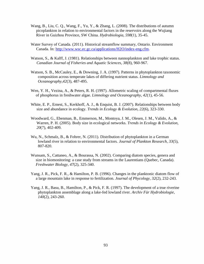
93
Wang, B., Liu, C. Q., Wang, F., Yu, Y., & Zhang, L. (2008). The distributions of autumn
picoplankton in relation to environmental factors in the reservoirs along the Wujiang
River in Guizhou Province, SW China. Hydrobiologia, 598(1), 35-45.
Water Survey of Canada. (2011). Historical streamflow summary, Ontario. Environment
Canada. In: http://www.wsc.ec.gc.ca/applications/H2O/index-eng.cfm.
Watson, S., & Kalff, J. (1981). Relationships between nannoplankton and lake trophic status.
Canadian Journal of Fisheries and Aquatic Sciences, 38(8), 960-967.
Watson, S. B., McCauley, E., & Downing, J. A. (1997). Patterns in phytoplankton taxonomic
composition across temperate lakes of differing nutrient status. Limnology and
Oceanography,42(3), 487-495.
Wen, Y. H., Vezina, A., & Peters, R. H. (1997). Allometric scaling of compartmental fluxes
of phosphorus in freshwater algae. Limnology and Oceanography, 42(1), 45-56.
White, E. P., Ernest, S., Kerkhoff, A. J., & Enquist, B. J. (2007). Relationships between body
size and abundance in ecology. Trends in Ecology & Evolution, 22(6), 323-330.
Woodward, G., Ebenman, B., Emmerson, M., Montoya, J. M., Olesen, J. M., Valido, A., &
Warren, P. H. (2005). Body size in ecological networks. Trends in Ecology & Evolution,
20(7), 402-409.
Wu, N., Schmalz, B., & Fohrer, N. (2011). Distribution of phytoplankton in a German
lowland river in relation to environmental factors. Journal of Plankton Research, 33(5),
807-820.
Wunsam, S., Cattaneo, A., & Bourassa, N. (2002). Comparing diatom species, genera and
size in biomonitoring: a case study from streams in the Laurentians (Quebec, Canada).
Freshwater Biology, 47(2), 325-340.
Yang, J. R., Pick, F. R., & Hamilton, P. B. (1996). Changes in the planktonic diatom flow of
a large mountain lake in response to fertilization. Journal of Phycology, 32(2), 232-243.
Yang, J. R., Basu, B., Hamilton, P., & Pick, F. R. (1997). The development of a true riverine
phytoplankton assemblage along a lake-fed lowland river. Archiv Für Hydrobiologie,
140(2), 243-260.
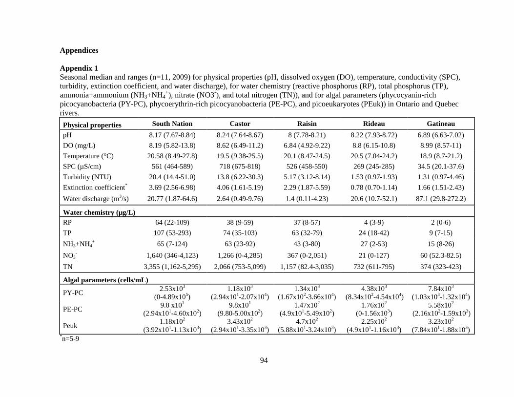
94
Appendices
Appendix 1 Seasonal median and ranges (n=11, 2009) for physical properties (pH, dissolved oxygen (DO), temperature, conductivity (SPC),
turbidity, extinction coefficient, and water discharge), for water chemistry (reactive phosphorus (RP), total phosphorus (TP),
ammonia+ammonium (NH3+NH4+), nitrate (NO3
-), and total nitrogen (TN)), and for algal parameters (phycocyanin-rich
picocyanobacteria (PY-PC), phycoerythrin-rich picocyanobacteria (PE-PC), and picoeukaryotes (PEuk)) in Ontario and Quebec
rivers.
Physical properties South Nation Castor Raisin Rideau Gatineau
pH 8.17 (7.67-8.84) 8.24 (7.64-8.67) 8 (7.78-8.21) 8.22 (7.93-8.72) 6.89 (6.63-7.02)
DO (mg/L) 8.19 (5.82-13.8) 8.62 (6.49-11.2) 6.84 (4.92-9.22) 8.8 (6.15-10.8) 8.99 (8.57-11)
Temperature (°C) 20.58 (8.49-27.8) 19.5 (9.38-25.5) 20.1 (8.47-24.5) 20.5 (7.04-24.2) 18.9 (8.7-21.2)
SPC (µS/cm) 561 (464-589) 718 (675-818) 526 (458-550) 269 (245-285) 34.5 (20.1-37.6)
Turbidity (NTU) 20.4 (14.4-51.0) 13.8 (6.22-30.3) 5.17 (3.12-8.14) 1.53 (0.97-1.93) 1.31 (0.97-4.46)
Extinction coefficient*
3.69 (2.56-6.98) 4.06 (1.61-5.19) 2.29 (1.87-5.59) 0.78 (0.70-1.14) 1.66 (1.51-2.43)
Water discharge (m3/s) 20.77 (1.87-64.6) 2.64 (0.49-9.76) 1.4 (0.11-4.23) 20.6 (10.7-52.1) 87.1 (29.8-272.2)
Water chemistry (µg/L)
RP 64 (22-109) 38 (9-59) 37 (8-57) 4 (3-9) 2 (0-6)
TP 107 (53-293) 74 (35-103) 63 (32-79) 24 (18-42) 9 (7-15)
NH3+NH4+ 65 (7-124) 63 (23-92) 43 (3-80) 27 (2-53) 15 (8-26)
NO3- 1,640 (346-4,123) 1,266 (0-4,285) 367 (0-2,051) 21 (0-127) 60 (52.3-82.5)
TN 3,355 (1,162-5,295) 2,066 (753-5,099) 1,157 (82.4-3,035) 732 (611-795) 374 (323-423)
Algal parameters (cells/mL)
PY-PC 2.53x10
3
(0-4.89x10⁵)
1.18x10³
(2.94x101-2.07x10
4)
1.34x10³
(1.67x10²-3.66x10
4)
4.38x10³
(8.34x10
2-4.54x10
4)
7.84x10³
(1.03x10³-1.32x10
4)
PE-PC 9.8 x10
1
(2.94x101-4.60x10
2)
9.8x101
(9.80-5.00x10²)
1.47x10²
(4.9x101-5.49x10
2)
1.76x10²
(0-1.56x10³)
5.58x10²
(2.16x10
2-1.59x10
3)
Peuk 1.18x10
2
(3.92x101-1.13x10
3)
3.43x10²
(2.94x101-3.35x10
3)
4.7x10²
(5.88x101-3.24x10
3)
2.25x10²
(4.9x101-1.16x10
3)
3.23x10²
(7.84x101-1.88x10
3)
*n=5-9
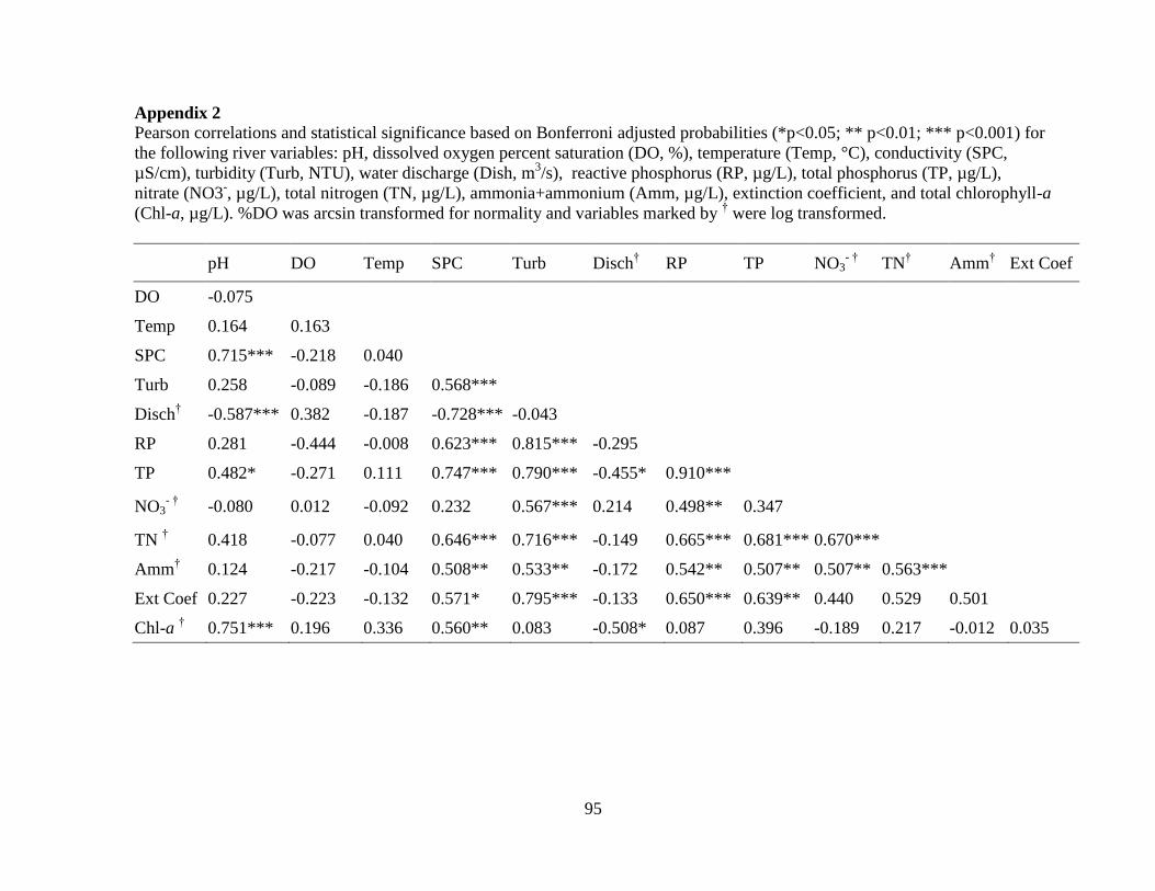
95
Appendix 2
Pearson correlations and statistical significance based on Bonferroni adjusted probabilities (*p<0.05; ** p<0.01; *** p<0.001) for
the following river variables: pH, dissolved oxygen percent saturation (DO, %), temperature (Temp, °C), conductivity (SPC,
µS/cm), turbidity (Turb, NTU), water discharge (Dish, m3/s), reactive phosphorus (RP, µg/L), total phosphorus (TP, µg/L),
nitrate (NO3-, µg/L), total nitrogen (TN, µg/L), ammonia+ammonium (Amm, µg/L), extinction coefficient, and total chlorophyll-a
(Chl-a, µg/L). %DO was arcsin transformed for normality and variables marked by † were log transformed.
pH DO Temp SPC Turb Disch
† RP TP NO3
- † TN
† Amm
† Ext Coef
DO -0.075
Temp 0.164 0.163
SPC 0.715*** -0.218 0.040
Turb 0.258 -0.089 -0.186 0.568***
Disch†
-0.587*** 0.382 -0.187 -0.728*** -0.043
RP 0.281 -0.444 -0.008 0.623*** 0.815*** -0.295
TP 0.482* -0.271 0.111 0.747*** 0.790*** -0.455* 0.910***
NO3- †
-0.080 0.012 -0.092 0.232 0.567*** 0.214 0.498** 0.347
TN † 0.418 -0.077 0.040 0.646*** 0.716*** -0.149 0.665*** 0.681*** 0.670***
Amm
† 0.124 -0.217 -0.104 0.508** 0.533** -0.172 0.542** 0.507** 0.507** 0.563***
Ext Coef 0.227 -0.223 -0.132 0.571* 0.795*** -0.133 0.650*** 0.639** 0.440 0.529 0.501
Chl-a
† 0.751*** 0.196 0.336 0.560** 0.083 -0.508* 0.087 0.396 -0.189 0.217 -0.012 0.035
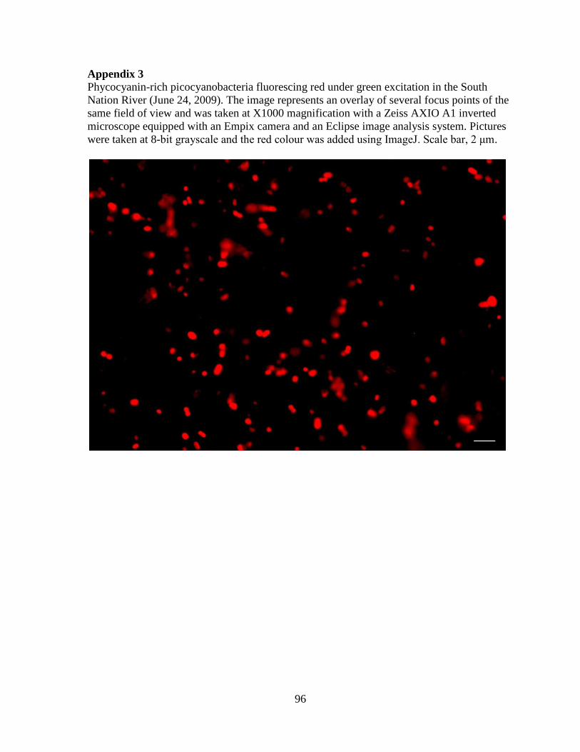
96
Appendix 3
Phycocyanin-rich picocyanobacteria fluorescing red under green excitation in the South
Nation River (June 24, 2009). The image represents an overlay of several focus points of the
same field of view and was taken at X1000 magnification with a Zeiss AXIO A1 inverted
microscope equipped with an Empix camera and an Eclipse image analysis system. Pictures
were taken at 8-bit grayscale and the red colour was added using ImageJ. Scale bar, 2 μm.
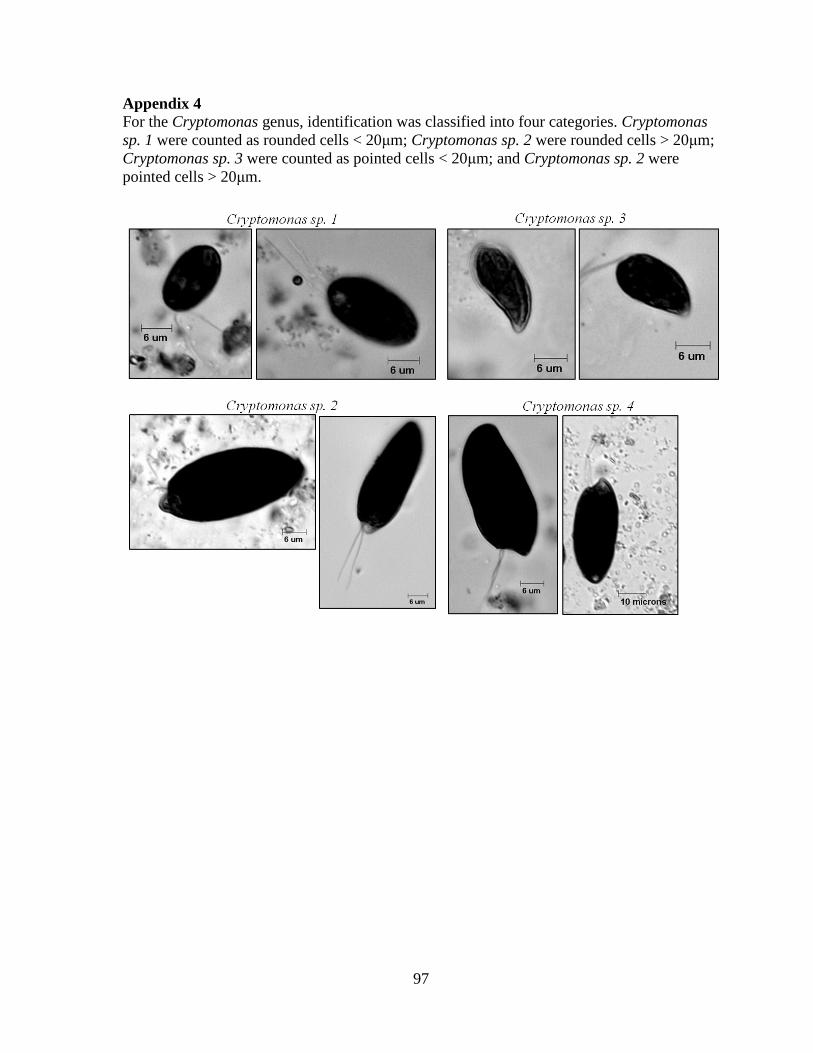
97
Appendix 4
For the Cryptomonas genus, identification was classified into four categories. Cryptomonas
sp. 1 were counted as rounded cells < 20μm; Cryptomonas sp. 2 were rounded cells > 20μm;
Cryptomonas sp. 3 were counted as pointed cells < 20μm; and Cryptomonas sp. 2 were
pointed cells > 20μm.
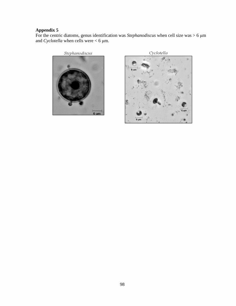
98
Appendix 5
For the centric diatoms, genus identification was Stephanodiscus when cell size was > 6 μm
and Cyclotella when cells were < 6 μm.
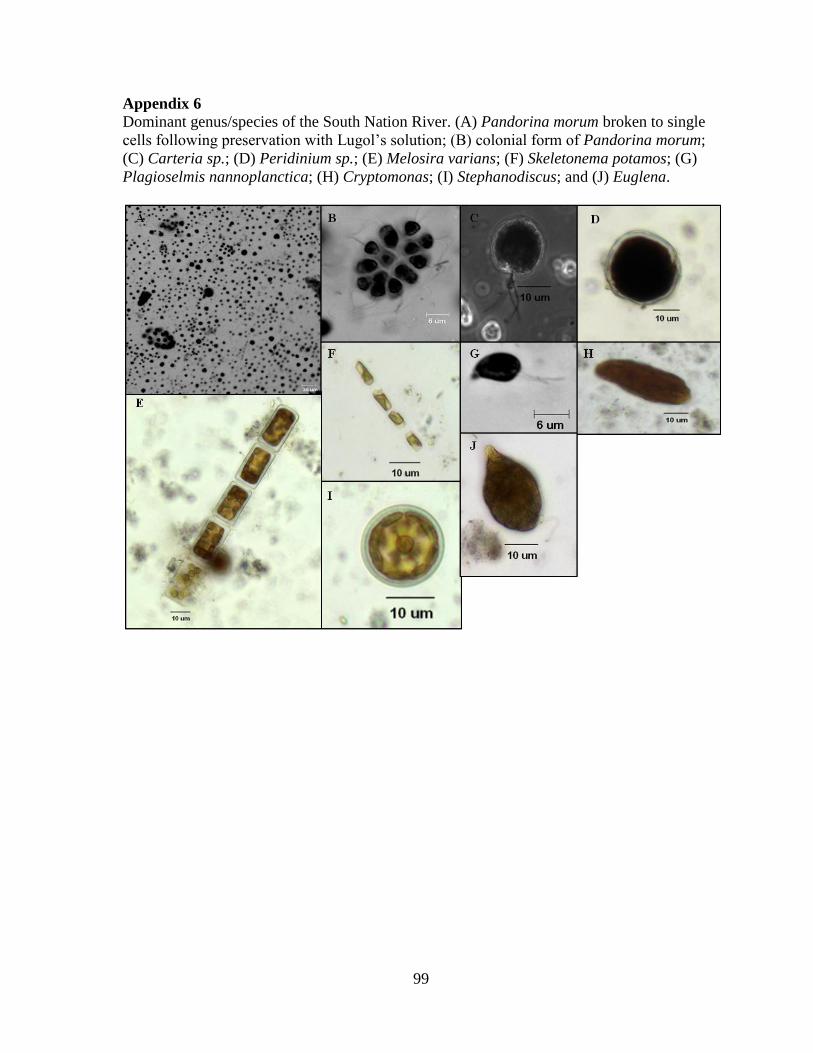
99
Appendix 6
Dominant genus/species of the South Nation River. (A) Pandorina morum broken to single
cells following preservation with Lugol’s solution; (B) colonial form of Pandorina morum;
(C) Carteria sp.; (D) Peridinium sp.; (E) Melosira varians; (F) Skeletonema potamos; (G)
Plagioselmis nannoplanctica; (H) Cryptomonas; (I) Stephanodiscus; and (J) Euglena.
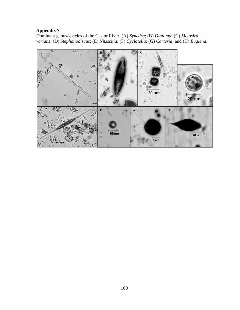
100
Appendix 7
Dominant genus/species of the Castor River. (A) Synedra; (B) Diatoma; (C) Melosira
varians; (D) Stephanodiscus; (E) Nitzschia; (F) Cyclotella; (G) Carteria; and (H) Euglena.
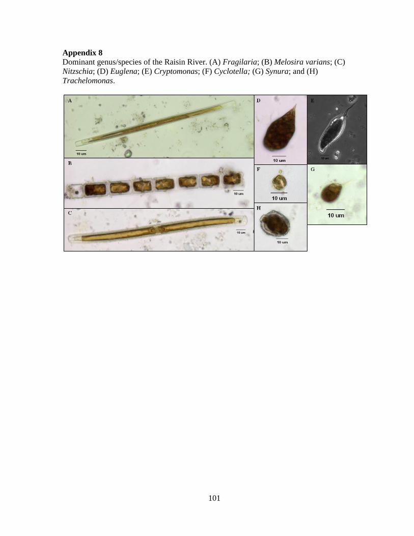
101
Appendix 8
Dominant genus/species of the Raisin River. (A) Fragilaria; (B) Melosira varians; (C)
Nitzschia; (D) Euglena; (E) Cryptomonas; (F) Cyclotella; (G) Synura; and (H)
Trachelomonas.
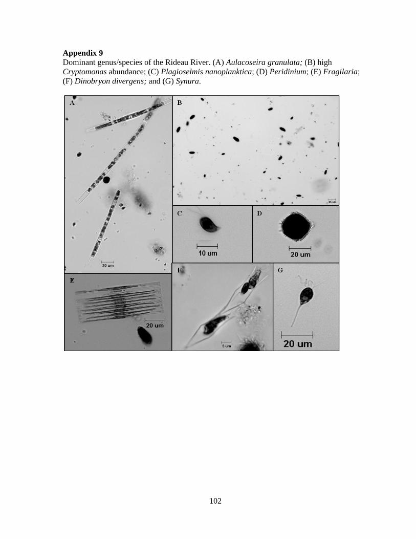
102
Appendix 9
Dominant genus/species of the Rideau River. (A) Aulacoseira granulata; (B) high
Cryptomonas abundance; (C) Plagioselmis nanoplanktica; (D) Peridinium; (E) Fragilaria;
(F) Dinobryon divergens; and (G) Synura.
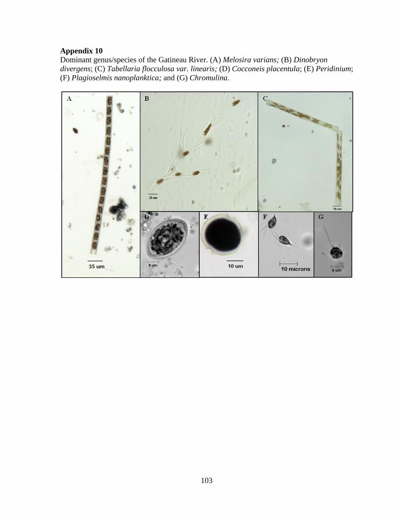
103
Appendix 10
Dominant genus/species of the Gatineau River. (A) Melosira varians; (B) Dinobryon
divergens; (C) Tabellaria flocculosa var. linearis; (D) Cocconeis placentula; (E) Peridinium;
(F) Plagioselmis nanoplanktica; and (G) Chromulina.
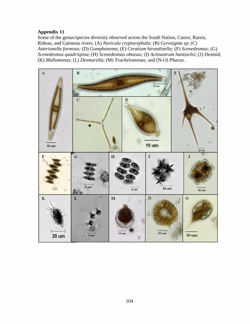
104
Appendix 11
Some of the genus/species diversity observed across the South Nation, Castor, Raisin,
Rideau, and Gatineau rivers. (A) Navicula cryptocephala; (B) Gyrosigma sp; (C)
Asterionella formosa; (D) Gomphonema; (E) Ceratium hirundinella; (F) Scenedesmus; (G)
Scenedesmus quadrispina; (H) Scenedesmus obtusus; (I) Actinastrum hantzschii; (J) Desmid;
(K) Mallomonas; (L) Desmarella; (M) Trachelomonas; and (N-O) Phacus.
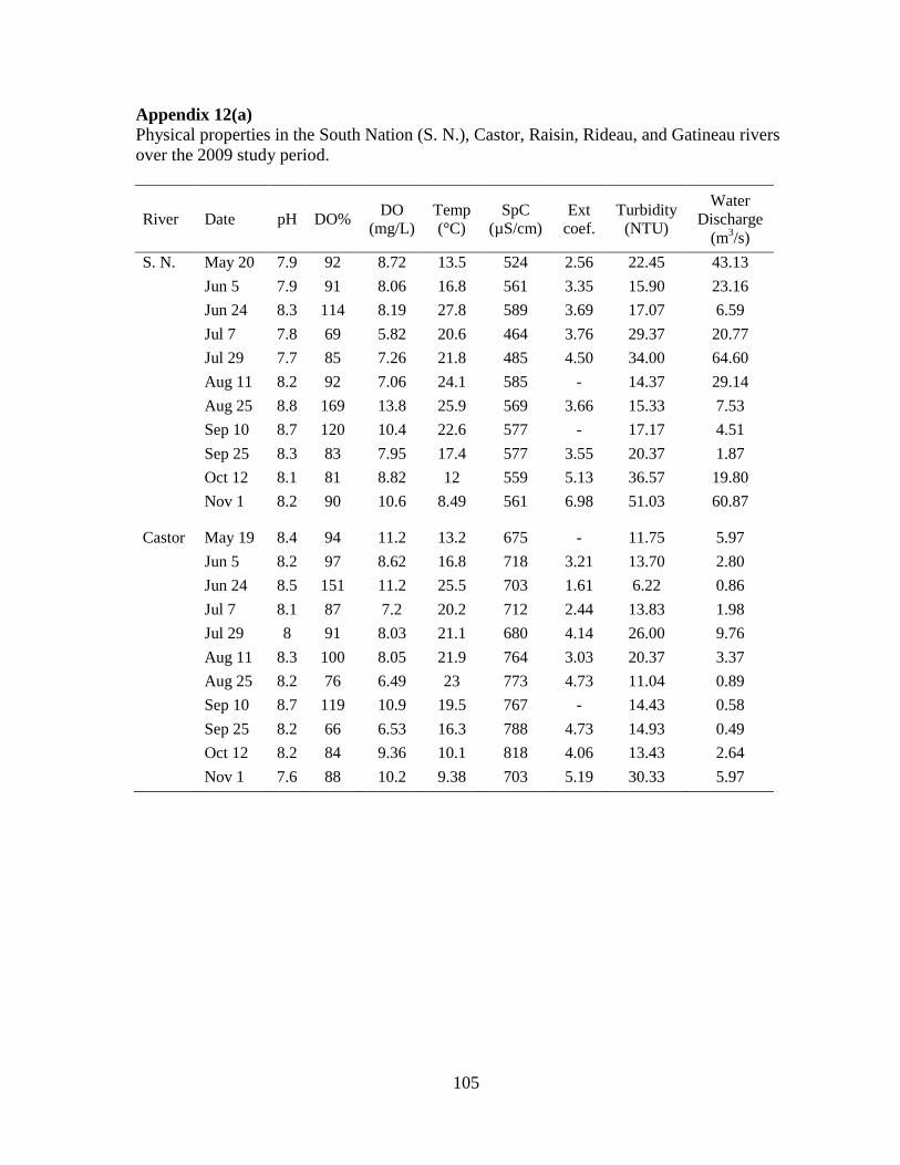
105
Appendix 12(a)
Physical properties in the South Nation (S. N.), Castor, Raisin, Rideau, and Gatineau rivers
over the 2009 study period.
River Date pH DO% DO
(mg/L)
Temp
(°C)
SpC
(µS/cm)
Ext
coef.
Turbidity
(NTU)
Water
Discharge
(m3/s)
S. N. May 20 7.9 92 8.72 13.5 524 2.56 22.45 43.13
Jun 5 7.9 91 8.06 16.8 561 3.35 15.90 23.16
Jun 24 8.3 114 8.19 27.8 589 3.69 17.07 6.59
Jul 7 7.8 69 5.82 20.6 464 3.76 29.37 20.77
Jul 29 7.7 85 7.26 21.8 485 4.50 34.00 64.60
Aug 11 8.2 92 7.06 24.1 585 - 14.37 29.14
Aug 25 8.8 169 13.8 25.9 569 3.66 15.33 7.53
Sep 10 8.7 120 10.4 22.6 577 - 17.17 4.51
Sep 25 8.3 83 7.95 17.4 577 3.55 20.37 1.87
Oct 12 8.1 81 8.82 12 559 5.13 36.57 19.80
Nov 1 8.2 90 10.6 8.49 561 6.98 51.03 60.87
Castor May 19 8.4 94 11.2 13.2 675 - 11.75 5.97
Jun 5 8.2 97 8.62 16.8 718 3.21 13.70 2.80
Jun 24 8.5 151 11.2 25.5 703 1.61 6.22 0.86
Jul 7 8.1 87 7.2 20.2 712 2.44 13.83 1.98
Jul 29 8 91 8.03 21.1 680 4.14 26.00 9.76
Aug 11 8.3 100 8.05 21.9 764 3.03 20.37 3.37
Aug 25 8.2 76 6.49 23 773 4.73 11.04 0.89
Sep 10 8.7 119 10.9 19.5 767 - 14.43 0.58
Sep 25 8.2 66 6.53 16.3 788 4.73 14.93 0.49
Oct 12 8.2 84 9.36 10.1 818 4.06 13.43 2.64
Nov 1 7.6 88 10.2 9.38 703 5.19 30.33 5.97
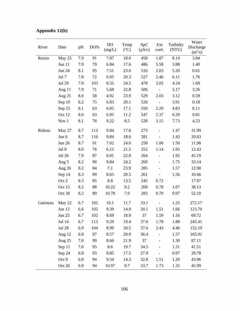
106
Appendix 12(b)
River Date pH DO% DO
(mg/L)
Temp
(°C)
SpC
(µS/c)
Ext
coef.
Turbidiy
(NTU)
Water
Discharge
(m3/s)
Raisin May 25 7.9 91 7.87 18.0 458 1.87 8.14 3.84
Jun 11 7.9 79 6.84 17.6 486 5.58 3.88 1.40
Jun 24 8.1 95 7.51 23.6 516 2.03 5.20 0.61
Jul 7 7.8 72 6.05 20.3 527 2.46 6.11 1.76
Jul 29 7.9 103 8.55 24.5 478 2.02 4.24 1.69
Aug 11 7.9 71 5.68 22.8 506 - 5.17 3.26
Aug 25 8.0 58 4.92 23.9 529 2.03 3.12 0.59
Sep 10 8.2 75 6.83 20.1 526 - 3.91 0.18
Sep 25 8.1 63 6.05 17.1 550 2.29 4.83 0.11
Oct 12 8.0 63 6.95 11.2 547 2.37 6.29 0.81
Nov 1 8.1 78 9.22 8.5 528 3.15 7.73 4.23
Rideau May 27 8.7 113 9.84 17.6 273 - 1.47 31.99
Jun 6 8.7 116 9.84 18.6 281 - 1.43 20.63
Jun 26 8.7 91 7.02 24.0 258 1.06 1.50 11.98
Jul 8 8.0 76 6.15 21.5 252 1.14 1.93 12.43
Jul 26 7.9 87 6.81 22.8 264 - 1.92 45.19
Aug 5 8.2 90 9.84 24.2 269 - 1.75 33.14
Aug 26 8.2 84 7.1 23.9 285 - 1.57 12.90
Sep 14 8.3 89 8.65 20.5 261 - 1.56 10.66
Oct 2 8.3 85 8.8 13.5 245 0.72 17.97
Oct 15 8.2 88 10.22 9.2 269 0.78 1.07 38.13
Oct 30 8.2 89 10.78 7.0 283 0.70 0.97 52.10
Gatineau May 22 6.7 102 10.1 11.7 33.1 - 1.25 272.17
Jun 12 6.6 102 9.39 14.9 20.1 1.51 1.66 123.70
Jun 25 6.7 102 8.69 18.9 37 1.59 1.16 69.72
Jul 14 6.7 113 9.29 19.4 37.6 1.78 1.88 245.41
Jul 28 6.9 104 8.99 20.5 37.6 2.43 4.46 152.19
Aug 12 6.9 97 8.57 20.9 36.4 - 1.57 165.01
Aug 25 7.0 99 8.66 21.9 37 - 1.30 87.11
Sep 11 7.0 95 8.6 19.7 34.5 - 1.31 41.51
Sep 24 6.9 93 8.85 17.5 27.9 - 0.97 29.78
Oct 9 6.8 94 9.54 14.3 32.8 1.51 1.20 43.96
Oct 26 6.9 94 10.97 8.7 33.7 1.73 1.35 45.99
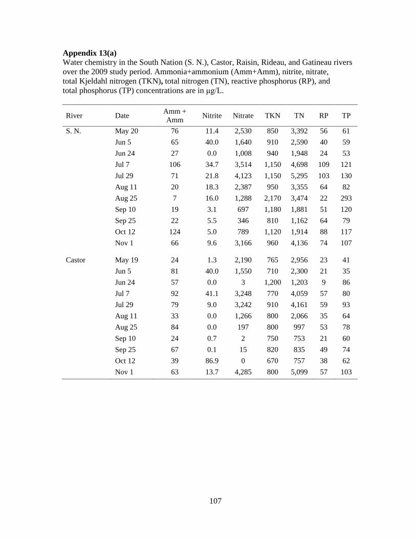
107
Appendix 13(a)
Water chemistry in the South Nation (S. N.), Castor, Raisin, Rideau, and Gatineau rivers
over the 2009 study period. Ammonia+ammonium (Amm+Amm), nitrite, nitrate,
total Kjeldahl nitrogen (TKN), total nitrogen (TN), reactive phosphorus (RP), and
total phosphorus (TP) concentrations are in μg/L.
River Date Amm +
Amm Nitrite Nitrate TKN TN RP TP
S. N. May 20 76 11.4 2,530 850 3,392 56 61
Jun 5 65 40.0 1,640 910 2,590 40 59
Jun 24 27 0.0 1,008 940 1,948 24 53
Jul 7 106 34.7 3,514 1,150 4,698 109 121
Jul 29 71 21.8 4,123 1,150 5,295 103 130
Aug 11 20 18.3 2,387 950 3,355 64 82
Aug 25 7 16.0 1,288 2,170 3,474 22 293
Sep 10 19 3.1 697 1,180 1,881 51 120
Sep 25 22 5.5 346 810 1,162 64 79
Oct 12 124 5.0 789 1,120 1,914 88 117
Nov 1 66 9.6 3,166 960 4,136 74 107
Castor May 19 24 1.3 2,190 765 2,956 23 41
Jun 5 81 40.0 1,550 710 2,300 21 35
Jun 24 57 0.0 3 1,200 1,203 9 86
Jul 7 92 41.1 3,248 770 4,059 57 80
Jul 29 79 9.0 3,242 910 4,161 59 93
Aug 11 33 0.0 1,266 800 2,066 35 64
Aug 25 84 0.0 197 800 997 53 78
Sep 10 24 0.7 2 750 753 21 60
Sep 25 67 0.1 15 820 835 49 74
Oct 12 39 86.9 0 670 757 38 62
Nov 1 63 13.7 4,285 800 5,099 57 103
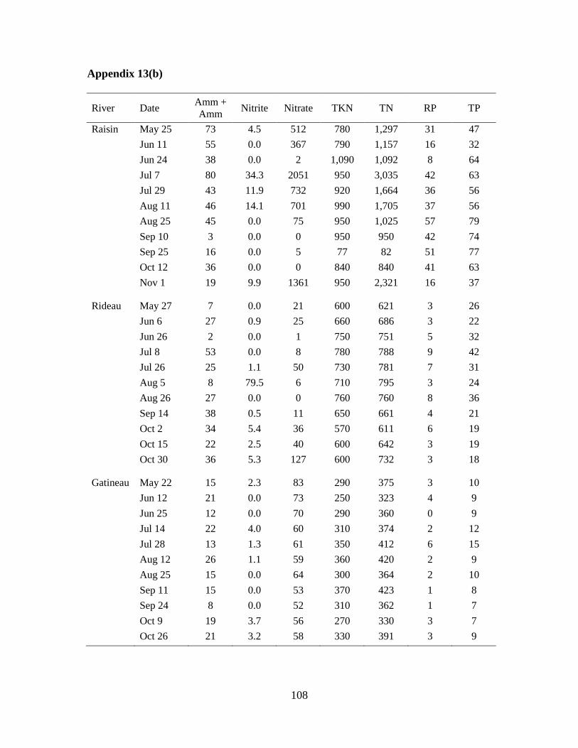
108
Appendix 13(b)
River Date Amm +
Amm Nitrite Nitrate TKN TN RP TP
Raisin May 25 73 4.5 512 780 1,297 31 47
Jun 11 55 0.0 367 790 1,157 16 32
Jun 24 38 0.0 2 1,090 1,092 8 64
Jul 7 80 34.3 2051 950 3,035 42 63
Jul 29 43 11.9 732 920 1,664 36 56
Aug 11 46 14.1 701 990 1,705 37 56
Aug 25 45 0.0 75 950 1,025 57 79
Sep 10 3 0.0 0 950 950 42 74
Sep 25 16 0.0 5 77 82 51 77
Oct 12 36 0.0 0 840 840 41 63
Nov 1 19 9.9 1361 950 2,321 16 37
Rideau May 27 7 0.0 21 600 621 3 26
Jun 6 27 0.9 25 660 686 3 22
Jun 26 2 0.0 1 750 751 5 32
Jul 8 53 0.0 8 780 788 9 42
Jul 26 25 1.1 50 730 781 7 31
Aug 5 8 79.5 6 710 795 3 24
Aug 26 27 0.0 0 760 760 8 36
Sep 14 38 0.5 11 650 661 4 21
Oct 2 34 5.4 36 570 611 6 19
Oct 15 22 2.5 40 600 642 3 19
Oct 30 36 5.3 127 600 732 3 18
Gatineau May 22 15 2.3 83 290 375 3 10
Jun 12 21 0.0 73 250 323 4 9
Jun 25 12 0.0 70 290 360 0 9
Jul 14 22 4.0 60 310 374 2 12
Jul 28 13 1.3 61 350 412 6 15
Aug 12 26 1.1 59 360 420 2 9
Aug 25 15 0.0 64 300 364 2 10
Sep 11 15 0.0 53 370 423 1 8
Sep 24 8 0.0 52 310 362 1 7
Oct 9 19 3.7 56 270 330 3 7
Oct 26 21 3.2 58 330 391 3 9
109
Appendix 14(a)
Total picophytoplankton abundance for each pigment group in the South Nation (S. N.),
Castor, Raisin, Rideau, and Gatineau rivers over the 2009 study period. Phycocyanin-rich
picocyanobacteria (PY-PC), phycoerythrin-rich picocyanobacteria (PE-PC), and
picoeukaryotes (PEuk) values are in cells/mL.
River Date PY-PC PE-PC PEuk
S. N. May 20 0.00E+00 2.25E+02 3.92E+01
Jun 5 2.65E+02 1.47E+02 4.90E+01
Jun 24 4.89E+05 4.60E+02 1.13E+03
Jul 7 8.56E+03 8.82E+01 5.29E+02
Jul 29 1.03E+03 6.86E+01 1.67E+02
Aug 11 2.53E+03 1.08E+02 6.86E+01
Aug 25 1.72E+04 9.80E+01 2.06E+02
Sep 10 1.14E+04 2.94E+01 1.18E+02
Sep 25 5.54E+03 8.82E+01 7.84E+01
Oct 12 6.66E+02 5.88E+01 1.08E+02
Nov 1 2.65E+02 1.47E+02 1.18E+02
Castor May 19 2.94E+01 5.88E+01 2.94E+01
Jun 5 4.31E+02 1.57E+02 1.86E+02
Jun 24 1.58E+03 4.90E+01 1.20E+03
Jul 7 1.09E+03 1.27E+02 3.35E+03
Jul 29 1.18E+03 8.82E+01 7.84E+01
Aug 11 5.15E+03 9.80E+01 4.90E+02
Aug 25 2.75E+03 1.27E+02 1.73E+03
Sep 10 2.07E+04 6.86E+01 2.70E+03
Sep 25 1.57E+03 9.80E+00 3.43E+02
Oct 12 9.80E+01 5.00E+02 1.76E+02
Nov 1 1.18E+02 2.45E+02 2.16E+02
110
Appendix 14(b)
River Date PY-PC PE-PC PEuk
Raisin May 25 5.68E+02 4.90E+01 5.88E+01
Jun 11 4.11E+02 6.86E+01 1.18E+02
Jun 24 9.82E+03 1.86E+02 1.50E+03
Jul 7 1.43E+03 1.47E+02 1.80E+03
Jul 29 1.34E+03 8.82E+01 3.43E+02
Aug 11 9.99E+02 1.37E+02 2.55E+02
Aug 25 2.01E+04 5.49E+02 1.42E+03
Sep 10 3.66E+04 3.82E+02 1.47E+03
Sep 25 1.03E+04 1.18E+02 3.24E+03
Oct 12 5.39E+02 2.35E+02 4.70E+02
Nov 1 1.67E+02 2.94E+02 7.84E+01
Rideau May 27 1.54E+03 9.80E+00 5.58E+02
Jun 6 1.64E+03 1.96E+01 4.90E+02
Jun 26 4.38E+03 6.86E+01 8.82E+01
Jul 8 3.34E+04 2.74E+02 6.07E+02
Jul 26 3.70E+04 3.43E+02 1.16E+03
Aug 5 2.45E+04 1.08E+03 2.35E+02
Aug 26 4.54E+04 1.11E+03 2.06E+02
Sep 14 2.42E+04 1.56E+03 8.82E+01
Oct 2 2.80E+03 1.76E+02 2.25E+02
Oct 15 8.41E+02 0.00E+00 8.82E+01
Oct 30 8.34E+02 6.86E+01 4.90E+01
Gatineau May 22 1.03E+03 5.58E+02 7.84E+01
Jun 12 2.38E+03 7.05E+02 1.08E+02
Jun 25 6.96E+03 8.33E+02 1.88E+03
Jul 14 1.32E+04 1.59E+03 7.84E+02
Jul 28 1.20E+04 8.23E+02 4.02E+02
Aug 12 1.14E+04 5.98E+02 3.13E+02
Aug 25 7.84E+03 3.62E+02 4.70E+02
Sep 11 1.29E+04 3.23E+02 3.13E+02
Sep 24 9.49E+03 2.16E+02 2.94E+02
Oct 9 7.55E+03 3.04E+02 3.23E+02
Oct 26 6.25E+03 3.33E+02 3.92E+02
111
Appendix 15(a)
Chlorophyll-a (Chl-a) and biomass from microscope enumerations in the South Nation
(S. N.), Castor, Raisin, Rideau, and Gatineau rivers over the 2009 study period. Total values
and those for larger cells (> 2 μm) and picophytoplankton (< 2 μm) are in μg/L. The relative
abundance of picophytoplankton is also represented (%PP) for both chl-a and biomass from
enumerations.
Chl-a Biomass
River Date Total > 2 μm
< 2
μm % PP Total
> 2
μm
< 2
μm % PP
S. N. May 20 1.70 1.55 0.15 8.82 831 831 0.14 0.02
Jun 5 1.48 0.22 1.26 85.14 609 608 0.24 0.04
Jun 24 - - - - 2,838 2,582 256 9.05
Jul 7 1.14 0.72 0.42 36.84 502 498 4.81 0.96
Jul 29 - - - - 490 489 0.66 0.14
Aug 11 3.66 2.87 0.79 21.58 689 687 1.42 0.21
Aug 25 126.49 84.13 42.36 33.49 38,221 38,212 9.15 0.02
Sep 10 18.64 8.82 9.82 52.68 3,653 3,647 6.05 0.17
Sep 25 8.17 1.85 6.32 77.36 964 961 2.99 0.31
Oct 12 1.60 0.75 0.85 53.13 271 271 0.44 0.16
Nov 1 2.06 1.20 0.86 41.75 348 347 0.28 0.08
Castor May 19 8.10 6.59 1.51 18.64 2,523 2,523 0.06 0.00
Jun 5 - - - - 1,141 1,141 0.41 0.04
Jun 24 19.28 17.06 2.22 11.51 5,397 5,396 1.48 0.03
Jul 7 2.94 2.27 0.67 22.79 1,774 1,772 2.39 0.13
Jul 29 1.54 2.61 0.00 0.00 1,146 1,146 0.70 0.06
Aug 11 5.23 4.34 0.89 17.02 1,358 1,355 3.01 0.22
Aug 25 6.18 1.97 4.21 68.12 3,837 3,835 2.42 0.06
Sep 10 11.66 10.66 1.00 8.58 4,965 4,952 12.26 0.25
Sep 25 8.32 2.08 6.24 75.00 1,812 1,811 1.01 0.06
Oct 12 1.61 2.05 0.00 0.00 1,103 1,102 0.41 0.04
Nov 1 3.46 2.23 1.23 35.55 2,506 2,506 0.30 0.01
112
Appendix 15(b)
Chl-a Biomass
River Date Total > 2
μm
< 2
μm % PP Total
> 2
μm
< 2
μm % PP
Raisin May 25 1.47 1.02 0.45 30.61 867 866 0.35 0.04
Jun 11 2.63 2.19 0.44 16.73 305 304 0.31 0.10
Jun 24 14.07 9.96 4.11 29.21 3,377 3,371 6.02 0.18
Jul 7 3.22 3.14 0.08 2.48 3,545 3,543 1.77 0.05
Jul 29 3.58 1.94 1.64 45.81 1,105 1,104 0.93 0.08
Aug 11 1.69 1.67 0.02 1.18 714 713 0.73 0.10
Aug 25 2.13 2.42 0.00 0.00 849 838 11.54 1.36
Sep 10 3.19 4.94 0.00 0.00 1,255 1,235 20.15 1.61
Sep 25 2.88 2.43 0.45 15.63 1,877 1,870 7.18 0.38
Oct 12 1.96 0.87 1.09 55.61 474 473 0.65 0.14
Nov 1 1.22 1.93 0.00 0.00 589 589 0.28 0.05
Rideau May 27 5.37 4.00 1.37 25.51 1,549 1,548 1.10 0.07
Jun 6 3.14 2.34 0.80 25.48 3,435 3,434 1.12 0.03
Jun 26 5.58 5.01 0.57 10.22 2,190 2,187 2.38 0.11
Jul 8 - - - - 26,547 26,529 17.97 0.07
Jul 26 6.28 4.73 1.55 24.68 2,435 2,415 20.17 0.83
Aug 5 9.89 6.41 3.48 35.19 2,592 2,579 13.52 0.52
Aug 26 4.67 5.00 0.00 0.00 2,735 2,711 24.47 0.89
Sep 14 1.97 1.35 0.62 31.47 - - - -
Oct 2 3.14 2.11 1.03 32.80 1,433 1,431 1.68 0.12
Oct 15 2.07 0.96 1.11 53.62 1,150 1,150 0.49 0.04
Oct 30 2.34 1.00 1.34 57.26 744 743 0.50 0.07
Gatineau May 22 - - - - 296 295 0.87 0.29
Jun 12 - - - - 342 340 1.67 0.49
Jun 25 1.01 1.13 0.00 0.00 413 408 5.06 1.23
Jul 14 1.14 0.85 0.29 25.44 303 295 8.14 2.69
Jul 28 0.97 0.74 0.23 23.71 182 175 6.95 3.81
Aug 12 0.95 0.57 0.38 40.00 120 114 6.44 5.36
Aug 25 0.56 0.52 0.04 7.14 274 269 4.54 1.66
Sep 11 0.45 0.50 0.00 0.00 371 364 7.07 1.91
Sep 24 0.68 0.47 0.21 30.88 205 199 5.24 2.56
Oct 9 - - - - 143 139 4.28 2.99
Oct 26 0.76 0.00 0.00 3.65 191 188 3.65 1.91
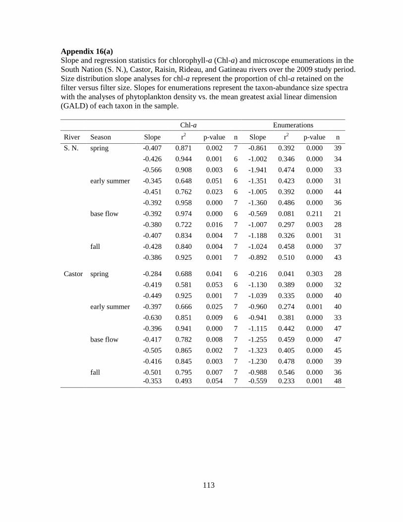
113
Appendix 16(a)
Slope and regression statistics for chlorophyll-a (Chl-a) and microscope enumerations in the
South Nation (S. N.), Castor, Raisin, Rideau, and Gatineau rivers over the 2009 study period.
Size distribution slope analyses for chl-a represent the proportion of chl-a retained on the
filter versus filter size. Slopes for enumerations represent the taxon-abundance size spectra
with the analyses of phytoplankton density vs. the mean greatest axial linear dimension
(GALD) of each taxon in the sample.
Chl-a Enumerations
River Season Slope r2 p-value n Slope r
2 p-value n
S. N. spring -0.407 0.871 0.002 7 -0.861 0.392 0.000 39
-0.426 0.944 0.001 6 -1.002 0.346 0.000 34
-0.566 0.908 0.003 6 -1.941 0.474 0.000 33
early summer -0.345 0.648 0.051 6 -1.351 0.423 0.000 31
-0.451 0.762 0.023 6 -1.005 0.392 0.000 44
-0.392 0.958 0.000 7 -1.360 0.486 0.000 36
base flow -0.392 0.974 0.000 6 -0.569 0.081 0.211 21
-0.380 0.722 0.016 7 -1.007 0.297 0.003 28
-0.407 0.834 0.004 7 -1.188 0.326 0.001 31
fall -0.428 0.840 0.004 7 -1.024 0.458 0.000 37
-0.386 0.925 0.001 7 -0.892 0.510 0.000 43
Castor spring -0.284 0.688 0.041 6 -0.216 0.041 0.303 28
-0.419 0.581 0.053 6 -1.130 0.389 0.000 32
-0.449 0.925 0.001 7 -1.039 0.335 0.000 40
early summer -0.397 0.666 0.025 7 -0.960 0.274 0.001 40
-0.630 0.851 0.009 6 -0.941 0.381 0.000 33
-0.396 0.941 0.000 7 -1.115 0.442 0.000 47
base flow -0.417 0.782 0.008 7 -1.255 0.459 0.000 47
-0.505 0.865 0.002 7 -1.323 0.405 0.000 45
-0.416 0.845 0.003 7 -1.230 0.478 0.000 39
fall -0.501 0.795 0.007 7 -0.988 0.546 0.000 36
-0.353 0.493 0.054 7 -0.559 0.233 0.001 48
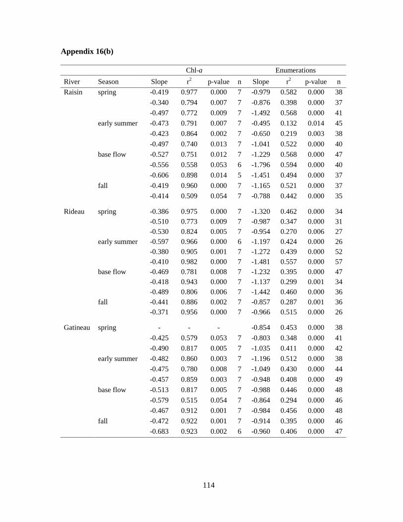
114
Appendix 16(b)
Chl-a Enumerations
River Season Slope r2 p-value n Slope r
2 p-value n
Raisin spring -0.419 0.977 0.000 7 -0.979 0.582 0.000 38
-0.340 0.794 0.007 7 -0.876 0.398 0.000 37
-0.497 0.772 0.009 7 -1.492 0.568 0.000 41
early summer -0.473 0.791 0.007 7 -0.495 0.132 0.014 45
-0.423 0.864 0.002 7 -0.650 0.219 0.003 38
-0.497 0.740 0.013 7 -1.041 0.522 0.000 40
base flow -0.527 0.751 0.012 7 -1.229 0.568 0.000 47
-0.556 0.558 0.053 6 -1.796 0.594 0.000 40
-0.606 0.898 0.014 5 -1.451 0.494 0.000 37
fall -0.419 0.960 0.000 7 -1.165 0.521 0.000 37
-0.414 0.509 0.054 7 -0.788 0.442 0.000 35
Rideau spring -0.386 0.975 0.000 7 -1.320 0.462 0.000 34
-0.510 0.773 0.009 7 -0.987 0.347 0.000 31
-0.530 0.824 0.005 7 -0.954 0.270 0.006 27
early summer -0.597 0.966 0.000 6 -1.197 0.424 0.000 26
-0.380 0.905 0.001 7 -1.272 0.439 0.000 52
-0.410 0.982 0.000 7 -1.481 0.557 0.000 57
base flow -0.469 0.781 0.008 7 -1.232 0.395 0.000 47
-0.418 0.943 0.000 7 -1.137 0.299 0.001 34
-0.489 0.806 0.006 7 -1.442 0.460 0.000 36
fall -0.441 0.886 0.002 7 -0.857 0.287 0.001 36
-0.371 0.956 0.000 7 -0.966 0.515 0.000 26
Gatineau spring - - - -0.854 0.453 0.000 38
-0.425 0.579 0.053 7 -0.803 0.348 0.000 41
-0.490 0.817 0.005 7 -1.035 0.411 0.000 42
early summer -0.482 0.860 0.003 7 -1.196 0.512 0.000 38
-0.475 0.780 0.008 7 -1.049 0.430 0.000 44
-0.457 0.859 0.003 7 -0.948 0.408 0.000 49
base flow -0.513 0.817 0.005 7 -0.988 0.446 0.000 48
-0.579 0.515 0.054 7 -0.864 0.294 0.000 46
-0.467 0.912 0.001 7 -0.984 0.456 0.000 48
fall -0.472 0.922 0.001 7 -0.914 0.395 0.000 46
-0.683 0.923 0.002 6 -0.960 0.406 0.000 47
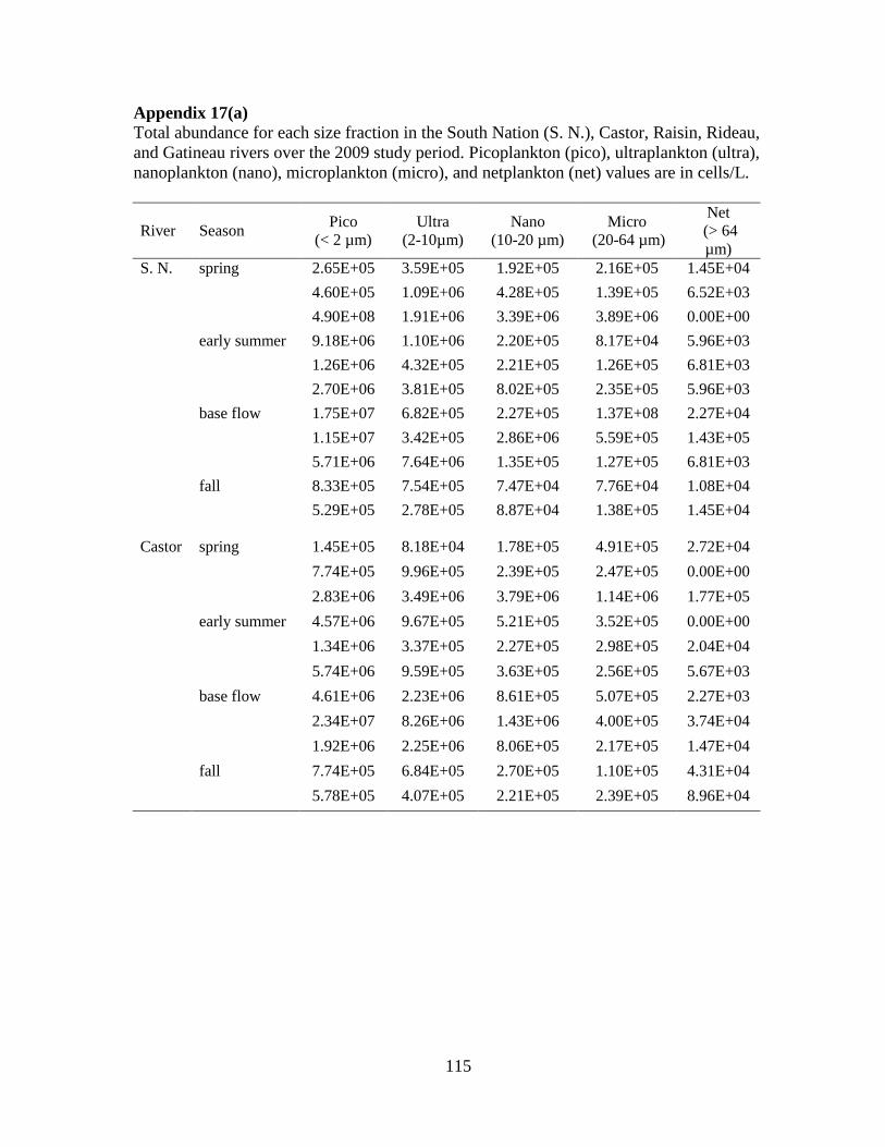
115
Appendix 17(a)
Total abundance for each size fraction in the South Nation (S. N.), Castor, Raisin, Rideau,
and Gatineau rivers over the 2009 study period. Picoplankton (pico), ultraplankton (ultra),
nanoplankton (nano), microplankton (micro), and netplankton (net) values are in cells/L.
River Season Pico
(< 2 µm)
Ultra
(2-10µm)
Nano
(10-20 µm)
Micro
(20-64 µm)
Net
(> 64
µm)
S. N. spring 2.65E+05 3.59E+05 1.92E+05 2.16E+05 1.45E+04
4.60E+05 1.09E+06 4.28E+05 1.39E+05 6.52E+03
4.90E+08 1.91E+06 3.39E+06 3.89E+06 0.00E+00
early summer 9.18E+06 1.10E+06 2.20E+05 8.17E+04 5.96E+03
1.26E+06 4.32E+05 2.21E+05 1.26E+05 6.81E+03
2.70E+06 3.81E+05 8.02E+05 2.35E+05 5.96E+03
base flow 1.75E+07 6.82E+05 2.27E+05 1.37E+08 2.27E+04
1.15E+07 3.42E+05 2.86E+06 5.59E+05 1.43E+05
5.71E+06 7.64E+06 1.35E+05 1.27E+05 6.81E+03
fall 8.33E+05 7.54E+05 7.47E+04 7.76E+04 1.08E+04
5.29E+05 2.78E+05 8.87E+04 1.38E+05 1.45E+04
Castor spring 1.45E+05 8.18E+04 1.78E+05 4.91E+05 2.72E+04
7.74E+05 9.96E+05 2.39E+05 2.47E+05 0.00E+00
2.83E+06 3.49E+06 3.79E+06 1.14E+06 1.77E+05
early summer 4.57E+06 9.67E+05 5.21E+05 3.52E+05 0.00E+00
1.34E+06 3.37E+05 2.27E+05 2.98E+05 2.04E+04
5.74E+06 9.59E+05 3.63E+05 2.56E+05 5.67E+03
base flow 4.61E+06 2.23E+06 8.61E+05 5.07E+05 2.27E+03
2.34E+07 8.26E+06 1.43E+06 4.00E+05 3.74E+04
1.92E+06 2.25E+06 8.06E+05 2.17E+05 1.47E+04
fall 7.74E+05 6.84E+05 2.70E+05 1.10E+05 4.31E+04
5.78E+05 4.07E+05 2.21E+05 2.39E+05 8.96E+04
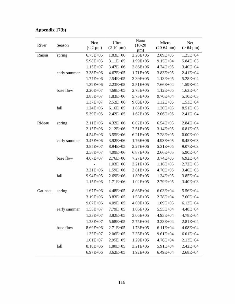
116
Appendix 17(b)
River Season Pico
(< 2 µm)
Ultra
(2-10 µm)
Nano
(10-20
µm)
Micro
(20-64 µm)
Net
(> 64 µm)
Raisin spring 6.75E+05 1.83E+06 2.28E+05 2.89E+05 1.25E+04
5.98E+05 3.11E+05 1.99E+05 9.15E+04 5.84E+03
1.15E+07 3.47E+06 2.86E+06 4.74E+05 3.40E+04
early summer 3.38E+06 4.67E+05 1.71E+05 3.83E+05 2.41E+04
1.77E+06 2.54E+05 3.39E+05 1.13E+05 5.28E+04
1.39E+06 2.23E+05 2.51E+05 7.66E+04 1.59E+04
base flow 2.20E+07 4.68E+05 2.73E+05 1.12E+05 1.63E+04
3.85E+07 1.83E+06 5.73E+05 9.70E+04 5.10E+03
1.37E+07 2.52E+06 9.08E+05 1.32E+05 1.53E+04
fall 1.24E+06 6.16E+05 1.88E+05 1.30E+05 8.51E+03
5.39E+05 2.42E+05 1.62E+05 2.06E+05 2.41E+04
Rideau spring 2.11E+06 4.32E+06 6.02E+05 6.54E+05 2.84E+04
2.15E+06 2.12E+06 2.51E+05 3.14E+05 6.81E+03
4.54E+06 3.55E+06 6.21E+05 7.28E+05 0.00E+00
early summer 3.45E+06 3.92E+06 1.76E+06 4.93E+05 8.45E+03
3.85E+07 8.94E+05 2.27E+06 5.31E+05 9.07E+03
2.58E+07 4.09E+06 6.87E+05 2.66E+05 5.90E+04
base flow 4.67E+07 2.76E+06 7.27E+05 3.74E+05 6.92E+04
- 1.03E+06 3.21E+05 1.16E+05 2.72E+03
3.21E+06 1.59E+06 2.81E+05 4.70E+05 3.40E+03
fall 9.94E+05 2.69E+06 1.89E+05 1.34E+05 3.85E+04
1.15E+06 1.71E+06 1.02E+05 2.79E+05 3.40E+03
Gatineau spring 1.67E+06 4.48E+05 8.66E+04 6.03E+04 5.56E+04
3.19E+06 3.83E+05 1.53E+05 2.78E+04 7.60E+04
9.67E+06 4.09E+05 4.00E+05 1.09E+05 6.13E+04
early summer 1.55E+07 7.79E+05 1.06E+05 5.55E+04 4.48E+04
1.33E+07 3.82E+05 3.06E+05 4.93E+04 4.78E+04
1.23E+07 5.68E+05 2.75E+04 3.33E+04 2.81E+04
base flow 8.69E+06 2.71E+05 1.73E+05 6.11E+04 4.08E+04
1.35E+07 2.06E+05 2.35E+05 9.61E+04 6.01E+04
1.01E+07 2.95E+05 1.29E+05 4.76E+04 2.13E+04
fall 8.18E+06 1.80E+05 3.21E+05 5.91E+04 2.42E+04
6.97E+06 3.62E+05 1.92E+05 6.49E+04 2.68E+04
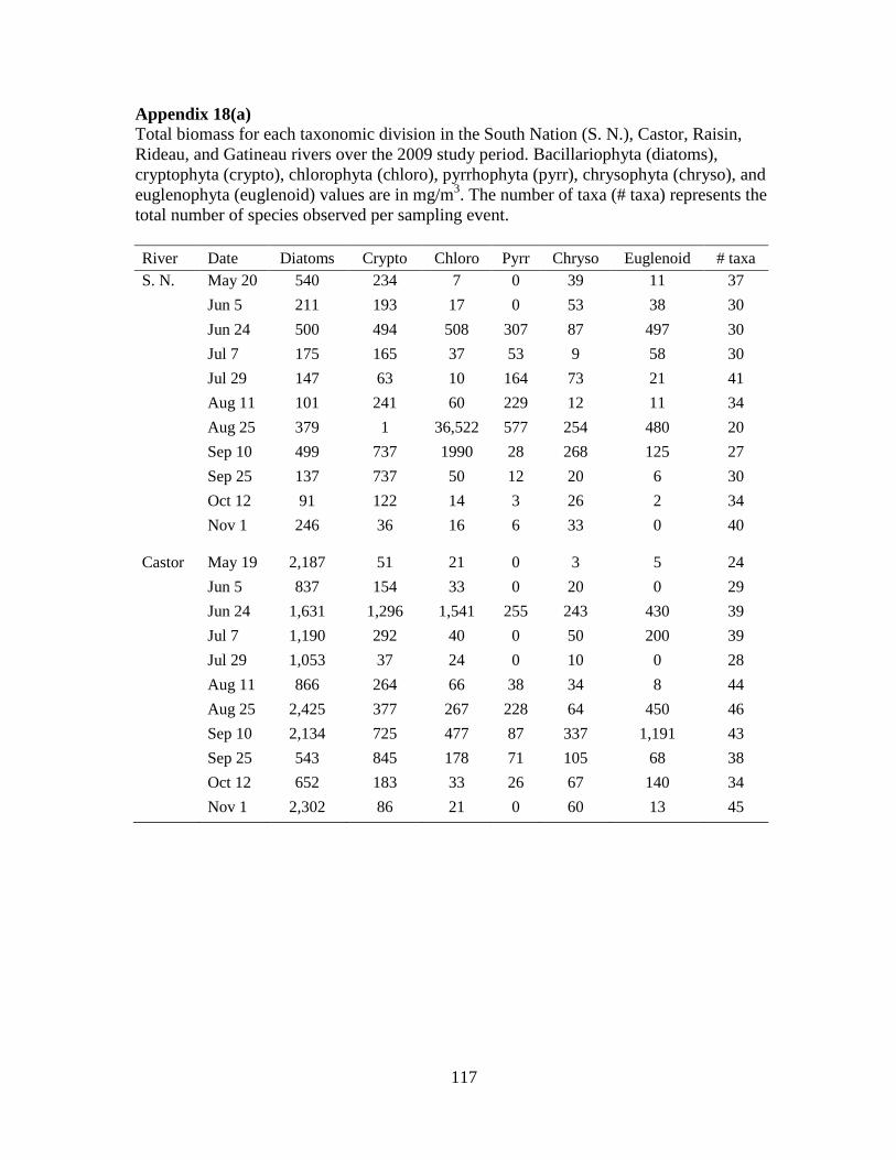
117
Appendix 18(a)
Total biomass for each taxonomic division in the South Nation (S. N.), Castor, Raisin,
Rideau, and Gatineau rivers over the 2009 study period. Bacillariophyta (diatoms),
cryptophyta (crypto), chlorophyta (chloro), pyrrhophyta (pyrr), chrysophyta (chryso), and
euglenophyta (euglenoid) values are in mg/m3. The number of taxa (# taxa) represents the
total number of species observed per sampling event.
River Date Diatoms Crypto Chloro Pyrr Chryso Euglenoid # taxa
S. N. May 20 540 234 7 0 39 11 37
Jun 5 211 193 17 0 53 38 30
Jun 24 500 494 508 307 87 497 30
Jul 7 175 165 37 53 9 58 30
Jul 29 147 63 10 164 73 21 41
Aug 11 101 241 60 229 12 11 34
Aug 25 379 1 36,522 577 254 480 20
Sep 10 499 737 1990 28 268 125 27
Sep 25 137 737 50 12 20 6 30
Oct 12 91 122 14 3 26 2 34
Nov 1 246 36 16 6 33 0 40
Castor May 19 2,187 51 21 0 3 5 24
Jun 5 837 154 33 0 20 0 29
Jun 24 1,631 1,296 1,541 255 243 430 39
Jul 7 1,190 292 40 0 50 200 39
Jul 29 1,053 37 24 0 10 0 28
Aug 11 866 264 66 38 34 8 44
Aug 25 2,425 377 267 228 64 450 46
Sep 10 2,134 725 477 87 337 1,191 43
Sep 25 543 845 178 71 105 68 38
Oct 12 652 183 33 26 67 140 34
Nov 1 2,302 86 21 0 60 13 45
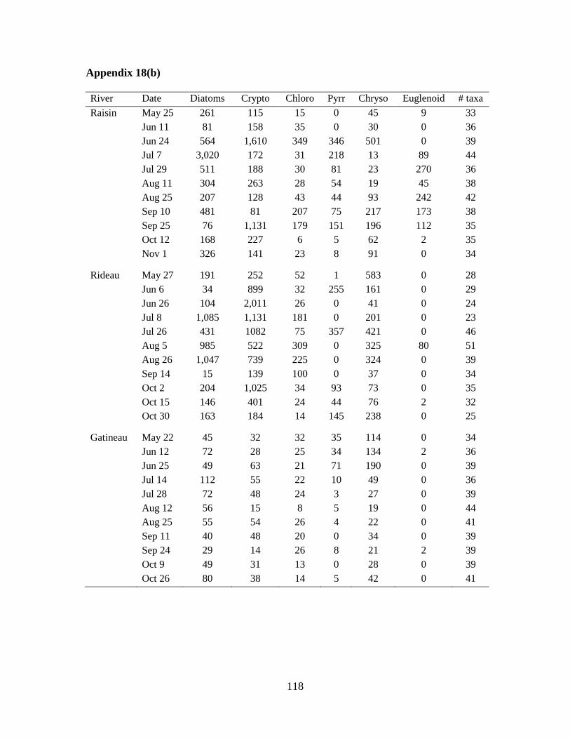
118
Appendix 18(b)
River Date Diatoms Crypto Chloro Pyrr Chryso Euglenoid # taxa
Raisin May 25 261 115 15 0 45 9 33
Jun 11 81 158 35 0 30 0 36
Jun 24 564 1,610 349 346 501 0 39
Jul 7 3,020 172 31 218 13 89 44
Jul 29 511 188 30 81 23 270 36
Aug 11 304 263 28 54 19 45 38
Aug 25 207 128 43 44 93 242 42
Sep 10 481 81 207 75 217 173 38
Sep 25 76 1,131 179 151 196 112 35
Oct 12 168 227 6 5 62 2 35
Nov 1 326 141 23 8 91 0 34
Rideau May 27 191 252 52 1 583 0 28
Jun 6 34 899 32 255 161 0 29
Jun 26 104 2,011 26 0 41 0 24
Jul 8 1,085 1,131 181 0 201 0 23
Jul 26 431 1082 75 357 421 0 46
Aug 5 985 522 309 0 325 80 51
Aug 26 1,047 739 225 0 324 0 39
Sep 14 15 139 100 0 37 0 34
Oct 2 204 1,025 34 93 73 0 35
Oct 15 146 401 24 44 76 2 32
Oct 30 163 184 14 145 238 0 25
Gatineau May 22 45 32 32 35 114 0 34
Jun 12 72 28 25 34 134 2 36
Jun 25 49 63 21 71 190 0 39
Jul 14 112 55 22 10 49 0 36
Jul 28 72 48 24 3 27 0 39
Aug 12 56 15 8 5 19 0 44
Aug 25 55 54 26 4 22 0 41
Sep 11 40 48 20 0 34 0 39
Sep 24 29 14 26 8 21 2 39
Oct 9 49 31 13 0 28 0 39
Oct 26 80 38 14 5 42 0 41