Pidar: 3D Laser Range Finder

Pidar: 3D Laser Range Finder

Group 27

Jonathan Ulrich Andrew Watson

Sponsored By: Robotics Club at the University of Central

Florida

i

Table of Contents 1. Introduction .................................................................................................................1

1.1. Executive Summary .......................................................................................... 1

1.2. Project Motivation and Goals ........................................................................... 2

2. Objectives, Specifications, and Budget ..................................................................3

2.1. Project Requirements and Specifications ...................................................... 4

2.2. Budget ................................................................................................................. 4

2.3. Timeline ............................................................................................................... 5

2.3.1. January ........................................................................................................ 5

2.3.2. February....................................................................................................... 5

2.3.3. March ........................................................................................................... 5

2.3.4. April............................................................................................................... 6

3. Research .....................................................................................................................7

3.1. Similar Proposals and Projects ....................................................................... 7

3.1.1. 3DLS-Ks Continuous Rotation ................................................................. 8

3.1.2. Dynamixel Hokuyo Coupling .................................................................... 9

3.1.3. UnoLaser 30M135Y ................................................................................... 9

3.2. Laser Sensors (LIDAR)................................................................................... 10

3.2.1. Hokuyo PBS .............................................................................................. 10

3.2.2. Hokuyo URG-04LX-UG01 ...................................................................... 11

3.2.3. Hokuyo UBG-04LX-F01 .......................................................................... 12

3.2.4. Hokuyo URG-04LX .................................................................................. 13

3.2.5. Hokuyo UTM-30LX................................................................................... 13

3.2.6. Comparison of Lasers ............................................................................. 14

3.3. 3D Scanning Implementations ...................................................................... 15

3.3.1. Rolling Scan .............................................................................................. 15

3.3.2. Pitching Scan ............................................................................................ 16

3.3.3. Yawing Scan ............................................................................................. 17

3.3.4. Comparison of Scanning Implementations .......................................... 18

3.3.5. Open Loop Control ................................................................................... 19

3.3.6. Closed Loop Control ................................................................................ 20

3.4. Motor Control .................................................................................................... 22

ii

3.4.1. Micro stepping........................................................................................... 22

3.4.2. SM-42BYG011-25 Stepper Motor ......................................................... 23

3.4.3. 42BYGHM809 Stepper Motor ................................................................ 23

3.4.4. A3967 Micro stepping Driver .................................................................. 24

3.4.5. STMicro's L6470 Stepper Motor Driver ................................................ 24

3.4.6. Servo .......................................................................................................... 24

3.4.7. Hitec HS-805BB Servo Motor................................................................. 25

3.4.8. Dynamixel MX-28T Robot Actuator ....................................................... 25

3.4.9. DC Motor Control ..................................................................................... 26

3.4.10. KM-12FN20-100-06120 DC Motor ..................................................... 26

3.4.11. GB37Y3530-12V-83R DC Motor ........................................................ 26

3.4.12. Encoders ................................................................................................ 27

3.4.13. E6A2-CS3E Rotary Encoder .............................................................. 27

3.4.14. A6B2-CWZ3E-1024 Rotary Encoder ................................................. 27

3.4.15. Comparison of Motors ......................................................................... 28

3.5. Microcontrollers / Computing ......................................................................... 29

3.5.1. Raspberry Pi ............................................................................................. 30

3.5.2. Beagle Board Black ................................................................................. 30

3.5.3. Panda Board ES ....................................................................................... 30

3.5.4. Comparison of Microcontrollers ............................................................. 31

3.6. Power................................................................................................................. 33

3.6.1. Regulation ................................................................................................. 34

3.6.2. TI LMZ14203 Simple Switcher ............................................................... 34

3.6.3. TI LM7805CV Linear Voltage Regulator .............................................. 35

3.6.4. CUIINC V78-2000 .................................................................................... 36

3.7. Waterproof Connectors .................................................................................. 37

3.7.1. Weipu Connectors .................................................................................... 37

3.7.2. Bulgin Buccaneer Connectors ................................................................ 38

3.8. Data Representation Software ...................................................................... 40

3.8.1. Depth Imaging........................................................................................... 41

3.8.2. OpenCV ..................................................................................................... 42

3.8.3. SimpleCV ................................................................................................... 42

3.8.4. PDAL .......................................................................................................... 43

4. Design ........................................................................................................................44

iii

4.1. Hardware Design ............................................................................................. 44

4.1.1. Hokuyo UTM-30LX 2D Laser Range Finder ........................................ 45

4.1.2. Timing......................................................................................................... 46

4.1.3. Power Requirements ............................................................................... 47

4.1.4. Raspberry Pi Model B .............................................................................. 48

4.1.5. Dynamixel MX-28T Robot Actuator ....................................................... 50

4.1.6. Motion......................................................................................................... 52

4.2. Software Design .............................................................................................. 53

4.2.1. Laser Communication .............................................................................. 54

4.2.2. Dynamixel MX-28T Servo Communication .......................................... 56

4.2.3. Webcam Communication ........................................................................ 56

4.2.4. Platform Communication ......................................................................... 57

4.2.5. 3D Creation ............................................................................................... 58

4.2.6. Point Cloud ................................................................................................ 59

4.2.7. Real World Image..................................................................................... 61

4.2.8. Dynamic Configuration ............................................................................ 62

4.2.9. User Interfaces ......................................................................................... 63

4.2.10. Network Access .................................................................................... 64

4.2.11. Output Protocol ..................................................................................... 65

4.2.12. Command Sequence ........................................................................... 69

4.2.13. Output ..................................................................................................... 71

4.2.14. Linux ....................................................................................................... 72

4.2.15. Raspien OpenCV Package ................................................................. 73

4.2.16. Programming Languages .................................................................... 73

4.2.17. IDE .......................................................................................................... 74

5. Executive Design Summary ...................................................................................75

5.1. 2D Laser Specifications .................................................................................. 75

5.2. Software Structures ......................................................................................... 76

5.3. Parts................................................................................................................... 78

5.4. Program Functions .......................................................................................... 78

6. Construction, Testing, and Evaluation ..................................................................80

6.1. 2D Laser ............................................................................................................ 80

6.2. Motor .................................................................................................................. 81

6.3. Microcontroller .................................................................................................. 82

iv

6.3.1. Power and Regulation ............................................................................. 82

6.3.2. Input and Output ....................................................................................... 82

6.4. Software Unit Testing ...................................................................................... 83

6.5. System Performance ...................................................................................... 84

6.5.1. Regular Environment ............................................................................... 84

6.5.2. Outside Environment ............................................................................... 89

6.5.3. Project Summary ...................................................................................... 90

7. Bibliography ..............................................................................................................91

A. Copyright Permissions ............................................................................................93

Table of Figures Figure 1 Kinect Depth Image .......................................................................................... 2

Figure 2 3DLS Continuous Rotation 3D-Laser-Scanner ............................................ 8

Figure 3 3D Rotating Design .......................................................................................... 9

Figure 4 Uno Engineering UnoLaser 30M135Y 3D LIDAR ..................................... 10

Figure 5 Hokuyo PBS .................................................................................................... 11

Figure 6 Hokuyo URG-04LX-UG01 ............................................................................. 12

Figure 7 Hokuyo UBG-04LX-F01 ................................................................................ 12

Figure 8 Hokuyo URG-04LX ........................................................................................ 13

Figure 9 Hokuyo UTM-30LX ......................................................................................... 14

Figure 10 Rolling Scan Coverage ................................................................................ 16

Figure 11 Pitching Scan Coverage .............................................................................. 17

Figure 12 Yawing Scan Coverage (Side Mount) ....................................................... 18

Figure 13 Basic Open Loop Control Path .................................................................. 20

Figure 14 Basic Closed Loop Control Path ................................................................ 22

Figure 15 SM-42BYG011-25 Stepper Motor ............................................................. 23

Figure 16 Hitec HS-805BB Servo Motor..................................................................... 25

Figure 17 M-12FN20-100-06120 DC Motor ............................................................... 26

Figure 18 E6A2-CS3E Rotary Encoder ...................................................................... 27

Figure 19 Example Circuit Using LMZ14203 Switching Regulator ........................ 35

Figure 20 Example Circuit Using the TI LM7805CV ................................................. 36

Figure 21 Weipu Connectors Mounted ....................................................................... 38

Figure 22 Point Cloud Image ........................................................................................ 40

Figure 23 Hardware Block Diagram ............................................................................ 44

Figure 24 Hokuyo UTM-30LX Scan Steps ................................................................. 45

Figure 25 LIDAR Sync Pulse ........................................................................................ 46

Figure 26 Pinout of the TXB0108 8-Channel Logic Level Converter ..................... 48

Figure 27 Laser Mount Outline .................................................................................... 51

Figure 28 Pitching Scan Prototype .............................................................................. 52

Figure 29 Rolling Scan Model ...................................................................................... 53

v

Figure 30 Software Block Diagram .............................................................................. 54

Figure 31 Oscilloscope Output of Laser Synchronization Signal ........................... 55

Figure 32 Projecting 2D Image from Radial Scan .................................................... 59

Figure 33 Point Cloud Representation ........................................................................ 60

Figure 34 Range Image ................................................................................................ 61

Figure 35 Graphical User Interface Mockup .............................................................. 63

Figure 36 Hokuyo 2D Dimensions ............................................................................... 75

Figure 37 Sequence Diagram for Normal Operations .............................................. 77

Figure 38 Sequence Diagram for Setting Changes .................................................. 77

Figure 39 Image Class Diagram .................................................................................. 79

Figure 40 Communications Class Diagram ............................................................... 80

Figure 41 Camera Image of Clear Hallway ................................................................ 85

Figure 42 Point Cloud of Clear Hallway ...................................................................... 86

Figure 43 Depth Colored Point Cloud ......................................................................... 87

Figure 44 Range Image Comparison With Camera Image ..................................... 88

Figure 45 Nighttime Scan Outside .............................................................................. 89

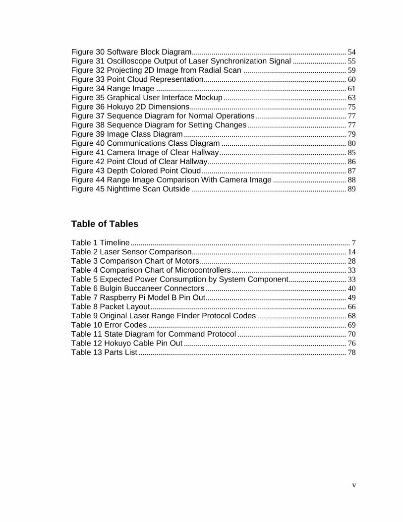
Table of Tables Table 1 Timeline ............................................................................................................... 7

Table 2 Laser Sensor Comparison .............................................................................. 14

Table 3 Comparison Chart of Motors .......................................................................... 28

Table 4 Comparison Chart of Microcontrollers .......................................................... 33

Table 5 Expected Power Consumption by System Component ............................. 33

Table 6 Bulgin Buccaneer Connectors ....................................................................... 40

Table 7 Raspberry Pi Model B Pin Out ....................................................................... 49

Table 8 Packet Layout ................................................................................................... 66

Table 9 Original Laser Range FInder Protocol Codes ............................................. 68

Table 10 Error Codes .................................................................................................... 69

Table 11 State Diagram for Command Protocol ....................................................... 70

Table 12 Hokuyo Cable Pin Out .................................................................................. 76

Table 13 Parts List ......................................................................................................... 78

1

1. Introduction

1.1. Executive Summary Since its inception in 2002 the Robotics Club at UCF has pushed students and volunteers to the cutting edge of technology and innovation. Through annual participation in multiple international autonomous robotics competitions and outreach programs the club has excelled in generating robotic platforms capable of increasingly complex tasks. These competitions, primarily hosted by the Association for Unmanned Vehicle Systems International (AUVSI), include a variety of different kinds of platforms such as surface, ground, and underwater based vehicles. While upon initial inspection it may seem that such platforms operating in completely different environments would be vastly different, they are instead very similar in accomplishing some of the basic tasks required for autonomy. Since all of the platforms require interaction with their environment being able to sense their surroundings accurately has proven difficult for the organization to manage across multiple platforms without extreme cost. Of the many sensors outfitted on the varying vehicles there is one which universally provides an ample amount of real time data for the necessary autonomy. Light Detection and Ranging (LIDAR) scanners are used on the largest of the platforms fabricated in the club and are great for obstacle detection and avoidance. While previous attempts at using the raw 2D data from these sensors for map generation has proven beneficial observing a 3D world from 2D data is never an ideal scenario. It is the goal of this design group of computer engineers to enable 3 dimensional sensing from the physical rotation of a 2D laser scanner for use on these platforms. Power input into the rotating system will be different based on the available power regulation requirements of the robotic platforms themselves. It is expected that power into this system will potentially be cut off at any time from emergency stop systems and therefore must be capable of compensating for power spikes and total power loss. Such a system must also be able to accept a range of input voltage levels and be able to compensate for inconsistencies via loss throughout the system. With the intended end application of the sensor being an outdoor environment protection of sensitive electronics and waterproofing of cables routed to and from the vehicle and system is of utmost importance. Management of cables is also crucial to the system as the sensor is being physically moved or rotated increasing the probability of kinks or snags with either the vehicle or the system itself. Different approaches can be taken to minimize this risk by implementing different rotation schemes or to avoid it by going completely wireless. Fabrication of an embedded system for use in different robots assumes a variety of available mounting solutions be made available. Dependent on the rotation

2

scheme chosen mounting of the sensor about the appropriate rotation axis should improve accuracy of 3D measurements. Offloading sensor reading to an external system enables more computational resources for the platform itself for other demanding tasks such as computer vision. Simplified connectors and software interfaces provide seamless integration with existing systems. Communication between the robots and embedded laser system is therefore crucial in guaranteeing interoperability. Abstracting a generalized interface for commanding, packaging, and receiving scan data must be as much of a priority as is the data itself. Leveraging the Joint Architecture for Unmanned Systems (JAUS) architecture as a starting point will ensure that the existing capabilities of the robots will mesh properly with the proposed laser scanner.

1.2. Project Motivation and Goals With the increasing complexity of modern manufacturing and the birth of 3D printing the demand for acquiring spatial data from an environment has never been higher. Whether it is a desktop 3D printer or an autonomous car there have been many breakthroughs in the past few years which have expanded the ability of current light based detection and ranging sensors. These advancements come at a price and that price is often in the tens of thousands of dollars. Lower cost alternatives have been on the market for some time and have come in some surprising forms but usually have tradeoffs. The Xbox Kinect for example is a gaming camera device that can achieve many of these functions but fails to work outside or at long distances due to its IR camera. Figure 1 demonstrates the sensors capabilities indoors.

(Reprinted with permission through fair use policy)

Figure 1 Kinect Depth Image

The goal of this project was to create a three-dimensional sensor capable of remaining low cost while still retaining all of the accuracy, precision, and speed of higher cost solutions. While the final assembly has many useful functions, the primary role is the utilization by the Robotics Club at UCF for their many autonomous robotic platforms. Robotic platforms have a uniquely high

3

dependency on the speed and accuracies of such sensors in order to interact within dynamic environments reliably. Over the many years of intense competition with a variety of platforms across multiple teams the Robotics Club at UCF has consistently found a need for collecting highly accurate 3D data from the environment. The tasks expected of the autonomous vehicles built are outlined in the various collegiate level robotics competitions sponsored by AUVSI including mainly the IGVC, Roboboat, and Robosub competitions. While initially these competitions may appear to be as different as the diverse platforms designed for them, in fact, they share almost all of the same underlying proficiencies. The vehicles competing in these competitions must all be able to interact with and react to changes in their environment in a real-time application. Building a system with such a capability normally requires construction of a modest map which innately relies on the precision of the sensors used in its generation. Approaches by previous robotics teams generally attempt to leverage simple 2D data for primitive obstacle avoidance techniques which have proven mildly effective. To completely and reliably map a real-world environment however one must consider all dimensions at once to fully construct a true representation. Attempts have been made by the organization to construct such data, but fragmentation in development and the loss of computational power by such systems has deterred further development. The club has identified this need in recent years and have tasked this group with coming up with a solution to this problem. The club has generously offered to donate a fast, long range 2D laser range finder to help in the construction of the proposed system.

2. Objectives, Specifications, and Budget Functionally speaking the project is a fully embedded 3D solution leveraging a very capable 2D laser scanner. In order to generate 3D data the sensor is placed upon a fabricated mount which physically moves the sensor about an axis of rotation. The mechanical device does not restrict the wide field of view of the sensor itself and in addition should minimize translational errors due to physical sensor movement during scans. Many software features were planned including accurate depth mapping and live perspective transforming to real time camera feeds. This data is sent out via a network connection in the system. This standard allows for streaming of image data generated from each full scan real-time to multiple platforms if desired across a network. It also enables an ‘always on’ operation of the sensor further emphasizing the systems embedded nature.

4

2.1. Project Requirements and Specifications The Robotics Club at UCF generated a formal list of requirements that the project should have adhered to. These technical requirements given by the organization and other more generic specifications are listed below by category:

Physical Occupy less than 3 cubic feet. Mounting options on 2 axes. Weigh less than 5 pounds.

Scans

Scanning time will be 1.5 sec / scan or better for 45° scans. The assembly will be capable of at least 160° horizontal F.O.V. The assembly will be capable of at least 90° vertical F.O.V. Angular resolution on all axes will be at least 0.5° or better. Ranges from 0.1 to 30 meters. Real time configuration of these parameters.

Power

Will run on a single power rail (12/24 V). Maximum power consumption will not exceed 36 W. Onboard regulation for all components. Onboard voltage monitoring

Interfaces

PC connection (Ethernet / USB) Power connection Connectors must be waterproof

Software

SAE JAUS compliance. ‘Always On’ operation of the system. Drivers, visualization, and monitoring software will be cross-platform. All software will be open-sourced and well documented.

Operating Conditions

Performance will be identical both in indoor / outdoor environments. Operating temperatures will be from at least 0 to +50° C. System must be weatherproof, IP Standard 45 or better.

2.2. Budget This project is funded generously by the Robotics Club at UCF from their in-house funds and through the various sponsors of the organization. The 2D laser provided is the most expensive component of the project and was being loaned

5

for the groups use. The group estimates total cost of the project to be around $7,000 .00 total. Table 1 outlines the projected costs of various components of the project and exactly what has and has not been acquired.

2.3. Timeline

2.3.1. January We began the creation of the 3D laser range finder by preparing our environment. We built and installed the operating system for the raspberry Pi. Once we have installed the operating system began creating our basic hardware access functions. We created small callable functions that each can access the GPIO pins and provide methods to listen or provide output. We installed and configured the library for the Hokuyo laser scanner and created functions that are able to access and utilize it. The rotation of the laser scanner was the next part we will needed to create. This included 3D modeling of the part, printing the part on a 3D printer and mounting it to our motor. This provided us with a prototype while we create the software.

2.3.2. February We created the necessary functions that will utilize the Point Cloud Library. This required us to modify the code in order to run it on our processor. Then we built the libraries and installed them into our system. Once we had the libraries installed, we will need to create our more advanced methods that combine some of our functions. At this point we hoped to be able to take test data and pass it through our system and provide some sort of resemblance to our output data. However, we were unable to do so at this point. Once the basic functions have been created, we began the creation of the output API. This will require the creation of many functions for communication. We hoped to create listeners that will wait for requests, create input and output buffers, and create encoding and decoding classes that will be used. The different actions will basically be “scripted” mechanisms that will respond to the different action codes. This should have all adhered to our new communication protocol. The parts we ordered had come in at this point and we built prototype circuits for testing. We tested our system so that each of the components will function correctly.

2.3.3. March We now focused on the software generation and output. The software that we needed to create will combine all of the different functions and act as our central control system. We hoped be able to have all the software completed by this

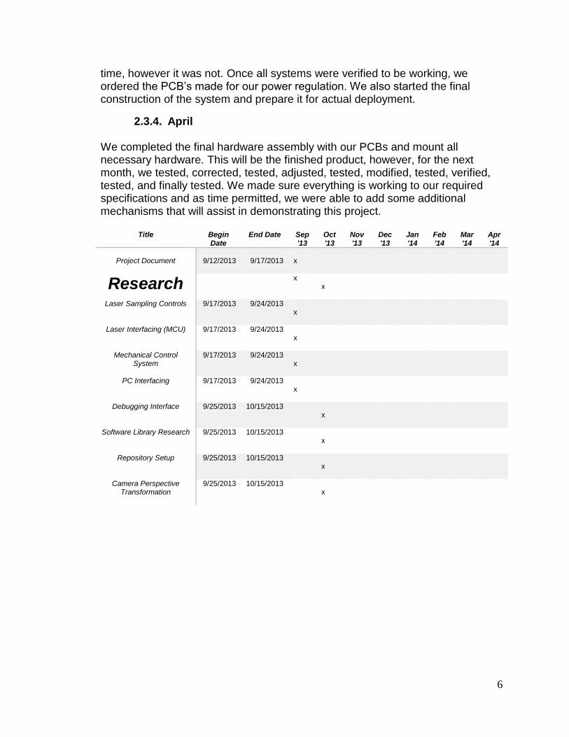
6

time, however it was not. Once all systems were verified to be working, we ordered the PCB’s made for our power regulation. We also started the final construction of the system and prepare it for actual deployment.

2.3.4. April We completed the final hardware assembly with our PCBs and mount all necessary hardware. This will be the finished product, however, for the next month, we tested, corrected, tested, adjusted, tested, modified, tested, verified, tested, and finally tested. We made sure everything is working to our required specifications and as time permitted, we were able to add some additional mechanisms that will assist in demonstrating this project.

Title Begin Date

End Date Sep '13

Oct '13

Nov '13

Dec '13

Jan '14

Feb '14

Mar '14

Apr '14

Project Document

9/12/2013

9/17/2013

x

Research

x

x

Laser Sampling Controls 9/17/2013 9/24/2013 x

Laser Interfacing (MCU) 9/17/2013 9/24/2013 x

Mechanical Control System

9/17/2013 9/24/2013 x

PC Interfacing 9/17/2013 9/24/2013 x

Debugging Interface 9/25/2013 10/15/2013

x

Software Library Research 9/25/2013 10/15/2013

x

Repository Setup 9/25/2013 10/15/2013

x

Camera Perspective Transformation

9/25/2013 10/15/2013

x

7

Begin Date End Date Sep

'13 Oct '13

Nov '13

Dec '13

Jan '14

Feb '14

Mar '14

Apr '14

Design

10/16/2013

12/31/2013

Tilting Mount 10/16/2013

10/31/2013

X

PCB Design 12/1/2013

12/31/2013

X

Driver Software 10/16/2013

12/31/2013

X

X

X

PC Software 10/16/2013

11/30/2013

X

X

Electrical Components 10/16/2013

12/31/2013

X

X

X

Build 12/15/2013 4/30/2014

PCB Board

2/1/2014

3/31/2014

X

X

PC Driver Board 12/15/2013

1/15/2014

X

X

PC Software 1/1/2014

2/28/2014

X

X

Laser Scanner 12/15/2013

1/31/2014

X

X

Testing

Continuously

12/15/2014

4/30/2014

X

X

X

X

X

Table 1 Timeline

3. Research

3.1. Similar Proposals and Projects There have been many attempts at utilizing the Hokuyo UTM-30LX LIDAR as a low cost full 3D laser scanner. This section will highlight systems implementing 3D laser designs and present different methods of adding an extra dimension to the normal 2D data. Many of the technologies presented are available as commercial products wherein teams of professional engineers have carefully and meticulously sought after efficient solutions. It was the goal of this project to

8

accumulate the best approaches, techniques, and ideas of those available in order to provide the best solution in the end design.

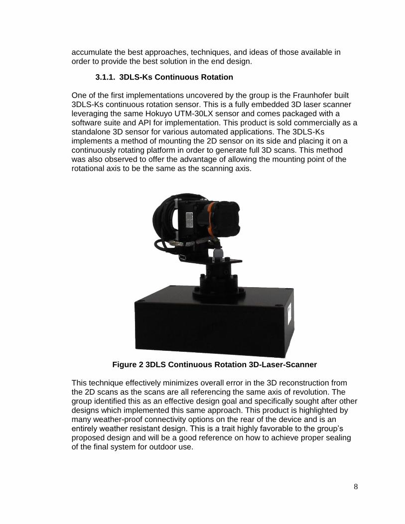
3.1.1. 3DLS-Ks Continuous Rotation One of the first implementations uncovered by the group is the Fraunhofer built 3DLS-Ks continuous rotation sensor. This is a fully embedded 3D laser scanner leveraging the same Hokuyo UTM-30LX sensor and comes packaged with a software suite and API for implementation. This product is sold commercially as a standalone 3D sensor for various automated applications. The 3DLS-Ks implements a method of mounting the 2D sensor on its side and placing it on a continuously rotating platform in order to generate full 3D scans. This method was also observed to offer the advantage of allowing the mounting point of the rotational axis to be the same as the scanning axis.

Figure 2 3DLS Continuous Rotation 3D-Laser-Scanner

This technique effectively minimizes overall error in the 3D reconstruction from the 2D scans as the scans are all referencing the same axis of revolution. The group identified this as an effective design goal and specifically sought after other designs which implemented this same approach. This product is highlighted by many weather-proof connectivity options on the rear of the device and is an entirely weather resistant design. This is a trait highly favorable to the group’s proposed design and will be a good reference on how to achieve proper sealing of the final system for outdoor use.

9

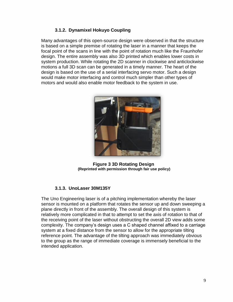
3.1.2. Dynamixel Hokuyo Coupling Many advantages of this open-source design were observed in that the structure is based on a simple premise of rotating the laser in a manner that keeps the focal point of the scans in line with the point of rotation much like the Fraunhofer design. The entire assembly was also 3D printed which enables lower costs in system production. While rotating the 2D scanner in clockwise and anticlockwise motions a full 3D scan can be generated in a timely manner. The heart of the design is based on the use of a serial interfacing servo motor. Such a design would make motor interfacing and control much simpler than other types of motors and would also enable motor feedback to the system in use.

Figure 3 3D Rotating Design


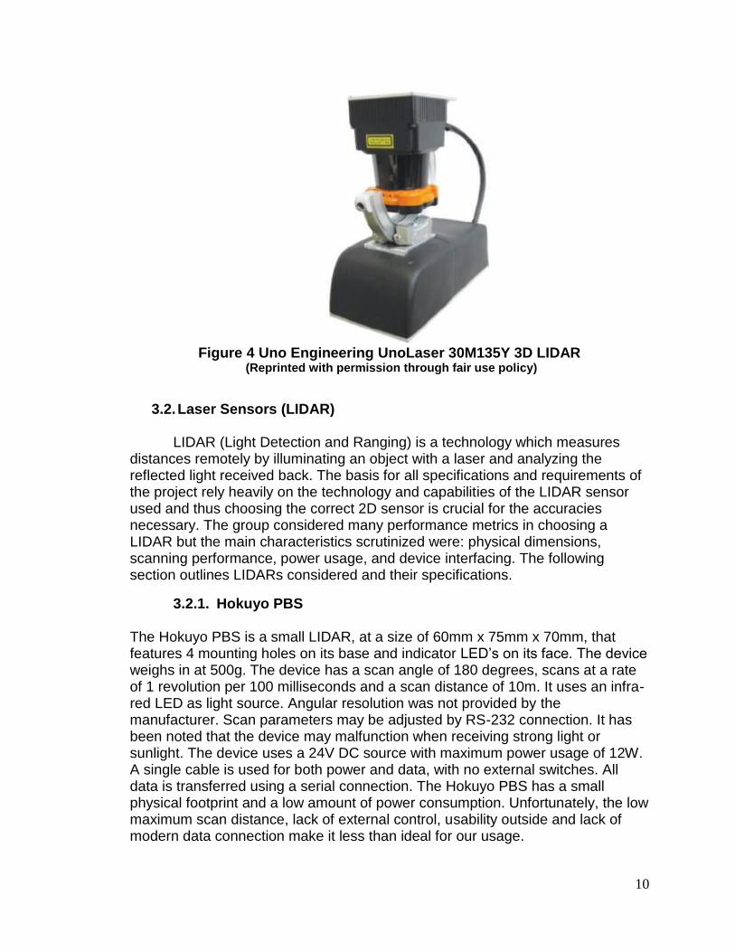
3.1.3. UnoLaser 30M135Y The Uno Engineering laser is of a pitching implementation whereby the laser sensor is mounted on a platform that rotates the sensor up and down sweeping a plane directly in front of the assembly. The overall design of this system is relatively more complicated in that to attempt to set the axis of rotation to that of the receiving point of the laser without obstructing the overall 2D view adds some complexity. The company’s design uses a C shaped channel affixed to a carriage system at a fixed distance from the sensor to allow for the appropriate tilting reference point. The advantage of the tilting approach was immediately obvious to the group as the range of immediate coverage is immensely beneficial to the intended application.

10

Figure 4 Uno Engineering UnoLaser 30M135Y 3D LIDAR


3.2. Laser Sensors (LIDAR)

LIDAR (Light Detection and Ranging) is a technology which measures distances remotely by illuminating an object with a laser and analyzing the reflected light received back. The basis for all specifications and requirements of the project rely heavily on the technology and capabilities of the LIDAR sensor used and thus choosing the correct 2D sensor is crucial for the accuracies necessary. The group considered many performance metrics in choosing a LIDAR but the main characteristics scrutinized were: physical dimensions, scanning performance, power usage, and device interfacing. The following section outlines LIDARs considered and their specifications.

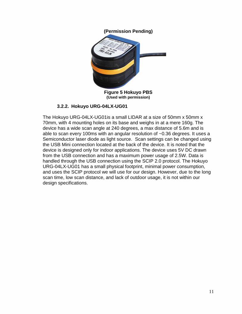
3.2.1. Hokuyo PBS The Hokuyo PBS is a small LIDAR, at a size of 60mm x 75mm x 70mm, that features 4 mounting holes on its base and indicator LED’s on its face. The device weighs in at 500g. The device has a scan angle of 180 degrees, scans at a rate of 1 revolution per 100 milliseconds and a scan distance of 10m. It uses an infra-red LED as light source. Angular resolution was not provided by the manufacturer. Scan parameters may be adjusted by RS-232 connection. It has been noted that the device may malfunction when receiving strong light or sunlight. The device uses a 24V DC source with maximum power usage of 12W. A single cable is used for both power and data, with no external switches. All data is transferred using a serial connection. The Hokuyo PBS has a small physical footprint and a low amount of power consumption. Unfortunately, the low maximum scan distance, lack of external control, usability outside and lack of modern data connection make it less than ideal for our usage.

11

(Permission Pending)

Figure 5 Hokuyo PBS

(Used with permission)

3.2.2. Hokuyo URG-04LX-UG01 The Hokuyo URG-04LX-UG01is a small LIDAR at a size of 50mm x 50mm x 70mm, with 4 mounting holes on its base and weighs in at a mere 160g. The device has a wide scan angle at 240 degrees, a max distance of 5.6m and is able to scan every 100ms with an angular resolution of ~0.36 degrees. It uses a Semiconductor laser diode as light source. Scan settings can be changed using the USB Mini connection located at the back of the device. It is noted that the device is designed only for indoor applications. The device uses 5V DC drawn from the USB connection and has a maximum power usage of 2.5W. Data is handled through the USB connection using the SCIP 2.0 protocol. The Hokuyo URG-04LX-UG01 has a small physical footprint, minimal power consumption, and uses the SCIP protocol we will use for our design. However, due to the long scan time, low scan distance, and lack of outdoor usage, it is not within our design specifications.

12

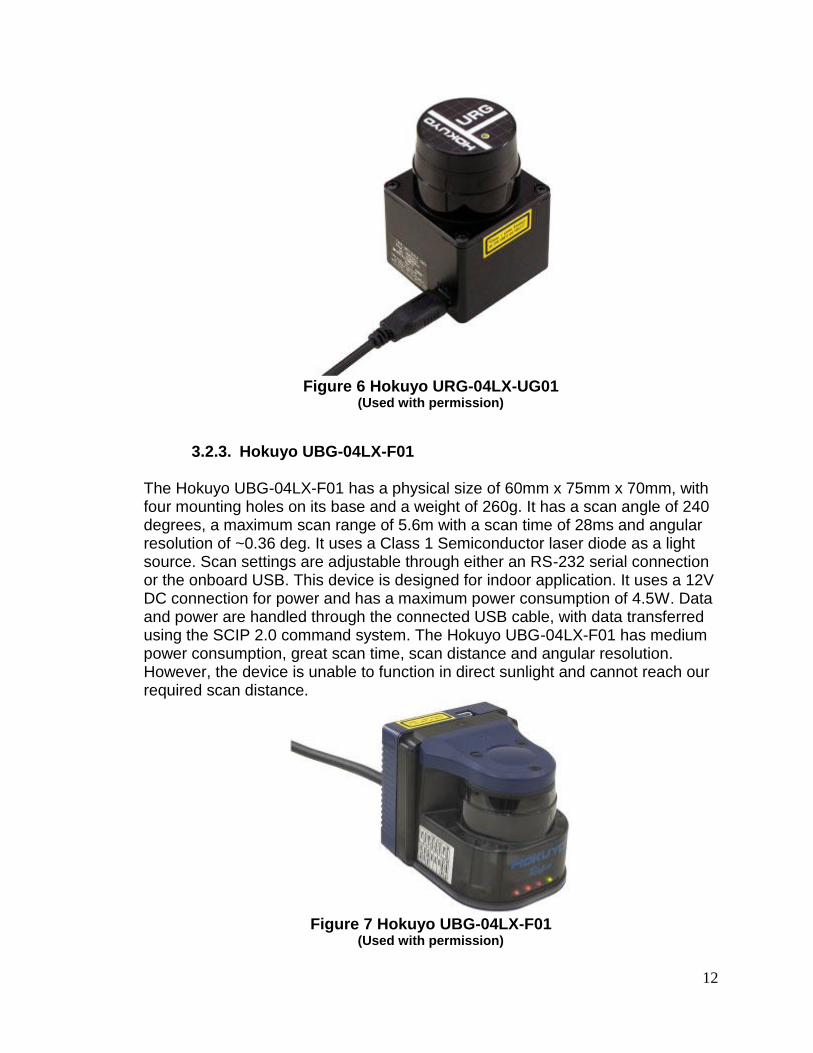
Figure 6 Hokuyo URG-04LX-UG01


3.2.3. Hokuyo UBG-04LX-F01 The Hokuyo UBG-04LX-F01 has a physical size of 60mm x 75mm x 70mm, with four mounting holes on its base and a weight of 260g. It has a scan angle of 240 degrees, a maximum scan range of 5.6m with a scan time of 28ms and angular resolution of ~0.36 deg. It uses a Class 1 Semiconductor laser diode as a light source. Scan settings are adjustable through either an RS-232 serial connection or the onboard USB. This device is designed for indoor application. It uses a 12V DC connection for power and has a maximum power consumption of 4.5W. Data and power are handled through the connected USB cable, with data transferred using the SCIP 2.0 command system. The Hokuyo UBG-04LX-F01 has medium power consumption, great scan time, scan distance and angular resolution. However, the device is unable to function in direct sunlight and cannot reach our required scan distance.

Figure 7 Hokuyo UBG-04LX-F01


13

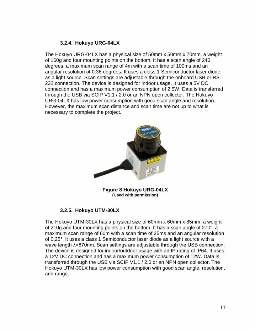
3.2.4. Hokuyo URG-04LX The Hokuyo URG-04LX has a physical size of 50mm x 50mm x 70mm, a weight of 160g and four mounting points on the bottom. It has a scan angle of 240 degrees, a maximum scan range of 4m with a scan time of 100ms and an angular resolution of 0.36 degrees. It uses a class 1 Semiconductor laser diode as a light source. Scan settings are adjustable through the onboard USB or RS-232 connection. The device is designed for indoor usage. It uses a 5V DC connection and has a maximum power consumption of 2.5W. Data is transferred through the USB via SCIP V1.1 / 2.0 or an NPN open collector. The Hokuyo URG-04LX has low power consumption with good scan angle and resolution. However, the maximum scan distance and scan time are not up to what is necessary to complete the project.

Figure 8 Hokuyo URG-04LX


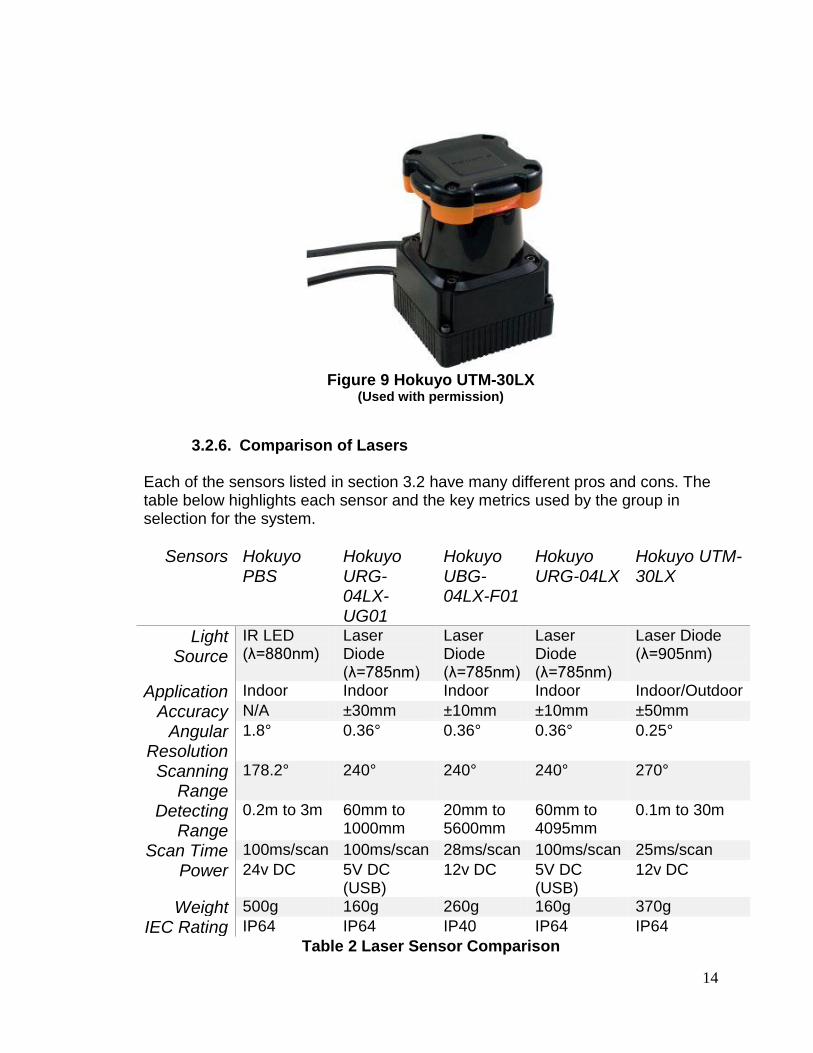
3.2.5. Hokuyo UTM-30LX The Hokuyo UTM-30LX has a physical size of 60mm x 60mm x 85mm, a weight of 210g and four mounting points on the bottom. It has a scan angle of 270°, a maximum scan range of 60m with a scan time of 25ms and an angular resolution of 0.25°. It uses a class 1 Semiconductor laser diode as a light source with a wave length λ=870nm. Scan settings are adjustable through the USB connection. The device is designed for indoor/outdoor usage with an IP rating of IP64. It uses a 12V DC connection and has a maximum power consumption of 12W. Data is transferred through the USB via SCIP V1.1 / 2.0 or an NPN open collector. The Hokuyo UTM-30LX has low power consumption with good scan angle, resolution, and range.

14

Figure 9 Hokuyo UTM-30LX


3.2.6. Comparison of Lasers Each of the sensors listed in section 3.2 have many different pros and cons. The table below highlights each sensor and the key metrics used by the group in selection for the system.

Sensors Hokuyo PBS

Hokuyo URG-04LX-UG01

Hokuyo UBG-04LX-F01

Hokuyo URG-04LX

Hokuyo UTM-30LX

Light Source

IR LED (λ=880nm)

Laser Diode (λ=785nm)




Application Indoor Indoor Indoor Indoor Indoor/Outdoor

Accuracy N/A ±30mm ±10mm ±10mm ±50mm

Angular Resolution

1.8° 0.36° 0.36° 0.36° 0.25°

Scanning Range

178.2° 240° 240° 240° 270°

Detecting Range

0.2m to 3m 60mm to 1000mm

20mm to 5600mm

60mm to 4095mm

0.1m to 30m

Scan Time 100ms/scan 100ms/scan 28ms/scan 100ms/scan 25ms/scan

Power 24v DC 5V DC (USB)

12v DC 5V DC (USB)

12v DC

Weight 500g 160g 260g 160g 370g

IEC Rating IP64 IP64 IP40 IP64 IP64

Table 2 Laser Sensor Comparison

15

Reviewing the specifications of the different offerings from the Japanese based company Hokuyo revels few laser sensors within spatial and weight restrictions for the system as outlined in 2.1. At 500 grams the Hokuyo PBS shows the most bulk out of all sensors found. The detection range and angular resolution is decent but the limitation of the sensor to indoor applications would not work in a system required to operate outside. The other four sensors all occupy about the same space but vary widely in detection ranges. With longer ranges being preferred the group was able to eliminate the Hokuyo URG-04LX-UG01 and URG-04LX as candidates since neither can go 5 meters out. From the remaining two sensors the group decided to stay with the Hokuyo UTM-30LX as it has superior range, resolution, and most importantly is the only sensor that works in outdoor settings with minimal degradation in accuracy. This sensor is also being donated by the club for use and thus eliminates a lot of extra material costs needed to ascertain a different laser scanner.

3.3. 3D Scanning Implementations Having chosen a 2D laser scanner research into different approaches to adding in a third spatial dimension to the data began. The Hokuyo UTM-30LX scanner needed to be revolved about some axis to obtain required output. Careful research into the three different possible configurations will enable superior results for real-time use. With the goal of implementing this axis of rotation at the point of measurement of the scanner, individual analysis of each technique will prove beneficial in examining potential design difficulties. Exploration of each arrangement will reveal not only impending downfalls but also advantages to each technique for the intended robotics application. Optimization of the data will be crucial for image generation as frame rate will be critical in a moving platform. The available scanning methods are referenced by the naming scheme of rolling, pitching, and yawing scans. These methods are in reference to the lasers coordinate frame with the convention of positive x being forward out in front of the sensor, positive y being to the right of the sensor and positive z being down below the sensor.

3.3.1. Rolling Scan The rolling scan implements a horizontal sweep and rotates the sensor around a vertical axis (x axis) coincident to the center of the sensor. By rotating the sensor in this method there is a single focus point in the front of the sensor. The density of measurement data collected by the sensor in this configuration is directly in front of the sensor. However the majority of the initial scan coverage is offset from the center of the device to either side towards the ‘peripherals’. Full forward coverage is only possible via full 180 degree rotations. A system which implements the rolling scan methodology while retaining a revolution about the origin of scans is relatively straight forward. Since the mounting point of motion can be placed behind the sensor without obstruction of the raw scanning data. With the mounting system so close to the majority of the weight in the assembly

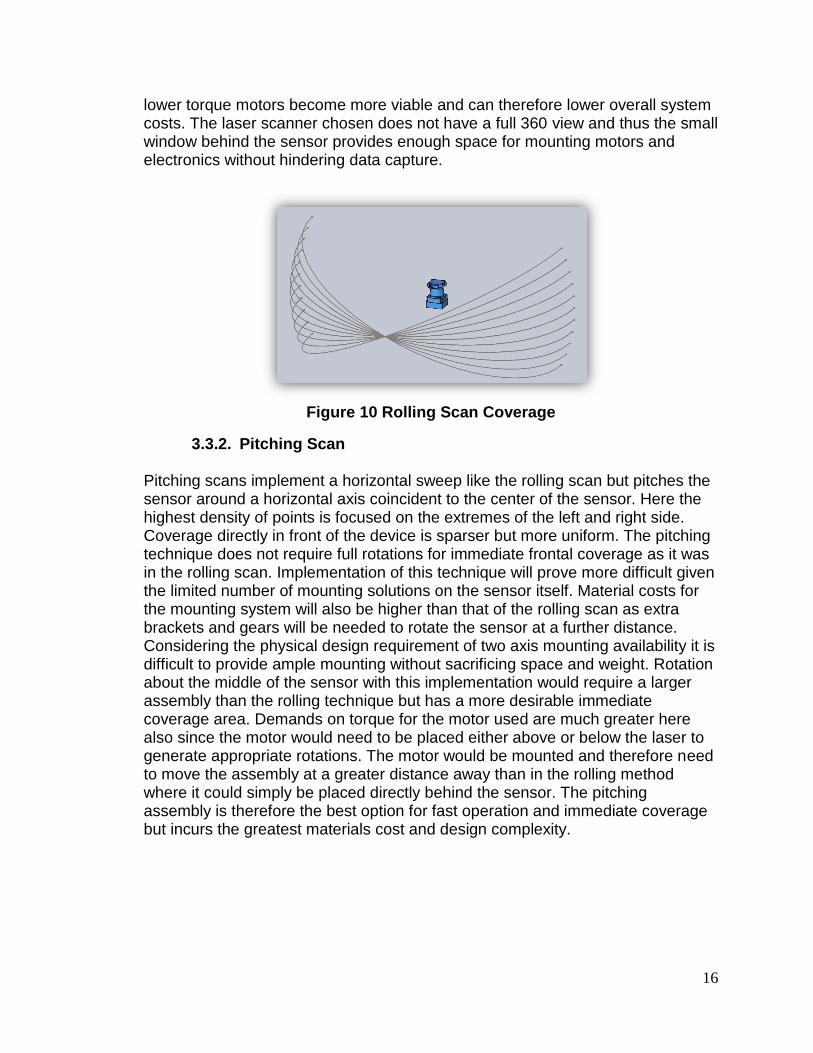
16

lower torque motors become more viable and can therefore lower overall system costs. The laser scanner chosen does not have a full 360 view and thus the small window behind the sensor provides enough space for mounting motors and electronics without hindering data capture.

Figure 10 Rolling Scan Coverage

3.3.2. Pitching Scan Pitching scans implement a horizontal sweep like the rolling scan but pitches the sensor around a horizontal axis coincident to the center of the sensor. Here the highest density of points is focused on the extremes of the left and right side. Coverage directly in front of the device is sparser but more uniform. The pitching technique does not require full rotations for immediate frontal coverage as it was in the rolling scan. Implementation of this technique will prove more difficult given the limited number of mounting solutions on the sensor itself. Material costs for the mounting system will also be higher than that of the rolling scan as extra brackets and gears will be needed to rotate the sensor at a further distance. Considering the physical design requirement of two axis mounting availability it is difficult to provide ample mounting without sacrificing space and weight. Rotation about the middle of the sensor with this implementation would require a larger assembly than the rolling technique but has a more desirable immediate coverage area. Demands on torque for the motor used are much greater here also since the motor would need to be placed either above or below the laser to generate appropriate rotations. The motor would be mounted and therefore need to move the assembly at a greater distance away than in the rolling method where it could simply be placed directly behind the sensor. The pitching assembly is therefore the best option for fast operation and immediate coverage but incurs the greatest materials cost and design complexity.

17

Figure 11 Pitching Scan Coverage

3.3.3. Yawing Scan The yawing scan utilizes a vertical sweep and implements a vertical axis of rotation central to the center of the sensor. There are two possible orientations of the sensor for coverage in this configuration with the laser either on its side or on its back. A sideways orientation is seen as more favorable for robotics as it can give the greatest immediate view to the platform. In applications requiring more than 180 degrees field of view this method would be the only viable option. To accomplish greater than 180 degree scans additional hardware would be required to manage a cables on a continuous rotating platform. Motor selection would also be limited to those capable of achieving this continuous state. Measurement densities of the yawing scan are heavily focused towards the top and bottom with greater uniformity around the circumference of the scan. Operation of the yawing scan closely resembles that of the pitching scan except that the rotation controls the horizontal field of view rather than the vertical. Construction of a rotating assembly for this technique has a difficulty between that of the pitching and rolling schemes with a cost reflecting that. With the sensor on its side or back the rotating apparatus can be built without significantly occluding the laser because of the window on the back of the sensor. Without the need for additional hardware, mounting flexibility of such a device would be more dynamic than in the pitching scheme. Numerous potential applications of this sensor make selection of the horizontal rather than the vertical field of view favorable because resolution is more easily relinquished for faster 3D imaging.

18

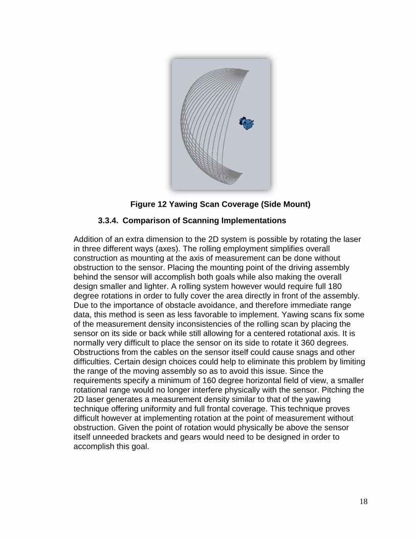
Figure 12 Yawing Scan Coverage (Side Mount)

3.3.4. Comparison of Scanning Implementations Addition of an extra dimension to the 2D system is possible by rotating the laser in three different ways (axes). The rolling employment simplifies overall construction as mounting at the axis of measurement can be done without obstruction to the sensor. Placing the mounting point of the driving assembly behind the sensor will accomplish both goals while also making the overall design smaller and lighter. A rolling system however would require full 180 degree rotations in order to fully cover the area directly in front of the assembly. Due to the importance of obstacle avoidance, and therefore immediate range data, this method is seen as less favorable to implement. Yawing scans fix some of the measurement density inconsistencies of the rolling scan by placing the sensor on its side or back while still allowing for a centered rotational axis. It is normally very difficult to place the sensor on its side to rotate it 360 degrees. Obstructions from the cables on the sensor itself could cause snags and other difficulties. Certain design choices could help to eliminate this problem by limiting the range of the moving assembly so as to avoid this issue. Since the requirements specify a minimum of 160 degree horizontal field of view, a smaller rotational range would no longer interfere physically with the sensor. Pitching the 2D laser generates a measurement density similar to that of the yawing technique offering uniformity and full frontal coverage. This technique proves difficult however at implementing rotation at the point of measurement without obstruction. Given the point of rotation would physically be above the sensor itself unneeded brackets and gears would need to be designed in order to accomplish this goal.

19

3.3.5. Open Loop Control In an open loop control system, only the current state and input are taken into account when driving the system. This control system is typically used in simple processes, as there is no feedback to see if the output matches the intended goal. In the following section, we discuss the viability of an Open Loop Control system for this project by taking into account each subsystem and the information it receives and transmits. As the most critical part of the project, the LIDAR unit must be considered first. In terms of input and output, the LIDAR units we have researched are almost identical and will therefore be discussed as a whole instead of individually. The main purpose of a LIDAR unit is to sweep an area with a laser, find a distance and transmit to whatever is listening. This is done without any response from the listening device. Each 360 degree rotation of the LIDAR takes a specific amount of time, making it possible for LIDAR and motor to work in tandem without the need for a sync pulse. While the LIDAR can be configured to only scan certain areas by changing the scan start angle and scan end angle, these settings are not modified while the system is in use. Given that any input to the LIDAR is set prior to actively using the device, it is entirely possible for a LIDAR unit to exist in an open loop control system as it needs no feedback. Next, we examine the unit that turns the 2D planes acquired by the LIDAR into a full 3D image, the motor. As there are several categories of motor we consider for this project; Stepper motors, Servo motors and DC motors with encoders; we will discuss them by their categories instead of motors as a whole. The stepper motor is capable of taking an dividing circular rotation into a specified number of steps, thus able to rotate at a constant distance per step. This is done with a number of electromagnets on the outer rim of the motor. To drive this motor, each electromagnet is given power in sequence to cause motion. As such, this fits well with the concept of an open loop control system as the motor is able to create a desired output given only its current state and correct input. A stepper motor can be programmed to repeatedly move from a start angle to an end angle at a predetermined rate, allowing for more than enough time for a LIDAR sweep at each step. A servo motor is a good example of the type of motor that is not usable in an open loop control system. Servo motors operate using feedback to correct performance, constantly monitoring mechanical position. This type of motor is perfect for a closed loop control system, and it is discussed length in the following section. DC motors operate by electrically charging a rotating armature inside of a magnetic field, thus controlling the speed of the rotations by the current supplied to the armature. A DC motor is a strong choice for projects requiring a large amount of torque or speed, as they can be started at high power by supplying a large amount of impedance with the DC voltage. As DC motors move at a rate relative to the impedance, an encoder must be added for there to be any capability for specific motion. An encoder converts the position of a motors shaft

20

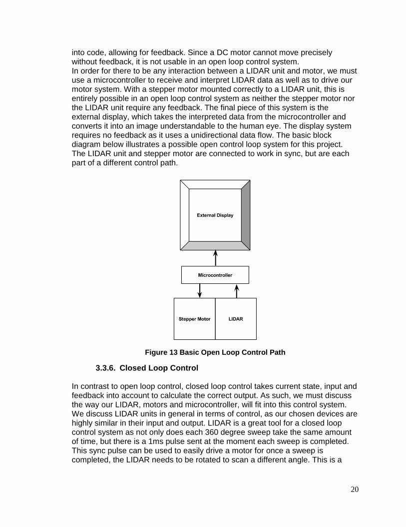
into code, allowing for feedback. Since a DC motor cannot move precisely without feedback, it is not usable in an open loop control system. In order for there to be any interaction between a LIDAR unit and motor, we must use a microcontroller to receive and interpret LIDAR data as well as to drive our motor system. With a stepper motor mounted correctly to a LIDAR unit, this is entirely possible in an open loop control system as neither the stepper motor nor the LIDAR unit require any feedback. The final piece of this system is the external display, which takes the interpreted data from the microcontroller and converts it into an image understandable to the human eye. The display system requires no feedback as it uses a unidirectional data flow. The basic block diagram below illustrates a possible open control loop system for this project. The LIDAR unit and stepper motor are connected to work in sync, but are each part of a different control path.

Figure 13 Basic Open Loop Control Path

3.3.6. Closed Loop Control In contrast to open loop control, closed loop control takes current state, input and feedback into account to calculate the correct output. As such, we must discuss the way our LIDAR, motors and microcontroller, will fit into this control system. We discuss LIDAR units in general in terms of control, as our chosen devices are highly similar in their input and output. LIDAR is a great tool for a closed loop control system as not only does each 360 degree sweep take the same amount of time, but there is a 1ms pulse sent at the moment each sweep is completed. This sync pulse can be used to easily drive a motor for once a sweep is completed, the LIDAR needs to be rotated to scan a different angle. This is a

21

very important fact, as this pulse can be used to drive multiple events in different systems. LIDAR units do not take in any feedback, however. The stepper motor is the perfect motor for an open control system as it provides a guaranteed motion given power to its electromagnets in the correct sequence. While this is a strong trait in any motor, in a closed loop control system feedback is necessary. It is possible to add an encoder to the stepper to measure the shaft location and ensure perfect angular rotation to allow for feedback, but this is overkill. While a stepper motor allows for perfect scan data storage as each step is the same distance, without proper feedback it is not a viable option in a closed loop control system. The servo motor typically operates by taking feedback on either the position or speed of the motor using an encoder. This is perfect for a closed loops system, as it allows us to continually have information on the location of motor, and the location of the LIDAR unit mounted to it. The servo motor is used in the basic closed loop control system detailed at the end of this section. A DC motor operates using a rotating armature inside of a magnetic field, where the speed of the motor can be controlled by the amperage provided to the armature. As such, there is no inherent control over the motors location. To fix this problem, an encoder is typically added to send feedback on the position of the motor shaft. A DC motor is a viable choice within a closed loop control system, although the method in which it rotates is less than opportune for the type of motion we will require for LIDAR operation. As in the open loop control system, the microcontroller is the core unit of this project. It is impossible to use the other subsystems without a controller, as the controller drives the motors, while taking in and interpreting LIDAR data before sending it to the external display system. LIDAR position feedback is provided through either a servo or DC motor with encoder, allowing for the LIDAR scan data to be stored with respect to current motor location. The external display system typically reads computed LIDAR data from the microcontroller and interprets it in a way that allows the human eye to understand the distances it has recorded. Usually the microcontroller and display system each interpret data independently, once the microcontroller has finished its computations they are sent to the display for it to begin translating distance into color. Since the display is doing calculations of its own, it is possible for errors to arise or for data to be missing. As such the display can request feedback from the microcontroller for a scan still in memory. A basic block diagram for the LIDAR system is shown below in figure 14. It shows the flow of data to and from the microcontroller, as well as the feedback for each subsystem. Note the LIDAR unit does not receive feedback, but instead transmits data as well as a sync pulse for timing.

22

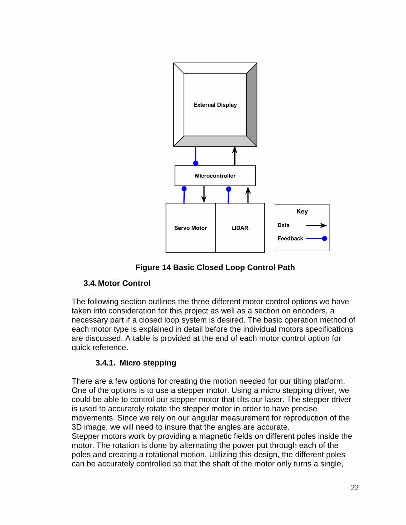
Figure 14 Basic Closed Loop Control Path

3.4. Motor Control The following section outlines the three different motor control options we have taken into consideration for this project as well as a section on encoders, a necessary part if a closed loop system is desired. The basic operation method of each motor type is explained in detail before the individual motors specifications are discussed. A table is provided at the end of each motor control option for quick reference.

3.4.1. Micro stepping There are a few options for creating the motion needed for our tilting platform. One of the options is to use a stepper motor. Using a micro stepping driver, we could be able to control our stepper motor that tilts our laser. The stepper driver is used to accurately rotate the stepper motor in order to have precise movements. Since we rely on our angular measurement for reproduction of the 3D image, we will need to insure that the angles are accurate. Stepper motors work by providing a magnetic fields on different poles inside the motor. The rotation is done by alternating the power put through each of the poles and creating a rotational motion. Utilizing this design, the different poles can be accurately controlled so that the shaft of the motor only turns a single,

23

constant, distance. This allows stepper motors to be controlled to turn degree by degree. The cost of the stepper is attractive due to its lower cost. One downside, however, to using the stepping controller is that the stepper and driver do not provide feedback to our system.

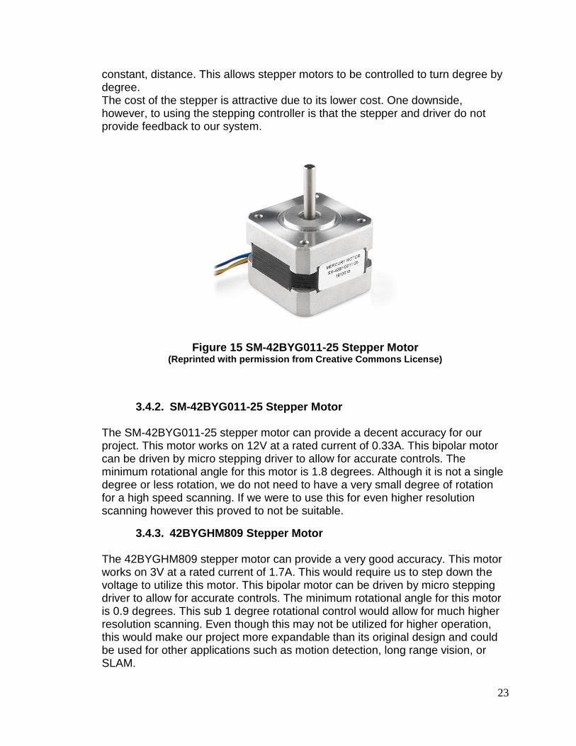
Figure 15 SM-42BYG011-25 Stepper Motor

(Reprinted with permission from Creative Commons License)

3.4.2. SM-42BYG011-25 Stepper Motor The SM-42BYG011-25 stepper motor can provide a decent accuracy for our project. This motor works on 12V at a rated current of 0.33A. This bipolar motor can be driven by micro stepping driver to allow for accurate controls. The minimum rotational angle for this motor is 1.8 degrees. Although it is not a single degree or less rotation, we do not need to have a very small degree of rotation for a high speed scanning. If we were to use this for even higher resolution scanning however this proved to not be suitable.

3.4.3. 42BYGHM809 Stepper Motor The 42BYGHM809 stepper motor can provide a very good accuracy. This motor works on 3V at a rated current of 1.7A. This would require us to step down the voltage to utilize this motor. This bipolar motor can be driven by micro stepping driver to allow for accurate controls. The minimum rotational angle for this motor is 0.9 degrees. This sub 1 degree rotational control would allow for much higher resolution scanning. Even though this may not be utilized for higher operation, this would make our project more expandable than its original design and could be used for other applications such as motion detection, long range vision, or SLAM.

24

3.4.4. A3967 Micro stepping Driver The A3967 micro stepping driver is controlled using a high pin for stepping and a high pin for direction. It will run off of our 12V power rail in order to power. It can also operate up to 750mA. The motor hooks up to the driver using 4 wires, A & B in and A & B out. These correspond with the 2 phases in the stepper motor and control the stepper motor motion. We would be developing the software that controls the stepping of the motor in this case. This driver works on the rising edge of a controlled clock that corresponds directly with the motor control. It does not utilize a serial system for control or feedback. Therefore, we would need to manage the step counting within our program.

3.4.5. STMicro's L6470 Stepper Motor Driver The STMicro's L6470 stepper motor driver is more robust driver than the A3967. The L6470 can operate in the range of 8-45V, which includes our 12V rail and can operate up to 3A. This would provide the ability to have a much larger power motor. Communicating to the stepper controller is done using an SPI link. This serial link is more stable and allows for full duplex operating. This means that we can send it commands to move as well as get feedback returned to us about its operating modes, speed, and location. It manages this information using registers onboard the driver. Utilizing this driver may prove beneficial for us for stability; however, we will also have to take into account the additional points of failure that could occur. Because this driver uses the SPI interface, we would need to have a specialized clock signal for communication. This takes away from our existing number of pins and may require us to utilize additional shift registers. This could lead to delays and possible failures.

3.4.6. Servo The other option is to use a servo. The servo moves differently than the stepper as it is a more fluid movement and it will rotate until it has reached its position. This can lead to slipping and inaccurate results. However, servos will provide location feedback by using an encoder in order to provide the exactly location down to the degree. This allow for an extremely accurate results since the movement is not geared and depends on the encoder resolution used. Most servos, however, do not allow for full rotation and can only alternate direction within a limited range. This is fine for our application since we will be unable to rotate a full 360 degrees.

25

Figure 16 Hitec HS-805BB Servo Motor


3.4.7. Hitec HS-805BB Servo Motor The Hitec HS-805BB servo motor provides 180 degrees of rotation. This servo motor works on 6V, so the voltage will have to be stepped down from our 12V rail. The maximum operating current of the servo is 800mA. This servo can provide 343 Oz-in of maximum torque, so moving the laser mechanism would not be an issue.

3.4.8. Dynamixel MX-28T Robot Actuator The Dynamixel MX-28T Robot Actuator is another such servo that can provide an accurate movement. It requires serial communication to send it position data and also to receive position data back from the servo. It uses a potentiometer in order to provide the encoded position information. This servo provides a resolution of 0.088 degrees. This level of accuracy would allow for our application as well as the numerous others for high resolution 3D scanning. This servo also has 360 degrees of rotation to allow for a full field of vision. This servo has a built in driver that allows for the serial communication. It monitors the position, the load, the input voltage, and the temperature. The communication speed can be adjusted between 7343 bps to approximately 3Mbps. After testing we found that we were able to utilize the highest speed for communication with little error. This servo works on 12V and has a maximum operating current of 2400mA. Using this amount of power would require us to make some sort of protection circuit that is more robust than other motors may have required, but was worth it since this gave the most options.

26

3.4.9. DC Motor Control DC motors allow you to provide an amount of regulated power to move a specific distance. This is done by rotating a charged armature in a magnetic field, where the speed is dependent on the amount of current provided. These types of motors are extremely cheap, but they are not accurate. The DC would prove viable if an encoder and/or limit switches are used.

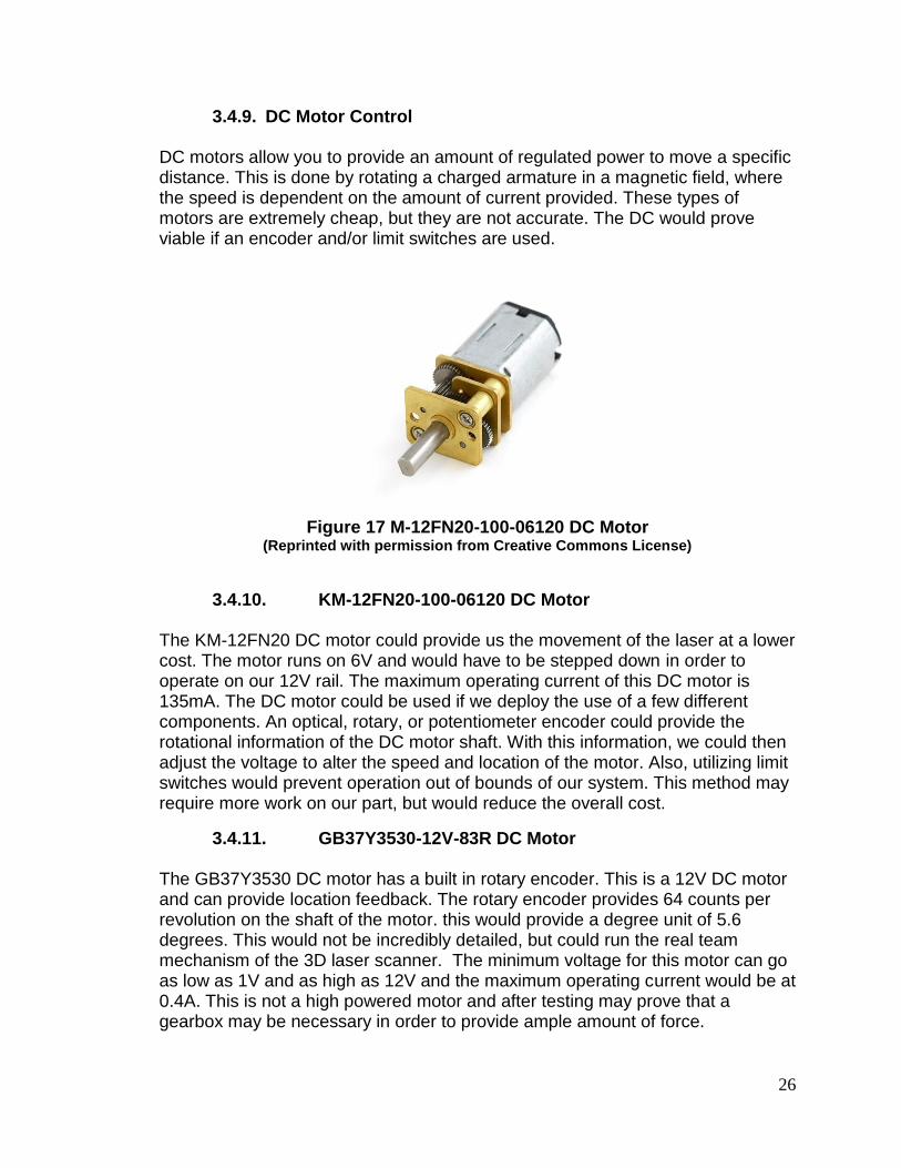
Figure 17 M-12FN20-100-06120 DC Motor


3.4.10. KM-12FN20-100-06120 DC Motor The KM-12FN20 DC motor could provide us the movement of the laser at a lower cost. The motor runs on 6V and would have to be stepped down in order to operate on our 12V rail. The maximum operating current of this DC motor is 135mA. The DC motor could be used if we deploy the use of a few different components. An optical, rotary, or potentiometer encoder could provide the rotational information of the DC motor shaft. With this information, we could then adjust the voltage to alter the speed and location of the motor. Also, utilizing limit switches would prevent operation out of bounds of our system. This method may require more work on our part, but would reduce the overall cost.

3.4.11. GB37Y3530-12V-83R DC Motor The GB37Y3530 DC motor has a built in rotary encoder. This is a 12V DC motor and can provide location feedback. The rotary encoder provides 64 counts per revolution on the shaft of the motor. this would provide a degree unit of 5.6 degrees. This would not be incredibly detailed, but could run the real team mechanism of the 3D laser scanner. The minimum voltage for this motor can go as low as 1V and as high as 12V and the maximum operating current would be at 0.4A. This is not a high powered motor and after testing may prove that a gearbox may be necessary in order to provide ample amount of force.

27

3.4.12. Encoders Encoders provide feedback of a motor to a circuit. Encoders are used to monitor the motion of the motor’s shaft and provide a method that reports feedback of that motion. We will need to discuss which of the encoders we will use if we decide to use a DC motor in our application. Even though servos come with motor feedback, there may be a need for a redundant system to measure and test the given motor feedback.

Figure 18 E6A2-CS3E Rotary Encoder


3.4.13. E6A2-CS3E Rotary Encoder This rotary encoder allows us to attach it to any motor and provide motor feedback. This type of rotary encoder uses a potentiometer to measure motion. It works on between 5V and 12V, so it would be able to use our main 12V rail. The maximum revolution per minute is 5000rpm. The feedback is provided by voltage levels. This would require us to write the code in our main application, or to create a separate board just for handing the information.

3.4.14. A6B2-CWZ3E-1024 Rotary Encoder This rotary encoder provides feedback of the shaft of a motor using a different method than the previous encoder. This uses light in order to sense the motion of the motor shaft. This is encoder is called an optical encoder. It uses a disc that passes between a light and a sensor to sense the amount of rotation on the shaft of the motor. This encoder provides a resolution of 1024 light pulses per revolution. This equates to a 0.35 degree accuracy of motor rotation. This encoder works between 5V and 12V, so it will be able to run off of our 12V power rail.

28

3.4.15. Comparison of Motors Each of the motors that we have discussed has the ability to provide the function we need. We chose the type of motor that we will use in order to provide our motion. We needed the motion to be consistent and reliable in order to provide the scan. The DC motor will allow us to variably control speed and direction. This would be good at providing the fluid motion. However, accurate motion may not be easily acquired. The DC motor may hang if the weight of the laser scanner and platform and then the angle at which the tilt of the laser may not be constant. This could be remedied using a form of encoder. The stepper motors could also provide us the motion of the laser mechanism. Steppers can provide an accurate method of motion and can be controlled down to less than a single degree. Having the ability to get accurate movement is crucial to our calculations. However, the stepper motors do something that may not allow us to use them: they tick. Since the motor is controlled by telling each internal coil to electrify a certain amount, the motor actually does this by being fed many small values. This movement creates an unfavorable motion that is not smooth. It may be possible to use a motor controller to provide small enough ‘ticks’ to give the illusion of fluid motion. Nevertheless, this was a possibility and it could provide accurate motion for our system. The servo will provide us a fluid movement much like the DC motor, however, the servo has a built in encoder. Servos are designed to be accurate. This will provide us with the fluid motion that is required to get accurate readings as well as being able to get feedback to verify the angle of the motor. The following table provides a compares the different motors that we have discussed.

Part # Hitec HS-805BB

Dynamixel MX-28T

SM-42BYG011-25

42BYGHM809 KM-12FN20-100-06120

GB37Y3530-12V-83R

Motor Type

Servo Servo Stepper Stepper DC DC

Feedback Yes Yes No No No No Controller

Needed No No Yes Yes Yes Yes

Interface Pulse Voltage

Serial Comm

Pulse Voltage

Pulse Voltage Direct Voltage

Direct Voltage

Resolution 1 0.088 1.8 0.9 ---- 5.6 Torque 2.42N-

m 2.54N-m 0.226N-m 0.48N-m 0.054N-

m 0.29N-m

Max Speed 0.14 sec/60°

0.079 sec/60°

---- ---- 120rpm 83rpm

Max Amps 0.8A --- 0.33A 1.7A 135mA 0.4A Voltage 4.8V -

6V 12V 12V 3V 2V - 6V 1V - 12V

Cost $39.95 $219.90 $14.95 $16.95 $15.95 $29.00 Table 3 Comparison Chart of Motors

29

3.5. Microcontrollers / Computing The system architecture and specifications laid out in the previous section assumes an advanced computing solution to allow the system to be as fully embedded as possible. Generating full depth images and publishing them over a networking framework requires the system have ample memory (RAM) footprints as well as retain certain hardware I/O requirements. Certain capabilities of the outlined system have assumed inclusion of powerful open source libraries traditionally available only on desktop operating systems. Writing specific implementations of the functions necessary for 3d data visualization and image processing are outside the scope of this project. This eliminates most of the traditional commercial market of simple 8 or 16 bit microcontrollers. With the advent of newer 32-bit ARM based microcontrollers/SOC’s the term microcontroller has evolved in recent years. Desktop like development in the embedded space is now possible while still retaining all of the normal advantages of price, size, and power. Unlike traditional development board offerings of the likes of Arduino, microchip, or TI’s Launchpad some modern single board computer offerings have the advantages of actually allowing development/debugging onboard. These systems are ideal for the scope of this project as many run full desktop operating systems to enable faster and more refined development solutions. Most systems run the Linux kernel under popular Linux distributions such as Debian, Arch, and Ubuntu. These new single board computers are the reasons that projects such, as the one proposed, are now possible. The intent of the proposed system is to alleviate some computation on the end robotics application. By embedding the computation necessary to control the pitch, scans, and end translations the saved resources will greatly increase total system response. Building a system with these capabilities outside of a full x86 architecture would prove difficult due to limitations on available system memory for storing scan data. Scans generated by the Hokuyo scanner come in at a rate of 40 Hz with 1080 points per scan. Each point can contain up to 4 bytes (64bit) of accuracy giving a total scan at this precision a size of at least 4320 bytes or just over 4 kilobytes (see SCIP 2.0 Hokuyo interface). Even utilization of the 2 character encoding (16bit) will still use over a kilobyte per single scan interval. Given an average 3D vertical scan range of 45 degrees with 1 degree resolution each 3D scan would involve at least 90 kilobytes of raw scan storage. Most traditional 8 and 16 bit microcontrollers provide memory footprints of around a couple kilobytes. Some higher end 32 bit arm models will offer up to a couple hundred kilobytes of RAM however this would only allow for minimum accuracies of 2D data which would hinder the systems intent of high precision. With the advent of newer ARM based SOCs memory footprints have increased into the range necessary for a small embedded application. Many new offerings have come into the market including the Panda board, Raspberry Pi, Beagle board, and others which offer complete computing solutions within the required memory footprint. These boards offer the desktop like development desired while also

30

retaining low level I/O. The small footprint of these offerings will allow for a more streamlined tilting assembly and lower system power consumption.

3.5.1. Raspberry Pi Released in early 2012 with lots of attention the Raspberry Pi is a small embedded computing platform with the design goal of bringing computing to students in all parts of the world. The two variants available of the Pi include a model A which has price of $25 which is outfitted with a 700 MHz ARM1176JZF-S ARM 11 processor featuring the ARMv6 ISA. With 256 MB of ram this computing platform is capable of running full Linux operating systems enabling developers anywhere to program for a small price. With a power rating of 300 mA and a size of 3.37 inches by 2.125 inches this microcontroller capable board carries with it a small footprint and a lot of i/o potential. With a total of 8 GPIOs (General Purpose Input Output) pins, I2C busses, and full 3.3v and 5v rails this is a great platform for embedded systems. A bump of ten dollars to $35 will purchase what is called the model b version which sports similar specifications to the model a version with a few extra connectivity options in the added Ethernet and USB ports. The increased price also comes from a doubling of RAM system wide to 512 MB which is of major appeal to a system looking at storing tens of thousands of points from laser scans. While the disadvantage to this variant is a doubling of power consumption to upwards of 700 mA the total consumption is still less than 5 W. This makes the model b Raspberry Pi a very viable microcontroller option for the 3D system and would enable a smaller system footprint given its near credit card footprint.

3.5.2. Beagle Board Black Similar to the Raspberry Pi, the Beagle Board Black is a low cost embedded computing solution, although a slightly higher cost. The board has a cost of $45, with a 1GHz TI Sitara AM3359 ARM Cortex A8 processor. With 512 MB of 400MHz DDR3L RAM and a built in 2GB of storage, the Beagle Bone is able to run a multitude of different Linux versions. It uses more power than the Raspberry Pi A but less than the B, drawing from 210-460 mA depending on conditions of use, although it is almost the same size at 3.4” by 2.1”. It has a large amount of GPIO pins, with 65 pins available, and has both 3.3v and 5v rails. Unlike the raspberry pi, the only display option available is HDMI with audio. During the project we will be using our chosen board as an embedded system, so the single video output does not affect the board too heavily. The Beagle Board Black is a good step up from the Raspberry Pi in terms of speed, RAM and storage for the same size board.

3.5.3. Panda Board ES The Panda board ES represents a higher end model for an embedded controller, as the newest model is currently $182, although the higher price is not unjustified. The Panda board ES comes with a Dual-core 1.2GHz ARM Cortex-

31

A9 MPCore with SMP processor, which is a large step up from the raspberry pi and beagle bone with double the processing power. It also comes with a whopping 1GB or DDR2 RAM and an Imagination Technologies’ POWERVR SGX540 384MHz graphics core, which supports multiple OpenGL libraries and assists in image processing. The device has the largest physical footprint of all choices at 4.5” by 4”, with the most internal components as well. Unlike any of our other choices, the panda board has a built in Texas Instruments WiLink 6.0 Module with 802.11 b/g/n and Bluetooth support which can be used to transmit data wirelessly to an external device, such as an Android smartphone running OpenCV to display our depth-images. As the Panda board EX supports Android and Ubuntu, this would allow for us to use very similar software architecture between devices. There are no GPIO pins built into the device, though the Generic Expansion Connectors allow for us to add pins if necessary. The device runs on a 5V DC connection and has a maximum power rating of 800mA and a minimum power rating of 170mA. The Panda board ES is a very powerful microcontroller, albeit a bit large and pricey.

3.5.4. Comparison of Microcontrollers In order to compare the three microcontrollers we outlined in the previous section, we must first decide how to compare them. The most important factors to our project are overall clock-speed, available data storage space, power usage and size of the microcontroller. The following section discusses each point respectively. The fastest board researched is the Panda Board ES, with its impressive Dual-Core 1.2GHz ARM Cortex-A9, it is over twice powerful as any other microcontroller we have taken into consideration. On the Single-Core side of our choices, we have the Raspberry Pi model B and the Beagle Board Black. Both boards are inexpensive compared to the Panda board EX, with the Raspberry Pi ($35) only beating the Beagle Board Black ($45) by 10 dollars. The two boards are close in processor power, Beagle Board’s 1GHz TI Sitara AM3359 ARM Cortex A8 is only 300MHz stronger than the Raspberry Pi’s 700MHz ARM1176JZF-S.While both boards provide a decent clock speed for our project, a dual-core microcontroller is in a class of its own. Given the speed at which our LIDAR sensor will be sending large packets of data, a higher processor speed is very important for us to be able to view the information in real time without errors. However, a multi-core processor requires pipelined instructions in order to reach its maximum efficiency, which are more complicated in nature than those of a single-core processor. The Panda board ES is our highest microcontroller price point available, at over three times the price of the Beagle Board Black and over five times the price of the Raspberry Pi model B. Given the amount of data we will need to keep stored for quick access, our total RAM available is an important factor. The majority of data received from the LIDAR sensor will be stored in RAM, as will the results of any computations on said data; therefore it is well advised that we have enough RAM to store multiple

32

scans, as well as their visual representations. The Panda Board ES has the most RAM with 1GB, with the Raspberry Pi model B and Beagle Board Black having an available 512MB. While the amount of RAM is important to our incoming data and computation resultant storage, space is still needed for a basic operating system and our LIDAR code. The Beagle Board Black stands out in this situation, as it has 2GB of internal storage and a SD/MMC slot for external storage. Neither the Panda Board ES nor the Raspberry Pi have any internal storage, and require a SD card for their operating system and code space. While this seems like quite a hindrance, fast class 10 SD cards are available up to 64GB, which is far more than we will need and thus not a large issue overall. In terms of size, the Raspberry Pi and Beagle Board Black combined are still smaller than the Panda board ES. The Beagle Board Black is the smallest board, at only 3.4 inches by 2.1 inches it takes up only 7.14 inches2. The Raspberry takes an incredibly close second at 3.37 inches by 2.125 inches, it’s 7.16125 inches2 area is only two tenths of a square inch larger, an almost insignificant amount. The two boards allow for the project to be as minimal in area as possible, as it is intended for a robot with specific size limitations. At 4.5” by 4” the Panda board ES is larger than either board, with more than double the overall area than its competition at 18 inches2 used. Between the three boards, the Panda board ES’s multitude of features cause it to take up a large physical area, which is a disadvantage in our project. Finally, we discuss power usage. While all three boards are compatible with 5V DC power supply, only the Raspberry Pi and Beagle Board Black are able to use a 3.3V DC power supply. Since we plan to use a 5V DC supply, the alternative power option is not necessary, though a welcome addition if a lower power rating is needed. Between the three boards, the Panda board ES draws the most current, with a maximum of 800mA at full usage. Once again, the Raspberry Pi and Beagle Board Black are close in specifications, where the Raspberry Pi model B has a maximum draw of 700mA and the Beagle Board draws a maximum of 470mA.

33

All of the specifications discussed in 3.5 Microcontrollers/Computing are condensed into the table below.

Raspberry Pi Model B

Beagle Board Black

Panda Board ES

Price $35 $45 $182

Processor 700MHz 1GHz 1.2GHz Dual Core

RAM 512MB 512MB 1GB

Storage SD/MMC Slot SD/MMC Slot 2GB internal, SD/MMC Slot

Size 3.37” x 2.125” 3.4” x 2.1” 4.5” x 4”

Power Supply

3.3V DC or 5V DC 3.3V DC or 5V DC 5V DC

Max. Drain 700mA 470mA 800mA

Table 4 Comparison Chart of Microcontrollers

3.6. Power Regulated power to all components in the system is crucial for smooth and consistent operation. Input into the system could potentially be provided by multiple sources on the robotic platforms including shore power based systems or logic/motor battery systems. When the systems are not undergoing testing in the field the system will be powered by either a 12V or 24V DC system. This shore powered system consists of AC to DC converters as well as DC to DC converters to 12V. This system allows for the option of plugging the entire robotic platform into the wall to keep all essential systems online without the requirement of the batteries. This allows for the batteries to be charged while development can continue onboard the system. The same is to be true of the embedded LIDAR system to be developed. In order to properly ascertain power management of the system it is expected that total system consumption be less than 36 Watts total. The breakdown of the total expected system consumption can be seen in the table below.

Component Expected Voltage (Volts V)

Average Current (Amps A)

Average Power (Watts W)

LIDAR 12.0 0.75 9.0

Motor 12.0 1.25 15.0

Microcontroller 5.0 0.75 3.75

Encoder 5.0 0.10 0.5

Webcam 5.0 0.5 2.5

Total Expected Power Consumption 30.75

Table 5 Expected Power Consumption by System Component

34

With an average of 30.75 Watts predicted for the system the goal maximum load of 36 Watts is well within reach. Proper testing of each physical component will be necessary for proper power consumption approximation as each component is manufactured to different tolerances and will use varying amounts than specified from the manufacturer.

3.6.1. Regulation There are different topologies available to convert the 12-24V DC input into the system down to the 3.3 and 5V logic necessary for the smaller system components. The two most commonly used regulators are linear and switching based voltage regulators. Each type has many different advantages and disadvantages based upon the intended application. With the goal of maximizing regulator and total system efficiency it is necessary for the group to choose the best methodology for regulation. Other factors which will be considered by the group in choosing the best regulator includes the criteria of input/output voltage ranges, thermal output, package type, footprint size, and external componentry. Linear based regulators can only step down output voltage from the input whereas switching systems can step up, down, or invert. Efficiency of linear solutions is typically lower than that of switching where the difference between the input and output voltages to the system are great. This would be the case in this system where the minimum input and output voltages would be 12V and 5V respectively. It is also a requirement of linear systems that the input current be the same as the output current which typically causes lots of heat on the regulator itself. This is a characteristic that is not shared in switching regulators and is another characteristic of linear design that must be considered when designing a PCB. However the tradeoffs towards implementation of a switching system typically include higher complexity in terms of external componentry. Switching systems can call for the use of many diodes, inductors, and filtering capacitors before input can be received by the integrated circuits. This contrasts heavily to the common linear system where the only external components are usually simple bypass capacitors. The linear systems also do not frequently experience the kinds of noise and ripple associated with switching systems. This is highly dependent on the switching rate of the given regulator however and is not normally a complication. Comparing both linear and switching regulation technologies it is hard to determine exactly which technology will be used in the final system. The group therefore decided it would be best to examine products from both categories to determine the proper integration for the system.

3.6.2. TI LMZ14203 Simple Switcher The LMZ14203 switching power module is a step-down based switching regulator solution. The part has been found capable of driving a 3A load which is sufficient for our power requirement of 6.75 Watts on the 5V rail as demonstrated in table 5. The IC is capable of handling from 6V to 42V maximum and is available in a TO-PMOD-7 package. This package type has 7 large pins all

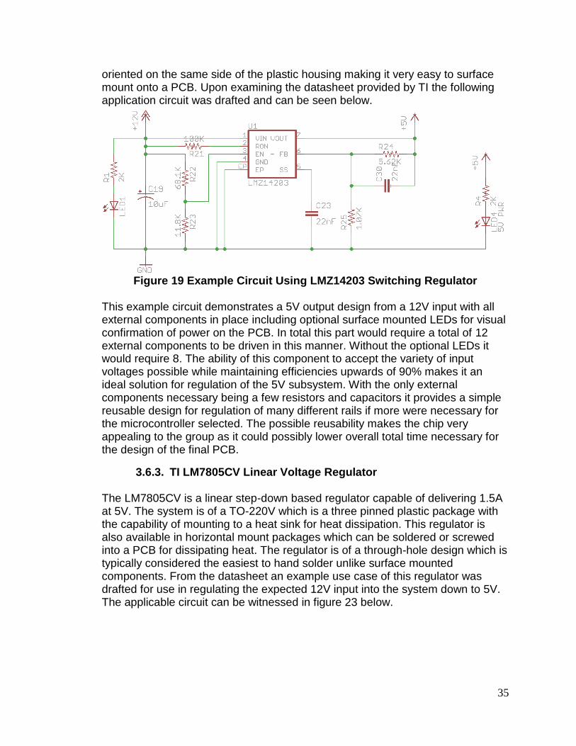
35

oriented on the same side of the plastic housing making it very easy to surface mount onto a PCB. Upon examining the datasheet provided by TI the following application circuit was drafted and can be seen below.

Figure 19 Example Circuit Using LMZ14203 Switching Regulator

This example circuit demonstrates a 5V output design from a 12V input with all external components in place including optional surface mounted LEDs for visual confirmation of power on the PCB. In total this part would require a total of 12 external components to be driven in this manner. Without the optional LEDs it would require 8. The ability of this component to accept the variety of input voltages possible while maintaining efficiencies upwards of 90% makes it an ideal solution for regulation of the 5V subsystem. With the only external components necessary being a few resistors and capacitors it provides a simple reusable design for regulation of many different rails if more were necessary for the microcontroller selected. The possible reusability makes the chip very appealing to the group as it could possibly lower overall total time necessary for the design of the final PCB.

3.6.3. TI LM7805CV Linear Voltage Regulator The LM7805CV is a linear step-down based regulator capable of delivering 1.5A at 5V. The system is of a TO-220V which is a three pinned plastic package with the capability of mounting to a heat sink for heat dissipation. This regulator is also available in horizontal mount packages which can be soldered or screwed into a PCB for dissipating heat. The regulator is of a through-hole design which is typically considered the easiest to hand solder unlike surface mounted components. From the datasheet an example use case of this regulator was drafted for use in regulating the expected 12V input into the system down to 5V. The applicable circuit can be witnessed in figure 23 below.

36

Figure 20 Example Circuit Using the TI LM7805CV

The three pinned regulator only requires a couple of bypass capacitors making the footprint of this regulation system extremely simple. In total this regulation system would only require a total of 3 components and two of those are just bypass capacitors making it ideal for reducing PCB footprint size. On higher loads however it may be necessary to add a mounted heat sink or add a screw mount to the board in order to dissipate the extra heat that can be generated on higher loads. The LM series of linear regulators is very popular in small embedded projects because of their built-in over current protection which makes it impossible to draw too much power from them. This is partially due to the built in overheating protection which can regulate how much power can actually be drawn through the regulator at any given time. This can provide safety to the microcontroller and other components in the system running off the output rail generated by this regulator and makes for an appealing option. The price of this linear regulator is also much less than that of other more elaborates switching systems. This is another advantage if more regulators are needed throughout the system as repeatability will cost less as smaller BOM means a smaller PCB and a smaller overall cost.

3.6.4. CUIINC V78-2000 The goal of the CUI V78 series is to compete with the success of the TI LM78xx series linear regulators. An example of one of these regulators can be seen in the previous section. The V78 family is available in a similar package and can be dropped into the same footprint as the LM78 series regulators. These components however are not linear but instead are fully embedded switching

37

regulators similar to that of the LMZ series. The similarity to the LM78 regulators means the same circuit seen in figure 23 can be used with this IC. Just like the previous LM TI series the V78 needs only two bypass capacitors for normal operation making its foot print the exact same to that of the TI linear solution. The output of the V78-2000 is 2A at 2.5, 3.3, 5, or 6.5 volts. This is due mainly to the fact that it is a switching based regulator and thus the switching frequency can be modified to the require output voltages. This provides a lot of the same flexibility as the TI LMZ based switching regulator but with all of the advantages of a smaller linear solution. That is to say it also has a similar efficiency curve to match that of a normal switching system. There is a stricter limitation however on the available input voltage range being from 4.75-18v. Assuming a 12v input into the system however it is still well within tolerance. The overall smaller footprint also means that more components or additional regulators can be fit onto the PCB without sacrificing price which is not normally the case for a switching regulator. This makes the CUI V78 series an appealing option as it would appear to have all of the most important advantages of both linear and switching technologies without introducing any new drawbacks.

3.7. Waterproof Connectors As part of the project requirements and the expected operating environment of the proposed system it has been deemed necessary to isolate connections from the 3D laser system to the other components on the robotic platforms. This helps to ensure compatibility with current external connection systems which already exist frequently on the robots in the organization currently. It will also ensure operational safety to the individual components on both ends of the connection. At minimum the power lines should be protected from the elements as to ensure that no excess in humidity, condensation, or other forms of moisture are able to cause shorting across the DC inputs into the system. These inputs could be supplying upwards of 30 Watts at any given time and a short could cause catastrophic failure to other systems tied into that input if a short were to occur. Waterproof connectors will also provide an easy way to disconnect and reconnect the system in a regular fashion as will be necessary moving the system across multiple platforms.

3.7.1. Weipu Connectors Running power to and from the boxes and enclosures of the various robots to the embedded LIDAR platform requires a safe interface which can withstand a variety of different weather conditions. Attempting to achieve the NEMA standard of IP45 or better requires a minimum level of waterproofing. Finding a series of connectors with multiple footprints, connector ratings, and multiple conductors is a vital aspect of a successful embedded LIDAR solution.

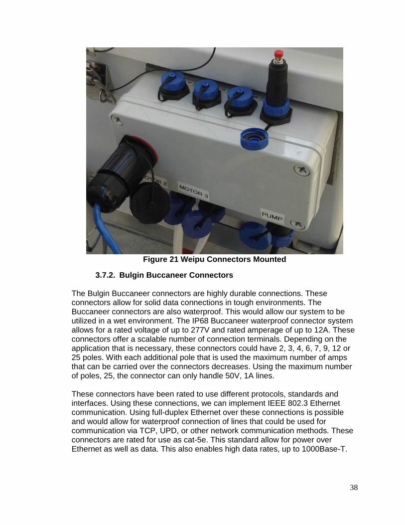
38

Figure 21 Weipu Connectors Mounted

3.7.2. Bulgin Buccaneer Connectors The Bulgin Buccaneer connectors are highly durable connections. These connectors allow for solid data connections in tough environments. The Buccaneer connectors are also waterproof. This would allow our system to be utilized in a wet environment. The IP68 Buccaneer waterproof connector system allows for a rated voltage of up to 277V and rated amperage of up to 12A. These connectors offer a scalable number of connection terminals. Depending on the application that is necessary, these connectors could have 2, 3, 4, 6, 7, 9, 12 or 25 poles. With each additional pole that is used the maximum number of amps that can be carried over the connectors decreases. Using the maximum number of poles, 25, the connector can only handle 50V, 1A lines. These connectors have been rated to use different protocols, standards and interfaces. Using these connections, we can implement IEEE 802.3 Ethernet communication. Using full-duplex Ethernet over these connections is possible and would allow for waterproof connection of lines that could be used for communication via TCP, UPD, or other network communication methods. These connectors are rated for use as cat-5e. This standard allow for power over Ethernet as well as data. This also enables high data rates, up to 1000Base-T.

39

Firewire and USB2.0 interfaces are supported via these connectors as well. With these connectors, the host system can communicate with USB peripherals in a waterproof environment. USB2.0 provides high speed serial data communication. This could allow for multiple component communication through this single connector. USB2.0 supports a maximum of 480Mbps throughput. This speed will be split up between communications for each device that is shared on the same bus. The connectors feature multiple safety features that prevent accidental connections and potential catastrophic scenarios. The connectors feature screw on caps that are keyed in a certain way to make sure that the connection cannot be mistaken. The caps do not require tools to connect either. Using tools could potentially create too much force on the connections and would possibly allow for stripping of the connections. Only allowing hand-tightened connections keeps the possibility of damaging the connections at a minimum. These connectors also feature a number of O-rings prevent leakage and maintain the constant pressure to remain secure. There is also a gland and a gland nut that keep the water from entering the electrical areas of the connector. All of these precautions will allow the connector to remain dry and operate as a normal connection would. The cost of these connectors may be limiting on a large scale, but for a small scale project, they would be fine. As well as waterproof, these connections advertise themselves as dust proof. Many military applications require use of electronics in the desert. The desert can lead to corrosive and deteriorating environments that would otherwise destroy electrical connections. Using these connectors, the sand and water would not reach the electrical components and allow for a much longer and safer lifespan for the systems involved.

40

Table 6 Bulgin Buccaneer Connectors

3.8. Data Representation Software A point cloud is a 3-dimensional representation of space. It includes an X, Y, and Z plane. This can include single or multiple objects.

Figure 22 Point Cloud Image

(Permission granted by PCL)

We are using point clouds to represent our environment in front of our sensor. We are collecting information from our laser sensor and then creating our point cloud on the fly. Although point clouds represent 3D objects and environments, they are merely a snapshot of the world. In order to utilize the point cloud the information held within must be manipulated and processed to be usable. The use of object recognition or surface recognition may have to be utilized in order

41

to see an actual surface. Representing the information will require the use of 3D rendering software. This software will display using the given coordinates, X, Y, and Z. Some current software such as Autodesk AutoCAD, will take this information and use detection algorithms in order to differentiate between different objects and surfaces. A very powerful library for the use and manipulation point clouds is the Point Cloud Library or PCL. The Point Cloud Library is a standalone, large scale, open project for 2D/3D image and point cloud processing. Since March 2011, the site has been devoted to the mapping of 3D image representation and creation. This library contains many modules: filters, features, registrations, kdtree, segmentation, sample consensus, range image, keypoints, octree, surface, visualization, and IO. Each of these modules gives high level access to functions and methods below them. The module that may interest us the most for our project is the Range Image module. The pcl_range_image library contains two classes for representing and working with range images. A range image (or depth map) is an image whose pixel values represent a distance or depth from the sensor's origin. Range images are a common 3D representation and are often generated by stereo or time-of-flight cameras. With knowledge of the camera's intrinsic calibration parameters, a range image can be converted into a point cloud. Another module that will help us in our project is the IO module. The pcl_io library contains classes and functions for reading and writing point cloud data (PCD) files, as well as capturing point clouds from a variety of sensing devices. Using this library in conjunction with the API provided by our laser sensor, we may be able to create a dynamically changing point cloud that we can represent. A third module that we can use is the visualization module. The pcl_visualization library was built for being able to quickly prototype and visualizes the results of algorithms operating on 3D point cloud data. This will allow us to assemble the point cloud library in order to view it. This is not necessarily needed for the core function of the application, but is needed for debugging and human interaction.

3.8.1. Depth Imaging Sometimes you cannot choose the optimum angle to take a picture. If the object is essentially planar (e.g. a painting on a wall) or the angle is not off by much then there is hope that you can correct the perspective afterwards. This is highly the case in our project, where we will be accessing an angular view of the immediate area. As such, it is essential that we have the ability to transform our circular view into an image that can be represented on a 2d plane (computer monitor). Using our algorithm, we calculate the distance from our plane of view to each point on the rotational axis that is read in. Once the horizontal plane’s

42

points have been converted from polar, each horizontal line is interpreted using the same algorithm.

3.8.2. OpenCV OpenCV is a cross-platform library of programming functions mainly aimed at real-time computer vision, focused mainly on real-time image processing. We use this library to alleviate some of the design time needed to create our LIDAR image processing software, as many of the functions we use are included in the OpenCV library. We mainly use two libraries, calib3d, and imgproc. We have debated using objdetect to add extra functionality to our design. calib3d, Camera Calibration and 3D Reconstruction. This library interprets our raw LIDAR data and translates it from a polar coordinate array to the single plane array we intend on displaying using perspective transformation. This library is called often, as we need to interpret each line of data as it passes from the LIDAR to our board. The 2d data is stored in an alternate location to that of the polar data, and is passed to image processing. imgproc, Image Processing. This is the library used to create the depth coloring to our images. The library allows us to take the converted polar data from the 3D Reconstruction module and translate it to a depth field understandable to the human eye. This is done using the Geometric Image Transformations module within imgproc. There are multiple filters we can use to get the correct final image out of our data. This module also allows us to do motion analysis and object tracking, if we see fit. We have considered this option, and it is currently still being discussed whether or not to add in, as the work it adds may be more busywork than research and design. We may also add a basic object recognition module here, if we see it to be fitting with the design.

3.8.3. SimpleCV SimpleCV is a computer vision library. They advertise the library as being simpler than alternatives. Even though it is simple, it does not mean that it is underpowered. It has many equivalent functions that are included in OpenCV. The SimpleCV library contains a section ‘ImageClass’. This class provides the ability to do a vast amount of image manipulation and capturing. Using what we know of the physical setup, we could use that input to generate the functions that would enable us to warp and transform the images to fit into our rendering. Using the edge detection portion of the library, we could find key point in our image that we can use for alignment. In order to convolve the point cloud with the real world image, we would need to use the already created point cloud with the functions in the Stereo Image library. The SimpleCV library could be very useful in our efforts to transform the data that we have created. It could possibly prove to be simpler for creating our human viewable outputs since it has a much more simplified usage than OpenCV.

43

3.8.4. PDAL PDAL, or Point Data Abstraction Library, is a library focused on the manipulation of point cloud data. It is primarily focused on managing LIDAR data, but branches into other point cloud data as well. PDAL is sponsored by the U.S. Army Cold Regions Research and Engineering Laboratory. The PDAL library is not nearly as extensive as the point cloud library as it does not focus on the interpretation and visualization of point cloud data. PDAL is focused on reading, writing, and basic filtering of point cloud data. PDAL is a C++ library that can compile on Unix based operating system or windows. One of the major factors for using PDAL would be to streamline the data translation information. This may have proved to be worthwhile when transmitting our data to and from the host and clients. There are specialized algorithms that allow large speed increases for reading and writing the data that may improve the overall latency of the process.

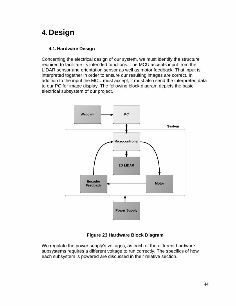
44

4. Design

4.1. Hardware Design Concerning the electrical design of our system, we must identify the structure required to facilitate its intended functions. The MCU accepts input from the LIDAR sensor and orientation sensor as well as motor feedback. That input is interpreted together in order to ensure our resulting images are correct. In addition to the input the MCU must accept, it must also send the interpreted data to our PC for image display. The following block diagram depicts the basic electrical subsystem of our project.

Figure 23 Hardware Block Diagram

We regulate the power supply’s voltages, as each of the different hardware subsystems requires a different voltage to run correctly. The specifics of how each subsystem is powered are discussed in their relative section.

45

4.1.1. Hokuyo UTM-30LX 2D Laser Range Finder The Hokuyo UTM-30LX 2D Laser Range Finder allows us to scan distances up to 30m away with high accuracy. This LIDAR can be controlled using USB connection with the provided SCIP ver2.0 protocol, which can handle up to 12Mbps of data. The laser operates between 10-12 volts. Since our system is designed on a 12V rail, there are no extra components needed to power this device. The UTM-30LX can scan up to a 270 degree arc with an angular resolution of .25 degrees, giving us up to 1080 distance values per scan. Using the SCIP interface, we can change the total scan angle, as well as the start and end points of such, as shown in the figure below.

Figure 24 Hokuyo UTM-30LX Scan Steps

(Figure used with permission)

Each scan follows the same series of steps, as seen in the figure above. Step 0 is the first measurement point at which the scanning unit is enabled, though no data is sent until it reaches step A, the initial measurement step of detection range. This step is very important, as it does not occur until the UTM-30LX has reached the desired starting angle provided by the user. Step B, the sensor front step, is reached at the same time each scan, as it is at a point normal to the front face of the device. Step C, End point of detection range, is the other user defined step. Similar to step B, this tells the LIDAR when to stop recording the data it is scanning. Steps B and C are very important, as they allow us to set our start and stop angles at any point outside of the dead zone. While the UTM-30LX has a maximum scan angle of 270 degrees between step A and step D, the LIDAR rotates through a 360 degree circle, such that it starts and ends at the same point each time. No matter the chosen scan angle, one full

46

rotation will always take 24ms. Once one full rotation is finished, the UTM-30LX sends out a 1ms low pulse. This 1ms low pulse is used for synchronous output. This allows us to not only be aware of a completed scan, but we can also use this synchronous pulse to drive the Dynamixel MX-28T Robot Actuator, coordinating the rotation between the two devices. The process of rotation and synchronization is shown in the figure below.

Figure 25 LIDAR Sync Pulse


4.1.2. Timing As microcontroller timing is critical for this project, we will needed to connect the synchronous output from the UTM-30LX to the Raspberry Pi. This is done by connecting the COM and synchronous output from the UTM-30LX’s 4-pin robot cable to two of the eight available GPIO ports on the Raspberry Pi. Each pin of the robot cable has a different purpose, but we only need to connect the Synchronous/Detection output and the COM output to the microcontroller for it to receive the 1ms Sync Pulse.

47

4.1.3. Power Requirements The Hokuyo UTM-30LX is designed to use a 12V DC power supply, though it is capable of functioning with a 10% tolerance, allowing a fluctuation from 10.8V to 13.2 V. While we plan to for the voltage to stay at a solid 12V to keep the LIDAR unit at a safe voltage, there is some room for leeway. The UTM-30LX typically draws 700mA of current during standard operation, but can pull up to 1A at maximum. The unit does not draw more than 8W total. If the UTM-30LX is not powered with over 10.8V the device does not function, though the low voltage LED is triggered to indicate that the in operation of the device is not due to a software or hardware error. If the UTM-30LX is given over 13.2V, it is possible permanent damage to occur in the hardware, a risk that must be avoided at all costs, as the LIDAR unit makes up a very large majority of our budget. The LIDAR unit will still display the green power supply LED if unable to draw the amperage needed, though its functions will be impaired. In this case, we can monitor the frequency of the sync pulses received to ensure that the unit is spinning at the correct 2400RPM. Similar to the previous case of excess voltage, if there is too much amperage in the system, it is possible for the system to receive irreversible damage to its main components. The UTM-30LX is designed to operate at a temperature range of -10° Celsius (14° F) to 50° Celsius (122° F). As testing and storage will occur in Orlando, Florida and the final product will be used in Virginia during in July, we need not worry about either of these temperatures. Orlando has never reached either extreme temperature, as its record low is 18 and record high is 103. Even in July, Virginia has never reached over 110 degrees thus will not conflict with the UTM-30LX. On the other hand, the LIDAR unit is also designed to operate at less than 85% relative humidity, which may be a possible issue given its Florida location. However, as the UTM-30LX has seen service in previous AUVSI RoboBoat competitions without fault, the device appears to be able to operate above its written tolerance, though the humidity of the lab will be monitored to avoid damage. The system will have an external DC power source of 12V and 24V. We will be utilizing the 12V power rail in order to supply most of the power to our devices. The 12V power source is supplied from a battery that is powering the external system. The external system is a mobile unit. It will be working in the field. This means that our laser range finder will be subject to environmental conditions that we must take into account when hooking up our power and data connections. Also, we will need to assume that the 12VDC that is supplied to our system is actually within operating range. With DC power systems, this cannot be guaranteed and usually the power will start high and drop lower as power drops. This means that our working DC voltage values are somewhere between 13.5V and 9V.

48

In order to compensate for this fluctuation of the voltage, we will need to look at each of our components. The Hokuyo 2D laser scanner can operate between the voltages of 10V - 13V. This is an acceptable range to deal with the fluctuation of the power. We will need to advertise our constraints to the external system to make the end user aware that the voltage will need to stay within that range. We monitor the voltage in our control system and provide a safe shutdown and a warning before the actual voltage drops below operating values and potentially causes damage or corruption within the system. The HD camera would be powered from the Raspberry Pi USB port. Since we are already regulating the voltage for the Raspberry Pi, it would provide regulated voltage to its daughter components. The logic pins on the Raspberry Pi will need to be corrected in order to be utilized. Most of the devices logic is in 5V, but the raspberry Pi logic is based on 3.3V. This creates the issue of overloading the logic circuits and potentially damaging the whole system. We will be using the 8-channel bi-directional logic level converter, TXB0108 in order to use the higher voltage logic on our lower voltage logic board.

Figure 26 Pinout of the TXB0108 8-Channel Logic Level Converter

(Reprinted under creative commons license)

4.1.4. Raspberry Pi Model B The Raspberry Pi model B allows us to use a credit card sized microcontroller to take and interpret in LIDAR data, control the Dynamixel MX-28T Robot Actuator and send interpreted data to the external display system. The raspberry Pi model B is powered by a 5v micro USB. The device’s current requirement is dependent the number of devices connected. We have found that purchasing a 1.2A power supply provides with ample power to run the Raspberry Pi. The model B commonly uses 700mA-1000mA depending on what peripherals are connected. The maximum power the Raspberry Pi can use is 1 Amp. The power

49

requirements of the Raspberry Pi increase as various interfaces are used. The GPIO pins can draw 50mA safely; (50mA distributed across all pins, each GPIO pin safely draw 16mA maximum), the HDMI port uses 50mA, the camera module requires 250mA, and a keyboards or mouse can take from 100mA to 1000mA. For our usage, the only things connected to the Raspberry pi during operation will be the Hokuyo UTM-30LX, the Dynamixel MX-28T motor serial connection, the pc, and the webcam. The Raspberry Pi model B microcontroller has a total of 26 available pins. These pins are used for different bus types, General Purpose Input/Output, as well as power and ground. The section below details the usage of each bus.

3.3V 1 2 5V

I2C1 SDA 3 4 5V

I2C1 SCL 5 6 GROUND

GPIO 4 7 8 UART TXD

GROUND 9 10 UART RXD

GPIO 17 11 12 GPIO 18

GPIO 27 13 14 GROUND

GPIO 22 15 16 GPIO 23

3.3V 17 18 GPIO 24

SPI0 MOSI 19 20 GROUND

SPI0 MISO 21 22 GPIO 25

SPI0 SCLK 23 24 SPI0 CE0 N

GROUND 25 26 SPI0 CE1 N

Table 7 Raspberry Pi Model B Pin Out A General Purpose Input/Output (GPIO) pin has a behavior defined by the user, and are unused by default. As such, each enabled pin can be either an input or an output; usage of the pin is at the discretion of the user. GPIO pins numbered 7,11,12,13,15,16,18 and 22. Also known as the Inter-Integrated Circuit Bus, the I2C is included to provide communications between multiple integrated circuits, including the Broadcom BCM2835 SoC processor built into the system. These pins also allow access to

50

the Raspberry Pi’s pull-up resistors, allowing for access to I2C functionality without needing external resistors. Specifically, pins 3 and 5 are for the I2C bus, pin 3 providing the Serial Data Line (SDA) signal and pin 5 providing the Serial Clock (SCL) signal. The I2C0 bus is not the only I2C available; however the I2C1 is terminated on the raspberry pi’s circuit board resistors and unavailable. The Universal Asynchronous Receiver/Transmitter (UART) bus is located on pins 8 and 10. Pin 8 is used for message transmission, pin 10 for message receiving. This bus provides a simple serial interface, requiring only 2 wires for access. These ports can be used to display kernel data if connected to a device capable of receiving and displaying the serial messages. While not necessary for any of our LIDAR functions, the UART bus is useful for debugging the raspberry pi if errors do occur. The Serial Peripheral Interface (SPI) Bus is used mainly for in-system programming, a process that allows an embedded device to be programmed when installed into a system, instead of pre-programmed. In our case, this would allow us to re-program the raspberry Pi on the fly. Unlike the previous I2C and UART busses, the SPI bus uses five pins instead of two, allowing for communication with more than one device. Of these five pins, pin 19 provides the SPI Master Output, Slave Input (SPI MOSI), pin 21 provides the SPI Master Input, Slave Output (SPI MISO) and pin 23 provides the Serial Clock (SCLK). The last two pins, 24 & 26 are used in tandem for Chip Select signals, allowing for up to two independent slave devices. The Raspberry Pi also provides two 3.3V and two 5V pins, along with four ground pins to complete any needed circuit. Unfortunately the LIDAR unit is unusable at such low voltage, as is the Dynamixel Servo.

4.1.5. Dynamixel MX-28T Robot Actuator The Dynamixel MX-28T Robot Actuator servo allows us to move the laser precisely. This servo can be controlled via serial communication and provides location feedback. This servo operates between 9 - 12 volts. Our system is designed around a 12V rail, so this servo will not have to have extra components in order to allow it to function. The servo rotation can provide us with 360° of motion. We will be utilizing all of this motion since the laser will be rotating in full circles to acquire the greatest amount of data. Since this servo will be in constant motion, it needs to have a tolerance for heat. The highest operating temperature of this servo is +80°C. Throughout our tests, we monitor the temperature and verified our assumptions that we will not exceed that temperature. The servo moves our laser and platform. The weight of these objects do not exceed the 2.6 Nm torque maximum of the servo. We did not witness any

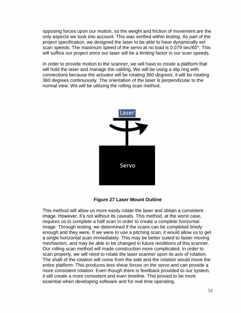
51

opposing forces upon our motion, so the weight and friction of movement are the only aspects we took into account. This was verified within testing. As part of the project specification, we designed the laser to be able to have dynamically set scan speeds. The maximum speed of the servo at no load is 0.079 sec/60°. This will suffice our project since our laser will be a limiting factor in our scan speeds. In order to provide motion to the scanner, we will have to create a platform that will hold the laser and manage the cabling. We will be using a slip ring with connections because the actuator will be rotating 360 degrees, it will be rotating 360 degrees continuously. The orientation of the laser is perpendicular to the normal view. We will be utilizing the rolling scan method.

Figure 27 Laser Mount Outline

This method will allow us more easily rotate the laser and obtain a consistent image. However, it’s not without its caveats. This method, at the worst case, requires us to complete a half scan in order to create a complete horizontal image. Through testing, we determined if the scans can be completed timely enough and they were. If we were to use a pitching scan, it would allow us to get a single horizontal scan immediately. This may be better suited to faster moving mechanism, and may be able to be changed in future renditions of this scanner. Our rolling scan method will made construction more complicated. In order to scan properly, we will need to rotate the laser scanner upon its axis of rotation. The shaft of the rotation will come from the side and the rotation would move the entire platform. This produces less shear forces on the servo and can provide a more consistent rotation. Even though there is feedback provided to our system, it will create a more consistent and even timeline. This proved to be more essential when developing software and for real time operating.

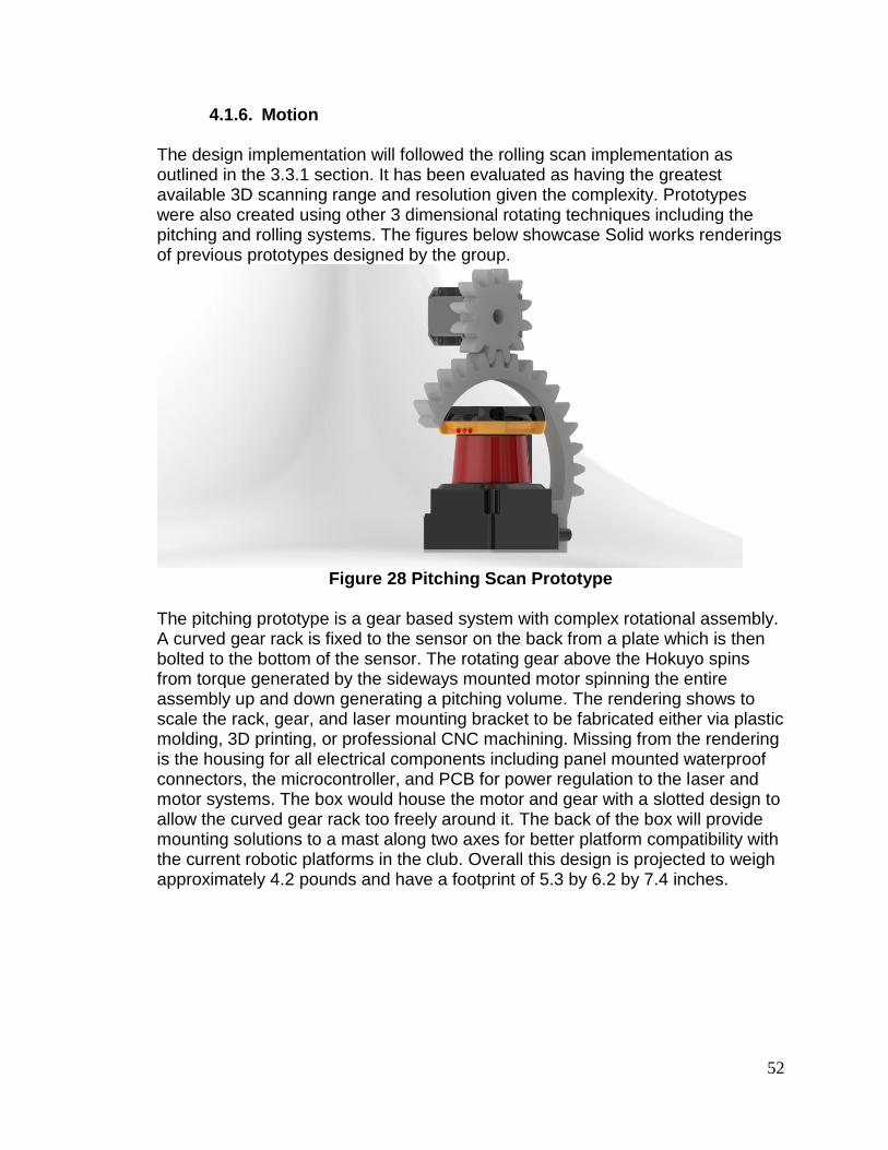
52

4.1.6. Motion The design implementation will followed the rolling scan implementation as outlined in the 3.3.1 section. It has been evaluated as having the greatest available 3D scanning range and resolution given the complexity. Prototypes were also created using other 3 dimensional rotating techniques including the pitching and rolling systems. The figures below showcase Solid works renderings of previous prototypes designed by the group.

Figure 28 Pitching Scan Prototype

The pitching prototype is a gear based system with complex rotational assembly. A curved gear rack is fixed to the sensor on the back from a plate which is then bolted to the bottom of the sensor. The rotating gear above the Hokuyo spins from torque generated by the sideways mounted motor spinning the entire assembly up and down generating a pitching volume. The rendering shows to scale the rack, gear, and laser mounting bracket to be fabricated either via plastic molding, 3D printing, or professional CNC machining. Missing from the rendering is the housing for all electrical components including panel mounted waterproof connectors, the microcontroller, and PCB for power regulation to the laser and motor systems. The box would house the motor and gear with a slotted design to allow the curved gear rack too freely around it. The back of the box will provide mounting solutions to a mast along two axes for better platform compatibility with the current robotic platforms in the club. Overall this design is projected to weigh approximately 4.2 pounds and have a footprint of 5.3 by 6.2 by 7.4 inches.

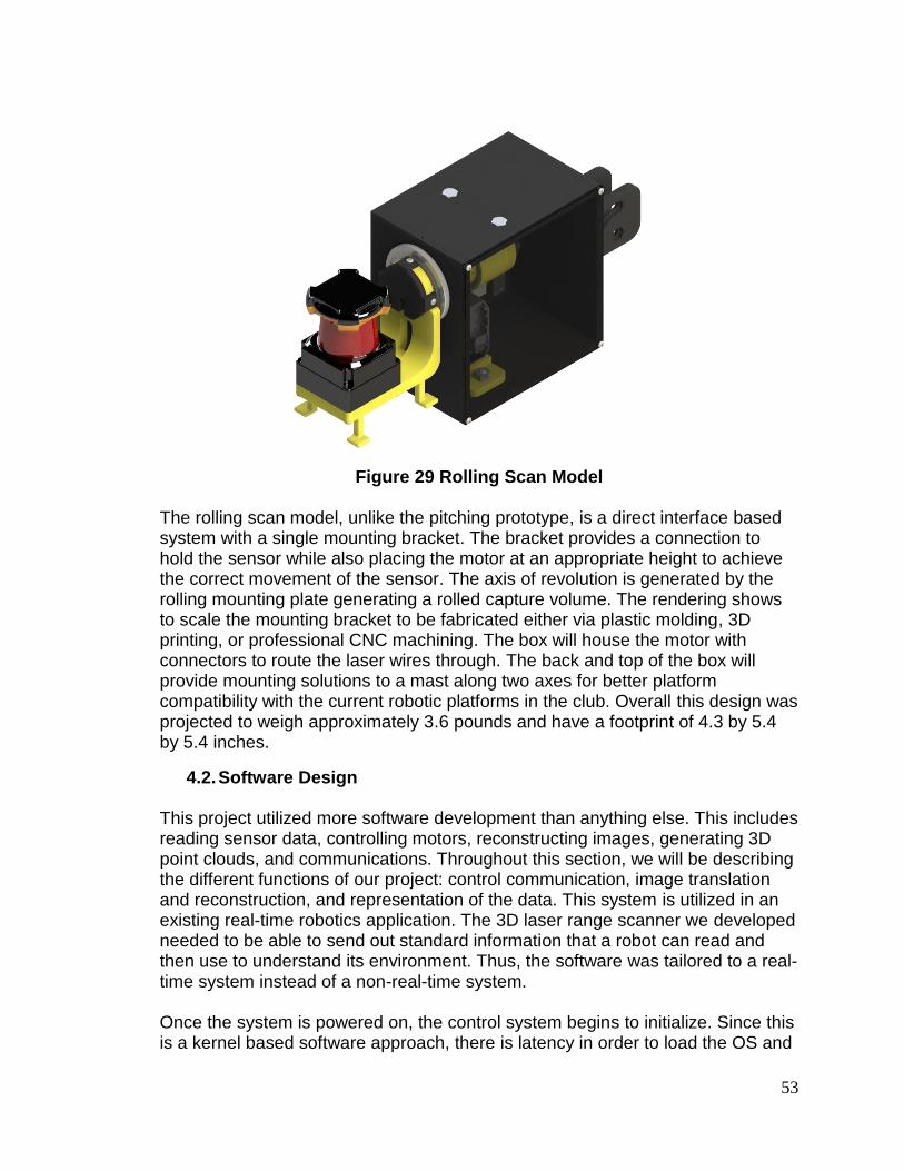
53

Figure 29 Rolling Scan Model

The rolling scan model, unlike the pitching prototype, is a direct interface based system with a single mounting bracket. The bracket provides a connection to hold the sensor while also placing the motor at an appropriate height to achieve the correct movement of the sensor. The axis of revolution is generated by the rolling mounting plate generating a rolled capture volume. The rendering shows to scale the mounting bracket to be fabricated either via plastic molding, 3D printing, or professional CNC machining. The box will house the motor with connectors to route the laser wires through. The back and top of the box will provide mounting solutions to a mast along two axes for better platform compatibility with the current robotic platforms in the club. Overall this design was projected to weigh approximately 3.6 pounds and have a footprint of 4.3 by 5.4 by 5.4 inches.

4.2. Software Design This project utilized more software development than anything else. This includes reading sensor data, controlling motors, reconstructing images, generating 3D point clouds, and communications. Throughout this section, we will be describing the different functions of our project: control communication, image translation and reconstruction, and representation of the data. This system is utilized in an existing real-time robotics application. The 3D laser range scanner we developed needed to be able to send out standard information that a robot can read and then use to understand its environment. Thus, the software was tailored to a real-time system instead of a non-real-time system. Once the system is powered on, the control system begins to initialize. Since this is a kernel based software approach, there is latency in order to load the OS and

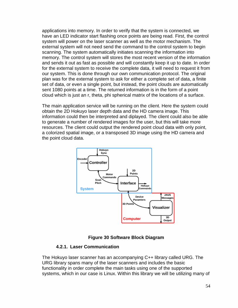
54

applications into memory. In order to verify that the system is connected, we have an LED indicator start flashing once points are being read. First, the control system will power on the laser scanner as well as the motor mechanism. The external system will not need send the command to the control system to begin scanning. The system automatically initiates scanning the information into memory. The control system will stores the most recent version of the information and sends it out as fast as possible and will constantly keep it up to date. In order for the external system to receive the complete data, it will need to request it from our system. This is done through our own communication protocol. The original plan was for the external system to ask for either a complete set of data, a finite set of data, or even a single point, but instead, the point clouds are automatically sent 1080 points at a time. The returned information is in the form of a point cloud which is just an r, theta, phi spherical matrix of the locations of a surface. The main application service will be running on the client. Here the system could obtain the 2D Hokuyo laser depth data and the HD camera image. This information could then be interpreted and diplayed. The client could also be able to generate a number of rendered images for the user, but this will take more resources. The client could output the rendered point cloud data with only point, a colorized spatial image, or a transposed 3D image using the HD camera and the point cloud data.

Figure 30 Software Block Diagram

4.2.1. Laser Communication The Hokuyo laser scanner has an accompanying C++ library called URG. The URG library spans many of the laser scanners and includes the basic functionality in order complete the main tasks using one of the supported systems, which in our case is Linux. Within this library we will be utilizing many of

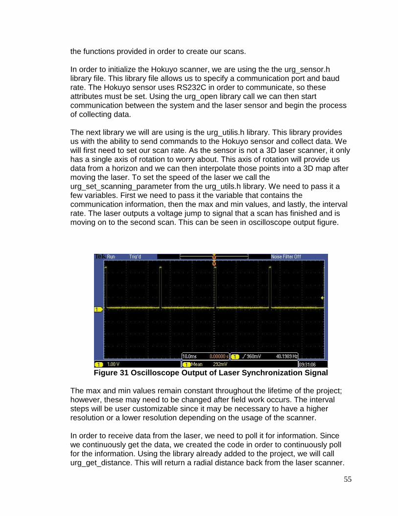
55

the functions provided in order to create our scans. In order to initialize the Hokuyo scanner, we are using the the urg_sensor.h library file. This library file allows us to specify a communication port and baud rate. The Hokuyo sensor uses RS232C in order to communicate, so these attributes must be set. Using the urg_open library call we can then start communication between the system and the laser sensor and begin the process of collecting data. The next library we will are using is the urg_utilis.h library. This library provides us with the ability to send commands to the Hokuyo sensor and collect data. We will first need to set our scan rate. As the sensor is not a 3D laser scanner, it only has a single axis of rotation to worry about. This axis of rotation will provide us data from a horizon and we can then interpolate those points into a 3D map after moving the laser. To set the speed of the laser we call the urg_set_scanning_parameter from the urg_utils.h library. We need to pass it a few variables. First we need to pass it the variable that contains the communication information, then the max and min values, and lastly, the interval rate. The laser outputs a voltage jump to signal that a scan has finished and is moving on to the second scan. This can be seen in oscilloscope output figure.

Figure 31 Oscilloscope Output of Laser Synchronization Signal

The max and min values remain constant throughout the lifetime of the project; however, these may need to be changed after field work occurs. The interval steps will be user customizable since it may be necessary to have a higher resolution or a lower resolution depending on the usage of the scanner. In order to receive data from the laser, we need to poll it for information. Since we continuously get the data, we created the code in order to continuously poll for the information. Using the library already added to the project, we will call urg_get_distance. This will return a radial distance back from the laser scanner.

56

We then pass it the device connection setup information and the input buffer value. The buffer will be allocated based on the desired range of view. Utilization of the C++ library will allow us to recreate a 2D map of a single scan. After which, we will use our developed application to translate those 2D maps into our 3D Point Cloud. There are numerous commands that we are using with the Hokuyo laser scanner in order to have complete operation. The following table provides the view of some of the members of the URGCtrl C++ library that we utilize:

4.2.2. Dynamixel MX-28T Servo Communication The Dynamixel MX-28T Robot Actuator will provide motion to the laser mechanism. This servo will provide the rotational motion on the x-axis of the laser scan. The servo is controlled using a serial connection from the microcontroller. It allows for setting of the angular position on the motor as well as provides feedback to the microcontroller. The servo will provide 0.088 degree accuracy which allows us to accurately reconstruct our 3D image. With this servo, you can initialize a starting point. This will allow us to run a calibration before starting our scans. This proved crucial in our code as we will need to make sure all values are correct and are relative to a given “zero” point. RS485 asynchronous serial is the method of communication for this servo. It allows for commands to be sent or received at any time. This is a type of two wire communication. It does not regulate or guarantee speed or accuracy in this serial communication standard. Compensation in the code was written in order to maintain a consistent line of communication. This servo allows for multiple baud rates. We chose a high baud rate In order to get the most real time information and also wanted to verify the amount of error from the line was minimal, which it was. Communication for the servo is done using an instruction packet. In order to read or write data, the memory address must be referenced. The two section of memory are the EEPROM and RAM. The EEPROM can be used to program values of the servo that will not be erased power is removed. Alternatively, RAM is only used to operating values and will not remain in memory without power.

4.2.3. Webcam Communication Communication to the HD camera could have been achieved through a custom library that runs in the user space of the Linux operating system called VideoforLinux2. This is software accelerated so the image will need to be buffered and then rendered for each image. We would have been able to control the access that camera has and may only need to take images every few seconds or we may sample from a video feed.

57

4.2.4. Platform Communication The goals of this project it was to be able to create 3D spatial representation of an environment for use on a kinetic robotics application. We needed to output to the robot a dataset representative of what is in front of it. We will be utilizing a serial connection for data extraction from our system. UDP communication allows us to communicate the point cloud information with any listening clients. This will allow us to create a packet that contains the necessary information. The robot will interface with our LIDAR system and output the point cloud information. We will create a set of predefined commands that will then get an appropriate response. Most of the time it will be requests for location data, however there are additional functions that allow settings to be altered such as sampling rate, sampling angle, maximum and minimum degrees for the field of vision, and other various settings. The packet structure used will contain a header file that provides basic information for transmission of the data. It will contain at least the initialization bit for the transfer, the packet length and a format ID. The packet will then contain the payload. This payload depends on the context of the situation. If the system was asked to supply information about the orientation of the laser scanner, then the payload will contain a specially created payload for representing that data. We had hoped to create a protocol similar or compatible with the ASPRS LIDAR Data Exchange format. This is a standard used by existing LIDAR systems; however there are numerous points of that protocol that do not apply to our project. For instance, we do not have a GPS on our system and one of the requirements on this standard is that we have GPS coordinates. We chose not to include this standard. The coordinates will be output constantly and will be supplied using the most recent scans. The system is not designed to remember or map out the 3D environment, but only to show what is currently known and can be seen for use for awareness and avoidance. The packet can come in multiple ways depending on the request. Originally, we allowed the request for a complete image and then we will supply a full 3D point cloud of the current image, but was altered after testing proved that it took too long to transfer that data. The method we used returns of only a portion of our known image, it returns a single scan from the 2D Lidar with interpolated r, theta, and phi points. This was useful for applications as the data needed to be smaller in order to transfer in real time over UDP. At this point the client can manipulate the point clouds as it sees fit. It may be useful if only a certain section is being monitored and waiting for movement in order to react. The other method that data can be viewed is scan by scan. The client could only to see the newest scans that it has received. There may be a wall in front of the laser scanner that exists and when the wall is removed, the application may want to react, but this is up to the client.

58

Each type of packet request data was going to have an identifying ID associated with it that is known in the protocol we would have developed. These numbers could have been any arbitrary ID, but it would have to be unique. In order to have a unique ID, we will be using 3 Bytes of data. This would provide us with a sufficient amount of data to have many commands as well as having the ability to discriminate which commands were sent. Each of these commands will then have a known structure. The payload may be larger or smaller depending on the command and will each contain a byte for length at this level if the amount is dynamic. Otherwise, it will be a known static length. Each of the payloads would have a known termination byte sequence established with the protocol. This is will serve as the flag that the data is complete. Once the header and payload have been finalized, the whole packet will need a checksum or sorts. A CRC could be calculated on the packet and tagged on to the end. This CRC could then be calculated on the receiving end to verify that the data packet they have received is complete. What was actually used was a UDP multicast transfer. Once the Lidar was operational, it begins sending out packets that are compiled and adjusted. It sends one 2D lidar scan at a time until the queue is empty. At the same time, more scans are added to the queue. This limited the amount of data sent out at once and allowed for real time rending on the client side. We found that this method utilizes about one megabyte per second of network bandwidth. Since it is multicast, anyone on the network can listen without hindering the Pidar.

4.2.5. 3D Creation To fulfill the goals of this project, a 3 dimensional image had to be created. The 3 dimensions will be the r, theta and phi or depth, angle to depth, and angle of motor respectively. In order to create the image, we must first read the sensor data of the Hokuyo 2D laser. This information will only provide us with the horizontal and depth portions of the image. This information will be obtained and retained in memory. Depending on the scan resolution decided by the configuration of the user, the system will tilt a certain number of degrees to obtain a second 2D scan. This again will retain into memory. This pattern will continue continuously and a full image is obtained when the motor has rotated 180 degrees. It then continues to rotate to get an additional image. Depending on the speed of the scans set in the configuration by the users, a single scan should not take much time. The time to scan should be set sufficiently to provide an accurate representation of the image ahead of it before that image can change. Now that the memory is filled with N numbers of 2D scan lines the process of placing them together can occur. Depending on the ability of the code, this may happen in tandem with the scanning. The 2D scan lines are based on radial distances. These distances must be corrected for timing between the laser and the motor. We will not discard this information, but are merely interpreting it. These polar coordinates may be beneficial to the attached system as they will

59

attribute angle as well as magnitude of a certain object. We will repeat this process for all of the scan lines that were taken. The 2 rotational components are the laser scanner which is rotating on the y axis and the platform that is rotating along the x axis. The polar lengths will correspond to both of those rotations. This will mean that we will be taking the magnitude of those points and projecting it onto our new image.

Figure 32 Projecting 2D Image from Radial Scan

With our image we will retain a map. This map will allow us to maintain the information of the distances at each of the points; this is called a point cloud. With this information we can represent the image in corrected 3D. This will allow for a screen representation and rendering. This also will allow for finer adjustment and debugging. In order to achieve this transformation we will need to utilize a formula for projecting an image onto a 2D surface. The following formula will allow us achieve this action:

This formula represents the projection of an image through a camera matrix. The

camera represents our point of view. The represents the amount of rotation and translation from the original point that is used when transforming to the 2D image. Applying this formula will be done using existing libraries within the OpenCV library. It is determined by the client which angles are appropriate for viewing.

4.2.6. Point Cloud Previously, we have described how to scan in the 2D images and create an image. The distances that correspond with those points allow us to create a map in 3D. This is called a point cloud as seen in figure 37. Using the 2D information that we have collected we can create a 3 dimensional array of information.

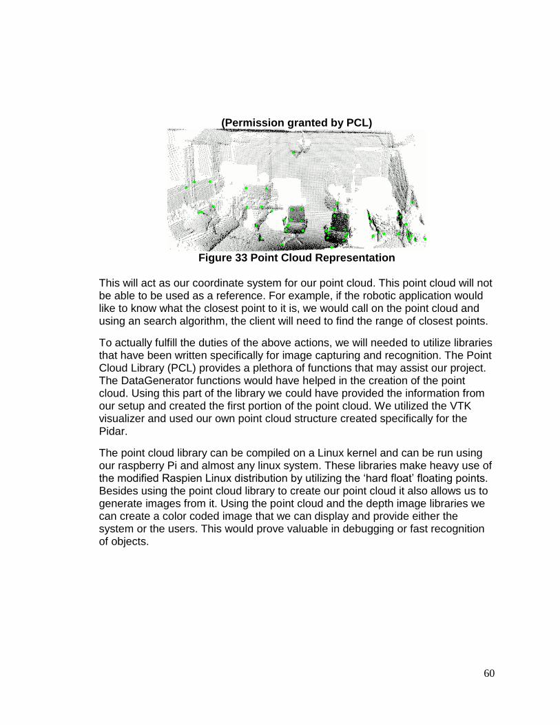
60


Figure 33 Point Cloud Representation

This will act as our coordinate system for our point cloud. This point cloud will not be able to be used as a reference. For example, if the robotic application would like to know what the closest point to it is, we would call on the point cloud and using an search algorithm, the client will need to find the range of closest points.

To actually fulfill the duties of the above actions, we will needed to utilize libraries that have been written specifically for image capturing and recognition. The Point Cloud Library (PCL) provides a plethora of functions that may assist our project. The DataGenerator functions would have helped in the creation of the point cloud. Using this part of the library we could have provided the information from our setup and created the first portion of the point cloud. We utilized the VTK visualizer and used our own point cloud structure created specifically for the Pidar.

The point cloud library can be compiled on a Linux kernel and can be run using our raspberry Pi and almost any linux system. These libraries make heavy use of the modified Raspien Linux distribution by utilizing the ‘hard float’ floating points. Besides using the point cloud library to create our point cloud it also allows us to generate images from it. Using the point cloud and the depth image libraries we can create a color coded image that we can display and provide either the system or the users. This would prove valuable in debugging or fast recognition of objects.

61


Figure 34 Range Image

4.2.7. Real World Image In order to produce a more human viewable image we would have liked to be use an HD camera. This camera would have taken images of the scene in front of it. The camera would not always be sending the data, we would have to request that an image be taken sometime during the course of the scan. Once we had buffered the image we would have used an algorithm that correlates the captured image to the coordinate in our point cloud. Since we know the physical dimensions of the capture mechanisms and we know that images between them will have a consistent differential, we could have used a static approach to mapping the image. Other methods may have required us to use special image recognition techniques. However, we will still need to apply those techniques to produce a better looking image, but would not be the foundation of our alignment. In order to approach this problem, we could have used the open source computer vision library ‘OpenCV’. The OpenCV library contains methods that allow for translation of imagery to point cloud data. Before the OpenCV libraries can be utilized, we must remember that the point cloud data must be created to comply with both the point cloud library (PCL) and the OpenCV library. To get the most accurate settings, we will first estimate the angles and dimensions based on the physical construction. However, this estimation will be improved over time through testing and aligning. This testing and aligning will take into account all of the intrinsic properties of the camera setups that we may not be able to accurately measure or take into account. The resulting image would be a roughly 3D modeled image that should resemble the actual world in front of the cameras. This output is intended for a human viewer, as a robotics application may not have use for the real world image. However, this will be included as part of our output communication possibilities because there may be an application that may use the real world image. For instance, some applications may use this to provide object identification and retrieval based on color and shape. The HD camera will allow the application to view color as well as its physical makeup.

62

4.2.8. Dynamic Configuration Our application allows for the ability to manipulate settings. Based on our observations, we hard coded in the default settings into our application. However, the unit will be completely customizable using our outward facing interface. The settings will include the ability to customize the laser sensor resolution and speed, the motor angle and speed as well as image formatting. The laser settings will not be directly accessible for the end user. Because there will be some custom formulas and libraries involved, we cannot allow the user to directly alter the laser information. However, we will provide a function that will enable them to do such. When the user desires that a laser scanner be slower or faster or specifies a resolution, we will then insure that all appropriate settings will match. All of the calculations will need to be altered and the images will have to be adjusted in order to compensate for lower or higher resolutions. If the speed of the laser scan is adjusted, then we may need to compensate on our motor in order to allow a complete scan to complete. The motor settings are similar to the laser settings in that we do not allow for direct access. The motor control functions can be accessed using a custom function call to our system and will guarantee that all appropriate settings are altered, just like when the laser settings were altered. With the motor, we will also need to put constraints. We will have to have a maximum and minimum value for speed and angles. We also have to check each setting that the user chooses to check for problems during runtime. Now that we developed the final 3D laser range finder, we can create curves that can be supplied to operators to know the proper operating constraints. The communication system provides the ability to talk to our 3D laser range finder. We will have a default and persistent method of communication via an Ethernet connection that will always be able to listen and set settings. This could be considered our ‘direct access’ method. Using this, users or applications could communicate to the rangefinder to turn on or off settings and alternative communication means. A secondary communication system could be developed that will communicate through a website. This would allow the user to see and set configuration information in a more convenient and quick manner. This setting would have been optional and could be turned on and off depending on the user preferences. The output display for the user is provided by obtaining multiple single scans and buffering them to create a complete image. Based on the speed of the scans, it may take less than a second to create a complete scan. This reduces the load on the system by just getting the raw data instead of having the render take up processing time and power on the raspberry Pi. The data can be viewed in a number of different ways. The user can view just the point cloud information and will see only dots that form the 3D environment. The user can view a color coded

63

range image that provides a depth map represented in 2 dimensions. The user could also have viewed an overlay image where the 2D image is transposed onto the 3D point cloud if it was developed. Finally, the HD camera 2D image could also have be requested. This image would not have any manipulation, but would allow the user to see what is seen without any form of translation. All of these settings will be configurable on the 3D laser range finder.

4.2.9. User Interfaces There is not a single interface for the 3D laser range finder. Since a communication protocol is being developed, this has the possibility to have an interface developed for just about any platform. For development, as well as other Linux platforms, we will be creating a basic graphical interface. This will supply us with an ability to see all of our available settings, change settings, view images, render images, and export data.

Figure 35 Graphical User Interface Mockup

In order to create the graphical application we will first created a command line application. This command line application was able to process our commands using a known set of instructions. These instructions will correlate to the different classes we are developing. We choose to use a command line version of the application because it will simplify debugging process since we will not have to debug between the window representation and the actual program processing the image data.

64

Once the command line version of the application is completed, we created the graphical interface. Qt is a multiplatform framework that provides simple window management. The following bulleted lists display the current officially supported operating systems. Desktop Platforms

Windows Linux/X11 Mac OS X

Embedded platforms Embedded Linux (DirectFB, EGLFS, KMS, and Wayland) Windows Embedded (Compact and Standard) Real-Time Operating Systems, such as QNX, VxWorks and INTEGRITY

Mobile platforms Android iOS Windows 8 (WinRT) BlackBerry 10

All, or portions, of our application can be ported to any of the listed supported platforms. The work load may need to be offset onto the original hardware so calculations can be processed locally when the client hardware may be lacking the processing power or support that may be required. Qt uses C++, which is useful since our libraries and application will all be written in C++ as well. While developing the code for our Qt application we were using a Qt supplied Qt creator for C++. The Qt creator is custom tailored for developing Qt applications; unlike eclipse which utilizes a plugin to allow for creation and modification of Qt C++ applications. Using Qt we can create a C++ library of our application instead of using the command line version. We will have needed to develop the command line version anyway first to test, but this allowed for a more streamlined graphical version of the application.

4.2.10. Network Access Our 3D laser range finder communicated via a network. Onboard of the raspberry Pi is an RJ45 connection. This connection can be utilized by network traffic to provide a basic network access. This is the valuable to the project as it is the only method to obtain the point cloud data. Although, it is not in our currently design, a website could have served as a testing mechanism or feedback mechanism when our range finder is not attached to another system. A basic website could be provided that displays the information from the range finder. By default the most basic of information would be available on a plain website. We will provide the source and instructions to any users of our range finder in order to customize

65

the output. The web service would need to be hosted locally by an onboard web host called apache. This could provide multiple socket connections to the board and return values that have been made available to it. The reason this onboard system is so light and low priority it serves little purpose for actual production usage, but may assist in development, alignment, or setups. An option for end users of the 3D laser range finder may be that they create their own website to interact with it. Since the information will be available to their existing system, they may have wanted to send that data back to a home base and from there supply a website, app, twitter feed, etc… with information. This way the end user can relocate the resources off of the main system so it can work more effectively. The hosting software would most likely be running a PHP server. PHP would allow us to interact with our system dynamically without having to recreate the entire code for the site. In order for the PHP system to work, we would need to implement a sort of swap file for our data that is accessible to both the Apache server and our main control application. Common swaps file for use in a MySQL database. These databases could allow for multiple applications to connect, access, and modify data at the same time. This would give us the most up to date information in order to output to the server.

4.2.11. Output Protocol The most important part of our system is the output information. In the case of our 3D laser range finder, we had hoped to have multiple ways to access the data. Originally, we would make our data accessible to other systems using a custom TCP protocol, however, it was abandoned after testing. In order to communicate, we would have first needed to establish a serial connection. The connection would have a default port and baud rate that can be customized in the main application. The main application would listen for a client request indefinitely. Once a connection is established, then the system will be able to take instruction and output data. We will have different types of data, each of which will have corresponding codes. These codes will be established within our communication protocol. Our protocol will be able to be encapsulated within another form of communication such as RS232 or TCP, so long as our final result allows us to send and receive data to and from our system in a quick and accurate form. Within our original communication protocol we wanted to establish a form of error check. This error checking will consist of creating a cyclic redundancy check (CRC) code based on the contents of the packet. This CRC code will be accessible, but not required. We would have allowed for the option to ignore the CRC code in the options. Some applications may want to have the CRC code to insure they receive perfect data each time as well as a complete set of data. In order for CRC checking to occur, both sides of the communication would have to

66

have the CRC hash table. This would have needed to be an agreed upon hash table, which the default will be provided by us, but some applications may wish to alter this table to allow for larger data sets or faster calculations. Overall, the communication protocol will be similar to that of existing protocols such as the transmission control protocol (TCP) or the user datagram protocol (UDP) in the sense that they will have a complete reconstruction of data or allow for data loss. That decision would have depended on the user and depend on the option or action that is selected. Our original protocol would have included a header file that contains information about the data packet. It will start with a packet declaration. This is a known bit sequence that will tell the receiving end that a packet is starting. The length of this sequence would be decided upon after testing, however, we would have chosen to start with a 4 bit sequence to begin with and move up from there if we encounter false starts. If we chose to go any lower, we may get many false patterns of the same sequence and will falsely tell the receiving end that a new packet has started. After the header we will have the total length of the packet. This will allow the receiving end to retrieve the packet out of the buffer and begin its decoding. After the initialization code and the length, there would have been a 3 Byte action code. Having a large action code will provide us with more than enough unique action calls and will leave plenty of room for more. These calls are for specific requests that correspond to a known action. For instance the code AAA [hex] may correspond to the reset command. The receiving end will see 1010 1010 1010 [binary] come in the action command portion and know that the system will need to be reset. This sort of command will not have any more than this information, so there would be no need to have any additional information. However, for complex commands, a form of subcommand may be necessary.

Packet Section # Bytes

Initialization Byte Sequence 4

Length 2

Action Code 3

Packet Data 16

Sub-Packet Data

CRC 1

Table 8 Packet Layout Some commands would require more complexity than a 1 step command. To be able to accommodate for these commands there would have to have a tiered structure. The action command will in turn have another sub-action command. This structure could potentially continue until we reach the limit of the maximum packet size. For example, if the action command for moving the laser scanner was requested, then how would it know where to move it? How fast? This action

67

command for the laser movement will be received, but then a second action command will follow stating which direction. After this the packet will contain the information that states the information of where to go and how fast. This structure for decision making will allow us to create in depth, accurate and useful commands that are accessible to the connected system. Another major benefit of creating a tiered custom protocol is that the system can be thought of to be object oriented. The information is in container form and can be represented in an easy to read, easy to understand, easy to implement manner. Also, due to the ability to have dynamically sized commands and new commands, the host system can be updated with new commands and action and protocols without breaking the client. The client could be updated to allow for new commands or to continue to utilize the old commands just as it would have in the past. There are many types of commands that we would have to handle. There was the query and response commands that will be short and finite. These include items reported values or canned responses such as a ‘Ready’ command or a version number request. These commands let the attached system communicate with the 3D laser range finder and obtain information about its setup values. This would allow the connected system make decisions based on those values and possibly update the values if need be. This brings up the next type of commands, which are settings. Setting commands would provide a valid value to be set inside of the program. Given the nature of our protocol, we can do error checking on the host side before actually using these values to insure that they are valid. Once a setting is set or denied a response is sent back of either OK or ERROR.

68

[Base16]

A01 Initialize System Requests that a connection be established A02 Start System Tell the system to start scanning and

generating data A12 GetReadyStatus Query Requests a confirmation that the system is

ready. Returns OK, KO, or nothing A13 GetVersionInfo Query Returns the version of the protocol A14 GetCurrentPosition Query Returns the current angular position of the

3D scanning mechanism A15 GetLaserSpeed Query Returns the current speed setting of the laser A16 GetMotorSpeed Query Returns the current speed setting of the

motor A17 GetCameraRefresh Query Returns the refresh rate of the camera A18 GetErrorCodes Query Returns any pending error codes B15 SetLaserSpeed Setting Set value of laser speed B16 SetMotorSpeed Setting Set value of motor speed B01 SetMinimumScan

Angle Setting Sets the minimum scan angle from 0 - 180

degrees B02 SetMaximumScan

Angle Setting Sets the maximum scan angle from 0 - 180

degrees. CD1 GetDepthFrom

Coordinate Image Returns the best value of depth based on the

provided single coordinate CD2 GetDepthFrom

CoordinateRange Image Returns the depth values of a given range of

coordinates CD3 GetDepthImage Image Return the entire depth image matrix CD4 GetDepthColorized

Image Image Return the depth image rendered with color

to designate distances CC1 GetCameraPixelData Image Returns the value at a given coordinate from

the camera CC2 GetCameraRange

Data Image Returns the values of a given range from the

camera CC3 GetCameraImage Image Returns the entire camera image A0A EmergencySTOP System Emergency Stop. Stop moving. A1A Stop System Stop gracefully AAA Reset System Reset software and positions

Table 9 Original Laser Range FInder Protocol Codes Our initial protocol also included constructive error responses. When our system receives a bad command, it will try and return the error code and/or message with it. For instance, if the command ‘move laser left 200 degrees’, we will return an error because the laser can only go 0-180 degrees. Depending on the settings, the system may move to the furthest constraint of 180 degrees, but still return an error because it could not complete the full turn. The error packet will include an error type code, the original command code and a constructive ASCII message. The ASCII message is in plain text. This would be so the attached system can include a human readable error message that can be used to troubleshoot.

69

Error Code Meaning

F00 Invalid Command

F02 Incomplete Command

F04 Value Out of Bounds

F08 Bad CRC

F16 Duplicate Request

FAA System Not Ready

FAB Hardware Unresponsive

FAC Timeout

Table 10 Error Codes

4.2.12. Command Sequence The scanner will function by providing feedback to the external system that information has been received and executed successfully or not. This allows the external system to have an absolute understanding of what is currently being performed on the scanner. This procedure can be seen in the figure below that demonstrates how the system should have operated with these commands and errors.

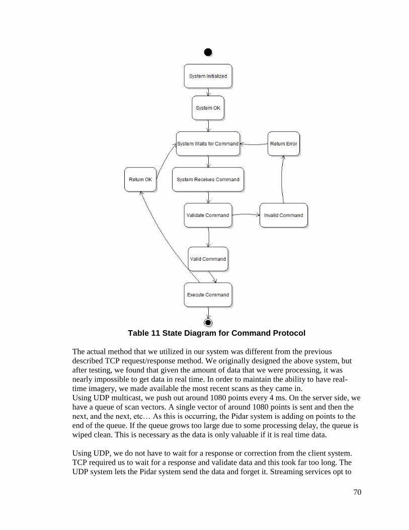
70

Table 11 State Diagram for Command Protocol

The actual method that we utilized in our system was different from the previous

described TCP request/response method. We originally designed the above system, but

after testing, we found that given the amount of data that we were processing, it was

nearly impossible to get data in real time. In order to maintain the ability to have real-

time imagery, we made available the most recent scans as they came in.

Using UDP multicast, we push out around 1080 points every 4 ms. On the server side, we

have a queue of scan vectors. A single vector of around 1080 points is sent and then the

next, and the next, etc… As this is occurring, the Pidar system is adding on points to the

end of the queue. If the queue grows too large due to some processing delay, the queue is

wiped clean. This is necessary as the data is only valuable if it is real time data.

Using UDP, we do not have to wait for a response or correction from the client system.

TCP required us to wait for a response and validate data and this took far too long. The

UDP system lets the Pidar system send the data and forget it. Streaming services opt to

71

use UDP packet data since it allows for realtime applications that loss is fine. If we lose a

few points in a million, it will not severely harm the client system. The other benefit is

that using multicast, any client on the network can obtain the points. This can allow for a

robot to analyze the data at the same time as the user and they can debug more easily.

The command structure to setting points is done using UDP as well, but is done via

ASCII. A command such as “CS10” changes the speed to 10 rpm. The server will then

respond by saying “OK”. Again, UDP is best effort and is not guaranteed, so it is up to

the client to verify that it has occurred.

4.2.13. Output There would be different types of images and data that would be able to come out of our system. Requests by the attached system would have mandated which types of images are create and reported back. Although we would like to have provided the ability to render images on the system, it is not recommended due to the limited resources available. The optimal situation was to use a 3D rendering software to render our raw point cloud data. This allows the user to rotate an image and have the ability to change the view perspective. If we render the image on the system it will be static and from only our default viewing angle. The Qt software we are developing will be able to run under Linux and be able to interpret our output data to display a few basic images. Since we will be developing a custom API to connect to our system, anybody will be able to access the data that has access to the device. Custom software could be written that calls and utilizes data differently. The 3rd party software Mesh Lab can be utilized to display our point cloud data information after it is saved from our custom client. The static rendered images that we will be producing will utilize the Point Cloud Library and OpenCV. Between these two libraries, we would be able to identify key points in the images; correct the images to display properly, render the images using key points, and output the data. The types of images we create can be very detailed or very shallow. We can also filter out pieces of images that are too far to matter. If the external system does not want to see anything beyond 3 meters, then the system can make anything past that point null and only show the pieces of objects that are within the distance threshold. Although these images will be close to what we want, they are not our complete images. In order to display the entire image, we will need to render the full 360 degrees. The system can be set up to only utilize a certain range of angles, which would automatically be used for rendering. In order to display 3D data within a 2D field, we will colorize the image based on color key to represent depth. Using a custom written function, we are able to colorize the image based on distance from the Pidar. Other images we can create are point images. This will merely map the points of the data in 3D space from a specific perspective. The size of the dots will change based on the

72

distance away from the camera. This will provide a basic view of the key points that make up the depth imagery. This type of image is less resource intensive to produce since it is using just the coordinates from the point cloud data to create the image. Another image we would have liked to produce would have been a 3D mapped image that has an HD camera image overlay. This would be the most intensive image to render as it will require the use of the OpenCV library as well as the point cloud library. It will need to look for key points, skew the image appropriately based on calculable data, and shift images based on depth. The view of this image will not be able to be used from the center perspective as everything will look 2 dimensional. This means that the perspective viewing angle will need to be shifted off center. The benefit of our method for outputting data is that it is much more scalable and dynamic than a single output device. The network protocol will allow for use from different external systems. The API can be scaled and upgraded without damaging existing setups. The output imagery is useful to the users that are using this device as they will be able to see and understand what is being fed to their system. The output imagery can also be upgraded. If we develop a new rendering method, we can then upgrade the software and be able to provide those images additionally. The overall ability to be able to update, modify, and completely customize our sensor will make it viable for almost all relevant applications.

4.2.14. Linux This project is using Raspien for the Raspberry Pi ARM microcontroller. This is a deviation from the Debian Linux distribution that is specifically tailored for the Raspberry Pi. This port provides an improved “hard float” calculation that allows it to utilize the floating point hardware calculation of the ARM processor. We will be able to use a graphical environment and therefore interact and monitor our software while we are developing and debugging. To alleviate some resources, we chose to remove the added window manager to solely provide a console based environment. The Linux environment serves a great purpose for us. It allows us to utilizing multitasking. In order to scan data, interpret data, and output data, we have to multitask. This is all done on the ARM processor and is completed using threaded applications. We are prioritizing our processes as well to ensure that the most important processes get the CPU first. The highest priority application will be the laser scanning software. This must always remain fresh data or else it will completely undermine the whole project. If the project were to give priority elsewhere, than our LIDAR system may in fact feed incorrect information. This is unacceptable because the output of this system will be treated as true every time. So that is why the scanner portion has highest priority.

73

4.2.15. Raspien OpenCV Package The OpenCV library can compile for Raspien and provide the image translation functions. However, we did not end up using any image manipulation libraries on the raspberry Pi. We would have written the code that utilizes OpenCV as well as the interpretation software to generate the 3D point clouds. OpenCV would serve to allow for image homography alignment for our webcam image and our 3D point cloud. This will be for display. Inherently, this would have provided a 2D image that can then be used for other calculations or for demonstration data. We would be using the image processing, or imgproc, portion of the OpenCV library to fit the image from our webcam to a round image. The Structural Analysis and Shape Descriptors portion of the library will allow us to perform these tasks using algorithms that have been developed, testing and run numerous times by many people. This would leave us with the task of collecting the data necessary in order to provide the correct input. The Camera Calibration and 3D Reconstruction portion of the OpenCV library would have been used once we have our complete x, y, z scan. We would use the function such as findHomography in order to correctly map our image. The function calibrateCamera will be used during our development, but will not be required during the running process. However, if the camera were to have changed, then the code would need to be recompiled using the corrected values. ReprojectImageto3D would have assisted us in rendering the final images that will be human readable. This will allow for debugging and for fast understanding and representation of what is being seen by the LIDAR.

4.2.16. Programming Languages C++ was the language of choice for our application. This was chosen because the most difficult communication we will encounter is the laser scanner and the library provided is in C++. Additionally, the ability to allocate and clear memory when we need it is crucial to our program as we need it to be as efficient as possible. Other languages such as Java do not allow for this level of memory efficiency. We are utilizing the latest stable version of GCC, a C++ compiler. Project setup will utilize the cross-platform open-source build system known as QMake. Essentially Qmake tools allows for developers to create projects which are platform, and usually operating system, agnostic. The novel idea can allow for programs and projects written on closed source IDEs and systems such as Windows to be setup in a way which when distributed can instantly be built, compiled, and linked using any other operating system or IDE (theoretically). The build scripts written using QMake are output from the Qtcreator software automatically. This powerful tool enables developers who switch between different systems frequently the power to move those desired applications with them. Many of the libraries and software packages used and mentioned, like

74

OpenCV and PCL, all leverage the QMake build system. This widely used build system will enable the LIDAR system proposed to be cross-platform as originally intended and required by the given software specifications. QMake can enable greatly enhance the efficiencies and logistics required in teamed programming applications since it does not require any given computer to have specific software or virtual machines for the applications to compile.

4.2.17. IDE The programming environment that we utilized on the Raspberry Pi will be qt creator. This will allow us to have a simple GUI based method of interacting with our program. For the majority of the code, it will was written elsewhere and then placed into our project on the Raspberry Pi. Debugging was done using the Raspberry Pi since we will be heavily dependent on memory, pins, libraries, and COM ports. This gave us the freedom to use any regular IDE such as eclipse or QT for C++. Maintaining our code was performed using a GIT system. This allowed each of us to develop code and then merge that code into our main source. It provides us methods of reversing if we need to. This also provides a cloud-based backup system of our code in the event that a hard drive has become corrupt. Using GIT we each need to have a uniquely identifying login. This will allow us to have individual branches that we can each work on and can merge when necessary. IDEs such as eclipse have but in GIT source control plugins that we utilized that made the task easier and more streamlined.

75

5. Executive Design Summary

5.1. 2D Laser Specifications The figure below shows the Hokuyo UTM-30LX 2D LIDAR dimensions and footprint. This schematic was referenced heavily as prototyping of the 3D assembly continues into the subsequent semester. This laser has two cables providing data and hardware synchronization. It has a footprint of 60 by 60 by 87 mm and weighs approximately 370 grams.

Figure 36 Hokuyo 2D Dimensions

(Reprinted with Permission)

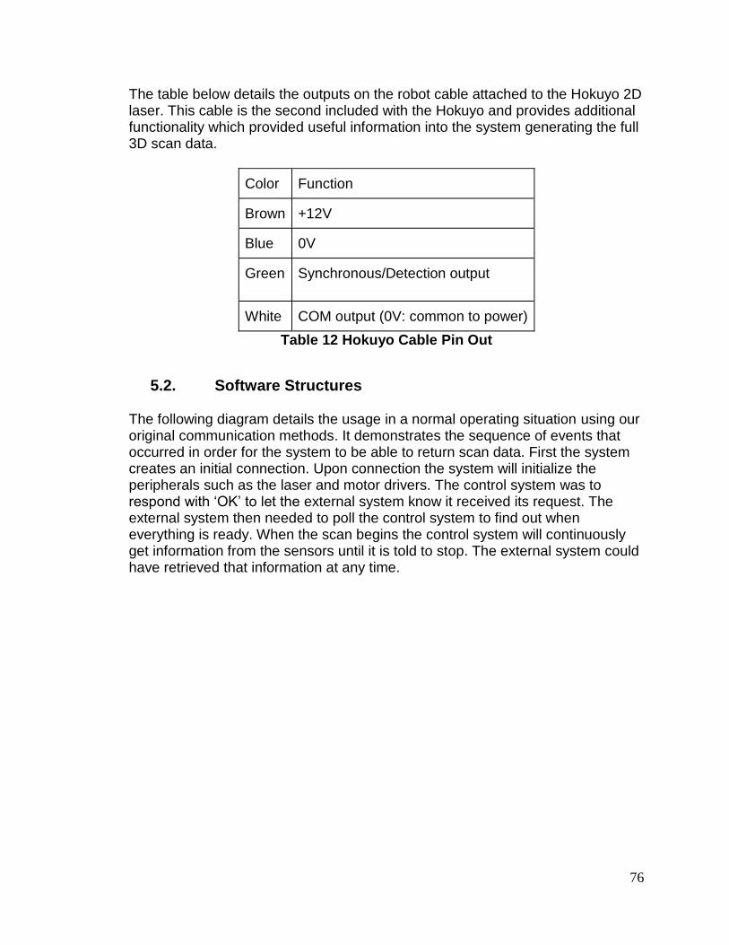
76

The table below details the outputs on the robot cable attached to the Hokuyo 2D laser. This cable is the second included with the Hokuyo and provides additional functionality which provided useful information into the system generating the full 3D scan data.

Color Function

Brown +12V

Blue 0V

Green Synchronous/Detection output

White COM output (0V: common to power)

Table 12 Hokuyo Cable Pin Out

5.2. Software Structures The following diagram details the usage in a normal operating situation using our original communication methods. It demonstrates the sequence of events that occurred in order for the system to be able to return scan data. First the system creates an initial connection. Upon connection the system will initialize the peripherals such as the laser and motor drivers. The control system was to respond with ‘OK’ to let the external system know it received its request. The external system then needed to poll the control system to find out when everything is ready. When the scan begins the control system will continuously get information from the sensors until it is told to stop. The external system could have retrieved that information at any time.

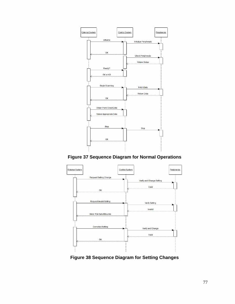
77

Figure 37 Sequence Diagram for Normal Operations

Figure 38 Sequence Diagram for Setting Changes

78

5.3. Parts The following table details every part currently acquired by the group for assembly during for prototyping and implementations phases. Parts missing from the table may include specialty connectors or assembly equipment available to the group through various labs on campus or via the robotics club facilities.

Part Cost Location

Hokuyo UTM-30LX 2D Laser Range Finder

$6000 Donated by UCF Robotics Club

Raspberry Pi Model B 512MB RAM

$39.95 http://www.adafruit.com/products/998

LM7805 Voltage Regulator 12V to 5V USB DC Converter

$1.25 https://www.sparkfun.com/products/107

Dynamixel MX-28T Robot Actuator

$219 Donated by UCF Robotics Club

Mounting Bracket

Donated by UCF Robotics Club

Tilt Bracket


Bearings


Logitech Business Pro 9000 $65 Meritline.com PCB Board

http://oshpark.com/

LEDs


Resistors


12V Power Supply


Voltage Regulator


8-channel Bi-directional Logic Level Converter - TXB0108

$0 http://www.ti.com/product/txb0108

Waterproof Connectors


Idle Rollers


FTDI Chip USB-RS485-WE-5000-BT

$42.93 http://www.alliedelec.com

Table 13 Parts List

5.4. Program Functions The image classes of our program will handle the input, output, and generation of our image. The following diagrams are split up between the image rendering and the data communication. However, both of these are part of the same program, but we have separated them logically to get a better understanding. This includes the laser scanner point cloud, HD camera, library functions and communication functions. Each method would have contained pertinent functions that pertain to the class. This containment will allow for easy updating and expansion. It also allowed for development section by section.

http://www.adafruit.com/products/998

http://www.adafruit.com/products/998

https://www.sparkfun.com/products/107


http://oshpark.com/

http://www.ti.com/product/txb0108

http://www.ti.com/product/txb0108

http://www.alliedelec.com/

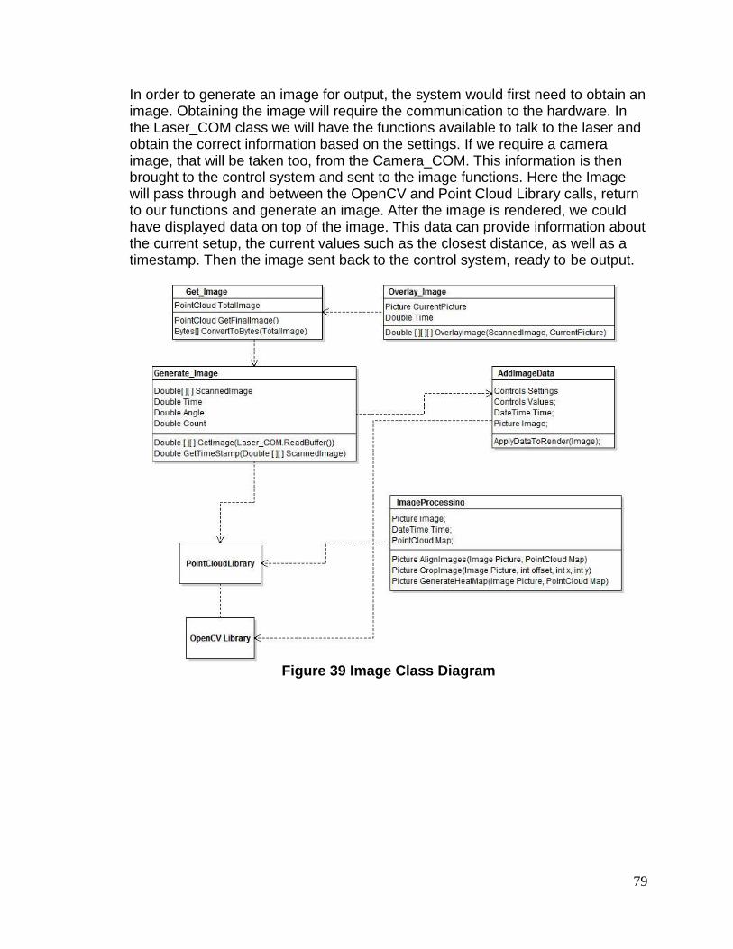
79

In order to generate an image for output, the system would first need to obtain an image. Obtaining the image will require the communication to the hardware. In the Laser_COM class we will have the functions available to talk to the laser and obtain the correct information based on the settings. If we require a camera image, that will be taken too, from the Camera_COM. This information is then brought to the control system and sent to the image functions. Here the Image will pass through and between the OpenCV and Point Cloud Library calls, return to our functions and generate an image. After the image is rendered, we could have displayed data on top of the image. This data can provide information about the current setup, the current values such as the closest distance, as well as a timestamp. Then the image sent back to the control system, ready to be output.

Figure 39 Image Class Diagram

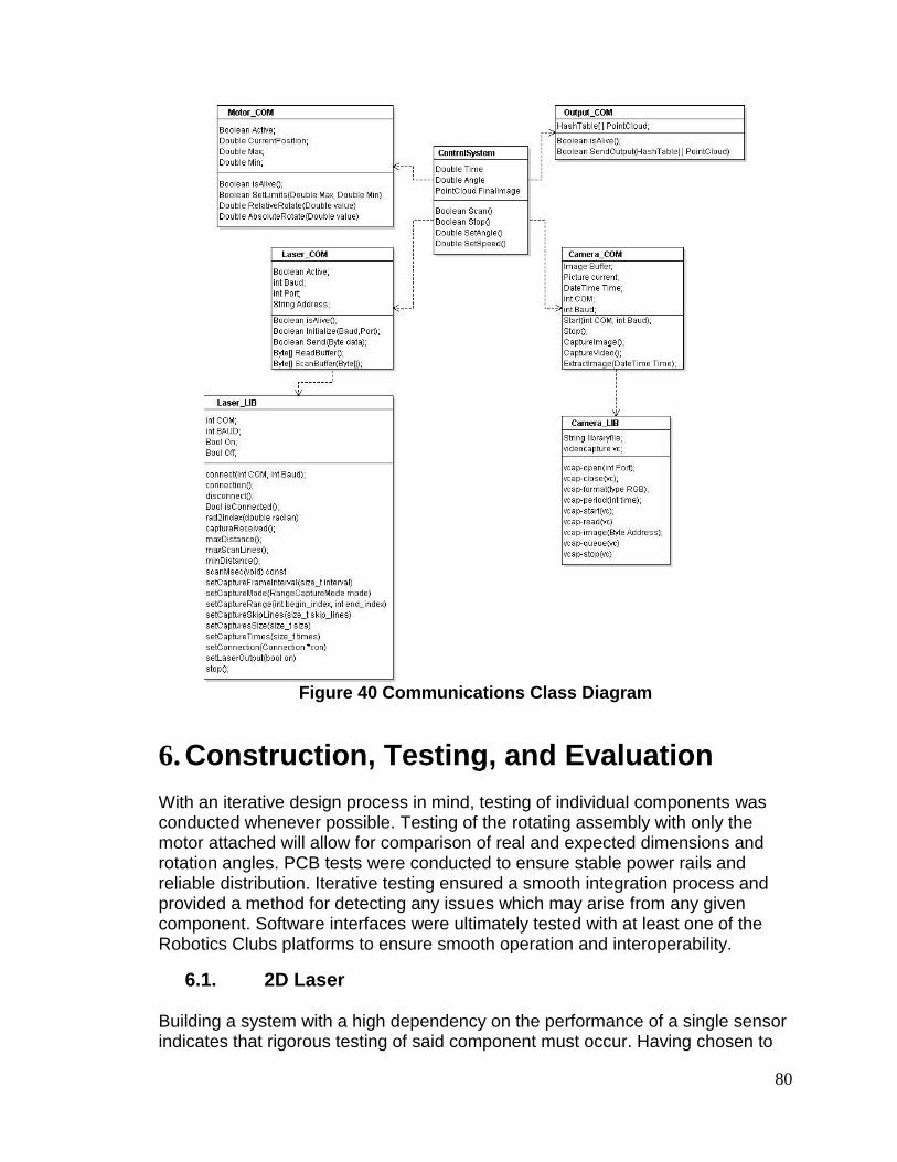
80

Figure 40 Communications Class Diagram

6. Construction, Testing, and Evaluation With an iterative design process in mind, testing of individual components was conducted whenever possible. Testing of the rotating assembly with only the motor attached will allow for comparison of real and expected dimensions and rotation angles. PCB tests were conducted to ensure stable power rails and reliable distribution. Iterative testing ensured a smooth integration process and provided a method for detecting any issues which may arise from any given component. Software interfaces were ultimately tested with at least one of the Robotics Clubs platforms to ensure smooth operation and interoperability.

6.1. 2D Laser Building a system with a high dependency on the performance of a single sensor indicates that rigorous testing of said component must occur. Having chosen to

81

use the Hokuyo UTM-30LX sensor due to its capability of outdoor (direct sunlight) operation the 2D performance characteristics of the sensor must be measured experimentally both inside and outside. Given the expected performance outlined by Hokuyo analysis of the actual performance of our exact sensor must take place. Performance metrics generated by experiment will greatly enhance overall 3D reconstruction accuracy and is a priority for evaluation. Testing was performed in both outdoor and indoor environments with a number of tests for determining distance accuracies in the full 270 degree field of view of the sensor. To reliably test measurement accuracy the testing surface and reflectivity (emissivity) must remain consistent across all tests. While it is impossible to have a true black body for a completely consistent testing platform any surface with a darkly colored matte surface proved reliable enough for testing in both indoor and outdoor environments. The test was to take measurements from a known location and then compare them with the laser data output. We found that the laser output data was accurate within fractions of centimeters.

Aside from measurement accuracies of the laser validation of other hardware features will be needed to validate complete operation. The hardware synchronization signal of the system gives the project the capability of faster processing of laser data. Given the event driven nature of the project the sync signal accuracy must be measured against expected update rates of the sensor. We validated the pulse times and duration within a specified window will allow for measurement of this signal to verify the projected update rate of 40 hertz.

6.2. Motor Upon receipt of the motor various aspects must be evaluated for verification of those advertised. Testing of the speed, torque, and encoder accuracies will be most vital. Testing of the motor was done in line with testing of motor communication from our microcontroller. This allowed for seamless transitioning during project construction and is the earliest time at which we can test the system. Using various load weights and protractors, load analysis and encoder accuracy were measured. With no viable method to evaluate max motor speeds, software measurements were used instead. This makes the accuracy of the encoder much more important than any other specification of the motor. Other physical facets such as weight and dimensions were examined to ensure proper weight distribution. Load testing was conducted in order to monitor actual power consumption on average and the effects on theoretical max speeds. Max power consumption was also tested as the batteries driving the system have maximum burst discharge rates which must be adhered to. We found that the motor was not actually going as fast as it reported. So in our code we have compensated for that speed adjustment and calculated actual speed based on real time timing data. The power tests proved to work within operating range and met all of our expectations as we never broke 2 amps even when holding a motor stall.

82

6.3. Microcontroller To ascertain that the microcontroller we have is operating properly all theoretical input and output functionality needed were examined. While typically certified before delivery as a consumer grade product it is was necessary to test base level operations before systems integration can occur. The RaspberryPi functioned properly based on the datasheets provided.

6.3.1. Power and Regulation Verifying proper power supply voltages and short circuit identification are the most basic forms of testing evaluation necessary for proper microcontroller operation. Using a digital voltmeter resistance we measured across all power rails to every ground pin to ensure that the value read is much greater than 0Ω. Upon successful completion of this testing, further visual inspection of the board for possible causes of shorts or broken traces was conducted. Assuming that all solder joints are full and complete further checks for possible manufacturer defects were needed. These checks verified that all soldered components including capacitors and resistors match those to the expected and designed values for the board. The regulators chosen for the PCB designed were chosen to be small, and many of them are surface mount based solutions. With our finished PCB, we soldered and tested each component as it went on the board. We tested for bridges, proper operating values, and other connectivity problems. Once we had the complete PCB soldered we tested and found that our voltage was a little low. So we adjusted our resistance value going into our regulator and brought our voltage up to our optimal voltage. Below is a list of all equipment required to carry out all of the hardware testing for the PCB and microcontroller.

Multi-meter

Oscilloscope

DC current meter

Logic analyzer

Microscope

6.3.2. Input and Output Microcontrollers provide many different forms of signal processing through on board circuits and hardware. Some signals may be converted between digital and analog via ADCs or DACS and others may be passed directly through from the MCUs themselves. Proper verification of these widely varying inputs and

83

outputs will provide the group with a uniform testing platform which can perform in the variety of environments expected of this system. Testing of the inputs and outputs of the MCU tested the following functionality at minimum: 1. Digital Input and Output 2. Analog Input and Output 3. PWM Signal Generation 4. TTL and Serial Connections 5. I2C and DACs Most output signals from the microcontroller were evaluated using the simplest of equipment, namely a multi meter and oscilloscope. Serial based communications involved more hardware as connections to physical devices need to be made in order to appraise two way communications. More expensive supplemental testing hardware such as signal generators and logic analyzers would enable the group to test in a more controlled fashion. The robotics club facilities provided the group with all necessary testing equipment for all signals into and out of the microcontroller.

6.4. Software Unit Testing Upon completion of the basic system capabilities including point cloud formation, 3D depth imaging, dynamic system configuration, and networking communication heavy software testing must incur to test all race conditions in the system. Reliability is the key of software unit testing and is a key component in any good development life-cycle. Below is a list of unit tests which were performed for the system to stress and verify all possible configurations work and do not throw unexpected errors or crash the laser’s operation. This testing also ensured full functionality of every component as the system is formulated. 1. Verify that the commands being set the PC side of the network are getting

changed on the 3D laser side.

2. Verify that setting changes do cause real-time closed loop control change of the continuous sweeping of the laser to accomplish the desired resolutions.

3. Test that a hard reboot of the system will not cause a total system failure

requiring a manual login to restart software applications. 4. Tests of multiple users on the same local network subscribing to the lasers

data does not interfere with operation or the receipt of other users of the data. 5. Verify that the microcontroller is capable of having the laser on a different

USB port without having to manually enumerate it.

84

6. Test that the output timing of the data adjusts to the resolution and the rotating range assigned to the laser.

7. Test each application in tandem to ensure proper permissions over the network as well as resource limitation.

8. Verify proper coordinate system transformation over the entire scanning range of the laser.

9. Test actual versus theoretical timing of the Hokuyo’s synchronization signal to test response time of interrupt driven application.

10. Tests setting motor shaft positioning with entire assembly mounted to ensure accurate control within tolerance of motor.

11. Testing of proper decay of point clouds over time as new scans are received.

12. Tests of 2D laser parameters and effects on 3D and other output data must be verified for consistency.

We were able to successfully perform all of the above tests at the completion of the project. We had to adjust the methods of communication in order to maintain he real-time ability. We also had to speed up laser and motor communication rates to allow for the most stable performance due to concurrency.

6.5. System Performance In order to create the best system, we analyzed the system under different conditions. Testing under the different conditions will allowed us to choose constraints for sensors, ideal readings for sensors, and other observable data that can be used in setting the default settings. In order to create code that can handle an issue, we must first have knowledge of the issue. This information can potentially have a dramatic effect on the method of operation in the software. The hardware may not need nearly as much alteration due to the fact that we are setting our constraints based on hardware and the environment.

6.5.1. Regular Environment Our 3D laser range finder can be used in a plethora of situations. Using the scanner in inside conditions will prepare the scanner for use in enclosed areas. “Inside” areas may include a large or small area. The differences between large and small areas can change the readings dramatically. If the sensor is in a room that is 10 meters x 10 meters x 10 meters, then it may be able to see the walls. If we are in a giant warehouse and the room is 100 meters x 100 meters x 100 meters, then the system may not be able to see the walls and we will need to know what that looks like.

85

The testing scenarios that will be utilized when testing under a regular environment are detailed in the following list:

1. A small room that is clear of any obstacles: This room will provide us with the ability to see how the system reacts to just seeing the walls of a room without any interference. During this test we collected the data and the feedback from this allowed us to alter the interpolation of points in a different manner. Once we tested again, we found our lines to be straight and have a perfect rendering of the environment. This acted as our baseline scan.

Figure 41 Camera Image of Clear Hallway

86

Figure 42 Point Cloud of Clear Hallway

2. A large room that is clear of any obstacles: Utilizing this type of scenario may allow us to see how the system reacts to an area that may not provide any feedback through our sensor. This could be considered null data and we would have to handle how this scenario plays out. We found that areas that reach beyond our 30 meter limit were unable to be seen and that our system would not return the points.

3. A small room that has a few small objects: Having just a few obstacles will allow us to test identifying objects. This could provide us information on how the system will identify and align imagery. This test showed us that we can successfully view objects in small room, however it shows that items that are closer cause further items to be unseen has it creates a larger shadow.

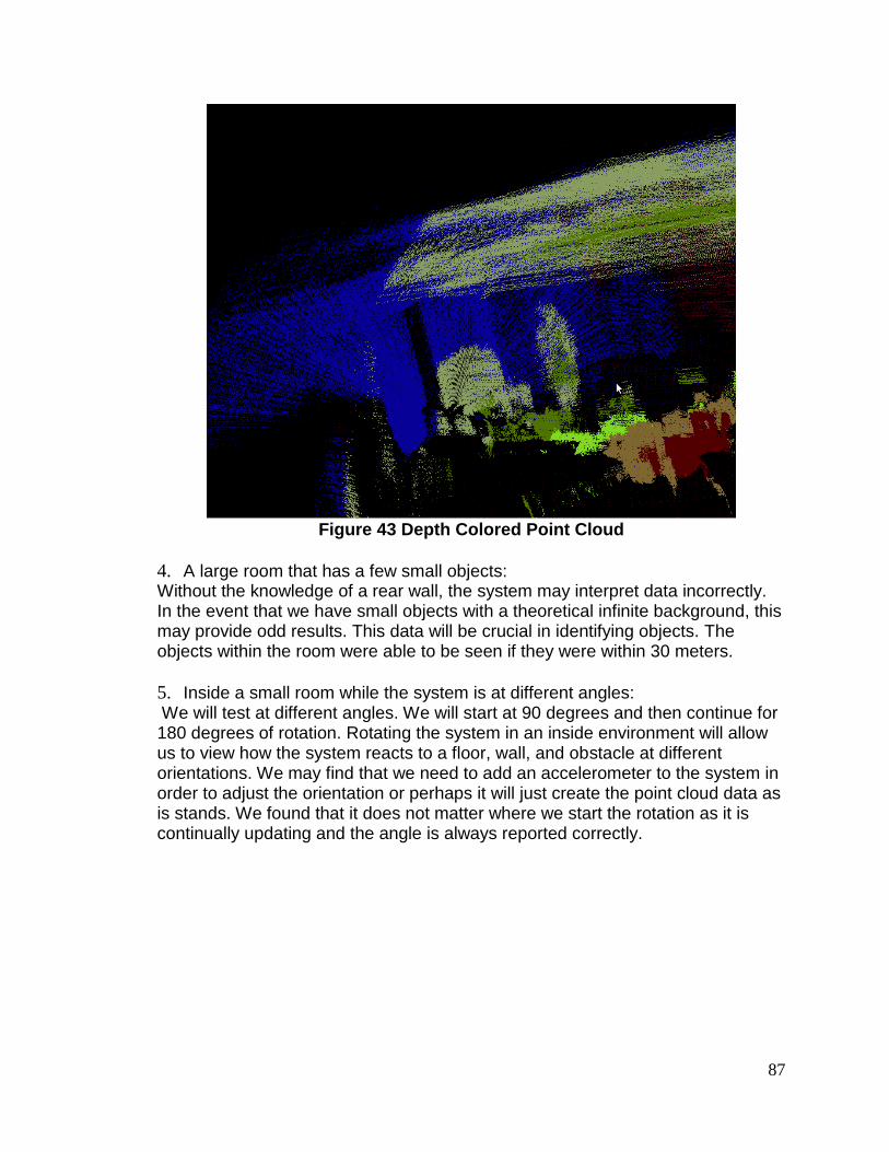
87

Figure 43 Depth Colored Point Cloud

4. A large room that has a few small objects: Without the knowledge of a rear wall, the system may interpret data incorrectly. In the event that we have small objects with a theoretical infinite background, this may provide odd results. This data will be crucial in identifying objects. The objects within the room were able to be seen if they were within 30 meters.

5. Inside a small room while the system is at different angles: We will test at different angles. We will start at 90 degrees and then continue for 180 degrees of rotation. Rotating the system in an inside environment will allow us to view how the system reacts to a floor, wall, and obstacle at different orientations. We may find that we need to add an accelerometer to the system in order to adjust the orientation or perhaps it will just create the point cloud data as is stands. We found that it does not matter where we start the rotation as it is continually updating and the angle is always reported correctly.

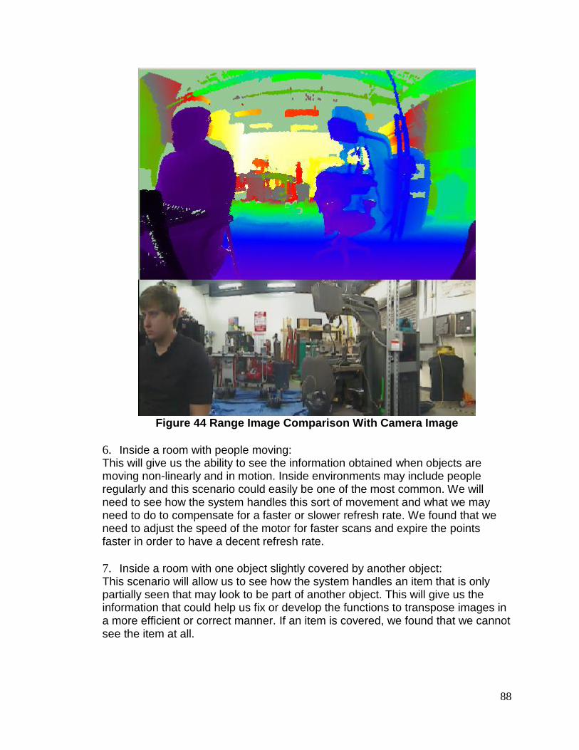
88

Figure 44 Range Image Comparison With Camera Image

6. Inside a room with people moving: This will give us the ability to see the information obtained when objects are moving non-linearly and in motion. Inside environments may include people regularly and this scenario could easily be one of the most common. We will need to see how the system handles this sort of movement and what we may need to do to compensate for a faster or slower refresh rate. We found that we need to adjust the speed of the motor for faster scans and expire the points faster in order to have a decent refresh rate.

7. Inside a room with one object slightly covered by another object: This scenario will allow us to see how the system handles an item that is only partially seen that may look to be part of another object. This will give us the information that could help us fix or develop the functions to transpose images in a more efficient or correct manner. If an item is covered, we found that we cannot see the item at all.

89

8. An object that moves progressively closer to the sensor: If an object is moving towards the scanner or the scanner is moving toward the object, then the size and depth of that object will change. We will need to document, test, and understand how this motion will read on our point cloud data. This system may create something that is skewed instead of normalized. Given a decent refresh rate on the client. It does not matter if an object moves closer as the point cloud only shows the latest possible data.

6.5.2. Outside Environment

The outside environment may cause another group of issues with our system. An outside environment is susceptible to additional conditions such as humidity, fog, lighting, rain, wind, and other weather conditions. Additionally there will be less uniformity in an environment when using the sensor outside versus an inside room. The following list is a few of the testing scenario for outside use.

1. Regular weather, normal sun: This test will give us a baseline for the remainder of our tests. The lighting alone could cause issues with our system and we may need to adjust our code if it realizes that the unit is being used outside. We found that the point cloud renders the same as indoors except there are far less points due to the sky being invisible.

Figure 45 Nighttime Scan Outside

90

2. Cloudy weather: We will run the system under different circumstances while the weather is cloudy. This will allow us to see if the laser sensor can take readings when the lighting is low. Same as regular weather testing, the clouds made no difference for our scans.

3. Rainy conditions: Rain is a tangible object and may be picked up on our laser sensor. Using our system in raining conditions may prove that a valid image may not be able to be created, or perhaps there is a way to counter this with an algorithm to remove the raindrops. Rain made some of the points disappear as well as some of the objects incomplete. The rain changes the reflectivity of an object and objects that are too reflective are not seen correctly.

4. Motion on uneven surfaces: We will move the sensor across an uneven area using a vehicular robot. This test will provide us the information when the scanner does not have a uniform ground level and may give invalid readings. We will need to know how this information looks so we can invalidate data or at least flag it as uneven. Motion on our client creates an odd image. It places objects in a position of existing objects until the full scan is updated. The client will need to utilize some type of motion sensor to make adjustments.

5. Many people moving: It is not uncommon for large groups of people to be moving around at a single location. This could be a walkway on the UCF campus. This test will demonstrate how the scanner can pick up moving objects of different speeds and we can see how it comes together. This may help us decide in default scanning values. This tested led us to have some “ghosting” as the images refreshed. However, it was able to see everyone in the image as long as they were visible.

6.5.3. Project Summary

Our 3D laser range finder will provide the ability to view an environment in 3D. This application can be used on many external systems as it will provide the eyes to any machine that decides to use it. Our system is robust, scalable, and successfully delivers the item requested by the Robotics Club at UCF.

91

7. Bibliography

[1] Lidar Output Protocol (http://asprs.org/a/society/committees/standards/asprs_las_format_v10.pdf)

[2] SM-42BYG011-25 Stepper Motor ( https://www.sparkfun.com/products/9238)

[3] 42BYGHM809 Stepper Motor ( https://www.sparkfun.com/products/10846 )

[4] A3967 Microstepping Driver ( https://www.sparkfun.com/products/10267 )

[5] STMicro's L6470 Stepper Motor Driver ( https://www.sparkfun.com/products/11611 )

[6] Hitec HS-805BB Servo Motor ( https://www.sparkfun.com/products/11881 )

[7] Dynamixel RX-24F Robot Actuator (http://www.trossenrobotics.com/dynamixel-rx-24F-robot-actuator.aspx )

[8] KM-12FN20-100-06120 DC Motor ( https://www.sparkfun.com/products/8910 )

[9] GB37Y3530-12V-83R DC Motor (http://www.robotmesh.com/12v-dc-motor-83rpm-w-encoder)

[10] E6A2-CS3E Rotary Encoder (https://www.sparkfun.com/products/10790)

[11] A6B2-CWZ3E-1024 Rotary Encoder (https://www.sparkfun.com/products/11102)

[12] PCL http://www.pointclouds.org

[13] SimpleCV (http://www.simplecv.org)

[14] PDAL (http://www.pointcloud.org/index.html)

[15] Communication (http://urgnetwork.sourceforge.net/html/index.html )

http://asprs.org/a/society/committees/standards/asprs_las_format_v10.pdf







http://www.trossenrobotics.com/dynamixel-rx-24F-robot-actuator.aspx


http://www.robotmesh.com/12v-dc-motor-83rpm-w-encoder

http://www.robotmesh.com/12v-dc-motor-83rpm-w-encoder



http://www.pointclouds.org/

http://www.simplecv.org/

http://www.pointcloud.org/index.html

http://urgnetwork.sourceforge.net/html/index.html

92

[16] UrgCtrl Laser Scanner Accessible Methods (http://www.hokuyo-aut.jp/02sensor/07scanner/download/urg_programs_en/classqrk_1_1UrgCtrl-members.html )

[17] Dynamixel RX-24F Robot Actuator Servo (http://www.trossenrobotics.com/dynamixel-rx-24F-robot-actuator.aspx)

[18] Camera (http://www.raspberrypi.org/phpBB3/viewtopic.php?f=43&t=50639)

[19] ASPRS (http://asprs.org/a/society/committees/standards/asprs_las_format_v10.pdf).

[20] OpenCV

(http://docs.opencv.org/modules/refman.html)

[21] RPi Hardware Access (http://elinux.org/Rpi_Low-level_peripherals)

[22] RX-24F http://support.robotis.com/en/techsupport_eng.htm#product/dynamixel/rx_series/rx-24f.htm

[23] TI LMZ14203 http://www.ti.com/product/lmz14203

[24] TI LM7805CV https://www.sparkfun.com/datasheets/Components/LM7805.pdf

[25] CUIINC V78-2000 http://www.cui.com/product/resource/v78xx-2000.pdf

[26] Hokuyo PBS http://www.hokuyo-aut.jp/02sensor/07scanner/pbs.html

[27] URG-04LX-UG01 http://www.hokuyo-aut.jp/02sensor/07scanner/urg_04lx_ug01.html

[28] URG-04LX

(http://www.hokuyo-aut.jp/02sensor/07scanner/urg_04lx.html)

[29] Hokuyo UTM-30LX (http://www.hokuyo-aut.jp/02sensor/07scanner/utm_30lx.html)

[30] Sparkfun Images http://creativecommons.org/licenses/by-nc-sa/3.0/

http://www.hokuyo-aut.jp/02sensor/07scanner/download/urg_programs_en/classqrk_1_1UrgCtrl-members.html



http://www.trossenrobotics.com/dynamixel-rx-24F-robot-actuator.aspx

http://www.raspberrypi.org/phpBB3/viewtopic.php?f=43&t=50639



http://docs.opencv.org/modules/refman.html

http://elinux.org/Rpi_Low-level_peripherals

http://elinux.org/Rpi_Low-level_peripherals

http://support.robotis.com/en/techsupport_eng.htm#product/dynamixel/rx_series/rx-24f.htm

http://support.robotis.com/en/techsupport_eng.htm#product/dynamixel/rx_series/rx-24f.htm

http://www.ti.com/product/lmz14203

https://www.sparkfun.com/datasheets/Components/LM7805.pdf

http://www.cui.com/product/resource/v78xx-2000.pdf

http://www.hokuyo-aut.jp/02sensor/07scanner/pbs.html

http://www.hokuyo-aut.jp/02sensor/07scanner/pbs.html

http://www.hokuyo-aut.jp/02sensor/07scanner/urg_04lx_ug01.html

http://www.hokuyo-aut.jp/02sensor/07scanner/urg_04lx.html

http://www.hokuyo-aut.jp/02sensor/07scanner/utm_30lx.html

http://creativecommons.org/licenses/by-nc-sa/3.0/

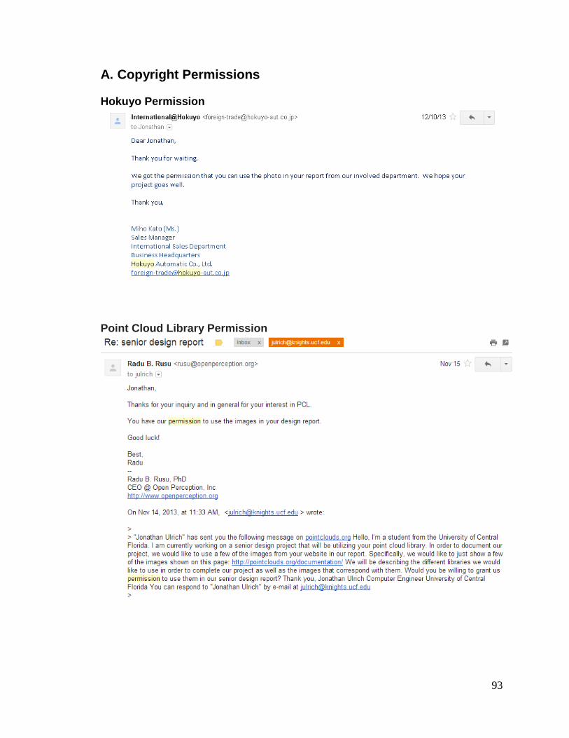
93

A. Copyright Permissions Hokuyo Permission

Point Cloud Library Permission

94

Sparkfun Usage License


TI Permission

Fair Use Policy http://www.youtube.com/yt/copyright/fair-use.html


http://www.youtube.com/yt/copyright/fair-use.html

Documents

Pidar: 3D Laser Range Finder