Embed Size (px)
Citation preview
IZA DP No. 1593
Piecework versus Timework inBritish Wartime Engineering
Robert A. Hart
DI
SC
US
SI
ON
P
AP
ER
S
ER
IE
S
Forschungsinstitut
zur Zukunft der Arbeit
Institute for the Study
of Labor
May 2005
Piecework versus Timework in
British Wartime Engineering
Robert A. Hart University of Stirling
and IZA Bonn
Discussion Paper No. 1593 May 2005
IZA
P.O. Box 7240 53072 Bonn
Germany
Phone: +49-228-3894-0 Fax: +49-228-3894-180
Email: [email protected]
Any opinions expressed here are those of the author(s) and not those of the institute. Research disseminated by IZA may include views on policy, but the institute itself takes no institutional policy positions. The Institute for the Study of Labor (IZA) in Bonn is a local and virtual international research center and a place of communication between science, politics and business. IZA is an independent nonprofit company supported by Deutsche Post World Net. The center is associated with the University of Bonn and offers a stimulating research environment through its research networks, research support, and visitors and doctoral programs. IZA engages in (i) original and internationally competitive research in all fields of labor economics, (ii) development of policy concepts, and (iii) dissemination of research results and concepts to the interested public. IZA Discussion Papers often represent preliminary work and are circulated to encourage discussion. Citation of such a paper should account for its provisional character. A revised version may be available directly from the author.

IZA Discussion Paper No. 1593 May 2005
ABSTRACT
Piecework versus Timework in British Wartime Engineering∗
The British engineering industry experienced extreme production and employment pressures during the rearmament period that preceded the Second World War and in the early war years. Did it react by placing a greater emphasis on incentive-compatible payment methods? This paper examines the relative employment and wage effects on pieceworkers and timeworkers. Empirical work is based on detailed firm-level payroll data produced by the Engineering Employers Federation covering the period 1935 to 1942. The paper investigates the effects of war on piecework and timework in relation to (a) labour market arguments concerning substitution between payment methods, (b) piece rate/time rate adjustments to changes in product demand, (c) relative changes in employment and hours, and (d) relative changes in hourly and weekly pay. JEL Classification: J31, J33, N34, N44 Keywords: piecework, timework, British engineering, World War II Corresponding author: Robert A Hart Department of Economics University of Stirling Stirling FK9 4LA Scotland UK Email: [email protected]
∗ Data collection and empirical work was funded by ESRC Grant RES-000-22-0491. I am grateful to the Engineering Employers Federation for allowing access to their payroll statistics and to Warwick University Modern Record Centre and Glasgow University Archive Services for their help in assembling the material. Adele Redhead was especially helpful at Glasgow. Thanks also to Andrew Currall, Lucy Burrows and Elva McLean for work on transcribing data from EEF archives to computer spreadsheets. Elizabeth Roberts provided excellent research assistance.
1 Introduction Empirical work based on specific case studies has found quite sizeable productivity gains
when comparable workers operate under a piece rate rather than a time rate pay system
(Lazear, 2000; Paarsch and Shearer, 2000). It is also well established that pieceworkers
enjoy higher earnings relative to timeworkers (see also Pencavel, 1977 and Seiler, 1984).
Yet piecework is by no means the dominant payments system in national labour markets.
Piecework tends to have a comparative advantage where it is relatively inexpensive to
measure and monitor individual contributions to output and to operate quality control
systems. Unsurprisingly, therefore, there is a relatively high incidence among manual
workers. Pencavel (1977) shows that between 1947 and 1961 at least 40 percent of
British male manual workers in metal manufacture, shipbuilding and marine engineering,
vehicles, and other metals and engineering worked on a payments-by-results basis.
Concentrating on manual workers in British engineering, this paper examines the impact
of the Second World War on the relative incidence, hours of work and pay of
pieceworkers and timeworkers. This is an especially interesting period because it
produced acute pressures on the industry to switch towards incentive-based payments
systems.
Given relatively stable macroeconomic growth over a prolonged period, we might
expect that the incidences of piecework and timework would not vary greatly. Product
type, production methodology, labour quality and work organisation may combine to
make piecework the more cost effective remuneration system. Other combinations may
favour timework. Trend changes towards one system or the other would be expected to
follow major, relatively long-term, innovations in product development, technological
1
know-how, employee training, and organisational structure. 1 A comparative advantage
to studying wage systems in war-affected years is that major changes took place over a
short period of time. Extreme demand for war-related engineering products, exacerbated
by acute skill shortages, gave rise to a set of economic circumstances that forced many
engineering companies to change radically their worker skill inputs and methods of
production. The issue of piecework versus timework featured prominently within this
reorganisation.
Section 2 outlines briefly the growth of the engineering industry in the run-up to
war and during the war years. Labour market arguments concerning the relative
employment and pay of pieceworkers and timeworkers during this important episode of
economic history are presented in Section 3. Sections 4 to 7 report related empirical
findings based on a unique data set produced by the Engineering Employers Federation
(EEF). Wages and hours statistics were compiled from the payroll records of affiliated
member firms. The Federation’s membership was highly representative of the industry as
a whole. In 1940, there were over 2000 engineering firms in the EEF, employing about 1
million workers and covering all sections of the industry (see Marsh, 1965, p.48). Payroll
statistics of member firms were systematically collated largely for the purposes of
providing employers with critical information during national level bargaining with
1 If we take the period from the end of the Second World War to the late 1950s/early 1960s as a relatively stable period, Pencavel (1977) shows modest changes in the incidence of payments-by-results among U.S. production workers and among British female manual workers. By contrast, there was significant growth in the incidence of payments-by-results among British male manual workers; for example, the percentage of manual workers in metal manufacture grew from 50 percent to 62 percent between 1947 and 1961. However, in ‘other metals and engineering’ the classification nearest to the data studied here, the percentage rose very slightly from 44 to 45 percent. Pencavel also reports evidence that no discernible new British patterns of piecework incidence arose between 1961 and 1967.
2
engineering unions. Data cover engineering occupations, engineering sections and
geographical EEF districts between 1935 and 1942. All data are provided separately for
pieceworkers and timeworkers. I concentrate on male workers. Section 4 examines the
relative sensitivity of piece rates and time rates to demand changes during the run-up to
war. Section 5 reports on changes in the incidence of pieceworking over the period and
on the weekly hours of workers under the two payments regimes. Section 6 analyses
piecework/ timework earnings differentials, embracing both wage rates and hours.
Section 7 highlights the effects of the exceptional labour market pressures on piece rates
in Coventry relative to other engineering districts. Main findings are summarised in
Section 8.
2. Engineering growth between 1935 and 1942
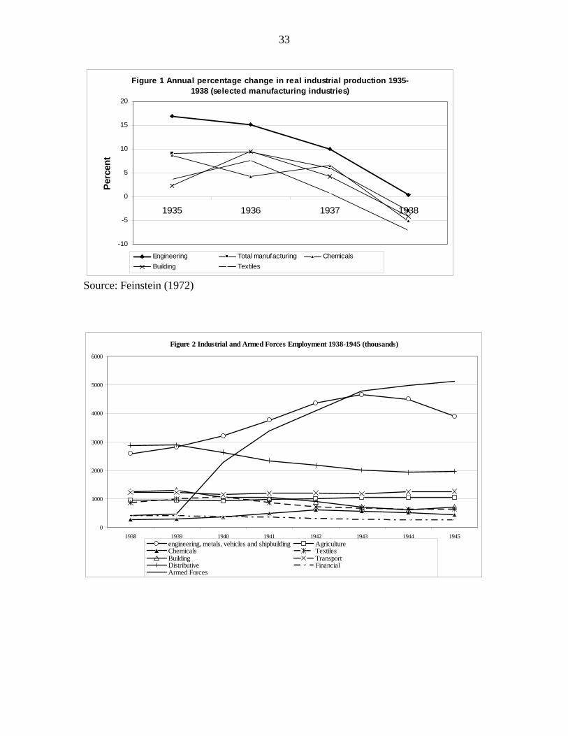
Starting in 1935, a series of rearmament programmes acted as catalysts for major
expansions of Britain’s engineering sector (Inman, 1957, Chapter 2). Annual percentage
increases in real production of 17, 15 and 10 percent occurred in 1935, 1936, and 1937,
respectively. Figure 1 shows production expansion in the run-up to war was significantly
higher in engineering than either in manufacturing as a whole or in other major one-digit
industries. During the war years there was a considerable growth of employment in
engineering and closely related industries. Between 1938 and its peak in 1943,
employment in engineering and allied industries (metals, vehicles and shipbuilding) grew
by 80 percent (from 2590 thousand to 4659 thousand employees). Figure 2 shows that
steep employment increases in this group of industries together with the armed forces
contrasted markedly with flat or declining employment elsewhere. Growth in product
demand and employment was by no means evenly spread across engineering sections and
3
geographical engineering districts, however. For example, pressure was especially
intense in aircraft manufacture and in associated local labour markets such is the
Coventry area.
e
Several well know
Ministry of Labour and N
derived from engineering
Depression as well as from
relatively high wages. As
materials and managemen
from outside firms throug
aircraft manufacture (Inm
weekly hours per worker
As the pressures o
were radically revised. Br
broken down into compon
relatively short training pe
identified as suitable for s
automatic and semi-autom
re-classification was univ
2 Dilution is not especially a wdefined under broadly-based skInstead, they were broken dowskilled workers and semi-skille
Figures 1 and 2 her
n sources of increased labour input are documented in the
ational Service (1947) and Inman (1957). Employment growth
workers returning to the industry following the Great
workers who were attracted from other industries by
engineering firms in key locations faced plant, capacity,
t constraints, there was an increased tendency to employ labour
h sub-contracting. The latter was especially important in
an, 1957, pp.24/5). On firms’ intensive margins, average
grew dramatically during war-affected years (see Section 5).
f war preparation and execution intensified, production methods
oad work areas traditionally covered by skilled workers were
ent job tasks. Semi-skilled workers were trained over
riods in order to perform some of these tasks. Other tasks were
emi-skilled work per se. The development and application of
atic machines helped greatly in this latter respect. This work
ersally referred to as labour dilution (see Parker, 1981).2 In the
ell-chosen term. It is meant to convey the fact that a coherent set of job tasks illed trades increasingly ceased to be performed by single individuals.
n (or diluted) into sub-sets of tasks and shared among more narrowly trained d workers. But in important respects this process provided for better
4
early war years dilution involved a significant expansion of female jobs: females
accounted for 10 percent of total engineering employment in 1939, a figure that rose to
35 percent by 1943. From 1940, female engineering workers were classified into two
groups: ‘women doing men’s work’ and ‘women doing women and boys work’. The
former group undertook a 32 week training period that allowed them to undertake skilled
and semi-skilled job tasks in vital wartime sectors such as aircraft manufacture and heavy
general engineering (Hart, 2004).
Apart from increasing the stock and utilisation of labour input, there was another
potentially important method of meeting output requirements. This was to induce greater
productive effort by substituting towards incentive-based pay. This is the focus of
attention here. Throughout the 1920s and 1930s, both piecework and timework comprised
important components of work activity throughout most sections of the engineering
industry (Knowles and Hill, 1954). Piecework represented a high proportion of total
labour input in sections like aircraft manufacture, electrical engineering and heavy
general engineering. Timework was relatively more prevalent in marine engineering,
sheet metal working and light general engineering. The critical questions in this paper
concern the marginal effects of war on the relative workforce sizes, working time and pay
of the two groups.
3 Piecework versus timework under the pressure of war demand
This section discusses a number of war-related issues that would be expected to
influence the relative incidence and remuneration of piecework and timework. At the end
matches between skill and work requirements. For example, increasingly scarce highly skilled workers could now concentrate their work effort purely on tasks that demanded the most experience and know-how.
5
of the section, the key points are summarised and form the basis of the subsequent
empirical investigation.
At the outset, it is useful to distinguish between the weekly wage earnings of
timeworkers and pieceworkers. To simplify, overtime premium payments are ignored.
Wage earnings of a timeworker, yT, simply consists of an hourly wage rate, wT, multiplied
by the length of weekly hours, hT: that is
(1) yT = wThT.
By contrast, weekly earnings of a pieceworker are dependent on weekly output. In
principle, a piece rate represents payment for the time taken by a ‘typical’ worker to
complete a specified job task by applying ‘normal’ hourly effort. Piece rates could be set
independently by ‘time and motion’ engineering experts although, as we will see, this
was not the only infuence on rates setting. Following Pencavel (1977), the weekly
earnings of a piecworker, yP, is represented by applying an index, dependent on hours and
effort, to the piece rate. This is expressed
(2) yP
= pΦ[hP, e]
where p is the piece rate, Φ is an incentive payments index predicated on a pieceworker’s
weekly hours, hP, and hourly effort, e.
(a) Pay responsiveness to market conditions
Piecework offered British engineering employers the potential to achieve
relatively high wage flexibly in the face of exceptional wartime demand and supply
dynamics. This was especially attractive at a time of extreme labour scarcity in core
6
engineering districts and sections where it became imperative both to prevent quits
among the existing workforce and to attract new recruits from elsewhere. While there
was scope for firm-level time rate adjustments, the levels and occupational distributions
of time rates (i.e. wT in (1)) were subject to considerable national-level influence.
Essentially, all EEF annual time rates were based on national bargains struck with respect
to just two occupations.3 Pieceworkers’ earnings were settled primarily by company-
level bargaining (Knowles and Hill, 1954). There was some attempt at Federation-level
to established a percentage relationship between the basic time rate and the least that a
pieceworker of average ability could expect to earn.4 Predominantly, however,
piecework remuneration were settled at local level, with a great complexity of payments
within and between engineering sections due to (i) the need to set a vast number of
piecework prices and related job task execution times, (ii) wide variations in the methods
of arriving at agreed piece rates and (iii) a lack of experience of how to set piece rates in
wartime product demand conditions
Why would we expect more flexible market responses among pieceworkers
earnings? First, it was much harder to control and monitor piece rates than time rates.
“Owing to the immense number of different processes and operations in so heterogeneous
an industry, as well as to the rapidity of technical developments, any general control over
piece-work earnings can be no more than minimal” (Knowles and Hill, 1954). Second,
3 National rates were negotiated in respect of fitters and labourers. From 1922, nationally agreed rates applied uniformally throughout the Federation in Britain. Rates for other occupations were then related to one or other of these two occupational groups, again involving large elements of national agreements. 4 This was set at 25 percent between June 1931 and March 1943 and 27.5 percent until November 1950. A further national level agreement involving both payment methods was that both timeworkers and pieceworkers received a so-called National Bonus throughout this period. Pieceworkers received a lower Bonus than timeworkers.
7
wartime deskilling was achieved by job task compartmentalisation and simplification.
This improved employers’ abilities to monitor work performance and allowed greater
control of effort levels to meet prevailing demand conditions. Through (2) this directly
impacted on pieceworkers’ earnings. Third, as argued by Knowles and Robertson (1951a)
unfamiliarity with the special demands of war supply prevented accurate piece rate
pricing. This offered considerable scope for gearing piece rates towards alleviating acute
labour market pressures – especially attracting and retaining scarce labour - rather than
reflecting systematic engineering-based ‘time and motion’ price setting.5
Pay flexibility outside of national agreements was also possible in relation to
timeworkers, especially in the form of special merit awards, bonuses and lieu rates.
(Overtime hours and bonuses applied to both pieceworkers and timeworkers.) But it
remains highly likely – and certainly worthy of empirical investigation – that piecework
offered the greater pay responsiveness to the pressures of wartime output demand
together with the associated shortages of skilled labour supply.
(b) Piecework and timework under tight labour market conditions
The engineering labour market was especially tight in the years marking the run-
up to and the early period of war. Two arguments in the existing literature support the
view that this market condition itself would give rise to a greater emphasis on piecework.
The first concerns the value of piecework in relation to the outside wage (Lazear,
1986). The better are the opportunities in outside employment, the greater are the losses
incurred by the firm in failing to sort and remunerate workers by value added. So the
5 A 1949 study into the problems of measuring and comparing productive performance across different engineering plants (Joint Committee of the Institute of Production Engineers and of the Institute of Cost and Works Accountants) highlighted the common practice of ‘padding’ engineers’ estimates of the speed and effort required to complete job tasks in order to make wage earnings more attractive.
8
value of piecework would rise relative to timework. Extreme labour shortages of skilled
labour in the late 1930s/early 1940s – especially in the British Midlands – produced
intense competition among engineering companies in respect of their demands for key
workers.
“In any district firms could attract labour from other factories by adjustments in piece rates, the offer of merit bonuses or of overtime. As skilled labour grew scarcer and the number of new factories increased, poaching became steadily worse…..Firms spent hundreds of pounds advertising for skilled workers while those already in their employment sometimes left as fast as new men were recruited. Labour costs increased out of all proportion to increases in output; indeed long hours, high labour turnover and high piece rates tended to bring individual output down” (Inman, 1957, p.26).
In other words, the value of the alternative wage grew relative to the value of output in
the current firm. Therefore, firms perceived the advantage of offsetting higher job quit
probabilities among their most productive workers by directly rewarding individual value
added.
The second argument is also related to outside opportunities, but this time in
relation to worker motivation and incentives. In the face of exceptional demand
pressures, the employer is especially keen to motivate the workforce to provide
commitment and effort on the job. But the effectiveness of the sanctions available in the
case of timeworkers is inversely related to the degree of labour market tightness. Threat
of dismissal in the event of shirking, for example, has potentially little impact if the
worker has many alternative job opportunities. Under these circumstances, Macleod and
9
Malcomson (1989) show that the employer will tend to switch to piecework contracts as a
means of worker motivation.6
(c) Ability, labour heterogeneity and pay differentials
Why in general is there a positive gap between the hourly pay of pieceworkers
and timeworkers, ceteris paribus? Why might the gap be expected to widen during the
war period?
One major reason for the wage gap is that time working firms employ workers of
lower average ability (Lazear, 1986; Brown, 1990). Suppose that there is a zero-profit
equilibrium and that information is asymmetric in that workers are better informed than
firms about their output potential.7 For wide enough disparities in ability and given
positive monitoring costs, it may be worthwhile economically for low ability workers to
match with firms that do not incur those costs. (The wage of a low ability pieceworker
would not only reflect productive performance but also the cost of monitoring that
performance.) Such firms pay time rates and these rates would reflect the propensity to
attract workers of relatively low ability.
Why might the gap be expected to widen as the war progressed? Following
Lazear (1986), suppose managers and workers have a symmetric lack of knowledge
6 Another situation in which a threat of dismissal would lose its potency is when a worker nears the age of retirement. Gibbons and Murphy (1992) use the argument to explain the growing importance of incentive contracts towards the end of the careers of chief executive officers. 7 The work of Lazear (1986) and Brown (1990) compare piece rates and salaries. The latter imply that per-period earnings are fixed. This is tantamount in the present context to assuming that time-rated engineers worked fixed length workdays or weeks. Since, as is shown below, weekly hours of engineering workers changed greatly over this period the results reported in this Section are strictly first-approximations to expected outcomes. The earlier work also distinguishes between variations in individual ablility for given effort and variations in effort for given ability. Theoretical outcomes are comparable in most cases. Fama (1991) presents an interesting discussion of the distinction between hourly wages (as experienced by time-rated manual engineers) and salaries. It is argued that time payoffs (e.g. hourly wages) require information about hourly effort and/or output while salary payoffs occur when there is a lack of knowledge of effort and output flows.
10
concerning individual ability. In the short run, time rates are independent of output.
Therefore, timeworkers incur no monitoring costs in contrast to pieceworkers.8 But,
unlike piecework, timework involves costs arising from a failure to sort workers by
individual value-added. If costs associated with labour heterogeneity rise relative to costs
of monitoring performance then the value of piecework relative to timework is enhanced.
As reported in Section 2, labour heterogeneity increased as a direct result of
deskilling in the industry. The identification of more narrowly defined sets of job tasks
allowed companies, after providing relatively short periods of training, to upgrade semi-
skilled workers to undertake previously defined skilled work. The substitution of male
by female workers was an important element of this latter process (Hart, 2004). The
general consequence was to introduce more heterogeneous ability levels in the
manufacture of specific engineering products. As a consequence, there would have been a
rise in the implicit costs of failing adequately to sort workers by their contribution to
output.9 In other words, the process of deskilling served to increase the relative returns to
operating piece-rated payments systems.
The U.S. empirical investigation of Brown (1990) supports this line of reasoning.
Based on the Industry Wage Survey of the Bureau of Labor Statistics, it is found (p.180S)
that “there is less use of incentive pay (and greater use of standard rates) in jobs with
8 There is an important distinction to be made here, however. A piece rate system necessitates the allocation of more resources geared to inspecting the quality of output. Time rated work, however, generally associates with high costs of supervision in order to minmise shirking (Pencavel, 1977). Monitoring costs in the main text refer to the first of these two costs. 9 The problem of widening employee ability was formally recognized in employer-union agreements in relation to wage differentials between males and substitute female ‘dilutees’ (Inman, 1957, pp. 57-60 ). After a period of training, equal pay for equal work was the underlying principle. In practice, agreements allowed male-female wage differentials to persist where it was deemed necessary to provide female workers with extra long-term assistance and supervision. It should be added that these latter conditions were difficult to interpret and proved to be quite contentious.
11
diverse duties than in jobs with unchanging duties repetitively performed”. The process
of deskilling – aided and abetted by an increased use of automated machines - tilted the
balance far more towards job tasks involving repetitive work activities.10
Not only did deskilling in the industry increase the worth of measuring and
rewarding individual outputs but it also served potentially to enhance the productivity of
pieceworkers since it enabled the firm to improve performance monitoring within the
simplified job tasks.11 To the extent that productivity effects were reflected in pay then
wage differentials of pieceworkers and timeworkers would be expected to be directly
linked to labour heterogeneity.
(d) Noisy output
Several of the foregoing arguments point firmly to an expected substitution of
piecework for timework during war activity. There is an offsetting argument, however.
As discussed by Pencavel (1977) and Lazear (1986), a piece rate system may be
disadvantaged if there is a constant need to undertake frequent revisions of piece rates
and job-execution times. As stated by Lazear (p.411): “Piece rates are less likely to be
chosen when the estimate of [output] is noisy”. Time rates avoid the costs of assessing
and undertaking relative rapid price changes across an individual’s range of job tasks.
Knowles and Robertson (1951b) use the term, ‘tight’ piece rates, to describe long periods
of product price stability in which ‘equilibrium’ piece rates can be determined and
administered. By contrast, these authors argue that ‘loose’ piece rates prevailed in
10 See Cowling (2001) for reported research into the positive associations between payments by results and repetitive jobs and negative associations between payments by results and jobs with a wide range of tasks. 11 For empirical evidence on a positive relationship between payments by results and labour productivity see Heywood, Siebert and Wei (1997).
12
wartime engineering because rapid price fluctuations brought about by war demand
pressures (see Figure 7 below) precluded full assessments of appropriate relative prices.
Summary
The above discussion leads to the following testable propositions.
(i) The facts that piece rates were harder to control than time rates, improved
monitoring due to deskilling enhanced employers’ abilities to influence
productive effort, and unfamiliarity with wartime demand allowed greater
freedom over piece rate setting lead to the expectation that earnings of
pieceworkers were more responsive to market conditions.
(ii) On the basis of three main arguments – concerning labour scarcity and
potential quit threats, incentive compatible pay in tight markets, and improved
monitoring due to deskilling - we would expect the proportion of
pieceworkers relative to total workers to increase during the war period.
However, a fourth argument linked to noisy output serves to offset this
tendency.
(iii) In line with most other studies, and not necessarily related to war activities per
se, we would expect a positve gap between the pay of pieceworkers and
timeworkers due to differential abilities.
(iv) To the extent that piece rate - time rate differentials reflect relative
productivity we would expect a wartime widening in the differentials linked to
greater labour heterogeneity.
These arguments omit one additional important variable that affected both
employment and pay – viz. average weekly hours of pieceworkers and timeworkers. For
13
example, would the expected relative growth of numbers of pieceworkers be
accompanied by a relative growth in pieceworkers’ relative weekly hours? How did
hours combine with wage rates and piece rates to influence earnings differentials? The
associated role of working time is also investigated in what follows.
4 Relative wage responsiveness to market conditions
As noted in Section 3(a), the adoption of piece rate systems may have been
attractive to employers if piecework earnings offered relatively greater pay flexibility.
Wage responsiveness in certain engineering sections and geographical districts was
especially important given that it was necessary to establish significant short term wage
differentials in order to allow companies to overcome exceptional labour shortages.
Some insights into the relative demand elasticities of piece rates and time rates
can be obtained from two sets of data. The first covers the re-armament years from 1935
to 1938 and is based on males in 15 engineering occupations12 and twenty geographical
districts.13 The second involves a single occupation group, skilled male fitters, and
covers the longer period, 1926 – 1938. For both data sets, the 1938 end-date is
conditioned by the availablity of district-level unemployment rates that match EEF
geographical districts (obtained from Hart and Mackay, 1975). Also, I concentrate on
real basic wage rates so as to avoid complications linked to differential overtime working.
I adopt the wage curve specification of Card (1995) and concentrate on
pieceworkers’ real standard hourly wage, wP, in respect of the first data set to illustrate 12 These are coppersmiths, fitters (other than skilled), fitters (skilled), toolroom fitters, labourers, machinemen (rates at or above fitter’s rate), machinemen (below fitter’s rate), machine moulders (at or above moulder’s rate), machine moulders (below moulder’s rate), moulding machine operators, moulders (loose pattern), patternmakers, platers/riveters/caulkers, sheet metal workers, and turners. 13 Aberdeen, Barrow, Bedfordshire, Birmingham, Bolton, Burnley, Coventry, Derby, Dundee, Halifax, Leicester, Lincoln, Liverpool, London, Manchester, North East Coast, Preston, Rochdale, Sheffield, Wigan.
14
the methodology.14 Averaging over all pieceworkers by occupation i in district r at year
t, the underlying wage specification is given by
(3) irttrrt
Pirt efdauw +++=log
where urt is the district unemployment rate, a is a constant and where dr and ft are district
and time intercepts. First differencing (3) removes district fixed effects, giving
(4) irttrtrt
Pirt eguauaw ∆+++=∆ −121log
where gt represents the reformulated time intercepts after differencing. If in (4) a1 is
found to be significantly negative and a2 insignificant then this provides empirical
support for the Phillips curve. Alternatively, if estimates of a1 and a2 display equal sized
parameters with opposite signs then a wage curve is accepted.
The district unemployment rate in (4) does not differentiate between occupation
groups. Within a given district different groups may share common components of
variance that are not captured by a single rate. This may serve to bias downwards the
estimated unemployment standard errors (Moulton, 1986). In order to tackle this
problem, I extend the two-step estimation approach of Solon et al. (1994) to include
cross-section unemployment variation. Step 1 consists of estimating the equation
(5) ∑∑= =
+=∆T
t
R
rirtrtrt
Pirt uDUMw
1 1log φ
14 EEF data allow us to obtain estimates of weekly pay in (2) based on a standard workweek (i.e. excluding overtime hours). Hourly standard pay, wP, is then obtained by dividing this weekly total by 47, the length of weekly standard hours that applied to all workers in the industry.
15
where, summing over all T time periods and R districts, DUMrt denotes a dummy variable
that takes the value of 1 for district r at year t. In step 2, estimates of φrt in (3) are
regressed on unemployment rates plus district and time intercepts, that is
(6) .ˆ
121 rttrrtrtrt vfdubub ++++= −φ
This two step estimation procedure is also carried out separately with respect to
timeworkers’ (log) real wages, log wT.
For the second data set, based on a single-occupation, only equation (4) is
estimated.
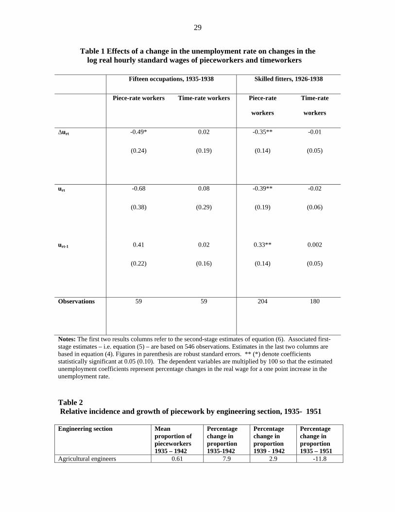
e
Ordinary Least Squares e
results, a significant coefficient o
pieceworkers’ equations. A one-
with a 0.49 percent increase in th
estimated over 15 occupations an
single occupation. Separating cu
wage curve specification in the la
the 5 percent level in the former.
modest, the contrast markedly wi
timeworkers do not support an as
and unemployment rates.
Table 1 her
stimates are reported in Table 1. For both sets of
n the change of unemployment is obtained only in the
point decrease in the rate of unemployment is associated
e real standard hourly wage in the 1935-38 time series
d a 0.35 percent increase in the 1926-38 series for a
rrent and lagged unemployment produces support for a
tter regression while the two rates are insignificant at
While the estimated piece rate elasticities are relatively
th the time rate equivalents. Both sets of results for
sociation between changes in real basic hourly wages
16
The comparative findings in Table 1 are in line with work on more recent U.S.
data by Devereux (2001). This emphasises the need to discriminate among types of
payment methods in the study of wage cyclicality. Compared to earlier micro longitudinal
studies, but ones that have not conducted wage disaggregation, Devereux finds relatively
weak cyclicality. A marked exception is the finding of strong wage procyclicality among
workers receiving incentive-based pay. The latter comprise a residual group in the Panel
Study of Income Dynamics, comprising individuals compensated by "piece rates,
commissions, tips, and in other ways".
These results are consistent with the view that the engineering industry adjusted
piecework payments directly in response to economic demand pressures, as represented
by changes in district-level unemployment rates. By contrast, basic time rates were
significantly less sensitive to market conditions.
5 Relative piecework/timework employment and hours growth
Employment
From a long-term perspective, it is clear that the war years marked a switch towards a
greater employment of piecework among existing skilled occupations. In 1931, 56
percent of skilled engineers were paid piece rates and this rose to 70 percent in 1942
before falling back to 61 percent in 1948 (Knowles and Hill, 1951b). But job growth
during the war involved predominantly semi-skilled female labour. Over 80 percent of
wartime semi-skilled jobs involved piecework (Knowles and Hill, 1951b – see also
Hart, for detailed female piecework/timework breakdowns by section and by females
undertaking men’s and women’s work).
Table 2 here
17
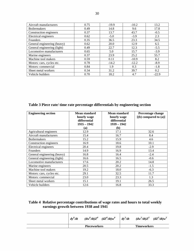
What does a more disaggregated picture reveal? The incidence and growth of
piecework and timework between 1935 and 1942 in fifteen engineering sections –
covering the main areas of wartime activity - are shown in Table 2. In twelve of the
sections, positive growth in the proportions of pieceworkers to timeworkers occurred
between 1935 and 1942. Of the twelve, three sections – construction engineering,
locomotive manufacture and sheet metal working – displayed especially steep growths in
the proportions of pieceworkers during the early war years. Extending the period from
1935 to 1951, only eight sections achieved a positive growth in the proportions of
pieceworkers. Certainly in construction engineering, general engineering (heavy and
light), locomotive manufacture, sheet metal working and vehicle building major relative
growth was decidedly a war-related phenomenon. By contrast, in aircraft and car
manufacture, sizeable reductions in the incidence of pieceworking occurred during the
war affected years. Note, however, that both of these sections displayed well above
average proportions of pieceworkers over the entire period.
As suggested in Section 3, deskilling and the growth of piecework went hand in
hand. Sheet metal working provides an especially well documented example.15 Strong
piecework growth in this section16 occurred for three principal reasons. First, technical
change facilitated deskilling. Skilled manual processes in sheet metal working, involving
hand and bench tools, had been increasingly replaced by power presses and automatic
15 Sheet metal working was a vital war-related production activity, with essential applications in aircraft, vehicle and ship building. It concerns the engineering of thinner varieties of metal plate. A sheet metal worker cuts out, bends, and beats metal into shape (panel beating) and also laps, rivets and solders joints. Deskilling in sheet metal work in the early war years involved protracted collective bargaining discussions involving unions, employers and government (see Inman, 1957, pp. 60/1). 16 The proportion of pieceworkers in sheet metal working climbed from 11 percent of total employment in 1938 to 60 percent in 1942.
18
tools. The latter could be operated by less skilled labour. Even where traditional skilled
work was retained – for example, in the use of free hand methods in the shaping of metal
– associated operations (like drilling and riveting) could be carried out by semi-skilled
workers. Those engaged in pressing, drilling and riveting performed relatively narrow
and repetitive tasks that were suited to piece rated systems. Second, the greater labour
heterogeity linked to deskilling increased the worth of measuring and rewarding
individual value added. Third, sheet metal working was especially important in aircraft
manufacture, centred in the Midlands. There were extremely high labour shortages in
this region. Piece rates had to be settled on a job by job basis. High demand, rapid
technical change and process diversity combined to drive up piece rates to very high
levels and this helped employers to retain their most productive workers as well as
encouraging mobility from outside industries (see Section 7).
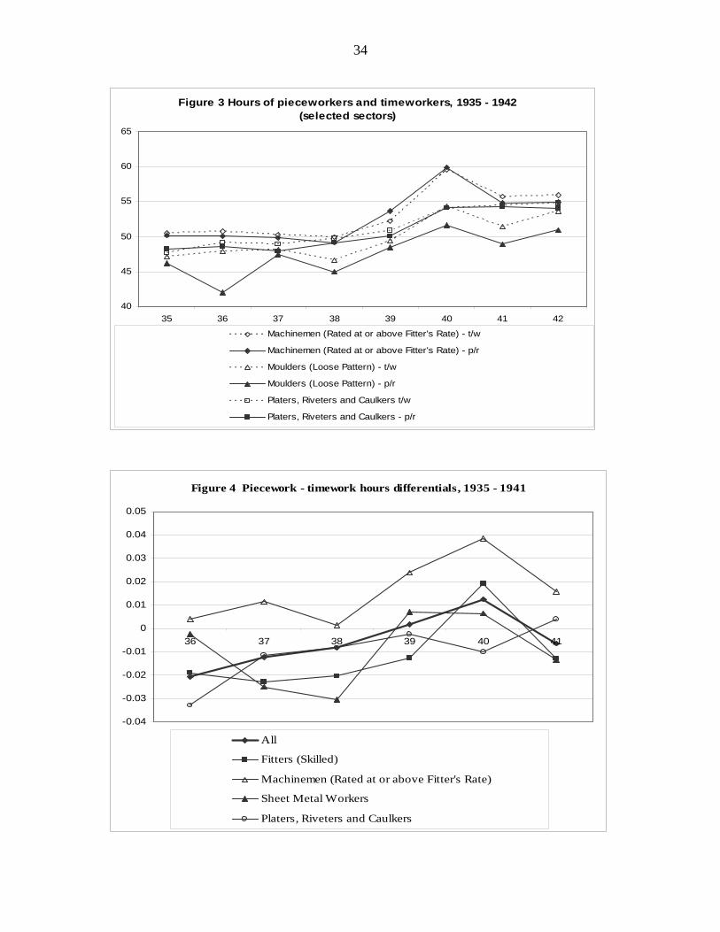
Hours
What about labour expansion on firms’ intensive margins, as represented by
average weekly hours of work? As would be expected, average weekly hours grew
dramatically during the early part of the war. The standard workweek in engineering
between 1919 and 1946 was 47 hours. The year of peak industrial activity was 1940.
Average hours in sheet metal working, aircraft manufacture, heavy general engineering
and marine engineering – all vital wartime engineering sections - was 59 hours in 1940,
representing 12 hours of average weekly overtime. 17 A representative pattern of weekly
hours between 1935 and 1942 is shown in Figure 3 for three occupations of piece rated
17 Contrasting with average weekly hours of between 44 and 46 in 1931, the depth of the Great Depression.

19
workers (p/r) and time rated workers (t/w) averaged across sections. Again, the peak year
is 1940, with skilled machinemen averaging 60 hours per week.
What happened to the hours’ growth of pieceworkers relative to timeworkers?
The following regression was undertaken with respect to occupation i in engineering
section s at time t
(7) isttsi
Tist
Pist edddhh +++=− loglog
where hP (hT ) is the weekly hours of pieceworkers (timeworkers), di are occupational
intercepts, ds are section intercepts, dt are time intercepts and eist is an error term. There
are seven occupation groups18, twenty seven sections19, and seven years (from 1935 to
194120).
e
Estimation of equation (7) is
estimated for single key occupation
variable in (7) was regressed on eng
the estimated time dummies from (
with the time dummies of the four s 18 Skilled fitters, labourers, machinemen (rrate), moulders (loose pattern), platers/rive 19 Agricultural engineers, aircraft manufacengineers, coppersmiths, electrical engineegeneral engineers (light), instrument makemanufacturers, machine tool makers, marinscale/beam etc. makers, sheet metal workemachinery makers, vehicle builders, misce 20 The year 1942 is omitted because availa
Figure 3 and 4 her
based on 840 observations. A variant of (7) was also
s. For each selected occupation, the dependent
ineering sections and time dummies. Figure 4 plots
) from the total regression of equation (7) together
elected occupations. In general, the results clearly
td̂
ated at or above fitter’s rate), machinemen (rated below fitter’s ters/caulkers, sheet metal workers.
turers, allied trades, boilermakers, brassfounders, construction rs, founders, gas meter makers, general engineers (heavy), rs, lamp manufacturers, lift manufacturers, locomotive e engineers, motors (cars, cycles etc.), motors (commercial),
rs, tank and gasholder makers, telephone manufacturers, textile llaneous.
ble data are far less comprehensive for that year.
20
indicate that the hours of pieceworkers rose relative to timeworkers, especially during the
frenetic production period from 1938 to 1940.
6 Wage differentials, relative earnings growth, and labour heterogeneity
Wage differentials
In common with general findings in the literature, the wages of pieceworkers
exceed timeworkers in our data. Based on 15 engineering sections and covering the most
important wartime engineering activities, Table 3 shows that between 1935 and 1942, the
sectional wage differentials varied between 12 and 30 percent. Additionally, the table
reveals that for ten of these sections, the early war years marked a rise in the differential
compared to the period as a whole. The increase is substantial (in excess of 25 percent)
in agricultural engineering, sheet metal working and vehicle building.
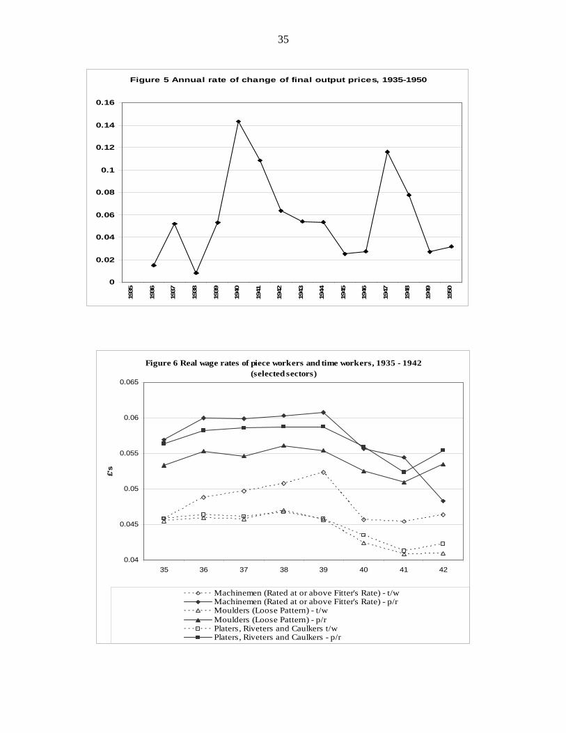
A critical consideration in the analysis of real wages is the steep price inflation
that occurred between 1938 and 1940. From Figure 5, it can be seen that the annual rate
of change of final output prices increased more than 7- fold during these two years. Both
pieceworkers’ and timeworkers’ real hourly wage rates fell during this period, as
illustrated for selected occupations (averaged across sections) in Figure 6. However,
given steep contemporaneous rises in weekly hours (see Figure 3), there were net
increases in real weekly earnings (i.e. real hourly rates times average weekly hours) as
revealed in Figure 7. Note also that, consistent with Table 3, wage rates and earnings of
pieceworkers were above respective wages of timeworkers.
e
Figures 5, 6 and 7 her
21
I now consider piecework-timework wage differentials in more detail. Replacing hours
as dependent variable in equation (7) with and estimating with the same
occupations and sections produces the results shown in Figure 8. At the outset of war in
1939 there was a clear widening of the piece rate/time rate differentials from the sectoral
estimates. The gap was especially pronounced in sheet metal working.
Tist
Pist ww loglog −
e
Wages and hours
Further insights into th
taking advantage of the relativ
overtime pay that prevailed in
overtime was remunerated at 1
timeworkers, weekly earnings
expressed
(8) yT = wT.ZT
where ZT = 47 + max{(hT – 47 Differentiating with respect to
(9) T
TTT
wdt
dZZdt
dwdt
dy+=
Figure 8 her
e relative roles of wage rates and hours can be obtained by
ely simple rules relating to standard weekly hours and
the industry. The standard workweek was 47 hours while
.5 times the standard hourly rate. Illustrating for
yT involved two variables and two constants, and may be
), 0} × 1.5.
time gives
T .
22
The rules with respect to maximum standard hours and overtime premium pay also
applied to pieceworkers and so the same decomposition can be carried out with respect to
pieceworkers’ earnings (yP), hourly wages (wP), and hours (ZP).
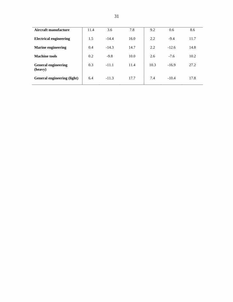
For given maximum standard weekly hours and overtime premium, weekly
earnings can increase for two reasons. First a rise in the standard rate increases both
standard earnings and overtime earnings. Second, a rise in weekly hours above 47 leaves
standard earnings constant but increases overtime earnings. Defining wages and hours
expressions at the mid point of the time interval 1938 – 1941, Table 4 contains values of
the expressions in (9) (given as percentages) for six highly strategic sections of
engineering. In all sections and under both payments’ methods, average weekly real
earnings grew (i.e. dyP/dt > 0 and dyT/dt > 0), although only in aircraft manufacture
(pieceworkers and timeworkers) and general engineering (timeworkers) were the growth
rates substantial. Note, however, that increases derived mainly from changes in hours,
i.e. dZP/dt > 0 and dZT/dt > 0: in most cases real wage rates fell (i.e. dwP/dt < 0 and
dwT/dt < 0 - see also Figure 7).
Table 4 here
Wage differententials and labour heterogeneity Deskilling and the related increase in labour heterogeneity would be expected to
lead to an increase in the relative productivity of pieceworkers since it facilitated an
improved ability both to systematize and to monitor productive performance. It is
possible to test this proposition using the added inference that relative productivity gains
would be reflected in piecework-timework wage differentials.
23
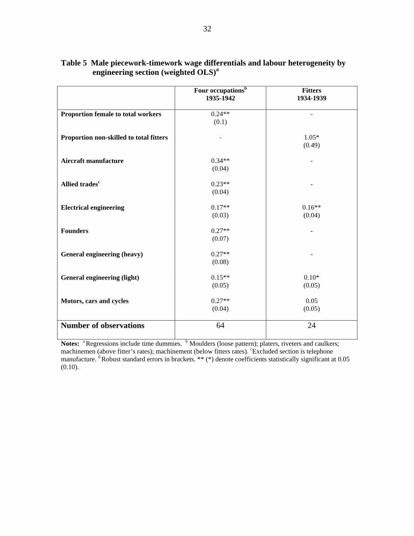
I am able to obtain two measures of labour heterogeneity. The first, and
undoubtedly one of the best measures for the period, is the proportion of women to total
engineering workers. These data are available at a sectional level of aggregation. To
conform, wage data for four male occupation groups (see Table 5) were aggregated to
sectional level. Women were not well represented in all engineering sections and I
confine attention to sections that, based on the four occupations, employed at least 500
women (and at least 500 men) in each and every period from 1935 to 1942. This provided
eight sections in total.21 The second measure relates to one occupational group, male
fitters. Here, for the period 1934 to 1939, I can obtain the proportion of non-skilled
fitters to total fitters. Rearmament commenced in 1935 and issues of skill shortages,
deskilling and greater heterogeneity were also relevant – especially among male workers
– in this earlier period. I considered those sections with at least 500 skilled fitters and at
least 500 unskilled fitters in each and every year, giving four sections in total.
For section s at time t, I estimated the following equation for male piecework-
timework wage differentials
(8) sttsst
Tst
Pst eddbIww +++=− loglog
where I is the index of labour heterogeneity.
Results are shown in Table 5. Both sets of results – i.e. with respect to four
occupational categories in eight sections and fitters in four sections – support the
hypothesis that increased labour heterogeneity was positively associated with the wage
21 The sections are reported in Table 5. Four of these – aircraft manufacture, electrical engineering, heavy general engineering and light general engineering – are sections with high proportions of ‘women doing men’s work’ between 1940 and 1942 (see Hart, 2004, Table 1).
24
differentials. The strength of these associations are underlined by the fact that the two
heterogeneity measures are significant despite the inclusion of time dummies that serve to
take out trend and other systematic time effects.
7 District disaggregation: the importance of the British Midlands The pressures on the engineering industry during the war-affected years were by no
means evenly spread across geographical districts. Before the re-armament period, some
districts had developed engineering and related industries that were to prove essential to
war needs. Leading in this respect was the British Midlands – with its manufacturing
epicentre in Coventy. During the decades preceeding the war, this region had developed
light engineering, vehicle construction and aircraft manufacturing sections. These
activities were essential to war production and, unsurprisingly, related wartime
production – and especially munitions supply – naturally developed alongside. High
earnings attracted significant numbers of immigrant workers from other regions and new
factories were constructed that were geared directly to war provision (Shenfield and
Sargant Florence, 1944-45). Intense inter-firm competition to attract scarce skilled labour
drove up Midlands’ wages well above the average of other areas. Under these
circumstances, and following the aguments in Section 3(b), piece rates offered the best
means of retaining the most productive workers. In fact, there was particularly intense
pressure on piece-rates in the Midlands at this time (Inman, 1957, pp. 320/1).
e
Concentrating on skilled f
relative to (a selection of)
Figures 9, 10 and 11 her
itters, Figures 9 – 11 illustrate the special position of Coventry
other engineering districts. Figure 9 shows that real time rates
25
of pay during the 1935-1942 period were between 10 and 20 percent higher in Coventry
than in London. As for piece rates, Figure 10 reveals that war pressure produced a 30
percent differential between Coventry and the next highest district by 1942, with
exponential growth in rates post 1938. Additional time-series data are available for
skilled fitters allowing us to see, in Figure 11, the piece rate/time rate differentials in a
longer term perspective, from 1927 to 1942. The intense impact of war activity on the
Coventry district is highlighted by an extreme outlying growth in the differential
compared to elsewhere.
8 Conclusions There are six main sets of findings pertaining to male pieceworkers and timeworkers. (a) Piece rates exhibited significant positive demand elasticities in the rearmament years
that preceeded the war in sharp contrast to time rates.
(b) Generally, the proportions of pieceworkers to total workers rose during the war in the
most important wartime sections of the industry from already high levels. From both
employment and wage perspectives, sheet metal working experienced the most
radical shift towards piece-rated work.
(c) While the weekly hours of both timeworkers and pieceworkers grew substantially in
the early war years from already historically high levels, piecework/timework hours
differentials increased.
(d) The importance of hours growth, from the perspectives of both pieceworkers and
timeworkers, is underlined by the fact that during the war real weekly earnings rose
despite real reductions in hourly piece and time rates.

26
(e) Piecework/timework wage differentials widened considerably in the early war years.
The widening wage levels and differentials were especially marked in Coventry, the
centre of aircraft manufacture, vehicle construction and munitions supply and the
most vital engineering district in relation to war production.
(f) Widening piecework-timework wage differentials were significantly associated with
increased labour heterogeneity.
27
References Brown, C. 1990. Firms’ choice of method of pay. Industrial and Labor Relations Review
43 (Special Issue), 165-S – 182-S.
Card, D. 1995. The wage curve: a review. Journal of Economic Literature 33, 785-799.
Cowling, M. 1991. Fixed wages or productivity pay: evidence from 15 EU countries.
Small Business Economics 16, 191-204.
Devereux, P J. 2001. The cyclicality of real wages within employer-employee matches.
Industrial and Labor Relations Review 54: 835-850.
Fama, E F. 1991. Time, salary, and incentive payoffs in labor contracts. Journal of Labor
Economics 9, 25-44.
Feinstein, C H., 1972, National income, expenditure and output of the United Kingdom
1855-1965, Cambridge, Cambridge University Press.
Gibbons, R and K J Murphy. 1992. Optimal incentive contracts in the presence of
career concerns: theory and evidence. Journal of Political Economy 100, 468-505.
Goldin, C. 1986. Monitoring costs, occupational segregation by sex: a historical analysis.
Journal of Labor Economics 4, 1–27.
Hart, R A. 2004. Women doing men’s work and women doing women’s work: female
work and pay in British wartime engineering. Department of Economics,
University of Stirling (mimeo).
Hart, R A and D I MacKay. 1975. Engineering earnings in Britain, 1914-68, Journal of
the Royal Statistical Society (Series A) 138, 32-50.
Heywood, J S, W S Seibert and X Wei. 1997. Payments by results systems: British
evidence. British Journal of Industrial Relations 35, 1-22.
Inman, P. 1957. Labour in the munitions industries. London: HMSO.
Joint Committee of the Institution of Production Engineers and the Institute of Cost
and Works Accountants. 1949. Interim report on meausurement of productivity.
Knowles, KG J C and T P. Hill. 1954. The structure of engineering earnings. Bulletin
of the Oxford University Institute of Statistics 16, 272-328.
Knowles, K G J C and D J. Robertson. 1951a. Some notes on engineering earnings,
Bulletin of the Oxford Institute of Statistics 13, 223-228.
28
Knowles, K G J C and D J Robertson. 1951b. Earnings in engineering, 1926-1948.
Bulletin of the Oxford Institute of Statistics 13, 179-200.
Lazear, E P. 1986. Salaries and piece rates, Journal of Business 59, 405-431.
Lazear, E P. 2001. Performance pay and productivity. American Economic Review 90,
1346 – 1361.
Marsh, A. 1965. Industrial relations in engineering. London, Pergamon Press.
MacLeod, W B and J M Malcomson. 1989. Implicit contracts, incentive compatibility,
and involuntary unemployment. Econometrica 57, 447-480.
Ministry of Labour and National Service. 1947. Report for the years 1939 – 1946.
London: HMSO.
Moulton, B R. 1986. Random group effects and the precision of regression estimates.
Journal of Econometrics 32: 385-397.
Paarsch, H J and B Shearer. 2000. Piece rates, fixed wages, and incentive effects:
statistical evidence from payroll records. International Economic Review 41, 59 –
92.
Parker, R A C. 1981. British rearmament 1936-9: Treasury, trade unions and skilled
labour. English Historical Review 96, 306-43.
Pencavel, J. 1977. Work effort, on-the-job screening, and alternative methods of
remuneration, Research in Labor Economics 1, 225-258.
Shenfield, A and P Sargent Florence. 1944-1945. The economies and diseconomies of
industrial concentration: the wartime experience of Coventry. Review of
Economic Studies 12, 79-99.
Seiler, E. 1984. Piece rate vs. time rate: the effect of incentives on earnings, Review of
Economics and Statistics 66, 363-376.
Solon, G, R Barsky, and J A. Parker. 1994. Measuring the cyclicality of real wages:
how important is composition bias? Quarterly Journal of Economics 109, 1-26.
29
Table 1 Effects of a change in the unemployment rate on changes in the log real hourly standard wages of pieceworkers and timeworkers
Fifteen occupations, 1935-1938 Skilled fitters, 1926-1938
Piece-rate workers Time-rate workers Piece-rate
workers
Time-rate
workers
∆urt -0.49*
(0.24)
0.02
(0.19)
-0.35**
(0.14)
-0.01
(0.05)
urt -0.68
(0.38)
0.08
(0.29)
-0.39**
(0.19)
-0.02
(0.06)
urt-1 0.41
(0.22)
0.02
(0.16)
0.33**
(0.14)
0.002
(0.05)
Observations 59 59
204 180
Notes: The first two results columns refer to the second-stage estimates of equation (6). Associated first-stage estimates – i.e. equation (5) – are based on 546 observations. Estimates in the last two columns are based in equation (4). Figures in parenthesis are robust standard errors. ** (*) denote coefficients statistically significant at 0.05 (0.10). The dependent variables are multiplied by 100 so that the estimated unemployment coefficients represent percentage changes in the real wage for a one point increase in the unemployment rate.
Table 2 Relative incidence and growth of piecework by engineering section, 1935- 1951 Engineering section Mean
proportion of pieceworkers 1935 – 1942
Percentage change in proportion 1935-1942
Percentage change in proportion 1939 - 1942
Percentage change in proportion 1935 – 1951
Agricultural engineers 0.61 7.9 2.9 -11.8
30
Aircraft manufacturers 0.75 -19.9 -10.2 13.2 Boilermakers 0.49 14.8 9.6 17.8 Construction engineers 0.37 13.7 43.7 -0.5 Electrical engineers 0.62 -5.0 -3.9 2.3 Founders 0.35 36.5 23.3 34.5 General engineering (heavy) 0.62 20.0 12.9 6.5 General engineering (light) 0.49 22.7 12.3 -5.5 Locomotive manufacturers 0.65 5.0 15.7 -3.9 Marine engineers 0.37 23.9 25.2 55.7 Machine tool makers 0.59 0.11 -10.9 8.2 Motors: cars, cycles etc. 0.78 -14.2 -12.2 -8.9 Motors: commercial 0.84 1.9 0.3 -1.8 Sheet metal workers 0.34 31.2 39.7 0.2 Vehicle builders 0.70 18.2 4.7 -22.9
Table 3 Piece rate/ time rate percentage differentials by engineering section Engineering section Mean standard
hourly wage differential 1935 – 1942
(a)
Mean standard hourly wage differential 1939 – 1942
(b)
Percentage change [(b) compared to (a)]
Agricultural engineers 12.9 17.1 32.6 Aircraft manufacturers 15.4 16.7 8.4 Boilermakers 15.2 15.9 4.6 Construction engineers 16.9 18.6 10.1 Electrical engineers 20.4 19.8 -2.9 Founders 14.9 16.9 13.4 General engineering (heavy) 16.8 16.4 -2.4 General engineering (light) 16.6 16.5 -0.6 Locomotive manufacturers 17.6 20.2 14.8 Marine engineers 20.5 20.2 -1.5 Machine tool makers 19.2 18.0 -6.3 Motors: cars, cycles etc. 29.1 32.5 11.7 Motors: commercial 23.0 23.3 1.3 Sheet metal workers 15.1 19.1 26.5 Vehicle builders 12.6 16.8 33.3
Table 4 Relative percentage contributions of wage rates and hours to total weekly
earnings growth between 1938 and 1941
dyP/dt
(dwP/dt)ZP
(dZP/dt)wP
dyT/dt
(dwT/dt)ZT
(dZT/dt)wT
Pieceworkers Timeworkers
31
Aircraft manufacture
11.4 3.6 7.8 9.2 0.6 8.6
Electrical engineering 1.5 -14.4 16.0 2.2 -9.4 11.7 Marine engineering
0.4 -14.3 14.7 2.2 -12.6 14.8
Machine tools
0.2 -9.8 10.0 2.6 -7.6 10.2
General engineering (heavy)
0.3 -11.1 11.4 10.3 -16.9 27.2
General engineering (light)
6.4 17.7 7.4 17.8 -11.3 -10.4
32
Table 5 Male piecework-timework wage differentials and labour heterogeneity by
engineering section (weighted OLS)a
Four occupationsb
1935-1942 Fitters
1934-1939
Proportion female to total workers
0.24** (0.1)
-
Proportion non-skilled to total fitters
-
1.05* (0.49)
Aircraft manufacture
0.34** (0.04)
-
Allied tradesc
0.23** (0.04)
-
Electrical engineering
0.17** (0.03)
0.16** (0.04)
Founders
0.27** (0.07)
-
General engineering (heavy)
0.27** (0.08)
-
General engineering (light)
0.15** (0.05)
0.10* (0.05)
Motors, cars and cycles
0.27** (0.04)
0.05 (0.05)
Number of observations
64 24
Notes: a Regressions include time dummies. b Moulders (loose pattern); platers, riveters and caulkers; machinemen (above fitter’s rates); machinement (below fitters rates). cExcluded section is telephone manufacture. d Robust standard errors in brackets. ** (*) denote coefficients statistically significant at 0.05 (0.10).
33
Figure 1 Annual percentage change in real industrial production 1935-1938 (selected manufacturing industries)
-10
-5
0
5
10
15
20
1935 1936 1937 1938
Perc
ent
Engineering Total manufacturing ChemicalsBuilding Textiles
Source: Feinstein (1972)
Figure 2 Industrial and Armed Forces Employment 1938-1945 (thousands)
0
1000
2000
3000
4000
5000
6000
1938 1939 1940 1941 1942 1943 1944 1945engineering, metals, vehicles and shipbuilding AgricultureChemicals TextilesBuilding TransportDistributive FinancialArmed Forces
34
Figure 3 Hours of pieceworkers and timeworkers, 1935 - 1942 (selected sectors)
40
45
50
55
60
65
35 36 37 38 39 40 41 42
Machinemen (Rated at or above Fitter's Rate) - t/w
Machinemen (Rated at or above Fitter's Rate) - p/r
Moulders (Loose Pattern) - t/w
Moulders (Loose Pattern) - p/r
Platers, Riveters and Caulkers t/w
Platers, Riveters and Caulkers - p/r
Figure 4 Piecework - timework hours differentials, 1935 - 1941
-0.04
-0.03
-0.02
-0.01
0
0.01
0.02
0.03
0.04
0.05
36 37 38 39 40 41
All
Fitters (Skilled)
Machinemen (Rated at or above Fitter's Rate)
Sheet Metal Workers
Platers, Riveters and Caulkers
35
Figure 5 Annual rate of change of final output prices, 1935-1950
0
0.02
0.04
0.06
0.08
0.1
0.12
0.14
0.16
1935
1936
1937
1938
1939
1940
1941
1942
1943
1944
1945
1946
1947
1948
1949
1950
Figure 6 Real wage rates of piece workers and time workers, 1935 - 1942 (selected sectors)
0.04
0.045
0.05
0.055
0.06
0.065
35 36 37 38 39 40 41 42
£'s
Machinemen (Rated at or above Fitter's Rate) - t/wMachinemen (Rated at or above Fitter's Rate) - p/rMoulders (Loose Pattern) - t/wMoulders (Loose Pattern) - p/rPlaters, Riveters and Caulkers t/wPlaters, Riveters and Caulkers - p/r
36
Figure 7 Real weekly earnings of pieceworkers and timeworkers, 1935-1942
2
2.2
2.4
2.6
2.8
3
3.2
3.4
3.6
3.8
35 36 37 38 39 40 41 42
£'s
Machinemen (Rated at or above Fitter's Rate) - t/wMachinemen (Rated at or above Fitter's Rate) - p/rMoulders (Loose Pattern) - t/wMoulders (Loose Pattern) - p/rPlaters, Riveters and Caulkers t/wPlaters, Riveters and Caulkers - p/r
Figure 8 Piecework -timework wage rate differentials, 1935-1941
-0.02
0
0.02
0.04
0.06
0.08
0.1
0.12
36 37 38 39 40 41
All
Fitters (Skilled)
Machinemen (Rated at or above Fitter's Rate)
Moulders (Loose Pattern)
Platers, Riveters and Caulkers
Sheet Metal Workers
37
Figure 9 Real wages of timeworkers (skilled fitters), 1935 - 1942 (selected EEF districts)
0.04
0.042
0.044
0.046
0.048
0.05
0.052
0.054
0.056
0.058
0.06
35 36 37 38 39 40 41 42
Coventry London Liverpool Nth Est Coast Sheffield
Figure 10 Real wages of pieceworkers (skilled fitters) 1935 - 1942 (selected EEF districts)
0.045
0.05
0.055
0.06
0.065
0.07
0.075
0.08
0.085
35 36 37 38 39 40 41 42
Coventry London Liverpool Nth Est Coast Sheffield
38
Figure 11 Piece rate/time rate differentials of skilled fitters, 1927-1942 (selected districts)
0
0.1
0.2
0.3
0.4
0.5
0.6
1927
1928
1929
1930
1931
1932
1933
1934
1935
1936
1937
1938
1939
1940
1941
1942
Coventry London Sheffield N.E. coast