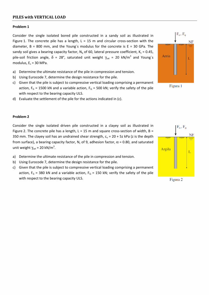
PILES with VERTICAL LOAD

Problem 1

Consider the single isolated bored pile constructed in a sandy soil as illustrated in

Figure 1. The concrete pile has a length, L = 15 m and circular cross-section with the

diameter, B = 800 mm, and the Young´s modulus for the concrete is E = 30 GPa. The

sandy soil gives a bearing capacity factor, Nq of 60, lateral pressure coefficient, Ks = 0.45,

pile-soil friction angle, δ = 28°, saturated unit weight γsat = 20 kN/m3 and Young´s

modulus, Es = 30 MPa.

a) Determine the ultimate resistance of the pile in compression and tension.

b) Using Eurocode 7, determine the design resistance for the pile.

c) Given that the pile is subject to compressive vertical loading comprising a permanent

action, FG = 1500 kN and a variable action, FQ = 500 kN; verify the safety of the pile

with respect to the bearing capacity ULS.

d) Evaluate the settlement of the pile for the actions indicated in (c).

Problem 2

Consider the single isolated driven pile constructed in a clayey soil as illustrated in

Figure 2. The concrete pile has a length, L = 15 m and square cross-section of width, B =

350 mm. The clayey soil has an undrained shear strength, cu = 20 + 5z kPa (z is the depth

from surface), a bearing capacity factor, Nc of 9, adhesion factor, α = 0.80, and saturated

unit weight γsat = 20 kN/m3.

a) Determine the ultimate resistance of the pile in compression and tension.

b) Using Eurocode 7, determine the design resistance for the pile.

c) Given that the pile is subject to compressive vertical loading comprising a permanent

action, FG = 380 kN and a variable action, FQ = 150 kN; verify the safety of the pile

with respect to the bearing capacity ULS.

Problem 3

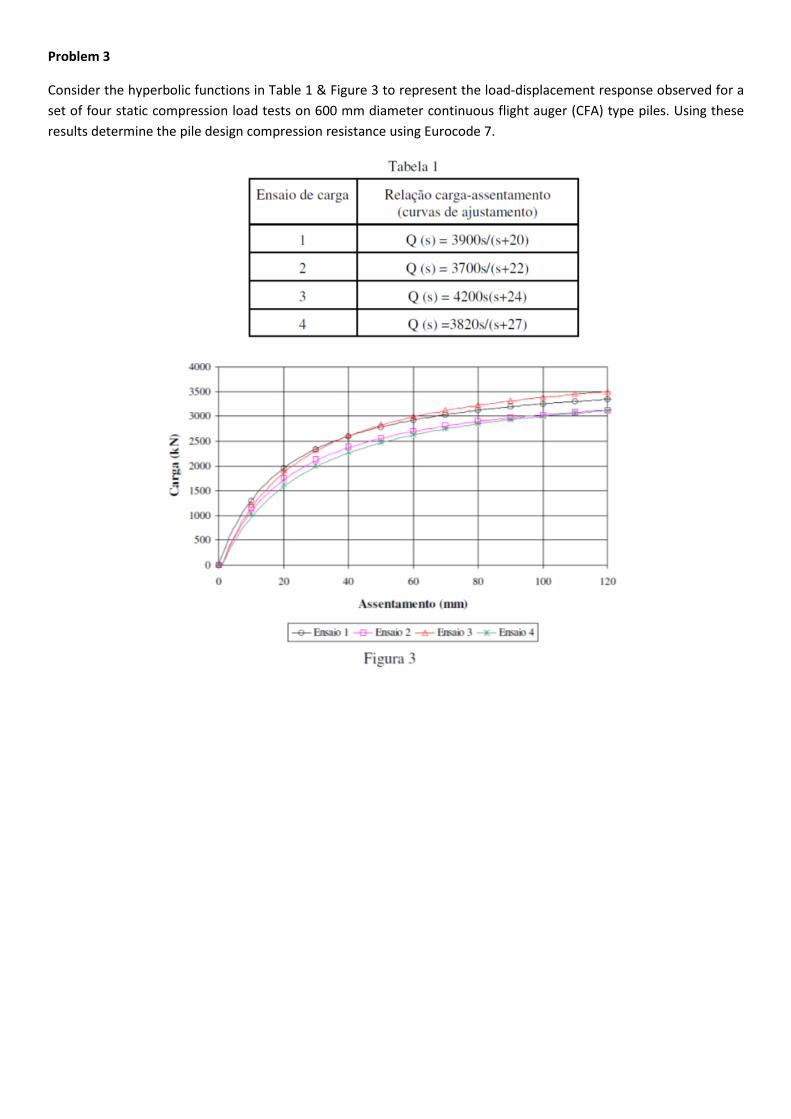
Consider the hyperbolic functions in Table 1 & Figure 3 to represent the load-displacement response observed for a

set of four static compression load tests on 600 mm diameter continuous flight auger (CFA) type piles. Using these

results determine the pile design compression resistance using Eurocode 7.

Problem 4

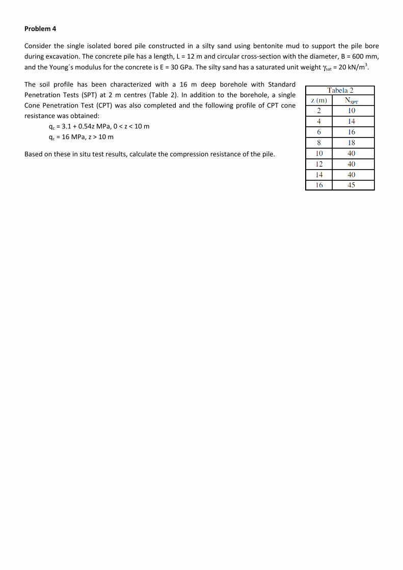
Consider the single isolated bored pile constructed in a silty sand using bentonite mud to support the pile bore

during excavation. The concrete pile has a length, L = 12 m and circular cross-section with the diameter, B = 600 mm,

and the Young´s modulus for the concrete is E = 30 GPa. The silty sand has a saturated unit weight γsat = 20 kN/m3.

The soil profile has been characterized with a 16 m deep borehole with Standard

Penetration Tests (SPT) at 2 m centres (Table 2). In addition to the borehole, a single

Cone Penetration Test (CPT) was also completed and the following profile of CPT cone

resistance was obtained:

qc = 3.1 + 0.54z MPa, 0 < z < 10 m

qc = 16 MPa, z > 10 m

Based on these in situ test results, calculate the compression resistance of the pile.

Formulas

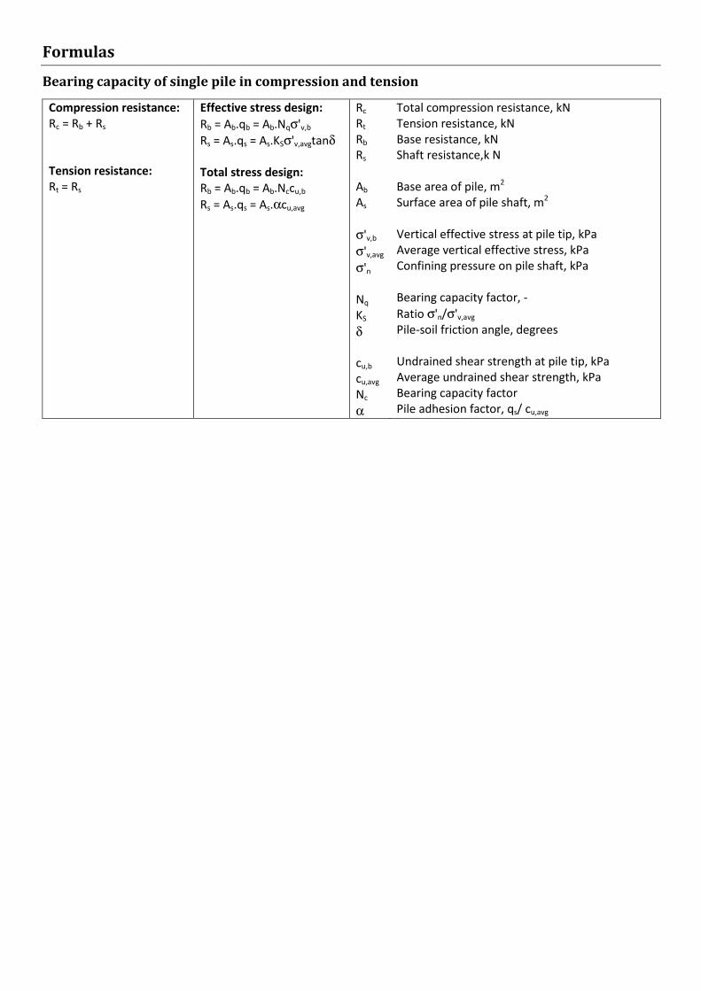
Bearing capacity of single pile in compression and tension

Compression resistance:

Rc = Rb + Rs

Tension resistance:

Rt = Rs

Effective stress design:

Rb = Ab.qb = Ab.Nqσ'v,b

Rs = As.qs = As.KSσ'v,avgtanδ

Total stress design:

Rb = Ab.qb = Ab.Nccu,b

Rs = As.qs = As.αcu,avg

Rc

Rt

Rb

Rs

Ab

As

σ'v,b

σ'v,avg

σ'n

Nq

KS

δ cu,b

cu,avg

Nc

α

Total compression resistance, kN

Tension resistance, kN

Base resistance, kN

Shaft resistance,k N

Base area of pile, m2

Surface area of pile shaft, m2

Vertical effective stress at pile tip, kPa

Average vertical effective stress, kPa

Confining pressure on pile shaft, kPa

Bearing capacity factor, -

Ratio σ'n/σ'v,avg

Pile-soil friction angle, degrees

Undrained shear strength at pile tip, kPa

Average undrained shear strength, kPa

Bearing capacity factor

Pile adhesion factor, qs/ cu,avg

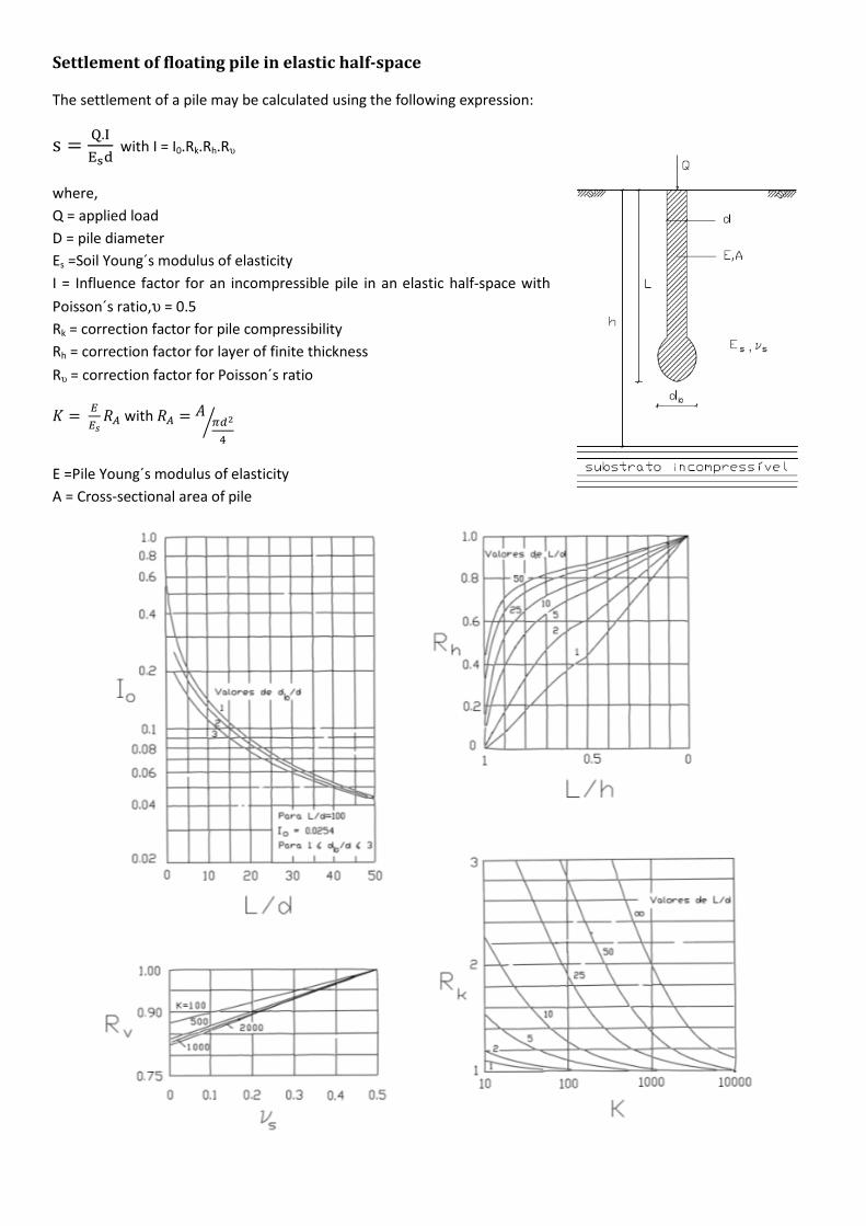
Settlement of floating pile in elastic half-space

The settlement of a pile may be calculated using the following expression:

s = �.���� with I = I0.Rk.Rh.Rυ

where,

Q = applied load

D = pile diameter

Es =Soil Young´s modulus of elasticity

I = Influence factor for an incompressible pile in an elastic half-space with

Poisson´s ratio,υ = 0.5

Rk = correction factor for pile compressibility

Rh = correction factor for layer of finite thickness

Rυ = correction factor for Poisson´s ratio

= ��� � with � = � �����

E =Pile Young´s modulus of elasticity

A = Cross-sectional area of pile

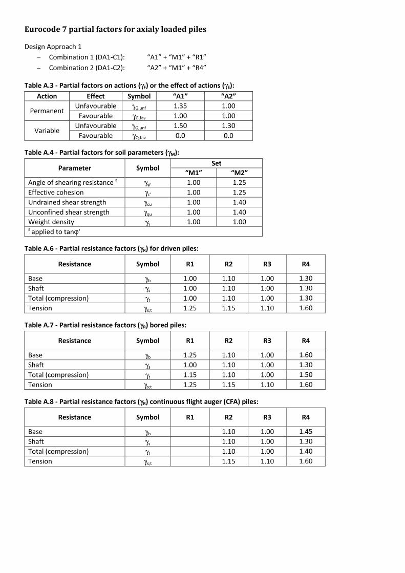
Eurocode 7 partial factors for axialy loaded piles

Design Approach 1

– Combination 1 (DA1-C1): “A1” + “M1” + “R1”

– Combination 2 (DA1-C2): “A2” + “M1” + “R4”

Table A.3 - Partial factors on actions (γF) or the effect of actions (γE):

Action Effect Symbol “A1” “A2”

Permanent Unfavourable γG,unf 1.35 1.00

Favourable γG,fav 1.00 1.00

Variable Unfavourable γQ,unf 1.50 1.30

Favourable γQ,fav 0.0 0.0

Table A.4 - Partial factors for soil parameters (γM):

Parameter Symbol Set

“M1” “M2”

Angle of shearing resistance a γϕ' 1.00 1.25

Effective cohesion γc' 1.00 1.25

Undrained shear strength γcu 1.00 1.40

Unconfined shear strength γqu 1.00 1.40

Weight density γγ 1.00 1.00 a applied to tanϕ'

Table A.6 - Partial resistance factors (γR) for driven piles:

Resistance Symbol R1 R2 R3 R4

Base γb 1.00 1.10 1.00 1.30

Shaft γs 1.00 1.10 1.00 1.30

Total (compression) γt 1.00 1.10 1.00 1.30

Tension γs;t 1.25 1.15 1.10 1.60

Table A.7 - Partial resistance factors (γR) bored piles:

Resistance Symbol R1 R2 R3 R4

Base γb 1.25 1.10 1.00 1.60

Shaft γs 1.00 1.10 1.00 1.30

Total (compression) γt 1.15 1.10 1.00 1.50

Tension γs;t 1.25 1.15 1.10 1.60

Table A.8 - Partial resistance factors (γR) continuous flight auger (CFA) piles:

Resistance Symbol R1 R2 R3 R4

Base γb 1.10 1.00 1.45

Shaft γs 1.10 1.00 1.30

Total (compression) γt 1.10 1.00 1.40

Tension γs;t 1.15 1.10 1.60

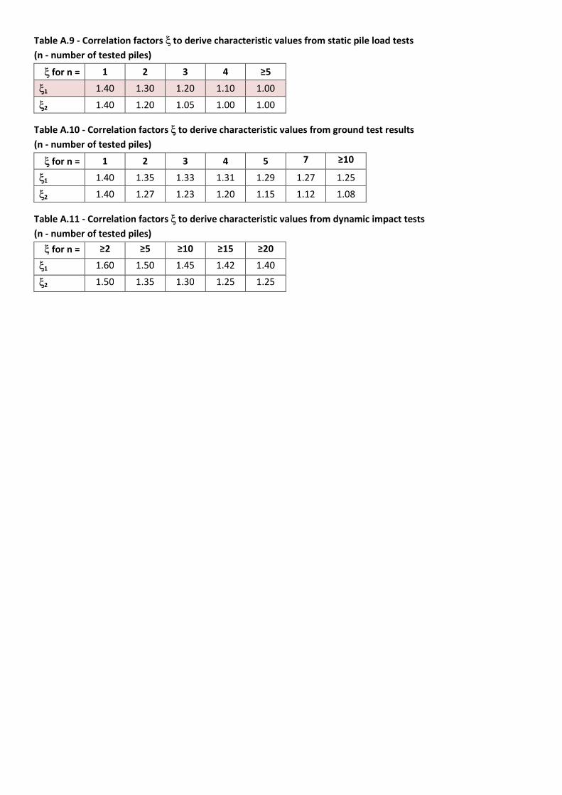
Table A.9 - Correlation factors ξ to derive characteristic values from static pile load tests

(n - number of tested piles)

ξ for n = 1 2 3 4 ≥5

ξ1 1.40 1.30 1.20 1.10 1.00

ξ2 1.40 1.20 1.05 1.00 1.00

Table A.10 - Correlation factors ξ to derive characteristic values from ground test results

(n - number of tested piles)

ξ for n = 1 2 3 4 5 7 ≥10

ξ1 1.40 1.35 1.33 1.31 1.29 1.27 1.25

ξ2 1.40 1.27 1.23 1.20 1.15 1.12 1.08

Table A.11 - Correlation factors ξ to derive characteristic values from dynamic impact tests

(n - number of tested piles)

ξ for n = ≥2 ≥5 ≥10 ≥15 ≥20

ξ1 1.60 1.50 1.45 1.42 1.40

ξ2 1.50 1.35 1.30 1.25 1.25

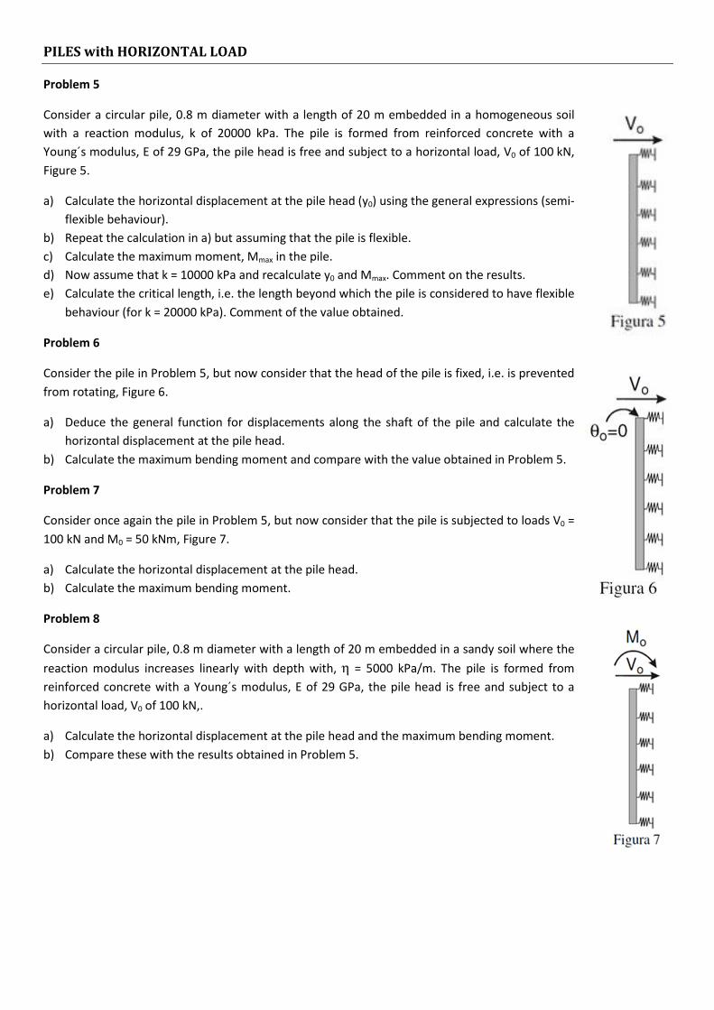
PILES with HORIZONTAL LOAD

Problem 5

Consider a circular pile, 0.8 m diameter with a length of 20 m embedded in a homogeneous soil

with a reaction modulus, k of 20000 kPa. The pile is formed from reinforced concrete with a

Young´s modulus, E of 29 GPa, the pile head is free and subject to a horizontal load, V0 of 100 kN,

Figure 5.

a) Calculate the horizontal displacement at the pile head (y0) using the general expressions (semi-

flexible behaviour).

b) Repeat the calculation in a) but assuming that the pile is flexible.

c) Calculate the maximum moment, Mmax in the pile.

d) Now assume that k = 10000 kPa and recalculate y0 and Mmax. Comment on the results.

e) Calculate the critical length, i.e. the length beyond which the pile is considered to have flexible

behaviour (for k = 20000 kPa). Comment of the value obtained.

Problem 6

Consider the pile in Problem 5, but now consider that the head of the pile is fixed, i.e. is prevented

from rotating, Figure 6.

a) Deduce the general function for displacements along the shaft of the pile and calculate the

horizontal displacement at the pile head.

b) Calculate the maximum bending moment and compare with the value obtained in Problem 5.

Problem 7

Consider once again the pile in Problem 5, but now consider that the pile is subjected to loads V0 =

100 kN and M0 = 50 kNm, Figure 7.

a) Calculate the horizontal displacement at the pile head.

b) Calculate the maximum bending moment.

Problem 8

Consider a circular pile, 0.8 m diameter with a length of 20 m embedded in a sandy soil where the

reaction modulus increases linearly with depth with, η = 5000 kPa/m. The pile is formed from

reinforced concrete with a Young´s modulus, E of 29 GPa, the pile head is free and subject to a

horizontal load, V0 of 100 kN,.

a) Calculate the horizontal displacement at the pile head and the maximum bending moment.

b) Compare these with the results obtained in Problem 5.

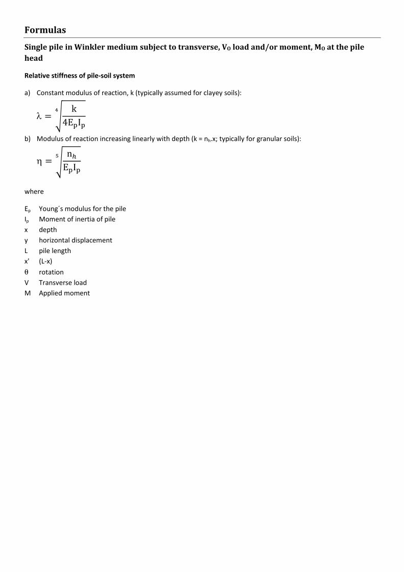
Formulas

Single pile in Winkler medium subject to transverse, VO load and/or moment, MO at the pile

head

Relative stiffness of pile-soil system

a) Constant modulus of reaction, k (typically assumed for clayey soils):

λ = � k4E�I��

b) Modulus of reaction increasing linearly with depth (k = nh.x; typically for granular soils):

η = � n�E�I��

where

Ep Young´s modulus for the pile

Ip Moment of inertia of pile

x depth

y horizontal displacement

L pile length

x' (L-x)

θ rotation

V Transverse load

M Applied moment

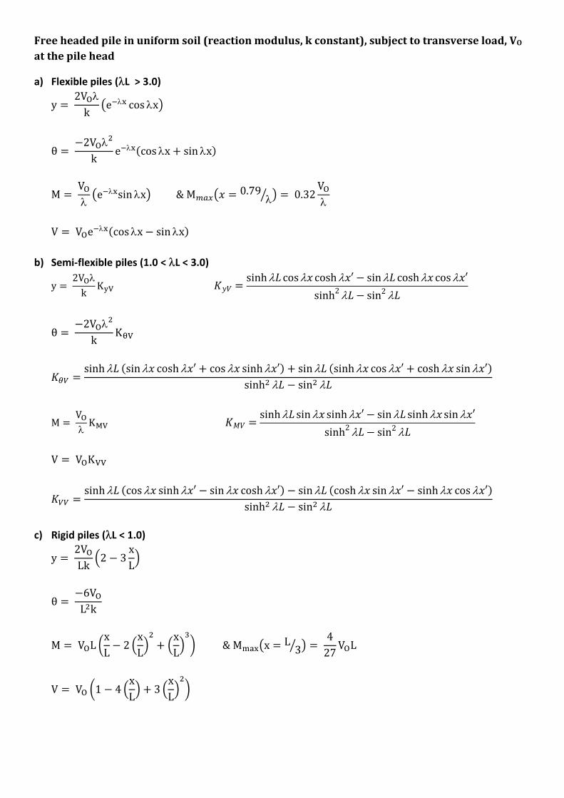
Free headed pile in uniform soil (reaction modulus, k constant), subject to transverse load, VO

at the pile head

a) Flexible piles (λL > 3.0)

y = 2V"λk #e%λ& cosλx*

θ = −2V"λ-k e%λ&.cosλx + sinλx1

M =V"λ#e%λ&sinλx*&M456#7 = 0.79

λ; * = 0.32 V"λ

V = V"e%λ&.cosλx − sinλx1

b) Semi-flexible piles (1.0 < λL < 3.0)

y = 2V"λk K>?@A = sinhλCcosλ7 coshλ7′ − sinλC coshλ7 cosλ7′sinh2 λC − sin2 λC

θ = −2V"λ-k KE?

FG = sinh λC .sinλ7 cosh λ7′ + cos λ7 sinhλ7′1 + sinλC .sinhλ7 cos λ7′ + cosh λ7 sinλ7′1sinh- λC − sin- λC

M =V"λKH?IA = sinhλCsinλ7 sinhλ7′ − sinλCsinhλ7sinλ7′sinh2 λC − sin2 λC

V = V"K??

GG = sinhλC .cosλ7 sinhλ7′ − sin λ7 cosh λ7′1 − sinλC .cosh λ7 sin λ7′ − sinhλ7 cos λ7′1sinh- λC − sin- λC

c) Rigid piles (λL < 1.0)

y = 2V"Lk K2 − 3 xLL

θ = −6V"L-k

M =V"L NxL − 2 KxLL- + KxLLOP &MQR&#x = L 3; * = 427V"L

V = V" N1 − 4 KxLL + 3 KxLL-P

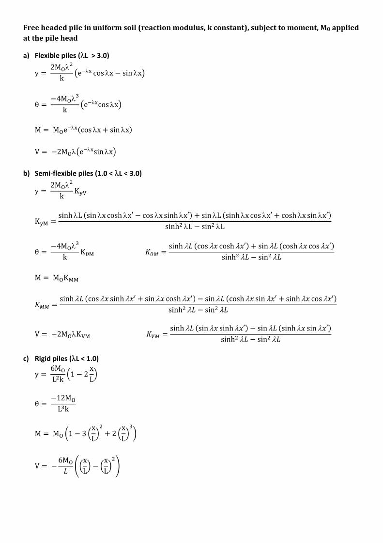
Free headed pile in uniform soil (reaction modulus, k constant), subject to moment, MO applied

at the pile head

a) Flexible piles (λL > 3.0)

y = 2M"λ-k #e%λ& cos λx − sinλx*

θ = −4M"λOk #e%λ&cosλx* M =M"e%λ&.cosλx + sinλx1 V = −2M"λ#e%λ&sinλx*

b) Semi-flexible piles (1.0 < λL < 3.0)

y = 2M"λ-k K>?

K>H = sinhλL .sinλx cosh λx′ − cos λx sinhλx′1 + sinλL .sinhλx cos λx′ + cosh λx sinλx′1sinh- λL − sin- λL

θ = −4M"λOk KEHFT = sinh λC .cos λ7 cosh λ7′1 + sinλC .coshλ7 cos λ7′1sinh- λC − sin- λC

M =M"KHH

TT = sinhλC .cosλ7 sinhλ7′ + sin λ7 cosh λ7′1 − sinλC .coshλ7 sin λ7′ + sinhλ7 cos λ7′1sinh- λC − sin- λC

V = −2M"λK?HGT = sinhλC .sinλ7 sinhλ7′1 − sinλC .sinhλ7 sin λ7′1sinh- λC − sin- λC

c) Rigid piles (λL < 1.0)

y = 6M"L-k K1 − 2 xLL

θ = −12M"LOk

M =M" N1 − 3 KxLL- + 2KxLLOP

V = −6M"C UKxLL − KxLL-V

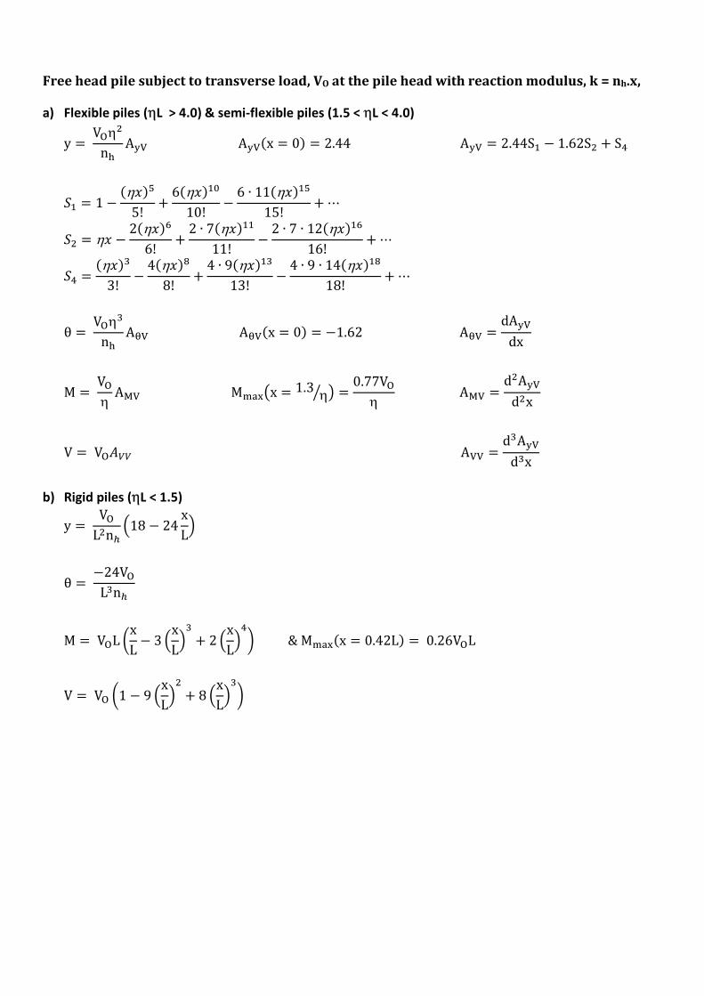
Free head pile subject to transverse load, VO at the pile head with reaction modulus, k = nh.x,

a) Flexible piles (ηL > 4.0) & semi-flexible piles (1.5 < ηL < 4.0)

y = V"η-nW A>?A>?.x = 01 = 2.44A>? = 2.44SZ − 1.62S- + S�

[Z = 1 − .η71\5! + 6.η71Z_10! − 6 ∙ 11.η71Z\15! + ⋯

[- = η7 − 2.η71b6! + 2 ∙ 7.η71ZZ11! − 2 ∙ 7 ∙ 12.η71Zb16! + ⋯

[� = .η71O3! − 4.η71c8! + 4 ∙ 9.η71ZO13! − 4 ∙ 9 ∙ 14.η71Zc18! + ⋯

θ = V"ηOnW AE?AE?.x = 01 = −1.62AE? = dA>?dx

M =V"ηAH?MQR&#x = 1.3

η; * = 0.77V"η

AH? = d-A>?d-x

V = V"�GG A?? = dOA>?dOx

b) Rigid piles (ηL < 1.5)

y = V"L-n� K18 − 24 xLL

θ = −24V"LOn�

M =V"L NxL − 3 KxLLO + 2KxLL�P &MQR&.x = 0.42L1 = 0.26V"L

V = V" N1 − 9 KxLL- + 8KxLLOP

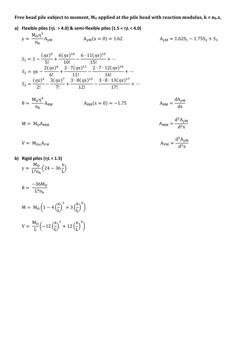
Free head pile subject to moment, MO applied at the pile head with reaction modulus, k = nh.x,

a) Flexible piles (ηL > 4.0) & semi-flexible piles (1.5 < ηL < 4.0)

y = M"ηOnW A>HA>H.x = 01 = 1.62A>H = 1.62SZ − 1.75S- + SO

[Z = 1 − .η71\5! + 6.η71Z_10! − 6 ∙ 11.η71Z\15! + ⋯

[- = η7 − 2.η71b6! + 2 ∙ 7.η71ZZ11! − 2 ∙ 7 ∙ 12.η71Zb16! + ⋯

[O = .η71-2! − 3.η71f7! + 3 ∙ 8.η71Z-12! − 3 ∙ 8 ∙ 13.η71Zf17! + ⋯

θ = M"η�nW AEHAEH.x = 01 = −1.75AEH = dA>Hdx

M =M"AHHAHH = d-A>Hd-x

V = M"η�GTA?H = dOA>HdOx

b) Rigid piles (ηL < 1.5)

y = M"LOn� K24 − 36 xLL

θ = −36M"L�n�

M =M" N1 − 4 KxLLO + 3KxLL�P

V = M"L N−12 KxLL- + 12 KxLLOP

PILE GROUPS

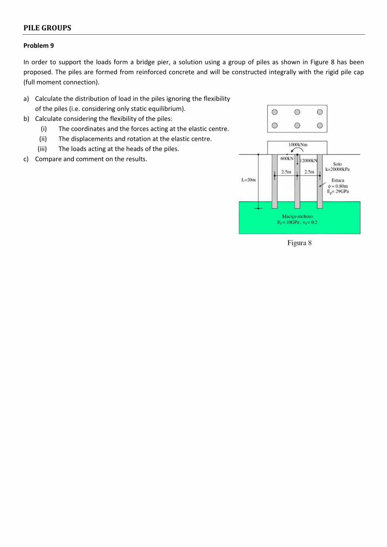
Problem 9

In order to support the loads form a bridge pier, a solution using a group of piles as shown in Figure 8 has been

proposed. The piles are formed from reinforced concrete and will be constructed integrally with the rigid pile cap

(full moment connection).

a) Calculate the distribution of load in the piles ignoring the flexibility

of the piles (i.e. considering only static equilibrium).

b) Calculate considering the flexibility of the piles:

(i) The coordinates and the forces acting at the elastic centre.

(ii) The displacements and rotation at the elastic centre.

(iii) The loads acting at the heads of the piles.

c) Compare and comment on the results.

Formulas

1 - STATIC EQUILIBRIUM METHOD

For the case of a group of “m” number piles can demonstrate that:

gh = ij ± I. 7h∑ 7h-4hmZ

nh = oj

Ih = 0

where

• X, Y & M are the transverse and vertical forces, and moment acting at the base of the pile cap.

• Ti, Ni and Mi are the transverse and vertical forces and moment acting at the head of the i-th pile respectively.

• ei is the distance from the i-th pile to the centre of rotation

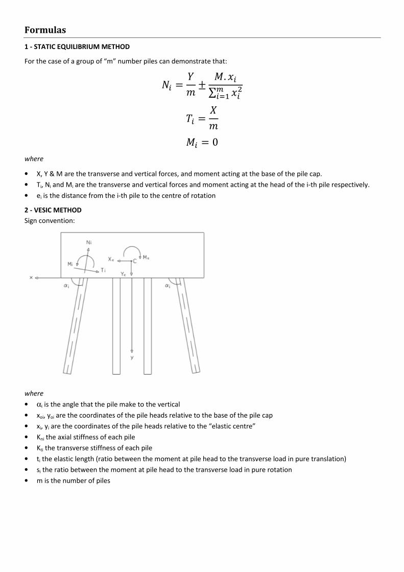
2 - VESIC METHOD

Sign convention:

where

• αi is the angle that the pile make to the vertical

• xoi, yoi are the coordinates of the pile heads relative to the base of the pile cap

• xi, yi are the coordinates of the pile heads relative to the “elastic centre”

• Kni the axial stiffness of each pile

• Kti the transverse stiffness of each pile

• ti the elastic length (ratio between the moment at pile head to the transverse load in pure translation)

• si the ratio between the moment at pile head to the transverse load in pure rotation

• m is the number of piles

For the case of a group of “m” number vertical piles can demonstrate:

(i) Coordinates of the “elastic centre”

7p = ∑ 7qh . rh4hmZ∑ rh4hmZ

@p = ∑ sh . th4hmZ∑ th4hmZ

(ii) Displacements and rotation of the “elastic centre”

uvwxvwyzw { =|}}}}~� ∑ �����; � �

� � ∑ �����; �� � � �′′′; ��

���� ��w�w�w

�

�′′′ =�����x�� + ���.y� + ��1� + ��� N���� − �P ������m�

(iii) Forces in head of each pile

�������� =

|}}}}}~ � ���∑��� −��� x��′′′���∑��� � ��� y� + ���′′′�� ���∑��� � ����� y� + ���′′′ ��

�������w�w�w

�

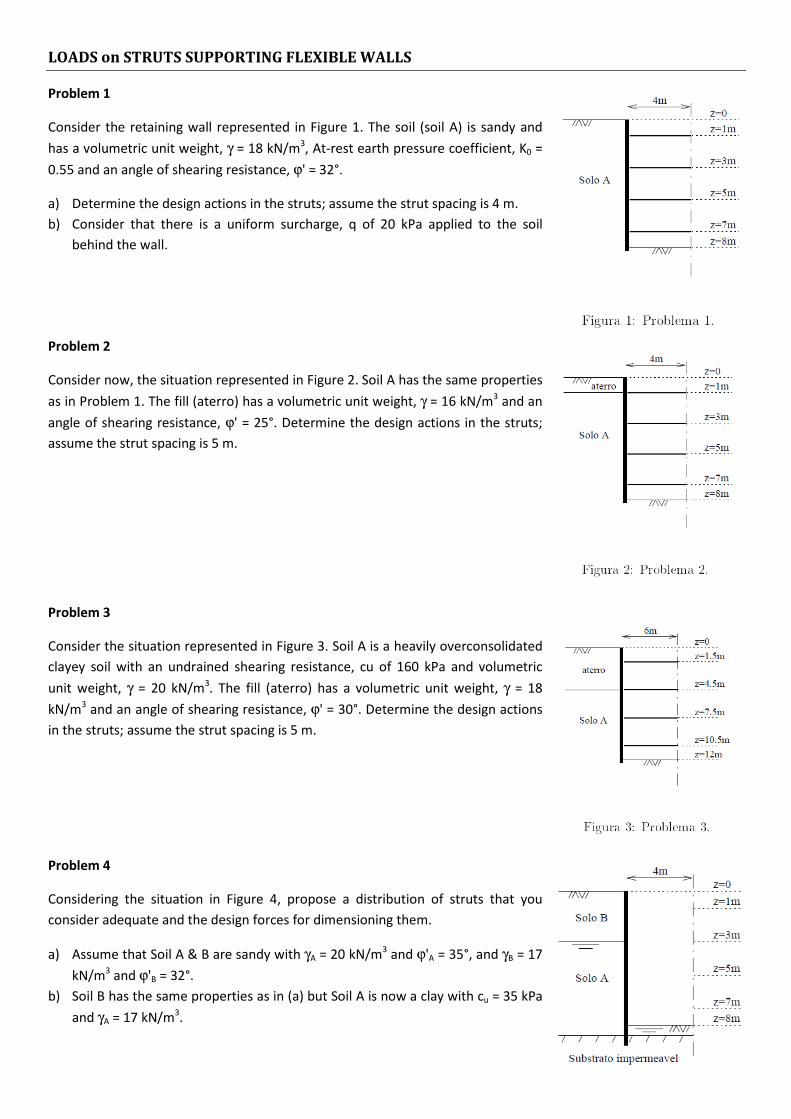
LOADS on STRUTS SUPPORTING FLEXIBLE WALLS

Problem 1

Consider the retaining wall represented in Figure 1. The soil (soil A) is sandy and

has a volumetric unit weight, γ = 18 kN/m3, At-rest earth pressure coefficient, K0 =

0.55 and an angle of shearing resistance, ϕ' = 32°.

a) Determine the design actions in the struts; assume the strut spacing is 4 m.

b) Consider that there is a uniform surcharge, q of 20 kPa applied to the soil

behind the wall.

Problem 2

Consider now, the situation represented in Figure 2. Soil A has the same properties

as in Problem 1. The fill (aterro) has a volumetric unit weight, γ = 16 kN/m3 and an

angle of shearing resistance, ϕ' = 25°. Determine the design actions in the struts;

assume the strut spacing is 5 m.

Problem 3

Consider the situation represented in Figure 3. Soil A is a heavily overconsolidated

clayey soil with an undrained shearing resistance, cu of 160 kPa and volumetric

unit weight, γ = 20 kN/m3. The fill (aterro) has a volumetric unit weight, γ = 18

kN/m3 and an angle of shearing resistance, ϕ' = 30°. Determine the design actions

in the struts; assume the strut spacing is 5 m.

Problem 4

Considering the situation in Figure 4, propose a distribution of struts that you

consider adequate and the design forces for dimensioning them.

a) Assume that Soil A & B are sandy with γA = 20 kN/m3 and ϕ'A = 35°, and γB = 17

kN/m3 and ϕ'B = 32°.

b) Soil B has the same properties as in (a) but Soil A is now a clay with cu = 35 kPa

and γA = 17 kN/m3.

COMPACTION

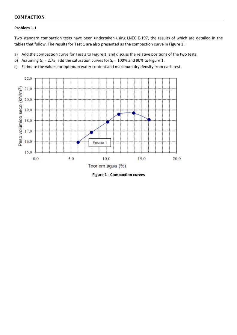
Problem 1.1

Two standard compaction tests have been undertaken using LNEC E-197, the results of which are detailed in the

tables that follow. The results for Test 1 are also presented as the compaction curve in Figure 1 .

a) Add the compaction curve for Test 2 to Figure 1, and discuss the relative positions of the two tests.

b) Assuming Gs = 2.75, add the saturation curves for Sr = 100% and 90% to Figure 1.

c) Estimate the values for optimum water content and maximum dry density from each test.

Figure 1 - Compaction curves

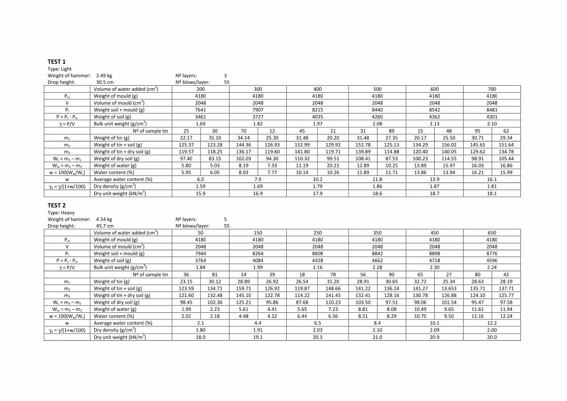
TEST 1

Type: Light

Weight of hammer: 2.49 kg Nº layers: 3

Drop height: 30.5 cm Nº blows/layer: 55

Volume of water added (cm3) 200 300 400 500 600 700

Pm Weight of mould (g) 4180 4180 4180 4180 4180 4180

V Volume of mould (cm3) 2048 2048 2048 2048 2048 2048

Pt Weight soil + mould (g) 7641 7907 8215 8440 8542 8481

P = Pt - Pm Weight of soil (g) 3461 3727 4035 4260 4362 4301

γ = P/V Bulk unit weight (g/cm3) 1.69 1.82 1.97 2.08 2.13 2.10

Nº of sample tin 25 30 70 12 45 21 31 89 15 48 95 62

m1 Weight of tin (g) 22.17 35.10 34.14 25.30 31.48 20.20 31.48 27.35 20.17 25.50 30.71 29.34

m2 Weight of tin + soil (g) 125.37 123.28 144.36 126.93 152.99 129.92 152.78 125.13 134.29 156.02 145.65 151.64

m3 Weight of tin + dry soil (g) 119.57 118.25 136.17 119.60 141.80 119.71 139.89 114.88 120.40 140.05 129.62 134.78

Ws = m3 – m1 Weight of dry soil (g) 97.40 83.15 102.03 94.30 110.32 99.51 108.41 87.53 100.23 114.55 98.91 105.44

Ww = m2 – m3 Weight of water (g) 5.80 5.03 8.19 7.33 11.19 20.21 12.89 10.25 13.89 15.97 16.03 16.86

w = 100(Ww/Ws) Water content (%) 5.95 6.05 8.03 7.77 10.14 10.26 11.89 11.71 13.86 13.94 16.21 15.99

w Average water content (%) 6.0 7.9 10.2 11.8 13.9 16.1

γd = γ/(1+w/100) Dry density (g/cm3) 1.59 1.69 1.79 1.86 1.87 1.81

Dry unit weight (kN/m3) 15.9 16.9 17.9 18.6 18.7 18.1

TEST 2

Type: Heavy

Weight of hammer: 4.54 kg Nº layers: 5

Drop height: 45.7 cm Nº blows/layer: 55

Volume of water added (cm3) 50 150 250 350 450 650

Pm Weight of mould (g) 4180 4180 4180 4180 4180 4180

V Volume of mould (cm3) 2048 2048 2048 2048 2048 2048

Pt Weight soil + mould (g) 7944 8264 8608 8842 8898 8776

P = Pt - Pm Weight of soil (g) 3764 4084 4428 4662 4718 4596

γ = P/V Bulk unit weight (g/cm3) 1.84 1.99 2.16 2.28 2.30 2.24

Nº of sample tin 36 81 14 39 18 78 56 90 65 27 80 42

m1 Weight of tin (g) 23.15 30.12 28.89 26.92 26.54 31.20 28.91 30.65 32.72 25.34 28.63 28.19

m2 Weight of tin + soil (g) 123.59 134.71 159.71 126.92 119.87 148.66 141.22 136.24 141.27 13.653 135.71 137.71

m3 Weight of tin + dry soil (g) 121.60 132.48 145.10 122.78 114.22 141.43 132.41 128.16 130.78 126.88 124.10 125.77

Ws = m3 – m1 Weight of dry soil (g) 98.45 102.36 125.21 95.86 87.68 110.23 103.50 97.51 98.06 101.54 95.47 97.58

Ww = m2 – m3 Weight of water (g) 1.99 2.23 5.61 4.41 5.65 7.23 8.81 8.08 10.49 9.65 11.61 11.94

w = 100(Ww/Ws) Water content (%) 2.02 2.18 4.48 4.32 6.44 6.56 8.51 8.29 10.70 9.50 12.16 12.24

w Average water content (%) 2.1 4.4 6.5 8.4 10.1 12.2

γd = γ/(1+w/100) Dry density (g/cm3) 1.80 1.91 2.03 2.10 2.09 2.00

Dry unit weight (kN/m3) 18.0 19.1 20.3 21.0 20.9 20.0

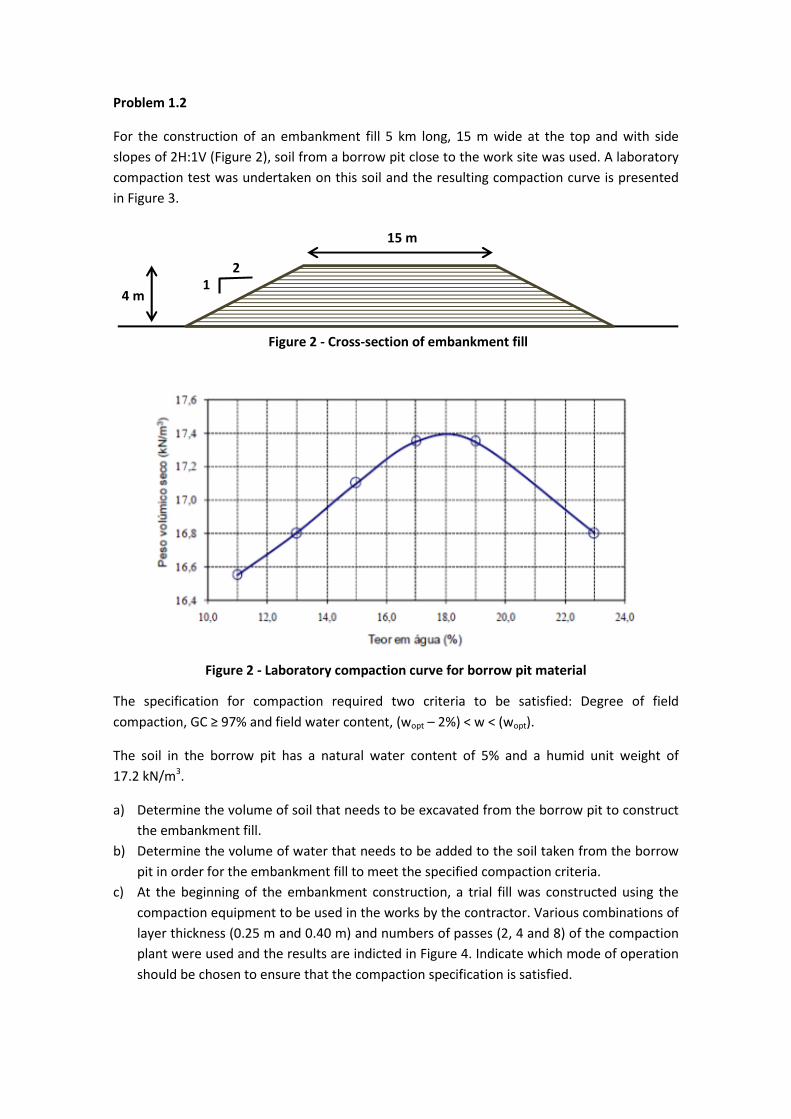
Problem 1.2

For the construction of an embankment fill 5 km long, 15 m wide at the top and with side

slopes of 2H:1V (Figure 2), soil from a borrow pit close to the work site was used. A laboratory

compaction test was undertaken on this soil and the resulting compaction curve is presented

in Figure 3.

Figure 2 - Laboratory compaction curve for borrow pit material

The specification for compaction required two criteria to be satisfied: Degree of field

compaction, GC ≥ 97% and field water content, (wopt – 2%) < w < (wopt).

The soil in the borrow pit has a natural water content of 5% and a humid unit weight of

17.2 kN/m3.

a) Determine the volume of soil that needs to be excavated from the borrow pit to construct

the embankment fill.

b) Determine the volume of water that needs to be added to the soil taken from the borrow

pit in order for the embankment fill to meet the specified compaction criteria.

c) At the beginning of the embankment construction, a trial fill was constructed using the

compaction equipment to be used in the works by the contractor. Various combinations of

layer thickness (0.25 m and 0.40 m) and numbers of passes (2, 4 and 8) of the compaction

plant were used and the results are indicted in Figure 4. Indicate which mode of operation

should be chosen to ensure that the compaction specification is satisfied.

15 m

4 m

2

1

Figure 2 - Cross-section of embankment fill

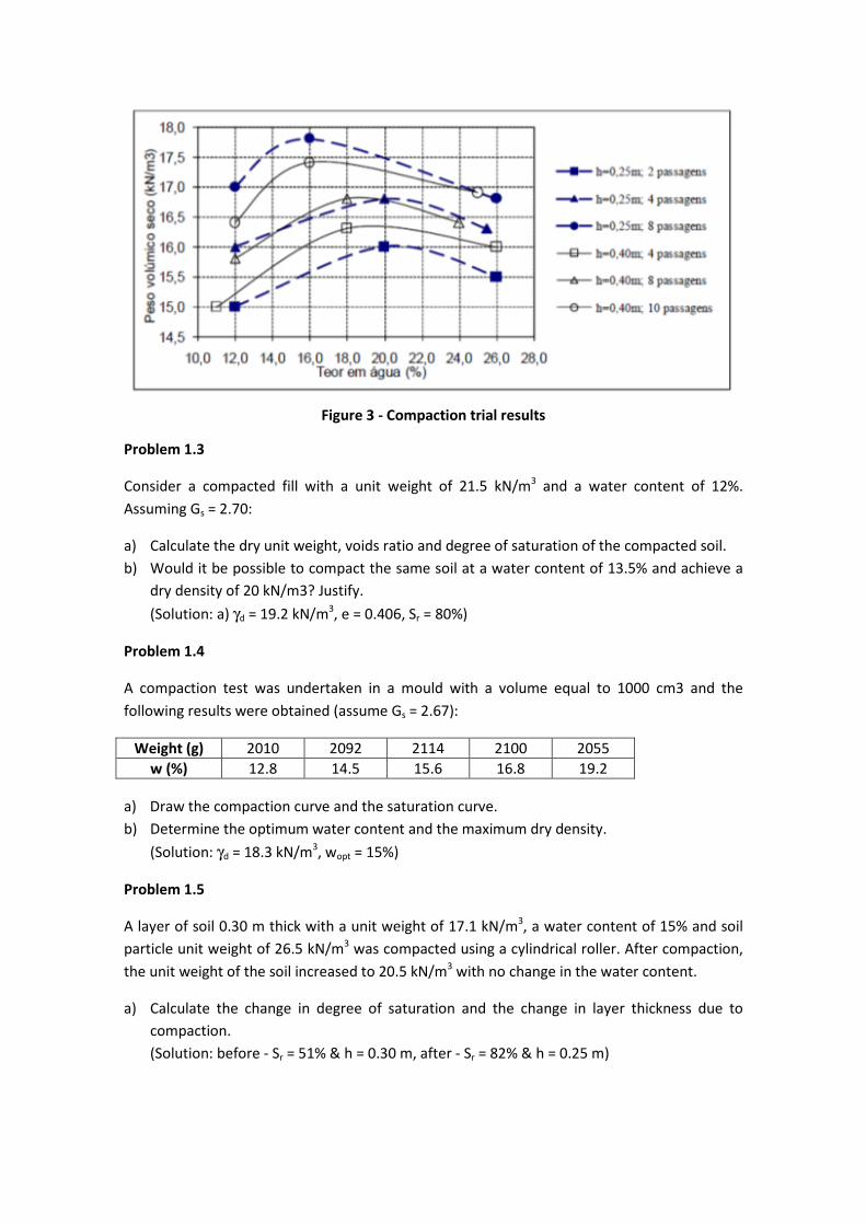
Figure 3 - Compaction trial results

Problem 1.3

Consider a compacted fill with a unit weight of 21.5 kN/m3 and a water content of 12%.

Assuming Gs = 2.70:

a) Calculate the dry unit weight, voids ratio and degree of saturation of the compacted soil.

b) Would it be possible to compact the same soil at a water content of 13.5% and achieve a

dry density of 20 kN/m3? Justify.

(Solution: a) γd = 19.2 kN/m3, e = 0.406, Sr = 80%)

Problem 1.4

A compaction test was undertaken in a mould with a volume equal to 1000 cm3 and the

following results were obtained (assume Gs = 2.67):

Weight (g) 2010 2092 2114 2100 2055

w (%) 12.8 14.5 15.6 16.8 19.2

a) Draw the compaction curve and the saturation curve.

b) Determine the optimum water content and the maximum dry density.

(Solution: γd = 18.3 kN/m3, wopt = 15%)

Problem 1.5

A layer of soil 0.30 m thick with a unit weight of 17.1 kN/m3, a water content of 15% and soil

particle unit weight of 26.5 kN/m3 was compacted using a cylindrical roller. After compaction,

the unit weight of the soil increased to 20.5 kN/m3 with no change in the water content.

a) Calculate the change in degree of saturation and the change in layer thickness due to

compaction.

(Solution: before - Sr = 51% & h = 0.30 m, after - Sr = 82% & h = 0.25 m)

Problem 1.6

To construct an embankment with a total volume of 175000 m3, 182000 m3 of fill was

obtained from a borrow pit. Laboratory compaction testing yielded values for γd,max =

16.2 kN/m3 and wopt = 12%. Assuming that the soil was compacted to the optimum state, the

natural water content of the borrow pit material is 6% and Gs = 2.63:

a) Determine the natural unit weight of the borrow pit material.

(Solution: γh = 16.5 kN/m3)

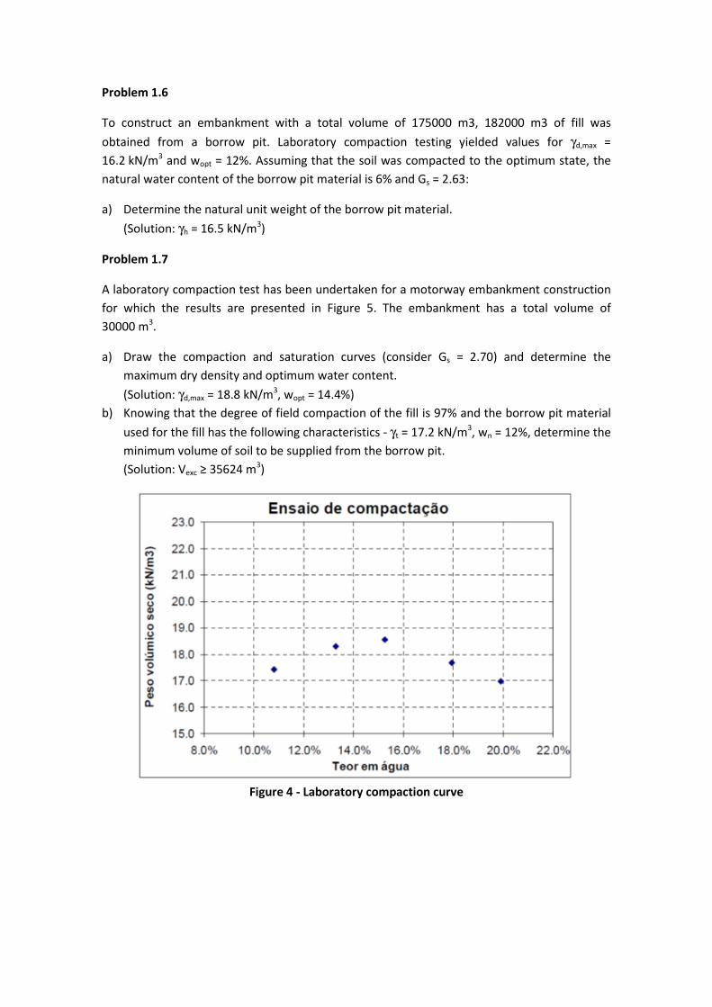
Problem 1.7

A laboratory compaction test has been undertaken for a motorway embankment construction

for which the results are presented in Figure 5. The embankment has a total volume of

30000 m3.

a) Draw the compaction and saturation curves (consider Gs = 2.70) and determine the

maximum dry density and optimum water content.

(Solution: γd,max = 18.8 kN/m3, wopt = 14.4%)

b) Knowing that the degree of field compaction of the fill is 97% and the borrow pit material

used for the fill has the following characteristics - γt = 17.2 kN/m3, wn = 12%, determine the

minimum volume of soil to be supplied from the borrow pit.

(Solution: Vexc ≥ 35624 m3)

Figure 4 - Laboratory compaction curve

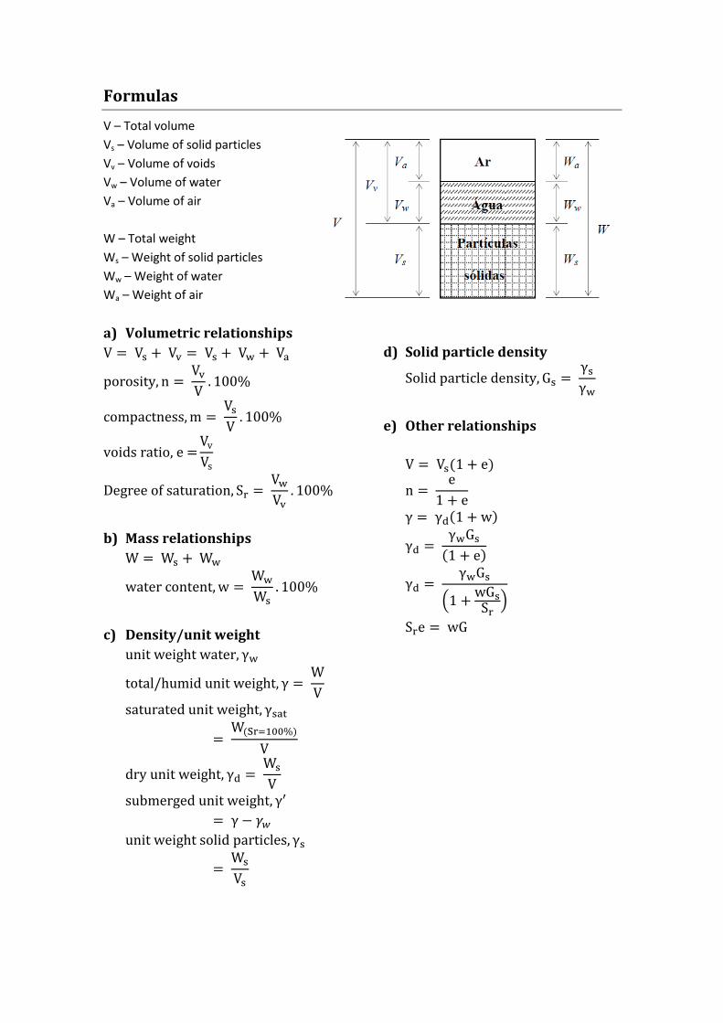
Formulas

V – Total volume

Vs – Volume of solid particles

Vv – Volume of voids

Vw – Volume of water

Va – Volume of air

W – Total weight

Ws – Weight of solid particles

Ww – Weight of water

Wa – Weight of air

a) Volumetric relationships V = V� +V� =V� +V� +VR

porosity, n = V�V . 100%

compactness,m = V�V . 100%

voidsratio,e=VvVs Degreeofsaturation, S¤ =V�V� . 100%

b) Mass relationships W =W� +W�

watercontent, w = W�W� . 100%

c) Density/unit weight unitweightwater, γ�

total/humidunitweight, γ = WV saturatedunitweight, γ�Rª=W.«¤mZ__%1V

dryunitweight, γ� =W�V submergedunitweight, γ­= γ − ®̄ unitweightsolidparticles, γ�=W�V�

d) Solid particle density Solidparticledensity, G� = γ�γ�

e) Other relationships

V = V�.1 + e1 n = e1 + e γ = γ�.1 + w1 γ� = γ�G�.1 + e1 γ� = γ�G�K1 + wG�S¤ L

S¤e = wG