Pilot Patterns and Power Loading in NC-OFDM

Cognitive Radios

Boyan Ventzislavov Soubachov

Thesis Presented for the Degree of

Doctor of Philosophy

in the Department of Electrical Engineering

University of Cape Town

October 2013

The copyright of this thesis vests in the author. No quotation from it or information derived from it is to be published without full acknowledgement of the source. The thesis is to be used for private study or non-commercial research purposes only.

Published by the University of Cape Town (UCT) in terms of the non-exclusive license granted to UCT by the author.

Unive

rsity

of C

ape

Town

ii

As the supervisor of the candidate, I approve this thesis for submission.

Name: Neco Ventura

Signed: ____________________________

Date: 1 October 2013________________

Signature removed

iii

Declaration

I hereby declare that the above thesis is my own unaided work, both in conception and

execution, and that apart from the normal guidance of my supervisor, I have received no

assistance apart from that as stated below. With the exceptions where stated, I have not

submitted the substance or any part of the thesis in the past, or is being submitted, or is to be

submitted for a degree at this University or at any other University.

I am now presenting this thesis for examination for the Degree of PhD in Electrical

Engineering, I also grant the University of Cape Town free license to reproduce the above

thesis in whole or in part for the purpose of research.

__________________________ 1 October 2013_____________

Boyan Ventzislavov Soubachov Date

iv

v

Abstract

Modern communications systems still use traditional spectrum licensing methods which

assign spectrum as an exclusive-use commodity to an entity. While this approach guarantees

no interference, it has been shown that most entities transmit information in bursts rather than

continuous streams which has consequently led to the inefficient use of radio spectrum.

Cognitive radios aim to correct this problem by utilising the spectrum of the licensed users

when the licensed users themselves are not using it. In theory, this is an optimal solution as it

would allow non-licensed users to exploit the inefficiencies of the licensed users while

maintaining a 'transparent' appearance to the users by changing their frequency band when

the cognitive radios detect that the licensed user has resumed the use of their own frequency

band.

The implementation of cognitive radios is widely proposed through the use of Orthogonal

Frequency Division Multiplexing (OFDM) modulation. In the special case of cognitive radios

however, the OFDM modulation scheme cannot simply be implemented without modification

due to the huge change in the basic laws of the transmission paradigm. The main reason

behind this is that the modulation scheme can no longer assume the contiguousness of its

band as well as the interference that may be caused by the cognitive radio users operating in

such close proximity to the licensed users. The research presented in this thesis namely

identified two areas of cognitive radio which addressed these issues. These were the power

loading and channel estimation areas.

The power loading aspect of cognitive radios dictates how power should be assigned

during modulation such that the interference caused by the cognitive radio to the licensed

users is kept below a fixed threshold. The power loading algorithm also aims to maximise the

throughput achieved by the cognitive radio given the fact that the licensed users nearby the

cognitive radio would be interfering with it. The channel estimation aspect on the other hand

aims to maximise the cognitive radio throughput through more accurate estimation of the

communications channel given the cognitive radio conditions employed. Both algorithms are

designed to solve the problem of introducing the aspect of non-contiguousness inherent in

cognitive radios to their traditional counterparts in OFDM where the modulation may be

considered contiguous (i.e. no cognitive radios).

vi

The work presented in this thesis describes the research conducted in these two areas and

analyses the currently existing, optimal solution for these two individual areas. More

importantly, however, is that it also identifies a contradiction between these two areas. The

contradiction is then addressed by providing a scientific and mathematical description of the

problem. An engineering solution is also provided with the derivation and development of the

optimal solution to this contradiction. The document shows an analysis of how the solution

would solve the imposed problem as well as exploring alternative venues of possible

solutions.

The document also shows an analysis of the proposed solution in terms of related

research. It was found that no other solution to this problem was posed. This is due to the fact

that in all the research done, this problem does not seem to have been identified by any other

research or related works. It is therefore believed that a novel approach and solution have

been proposed by the research work presented in this document to a critical implementation

problem which does not seem to have been discovered as of yet.

This thesis also presents the practical implementations possible of this optimal solution as

well as simulation results of these solutions. The optimal solution itself is well documented

and a general algorithm which may be used is demonstrated. The thesis however also

demonstrates sub-optimal solutions which may be used in place of the optimal solution for

practical situations where computing power or the amount of available device power is

limited. From simulation results, it was found that when using the optimal, proposed solution

the accuracy of the channel estimator could be increased (i.e. a decrease in error) by as much

as 10 dB relative to the current, static pilot patterns currently employed when using the

MMSE estimator. The results obtained when simulating the LS estimator were observed that

the overall estimator MSE did not significantly improve (reduce) when utilising the proposed

solution algorithm. The algorithm did however achieve its primary purpose of placing the

dynamic pilot symbols in the best position such that interference from the secondary users to

the primary users is kept below a specified threshold.

The document also proposes future avenues of research work which could be conducted

to further improve and build upon the proposed optimal and sub-optimal solutions as well as

any possible implementations and performance analysis.

vii

Acknowledgements

I wish to convey my gratefulness and sincere appreciation to a number of people who

have supported me and provided invaluable feedback during the duration of my postgraduate

studies.

I would firstly like to thank my parents Ventzislav Soubachov and Aneliia Soubachova as

well as my sister, Valya Soubachova for their unwavering encouragement and support, both

financially and morally. I would especially like to thank my parents for having the desire and

will needed to emigrate from my home country of Bulgaria with little more than strong

resolve just so that my sister and I would get a chance at building much better and fruitful

lives than would have otherwise been possible. Their resolve and determination has been a

great example for me to follow and without it, I doubt I would have gotten so far in my

pursuit for greater knowledge and achievement.

I would like to convey my gratitude to my supervisor, Neco Ventura who has been a great

guide and mentor throughout the duration of my studies. Without his initial advice of

pursuing the field of cognitive radio, I don't think I would have been able to get the chance of

learning so much about such an exciting technology. The advice I have received has been

invaluable in also allowing me to really delve deeper and deeper to seek a better

understanding of this field. I am completely certain that my time spent conducting research

will be of even more value to myself and others in the future. I also wish the best of luck to

Neco in his future running of the Centre of Excellence for Broadband Networks as I am sure

that ever greater research and alumni will be produced by the centre.

I would also like to give thanks to the current and past members of the Communications

Research Group at the University of Cape Town. The input and discussions I have received

from my fellow members has been invaluable in shaping and refining my research. The

critique and discussions I have had with Eugene Golovins have been very informative and

have especially shaped my research. I hope that in the ironic twist of fate, he has a very

successful academic career under the mentorship of my undergraduate thesis supervisor at my

previous alma mater.

I would like to express a special expression of gratitude goes out to the many people I

have met in conferences over the years. It has been most joyous meeting and connecting with

people from different cultures and different backgrounds all sharing the same deep desire to

viii

have their work be a positive improvement for humanity, even if it is that slightest little bit.

The invaluable feedback I have also received has been nothing short of astounding and has

shaped the direction, both in terms of technical as well as practical, of my research

continually. This has been instrumental in allowing me to continually challenge and improve

myself.

Finally, I would like to thank all my close friends in all my different home towns for the

constant support and encouragement provided. It has been a difficult journey with many ups

and downs but I am grateful for having support during both the good times and the bad.

ix

Foreword

The research work which has been concluded and summarised in this thesis originally

commenced in January 2010. The work originally started as a Masters degree project (MSc)

under the supervision of Neco Ventura. Since its commencement, the work involved

intensive literature study which eventually led to the discovery of a contradiction in the areas

of pilot patterns and power loading in NC-OFDM cognitive radios.

During May 2011, an application was made to the Doctoral Degrees Board of the

University of Cape Town to upgrade the Masters degree to a Doctoral (PhD) as per the

recommendation of Neco deeming that the research work conducted would satisfactorily

meet the requirements for a doctoral degree. The upgrade was approved that same month.

For the whole duration of the research project, it was conducted at the University of Cape

Town in the Centre for Broadband Networks and Applications. Side-projects were also

undertaken during the duration of the research such as the familiarisation with the OpenEPC

system by invitation of the Fraunhofer Institute at TU Berlin as well as the design and

mentoring of final-year projects to be performed by undergraduate students at the University.

The research conducted then allowed for scientific progress, specifically in identifying,

modelling and solving the contradiction which would exist should an NC-OFDM cognitive

radio be implemented using both the optimal pilot pattern algorithms and optimal power

loading algorithms currently proposed for implementation.

The research resulted in several publications during its progression. These are elaborated

in later sections.

x

xi

Table of Contents

1. Introduction ................................................................................................................. 1

1.1. Cognitive Radios as a Solution to Spectrum Crowding .......................................... 2

1.2. Non-Contiguous OFDM .......................................................................................... 4

1.3. Interference Concerns and Power Loading ............................................................. 6

1.4. Channel Estimation and Equalisation .................................................................... 10

1.5. Research Statement and Goals .............................................................................. 16

1.5.1. Research questions ......................................................................................... 16

1.5.2. Requirements of proposed solution ................................................................ 17

1.5.3. Comparison to current solutions .................................................................... 18

1.5.4. Thesis Contributions ...................................................................................... 19

1.5.5. Research Methodology ................................................................................... 19

1.6. List of Publications ................................................................................................ 20

1.7. Thesis Structure ..................................................................................................... 21

2. Background ............................................................................................................... 23

2.1. Single/Multi-Carrier Modulation and the Shannon Limit ..................................... 23

2.2. Current Spectrum Licensing and Spectrum as a Commodity ................................ 29

3. System Models .......................................................................................................... 37

3.1. OFDM-based System Models ............................................................................... 37

3.1.1. OFDM modulation theory .............................................................................. 38

3.2. Channel and Interference Models .......................................................................... 43

3.2.1. Power density spectrum of signals ................................................................. 44

3.2.2. PU-to-SU interference .................................................................................... 45

3.2.3. SU-to-PU interference .................................................................................... 46

3.3. Optimal Power Loading Algorithm ....................................................................... 47

3.4. LS Estimator Error................................................................................................. 48

xii

3.4.1. Pilot symbol error ........................................................................................... 48

3.4.2. Interpolation error .......................................................................................... 49

3.5. MMSE Estimator Error ......................................................................................... 51

3.6. Optimal Pilot Pattern Algorithm............................................................................ 54

3.7. Contributions ......................................................................................................... 56

4. Optimal Pilot Patterns Using Optimal Power Loading ............................................. 57

4.1. Formulation as a Constrained Multivariate Optimisation Problem ....................... 57

4.2. Generalised Solution and Algorithm ..................................................................... 62

4.2.1. 1-dimensional implementation ....................................................................... 63

4.2.2. 2-dimensional implementation ....................................................................... 64

4.3. LS Estimator Heuristic .......................................................................................... 66

4.4. MMSE Estimator Heuristic ................................................................................... 69

4.5. Algorithm Complexity and Sub-Optimal Solutions .............................................. 71

4.5.1. Algorithm complexity .................................................................................... 72

4.5.2. Windowing and sub-optimal algorithm.......................................................... 73

4.5.3. Sub-optimal heuristics .................................................................................... 76

4.5.4. Heuristic function approximations ................................................................. 77

4.5.5. Computational Complexity Implications ....................................................... 78

4.6. Comparison to Similar Solutions ........................................................................... 79

5. Simulation Details and Results ................................................................................. 80

5.1. Simulation Parameters ........................................................................................... 80

5.1.1. 1-dimensional simulation parameters............................................................. 83

5.1.2. 2-dimensional simulation parameters............................................................. 84

5.2. Simulation Results ................................................................................................. 85

5.2.1. 1-dimensional, optimal solutions ................................................................... 86

5.2.1.1. Least-squares estimator .............................................................................. 86

5.2.1.2. MMSE estimator......................................................................................... 91

xiii

5.2.2. 2-dimensional, optimal solutions ................................................................... 97

5.2.2.1. LS channel estimator .................................................................................. 98

5.2.2.2. MMSE channel estimator ......................................................................... 103

5.2.3. Sub-optimal solutions ................................................................................... 114

5.2.3.1. LS estimator results .................................................................................. 114

5.2.3.2. MMSE estimator results ........................................................................... 119

5.3. Comparison to Related Work .............................................................................. 125

6. Conclusions and Future Work ................................................................................. 127

6.1. Conclusions ......................................................................................................... 131

6.2. Future Work ......................................................................................................... 140

6.2.1. Series expansion for analytic solution .......................................................... 141

6.2.2. Pulse-shaping functions................................................................................ 142

6.2.3. Extension to MIMO systems ........................................................................ 142

6.2.4. Algorithm optimisations ............................................................................... 144

References ........................................................................................................................ 146

Appendices ...................................................................................................................... 150

Appendix A: KKT constraints of the optimisation problem ....................................... 152

Appendix B: Derivation of MMSE estimator ............................................................. 159

Appendix C: Analysis of polynomial interpolant error bound ................................... 164

Appendix D: Different terrain types when modelling channels ................................. 173

Appendix E: Mathematical description of Rician and Rayleigh fading ..................... 175

xiv

List of Figures

Figure 1: Visualisation of overlay cognitive radio access scheme 3

Figure 2: Visualisation of underlay cognitive radio access scheme 4

Figure 3: Demonstration of interference mitigation in NC-OFDM 5

Figure 4: Traditional, water-filling power loading method for contiguous

OFDM 7

Figure 5: Spectral roll-off and its effects due to non-ideality 8

Figure 6: Rough demonstration of the optimal power loading algorithm 9

Figure 7: Demonstration of block type pilot pattern 12

Figure 8: Demonstration of comb type pilot pattern 12

Figure 9: Diagonal and scattered types of pilot patterns 14

Figure 10: The proposed optimal pilot pattern algorithm for NC-OFDM

cognitive radios 15

Figure 11: Naming conventions in the OFDM time-frequency grid 29

Figure 12: Urban spectrum occupancy for 0 - 3 GHz 31

Figure 13: Urban spectrum occupancy by different uses for 2008 32

Figure 14: Urban spectrum occupancy by different uses for 2009 33

Figure 15: Urban spectrum occupancy by different uses for 2010 34

Figure 16: Spectrum occupancy on a weekly basis for 2009, urban area 35

Figure 17: Sampling points and orthogonal sub-carriers of OFDM 40

Figure 18: Cyclic prefix and its use in OFDM 42

Figure 19: The OFDM signal processing chain 43

Figure 20: The proposed NC-OFDM optimal pilot placement algorithm

xv

for both narrow- and wideband 55

Figure 21: Visualisation of the normalised SU-to-PU interference 61

Figure 22: Visual depiction of the windowing performed to achieve a

sub-optimal implementation of the solution algorithm 75

Figure 23: Error heuristic value for 1-D, LS for different PU

transmit powers 87

Figure 24: Error heuristic value for 1-D, LS for different PU transmit

bandwidths 89

Figure 25: Error heuristic value for 1-D, LS for different PU interference

thresholds 90

Figure 26: Narrowband view of error heuristic value for 1-D, MMSE for

different PU transmit power 91

Figure 27: Wideband view of error heuristic value for 1-D, MMSE for

different PU transmit power 92

Figure 28: Error heuristic value for 1-D, MMSE for different PU transmit

bandwidths 94

Figure 29: Error heuristic value for 1-D, MMSE for different PU

interference thresholds 94

Figure 30: Exaggerated case, error heuristic value for 1-D, MMSE for

different PU transmit bandwidths 96

Figure 31: Error function value for 2-D, LS for a static system 99

Figure 32: Error function value for 2-D, LS for a dynamic system 100

Figure 33: Error function value for 2-D, LS for a dynamic system where

xvi

the PU bandwidth is uniformly varying 101

Figure 34: Optimal time-frequency grid for 2-D, LS scenario with a

dynamic system 102

Figure 35: Error function value for 2-D, MMSE for a static system 103

Figure 36: Error function value for 2-D, MMSE for a dynamic system 104

Figure 37: Optimal time-frequency grid for 2-D, MMSE scenario with a

static system 105

Figure 38: Error function value for 2-D, MMSE for a dynamic system

where the PU bandwidth is uniformly varying 106

Figure 39: Optimal time-frequency grid for 2-D, MMSE scenario with a

dynamic system 108

Figure 40: NMSE per OFDM symbol for the MMSE estimator 109

Figure 41: MSE per OFDM symbol for the MMSE estimator 110

Figure 42: Comparison for NMSE between optimal solution algorithm and

static pilot pattern for the MMSE estimator 111

Figure 43: MSE per OFDM symbol for the optimal and sub-optimal

solution algorithm for the LS estimator 115

Figure 44: Computational time for optimal and sub-optimal algorithms using

the LS estimator 117

Figure 45: Cumulative computational time for optimal and sub-optimal, LS

solution algorithm 118

Figure 46: MSE comparison per OFDM symbol for the MMSE estimator

between optimal and sub-optimal solution algorithm

xvii

implementations 120

Figure 47: Computational time for optimal and sub-optimal algorithms

using the MMSE estimator 121

Figure 48: Cumulative computational time for optimal and sub-optimal,

MMSE solution algorithm 122

Figure B.1: Robust channel auto-correlation matrix 162

Figure C.1: Matrix inversion time analysis 166

Figure C.2: Polynomial interpolator trade-off 168

Figure C.3: Demonstration of the Runge phenomenon 170

Figure C.4: Chebyshev node spacing for interpolation error minimisation 171

Figure E.1: Rayleigh and Rician PDFs 177

Figure E.2: Rayleigh and Rician CDFs 178

xviii

List of Tables

Table 1: Classification of channel models by terrain type 82

Table 2: Simulation parameters for 1-dimensional estimator scenarios 84

Table 3: Additional simulation parameters for 2-dimensional estimator scenarios 85

Table D.4: Channel model parameters by different terrain types 174

xix

Acronyms

AM Amplitude Modulation

AWGN Additive White Gaussian Noise

BTS Base Transceiver Station

CDF Cumulative Distribution Function

CFR Channel Frequency Response

CIR Channel Impulse Response

CNR Carrier-to-Noise Ratio

CP Cyclic Prefix

CR Cognitive Radio

DFT Discrete Fourier Transform

DMT Discrete Multitone

DSA Dynamic Spectrum Access

DSL Digital Subscriber Line

EIRP Effective Isotropically Radiated Power

FFT Fast Fourier Transform

FHSS Frequency-Hopping Spread Spectrum

FIR Finite Impulse Response

FM Frequency Modulation

ICI Inter-Channel Interference

IEEE Institute for Electrical and Electronics Engineers

i.i.d. Independent and Identically Distributed

ISI Inter-Symbol Interference

xx

ISM Industrial, Scientific and Medical

KKT Karush-Kuhn-Tucker

LOS Line of Sight

LS Least Squares

LTE Long Term Evolution

MC Multi-carrier

MIMO Multiple Input, Multiple Output

ML Maximum Likelihood

MLSE Maximum Likelihood Sequence Estimator

MMSE Minimum Mean Squared Error

MSE Mean Squared Error

NC-OFDM Non-Contiguous Orthogonal Frequency Division Multiplexing

NLOS Non-Line of Sight

NMSE Normalised Mean Square Error

OFDM Orthogonal Frequency Division Multiplexing

OFDMA Orthogonal Frequency Division Multiple Access

OOB Out-of-Band

PAPR Peak-to-Average Power Ratio

PDF Probability Density Function

PDP Power-Delay Profile

PDPR Pilot-to-Data Power Ratio

PDS Power Density Spectrum

POTS Plain Old Telephone Service

xxi

PSAM Pilot Symbol Assisted Modulation

PSD Power Spectral Density

PU Primary User

SC-FDMA Single Carrier Frequency Division Multiple Access

SNR Signal-to-Noise Ratio

SSB Single-Sideband

SU Secondary User

SUI Stanford University Interim

SVD Singular Value Decomposition

UWB Ultra-Wideband

VSB Vestigial Sideband

WLAN Wireless Local Area Network

WSSUS Wide-Sense Stationary Uncorrelated Scattering

ZF Zero-Forcing

xxii

Notations

[ ] Vector consisting of elements where [ ]

[ ] Matrix consisting of elements , [ ] (row),

[ ] (column)

Moore-Penrose pseudo-inverse of

Transpose of

Herimitian transpose of

Complex conjugate of

Del operator (vector partial derivative)

Fourier transform of

Fourier matrix

iff If and only if

Identity matrix of size

⌈ ⌉ Ceiling, i.e. round up to nearest integer

⌊ ⌋ Floor, i.e. round down to nearest integer

[ ] Value of discrete function at index n

Value of continuous function at time t

Imaginary unit

Dirac delta function

Is an element of

Is not an element of

Circular convolution

xxiii

Convolution

Si Sine integral

xxiv

This page intentionally left blank

1

1. Introduction

Modern communications systems are characterised by an ever growing need for higher

transmission rates. Through the use of many innovative techniques such as multi-carrier

modulation, we have reached a point where most modern communications systems are

described as capacity-approaching as they are very close to a theoretical limit (known as the

Shannon Limit) on the maximum possible information rate over a noisy medium. This means

that in order to be able to support the ever-growing demand for higher information transfer

rates, there has been great pressure to utilise the practically available spectrum more

efficiently. This has led to the development of a family of technologies known as cognitive

radio (CR).

Cognitive radios attempt to address the inefficiencies associated with the current

licensing models where an entity obtains an exclusive right to use a fixed bandwidth of the

spectrum. This means that when the licensed entity is not using its band, it remains empty and

unused as no other entity is by law allowed to use the band. Cognitive radio aims to address

this problem by developing devices which are able to utilise the licensed bands when the

licensees themselves are not using them. This is one aspect as defined in the description of a

cognitive radio which is defined by Mitola by stating that cognitive radios are devices which

are "sufficiently computationally intelligent about radio resources and related computer-to-

computer communications to detect user communications needs as a function of use context

and to provide radio resources and wireless services most appropriate to those needs" [1].

From the description, the cognitive radio would adjust its modulation parameters to meet the

needs of its users. The main aspect of the cognitive radio which would provide a promising

solution to the problem of spectrum crowding is the channel access paradigm known as

Dynamic Spectrum Access (DSA).

Dynamic spectrum access is a design principle whereby the radio device is designed

around the premise of adaptability and agility in terms of the centre frequency of operation

used for modulation. This means that instead of utilising a fixed frequency band for

operation, the radio is able to adapt and change its centre frequency of operation to a more

suitable band of operation or a random one (for the purposes of security) to achieve a more

efficient utilisation of spectrum. As such, if the goal of a cognitive radio is defined to be

spectral usage efficiency, it could be used to alleviate and even solve the problem of spectrum

2

shortage. The DSA aspect of a cognitive radio device could then be used to access licensed

spectrum when the licensee of the band of interest is not using the spectrum themselves.

As CR devices would imply a whole paradigm shift from traditional fixed spectrum

access to dynamic spectrum access, there are a big number of challenges associated with

them. Two of these problems concern the aspects of controlling the interference between

legacy, licensed users and cognitive, unlicensed users as well as co-ordination such that the

maximum data rate can be obtained from the unused spectrum that is available. The research

presented in this document addresses a problem identified with both of these aspects and a

detailed explanation is presented in subsequent sections.

The research methodology is then explained with the focus on describing the research

statement, the research goals and a comparison to existing solutions. These were used to

provide a systematic framework for the expectation of deliverables as well as to identify

which challenges had the highest need to be addressed and consequently to aid in the efficient

allocation of research time and effort.

1.1. Cognitive Radios as a Solution to Spectrum Crowding

The problems inherent in spectrum crowding, licensing and under-utilisation have created

a unique problem where a paradigm shift is needed to ensure that the information transfer rate

demands of future applications are met. Cognitive radios are in fact a paradigm shift from the

old ways of communication where the intelligence is centralised (i.e., at the network

management level) to a new paradigm where intelligence moves to the edges of the network

(the end-user devices) [1]. This means that the consumer devices are enabled to perform

cognition as well as take action in changing their parameters dynamically as the user's

requirements change whilst doing it transparently of the user.

As the main aspect of focus in this research is the DSA component of a CR system, there

are two types of DSA for CRs, namely underlay access and overlay access. These two aspects

are both unique in their approach but both of their goals involve for the cognitive radio users,

also known as the Secondary Users (SUs), to be able to access the spectrum of the licensed

users, also known as Primary Users (PUs) without causing any interference noticeable to the

PUs.

3

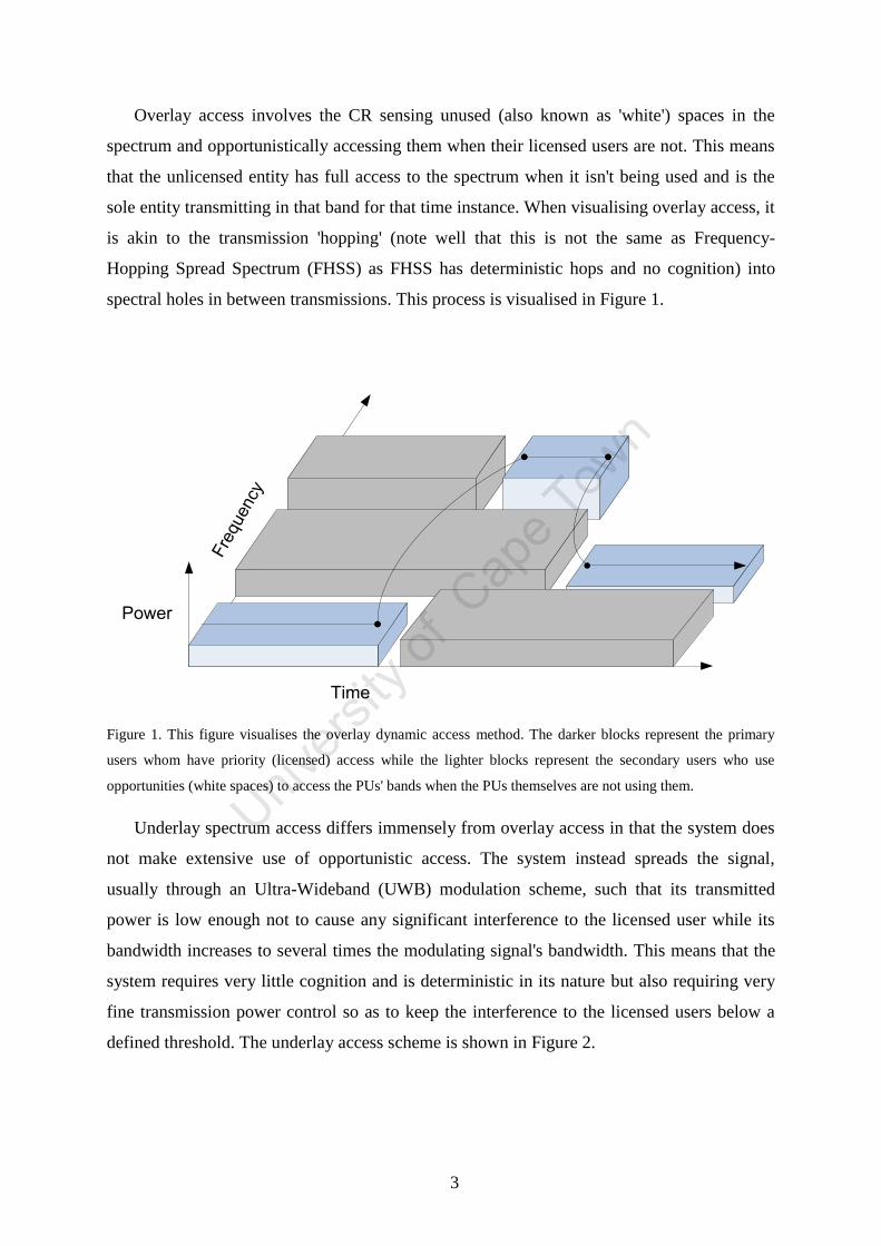
Overlay access involves the CR sensing unused (also known as 'white') spaces in the

spectrum and opportunistically accessing them when their licensed users are not. This means

that the unlicensed entity has full access to the spectrum when it isn't being used and is the

sole entity transmitting in that band for that time instance. When visualising overlay access, it

is akin to the transmission 'hopping' (note well that this is not the same as Frequency-

Hopping Spread Spectrum (FHSS) as FHSS has deterministic hops and no cognition) into

spectral holes in between transmissions. This process is visualised in Figure 1.

Power

Time

Fre

quency

Figure 1. This figure visualises the overlay dynamic access method. The darker blocks represent the primary

users whom have priority (licensed) access while the lighter blocks represent the secondary users who use

opportunities (white spaces) to access the PUs' bands when the PUs themselves are not using them.

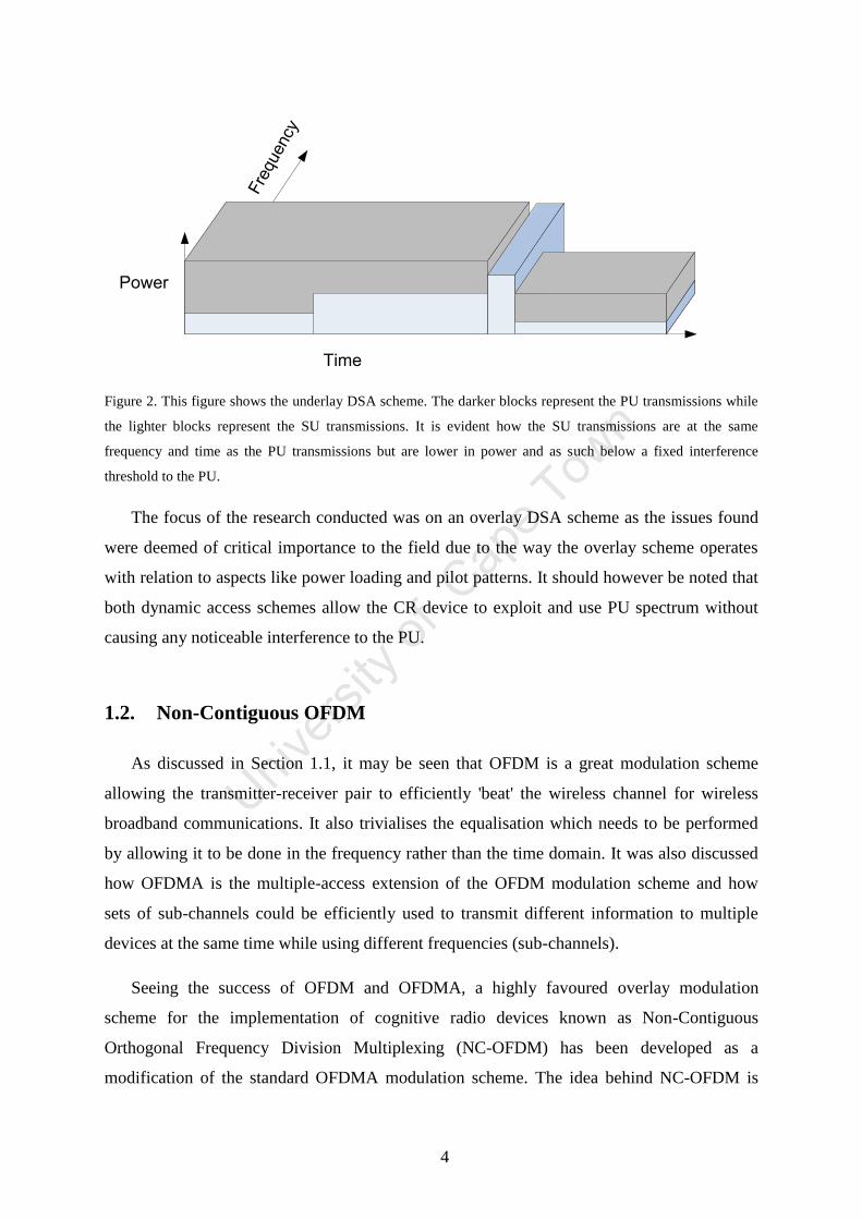
Underlay spectrum access differs immensely from overlay access in that the system does

not make extensive use of opportunistic access. The system instead spreads the signal,

usually through an Ultra-Wideband (UWB) modulation scheme, such that its transmitted

power is low enough not to cause any significant interference to the licensed user while its

bandwidth increases to several times the modulating signal's bandwidth. This means that the

system requires very little cognition and is deterministic in its nature but also requiring very

fine transmission power control so as to keep the interference to the licensed users below a

defined threshold. The underlay access scheme is shown in Figure 2.

4

Power

Time

Fre

quency

Figure 2. This figure shows the underlay DSA scheme. The darker blocks represent the PU transmissions while

the lighter blocks represent the SU transmissions. It is evident how the SU transmissions are at the same

frequency and time as the PU transmissions but are lower in power and as such below a fixed interference

threshold to the PU.

The focus of the research conducted was on an overlay DSA scheme as the issues found

were deemed of critical importance to the field due to the way the overlay scheme operates

with relation to aspects like power loading and pilot patterns. It should however be noted that

both dynamic access schemes allow the CR device to exploit and use PU spectrum without

causing any noticeable interference to the PU.

1.2. Non-Contiguous OFDM

As discussed in Section 1.1, it may be seen that OFDM is a great modulation scheme

allowing the transmitter-receiver pair to efficiently 'beat' the wireless channel for wireless

broadband communications. It also trivialises the equalisation which needs to be performed

by allowing it to be done in the frequency rather than the time domain. It was also discussed

how OFDMA is the multiple-access extension of the OFDM modulation scheme and how

sets of sub-channels could be efficiently used to transmit different information to multiple

devices at the same time while using different frequencies (sub-channels).

Seeing the success of OFDM and OFDMA, a highly favoured overlay modulation

scheme for the implementation of cognitive radio devices known as Non-Contiguous

Orthogonal Frequency Division Multiplexing (NC-OFDM) has been developed as a

modification of the standard OFDMA modulation scheme. The idea behind NC-OFDM is

5

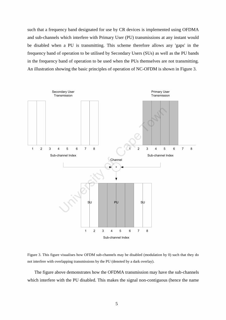
such that a frequency band designated for use by CR devices is implemented using OFDMA

and sub-channels which interfere with Primary User (PU) transmissions at any instant would

be disabled when a PU is transmitting. This scheme therefore allows any 'gaps' in the

frequency band of operation to be utilised by Secondary Users (SUs) as well as the PU bands

in the frequency band of operation to be used when the PUs themselves are not transmitting.

An illustration showing the basic principles of operation of NC-OFDM is shown in Figure 3.

1 2 3 4 5 6 7 8 1 2 3 4 5 6 7 8

Sub-channel Index Sub-channel Index

1 2 3 4 5 6 7 8

Sub-channel Index

+

Secondary User

Transmission

Primary User

Transmission

SU PU SU

Channel

Figure 3. This figure visualises how OFDM sub-channels may be disabled (modulation by 0) such that they do

not interfere with overlapping transmissions by the PU (denoted by a dark overlay).

The figure above demonstrates how the OFDMA transmission may have the sub-channels

which interfere with the PU disabled. This makes the signal non-contiguous (hence the name

6

NC-OFDMA) in the frequency domain, allowing for optimal utilization and exploitation of

any unused spectrum in both the time and frequency domains.

1.3. Interference Concerns and Power Loading

In the overlay DSA scheme as described in Section 1.1, it is expected that for optimal

spectral utilisation the SU transmission will be adjacent to the PU transmissions in the

frequency domain. As all systems are non-ideal, this means that some energy from the SU

will roll-off into the PU as well as energy from the PU to the SU. This in turn means that

there will be an increase in PU-to-SU as well as SU-to-PU interference. Since the principles

of cognitive radio require that the SU keep the interference to the PU below a fixed, design

specified threshold this means that power should be assigned intelligently to different sub-

channels of the SU signal such that the interference to the PU is kept below the specified

threshold in order to ensure that the interference effects imposed on the PU are negligible.

The aspect of assigning the transmission power per sub-channel according to a defined

algorithm is known as power loading. There are many power loading algorithms which have

been proposed but there exist optimal algorithms for both OFDM and NC-OFDM modulation

schemes.

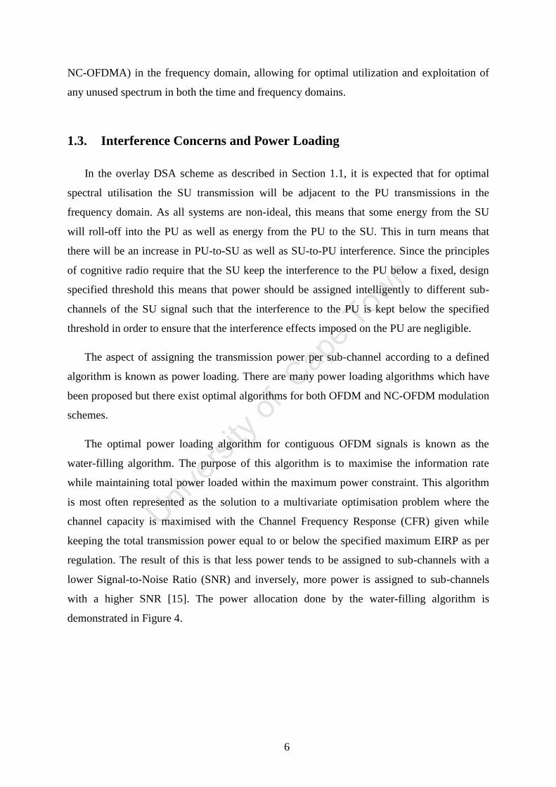
The optimal power loading algorithm for contiguous OFDM signals is known as the

water-filling algorithm. The purpose of this algorithm is to maximise the information rate

while maintaining total power loaded within the maximum power constraint. This algorithm

is most often represented as the solution to a multivariate optimisation problem where the

channel capacity is maximised with the Channel Frequency Response (CFR) given while

keeping the total transmission power equal to or below the specified maximum EIRP as per

regulation. The result of this is that less power tends to be assigned to sub-channels with a

lower Signal-to-Noise Ratio (SNR) and inversely, more power is assigned to sub-channels

with a higher SNR [15]. The power allocation done by the water-filling algorithm is

demonstrated in Figure 4.

7

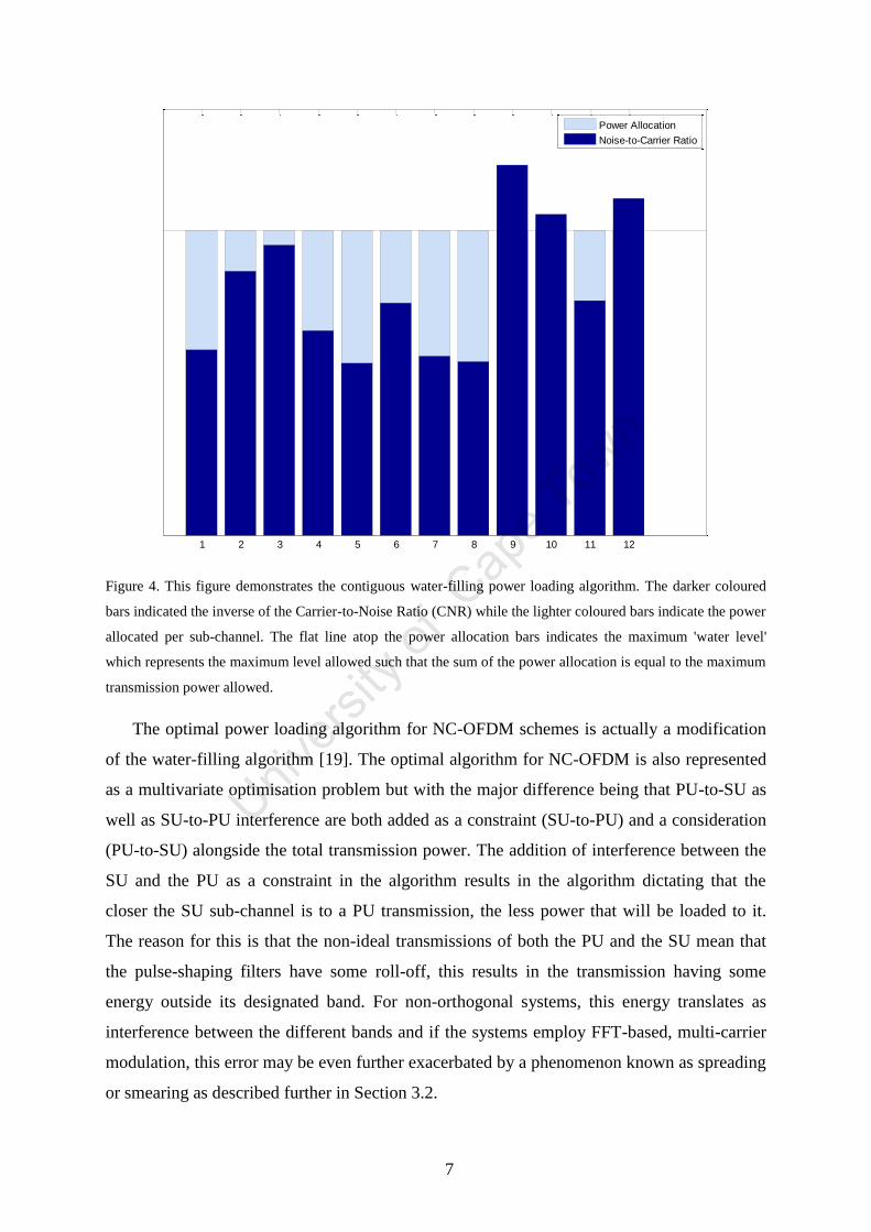
Figure 4. This figure demonstrates the contiguous water-filling power loading algorithm. The darker coloured

bars indicated the inverse of the Carrier-to-Noise Ratio (CNR) while the lighter coloured bars indicate the power

allocated per sub-channel. The flat line atop the power allocation bars indicates the maximum 'water level'

which represents the maximum level allowed such that the sum of the power allocation is equal to the maximum

transmission power allowed.

The optimal power loading algorithm for NC-OFDM schemes is actually a modification

of the water-filling algorithm [19]. The optimal algorithm for NC-OFDM is also represented

as a multivariate optimisation problem but with the major difference being that PU-to-SU as

well as SU-to-PU interference are both added as a constraint (SU-to-PU) and a consideration

(PU-to-SU) alongside the total transmission power. The addition of interference between the

SU and the PU as a constraint in the algorithm results in the algorithm dictating that the

closer the SU sub-channel is to a PU transmission, the less power that will be loaded to it.

The reason for this is that the non-ideal transmissions of both the PU and the SU mean that

the pulse-shaping filters have some roll-off, this results in the transmission having some

energy outside its designated band. For non-orthogonal systems, this energy translates as

interference between the different bands and if the systems employ FFT-based, multi-carrier

modulation, this error may be even further exacerbated by a phenomenon known as spreading

or smearing as described further in Section 3.2.

1 2 3 4 5 6 7 8 9 10 11 12

Power Allocation

Noise-to-Carrier Ratio

8

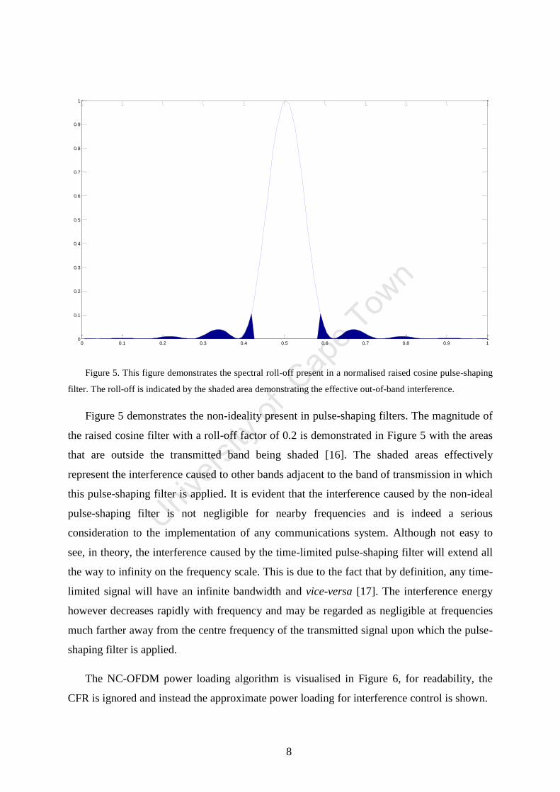
Figure 5. This figure demonstrates the spectral roll-off present in a normalised raised cosine pulse-shaping

filter. The roll-off is indicated by the shaded area demonstrating the effective out-of-band interference.

Figure 5 demonstrates the non-ideality present in pulse-shaping filters. The magnitude of

the raised cosine filter with a roll-off factor of 0.2 is demonstrated in Figure 5 with the areas

that are outside the transmitted band being shaded [16]. The shaded areas effectively

represent the interference caused to other bands adjacent to the band of transmission in which

this pulse-shaping filter is applied. It is evident that the interference caused by the non-ideal

pulse-shaping filter is not negligible for nearby frequencies and is indeed a serious

consideration to the implementation of any communications system. Although not easy to

see, in theory, the interference caused by the time-limited pulse-shaping filter will extend all

the way to infinity on the frequency scale. This is due to the fact that by definition, any time-

limited signal will have an infinite bandwidth and vice-versa [17]. The interference energy

however decreases rapidly with frequency and may be regarded as negligible at frequencies

much farther away from the centre frequency of the transmitted signal upon which the pulse-

shaping filter is applied.

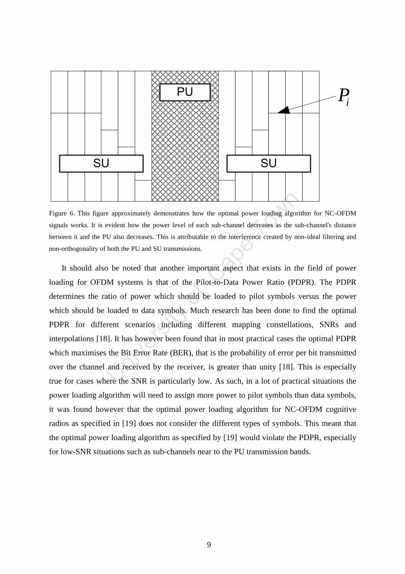
The NC-OFDM power loading algorithm is visualised in Figure 6, for readability, the

CFR is ignored and instead the approximate power loading for interference control is shown.

0 0.1 0.2 0.3 0.4 0.5 0.6 0.7 0.8 0.9 10

0.1

0.2

0.3

0.4

0.5

0.6

0.7

0.8

0.9

1

9

PU

SUSU

iP

Figure 6. This figure approximately demonstrates how the optimal power loading algorithm for NC-OFDM

signals works. It is evident how the power level of each sub-channel decreases as the sub-channel's distance

between it and the PU also decreases. This is attributable to the interference created by non-ideal filtering and

non-orthogonality of both the PU and SU transmissions.

It should also be noted that another important aspect that exists in the field of power

loading for OFDM systems is that of the Pilot-to-Data Power Ratio (PDPR). The PDPR

determines the ratio of power which should be loaded to pilot symbols versus the power

which should be loaded to data symbols. Much research has been done to find the optimal

PDPR for different scenarios including different mapping constellations, SNRs and

interpolations [18]. It has however been found that in most practical cases the optimal PDPR

which maximises the Bit Error Rate (BER), that is the probability of error per bit transmitted

over the channel and received by the receiver, is greater than unity [18]. This is especially

true for cases where the SNR is particularly low. As such, in a lot of practical situations the

power loading algorithm will need to assign more power to pilot symbols than data symbols,

it was found however that the optimal power loading algorithm for NC-OFDM cognitive

radios as specified in [19] does not consider the different types of symbols. This meant that

the optimal power loading algorithm as specified by [19] would violate the PDPR, especially

for low-SNR situations such as sub-channels near to the PU transmission bands.

10

1.4. Channel Estimation and Equalisation

As information is transmitted at a bandwidth higher than the channel coherence

bandwidth, ISI will occur. This means that the channel frequency response for the band of

interest will be non-flat and will differ over the band of interest. In order to obtain the correct

transmitted symbol in each sub-channel before any fading effects imposed by the channel, it

is necessary to negate the non-flat fading effects through a process called equalisation.

As ISI introduced by the channel is a multiplicative effect, the simplest way it may be

negated is by multiplying the OFDM symbol by the inverse of the CFR. This process is

known as Zero-Forcing (ZF) due to the fact that it brings the ISI down to zero in a noise-free

environment as the multiplicative effect of the non-flat fading would be ideally cancelled by a

division done during the equalisation process.

The ZF equalisation method is ideal and optimal in a noiseless environment [4]. In terms

of regression analysis the channel frequency response, which is inverted to perform the ZF

equalisation, needs to be estimated. This estimate is known as the Least Squares (LS)

estimate.

There are two methods of channel estimation, namely blind estimation and Pilot Symbol

Assisted Modulation (PSAM). Blind channel estimation attempts to estimate the channel's

frequency response without any a priori information. This means that no information is

transmitted for the purpose of channel estimation and as such all transmitted information is

data and the full time-frequency grid of the OFDM transmission is used for data symbols. On

the other hand, PSAM involves the transmission of some a priori information placed in a

specific pattern on the time-frequency grid of the OFDM frame. Known pilot symbols would

be inserted into positions and as such a pilot pattern would form which is known by the

receiver a priori. This means that the receiver can gauge the exact effect plus noise the

channel had on the symbol and therefore form a channel estimate.

An alternative way in estimating the channel frequency response and performing

equalisation is known as the Minimum Mean Squared Error (MMSE) estimate. When

performing LS estimation, the channel frequency response is attempted to be obtained by

dividing the received pilot symbol by the transmitted pilot symbol, as such this would

provide us with the multiplicative component caused by ISI as well as a noise component

added by AWGN. As the ZF equalisation involves multiplying the received OFDM symbol

11

by the inverse of the estimated channel response, it could result in greatly increasing the

additive noise component of the estimate for points where the CFR is very small due to the

very large inverse. The MMSE estimator attempts to mitigate this issue by not attempting to

completely eliminate ISI through division but rather to minimise the total power of both the

multiplicative ISI and additive noise components imposed on the transmission by the channel

due to the effects of ISI and AWGN manifesting as an increase in estimator Mean Squared

Error (MSE) through the use of channel statistics [20].

As both types of estimators and equalisers may be applied to both blind estimation and

PSAM, it is worth noting that the research conducted was exclusively in the domain of

PSAM. The addition of pilots to channel estimation opens up a new design aspect which is

called the pilot pattern. Much research has been done into both optimal and sub-optimal pilot

patterns for different scenarios however the general consensus is that the pilot patterns may

be arranged in two different ways, namely block and comb types [21].

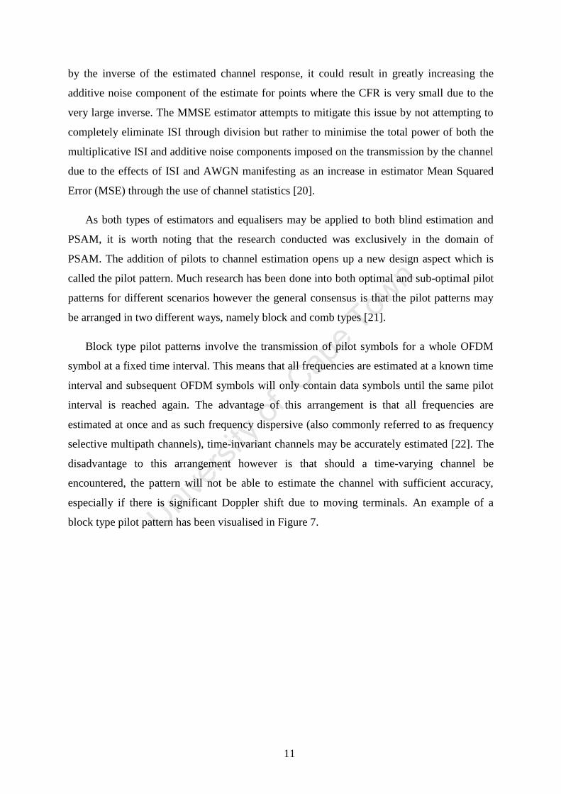
Block type pilot patterns involve the transmission of pilot symbols for a whole OFDM

symbol at a fixed time interval. This means that all frequencies are estimated at a known time

interval and subsequent OFDM symbols will only contain data symbols until the same pilot

interval is reached again. The advantage of this arrangement is that all frequencies are

estimated at once and as such frequency dispersive (also commonly referred to as frequency

selective multipath channels), time-invariant channels may be accurately estimated [22]. The

disadvantage to this arrangement however is that should a time-varying channel be

encountered, the pattern will not be able to estimate the channel with sufficient accuracy,

especially if there is significant Doppler shift due to moving terminals. An example of a

block type pilot pattern has been visualised in Figure 7.

12

Frequency

Time

Figure 7. This figure shows an example pilot arrangement for a block type pilot pattern. The pilot symbols are

denoted by the hatch overlay and a pilot interval of 3 in the time direction is shown.

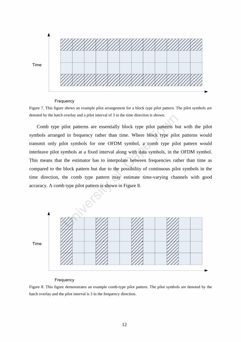
Comb type pilot patterns are essentially block type pilot patterns but with the pilot

symbols arranged in frequency rather than time. Where block type pilot patterns would

transmit only pilot symbols for one OFDM symbol, a comb type pilot pattern would

interleave pilot symbols at a fixed interval along with data symbols, in the OFDM symbol.

This means that the estimator has to interpolate between frequencies rather than time as

compared to the block pattern but due to the possibility of continuous pilot symbols in the

time direction, the comb type pattern may estimate time-varying channels with good

accuracy. A comb type pilot pattern is shown in Figure 8.

Frequency

Time

Figure 8. This figure demonstrates an example comb-type pilot pattern. The pilot symbols are denoted by the

hatch overlay and the pilot interval is 3 in the frequency direction.

13

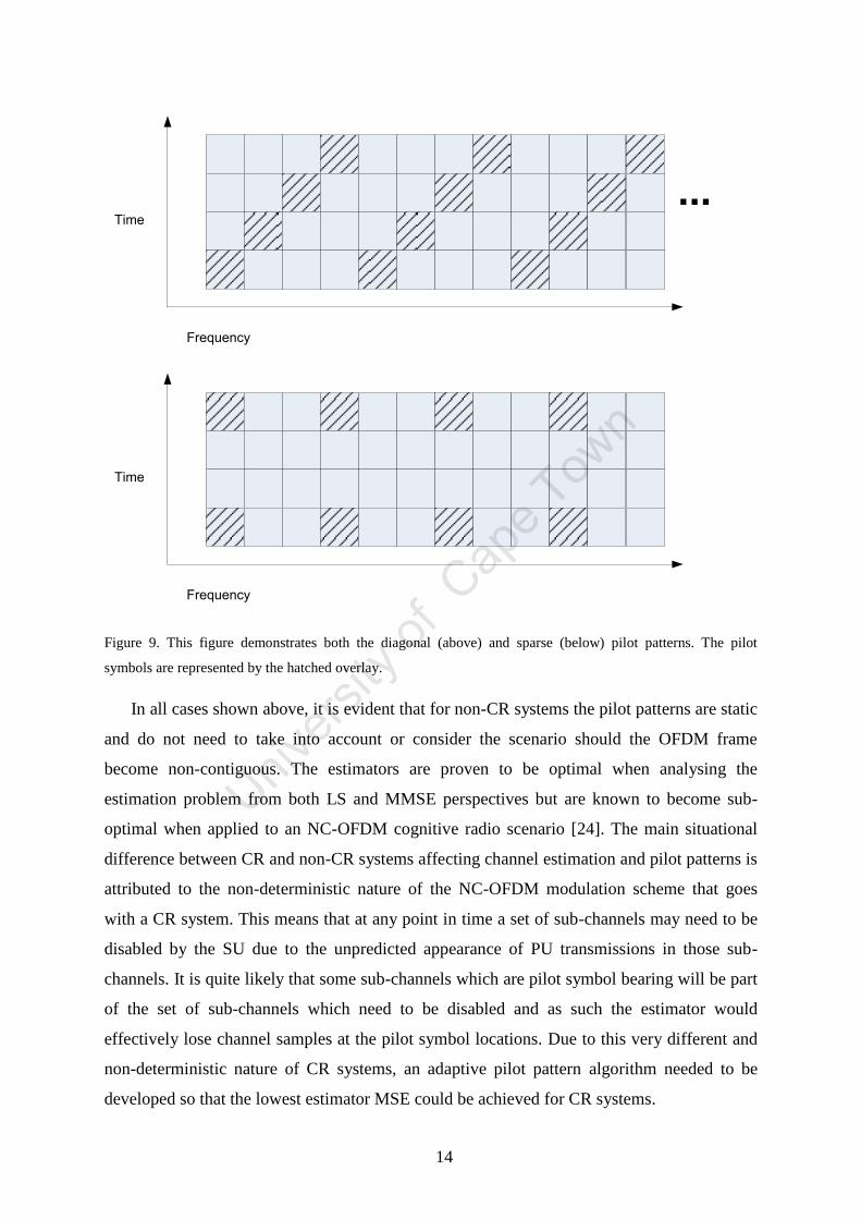
As of recently, there exist a third type of pilot pattern which is a combination of both,

these are usually known as diagonal or scattered pilot patterns. The design of these pilot

patterns is not aimed at a fixed pattern as is with block and comb type but rather with the

estimation accuracy for the most commonly used application scenarios. As such, many

standards such as DVB-T2 [23] employ rectangular patterns where the pilot symbols are

either arranged at a fixed frequency interval similar to comb type but with the interval not

being a multiple of the OFDM symbol length. This essentially results in the pilot symbols

shifting or drifting along the OFDM frame to provide a compromise of the frequency-

dispersive channel estimation accuracy of block arrangements with the time-variant channel

estimation accuracy of comb arrangements. Another commonly employed variation is a

sparse pilot pattern. This pattern is employed especially for low-mobility, high rate

applications and involves the pilot symbols being arranged at an interval in both the time and

the frequency domain so as to minimize the overhead caused by the introduction of known

symbols (pilots) into the OFDM frame.

14

Frequency

Time

Frequency

Time

...

Figure 9. This figure demonstrates both the diagonal (above) and sparse (below) pilot patterns. The pilot

symbols are represented by the hatched overlay.

In all cases shown above, it is evident that for non-CR systems the pilot patterns are static

and do not need to take into account or consider the scenario should the OFDM frame

become non-contiguous. The estimators are proven to be optimal when analysing the

estimation problem from both LS and MMSE perspectives but are known to become sub-

optimal when applied to an NC-OFDM cognitive radio scenario [24]. The main situational

difference between CR and non-CR systems affecting channel estimation and pilot patterns is

attributed to the non-deterministic nature of the NC-OFDM modulation scheme that goes

with a CR system. This means that at any point in time a set of sub-channels may need to be

disabled by the SU due to the unpredicted appearance of PU transmissions in those sub-

channels. It is quite likely that some sub-channels which are pilot symbol bearing will be part

of the set of sub-channels which need to be disabled and as such the estimator would

effectively lose channel samples at the pilot symbol locations. Due to this very different and

non-deterministic nature of CR systems, an adaptive pilot pattern algorithm needed to be

developed so that the lowest estimator MSE could be achieved for CR systems.

15

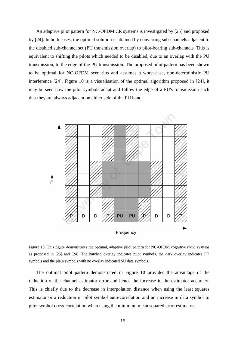
An adaptive pilot pattern for NC-OFDM CR systems is investigated by [25] and proposed

by [24]. In both cases, the optimal solution is attained by converting sub-channels adjacent to

the disabled sub-channel set (PU transmission overlap) to pilot-bearing sub-channels. This is

equivalent to shifting the pilots which needed to be disabled, due to an overlap with the PU

transmission, to the edge of the PU transmission. The proposed pilot pattern has been shown

to be optimal for NC-OFDM scenarios and assumes a worst-case, non-deterministic PU

interference [24]. Figure 10 is a visualisation of the optimal algorithm proposed in [24], it

may be seen how the pilot symbols adapt and follow the edge of a PU's transmission such

that they are always adjacent on either side of the PU band.

P D P PU PU P D PD D

Frequency

Tim

e

Figure 10. This figure demonstrates the optimal, adaptive pilot pattern for NC-OFDM cognitive radio systems

as proposed in [25] and [24]. The hatched overlay indicates pilot symbols, the dark overlay indicates PU

symbols and the plain symbols with no overlay indicated SU data symbols.

The optimal pilot pattern demonstrated in Figure 10 provides the advantage of the

reduction of the channel estimator error and hence the increase in the estimator accuracy.

This is chiefly due to the decrease in interpolation distance when using the least squares

estimator or a reduction in pilot symbol auto-correlation and an increase in data symbol to

pilot symbol cross-correlation when using the minimum mean squared error estimator.

16

1.5. Research Statement and Goals

A number of research questions were initially posed which led to the identification of a

unique problem combining the areas of pilot patterns and power loading for cognitive radios.

These questions are described in detail in Section 1.5.1.

The questions initially posed were refined and a solution was proposed along with the

requirements needed to develop a practical solution which could be implemented successfully

and efficiently. This is described in Section 1.5.2.

An investigation was then done regarding the existence of any solution to the proposed

problem. The results were described in Section 1.5.3.

Finally, the thesis contributions are outlined in detail in Section 1.5.4 with the research

methodology used to derive said contributions described in Section 1.5.5.

1.5.1. Research questions

During the initial stages of the research work, an extensive literature study was

conducted. Several questions were posed as to the possible implementations of cognitive

radio devices in the future. It was then discovered that two of the main aspects needed for a

successful implementation, namely power loading and pilot patterns, turned out be, upon

further investigation, contradictory research findings.

It was noted that research done into optimal power loading algorithms for NC-OFDM

cognitive radios did not consider or differentiate between different symbol types, i.e. pilot or

data, and instead considered all symbols to be of the same type and with the same

requirements. This was found to be a very interesting omission especially after factoring into

account previously investigated research regarding the optimisation of the PDPR in OFDM

based systems. As explained in later sections, in many practical situations the PDPR is

greater than unity. This means that more often than not, the amount of power loaded to a pilot

symbol will be greater than the amount of power loaded to data symbols.

When the literature review on optimal pilot patterns for NC-OFDM CR systems was

conducted, it was found that the aspects of power loading and pilot patterns become

contradictory when needing to be implemented in an NC-OFDM cognitive radio system. This

is due to the fact that the work concerning optimal pilot patterns states that to achieve the

17

lowest estimator MSE, the sub-channels next to PUs should be converted to pilot-bearing

sub-channels to allow compensation for edge effects due to the PU. This however clashes

with research conducted into optimal power loading as in the research it is stated that the

closer a sub-channel is to a PU, the less power it should have allocated to it such that

interference to the PU may be kept under control as well as to compensate for the reduced

channel quality due to PU-to-SU interference. This meant that should the optimal pilot

pattern algorithm and optimal power loading algorithm both be implemented, it would be

necessary to place the pilots at the worst possible positions in terms of SNR so as to improve

the channel estimate, or conversely to place the pilots with their higher power loading

requirements adjacent to the PU and as such creating high SU-to-PU interference and more

than likely going above the design interference threshold.

The identified contradiction was then documented in the research proposal for the project

along with a set of research questions of which the purpose was to be addressed as the

outcome of the research conducted. The research questions were as follows:

Do any solutions exist for the identified contradiction?

For which situations does the contradiction exist?

Are there any special cases where the contradiction does not exist or apply and

how often do they occur?

How can the optimal solution be described mathematically?

How does the solution differ between 1-dimensional and 2-dimensional pilot

patterns?

Are there any sub-optimal schemes or can any be developed?

1.5.2. Requirements of proposed solution

In order to properly develop the solution to the identified problem, several requirements

needed to be outlined such that the problem could be addressed efficiently as well as to make

sure that the solution was well developed for both ideal-case and practical-case

implementations.

The requirements of the outlined solution were as follows:

18

A general solution needed to be developed which could be modified by simple

substitution of heuristic functions or formulae depending on the implementation

scenario.

The solution had to consider both LS and MMSE estimators as they were deemed

to be the most commonly used and both provided unique advantages and

disadvantages in implementation.

The optimal solution needed to consider both 1-dimensional and 2-dimensional

pilot pattern arrangements such that it could be used to optimise a single OFDM

symbol at a time (1-dimensional) or a whole OFDM frame (2-dimensional).

The computational time of the optimal solution would be analysed and a sub-

optimal solution would be proposed.

1.5.3. Comparison to current solutions

With any problem it was necessary to investigate whether it had been previously solved.

As such an extensive literature study was done in the initial stages of the research duration in

order to find whether any solutions to the identified problem were published in online

databases. As of the time of writing, no solutions were found concerning the problem

specification or even the identified contradiction. It was therefore impossible to compare the

solution proposed by this research to any existing solutions due to the fact that no solutions

other than the one proposed in this thesis were found.

It is was however expected that the solution to the identified problem would dictate a

different pilot pattern and pilot symbol placement due to the immense effect the power

loading algorithm has on the estimator MSE. And therefore, it was expected that in many

cases, the optimal pilot position for the new pilot symbol as specified by [24] would actually

not be the proposed optimal pilot symbol placement position. This was due to the fact that the

optimal pilot pattern proposed by [24] dictates that the dynamic pilot symbols be placed

adjacent to the PU transmission bands. These sub-channels however experience great

amounts of PU-to-SU interference and also cause significantly large amounts of SU-to-PU

interference due to their close proximity to the PU. As such, the power loading conditions of

these sub-channels will be really poor due to the optimal power loading algorithm's

interference control purpose. The expectation was that the new optimal pilot symbol position

would actually be a few sub-channels farther from the PU rather than adjacent to it.

19

1.5.4. Thesis Contributions

The contributions of this thesis may be listed and described as follows:

The identification and modelling of the contradiction between optimal pilot

patterns and optimal power loading algorithms for NC-OFDM cognitive radios.

The proposal of an optimal solution method to the contradiction so that the two

necessary algorithms may be optimally applied together.

A generalised solution algorithm is also developed and presented so that the

implementation of the solution is identical between for implementations using

different channel estimators.

Heuristic functions were developed for use with the generalised solution

algorithm so that they may interchangeably be used for either the optimal or sub-

optimal solution.

The computational complexity of the proposed solution algorithm was

investigated, leading to the development of a sub-optimal version of the solution

algorithm which sacrifices accuracy for computational speed.

1.5.5. Research Methodology

Due to the theoretical nature of the problem identified and addressed by the proposed

research topic, the research methodology focused on theoretical and simulation-based data

instead of empirical, measured data.

The research, being theoretical in nature, involved a large portion where theoretical

aspects and solutions were considered. For these situations, the simplifications and reductions

of equations were performed either by hand or utilising Wolfram Mathematica to obtain the

symbolic, simplified solutions.

For simulating the proposed solutions using realistic system parameters, the MATLAB

numerical computation package was used in conjunction with the provided Communication

Tools blockset and functions. The data obtained from simulations were repeated for 10 000

runs such that a statistically significant sample size was obtained and an average was

performed to derive the finalised figures such as MSEs and error function values.

20

1.6. List of Publications

[P1] B. V. Soubachov, N. Ventura, “Contradictions in Power Loading and Pilot Patterns

in NC-OFDM Cognitive Radio Systems”, in proceedings of the Southern Africa

Telecommunication Networks Applications Conference (SATNAC), September 2010.

[P2] B. V. Soubachov, N. Ventura, “Optimal Pilot Placement in Cognitive Radio Systems

for Wiener Filtered MMSE Channel Estimation”, in proceedings of the First

International Conference on Advances in Cognitive Radio (COCORA), April 2011.

[P3] B. V. Soubachov, N. Ventura, “Two-Dimensional, Optimal Pilot Patterns and

Optimal Power Loading in Cognitive Radios”, accepted for the Southern Africa

Telecommunication Networks Applications Conference (SATNAC), September 2011.

[P4] B. V. Soubachov, N. Ventura, “Optimal Pilot Patterns Considering Optimal Power

Loading for Cognitive Radios in the Two Dimensional Scenario”, in the proceedings of

International Telecommunication Union Kaleidoscope (ITU Kaleidoscope), December

2011.

[P5] B. V. Soubachov, N. Ventura, "Optimal Pilot Patterns Using Optimal Power Loading

for NC-OFDM Cognitive Radios", submitted to the Elsevier Journal of Computer

Networks, July 2013.

21

1.7. Thesis Structure

The structure of this thesis is segmented into four major sections. The section layout and

content is described as follows.

Section 1 describes a summary of the literature review conducted during the duration of

research. The section aims to provide an introduction and serve as a primer on multi-carrier

modulation systems, cognitive radio systems as well as the main research fields of concern in

NC-OFDM cognitive radio systems.

Section 2 contains an analysis of the current state of the art and research work done with

relevance to the basics research problem identified in Section 1. This is of specific interest as

it describes the basics needed to understand the research problem as well as a thorough

description as to how and why the identified research problem has arisen.

Section 3 describes the system and mathematical models used to model the problem as

well as in developing the solutions to the identified problem. Section 3.1 describes the

mathematical models as well as the signal processing chain used for OFDM transmissions.

The section also gives a mathematical description of how ISI is mitigated through the use of

low-rate, orthogonal sub-carriers. Section 3.2 elaborates the models used for describing and

analysing the transmission channel as well as the interference between PU and SU

transmissions.

Section 4 describes the optimal solution developed for the stated problem. The section

includes the optimal solution for both LS and MMSE estimators in both the 1-dimensional

and 2-dimensional pilot pattern scenarios. The section also describes the computational run

time complexity analysis of the proposed optimal algorithm as well as methods to reduce

computational complexity through sub-optimal methods.

Section 5 describes the simulation methodology which allowed the solution devised as

part of the research to be modelled and simulated so that evaluations of its performance could

be conducted. The section also describes the parameters used to simulate practical

implementations of the proposed solutions as well as motivating the use of said simulation

parameters. Lastly, Section 5 shows the results obtained from running the simulations to test

the proposed solution to the identified problem, allowing the reader to observe to what extent

the proposed solution requirements were met. There is also a detailed discussion and

22

interpretation of the demonstrated results so that the reader is aided in understanding the way

the problem is solved by the proposed solution as well as to quantify the improvements which

the proposed solution may bring upon future implementations of cognitive radio systems.

Section 6 contains several conclusions about the results stemming from the optimal

algorithms developed in this research work. There is also a discussion on what the practical

implications of this research are and a general conclusion on the work done. A few

suggestions are also mentioned in Section 6 as to what topics could be addressed in future

research work in order to expand and improve the identified problem as well as the problem

solutions developed during the period of the research presented in this thesis.

Lastly, there is a section containing appendices of work used and described in the

sections preceding them. The purpose of the appendices is to describe in detail concepts

mentioned in the preceding sections which were deemed important but did not warrant or

require explicit, detailed explanation and/or derivation. The appendices serve to allow the

reader a better understanding of how the concepts relied upon by this research are derived so

that the way in which the research documented in this thesis uses these concepts as well as

their properties/implications may be better understood.

23

2. Background

This chapter focuses on describing the current advances and progress as well as the state-

of-the-art in NC-OFDM based cognitive radio systems. There is specific focus on how the

origins of multi-carrier modulation have advanced the current data transfer speed capabilities

of modern communications systems as well as why this has become a problem in terms of the

rising demand for ever-increasing speed and accessibility.

2.1. Single/Multi-Carrier Modulation and the Shannon Limit

As the boundaries are ever pushed for higher transmission rates, the impediments caused

by factors such as the channel and noise are more prevalent and are in fact the limiting factors

to the information rates possible by communications systems.

The first wireless communications used were based on the simple principle of single-

carrier modulation. This meant that a modulating signal containing the information required

to be transmitted would modulate a carrier signal at a desired pass-band frequency. This

signal would then be transmitted by the transmitter over a channel or medium with certain

effects imposed on the signal by the channel. The signal would then be received by the

receiver and consequently the modulating signal would be extracted from the modulated

signal through the removal of the carrier. While this approach works for low-rate

transmissions where the signal bandwidth is less than the channel coherence bandwidth,

when the transmitted signal bandwidth is greater than the channel's coherence bandwidth,

inter-symbol interference (ISI) occurs. It is this ISI that is one of the major impediments to

modern communications systems due to the high-rate nature of the information needing to be

transmitted.

Today there are still many communications systems which apply the principles of single-

carrier modulation. These usually tend to be systems where a high data rate is not required

but rather in applications where a low passband bandwidth is required as well as simple

transmitter/receiver implementations.

One of the most common uses of single-carrier modulation is in the analogue

broadcasting of terrestrial television. Television broadcasts are divided into two, differently

24

modulated signals. The video signal performs Amplitude Modulation (AM) on the desired

carrier while the audio signal is Frequency Modulated (FM) on an adjacent carrier at a

frequency higher than the video signal carrier [2]. Both of these methods are considered to be

of a single-carrier modulation type where in the AM modulation (a type of linear modulation)

sense the baseband signal is simply multiplied by the carrier signal to obtain the final,

modulated signal shifted to the desired passband frequency. More specifically, the signal

itself actually undergoes a special type of AM known as Vestigial Sideband Modulation

(VSB). VSB is in itself a special case of Single-Sideband Modulation (SSB) where it has the

same property of having only one side-band transmitted in the passband as SSB but with

VSB the sideband is only partially suppressed and a small vestige of the second sideband also

exists. This allows the passband signal to utilise approximately the same bandwidth when

modulated but is notably susceptible to the noise effects introduced to it by the transmission

channel. The audio signal however is used to modulate the frequency of a carrier instead of

its amplitude as in AM. This means that frequency modulation (a type of non-linear

modulation) allows a much higher resilience to the noise imposed on it by the channel but at

the expense of a greatly increased passband bandwidth.

These characteristics of AM and FM therefore provide a trivial explanation into their

choice for modulating the different signals. The much greater baseband bandwidth of video

signals necessitates that AM modulation be used due to the fact that enormous frequency

bands would be required were it to be frequency modulated. On the other hand, the audio

signal is of a relatively low baseband bandwidth and may therefore exploit the greatly

increased noise resilience of FM at the expense of increased passband bandwidth due to the

much smaller effect it would have.

As of recent, there has been a revival of single-carrier systems for the purposes of high

data rates. In particular, Single Carrier Frequency Division Multiplexing (SC-FDMA) is a

method in which the standard OFDM system is precoded by a Discrete Fourier Transform

(DFT) [3]. The main purpose behind the use of SC-FDMA is that OFDM-based systems tend

to have a very high Peak-to-Average Power Ratio (PAPR) due to the individual modulation

of sub-carriers [4]. The result of this high PAPR translates to an increase in the power

consumption in power amplifier electronics in the device due to their finite linearity. The

high PAPR also results in a loss of fidelity in the amplifiers' output due to the region of non-

linearity at the extreme ends of the amplifier's gain/transfer function causing a phenomenon

known as clipping or saturation [4]. This means that the SC-FDMA scheme is a great

25

replacement for OFDMA in scenarios where the terminal used has a limited source of power.

The most common scenario for this is in mobile telephone user equipment where the phone is

limited by a finite battery life and as such needs to have an energy efficient method of

transmitting information back to the base station. It is because of this property of SC-FDMA

that the modulation scheme has become a part of the next-generation Long Term Evolution

(LTE) cellular communications standard as formed by the 3rd

Generation Partnership Project

(3GPP) [5] in defining the modulation scheme for transmission from the user terminal to the

base station governing the cell.

In order to combat the ISI created by most practical channels, the one major development

which has had the most profound effect is the utilisation of multi-carrier modulation. Instead

of transmitting a single, high-rate (and hence high-bandwidth) modulating signal on a single

carrier, the modulating signal is divided into several, low-rate signals which modulate the

same amount of sub-carriers. This means that instead of having one channel experiencing

frequency-selective fading, which in turn is difficult to equalise, the data are transmitted

through the use of many, lower bandwidth sub-channels which individually experience flat

fading and are therefore much easier to equalise.

As the Shannon limit is achieved only when there are no ISI components present in the

system and only an Additive White Gaussian Noise (AWGN) component remains as an

impediment to the system, it means that through the removal of the ISI a communications

system's information rate may approach, and ideally achieve, the Shannon limit. However, in

order to achieve an ISI-free transmission, many aspects need to be exactly ideal between the

transmitter and receiver, such as the synchronization for the signal centre frequency. While

this may be practically achieved, it will not be a perfect synchronization as some small error

will always exist due to oscillator drift, phase noise and other real-world imperfections. In

practise though, these errors and imperfections tend to be very small and there are many

designs which factor in these imperfections and mitigate them, resulting in very good rates,

albeit not ideal, of ISI mitigation and cancellation.

Due to the significant advantages of multi-carrier systems described above (the main one

being ISI mitigation for a relatively low computational complexity increase) many modern

communications systems have adopted Multi-Carrier (MC) modulation as the modulation

scheme of choice. These systems tend to be prevalent in situations where large data rates are

required and design complexity constraints are not as severe. It is therefore evident that these

26

situations tend to be more complex systems such as IEEE 802.11 (WiFi) and next-generation

cellular phone standards like LTE.

The most widely-spread example of the successful application of MC modulation (and

OFDM in specific) is the IEEE 802.11a/g/n (WiFi) standards for Wireless Local Area

Networks (WLAN). In the three standards, the most widely used one is the IEEE 802.11g

standard. It defines a modulation scheme where a 20 MHz channel is divided by an OFDM

MC modulation scheme with the channel divided into 64 sub-channels, each with a sub-

channel bandwidth (equivalent to sub-carrier spacing due to the orthogonality of OFDM) of

312.5 kHz. [6]. The small number of sub-channels and the large sub-channel bandwidth lead

to a very resilient modulation configuration in terms of the ability to handle time-variance in

the transmission channel. The ease with which equalisation may be performed once moved

from the time to the frequency domain by the use of OFDM has also shown to be a major

deciding factor in the formulation of the standard. These immense increases in efficiency

have contributed greatly to the success and adoption of IEEE 802.11 as the de facto standard

for consumer-grade, wireless local area networks. The latter iterations of IEEE 802.11

(specifically, IEEE 802.11g) allow the system to conduct transmissions with data rates such

as 54 Mbit/s in a passband bandwidth of 20 MHz [6].

However, there are also many examples where the IEEE 802.11 standard has been

successfully repurposed for use in long-range, outdoor transmission systems. The most

notable example of the adoption of IEEE 802.11 for long-range, outdoor transmissions is

Wireless Internet Service Providers (WISPs). While this use is contrary to the design

purposes of the IEEE 802.11 standard, its efficiency and resilience as well as its low-price

hardware due to its large-scale adoption for indoor WLANs mean that it has become a very

popular choice for transmission hardware in WISP situations.

Another very important use of OFDM is in the design and drafting of the Digital Video

Broadcast (DVB) standard destined as the replacement modulation scheme (DVB-T & DVB-

T2 specifically) for current, analogue terrestrial television transmissions as discussed a few

paragraphs earlier. The most recent version of the DVB standard for terrestrial broadcasts is

the second iteration, known as DVB-T2., which is designed for the transmission (broadcast)

of very high data rate information such as high-definition video. This means that the

modulation scheme needs to be able to support these high data rates while also providing

27

resilience to the effects imposed by the channel due to the very large areas covered by the

broadcast transmitter.

Due to the high information content present in the main use purpose of DVB-T2, the

standard needed to support high data rates comparable to the ones provided by IEEE 802.11g

while making use of even smaller passband bandwidths due to the traditional analogue

terrestrial television transmissions making use of 8 MHz channels for broadcast [2]. DVB-T2

was therefore developed to be even more spectrally efficient than IEEE 802.11g and, on two

extremes, provides data rates as high as of 45.24 Mbit/s while utilising a maximum passband

bandwidth of 10 MHz with an FFT size ranging anywhere from 1K (1024) to 32K (32768)

[7]. This means that DVB-T2 presents an even higher increase in spectral efficiency, further

enforcing the practical utility of OFDM transmission.

The ubiquitous popularity of OFDM has however not only been limited to wireless

applications. OFDM modulation has been successfully used for wired, digital data

transmissions over the standard telephone lines which are used simultaneously for analogue

voice in many homes. This technology is commonly known as Digital Subscriber Line (DSL)

such that the telephone line in the Plain Old Telephone Service (POTS) is utilised to the

extent that any higher frequencies than the baseband (used for voice) are used for the

transmission and reception of digital data. In the wired scenario, the OFDM modulation

scheme is referred to Discrete Multitone (DMT) modulation which forms the core of the ITU

G.992.1 (also known as G.DMT) standard. The G.DMT standards achieve high-data rates

over the wired channel by utilising OFDM modulation to divide the upper frequency band

(25+ kHz) above the POTS baseband (0-4 kHz) into a large number of orthogonal bins (sub-

channels). This allows G.DMT devices to achieve data rates of up to 8 Mbit/s [8]. Further

improvements have resulted in the formation of ADSL2 and ADSL2+ standards which allow

downstream rates as high as 24 Mbit/s using the same telephone copper line.

In many countries, DSL has been the technology of choice for providing high-speed

broadband with the fixed-price, always-on capability not traditionally present in legacy, dial-

up systems. This technology has allowed for the dramatic increase in the broadband

penetration of many countries due to its very high data rates as well as the fact that the

infrastructure needed for its proliferation (the analogue, telephone service) was already

available in most countries. In order for service providers to provide a DSL service, the only

requirements were that the subscriber has the necessary Consumer Premises Equipment

28

(CPE) on their service (usually a modem and router integrated into one unit) and that the

service provider installs Digital Subscriber Line Access Multiplexers (DSLAMs) on the other

end of the local loop. This meant that no new infrastructure needed to be rolled out other than

installing DSLAMs on street-level cabinets which served tens of users at once. The price of

providing a DSL service was therefore of a significantly low cost when compared to

alternative access methods at the time of its introduction. This led to the technology

becoming widely adopted for the provision of broadband internet access to both homes and

businesses [9].

The great advantage of OFDM almost completely mitigating ISI has proven to be popular

also in its extension to the multiple-access scenario. Orthogonal Frequency Division Multiple

Access (OFDMA) is a technique that is essentially identical to OFDM with the major

exception that instead of using all sub-channels for the transmission between two devices,

sets of sub-channels may be assigned to different devices and as such different data may be

transmitted to multiple devices at the same time through the independent use of different

frequencies. This therefore allows highly efficient multiple-access communication systems to

be implemented utilising the minimum amount of spectrum possible due to the orthogonality

of the sub-channels allowing for transmissions without any guard bands in between the sub-

channels themselves. The naming conventions used when describing OFDM-based

modulation systems are described in Figure 11 below.

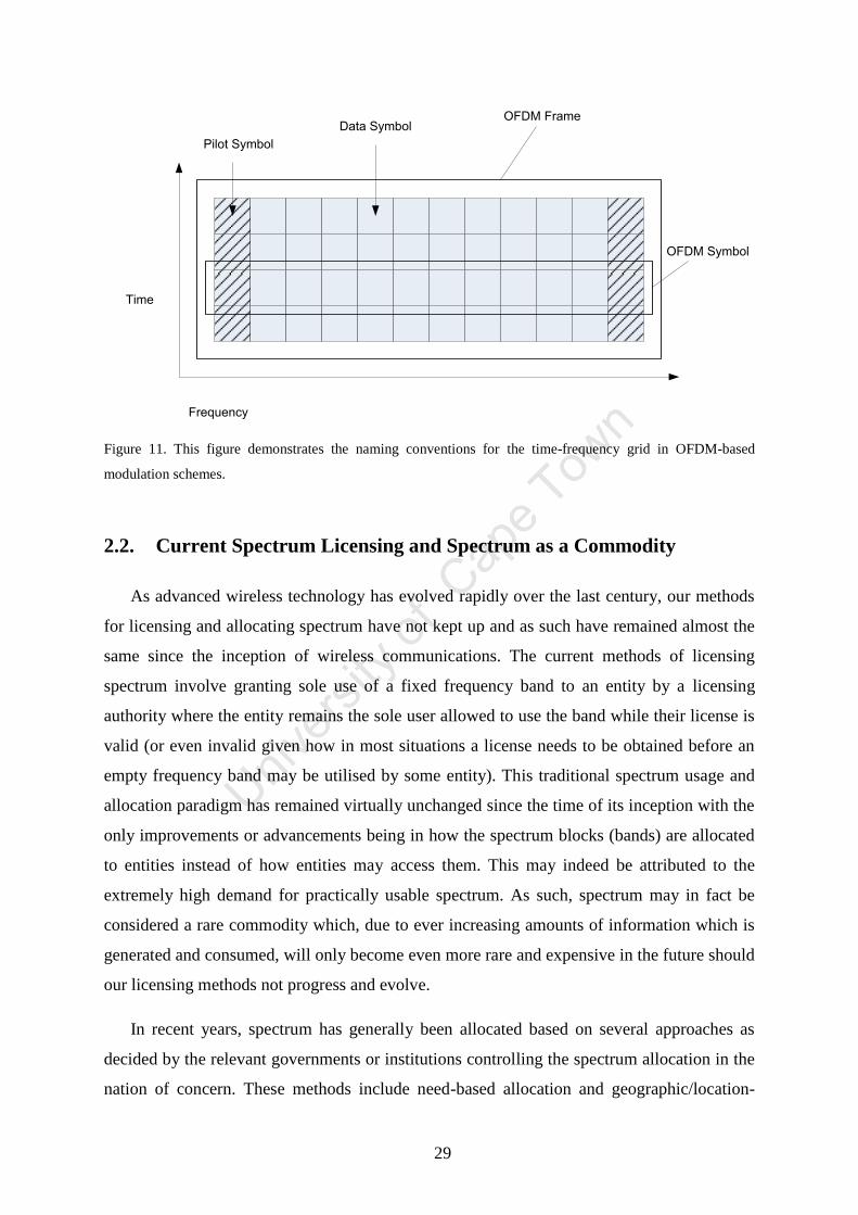
29

Frequency

Time

Data Symbol

Pilot Symbol

OFDM Frame

OFDM Symbol

Figure 11. This figure demonstrates the naming conventions for the time-frequency grid in OFDM-based

modulation schemes.

2.2. Current Spectrum Licensing and Spectrum as a Commodity

As advanced wireless technology has evolved rapidly over the last century, our methods

for licensing and allocating spectrum have not kept up and as such have remained almost the

same since the inception of wireless communications. The current methods of licensing

spectrum involve granting sole use of a fixed frequency band to an entity by a licensing

authority where the entity remains the sole user allowed to use the band while their license is

valid (or even invalid given how in most situations a license needs to be obtained before an

empty frequency band may be utilised by some entity). This traditional spectrum usage and

allocation paradigm has remained virtually unchanged since the time of its inception with the

only improvements or advancements being in how the spectrum blocks (bands) are allocated

to entities instead of how entities may access them. This may indeed be attributed to the

extremely high demand for practically usable spectrum. As such, spectrum may in fact be

considered a rare commodity which, due to ever increasing amounts of information which is

generated and consumed, will only become even more rare and expensive in the future should

our licensing methods not progress and evolve.

In recent years, spectrum has generally been allocated based on several approaches as

decided by the relevant governments or institutions controlling the spectrum allocation in the

nation of concern. These methods include need-based allocation and geographic/location-

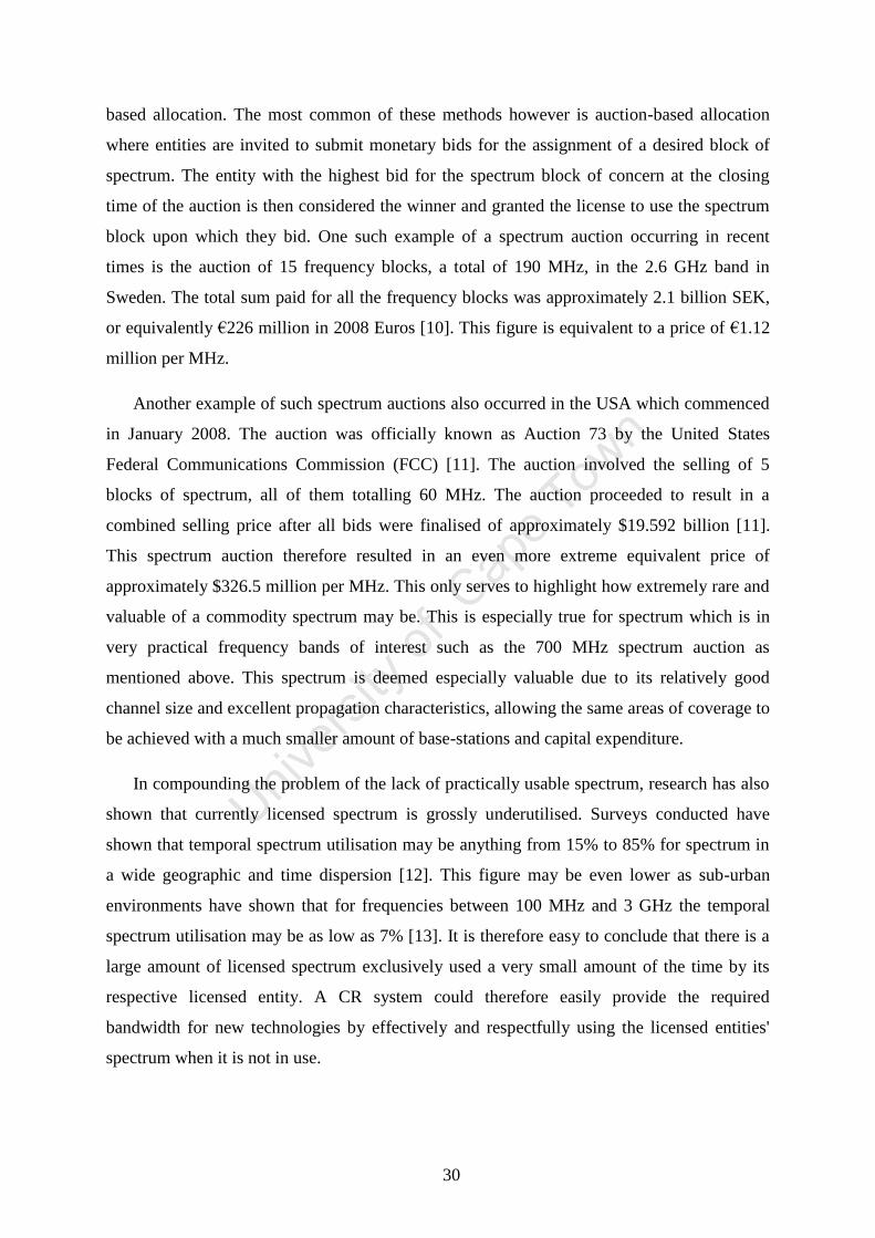
30

based allocation. The most common of these methods however is auction-based allocation

where entities are invited to submit monetary bids for the assignment of a desired block of

spectrum. The entity with the highest bid for the spectrum block of concern at the closing

time of the auction is then considered the winner and granted the license to use the spectrum

block upon which they bid. One such example of a spectrum auction occurring in recent

times is the auction of 15 frequency blocks, a total of 190 MHz, in the 2.6 GHz band in

Sweden. The total sum paid for all the frequency blocks was approximately 2.1 billion SEK,

or equivalently €226 million in 2008 Euros [10]. This figure is equivalent to a price of €1.12

million per MHz.

Another example of such spectrum auctions also occurred in the USA which commenced

in January 2008. The auction was officially known as Auction 73 by the United States

Federal Communications Commission (FCC) [11]. The auction involved the selling of 5

blocks of spectrum, all of them totalling 60 MHz. The auction proceeded to result in a

combined selling price after all bids were finalised of approximately $19.592 billion [11].

This spectrum auction therefore resulted in an even more extreme equivalent price of

approximately $326.5 million per MHz. This only serves to highlight how extremely rare and

valuable of a commodity spectrum may be. This is especially true for spectrum which is in

very practical frequency bands of interest such as the 700 MHz spectrum auction as

mentioned above. This spectrum is deemed especially valuable due to its relatively good

channel size and excellent propagation characteristics, allowing the same areas of coverage to

be achieved with a much smaller amount of base-stations and capital expenditure.

In compounding the problem of the lack of practically usable spectrum, research has also

shown that currently licensed spectrum is grossly underutilised. Surveys conducted have

shown that temporal spectrum utilisation may be anything from 15% to 85% for spectrum in

a wide geographic and time dispersion [12]. This figure may be even lower as sub-urban

environments have shown that for frequencies between 100 MHz and 3 GHz the temporal

spectrum utilisation may be as low as 7% [13]. It is therefore easy to conclude that there is a

large amount of licensed spectrum exclusively used a very small amount of the time by its

respective licensed entity. A CR system could therefore easily provide the required

bandwidth for new technologies by effectively and respectfully using the licensed entities'

spectrum when it is not in use.

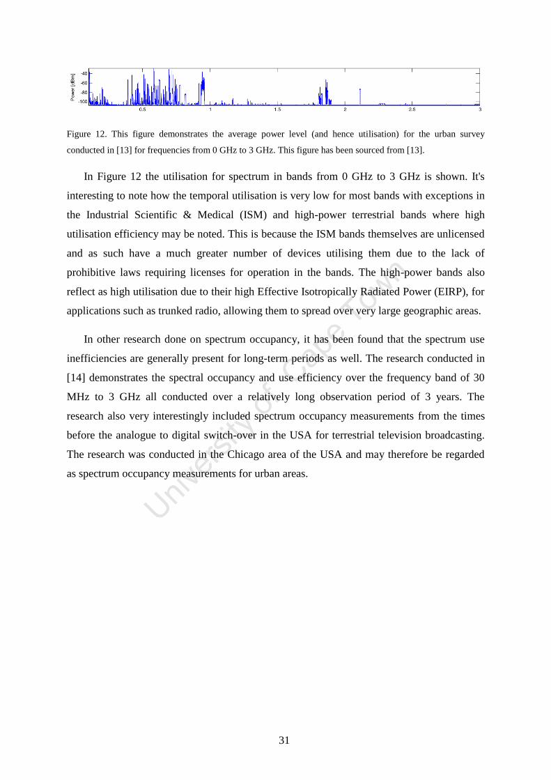
31

Figure 12. This figure demonstrates the average power level (and hence utilisation) for the urban survey

conducted in [13] for frequencies from 0 GHz to 3 GHz. This figure has been sourced from [13].

In Figure 12 the utilisation for spectrum in bands from 0 GHz to 3 GHz is shown. It's

interesting to note how the temporal utilisation is very low for most bands with exceptions in

the Industrial Scientific & Medical (ISM) and high-power terrestrial bands where high

utilisation efficiency may be noted. This is because the ISM bands themselves are unlicensed

and as such have a much greater number of devices utilising them due to the lack of

prohibitive laws requiring licenses for operation in the bands. The high-power bands also

reflect as high utilisation due to their high Effective Isotropically Radiated Power (EIRP), for

applications such as trunked radio, allowing them to spread over very large geographic areas.

In other research done on spectrum occupancy, it has been found that the spectrum use

inefficiencies are generally present for long-term periods as well. The research conducted in

[14] demonstrates the spectral occupancy and use efficiency over the frequency band of 30

MHz to 3 GHz all conducted over a relatively long observation period of 3 years. The

research also very interestingly included spectrum occupancy measurements from the times

before the analogue to digital switch-over in the USA for terrestrial television broadcasting.

The research was conducted in the Chicago area of the USA and may therefore be regarded

as spectrum occupancy measurements for urban areas.

32

Figure 13. This figure demonstrates the spectrum occupancy percentage, analogous to the spectrum temporal

usage efficiency, as conducted by [14] for the year 2008. Extracted from [14].

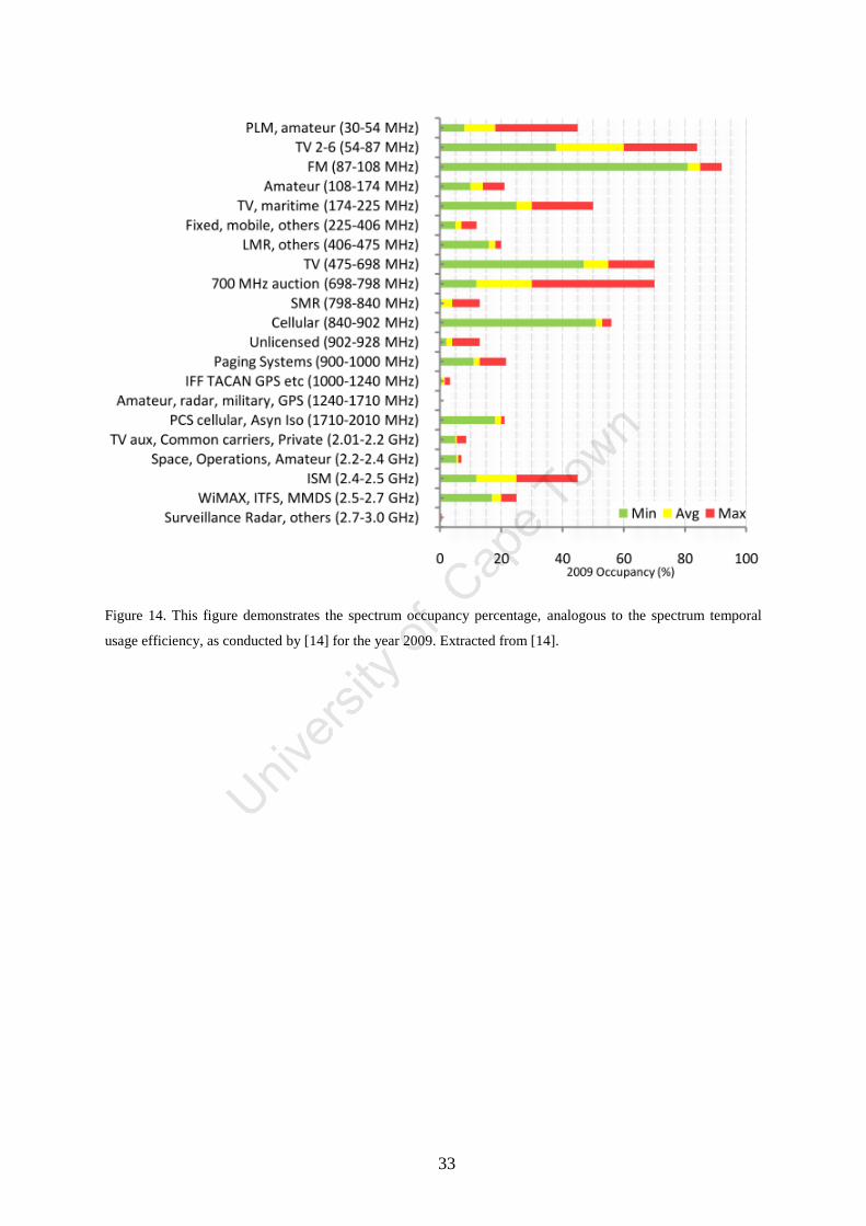
33

Figure 14. This figure demonstrates the spectrum occupancy percentage, analogous to the spectrum temporal

usage efficiency, as conducted by [14] for the year 2009. Extracted from [14].

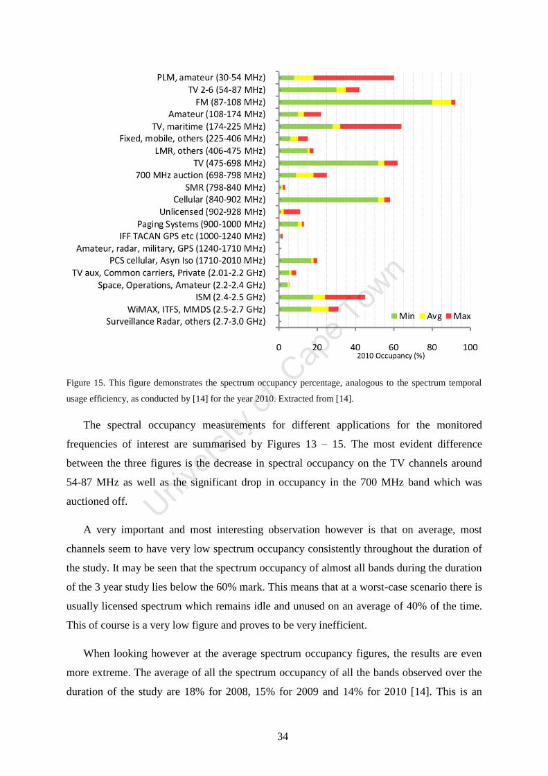
34

Figure 15. This figure demonstrates the spectrum occupancy percentage, analogous to the spectrum temporal

usage efficiency, as conducted by [14] for the year 2010. Extracted from [14].

The spectral occupancy measurements for different applications for the monitored

frequencies of interest are summarised by Figures 13 – 15. The most evident difference

between the three figures is the decrease in spectral occupancy on the TV channels around

54-87 MHz as well as the significant drop in occupancy in the 700 MHz band which was

auctioned off.

A very important and most interesting observation however is that on average, most

channels seem to have very low spectrum occupancy consistently throughout the duration of

the study. It may be seen that the spectrum occupancy of almost all bands during the duration

of the 3 year study lies below the 60% mark. This means that at a worst-case scenario there is

usually licensed spectrum which remains idle and unused on an average of 40% of the time.

This of course is a very low figure and proves to be very inefficient.

When looking however at the average spectrum occupancy figures, the results are even

more extreme. The average of all the spectrum occupancy of all the bands observed over the

duration of the study are 18% for 2008, 15% for 2009 and 14% for 2010 [14]. This is an

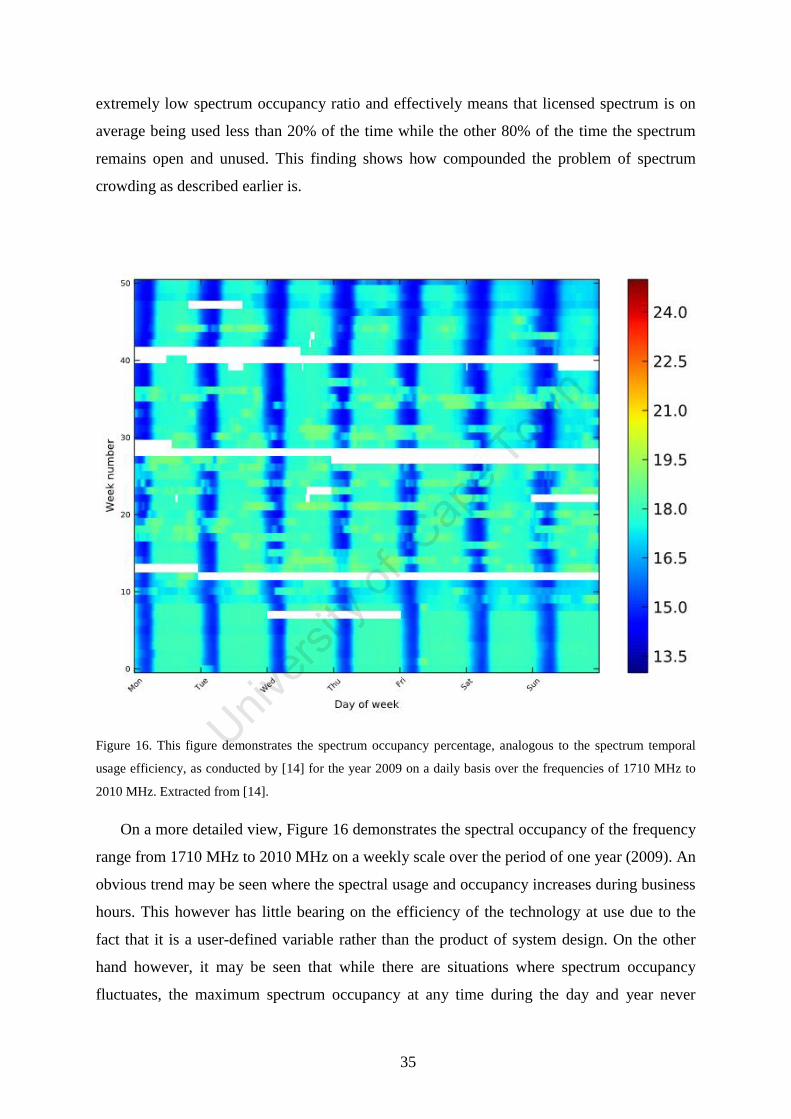
35

extremely low spectrum occupancy ratio and effectively means that licensed spectrum is on

average being used less than 20% of the time while the other 80% of the time the spectrum

remains open and unused. This finding shows how compounded the problem of spectrum

crowding as described earlier is.

Figure 16. This figure demonstrates the spectrum occupancy percentage, analogous to the spectrum temporal

usage efficiency, as conducted by [14] for the year 2009 on a daily basis over the frequencies of 1710 MHz to

2010 MHz. Extracted from [14].

On a more detailed view, Figure 16 demonstrates the spectral occupancy of the frequency

range from 1710 MHz to 2010 MHz on a weekly scale over the period of one year (2009). An

obvious trend may be seen where the spectral usage and occupancy increases during business

hours. This however has little bearing on the efficiency of the technology at use due to the

fact that it is a user-defined variable rather than the product of system design. On the other

hand however, it may be seen that while there are situations where spectrum occupancy

fluctuates, the maximum spectrum occupancy at any time during the day and year never

36

exceeds a value above 21%. This means that even during worst-case usage scenarios, the

current licensing method of single-entity use only for a band of spectrum is still extremely

inefficient due to its result being that there is a huge demand for spectrum in order to allow

new technologies and businesses to emerge but at the same time the licensing frameworks

and methods currently used do not allow these new entities to utilise existing, licensed

spectrum when the spectrum licensees are not using it. As it has been shown that the

licensees are very inefficient in using their spectrum, this could only mean that a great deal of

effective spectrum could be gained by allowing new entities to use the licensed spectrum of

the current licensees when the licensees themselves are not using it.

37

3. System Models

As with the design of any system, NC-OFDM cognitive radio systems may be broken

down into several sub-components. These components as well as the effects imposed on the

transmission need to be modelled correctly such that simulations and appropriate solutions

may be obtained for different usage scenarios and applications.

This chapter introduces the OFDM system model for multicarrier transmissions in more

detail in Section 3.1 and explains the mathematical and practical aspects of it. In Section 3.2

channel and interference models are introduced to the reader such that the effects and

impairments caused during the transmission and reception of signals may be understood.

Section 3.3 introduces the concept of the optimal power loading algorithm for NC-OFDM

CRs which is used to solve interference issues while maximising the transmission rate.

Sections 3.4 & 3.5 then introduce the concept of estimation error for both the LS and MMSE

channel estimators and demonstrate how crucial channel estimation is to obtaining much

higher information transfer rates than would be possible without channel estimation. Section

3.6 then describes the optimal pilot pattern algorithm proposed by previous research which

allows the NC-OFDM cognitive radio system to maximize its information transfer rate by

reducing the channel estimator MSE to be as small as possible.

It should be noted that Sections 3.3 & 3.6 are important aspects for the implementation of

a communications system as both are deemed necessary in modern systems. As such, these

algorithms are central to the research conducted and their combination together in a new

environment/paradigm is in fact the problem addressed by this research.

3.1. OFDM-based System Models

OFDM systems allow for no guard-bands in between the data transmission sub-channels,

which when combined with frequency-domain equalization allow the communications

system to approach the Shannon limit in terms of channel capacity at a specified SNR. The

mathematical description and theory of OFDM modulation as well as its characteristics are

explained in detail in this section. The practical modulation parameters and techniques such

as Cyclic Prefix (CP) are also considered in this section.

38

3.1.1. OFDM modulation theory

An OFDM system needs to be implemented using an orthogonal set of basis functions.

This allows the sub-channel spacing to be exactly the inverse of the symbol duration ( ) and

as such allows for successful transmission and reception without the use of guard-bands in

between every sub-channel. The set of basis functions used for the OFDM system are the

complex multipliers established by the Discrete Fourier Transform (DFT) in the DFT matrix.

The DFT may then be computed as [4]

where is the size DFT transform of the input . The DFT may be more simply

represented by the symbol allowing the DFT to be more easily rewritten as

where denotes the vector or matrix form of the complex input signal x.

The computationally efficient implementation of the DFT, the Fast Fourier Transform

(FFT), may be represented in matrix form where the FFT matrix is calculated based on what

is known as the twiddle factors. The most commonly used FFT algorithm is the Cooley-

Tukey algorithm [4]. As the DFT/FFT matrix is the implementation of a DFT/FFT as matrix

multiplication, the DFT may be represented in matrix space as

and the -size DFT matrix may be computed as [26]

where

∑

(1)

(2)

(3)

[

] (4)

√

(5)

39

The factor shown in (5) above is commonly known as the twiddle factor when

implemented as an FFT and is in fact an root of unity. The division by the normalisation

factor √ is added such that the energy of the output is equivalent to the energy of the input.

A very important aspect about the DFT is that the twiddle factors all form an orthogonal basis

as the inner product of all the twiddle factors is in fact zero.

Using the orthogonality provided by the FFT, we may exploit this to allow modulation of

symbols into multiple, overlapping sub-carriers. This means that the overlapping, out-of-

band, transmissions of the sub-carriers negate each other at the sample points, allowing for a

no guard-band requirement. This then implies that the modulated symbols will be spaced at

exactly the inverse of the symbol duration and therefore allowing maximum utilisation of the

band of operation due to the lack of overhead and inefficiency introduced by guard-bands.

The orthogonality provided by the DFT also allows the Inter-Channel Interference (ICI)

caused by other sub-channels into a given sub-channel to cancel out completely at the exact

centre (integer) sampling point of the sub-channel considered. This property is visualised for

five sub-channels in Figure 17.

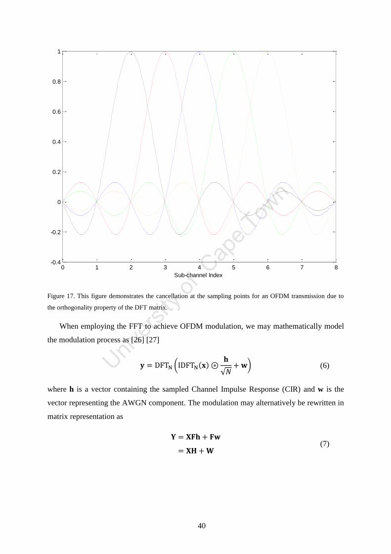
40

Figure 17. This figure demonstrates the cancellation at the sampling points for an OFDM transmission due to

the orthogonality property of the DFT matrix.

When employing the FFT to achieve OFDM modulation, we may mathematically model

the modulation process as [26] [27]

where h is a vector containing the sampled Channel Impulse Response (CIR) and w is the

vector representing the AWGN component. The modulation may alternatively be rewritten in

matrix representation as

0 1 2 3 4 5 6 7 8-0.4

-0.2

0

0.2

0.4

0.6

0.8

1

Sub-channel Index

(

√ ) (6)

(7)

41

where is the channel frequency response vector obtained by the FFT of the channel

impulse response. This allows us to demodulate the received signal by dividing it by the

estimated CFR as

where is the estimation error between the actual CFR and the estimated CFR. It should be

noted that the estimator has some effect on the noise level in the signal after demodulation;

this is explained in detail in Section 3.4.

It may therefore be seen that through the use of the IDFT before transmission and the

DFT after reception, the OFDM modulation converts the transmitted symbols from a

sequence in the time domain to a sequence in the frequency domain. As such, instead of using

the complex Maximum Likelihood Sequence Estimator (MLSE) to estimate the most likely

sequence in which the symbols arrived, the channel ISI effect is converted into the frequency

domain which may be trivially equalised by linear division or multiplication and inversion.

While the orthogonal modulation of OFDM allows us to ideally mitigate the effects of ISI

imposed on the signal completely, it does not however guarantee the mitigation of ICI or ISI

in between OFDM symbols. As such, a technique involving the addition of a cyclic prefix to

the OFDM symbol is necessary. The cyclic prefix involves copying a given amount of sub-

channels of length LCP from the end of the OFDM symbol and prefixing them at the front of

the OFDM symbol. This means that the OFDM symbol length is extended by LCP symbols.

The purpose of this extension is to allow for the channel ISI effects from the previous OFDM

symbol to subside and as such has to be chosen so that the length of LCP is greater than or

equal to the channel delay spread (this concept is explained in detail in Section 3.2). This

means that the OFDM symbol at the current time only receives ISI from itself at the actual

start of the OFDM symbol. [4].

Only using a prefix (or even a suffix) for an OFDM symbol would suffice to combat ISI

between OFDM symbols, however this does not mitigate the effects of ICI. In order to

combat ICI effects, there needs to be specifically a cyclic prefix rather than a null

prefix/suffix. The cyclic prefix allows the convolution performed on the OFDM symbol by

(8)

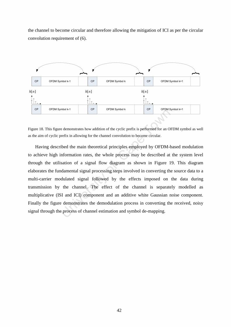
42

the channel to become circular and therefore allowing the mitigation of ICI as per the circular

convolution requirement of (6).

OFDM Symbol k-1CP}

OFDM Symbol kCP

}

OFDM Symbol k+1CP

}

OFDM Symbol k-1CP OFDM Symbol kCP OFDM Symbol k+1CP

][nh ][nh ][nh

Figure 18. This figure demonstrates how addition of the cyclic prefix is performed for an OFDM symbol as well

as the aim of cyclic prefix in allowing for the channel convolution to become circular.

Having described the main theoretical principles employed by OFDM-based modulation

to achieve high information rates, the whole process may be described at the system level

through the utilisation of a signal flow diagram as shown in Figure 19. This diagram

elaborates the fundamental signal processing steps involved in converting the source data to a

multi-carrier modulated signal followed by the effects imposed on the data during

transmission by the channel. The effect of the channel is separately modelled as

multiplicative (ISI and ICI) component and an additive white Gaussian noise component.

Finally the figure demonstrates the demodulation process in converting the received, noisy

signal through the process of channel estimation and symbol de-mapping.

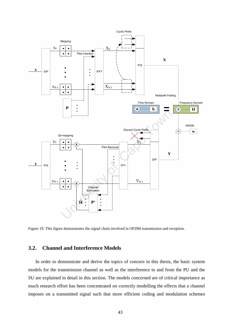
43

S/P

.

. ..

.

. ..

. . .

IFFT

HX

+ w

x

X0

XN-1

P/S

x0

xN-1

X

Y

P

. . .

. . .

P/S

.

. ..

.

. ..

. . .FFT

y

Y0

YN-1

S/P

y0

yN-1

Mapping

Pilot Insertion

Multipath Fading

AWGN

De-mapping

* h

Frequency DomainTime Domain

Cyclic Prefix

Discard Cyclic Prefix

P’

. . .

. . .

. . .

. . .

H

Pilot Removal

Channel

Estimation

X

X

Figure 19. This figure demonstrates the signal chain involved in OFDM transmission and reception.

3.2. Channel and Interference Models

In order to demonstrate and derive the topics of concern in this thesis, the basic system

models for the transmission channel as well as the interference to and from the PU and the

SU are explained in detail in this section. The models concerned are of critical importance as

much research effort has been concentrated on correctly modelling the effects that a channel

imposes on a transmitted signal such that more efficient coding and modulation schemes

44

could be developed. The same applies to research conducted on interference between

different frequency bands, also known as out-of-band or OOB interference, due to the limit of

practically usable spectrum enforcing designers and engineers to minimize guard-bands

between transmission bands to be as small as is absolutely necessary.

3.2.1. Power density spectrum of signals

In order to successfully model interference from transmissions, one has to be able to

obtain the Power Density Spectrum (PDS) of the transmitted signals. The PDS is the measure

of the signal power or energy, depending on the signal type, for all the spectra of a signal.

The PDS is usually described in Watts/Hz or more conventionally dBm/Hz where dBm is the

decibel power measurement relative to one milliwatt. The PDS therefore allows us to model

the signal power for all the spectra and with the sum of the PDS at all spectra providing the

total transmitted power or energy.

As it is assumed that at no point does the CR system have any information about the PUs'

transmissions other than the transmission power, a naïve assumption may then be made by

the SU that the PUs' employ a rectangular pulse-shaping function. This means that the PDS

of a PU transmission will be described as [30] [19]

(

)

(16)

where is the power loaded to the sub-channel and is the symbol duration (i.e. the

inverse of the sub-channel bandwidth).

While the PDS used to model the transmitted signals in the system is one for a

rectangular pulse-shaping function, it may be easily interchanged for the PDS of any pulse-

shaping function required. The PDS of the required function is easily obtainable as the

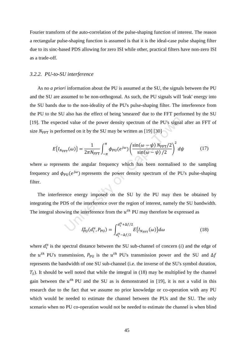
45

Fourier transform of the auto-correlation of the pulse-shaping function of interest. The reason

a rectangular pulse-shaping function is assumed is that it is the ideal-case pulse shaping filter

due to its sinc-based PDS allowing for zero ISI while other, practical filters have non-zero ISI

as a trade-off.

3.2.2. PU-to-SU interference

As no a priori information about the PU is assumed at the SU, the signals between the PU

and the SU are assumed to be non-orthogonal. As such, the PU signals will 'leak' energy into

the SU bands due to the non-ideality of the PU's pulse-shaping filter. The interference from

the PU to the SU also has the effect of being 'smeared' due to the FFT performed by the SU

[19]. The expected value of the power density spectrum of the PU's signal after an FFT of

size is performed on it by the SU may be written as [19] [30]

where represents the angular frequency which has been normalised to the sampling

frequency and represents the power density spectrum of the PU's pulse-shaping

filter.

The interference energy imposed on the SU by the PU may then be obtained by

integrating the PDS of the interference over the region of interest, namely the SU bandwidth.

The integral showing the interference from the PU may therefore be expressed as

where is the spectral distance between the SU sub-channel of concern ( ) and the edge of

the PU's transmission, is the PU's transmission power and the SU and

represents the bandwidth of one SU sub-channel (i.e. the inverse of the SU's symbol duration,

). It should be well noted that while the integral in (18) may be multiplied by the channel

gain between the PU and the SU as is demonstrated in [19], it is not a valid in this

research due to the fact that we assume no prior knowledge or co-operation with any PU

which would be needed to estimate the channel between the PUs and the SU. The only

scenario when no PU co-operation would not be needed to estimate the channel is when blind

{

}

∫

(

)

(17)

∫ { }

(18)

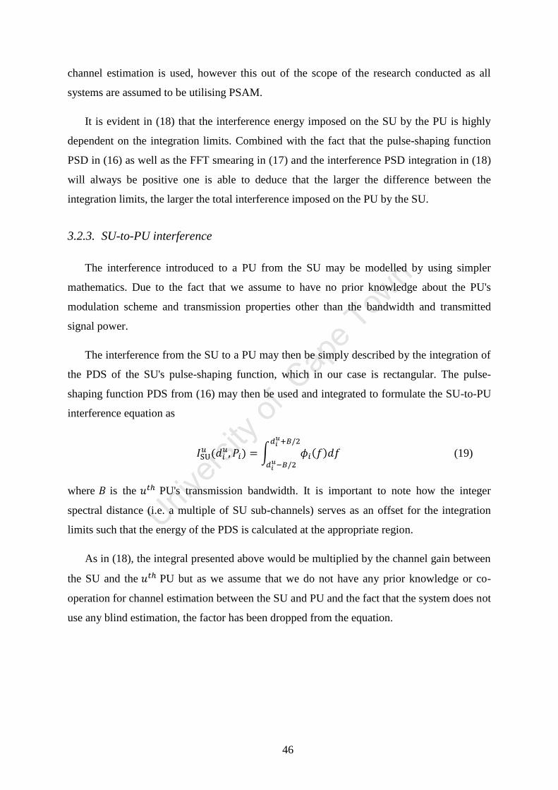
46

channel estimation is used, however this out of the scope of the research conducted as all

systems are assumed to be utilising PSAM.

It is evident in (18) that the interference energy imposed on the SU by the PU is highly

dependent on the integration limits. Combined with the fact that the pulse-shaping function

PSD in (16) as well as the FFT smearing in (17) and the interference PSD integration in (18)

will always be positive one is able to deduce that the larger the difference between the

integration limits, the larger the total interference imposed on the PU by the SU.

3.2.3. SU-to-PU interference

The interference introduced to a PU from the SU may be modelled by using simpler

mathematics. Due to the fact that we assume to have no prior knowledge about the PU's

modulation scheme and transmission properties other than the bandwidth and transmitted

signal power.

The interference from the SU to a PU may then be simply described by the integration of

the PDS of the SU's pulse-shaping function, which in our case is rectangular. The pulse-

shaping function PDS from (16) may then be used and integrated to formulate the SU-to-PU

interference equation as

where is the PU's transmission bandwidth. It is important to note how the integer

spectral distance (i.e. a multiple of SU sub-channels) serves as an offset for the integration

limits such that the energy of the PDS is calculated at the appropriate region.

As in (18), the integral presented above would be multiplied by the channel gain between

the SU and the PU but as we assume that we do not have any prior knowledge or co-

operation for channel estimation between the SU and PU and the fact that the system does not

use any blind estimation, the factor has been dropped from the equation.

∫

(19)

47

3.3. Optimal Power Loading Algorithm

Once the interference from the PU to the SU as well as interference from the SU to the

PU have been modelled, it is possible to then determine the optimal power loading algorithm.

The algorithm is derived in [19] where it is based on a modification of the optimal water-

filling algorithm with the additional consideration of SU-to-PU and PU-to-SU interference.

The optimisation function itself is derived at the interference threshold as this maximises the

throughput due to the proportional relationship between an increase in interference as well as

an increase in transmission power and channel capacity.

It is demonstrated in [19] that the interference threshold is indeed the optimal point for

the power loading algorithm as the sub-channel capacity is maximised as part of the

optimisation goal. The algorithm is expressed as a constrained, non-linear optimisation

function as follows:

where

and

In the equations above, is used to denote the interference threshold parameter as

specified by the system design due to regulatory and/or other concerns such as power

consumption and required transmission distance while is the optimisation constant. The

double summation in (22) is used to constrain the interference threshold created by all SU

sub-channels to all PUs, namely of them.

It may be seen in (20) that the optimal power loading indeed follows the optimal water-

filling algorithm with the addition of interference parameters to both the denominator of the

first term and the numerator of the second term. From a general point of view, a conclusion

can be drawn that the SU-to-PU interference is integral to establishing the water-filling line

(the first term) and both the SU-to-PU and the PU-to-SU interference (second term) play a

{

∑

| | } (20)

(21)

∑ ∑

(22)

48

part in determining the final level per sub-channel. This power loading scheme is optimal in

an unbiased sense, while not necessarily so when per-user scheduling needs to be considered.

Related work has shown that a different solution exists when data and scheduling needs to

consider user priorities (as demonstrated in [56]) however this is out of the scope of the

research conducted and does not pertain to the research question being answered as it focuses

purely on the signal processing aspects.

3.4. LS Estimator Error

In order to obtain a solution as to where the best pilot placement could be achieved while

maintaining power loading constraints, the pilot pattern fitness needs to be quantified. As

such the mean squared error (or MSE) is used to assess the error associated with an estimator.

The MSE is then used to compare the fitness of an estimator while maintaining constraints.

The least squares estimator's MSE may be divided into two components, namely the pilot

symbol error and the interpolation error. The pilot symbol error is the estimation error at the

pilot symbol positions and the interpolation error is the error with which the channel gains are

interpolated upon data symbols to obtain the estimated channel gains at data symbol

positions.

3.4.1. Pilot symbol error

The pilot symbol error for the least squares estimator may be modelled through the

principle of the ZF equaliser. During the process of OFDM equalisation, the received pilot

symbols are divided by their known, transmitted values. This allows the system to gauge

what the multiplicative effects the channel had imposed on the transmitted pilot symbol. The

LS channel estimate at pilot positions may then be derived from (8) as [31]

where is the LS channel estimate at pilot positions p, is the channel gain

vector/matrix at pilot positions p and is the pilot symbol vector/matrix. The pilot symbol

locations p are a subset of all the symbols, be it the OFDM symbol for 1-dimensional

estimators or OFDM frame for 2-dimensional estimators. It may therefore be stated that

(1-dimensional) or (2-dimensional) and is of maximum size P which is the total

(23)

49

number of pilot symbols in the OFDM symbol for 1-dimensional estimators or OFDM frame

for 2-dimensional estimators. It is important to note that the dimension depicting the

OFDM symbol may be a maximum value of which is the number of OFDM symbols in

an OFDM frame.

The error at pilot symbols can then be trivially derived from the LS estimate in (23) by

comparing it to the channel vector/matrix as follows

A few important observations may be made from the pilot symbol error, namely that the

error will always be positive due to the measurements of both the noise and pilot symbol

happening in the PSD periodogram since the PSD of a WSS stochastic process is always

positive [17] due to the Wiener-Khinchin theorem. The other important observation is that the

error of the LS estimate at pilot symbols is equivalent to the inverse of the SNR of the same

pilot symbols.

3.4.2. Interpolation error

As the channel may be estimated at the pilot symbol positions by the ZF equaliser,

interpolation is then required to obtain the channel estimates at data symbol positions. This is

necessary due to the fact that pilot symbols themselves contain no information but are only

needed to obtain channel estimates so that data symbols may be equalised to obtain the

information from them.

There exist several types of interpolants which may be combined to form a numerous

amount of interpolant combinations which are deemed optimal for certain applications. It

would therefore be an exercise in futility in attempting to model all of them due to the sheer

amount of combinations possible. It was therefore decided that the most basic interpolants be

used for the purposes of the research such that a proof-of-concept is demonstrated. Should

there be any need for application-specific interpolants to be utilised in the optimal solution, it

would prove to be pretty simple to just substitute the interpolation error function with the one

desired.

The existence of many interpolants necessitates an investigation into the most commonly

used orders of interpolants as well as an analysis of their performance. The detailed

(24)

50

investigation and results of these higher-order interpolants is demonstrated in Appendix C

which importantly compares the interpolator performance in terms of error bound.

It was decided that the interpolant used for the LS system model should be the most

simple and ubiquitous one, namely the linear interpolant. Due to the fact that exact error for

the linear interpolator may not be known a priori, the error used to quantify the performance

of the interpolant needs to be a bound rather than an exact value. This also allows us to gauge

the worst-case performance of the estimator which would subsequently allow the algorithm to

assign pilots for the same, worst-case scenario. The error bound for the linear interpolator

may then be mathematically described as [32]

where is the integer distance as a multiple of sub-channels between the pilot symbols

located at and which need to be interpolated and is a co-ordinate pair

consisting of the sub-channel and OFDM symbol such that the second derivative of the

channel gain may be obtained in the region between and .

It may be noted in (25) that the interpolation error for the linear interpolator is highly

dependent on the distance between the pilot symbols and as such increases exponentially. The

other aspect is also that it relies on the second derivative of the CFR, meaning that the more

variant the CFR is, the higher the error bound will be for the interpolator.

It is important to observe that the LS interpolation error bound for the linear (i.e. first

order polynomial) interpolator is a special case of the generalised interpolator error bound for

an interpolator of order c. The error bound for any polynomial interpolator of order c is

represented as [32]

The generalised interpolation error bound for polynomial interpolants as shown above in

equation (26) is interesting to note in terms of how the error bound for higher order

polynomials reacts. When analysing only the first term of the equation, it is evident that the

denominator will dominate the numerator for higher polynomial orders, c, and with lower

sampling point distances d. There is however a practical limit in terms of computational

|

| (25)

|

| (26)

51

speed and memory requirements for implementing higher-order polynomial interpolators and

as such the linear interpolator is commonly used in practice. A detailed analysis on the

polynomial interpolator error bounds is presented in Appendix C, explaining concepts such as

the distance d at which a higher polynomial order for the interpolator will not improve or

lower the polynomial interpolator error bound. Other topics in Appendix C also cover the

importance the second term of the equation has to play in determining the polynomial order

of choice for the interpolator and as to how higher-order derivatives react to the 'curviness' of

the function representing the channel frequency response as well as a computational time

analysis of the higher order polynomial interpolators.

3.5. MMSE Estimator Error

The optimal Wiener Finite Impulse Response (FIR) filter allows us to achieve the MMSE

conditions while also providing the function of an interpolator which minimises the estimator

MSE. The filter utilises two main statistics about the channel, namely the cross-correlation

and the auto-correlation.

The MMSE Wiener filter needs to know the cross-correlation between data and pilot

symbols as well as the auto-correlation between pilot symbols themselves. This is a result of

the estimator's requirement in minimising the estimate MSE by utilising the channel statistics.

These statistics may then be used for the Wiener FIR filter and as such perform interpolation

between pilot symbols conforming to the MMSE criterion (minimising the total MSE). This

is essentially the difference between the LS and the MMSE estimator and when demonstrated

mathematically (in Appendix B), it may be seen that the MMSE estimator is in fact a FIR

filter applied to the LS estimates at the pilot symbol positions.

Since the channel statistics are necessary to the operation of the MMSE estimator, there

arises the question of how they would be obtained. The two possible ways of obtaining the

channel statistics are either by measurement or by estimation. If one were to utilise the

measurement of channel statistics, it would require significant effort and sampling to achieve

reliable estimates through a procedure usually known as channel sounding. As this is a very

lengthy and computationally intensive process, as well as the fact that channel statistics

usually change with a change in environment, the general approach is to usually assume the

worst-case scenario for the channel statistics such that the MMSE estimator will perform

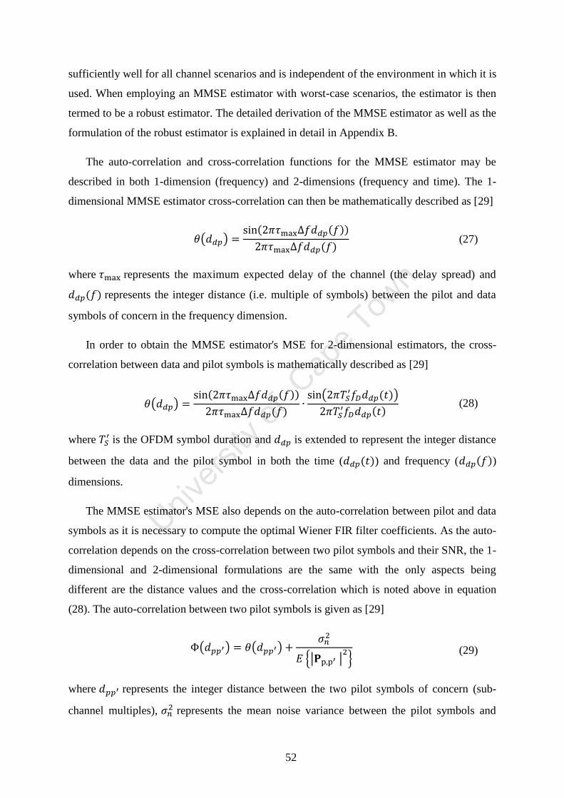
52

sufficiently well for all channel scenarios and is independent of the environment in which it is

used. When employing an MMSE estimator with worst-case scenarios, the estimator is then

termed to be a robust estimator. The detailed derivation of the MMSE estimator as well as the

formulation of the robust estimator is explained in detail in Appendix B.

The auto-correlation and cross-correlation functions for the MMSE estimator may be

described in both 1-dimension (frequency) and 2-dimensions (frequency and time). The 1-

dimensional MMSE estimator cross-correlation can then be mathematically described as [29]

where represents the maximum expected delay of the channel (the delay spread) and

represents the integer distance (i.e. multiple of symbols) between the pilot and data

symbols of concern in the frequency dimension.

In order to obtain the MMSE estimator's MSE for 2-dimensional estimators, the cross-

correlation between data and pilot symbols is mathematically described as [29]

where is the OFDM symbol duration and is extended to represent the integer distance

between the data and the pilot symbol in both the time ( ) and frequency ( )

dimensions.

The MMSE estimator's MSE also depends on the auto-correlation between pilot and data

symbols as it is necessary to compute the optimal Wiener FIR filter coefficients. As the auto-

correlation depends on the cross-correlation between two pilot symbols and their SNR, the 1-

dimensional and 2-dimensional formulations are the same with the only aspects being

different are the distance values and the cross-correlation which is noted above in equation

(28). The auto-correlation between two pilot symbols is given as [29]

where represents the integer distance between the two pilot symbols of concern (sub-

channel multiples), represents the mean noise variance between the pilot symbols and

( )

(27)

( )

(

)

(28)

( ) ( )

{| | } (29)

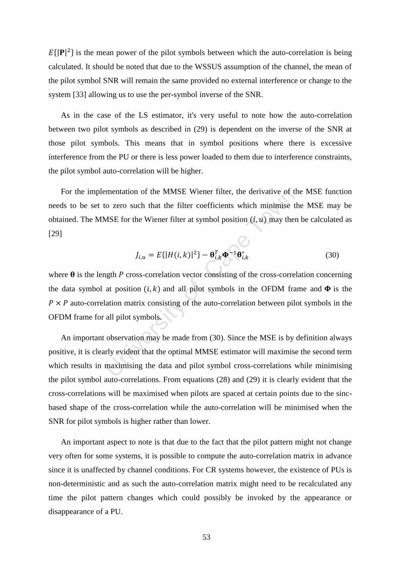
53

{| | } is the mean power of the pilot symbols between which the auto-correlation is being

calculated. It should be noted that due to the WSSUS assumption of the channel, the mean of

the pilot symbol SNR will remain the same provided no external interference or change to the

system [33] allowing us to use the per-symbol inverse of the SNR.

As in the case of the LS estimator, it's very useful to note how the auto-correlation

between two pilot symbols as described in (29) is dependent on the inverse of the SNR at

those pilot symbols. This means that in symbol positions where there is excessive

interference from the PU or there is less power loaded to them due to interference constraints,

the pilot symbol auto-correlation will be higher.

For the implementation of the MMSE Wiener filter, the derivative of the MSE function

needs to be set to zero such that the filter coefficients which minimise the MSE may be

obtained. The MMSE for the Wiener filter at symbol position may then be calculated as

[29]

where is the length cross-correlation vector consisting of the cross-correlation concerning

the data symbol at position and all pilot symbols in the OFDM frame and is the

auto-correlation matrix consisting of the auto-correlation between pilot symbols in the

OFDM frame for all pilot symbols.

An important observation may be made from (30). Since the MSE is by definition always

positive, it is clearly evident that the optimal MMSE estimator will maximise the second term

which results in maximising the data and pilot symbol cross-correlations while minimising

the pilot symbol auto-correlations. From equations (28) and (29) it is clearly evident that the

cross-correlations will be maximised when pilots are spaced at certain points due to the sinc-

based shape of the cross-correlation while the auto-correlation will be minimised when the

SNR for pilot symbols is higher rather than lower.

An important aspect to note is that due to the fact that the pilot pattern might not change

very often for some systems, it is possible to compute the auto-correlation matrix in advance

since it is unaffected by channel conditions. For CR systems however, the existence of PUs is

non-deterministic and as such the auto-correlation matrix might need to be recalculated any

time the pilot pattern changes which could possibly be invoked by the appearance or

disappearance of a PU.

{| | }

(30)

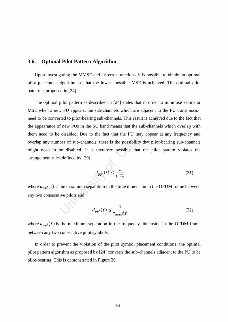
54

3.6. Optimal Pilot Pattern Algorithm

Upon investigating the MMSE and LS error functions, it is possible to obtain an optimal

pilot placement algorithm so that the lowest possible MSE is achieved. The optimal pilot

pattern is proposed in [24].

The optimal pilot pattern as described in [24] states that in order to minimise estimator

MSE when a new PU appears, the sub-channels which are adjacent to the PU transmission

need to be converted to pilot-bearing sub-channels. This result is achieved due to the fact that

the appearance of new PUs in the SU band means that the sub-channels which overlap with

them need to be disabled. Due to the fact that the PU may appear at any frequency and

overlap any number of sub-channels, there is the possibility that pilot-bearing sub-channels

might need to be disabled. It is therefore possible that the pilot pattern violates the

arrangement rules defined by [29]

where is the maximum separation in the time dimension in the OFDM frame between

any two consecutive pilots and

where is the maximum separation in the frequency dimension in the OFDM frame

between any two consecutive pilot symbols.

In order to prevent the violation of the pilot symbol placement conditions, the optimal

pilot pattern algorithm as proposed by [24] converts the sub-channels adjacent to the PU to be

pilot-bearing. This is demonstrated in Figure 20.

(31)

(32)

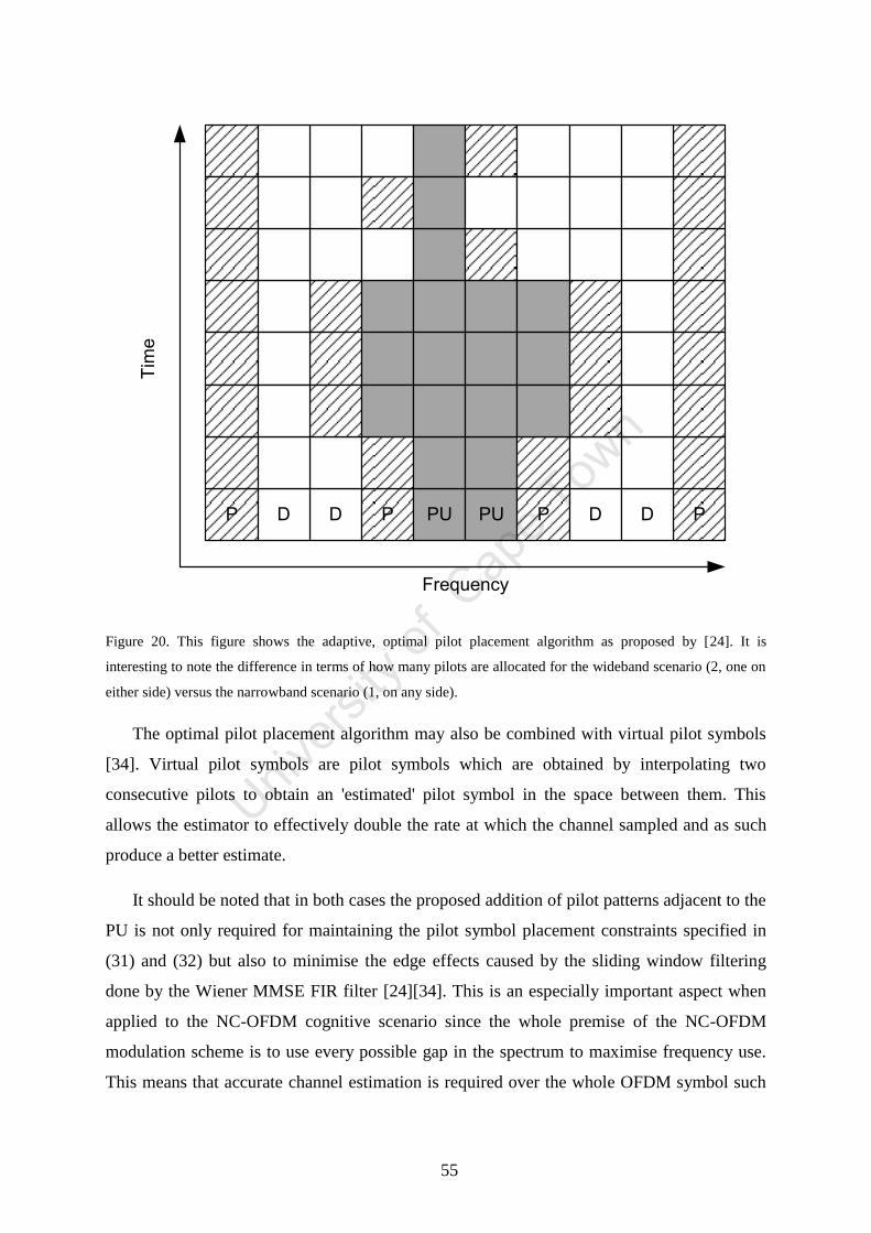
55

P D P PU PU P D PD D

Frequency

Tim

e

Figure 20. This figure shows the adaptive, optimal pilot placement algorithm as proposed by [24]. It is

interesting to note the difference in terms of how many pilots are allocated for the wideband scenario (2, one on

either side) versus the narrowband scenario (1, on any side).

The optimal pilot placement algorithm may also be combined with virtual pilot symbols

[34]. Virtual pilot symbols are pilot symbols which are obtained by interpolating two

consecutive pilots to obtain an 'estimated' pilot symbol in the space between them. This

allows the estimator to effectively double the rate at which the channel sampled and as such

produce a better estimate.

It should be noted that in both cases the proposed addition of pilot patterns adjacent to the

PU is not only required for maintaining the pilot symbol placement constraints specified in

(31) and (32) but also to minimise the edge effects caused by the sliding window filtering

done by the Wiener MMSE FIR filter [24][34]. This is an especially important aspect when

applied to the NC-OFDM cognitive scenario since the whole premise of the NC-OFDM

modulation scheme is to use every possible gap in the spectrum to maximise frequency use.

This means that accurate channel estimation is required over the whole OFDM symbol such

56

that all sub-channels may be used to conduct transmissions between the different devices

implemented as the SUs.

3.7. Contributions

The models presented in this chapter were essential to the development of the proposed

solution. As the solution needed to be modelled, the first contribution presented here is the

identification of the contradiction problem presented by the optimal pilot pattern and optimal

power loading algorithms for NC-OFDM cognitive radios.

This chapter specifically focuses on the mathematical models and characteristics used by

the optimal pilot pattern and power loading algorithms such that an optimal solution may be

derived for their contradicting nature. The models are then used further in Chapter 4 to

develop and derive new models whereby the identified problem of their contradiction is

solved using the new models.

57

4. Optimal Pilot Patterns Using Optimal Power Loading

The system model described in Section 3 may be used to formulate a constrained

multivariate optimisation problem. The problem however also needs to be constrained by

limits such as the maximum power available for transmission as well as the maximum

amount of interference which may be introduced to the PUs by the SU. The formulation and

description of the constrained multivariate problem is described in Section 4.1.

Once the problem is correctly formulated, an appropriate solution may be offered. This

process and the solution itself are described in Section 4.2. Section 4.2 also elaborates on the

different approaches to solving the optimisation problem when dealing with a 1-dimensional

and a 2-dimensional estimator. The approaches are compared and a generalised algorithm is

derived for both cases such that a simple, practical implementation may be easily obtained.

Sections 4.3 and 4.4 go on to describe the implementation of the generalised solution

algorithm in situations where the LS (Section 4.3) and the MMSE (Section 4.4) estimators are

utilised. Both sections describe the estimator-specific solution for both the 1-dimensional and

2-dimensional estimator implementation in terms of how the heuristic function differs in

application to the generalised solution algorithm.

Section 4.5 contains a description as well as analysis of the computational complexity of

the algorithm used to solve the constrained multivariate optimisation problem. The algorithm

computational complexity is analysed from both a computational time and memory

requirement aspects. The analysis is then further broken down for several sections of the

algorithms; implementation-stage optimisations are then proposed. Finally, a sub-optimal

algorithm is proposed as a variant of the generalised optimal algorithm while factoring in any

sub-optimal versions of the power loading algorithm.

4.1. Formulation as a Constrained Multivariate Optimisation Problem

The solution to the problem may be looked at from two points of view depending on the

degrees of freedom; these are whether to obtain an optimal power loading such that the

optimal pilot pattern is satisfied or to obtain an optimal pilot pattern such that the optimal

power loading is maintained.

58

In the former approach this translates to applying the optimal pilot pattern as specified in

Section 3.6 and then power loading the pilot symbols such that the lowest MSE is achieved.

This approach favours the estimator MSE instead of the overall transmission capacity and

does not take into consideration more stringent interference and transmission power limits.

The latter approach involves the application/calculation of the optimal power loading

algorithm as described in Section 3.3 such that the power loaded to each symbol in the

OFDM symbol of interest is calculated. The pilot patterns are then calculated depending on

the lowest MSE achievable when the pilot symbols are placed at all possible positions given

the power loading assigned to those positions. This approach favours the overall transmission

capacity as the optimal power loading algorithm is a solution to a constrained optimisation

function where the chief goal is to maximise transmission capacity [19]. Due to the inherent

interference constraints caused by the SU to the PU superseding the SU information rate [1],

this was the approach chosen as the objective function in order to achieve the optimal

solution to the constrained optimisation problem.

Since the primary function of a cognitive radio is to control its interference to licensed

users, followed by its secondary function of maximising its data rate, the approach followed

as described in the previous paragraph allows us to obtain the constrained, multivariate

optimisation problem. The mathematical description is

such that

where denotes the heuristic function associated with the estimator in use such that the error

is described as a function of power and pilot position.

From the equations listed above, the objective function in (33) may be seen to be the

minimisation of the estimator MSE as a function of the optimal power loading algorithm

∑ ∑ {|

| }

(33)

∑ ∑

(34)

(35)

| | (36)

| | (37)

59

applied to all symbols in the OFDM frame. The purpose of this is such that a candidate pilot

placement/pattern may be chosen and the constrained, multivariate objective function is used

to determine the overall MSE of the estimator in the given OFDM frame.

Due to the fact that all estimator MSE functions depend on the distance pilot

arrangement/pattern and hence the distance between the pilot symbols nearest to a PU and the

PU edge itself, the heuristic function is indeed shown to be a function of the pilot positions

p. When factoring this with the fact that there is a limit to the total power that may be loaded

to all symbols due to transmission power regulations as well as the placement of pilot

symbols dictated by the arrangement rules for sampling the channel in (31) and (32), the

optimisation problem is indeed a case of constrained, multivariate optimisation. The problem

is however also one of non-linear optimisation due to the presence of non-linear terms used to

describe the error of both the LS and MMSE estimators as well as the non-linear terms used

in the integrals modelling the out-of-band interference from both the PUs and SUs when

considering the optimal power loading algorithm.

Most non-linear, constrained optimisation problems may be solved through the utilisation

of the Karush-Kuhn-Tucker (KKT) conditions. The solution of a problem through the use of

the KKT conditions allows for an optimal, proven solution of the non-linear optimisation

problem [35]. The use of the KKT conditions is indeed the best approach to determining the

analytical solution to the optimisation problem, as mathematically stated in equations (33)-

(37), however it is hindered by a major property inherent in the estimator error functions,

which is the presence of transcendental functions in the estimator error functions.

Transcendental functions are ones which are unable to satisfy any polynomial equations

whose coefficients are polynomials themselves [36]. These functions are therefore not able to

be represented as a finite series of algebraic operations. Examples of transcendental functions

include the trigonometric functions, the exponential function as well as the logarithm.

Due to the presence of trigonometric, specifically sinusoidal (and hence transcendental)

terms in the pulse-shaping function used to model both the PU and the SU transmissions, the

optimal power loading algorithm, specifically the interference components, will contain

periodic functions. This presents a unique challenge when attempting to find the global

minimum, and hence the optimal solution, for the multivariate optimisation problem. In the

case of how the optimal power loading solution was obtained in [19] there is indeed an

analytical solution able to find the global minimum and hence the optimal solution while

60

using the same sinusoidal-based pulse-shaping functions to model the interference. There is

however one major difference and that is the fact that symbol position/placement is not a

direct constraint requirement in the optimisation function. This means that the solution could,

and indeed does, have a unique global minimum due to the periodic nature and hence

multiple global minima not being present as a prerequisite. The detailed mathematical

derivation of this may be found in Appendix A. Upon further investigation, it was therefore

decided that the problem would prove to be infeasible to solve analytically through the use of

the KKT conditions due to the presence of transcendental functions in the constraint

conditions [37]. Even though the existence of transcendental functions in the constraint

conditions meant that an analytical solution would not be feasible, several attempts were still

made at obtaining an analytical solution, including the use of Wolfram's Mathematica

package for computer-based symbolic equation solver. The Minimize function was used in

Mathematica which specifically attempts to find the symbolic, global minimum of a set of

provided functions and constraints but none could be found by the software package. It was

therefore decided that the best solution was through the use of numerical methods and

computation because an analytical approach was deemed highly infeasible due to the required

constraints providing an ambiguity in finding the global minimum.

The optimisation problem specified by equations (33) – (37) is the generalised

optimisation function which allows the whole pilot pattern to be determined. This algorithm

allows us to find the optimal solution for the pilot placement for all pilot symbols in the

OFDM frame while maintaining the necessary power loading so as to constrain interference.

However, due to the possibly limited presence of PUs in the SU band, the interference to and

from the PUs would not necessarily pose any significant effect on all of the SU's sub-

channels, rather only the ones relatively close to the PUs. This means that the algorithm need

not be calculated over the whole OFDM symbol but instead a classic, static pilot pattern may

be maintained for the SU. It is therefore only necessary to perform the computation in the

regions between the PU transmission edges and the nearest unaffected, static pilot symbol.

This is in accordance with the optimal pilot pattern as proposed in [24][34] such that the

focus is on mitigating the effects of the lost channel samples (pilots) where sub-channels

needed to be disabled in order to affect overlapping with a PU.

The calculation constraint on the algorithm allows the optimality to be maintained due to

the insignificant effects by the PU on sub-channels farther away as well as significantly

decreasing the computational time and effort required to find the optimal pilot placement.

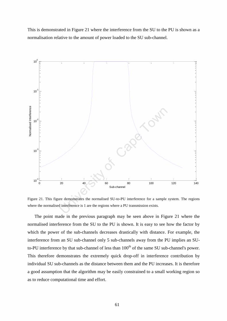
61

This is demonstrated in Figure 21 where the interference from the SU to the PU is shown as a

normalisation relative to the amount of power loaded to the SU sub-channel.

Figure 21. This figure demonstrates the normalised SU-to-PU interference for a sample system. The regions

where the normalised interference is 1 are the regions where a PU transmission exists.

The point made in the previous paragraph may be seen above in Figure 21 where the

normalised interference from the SU to the PU is shown. It is easy to see how the factor by

which the power of the sub-channels decreases drastically with distance. For example, the

interference from an SU sub-channel only 5 sub-channels away from the PU implies an SU-

to-PU interference by that sub-channel of less than 100th

of the same SU sub-channel's power.

This therefore demonstrates the extremely quick drop-off in interference contribution by

individual SU sub-channels as the distance between them and the PU increases. It is therefore

a good assumption that the algorithm may be easily constrained to a small working region so

as to reduce computational time and effort.

0 20 40 60 80 100 120 14010

-4

10-3

10-2

10-1

100

Sub-channel

Norm

alis

ed I

nte

rfere

nce

62

An important aspect which may be observed is that the minimisation problem as

described in (33) – (37) may be implemented as a different solution for 1-dimensional and 2-

dimensional estimators. For 1-dimensional estimators, i.e. ones which focus only on the

frequency dimension and have no memory in terms of the time dimension, the optimisation

problem may be implemented as a memory-less algorithm. This means that for every OFDM

symbol, the pilot placement for the sub-channels of interest could be determined such that the

optimal pilot symbol is found. For the next OFDM symbol however, the memory-less

algorithm would not consider the pilot placement in the previous OFDM symbol and as such

would only consider the current estimator MSE and power loading for the current OFDM

symbol. This approach is the most trivial but there is an alternative approach where the pilot

placement for previous OFDM symbols is kept in memory an utilised for the current OFDM

symbol. The memory based approach for the optimal solution to the optimisation problem

would require the algorithm solving the optimisation problem to consider the pilot placement

in the previous OFDM symbols such that the estimator MSE is minimised in the sense of the

OFDM frame rather than just the OFDM symbol in the memory-less approach. It would

therefore make sense to implement a 1-dimensional solution for 1-dimensional estimators and

correspondingly a 2-dimensional solution for 2-dimensional estimators.

4.2. Generalised Solution and Algorithm

In order to develop a solution to the constrained, non-linear multivariate optimisation

problem, a generalised algorithm needed to be devised such that the optimal pilot position

could be calculated. The optimal solution algorithm could then be implemented in the

cognitive radio devices such that the optimal pilot pattern could be computed for the current

situation in terms of the transmissions of PUs in the SUs' band. The algorithm would also

need to be executed any time the state of the PU transmissions in the SU band change. In

other words in situations such as when a PU appears or disappears, or when the transmission

power of a PU changes, or when the bandwidth of any PU transmission changes, the

algorithm will need to compute the new, optimal pilot pattern to utilise for future

transmissions.

The generalised, optimal solution algorithm would need to be independent of the

estimator type in so far as that an error, or more appropriately heuristic, function could be

substituted into the algorithm where necessary. This heuristic function would be used as a

63

measure of the desired estimator's (i.e., LS or MMSE) fitness and would allow the algorithm

to maintain its optimality. The heuristic function being a measure of the fitness of an

estimator, it would therefore be trivial to have it represent the MSE of the estimator of

concern due to its suitability for comparing an estimate's accuracy.

The use of a heuristic function to describe the fitness of a proposed pilot pattern given the

power-loading and channel state information was deemed as a vital approach to solving the

research problem in a structural and methodical way. By describing the fitness of the

proposed pilot patterns as one function, this allowed the solution-searching algorithm to be

generalised and described as one, unchanging algorithm for different estimator types. In

practical implementations, this means that the same algorithm may be used for several

different types of estimators whereby the only change necessary would just be the

formula/function used to decide on the fitness of the proposed pilot-pattern.

A side-benefit to the use of heuristic functions is also that they provide a fitness

measurement which does not have to be used with the proposed, generalised solution

algorithm but with any search algorithm decided to be implemented due to the heuristic

functions' independence and modularity of the search algorithm.

The optimal solutions for both the 1-dimensional and 2-dimensional estimators are

proposed in this section. Section 4.2.1 proposes a solution for the optimisation problem

described in (33)-(37) when a 1-dimensional estimator is utilised. This demonstrates how the

solution would be used to find the optimal pilot placement for the current OFDM symbol

without considering any past or future OFDM symbols. Section 4.2.2 then demonstrates how

the 1-dimensional estimator solution can be generalised and therefore used for 2-dimensional

estimators. This provides us with an algorithm allowing the optimal pilot placement to be

found when considering the current and previous OFDM symbols. This means that the

algorithm may then be extended to any number of OFDM symbols and consequently

providing us with the general solution to the constrained, multivariate optimisation problem.

4.2.1. 1-dimensional implementation

The most trivial and simple implementation of the solution to the proposed optimisation

problem of finding the optimal pilot placement for the adaptive pilot symbols given the

optimal power loading is one where each OFDM symbol is considered independently of one

64

another, meaning that the solution is considered and run one OFDM symbol at a time. The

optimal, 1-dimensional estimator solution would then be mathematically written as

The solution would then simply compute the objective function specified in (38) and

place the adaptive pilot symbols at the candidate pilot positions with the lowest objective

function value.

The 1-dimensional solution could therefore be implemented as an outer loop for all the

candidate pilot positions which iterates through them while the inner loop then simply iterates

through all the symbols in the OFDM symbol to obtain what the overall estimator MSE of the

OFDM symbol would be if the adaptive pilot were to be placed in the candidate position

currently being investigated.

4.2.2. 2-dimensional implementation

To be able to solve the optimisation problem stated in (33)-(37) for the 2-dimensional

estimator scenario, a generalised optimal algorithm needed to be developed. The algorithm

itself is stated as Algorithm 1 and is assumed that the optimal power loading algorithm has

already been executed for the current OFDM symbol and that the power loaded to each

symbol is known so that the heuristic function may be computed.

∑ {|

| }

(38)

65

Algorithm 1. This algorithm implements the proposed optimal solution.

k denotes current OFDM symbol (time)

Place pilots in traditional, fixed/static pattern

for each candidate pilot symbol position p' do

set accumulator = 0

for x = k down to 1 do

for y = 1 to NFFT do

Compute error heuristic between candidate position p' and (x , y)

accumulator = accumulator +

end for

end for

end for

Place new, adaptive pilots at two candidate positions with lowest accumulator value

The demonstrated algorithm is computed in 3 major, nested loops. The outer loop is used

to cycle through all the candidate positions for the pilot symbol. The outer loop of the

algorithm is used to iterate through the possible pilot symbol positions which could be used

for the placement of the adaptive pilot symbols. This would be the region between a PU's

band edge and the nearest, enabled static pilot symbol as stipulated by [24]. The two loops

nested in the outer loop are then used to calculate the error/heuristic function for the

candidate pilot symbol (i.e., if the pilot symbol were to be placed at the candidate position)

for every symbol in the current and previous OFDM symbols. This is done due to the fact that

the pilot symbols are placed at the optimal position in the current OFDM symbol since an

OFDM transmission is conducted one symbol at a time as well as the fact that any future

OFDM symbols might have different characteristics in terms of PU transmissions. As we

assume that we do not have any knowledge of what the future OFDM symbols in the OFDM

frame will be or that we cannot predict when and where PUs will appear in the future, we

may only test against pilot positioning in the current and previous OFDM symbols. This is

also done so as to exploit the correlation present in slowly-varying channels where the CFR

for each OFDM symbol will change slowly relative to each OFDM symbol.

It is also necessary when allocating the optimal pilot symbol positions that the validity is

checked according to equations (31) and (32) such that the chosen pilots do not invalidate any

66

channel sampling rules. If they are found to, the cognitive radio may then simply move on to

the candidate position which had the next lowest accumulation/error heuristic which is also

valid. Should there be no position where the candidate pilot symbol will maintain the

sampling rules, it would mean that the search area (i.e. candidate positions) is too small.

It is necessary to note that the algorithm described as Algorithm 1 is the generalisation of

the 1-dimensional estimator solution to the 2-dimensional scenario. If the 2-dimensional

scenario is computed on a per OFDM symbol basis with no memory component, Algorithm 1

will become the optimal solution for the 1-dimensional channel estimator.

4.3. LS Estimator Heuristic

In order to utilise the optimal, general algorithm for LS estimator-specific situations, a

heuristic function needed to be developed for the LS estimator such that the estimator MSE

could be quantified as a function of pilot placement and power loading. The function

heuristic function developed needed to quantify the estimator fitness as a function of the

current, candidate pilot pattern as well as the power loaded to all symbols in the OFDM

symbol (for 1-dimensional estimators) or the OFDM frame (for 2-dimensional estimators).

When deriving the heuristic function for the LS estimator, the different estimator types

need to be considered as well. The 1-dimensional estimator would trivially provide us with a

simpler heuristic function as a smaller search area is utilised, that is the current OFDM

symbol is the search area instead of the current and all previous OFDM symbols in the

OFDM frame for 2-dimensional estimators.

Due to the possible use of several types of interpolators, the heuristic for the LS estimator

will vary with each different type of interpolator used for channel estimation. The most basic

type of interpolator is the linear interpolator and as such was deemed necessary for

demonstration as it forms the basis for all higher-order interpolation as described in

Section 3.4. The 1-dimensional heuristic function for the LS estimator with a linear

interpolator is therefore

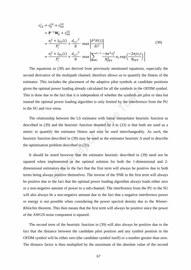
67

The equations in (39) are derived from previously mentioned equations, especially the

second derivative of the multipath channel; therefore allows us to quantify the fitness of the

estimator. This includes the placement of the adaptive pilot symbols at candidate positions

given the optimal power loading already calculated for all the symbols in the OFDM symbol.

This is done due to the fact that it is independent of whether the symbols are pilot or data but

instead the optimal power loading algorithm is only limited by the interference from the PU

to the SU and vice versa.

The relationship between the LS estimator with linear interpolator heuristic function as

described in (39) and the heuristic function denoted by in (33) is that both are used as a

metric to quantify the estimator fitness and may be used interchangeably. As such, the

heuristic function described in (39) may be used as the estimator heuristic used to describe

the optimisation problem described in (33).

It should be noted however that the estimator heuristic described in (39) need not be

squared when implemented as the optimal solution for both the 1-dimensional and 2-

dimensional estimators due to the fact that the first term will always be positive due to both

terms being always positive themselves. The inverse of the SNR in the first term will always

be positive due to the fact that the optimal power loading algorithm always loads either zero

or a non-negative amount of power to a sub-channel. The interference from the PU to the SU

will also always be a non-negative amount due to the fact that a negative interference power

or energy is not possible when considering the power spectral density due to the Wiener-

Khinchin theorem. This then means that the first term will always be positive since the power

of the AWGN noise component is squared.

The second term of the heuristic function in (39) will also always be positive due to the

fact that the distance between the candidate pilot position and any symbol position in the

OFDM symbol will be either zero (the candidate symbol itself) or a number greater than zero.

The distance factor is then multiplied by the maximum of the absolute value of the second

|

|

|∑

(

)

|

(39)

68

derivative of the CFR between the candidate symbol and the current symbol being iterated.

As this is an absolute value, it will also be always positive by definition and as such meaning

that the second term of the heuristic function will be always positive itself. This coupled with

the fact that the first term is always positive and the addition between the two terms means

that the error heuristic function will always be positive. It is therefore not necessary to square

the heuristic function specified in (39) as we are only seeking to compare positions according

to which one has the lowest error heuristic rather than the actual MSE. This is because the

heuristic function squared and then a mean of it at all positions providing us with the MSE

means that the estimator MSE is proportional to the heuristic function. As such, a lower

heuristic function will translate to a lower estimator MSE. We therefore may simply use the

heuristic function provided in (39) to quantify the best candidate pilot positions such that the

optimal adaptive pilot pattern may be obtained which minimises the LS estimator MSE when

utilising a linear interpolator.

In order to obtain an error heuristic function for scenarios where a 2-dimensional LS

estimator is required with the use of a linear interpolator, the 1-dimensional heuristic function

for the same estimator could then be extended to a 2-dimensional estimator provided that the

correct estimator MSE could be described. The 2-dimensional heuristic function may

therefore be described mathematically as

The 2-dimensional heuristic function described above in (40) is simply the conversion of

the 1-dimensional heuristic function to include distances evaluated in the two dimensions.

The major change is through the inclusion of the Euclidian distance parameter in determining

the maximum value of the second-order derivative of the channel frequency response. This is

accomplished through the use of the standard Euclidian distance obtainable from the

Pythagorean Theorem due to the rectangular nature of the time-frequency grid.

|∑

(

⌊√ ⌋

)

|

(40)

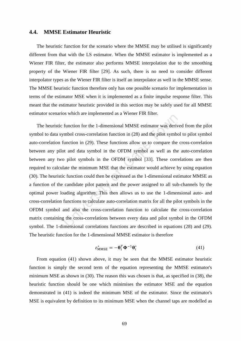
69

4.4. MMSE Estimator Heuristic

The heuristic function for the scenario where the MMSE may be utilised is significantly

different from that with the LS estimator. When the MMSE estimator is implemented as a

Wiener FIR filter, the estimator also performs MMSE interpolation due to the smoothing

property of the Wiener FIR filter [29]. As such, there is no need to consider different

interpolator types as the Wiener FIR filter is itself an interpolator as well in the MMSE sense.

The MMSE heuristic function therefore only has one possible scenario for implementation in

terms of the estimator MSE when it is implemented as a finite impulse response filter. This

meant that the estimator heuristic provided in this section may be safely used for all MMSE

estimator scenarios which are implemented as a Wiener FIR filter.

The heuristic function for the 1-dimensional MMSE estimator was derived from the pilot

symbol to data symbol cross-correlation function in (28) and the pilot symbol to pilot symbol

auto-correlation function in (29). These functions allow us to compare the cross-correlation

between any pilot and data symbol in the OFDM symbol as well as the auto-correlation

between any two pilot symbols in the OFDM symbol [33]. These correlations are then

required to calculate the minimum MSE that the estimator would achieve by using equation

(30). The heuristic function could then be expressed as the 1-dimensional estimator MMSE as

a function of the candidate pilot pattern and the power assigned to all sub-channels by the

optimal power loading algorithm. This then allows us to use the 1-dimensional auto- and

cross-correlation functions to calculate auto-correlation matrix for all the pilot symbols in the

OFDM symbol and also the cross-correlation function to calculate the cross-correlation

matrix containing the cross-correlations between every data and pilot symbol in the OFDM

symbol. The 1-dimensional correlations functions are described in equations (28) and (29).

The heuristic function for the 1-dimensional MMSE estimator is therefore

From equation (41) shown above, it may be seen that the MMSE estimator heuristic

function is simply the second term of the equation representing the MMSE estimator's

minimum MSE as shown in (30). The reason this was chosen is that, as specified in (38), the

heuristic function should be one which minimises the estimator MSE and the equation

demonstrated in (41) is indeed the minimum MSE of the estimator. Since the estimator's

MSE is equivalent by definition to its minimum MSE when the channel taps are modelled as

(41)

70

i.i.d. Gaussian processes [26], the function was chosen to be the second term of its MMSE

such that when it is maximised it will essentially minimise the MSE. This holds true due to

the fact that the estimator MSE will always be a positive value by definition and applies in

this case due to practical concerns, the Wiener FIR filter is designed such that the filter

coefficients are real. This reduces computational complexity and furthermore halves the

computational effort when the filter is implemented as 2x1-dimensional cascaded filter [29].

The use of real-only coefficients is a very practical assumption also due to the fact that the

channel correlation matrix is always a Hermitian matrix which is always positive-

semidefinite. These properties mean that the diagonal of the channel correlation matrix has a

strictly real diagonal (Hermitian property) which will always be positive (positive-

semidefinite) due to the Wiener-Khinchin theorem applying to the channel's PSD and its

corresponding gains.

The estimator MMSE mentioned above in equation (30) for the 1-dimensional scenario

may then be, through the process of simple substitution, represented as an equation consisting

of trigonometric functions. This is because the channel autocorrelation function and therefore

Doppler spectrum have to be assumed to be the worst-case due to not knowing the exact

values. This is done by design and is in fact the reason and purpose behind the development

and use of what's known as robust estimators. The substitution of the sinc functions into the

matrix multiplication is also in part due to the fact that in practical implementations, the

Wiener FIR filter coefficients are chosen to be real-valued so as to reduce their computational

complexity [29] but also due to the fact that the auto-correlation and cross-correlation

matrices may be computed iteratively. As such, the error function value may be represented

as a function of the trigonometric, robust cross-correlation and auto-correlation functions as

( )

{| | }

{| | }

(42)

71

In order to have a heuristic function for the optimal algorithm when a 2-dimensional

estimator is utilised, the 1-dimensional heuristic function needed to be extended. Due to the

nature of the 2-dimensional solution, the cross-correlation function between the pilot and data

symbols needed to be used instead of the 1-dimensional as per the 1-dimensional estimator

solution from which it is derived from. The 2-dimensional heuristic function for the MMSE

estimator may then be described as [29]

It's easily noted that the solution described in the equation above is simply the extension

of the 1-dimensional heuristic function with the exception that the cross-correlation vector

becomes a cross-correlation matrix storing the cross-correlations between the symbol at

position (i,k) and all data symbols in the OFDM frame. There is however the added element

of the two-dimensional correlation calculations demonstrated below in equation (44). This

obviously adds computational complexity and calculation time requirement to the heuristic

function.

4.5. Algorithm Complexity and Sub-Optimal Solutions

The proposed optimal solution algorithm in the previous sections also requires great

consideration of its implementation efficiency and general practicality such that the algorithm

may be efficiently implemented on current SDR hardware rather than just remain a

theoretical concept. It was therefore deemed necessary to analyse the generalised optimal

solution algorithm in terms of its memory space and computational time so that it was

deemed whether a direct implementation would be feasible or whether a sub-optimal

implementation was needed such that a more practical implementation could be achieved.

(43)

( )

( )

{| | }

( )

( )

{| | }

(44)

72

4.5.1. Algorithm complexity

The algorithm complexity may be analysed in two major aspects, namely the

computational time and the memory space requirement. The algorithm may be analysed

through the use of Bachmann-Landau notation, specifically the use of the upper-bound

limiting notation known as big-O notation [38] such that the limiting behaviour may be

described for the generalised optimal solution algorithm in both the calculation time and

memory space aspects. This therefore represents the worst-case scenario for the

computational time and memory space of the algorithm for asymptotically large input sizes

denoted by n.

Upon analysing the general solution algorithm, it may be easily seen that the algorithm's

computational time may be written in big-O notation as . This means that as the input

data to the algorithm increases to infinity, the calculation time required to compute the

solution provided by the general algorithm will be bounded above by the cube of the size of

the input data set. This is mainly attributable to the fact that most of the computation time

done by the generalised algorithm is spent in iterating through the three nested for loops. This

computational time is also commonly known as polynomial time where the big-O notation is

for all c > 1 and specifically cubic time for when c = 3 as is the situation for the

generalised solution algorithm [38].

The memory space requirements of the generalised solution algorithm may also be

represented by the big-O notation to denote the asymptotic upper bound of the memory space

requirement needed for computation of the solution through the generalised algorithm given

an input of size n. The memory space requirement could therefore be represented in big-O

notation as , this is due to the fact that the generalised solution algorithm only requires a

constant amount of extra memory depending on the number of candidate pilot positions. The

memory space requirement will therefore be dominated by the linear memory space required

for storing the OFDM symbols rather than the constant memory space needed to store the

accumulator used for comparison of candidate pilot positions.

It was therefore obvious that the generalised solution algorithm has a good memory space

upper bound, , but also has a high computational time requirement, , for any input

set n. This meant that a solution with a lower computational complexity needed to be found

since the high computational complexity could prove to significantly slow down the signal

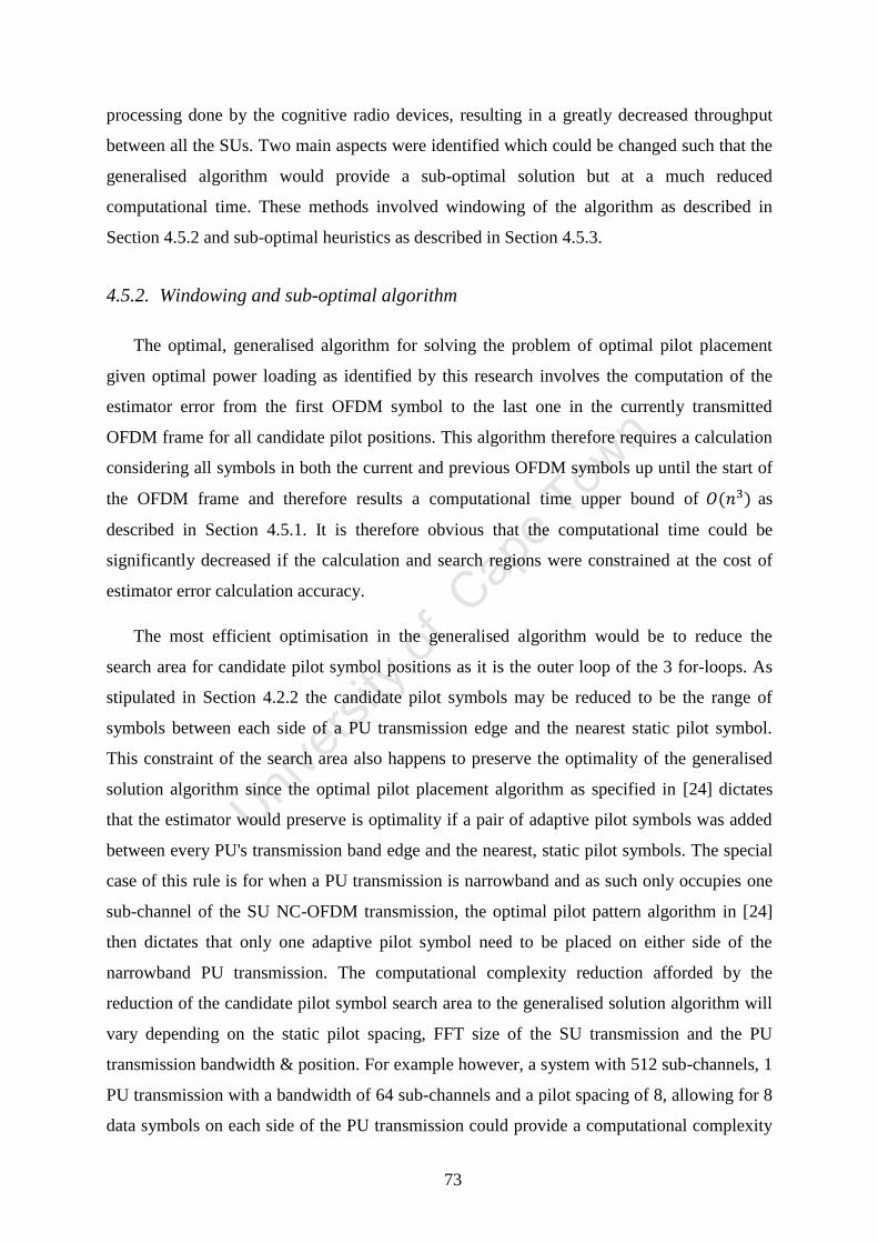
73

processing done by the cognitive radio devices, resulting in a greatly decreased throughput

between all the SUs. Two main aspects were identified which could be changed such that the

generalised algorithm would provide a sub-optimal solution but at a much reduced

computational time. These methods involved windowing of the algorithm as described in

Section 4.5.2 and sub-optimal heuristics as described in Section 4.5.3.

4.5.2. Windowing and sub-optimal algorithm

The optimal, generalised algorithm for solving the problem of optimal pilot placement

given optimal power loading as identified by this research involves the computation of the

estimator error from the first OFDM symbol to the last one in the currently transmitted

OFDM frame for all candidate pilot positions. This algorithm therefore requires a calculation

considering all symbols in both the current and previous OFDM symbols up until the start of

the OFDM frame and therefore results a computational time upper bound of as

described in Section 4.5.1. It is therefore obvious that the computational time could be

significantly decreased if the calculation and search regions were constrained at the cost of

estimator error calculation accuracy.

The most efficient optimisation in the generalised algorithm would be to reduce the

search area for candidate pilot symbol positions as it is the outer loop of the 3 for-loops. As

stipulated in Section 4.2.2 the candidate pilot symbols may be reduced to be the range of

symbols between each side of a PU transmission edge and the nearest static pilot symbol.

This constraint of the search area also happens to preserve the optimality of the generalised

solution algorithm since the optimal pilot placement algorithm as specified in [24] dictates

that the estimator would preserve is optimality if a pair of adaptive pilot symbols was added

between every PU's transmission band edge and the nearest, static pilot symbols. The special

case of this rule is for when a PU transmission is narrowband and as such only occupies one

sub-channel of the SU NC-OFDM transmission, the optimal pilot pattern algorithm in [24]

then dictates that only one adaptive pilot symbol need to be placed on either side of the

narrowband PU transmission. The computational complexity reduction afforded by the

reduction of the candidate pilot symbol search area to the generalised solution algorithm will

vary depending on the static pilot spacing, FFT size of the SU transmission and the PU

transmission bandwidth & position. For example however, a system with 512 sub-channels, 1

PU transmission with a bandwidth of 64 sub-channels and a pilot spacing of 8, allowing for 8

data symbols on each side of the PU transmission could provide a computational complexity

74

decrease by a factor of 28 or would reduce the number of loop iterations by 283 = 21952. This

is due to the fact that only 16 candidate pilot symbol positions need to be considered (8 on

each side of the PU transmission) instead of all 448 (7/8 x 512) data symbols.

Another solution reducing the computational time of the generalised algorithm is to

constrain the search area of the estimator error calculation done for all candidate pilot symbol

positions. This involves constraining the two inner loops of the generalised algorithm such

that pilot symbols within a certain area around the candidate symbol are considered. This is

known as windowing and is commonly employed during channel estimation as a trade-off

between computational complexity and estimation accuracy [29]. The same technique could

therefore be used to provide the same computational complexity and positioning accuracy to

the generalised algorithm proposed as the solution in this thesis. This would be especially

true if windowing is already employed for the implementation of the channel estimator as the

solution algorithm (Algorithm 1) does not need to consider symbols outside the estimator's

window such that the estimation accuracy may be optimised for the windowed estimator

rather than the optimal (no window) estimator which is not employed.

75

p

p

p

p

p

p

p

p

p

p

p

p

p

p

p

Frequency

Tim

e

Figure 22. This figure demonstrates the different iteration areas for calculating the heuristic function values for

candidate pilot symbol positions denoted by 'p'. The dotted rectangle represents the non-windowed calculation

region while the dashed rectangle indicates the windowed/constrained calculation region.

The premise of applying a window constraint to the generalised solution algorithm is

demonstrated in Figure 22 where the candidate pilot positions for each OFDM symbol are

indicated by the letter 'p'. The iteration region of the generalised algorithm is shown by the

dots, demonstrating how the algorithm iterates through the whole of the current and past

OFDM symbols to calculate the error heuristic functions for each each candidate position.

The application of a constrained/windowed iteration region is then shown by the dashed

rectangle for the candidate position indicated by the dot in the upper right corner. This shows

how the iteration is constrained to be a maximum of 3 symbols in either the time or frequency

dimension. The hatched blocks in Figure 22 represent pilot symbols placed according to the

static pilot pattern and the blocks with a darker shade represent the disabled symbols which

are occupied by a PU.

76

4.5.3. Sub-optimal heuristics

The sub-optimal generalised solution algorithm as described in the section above may

have its computational complexity further reduced by analysing the most computationally

intense functions inside it. These functions are namely the power loading algorithm and the

error heuristic functions.

The optimal power loading algorithm as derived in [19] also has sub-optimal variants

described in the same source. The sub-optimal solutions in [19] can be summarised as

exploiting two different facts about the power loading requirements. The first sub-optimal

scheme proposed takes advantage of the fact that the power is loaded in discrete steps per

sub-channel rather than as a continuous function since every sub-channel has a uniform

amount of power transmitted in it.

The second algorithm proposed by [19] as sub-optimal power loading simply exploits the

fact that PU-to-SU and SU-to-PU interference both increase as the distance between a PU and

a SU decreases and inversely both decrease as the distance between a PU and an SU

decreases. The sub-optimal algorithm then proposes that the first term of the optimal power

loading equation in (20) is dropped such that the optimisation constant and the only

interference indicator concerned is the derivative of the SU-to-PU interference, . The sub-

optimal power loading algorithm was therefore described as

This means that the sub-optimal power loading algorithm does not have to calculate the

PU-to-SU interference but even more importantly it means that the optimisation constant

does not need to be searched for. This then reduces the algorithm complexity from

to since a binary search need not be performed to find but rather just a

simple computation of readily available parameters.

It is very important to note that the generalised solution algorithm as proposed in

Algorithm 1 is independent of what type of heuristic function or power loading algorithm is

used as long as the power loading algorithm concerns the interference caused between the PU

and the SU and so long as the error heuristic function provides the capability to perform a

relative comparison between channel estimator accuracies for different candidate pilot

symbol positions. This means that the generalised algorithm is therefore versatile enough so

∑

(45)

77

that it may be used successfully for both optimal and sub-optimal power loading and error

heuristic functions with no modification to the actual algorithm itself.

The heuristic functions could have their computational complexity further reduced by

looking at them from a different perspective. The heuristic functions in the solution to the

problem stated by this research serve the purpose of allowing the solution algorithm to

compare one candidate pilot position against other candidate pilot positions. This is done

through the calculation of the overall estimator MSE for each candidate pilot position.

However, realising the fact that we only need to compare candidate pilot positions against

each other rather than a certain fixed benchmark, there exists the possibility of utilising

simplified heuristic functions which are much easier to compute and do not give a good

approximation of the MSE but rather a proportional one. It is therefore possible to use these

simplified heuristic functions purely for comparison against one another for different

candidate pilot positions as long as they are monotonically increasing when compared to their

respective MSE heuristic functions.

4.5.4. Heuristic function approximations

The previously mentioned methods for reducing the computational complexity of the

solution algorithm all focus on using the exactly derived heuristics functions for the different

application scenarios. There is however one very impacting way in which the computational

complexity of the solution algorithm could be changed and that is through the use of

approximated heuristic functions. Since the heuristic functions mainly consist of either

exponentials or trigonometric functions, the computation of these functions would itself be a

complex feat that's ever present in modern computation. In order to reduce the computation

however, these functions could be approximated to simpler functions which would be much

faster to execute. To some extent, this would be necessary with the optimal functions in any

case due to the practice of using look-up tables to compute approximate trigonometric

function values in embedded and low-power devices.

The main point to note when simplifying the LS and MMSE estimator heuristics is that

the solution algorithm is based purely on determining the candidate pilot position with the

best (lowest) estimator heuristic. This means that the actual MSEs of the candidate pilot

symbol positions are not relevant but only how they compare relative to other candidate pilot

symbol positions. The heuristics functions therefore only have to be comparative rather than

78

absolute and as such all the simplification of the heuristic functions has to achieve is an

accurate representation of the comparative difference between different candidate pilot

symbol positions.

The use of approximations to the heuristic functions could therefore centre on the use of

look-up tables for trigonometric functions, in this case the sinusoid function due to its

prevalence in the heuristic and power loading functions, especially for the MMSE estimator.

Since the error of the heuristic function may be relatively large due to the requirement for

only a relative comparison between different candidate pilot position sub-channels, the

sinusoids could be trivially enumerated and stored in a look-up table not requiring high

resolution due to the fact that inherent tolerance for small errors afforded by the discretisation

of the time-frequency grid as well as the nature of the problem only requiring a relative

comparison between different candidate pilot symbol positions rather than exact values.

4.5.5. Computational Complexity Implications

Given the computational complexity of the proposed optimal solution algorithm and sub-

optimal algorithms, their impact on run-time and accuracy is an important trade-off to be

considered for applications where computational time or space is severely limited.

Due to the exhaustive nature of the optimal solution algorithm, the algorithm would be

classified as an O(n3) algorithm for large n. This means that for applications where

computational power is plentiful, for example fixed base-stations, the computational time

should not be of much concern. On the other hand, for situations where computational time

and power is severely restricted, for example mobile user devices/terminals, the

computational complexity of the algorithm is severely prohibitive and could take up a

significant chunk of processing time.

It is logical that the sub-optimal algorithm then be used for situations where processing

power and computational time are at a premium. The sub-optimal algorithm affords much

reduced complexity by replacing sinusoidal computations with direct look-up tables,

windowing the search area and possibly using sub-optimal power loading for really extreme

cases. Due to the impact of windowing, the search time would by a factor equivalent to the

ratio of the window to the frame size combined with the conversion of sinusoidal calculations

79

to constant time due to the look-up table. This will however cause a reduction in accuracy

which is demonstrated in the next chapter.

4.6. Comparison to Similar Solutions

The contributions outlined in this chapter provide the optimal and sub-optimal solutions

to the identified problem. There has also been work done on finding the optimal pilot pattern

in NC-OFDM cognitive radios while also considering power loading for pilot symbols. This

is demonstrated in work such as [51] and [52].

The most critical point to note with regards to solutions proposed in related work

however is that they only focus on power loading to pilot symbols in a blind manner without

considering interference to and from primary users. This means that the proposed solutions

do not consider whether the interference threshold from the SU to the PU is violated due to

the proximity of pilot symbols as well as the reduction in channel sampling caused by extra

noise on the pilot symbols due to nearby SUs.

This approach is however effective (and indeed optimal) when there are no primary users

relatively close to the secondary users or when the SU sub-channels near to the PU are

disabled so as to altogether avoid the effects of out-of-band interference to and from the PU.

This does however mean that the throughput is reduced since there are now empty frequency

bins in the time-frequency grid.

The approaches proposed in [51] and [52] therefore breaks down when an optimal and

complete utilisation of the frequency spectrum between PUs is required due to the

aforementioned reasons. As such, the demonstrated solution algorithms solve the complete

scenario so that PU-SU interference is considered (as well as the power loading implications

it would have) when an optimal pilot pattern is calculated.

80

5. Simulation Details and Results

This section contains details describing the simulations performed to evaluate the validity

and performance of the proposed solutions to the identified problem of optimal pilot

placement given optimal power loading for NC-OFDM cognitive radios. The section is

divided into two sections describing simulation parameters and showing simulation results.

Section 5.1 describes the simulation parameters used when simulating the proposed

solutions in this research thesis. The section shows various different aspects and approaches

used to simulate the several combinations of solutions possible, namely 1-dimensional and 2-

dimensional as well as for all the different types of estimators, as proposed in this document.

Section 5.2 then demonstrates in detail the simulation results for various different

parameters deemed important to the performance and validity evaluation of the proposed

solutions. The section also provides an overview of the performance of the generalised

solution algorithm as well as a comparison to the proposed sub-optimal solutions such that

the implementation factors and concerns like the computational time and memory space

requirements may be evaluated so that the performance/MSE trade-off may be better gauged.

5.1. Simulation Parameters

This section contains the simulation parameters used when designing simulations used to

benchmark the performance and validity of the different proposed solutions. The section is

divided into two major sub-sections, namely the simulation parameters for the 1-dimensional

solutions and the simulation parameters used to simulate algorithms designed for 2-

dimensional solutions.

It was decided that the channel model used for the simulation of the proposed solutions

would be based on the modified Stanford University Interim (SUI) channel models as

specified by the Institute for Electrical and Electronics Engineers (IEEE) 802.16 working

group [39]. The channel models proposed by the IEEE 802.16 working group include various

considerations in terms of signal propagation characteristics for both Line of Sight (LOS) and

Non-Line of Sight (NLOS) channels. The modified SUI models as proposed by the IEEE

802.16 working group specifically focus on systems with the following characteristics [39]:

Transmitter/receiver distance of less than 10 km

81

Various different terrain and tree density types

Based on infrastructure systems with Base Transceiver Stations (BTS) with a

height of 10 m to 40 m

Different models for different building densities

The modified SUI models proposed by the IEEE 802.16 working group were then

analysed for their different channel characteristics as well as possible applications. The

different modified SUI channel models proposed by the IEEE 802.16 working group are

primarily grouped by their suitability for different channel characteristics. The channel

characteristics themselves are divided into terrain 3 types, namely Type A, Type B and Type

C terrains. These terrain types are mainly differentiated by consider the effect they exhibit on

the signal when used as a channel. Type A terrain types are considered to result in the

maximum amount of fading and propagation loss for the signal while Type B terrain types

would result in intermediate fading and propagation loss of the signal when used as a

channel. Therefore, Type C terrain types would be the best given that they are regarded as

resulting in the lowest amounts of signal fading and propagation loss. These terrain types are

investigated and explained in [40] and details are provided for the reader's convenience in

Appendix D.

The SUI model was chosen due to its suitability for differing environments at WiMax

frequencies (such as 2.6 GHz) and its large versatility as to the different terrain types it may

simulate. As different models were investigated, such as the COST model, before deciding on

the SUI channel model, it was imperative that a good decision was made. A literature study

was therefore conducted and it was found that the versatility of the SUI model would suit

ideally our use case. This is further supported by research shown in [53] where it was found

that the SUI channel model is most suitable when comparing it to empirical measurements.

When combined with the fact that it is the chosen channel model for the IEEE 802.16

working group, it was decided that the SUI channel models would best suit our simulation

requirements.

The terrain types used by [39] are then used to establish a set of six possible channel

types which could be used to simulate the multipath fading environments through which the

signal is propagated from transmitter to receiver. All six modified SUI channel models as

proposed by [39] consider the channel fading to be of Rician type. This is attributed to the

fact that the Rayleigh distribution upon which Rayleigh fading is based is in fact a special

82

case of the generalised Rician distribution [16]. As such, this allows the modified SUI

channel models to be all represented as Rician fading with channels which approximate

Rayleigh fading to have their Rician K-factors set to zero or almost zero. Further details and

mathematical explanation is demonstrated in Appendix E.

The six modified SUI channels which are proposed by the IEEE 802.16 working group

may be summarised with respect to their applicable terrain types mentioned previously as

follows in Table 1 [39].

Table 1. Classification of channel models by terrain type.

Terrain Type SUI Channel Models

C SUI-1, SUI-2

B SUI-3, SUI-4

A SUI-5, SUI-6

From Table 1 above, the channel models may be further elaborated in terms of their

fading characteristics. Since the modified SUI-1 and SUI-2 channel models are both used to

model a channel with a terrain of Type C, the channels will have a low maximum Doppler

frequency as well as a low delay spread [39]. This also means that the channels represented

by the SUI-1 and the SUI-2 models will also have their fading be approximated by a Rician

probability density function with a relatively high K-factor [39].

The channel models used for channels with a terrain of Type B are the modified SUI-3

and the SUI-4 channel models. These channel models have a larger difference in terms of

properties than the previously compared SUI-1 and SUI-2 channel models. The SUI-3

channel model is considered to have a relatively low delay spread as well as a relatively low

maximum Doppler frequency [39]. The SUI-4 channel type on the other hand is considered to

represent a channel model with moderate delay spread while also having a relatively high

maximum Doppler frequency [39]. It is very important to note that while both channel have

two distinctly different properties in terms of maximum Doppler frequency and delay spread,

both channels are considered to have a Rician fading probability density function with a

relatively low Rician K-factor and therefore the channel will fade input signals according to

what is approximately a Rayleigh probability density function.

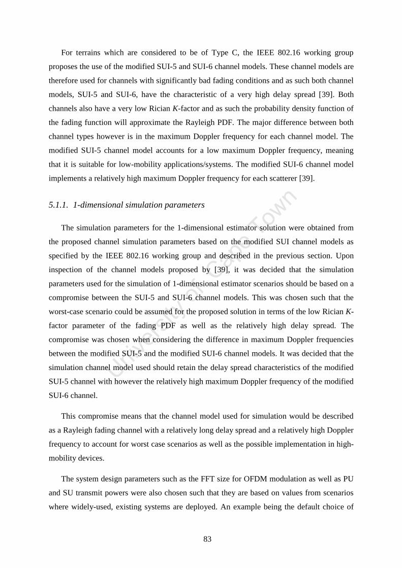
83

For terrains which are considered to be of Type C, the IEEE 802.16 working group

proposes the use of the modified SUI-5 and SUI-6 channel models. These channel models are

therefore used for channels with significantly bad fading conditions and as such both channel

models, SUI-5 and SUI-6, have the characteristic of a very high delay spread [39]. Both

channels also have a very low Rician K-factor and as such the probability density function of

the fading function will approximate the Rayleigh PDF. The major difference between both

channel types however is in the maximum Doppler frequency for each channel model. The

modified SUI-5 channel model accounts for a low maximum Doppler frequency, meaning

that it is suitable for low-mobility applications/systems. The modified SUI-6 channel model

implements a relatively high maximum Doppler frequency for each scatterer [39].

5.1.1. 1-dimensional simulation parameters

The simulation parameters for the 1-dimensional estimator solution were obtained from

the proposed channel simulation parameters based on the modified SUI channel models as

specified by the IEEE 802.16 working group and described in the previous section. Upon

inspection of the channel models proposed by [39], it was decided that the simulation

parameters used for the simulation of 1-dimensional estimator scenarios should be based on a

compromise between the SUI-5 and SUI-6 channel models. This was chosen such that the

worst-case scenario could be assumed for the proposed solution in terms of the low Rician K-

factor parameter of the fading PDF as well as the relatively high delay spread. The

compromise was chosen when considering the difference in maximum Doppler frequencies

between the modified SUI-5 and the modified SUI-6 channel models. It was decided that the

simulation channel model used should retain the delay spread characteristics of the modified

SUI-5 channel with however the relatively high maximum Doppler frequency of the modified

SUI-6 channel.

This compromise means that the channel model used for simulation would be described

as a Rayleigh fading channel with a relatively long delay spread and a relatively high Doppler

frequency to account for worst case scenarios as well as the possible implementation in high-

mobility devices.

The system design parameters such as the FFT size for OFDM modulation as well as PU

and SU transmit powers were also chosen such that they are based on values from scenarios

where widely-used, existing systems are deployed. An example being the default choice of

84

both PU and SU transmit powers being 20 dBm (100 mW) as this is the commonly used

power limit for the 2.4 GHz Industrial, Scientific and Medical (ISM) band as commonly used

by the IEEE 802.11 WiFi standard. Other parameters were also in generally chosen to

represent worst-case scenarios for the simulated communications device, for example, the

noise floor was chosen to be -90 dBm. More commonly, high-performance receivers have a

noise floor of less than -110 dBm and noise floors of -90 dBm are considered to be of a

poorly performing or designed receiver. The simulation parameters for the 1-dimensional

estimator scenario system simulations are therefore presented in Table 2.

Table 2. Simulation parameters for 1-dimensional estimator scenarios

Parameter Value

FFT Size 128

Noise Floor -90 dBm

OFDM Symbol Duration 288 µs

Sub-carrier Spacing 500 kHz

Cyclic Prefix 1/8 (ratio of OFDM symbol)

PU Bandwidths [4, 18, 36] sub-channels

Static Pilot Spacing (frequency) 9

Channel Fading PDF Rayleigh

PU Transmit Powers [0, 10, 20, 30] dBm

SU Transmit Power 20 dBm

Maximum Doppler Frequency 120 Hz

Channel Delay Spread 10 µs

Interference Thresholds [1, 3, 5, 7, 9, 10] mW

5.1.2. 2-dimensional simulation parameters

The simulation parameters for scenarios where a 2-dimensional estimator is employed by

the simulated CR devices were based on the simulation parameters of the 1-dimensional

estimator scenario. This is due to the fact that the extension from 1-dimensional to 2-

dimensional estimators is minimal in terms of system design and has no effect on the channel

model whatsoever.

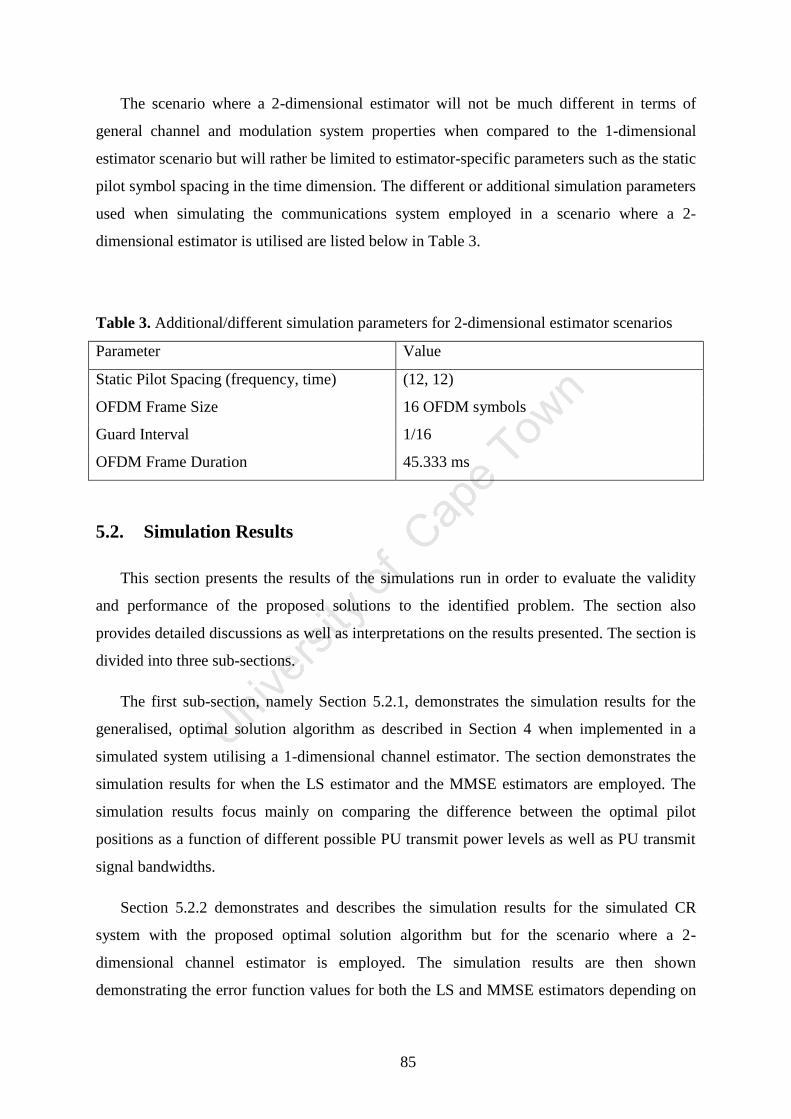
85

The scenario where a 2-dimensional estimator will not be much different in terms of

general channel and modulation system properties when compared to the 1-dimensional

estimator scenario but will rather be limited to estimator-specific parameters such as the static

pilot symbol spacing in the time dimension. The different or additional simulation parameters

used when simulating the communications system employed in a scenario where a 2-

dimensional estimator is utilised are listed below in Table 3.

Table 3. Additional/different simulation parameters for 2-dimensional estimator scenarios

Parameter Value

Static Pilot Spacing (frequency, time) (12, 12)

OFDM Frame Size 16 OFDM symbols

Guard Interval 1/16

OFDM Frame Duration 45.333 ms

5.2. Simulation Results

This section presents the results of the simulations run in order to evaluate the validity

and performance of the proposed solutions to the identified problem. The section also

provides detailed discussions as well as interpretations on the results presented. The section is

divided into three sub-sections.

The first sub-section, namely Section 5.2.1, demonstrates the simulation results for the

generalised, optimal solution algorithm as described in Section 4 when implemented in a

simulated system utilising a 1-dimensional channel estimator. The section demonstrates the

simulation results for when the LS estimator and the MMSE estimators are employed. The

simulation results focus mainly on comparing the difference between the optimal pilot

positions as a function of different possible PU transmit power levels as well as PU transmit

signal bandwidths.

Section 5.2.2 demonstrates and describes the simulation results for the simulated CR

system with the proposed optimal solution algorithm but for the scenario where a 2-

dimensional channel estimator is employed. The simulation results are then shown

demonstrating the error function values for both the LS and MMSE estimators depending on

86

different PU transmit signal powers as well as PU transmit signal bandwidths. This therefore

demonstrates how the algorithm obtains the optimal pilot patterns and a discussion is

developed for each figure demonstrating the usefulness and interpretation of the data in terms

of the performance and feasibility of the optimal solution algorithm. The section also quite

importantly shows how the optimal solution algorithm adapts when used in a 2-dimensional

estimator implementation by demonstrating the OFDM symbol MSE per OFDM symbol

while maintaining constant simulation system parameters such as PU transmit power and

bandwidth.

The last section, namely Section 5.3.3, allows the reader to compare the suitability of the

proposed sub-optimal solution schemes to the optimal solution schemes developed in terms

of accuracy as well as computational efficiency. Simulation results are shown comparing the

execution time and memory requirements of the optimal solution versus the proposed sub-

optimal algorithms, as demonstrated in Section 4.5, for both the LS and MMSE estimators.

The section also demonstrates how the computational complexity for the optimal, generalised

solution algorithm behaves when parameters of the simulated system (such as the FFT size

) are changed.

5.2.1. 1-dimensional, optimal solutions

This section presents the results of the optimal solution algorithm when applied for 1-

dimensional estimators as described in Section 4.2.1. The graphs presented below first

demonstrate the error function values for the cases when a LS estimator (Section 5.2.1.1) is

utilised followed by graphs which demonstrate the error function values when a MMSE

(Section 5.2.1.2) estimator is used.

The results shown in this sub-section serve to demonstrate the error function values,

equivalent to the heuristic function values for the 1-dimensional estimator case, of the 1-

dimensional optimal solution algorithm. This is done so that the reader may easily interpret

the way the algorithm works on the most basic level before making decisions (i.e., picking

the candidate pilot positions with the lowest error function value).

5.2.1.1. Least-squares estimator

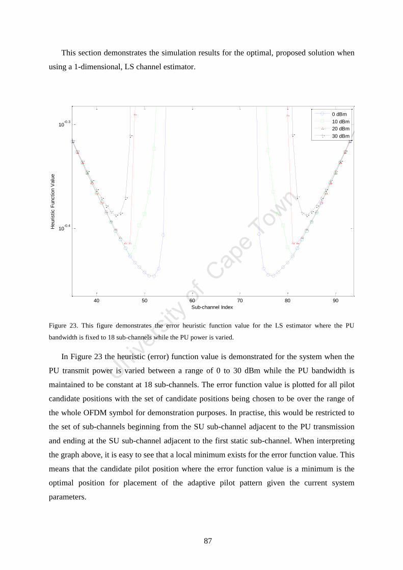
87

This section demonstrates the simulation results for the optimal, proposed solution when

using a 1-dimensional, LS channel estimator.

Figure 23. This figure demonstrates the error heuristic function value for the LS estimator where the PU

bandwidth is fixed to 18 sub-channels while the PU power is varied.

In Figure 23 the heuristic (error) function value is demonstrated for the system when the

PU transmit power is varied between a range of 0 to 30 dBm while the PU bandwidth is

maintained to be constant at 18 sub-channels. The error function value is plotted for all pilot

candidate positions with the set of candidate positions being chosen to be over the range of

the whole OFDM symbol for demonstration purposes. In practise, this would be restricted to

the set of sub-channels beginning from the SU sub-channel adjacent to the PU transmission

and ending at the SU sub-channel adjacent to the first static sub-channel. When interpreting

the graph above, it is easy to see that a local minimum exists for the error function value. This

means that the candidate pilot position where the error function value is a minimum is the

optimal position for placement of the adaptive pilot pattern given the current system

parameters.

40 50 60 70 80 90

10-0.4

10-0.3

Sub-channel Index

Heuristic F

unction V

alu

e

0 dBm

10 dBm

20 dBm

30 dBm

88

It is vital to note in Figure 23 above how steeply the error function value increases as the

sub-channels approach the PU transmission band. This is due to the fact that the optimal

power loading algorithm loads an almost (and in the case of some sub-channels, exactly) no

power to those sub-channels, meaning that the estimates at those points will be either

extremely noisy/inaccurate or in the case of no power loaded to those sub-channels, no

estimates may be done at all in those positions, meaning that those sub-channels are

effectively disabled. Another important aspect to note is how the area where zero power is

loaded to the SU sub-channels increases as the PU transmission power increases as well. This

is due to the increased interference from the spectral roll-off of the PU's pulse-shaping filter

being introduced to the SU's sub-channels. As such, the error function value minima are

farther away from the PU transmission as the PU's transmit power increases.

The aspect of increasing error function values as a function of PU transmit power as

shown above also gives rise to another curious phenomenon where the value of the minimum

itself is higher as the PU transmit power increases. This means that the optimal pilot

candidate positions for each different PU transmit power provide worse estimates in terms of

the overall estimator MSE for scenarios where there are higher PU transmit powers. This may

be attributed to the extra amount of noise attributed to the SU sub-channels near to the PU but

also to the increased distance between the candidate pilot positions and the PU band due to

the larger set of unusable sub-channels due to the power loading algorithm and the increased

PU transmission power.

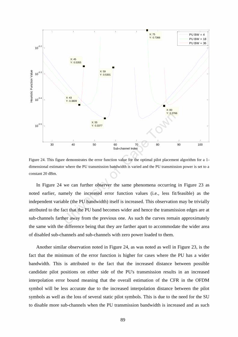
89

Figure 24. This figure demonstrates the error function value for the optimal pilot placement algorithm for a 1-

dimensional estimator where the PU transmission bandwidth is varied and the PU transmission power is set to a

constant 20 dBm.

In Figure 24 we can further observer the same phenomena occurring in Figure 23 as

noted earlier, namely the increased error function values (i.e., less fit/feasible) as the

independent variable (the PU bandwidth) itself is increased. This observation may be trivially

attributed to the fact that the PU band becomes wider and hence the transmission edges are at

sub-channels farther away from the previous one. As such the curves remain approximately

the same with the difference being that they are farther apart to accommodate the wider area

of disabled sub-channels and sub-channels with zero power loaded to them.

Another similar observation noted in Figure 24, as was noted as well in Figure 23, is the

fact that the minimum of the error function is higher for cases where the PU has a wider

bandwidth. This is attributed to the fact that the increased distance between possible

candidate pilot positions on either side of the PU's transmission results in an increased

interpolation error bound meaning that the overall estimation of the CFR in the OFDM

symbol will be less accurate due to the increased interpolation distance between the pilot

symbols as well as the loss of several static pilot symbols. This is due to the need for the SU

to disable more sub-channels when the PU transmission bandwidth is increased and as such

30 40 50 60 70 80 90 100

10-0.5

10-0.4

10-0.3

10-0.2

X: 83

Y: 0.3766

Sub-channel Index

Heuristic F

unction V

alu

e

X: 43

Y: 0.3809

X: 45

Y: 0.5355

X: 75

Y: 0.7366

X: 55

Y: 0.3377

X: 59

Y: 0.5301

PU BW = 4

PU BW = 18

PU BW = 36

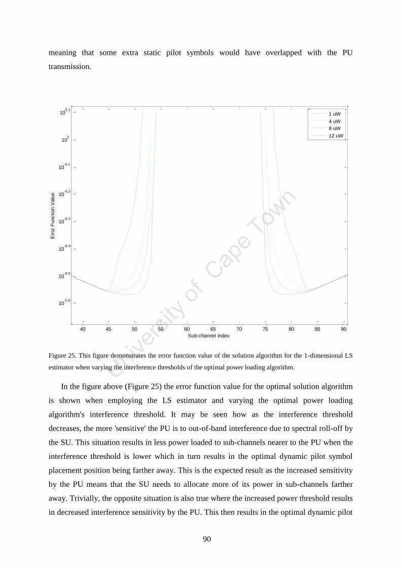
90

meaning that some extra static pilot symbols would have overlapped with the PU

transmission.

Figure 25. This figure demonstrates the error function value of the solution algorithm for the 1-dimensional LS

estimator when varying the interference thresholds of the optimal power loading algorithm.

In the figure above (Figure 25) the error function value for the optimal solution algorithm

is shown when employing the LS estimator and varying the optimal power loading

algorithm's interference threshold. It may be seen how as the interference threshold

decreases, the more 'sensitive' the PU is to out-of-band interference due to spectral roll-off by

the SU. This situation results in less power loaded to sub-channels nearer to the PU when the

interference threshold is lower which in turn results in the optimal dynamic pilot symbol

placement position being farther away. This is the expected result as the increased sensitivity

by the PU means that the SU needs to allocate more of its power in sub-channels farther

away. Trivially, the opposite situation is also true where the increased power threshold results

in decreased interference sensitivity by the PU. This then results in the optimal dynamic pilot

40 45 50 55 60 65 70 75 80 85 90

10-0.6

10-0.5

10-0.4

10-0.3

10-0.2

10-0.1

100

100.1

Sub-channel Index

Err

or

Function V

alu

e

1 uW

4 uW

8 uW

12 uW

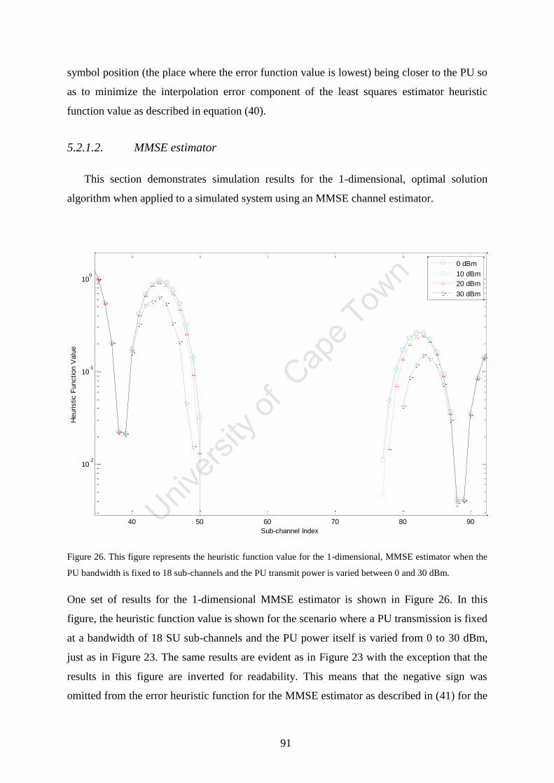
91

symbol position (the place where the error function value is lowest) being closer to the PU so

as to minimize the interpolation error component of the least squares estimator heuristic

function value as described in equation (40).

5.2.1.2. MMSE estimator

This section demonstrates simulation results for the 1-dimensional, optimal solution

algorithm when applied to a simulated system using an MMSE channel estimator.

Figure 26. This figure represents the heuristic function value for the 1-dimensional, MMSE estimator when the

PU bandwidth is fixed to 18 sub-channels and the PU transmit power is varied between 0 and 30 dBm.

One set of results for the 1-dimensional MMSE estimator is shown in Figure 26. In this

figure, the heuristic function value is shown for the scenario where a PU transmission is fixed

at a bandwidth of 18 SU sub-channels and the PU power itself is varied from 0 to 30 dBm,

just as in Figure 23. The same results are evident as in Figure 23 with the exception that the

results in this figure are inverted for readability. This means that the negative sign was

omitted from the error heuristic function for the MMSE estimator as described in (41) for the

40 50 60 70 80 90

10-2

10-1

100

Sub-channel Index

Heuristic F

unction V

alu

e

0 dBm

10 dBm

20 dBm

30 dBm

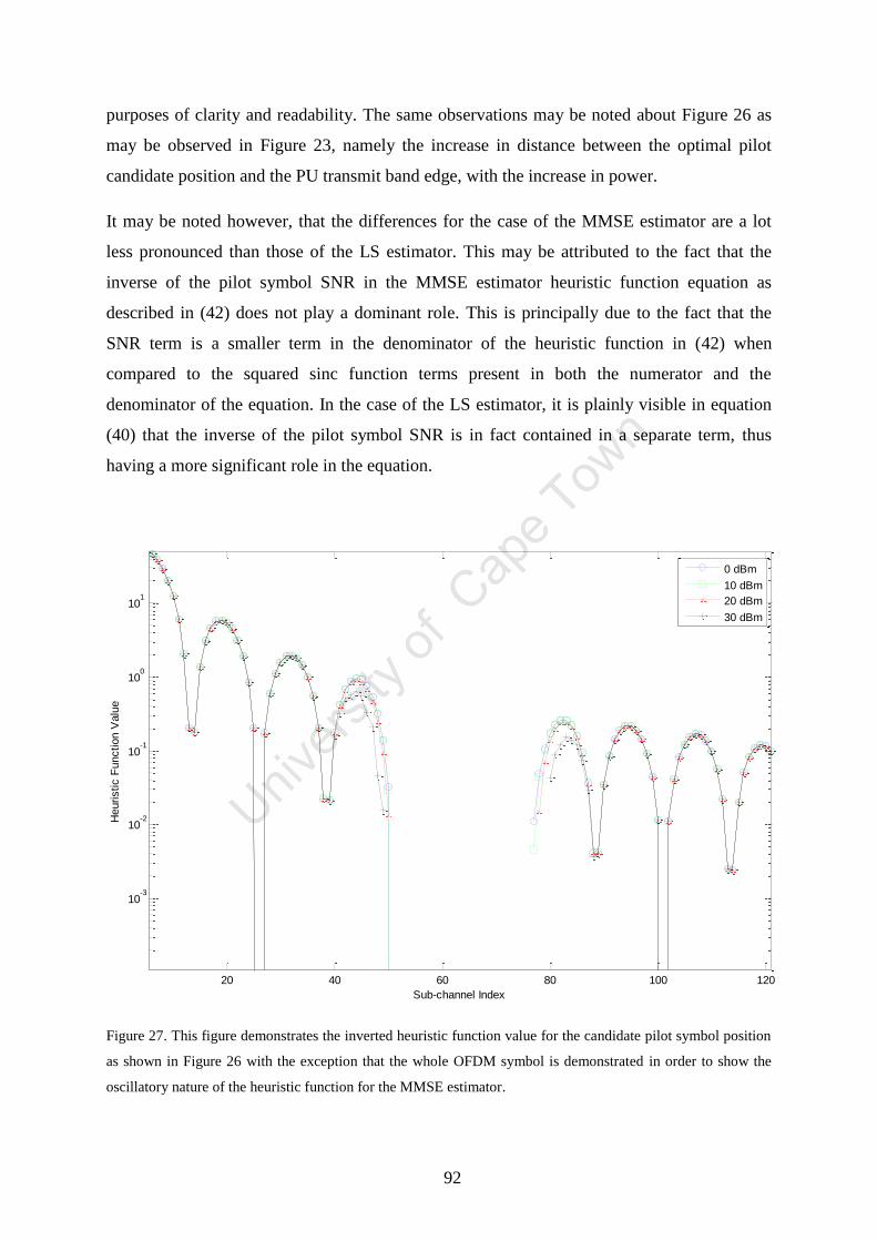
92

purposes of clarity and readability. The same observations may be noted about Figure 26 as

may be observed in Figure 23, namely the increase in distance between the optimal pilot

candidate position and the PU transmit band edge, with the increase in power.

It may be noted however, that the differences for the case of the MMSE estimator are a lot

less pronounced than those of the LS estimator. This may be attributed to the fact that the

inverse of the pilot symbol SNR in the MMSE estimator heuristic function equation as

described in (42) does not play a dominant role. This is principally due to the fact that the

SNR term is a smaller term in the denominator of the heuristic function in (42) when

compared to the squared sinc function terms present in both the numerator and the

denominator of the equation. In the case of the LS estimator, it is plainly visible in equation

(40) that the inverse of the pilot symbol SNR is in fact contained in a separate term, thus

having a more significant role in the equation.

Figure 27. This figure demonstrates the inverted heuristic function value for the candidate pilot symbol position

as shown in Figure 26 with the exception that the whole OFDM symbol is demonstrated in order to show the

oscillatory nature of the heuristic function for the MMSE estimator.

20 40 60 80 100 120

10-3

10-2

10-1

100

101

Sub-channel Index

Heuristic F

unction V

alu

e

0 dBm

10 dBm

20 dBm

30 dBm

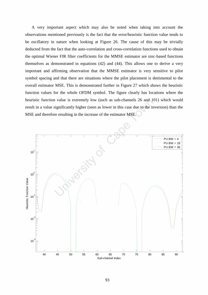
93

A very important aspect which may also be noted when taking into account the

observations mentioned previously is the fact that the error/heuristic function value tends to

be oscillatory in nature when looking at Figure 26. The cause of this may be trivially

deducted from the fact that the auto-correlation and cross-correlation functions used to obtain

the optimal Wiener FIR filter coefficients for the MMSE estimator are sinc-based functions

themselves as demonstrated in equations (42) and (44). This allows one to derive a very

important and affirming observation that the MMSE estimator is very sensitive to pilot

symbol spacing and that there are situations where the pilot placement is detrimental to the

overall estimator MSE. This is demonstrated further in Figure 27 which shows the heuristic

function values for the whole OFDM symbol. The figure clearly has locations where the

heuristic function value is extremely low (such as sub-channels 26 and 101) which would

result in a value significantly higher (seen as lower in this case due to the inversion) than the

MSE and therefore resulting in the increase of the estimator MSE.

40 45 50 55 60 65 70 75 80 85 90

10-3

10-2

10-1

100

101

Sub-channel Index

Heuristic F

unction V

alu

e

PU BW = 4

PU BW = 18

PU BW = 36

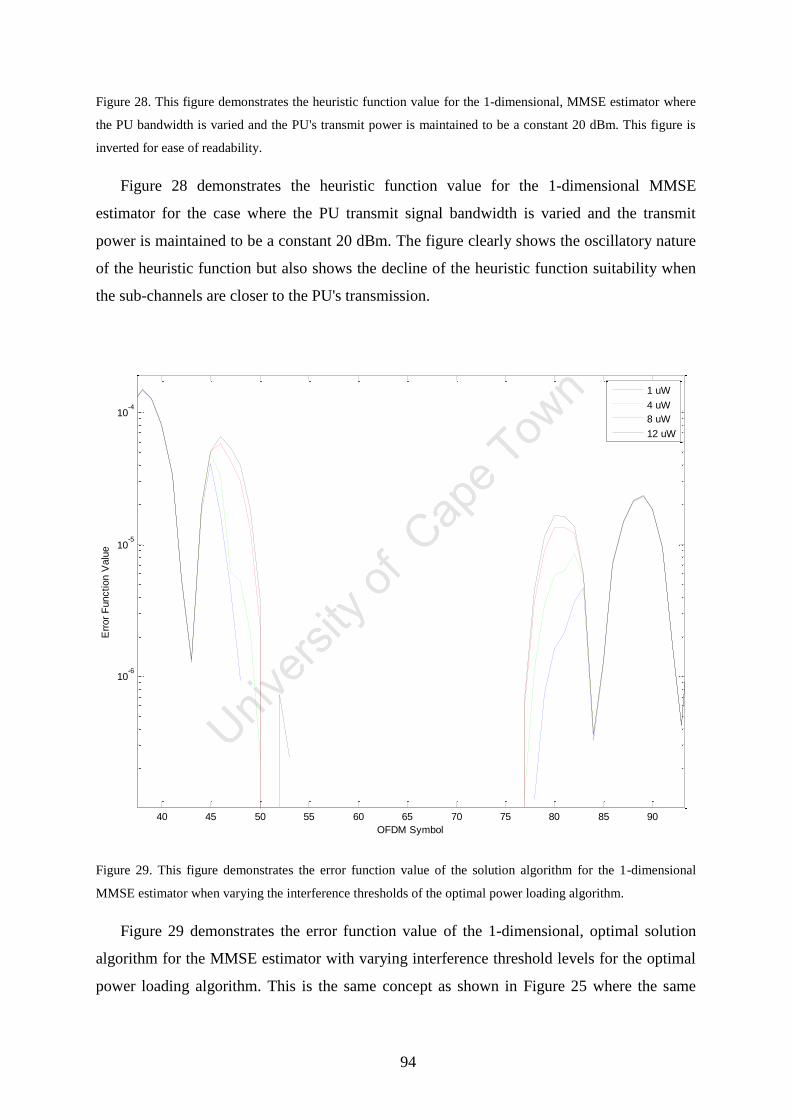
94

Figure 28. This figure demonstrates the heuristic function value for the 1-dimensional, MMSE estimator where

the PU bandwidth is varied and the PU's transmit power is maintained to be a constant 20 dBm. This figure is

inverted for ease of readability.

Figure 28 demonstrates the heuristic function value for the 1-dimensional MMSE

estimator for the case where the PU transmit signal bandwidth is varied and the transmit

power is maintained to be a constant 20 dBm. The figure clearly shows the oscillatory nature

of the heuristic function but also shows the decline of the heuristic function suitability when

the sub-channels are closer to the PU's transmission.

Figure 29. This figure demonstrates the error function value of the solution algorithm for the 1-dimensional

MMSE estimator when varying the interference thresholds of the optimal power loading algorithm.

Figure 29 demonstrates the error function value of the 1-dimensional, optimal solution

algorithm for the MMSE estimator with varying interference threshold levels for the optimal

power loading algorithm. This is the same concept as shown in Figure 25 where the same

40 45 50 55 60 65 70 75 80 85 90

10-6

10-5

10-4

OFDM Symbol

Err

or

Function V

alu

e

1 uW

4 uW

8 uW

12 uW

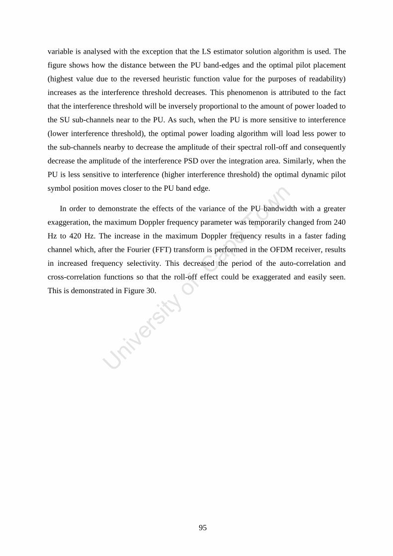
95

variable is analysed with the exception that the LS estimator solution algorithm is used. The

figure shows how the distance between the PU band-edges and the optimal pilot placement

(highest value due to the reversed heuristic function value for the purposes of readability)

increases as the interference threshold decreases. This phenomenon is attributed to the fact

that the interference threshold will be inversely proportional to the amount of power loaded to

the SU sub-channels near to the PU. As such, when the PU is more sensitive to interference

(lower interference threshold), the optimal power loading algorithm will load less power to

the sub-channels nearby to decrease the amplitude of their spectral roll-off and consequently

decrease the amplitude of the interference PSD over the integration area. Similarly, when the

PU is less sensitive to interference (higher interference threshold) the optimal dynamic pilot

symbol position moves closer to the PU band edge.

In order to demonstrate the effects of the variance of the PU bandwidth with a greater

exaggeration, the maximum Doppler frequency parameter was temporarily changed from 240

Hz to 420 Hz. The increase in the maximum Doppler frequency results in a faster fading

channel which, after the Fourier (FFT) transform is performed in the OFDM receiver, results

in increased frequency selectivity. This decreased the period of the auto-correlation and

cross-correlation functions so that the roll-off effect could be exaggerated and easily seen.

This is demonstrated in Figure 30.

96

Figure 30. This figure demonstrates the heuristic function value per sub-channel as done in Figure 28 with the

exception that the maximum Doppler frequency is increased to 420 Hz so as to allow an easier demonstration of

the spectral roll-off effect.

A very interesting observation which can be deduced from the figures shown above is

how the heuristic function value seems to be better (lower for LS or higher when inverted for

the MMSE estimator graphs) for sub-channels farther away from the PU when the PU

bandwidth is increased. Conversely, the heuristic function value seems to be worse (higher

for the LS estimator and lower for the MMSE estimator due to the inverted graphs) for sub-

channels nearer to the PU when the PU bandwidth is increased. This observation may be

attributed to the optimal power loading algorithm. Since for cases where the PU transmission

bandwidth is higher there are less SU sub-channels to which the same total power needs to be

allocated to. This is necessary so as to maximise the channel capacity for the modulation

scheme of use. This means that for cases where the PU bandwidth is higher, there will be a

greater difference between the amounts of power loaded to adjacent sub-channels than for

cases where the PU transmission bandwidth is lower. As such, this results in a steeper

gradient of power loading so as to ensure that the sum of the power loaded to all SU sub-

channels (the total SU transmission power) still remains as high as possible without

exceeding the interference threshold. As such, channels farther away will have more power

45 50 55 60 65 70 75 80 85

10-3

10-2

10-1

Sub-channel Index

Heuristic F

unction V

alu

e

PU BW = 4

PU BW = 18

PU BW = 36

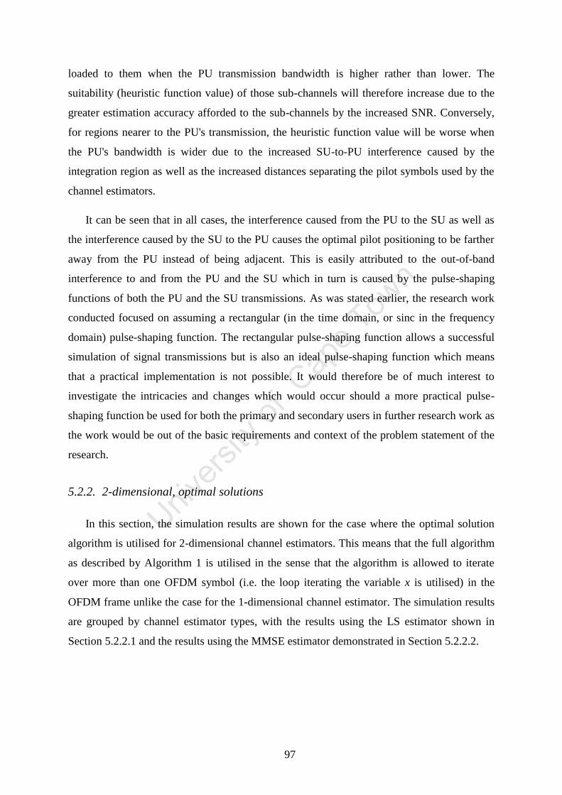
97

loaded to them when the PU transmission bandwidth is higher rather than lower. The

suitability (heuristic function value) of those sub-channels will therefore increase due to the

greater estimation accuracy afforded to the sub-channels by the increased SNR. Conversely,

for regions nearer to the PU's transmission, the heuristic function value will be worse when

the PU's bandwidth is wider due to the increased SU-to-PU interference caused by the

integration region as well as the increased distances separating the pilot symbols used by the

channel estimators.

It can be seen that in all cases, the interference caused from the PU to the SU as well as

the interference caused by the SU to the PU causes the optimal pilot positioning to be farther

away from the PU instead of being adjacent. This is easily attributed to the out-of-band

interference to and from the PU and the SU which in turn is caused by the pulse-shaping

functions of both the PU and the SU transmissions. As was stated earlier, the research work

conducted focused on assuming a rectangular (in the time domain, or sinc in the frequency

domain) pulse-shaping function. The rectangular pulse-shaping function allows a successful

simulation of signal transmissions but is also an ideal pulse-shaping function which means

that a practical implementation is not possible. It would therefore be of much interest to

investigate the intricacies and changes which would occur should a more practical pulse-

shaping function be used for both the primary and secondary users in further research work as

the work would be out of the basic requirements and context of the problem statement of the

research.

5.2.2. 2-dimensional, optimal solutions

In this section, the simulation results are shown for the case where the optimal solution

algorithm is utilised for 2-dimensional channel estimators. This means that the full algorithm

as described by Algorithm 1 is utilised in the sense that the algorithm is allowed to iterate

over more than one OFDM symbol (i.e. the loop iterating the variable x is utilised) in the

OFDM frame unlike the case for the 1-dimensional channel estimator. The simulation results

are grouped by channel estimator types, with the results using the LS estimator shown in

Section 5.2.2.1 and the results using the MMSE estimator demonstrated in Section 5.2.2.2.

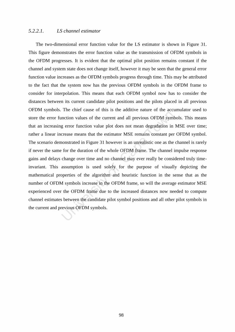
98

5.2.2.1. LS channel estimator

The two-dimensional error function value for the LS estimator is shown in Figure 31.

This figure demonstrates the error function value as the transmission of OFDM symbols in

the OFDM progresses. It is evident that the optimal pilot position remains constant if the

channel and system state does not change itself, however it may be seen that the general error

function value increases as the OFDM symbols progress through time. This may be attributed

to the fact that the system now has the previous OFDM symbols in the OFDM frame to

consider for interpolation. This means that each OFDM symbol now has to consider the

distances between its current candidate pilot positions and the pilots placed in all previous

OFDM symbols. The chief cause of this is the additive nature of the accumulator used to

store the error function values of the current and all previous OFDM symbols. This means

that an increasing error function value plot does not mean degradation in MSE over time;

rather a linear increase means that the estimator MSE remains constant per OFDM symbol.

The scenario demonstrated in Figure 31 however is an unrealistic one as the channel is rarely

if never the same for the duration of the whole OFDM frame. The channel impulse response

gains and delays change over time and no channel may ever really be considered truly time-

invariant. This assumption is used solely for the purpose of visually depicting the

mathematical properties of the algorithm and heuristic function in the sense that as the

number of OFDM symbols increase in the OFDM frame, so will the average estimator MSE

experienced over the OFDM frame due to the increased distances now needed to compute

channel estimates between the candidate pilot symbol positions and all other pilot symbols in

the current and previous OFDM symbols.

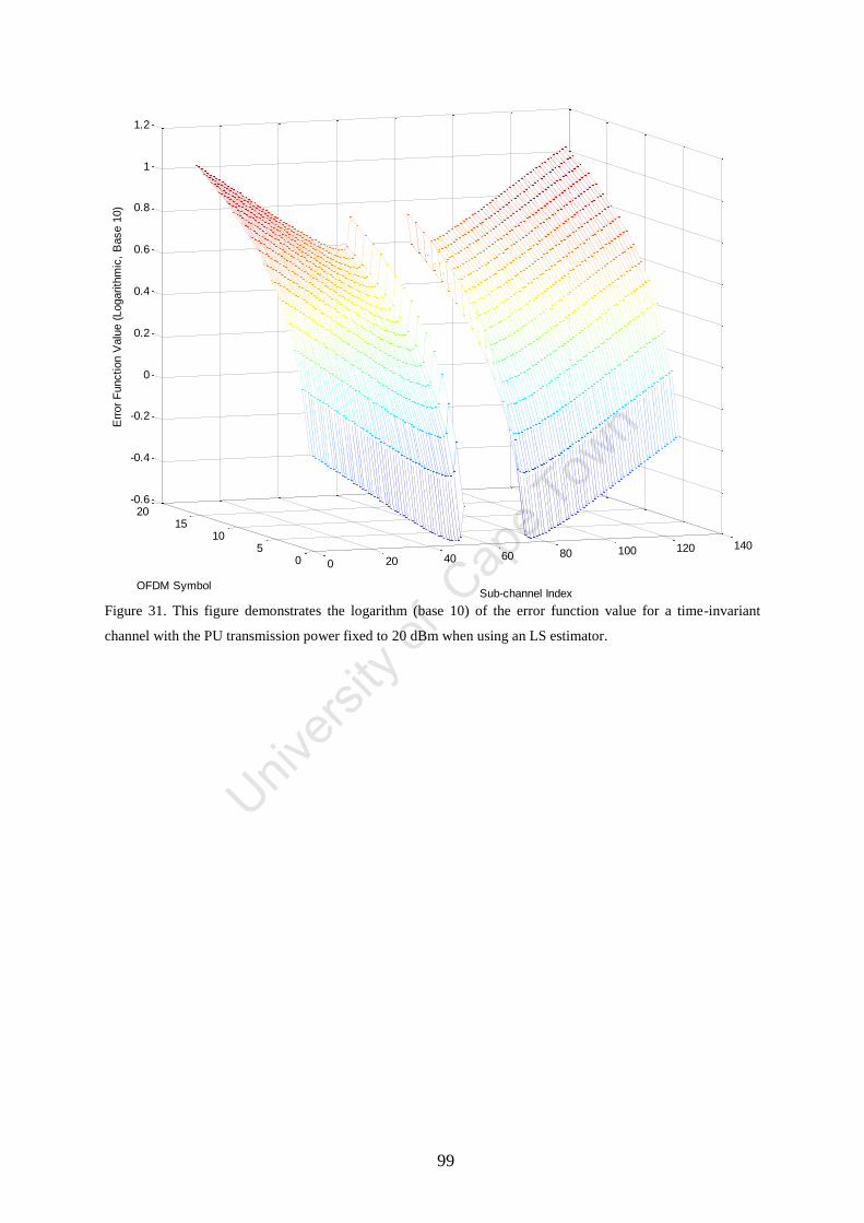
99

Figure 31. This figure demonstrates the logarithm (base 10) of the error function value for a time-invariant

channel with the PU transmission power fixed to 20 dBm when using an LS estimator.

0 20 40 60 80 100 120 140

05

1015

20-0.6

-0.4

-0.2

0

0.2

0.4

0.6

0.8

1

1.2

Sub-channel IndexOFDM Symbol

Err

or

Function V

alu

e (

Logarith

mic

, B

ase 1

0)

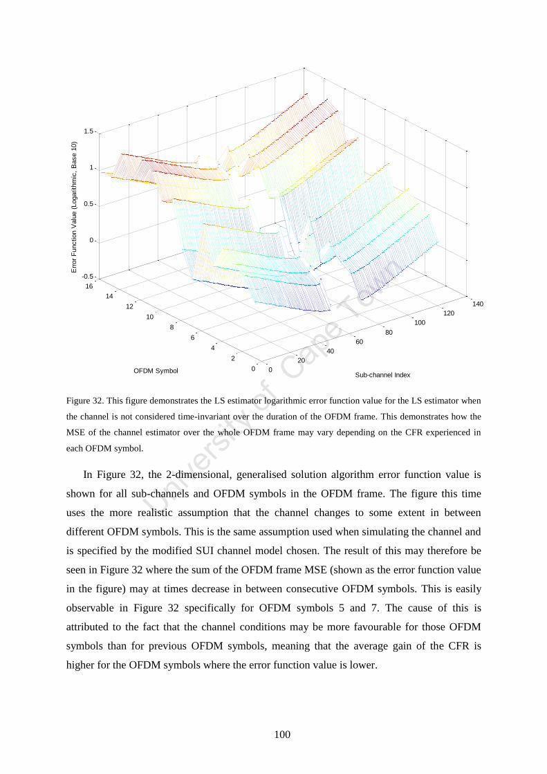
100

Figure 32. This figure demonstrates the LS estimator logarithmic error function value for the LS estimator when

the channel is not considered time-invariant over the duration of the OFDM frame. This demonstrates how the

MSE of the channel estimator over the whole OFDM frame may vary depending on the CFR experienced in

each OFDM symbol.

In Figure 32, the 2-dimensional, generalised solution algorithm error function value is

shown for all sub-channels and OFDM symbols in the OFDM frame. The figure this time

uses the more realistic assumption that the channel changes to some extent in between

different OFDM symbols. This is the same assumption used when simulating the channel and

is specified by the modified SUI channel model chosen. The result of this may therefore be

seen in Figure 32 where the sum of the OFDM frame MSE (shown as the error function value

in the figure) may at times decrease in between consecutive OFDM symbols. This is easily

observable in Figure 32 specifically for OFDM symbols 5 and 7. The cause of this is

attributed to the fact that the channel conditions may be more favourable for those OFDM

symbols than for previous OFDM symbols, meaning that the average gain of the CFR is

higher for the OFDM symbols where the error function value is lower.

0

20

40

60

80

100

120

140

0

2

4

6

8

10

12

14

16

-0.5

0

0.5

1

1.5

Sub-channel IndexOFDM Symbol

Err

or

Function V

alu

e (

Logarith

mic

, B

ase 1

0)

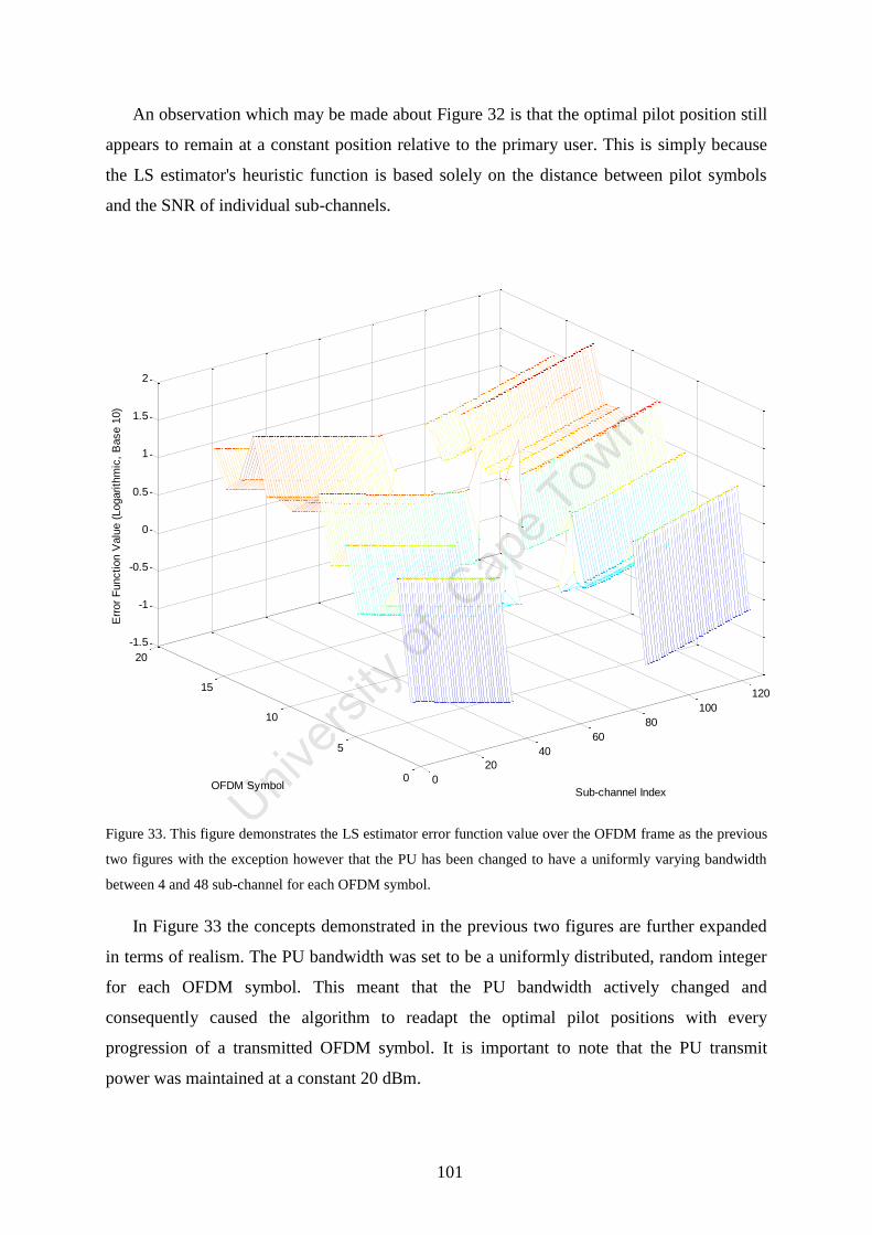
101

An observation which may be made about Figure 32 is that the optimal pilot position still

appears to remain at a constant position relative to the primary user. This is simply because

the LS estimator's heuristic function is based solely on the distance between pilot symbols

and the SNR of individual sub-channels.

Figure 33. This figure demonstrates the LS estimator error function value over the OFDM frame as the previous

two figures with the exception however that the PU has been changed to have a uniformly varying bandwidth

between 4 and 48 sub-channel for each OFDM symbol.

In Figure 33 the concepts demonstrated in the previous two figures are further expanded

in terms of realism. The PU bandwidth was set to be a uniformly distributed, random integer

for each OFDM symbol. This meant that the PU bandwidth actively changed and

consequently caused the algorithm to readapt the optimal pilot positions with every

progression of a transmitted OFDM symbol. It is important to note that the PU transmit

power was maintained at a constant 20 dBm.

0

20

40

60

80

100

120

0

5

10

15

20

-1.5

-1

-0.5

0

0.5

1

1.5

2

Sub-channel IndexOFDM Symbol

Err

or

Function V

alu

e (

Logarith

mic

, B

ase 1

0)

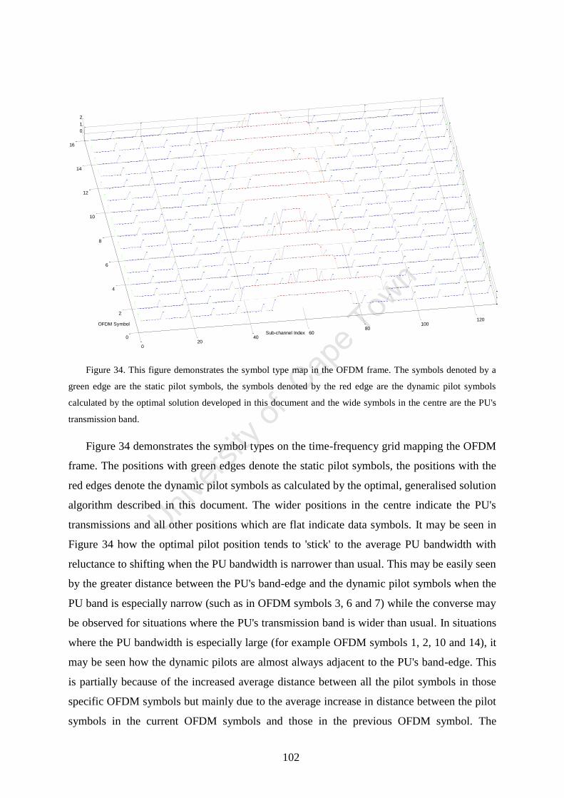
102

Figure 34. This figure demonstrates the symbol type map in the OFDM frame. The symbols denoted by a

green edge are the static pilot symbols, the symbols denoted by the red edge are the dynamic pilot symbols

calculated by the optimal solution developed in this document and the wide symbols in the centre are the PU's

transmission band.

Figure 34 demonstrates the symbol types on the time-frequency grid mapping the OFDM

frame. The positions with green edges denote the static pilot symbols, the positions with the

red edges denote the dynamic pilot symbols as calculated by the optimal, generalised solution

algorithm described in this document. The wider positions in the centre indicate the PU's

transmissions and all other positions which are flat indicate data symbols. It may be seen in

Figure 34 how the optimal pilot position tends to 'stick' to the average PU bandwidth with

reluctance to shifting when the PU bandwidth is narrower than usual. This may be easily seen

by the greater distance between the PU's band-edge and the dynamic pilot symbols when the

PU band is especially narrow (such as in OFDM symbols 3, 6 and 7) while the converse may

be observed for situations where the PU's transmission band is wider than usual. In situations

where the PU bandwidth is especially large (for example OFDM symbols 1, 2, 10 and 14), it

may be seen how the dynamic pilots are almost always adjacent to the PU's band-edge. This

is partially because of the increased average distance between all the pilot symbols in those

specific OFDM symbols but mainly due to the average increase in distance between the pilot

symbols in the current OFDM symbols and those in the previous OFDM symbol. The

020

4060

80100

120

0

2

4

6

8

10

12

14

16

0

1

2

Sub-channel Index

OFDM Symbol

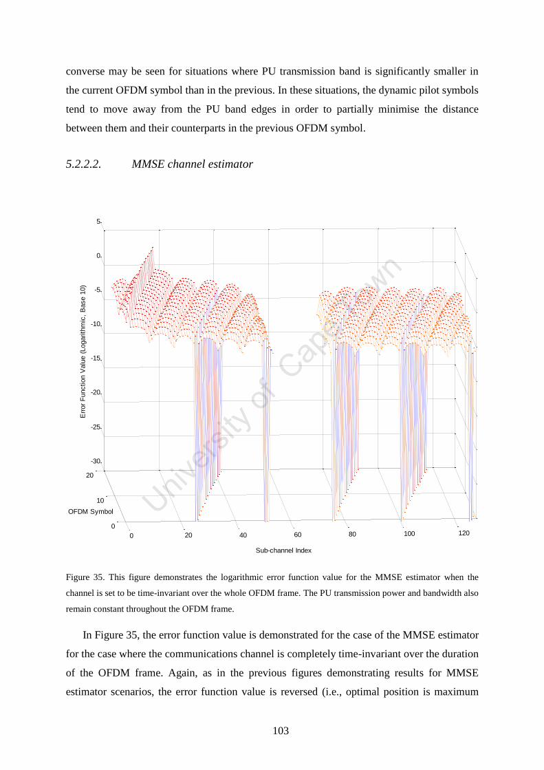
103

converse may be seen for situations where PU transmission band is significantly smaller in

the current OFDM symbol than in the previous. In these situations, the dynamic pilot symbols

tend to move away from the PU band edges in order to partially minimise the distance

between them and their counterparts in the previous OFDM symbol.

5.2.2.2. MMSE channel estimator

Figure 35. This figure demonstrates the logarithmic error function value for the MMSE estimator when the

channel is set to be time-invariant over the whole OFDM frame. The PU transmission power and bandwidth also

remain constant throughout the OFDM frame.

In Figure 35, the error function value is demonstrated for the case of the MMSE estimator

for the case where the communications channel is completely time-invariant over the duration

of the OFDM frame. Again, as in the previous figures demonstrating results for MMSE

estimator scenarios, the error function value is reversed (i.e., optimal position is maximum

0 20 40 60 80 100 1200

10

20

-30

-25

-20

-15

-10

-5

0

5

Sub-channel Index

OFDM Symbol

Err

or

Function V

alu

e (

Logarith

mic

, B

ase 1

0)

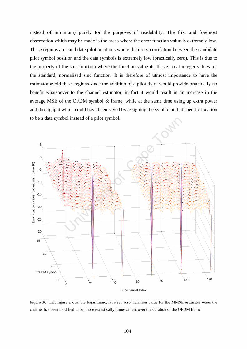
104

instead of minimum) purely for the purposes of readability. The first and foremost

observation which may be made is the areas where the error function value is extremely low.

These regions are candidate pilot positions where the cross-correlation between the candidate

pilot symbol position and the data symbols is extremely low (practically zero). This is due to

the property of the sinc function where the function value itself is zero at integer values for

the standard, normalised sinc function. It is therefore of utmost importance to have the

estimator avoid these regions since the addition of a pilot there would provide practically no

benefit whatsoever to the channel estimator, in fact it would result in an increase in the

average MSE of the OFDM symbol & frame, while at the same time using up extra power

and throughput which could have been saved by assigning the symbol at that specific location

to be a data symbol instead of a pilot symbol.

Figure 36. This figure shows the logarithmic, reversed error function value for the MMSE estimator when the

channel has been modified to be, more realistically, time-variant over the duration of the OFDM frame.

0 20 40 60 80 100 1200

5

10

15

-30

-25

-20

-15

-10

-5

0

5

Sub-channel Index

OFDM symbol

Err

or

Function V

alu

e (

Logarith

mic

, B

ase 1

0)

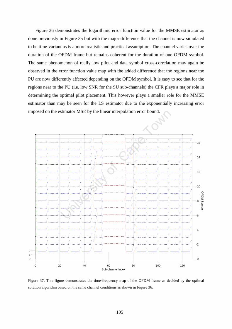
105

Figure 36 demonstrates the logarithmic error function value for the MMSE estimator as

done previously in Figure 35 but with the major difference that the channel is now simulated

to be time-variant as is a more realistic and practical assumption. The channel varies over the

duration of the OFDM frame but remains coherent for the duration of one OFDM symbol.

The same phenomenon of really low pilot and data symbol cross-correlation may again be

observed in the error function value map with the added difference that the regions near the

PU are now differently affected depending on the OFDM symbol. It is easy to see that for the

regions near to the PU (i.e. low SNR for the SU sub-channels) the CFR plays a major role in

determining the optimal pilot placement. This however plays a smaller role for the MMSE

estimator than may be seen for the LS estimator due to the exponentially increasing error

imposed on the estimator MSE by the linear interpolation error bound.

Figure 37. This figure demonstrates the time-frequency map of the OFDM frame as decided by the optimal

solution algorithm based on the same channel conditions as shown in Figure 36.

0 20 40 60 80 100 120

0

2

4

6

8

10

12

14

16

0

1

2

OF

DM

Sym

bol

Sub-channel Index

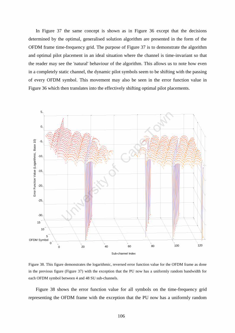
106

In Figure 37 the same concept is shown as in Figure 36 except that the decisions

determined by the optimal, generalised solution algorithm are presented in the form of the

OFDM frame time-frequency grid. The purpose of Figure 37 is to demonstrate the algorithm

and optimal pilot placement in an ideal situation where the channel is time-invariant so that

the reader may see the 'natural' behaviour of the algorithm. This allows us to note how even

in a completely static channel, the dynamic pilot symbols seem to be shifting with the passing

of every OFDM symbol. This movement may also be seen in the error function value in

Figure 36 which then translates into the effectively shifting optimal pilot placements.

Figure 38. This figure demonstrates the logarithmic, reversed error function value for the OFDM frame as done

in the previous figure (Figure 37) with the exception that the PU now has a uniformly random bandwidth for

each OFDM symbol between 4 and 48 SU sub-channels.

Figure 38 shows the error function value for all symbols on the time-frequency grid

representing the OFDM frame with the exception that the PU now has a uniformly random

0 20 40 60 80 100 1200

5

10

15

-30

-25

-20

-15

-10

-5

0

5

Sub-channel Index

OFDM Symbol

Err

or

Function V

alu

e (

Logarith

mic

, B

ase 1

0)

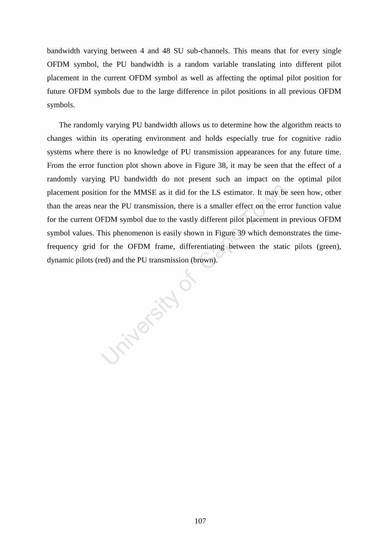
107

bandwidth varying between 4 and 48 SU sub-channels. This means that for every single

OFDM symbol, the PU bandwidth is a random variable translating into different pilot

placement in the current OFDM symbol as well as affecting the optimal pilot position for

future OFDM symbols due to the large difference in pilot positions in all previous OFDM

symbols.

The randomly varying PU bandwidth allows us to determine how the algorithm reacts to

changes within its operating environment and holds especially true for cognitive radio

systems where there is no knowledge of PU transmission appearances for any future time.

From the error function plot shown above in Figure 38, it may be seen that the effect of a

randomly varying PU bandwidth do not present such an impact on the optimal pilot

placement position for the MMSE as it did for the LS estimator. It may be seen how, other

than the areas near the PU transmission, there is a smaller effect on the error function value

for the current OFDM symbol due to the vastly different pilot placement in previous OFDM

symbol values. This phenomenon is easily shown in Figure 39 which demonstrates the time-

frequency grid for the OFDM frame, differentiating between the static pilots (green),

dynamic pilots (red) and the PU transmission (brown).

108

Figure 39. This figure demonstrates the OFDM frame time-frequency grid as decided by the optimal solution

algorithm for the same conditions as demonstrated in Figure 38.

As shown previously in Figure 34 demonstrating the time-frequency grid for the LS

estimator, the effect of the solution algorithm placing pilots closer to the PU transmission in

the current OFDM symbol if follow an OFDM symbol with a wider PU bandwidth, or

effectively the 'reluctance' to deviation, of the solution algorithm may not be seen for the

MMSE estimator. The optimal pilot symbols seem to be more 'independent' of each other for

the MMSE scenario due to the much smaller impact distances between pilot and data symbols

make for the MMSE estimator compared to the error bounds for the linear interpolator in the

LS estimator. This reiterates the common practise of employing LS estimators for channels

which have a CIR with less taps, and hence providing a more linear CFR, so as to take

advantage of the reduced complexity of the LS estimator implementation. On the other hand,

the MMSE estimator error function value shows how the MMSE estimator is a better choice

for channels with more complicated CFRs and hence more resolvable taps in the CIR.

020

4060

80100

120

0

2

4

6

8

10

12

14

16

01

2

Sub-channel IndexOFDM Symbol

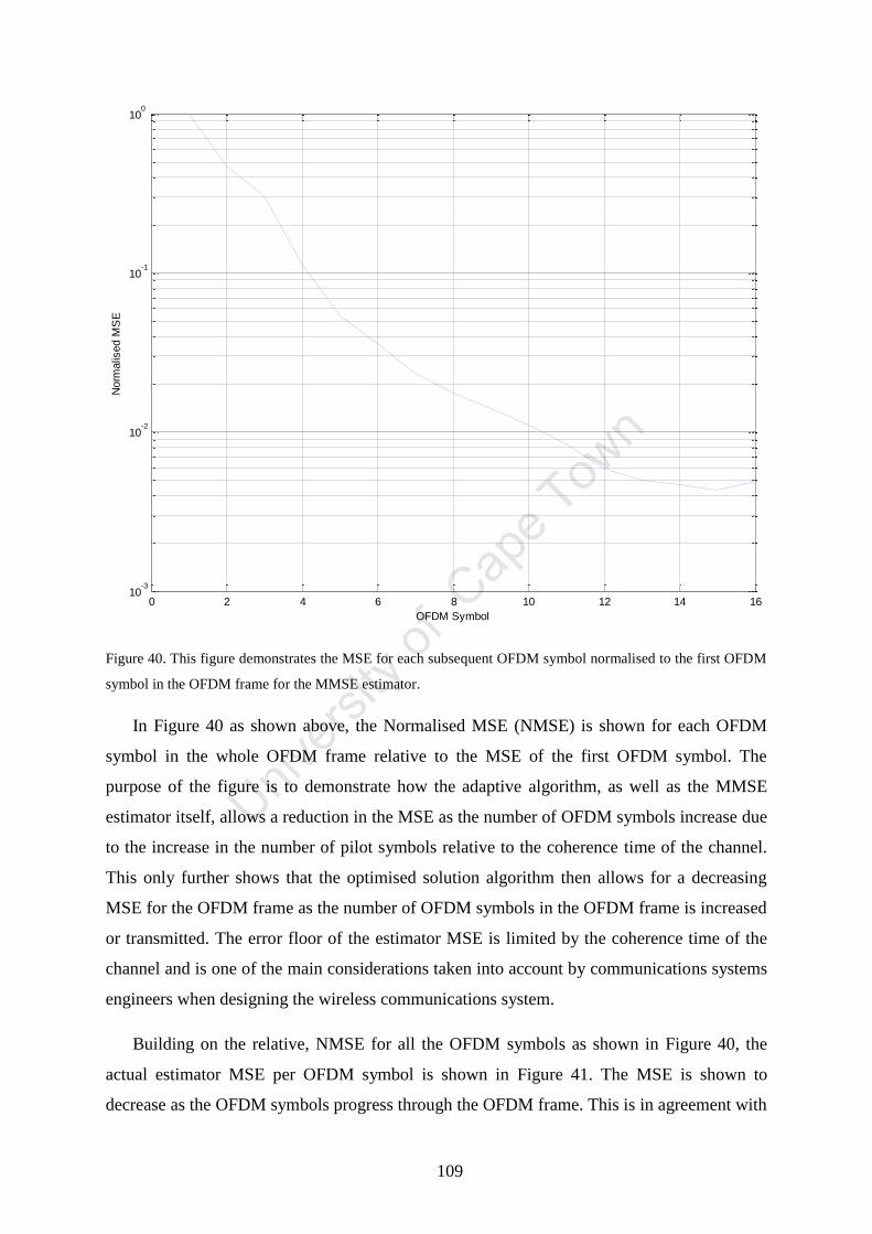
109

Figure 40. This figure demonstrates the MSE for each subsequent OFDM symbol normalised to the first OFDM

symbol in the OFDM frame for the MMSE estimator.

In Figure 40 as shown above, the Normalised MSE (NMSE) is shown for each OFDM

symbol in the whole OFDM frame relative to the MSE of the first OFDM symbol. The

purpose of the figure is to demonstrate how the adaptive algorithm, as well as the MMSE

estimator itself, allows a reduction in the MSE as the number of OFDM symbols increase due

to the increase in the number of pilot symbols relative to the coherence time of the channel.

This only further shows that the optimised solution algorithm then allows for a decreasing

MSE for the OFDM frame as the number of OFDM symbols in the OFDM frame is increased

or transmitted. The error floor of the estimator MSE is limited by the coherence time of the

channel and is one of the main considerations taken into account by communications systems

engineers when designing the wireless communications system.

Building on the relative, NMSE for all the OFDM symbols as shown in Figure 40, the

actual estimator MSE per OFDM symbol is shown in Figure 41. The MSE is shown to

decrease as the OFDM symbols progress through the OFDM frame. This is in agreement with

0 2 4 6 8 10 12 14 1610

-3

10-2

10-1

100

OFDM Symbol

Norm

alis

ed M

SE

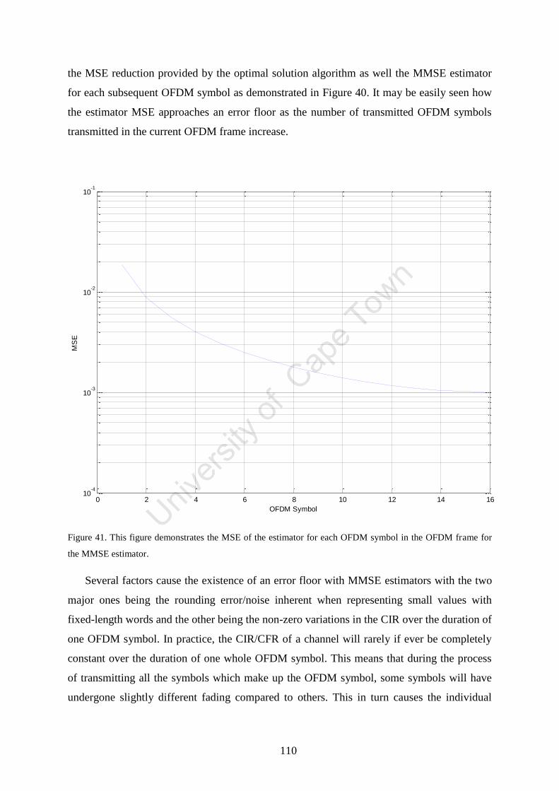
110

the MSE reduction provided by the optimal solution algorithm as well the MMSE estimator

for each subsequent OFDM symbol as demonstrated in Figure 40. It may be easily seen how

the estimator MSE approaches an error floor as the number of transmitted OFDM symbols

transmitted in the current OFDM frame increase.

Figure 41. This figure demonstrates the MSE of the estimator for each OFDM symbol in the OFDM frame for

the MMSE estimator.

Several factors cause the existence of an error floor with MMSE estimators with the two

major ones being the rounding error/noise inherent when representing small values with

fixed-length words and the other being the non-zero variations in the CIR over the duration of

one OFDM symbol. In practice, the CIR/CFR of a channel will rarely if ever be completely

constant over the duration of one whole OFDM symbol. This means that during the process

of transmitting all the symbols which make up the OFDM symbol, some symbols will have

undergone slightly different fading compared to others. This in turn causes the individual

0 2 4 6 8 10 12 14 1610

-4

10-3

10-2

10-1

OFDM Symbol

MS

E

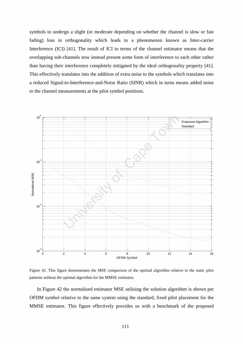
111

symbols to undergo a slight (or moderate depending on whether the channel is slow or fast

fading) loss in orthogonality which leads to a phenomenon known as Inter-carrier

Interference (ICI) [41]. The result of ICI in terms of the channel estimator means that the

overlapping sub-channels now instead present some form of interference to each other rather

than having their interference completely mitigated by the ideal orthogonality property [41].

This effectively translates into the addition of extra noise to the symbols which translates into

a reduced Signal-to-Interference-and-Noise Ratio (SINR) which in turns means added noise

to the channel measurements at the pilot symbol positions.

Figure 42. This figure demonstrates the MSE comparison of the optimal algorithm relative to the static pilot

patterns without the optimal algorithm for the MMSE estimator.

In Figure 42 the normalised estimator MSE utilising the solution algorithm is shown per

OFDM symbol relative to the same system using the standard, fixed pilot placement for the

MMSE estimator. This figure effectively provides us with a benchmark of the proposed

0 2 4 6 8 10 12 14 1610

-3

10-2

10-1

100

OFDM Symbol

Norm

alis

ed M

SE

Proposed Algorithm

Standard

112

solution compared to the current principle of having static pilot patterns. It may be seen how

the instantaneous NMSE per OFDM symbol is consistently lower when using the dynamic

pilot pattern (in other words, the proposed solution algorithm demonstrated in this document)

by a factor of about 10 compared to the traditional, static pilot pattern.

The finding above effectively allows us to conclude that a significant improvement in

estimator MSE may be had when utilising the proposed solution algorithms to solve the

contradictive problem addressed in this research compared to rather ignoring the issue and

utilising just a static pilot pattern and optimal power loading to maintain interference levels to

a desired threshold. It should be noted that the graph above, like most other MSE-based

comparisons in document presents the instantaneous MSE for each OFDM symbol which is

then plotted as the transmission of the OFDM frame progresses with the transmission of each

OFDM symbol. The overall MSE of the OFDM frame would therefore be the mean of each

of the instantaneous MSEs for all of the OFDM symbols in the OFDM frame. However, due

to the visibly consistent difference in NMSE when comparing the static pilot pattern to the

optimal solution algorithm, it may be concluded that the average MSE over the OFDM frame

will be about 10 dB lower when utilising the optimal solution algorithm.

The demonstrated MSE improvement shown in Figure 42 however does come at some

form of cost. Since the static pilot pattern does not have the addition of two pilot symbols

(one on either side of the PU transmission), there are two more data symbols when utilising

the static pilot pattern than compared to when using the solution algorithm derived in this

document. In the strictest sense, this means that the communications device may load data

symbols onto these and therefore provide some increase in transmission capacity. Due to the

proximity of these symbols to the PU transmission however, when utilising the optimal

power loading algorithm as described in [19] it means that the amount of power loaded to

these symbols will be significantly lower than compared to symbols placed a number of sub-

channels further away. As such, Adaptive Coding and Modulation (ACM) algorithms will

tend to place very small constellation sizes on those symbols due to their low SNR and

consequently result in an almost negligible gain in transmission capacity when compared

with the increase in estimator accuracy (reduction in MSE) when using the given solution

algorithms.

On a very important note, figures were not included showing the NMSE or MSE values

for each OFDM symbol for the LS estimator. This is due to the fact that both the MSE and

113

the NMSE remain constant for the LS estimator over a statistically significant sample of runs

and factoring out minor variations caused by measurement noise. This may be mainly

attributed to the static nature of the error function for the LS estimator which does not have

the kind of 'movement' or shifting as noticed in the case of the MMSE estimator because of

the presence of sinc functions in the cross- and auto-correlation functions. This directly

coincides with the findings of Figure 31 at the beginning of the section where the linear

increase in error function value through each progression through the OFDM frame by every

OFDM symbol translates into an approximately constant MSE for each of the OFDM

symbols in the OFDM frame.

It can be concluded therefore that unlike the MMSE estimator, the LS estimator does not

naturally converge to a lower estimator MSE with each transmitted OFDM symbol but is

rather much more dependent on the channel characteristics, the channel frequency response

specifically for each instantaneous OFDM symbol. This can therefore be interpreted as a

much higher independence for the current OFDM symbol from previous OFDM symbols and

as such it would make good practical sense to always employ some form of windowing for

the optimal solution algorithm when using the LS estimator since the marginal gains which

could be achieved by not windowing, and hence using the optimal algorithm, would not

justify the exponentially increased computational expense.

It is important to note that the provided optimal solutions solve the contradiction of power

loading and pilot patterns while also effectively reducing the estimator MSE when used by

the MMSE estimator for the case when a Single Input, Single Output (SISO) system is used.

This situation however does not necessarily apply to systems which use multiple antennae

(MIMO systems). This means that future research work could focus on investigating the

power loading and pilot pattern algorithms for the MIMO scenario as well as how the

identified contradiction changes in that situation. This would possibly lead to a different

solution to the identified problem which could possibly be adapted to be used in the general-

case scenario for any number of transmit and receive antennae. This also means that the

estimator MSE metric would have different results when simulating the MIMO-based

solution due to the different schemes available in exploiting the transmit and receive diversity

resulting in different possible simulation results when comparing the results on the estimator

MSE. In fact, this would also require different solutions due to the different MIMO

algorithms and schemes resulting in completely different modulator and demodulator

schemes and parameters.

114

5.2.3. Sub-optimal solutions

As MIMO is applied, the algorithm may be iterated over the pilot common pilot symbol

locations due to the time-frequency grid being independent of which antenna is used. This

however does not mean that the addition of MIMO may be considered as trivial and

transparent due to the requirements for precise timing and synchronization requiring adaption

of pilot patterns in practical implementations, as demonstrated in [54]. Work would therefore

need to be done as to resolve the situation if there is a contradiction between the two

algorithms. The computational complexity would, at the worst-case be multiplied again by

the number of transmitting and receiving antennas. This is due to the fact that each

combination of transmit-receive antenna pairs would experience different channel conditions

but it should be noted that this phenomenon already affects current pilot pattern algorithms as

well as demodulation since they also depend on channel state information to be executed.

This, while computationally inefficient, would however also be the trivial case to applying

the algorithm to a MIMO situation so that the sub-channels of interest (the search space) are

investigated transmit-receive pair so that the different CSI is accounted for each pair and an

aggregate decision is made as to where to place the pilot symbols.

The sub-optimal solution algorithm simulation results are demonstrated in this section,

with the results being grouped by the types of estimators being simulated. The results for the

sub-optimal algorithm in the LS estimator context are demonstrated in Section 5.2.3.1 and the

likewise results but for the MMSE estimator context are shown in Section 5.2.3.2.

5.2.3.1. LS estimator results

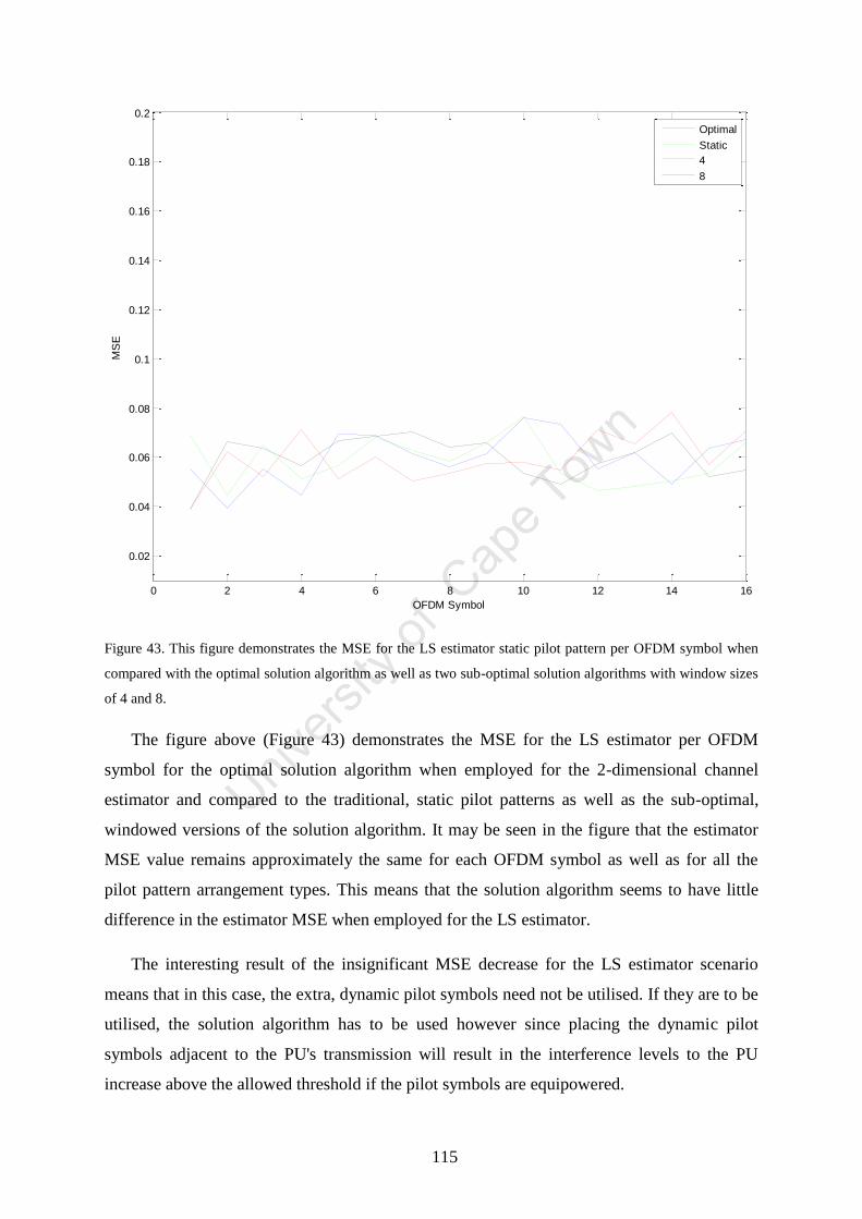
115

Figure 43. This figure demonstrates the MSE for the LS estimator static pilot pattern per OFDM symbol when

compared with the optimal solution algorithm as well as two sub-optimal solution algorithms with window sizes

of 4 and 8.

The figure above (Figure 43) demonstrates the MSE for the LS estimator per OFDM

symbol for the optimal solution algorithm when employed for the 2-dimensional channel

estimator and compared to the traditional, static pilot patterns as well as the sub-optimal,

windowed versions of the solution algorithm. It may be seen in the figure that the estimator

MSE value remains approximately the same for each OFDM symbol as well as for all the

pilot pattern arrangement types. This means that the solution algorithm seems to have little

difference in the estimator MSE when employed for the LS estimator.

The interesting result of the insignificant MSE decrease for the LS estimator scenario

means that in this case, the extra, dynamic pilot symbols need not be utilised. If they are to be

utilised, the solution algorithm has to be used however since placing the dynamic pilot

symbols adjacent to the PU's transmission will result in the interference levels to the PU

increase above the allowed threshold if the pilot symbols are equipowered.

0 2 4 6 8 10 12 14 16

0.02

0.04

0.06

0.08

0.1

0.12

0.14

0.16

0.18

0.2

OFDM Symbol

MS

E

Optimal

Static

4

8

116

When looking at the reason for the negligible MSE improvement of the optimal solution

algorithm compared to the traditional, static pilot pattern, we can determine the cause to be

the really low power loading levels for sub-channels near the PU. This means that the SNR

for those same sub-channels will be extremely low compared to the SNR for symbols farther

away. This results in higher measurement noise and as such when pilots are placed in that

region, the noise translates directly to added measurement noise for the LS estimator. In the

case of the LS estimator and its heuristic function, this results in the pilot symbol error

component of the equation increasing significantly.

The pilot symbol noise in the LS estimator heuristic function however is balanced out by

the interpolation error component when comparing the optimal and static pilot placement

algorithms/patterns. The loss of the two pilot symbols has a significantly negative effect on

the interpolation error term in the sense that there are now two extra distances between two

pairs of pilot symbols which need to be interpolated without any measurements/samples on

the other end. In all technically, this means that the positions now either have to be

interpolated over the relatively huge distance that is the PU's transmission band or they have

to be extrapolated from the previous pilot symbol values. For simplicity, it was assumed that

the values would be extrapolated by equating them to the value of the previous OFDM

symbol.

The high measurement noise due to the low SNR conditions present in the sub-channels

nearby is also compounded by the inversion/zero-forcing property of the LS estimator where

the CFR is the multiplication of the received symbol by the inverse of the transmitted symbol.

As such, symbols transmitted at a low SNR, due to the power loading algorithm attempting to

minimize interference, will in fact multiply the noise in a good number of cases. This was the

case in the simulation result noted above and is the reason that the MMSE estimator is a

preferred alternative to the LS estimator when complexity and computational time are not of

great concern and especially in situations where the channel estimator operates in low SNR

conditions.

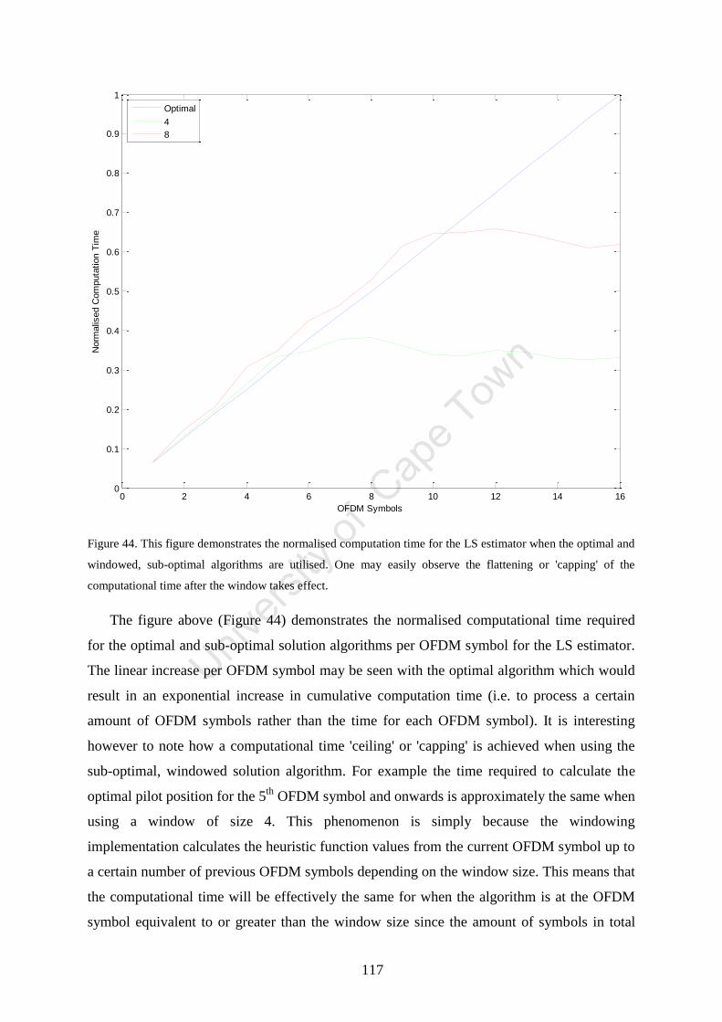
117

Figure 44. This figure demonstrates the normalised computation time for the LS estimator when the optimal and

windowed, sub-optimal algorithms are utilised. One may easily observe the flattening or 'capping' of the

computational time after the window takes effect.

The figure above (Figure 44) demonstrates the normalised computational time required

for the optimal and sub-optimal solution algorithms per OFDM symbol for the LS estimator.

The linear increase per OFDM symbol may be seen with the optimal algorithm which would

result in an exponential increase in cumulative computation time (i.e. to process a certain

amount of OFDM symbols rather than the time for each OFDM symbol). It is interesting

however to note how a computational time 'ceiling' or 'capping' is achieved when using the

sub-optimal, windowed solution algorithm. For example the time required to calculate the

optimal pilot position for the 5th

OFDM symbol and onwards is approximately the same when

using a window of size 4. This phenomenon is simply because the windowing

implementation calculates the heuristic function values from the current OFDM symbol up to

a certain number of previous OFDM symbols depending on the window size. This means that

the computational time will be effectively the same for when the algorithm is at the OFDM

symbol equivalent to or greater than the window size since the amount of symbols in total

0 2 4 6 8 10 12 14 160

0.1

0.2

0.3

0.4

0.5

0.6

0.7

0.8

0.9

1

OFDM Symbols

Norm

alis

ed C

om

puta

tion T

ime

Optimal

4

8

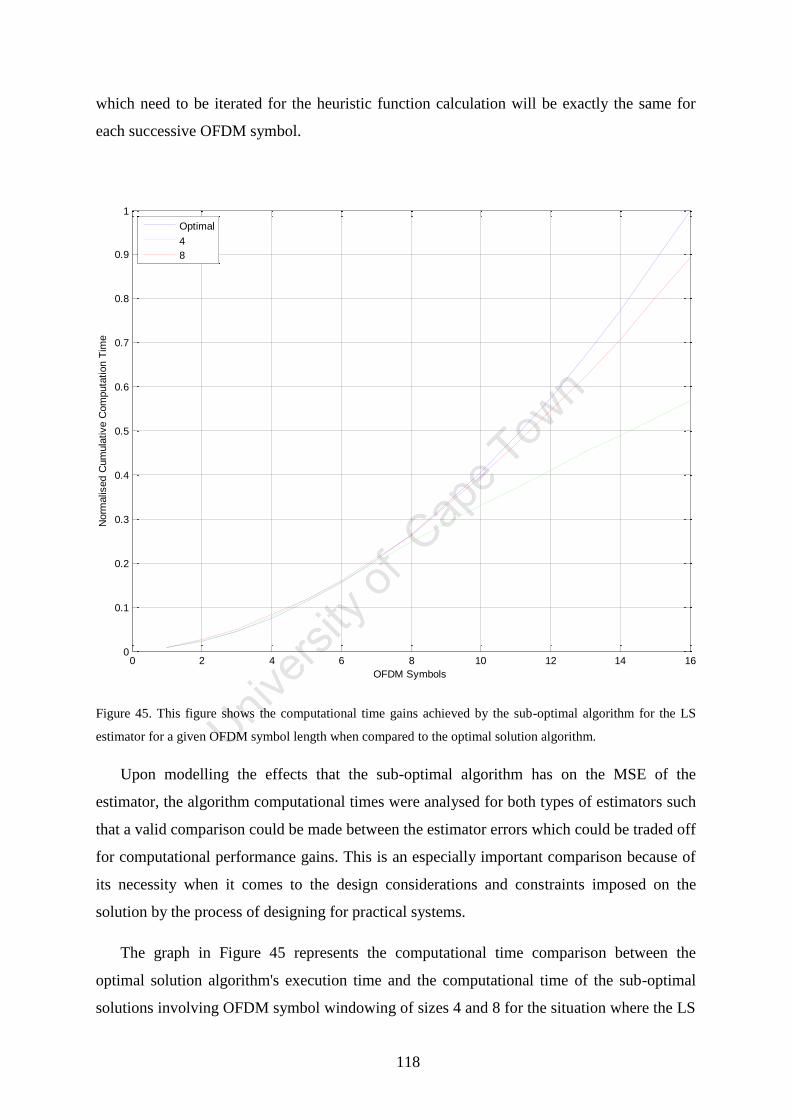
118

which need to be iterated for the heuristic function calculation will be exactly the same for

each successive OFDM symbol.

Figure 45. This figure shows the computational time gains achieved by the sub-optimal algorithm for the LS

estimator for a given OFDM symbol length when compared to the optimal solution algorithm.

Upon modelling the effects that the sub-optimal algorithm has on the MSE of the

estimator, the algorithm computational times were analysed for both types of estimators such

that a valid comparison could be made between the estimator errors which could be traded off

for computational performance gains. This is an especially important comparison because of

its necessity when it comes to the design considerations and constraints imposed on the

solution by the process of designing for practical systems.

The graph in Figure 45 represents the computational time comparison between the

optimal solution algorithm's execution time and the computational time of the sub-optimal

solutions involving OFDM symbol windowing of sizes 4 and 8 for the situation where the LS

0 2 4 6 8 10 12 14 160

0.1

0.2

0.3

0.4

0.5

0.6

0.7

0.8

0.9

1

OFDM Symbols

Norm

alis

ed C

um

ula

tive C

om

puta

tion T

ime

Optimal

4

8

119

estimator is employed. In the graph, it can be seen how the computational times follow an

exponential, albeit highly scaled down, increase corresponding to the increase in the number

of symbols (proportionally increasing with the number of OFDM symbols) in the OFDM

frame.

Interestingly enough, it may be observed in Figure 45 that the computational time for the

optimal and sub-optimal solution algorithms does not seem to have a big variance due to the

very small difference in symbols which need to be processed. This seems to be the case for

OFDM frames consisting of 7 or less OFDM symbols compared to the sub-optimal algorithm

with a window of 4. It would thus make perfect sense to consider the computational times

and utilise the optimal algorithm for very small length OFDM frames (such as 7 OFDM

symbols or less) and to use a sub-optimal, windowed solution for larger length OFDM frames

when using the LS estimator.

5.2.3.2. MMSE estimator results

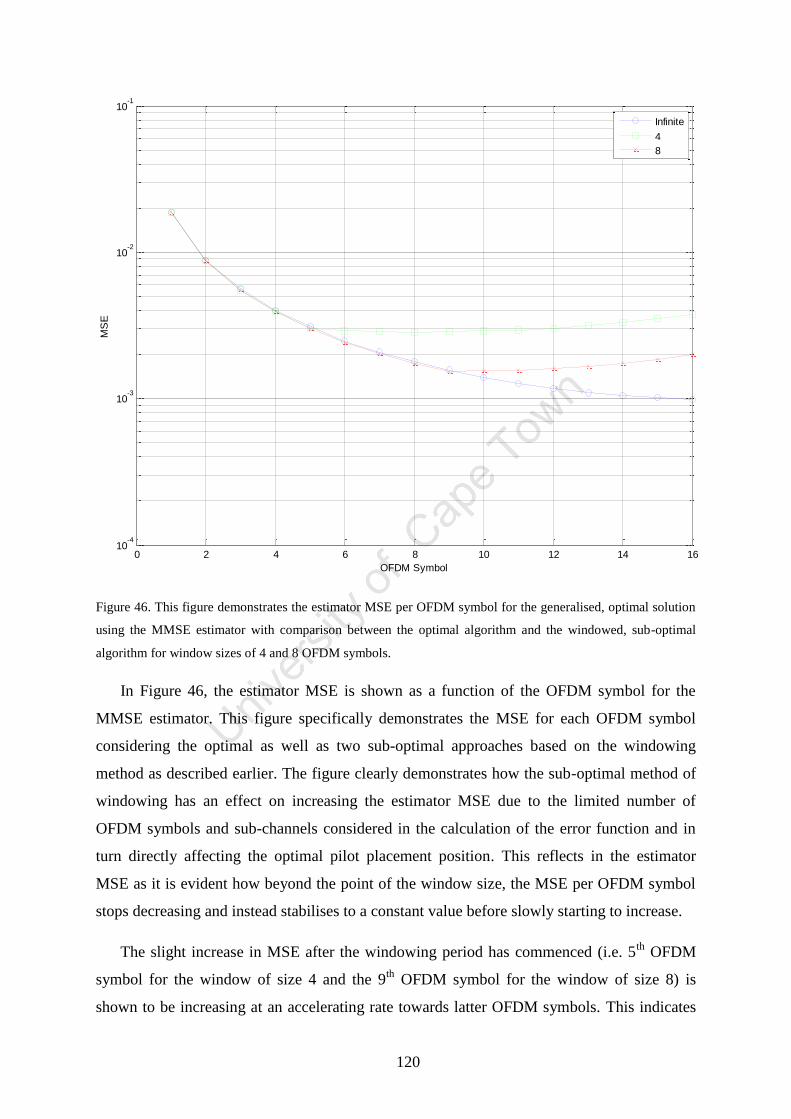
120

Figure 46. This figure demonstrates the estimator MSE per OFDM symbol for the generalised, optimal solution

using the MMSE estimator with comparison between the optimal algorithm and the windowed, sub-optimal

algorithm for window sizes of 4 and 8 OFDM symbols.

In Figure 46, the estimator MSE is shown as a function of the OFDM symbol for the

MMSE estimator. This figure specifically demonstrates the MSE for each OFDM symbol

considering the optimal as well as two sub-optimal approaches based on the windowing

method as described earlier. The figure clearly demonstrates how the sub-optimal method of

windowing has an effect on increasing the estimator MSE due to the limited number of

OFDM symbols and sub-channels considered in the calculation of the error function and in

turn directly affecting the optimal pilot placement position. This reflects in the estimator

MSE as it is evident how beyond the point of the window size, the MSE per OFDM symbol

stops decreasing and instead stabilises to a constant value before slowly starting to increase.

The slight increase in MSE after the windowing period has commenced (i.e. 5th

OFDM

symbol for the window of size 4 and the 9th

OFDM symbol for the window of size 8) is

shown to be increasing at an accelerating rate towards latter OFDM symbols. This indicates

0 2 4 6 8 10 12 14 1610

-4

10-3

10-2

10-1

OFDM Symbol

MS

E

Infinite

4

8

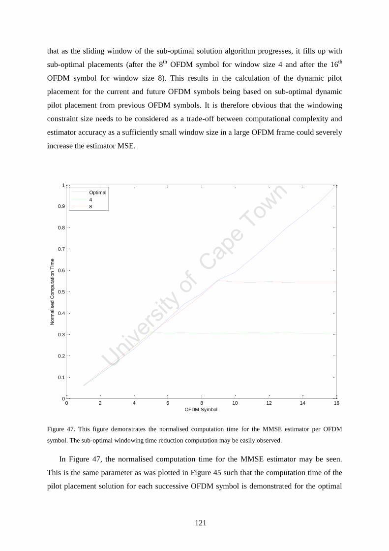
121

that as the sliding window of the sub-optimal solution algorithm progresses, it fills up with

sub-optimal placements (after the 8th

OFDM symbol for window size 4 and after the 16th

OFDM symbol for window size 8). This results in the calculation of the dynamic pilot

placement for the current and future OFDM symbols being based on sub-optimal dynamic

pilot placement from previous OFDM symbols. It is therefore obvious that the windowing

constraint size needs to be considered as a trade-off between computational complexity and

estimator accuracy as a sufficiently small window size in a large OFDM frame could severely

increase the estimator MSE.

Figure 47. This figure demonstrates the normalised computation time for the MMSE estimator per OFDM

symbol. The sub-optimal windowing time reduction computation may be easily observed.

In Figure 47, the normalised computation time for the MMSE estimator may be seen.

This is the same parameter as was plotted in Figure 45 such that the computation time of the

pilot placement solution for each successive OFDM symbol is demonstrated for the optimal

0 2 4 6 8 10 12 14 160

0.1

0.2

0.3

0.4

0.5

0.6

0.7

0.8

0.9

1

OFDM Symbol

Norm

alis

ed C

om

puta

tion T

ime

Optimal

4

8

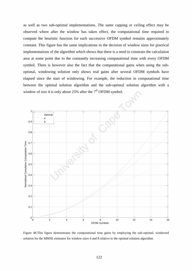
122

as well as two sub-optimal implementations. The same capping or ceiling effect may be

observed where after the window has taken effect, the computational time required to

compute the heuristic function for each successive OFDM symbol remains approximately

constant. This figure has the same implications in the decision of window sizes for practical

implementations of the algorithm which shows that there is a need to constrain the calculation

area at some point due to the constantly increasing computational time with every OFDM

symbol. There is however also the fact that the computational gains when using the sub-

optimal, windowing solution only shows real gains after several OFDM symbols have

elapsed since the start of windowing. For example, the reduction in computational time

between the optimal solution algorithm and the sub-optimal solution algorithm with a

window of size 4 is only about 25% after the 7th

OFDM symbol.

Figure 48.This figure demonstrates the computational time gains by employing the sub-optimal, windowed

solution for the MMSE estimator for window sizes 4 and 8 relative to the optimal solution algorithm.

0 2 4 6 8 10 12 14 160

0.1

0.2

0.3

0.4

0.5

0.6

0.7

0.8

0.9

1

OFDM Symbols

Norm

alis

ed C

um

ula

tive C

om

puta

tion T

ime

Optimal

4

8

123

In Figure 48, the cumulative computation time is demonstrated for the sub-optimal

algorithms employing window sizes of 4 and 8 relative to the computational time requirement

of the optimal algorithm for the MMSE estimator scenario. The same phenomenon may be

seen with Figure 48 as was noted in Figure 47 where the computational time for both the

optimal and sub-optimal algorithms is approximately the same in situations where the OFDM

frame is relatively small, i.e. 6 or less OFDM symbols in an OFDM frame. The algorithm

behaviour in terms of the computational time complexity and scalability for the MMSE

estimator may therefore be applied the same conclusion as that for the LS estimator, namely

that the algorithm presents interesting scenarios in terms of suitability.

As was shown with Figure 47, the MMSE estimator based algorithm may be efficiently

used optimally for OFDM frames with small sizes such as those consisting of 7 symbols or

less. For situations where the OFDM frame exceeds those sizes, the sub-optimal algorithms

could then be used. The windowing size would then purely depend on the practical situation

where the algorithms would be employed. For example, in situations where a rather large

OFDM frame size is employed, it would be more beneficial to use the sub-optimal,

windowed algorithm with a relatively smaller window size to ensure that computational time

does not become a major concern during the latter OFDM symbols comprising the OFDM

frame.

A very important aspect to the solution algorithm which needs to be stated is that the

design trade-off between optimal/sub-optimal window sizes and estimator error need not be

one based on a fixed, hard decision. Since the algorithm calculation methods for one OFDM

symbol are completely independent of the way in which they were executed in all previous

OFDM symbols and instead only rely on the time-frequency grid state for previous OFDM

symbols, the implementation of the solution algorithm could be done so that the solution

method dynamically switches between optimal and sub-optimal windowing sizes in different

situations. For example, when considering the MMSE estimator, the computational time

relative to the optimal algorithm is seen to be approximately the same for OFDM frames

which are 6 OFDM symbols in length or shorter. Significant divergence in relative

computational time between the optimal algorithm and the sub-optimal algorithm with a

window of 4 only occurs for OFDM frames which have a length greater than 7 OFDM

symbols.

124

When looking at the estimator MSE per OFDM symbol for the MMSE estimator as

shown in Figure 46 it may be seen that the constrained, sub-optimal solution for a window of

size 4 reaches its effective error floor after the 5th

OFDM symbol. This means that when

comparing this graph with the computational time as shown in Figure 48, an MMSE-based

system may be implemented by using the optimal solution algorithm (i.e. no window or

infinite length window) for the first 7 OFDM symbols and then switching to the sub-optimal

solution algorithm with a window size of 4. This can be generalised to a solution

implementation where a suitable trade-off is chosen for the design requirements such that the

instant reduction in estimator MSE provided by the optimal algorithm is combined with the

delayed appearance of significant computational time decrease provided by the sub-optimal,

windowed algorithm.

Another possible way which the algorithm could also be optimised for computational

time during the implementation stage is to use a state comparative approach to the use of the

algorithm. This approach involves the comparison of the current OFDM symbol for factors

which would influence the optimal pilot positioning relative to the previous OFDM symbol.

This approach has been proposed for the use of the optimal power loading algorithm in [19]

which involves the logic performing the calculation of the optimal power loading algorithm

to consider whether the system state has changed sufficiently (or if at all) to warrant a

recalculation of the optimisation constant ( ) so as to achieve the new optimal state. In the

case of the solution algorithm proposed, the factors influencing this would be the channel

frequency response, the appearance/disappearance of PUs (or more technically, the change in

the transmission power of PUs, including 0 dBm) or any change in the transmission

bandwidth of any of the PUs. Depending on the operating environment, the PU transmissions

could change from every OFDM symbol for a very busy environment such as 2.4 GHz to

never in heavily regulated spectrum such as terrestrial video broadcasting. Since OFDM

modulation based communications systems need to be designed such that the OFDM symbol

duration is much shorter than the channel coherence time ( so as to mitigate the ICI

phenomenon, in a large number of cases the channel will be slow fading. This means that the

channel would remain approximately constant for the duration of several OFDM symbols and

the optimal pilot positioning would only need to be recalculated at a certain, fixed interval

equal to or less than the channel coherence time in terms of number of OFDM symbols.

In all situations however, it may be seen that the computational time for both the optimal

and sub-optimal solution algorithms increase exponentially as the number of OFDM symbols

125

either indefinitely (optimal solution algorithm) or until the window size is reached (sub-

optimal solution algorithm). This means that for systems utilising large OFDM frame sizes,

future research could be investigated (outside the scope of this research problem statement)

aiming to address the computational complexity by providing an analytical solution by

approximating the transcendental functions used for the KKT optimisations. The further work

could also aim at reducing the computational complexity by utilising several techniques

which could efficiently reduce the computational time by either trading it off for memory

space or in fact centralising the computation to a powerful node with less practical

restrictions.

5.3. Comparison to Related Work

The simulation results demonstrated in this chapter were carefully evaluated so that they

may then be compared to relevant work solving the same or similar problem.

First and foremost, the related works described by [55], [51] or [52] attempt to address

the same basic problem of finding the optimal pilot positions for OFDM-based, non-

contiguous cognitive radio systems but the major factor missing from them is the identified

contradiction presented in this document where the interference between PUs and SUs need

be considered for optimal power loading of symbols. This means that in each case, the work

either considers just the pilot symbol positioning or it considers the power loading for the

pilot symbols as well but without considering the interference this would cause to adjacent

and nearby non-orthogonal users.

In [55] we can see that the authors propose a sub-optimal solution to the problem of

placing the pilot symbols in an NC-OFDM cognitive radio system as well as deriving the

optimal power loading for said pilot symbols. This solution however ignores interference

constraints from the SUs to the PUs as well as incoming interference from the PUs to the

SUs. This means that should the solution proposed by [55] be implemented in practise, the

same contradiction would still exist where the extra power afforded to pilot symbols causes

an increase to nearby PUs which could result in said OOB interference increase breaching

allowable or legal thresholds. The solution proposed in [55] also provides a sub-optimal

solution whereas the solution provided in this research is based on adapting the optimal pilot

126

placement algorithm to fit within the constraints of the optimal power loading algorithm in

the optimal way.

In [51], the same argument may be stated as well as it was for [55]. The proposed

solution in [51] again neglects to focus on interference constraints as well as incoming noise

to the pilot symbols whereas the work in [52] only addresses the pilot placement without

power loading of the pilot symbols themselves or interference caused to and by the pilot

symbols.

In terms of results, the work demonstrated in [51], [52] as well as [55] indicate an

approximate NMSE improvement factor of between 7-10 times, agreeing with the results

obtained from our estimation (a factor of about 9 times). As stated, the other research works

do not consider the out-of-band interference due to pilot placement as well as incoming

interference affecting the pilot symbol accuracy hence why the proposed algorithm in this

research has an NMSE on the lower (better) average of the related works surveyed.

127

6. Conclusions and Future Work

This section provides subsections which serve the conclusions as well as any

recommendations for future work which could expand on the proposed solutions in

conducted for the purposes of the research presented in this document.

The research conducted was focused on the principles of the engineering process. A

systematic approach to identifying and solving the problem was used such that a well-formed

engineering solution was obtained. The process initially focused on identifying the research

questions posed upon the commencement of the research work so that the problem could be

clearly defined. This meant that a quantitative description of the research problem could be

formulated so that a logical problem description with easily quantifiable solution goals would

be followed.

The next step required the identification of the requirements which a proposed solution

should have so as to be considered as successfully solving the identified research problem.

This meant that the research goals were quantified so that the proposed solutions to the

research problem could be assessed in terms of their viability as well as their practicality in

terms of implementation.

After the proposed solution requirements were quantified, the problem statement was

further analysed so that research was conducted into the existence of any already-devised

solutions or methods for solving the problem. The primary purpose of this exercise was to

determine whether there existed any solutions to the identified problem and if there were,

what their shortcomings were when compared with the proposed solution or design

requirements. This meant that the progression of the research would focus either on creating

new solutions for a previously unidentified problem (which was the case) or to improve upon

already-existing solutions so that they could be implemented practically in a more efficient

manner.

After the extensive research into the existence of solutions was conducted and it was

found that no solutions existed to the (newly) identified problem, the problem solution design

was formulated. This was done such that the proposed solution requirements were followed

and prioritised so that the design of the solution would be successful when compared to its

design requirements. The design was then thoroughly described and documented so that the

128

design process could be understood as well as the motivation and reasoning behind the

decisions made when designing the solution to the identified problem.

The next step involved the simulation and analysis of the proposed solutions to the

identified research problem. The developed solutions were simulated for different operating

parameters which were relevant to any practical implementations of the problem solution as

evidenced when identifying the solution requirements. This meant that the practical

feasibility of the proposed solutions could be investigated. This served the purpose of

allowing a quantitative analysis of the solution feasibility so that it could easily be seen how

the solution solves the identified problem in terms of measureable system performance

metrics. This also allowed the observation of if and how much the proposed solution

provided an improvement in terms of transmitter/receiver performance metrics when

compared with traditional methods which do not identify or resolve the researched problem.

Finally, after obtaining the simulation results as well as performing a quantitative analysis

on how the proposed solutions improve on current methods, the research questions originally

posed upon the commencement of research were answered. This was necessary so that an

objective outcome could be derived when evaluating the success of the proposed research

project in terms of the problems it addressed, the solutions it proposed and the viability and

practical feasibility of said solutions.

The steps above led in their own right to new conclusions during the research process

with the result of a large number of new and interesting results, the most obvious example

being that rarely, if ever, is the optimal pilot position adjacent to the primary user when

considering the optimal power loading algorithm.

The research which was conducted focused mainly on answer the 6 research questions

described in Section 1.7.1. These questions were regarded as a guideline for the progression

of the research and conclusions of them were formulated as follows.

Do any solutions exist for the identified contradiction? It was found that the identified

contradiction did indeed have an obtainable, optimal solution. The solutions were found to be

obtained by formulating the problem as a constrained, non-linear optimisation problem which

could be minimised so as to find the optimal dynamic pilot symbol placement which would

achieve the goal of minimising the estimator MSE while maintaining the power loading

profile to an optimal one. The solution was formulated in terms of functions for different

129

types of estimators (LS and MMSE) which could then be minimised so as to find the optimal

dynamic pilot symbol placement.

For which situations does the contradiction exist? The contradiction exists in all cases

where NC-OFDM is used as a modulation scheme and there is the possibility of interference

from PUs manifested as transmissions inside the SU band. As PU transmissions require the

disabling of sub-channels, this means that pilot symbols need to be adjusted as well as the

power loading to all sub-channels so as to avoid interference from both entities as well as to

maximise the transmission capacity given the (new) system conditions. As such, wherever

there are PU transmissions, it is highly likely that the estimator sampling (pilot symbols) will

be disturbed as well as the power loaded to nearby sub-channels. This would then require the

adaptation of the estimator to counteract the estimator accuracy losses caused by having to

disable several sub-channels of which 1 or more were likely to be pilot-symbol-bearing.

Are there any special cases where the contradiction does not exist or apply and how often

do they occur? While the contradiction theoretically exists in all such cases as described in

the previous question answered above, it will be significantly less pronounced in situations

where the PU transmission bandwidth is very small (narrowband) and/or the PU transmission

power is extremely low. Another such case would be on the other extreme where the PU

transmit power could be so extremely high that the optimal dynamic pilot placement is farther

away than the nearest static pilot symbol, meaning that the PU transmission negatively affects

nearby static pilot symbols as well. The former situation is of small concern as the dynamic

pilot symbols would naturally converge to be adjacent to the PU transmission bands.

However, in the latter scenario, the high PU transmission power and/or bandwidth would

result in very severe degradation in SU throughput and the high-power, wide-bandwidth

interference spectrum would mean that the static pilot pattern itself would need to be

reconsidered. This could be done by adapting the optimal solution algorithm proposed in this

document so as to calculate the pilot pattern as well. This would however be of great

computational complexity with current computing speeds.

How can the optimal solution be described mathematically? The optimal solution was

described mathematically through the use of fitness functions (error heuristics) which could

be set as a minimisation objective function so as to obtain the optimal pilot placement which

would satisfy the condition of minimising the channel estimator MSE/error while maintaining

optimal power loading levels such that interference from the SU to the PU was constrained

130

and kept to a fixed threshold as well as maximising the information throughput rates which

could be achieved by the SU.

How does the solution differ when between 1-dimensional and 2-dimensional pilot

patterns? The developed solution was initially completed for the situation where 1-

dimensional (frequency only) channel estimators were utilised. The relevant error/objective

functions were developed and tested. When investigating situations where 2-dimensional

(frequency and time) channel estimators are used, it was found that the same objective

functions that were used for the 1-dimensional estimator scenario could not be used for the 2-

dimensional estimator case. The 2-dimensional objective functions were therefore developed

so that the problem could be solved for situations where a 2-dimensional estimator is

employed. These objective functions were then generalised in the form of an algorithm so

that a general solution could be found for any scenario (1 or 2 dimensional) in which any type

of channel estimator is used. The solution in finding the optimal dynamic pilot symbol

placement could then be obtained by simply utilising the generalised solution algorithm

proposed in this document with the error heuristic (objective function) relevant to the

application context.

Are there any sub-optimal schemes or can any be developed? While the optimal

algorithm is indeed the most desirable solution to be used the computational time required in

order to obtain the optimal dynamic pilot symbol placement may need to be constrained in

practical applications where computing time and power are a constraint such as in embedded

devices. An investigation was therefore conducted into the computational time required for

practical scenarios such as those set out by the simulation parameters. It was found that the

bulk of computational time increase is when a 2-dimensional estimator was employed as this

required iterations through previous OFDM symbols in order to determine the optimal

dynamic pilot symbol position for the current OFDM symbol. This lead to the idea that the

algorithm should be windowed so that the computation of the optimal pilot symbol position

for the current OFDM symbol was limited as to how many previous OFDM symbols it would

consider and calculate in order to obtain the error function values for the candidate pilot

symbol positions.

It was found that when using windowing to reduce the algorithm computational time

requirement, the overall estimator error also increased for OFDM symbols after the start of

the first window exclusions as expected. This expense however resulted in a significant

131

computational time reduction for OFDM frame sizes which consisted of a significant number

of OFDM symbols. In fact, an interesting phenomenon was observed where the

computational time for the optimal and sub-optimal implementations of the solution

algorithm were approximately the same for smaller OFDM frame sizes. It was decided that

this property could be exploited such that the optimal solution algorithm is used for the first

few OFDM symbols and the sub-optimal, windowed algorithm is used for OFDM symbols

after which the computational time difference between the optimal and sub-optimal

algorithms would be significant.

6.1. Conclusions

From the beginning of the research process when preliminary literature reviews were

conducted, it was found that the most popular method of implementing cognitive radios was

through the use of NC-OFDM modulation. It was determined that this was so because of the

very high spectral efficiency achievable when using OFDM-based modulation schemes as

well as the ability to disable arbitrary sub-channel to avoid direct transmissions in primary

user bands. This ability also gave rise to another feature which allowed the cognitive radio

devices to transmit their modulated signals arbitrarily close to the PUs since only the sub-

channels which directly interfered with the PU were disabled and NC-OFDM allows there to

be no guard-bands between the different sub-channels, meaning that there is no spectral gap

between the SU and the PU transmissions. It was found that while this model provided

excellent spectrum utilisation efficiency, it also necessitated the re-working of several

important aspects which were needed for the optimal operation of contiguous OFDM

modulation to the non-contiguous case. The primary aspects which were investigated were

the power loading and the pilot pattern aspects.

It was found that the power loading algorithms needed to be adapted so that interference

between the SU and the PU needed to be considered as well due to the close proximity

between them when operating in an NC-OFDM cognitive radio environment. The result of

this was an optimal power loading algorithm described by [19]. This optimal power loading

algorithm was based on the water-filling algorithm which is optimal in the contiguous OFDM

sense. The NC-OFDM optimal power loading algorithm however also provides an added

control of an interference threshold which the SU needs to observe such that the cognitive

radio device is invisible and does not interfere with the licensed spectrum users. Once the

132

interference observations and constraints were implemented into the algorithm, the resulting

effect of this was that the power loaded to sub-channels was decreased as the distance

between them and the PU also decreased. This meant that sub-channels nearby to the PU

would have very little power loaded to them so as to keep interference levels low due to the

spectral properties of non-ideal pulse-shaping filter roll-off.

The other area which was also investigated for the purposes of the research is that of

optimal pilot patterns. As channel estimation and equalisation is an important aspect in the

optimal operation of OFDM systems, the research conducted into the optimal pilot patterns

was also deemed as highly relevant. The traditional forms of pilot pattern arrangement were

found to be based on static pilot patterns where the pilot symbols would be spaced at a fixed

interval distance in the OFDM frame. However, with the introduction of NC-OFDM, this

would result in some pilot symbols being disabled due to the requirement of having to disable

sub-channels which overlap with the PU transmissions. This condition meant that the

suitability of the static pilot patterns was not directly transferrable to the NC-OFDM case as a

large amount of channel sampling (pilot symbols) would be lost depending on the PU

bandwidths and the number of PUs. It was then found that an optimal solution did exist in

maintaining the estimator error (MSE) as low as possible in the NC-OFDM scenario. This

solution was provided by [24]. It was found that in this proposed, optimal solution the pilot

pattern needs to be dynamic in the sense that the symbols adjacent to the PU transmissions

need to be converted to pilot symbols so that the increase in estimator error caused by losing

the pilot symbols which would have been in the PU transmission is mitigated as much as

possible.

A contradiction was then identified where the optimal pilot pattern for NC-OFDM CR

devices dictates that the symbols adjacent to the PU transmissions be converted to pilot

symbols but the optimal power loading for NC-OFDM CRs dictates that the power of sub-

channels close to the PU be drastically reduced to maximise transmission capacity as well as

keep interference to the PU under a specified threshold. This resulted in a contradiction

where the new, dynamic pilot symbols would be placed in the worst possible conditions

(location) in an attempt to reduce estimator error. It was therefore decided that this problem

would be researched and an optimal solution would need to be found such that in practical

scenarios, where both optimal power loading and optimal pilot patterns need to be employed,

there would be an optimal solution so that both aspects could co-exist in an NC-OFDM

environment.

133

It was decided that before developing the solution, a list of requirements which the

solution would need to meet had to be resolved. These requirements mainly involved the

consideration of a practical implementation and feasibility of the solution which would be

proposed such that it is not only a theoretical solution but would also be practically

implementable as its whole purpose and existence was based on the solution of a practical,

implementation-level problem. These solution requirements are described in Section 1.7.2.

They include the development of a generalised solution which could be easily modified for

different possible application scenarios, the consideration of the most commonly used types

of channel estimators (LS and MMSE), the consideration of the two different types of pilot

patterns (1-dimensional and 2-dimensional) and the consideration of the computational time

required to compute the optimal, proposed solution.

Before developing the solution with the proposed requirements, an investigation was

done into whether any current solutions already existed and if they did what of the proposed

solution requirements they covered and which ones they did not. An extensive search was

conducted during the commencement of the research for any similar work which could

address the problem. There was however no such work found. Much work had been focused

on either the pilot pattern/channel estimation aspects of NC-OFDM CR systems as well as the

power loading aspects but no work was found which seemed to identify the problem and

contradiction originally identified in this document. It was deemed therefore that the work

which would be conducted for the purposes of this degree would lead to a novel solution to a

new problem were it to be developed.

Throughout the duration of the degree, a continuous search was also conducted for the

emergence of any similar research addressing the identified problem. There was however

none found. This also applied to the multitude of conferences attended by the student where

many fruitful discussions were held about the topic at hand as well as the invaluable feedback

received from fellow researchers in the field attending the conference and presentations of the

several papers presented. This further reinforced the opinion that the identified problem was

an original one with no known, published focus on it prior to this research. Trivially, this also

meant that the solution to the unique and unseen problem would also be unique and novel in

its own right.

The solution was then developed to coincide with the design requirements set out at the

commencement of the research project. Initially, the problem was analysed with the view of

134

the most simplistic case, namely the situation where a least squares, 1-dimensional channel

estimator is used. This allowed the preliminary results and feasibility of the research project

to be roughly gauged as it was to determine whether the hypothesis of the existence of an

optimal pilot symbol location not equivalent to the adjacent one proposed by the optimal pilot

pattern was correct from a rough observation.

The 1-dimensional solution was then extended to the MMSE estimator since it was the

next step in terms of the difficulty of the solution development. The MMSE estimator

required significantly more effort with respect to the design and development of the optimal

solution to the identified problem. It should be noted however that when developing the

solution, an algebraic solution was initially attempted through the use of the KKT conditions.

This however led to really complex objective functions and constraints which were

comprised of transcendental functions, most of which were trigonometric in nature. After

several weeks of attempted solutions to the problem of finding an analytical solution through

the use of the KKT conditions, it was found that the transcendental nature of the constraints

and the objective functions were simply too difficult to solve feasibly as was evidenced in

other research facing the same problems [37]. The detailed derivation of the KKT conditions

is described in Appendix A. The impractical difficulty in resolving the KKT conditions for

the formulated problem and obtaining an analytical solution was also compounded by the fact

that the actual search space for the solution, should it be implemented as a numerical search,

would be very limited and at worst case would be twice the pilot spacing interval (one for

each side of a PU transmission) multiplied by the number of PU transmissions in the SU

band. It was decided that the solution would therefore be implemented as a numerical search

algorithm.

Seeing as the situation for all cases (1-dimensional, 2-dimensional and MMSE or LS)

could ultimately be reduced as a numerical search of the optimal candidate pilot position

given some objective or heuristic function, it was decided that a generalised solution

algorithm was to be developed such that the algorithm need not be changed depending on the

situational context but rather only its parameters. A set of heuristic functions was therefore

developed to cater for the different application scenarios such that the same algorithm could

be used while only changing the heuristic function and the iteration area depending on the

number of dimensions used by the channel estimator.

135

The proposed generalised solution algorithm and its optimal heuristics functions were

then tested to determine their suitability as well as performance. The testing was done by

simulating a practical scenario and cognitive radio system which could be employed in future

implementations. The simulations were run to gather a statistically significant number of

samples and to account for noise for results for which it was necessary.

When analysing the results, it was found that the optimal pilot placement for most

situations was contrary to what was described by the optimal pilot pattern algorithm

described in [24] when the optimal power loading algorithm was considered. In most

practical situations, the optimal position for the new dynamic pilot symbols was actually a

number of sub-channels away from the PU transmission band due to the extreme interference

and noise conditions present near the PU bands as well as the resulting low SNR conditions

posed by the optimal power loading algorithm reacting to the bad noise and interference. The

optimal solution algorithm therefore provided different yet intuitive results when compared to

the optimal pilot pattern algorithm in [24] and [34] since the optimal pilot symbol positions

were not adjacent to the PU transmissions and were expected not to be due to the extremely

bad conditions for channel sampling and estimation present there.

The simulations used to evaluate and analyse the solution algorithm's suitability also

provided an interesting result in terms of the estimator accuracy improvement provided by

them. It was found that the estimator accuracy was increased by an average of 10 dB over

each OFDM symbol in the OFDM frame when comparing the optimal solution to a system

using a static pilot pattern with no adaptation when using the MMSE estimator. It was found

that in the case of the LS estimator however that for most cases the solution algorithm (be it

optimal or sub-optimal) did not provide any significant decreases in channel estimator MSE

compared to the traditional, static pilot pattern. This result does not invalidate the proposed

solution for the LS estimator however since the placement of pilot symbols nearby the PU

still needs to consider the optimal power loading algorithm such that interference to the PU

does not exceed the specified interference threshold. The solution algorithm would still be

necessary then to ensure that the placement of static pilot symbols is done in the optimal way

possible such that the estimator MSE is reduced to the lowest possible value while

conforming to the optimal power loading algorithm for CR NC-OFDM systems.

With respect to the LS channel estimator, it was found that for the used simulation

parameters, the channel estimator MSE did not achieve significant improvements. The

136

proposed solution algorithm did indeed provide the optimal pilot placement such that the

dynamic pilot symbols may be placed at a distance between the PU and the nearest static pilot

symbol so that the interference to the PU transmission band caused by the SU remains below

or equal to the specified design interference threshold ( ). As such, the requirement of the

solution was achieved for the LS estimator in that the optimal position for the dynamic pilot

symbols was found but it turned out that for the simulation parameters used, the dynamic

pilot symbols did not provide an improvement (decrease) in the estimator MSE. This was

principally attributed to the fact that the LS estimator in general is a lot more sensitive and

affected by noise than the MMSE estimator. In fact, the whole premise upon which the

MMSE estimator is based is to reduce the shortcomings of the LS estimator where the MSE

may drastically increase in conditions where a significant amount of noise is present.

Since the LS estimator obtains the estimated CFR by inversion of the transmitted pilot

symbols multiplied by the received pilot symbols, for situations where the pilot symbols are

in a low-SNR condition, this means that the noise will be significantly multiplied due to the

mathematical inversion of a relatively small number resulting in a relatively large number.

This was especially true for the simulation scenario that was used due to the optimal power

loading algorithm allocating significantly less power to the sub-channels nearer to the PU,

thus resulting in a much lower SNR for those same sub-channels. Since those sub-channels

were of interest in terms of placing the dynamic pilot symbol, the placement of the dynamic

pilot symbols would then have been in a low-SNR sub-channel, resulting in significantly high

amount of measurement noise for those specific pilot symbols. The solution algorithm then

balanced out the pilot symbol noise components and the interpolation error components of

the heuristic error function. While this did not have a significant impact in improving the

estimator MSE in the simulation scenario used, it may be hypothesised purely by knowing

the workings of the algorithm and heuristic functions that there will be an improvement in

situations where any a number of factors such as a larger static pilot symbol interval is used, a

lower PU bandwidth is present, a higher interference threshold for the PU is used (albeit

impractical due to licensing regulations being strict on interference between adjacent

channels belonging to different entities) and lower PU transmission power is present in the

system.

The suitability of the solution was then analysed specifically with respect to the

computational time requirement for both optimal and sub-optimal implementations. It was

found that the sub-optimal implementations provided a substantial decrease in the amount of

137

computation time required to compute the pilot positions for situations where the OFDM

frame consisted of a significantly large amount of OFDM symbols. An expected phenomenon

was observed where the use of windowing to provide a sub-optimal solution algorithm

resulting in the 'capping' or limiting of the computational time required for the algorithm with

each successive OFDM symbol after the window had been filled. This meant that the

computational time was effectively constrained for the windowed algorithm whereas the

optimal algorithm would have its computational time increase with every subsequent OFDM

symbol. This was deemed a necessary and imperative adaptation since for applications where

the amount of OFDM symbols in the OFDM frame are significantly large there would be a

situation where the computational time of the algorithm would be extremely taxing and

prohibitive. The windowing of the algorithm allowed this time to be reduced to a fixed one

(dependent on the window size) such that once the window had been filled, every subsequent

OFDM symbol would have approximately the same computational time as the previous one.

The advantage in computational speed provided by the sub-optimal algorithm also came

with a price however. The estimator MSE was significantly increased when using the sub-

optimal solution algorithm compared to the optimal solution algorithm. As the sub-optimal

algorithm provided an execution time ceiling it also provided an MSE floor when used for the

MMSE estimator. When using the optimal solution algorithm for the MMSE estimator, the

MSE was seen to decrease with each OFDM symbol, albeit with a slower rate as the number

of OFDM symbols increased. This was however not the same for the sub-optimal solution

algorithms since the windowing also provided an MSE floor which was achieved after the

window was filled. Like the computational time, this limit was also reached immediately

after the window was filled and therefore significantly increased the overall average MSE for

the OFDM frame. It is this trade-off that would need to be factored into a system design as

the smaller window sizes reached their limits quicker, meaning that the average

computational time for an OFDM frame would be much lower but the average estimator

MSE for the OFDM frame would also be higher.

In terms of difference between the optimal and sub-optimal solution algorithm

performance (estimator MSE) for the LS estimator, it was found that the difference was

marginal. This was attributed to the higher sensitivity of the LS estimator to noise and

therefore no significant change in estimator MSE per OFDM symbol could be seen as the

OFDM frame progressed. It is therefore logically practical to employ the sub-optimal

solution algorithm in practical scenarios when the channel and system parameters and

138

conditions match those used for the simulation parameters. This does not necessarily hold

true for all channel and system parameters due to the fact that the LS estimator's high noise

sensitivity translates to very 'dynamic' and easily variable results. It is therefore possible (and

likely) that in situations where the LS estimator has less measurement (pilot symbol) noise

the optimal algorithm would most likely provide an increase in estimator performance

(decrease in MSE) and would therefore result in different estimator MSEs per OFDM symbol

for optimal and sub-optimal implementations.

In general, it was found that the choice between optimal and sub-optimal

implementations of the solution algorithm would need to be made by the engineers designing

the practical implementation of the system. This decision may be made by using several

proposed optimisations such that either the fully-optimal algorithm is used (usually for

situations where small OFDM frame sizes and FFT sizes are to be used and computational

time and power consumption are not of priority, such as the proposed use in base-stations for

infrastructure-based cognitive radio systems) or a number of sub-optimal techniques. The

system designer would then decide on the best compromise of the estimator accuracy loss

(MSE increase) and computational speed. In all cases however, the solution algorithm

proposed in this research document would be needed should the designers wish to implement

the optimal power loading algorithm as well as the optimal pilot pattern algorithm in the

same NC-OFDM cognitive radio system.

Ultimately, the proposed solutions (both optimal and sub-optimal) were analysed to

determine whether they met their original design requirements as well as how they compared

to them. It was found that the derived solutions met and exceeded the proposed design

requirements set forth at the commencement of the research project. The solution to the

identified problem was successfully modelled and designed into a generalised algorithm with

a modular capability. This meant that the algorithm could be easily adapted for whatever

situation it needed to be utilised in with minimal modification. The algorithm could also be

used for both LS and MMSE estimators as well as proving easy to be adapted for less

common estimators such as the Maximum Likelihood (ML) estimator.

The algorithm also proved to significantly increase the performance of the channel

estimator when compared to traditional, static pilot patterns. The algorithm was shown to

decrease the estimator MSE by as much as 10 dB for the MMSE scenario and, while not

decreasing the MSE in the simulation scenario used for the LS channel estimator, did provide

139

the optimal pilot placement compromise as stipulated in the design requirement for both the

LS and MMSE channel estimators. Even for situations where the algorithm provides

marginal improvements in MSE it would still be deemed successful and necessary given that

if the optimal power loading algorithm and the optimal pilot pattern algorithms were

implemented without concern of each other, it would result in either interference levels to the

PU beyond the acceptable thresholds or significantly degraded estimator MSE due to the

large amounts of noise introduced into the CFR samples (the pilot symbols) due to the pilot

symbols being adjacent to the PU transmissions.

The conducted research work may also be analysed from the point of contributions

provided by the developed solutions to the described problem. From an initial point of view,

it may be seen that the research work first identifies and describes a contradictory problem

critical to the implementation of NC-OFDM cognitive radios where none such was found to

have been previously described.

Secondly, the research work provides proposed solutions for different channel estimator

scenarios to the identified, contradictory problem so that when the need arises to implement

an NC-OFDM cognitive radio using optimal pilot-pattern and power-loading algorithms, an

algorithm exists which may be used to replace both of these algorithms and provide an

optimal pilot-pattern with optimal power-loading so that no contradiction or degradation

exists between both.

Thirdly and finally, the research work derives and provides the heuristic functions used to

obtain the optimal solutions such that they may be used and implemented in any custom

solution algorithm deemed fitting.

While providing several important contributions for the successful implementation of

optimal pilot-pattern and power-loading algorithms in NC-OFDM cognitive radios, the

proposed solution algorithm also has several drawbacks, the main one being the

computational time. As the algorithm requires the iteration over all solution-candidate pilot

patterns, of which each entails over all current and previous symbols in the OFDM frame, the

computational complexity would fall into the O(n3) category. This is further compounded by

the fact that the heuristic functions are comprised of computationally intensive terms

involving trigonometric functions. This could therefore pose to be a big limitation on the

algorithm for cases where very large OFDM frames are used.

140

6.2. Future Work

This section describes ideas for future research work which could be conducted so as to

improve the proposed solutions to the identified problem. The future work concerned mainly

focuses on reducing the computational time required to obtain the solutions for different

scenarios, especially where large OFDM frame sizes are considered.

Section 6.2.1 describes possible future work on a series expansion of the problem

formulation. Due to the large number of transcendental functions present in the objective

functions, the analytical solution was deemed too difficult to solve through the use of KKT

conditions. The objective function could be approximated though using a series expansion.

This would allow the objective function to be simplified to a known form which could then

be solved to find the analytical solution to a sufficiently accurate approximation.

Section 6.2.2 describes the use of different pulse-shaping functions to model the PU and

SU transmissions and consequently their interference PSDs. The use of the rectangular pulse-

shaping functions in this research is not practically used due to their implementation

requirement necessitating non-causal implementations and therefore limiting them as being

ideal pulse-shaping filters. There are however a large number of practically usable pulse-

shaping functions which could be used to describe an even more accurate model of the

interference caused between the PU and the SU, allowing for even more accurate solutions to

the identified problem.

Section 6.2.3 proposes the extensions of the solution algorithms to the MIMO scenario.

Since many practical systems today employ MIMO to achieve better information transfer

rates without utilising a larger transmission bandwidth. It would be of great practical

importance to extend the solution to MIMO systems due to their widespread prevalence and

use in achieving higher data rates while utilising the same amount of bandwidth.

Section 6.2.4 deals with further optimisations to the generalised solution algorithm

proposed in this document. The section looks at possible practical implementations for

cognitive radio systems and how these could be exploited to achieve a lower computational

time for the solution algorithm. The concept of offloading the calculation of the optimal pilot

patterns is also investigated where the decision making could be moved to systems more

suitable and with much more relaxed computational time and power consumption constraints.

The section also examines some of the characteristics of the solution algorithm and proposes

141

ways in which it could be implemented such that the lowest possible estimator error is

achieved while keeping the computational time cost at an almost negligible difference.

6.2.1. Series expansion for analytic solution

As identified earlier, determining the analytic solution to the problem would prove useful

in allowing a detailed mathematical analysis. It is however very difficult to determine the

solution analytically and due to the fact that similar levels of computation will be necessary

even for the analytical solution when implemented in practise, the benefit of having an

analytical solution seems to be only in the theoretical analysis. The benefits however would

still serve well in determining better sub-optimal solutions which could provide the same

MSE for even lower computation times.

One possible way of determining an analytic solution is by approximating the KKT

conditions and formulation through the use of series expansions. Series expansions allow a

usually complicated mathematical function to be approximated by the summation of simpler

terms. The degree of accuracy of the expansion is usually dictated by the amount of terms (or

alternatively, the amount of summations) present in the series expansion.

One famous example of a series expansion is the Taylor series. The Taylor series may be

applied to functions which are infinitely differentiable, or more conveniently known as

smooth. This means that any functions which may be derived an infinite amount of times as

well as having all of these derivatives be continuous, may also be represented as a Taylor

series. Since the functions comprising the KKT conditions and those comprising the actual

objective function are primarily characterised by trigonometric, transcendental functions, this

criterion should be met by the optimisation problem.

If a successful Taylor expansion may then be obtained for the non-linear optimisation

problem and as such an analytical solution could be built around an approximation of a

sufficient degree and accuracy. This would then allow a better analysis of the problem

solution however at the expense of some accuracy due to the Taylor series approximation.

There also exist other series expansions possible for the trigonometric-based optimisation

and constraint functions, an example being Madhava series. An evaluation could be

performed determining their suitability and the best one could be chosen based on factors

such as accuracy, sufficient series length and computational cost.

142

6.2.2. Pulse-shaping functions

When formulating the optimal power loading algorithm as well as during the analysis of

the MMSE estimator, the general consensus is that both PU and SU transmitters utilise

rectangular pulse-shaping functions applied as windows to the transmitted symbols. The

purpose of this assumption is to achieve a level of simplicity when analysing a different

aspect of the system. While this approach is technically valid and is correct in theory, in

practise the rectangular pulse-shaping function is very rarely used due to its implementation

difficulty and large spectral roll-off characteristics.

The rectangular pulse-shaping function used to model the system could then be replaced

with a more practical one like the raised-cosine pulse-shaping function. This would mean that

the optimal power loading algorithm has to be essentially re-derived chiefly due to the

difference in the PDS of the PU-to-SU and SU-to-PU interference expressions. The MMSE

and LS estimator heuristics would however remain the same as they are independent of the

pulse-shaping function which is also an aspect applied in later stages of the transmission

chain and is therefore transparent to the channel estimator.

The change in pulse shaping function would therefore not affect the optimal or sub-

optimal solution algorithms but would change the results provided by them. Due to the

generally lower out-of-band interference caused by the raised-cosine pulse-shaping filters

compared to the rectangular ones, the interference would in general decrease in SU sub-

channels closer to the PU when compared with the equivalent rectangular pulse-shaping

function. This means that the error function values will tend to be lower and closer to the

PU's transmission band if the PU was modelled as using a raised-cosine pulse-shaping filter.

As such, the result of this would be that the solution algorithms would end up placing the

dynamic pilot symbols closer to the PU transmissions when using a raised-cosine filter than

when using a rectangular pulse-shaping filter, leading to decreased overall estimator MSE.

6.2.3. Extension to MIMO systems

Many communications systems nowadays exploit the easily achievable antenna diversity

available in mobile terminals. These systems are known as MIMO systems depending on the

amount of antennae used to transmit the signal and the amount of antennae used to receive

the signal. Through efficient precoding, MIMO systems may be effectively used to increase

143

effective information throughput of the system sometimes by several factors. It is therefore

no surprise that the utilisation of MIMO systems has become widely prevalent to coincide

with the higher data rates required with every new generation of digital communications

networks. In order to successfully implement MIMO systems however, optimal power

loading algorithms and optimal pilot pattern algorithms need to be adapted to include the

effects and changes necessary for the MIMO system.

The power loading algorithms needed for MIMO OFDM need to be adapted in order to

achieve the same desired optimal power loading allocation as is present in the SISO case. The

modified optimal power loading algorithm is based on the SISO optimal power loading

algorithm from [19]. The MIMO algorithm itself is described in [42] and may in summary be

seen to add an extra degree of freedom in terms of power loading (i.e. how much power to

which sub-channel on which antenna) from the traditional SISO scenario. As the power

loading algorithm does not affect the solution algorithm proposed by this document directly,

it should be trivial to extend the proposed solution algorithm without many modifications,

save for the adaptation of the algorithm, to a MIMO scenario. This therefore translates to a

generalisation of the algorithm to an even higher degree where any number of antennae could

be used by the PUs and the SUs.

The heuristic functions used to characterise the fitness of the proposed or candidate pilot

patterns by evaluating their MSE would also need adaptation in order to account for MIMO

systems. As the traditional, SISO based LS and MMSE estimators are evaluated in this

research, the heuristics functions would need to be updated to evaluate the estimator MSE

over the time-frequency grid with the added dimension of the antenna over which the

symbols are transmitted. Work on obtaining the optimal pilot pattern (or specifically spacing)

for MIMO dynamic spectrum access devices has been done and researched by [43] providing

a necessary background on the optimal pilot pattern for situations where pilot symbols are all

assigned the same amount of transmission power. As this research does not cover situations

where the pilot symbols would need to be assigned different amounts of power (as is shown

in the case of the research demonstrates in this document), there is a significant and yet

similar contradiction present in that the power loaded to symbols closer to PU transmissions

will need to be lower and will therefore always present situations where the location of the

pilot symbol will necessitate a different amount of power loaded to it so as to avoid breaching

interference thresholds required for the 'quiet' and legal operation of a cognitive radio device.

144

The proposed future work could then build on the principles of the work provided in this

document but with the difference being the change in optimal power loading and optimal

pilot pattern algorithms. These would then have the necessary constructs extracted from them

so as to allow a derivation of new heuristics functions which could be used to objectively

benchmark candidate pilot patterns so as to achieve the lowest estimator MSE possible while

maintaining interference levels from SUs to PUs at or below a desired threshold level. The

generalised solution algorithm would most likely not need to be adapted much other than to

add an extra iterator or element in searching through the extra added degree of freedom that is

the transmit and/or receive antennae. The algorithm itself however could be prone to added

optimisations simply due to the addition of the new degree of freedom allowing for a more

efficient approach to the already implemented solutions of both the 1-dimensional and 2-

dimensional algorithms.

6.2.4. Algorithm optimisations

Further research based on the work presented in this document would be very useful if

focusing on the aspect of computational time for the execution of the solution algorithm. The

algorithm proposed in this document at the time of writing could only be realistically

implemented on high-performance processors and would consume significant amounts of

power. Further research could be conducted into finding more efficient ways of computing

the heuristic function values of the candidate pilot symbol positions as the iterations through

other symbols to compute auto-correlations, cross-correlations and interpolation error bounds

consume a significant amount of time and power, especially when implemented in an OFDM

system with large OFDM symbol and OFDM frame sizes.

A common proposal of reducing the computational time in the MMSE scenario is to pre-

compute the auto-correlation matrix for the pilot symbols only when the pilot pattern itself

changes. While this would save a significant amount of time and power in situations where

the system operates in a band with low PU activity, this would not be the case for more

popular bands such as ISM 2.4 GHz where PUs' transmissions characteristics could change

with an average period of once every 4 OFDM symbols.

Another approach for reducing computational complexity in the device of implementation

would be to actually shift or offload the computational effort from the user terminal to the

base station in infrastructure-based cognitive radio systems. Since in a lot of cases the NC-

145

OFDM approach to CR implementation requires the use of an infrastructure architecture with

a controlling base station determining the allocation of bands to users as well as scheduling,

the task of pilot pattern designation and control would also be ceded to the base station due to

the need for co-ordinated channel estimation between all terminals. The optimal pilot pattern

would therefore only need to be calculated by the base station and not by the user terminals.

Since base stations are by definition fixed transceivers, there is a safe assumption that power

usage is not a significant constraint at all in the base station hardware and consequently the

available processing power of the base station will be significantly higher than that which is

available in the mobile terminals.

As was demonstrated in previous sections, the use of the windowing to create the sub-

optimal algorithms afforded significant decreases in the computational time required to

compute the solutions. This was however at the expense of estimator accuracy and had a

knock-on effect for latter OFDM symbols in the OFDM frame. This situation therefore posed

an interesting trade-off where essentially the computational time of the solution could be

traded-off for the accuracy of the desired solution and in general the estimator accuracy.

Further research could then focus on a further investigation of the error/computational

efficiency trade-off present in the sub-optimal algorithm. This would ideally lead to results

demonstrating the optimal window sizes for desired applications.

As proposed earlier as well, there is a trivial situation in terms of the accuracy/time trade-

off where the divergence in sub-optimal computational times relative to the optimal

computational time seems to significantly diverge only after a certain number of OFDM

symbols comprise the OFDM frame. It was thus proposed in Section 5.2.3 that the solution

algorithm's advantage of only depending on symbol layouts in previous OFDM symbols be

exploited and that the algorithms be switched from optimal to sub-optimal after a certain

number of OFDM symbols have been transmitted. This could be further developed into a

solution where the window sizes are dynamically adaptive and as the number of OFDM

symbols transmitted in the frame increase, so the algorithm window size decreases to

maintain the computational time below a desired threshold. The algorithm or rate for doing

this could be investigated in further research and promote better and more efficient solutions

in the future.

146

References

[1] J. Mitola III and G. Q. Maguire Jr., "Cognitive radio: making software radios more

personal," Personal Communications, IEEE, 1999, vol. 6, pp. 13-18.

[2] J. G. Proakis and M. Salehi, Communication Systems Engineering. Prentice Hall, 2002.

[3] Hyung G. Myung, Junsung Lim and David J. Goodman, "Single carrier FDMA for uplink

wireless transmission", Vehicular Technology Magazine, IEEE, 2006, vol. 1, pp. 30-38.

[4] A. M. Wyglinski, M. Nekovee and Y. T. Hou, Cognitive Radio Communications and

Networks: Principles and Practice. Academic Press, 2009.

[5] 3rd Generation Partnership Project (3GPP) Standard, "3GPP TS 36.201. LTE Physical

Layer," 2010.

[6] I. S. Board, "Part 11 : Wireless LAN Medium Access Control ( MAC ) and Physical

Layer ( PHY ) specifications High-speed Physical Layer in the 2.4 GHz Band," Control,

2003, vol. 1999.

[7] L. Vangelista, N. Benvenuto, S. Tomasin, C. Nokes, J. Stott, A. Filippi, M. Vlot, V.

Mignone and A. Morello, "Key technologies for next-generation terrestrial digital television

standard DVB-T2," Communications Magazine, IEEE, 2009, vol. 47, pp. 146-153.

[8] ITU-T, "G.992.1, Asymmetric digital subscriber line (ADSL) transceivers," 1999.

[9] D. L. Waring, "The asymmetrical digital subscriber line (ADSL): A new transport

technology for delivering wideband capabilities to the residence," in Global

Telecommunications Conference, 1991. GLOBECOM '91. 'Countdown to the New

Millennium. Featuring a Mini-Theme on: Personal Communications Services, 1991, pp.

1979-1986 vol.3.

[10] The Swedish Post and Telecom Authority (PTS), "The PTS spectrum auction in the 2.6

GHz band has been concluded.", 08/05/2008, vol. 2012.

[11] J. Silva and M. Dano, "700 MHz auction ends: Wireless heavyweights biggest players,

others surprise.", 21/03/2008, vol. 2012.

[12] I. F. Akyildiz, W. Lee, M. C. Vuran and S. Mohanty, "NeXt generation/dynamic

spectrum access/cognitive radio wireless networks: A survey," Computer Networks, 2006,

vol. 50, pp. 2127-2159.

[13] V. Valenta, Z. Fedra, R. Marsalek, G. Baudoin and M. Villegas, "Towards cognitive

radio networks: Spectrum utilization measurements in suburb environment," in Radio and

Wireless Symposium, 2009. RWS '09. IEEE, 2009, pp. 352-355.

[14] T. M. Taher, R. B. Bacchus, K. J. Zdunek and D. A. Roberson, "Long-term spectral

occupancy findings in chicago," in New Frontiers in Dynamic Spectrum Access Networks

(DySPAN), 2011 IEEE Symposium on, 2011, pp. 100-107.

147

[15] A. Leke and J. M. Cioffi, "A maximum rate loading algorithm for discrete multitone

modulation systems," in Global Telecommunications Conference, 1997. GLOBECOM '97.,

IEEE, 1997, vol. 3, pp. 1514-1518.

[16] N. Benvenuto and G. Cherubini, Algorithms for Communications Systems and their

Applications. J. Wiley, 2002.

[17] J. G. Proakis and M. Salehi, Digital Communications. McGraw-Hill, New York, 2008.

[18] Jiming Chen, Youxi Tang and Shaoqian Li, "Pilot power allocation for OFDM systems,"

in Vehicular Technology Conference, 2003. VTC 2003-Spring. the 57th IEEE Semiannual,

2003, vol. 2, pp. 1283-1287.

[19] G. Bansal, M. J. Hossain and V. K. Bhargava, "Optimal and Suboptimal Power

Allocation Schemes for OFDM-based Cognitive Radio Systems," Wireless Communications,

IEEE Transactions on, 2008, vol. 7, pp. 4710-4718.

[20] S. M. Kay, Fundamentals of Statistical Signal Processing: Estimation Theory. Upper

Saddle River, NJ, USA: Prentice-Hall, Inc, 1993.

[21] S. Takaoka and F. Adachi, "Pilot-assisted adaptive interpolation channel estimation for

OFDM signal reception," in Vehicular Technology Conference, 2004. VTC 2004-Spring.

2004 IEEE 59th, 2004, vol. 3, pp. 1777-1781.

[22] Meng-Han Hsieh and Che-Ho Wei, "Channel estimation for OFDM systems based on

comb-type pilot arrangement in frequency selective fading channels," Consumer Electronics,

IEEE Transactions on, 1998, vol. 44, pp. 217-225.

[23] Li Fu, Songlin Sun, Xiaojun Jing and Hai Huang, "Analysis of pilot patterns and channel

estimation for DVB-T2," in Network Infrastructure and Digital Content, 2010 2nd IEEE

International Conference on, 2010, pp. 609-613.

[24] I. Rashad, I. Budiarjo and H. Nikookar, "Efficient pilot pattern for OFDM-based

cognitive radio channel estimation - part 1," in Communications and Vehicular Technology in

the Benelux, 2007 14th IEEE Symposium on, 2007, pp. 1-5.

[25] Jinnan Liu, Shulan Feng and Haiguang Wang, "Comb-type pilot aided channel

estimation in non-contiguous OFDM systems for cognitive radio," in Wireless

Communications, Networking and Mobile Computing, 2009. WiCom '09. 5th International

Conference on, 2009, pp. 1-4.

[26] J. -. van de Beek, O. Edfors, M. Sandell, S. K. Wilson and P. O. Borjesson, "On channel

estimation in OFDM systems," in Vehicular Technology Conference, 1995 IEEE 45th, 1995,

vol.2, pp. 815-819 .

[27] O. Edfors, M. Sandell, J. -. van de Beek, S. K. Wilson and P. O. Borjesson, "OFDM

channel estimation by singular value decomposition," Communications, IEEE Transactions

on, 1998, vol. 46, pp. 931-939.

[28] M. Engels, Wireless OFDM Systems: How to make them Work? Norwell, MA, USA:

Kluwer Academic Publishers, 2002.

[29] S. Kaiser. Multi-carrier CDMA mobile radio systems - analysis and optimization of

detection, decoding, and channel estimation. 1998.

148

[30] T. Weiss, J. Hillenbrand, A. Krohn and F. K. Jondral, "Mutual interference in OFDM-

based spectrum pooling systems," in Vehicular Technology Conference, 2004. VTC 2004-

Spring. 2004 IEEE 59th, 2004, vol.4, pp. 1873-1877.

[31] Shichang Zhang, Jun Wang and Shaoqian Li, "A channel estimation method for NC-

OFDM systems in cognitive radio context," in Communication Systems, 2008. ICCS 2008.

11th IEEE Singapore International Conference on, 2008, pp. 208-212.

[32] S. D. Conte and C. de Boor, "Interpolation by polynomials," in Elementary Numerical

Analysis, an Algorithmic Approach, 3rd ed.Anonymous McGraw-Hill, 1980.

[33] H. Schulze and C. Lueders, Theory and Applications of Ofdm and Cdma: Wideband

Wireless Communications. John Wiley & Sons, 2006.

[34] I. Budiarjo, I. Rashad and H. Nikookar, "Efficient pilot pattern for OFDM-based

cognitive radio channel estimation - part 2," in Communications and Vehicular Technology in

the Benelux, 2007 14th IEEE Symposium on, 2007, pp. 1-5.

[35] H. W. Kuhn, "Nonlinear programming: a historical view," SIGMAP Bull., jun, 1982, pp.

6-18.

[36] R. T. Smith and R. B. Minton, Calculus: Early Transcendental Functions. McGraw-Hill

Higher Education, 2006.

[37] H. Wang, N. Agoulmine, M. Ma, Y. Li and X. Wang, "Network Lifetime Optimization

by KKT Optimality Conditions in Wireless Sensor Networks," Wireless Personal

Communications, 2009, vol. 49, pp. 179-196.

[38] T. H. Cormen, C. Stein, R. L. Rivest and C. E. Leiserson, Introduction to Algorithms.

McGraw-Hill Higher Education, 2001.

[39] V. Erceg, K. V. S. Hari, M. S. Smith and D. S. Baum, "Channel models for fixed

wireless applications," Contribution to IEEE 802.16.3, jul, 2001.

[40] V. Erceg, L. J. Greenstein, S. Y. Tjandra, S. R. Parkoff, A. Gupta, B. Kulic, A. A. Julius

and R. Bianchi, "An empirically based path loss model for wireless channels in suburban

environments," Selected Areas in Communications, IEEE Journal on, vol. 17, 1999, pp.

1205-1211.

[41] Yang-Seok Choi, P. J. Voltz and F. A. Cassara, "On channel estimation and detection for

multicarrier signals in fast and selective Rayleigh fading channels," Communications, IEEE

Transactions on, 2001, vol. 49, pp. 1375-1387.

[42] U. Phuyal, A. Punchihewa, V. K. Bhargava and C. Despins, "Power loading for

multicarrier cognitive radio with MIMO antennas," in Wireless Communications and

Networking Conference, 2009. WCNC 2009. IEEE, 2009, pp. 1-5.

[43] E. Golovins and N. Ventura, "Optimal pilot pattern design for dynamic spectrum access

MIMO multicarrier systems," in Personal, Indoor and Mobile Radio Communications, 2009

IEEE 20th International Symposium on, 2009, pp. 2030-2034.

[44] J. D. Parsons, The Mobile Radio Propagation Channel. John Wiley, 2000.

149

[45] S. Boyd and L. Vandenberghe, Convex Optimization. New York, NY, USA: Cambridge

University Press, 2004.

[46] Jun Cai, Xuemin Shen and J. W. Mark, "Robust channel estimation for OFDM wireless

communication systems - an H∞; approach," Wireless Communications, IEEE Transactions

on, 2004, vol. 3, pp. 2060-2071.

[47] Zhendong Luo and Dawei Huang, "Optimal and robust MMSE channel estimation for

MIMO-OFDM systems," in Personal, Indoor and Mobile Radio Communications, 2008.

PIMRC 2008. IEEE 19th International Symposium on, 2008, pp. 1-5.

[48] J. Stewart, Calculus: Early Transcendentals. Thomson/Brooks/Cole, 2003.

[49] J. F. Epperson, "On the Runge example," Am.Math.Monthly, 1987, vol. 94, pp. 329-341.

[50] R. Nilsson, O. Edfors, M. Sandell and P. O. Borjesson, "An analysis of two-dimensional

pilot-symbol assisted modulation for OFDM," in Personal Wireless Communications, 1997

IEEE International Conference on, 1997, pp. 71-74.

[51] E. Manasseh, S. Ohno and M. Nakamoto, "Pilot design for non-contiguous spectrum

usage in OFDM-based cognitive radio networks," in Signal Processing Conference

(EUSIPCO), 2012 Proceedings of the 20th European, 2012, pp. 465-469.

[52] Die Hu, Lianghua He and Xiaodong Wang, "An Efficient Pilot Design Method for

OFDM-Based Cognitive Radio Systems," Wireless Communications, IEEE Transactions on,

2011, vol. 10, pp. 1252-1259.

[53] A. Bhuvaneshwari and T. Sathyasavithri, "Comparative analysis of mobile radio path

loss models for suburban environment in southern india," in Emerging Trends in VLSI,

Embedded System, Nano Electronics and Telecommunication System (ICEVENT), 2013

International Conference on, 2013, pp. 1-5.

[54] Yuan Ouyang, Wei-Ju Chen and Sheng-Han Wu, "Channel estimation for MIMO-

OFDM systems using a novel STBC pilot pattern," in High Speed Intelligent Communication

Forum (HSIC), 2012 4th International, 2012, pp. 1-2.

[55] Youchang Zhang, Xiaodong Xu, Bin Chen and Xuchu Dai, "A suboptimal pilot design

for NC-OFDM systems," in Communication Technology (ICCT), 2010 12th IEEE

International Conference on, 2010, pp. 801-804.

[56] C. K. Tan, T. C. Chuah and S. W. Tan, "Fair subcarrier and power allocation for

multiuser orthogonal frequency-division multiple access cognitive radio networks using a

colonel blotto game," Communications, IET, 2011, vol. 5, pp. 1607-1618.

150

Appendices

This section contains any appendices required for deeper understanding into aspects

mentioned in any of the sections of this thesis. These aspects are especially useful should the

reader be interested in the mathematical or technical descriptions of the aspects which are

assumed in the sections above such that a deeper understanding may be developed as to why

and how the assumptions are made.

Appendix A introduces the reader to the detailed concepts and mathematical procedures

involved in obtaining the optimal condition of a constrained, non-linear optimisation problem

using the KKT conditions. The work shown in the appendix also demonstrates the attempted

use of the KKT conditions to find the analytical, optimal solution to the problem identified

and formulated in this research as well as a mathematical description of the reason this is

highly impractical and complex.

Appendix B demonstrates to the reader the detailed derivation and mathematical

differentiation between the LS and MMSE estimators. The appendix shows how the MMSE

estimator is indeed a modified version of the LS estimator with the added use of channel

statistics. It also demonstrates an analysis on the MMSE estimator in terms of analytical

descriptions as well as mathematical formulations and differences between the ideal and the

robust MMSE estimator.

Appendix C performs an analysis on the interpolators used for the equalisation of data

symbols when utilising the LS estimator. The appendix provides a detailed analysis of the

linear interpolator as well as providing a generalised version as well as error bound analysis

for higher-order interpolators. The section also provides an insight into the computational

effort required for the different orders of interpolators.

Appendix D provides in detail the different types of terrain models used in deriving the

channel models used during the simulation of the proposed solutions. The section provides a

detailed analysis into the different terrain models as well as how they affect the resultant

channel models which are built upon them. A description is also made into the way the

different terrain models ultimately affect the transmitted signals sent between the transmitter

and the receiver as well as their effects on the simulation in terms of practicality.

151

Appendix E provides an in-depth mathematical description of the two main types of

fading channel stochastic models, namely Rayleigh fading and Rician fading. The section

presents a mathematical description of the two different types of fading channels as well as

their statistical relationship. The appendix also provides the reader with some useful statistics

and properties of the two types of channels and their relevant probability functions. A graph

is also shown which demonstrates from a visual aspect the way the two different types of

fading channels behave.

152

Appendix A: KKT constraints of the optimisation problem

When performing non-linear optimisation, there are several methods which may be used

to analytically find the optimal solution to the formulated problem depending on the

properties of the formulated objective function. While there exist many classes of

optimisation problems, the one of relevance to the research which was conducted were non-

linear (convex specifically), constrained optimisation problems. The optimal solution to these

problems (for when it exists) may be found by utilising the KKT conditions.

The constrained, non-linear problem can be mathematically formulated as

For the constrained, non-linear optimisation problem, the candidate optimal solution

value may be defined as feasible if and only if (iff) the constraints specified in (A.1) (i.e.

and ) are met.

It is also essential to note that depending on the application requirements, the objective

function may need to be either minimized or maximized. In order to achieve the desired

result, the KKT conditions may be used in both applications with the difference being that the

objective function for maximization problems may simply be rewritten as a minimization

problem with a negated version of the objective function of the maximization problem.

In order to find all minima and maxima of the objective function, the derivative of the

function may be set to be zero and the function input may be evaluated. As such, any

optimal solution of any continuous optimisation problem will satisfy the following equation

where is by definition the optimal value of where the value of the objective function will

be a global minimum.

The concept of finding global optimal values by finding the point of the objective

function where its derivative will equate to zero may then be expanded when the problem is

constrained only by equality constraints. This is done through the use of Lagrange multipliers

which may be formulated through the Lagrange function defined as [45]

(A.1)

(A.2)

153

If we then use the principle of finding the points where the objective function derivative

is zero, we may obtain the Lagrange multipliers as

the vector differentiation may then be broken down by its dimensions as

and

The equations above present one of the KKT conditions for the existence of a global

minimum of the objective function, in other words, for the existence of an optimal solution to

the optimisation problem.

The formulation can then be extended to the situation where optimisation problem is

constrained by equalities as well as inequalities. This is done by introducing a multiplier

for each constraint such that

The introduction of the additional multiplier used for handling the added inequality

constraints then allows us to reformulate the Lagrange function to be defined as

The KKT conditions for the optimal solution of the constrained may then be formulated

as

∑

(A.3)

(A.4)

∑

(A.5)

(A.6)

(A.7)

∑

∑

(A.8)

154

The addition of the last condition is known as the complementary slackness condition

which is used to guarantee that the duality afforded by the Lagrange multipliers and is

limited in slackness.

The KKT conditions above provide the minima of the objective function defined by .

These points are also known as the stationary or KKT points. If one desires, the KKT points

may then be searched such that the global optimum is found. However, since the optimisation

problem we are focusing on is convex, it means that on the interval for which the function is

continuous ( ) there will only exist one local minimum which will also be a global minimum

[[45].

In order to attempt to find an analytic solution of the demonstrated problem, we may try

to find the global minimum of the LS and the MMSE error functions. The KKT conditions

may therefore be used to find these values.

For the LS estimator (1-dimensional), the KKT conditions may be obtained by using the

error function from equation (36) and the several constraints as follows

where the distance component has been replaced by the candidate pilot symbol position

variable since the distance to the nearest static pilot symbol may be obtained by its

Euclidean distance representation and the maximum of the second derivative of the CFR has

been replaced by a constant as the CFR is usually pre-computed and stored. The AWGN

component has also been represented as a constant due to the white noise assumption of

the AWGN noise meaning that the noise variance is approximately uniform for all

∑

∑

(A.9)

|

|

(A.10)

155

frequencies. As such, the second derivative of the CFR may also be stored in the same way

which results in very low computation time for obtaining the desired maximum.

From (A.10), the KKT conditions may then be formulated as

The representation of the constraint functions and the partial derivative of the objective

function may then be formulated into the following Lagrange function

thus, the equation provided above (A.12) as well as the constraints listed in (A.11) need to be

solved. This equation needs to be further expanded by considering the derivatives as follows

where

When substituting all the equations we see that we also need to obtain the derivative of

the optimal power loading equation with respect to the frequency component which in itself

needs to obtain the derivative of the interference component caused by the SU with respect to

the power loaded to it. Taking from (xx, power loading equation), we end up with

|

|

(A.11)

|

|

(A.12)

(A.13)

(

)

(A.14)

156

where Si is the sine integral denoted by

leaving us with the optimal power loading formulation as

This then leads to the complete Lagrange function as

As seen above, the formulation for the Lagrange function also needs to be stated for the

sub-functions involving their derivatives such as the formulation of

requiring the

derivation of

as well as the further use of

. The complexity of the Lagrange function

is therefore impractically high so that a successful analytical solution may be determined

through the use of the KKT constraints. While this problem is one from a practical point of

view, the more serious issue is that the Lagrange function would consist of a very large

number of trigonometric components as well as a sine integral. This therefore means that the

solution would be ambiguous should the trigonometric functions not cancel each other out

completely (which they won't due to the form of and

). As such, a global minimum

would most likely be non-existent and would actually appear as a series of local minima

should it get to the point where it could be formulated successfully.

(A.15)

∫

(A.16)

(

)

| |

(A.17)

|

|

(A.18)

157

For the formulation of the KKT conditions for the MMSE estimator, the same problem is

reached where the analytical solution is impractically difficult to obtain. In the same vein as

the attempted analytical solution for the LS estimator, the attempted analytical solution for

the MMSE estimator would also prove to have approximately the same computational

complexity as the numerical solution due to the relatively small search space of the solution

(i.e. the search space may at most be twice the static pilot symbol interval multiplied by the

number of PUs so that the optimal dynamic pilot symbol position may be calculated for each

side of every PU transmission in the SU transmission band). The calculation complexity for

the numerical computation as well as the analytical may also be practically halved due to the

relatively safe assumption that the optimal dynamic pilot symbol distance on one side of a PU

transmission will be approximately the same for the other side of the same PU transmission.

The obvious exception to this rule is when there is another PU transmission close to the

current one on only one side of the current PU transmission.

The attempted analytical solution for the MMSE estimator using KKT conditions may

then be formulated as

where

and

such that

with the conditions

(A.19)

(A.20)

{| | } (A.21)

( )

(A.22)

158

The formulation of the Lagrange function for the MMSE estimator scenario requires the

inclusion of the factor as the position of a static pilot symbol due to the auto-correlation

between different pilot symbols needing to be considered.

The complexity for the MMSE estimator scenario is even higher given the high number

of trigonometric functions present in the problem formulation. For example, simply deriving

the objective function in (A.22) presents us with the partial Lagrange function of

(A.23)

(

)

(

)

(A.24)

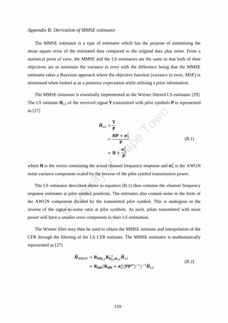
159

Appendix B: Derivation of MMSE estimator

The MMSE estimator is a type of estimator which has the purpose of minimising the

mean square error of the estimated data compared to the original data plus noise. From a

statistical point of view, the MMSE and the LS estimators are the same in that both of their

objectives are to minimize the variance in error with the difference being that the MMSE

estimator takes a Bayesian approach where the objective function (variance in error, MSE) is

minimised when looked at as a posterior expectation while utilising a prior information.

The MMSE estimator is essentially implemented as the Wiener filtered LS estimator [29].

The LS estimate of the received signal transmitted with pilot symbols is represented

as [27]

where is the vector containing the actual channel frequency response and is the AWGN

noise variance component scaled by the inverse of the pilot symbol transmission power.

The LS estimator described above in equation (B.1) then contains the channel frequency

response estimates at pilot symbol positions. The estimates also contain noise in the form of

the AWGN component divided by the transmitted pilot symbol. This is analogous to the

inverse of the signal-to-noise ratio at pilot symbols. As such, pilots transmitted with more

power will have a smaller error component in their LS estimation.

The Wiener filter may then be used to obtain the MMSE estimate and interpolation of the

CFR through the filtering of the LS CFR estimate. The MMSE estimator is mathematically

represented as [27]

(B.1)

(B.2)

160

where represents the channel auto-covariance (scaled auto-correlation) matrix,

represents the channel and pilot symbol covariance (scaled cross-correlation) matrix and

is the pilot symbol auto-correlation matrix. The covariance matrices are defined as

The above equations are a major defining point and design consideration in MMSE

estimator design. As we can see above, the MMSE estimator obtains the MMSE estimate by

essentially performing a linear matrix multiplication of the channel and pilot symbol cross-

correlation divided by the pilot symbol auto-correlation with the LS estimate provided by the

LS estimator. This, as demonstrated in (B.2), may be looked at in a different way. The

division between the pilot symbol and channel cross-correlation and the pilot symbol auto-

correlation matrices can in fact be rewritten purely in terms of the channel auto-correlation

matrix and the inverse of the pilot symbol SNR.

The concept of transforming the Wiener filter from one incorporating the pilot symbol

and channel cross-correlations as well as the pilot symbol auto-correlations to one

incorporating only the channel auto-correlation allows us to design an estimator dependent

only on one unknown variable, namely the channel auto-correlation function.

In order to then solve the MMSE estimator, the channel auto-correlation may either be

assumed or measured. Measuring the channel auto-correlation requires significant

computational time and effort to be dedicated to a process known as channel sounding. This

is a process in which the channel taps are derived by transmitting a continuous wave and

sampling the change in amplitude and phase of the wave as it is received [44].

Due to the increased complexity of channel sounding, there is however a need to utilise a

channel estimator which is independent of the channel PDP. This would be a channel

estimator which could be applied to any channel and still provide a channel estimate

conforming to the MMSE criterion. This type of estimator is known as the robust MMSE

estimator. The robust estimator achieves its MMSE criterion for any channel by assuming the

channel PDP and consequently the channel auto-correlation function for the worst-case

scenario such that the MSE performance for the estimator remains the same regardless of the

channel characteristics [46]. To obtain the robust MMSE channel estimator, the channel auto-

{ }

{

}

{

}

(B.3)

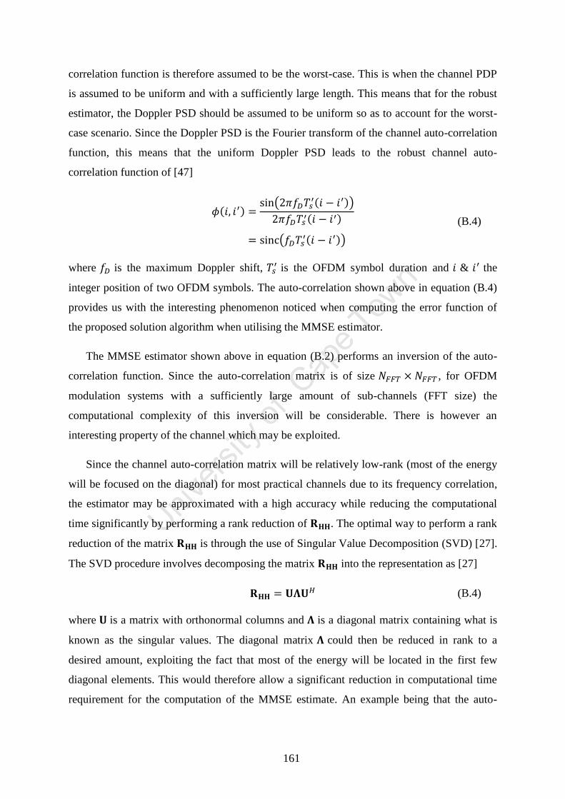
161

correlation function is therefore assumed to be the worst-case. This is when the channel PDP

is assumed to be uniform and with a sufficiently large length. This means that for the robust

estimator, the Doppler PSD should be assumed to be uniform so as to account for the worst-

case scenario. Since the Doppler PSD is the Fourier transform of the channel auto-correlation

function, this means that the uniform Doppler PSD leads to the robust channel auto-

correlation function of [47]

where is the maximum Doppler shift, is the OFDM symbol duration and & the

integer position of two OFDM symbols. The auto-correlation shown above in equation (B.4)

provides us with the interesting phenomenon noticed when computing the error function of

the proposed solution algorithm when utilising the MMSE estimator.

The MMSE estimator shown above in equation (B.2) performs an inversion of the auto-

correlation function. Since the auto-correlation matrix is of size , for OFDM

modulation systems with a sufficiently large amount of sub-channels (FFT size) the

computational complexity of this inversion will be considerable. There is however an

interesting property of the channel which may be exploited.

Since the channel auto-correlation matrix will be relatively low-rank (most of the energy

will be focused on the diagonal) for most practical channels due to its frequency correlation,

the estimator may be approximated with a high accuracy while reducing the computational

time significantly by performing a rank reduction of . The optimal way to perform a rank

reduction of the matrix is through the use of Singular Value Decomposition (SVD) [27].

The SVD procedure involves decomposing the matrix into the representation as [27]

where is a matrix with orthonormal columns and is a diagonal matrix containing what is

known as the singular values. The diagonal matrix could then be reduced in rank to a

desired amount, exploiting the fact that most of the energy will be located in the first few

diagonal elements. This would therefore allow a significant reduction in computational time

requirement for the computation of the MMSE estimate. An example being that the auto-

( )

( )

(B.4)

(B.4)

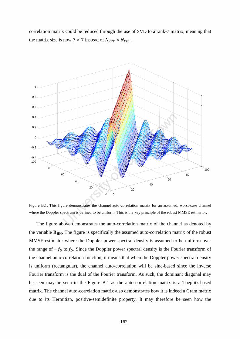
162

correlation matrix could be reduced through the use of SVD to a rank-7 matrix, meaning that

the matrix size is now instead of .

Figure B.1. This figure demonstrates the channel auto-correlation matrix for an assumed, worst-case channel

where the Doppler spectrum is defined to be uniform. This is the key principle of the robust MMSE estimator.

The figure above demonstrates the auto-correlation matrix of the channel as denoted by

the variable . The figure is specifically the assumed auto-correlation matrix of the robust

MMSE estimator where the Doppler power spectral density is assumed to be uniform over

the range of to . Since the Doppler power spectral density is the Fourier transform of

the channel auto-correlation function, it means that when the Doppler power spectral density

is uniform (rectangular), the channel auto-correlation will be sinc-based since the inverse

Fourier transform is the dual of the Fourier transform. As such, the dominant diagonal may

be seen may be seen in the Figure B.1 as the auto-correlation matrix is a Toeplitz-based

matrix. The channel auto-correlation matrix also demonstrates how it is indeed a Gram matrix

due to its Hermitian, positive-semidefinite property. It may therefore be seen how the

0

20

40

60

80

100

0

20

40

60

80

100

-0.4

-0.2

0

0.2

0.4

0.6

0.8

1

163

complexity reduction of the MMSE estimator through the use of singular value

decomposition is indeed a very effective way to reduce the computational time requirement

of the estimator since most of the energy of the auto-correlation matrix is indeed based

around the diagonal of the matrix.

164

Appendix C: Analysis of polynomial interpolant error bound

When using any channel estimator, there needs to be some way to interpolate the

measured channel gains at pilot symbol positions to data symbol positions. The MMSE

estimator uses the Wiener FIR filter to perform an MMSE interpolation, the LS estimator on

the other hand has several different types of interpolations which may be used. The most

common type of interpolation is the linear (1st order) and the polynomial (higher order)

interpolators.

In order to perform an analysis on the error bounds as well as performance of several

higher-order interpolants, it is first necessary to derive these interpolants. The 2nd

and 3rd

order polynomial interpolators will be demonstrated in this section as well as compared to the

linear (1st order) interpolator when analysing the performance of these interpolators.

The 2nd

order interpolator is derived from the generalised polynomial expression of the

form

where is the polynomial coefficient and interpolates the signal from the set of

provided data points (or sample points) at positions such that

The purpose of the polynomial interpolators is therefore to find the set of coefficients

which would best fit the desired input data in the least squares sense. From this we can

therefore form the 2nd

and 3rd

order polynomial interpolators as [32]

The set of equations above can be formulated as a matrix of the form [32]

(C.1)

(C.2)

(C.3)

[

] [

] [

] (C.4)

165

where the purpose of the interpolation is to fit the coefficients vector containing the

values so as to minimise error in the least squares sense. This can be represented as

and therefore to obtain the polynomial interpolant in the least squares sense, we do an

inversion and multiplication of X as follows

Depending on the channel frequency response, the coefficient values for the interpolant

will differ for every OFDM symbol. It would therefore require the polynomial interpolator

coefficients to be calculated for every new OFDM symbol. For channels with a relatively

large coherent time compared to the OFDM symbol duration, these coefficients will vary at

the same rate as the CIR/CFR. This means that a matrix inversion will need to be computed

for, at the worst case, every OFDM symbol. As the matrix size is the square of the

interpolation polynomial order, this means that the computational complexity will increase

exponentially (square) with the increase of the interpolator order.

(C.5)

(C.6)

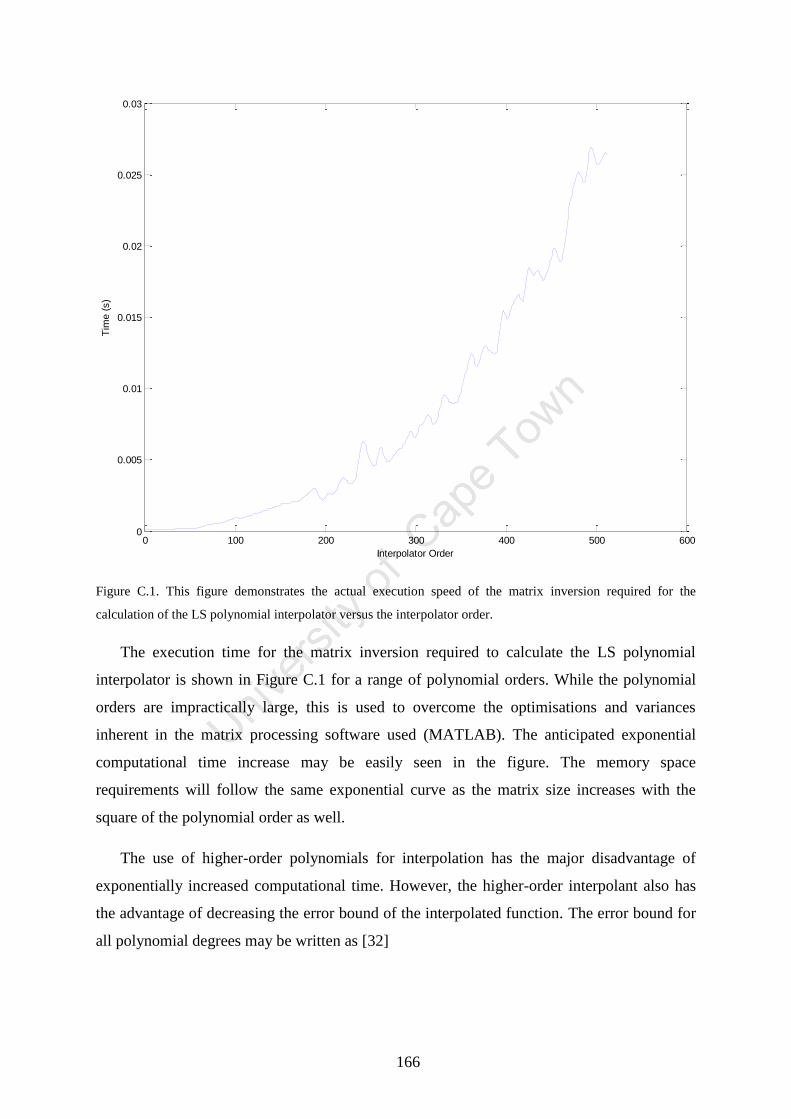
166

Figure C.1. This figure demonstrates the actual execution speed of the matrix inversion required for the

calculation of the LS polynomial interpolator versus the interpolator order.

The execution time for the matrix inversion required to calculate the LS polynomial

interpolator is shown in Figure C.1 for a range of polynomial orders. While the polynomial

orders are impractically large, this is used to overcome the optimisations and variances

inherent in the matrix processing software used (MATLAB). The anticipated exponential

computational time increase may be easily seen in the figure. The memory space

requirements will follow the same exponential curve as the matrix size increases with the

square of the polynomial order as well.

The use of higher-order polynomials for interpolation has the major disadvantage of

exponentially increased computational time. However, the higher-order interpolant also has

the advantage of decreasing the error bound of the interpolated function. The error bound for

all polynomial degrees may be written as [32]

0 100 200 300 400 500 6000

0.005

0.01

0.015

0.02

0.025

0.03

Interpolator Order

Tim

e (

s)

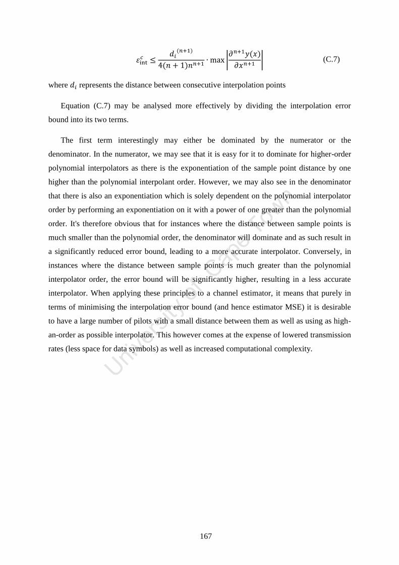
167

where represents the distance between consecutive interpolation points

Equation (C.7) may be analysed more effectively by dividing the interpolation error

bound into its two terms.

The first term interestingly may either be dominated by the numerator or the

denominator. In the numerator, we may see that it is easy for it to dominate for higher-order

polynomial interpolators as there is the exponentiation of the sample point distance by one

higher than the polynomial interpolant order. However, we may also see in the denominator

that there is also an exponentiation which is solely dependent on the polynomial interpolator

order by performing an exponentiation on it with a power of one greater than the polynomial

order. It's therefore obvious that for instances where the distance between sample points is

much smaller than the polynomial order, the denominator will dominate and as such result in

a significantly reduced error bound, leading to a more accurate interpolator. Conversely, in

instances where the distance between sample points is much greater than the polynomial

interpolator order, the error bound will be significantly higher, resulting in a less accurate

interpolator. When applying these principles to a channel estimator, it means that purely in

terms of minimising the interpolation error bound (and hence estimator MSE) it is desirable

to have a large number of pilots with a small distance between them as well as using as high-

an-order as possible interpolator. This however comes at the expense of lowered transmission

rates (less space for data symbols) as well as increased computational complexity.

|

| (C.7)

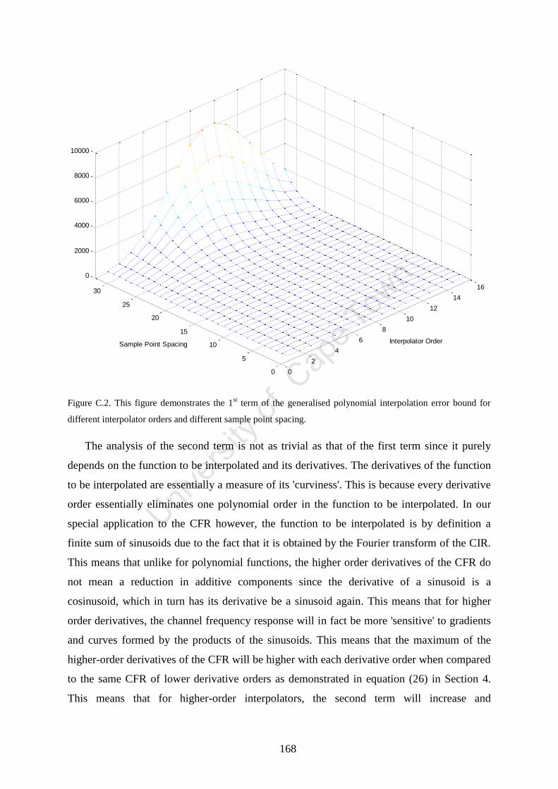
168

Figure C.2. This figure demonstrates the 1st term of the generalised polynomial interpolation error bound for

different interpolator orders and different sample point spacing.

The analysis of the second term is not as trivial as that of the first term since it purely

depends on the function to be interpolated and its derivatives. The derivatives of the function

to be interpolated are essentially a measure of its 'curviness'. This is because every derivative

order essentially eliminates one polynomial order in the function to be interpolated. In our

special application to the CFR however, the function to be interpolated is by definition a

finite sum of sinusoids due to the fact that it is obtained by the Fourier transform of the CIR.

This means that unlike for polynomial functions, the higher order derivatives of the CFR do

not mean a reduction in additive components since the derivative of a sinusoid is a

cosinusoid, which in turn has its derivative be a sinusoid again. This means that for higher

order derivatives, the channel frequency response will in fact be more 'sensitive' to gradients

and curves formed by the products of the sinusoids. This means that the maximum of the

higher-order derivatives of the CFR will be higher with each derivative order when compared

to the same CFR of lower derivative orders as demonstrated in equation (26) in Section 4.

This means that for higher-order interpolators, the second term will increase and

0

2

4

6

8

10

12

14

16

0

5

10

15

20

25

30

0

2000

4000

6000

8000

10000

Interpolator OrderSample Point Spacing

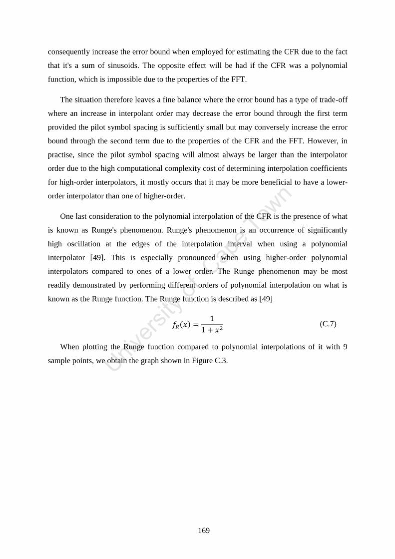
169

consequently increase the error bound when employed for estimating the CFR due to the fact

that it's a sum of sinusoids. The opposite effect will be had if the CFR was a polynomial

function, which is impossible due to the properties of the FFT.

The situation therefore leaves a fine balance where the error bound has a type of trade-off

where an increase in interpolant order may decrease the error bound through the first term

provided the pilot symbol spacing is sufficiently small but may conversely increase the error

bound through the second term due to the properties of the CFR and the FFT. However, in

practise, since the pilot symbol spacing will almost always be larger than the interpolator

order due to the high computational complexity cost of determining interpolation coefficients

for high-order interpolators, it mostly occurs that it may be more beneficial to have a lower-

order interpolator than one of higher-order.

One last consideration to the polynomial interpolation of the CFR is the presence of what

is known as Runge's phenomenon. Runge's phenomenon is an occurrence of significantly

high oscillation at the edges of the interpolation interval when using a polynomial

interpolator [49]. This is especially pronounced when using higher-order polynomial

interpolators compared to ones of a lower order. The Runge phenomenon may be most

readily demonstrated by performing different orders of polynomial interpolation on what is

known as the Runge function. The Runge function is described as [49]

When plotting the Runge function compared to polynomial interpolations of it with 9

sample points, we obtain the graph shown in Figure C.3.

(C.7)

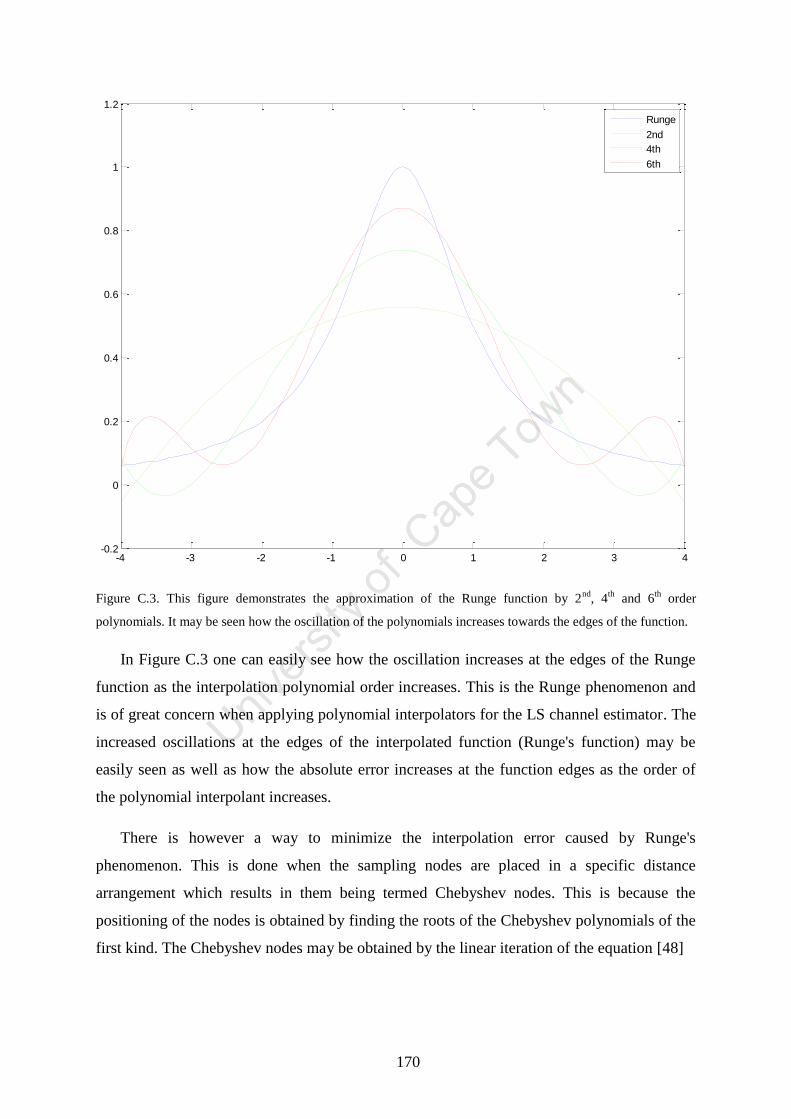
170

Figure C.3. This figure demonstrates the approximation of the Runge function by 2nd

, 4th

and 6th

order

polynomials. It may be seen how the oscillation of the polynomials increases towards the edges of the function.

In Figure C.3 one can easily see how the oscillation increases at the edges of the Runge

function as the interpolation polynomial order increases. This is the Runge phenomenon and

is of great concern when applying polynomial interpolators for the LS channel estimator. The

increased oscillations at the edges of the interpolated function (Runge's function) may be

easily seen as well as how the absolute error increases at the function edges as the order of

the polynomial interpolant increases.

There is however a way to minimize the interpolation error caused by Runge's

phenomenon. This is done when the sampling nodes are placed in a specific distance

arrangement which results in them being termed Chebyshev nodes. This is because the

positioning of the nodes is obtained by finding the roots of the Chebyshev polynomials of the

first kind. The Chebyshev nodes may be obtained by the linear iteration of the equation [48]

-4 -3 -2 -1 0 1 2 3 4-0.2

0

0.2

0.4

0.6

0.8

1

1.2

Runge

2nd

4th

6th

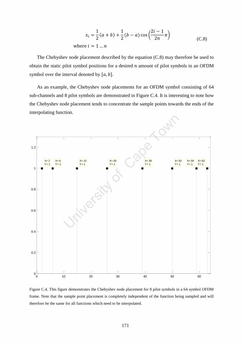
171

The Chebyshev node placement described by the equation (C.8) may therefore be used to

obtain the static pilot symbol positions for a desired amount of pilot symbols in an OFDM

symbol over the interval denoted by [ ].

As an example, the Chebyshev node placements for an OFDM symbol consisting of 64

sub-channels and 8 pilot symbols are demonstrated in Figure C.4. It is interesting to note how

the Chebyshev node placement tends to concentrate the sample points towards the ends of the

interpolating function.

Figure C.4. This figure demonstrates the Chebyshev node placement for 8 pilot symbols in a 64 symbol OFDM

frame. Note that the sample point placement is completely independent of the function being sampled and will

therefore be the same for all functions which need to be interpolated.

0 10 20 30 40 50 600

0.2

0.4

0.6

0.8

1

1.2

X= 2

Y= 1

X= 6

Y= 1

X= 15

Y= 1

X= 26

Y= 1

X= 39

Y= 1

X= 50

Y= 1

X= 59

Y= 1

X= 63

Y= 1

(

)

(C.8)

172

It is for the reason of the Chebyshev node placements that a higher-order polynomial

interpolator may be undesirable for the practical implementation of a channel estimator since

it would result in a large proportion of the pilot symbols being placed on the edges of the

OFDM symbol. This means that for sub-channels in the centre, there will be a higher MSE

due to the sparser sampling of the CFR. This is very difficult to remedy as there is a limited

power budget in terms of how many pilot symbols may be placed in an OFDM symbol as

well as the reduction in transmissions throughput with the replacement of each data symbol

with a pilot symbol.

173

Appendix D: Different terrain types when modelling channels

When modelling channels, it is necessary to have a basis for creating the models which is

derived from the majority of practical situations for the application required. The purpose is

to obtain a wide variety of the different situations in which the desired communications

system would be used by its users. As such, for most fixed wireless applications, the terrain

conditions may be characterised as [40]:

Path loss

Multipath delay spread

Fading characteristics

Doppler spread

Co-channel and adjacent channel interference

These parameters used to describe the channels and the subsequent channel models which

may be derived from them are in fact only statistical models and the actual values of the

parameters are always random. The channel models then comprise of statistical models

specifying the PDFs, means and variances of the channel characteristics.

The channel models used by the IEEE 802.16 WiMAX committee are based on the

modified SUI models as specified in [40]. The channel model's median path loss may be

effectively summarised by the equation

The variables in equation (D.1) are described as being the logarithmic decibel factor

modelled as

with being the transmitted signal wavelength of the transmitted signal in metres and

being the close-in distance in metres as well.

Another factor represented in equation (D.1) is the path-loss exponent denoted by and

mathematically derived as

(

)

(D.1)

(

) (D.2)

174

where is considered to be the base-station height denoted in metres while the factors ,

and representing the factors used to model different terrain types summarised by the table

below [40].

Table D.4. Channel model parameters by different terrain types.

Model Parameter Type A Type B Type C

4.6 4 3.6

0.0075 0.0065 0.005

12.6 17.1 20

Lastly, the value denoted by in equation (D.1) represents the shadowing component

adding to the path loss. This value usually ranges between 8.2 and 10.6 dB depending on the

type of terrain as well as tree density present in the terrain used for the transmission of the

wireless signals.

(

) (D.3)

175

Appendix E: Mathematical description of Rician and Rayleigh fading

The fading undergone by a signal when transmitted through a channel may be

characterised by its time-based effects and its frequency-based effects. Since the channel may

be modelled as a finite impulse-response filter, the instantaneous effects of the channel may

be characterised either by its impulse response or frequency response.

The channel impulse response may be seen as a set of transmitted pulses (although in

practise it is continuous) with an envelope which may be formed over these impulses. It is

this envelope that characterises the CIR into different fading distributions. The envelope

usually conforms to Rayleigh or Rician probability distributions depending on the channel

conditions and environment.

The Rayleigh PDF can be modelled as [44]

where is the mean signal power and is the instantaneously received signal. It should be

noted that the received signal is equivalent to the received signal envelope defined by [44]

with and being the in-phase and quadrature components respectively of the transmitted

signal .

The probability of the fading envelope of the channel may then be integrated to obtain the

cumulative distribution function (CDF) so that the probability of the fading maintains a fixed

threshold/value below or equal to may be mathematically formulated as [44]

where is the desired level for which the probability of the signal being less than or equal to

may be obtained by equation (E.3).

(

) (E.1)

√ (E.2)

∫

(

)

(E.3)

176

The mean value (or equivalently the expectation) of the Rayleigh fading envelope may be

characterised by the equation [44]

The mean square value of the Rayleigh fading may also be characterised by

And the variance of the Rayleigh fading envelope defined as

The Rayleigh distribution described in the equations above may then be further

generalised into what is known as the Rician distribution. The Rayleigh distribution is

actually a special case of the Rician distribution where one of the properties of the Rician

distribution, known as the K-factor, is set to zero. The Rician distribution probability density

function is mathematically noted as

In equation (E.7), K is the Rician K-factor in decibels, is the power of the dominant

(i.e. first in arrival) signal and represents the 0th

order modified Bessel function of the first

kind.

The Rician K-factor can be related to the power of the dominant signal by the expression

{ }

∫

√

(E.4)

{ } ∫

(E.5)

{ } { }

(

)

(E.6)

(

) (

) (E.7)

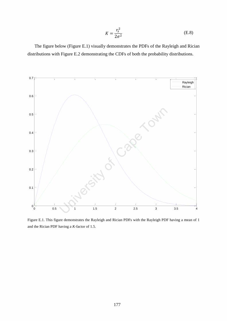
177

The figure below (Figure E.1) visually demonstrates the PDFs of the Rayleigh and Rician

distributions with Figure E.2 demonstrating the CDFs of both the probability distributions.

Figure E.1. This figure demonstrates the Rayleigh and Rician PDFs with the Rayleigh PDF having a mean of 1

and the Rician PDF having a K-factor of 1.5.

0 0.5 1 1.5 2 2.5 3 3.5 40

0.1

0.2

0.3

0.4

0.5

0.6

0.7

Rayleigh

Rician

(E.8)

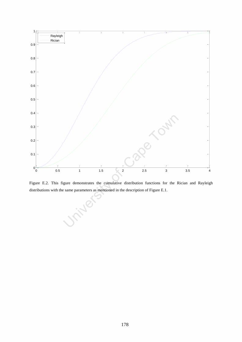
178

Figure E.2. This figure demonstrates the cumulative distribution functions for the Rician and Rayleigh

distributions with the same parameters as mentioned in the description of Figure E.1.

0 0.5 1 1.5 2 2.5 3 3.5 40

0.1

0.2

0.3

0.4

0.5

0.6

0.7

0.8

0.9

1

Rayleigh

Rician