Embed Size (px)
Citation preview
Pit Optimization on the Efficient Frontier
by
Tyler Acorn
A thesis submi ed in partial fulfillment of the requirements for the degree of
Master of Science
in
Mining Engineering
Department of Civil and Environmental EngineeringUniversity of Alberta
© Tyler Acorn, 2017

AThe mining industry has become increasingly concerned with the effects of uncertainty and risk
in resource modeling. Some companies are moving away from deterministic geologic modeling
techniques to approaches that quantify uncertainty. Stochastic modeling techniques produce mul-
tiple realizations of the geologic model to quantify uncertainty, but integrating these results into
pit optimization is non-trivial.
Conventional pit optimization calculates optimal pit limits from a block model of economic val-
ues and precedence rules for pit slopes. There are well established algorithms for this including
Lerchs-Grossmann, push-relabel and pseudo-flow; however, these conventional optimizers have
limited options for handling stochastic block models. The conventional optimizers could be mod-
ified to incorporate a block-by-block penalty based on uncertainty, but not uncertainty in the re-
source within the entire pit.
There is a need for a new pit limit optimizing algorithm that would consider multiple block
model realizations. To address risk management principles in the pit shell optimization stage, a
novel approach is presented for optimizing pit shells over all realizations. The inclusion of mul-
tiple realizations provides access to summary statistics across the realizations such as the risk or
uncertainty in the pit value. This permits an active risk management approach.
A heuristic pit optimization algorithm is proposed to target the joint uncertainty between mul-
tiple input models. A practical framework is presented for actively managing the risk by adapting
Harry Markowi ’s “Efficient Frontier” approach to pit shell optimization. Choosing the accept-
able level of risk along the frontier can be subjective. A risk-rating modification is proposed to
minimize some of the subjectivity in choosing the acceptable level of risk. The practical application
of the framework using the heuristic pit optimization algorithm is demonstrated through multiple
case studies.
ii

D“The more I learn, the more I realize how much I don’t know.”
- Albert Einstein
“42”
- Douglas Adams The Hitchhiker’s Guide to the Galaxy
iii

AI would like to first thank my partner, Merilie Reynolds, for her support and dedication to contin-
uing to question and support our paths through life. Without her I would not be here finishing a
thesis in geostatistics. She is one of the kindest individuals I know and her intellect is beautiful to
watch. Secondly, I would like to thank my advisor, Dr. Clayton Deutsch. Clayton leads through
example, and somehow pushes all of us to excel beyond what we thought possible; partly through
his joy of geostatistics and partly through some magic that we never quite figured out. He is one of
the best examples of leading that I have had the pleasure of working with. Clayton’s sharp mind,
amazing memory, and patience with all of us will continue to inspire me for a long time to come.
I would also like to thank all my colleagues at the Centre for Computation Geostatistics. Jared,
for introducing me to the wonderful world of Python. Warren, for his willingness to plunge deeper
into the rabbit hole. Ryan for your amazing automatic compiling scripts and your everyday appar-
ent joy in life. Felipe, for your friendship and willingness to answer any question I throw your way.
Dr. Manchuk, for helping me improve my coding skills. I have throughly enjoyed working with
all of the other researchers here at CCG and feel blessed to have been able to work with everyone
these past couple of years.
iv

T C
1 Introduction 1
1.1 Motivation for Risk Management in Optimizing Pit Limits . . . . . . . . . . . . . . . 1
1.2 Scope of the Research . . . . . . . . . . . . . . . . . . . . . . . . . . . . . . . . . . . . . 2
1.3 Overview of Thesis Chapters . . . . . . . . . . . . . . . . . . . . . . . . . . . . . . . . 2
2 Review of Key Ideas and Terminology 4
2.1 Resource Modeling . . . . . . . . . . . . . . . . . . . . . . . . . . . . . . . . . . . . . . 4
2.1.1 Deterministic Paradigm . . . . . . . . . . . . . . . . . . . . . . . . . . . . . . . 6
2.1.2 Stochastic Paradigm . . . . . . . . . . . . . . . . . . . . . . . . . . . . . . . . . 6
2.2 Defining Pit Shells and Mine Planning . . . . . . . . . . . . . . . . . . . . . . . . . . . 7
2.2.1 Ultimate Pit Shells and the Staging of Pits . . . . . . . . . . . . . . . . . . . . . 8
2.2.2 Common Algorithms For Determining Pit Shells . . . . . . . . . . . . . . . . . 9
2.3 Management of Risk . . . . . . . . . . . . . . . . . . . . . . . . . . . . . . . . . . . . . 10
2.4 Pit Optimization in the Presence of Risk . . . . . . . . . . . . . . . . . . . . . . . . . . 11
2.4.1 Passive Paradigm . . . . . . . . . . . . . . . . . . . . . . . . . . . . . . . . . . . 11
2.4.2 Active Paradigm . . . . . . . . . . . . . . . . . . . . . . . . . . . . . . . . . . . 12
3 Development of a Heuristic Pit Optimizer 14
3.1 Motivation . . . . . . . . . . . . . . . . . . . . . . . . . . . . . . . . . . . . . . . . . . . 14
3.1.1 Limitations in Commercial Pit Optimizers . . . . . . . . . . . . . . . . . . . . 15
3.1.2 Limitations in Other Pit Optimizers . . . . . . . . . . . . . . . . . . . . . . . . 15
3.2 Proposed Algorithm . . . . . . . . . . . . . . . . . . . . . . . . . . . . . . . . . . . . . 16
3.2.1 Iteratively Find and Modify Solutions . . . . . . . . . . . . . . . . . . . . . . . 17
3.2.2 Calculating The Objective Function . . . . . . . . . . . . . . . . . . . . . . . . 17
3.3 The Heuristic Pit Optimizer . . . . . . . . . . . . . . . . . . . . . . . . . . . . . . . . . 19
3.3.1 Input and Parameters . . . . . . . . . . . . . . . . . . . . . . . . . . . . . . . . 20
3.3.2 Preprocessing the Data . . . . . . . . . . . . . . . . . . . . . . . . . . . . . . . . 21
3.3.3 Finding and Modifying Solutions . . . . . . . . . . . . . . . . . . . . . . . . . 22
3.3.4 Reviewing the Objective Function . . . . . . . . . . . . . . . . . . . . . . . . . 24
3.4 Alternatives in the Objective Function . . . . . . . . . . . . . . . . . . . . . . . . . . . 25
4 Testing the Heuristic Pit Optimizer 26
4.1 Testing with a Two-Dimensional Model . . . . . . . . . . . . . . . . . . . . . . . . . . 26
4.1.1 HPO Compared to LG3D . . . . . . . . . . . . . . . . . . . . . . . . . . . . . . . . 27
4.1.2 Testing with Multiple Input Models . . . . . . . . . . . . . . . . . . . . . . . . 28
v

Table of Contents
4.2 Testing with a Three-Dimensional Model . . . . . . . . . . . . . . . . . . . . . . . . . 29
4.2.1 Visual Checks and Comparing against LG3D . . . . . . . . . . . . . . . . . . . 30
4.2.2 Testing with a Single Input Model . . . . . . . . . . . . . . . . . . . . . . . . . 32
4.2.3 Testing with Multiple Input Models . . . . . . . . . . . . . . . . . . . . . . . . 33
4.3 Computation Costs . . . . . . . . . . . . . . . . . . . . . . . . . . . . . . . . . . . . . . 34
4.4 Optimality of HPO and Tuning Parameters . . . . . . . . . . . . . . . . . . . . . . . . . 35
5 The Efficient Frontier for Pit Optimization 38
5.1 Adapting the Efficient Frontier to Pit Optimization with Risk-Rated Contours . . . . 38
5.2 Overview of the Case Study Models . . . . . . . . . . . . . . . . . . . . . . . . . . . . 41
5.3 Finding the Efficient Frontier . . . . . . . . . . . . . . . . . . . . . . . . . . . . . . . . 42
5.3.1 Efficient Frontier for the 2-D Case Study . . . . . . . . . . . . . . . . . . . . . . 43
5.3.2 Efficient Frontier for the Small 3-D Case Study . . . . . . . . . . . . . . . . . . 44
5.3.3 Efficient Frontier for the Medium 3-D Case Study . . . . . . . . . . . . . . . . 45
5.4 Using the Risk-Rated Contours for Be er Informed Decisions . . . . . . . . . . . . . 46
5.4.1 Managing Risk for the 2-D Case Study . . . . . . . . . . . . . . . . . . . . . . . 47
5.4.2 Managing Risk for the Small 3-D Case Study . . . . . . . . . . . . . . . . . . . 48
5.4.3 Managing Risk for the Medium 3-D Case Study . . . . . . . . . . . . . . . . . 49
5.5 Reviewing Changes in the Frontier Pits for the Medium 3-D Case Study . . . . . . . 51
5.6 Comparing Pits Along the Efficient Frontier to Traditional Results . . . . . . . . . . . 55
6 Conclusion 58
6.1 Contributions . . . . . . . . . . . . . . . . . . . . . . . . . . . . . . . . . . . . . . . . . 58
6.2 Some Generalizations about the Efficient Frontier for Pit Optimization . . . . . . . . 58
6.3 Future Work . . . . . . . . . . . . . . . . . . . . . . . . . . . . . . . . . . . . . . . . . . 60
6.3.1 Suggestions to Improve the Optimization Algorithm . . . . . . . . . . . . . . 60
6.3.2 Suggestions for Future Research Applying the HPO Algorithm . . . . . . . . . 62
6.4 Recommendations . . . . . . . . . . . . . . . . . . . . . . . . . . . . . . . . . . . . . . 63
References 64
A Appendices 68
A.1 Description of All Parameters in the Heuristic Pit Optimizer . . . . . . . . . . . . . . 68
A.1.1 MAIN: . . . . . . . . . . . . . . . . . . . . . . . . . . . . . . . . . . . . . . . . . 70
A.1.2 OBJ_FUNCT: . . . . . . . . . . . . . . . . . . . . . . . . . . . . . . . . . . . . . 70
A.1.3 GLOBAL_OPTIMA: . . . . . . . . . . . . . . . . . . . . . . . . . . . . . . . . . 71
A.1.4 PRECEDANCE: . . . . . . . . . . . . . . . . . . . . . . . . . . . . . . . . . . . . 71
A.1.5 FILE FORMATS: . . . . . . . . . . . . . . . . . . . . . . . . . . . . . . . . . . . 72
vi

Table of Contents
A.1.6 DEBUG: . . . . . . . . . . . . . . . . . . . . . . . . . . . . . . . . . . . . . . . . 72
A.2 Note on the Use of Multiple Economic Block Models . . . . . . . . . . . . . . . . . . . 72
A.3 Website Information for Reviewed Commercial Software . . . . . . . . . . . . . . . . 74
vii

L T2.1 Survey of algorithms used in commercial pit optimization software . . . . . . . . . . . . 10
4.1 2D test results with multiple input models . . . . . . . . . . . . . . . . . . . . . . . . . . 29
5.1 Percent change of values in 2-D case study options . . . . . . . . . . . . . . . . . . . . . . 48
5.2 Percent change of values in small 3-D case study options . . . . . . . . . . . . . . . . . . 49
5.3 Percent change of values in medium 3-D case study options . . . . . . . . . . . . . . . . 51
A.1 Website of commercial pit optimization software . . . . . . . . . . . . . . . . . . . . . . . 75
viii

L F2.1 A simplified work flow for the resource modeling process . . . . . . . . . . . . . . . . . 4
2.2 Schematic of the efficient frontier . . . . . . . . . . . . . . . . . . . . . . . . . . . . . . . . 11
3.1 HPO program overview . . . . . . . . . . . . . . . . . . . . . . . . . . . . . . . . . . . . . . 19
3.2 Vertical grid used in HPO . . . . . . . . . . . . . . . . . . . . . . . . . . . . . . . . . . . . . 20
3.3 Precedence block rule sets . . . . . . . . . . . . . . . . . . . . . . . . . . . . . . . . . . . . 21
3.4 HPO boundary types . . . . . . . . . . . . . . . . . . . . . . . . . . . . . . . . . . . . . . . . 22
3.5 Perturbations function flow chart . . . . . . . . . . . . . . . . . . . . . . . . . . . . . . . . 23
4.1 Comparison of HPO to LG3D pit shell limits . . . . . . . . . . . . . . . . . . . . . . . . . . . 27
4.2 Comparing HPO and LG3D pit values . . . . . . . . . . . . . . . . . . . . . . . . . . . . . . 28
4.3 North-South cross-sections of 3-D model used for visual checks . . . . . . . . . . . . . . 30
4.4 Expected value model pit shell 3-D view . . . . . . . . . . . . . . . . . . . . . . . . . . . . 31
4.5 Compare HPO pit values to LG3D pit values in 3-D test case . . . . . . . . . . . . . . . . . . 32
4.6 Pit values box plots for a single 3-D model organized by number of restart locations . . 33
4.7 Pit values box plots for a single 3-D model organized by number of random restarts . . 34
4.8 HPO 3-D test results for multiple input models . . . . . . . . . . . . . . . . . . . . . . . . . 35
4.9 HPO runtime . . . . . . . . . . . . . . . . . . . . . . . . . . . . . . . . . . . . . . . . . . . . 36
5.1 A schematic of The efficient frontier . . . . . . . . . . . . . . . . . . . . . . . . . . . . . . 38
5.2 An asymmetrical utility function . . . . . . . . . . . . . . . . . . . . . . . . . . . . . . . . 39
5.3 Illustration of the risk-rated contour . . . . . . . . . . . . . . . . . . . . . . . . . . . . . . 40
5.4 Illustration of the risk-rated contours with secondary abscissa axis . . . . . . . . . . . . 40
5.5 The efficient frontier for the 2-D synthetic model . . . . . . . . . . . . . . . . . . . . . . . 44
5.6 Side view plot of the maximum expected value pit for the 2-D synthetic model . . . . . 44
5.7 The efficient frontier for the small 3-D case study . . . . . . . . . . . . . . . . . . . . . . . 45
5.8 Surface plot of the maximum expected value pit for the small model . . . . . . . . . . . 45
5.9 The efficient frontier for the medium 3-D case study . . . . . . . . . . . . . . . . . . . . . 46
5.10 Surface plot of the maximum expected value pit for the medium 3-D case study . . . . . 46
5.11 Risk-rated contours for the 2-D case study . . . . . . . . . . . . . . . . . . . . . . . . . . . 47
5.12 Risk-rated contours for the small case study . . . . . . . . . . . . . . . . . . . . . . . . . . 48
5.13 An example of noisy risk-rated contours for the medium 3-D case study . . . . . . . . . 50
5.14 Risk-rated contours for the medium case study . . . . . . . . . . . . . . . . . . . . . . . . 50
5.15 Surface plots of the reference pit and delta surfaces for the medium case study . . . . . 52
5.16 North-South cross-sections of the medium case study . . . . . . . . . . . . . . . . . . . . 53
ix

List of Figures
5.17 East-West cross-sections of the medium case study . . . . . . . . . . . . . . . . . . . . . . 54
5.18 Expected pit value versus risk of traditional pit shells . . . . . . . . . . . . . . . . . . . . 56
6.1 Schematic generalizations of the efficient frontier . . . . . . . . . . . . . . . . . . . . . . . 59
A.1 Simplified grade transfer function . . . . . . . . . . . . . . . . . . . . . . . . . . . . . . . 72
A.2 CDF’s of expected block value models from different grade transfer functions . . . . . . 74
x

L S
Symbol Description
CumulativeYx,y,z,l Cumulative block value for block ux,y,z,l considering all blocks directly above
E[ ] Expected value
gi Block grade at location i
gz Economic cut-off grade
i Indexer for summation
I Total number of blocks inside pit shell
l Block model index
L Total number of input models
ωpv Risk penalization factor applied to the risk measurement for the pit value
Rpv Measure of risk (standard deviation) of the pit value
σ Standard deviation
V (u; l) Block value at location u, for realization l
V u Average block value at location u
Vp(l) Value of a pit shell evaluated on realization l
Vp Value of a pit shell evaluated and averaged over all realizations
x x-axis index for blocks in the block model
y y-axis index for blocks in the block model
z z-axis index for blocks in the block model
Z Total number of blocks in z-axis of the block model
z(u; k, l) Random value at location u, with k grade, for realization l
xi

L A
Abbreviation Description
2-D Two-dimensional
3-D Three-dimensional
CDF Cumulative distribution function
GSLIB Geostatistical software library
HPO Heuristic pit optimizer
NPV Net present value
xii

C 1
IIn surface mining operations the optimization of pit shells is an important step in evaluation and
planning. The ultimate pit shell is the maximum value pit based on the geologic model, engineering
and economic parameters. There are many techniques addressing this problem using determinis-
tic block models. However, at the pit optimization stage there are limited options for handling
stochastic block models and no clear approach for addressing uncertainty in the geologic models.
Uncertainty in the geologic models is inevitable because the available data is relatively sparse
and the geologic knowledge of the deposit is always incomplete. Traditionally, deterministic tech-
niques such as inverse distance and kriging have been used to model the resources and reserves of
a deposit. These techniques result in one model of the “best” estimate of grade for each location.
Recent geostatistical research has focused on understanding and viewing the uncertainty in a
geologic model. This is often done using stochastic modeling techniques that produce multiple real-
izations of the model. The uncertainty in the geologic models will effect downstream processes such
as ultimate pit shell boundaries. Seeking to understand and manage the uncertainty in ultimate pit
shell boundaries is a logical next step.
1.1 Motivation for Risk Management in Optimizing Pit Limits
Risk and uncertainty should be understood and managed during all stages of an investment. Since
at least the time of Daniel Bernoulli and his pioneering work on risk in the 1700’s (Bernoulli, 1738/1954),
there have been many expositions on making the best decision in the presence of risk. A basic tenant
of risk management is that risk could change the optimal decision.
The algorithms currently available in commercial pit optimization software either account for
uncertainty with a passive approach or consider uncertainty for each block one at a time. Some aca-
demic algorithms focus on optimizing production schedules, but not with all realizations. Multiple
realizations of the geologic model are easily generated. These realizations need to be summarized
by a single model to be used as input for most mine design software. In summarizing all realiza-
tions in a single block model, information about the joint uncertainty in large production volumes
is lost and therefore cannot be accounted for by the optimizers.
Much of the current geostatistical research has gone into understanding and viewing the un-
certainty in a geostatistical project by switching from the deterministic approach to stochastic tech-
niques. While work is ongoing in this area, the next logical step is to seek to understand and manage
the uncertainty transferred from the geologic models to the risk in downstream processes such as
1
1. Introduction
optimizing the pit shell boundaries.
1.2 Scope of the Research
This research contributes through the development of an algorithm for optimizing pit shells over
all realizations. The goal is to account for the joint uncertainty in the grade models and mitigate the
reserve risk within pit shells. A framework is developed for the practical application of an active
risk management approach to pit shell optimization.
The optimization process proposed in this research is designed for simplicity and flexibility.
Heuristics and random paths are used to find optimal solutions to maximizing the expected pit
value for all input models. Penalization factors in the objective function manage the uncertainty in
the input models. The objective function can be expanded to include other optimization goals.
The proposed algorithm is a new approach to optimizing pit shells. Some testing is done in both
single and multiple model cases. The single model cases will be used to compare the results of the
algorithm to traditional approaches such as the Lerchs-Grossman algorithm. The multiple model
test case shows the validity of the algorithm as a concept for optimizing over all realizations.
The second part of this research is the practical use of the algorithm. A framework is presented
for actively managing the risk in the pit shell optimization stage. Risk is an important aspect of any
venture that should be understood and managed. Managing risk is especially important for very
expensive mining projects that can span decades.
A method for understanding and managing risk comes from portfolio theory and was proposed
by Markowi (1952) with his idea of the efficient frontier for portfolio selection. This risk manage-
ment approach is modified here for a pit shell optimization workflow. In an a empt to decrease
some of the objectivity in choosing an acceptable level of risk along the frontier, a risk-rating mod-
ification is proposed. Together the efficient frontier and the risk-rated contours show a practical
workflow for actively managing the risk in pit shell optimization.
1.3 Overview of Thesis Chapters
The remainder of this thesis is organized in five additional chapters. These chapters will present the
algorithm developed for optimizing over multiple input models and the active risk management
approach developed for choosing between available options in the optimized pit shells.
Before presenting the proposed optimization algorithm, Chapter 2 will review some key ideas
related to the research in this thesis. The review will present some of the current methods for geo-
statistical modeling, pit shell optimization, and risk management. Deterministic geostatistical mod-
eling methods are still commonplace; however, the scope of this research focuses on using the in-
formation available from stochastic modeling techniques that provide access to the uncertainty in
the grade models.
2

1. Introduction
Chapter 3 presents a proposed heuristic pit optimization algorithm for optimizing over multiple
input models. The proposed algorithm is developed for simplicity and flexibility with the input
designed for a stochastic geologic modeling workflow. The algorithm can optimize over either
single models from a deterministic workflow or multiple models from a stochastic workflow.
Testing of the proposed algorithm is reviewed in Chapter 4. The algorithm is first validated
using deterministic style models by comparing the results to a traditional pit shell optimization
algorithm. The algorithm is then tested for optimizing a pit shell for multiple models. Lastly, the
computational cost of the developed program is reviewed.
A case study is presented in Chapter 5 showing the practical application of the algorithm in
actively managing risk. Three different stochastic models, with multiple realizations, are used in
the case study. The proposed algorithm is used to manage the uncertainty in the stochastic geologic
models. A modified approach to managing risk in the pit optimization stage is used to choose
between multiple available pit shells based on the associated risk.
Finally, Chapter 6 summarizes the results of the research. Further work is suggested for extend-
ing the proposed heuristic pit optimization algorithm to practical application. Further research is
also suggested for improving our understanding and application of risk management practices in
the pit optimization stage. The results of this thesis show that optimizing over all realizations from
a stochastic geologic model be er informs the decision making process and presents options for
actively managing the risk associated with optimized pit shells in surface mining projects.
3

C 2
R K I TThe purpose of this research is to develop a pit optimization algorithm that actively manages the
grade uncertainty from stochastic modeling. Although the specific geological modeling method
used, the current pit optimization algorithms available, and general risk management methodolo-
gies are not explicitly the focus of this research, they are related topics that will be reviewed.
2.1 Resource Modeling
A mining project is defined by the geologic deposit being exploited over years. The mineral re-
sources have reasonable prospects of being extracted for their economic value (Hustrulid, Kuchta,
& Martin, 2013; Rendu, 2007). In determining the business plan for the project, the known infor-
mation about the deposit is analyzed and used to put together a projected mine plan and predict
the life of the project. It is not feasible to fully sample the entire deposit and therefore know, with-
out any uncertainty, the characteristics of the deposit (Journel & Huijbregts, 1978; Rossi & Deutsch,
2013). Therefore, the resource model of the deposit is associated with uncertainty. The resource
model includes both resources and reserves and can be used for regulatory reports as well as the
Geologic DomainsStructures
Alterations
Set of Modeling Variable(s)
Trend Model
Block Model
Mineral
Metallurgical
Geotechnical
Resource and ReserveCaclulations
Modeling Domains
Approximately Homogeneous
Mineralization controls
Lithology
Variogram(s)
Models
Figure 2.1: A simplified work flow for the resource modeling process
4

2. Review of Key Ideas and Terminology
mine planning process (Rendu, 2007).
In resource modeling, geologic variables are modeled using statistical techniques. The model-
ing process itself is often applied in a hierarchical manner as represented in a simplified manner
in Figure 2.1. The deposit is divided into separate domains which are then modeled separately.
Depending on the deposit, different types of variables are modeled; this includes modeling the
minerals of interest, of specific metallurgical properties, and of geotechnical properties. All of the
models are used to determine the economic potentials for the deposit.
The deposit is first divided into separate geologic domains based on mineralization controls
(Rossi & Deutsch, 2013). Qualitative and quantitative information is used, such as categorical data
and geologic mapping information on structures or other bounding features. The categorical vari-
ables are discrete descriptive variables of geologic data and can include information such as lithol-
ogy, mineralization, alterations, structures, or other geologic information that informs on different
rock types for the deposit. Modeling domains can be different from the geologic domains. These
domains change based on the specific set of variables being modeled together and represents the
spatial area that provides approximately homogeneous zones for the modeling process (Rossi &
Deutsch, 2013). After the domains are determined, block models for the domains are then filled in
with the variables being modeled (Journel, 2007; Journel & Huijbregts, 1978) using either determin-
istic or stochastic modeling techniques. Multiple block models are often created such as mineral
models, metallurgical models, or geotechnical models (Rossi & Deutsch, 2013). The resulting block
models are then used to determine the resources and reserves of the deposit.
Both categorical and continuous variables are commonly included in the modeling process. Cat-
egorical variables, such as rock types or facies, often determine boundaries that influence the con-
tinuous variables. The continuous variables are often some form of grade or mass fraction with
economic or metallurgical importance. It is common to have multiple categorical and continuous
variables that must be modeled either sequentially or simultaneously. This can be for economic and
processing interest. In these cases, workflows are required that deal with both multiple variables
and variables of different types. This is commonly referred to as multi-variate modeling and an
example for managing the relationship between the variables in a modeling context is presented by
Barne (2015).
Scale must be considered when modeling a geologic deposit. The deposit cannot be fully sam-
pled. Instead, samples are taken from widely spaced drill holes and used to model a high resolution
resource block model. Areas of interest, such as expected high grade ore zones, tend to have closer
spaced drill holes, while areas of less interest, such as expected waste zones, tend to have wider
spaced drilling (Donovan & Deutsch, 2014; Rossi & Deutsch, 2013). Some models may include older
legacy holes which are often of poorer sampling quality. The resource model will always have an
associated uncertainty due to incomplete sampling. The uncertainty will vary throughout the de-
posit depending on the spacing and quality of the samples (Donovan & Deutsch, 2014; Koushavand,
5

2. Review of Key Ideas and Terminology
2014). Geostatistical techniques have been developed that are used in modeling resource models;
not all explicitly account for the uncertainty in the model. The techniques can generally be catego-
rized into two main paradigms, deterministic and stochastic.
2.1.1 Deterministic Paradigm
The traditional approach to resource modeling is deterministic. Estimation techniques are used to
fill out a block model with locally accurate estimates. The process follows the general hierarchical
outline presented above. Information from the block model is then used for calculating resources
and reserves and the mine planning process.
The first choice for determining the geologic domains is with the use of local geologic knowledge.
If this is not possible then either boundary modeling techniques such as a signed distance function
or categorical estimation techniques such as indicator kriging can be used (Martin & Boisvert, 2015).
This sets the boundaries for mineralization controls. The modeling domains are then determined
based on the sets of variables being modeled and are based on approximately homogeneous zones.
Once the boundaries of the domains are determined then block models of mineral grades within
the domains are modeled. Samples from drill holes provide the input values that are used in estima-
tion techniques to determine the value assigned to each block in the model (Journel & Huijbregts,
1978; Rossi & Deutsch, 2013). The domains are then combined into a single block model for the en-
tire deposit. Linear estimation techniques such as inverse distance or kriging are commonly used.
Thus, the estimates are known to be smooth. The smoothing effect of kriging is well documented
theoretically and practically (Journel, 2007; Journel & Huijbregts, 1978).
Kriging relies on a variogram model to capture the spatial relationship of the variables in order to
more correctly calculate the weights applied to the available data (Journel & Huijbregts, 1978). This
produces be er estimates than inverse distance techniques. Simple kriging solves for the weights
with no constraints. A more common variation is ordinary kriging that constrains the sum of the
weights to one to locally reestimate the mean (Journel & Huijbregts, 1978). Kriging also provides
a measure of local error variance. Although other variations of kriging have been developed for
specific problems, they are not commonly used.
The deterministic resource model is based on relatively few data points. Two issues with the
deterministic approach in geostatistical modeling are (a) the overly smooth model does not repro-
duce known local variability and (b) a single model lacks the joint uncertainty between multiple
locations (Neufeld, 2006; Rossi & Deutsch, 2013). An alternative is to use a stochastic approach.
2.1.2 Stochastic Paradigm
With stochastic modeling techniques, the resource model can reproduce the local variability and
capture the joint uncertainty between multiple locations (Pyrcz & Deutsch, 2014; Rossi & Deutsch,
6

2. Review of Key Ideas and Terminology
2013). The modeling process followed considers Monte Carlo simulation techniques in place of
estimation; however, the overall modeling workflow is similar to the deterministic approach.
Statistically homogeneous domains are modeled first. Any domains associated with uncertainty
are modeled; typically with categorical simulation techniques, such as sequential indicator sim-
ulation or multiple point statistics (Pyrcz & Deutsch, 2014; Rossi & Deutsch, 2013). The modeling
domains are determined based on the sets of variables being modeled and the extents of the approx-
imately homogeneous zones for each set of variables. Modeling the domains separately results in
multiple models where each model is a representation of the possible boundaries of the domains.
The domain models are taken one at a time, and the block models within each domain are mod-
eled separately with simulation. The domains modeled are then combined back into one large block
model. The block model represents each variable of interest being modeled for the resource model.
Typically separate models represent the economic minerals of interest, metallurgical variables, and
geotechnical properties (Rossi & Deutsch, 2013). In a typical mining project, such as the case study
deposits used in Chapter 5, sequential Gaussian simulation is a common stochastic approach.
The common implementation of simulation starts with a transform of the data to a Gaussian dis-
tribution. Each block location is then visited sequentially, the conditional distribution is calculated,
and a value is simulated from this distribution. The simulated value is then added to the list of data
values and used in subsequent simulations for that block model (Pyrcz & Deutsch, 2014; Rossi &
Deutsch, 2013). This approach corrects for the smoothing of the linear estimators while maintaining
the correlation between locations.
The stochastic approach produces multiple equally probable models of the deposit, herein re-
ferred to as realizations. Multiple realizations provide a probabilistic framework for the resource
model and allow access to the joint uncertainty between locations. Multiple realizations can be used
for uncertainty analyses or risk management. Since all realizations are equally probable, there is
no “right” realization. Realizations should not be singled out for use, but all realizations should
be evaluated together (C. V. Deutsch, 2015). The realizations should not be condensed down for
decision making process but only for understanding and observing trends.
2.2 Defining Pit Shells and Mine Planning
The resource model provides the block model information used to calculate the resources and re-
serves of a deposit. Economic, mining, and processing constraints determine the mining limits
and within those limits what is classified as ore and waste. The confidence level in specific blocks
determines how much ore is classified as resources versus reserves (Rendu, 2007).
In open pit mining projects, determining the mining limits is an important design process that is
iteratively optimized and re-optimized throughout the life of a project as new information becomes
available. From the short-term to the long-term mining planning stages, different levels of pit shells
7

2. Review of Key Ideas and Terminology
are optimized. Traditionally this starts with the concept of an ultimate pit in the long term mine
planning stage which is the predicted extent of mining for the life of the project. Once the ultimate
pit has been set, then nested pits are typically optimized to maximize the projected profit by staging
the pits with an optimized schedule.
2.2.1 Ultimate Pit Shells and the Staging of Pits
While the ultimate pit shell determines the mining extents for the life of the project, the production
schedule determines the sequence of mining. The ultimate pit is typically divided into separate
manageable sections known as pushbacks, phases, nested pits, or cutbacks. These can be viewed
as separate pits that help define the constraints of mid or short range planning.
Correctly staging the pushbacks is an optimization problem that production scheduling aims
to solve. If no information about the geologic uncertainty is available, then this issue is primarily
balancing the production and processing constraints over the life of the project. Without access to
geologic uncertainty, the estimated in-situ grade values are taken at face value; and the only un-
certainty that can be taken into account is outside considerations such as economic risks in costs
and prices, and operational risks such as mining rates, processing rates, and material blending con-
straints.
The staging of the nested pits can be categorized into two broad categories (Hustrulid et al.,
2013). The first is the initial development stage covering two to five years and is often used to
help offset the initial investment costs. The second stage covers the exploitation of the project and
includes additional pushbacks until mining reaches the final ultimate pit limits. Of these stages,
the initial starter pit typically has the most uncertainty associated with it since it is planned before
mining commences. As the project progresses more and more data becomes available, plans are
updated, and the uncertainty should decrease. Due to the higher uncertainty in the early periods
of the project and the increased economic importance, managing the uncertainty in the initial pit
location and design is important.
One common means of optimizing the schedule, as available in commercial software, is through
the use of nested pits. Nested pits are created by iteratively changing economic values, such as
prices, costs, or block values while using ultimate pit optimization algorithms (Dagdelen, 2001).
This approach inflates the relative costs through the utilization of a revenue factor and creates
smaller pits focused inside the ultimate pit. For instance, in GEOVIA’s 4X algorithm for produc-
tion scheduling optimization, the pit with the lowest revenue factor that meets a specific production
goal is mined first. This algorithm produces a production solution that may be reasonable, but not
provably optimal (Smith, 2001).
Pit shell optimizers and the process of staging pushbacks commonly use deterministic mod-
els; therefore the estimated in-situ grades are accepted as the best solution. Research shows that
8

2. Review of Key Ideas and Terminology
this can lead to discrepancies in predicted versus actual production rates due to grade uncertainty
(Ramazan & Dimitrakopoulos, 2013; Vallee, 2000). The report by Vallee (2000), showing actual pre-
dicted versus achieved mine production rates, is dated; yet grade uncertainty is still important. As
shown in Table 2.1, the commercially available options for accounting for grade uncertainty in mine
plans are limited.
As geologic modeling practices move towards incorporating uncertainty analyses into the out-
put models, the methods for optimizing pit shells is changing to include more information. Some
of the initial a empts at including grade uncertainty into pit shell optimization have been with
a passive approach. The passive approach considers block by block uncertainty or observes the
joint uncertainty after the creation of a pit shell; it does not provide a means of actively managing
uncertainty in the optimization process.
2.2.2 Common Algorithms For Determining Pit Shells
Over the last few decades, many different pit shell optimization algorithms have been developed.
The most readily available algorithm implemented in commercial software is the Lerchs-Grossman
algorithm. All but a few of the commercially implemented algorithms are deterministic approaches
and take as an input one model at a time.
The main focus for input models of most of the commercially available software for mine design
and planning is on the common deterministic approaches. This means that most of the software
only accepts a single block model for input. Therefore, if a stochastic modeling method is used
then realizations are considered one at a time or the realizations must be condensed down to a
single model. A simple review of what algorithms are used in the packages available are presented
in Table 2.1. This review uses information accessed from the software websites and their on-line
brochures.
The Lerchs-Grossman algorithm is known to be slower than other approaches, such as the max-
imum flow optimization referred to as the push-relabel approach (Elkington & Durham, 2011), and
only optimizes the ultimate pit shell. Although slower, the Lerchs-Grossman method is a robust
graph theory algorithm that finds the optimal solution for an ultimate pit shell based on a block
value type model.
In the case of optimizing the production scheduling for the highest Net present value (NPV),
a common approach in the commercial software is to modify the ultimate pit shell algorithms by
using revenue factors. In the case of the Lerchs-Grossman algorithm, the revenue factors are applied
in the “Nested Shells” approach. This approach creates a series of decreasing sized pit shells that
can then be sequenced to maximize the NPV of the project.
Reviewing the publicly available information summarized in Table 2.1, a few of the packages
a empt to use grade uncertainty to rate the pits, Datamine and GEOVIA, or provide some passive
9

2. Review of Key Ideas and Terminology
Company SoftwarePackage
LGused
Other algorithmsused
Useage forsimulation models
GEOVIA Whi le YesNested Shells andMixed-IntegerProgramming
Hybrid Pits Using SetTheory
Micromine Pit Optimization Yes Nested ShellsMaptek Vulcan Yes Push-Relabel
Datamine NPV-Scheduler Yes Nested Shells
Risk Rated Pits us-ing Risk Assessment(CAE Software whichDatamine Purchased)
Carlson Carlson Geology YesMineMax Planner No Maximum Flow Risk Analysis Only
MiningMath SimSched No Mixed IntegerProgramming
Heuristics Risk Analy-sis
MineSight Economic Planner Yes Floating Cones
Table 2.1: Survey of pit optimization algorithms used in commercially available software based off of websitesand on-line brochures accessed in July of 2016 and again in January of 2017. See Section A.3 for associatedwebsites URL’s.
risk analyses of the pit designs, MineMax and MiningMath.
2.3 Management of Risk
Decision making in the presence of uncertainty has been studied since at least the 1700’s (Bernoulli,
1738/1954). There have been many expositions on making the best decision in light of risk. An
understanding of risk should be used in the decision-making analysis. Thus the overall financial
risk of a project, the commitment of capital, and the level of risk a firm is willing to take all play
important roles in any strategic investment decisions (Walls, 2005b).
When strategically making decisions between investment options in the presence of risk, a firm
should provide clear risk preference guidelines to allow for more consistent decisions. Multiple
methodologies provide a basis for the management of risk in a project. One of those methodologies
came out of portfolio management and used risk to categorize and help choose between multiple
portfolio options. This method, coined the “Efficient Frontier”, was proposed by Markowi (1952)
with his idea of the efficient frontier for portfolio selection.
The efficient frontier concept provides a way of ranking investments with the expected profit
value on one axis and the standard deviation of the profit values, or another measure of risk, on
the other axis, see the schematic illustration in Figure 2.2. For any specific measure of risk, the best
option is the choice with the highest expected value. This is the “efficient frontier” and is shown in
Figure 2.2 as the dark green line.
The efficient frontier approach provides an active means of choosing the best portfolio, or in-
vestment decision, given a specific risk tolerance. That is, a decision could be taken that is lower
10

2. Review of Key Ideas and Terminology
Figure 2.2: Schematic of the efficient frontier proposed originally byMarkowi (1952). The predicted expectedvalues and predicted standard deviation for multiple investment options are plo ed against each other. Thisprovides a means to choose the highest expected value for any given risk associated with multiple options.
in expected value if the reduction in risk is considered important. Traditionally this concept uses
a calculus minimization approach with partial derivatives and Lagrange multipliers to find the ef-
ficient frontier. Although initially proposed in the field of portfolio selection, by using the concept
of finding the maximum return for any specific level of risk, this is a concept that can be adapted to
other fields of decision making.
In active risk management, finding the efficient frontier is only one step in the risk management
process. Determining the optimal solution along the efficient frontier is important. This optimal
solution is objective and based on the risk versus return preference of the investor (Walls, 2005a,
2005b). Some investors are more risk averse while others prefer a higher expected return regardless
of the associated risk. In portfolio management, there are many different methods for finding this
optimal solution (Engels, 2004; Markowi , 1952).
2.4 Pit Optimization in the Presence of Risk
When planning the development and production of a mining project, an understanding of the risk
in the pit designs provides insight into potential shortfalls. The approaches to using risk can be cate-
gorized into two main paradigms. First is a passive approach that only can give an understanding of
the risk and potential shortfalls. Second is an active approach that seeks to manage the uncertainty
and risks in a design. The active approach can also give an understanding of the risk.
Osanloo, Gholamnejad, and Karimi (2008) reviewed many of the deterministic and risk-based
pit design methods. Some of the uncertainty based results from this review are presented below
but grouped by their passive or active approach to the risk problem in pit designs.
2.4.1 Passive Paradigm
The passive paradigm for risk in pit designs uses the available information to gain an understanding
of the associated risk. This approach often looks at outside influences such as expected fluctuations
11

2. Review of Key Ideas and Terminology
in economic costs and prices, predicted changes in regulations or other oversight controls. If grade
uncertainty is available from the modeling methods, then the uncertainty in the production plan
is also evaluated. Potential deficits or surplus’ are labeled and used to gain insight into the short-
falls of the design. The passive approach is relatively straightforward, and two initial methods are
reviewed here.
In 1992, Ravenscroft proposed a risk analysis of pit designs using conditional simulation models
(Osanloo et al., 2008). This initial approach provided an easy way of showing the impact of grade
uncertainty on a long-term pit plan. The realizations from a simulation approach were used as
successive inputs into a mine scheduling process. This approach worked but with a cumbersome
workflow and no means of actually quantifying the risk. A similar method was proposed that
expanded on Ravenscroft’s approach by adding the additional means of quantifying the risk asso-
ciated with the project. Neither of these methods provides a means of choosing between options
by accepting or rejecting a design (Osanloo et al., 2008).
2.4.2 Active Paradigm
The active paradigm of uncertainty in pit designs uses the available understanding of grade un-
certainty to either rate pits for user selection, or actively optimize the results based on risk accep-
tance parameters. This approach provides a means of understanding the risk and the tools to start
managing the decision and help mitigate the expected risk. Many of the current algorithms that
use an active approach focus on optimizing the production scheduling problem. Some of these
approaches use ant colony optimization (Gilani & Sa arvand, 2016), a variable neighborhood de-
cent meta-heuristics for solving a single integer program (Lamghari, Dimitrakopoulos, & Ferland,
2014), and Mixed Integer Programming formulations (Boland, Dumitrescu, & Froyland, 2008; Dim-
itrakopoulos, 1998; Goodfellow & Dimitrakopoulos, 2015; Koushavand, 2009). Many of these ap-
proaches solve the production scheduling problem by maximizing the NPV and se ing underpro-
duction constraints.
Mine production scheduling and the optimization of pushbacks within an ultimate pit design
is one of the areas where research has implemented an active approach to the risk management
of pit designs. Goodfellow and Dimitrakopoulos (2015) shows an example that considers how to
optimize NPV over the entire mining complexes using the grade models, cost, profit, stockpiling
and processing constraints. The objective function was based on earlier work (Consuegra & Dimi-
trakopoulos, 2010; Dimitrakopoulos, 1998; Ramazan & Dimitrakopoulos, 2013), and the algorithm
combines Mixed Integer Programming, particle swarm, and simulated annealing techniques. Since
NPV is being optimized high value is brought forward. All realizations are compressed down on
a block by block basis to the expected value for that block, the upper and lower deficient amounts,
and the probability to be above a cutoff. The deficient amounts are then multiplied by a discounted
12

2. Review of Key Ideas and Terminology
cost factor and summed up by the blocks inside the pit or time period. The discounted cost uses
a similar principle as discounting values to the current value for NPV. However, in this case, the
blocks with higher uncertainty are pushed farther into the future where the penalty, or the cost,
associated with the risk is discounted.
Koushavand (2014) proposed a similar method for optimizing the long-term production plan-
ning by considering the grade uncertainty as a mixed integer optimization problem. Similar to
Goodfellow and Dimitrakopoulos (2015) the NPV of the project is maximized to push the risk off
to later years in the mine plan with the understanding that new information will be gathered and
those risks will be decreased before the high-risk blocks are mined. Koushavand (2014) first uses
a deterministic model for calculating the expected NPV, and then accounts for grade uncertainty
by using the realizations to calculate overproduction and underproduction and applying a cost per
tonne to each. This approach condenses the realization information into summary to be er manage
the computation costs associated with the mixed integer programming approach.
The current commercially available active approach is through GEOVIA’sWhi le software pack-
age with their “Hybrid pits” approach (Whi le & Bozorgebrahimi, 2004). The hybrid pits approach
uses a combination of set-theory and the Lerchs-Grossman algorithm to rate multiple pit shells. It
produces an optimized shell for each realization, and then uses set-theory to determine the best case,
worse case, and a high-confidence hybrid pit shell. Some of the results later in this research sug-
gests that this will produce sub-optimal pits by restricting the optimization algorithm to a limited
number of options, see Chapter 5 for an exploration of the efficient frontier.
M. V. Deutsch, Gonzales, and Williams (2015) recently presented a framework for optimizing
in the presence of uncertainty. Stochastic grade models are used in the place of estimation models.
Uncertainty in the economic factors are accounted for by introducing a stochastic block economic
value transfer function. This approach takes the typical series of pit shells, pit-by-pit graph, and
a table of metrics that are based on single estimation models and replaces them with simulation
based results. The pit shells are replaced with multiple equally probably pit shells, the pit-by-pit
graph shows uncertainty through the use of error bars, and the various metrics are presented using
histograms. Additionally, the pits shells are further post-processed into a probabilistic model of pit
shells that are similar to the hybrid pits in the Whi le software (M. V. Deutsch et al., 2015).
In summary, resource modeling and mine planning are directly linked together through the
block models. Stochastic modeling practices present a probabilistic framework for presenting un-
certainty in the resource models. The result of this approach is multiple, equally probable block
models, or realizations, for a deposit. As stochastic practices become more prevalent, mine plan-
ning and pit shell optimization algorithms need to adapt to optimizing over all realizations. The
current active risk management approaches to optimizing the pit shells either condense the uncer-
tainty information in the resource models or optimize individual realizations.
13

C 3
D H P OOptimizing ultimate pit limits is a well established problem. Conventional pit optimization requires
a block model of block values and some precedence rules for the pit slope. The maximum optimal
pit limits are then calculated. There are reputable deterministic algorithms for this including Lerchs-
Grossman and push-relabel.
In geostatistics, many techniques have been developed that quantify uncertainty in the geology
of a deposit. Meanwhile, the mining industry has become increasingly concerned with the effects of
uncertainty and risk. Although there are reputable pit shell optimizers commercially available, the
currently available options do not adequately manage the uncertainty from the geologic models.
The need for a heuristic algorithm is based on using multiple realizations. The deterministic
optimizers do not include summary statistics across the realizations, such as the risk or uncertainty
in the pit values. After reviewing the motivation for a new pit optimization algorithm, a heuris-
tic pit optimization method is presented. The intent is to address risk management principles in
pit shell optimization. All realizations from a stochastic modeling approach will be optimized si-
multaneously to optimize in the presence of risk. The joint uncertainty between locations will be
accounted for, and an active risk management approach can be adopted to choose an option based
on an acceptable level of risk.
3.1 Motivation
The algorithms currently available in commercial software account for uncertainty with a passive
approach and not for the ensemble of realizations. Current academically developed algorithms that
account for uncertainty focus on optimizing production schedules, or consider uncertainty for each
block and do not explicitly account for all realizations.
Most commercially packaged pit shell optimization tools are only set up for the input of one
block model at a time. By using only one model at a time, this at best only allows a passive view
of the uncertainty in the pit shells through post-processing the individually optimized results. A
sensitivity analysis with changes in economic costs or prices could be considered. This approach is
consistent with a single deterministic kriged geologic model; however, as uncertainty is accounted
for in the geologic model this approach is no longer adequate.
14

3. Development of a Heuristic Pit Optimizer
3.1.1 Limitations in Commercial Pit Optimizers
Section 2.2.2 reviewed the commercially available software for pit optimization. Few of the readily
available tools integrate any form of passive or active views of uncertainty when optimizing pit
shells. Most of the tools available have the deterministic modeling approach in mind; this was
shown in Table 2.1. As such, there are two main options available if the modeling implements a
stochastic approach. With one option, the models can be post-processed into a single model to
optimize the pit shell. The post-processing is typically an averaging of the values for each block
across all realizations. The averaging, however, removes the joint uncertainty between locations.
Another option is to optimize over each realization separately. Post-processing of the results can
then be done to view the risks (M. V. Deutsch et al., 2015). The second option does not adequately
consider the joint uncertainty between the models nor does it ensure that any solutions are optimal
over all realizations.
Some tools are available for integrating uncertainty into the pit shell optimization process. GEOVIA
provides one commercially available option, and M. V. Deutsch et al. (2015) presented a scripting
approach. In its Whi le program, GEOVIA can optimize individually over each realization and
then summarizes the results into different risk rated pits based on the probability for all pit shells
to include each block (Whi le & Bozorgebrahimi, 2004). The scripting approach similarly opti-
mizes over each realization individually and then summarizes based on evaluating the results over
all models (M. V. Deutsch et al., 2015)
Both of these options have limitations. The scripting method is a passive approach and does not
provide multiple options or ways to change the design based on the uncertainty. In this approach,
M. V. Deutsch et al. (2015) shows how to provide information that can summarize the risks in the de-
signs. The second option, by GEOVIA, provides multiple options to choose from and does a empt
to rank the results or reconcile into an optimal pit. GEOVIA does not optimize over all realizations
considering value and risk and therefore does not ensure a solution that is globally optimal over all
realizations.
3.1.2 Limitations in Other Pit Optimizers
Outside of the readily available commercial software, other pit shell and production scheduling op-
timizers have been developed. These optimization algorithms provide more options for creating
an optimized pit shell using the uncertainty from stochastic geologic models. Two of the optimiza-
tion algorithms developed within the last two decades focus on the production scheduling end of
the problem, although at least one test case produced an ultimate pit design (Ramazan & Dimi-
trakopoulos, 2013).
One algorithm focuses on optimizing the production schedule based on input models and us-
ing constraints from the entire mining complexes (Goodfellow & Dimitrakopoulos, 2015). This
15
3. Development of a Heuristic Pit Optimizer
approach uses the block uncertainty and a discounted risk factor that a empts to push the higher
risk blocks to later periods of the production schedule. The ultimate pit shell boundaries can be
treated as soft boundaries, which can allow the algorithm to find a solution that increases the size
of the optimized pit shell (Goodfellow & Dimitrakopoulos, 2015).
The production scheduling algorithm of mining complexes has limitations as presented by Good-
fellow and Dimitrakopoulos (2015). The uncertainty is treated on a block by block basis, although
some interactions between blocks are accounted for using constraints and rules. The in-situ grade
values are condensed to an expected value and upper and lower deficits before calculating the eco-
nomic revenue. By condensing the realizations, the joint uncertainty from the multiple realizations
is not fully captured.
A mixed-integer programming algorithm developed by Koushavand (2014) is a production
scheduling algorithm that uses the ultimate pit shell from a deterministic model. The block un-
certainty is then used to calculate over production and under production. A cost per ton factor is
applied to these over and under production values in the optimization process to push the higher
uncertainty blocks to later periods of the schedule. This method also has limitations. The extents
of the pit are set by a deterministic model with no consideration of uncertainty. The stochastic ge-
ologic model uncertainty is taken into account, but only on a block basis and is only used to push
higher uncertain blocks to later periods in the production schedule.
Both of these algorithms focus more on production scheduling instead of optimizing the pit
shell. They both push blocks of higher risk to later periods of the production schedule and neither
approach explicitly accounts for the joint uncertainty in the stochastic geologic models. They as-
sume that the uncertainty will decrease before the higher risk blocks are mined and the ultimate pit
shell and production schedule in later periods will be refined as new data is gathered and analyzed.
3.2 Proposed Algorithm
When using a deterministic geology model, only uncertainty in external parameters, such as com-
modity prices, can be viewed. When stochastic models are available, then the uncertainty in the
models can be reviewed, but there are few options for using the uncertainty in the pit shell opti-
mization stage. As the analysis of uncertainty is more commonly integrated into the geostatistical
modeling process, new tools need to be developed. Passive observation of uncertainty is no longer
adequate, and the current active approaches still have limitations.
We propose a heuristic algorithm for applying risk management principals to the pit shell opti-
mization process. Many possible iterative algorithms exist that could be used. The criteria for the
chosen algorithm were simplicity, robustness, and flexibility for addressing multiple objective func-
tions. The goal is to have a relatively flexible algorithm for proof of concept in dealing with some
risk management principles in the optimization of a pit shell for all input models concurrently.
16

3. Development of a Heuristic Pit Optimizer
The proposed algorithm uses a random paths element to test out changes in the solutions. The
changes are tested using a simple but adaptive objective function. The algorithm is a greedy algo-
rithm. As such, it can find an adequately optimal solution but is not guaranteed to find the globally
optimal solution (Cormen, Leiserson, Rivest, & Stein, 2009). A random restart element is included
to escape local optima and improve the final solution. As a proof of concept, the speed of the algo-
rithm is of interest but lesser importance.
3.2.1 Iteratively Find and Modify Solutions
The algorithm finds multiple starting solutions and iteratively changes each solution to find a satis-
factory pit shell limit. Each starting solution is modified by looping through perturbations cycling.
As the solutions are iteratively adjusted, improvements are saved. The best solution is kept and
used in a random restart approach to find new starting solutions.
The perturbations cycling follows a random path through all X/Y locations. At each location,
the depth of the pit is modified, and pit wall angles are enforced. The solution is evaluated using
the objective function to either accept or reject the change. If the modification is accepted, then
the algorithm is greedy and continues to a empt to alter the depth at that location until a change
is rejected. Once all locations have been visited, a new random path is drawn, and the cycle is
repeated. This continues until a cycle fails to make any changes to the pit shell limits. The final
solution is then compared to previous perturbation cycling a empts, and the best solution is saved.
The perturbations cycle is a greedy optimizer and can become stuck in local optima. A random
restart approach is implemented to escape the local optima and to continue to improve the solu-
tion. For each restart a empt, the best solution is taken, and random X/Y locations are chosen. The
depth at each location is modified to a random depth, and the pit wall angle precedences are en-
forced. The new solution becomes the starting solution for a new perturbations cycle. With more
random restarts, finding a nearly optimal solution is more assured, but the run time for the algo-
rithm increases. Increasing the number of restart locations increases the random element of the
optimizer.
3.2.2 Calculating The Objective Function
The Optimization of an ultimate pit typically uses an economic model that is converted from the
geologic model based on mining and economic constraints. A geologic model could be represented
as Equation (3.1).
z(u; k, l)
u ∈ a
k = 1, ...,K
l = 1, ...L
(3.1)
17

3. Development of a Heuristic Pit Optimizer
In this case, u ∈ A represents each block location, u, in deposit A. There are K grades or rock
properties in the model that add or take away from the value and a total of L realizations, often 100.
The value of each location and realization is denoted:
V (u; l)u ∈ a
l = 1, ... L(3.2)
The geologic model can be converted to a block value model accounting for site specific con-
ditions and an economic model. All K rock properties, at location u for realization l, go into the
calculation of the value, V . The value would be positive for ore and negative for waste. Considering
a pit (p) and a number of blocks in the pit (Np), the value is summarized by:
Vp(l) =Np∑i=1
V (ui;l) l = 1, ..., L (3.3)
Vp = 1L
L∑l=1
Vp(l) (3.4)
The value of all of the blocks between the topography and the pit surface is defined by blocks
indexed by i, where i = 1, ..., Np where Np is the total number of blocks within the pit. The pit
surface must satisfy user defined constraints such as pit wall angles set by block precedence rules.
During the optimization process, all perturbations to the pit, must also satisfy the user defined
constraints. The number of blocks within the pit, Np, often changes when the pit changes. The
value inside a pit could be calculated for each realization by summing up the value of the blocks
indexed by i for each realization l, as shown above in Equation (3.3). The expected value of the
pit across all realizations could be used to optimize over a stochastic model. Equation (3.4) shows
the calculation for the expected value, Vp. The standard deviation of the values within the pit is a
measure of risk:
Rpv =
√√√√ 1L
L∑l=1
(Vp(l)− Vp
)2(3.5)
Managing the uncertainty of the geologic model can be accomplished by managing a response
surface. Since the value of a pit is directly related to the geologic model, one possible response
surface is the risk associated with the value of a pit across all realizations.
The heuristic pit optimization algorithm, Heuristic pit optimizer (HPO), optimizes a pit shell con-
sidering all realizations in a stochastic model. The objective function, shown in Equation (3.6), is
used in the algorithm to optimize pits mapped to the value/risk space.
Maximize : Vp − ωpv ∗Rpv (3.6)
18
,

3. Development of a Heuristic Pit Optimizer
The objective function maximizes the expected value of the pit, shown in Equation (3.4), while
combining Equation (3.5), with a penalty factor to account for the uncertainty in this value. This
allows different levels of risk to be targeted to find pits on the efficient frontier.
Any variable that can be calculated from an economic block value model could easily be added
to the objective function. The risk from the geologic models, Rpv , is managed by using the standard
deviation of the pit values. The equation for calculating the risk, or standard deviation of pit values,
is shown in Equation (3.5). To manage the risk, a negative penalization factor can be applied to
Rpv as a modification to the objective function as shown in Equation (3.6). Other variables could be
similarly added. Other potential additions would be stripping ratio limits and ore or waste tonnage
limits. With multiple block models inputs, the standard deviation of any of the objective function
variables can also be added as evaluated variables in the objective function.
3.3 The Heuristic Pit Optimizer
The proposed pit optimization algorithm is designed to handle traditional block models and com-
bines random paths, random restarts, and logical improvement rules to find solutions and to keep
or reject the solutions based on an objective function. The algorithm is kept straightforward and
flexible while maintaining the computational cost associated with it. While this chosen approach
is not as fast as direct algorithms, such as the Lerchs-Grossman algorithm, it is flexible and can
optimize many variables over all realizations.
Input Block ModelGrid definition
One modelOR
multiple realizations
Set Boundaries
Set topo boundary
Find max pit boundary
Optimize input usingPerturbations Loops
Input pit = max pit boundary(maximum pit)
Input pit = topo boundary(minimum pit)
Randomly restart best pit
Optimize based onobjective function
Save Changes thatimprove objective function
Save Best Pit
Optimization
Parameters
Include lowest ore blocksfor all X/Y locations
Enforce pit wall anglesOR
User defined max pit boundary
User DefinedNumber of Restarts
User Defined Number ofRestart Locations
Figure 3.1: Flow chart showing a general overview of the HPO algorithm
19

3. Development of a Heuristic Pit Optimizer
The algorithm was tested and developed by implementing it in the Fortran programming lan-
guage. The coded implementation, HPO, logically breaks into two main sections as illustrated in Fig-
ure 3.1. The first section manages the input of data, se ing up the parameters, and preprocessing
the data. The second section is the actual algorithm which finds solutions, modifies the solutions,
and checks the results against the objective function.
3.3.1 Input and Parameters
Some details of the Fortran implementation of the algorithm should be mentioned. The program
name for the code is HPO. The code follows the Geostatistical software library (GSLIB) style code
and therefore uses a parameter file where the user can set specific se ings. Some of the parameters
should be explained as they affect the implementation of the code.
HPO is wri en in the GSLIB style with the GSLIB grid specification and file formats. It follows
the GSLIB grid format with the first block index located in the lower southeast corner of the block
model. The GEO-EAS ASCII file format uses a header to record the number of variables present
as well as the variable name. The data is wri en in a column based format. See C. V. Deutsch and
Journel (1998) for further details on the file format and grid specifications.
Figure 3.2: Illustration of the vertical grid specifications used in the iterative pit optimization algorithm. Asurface is considered to be at the bo om of the grid block index.
The vertical grid is important, see Figure 3.2. Inside the code, a surface is at the bo om of the
grid block index. The block values are input as positive and negative values that could be $/t or
some gross block value. Waste blocks should always be negative. Air blocks should be set at some
large positive or negative value, that is, greater than 1021 (block values must be less than this in
absolute value).
Block based precedence rules are used in HPO to enforce pit wall angles. The block precedence
rule sets are simple to code and adequate for a proof of concept implementation of the algorithm.
20

3. Development of a Heuristic Pit Optimizer
Figure 3.3: Block precedence rules. From left to right - 1:9 precedence, and 1:5 precedence. The light blueblocks represent starting block, and the gray blocks represent blocks being checked against precedence rules
There are two common block precedence rule sets that are illustrated in Figure 3.3. Each of the rule
sets approximates close to 45° pit wall angles if all sides of a block in the grid definition are of equal
size (Hochbaum & Chen, 2000).
The block based precedence rule sets are based on a simple concept. First, the precedence check-
ing routine is initialized with a block that is set to be mined. In Figure 3.3 this is illustrated as the
blue block in each example. Each rule set then enforces specific blocks on the level above to be
removed; these are the gray blocks in each example of Figure 3.3. For example, if the blue block is
mined and the “1:5” block precedence rule set is used, then the 5 gray blocks above it must also be
removed. If the blue block is mined and the “1:9” block precedence rule set is used, then the 9 gray
blocks above must be removed as well. Each of the new blocks set to be removed are then subse-
quently checked with the precedence checking routine. This iterative checking progresses until the
surface is reached.
The two block precedence rule set’s, illustrated in Figure 3.3, differ by the angles they approxi-
mate. Two papers (M. V. Deutsch & Deutsch, 2013; Hochbaum & Chen, 2000) review the different
angles that can be expected using each of these rule sets. Both rule sets will approximate 45° pit wall
angles in a Two-dimensional (2-D) model. However, in a Three-dimensional (3-D) model, the ap-
proximate angles will vary. The right block precedence rule, the “1:5” precedence, will approximate
roughly a 45° to 55° wall angle in 3-D models. The left block precedence rule set, the “1:9” prece-
dence, will approximate roughly a 35° to 45° wall angle in 3-D models. Both of these precedence
rules sets are implemented in the HPO code.
3.3.2 Preprocessing the Data
A few preprocessing steps were added in the Fortran code. These actions help limit the problem
and speed up the algorithm. The size of the problem is constrained by finding boundaries, and a
cumulative block value lookup table decreases the required work of summing up values.
Two types of boundaries are implemented in the code to minimize the size of the problem. Up-
per and lower limits are set using topographic indicators and ore blocks. The upper limit is a hard
21

3. Development of a Heuristic Pit Optimizer
boundary. The lower limit can either be found or provided by the user and therefore is set as a soft
boundary in the algorithm. An example of these two boundaries is shown in Figure 3.4
Hard boundaries are boundaries where no solution is allowed past. This includes the block
model grid extents and an upper topographic boundary. The topographic boundary is set by find-
ing all blocks in the first input block model that is labeled as air blocks. It is assumed that the
topographic boundary does not change between input models.
AirWasteOreTopo BoundaryMax Pit Boundary
Figure 3.4: A 2-D cross section example of the two boundaries. The topographic “hard” boundary excludesany air blocks. The default max pit “soft” boundary includes all ore blocks and follows the enforced pit wallangles
The soft boundary is the largest theoretical pit shell limit solution. If this boundary is not in-
pu ed, then it is set by finding the lowest ore blocks in the block model. Once the lowest ore blocks
are found, precedence on pit wall angles is enforced. This maximum pit shell is a soft boundary in
that random changes will be drawn based on the depth between this lower boundary and the upper
boundary, but iterative changes lowering the depth of the pit below the boundary are allowed.
CumulativeYx,y,z,l =Z∑
i=z
yx,y,i,l ∀x, y, z, l (3.7)
A cumulative block value lookup model is preprocessed to speed up the code. This lookup
model assumes that no desired pit slope angles would incorporate overhangs. All input block value
models are therefore preprocessed by summing up the block values based on the “z” depth of the
block, as shown in Equation 3.7. The equation uses the GSLIB style grid indexing where the z-index
starts at the bo om of the block model (C. V. Deutsch & Journel, 1998). The “l” subscript refers to
each block model.
3.3.3 Finding and Modifying Solutions
The heuristic algorithm finds and modifies solutions using perturbations cycling as illustrated in
Figure 3.5. During each cycle, the solution is iteratively modified by visiting each surface location
of the pit. Three steps are then used to modify and check the solution. The depth is changed, prece-
dence is enforced, and the solution is checked with the objective function. Solutions that improve
the objective function are accepted and saved. This is a greedy algorithm and can get caught in local
22

3. Development of a Heuristic Pit Optimizer
optimums. Local optimums are escaped by randomly restarting the best solution and re-running it
through the perturbations cycling function.
no
no
Perturbations Loop
Loop Through Each X/Y Location
Check Objective Function
Output Pit
Objective Increases
Save Change
Stay at Current Location
yes
N Try = 1
Reject Change & Switch Direction
Stay at Current Location
Reject Change
Continue to Next Location
Check Precedence
Objective Increases
Continue to Next LoopPrevious Loop
Increased Objective
ContinueExit Loop Early
yes
yes no
Pit LoopUser Defined Max Number of Loops
Location Loop
Input Pit
Save as Best Pit if Objective Improves
no yes
Z-Change is Positive
yes
Reject Change
Continue to Next Location
no
Figure 3.5: Flow chart of the general perturbations routine
The algorithm is initialized using two initial starting pits for the perturbations function. First, the
maximum pit shell boundary is used as the starting solution. Starting with the maximum boundary
helps catch maximum sized solutions. Secondly, minimal solutions are found by starting se ing the
pit to the topographic boundary. The best solution is saved and used to start the random restart
function.
The perturbations cycling function uses random paths and logical improvement rules to find
the best greedy solution for a starting pit shell, as illustrated in Figure 3.5. The function visits each
X/Y location in a random path and iteratively changes the depth of the pit. In the first a empt, the
bo om of the pit is moved up, and precedence is enforced. If the objective function improves, then
the pit is continually moved up one block at a time until the objective function ceases to improve. If
the first movement up did not improve the objective function, then the bo om of the pit is moved
down, precedence is enforced, and the objective function is evaluated. If the objective function
improves, then the bo om of the pit at this location is moved down until the objective function no
longer improves. Once all locations in the random path are visited the final pit shell and objective
function value are saved.
The pit shell is recycled through the perturbation function for a maximum number of cycles, as
defined by the user, or until multiple cycles fail to improve the objective function. The user can
set the total number of failed cycles needed to exit the perturbations cycling function. If more than
two cycles fail to improve the objective function, then the amount by which the depth of the pit is
modified at each location during the loop is randomized.
23

3. Development of a Heuristic Pit Optimizer
A simple precedence utility function is used to enforce pit wall angles. The precedence func-
tion currently only imposes roughly 45°angles, or the angle resulting from using 1:5 or 1:9 block
precedence rules. The function starts with an initial array allocated with the X/Y locations where
the depth of the pit has been changed. It then spirals out from each modified point checking to
see if any locations need to be modified to enforce pit wall precedence rules. The areas that need
to be changed are changed, and a new list of locations to be checked is determined. The function
continues looping until there are no further areas to be modified.
The perturbations function is a greedy approach and can be caught in local optima. To escape
local optimums portions of the best solution are randomly restarted. The number of times the
algorithm does this, and the randomness of each restart is controlled by the user with two se ings.
These se ings are “number of random restarts” and “number of random restart locations.”
The user defines a number of x/y restart locations, “nl,” and a number of total restarts, “nt.” The
current best pit is passed to the random restarts function. “Nl” x/y-locations are randomly chosen,
and the bo om of the pit at each location is changed to a random depth. This random depth is
kept between the topography boundary on top and the maximum pit soft boundary on the bo om.
Precedence is then enforced, and the resulting pit shell is cycled through the perturbations function
as a new starting pit shell. At the end of the perturbations function, the final pit is compared to the
previous best solution and either rejected or kept as the new best solution. This process is repeated
for the number of total restarts set by the user.
3.3.4 Reviewing the Objective Function
The objective function is set up to maximize economic value with other secondary components to
enforce either soft constraints or hard constraints. A soft constraint, such as uncertainty, has a factor
applied to the value to determine how much it affects the outcome. A hard constraint, such as a
maximum stripping ratio, uses a boolean switch and the variable raised to a power greater than
one. The negative variable is only applied if the maximum is exceeded, and raising the variable to
a power provides an exponential slope that is easier for optimization algorithms to move along.
The expected economic pit value is the primary variable for maximization, and the standard
deviation of the economic pit values is a secondary soft constraint for managing the economic pit
value uncertainty. If the uncertainty factor is set to zero, then the expected economic pit value is
maximized regardless of the uncertainty in the stochastic geologic models. However, by increasing
the uncertainty factor, pits maximizing the expected economic pit value but with lower degrees of
risk can be found.
24

3. Development of a Heuristic Pit Optimizer
3.4 Alternatives in the Objective Function
Providing a means of effectively managing the risk associated with the stochastic geologic models
is an important aspect of the HPO algorithm. The flexibility gained by using a heuristic algorithm
provides an opening to many alternatives.
The flexibility of the objective function comes from the ability to quickly analyze variables over
the input block models and apply varying levels of soft or hard constraints. Through the use of
factors applied to the constraints, a combination of constraints or objectives can be used in the
optimization algorithm. An example of possible variables includes both the expected value and the
uncertainty associated with the following variables: stripping ratio, ore tonnages mined, and waste
tonnages mined. These variables could be set as hard constraints where a maximum stripping ratio
or maximum ore production should not be exceeded. Soft constraints can also be applied, such as
minimizing the uncertainty in the ore production regardless of the tonnages mined. These variables
can be added to the objective function without significantly increasing the computational cost of the
algorithm.
With further modification and care to memory management in the program, other models could
easily be included in the HPO. For example, if certain kinds of waste are of concern, such as potential
acid generating waste, then a stochastic waste block model could be added as a second set of input
models. Waste variables and the uncertainty in those variables could then be used in the objec-
tive function. This idea is just one example of even further modification possible with this flexible
approach.
25

C 4
T H P OThe heuristic pit optimization algorithm proposed in Section 3.2 was implemented in FORTRAN
as a program named HPO. Two approaches are used to test the optimization results of the algorithm.
Initial testing compares 2-D results to Lerchs-Grossman optimization. This test demonstrates that
the algorithm can find the optimal solution. However, the algorithm is designed to optimize over
all input models in a new approach that cannot be validated against other optimizers. A second
multi-model test is completed for both 2-D and 3-D test cases. The optimization se ings affect the
ability of HPO to find optimal solutions and are reviewed during the multi-model tests. Although
speed is not one of the development goals for the algorithm, the computational cost of the program
is of interest and is documented.
The heuristic pit optimization algorithm uses a random approach to optimize the pit shell over
all input models. The method relies on one random initialization se ing and two main optimiza-
tion se ings that control the random elements in the algorithm, as presented in Section 3.3.3. The
two main optimization parameters are the number of random restarts to perform, and the num-
ber of locations to randomly reset during each restart. The random number seed initializes an
acorni, (Wikramaratna, 1989), random number generator that controls the random paths and ran-
dom restart locations.
The computational cost of the HPO program is greater than the deterministic style algorithms
such as the Lerchs-Grossman algorithm. The addition of multiple input models increases the com-
putational cost of HPO. The increase, however, is linear with respect to the input models. The com-
putation costs depends on the model and se ings. After an initial first run, the cost incurred from
changes in the parameters can be inferred for future runs.
4.1 Testing with a Two-Dimensional Model
Initial validation checks are completed using a 2-D test case. This preliminary test ensures the
ability of the algorithm to find the optimal solutions. By using single input models, the results can
be compared directly to the exact solution found with the Lerchs-Grossman algorithm. A different
case is considered to test the ability of HPO to find the optimal solution over multiple input models.
The multi-model test compares the effect on the pit value by changing the optimization se ings and
random initialization se ings.
M. V. Deutsch and Deutsch (2014) developed the LG3D as a FORTRAN implementation of the
Lerchs-Grossman algorithm. LG3D is used here to compare to the HPO results in the single model test
26

4. Testing the Heuristic Pit Optimizer
case. Both the LG3D and HPO programs arewri en in GSLIB style using the GSLIB grid specifications
and file formats as defined by the software library (C. V. Deutsch & Journel, 1998). Differences in
the precedence options between the two programs require the use of 2-D synthetic block models.
For se ing the desired pit wall angles, HPO currently uses either the “1:5” or “1:9” block prece-
dence rule as shown in Figure 3.3. LG3D has multiple precedence se ings, with the basic being a
“1:5:9” block precedence se ing. The “1:5:9” alternates between the “1:5” and the “1:9” block prece-
dence for every other level. With a 2-D model all three rule sets, the “1:5”, the “1:9”, and the “1:5:9”
block precedence rules will produce 45° pit wall angles, if the block diameters are equal. In a 3-D
model se ing, the “1:5”, and “1:9” block precedence produces slightly steeper or shallower wall
angles, see section 3.3.1. The “1:5:9” block precedence produces a closer approximation of 45° wall
angles (M. V. Deutsch & Deutsch, 2013; Hochbaum & Chen, 2000). For this reason, 2-D block models
are used in this comparative test.
4.1.1 HPO Compared to LG3D
Four 2-D stochastic models with varying degrees of variability are used as the input models to
both HPO and LG3D in the comparative test. The 2-D synthetic data is based on a disseminated
type ore deposit with three spherical high grade ore zones. Four different drill hole data sets were
drilled from the synthetic data and run through a simulation workflow. Each data set produced
250 realization models of economic block values with varying degrees of block value variability.
All four sets provide a total of 1000 individual block value models for the testing process.
(a) LG3D pit on block value model (b) HPO pit on block value model
Figure 4.1: Both LGA and HPO produce the same pit shell limits with the 2-D synthetic test model
Although the test models are only 2-D models, they offer some challenging features for a pit
optimization program. As shown in the two plots in Figure 4.1, there can be three distinct ore zones
at varying depths, and the highest grade ore zone is at the deepest location. This type of deposit
provides multiple opportunities for a pit optimization program to get stuck in local optima.
Figure 4.1 visually confirms one of the results. Care is taken to avoid a trivial solution. If the
input models are too valuable, then the optimal pit shell will take all ore blocks. Conversely, if the
input models are not valuable enough, then no optimal shell will be found. These trivial solutions
are undesirable because they do not stress the optimizers. As shown in Figure 4.1, both programs
appear to find the same non-trivial solution.
27

4. Testing the Heuristic Pit Optimizer
0 1000 2000 3000 4000Pit Value (LG3D)
0
1000
2000
3000
4000
Pit V
alue
(HPO
)4 DH
Model
0 500 1000 1500 2000Pit Value (LG3D)
0
500
1000
1500
2000
Pit V
alue
(HPO
)
8 DHModel
0 1000 2000 3000 4000 5000 6000Pit Value (LG3D)
0
1000
2000
3000
4000
5000
6000
Pit V
alue
(HPO
)
9 DHModel
0 500 1000 1500 2000 2500Pit Value (LG3D)
0
500
1000
1500
2000
2500
Pit V
alue
(HPO
)16 DHModel
Figure 4.2: Realization by realization comparison of HPO optimized pit values versus LG3D optimized pit valuesover four stochastic models. Pits were optimized on single realizations.
Visually comparing the results from 1000 models is not practical. Instead, the value of each pit,
optimized for a single model, from both HPO and LG3D are compared. The results from both pro-
grams are plo ed as a single point for each input model with the pit value from the HPO optimized
pit as the y-coordinate and the value from the LG3D optimized pit as the x-coordinate. Any devia-
tion would indicate that HPO did not find the optimal solution. Figure 4.2 shows the results for all
four synthetic stochastic models used in the 2-D test case. Each plot has 250 points representing
each realization of the model used as an input model for both programs. For all 1000 2-D models
tested, Figure 4.2 shows that HPO found the same solution as LG3D. This plot displays the ability of
HPO to find the optimal solutions successfully.
4.1.2 Testing with Multiple Input Models
Optimizing simultaneously over many input models is an essential feature of the heuristic pit opti-
mization algorithm. This feature is not implemented in the Lerchs-Grossman algorithm nor any of
the algorithms reviewed in Chapter 2. A comparison of the pit shell optimized for all input models
is therefore not compared to the results of any of the other algorithms. Instead, HPO is tested against
28

4. Testing the Heuristic Pit Optimizer
itself. In this trial, the three random element se ings for the algorithm are iteratively changed to
show their effect on finding the optimal solution.
The multi-model test case evaluates different optimization se ings and reviews the final solu-
tions. For each test, the optimization se ings are frozen, and the random number seed is changed.
If the change in random number seed does not alter the results, then this suggests that HPO success-
fully found the optimal solution. The number of random restarts and the number of locations reset
in each restart will affect the results.
The pit value from the optimized pit shell is used for evaluation. One hundred different random
number seeds are used for each test run. The number of random restarts and the number of restart
locations are the optimization se ings that help ensure HPO is finding optimal solutions. Two differ-
ent number of restart se ings and two different number of restart location se ings are tested, for a
total of four different test categories.
Random RestartSe ings
Minimum Pit Value Maximum Pit Value Standard Deviationof Pit Values
RS10 NL30 252.739 255.835 0.310RS10 NL300 247.375 255.835 1.181RS30 NL30 255.835 255.835 0.000RS30 NL300 255.835 255.835 0.000
Table 4.1: Pit value test results from HPO optimizing a 2-D test model with 250 realizations. Results are groupedby random restart se ings and each group represents running HPO with 100 different random number seeds.
The minimum pit value, maximum pit value, and the standard deviation of the pit values for
each case are summarized in Table 4.1. A pit value standard deviation of zero indicates that the
optimal solution is found, a small standard deviation indicates nearly optimal solutions, and a
large standard deviation indicates sub-optimal solutions. From the results in Table 4.1, it appears
that HPO finds the optimal solution for these 2-D multiple input models when 30 random restarts are
used in the global optimization se ings. Ten random restarts are not enough to consistently find
the optimal solution, though the relatively small standard deviation suggests that nearly optimal
solutions are found.
4.2 Testing with a Three-Dimensional Model
Multiple input models are used to test the algorithm. The Lerchs-Grossman algorithm can only
accept single input models; therefore LG3D is only used for initial logic checks. The 3-D models
utilized for the test case are more complicated and stress the algorithm to a greater extent.
The test model is a real complex model that provides many opportunities for the HPO program
to become stuck in local optima. The 3-D block models used for testing HPO are from the Master of
Science Thesis of Pinto (2016). The model is based on sanitized data where the grades were altered
to preserve confidentiality. Pinto (2016) incorporated a standard stochastic modeling multivariate
29

4. Testing the Heuristic Pit Optimizer
work flow with 3 different variables and 18 different rock types. The stochastic model has 100 re-
alizations. The block model was upscaled for testing purposes. The single input model checks
use either individual realizations or all realizations condensed into one model with the GSLIB pro-
gram POSTSIM, (C. V. Deutsch & Journel, 1998). The medium sized models use a grid definition of
‘144x110x21’ (NX x NY x NZ) for a total of 332,640 blocks in the grid. The small models use a grid
definition of ‘94x75x18’ (NX x NY x NZ) for a total of 126,900 total blocks.
The 3-D testing phase utilizes four test cases for the 3-D models. First, a visual review of re-
sults optimized for the averaged block value model provides a quick logic check of both the input
models and the optimized solution. Second, each realization is individually optimized using the
HPO program with both the “1:5” and the “1:9” precedence, and the LG3D program using the “1:5:9”
precedence for comparison. Thirdly, the average block value model is optimized using HPO. The
random number seed is changed for each run. The fourth case tests the multi-model case by opti-
mizing a pit shell over all input models multiple times with different random number seeds.
4.2.1 Visual Checks and Comparing against LG3D
The 3-D stochastic grade models were converted to an economic block value model using a generic
waste/ore transfer function. The real data used in the modeling workflow was sanitized for confi-
dentiality, and therefore the specific value of any block is meaningless from a real world perspective.
The resulting pit values are only useful for testing and research. Checks were performed to ensure
the results are realistic. In the comparison test each of 100 realizations from the medium 3-D block
model are the input models for both HPO and LG3D.
4000 6000 8000 10000 12000 14000 16000 18000
Northing (m)
0500
1000150020002500300035004000
Elev
atio
n (m
)
40
30
20
10
04000 6000 8000 10000 12000 14000 16000 18000
Northing (m)
0500
1000150020002500300035004000
Elev
atio
n (m
)
40
30
20
10
0
(a) North-South cross-section at 8,100 E (b) North-South cross-section at 12,500 E
4000 6000 8000 10000 12000 14000 16000 18000
Northing (m)
0500
1000150020002500300035004000
Elev
atio
n (m
)
40
30
20
10
04000 6000 8000 10000 12000 14000 16000 18000
Northing (m)
0500
1000150020002500300035004000
Elev
atio
n (m
)
40
30
20
10
0
(c) North-South cross-section at 16,900 E (d) North-South cross-section at 21,300 E
Figure 4.3: North-South cross-sections of the expected block value model with one of the 3-D test result pitsoverlaid. Negative valued blocks are masked. Blocks are colored by the expected value.
30
Expe
cted
Val
ueEx
pect
ed V
alue
Expe
cted
Val
ueEx
pect
ed V
alue

4. TestingtheHeuristicPitOptimizer
Figure4.4:3-Dviewofthepitshelloptimizedfortheexpectedvaluemodel.Theexpectedblockvaluemodelisclippedtoshowonlyblockswithastandarddeviationgreaterthen10.Theblock modeliscoloredbytheexpectedblockvalue.
Thefirstlogiccheckevaluatestheresultsfromoptimizingfortheaveragedblockvalue model.
Figures4.3and4.4arevisuallyinspectedforthesizeoftheoptimizedpitshellandtheextentofthe
oreblocksinsidetheshell.Theoptimalsolution,inthiscase,appearsreasonableandisanon-trivial
solution.Thesolutiondoesnottakealloftheore,asshownintheslicesinFigure4.3.InFigure
4.4,theoreblockswithastandarddeviationlessthan8areclipped,andtheremainingblocksare
coloredbytheexpectedvalue.Byclippingtheloweruncertainblocks,wecanseethatsomehighly
variablebutvaluableblocksremaininthepitwhileothersdonot.Thepitshelloptimizedforthe
averagedblockvaluemodelinFigure4.4appearsreasonableandisnon-trivial.
Apitshellisoptimizedforeachrealizationfromthe3-Dmodelusing witha”1:5”slope
precedencese ing, witha”1:9”slopeprecedencese ing,and witha”1:5:9”slopeprece-
dencese ing. Theresultingpitvaluesfrom , withthetwodifferentseings,shouldbracket
theresultsfrom . witha”1:5”slopeprecedenceproducessteeperwallswhencomparedto
,andthushighervaluedoptimizedpitsareexpected. witha”1:9”slopeprecedencepro-
ducesshallowerwalls,whencomparedto ,andthuslowervaluedoptimizedpitsareexpected.
Figure4.5showstheresultsploedonascaerplotcomparingthepitvaluesfrom and
.Theprimaryvariableisthe pitvalue,andthesecondaryvariableisthe pitvalue.A
referencelineprovidesavisualcheckforconfirmingthegeneralization.Eachpointiscoloredby
the precedenceoptionused.
ThegeneralizationisvisuallyconfirmedinFigure4.5withallofthebluedotsstayingabovethe
referencelineandallofthegreenpointsstayingbelowthereferenceline.The45°redlineinFigure
4.5isploedasareferencelineandrepresentswherethe resultswouldequalthe results.
31

4. Testing the Heuristic Pit Optimizer
0 10000 20000 30000 40000 50000
Pit Value (LG3D)
0
10000
20000
30000
40000
50000
60000
Pit
Valu
e (
HPO
)
HPO = LG3D
HPO15 vs LG3D
HPO19 vs LG3D
Figure 4.5: Comparison of pit values from HPO with a ”1:5” slope precedence and HPO with a ”1:9” slope prece-dence to LG3D with a ”1:5:9” slope precedence
4.2.2 Testing with a Single Input Model
The difference in the current precedence options between HPO and LG3D requires a different ap-
proach to testing 3-D block models. Changing the random number seed and running HPO with
the same input model changes the starting location of the optimization process and the order the
algorithm searches through the model. This test can suggest whether the solutions are likely opti-
mal, in which case the results will not change; or to provide an indication of whether the solutions
are nearly optimal. The standard deviation of the results gives an indication of how well HPO per-
forms. A standard deviation of zero indicates the likelihood of HPO finding the optimal solution.
A small standard deviation suggests nearly optimal solutions, and a large standard deviation sug-
gests sub-optimal solutions. In this test, the averaged economic block model, using POSTSIM, from
the medium 3-D model is the input model for HPO.
Figure 4.6 presents the single input model test results. Finding nearly optimal solutions seems
to be most sensitive to the number of random restarts. Increasing the number of restart locations
can, in some cases, decrease the standard deviation of the results. Too many restart locations can
cause an increase in the standard deviation, as can be seen by comparing the results with 2000 restart
locations to the results from 1507 restart locations in Figure 4.7. The standard deviation increases, in
this select case, regardless of the number of random restarts. In the other cases, the general decrease
in standard deviation with an increase in restart locations suggests that increasing the number of
restart locations can increase the precision of the results. However, the increase in restart locations
decreases the median. The increase in the number of restart locations is likely averaging out the
random changes and, essentially, leaving the pit less changed in the randomization.
A large number of random restarts is likely required to ensure an optimal solution. In the test
case presented here, finding the optimal solution is not ensured. However, the standard deviation
32

4. Testing the Heuristic Pit Optimizer
RS10_N
L30
RS30_N
L30
RS50_N
L30
RS10_N
L522
RS30_N
L522
RS50_N
L522
RS10_N
L1015
RS30_N
L1015
RS50_N
L1015
RS10_N
L1507
RS30_N
L1507
RS50_N
L1507
RS10_N
L2000
RS30_N
L2000
RS50_N
L2000
RS = N Random Restarts, NL = N Locations
22500
23000
23500
24000
24500
25000
25500
Pit
Valu
e
50
100
150
200
250
300
Sta
ndard
Devia
tion
Figure 4.6: Box plots of pit values for the 3-D single model test. Each box plot shows the results for one se ing,the random number of restarts and number of restart changes, and represents the results with 100 differentrandom number seeds. The second y-axis shows the standard deviation of the values. From left to right thebox plots are organized by number of restart locations
of the results with 50 random restarts stays under 150, or under 0.6% of the maximum pit value
found. The relatively small standard deviation, when using 50 random restarts and 30 restart loca-
tions, suggests that using a large number of random restarts and a relatively low number of restart
locations finds a nearly optimal solution.
4.2.3 Testing with Multiple Input Models
A major goal in developing the heuristic pit optimization algorithm is to optimize over multiple
input models. HPO optimizes over multiple input models without any pre-processing of the block
value models; this cannot be tested by direct comparison to other available programs. Similar to the
test in Section 4.2.2, optimizing over multiple input models is tested by comparing the results with
different optimization se ings by varying the random number seed. The small 3-D block model
with 100 realizations is considered for this test.
The single model 3-D test results show that the “number of random restarts” se ing is essential
in finding the optimal solution. This multi-model test will concentrate on that specific parameter.
Two cases are examined. First, the number of random restarts is set at 30. Second, the number of
random restarts is increased to 50. The number of locations changed in each restart is kept constant
at 30. 25 different random number seeds are used for each test.
Analysis of Figure 4.8 shows similar trends as the previous single model tests. An increase in
33

4. Testing the Heuristic Pit Optimizer
RS10_N
L30
RS10_N
L522
RS10_N
L1015
RS10_N
L1507
RS10_N
L2000
RS30_N
L30
RS30_N
L522
RS30_N
L1015
RS30_N
L1507
RS30_N
L2000
RS50_N
L30
RS50_N
L522
RS50_N
L1015
RS50_N
L1507
RS50_N
L2000
RS = N Random Restarts, NL = N Locations
22500
23000
23500
24000
24500
25000
25500
Pit
Valu
e
50
100
150
200
250
300
Sta
ndard
Devia
tion o
f Pit
Valu
es
Figure 4.7: Box plots of pit values for the 3-D single model test. Each box plot shows the results for one se ing,the random number of restarts and number of restart changes, and represents the results with 100 differentrandom number seeds. The second y-axis shows the standard deviation of the values. From left to right thebox plots are organized by number of random restarts
the number of random restarts shows a decrease in the standard deviation of the pit values. The
median of the pit values also increases, although the increase in this test is minor. The standard
deviation for both tests is also minor, between 27 and 24, when compared to the median pit values,
around 42310. The small standard deviation in both results suggests that HPO is finding nearly
optimal solutions.
4.3 Computation Costs
Although the computational cost of the algorithm is not the primary focus of its development, it
is of interest. The FORTRAN code, HPO, was compiled on the desktop computer used for the test
cases. The test computer has a 3.60 GHz Intel Core i7-4790 CPU, 16.0 GB of RAM and is running
the Windows 10 operating system.
The HPO program uses single precision (32-bit) float numbers to minimize overhead. All input
block models are stored in memory in a four-dimensional array. Two lookup tables are used to
speed up the calculation of the objective function, and each is of equal size to the block model four-
dimensional array. The optimization process modifies a 2-D surface array to increase speed and
minimize overhead. Five pit surface arrays are used, two boundary surfaces and three optimization
surfaces. The cost of storing all these arrays can be estimated beforehand.
The 3-D test cases above used two different grid definitions. The smaller model uses a grid size
34

4. Testing the Heuristic Pit Optimizer
RS30_NL30 RS50_NL30
RS = N Random Restarts, NL = N Locations
42200
42220
42240
42260
42280
42300
42320
42340
Pit
Valu
e
23.5
24.0
24.5
25.0
25.5
26.0
26.5
27.0
27.5
Sta
ndard
Devia
tion
Figure 4.8: Test results of the HPO pit values for the 3-D small model test cases using 100 input models. Eachbox plot and standard deviation point represents the results from testing with 25 random number seeds. Thenumber of random restarts used in each test case increases from 30 on the left to 50 on the right
of 94 x 75 x 18 blocks or 126,900 total blocks in the model. With 100 realizations the estimated space
requirements for the block model are 50.76 MB, the look-up tables triple that, and each surface array
requires 0.02 MB. On the test computer, Windows Task Manager showed HPO using a total of 152
MB. Regardless of the size of the model(s), Windows Task Manager showed a CPU usage for HPO
that ranged from 13% to 15% during program execution. This CPU usage shows roughly 100%
usage of one core of the processor.
The main computational cost is in speed. On simple models, with a smaller likelihood of ge ing
caught in local optima, the speed can be relatively fast. In more complicated 3-D models, with a
higher likelihood of ge ing trapped in local optima, the time requirements increase. This increase is
directly related to the number of restarts needed to ensure an optimal solution. Box-plots showing
the spread of HPO run-times over the 3-D single model test cases are shown in Figure 4.9. In the
medium single model test case, ten random restarts required roughly 100 seconds for the program
to run. As expected, an increase in the number of random restarts increased the runtime. In this
case, it increased the runtime to roughly 400 seconds. The number of restart locations does affect
the runtime. However, this effect appears more random in nature.
4.4 Optimality of HPO and Tuning Parameters
The heuristic pit optimization algorithm is a method for optimizing a pit shell for all input models
concurrently, this differs from the traditional approach that only optimize for a single model. HPO
can optimize for single models and in simple models the optimality of the results from HPO are the
same as LG3D. In more complex 3-D models, HPO only approaches the optimal solution guaranteed
35

4. Testing the Heuristic Pit Optimizer
RS10_N
L30
RS10_N
L522
RS10_N
L1015
RS10_N
L1507
RS10_N
L2000
RS30_N
L30
RS30_N
L522
RS30_N
L1015
RS30_N
L1507
RS30_N
L2000
RS50_N
L30
RS50_N
L522
RS50_N
L1015
RS50_N
L1507
RS50_N
L2000
RS = N Random Restarts, NL = N Locations
0
100
200
300
400
500
600
Run T
ime (
s)
5
10
15
20
25
30
Sta
ndard
Devia
tion o
f R
un T
ime V
alu
es
Figure 4.9: Boxplots of the HPO runtimes (in seconds) for the 3-D test cases with a grid size of 332,640 total blocksand one input model. From left to right the number of random restarts and the number of restart locationsincreases. The boxplots are grouped by number of random restarts
by algorithms such as LG3D. It is assumed that with a large enough number of random restarts HPO
could reliably find the optimal solution, but the number is likely impractically large.
HPO is an a empt at providing a tool for managing the uncertainty from stochastic grade models
in the pit optimization process. It is demonstrated that the algorithm can, in the 2-D single model
cases, find the optimal solution. The test results also suggest that in the 2-D multi-model case,
the algorithm is also able to find the optimal solution. In the more complex 3-D cases where real
data was used to create the test models, the results suggest that the algorithm finds nearly optimal
solutions. It is assumed the gap in optimality between HPO and an analytically correct approach
would be minimal in the more complex cases, as long as a sufficient number of random restarts are
used. In all test cases, the expected pit value is being optimized with no penalization factors applied
to the uncertainty in the block models.
The testing approach above utilized three different test models in both single model, and multi-
model workflows. From the 2-D model to the large 3-D model, the complexity of the models in-
creased and thus it became harder for the heuristic pit optimization algorithm to consistently find
the optimal solution. These results suggest some generalities. As the complexity of the model
increases, the number of random restarts required to find the optimal solution also increases con-
sistently. Suitable optimization se ings for HPO will change based on the deposit.
The reliance of the algorithm on random actions, and thus on a random number generator, pro-
36

4. Testing the Heuristic Pit Optimizer
vides a means of testing the algorithm in a specific case. By freezing the optimization parameters
while changing the random number seed, the results from multiple executions can provide insight
into the accuracy of the algorithm. The downside to this test is the time requirements with multiple
input models. An alternative is to implement this test with a single averaged block value model.
The multi-model case may be more complex, so the number of random restarts acceptable in the
single model case could be increased by, say, a factor of 1.5.
37

C 5
T E F POThere are multiple approaches to the management of risk in a project. One of those approaches
comes out of portfolio management and uses risk to categorize and help choose between various
portfolio options. This method, coined the “Efficient Frontier,” was proposed by Markowi (1952).
Although initially proposed in the field of portfolio selection, this is a concept that can be adapted
to other areas that manage risk in the decision making process.
This chapter presents case studies showing the efficient frontier methodology adapted to the
pit shells optimization process. The adaptation requires a method of managing the risk during the
optimization process to find the pit shell solutions that equate to the efficient frontier. The HPO
program can be used to manage the uncertainty in the geologic models. The adaptation of the
traditional efficient frontier methodology has some limitations. Determining the acceptable level of
risk for choosing an option along the frontier is subjective. A modification to the efficient frontier
is presented to help make the decision.
5.1 Adapting the Efficient Frontier to Pit Optimization with Risk-Rated
Contours
Figure 5.1: A schematic of the efficient frontier proposed originally by Markowi (1952). The predicted ex-pected values and predicted standard deviation for multiple investment options are plo ed against each other.This provides a means to choose the highest expected value for any given risk.
38

5. The Efficient Frontier for Pit Optimization
The efficient frontier methodology provides a way of ranking investments. In the schematic
example shown in Figure 5.1, the ordinate axis represents expected profit value, and the abscissa
axis represents the calculated risk or variance. For specific values of risk, the best option is the one
with the highest expected value, coined the “efficient frontier,” and is shown in Figure 5.1 with
the dark green line. The best portfolio, or investment decision, is the option that maximizes the
expected return given an understood measure of risk (Markowi , 1952). There is further theory for
picking the correct value along the frontier.
In portfolio management, utility functions are used to map different portfolio mixtures to the
risk versus expected return space. Similar risk versus value trade-off utility functions can be mapped
to the same space to help pick the optimal solution based on the preferences of the investor.
The concept of the efficient frontier could be applied to pit shell optimization. For a specific
measure of risk, there is a pit shell that maximizes the expected return. By optimizing pits over all
input models and optimizing for different levels of risk, the efficient frontier of pits can be directly
found and used. This differs from the efficient frontier for portfolio management which is finding
the frontier with a theoretical equation. Additionally, each point along the efficient frontier for pit
optimization is a distribution of pit values over all input models.
After finding the efficient frontier of pit shells, the desired risk tolerance needs to be determined
(Walls, 2005a). This is a subjective choice. In an a empt to make the decision more objective, the
concept of a risk-rated contour is presented. The distribution of pit values will be used to assess the
trade-off of risk versus value by reviewing the risk of a low return.
Utility(-)
OverestimationUnderestimation
Figure 5.2: A simplified asymmetrical utility function
In the presence of an asymmetrical linear utility function, as sketched in Figure 5.2, the quantile
of the distribution for decision making is given by the ratio of the slopes. If the penalty for overesti-
mation is steep relative to underestimation, then a low quantile value will be chosen. This amounts
to avoiding decisions that have low values for low quantiles. This type of loss function shows an
aversion to the risk of a low return.
HPO optimizes the pit shells over all input models and allows us to find the efficient frontier. The
output from HPO also permits the calculation of the distribution of predicted values for each pit. A
low “Risk-Rated” contour considers the low quantile of the predicted return for each pit along the
39

5. The Efficient Frontier for Pit Optimization
Upper Percentile Pit Value
Expected Pit ValueʺEfficient Fontierʺ
Lower Percentile Pit ValueʺRisk-Rated Contourʺ
Measure of Risk
Pit
Val
ue
Zone of Minimal Low Return Risk
Expected Pit ValueʺEfficient Fontierʺ
Lower Percentile Pit ValueʺRisk-Rated Contourʺ
Measure of Risk
Ris
k-Rat
ed P
it V
alue
Zone of Minimal Low Return Risk
Exp
ecte
d P
it V
alue
Figure 5.3: Illustration of a risk-rated contour com-pared to the efficient frontier
Figure 5.4: Primary and secondary abscissa axes canbe used when there is a large difference in scale be-tween the efficient frontier and the risk-rated con-tours. In this case, the ordinate axis is still shared
frontier and connects these points with a contour line. Figure 5.3 illustrates these contours.
The risk-rated contours for low quantiles can help identify alternatives that minimize the risk of
low returns. By proceeding down the options available on the efficient frontier, the risk decreases.
The decrease in risk will narrow the spread of the pit values as evaluated over all of the input models.
If the expected value, which is the value on the efficient frontier, decreases at a flat enough rate, then
the risk-rated value can increase at a steeper rate. This would proceed until the slope of the efficient
frontier steepens enough to overtake the slope of the risk-rated contours in which case the absolute
value of the risk-rated contours will decrease. This turnover point is referred to as the “Zone of
Minimal Risk” highlighted in Figure 5.3.
In some cases the scale of the efficient frontier can be significantly larger than the scale of the
risk-rated contours. This can make it hard to analyze both the Frontier and the risk-rated contours
together. In this case we suggest modifying the plot by adding a secondary abscissa axis. Figure 5.4
illustrates a modified plot with the risk-rated contours on a primary abscissa axis and the efficient
frontier on the secondary abscissa axis. The ordinate axis is shared between both abscissa axes
to ensure the points line up. This modified plot allows the scales between the two abscissa axes
to change to accentuate the changes in the slope of the risk-rated contour. Increasing the visual
changes in the risk-rated contours can help emphasize the location of the zone of minimal low
return risk. The case studies in this chapter will use the modified plot to analyze the risk-rated
contours for each example.
The proposed risk-rated adaptation of the Frontier focuses on the risk of low returns. However,
the risk-rated frontier does not need to be constrained to low return risks. HPO provides the distri-
bution of returns and other variables, such as ore and waste tonnages, over all of the input models.
Therefore other types of risk-rated contours, such as low ore tonnages, could be plo ed and used
to help manage the risk in the pit optimization process.
40

5. The Efficient Frontier for Pit Optimization
5.2 Overview of the Case Study Models
Three different models are used in the case study to demonstrate the principles of managing the un-
certainty from geologic models in the pit optimization process. The case study workflow first uses
the HPO algorithm to optimize different pit shells over the input models. To manage the uncertainty,
HPO is used to find the pit shell with the maximum expected value for a specific measurement of risk.
By managing the risk, the efficient frontier of pit shells for the model can be found. The proposed
“Risk-Rated” contours are then used to help choose between multiple pit shell options. Changes
between the pit shell limits along the frontier can also be analyzed to gain insight into the regions
of the pit that are affected by the uncertainty in the geologic models.
As an idealized illustration for finding the efficient frontier and using the risk-rated contours,
the first case study will use the 2-D synthetic model from Section 4.1. This model is a simplified
model with three distinct ore zones where finding the optimal solutions for the efficient frontier is
more assured. The use of this model provides an illustration that clearly shows the expected results
from the risk rated frontiers.
The last two case studies use 3-D stochastic grade models to explore the optimized pit shells
in a realistic se ing. The models are based on 75,980 samples, 3 grade variables, and 7 stationary
domains defined from 18 rock types. The grades were altered to preserve confidentiality. The data
and stationary domains are real data documented in a Master of Science thesis (Pinto, 2016). The
uncertainty from the grade and geology have relative different importances in risk. The 7 stationary
domains were modeled first and the 3 grade variables were then modeled within each domain. Both
the grade uncertainty and the geologic uncertainty are captured in the stochastic geologic model.
The effects of the uncertainty on the reserves within the pit limits are complex and nonlinear.
The original grade model was upscaled to a medium and small sized case study to decrease the
computation cost and runtime of the project. The smaller case study model uses a grid size of 94 x
75 x 18 blocks, which equals 126,900 total blocks in the model. The medium case study model uses
a grid size of 144 x 110 x 21 blocks, which equals 332,640 total blocks in the model.
An arbitrary transfer function was applied to the three grade variables to convert from grades to
economic block value. For the small model, the waste blocks have a cost of -4 while the ore blocks
range in profit from 0 to 469 with 99% of the blocks having a profit less than 75. The medium model
uses a different transfer function. The waste blocks for the medium case study have a cost of -2 and
the ore blocks range in profit from 0 to 359 with 99% of the blocks having a profit less than 14. The
units and values of the economic block values are relative and have no absolute value.
41

5. The Efficient Frontier for Pit Optimization
5.3 Finding the Efficient Frontier
Managing the risk in the pit optimization requires more options then the maximum expected value
return. If the risk associated with the maximum expected value pit is very high, then a nearly op-
timal pit with lower risk may be desirable. By using the HPO algorithm, nearly optimal pit shells
can be found with varying levels of risk. The efficient frontier methodology and the low risk-rated
contours adaptation can be used to review the options and choose between pit shell limits based
on the risk tolerance for the project. Future decisions can be guided by a be er understanding of
the interactions between the joint uncertainty and the optimized pit shells. The proposed method-
ology for using the efficient frontier can be broken down into three basic steps: finding the efficient
frontier, using the results to make be er informed decisions, and exploring the differences in the
choices. A basic workflow with suggestions for finding the efficient frontier of optimized pit shells
is presented first.
The first step is to find the efficient frontier of optimized pit shells for a given deposit. HPOuses an
objective function that maximizes the expected value while managing the uncertainty by applying a
penalization factor to the standard deviation of the pit values. The current proof of concept stage of
HPO provides imperfect but adequate results in finding the efficient frontier. Multiple large models
can take many hours to run for each penalization factor. As a suggested generalized workflow, a
starting reference point should first be found, then the general shape of the efficient frontier can
be determined, and finally any missing regions of the frontier could be filled in with further fine
tuning of the optimization se ings in HPO, if needed.
The optimization se ings in HPO determine the level of confidence one can have in finding the
optimal solutions for each level of risk. Generally, the higher the number of random restarts the
more likely the optimal solution will be found. However, these se ings also affect the run time of
the code, so a higher number of random restarts will take more computer time. The penalization
factor provides a way of targeting levels of risk. However, increasing the penalization factor by
equal amounts does not ensure decreasing the risk by equal amounts.
The suggested method of finding pits along the efficient frontier is to start by finding a reference
point, that is, the pit shell with the maximum expected value. The input models can be summarized
by a single expected block value model. This model permits the results from HPO to be compared
to a more traditional pit shell optimizers such as LG3D. The optimization se ings in HPO can then
be tuned, by comparing the results to the traditional pit optimization results, until an adequate
solution is found. The pit shell found using the summary model can also provide the base case
solution that should be the maximum pit value on the efficient frontier.
After the starting point solution is found, a reasonable number of points along the efficient fron-
tier should be found to define the general shape of the frontier. HPO can be scripted to iteratively
run with incremental step changes in the uncertainty penalization factor to find these points. To
42

5. The Efficient Frontier for Pit Optimization
define the frontier, the script can start with moderate changes in the penalization factor, such as
step changes of 0.1 to 0.3, and end with larger changes, such as step changes of 0.5 to 1. The small
to large step change will fill in a higher detail in the beginning portion of the efficient frontier while
also filling in the overall features of the efficient frontier.
There may be gaps in the points along the efficient frontier and some noisiness in the results.
Some changes in the penalization factor can lead to large changes in the resulting solutions. Small
decreases in the penalization factor can also, in some cases, lead to a be er solution being found.
The be er solutions are likely due to the current implementation of the HPO algorithm finding nearly
optimal solutions. It is desirable to run some of the penalization factors, from any noisy regions,
with a higher number of random restarts in the optimization se ings. It might also be desirable
to try to fill in any large gaps of the efficient frontier with smaller step changes of the uncertainty
penalization factor to see if the gap is real or a product of the penalization factors used.
Increasing the penalization factor will likely cause two types of changes in the solutions. Some
sidewall(s) of the pit shell that is uncertain will be shaved away. Some large gaps in the efficient
frontier are also reasonable and unavoidable. At some point in the optimization process, a tipping
point could be reached where the penalization factors force entire regions of a pit to be dropped.
This tipping point could occur if say, the higher grade ore, with some moderate to high uncertainty,
is at the bo om of a side pit. In this case when the penalization of the uncertainty forces the high-
grade regions to be dropped, then a large portion of the pit will not stay within the optimized pit
shell.
Some other checks could also be performed. The individually optimized solutions from tradi-
tional methods could serve as another check. The solutions optimized for all of the input models
should outperform the results optimized over single input models. This is discussed further in Sec-
tion 5.6. Another check could compare the solution optimized for the expected block value model
and the solution optimized for all input models but with no penalization factor applied to the grade
uncertainty. Theoretically, these two results should be the same, see Appendix A.2 for further dis-
cussion on this. If either of these expectations fails, then the optimization se ings in HPO should be
re-evaluated.
5.3.1 Efficient Frontier for the 2-D Case Study
The 2-D case is a simple model where it is reasonably assured that HPO can find the optimal solution.
Testing for optimal solutions with the 2-D model was shown in Section 4.1. Due to the small size
of this model the computation cost is reasonably low, therefore a single summary model of all
realizations is not needed.
A reasonable number of random restarts were used in HPO to find optimal solutions for each
point along the efficient frontier. The penalization factors used for the uncertainty in the pit values
43

5. The Efficient Frontier for Pit Optimization
950 1000 1050 1100 1150 1200 1250 13001600
1650
1700
1750
1800
1850
1900
1950
0 100 200 300 400 500
Easting (m)
0
50
100
150
200
Elev
atio
n (m
)
Expected Value = 1903 Standard Deviation = 1290
52.2
34.2
16.2
-1.88
-19.9
Bloc
k Ex
pect
ed V
alue
Figure 5.5: The expected return versus the risk ofeach pit shell option for the 2-D synthetic model. Thered points show the efficient frontier for this casestudy.
Figure 5.6: A side view plot of pit optimized for max-imum expected value over all input models.
ranged from 0.0 to 1.8 at a 0.2 step increment. Figure 5.5 shows the efficient frontier for the 2-D
synthetic model. As a reference, Figure 5.6 shows the maximum expected value pit shell found
using the penalization factor of 0.0.
There are two points of note with the efficient frontier shown here. The first point can be seen
in Figure 5.5, the frontier shows a smooth slope that transitions from flat to steeply dipping. The
second feature is not shown in the figure. When the penalization factor is increased above 1.8, the
next solution found by HPO drops to a pit value of nearly zero a pit size of only four blocks. This
solution is not a viable point on the frontier, however it shows a tipping point where penalizing the
uncertainty forces significant portions of the pit to be dropped from the optimized boundaries.
5.3.2 Efficient Frontier for the Small 3-D Case Study
The second example, shown in Figure 5.7, uses the small 3-D case study. As a reference, Figure 5.8
shows the maximum expected value pit shell for this case study. The proposed guidelines were
used to find the efficient frontier. The uncertainty penalization factors utilized in the workflow
range from 0.0 to 3.0 The gray points on the efficient frontier plot, in Figure 5.7, shows where the
se ings were inadequate and thus tweaked to improve the results.
A summary model of all of the realizations was used to check the maximum pit value solution
found using all input models and an uncertainty penalization factor of 0.0. The solution found
using all of the input models was sufficiently close to the solution found using the summary model
and was therefore kept as the maximum pit value solution.
There are two features of note to point out in the efficient frontier in Figure 5.7. The surface is
44
Vp
(Exp
ecte
d V
alue
)
Rpv (Standard Deviation)

5. The Efficient Frontier for Pit Optimization
5000 5500 6000 6500 7000 750039500
40000
40500
41000
41500
42000
42500
0 5000 10000 15000 20000 25000 30000 35000Easting (m)
0
5000
10000
15000
20000
25000
30000
Nor
thin
g (m
)
7200
5400
3600
1800
0
Dept
h (m
)
Figure 5.7: The expected return versus the risk ofeach pit shell option for the small 3-D case study. Thepit shells reasonably assured as being on the efficientfrontier are colored red. All other solutions found arecolored gray
Figure 5.8: A Surface plot of pit optimized for maxi-mum expected value for all of the input models.
still smooth, similar to the efficient frontier in the 2-D example shown in Figure 5.5. The smooth
surface suggests that the results were close to optimal. Since this example uses the small 3-D case
study model, it takes minimal computer time, and therefore a reasonably large number of random
restarts were used in the optimization se ings to help ensure solutions nearer to optimal were found.
Secondly, this example also exhibits a large gap in the frontier, again similar in nature to the 2-D
example shown in Figure 5.5. Although, in this case, the gap is in the middle of the frontier.
5.3.3 Efficient Frontier for the Medium 3-D Case Study
The last case study used the medium 3-D model. Similar to the other examples the proposed guide-
lines were used to find the efficient frontier shown in Figure 5.9. As a reference, Figure 5.10 shows
the maximum expected value pit shell for this example.
Due to the size of the models in the medium case study, finding the optimal solution for all input
models is significantly harder than the previous two examples. In this case, a summary model of
all of the realizations was used to find the maximum valued pit, represented by the cyan point in
Figure 5.9.
In this workflow, the gray points on the efficient frontier plot, Figure 5.9, were insufficiently
optimal. The se ings needed further fine tuning, and some of the uncertainty penalization factors
were re-run to define a smoother more adequate frontier, represented by the red points in Figure
5.9. The uncertainty penalization factors used to define the efficient frontier ranged from 0.1 to 2.4.
45
Vp
(Exp
ecte
d V
alue
)
Rpv (Standard Deviation)Optimized over all models (Rejected Solutions)Optimized over all models (Accepted Solutions)

5. The Efficient Frontier for Pit Optimization
5000 6000 7000 8000 9000 1000019000
20000
21000
22000
23000
24000
25000
26000
0 5000 10000 15000 20000 25000Easting (m)
0
5000
10000
15000
20000
Nor
thin
g (m
)
4000
3000
2000
1000
0
Dept
h (m
)
Figure 5.9: The expected return versus the risk ofeach pit shell option for the medium 3-D case study.The pit shells reasonably assured as being on the ef-ficient frontier are colored red. The cyan square rep-resents the maximum pit value solution found usingthe summary model. All other solutions found arecolored gray
Figure 5.10: A Surface plot of pit optimized for maxi-mum expected value over the medium 3-D expectedblock value model.
There are two features of note to point out in the efficient frontier in Figure 5.9. First, the surface
is not as smooth as the efficient frontier in the 2-D example, Figure 5.5. One possible reason for this
is that the results are likely only nearly optimal. The second feature of note is the apparent gaps in
the frontier. Although these gaps are not as extreme as the large gap in the 2-D example, shown in
Figure 5.5, they are still noticeable.
5.4 Using the Risk-Rated Contours for Be er Informed Decisions
Three different models, outlined in Section 5.2, illustrate the use of the risk-rated contours. The
efficient frontier does not specify how much risk to accept. The risk-rated contours are used to
analyze the points along the efficient frontier to show the risks of overpredicting the pit value. By
combining the efficient frontier with the risk-rated contours, solutions can be found that maximize
the expected return while minimizing the risk of overpredicting the pit value.
The plots for the efficient frontier, of optimized pit shells, will use the average return over all
input models as the expected return, and the standard deviation of the pit values as the measure
of risk. Each pit along the efficient frontier has a distribution of pit values based on all the input
models. The risk-rated contours use the distribution of pit values to find the lower quantile of the
pit values for each pit. In cases where the quantile contours are noisy, then fi ing the contours using
46
Optimized over all models (Rejected Solutions)Optimized over all models (Accepted Solutions)Optimized over expected block value model
Vp
(Exp
ecte
d V
alue
)
Rpv (Standard Deviation)

5. The Efficient Frontier for Pit Optimization
a least squares type filter could be considered. An example of fi ing the contours is shown in the
medium case study.
Choosing which quantile of the pit values to contour is subjective and project dependent. Multi-
ple quantiles should be considered. Contours of the quantiles ranging from 0.05 to 0.2 are suggested.
Common features, such as the same apex location on the contours, could be looked for.
5.4.1 Managing Risk for the 2-D Case Study
The 2-D case study provides a simplified example of managing the risk in the pit shell optimization
stage. The model is small and not overly complicated, and it is reasonably assured that we can find
the optimal solutions with HPO, as shown in Section 4.1. The efficient frontier was found previously
in Section 5.3.1. Four risk-rated contours, using a range of quantiles from 0.05 to 0.2, are shown in
Figure 5.11.
800 900 1000 1100 1200 1300 1400500
550
600
650
700
750
800
850
Risk
-Rat
ed V
alue
s
1500
1600
1700
1800
1900
2000Expect
ed V
alu
e (
The E
ffic
ient
Fronti
er)
AB
C
800 900 1000 1100 1200 1300 1400100
0
100
200
300
400
500
1500
1600
1700
1800
1900
2000
Expect
ed V
alu
e (
The E
ffic
ient
Fronti
er)
AB
C
(a) 20th, and 15th percentile risk rated contours. Thesecond y-axis shows the efficient frontier values (themean of the pit values over all models).
(b) 10th percentile and 5th percentile risk-rated con-tours. The second y-axis, in red, shows the efficientfrontier values.
Figure 5.11: Risk-rated contours for the 2-D case study
Two points stand out, labeled “B” and “C”. Point “B” is conspicuous from reviewing the efficient
frontier and the 20th percentile contour. The starting curve of the efficient frontier is relatively flat
and point “B” is where the efficient frontier starts to noticeably steepen. This option may be a good
choice if the company evaluating this deposit has a high risk tolerance for the project. By choosing
point “B,” the risk will be minimized while decreasing the maximum return by a minimal amount.
Point “C,” however, is a be er choice as a more risk-averse option. If the risk-rated contours are
used as a guideline to decrease the risk of overpredicting the results, then point “C” is a be er
choice based on the 0.1 and 0.05 quantile contours. These contours show that the “C” option has
the highest low return thus minimizing the risk of a low return.
Even small changes to the optimization of the pit shells can have significant benefits. If there is
a higher risk-tolerance for the project than pit “B” might be a be er option then pit “A”. With pit
47
Risk-rated contour: 0.20 quantile (primary abscissa axis)Risk-rated contour: 0.15 quantile (primary abscissa axis)The efficient frontier (secondary abscissa axis
Risk-rated contour: 0.10 quantile (primary abscissa axis)Risk-rated contour: 0.05 quantile (primary abscissa axis)The efficient frontier (secondary abscissa axis
Rpv (Standard Deviation)
Risk
-Rat
ed V
alue
s
Rpv (Standard Deviation)

5. The Efficient Frontier for Pit Optimization
Pits being Evaluated Percent Change inStandard Deviation
Percent Change inExpected Value
Percent Change inPit Size
A−B −9.7% −1.6% −6.5%A− C −31.9% −13.6% −13.8%
Table 5.1: Percent change in the measured risk, expected value, and pit size between the options being con-sidered and the reference maximum expected value pit, point “A”. Pits being evaluated are from the 2-D casestudy as highlighted in Figure 5.11
“B”, table 5.1 shows that by decreasing the expected pit value by only 1.6%, the standard deviation
of pit values over all models can be reduced by 9.7%. As a more risk-averse choice, pit “C” can be
chosen. In this case, we see a larger decrease in measured risk. The standard deviation, in this case,
decreases by 31.9% for a decrease in expected value of 13.6%. Pit “C” is also 13.8% smaller than the
maximum valued pit.
5.4.2 Managing Risk for the Small 3-D Case Study
The small case study provides a realistic but still easily manageable example. This case study re-
quired some further fine-tuning of the se ings to find a reasonable efficient frontier. Using the
points along the efficient frontier found in Section 5.3.2, four contours were chosen using a range
of quantiles from 0.05 to 0.2. The four risk-rated contours are shown in Figure 5.12. None of the
contours show significant noise, so no further fine-tuning is required.
5000 5500 6000 6500 7000 750034500
35000
35500
36000
36500
37000
40000
40500
41000
41500
42000
42500
Expect
ed V
alu
e (
The E
ffic
ient
Fronti
er)
AB
C
5000 75005500 6000 6500 700030500
31000
31500
32000
32500
33000
33500
34000
34500
35000
40000
40500
41000
41500
42000
42500
Expect
ed V
alu
e (
The E
ffic
ient
Fronti
er)
AB
C
(a) 20th and 15th percentile risk rated contours for thesmall case study model. The second y-axis, in red,shows the efficient frontier values.
(b) 10th and 5th percentile risk-rated contours. Thesecond y-axis, in red, shows the efficient frontier val-ues.
Figure 5.12: Risk-rated contours for the small case study
In this case study, two points of the efficient frontier stand out when reviewing the risk-rated
contours. Point “A” is the maximum value pit that is the starting reference point. This pit has the
highest expected return. Point “B” stands out from the perspective of reviewing just the efficient
frontier. On the other hand, point “C” is conspicuous when considering the risk-rated contours
48
Risk
-Rat
ed V
alue
s
Risk-rated contour: 0.20 quantile (primary abscissa axis)Risk-rated contour: 0.15 quantile (primary abscissa axis)The efficient frontier (secondary abscissa axis
Risk-rated contour: 0.10 quantile (primary abscissa axis)Risk-rated contour: 0.05 quantile (primary abscissa axis)The efficient frontier (secondary abscissa axis
Rpv (Standard Deviation)
Risk
-Rat
ed V
alue
s
Rpv (Standard Deviation)

5. The Efficient Frontier for Pit Optimization
with a desire to minimize the risk of a low return.
Pits being Evaluatedagainst Pit A
Percent Change inStandard Deviation
Percent Change inExpected Value
Percent Change inPit Size
A−B −2.3% −0.1% −1.6%A− C −19.7% −2.1% −13.8%
Table 5.2: Percent change in the measured risk, expected value, and pit size between the options being consid-ered and the reference maximum expected value pit, point “A”. Pits being evaluated are from the small 3-Dcase study as highlighted in Figure 5.12
At point “B” of the efficient frontier, the risk rated contours do not show much change in the
risk of a low return, compared to the starting point “A”. However, at this point, the efficient frontier
shows an overall decrease in risk with a minimum decrease in expected value. Choosing pit “B”, is
a good option if there is a high tolerance for risk with the project. If this option is chosen then Table
5.2 shows that when the results are compared to point “A”, the overall standard deviation of the pit
values decreases by 2.3% while the expected pit value only shows a −0.1% change. Table 5.2 also
shows that the difference in pit size between option “A” and “B” decreases by 1.6%. Choosing pit
“B” provides a minimal decrease in expected value and pit volume with a significant reduction in
the measured risk of the optimized pit shell.
If a more risk-averse option is desirable, then point “C” stands out when reviewing the risk-
rated contours. At this stage along the efficient frontier the risk of a low return is minimized. Pit
“C” would thus be a good option if there is a lower tolerance for the risk of a low return. If this option
is chosen then Table 5.2 shows that when compared to point “A”, the overall standard deviation of
the pit values decreases by 19.7% while the expected pit value only shows a −2.1% percent change.
Table 5.2 also shows that the difference in pit size between option “A” and “C” decreases by 13.8%.
Whether there is a high or low tolerance for risk in the project, by combining both the efficient
frontier and the risk-rated contours, a be er informed decision can be made. This small case study
shows that even small changes in the optimized pit shells can provide some significant benefits,
even in the case where there is a high tolerance for risk.
5.4.3 Managing Risk for the Medium 3-D Case Study
The third case study uses the medium 3-D model. The efficient frontier for this model was found in
Section 5.3.3. Multiple quantiles were chosen and plo ed, as the risk-rated contours, in Figure5.13.
In this case, Figure 5.13 shows that the contours are noisy. The noisiness of the contours should be
fixed to aid the decision making process.
A potential reason for the noisiness of the risk-rated contours could be a product of finding
nearly optimal solutions. If the optimal solutions are not found, then some of the points will be
only close to but not the actual maximum expected return for that level of risk. In this case, one
approach is to use the noisy risk-rated contours as guidelines in perfecting the efficient frontier.
49

5. The Efficient Frontier for Pit Optimization
5000 5500 6000 6500 7000 7500 8000 8500 900013000
13500
14000
14500
15000
15500
16000
16500
17000
19000
20000
21000
22000
23000
24000
25000
Expect
ed V
alu
e (
The E
ffic
ient
Fronti
er)
Figure 5.13: An example of noisy risk-rated contours for the medium 3-D case study. The 20th and 15thpercentile contours are plo ed on the first y-axis. The efficient frontier is plo ed on the second y-axis in red.
The HPO optimization se ings can then be further fine tuned in noisy regions of the contours. If
however, we assume that the efficient frontier approximation is adequate for our purposes, then
another approach becomes available. In the case that we decide to proceed, the risk-rated contours
can be smoothed out using a least-squares style filter.
5000 5500 6000 6500 7000 7500 8000 8500 9000 950013000
13500
14000
14500
15000
15500
16000
16500
17000
19000
20000
21000
22000
23000
24000
25000
26000
Expect
ed V
alu
e (
The E
ffic
ient
Fronti
er)
AB
C
D
5000 5500 6000 6500 7000 7500 8000 8500 9000 950010500
11000
11500
12000
12500
13000
13500
19000
20000
21000
22000
23000
24000
25000
26000
Expect
ed V
alu
e (
The E
ffic
ient
Fronti
er)
AB
C
D
(a) 20th and 15th percentile risk-rated contours. Thesecond y-axis, in red, shows the efficient frontiervalues. The risk-rated contours were fi ed using aSavi ky-Golay filter
(b) 10th and 5th percentile risk-rated contours. Thesecond y-axis, in red, shows the efficient frontiervalues. The risk-rated contours were fi ed using aSavi ky-Golay filter
Figure 5.14: Risk-rated contours for the medium case study
A least-squares style filter is applied in Figure 5.14 to smooth out the noisy risk-rated contours
for the medium case study. After smoothing out the risk-rated contours, Figure 5.14 shows some dis-
similarity between the contours. The 0.2 and 0.1 contours are similar but the 0.15 and 0.05 contours
show differing apex’s. In particular the 0.05 contour shows an immediate drop in the risk-rated
values. In reviewing the risk-rated contours, two main points stand out and are labeled ”A” and
”B”. Of some interest are the the points labeled “C” and “D”.
50
Risk
-Rat
ed V
alue
s
Risk-rated contour: 0.20 quantile (primary abscissa axis)Risk-rated contour: 0.15 quantile (primary abscissa axis)The efficient frontier (secondary abscissa axis
Rpv (Standard Deviation)
Risk
-Rat
ed V
alue
s
Risk-rated contour: 0.20 quantile (primary abscissa axis)Risk-rated contour: 0.15 quantile (primary abscissa axis)The efficient frontier (secondary abscissa axis
Risk-rated contour: 0.10 quantile (primary abscissa axis)Risk-rated contour: 0.05 quantile (primary abscissa axis)The efficient frontier (secondary abscissa axis
Rpv (Standard Deviation)
Risk
-Rat
ed V
alue
s
Rpv (Standard Deviation)

5. The Efficient Frontier for Pit Optimization
Pits being Evaluated Percent Change inStandard Deviation
Percent Change inExpected Value
Percent Change inPit Size
A−B −4.6% −1.1% −2.1%A− C −17.8% −8.0% −5.8%A−D −27.4% −12.7% −15.7%
Table 5.3: Percent change in the measured risk, expected value, and pit size between the options being con-sidered and the reference maximum expected value pit, point “A”. Pits being evaluated are from the medium3-D case study as highlighted in Figure 5.14
Point “A” is the maximum expected return option for this efficient frontier. Point “B” stands out
in that all but the 0.05 quantile contour shows an apex around this location of the efficient frontier.
This could be an improved choice over point “A”. Table 5.3 shows that with a minimum decrease in
expected value, 1.1%, and a minimum decrease in pit size, 2.1%, the measured risk can be reduced
by 4.6%. However, the immediate drop in the risk-rated values in the 0.05 contour casts doubt
on option “B” and seem to suggest that the highest expected return option of point “A” could be
preferable in reducing the risk of a low return.
The differences in the contours highlight some of the subjectivity still present in the application
of the risk-rated contours. This is a new approach and choosing which contours to review is still
subjective. The author suggests reviewing multiple risk-rated contours, instead of relying on one
contour, to catch some of these dissimilarities. In this medium case study, it would be be er to
consider the changes between the options further to understand what is changing.
Understanding the changes be er could provide insight into regions of the deposit where the
future acquisition of more data might be desirable by reviewing the changes in options “A” through
“D”. Points “C” and “D” are added based on the second apex in the risk-rated contours from the
0.15 and 0.05 quantiles. If the main concern is to reduce the risk of a low return, then neither of
these two options are viable options, but they can provide insight into what regions of the pit are
affected the most by the penalization of uncertainty.
5.5 Reviewing Changes in the Frontier Pits for the Medium 3-D Case Study
The tools and methods highlighted above are useful to choose between pit shell optimization op-
tions. However, sometimes further exploration is still needed to make a decision or understand
what regions of the deposit are affecting the uncertainty in the pit shells, as in the case of the medium
case study. The pit shell option maximizing expected value regardless of the risk is the base case
solution that can be found with traditional pit shell optimizers. Comparing the pit shell of the base
solution to the pit shells of the solutions highlighted using the risk-rated contours can lend insight
into which regions of the pit shells change with a change in the risk. Gaining insight into how the
pit shells are reacting to the penalization of the risk can guide further data acquisition projects and
help us be er understand the uncertainty in the geologic models.
51

5. The Efficient Frontier for Pit Optimization
0 5000 10000 15000 20000 25000Easting (m)
0
5000
10000
15000
20000
Nor
thin
g (m
)
W W'
X X'
Y'
Y
Z'
Z
Pit AExpected Value = 24973Standard Deviation = 8941
4000
3000
2000
1000
0
Dept
h
0 5000 10000 15000 20000 25000Easting (m)
0
5000
10000
15000
20000
Nor
thin
g (m
)
Delta Surface A-BPit B: Expected Value = 24696Pit B: Standard Deviation = 8529
W W'
X X'
Y'
Y
Z'
Z
1600
1100
600
100
-400
Delta
Dep
th
(a) The maximum expected value pit for the mediumcase study. This is the reference pit used for the deltasurfaces
(b) Delta surface comparing the differences in eleva-tion between Pit A and Pit B
0 5000 10000 15000 20000 25000Easting (m)
0
5000
10000
15000
20000
Nor
thin
g (m
)
Delta Surface A-CPit C: Expected Value = 22983Pit C: Standard Deviation = 7348
W W'
X X'
Y'
Y
Z'
Z
1600
1100
600
100
-400
Delta
Dep
th
0 5000 10000 15000 20000 25000Easting (m)
0
5000
10000
15000
20000
Nor
thin
g (m
)
Delta Surface A-DPit D: Expected Value = 21792Pit D: Standard Deviation = 6491
W W'
X X'
Y'
Y
Z'
Z
1600
1100
600
100
-400
Delta
Dep
th
(c) Delta surface comparing the differences in eleva-tion between Pit A and Pit C
(d) Delta surface comparing the differences in eleva-tion between Pit A and Pit D
Figure 5.15: Surface plots of the reference pit and delta surfaces for the medium case study. Dashed linesrepresents the slice locations for the cross-sections in Figures 5.17 & 5.16.
The changes between the pits can be analyzed to provide insight into areas where the value can
no longer carry the cost when we penalize the uncertainty. The interaction between uncertainty,
block value, and the costs of precedence is not information that can be gathered from only reviewing
the geologic models. Considering the block uncertainty independent of other blocks would not
adequately account for the interaction of all the variables on the pit shell optimization process. A
delta surface can be used to review the changes in the pits. A delta surface shows the difference
between a reference pit, the maximum expected value pit, and a second pit. A positive delta surface
indicates that the second pit has a shallower depth in comparison to the reference pit.
The medium case study will be used to further explore some of the changes in the pits along the
efficient frontier. This case study showed a higher degree of dissimilarity between the risk-rated
contours plo ed. The noisiness of these contours was greater than the 2-D and the small 3-D case
studies. To explore the changes, delta surfaces were created comparing options “B”, “C”, and “D”
to a reference pit, pit “A”, as labeled in Figure 5.14. A surface plot of the reference pit “A”, and the
52

5. The Efficient Frontier for Pit Optimization
delta surfaces comparing each of the three other pits to the reference pit are shown in Figure 5.15.
Review of the delta surface in Figure 5.15c indicate that the southeastern pit wall is affected the
most when penalizing the risk. However, another point of interest from the delta surfaces is that
pits “B” and “C” expand the pit slightly in some areas. Both of these features will be explored
further by taking slices through the pit shells. The gray dashed lines labeled in Figure 5.15 show
the locations of the cross-sections.
2000 4000 6000 8000 10000 12000 14000 16000 18000Northing (m)
0500
1000150020002500300035004000
Elev
atio
n (m
)
Z Z'
Pit APit BPit CPit D
1
0.75
0.5
0.25
0
Bloc
k O
re P
roba
bilit
y
(a) North-South cross-section “Z” at 20,300 E, showing theprobability to be ore block model and Pit options “A”through “D”. Blocks with 0% probability to be ore aremasked.
2000 4000 6000 8000 10000 12000 14000 16000 18000Northing (m)
0500
1000150020002500300035004000
Elev
atio
n (m
)
Z Z'
Pit APit BPit CPit D
30
22.5
15
7.5
0
Bloc
k St
anda
rd D
evia
tion
(b) North-South cross-section “Z” at 20,300 E, showing thestandard deviation block model and Pit options “A” through“D”. Blocks with a standard deviation of 0 are masked.
Figure 5.16: North-South cross-Sections of the medium case study. The cross-sections show summary blockmodels showing the probability to be ore and standard deviation as well as the pit options “A” through “D”.Location of cross-sections are shown in Figure 5.15
The north-south cross-section “Z” in Figures 5.16a & 5.16b shows changes in the Southeastern
pit walls. Of immediate note is that as the uncertainty is penalized more, the deepest section of the
pit in this location continues to be shaved away. Reviewing the probability to be ore block model in
Figure 5.16a and the standard deviation block model in Figure 5.16b, notes of interest can be seen.
The probability to be ore in the sections being shaved away is relatively large, as is the standard
deviation of blocks. This suggests that the significant likelihood of the southeastern section of the pit
to be ore is enough to keep it in the pit, even with the higher penalization factors applied. However,
the uncertainty in the same region provides opportunities to shave away sections of the pit shell
when a lower uncertainty in the pit values is desired.
The East-West cross-sections W and X, both target the features of interest where pit options “B”
and “C” enlarge the pit shells in some regions. Review of the probability to be ore block models
in Figures 5.17a & 5.17b show that the region being enlarged has a significantly sized area with a
higher ore probability. The uncertainty in this same area, shown in the standard deviation block
models in Figures 5.17c & 5.17d, is relatively low. One possible interpretation is that by decreasing
53

5. The Efficient Frontier for Pit Optimization
5000 10000 15000 20000 25000Easting (m)
0500
1000150020002500300035004000
Elev
atio
n (m
) W W '
Pit APit BPit CPit D
1
0.75
0.5
0.25
0 Bloc
k O
re P
roba
bilit
y
5000 10000 15000 20000 25000Easting (m)
0500
1000150020002500300035004000
Elev
atio
n (m
) X X '
Pit APit BPit CPit D
1
0.75
0.5
0.25
0 Bloc
k O
re P
roba
bilit
y
(a) East-West cross-section “W” at 9,900 N, showingthe probability to be ore block model and pit options“A” through “D”. Blocks with 0% probability to be oreare masked.
(b) East-West Cross-section “X” at 9,300 N, showingthe probability to be ore block model and pit options“A” through “D”. Blocks with 0% probability to be oreare masked.
5000 10000 15000 20000 25000Easting (m)
0500
1000150020002500300035004000
Elev
atio
n (m
) W W '
Pit APit BPit CPit D
30
22.5
15
7.5
0
Bloc
k St
anda
rd D
evia
tion
5000 10000 15000 20000 25000Easting (m)
0500
1000150020002500300035004000
Elev
atio
n (m
) X X '
Pit APit BPit CPit D
30
22.5
15
7.5
0
Bloc
k St
anda
rd D
evia
tion
(c) East-West cross-section “W” at 9,900 N, showingthe standard deviation block model and Pit options“A” through “D”. Blocks with a standard deviation of0 are masked.
(d) East-West cross-section “X” at 9,300 N, showingthe standard deviation block model and pit options“A” through “D”. Blocks with a standard deviation of0 are masked.
Figure 5.17: East-West cross-Sections of the medium case study. The cross-sections show summary blockmodels showing the probability to be ore and standard deviation as well as the pit options “A” through “D”.Location of cross-sections are shown in Figure 5.15
the pit depth in the Southeastern region of the pits and the overall uncertainty, the Western regions
of the pit can be pushed out to recover more ore that has a low uncertainty. However, this is a
minimal pit shell enlargement that only occurs with the two options in between the maximum and
minimum uncertainty choices.
Reviewing the cross-sections in Figures 5.16 & 5.17 provides some insights into the effect of
uncertainty and value in the pit optimization process. It appears as if regions of larger uncertainty
provide opportunities to decrease the value minimally when penalizing the uncertainty. This obser-
vation comes from reviewing figure 5.16b. The depth of the uncertain region in Figure 5.16b is also
a possible factor in why this region shows the largest changes. Areas of high likelihood to be ore
and li le uncertainty can cause small enlargements to the pit shells when the uncertainty is penal-
ized. This observation comes from reviewing Figure 5.17. Again, the depth of the low uncertainty
ore likely is a variable. The importance of the depth of ore requires further research.
Another interesting observation can be seen by reviewing Figures 5.16b & 5.17d. It is of note that,
in both cross-section “X” and cross-section “Z”, the blocks with the highest uncertainty are taken
by all four of the pits, “A” through “D,” even though these blocks are in the bo om edge of the pit
boundary. This shows that block uncertainty alone is not enough of an indication to know whether
the optimization process will keep or reject a block. The interaction of the differing uncertainties
in nearby blocks could cancel out the over all effect, on the pit resource, of the high uncertainty in
individual blocks. This is likely why HPO kept these higher uncertain blocks in all four pits.
In the medium case study, there is a significantly sized ore zone with a comparatively high
54

5. The Efficient Frontier for Pit Optimization
uncertainty in the deepest region of the pit shells. This region is where the majority of the changes
take place, between the pit selections. This insight provides some solutions if the trade-off between
expected value and risk between the options are undesirable. One potential solution targets the
region in the southeastern pit wall between options “A” and “D” with an infill drill program. A
minimum amount of drill holes placed in this region could have a great effect on the expected
value and risk of the optimized pit shells.
5.6 Comparing Pits Along the Efficient Frontier to Traditional Results
A comparison is presented to highlight the difference in optimizing over individual models versus
optimizing over all models. Traditional tools can still pull out and use certain information from
a multiple realizations workflow in the pit shell optimization process. M. V. Deutsch et al. (2015)
presents a scripting workflow that uses commercially available software to optimize over each real-
ization and then captures and summarizes the uncertainty from the results. Histograms of the ore
and waste tonnages, of the expected discounted cumulative value, and of the pit by pit graphs can
be constructed and used to gain insight into the uncertainty of the optimized pit shells. However,
each pit shell is still only optimized for a single model, and the approach passively views the risk.
Another means of displaying the results from a traditional workflow is to use the efficient frontier
style expected return versus measured risk plot, with the expected revenue on the abscissa axis and
the measurement of risk on the ordinate axis.
The current commercially available software cannot find the efficient frontier of optimized pit
shells. The traditional pit shell optimizers only optimize over single input models and thus can uti-
lize two types of input models from a stochastic modeling workflow. Either the realizations can be
individually optimized, or they can be compressed into a single summary model such as by averag-
ing the blocks into the expected value for each block. Optimizing over the realizations individually
will produce pit shells that are only guaranteed to be optimal for each realization. Optimizing over
the expected value model is like optimizing the expected value over all realization but without ac-
cess to the joint uncertainty between the models. On the other hand, the HPO algorithm optimizes
the expected pit value over multiple input models, such as all realizations from a stochastic geologic
model.
The workflow presented by M. V. Deutsch et al. (2015), optimizes a single pit shell for each
realization. The comparison shows the results from this type of workflow with the medium case
study model. The realizations are averaged into an expected block value model to show the results
from a summary model. All of the pit shells from the traditional workflows are then evaluated over
all realizations to determine the expected pit value and the standard deviation of the pit values (the
chosen measure of risk) for each shell. An expected value versus calculated risk plot shows the
results in Figure 5.18.
55

5. The Efficient Frontier for Pit Optimization
4000 5000 6000 7000 8000 9000 10000 110000
5000
10000
15000
20000
25000
30000
Low risk-rated contour: Fitted 0.20 quantileLow risk-rated contour: Fitted 0.10 quantilePit shells optimized over single models
Pit shell optimized from expected block value model Efficient Frontier pit shells
Figure 5.18: Expected pit value versus the risk measurement for pit shells locally optimized over single models
In reviewing Figure 5.18, the pit that stands out the most, from the tradition workflow, is the
pit optimized over the expected block value model. The pit shell from the expected block value
model produces the greatest expected pit value when evaluated over all realizations. By using the
expected block value model, the optimization process provides the expected value over all realiza-
tions. The pit shell optimized for this expected block value model outperforms all of the pit shells
optimized over individual models. However, this is only one option that returns the maximum
expected revenue, but with no control over the level of risk associated with that choice.
When the results are measured by the expected pit value versus the calculated risk, there is a
noticeable difference between a single model optimizer and an optimizer that optimizes over all
realizations. The pit shells optimized over multiple geologic models outperforms the optimization
process that only has access to individual models. Figure 5.18 clearly shows this with the large
relative gap between the results optimized for all input models and the pit shells optimized for
individual models. In this comparison, the only point where a single model optimizer can produce
similar results as optimizing over multiple input models is when the summary model is used. In
this case, the both optimizers can find the same maximum expected value pit shell.
A standard approach to managing the associated risk in the pit shells is to implement a drill pro-
gram for increasing the sampled data to decrease the uncertainty in the geologic models. Research,
such as the Pinto’s thesis (Pinto, 2016), continues to be done in this area. The research typically fo-
56
Vp
(Exp
ecte
d V
alue
)
Rpv (Standard Deviation)

5. The Efficient Frontier for Pit Optimization
cuses on grade zones of interest. These type of approaches do not, however, have access to globally
optimized pit shells to see what targeted areas could decrease the uncertainty in the downstream
process of optimizing the pit shells.
57
C 6
COptimizing pit shells in a surface mining project is an important task. There are currently few
options available for accessing and using the uncertainty quantified by stochastic geologic models.
Most optimization processes for pit shells concentrate on economic uncertainty from changes in
production and outside costs and revenue factors. A pit optimizer has been developed to use the
uncertainty in the stochastic geologic models in an active risk management approach. Case studies
demonstrating the concept of optimizing over all realizations and actively managing the risk are
presented using both synthetic and real data.
6.1 Contributions
The HPO algorithm can optimize over all realizations concurrently and manage the joint uncertainty
in stochastic geologic models. With simple models, the algorithm successfully finds the optimal
pit shell solution for all realizations. For more complex models, HPO finds nearly optimal solutions
with a reasonable cost in computer time. The objective function used in the HPO algorithm targets
decreasing levels of risk in the optimization process by applying a penalization factor to the uncer-
tainty in the pit values over all models.
Advances in geostatistics continue to improve our ability to capture the uncertainty in the geo-
logic models. The current commercially available pit shell optimizers cannot correctly handle the
uncertainty captured in these geologic models. At best the commercially available pit shell optimiz-
ers allow a passive view of the uncertainty in pit shells. The pit shell optimization process needs to
change to an active approach in using the available uncertainty to manage the risk in the optimized
pit shells.
An adaptation of the efficient frontier methodology from portfolio management with risk-rating
guidelines is presented to manage the risk in the pit shells. The HPO is an algorithm that allows for an
active management of the risk when optimizing the pit shells over multiple input models. Active
risk management practices are demonstrated with HPO. This research provides the tools and an
approach to use the uncertainty from all realizations of stochastic geologic models. This allows for
be er informed decisions in the pit optimization process.
6.2 Some Generalizations about the Efficient Frontier for Pit Optimization
In Chapter 5, multiple case studies explored the efficient frontier of pit shell optimization. To ex-
plore the efficient frontier, HPO was used to find solutions along the frontier where a pit shell is op-
58

6. Conclusion
timized for all realizations concurrently. There are similarities between the results from each case
study. Generalizations give some insights that can be used to understand and streamline workflows
for applying the efficient frontier and risk-rated contours to the pit shell optimization process.
The efficient frontier shows the maximum expected returns for a range of risk values. However
not all points on the frontier are applicable for managing the risk. Along with understanding what
regions of the frontier are applicable for risk management, some generalities about the shape of the
frontier are illustrated in the schematic in Figure 6.1.
Shallow Slope
Ste
ep S
lope
Gap in the Frontier
Starting Point of Frontier
Efficient Frontier
Measure of Risk
Exp
ecte
d V
alue
Figure 6.1: Schematic of the observed generalizations for the efficient frontier of pit shell optimization
The efficient frontier will have a starting point, that is, the option with the maximum expected
return. Any point with a greater risk than this point is not applicable. There are multiple options
for finding this starting point. One, HPO could optimize over all input models with no penalization
applied to the uncertainty in pit values. This will maximize the expected pit value regardless of the
risk. Second, a pit shell could be optimized for the expected block value model. Since this model
is a single model summarizing all realizations, HPO is not needed for the optimization process. A
traditional pit optimization algorithm could optimize the summary model and find the starting
point to the efficient frontier. However, the traditional pit optimization algorithms cannot optimize
over all realization concurrently, and thus HPO is required to find the other points on the frontier.
Some generalizations about the shape of the efficient frontier are apparent. The frontier should
decrease in calculated risk and expected return; adding a constraint on risk will decrease the main
objective function, that is, the expected value. The change in risk versus value shows the slope be-
tween two points on the efficient frontier. This slope will vary over the extent of the frontier. The
slope of the frontier often starts shallow and then steepens as the risk continues to decrease. A shal-
low slope represents a minimal reduction in expected value with a significant decrease in calculated
risk. A steep slope represents a significant loss in expected value with a minimal reduction in the
risk. The case studies presented suggest that gaps in the efficient frontier should be expected. These
gaps are reasonable and seem to represent tipping points in the optimization process. The tipping
points show where small changes in the allowed risk cause substantial variations in the pit shells.
59

6. Conclusion
6.3 Future Work
The research presented in this thesis introduced a conceptual approach for risk management in the
pit shell optimization process. The algorithm presented has been shown to optimize a pit shell for
all input models. An active risk management approach was presented with the HPO algorithm. The
developed algorithm, however, has limited se ings. The modified risk management approach is
only one method of managing the risk that is accessible with the new algorithm.
Future research could develop the HPO algorithm and the risk management practices further by
targeting two main areas. First, the features and efficiency of the HPO algorithm could be improved.
Secondly, research could improve the understanding of managing the uncertainty from the stochas-
tic geologic models transfered through to the pit optimization process.
6.3.1 Suggestions to Improve the Optimization Algorithm
The HPO algorithm shows potential for improving the decision making process by providing the
means of actively managing the risk in the pit shell optimization process. However, to be of prac-
tical use some additional se ings are required. Practical block precedence options need to be im-
plemented. The objective function should incorporate more optimization variables, and other risk
penalization functions. The computer time to optimize over multiple large models is costly. Im-
provements in the design of the algorithm and implementation of the heuristic optimization process
should be possible.
The current pit wall angle options are limited and were kept basic to simplify the program.
Before the algorithm can be practical for a mining project, more complex pit wall precedences must
be implemented in the code. At a minimum, the pit wall angles should be set based on compass
orientations and have options for changes with depth. An alternative and preferable option should
incorporate a geotechnical block model for se ing the block precedences.
Some additional optimization se ings should be included in future research to improve the
practicality of the algorithm. Currently, the algorithm maximizes expected pit value and can apply
penalization factors to the uncertainty of the pit values. The objective function could incorporate
other optimization variables with minimal modification. Future research should consider adding
constraints to the objective function based on tonnages, quantity of metal, material blending re-
quirements, and stripping ratio.
The objective function used in the HPO algorithm penalizes the standard deviation of the pit
values when managing the uncertainty in the expected return. Using the standard deviation as a
penalization variable is straightforward. However, skewness of the distribution is not taken into
account. Future research should review the potential of using different types of penalization factors
to manage the uncertainty in the pit values. For example, an asymmetrical penalization could be
applied to the pit value uncertainty. The user could supply different penalization factors for the 95th
60

6. Conclusion
and 5th percentiles of the pit value distribution. This would apply an asymmetrical penalization
factor to the uncertainty in the expected pit value and could be used to target decreasing uncertainty
in low returns.
The cost in computer time for the HPO algorithm to find optimal solutions is greater than more
traditional pit optimization algorithms such as the Lerchs-Grossman algorithm. The cost is in part
due to the HPO algorithm a empting to optimize over multiple models, instead of the single model
optimization done with the traditional algorithms. However, there is still potential coding improve-
ments that could be researched and implemented in the HPO code.
The code engineering in the FORTRAN 90 implementation of the algorithm prioritized simple
code over more complex and potentially more efficient code. Some of the subroutines could be
streamlined and some of the overall coding logic could be improved. Other optimization algorithms
could also be implemented in a hybrid approach. Hybrid approaches have been used successfully
in other optimization algorithms to break up the problem into smaller, more manageable chunks.
One hybrid example is the mining complex optimization algorithm presented by Goodfellow and
Dimitrakopoulos (2015).
The precedence enforcing subroutine is one such block of code that could be streamlined. This
subroutine employs a simple logic that has the downside of rechecking some nodes multiple times
during each instance of the subroutine. With some additional cost in overhead, already checked
nodes could be added to a search tabu tree. The use of a search tabu tree during each instance
would decrease the number of checks tried. Since any change in the pit shell surface requires an
instance to be run of the precedence enforcing subroutine, the decrease in checks would compound
over the course of the algorithm. Switching the precedence enforcing subroutine to a recursive
subroutine could also potentially speed up the algorithm.
No parallelization across the available computer processors is implemented. However, the total
cpu usage of the code is relatively low. The testing implemented in Chapter 4 showed a CPU usage
for HPO that ranged from 13% to 15% during program execution, which is roughly equivalent to
100% usage of one CPU core. Parallelizing the code would require some code organization changes
but could significantly decrease the cost in computer time.
The HPO algorithm could be improved by further decreasing the size of the problem. Currently
the algorithm a empts to decrease the size of the problem by implementing two types of pit bound-
aries, Section 3.3.2. Implementation of smarter boundaries could help decrease the problem size. In-
corporating a hybrid approach with multiple types of optimization algorithms could break up the
problem into smaller chunks. Either approach has the potential of decreasing the cost in computer
time of the HPO algorithm.
61

6. Conclusion
6.3.2 Suggestions for Future Research Applying the HPO Algorithm
The efficient frontier has been modified for the pit shell optimization process. The next step in
researching the application of the efficient frontier is an economic analysis. Geologic models with
real cost and revenue data would be required. An economic analysis would provide insight into the
potential cost savings from using the efficient frontier and the risk-rated contours in the decision
making process of pit shell optimization.
The efficient frontier applied to optimized pit shells, is one approach to risk management during
the decision making process. Determining the acceptable level of risk for choosing options on the
efficient frontier can still be subjective. The risk-rated contours are one modification that can help
reduce the subjectivity of choosing the acceptable level of risk. Other approaches are available and
should be considered for determining the acceptable level of risk on the efficient frontier. There
are multiple methods for incorporating risk into project selection. Six decision making methods for
characterizing the risk in a project portfolio are reviewed by Graves and Ringuest (2009). These are
probabilistic methods that incorporate dominance based criteria in their evaluation and could be
interest in the context of risk management in pit shell optimization.
The HPO algorithm allows the use of the uncertainty from the geologic models, as well as other
economic uncertainty, to optimize a pit shell. Although the efficient frontier was chosen in this
research as one risk management method, other methods are available. By using the standard devi-
ation as the calculated risk, we do not take into account skewness, which could be of some concern.
After the ultimate pit limits are determined, the next optimization stage is typically the opti-
mization of the production schedule. This usually incorporates optimizing pushbacks within the
ultimate pit limits in an a empt to maximize the NPV of the project. As discussed in Section 2.2, one
current approach to optimizing the production schedules is through nested shells. This approach
synthetically modifies the revenues in the model to decrease the tonnages in the pit with the Lerchs-
Grossman algorithm and does not directly optimize with a tonnage constraint. As an alternative to
this approach, it is suggested that future research could focus on modifying HPO to optimize NPV
through a production schedule.
Production schedule optimization is an important stage with associated risk that should be man-
aged. HPO could be modified to production schedules for stochastic models. First, HPO would need
to incorporate tonnage constraints into the objective function. Incorporating tonnage constraints
would allow the HPO algorithm to directly optimize pit shells while targeting specific measurements
of risk and specific target tonnages. It is speculated that the direct optimization could produce bet-
ter results than the indirect approach implemented in the nested shells method. Secondly, the pit
wall precedence rules should allow for the se ing of minimum mining widths. This would requires
more complex rules in the precedence routines but should not dramatically increase the computa-
tional cost of the algorithm.
62
6. Conclusion
6.4 Recommendations
Two goals were accomplished. A pit shell was optimized for multiple input models without summa-
rizing the model; and the developed algorithm was used to actively manage the uncertainty from
stochastic geologic models. In addition, a modified risk management approach was presented. This
approach provides guidance in choosing between options along the efficient frontier of pit shells.
Optimizing over all economic block models provides a framework in the pit shell optimization pro-
cess for capturing and using the risk to make be er informed decisions.
The algorithm and concepts presented here are at a conceptual stage and further work is re-
quired. Practical options need to be implemented in the algorithm. An economic analysis showing
the potential for cost savings using the presented risk management approach needs to be under-
taken. The estimated expected pit value of a pit shell optimized for all realizations was shown to
exceed the estimations of a pit shell optimized for any single realization. The optimization of a pit
shell should consider all input models and manage all practical types of uncertainty available in the
pit optimization stage of the project.
63

RBarne , R. M. (2015). Managing Complex Multivariate Relations in the Presence of Incomplete Spatial
Data (Doctor of Philosophy, University of Alberta). doi: 10.1017/CBO9781107415324.004
Bernoulli, D. (1738/1954). Exposition of a new theory on the measurement of risk. Econometrica,
22(1), 23–36. (Translated from Latin into English by Dr. Louise Sommer, The American Uni-
versity, Washington D. C. from “Specimen Theoriae Novae de Sorits” Comentarii Academiae
Scientiarum Imperialis Petropolitane, Tomus V [Papers of the Imperial Acedemy of Sciense in Peters-
burg, Vol V]) doi: 10.2307/1909829
Boland, N., Dumitrescu, I., & Froyland, G. (2008). A multistage stochastic programming
approach to open pit mine production scheduling with uncertain geology. Opti-
mization Online, 1–33. Retrieved from https://www.researchgate.net/profile/
Irina_Dumitrescu/publication/228947110_A_multistage_stochastic_programming
_approach_to_open_pit_mine_production_scheduling_with_uncertain_geology/links/
02bfe50d0e03793bcf000000.pdf
Consuegra, F. R. A., & Dimitrakopoulos, R. (2010). Algorithmic approach to pushback de-
sign based on stochastic programming: method, application and comparisons. Mining
Technology : IMM Transactions section A, 119(2), 88–101(14). Retrieved from http://www
.ingentaconnect.com/content/maney/mint/2010/00000119/00000002/art00005 doi: 10
.1179/037178410X12780655704761
Cormen, T., Leiserson, C., Rivest, R., & Stein, C. (2009). Introduction to Algorithms (3rd ed., Vol. 25)
(No. 4). Cambridge: The MIT Press. doi: 10.2307/2077150
Dagdelen, K. (2001). Open Pit Optimisation — Strategies for Improving Ecomomics of Mining
Projects Through Mine Planning. Spectrum Series, 14(17 International Mining Congress and
Exhibition of Turkey), 125–128.
Deutsch, C. V. (2015). All Realizations All the Time. Centre for Computational Geostatistics Annual
Report, 17.
Deutsch, C. V., & Journel, A. G. (1998). GSLIB: Geostastical Software Library and User’s Guide (2nd
Edition ed.). Oxford University Press.
Deutsch, M. V., & Deutsch, C. V. (2013). An Open Source 3D Lerchs Grossmann Pit Optimization
Algorithm to Facilitate Uncertainty Management. Centre for Computational Geostatistics Annual
Report, 15.
Deutsch, M. V., & Deutsch, C. V. (2014). Developments in Lerchs Grossmann Optimization - LG3D.
Centre for Computational Geostatistics Annual Report, 16.
Deutsch, M. V., Gonzales, E., & Williams, M. (2015). Using simulation to quantify uncertainty in
ultimate-pit limits and inform infrastructure placement. Mining Engineering, 67(december),
64
References
49–55.
Dimitrakopoulos, R. (1998). Conditional simulation algorithms for modelling orebody uncertainty
in open pit optimisation. International Journal of Surface Mining, Reclamation and Environment,
12(4), 173–179. doi: 10.1080/09208118908944041
Donovan, P. N., & Deutsch, C. V. (2014). Resource Estimation with Multiple Data Types. Centre for
Computational Geostatistics Annual Report, 16, 1–4.
Elkington, T., & Durham, R. (2011). Integrated Open Pit Pushback Selection and Production Capac-
ity Optimization. Journal of Mining Science, 47(2).
Engels, M. (2004). Portfolio Optimization: BeyondMarkowi (Master of Science, University of Leiden).
Retrieved from https://www.math.leidenuniv.nl/scripties/Engels.pdf
Gilani, S. O., & Sa arvand, J. (2016). Integrating geological uncertainty in long-term open pit mine
production planning by ant colony optimization. Computers and Geosciences. doi: 10.1016/
j.cageo.2015.11.008
Goodfellow, R. C., & Dimitrakopoulos, R. (2015). Global optimization of open pit mining com-
plexes with uncertainty. Applied Soft Computing, 40, 292–304. Retrieved from http://www
.sciencedirect.com/science/article/pii/S1568494615007565 doi: 10.1016/j.asoc.2015
.11.038
Graves, S. B., & Ringuest, J. L. (2009). Probabilistic dominance criteria for comparing uncertain
alternatives: A tutorial. Omega, 37(2), 346–357. Retrieved from http://www.sciencedirect
.com/science/article/pii/S0305048307000369 doi: 10.1016/j.omega.2007.03.001
Hochbaum, D., & Chen, A. (2000). Performance analysis of old and new algorithms for the open-pit.
Operations Research, 48(6), 894–914.
Hustrulid, W., Kuchta, M., & Martin, R. (2013). Open Pit Mine Planning and Design Volume 1 (3rd
ed.). Boca Raton: CRC Press.
Journel, A. G. (2007). Roadblocks to the Evaluation of Ore Reserves - The Simulation Overpass and
Pu ing More Geology into Numerical Models of Deposits. Australasian Institute of Mining and
Metallurgy, 14, 29–32.
Journel, A. G., & Huijbregts, C. J. (1978). Mining Geostatistics. New York: Academic Press.
Koushavand, B. (2009). Transfer of Geological Uncertainty into Mine Planning. Centre for
Computational Geostatistics Annual Report, 11. Retrieved from http://www.ccgalberta.com/
resources/reports/
Koushavand, B. (2014). Long-Term Mine Planning in Presence of Grade Uncertainty (Doctor of Philos-
ophy). University of Alberta.
Lamghari, A., Dimitrakopoulos, R., & Ferland, J. A. (2014). A variable neighbourhood descent algo-
rithm for the open-pit mine production scheduling problem with metal uncertainty. Journal
of Operational Research Society, 65(9), 1305–1314. doi: 10.1057/jors.2013.81
Markowi , H. (1952, mar). Portfolio selection*. The journal of finance, 7(1), 77–91. Retrieved
65

References
from http://doi.wiley.com/10.1111/j.1540-6261.1952.tb01525.x doi: 10.1111/j.1540
-6261.1952.tb01525.x
Martin, R., & Boisvert, J. B. (2015). Review of Radial Basis Functions and Domain Decomposition for
Implicit Geological Modelling. Centre for Computational Geostatistics Annual Report, 17, 1–15.
Retrieved from http://www.ccgalberta.com/resources/reports/
Myburgh, C., Deb, K., & Craig, S. (2014). Applying modern heuristics to maximizing npv
through cut-off grade optimization White paper. OrebodyModelling and Strategic Planning Con-
ference. Retrieved from http://www.maptek.com/pdf/insight/AUSIMM_Applying_Modern
_Heuristics.pdf
Neufeld, C. T. (2006). Probabilistic Estimation of Recoverable Reserves (Master of Science, University
of Alberta). Retrieved from http://www.ccgalberta.com/resources/reports/
Osanloo, M., Gholamnejad, J., & Karimi, B. (2008). Long-term open pit mine production planning: a
review of models and algorithms. International Journal of Mining, Reclamation and Environment,
22(1), 3–35. doi: 10.1080/17480930601118947
Pinto, F. A. C. (2016). Advances in Data Spacing and Uncertainty (Master of Science). University of
Alberta.
Pyrcz, M. J., & Deutsch, C. V. (2014). Geostatistical Reservoir Modeling. OUP USA.
Ramazan, S., & Dimitrakopoulos, R. (2013). Production scheduling with uncertain supply: A new
solution to the open pit mining problem. Optimization and Engineering, 14(2), 361–380. doi:
10.1007/s11081-012-9186-2
Rendu, J.-M. (2007). Orebody Modelling , Mine Planning , Reserve Evaluation and the Regulatory
Environment. Orebody Modelling and Strategic Mine Planning, 14, 219–226.
Rossi, M. E., & Deutsch, C. V. (2013). Mineral Resource Estimation. Springer Netherlands.
Smith, M. L. (2001). Using Milawa / 4X as a Starting Solution for Mixed Integer Programming
Optimisation of Large Open Cut Production Schedules. Production(March), 26–28.
Vallee, M. (2000). Mineral resource+ engineering, economic and legal feasibility. CIM bulletin,
93(1038), 53–61.
Walls, M. R. (2005a). Corporate risk-taking and performance: A 20 year look at the petroleum
industry. Journal of Petroleum Science and Engineering, 48(3-4), 127–140. doi: 10.1016/j.petrol
.2005.06.009
Walls, M. R. (2005b). Measuring and Utilizing Corporate Risk Tolerance to Improve
Investment Decision Making. The Engineering Economist, 50(4), 361–376. Retrieved
from http://www.tandfonline.com/doi/abs/10.1080/00137910500348434 doi: 10.1080/
00137910500348434
Whi le, D., & Bozorgebrahimi, a. (2004). Hybrid Pits — Linking Conditional Simulation and
Lerchs-Grossmann Through Set Theory. Orebody Modelling and Strategic Mine Planning,
14(November), 22–24.
66

References
Wikramaratna, R. S. (1989). ACORN - a new method for generating sequences of uniformly dis-
tributed pseudo-random numbers. Journal of Computational Physics, 83, 16–31.
67

A A
AA.1 Description of All Parameters in the Heuristic Pit Optimizer
The parameter file for HPO is broken up into six different sections. With this format, the only section
required for HPO to run is the “MAIN” section. The order of the other sections do not ma er, and
any sections omi edwill use the default values. A brief description for each section and the se ings
are reviewed below.
1 Parameters for HPO
2 ********************
3
4 START OF MAIN:
5 bvtest01.dat - (str) file with block values
6 1 - (int) column number for value
7 100 - (int) number of realizations
8 50 0.5 1.0 - grid definition: nx,xmn,xsiz
9 50 0.5 1.0 - ny,ymn,ysiz
10 50 0.5 1.0 - nz,zmn,zsiz
11 PitOpt-summaries.out - (str) filename for summaries output
12 PitOpt-surfaces.out - (str) filename for surfaces output
13 PitOpt-models.out - (str) filename for optimized pit model
output
14
15
16 -----------------------------
17 Start of Optional Parameters.
18 -----------------------------
19
20 START OF OBJ_FUNCT:
21 0.1 - (float) factor to penalize uncertainty
(0 = none, Default = 0.1)
22 0 - (float) expected stripping ratio target
(0 = none, Default = 0)
68

A. Appendices
23 0 - (float) factor to penalize stripping
ratio uncertainty (0 = none, Default = 0)
24 1.0 1.0 - (flt, flt) ore and waste multipliers
(Default = 1.0 1.0)
25
26 START OF GLOBAL_OPTIMA:
27 69069 - (int) random number seed (Default =
69069)
28 soft_boundary.dat - (str) file with boundary pit (optional)
(Default = nofile)
29 10 - (int) Maximum perturbation loops
(Default = 10)
30 10 300 - (int, int) random restarts: number,
number locations (Default = 5 3)
31 5 - (int) Number of Perturbation loop
failures that will cause an early exit of the cycle (Default =
5)
32
33 START OF PRECEDANCE:
34 0 - (int) Precedence Option (Default = 0)
35
36 : Precedence Notes:
37 : 0 - 1:5 pattern (~35-45 deg slopes)
38 : 1 - 1:9 pattern (~45-55 deg slopes)
39
40 START OF FILE FORMATS:
41 0 - (int) Input File Formats (Default = 0)
42 0 - (int) Output File Formats (Default = 0)
43
44 : File Formats Notes:
45 : 0 - traditional GSLIB format (ASCII based)
46 : 1 - GSB (intra Binary format)
47
48 START OF DEBUG:
49 0 - (int) Debug Options (0, 1, 2): Default
= 0
69

A. Appendices
50 0 - (int) How often to display messages
51
52 : Debug Notes:
53 : Debug Options (0) No Messages. (1) displays console messages
54 : for every N attempts to change pit. (2) displays console
55 : messages every N changes that are accepted
56 : How Often: Sets the N that determines how often the messages
are displayed
A.1.1 MAIN:
The main section is the only section with required se ings. This section sets the I/O se ings and
model specifications.
file with block values (str): This is the input file name for the block value model in a GSLIB file
format. See C. V. Deutsch and Journel (1998) for specific file format specifications.
column number for values (int): With the GSLIB file format multiple variables in the same gridded
block model are saved in separate columns. This parameter specifies the column number where
the economic block values are saved in.
number of realizations (int): The number of realizations saved in the input block value model. The
use of multiple realizations requires all realizations to be in the same file.
grid definition (int, float, float): The GSLIB style grid definition is used in this program. For each
X, Y, Z, direction the number of cells in that direction (nx, ny, nz), the starting location of the middle
of the first block in each direction (xmn, ymn, zmn), and the size of the block in each direction (xsiz,
ysiz, zsiz) are set with a grid definition.
file for optimized pit (str): Three output files are wri en by HPO. The names for each output file
are set here.
A.1.2 OBJ_FUNCT:
The objective function section has the main parameters relating to the objective function and the
variables being optimized. The main variable being optimized over is the expected pit value. The
ability to penalize the uncertainty for a variable is a key se ing in HPO. The stripping ratio has been
added as an optimization variable but is not fully tested.
factor to penalize uncertainty (float): This sets a penalization factor applied to the uncertainty in
the pit values over all realizations. A negative of this value is applied to the standard deviation of
the pit values. Se ing this to zero means the uncertainty will not be used in the objective function.
expected stripping ratio target (float): Set a target for the stripping ratio.
70

A. Appendices
factor to penalize stripping ratio uncertainty: Set a penalization factor applied to the uncertainty in
the stripping ratios over all realizations. Se ing this to zero means it will not be used in the objective
function.
ore and waste multipliers (float, float): A multiplier can be applied to either the ore blocks (positive
block values) or the waste blocks (negative block values).
A.1.3 GLOBAL_OPTIMA:
More generic optimization parameters are set in this section. These parameters deal with random
paths, and the solution finding functions.
random number seed (int): The textitacorni random number generator is used to generate random
numbers for the random paths and the random restarts. A random seed is required to start the
random number generator. It is recommended that a large number ending with an odd number is
used.
file with initial pit (str): The lower boundary limit can be set by the user by providing the file
name for a surface style output file. See output file types in this paper to see further descriptions of
the surface output files. This assumes the surface block depths are in the first column of the input
file. If no file is found the program will find the largest possible pit as described in Section 3.3.2.
maximum perturbation loops (int): The maximum number of loops in each perturbation cycle is
set here.
random restart (int, int): Random restarts are used to escape local optima. The number of restarts
done, and the number of locations changed during each restart are set here. The number of restarts
and restart locations needed to relatively assure finding the optimal solution depends on the com-
plexity of the deposit. However more restarts increase the runtime of the program. See Chapter 4
for tuning suggestions.
number of perturbation loop failures (int): This sets the maximum number of perturbation loop
failures, no changes found, before exiting the perturbation cycle early. Currently at least two loop
failures is recommended for HPO changes it’s optimization approach after the first failure. The first
loop failure causes HPO to switch to randomizing the direction and amount it tries to change the pit
shell at each X/Y location.
A.1.4 PRECEDANCE:
Only two basic precedence rule sets are currently available in the HPO software.
precedence option (int): A se ing of 0 will use the 1:5 block precedence rule set. With blocks of
equal side lengths, this will produce 35°to 45°wall angles in a 3-D model. A se ing of 1 will use the
the 1:9 block precedence rule set. With blocks of equal side lengths, this will produce 45°to 55°wall
angles in 3-D model.
71
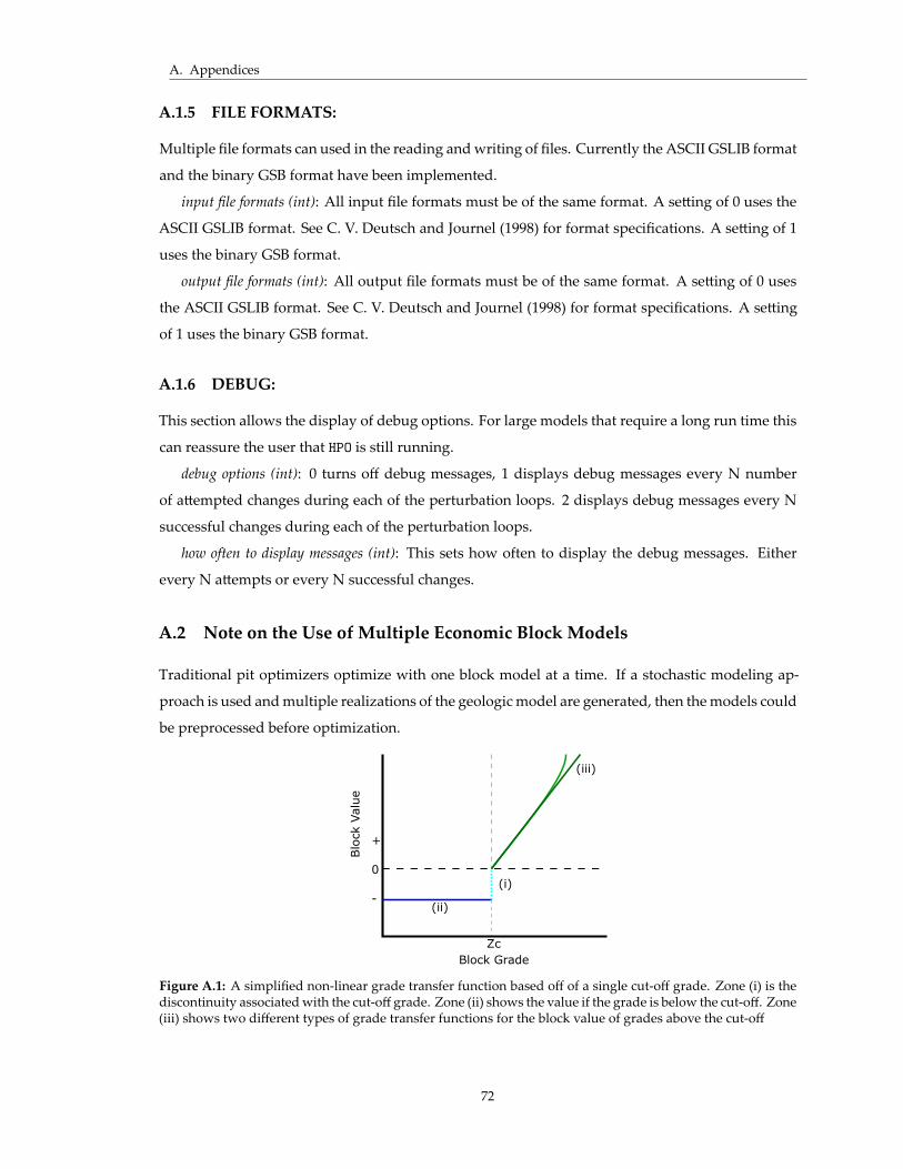
A. Appendices
A.1.5 FILE FORMATS:
Multiple file formats can used in the reading and writing of files. Currently the ASCII GSLIB format
and the binary GSB format have been implemented.
input file formats (int): All input file formats must be of the same format. A se ing of 0 uses the
ASCII GSLIB format. See C. V. Deutsch and Journel (1998) for format specifications. A se ing of 1
uses the binary GSB format.
output file formats (int): All output file formats must be of the same format. A se ing of 0 uses
the ASCII GSLIB format. See C. V. Deutsch and Journel (1998) for format specifications. A se ing
of 1 uses the binary GSB format.
A.1.6 DEBUG:
This section allows the display of debug options. For large models that require a long run time this
can reassure the user that HPO is still running.
debug options (int): 0 turns off debug messages, 1 displays debug messages every N number
of a empted changes during each of the perturbation loops. 2 displays debug messages every N
successful changes during each of the perturbation loops.
how often to display messages (int): This sets how often to display the debug messages. Either
every N a empts or every N successful changes.
A.2 Note on the Use of Multiple Economic Block Models
Traditional pit optimizers optimize with one block model at a time. If a stochastic modeling ap-
proach is used and multiple realizations of the geologic model are generated, then the models could
be preprocessed before optimization.
Blo
ck V
alue
+
0
-
ZcBlock Grade
(i)
(ii)
(iii)
Figure A.1: A simplified non-linear grade transfer function based off of a single cut-off grade. Zone (i) is thediscontinuity associated with the cut-off grade. Zone (ii) shows the value if the grade is below the cut-off. Zone(iii) shows two different types of grade transfer functions for the block value of grades above the cut-off
72
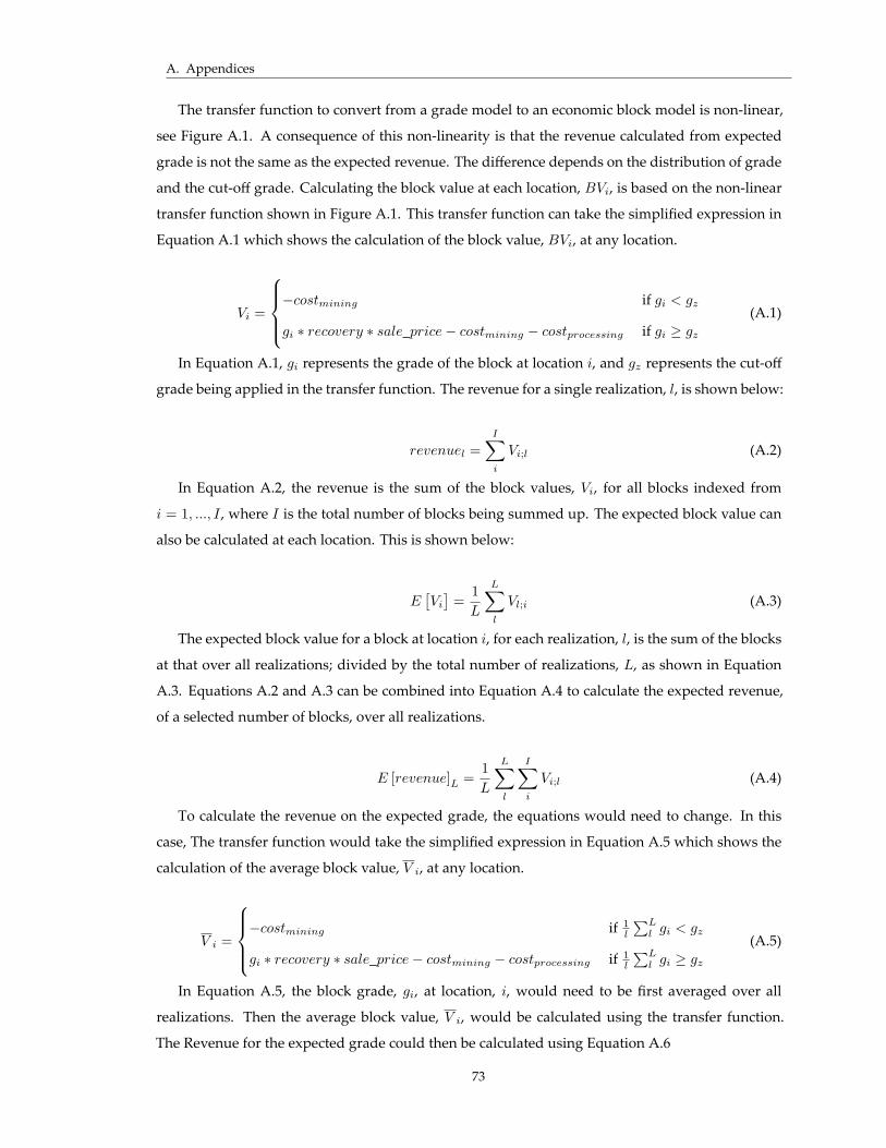
A. Appendices
The transfer function to convert from a grade model to an economic block model is non-linear,
see Figure A.1. A consequence of this non-linearity is that the revenue calculated from expected
grade is not the same as the expected revenue. The difference depends on the distribution of grade
and the cut-off grade. Calculating the block value at each location, BVi, is based on the non-linear
transfer function shown in Figure A.1. This transfer function can take the simplified expression in
Equation A.1 which shows the calculation of the block value, BVi, at any location.
Vi =
−costmining if gi < gz
gi ∗ recovery ∗ sale_price− costmining − costprocessing if gi ≥ gz
(A.1)
In Equation A.1, gi represents the grade of the block at location i, and gz represents the cut-off
grade being applied in the transfer function. The revenue for a single realization, l, is shown below:
revenuel =I∑i
Vi;l (A.2)
In Equation A.2, the revenue is the sum of the block values, Vi, for all blocks indexed from
i = 1, ..., I , where I is the total number of blocks being summed up. The expected block value can
also be calculated at each location. This is shown below:
E[Vi
]= 1
L
L∑l
Vl;i (A.3)
The expected block value for a block at location i, for each realization, l, is the sum of the blocks
at that over all realizations; divided by the total number of realizations, L, as shown in Equation
A.3. Equations A.2 and A.3 can be combined into Equation A.4 to calculate the expected revenue,
of a selected number of blocks, over all realizations.
E [revenue]L = 1L
L∑l
I∑i
Vi;l (A.4)
To calculate the revenue on the expected grade, the equations would need to change. In this
case, The transfer function would take the simplified expression in Equation A.5 which shows the
calculation of the average block value, V i, at any location.
V i =
−costmining if 1
l
∑Ll gi < gz
gi ∗ recovery ∗ sale_price− costmining − costprocessing if 1l
∑Ll gi ≥ gz
(A.5)
In Equation A.5, the block grade, gi, at location, i, would need to be first averaged over all
realizations. Then the average block value, V i, would be calculated using the transfer function.
The Revenue for the expected grade could then be calculated using Equation A.6
73
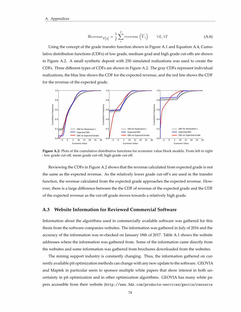
A. Appendices
RevenueE[g] =1I
I∑i
revenue(V i
)∀L,∀I (A.6)
Using the concept of the grade transfer function shown in Figure A.1 and Equation A.4, Cumu-
lative distribution functions (CDFs) of low grade, medium grad and high grade cut-offs are shown
in Figure A.2. A small synthetic deposit with 250 simulated realizations was used to create the
CDFs. Three different types of CDFs are shown in Figure A.2. The gray CDFs represent individual
realizations, the blue line shows the CDF for the expected revenue, and the red line shows the CDF
for the revenue of the expected grade.
5 0 5 10 15 20 25 30Economic Value
0.0
0.2
0.4
0.6
0.8
1.0
Cum
ulat
ive
Freq
uenc
y
EBV for Realization L Expected EBVEBV on Expected Grade
5 0 5 10 15 20 25 30Economic Value
0.0
0.2
0.4
0.6
0.8
1.0
Cum
ulat
ive
Freq
uenc
y
EBV for Realization L Expected EBVEBV on Expected Grade
5 0 5 10 15 20 25 30Economic Value
0.0
0.2
0.4
0.6
0.8
1.0
Cum
ulat
ive
Freq
uenc
y
EBV for Realization L Expected EBVEBV on Expected Grade
Figure A.2: Plots of the cumulative distributive functions for economic value block models. From left to right- low grade cut-off, mean grade cut-off, high grade cut-off.
Reviewing the CDFs in Figure A.2 shows that the revenue calculated from expected grade is not
the same as the expected revenue. As the relatively lower grade cut-off’s are used in the transfer
function, the revenue calculated from the expected grade approaches the expected revenue. How-
ever, there is a large difference between the the CDF of revenue of the expected grade and the CDF
of the expected revenue as the cut-off grade moves towards a relatively high grade.
A.3 Website Information for Reviewed Commercial Software
Information about the algorithms used in commercially available software was gathered for this
thesis from the software companies websites. The information was gathered in July of 2016 and the
accuracy of the information was re-checked on January 18th of 2017. Table A.1 shows the website
addresses where the information was gathered from. Some of the information came directly from
the websites and some information was gathered from brochures downloaded from the websites.
The mining support industry is constantly changing. Thus, the information gathered on cur-
rently available pit optimization methods can change with any new update to the software. GEOVIA
and Maptek in particular seem to sponsor multiple white papers that show interest in both un-
certainty in pit optimization and in other optimization algorithms. GEOVIA has many white pa-
pers accessible from their website (http://www.3ds.com/products-services/geovia/resource
74
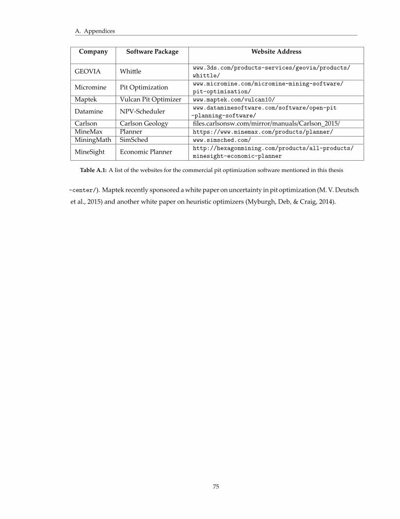
A. Appendices
Company Software Package Website Address
GEOVIA Whi le www.3ds.com/products-services/geovia/products/whittle/
Micromine Pit Optimization www.micromine.com/micromine-mining-software/pit-optimisation/
Maptek Vulcan Pit Optimizer www.maptek.com/vulcan10/
Datamine NPV-Scheduler www.dataminesoftware.com/software/open-pit-planning-software/
Carlson Carlson Geology files.carlsonsw.com/mirror/manuals/Carlson_2015/MineMax Planner https://www.minemax.com/products/planner/MiningMath SimSched www.simsched.com/
MineSight Economic Planner http://hexagonmining.com/products/all-products/minesight-economic-planner
Table A.1: A list of the websites for the commercial pit optimization software mentioned in this thesis
-center/). Maptek recently sponsored a white paper on uncertainty in pit optimization (M. V. Deutsch
et al., 2015) and another white paper on heuristic optimizers (Myburgh, Deb, & Craig, 2014).
75