Pitch Tracking - Boersma

7/28/2019 Pitch Tracking - Boersma

http://slidepdf.com/reader/full/pitch-tracking-boersma 1/14

IFA Proceedings 17, 1993 97

Institute of Phonetic Sciences,University of Amsterdam,Proceedings 17 (1993), 97-110.

ACCURATE SHORT-TERM ANALYSISOF THE FUNDAMENTAL FREQUENCY

AND THE HARMONICS-TO-NOISE RATIOOF A SAMPLED SOUND

Paul Boersma

Abstract

We present a straightforward and robust algorithm for periodicity detection, working inthe lag (autocorrelation) domain. When it is tested for periodic signals and for signalswith additive noise or jitter, it proves to be several orders of magnitude more accuratethan the methods commonly used for speech analysis. This makes our method capable of measuring harmonics-to-noise ratios in the lag domain with an accuracy and reliabilitymuch greater than that of any of the usual frequency-domain methods.

By definition, the best candidate for the acoustic pitch period of a sound can be foundfrom the position of the maximum of the autocorrelation function of the sound, while

the degree of periodicity (the harmonics-to-noise ratio) of the sound can be foundfrom the relative height of this maximum.

However, sampling and windowing cause problems in accurately determining theposition and height of the maximum. These problems have led to inaccurate time-domain and cepstral methods for pitch detection, and to the exclusive use of frequency-domain methods for the determination of the harmonics-to-noise ratio.

In this paper, I will tackle these problems. Table 1 shows the specifications of theresulting algorithm for two spectrally maximally different kinds of periodic sounds: asine wave and a periodic pulse train; other periodic sounds give results between these.

Table 1. The accuracy of the algorithm for a sampled sine wave and for a correctlysampled periodic pulse train, as a function of the number of periods that fit in the

duration of a Hanning window. These results are valid for pitch frequencies up to 80% of the Nyquist frequency. These results were measured for a sampling frequency of 10 kHzand window lengths of 40 ms (for pitch) and 80 ms (for HNR), but generalize to othersampling frequencies and window lengths (see section 5).

Periods perwindow

Pitch determination error∆F / F

Resolution of determinationof harmonics-to-noise ratio

sine wave pulse train sine wave pulse train> 3 < 5·10–4 < 5·10–5 > 27 dB > 12 dB

> 6 < 3·10–5 < 5·10–6 > 40 dB > 29 dB

> 12 < 4·10–7 < 2·10–7 > 55 dB > 44 dB

> 24 < 2·10–8

< 2·10–8

> 72 dB > 58 dB



98 IFA Proceedings 17, 1993

1 Autocorrelation and periodicity

For a time signal x(t ) that is stationary (i.e., its statistics are constant), theautocorrelation r x(τ ) as a function of the lag τ is defined as

r x τ ( ) ≡ x t ( )∫ x t + τ ( )dt (1)

This function has a global maximum for τ = 0. If there are also global maxima outside0, the signal is called periodic and there exists a lag T 0, called the period , so that allthese maxima are placed at the lags nT 0, for every integer n, with r x(nT 0) = r x(0). The

fundamental frequency F 0 of this periodic signal is defined as F 0 = 1 T 0 . If there areno global maxima outside 0, there can still be local maxima. If the highest of these isat a lag τ max , and if its height r x(τ max) is large enough, the signal is said to have aperiodic part, and its harmonic strength R0 is a number between 0 and 1, equal to thelocal maximum ′r x (τ max ) of the normalized autocorrelation

′r x τ ( ) ≡r x τ ( )r x 0( )

(2)

We could make such a signal x(t ) by taking a periodic signal H (t ) with a period T 0 andadding a noise N (t ) to it. We can infer from equation (1) that if these two parts areuncorrelated, the autocorrelation of the total signal equals the sum of theautocorrelations of its parts. For zero lag, we have r x (0) = r H (0) + r N (0), and if thenoise is white (i.e., if it does not correlate with itself), we find a local maximum at alag τ max = T 0 with a height r x (τ max ) = r H (T 0 ) = r H (0). Because the autocorrelationof a signal at zero lag equals the power in the signal, the normalized autocorrelation atτ max represents the relative power of the periodic (or harmonic) component of the

signal, and its complement represents the relative power of the noise component:

′r x τ max( ) =r H 0( )

r x 0( ); 1 − ′r x τ max( ) =

r N 0( )

r x 0( )(3)

This allows us to define the logarithmic harmonics-to-noise ratio (HNR) as

HNR (in dB) = 10 ⋅10log′r x τ max( )

1− ′r x τ max( )(4)

This definition follows the same idea as the frequency-domain definitions used bymost other authors, but yields much more accurate results thanks to the precision withwhich we can estimate r x(τ ). For perfectly periodic sounds, the HNR is infinite.

For non-stationary (i.e., dynamically changing) signals, the short-termautocorrelation at a time t is estimated from a short windowed segment of the signalcentred around t . This gives estimates F 0(t ) for the local fundamental frequency and

R0(t ) for the local harmonic strength. If we want these estimates to have a meaning atall, they should be as close as possible to the quantities derived from equation (1), if we perform a short-term analysis on a stationary signal. Sections 2 and 3 show how tocope with the windowing and sampling problems that arise. Section 4 presents thecomplete algorithm. Sections 5, 6, and 7 investigate the performance of the algorithmfor three kinds of stationary signals: periodic signals without perturbations, with

additive noise, and with jitter.




2 Windowing and the lag domain

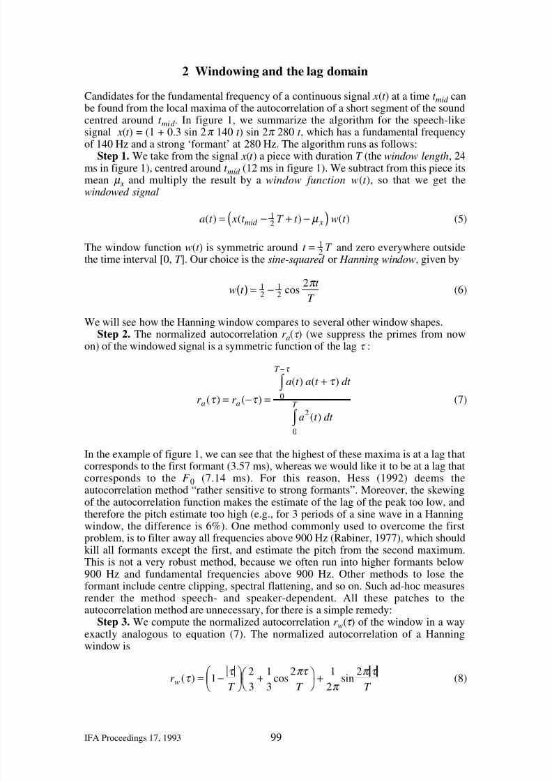
Candidates for the fundamental frequency of a continuous signal x(t ) at a time t mid canbe found from the local maxima of the autocorrelation of a short segment of the soundcentred around t mid . In figure 1, we summarize the algorithm for the speech-like

signal x(t ) = (1 + 0.3 sin 2π 140 t ) sin 2π 280 t , which has a fundamental frequencyof 140 Hz and a strong ‘formant’ at 280 Hz. The algorithm runs as follows:Step 1. We take from the signal x(t ) a piece with duration T (the window length, 24

ms in figure 1), centred around t mid (12 ms in figure 1). We subtract from this piece itsmean µ x and multiply the result by a window function w(t ), so that we get thewindowed signal

a(t ) = x(t mid −12

T + t ) − µ x( ) w(t ) (5)

The window function w(t ) is symmetric around t = 12

T and zero everywhere outsidethe time interval [0, T ]. Our choice is the sine-squared or Hanning window, given by

w t ( ) = 12

− 12

cos2π t

T (6)

We will see how the Hanning window compares to several other window shapes.Step 2. The normalized autocorrelation r a(τ ) (we suppress the primes from now

on) of the windowed signal is a symmetric function of the lag τ :

r a(τ ) = r a (−τ ) =

a(t )

0

T −τ

∫ a(t + τ ) dt

a2(t )

0

T

∫ dt

(7)

In the example of figure 1, we can see that the highest of these maxima is at a lag thatcorresponds to the first formant (3.57 ms), whereas we would like it to be at a lag thatcorresponds to the F 0 (7.14 ms). For this reason, Hess (1992) deems theautocorrelation method “rather sensitive to strong formants”. Moreover, the skewingof the autocorrelation function makes the estimate of the lag of the peak too low, andtherefore the pitch estimate too high (e.g., for 3 periods of a sine wave in a Hanningwindow, the difference is 6%). One method commonly used to overcome the firstproblem, is to filter away all frequencies above 900 Hz (Rabiner, 1977), which should

kill all formants except the first, and estimate the pitch from the second maximum.This is not a very robust method, because we often run into higher formants below900 Hz and fundamental frequencies above 900 Hz. Other methods to lose theformant include centre clipping, spectral flattening, and so on. Such ad-hoc measuresrender the method speech- and speaker-dependent. All these patches to theautocorrelation method are unnecessary, for there is a simple remedy:

Step 3. We compute the normalized autocorrelation r w(τ ) of the window in a wayexactly analogous to equation (7). The normalized autocorrelation of a Hanningwindow is

r w

(τ ) = 1−τ

T

2

3+

1

3cos

2πτ

T

+

1

2π sin

2π τ

T (8)



Time (ms) ->0 24-1

1

Time (ms) ->0 240

1

Time (ms) ->0 24-1

1

Lag (ms) ->0 7.14 24-1

1

Lag (ms) ->0 240

1

Lag (ms) ->0 7.14 24-1

1


x(t ) multiplied by w(t ) gives a(t )

r a(τ ) divided by r w(τ ) gives r x(τ )

Fig. 1. How to window a sound segment, and how to estimate the autocorrelation of a

sound segment from the autocorrelation of its windowed version. The estimatedautocorrelation r x(τ ) is not shown for lags longer than half the window length, because itbecomes less reliable there for signals with few periods per window.

To estimate the autocorrelation r x(τ ) of the original signal segment, we divide theautocorrelation r a(τ ) of the windowed signal by the autocorrelation r w(τ ) of thewindow:

r x (τ ) ≈ r a(τ )

r w (τ )(9)

This estimation can easily be seen to be exact for the constant signal x(t ) = 1 (withoutsubtracting the mean, of course); for periodic signals, it brings the autocorrelationpeaks very near to 1 (see figure 1). The need for this correction seems to have gone byunnoticed in the literature; e.g., Rabiner (1977) states that “no matter which windowis selected, the effect of the window is to taper the autocorrelation function smoothlyto 0 as the autocorrelation index increases”. With equation (9), this is no longer true.

The accuracy of the algorithm is determined by the reliability of the estimation (9),which depends directly on the shape of the window. For instance, for a periodic pulsetrain, which is defined as

x t ( ) = δ t − t 0 − nT 0( )n=−∞

+∞

∑ (10)

where T 0 is the period and t 0 / T (with 0 ≤ t 0 < T 0 ) represents the phase of the pulsetrain in the window, our estimate for the relevant peak of the autocorrelation is

r x T 0( ) =w t 0 + nT 0( ) w t 0 + n +1( )T 0( )

n

∑r w T 0( ) w

2t 0 + nT 0( )

n

∑(11)

This depends on the phase t 0 / T . If the window is symmetric and the pulse train is

symmetric around the middle of the window, the derivatives with respect to t 0 of both



Time ->

0

1

Time ->

0

1


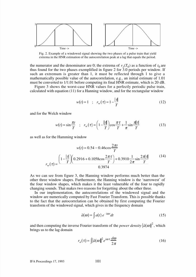
Fig. 2. Example of a windowed signal showing the two phases of a pulse train that yieldextrema in the HNR estimation of the autocorrelation peak at a lag that equals the period.

the numerator and the denominator are 0; the extrema of r x(T 0) as a function of t 0 arethus found for the two phases exemplified in figure 2 for 3.0 periods per window. If such an extremum is greater than 1, it must be reflected through 1 to give amathematically possible value of the autocorrelation, e.g., an initial estimate of 1.01must be converted to 1/1.01 before computing its final HNR estimate, which is 20 dB.

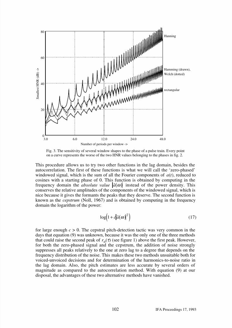
Figure 3 shows the worst-case HNR values for a perfectly periodic pulse train,calculated with equation (11) for a Hanning window, and for the rectangular window

w t ( ) = 1 ; r w τ ( ) = 1 −τ

T (12)

and for the Welch window

w t ( ) = sinπ t

T ; r w τ ( ) = 1 −

τ

T

cos

πτ

T +

1

π sin

π τ

T (13)

as well as for the Hamming window

w t ( ) = 0.54 − 0.46cos 2π t T

r w τ ( ) =1−

τ

T

0.2916 + 0.1058cos

2πτ

T

+ 0.3910

1

2π sin

2π τ

T

0.3974

(14)

As we can see from figure 3, the Hanning window performs much better than theother three window shapes. Furthermore, the Hanning window is the ‘narrowest’ of the four window shapes, which makes it the least vulnerable of the four to rapidlychanging sounds. That makes two reasons for forgetting about the other three.

In our implementation, the autocorrelations of the windowed signal and thewindow are numerically computed by Fast Fourier Transform. This is possible thanksto the fact that the autocorrelation can be obtained by first computing the Fouriertransform of the windowed signal, which gives in the frequency domain

a ω ( ) = a t ( )∫ e−iω t dt (15)

and then computing the inverse Fourier transform of the power density a ω ( )2

, whichbrings us to the lag domain

r a

τ ( )=

a ω ( )2eiω τ d ω

2π ∫ (16)



Hanning

Hamming (drawn),

Welch (dotted)

rectangular

0

20

40

60

80

S m a l l e s t H N R ( d B ) - >

3.0 6.0 12.0 24.0 48.0

Number of periods per window ->


Fig. 3. The sensitivity of several window shapes to the phase of a pulse train. Every pointon a curve represents the worse of the two HNR values belonging to the phases in fig. 2.

This procedure allows us to try two other functions in the lag domain, besides theautocorrelation. The first of these functions is what we will call the ‘zero-phased’windowed signal, which is the sum of all the Fourier components of a(t ), reduced tocosines with a starting phase of 0. This function is obtained by computing in thefrequency domain the absolute value a ω ( ) instead of the power density. Thisconserves the relative amplitudes of the components of the windowed signal, which isnice because it gives the formants the peaks that they deserve. The second function isknown as the cepstrum (Noll, 1967) and is obtained by computing in the frequencydomain the logarithm of the power:

log 1 + c a ω ( )2( ) (17)

for large enough c > 0. The cepstral pitch-detection tactic was very common in thedays that equation (9) was unknown, because it was the only one of the three methodsthat could raise the second peak of r a(τ ) (see figure 1) above the first peak. However,for both the zero-phased signal and the cepstrum, the addition of noise stronglysuppresses all peaks relatively to the one at zero lag to a degree that depends on thefrequency distribution of the noise. This makes these two methods unsuitable both forvoiced-unvoiced decisions and for determination of the harmonics-to-noise ratio inthe lag domain. Also, the pitch estimates are less accurate by several orders of magnitude as compared to the autocorrelation method. With equation (9) at ourdisposal, the advantages of these two alternative methods have vanished.




3 Sampling and the lag domain

Consider a continuous time signal x(t ) that contains no frequencies above a certainfrequency f max. We can sample this signal at regular intervals ∆t ≤ 1 (2 f max ) so thatwe know only the values xn at equally spaced times t n:

xn = x t n( ) ; t n = t 0 + n∆t (18)

We lose no data in this sampling, because we can reconstruct the original signal as

x(t ) = xn

sin π t − t n( ) / ∆t

π t − t n( ) / ∆t n=−∞

+∞

∑ (19)

The autocorrelation computed from the sampled signal is also a sampled function:

r n = r n∆τ ( )

There is a local maximum in the autocorrelation between (m–1)∆τ and (m+1)∆τ if

r m > r m−1 and r m > r m+1 (20)

A first crude estimate of the pitch period would be τ max ≈ m ∆τ , but this is not veryaccurate: with a sampling frequency of 10 kHz and ∆τ = ∆t , the pitch resolution forfundamental frequencies near 300 Hz is 9 Hz (which is the case for most time-domainpitch-detection algorithms); moreover, the height of the autocorrelation peak (r m) canbe as low as 2/ π = 0.636 for correctly sampled pulse trains (i.e., filtered with a phase-

preserving low-pass filter at the Nyquist frequency prior to sampling), which rendersHNR determination impossible and introduces octave errors in the determination of the fundamental period. We can improve this by parabolic interpolation around m∆τ :

τ max ≈ ∆τ m +12

r m+1 − r m−1( )2r m − r m−1 − r m+1

; r max ≈ r m +r m+1 − r m−1( )

2

8 2r m − r m−1 − r m+1( )(21)

However, though the error in the estimated period reduces to less than 0.1 sample, theheight of the relevant autocorrelation peak can still be as low as 7/(3π) = 0.743.

Now for the solution. We should use a ‘sin x / x’ interpolation, like the one inequation (19), in the lag domain (we do a simple upsampling in the frequency

domain, so that ∆τ = ∆t /2). As we cannot do the infinite sum, we interpolate over afinite number of samples N to the left and to the right, using a Hanning window againto taper the interpolation to zero at the edges:

r (τ ) ≈ r nr −n

sin π ϕ l + n −1( )π ϕ l + n −1( )n=1

N

∑ 12

+ 12

cosπ ϕ l + n − 1( )

ϕ l + N

+

r nl +n

sin π ϕ r + n −1( )π ϕ r + n − 1( )n=1

N

∑ 12

+ 12

cosπ ϕ r + n −1( )

ϕ r + N

(22)

where nl ≡ largest integer ≤ τ

∆τ

; nr ≡ nl + 1 ; ϕ l ≡τ

∆τ

− nl ; ϕ r ≡ 1− ϕ l




In our implementation, N is the smaller of 500 and the largest number for which(nl + N )∆τ is smaller than half the window length. This is because the estimation of the autocorrelation is not reliable for lags greater than half the window length, if thereare few periods per window (see figure 1). Note that the interpolation can involveautocorrelation values for negative lags.

The places and heights of the maxima of equation (22) can be determined withgreat precision (they are looked for between (m–1)∆τ and (m+1)∆τ ). We can showthis with long windows, where the windowing effects have gone, but the samplingeffects remain. E.g., with a 40-ms window, any signal with a frequency of exactly3777 Hz, sampled at 10 kHz, will be consistently measured as having a fundamentalfrequency of 3777.00000 ± 0.00001 Hz (accuracy 10–8 sample in the lag domain,

N =394) and a first autocorrelation peak between 0.99999999 and 1. The measuredHNR (80-ms window) is 94.0 ± 0.1 dB. This looks like a real improvement.

4 Algorithm

A summary of the complete 9-parameter algorithm, as it is implemented into thespeech analysis and synthesis program praat , is given here:

Step 1. Preprocessing: to remove the sidelobe of the Fourier transform of theHanning window for signal components near the Nyquist frequency, we perform asoft upsampling as follows: do an FFT on the whole signal; filter by multiplication inthe frequency domain linearly to zero from 95% of the Nyquist frequency to 100% of the Nyquist frequency; do an inverse FFT of order one higher than the first FFT.

Step 2. Compute the global absolute peak value of the signal (see step 3.3).Step 3. Because our method is a short-term analysis method, the analysis is

performed for a number of small segments ( frames) that are taken from the signal insteps given by the TimeStep parameter (default is 0.01 seconds). For every frame, we

look for at most MaximumNumberOfCandidatesPerFrame (default is 4) lag-heightpairs that are good candidates for the periodicity of this frame. This number includesthe unvoiced candidate, which is always present. The following steps are taken foreach frame:

Step 3.1. Take a segment from the signal. The length of this segment (the windowlength) is determined by the MinimumPitch parameter, which stands for the lowestfundamental frequency that you want to detect. The window should be just longenough to contain three periods (for pitch detection) or six periods (for HNRmeasurements) of MinimumPitch. E.g. if MinimumPitch is 75 Hz, the window lengthis 40 ms for pitch detection and 80 ms for HNR measurements.

Step 3.2. Subtract the local average.Step 3.3. The first candidate is the unvoiced candidate, which is always present.

The strength of this candidate is computed with two soft threshold parameters. E.g., if VoicingThreshold is 0.4 and SilenceThreshold is 0.05, this frame bears a good chanceof being analyzed as voiceless (in step 4) if there are no autocorrelation peaks aboveapproximately 0.4 or if the local absolute peak value is less than approximately 0.05times the global absolute peak value, which was computed in step 2.

Step 3.4. Multiply by the window function (equation 5).Step 3.5. Append half a window length of zeroes (because we need autocorrelation

values up to half a window length for interpolation).Step 3.6. Append zeroes until the number of samples is a power of two.Step 3.7. Perform a Fast Fourier Transform (discrete version of equation 15), e.g.,

with the algorithm realft from Press et al. (1989).

Step 3.8. Square the samples in the frequency domain.




Step 3.9. Perform a Fast Fourier Transform (discrete version of equation 16). Thisgives a sampled version of r a(τ ).

Step 3.10. Divide by the autocorrelation of the window, which was computed oncewith steps 3.5 through 3.9 (equation 9). This gives a sampled version of r x(τ ).

Step 3.11. Find the places and heights of the maxima of the continuous version of

r x(τ ), which is given by equation 22, e.g., with the algorithmbrent

from Press et al.(1989). The only places considered for the maxima are those that yield a pitchbetween MinimumPitch and MaximumPitch. The MaximumPitch parameter should bebetween MinimumPitch and the Nyquist frequency. The only candidates that areremembered, are the unvoiced candidate, which has a local strength equal to

R ≡ VoicingThreshold + max 0, 2 −local absolute peak ( ) global absolute peak ( )

SilenceThreshold 1 + VoicingThreshold ( )

(23)

and the voiced candidates with the highest ( MaximumNumberOfCandidatesPerFrameminus 1) values of the local strength

R ≡ r τ max( ) − OctaveCost ⋅ 2log MinimumPitch ⋅ τ max( ) (24)

The OctaveCost parameter favours higher fundamental frequencies. One of thereasons for the existence of this parameter is that for a perfectly periodic signal all thepeaks are equally high and we should choose the one with the lowest lag. Otherreasons for this parameter are unwanted local downward octave jumps caused byadditive noise (section 6). Finally, an important use of this parameter lies in thedifference between the acoustic fundamental frequency and the perceived pitch. Forinstance, the harmonically amplitude-modulated signal with modulation depth d mod

x t ( ) = 1 + d mod sin2π Ft ( ) sin 4π Ft (25)

has an acoustic fundamental frequency of F , whereas its perceived pitch is 2F formodulation depths smaller than 20 or 30 percent. Figure 1 shows such a signal, with amodulation depth of 30%. If we want the algorithm’s criterion to be at 20% (in orderto fit pitch perception), we should set the OctaveCost parameter to (0.2)2 = 0.04; if wewant it to be low (in order to detect vocal-fold periodicity), say 5%, we should set itto (0.05)2 = 0.0025. The default value is 0.01, corresponding to a criterion of 10%.

After performing step 2 for every frame, we are left with a number of frequency-strength pairs (F ni, Rni), where the index n runs from 1 to the number of frames, and iis between 1 and the number of candidates in each frame. The locally best candidate

in each frame is the one with the highest R. But as we can have several approximatelyequally strong candidates in any frame, we can launch on these pairs the global path

finder , the aim of which is to minimize the number of incidental voiced-unvoiceddecisions and large frequency jumps:

Step 4. For every frame n, pn is a number between 1 and the number of candidatesfor that frame. The values { pn | 1 ≤ n ≤ number of frames} define a path through thecandidates: {(F npn

, Rnpn) | 1 ≤ n ≤ number of frames}. With every possible path we

associate a cost

cost pn{ }( ) = transitionCost F n−1, pn−1,F npn

( )n=2

numberOfFrames

∑ − Rnpn

n=1

numberOfFrames

∑ (26)



Time (seconds) ->0 0.01-1

1

Time (seconds) ->0 0.01-1

1

Frequency (Hz) ->

S p e c t r u m ( d

B ) - >

0 5000-20

0

20

40

60

80

Frequency (Hz) ->

S p e c t r u m ( d

B ) - >

0 5000-20

0

20

40

60

80


where the transitionCost function is defined by (F = 0 means unvoiced)

transitionCost F 1, F 2( ) =

0 if F 1 = 0 and F 2 = 0

VoicedUnvoicedCost if F 1 = 0 xor F 2 = 0

OctaveJumpCost ⋅ 2logF 1

F 2if F 1 ≠ 0 and F 2 ≠ 0

(27)

where the VoicedUnvoicedCost and OctaveJumpCost parameters could both be 0.2.The globally best path is the path with the lowest cost. This path might contain somecandidates that are locally second-choice. We can find the cheapest path with the aidof dynamic programming, e.g., using the Viterbi algorithm described for HiddenMarkov Models by Van Alphen & Van Bergem (1989).

For stationary signals, the global path finder can easily remove all local octaveerrors, even if they comprise as many as 40% of all the locally best candidates(section 6 presents an example). This is because the correct candidates will be almostas strong as the incorrectly chosen candidates. For most dynamically changingsignals, the global path finder can still cope easily with 10% local octave errors.

For many measurements in this article, we turn the path finder off by setting theVoicedUnvoicedCost and OctaveJumpCost parameters to zero; in this way, thealgorithm selects the locally best candidate for each frame.

For HNR measurements, the path finder is turned off, and the OctaveCost andVoicingThreshold parameters are zero, too; MaximumPitch equals the Nyquistfrequency; only the TimeStep, MinimumPitch, and SilenceThreshold parameters arerelevant for HNR measurements.

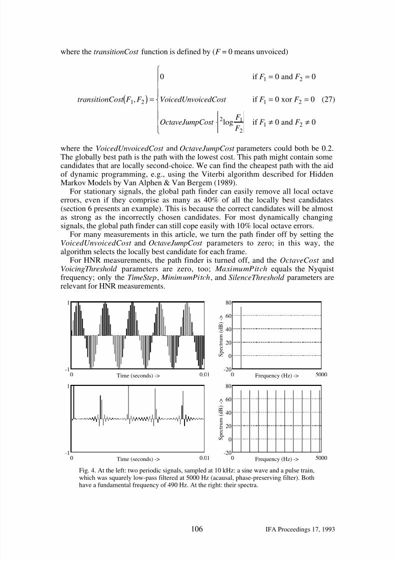
Fig. 4. At the left: two periodic signals, sampled at 10 kHz: a sine wave and a pulse train,which was squarely low-pass filtered at 5000 Hz (acausal, phase-preserving filter). Bothhave a fundamental frequency of 490 Hz. At the right: their spectra.




5 Accuracy in measuring perfectly periodic signals

The formula for a sampled perfect sine wave with frequency F is

xn = sin 2π Ft n (28)

and the formula for a correctly sampled pulse train (squarely low-pass filtered at theNyquist frequency) with period T is

xn =sin π F s t n − mT ( )

π F s t n − mT ( )m=−∞

+∞

∑ (29)

These two functions form spectrally maximally different periodic signals. Figure 4shows examples of these signals, together with their spectra. The spectrum of the sinewave is maximally narrow, that of the pulse train is maximally wide.

Table 1 (page 97) shows our algorithm’s accuracy in determining pitch and HNR.

We see from table 1 that for pitch detection there should be at least three periods in awindow. The value of 27 dB appearing in table 1 for a sine wave with the worst phase(symmetric in window) and the worst period (one third of a window), means that theautocorrelation peak can be as low as 0.995, which means that the signal

xn = 1 + d mod sin2π Ft n( ) sin 4π Ft n (30)

(see also figure 1), whose fundamental frequency is F , can be locally ambiguous for F near MinimumPitch, if the modulation depth d mod is less than √ 1–0.995 = 7%. Thecritical modulation depth, at which there are 10% local octave errors (detection of 2F as the best candidate), is 5%, for the lowest F (equal to MinimumPitch). Note that the

global path finder will not have any trouble removing these octave errors.We also see from table 1 that for HNR measurements, there should be at least 6.0

periods per window. The values measured for the HNR of a pulse train are the sameas those predicted by theory for continuous signals, as plotted in figure 3. Thissuggests that the windowing effects have the larger part of the influence on HNRmeasurement inaccuracy, and that the sampling effects have been effectivelycancelled by equation (22).

For very short windows (less than 20 samples in the time domain, MinimumPitchgreater than 30% of the Nyquist frequency), the HNR values for pulse trains do notdeteriorate, but those for sine waves approach the values for pulse trains; the relativepitch determination error rises to 10-4.

The problems with short-term HNR measurements in the frequency domain, arethe sidelobes of the harmonics and the sidelobes of the Fourier transform of thewindow: they occur throughout the spectrum. Pitch-synchronous algorithms try tocope with the first problem, but they require prior accurate knowledge of the period(Cox et al., 1989; Yumoto et al., 1982). Using fixed window lengths in the frequencydomain requires windows to be long: the shortest window used by Klingholz (1987)spans 12 periods, De Krom (1993) needs 8.2 periods; with the shortest window, bothhave a HNR resolution of apx. 30 dB for synthetic vowels, as opposed to our 37 dBwith only 6 periods (48 dB for 8.2 periods, 52 dB for 12 periods). In theautocorrelation domain, the only sidelobe that could stir trouble, is the one that causesaliasing for frequency components near the Nyquist frequency; that one is easilyfiltered out. This is the cause of the superior results with the present method.



m e a s u r e H

N R ( B ) - >

SNR (dB) ->-30 -20 -10 0 10 20 30 40 50

-10

0

10

20

30

40

50

60

-30 -20 -10 0 10 20 30 40 50 60-10

0

10

20

30

40

50

60

SNR (dB) ->

m e a s u r e d H N R ( d B ) - >


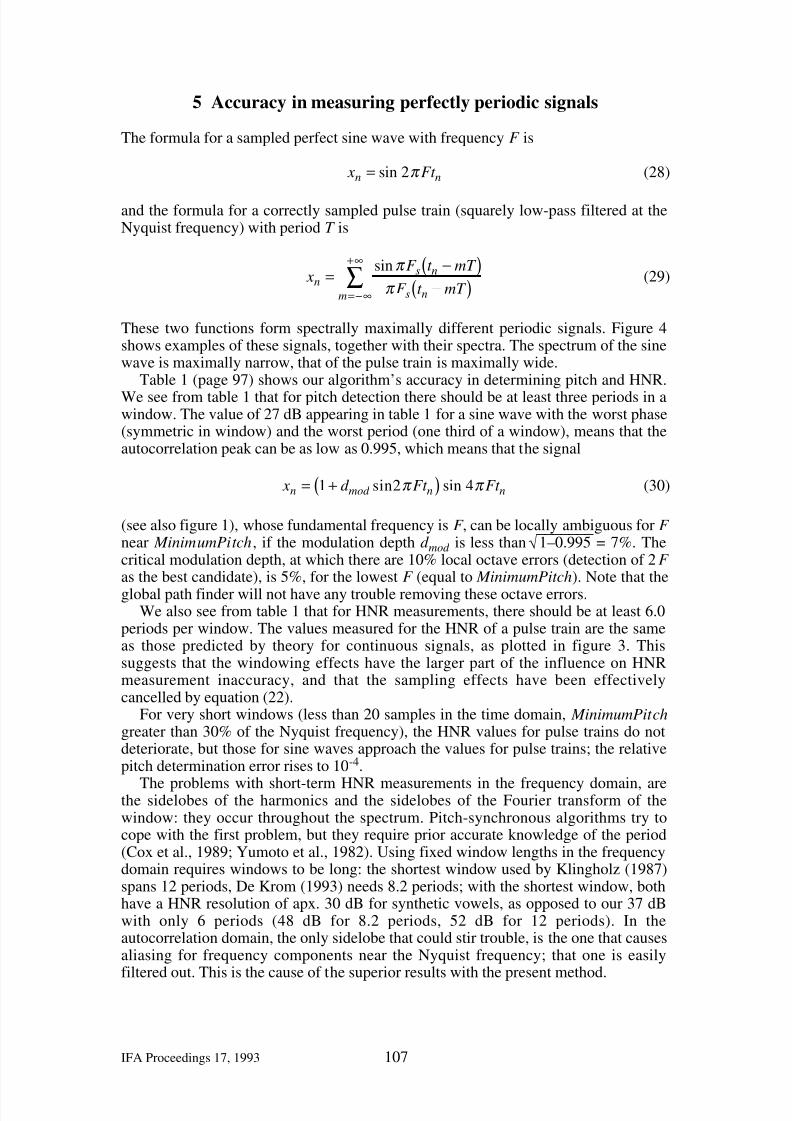
Fig. 5. Measured HNR values for a sine wave (left) and a pulse train (right) sampled at

10 kHz, both with a periodicity of 103 Hz, with additive noise. The figures show the10%, median, and 90% curves. The window length was 80 ms.

6 Sensitivity to additive noise

The formula for a sampled sound consisting of a sine wave with frequency F andadditive ‘white’ noise (squarely low-pass filtered at the Nyquist frequency) is

xn = 2 sin2π Ft n + 10−SNR /20 zn (31)

where SNR is the signal-to-noise ratio, expressed in dB, and zn is a sequence of real

numbers that are independently drawn from a Gaussian distribution with zero meanand unit variance. The formula for a sampled sound consisting of a correctly sampledpulse train (squarely low-pass filtered at the Nyquist frequency) with period T andadditive ‘white’ noise is

xn =F s / F

1− F / F s

sin π F s t n − mT ( )π F s t n − mT ( )m=−∞

+∞

∑ +10−SNR /20 zn (32)

Adding noise obscures the underlying fundamental frequency. For example,additive noise with a SNR of 20 dB gives the following results for sounds with anunderlying F 0 of 103 Hz, sampled at 10 kHz, and analyzed with a MinimumPitch of

75 Hz (40-ms window): the relative pitch ‘error’ (measured as the worse of the 10%and 90% points of the distribution of the measured pitch) rises to 0.7% for a sinewave, and to 0.007% for a pulse train (these ‘errors’ are not failures of the algorithm:they are signal properties). Gross pitch determination ‘errors’ (more than 10% off) areonly found for negative signal-to-noise ratios (more noise than signal).

For a sine wave with a frequency of 206 Hz and a window length of 40 ms( MinimumPitch is 75 Hz), with noise added at a SNR of 20 dB, there are 40% localoctave ‘errors’ (a detected pitch of 103 Hz; these are not failures of the algorithm,either: the 103 Hz is locally in the signal) if the OctaveCost parameter is 0.001. Theglobal path finder leaves 0% octave ‘errors’. However, we cannot expect this goodbehaviour for dynamically changing signals. There remain 10% local octave ‘errors’

if the OctaveCost parameter is raised to 0.003. This gives a critical modulation depthof √ 0.003 = 5%. Thus, if we want to detect reliably the pitch of noisy signals, we



jitter depth (dB) ->

m e a s u r e d H N R

( d B ) - >

-10 -20 -30 -40 -50 -60 -70 -80-10

0

10

20

30

40

50

60

70

jitter depth (dB) ->

m e a s u r e d H N R

( d B ) - >

-10 -20 -30 -40 -50 -60 -70 -80-10

0

10

20

30

40

50

60

70


Fig. 6. Measured HNR values for a sine wave (left) and a pulse train (right), sampled at10 kHz, with fundamental frequencies that vary randomly around 103 Hz. The curves areshown for window lengths of 60, 80, 150, and 600 milliseconds. The short windows giveslightly larger HNR values than the long windows, except where the HNR measurementsfor short windows level off for very low jitter depths.

should not expect to see the difference between the fundamental frequency and a firstformant whose relative amplitude is higher than 95% (we must note here that thezero-phased signal would raise this number to 97%).

We see from figure 5 that the measured HNR values are within a few dB from theunderlying SNR values (between 0 and 40 dB). These results are better than thosefound in the literature so far. For instance, in De Krom (1993), the measured HNRvalues for additive noise depend to a large degree on the number of periods per

window: for a SNR of 40 dB (in the glottal source, before a linear filter), the averagedHNR varies from 27 dB for 8.2 periods per window (102.4 ms / 80 Hz) to 46 dB for121 periods per window (409.6 ms / 296 Hz), and the slope of HNR as a function of SNR is 0.7. With our algorithm, the median HNR, for a SNR of 40 dB, varies from39.0 dB for 8.2 periods per window (103 Hz / 80 ms) to 40.0 dB for large windows,and the slope is near to the theoretical value of 1.

7 Sensitivity to random frequency modulations (jitter)

A jittered pulse train with average period T av has its events at the times

T n = T n−1 + T av 1 + jitterDepth ⋅ zn( ) (33)

A jittered sine wave with average frequency F av involves a randomly walking phase:

xn = sin 2π F avn∆t + ϕ n( ) ; ϕ n = ϕ n−1 + 2π ⋅ jitterDepth ⋅ F av∆t ⋅ zn (34)

For sine waves, the harmonics-to-noise ratio is much less sensitive to jitterDepth thanfor pulse trains. This is shown in figure 6 (jitter depth in dB is 20·10log jitterDepth).The slope of the HNR as a function of the logarithmic jitter depth is apx. –0.95, whichis closer to the theoretical value of 1 than De Krom’s (1993) value of –0.66.




8 Conclusion

Our measurements of the places and the heights of the peaks in the lag domain areseveral orders of magnitude more accurate than those of the usual pitch-detectionalgorithms. Due to its complete lack of local decision moments, the algorithm is very

straightforward, flexible and robust: it works equally well for low pitches (theauthor’s creaky voice at 16 Hz, alveolar trill at 23.4 Hz, and bilabial trill at 26.0 Hz),middle pitches (female speaker at 200 Hz), and high pitches (soprano at 1200 Hz, atwo-year-old child yelling [i] at 1800 Hz). The only ‘new’ tricks are twomathematically justified tactics: the division by the autocorrelation of the window(equation 9), and the ‘sin x / x’ interpolation in the lag domain (equation 22).

In measuring harmonics-to-noise ratios, the present algorithm is not only muchsimpler, but also much more accurate, more reproducible, less dependent on periodand window length, and more resistant to rapidly changing sounds, compared to otheralgorithms found in the literature.

Postscript

After finishing this article, we discovered that the ‘Gaussian’ window, which is zerooutside the interval − 1

2T , 3

2T [ ], and (exp(−12(t T − 1

2)2 ) − e

−12 ) (1− e−12 ) inside,

produces much better results than the Hanning window defined on [0,T ], though itseffective length is approximately the same. The worst pitch determination error (table1) falls from 5·10-4 to 10-6; the worst measurable HNR for a pulse train (at 6 effectiveperiods per window) rises from 29 dB to 58 dB, and for a sine wave it rises from 40to 75 dB. In figure 3, the theoretical value for a real Gaussian window at 6 effectiveperiods per window would be 58 dB (30 dB at 4.5 periods per window, and 170 dB at10 periods per window). In figures 5 and 6, the curves would not level off at 45 dB,

but at 60 and 80 dB instead. In practice, a window only 4.5 periods long guarantees aminimum HNR of 37 dB for vowel-like periodic signals (65 dB for 6 periods). Thismeans that we can improve again on the analysis of running speech.

References

Alphen, P. van, & Bergem, D.R. van (1989): “Markov models and their application in speechrecognition”, Proceedings of the Institute of Phonetic Sciences of the University of Amsterdam13: 1-26.

Cox, N.B., Ito, N.R., & Morrison, M.D. (1989): “Technical considerations in computation of spectralharmonics-to-noise ratios for sustained vowels”, J. Speech and Hearing Research 32: 203-218.

Hess, W.J. (1992): “Pitch and voicing determination”, in S. Furui & M.M. Sondhi (eds.): Advances inSpeech Signal Processing, Marcel Dekker, New York, pp. 3-48.

Klingholz, F. (1987): “The measurement of the signal-to-noise ratio (SNR) in continuous speech”,Speech Communication 6: 15-26.

Krom, G. de (1993): “A cepstrum-based technique for determining a harmonics-to-noise ratio inspeech signals”, Journal of Speech and Hearing Research 36: 254-265.

Noll, A.M. (1967): “Cepstrum pitch determination”, J. Acoust. Soc. America 41: 293-309.Press, W.H., Flannery, B.P., Teukolsky, S.A., & Vetterling, W.T. (1989): Numerical Recipes,

Cambridge University Press.Rabiner, L.R. (1977): “On the use of autocorrelation analysis for pitch detection”, IEEE Transactions

on Acoustics, Speech, and Signal Processing ASSP-25: 24-33.Yumoto, E., Gould, W.J., & Baer, T. (1982): “Harmonics-to-noise ratio as an index of the degree of

hoarseness”, Journal of the Acoustical Society of America 71: 1544-1550.

Documents

Pitch Tracking - Boersma