Place and Neighborhood Crime: Examining the Relationship between Schools, Churches, and

Alcohol Related Establishments and Crime

Prepared by:

Dale Willits Lisa Broidy

Ashley Gonzales Kristine Denman

New Mexico Statistical Analysis Center Dr. Lisa Broidy, Director

March 2011

1

TABLE OF CONTENTS

TABLE OF CONTENTS .................................................................................................... 1 

LIST OF TABLES .............................................................................................................. 2 

CHAPTER I: INTRODUCTION ........................................................................................ 3 

CHAPTER II: LITERATURE REVIEW ........................................................................... 5 

Routine Activity Theory ................................................................................................. 5 Social Disorganization Theory ....................................................................................... 6 Schools and Neighborhood Crime .................................................................................. 7 Churches and Neighborhood Crime ................................................................................ 9 Alcohol Establishments and Neighborhood Crime ......................................................... 9 Data ............................................................................................................................... 12 Methods......................................................................................................................... 17 

CHAPTER IV: RESULTS ................................................................................................ 20 

Place and Violent Crime ........................................................................................... 21 Place and Property Crime ......................................................................................... 23 Place and Narcotics Crime ........................................................................................ 25 

CHAPTER V: DISCUSSION AND CONCLUSION ...................................................... 28 

REFERENCES ................................................................................................................. 34 

APPENDIX: ADDITIONAL REGRESSION RESULTS ............................................... 38 

2

LIST OF TABLES Table 3.1. Crime Incidents from 2000 to 2005 by Block Group .........................................13 Table 3.2. Principal Components Matrix of Census Variables Using Varimax Rotation ...15 Table 3.3. Descriptive Statistics for Independent Variables (n = 430 block groups) ..........16 Table 3.4. Moran's I Results .................................................................................................18 Table 4.1. Regression Results on Violent Crime ..................................................................22 Table 4.2. Regression Results on Property Crime ................................................................24 Table 4.3. Regression Results on Narcotics Incidents ..........................................................26 Table A1. Poisson Regression Results Using Homicide as the Dependent Variable ..........38 Table A2. Negative Binomial Regression Results Using Rape as the Dependent Variable 39 Table A3. Negative Binomial Regression Results Using Aggravated Assault as the Dependent Variable ..............................................................................................................40 Table A4. Negative Binomial Regression Results Using Robbery as the Dependent Variable .................................................................................................................................41 Table A5. Negative Binomial Regression Results Using Burglary as the Dependent Variable .................................................................................................................................42 Table A6. Negative Binomial Regression Results Using Larceny as the Dependent Variable .................................................................................................................................43 Table A7. Negative Binomial Regression Results Using Motor Vehicle Theft as the Dependent Variable ..............................................................................................................44 Table A8. Negative Binomial Regression Results Using Narcotics Incidents as the Dependent Variable ..............................................................................................................45 

3

CHAPTER I: INTRODUCTION The objective of this research is to determine the degree to which neighborhood crime patterns are influenced by the spatial distribution of three types of places: schools, alcohol establishments, and churches. A substantial body of research has examined the relationship between places and crime. Empirically, this research indicates that there is more crime at certain types of places than at others (Sherman, Gartin, and Buerger, 1989; Spelmen, 1995; Block and Block, 1995). The criminological literature also provides several potential theoretical explanations for these patterns. The routine activity perspective (Cohen and Felson, 1979) argues that crime occurs when motivated offenders converge with potential victims in unguarded areas. Places that promote this convergence are expected to have elevated crime rates, while places that prevent or reduce this convergence are expected to have lower crime rates. The social disorganization perspective (Shaw and McKay, 1942; Bursik, 1988; Krivo and Peterson, 1996) argues that communities with more collective efficacy (in the form of internal social networks and access to external resources and values) are likely to have less crime, while communities lacking in efficacy are likely to have more crime. Places that promote the formation of positive social ties and grant the community access to external resources are expected to reduce crime, while places that inhibit positive social ties and separate the community from external resources are likely to increase crime. Much of the literature on place and crime has focused on the influence of bars on neighborhood crime rates, with a substantial body of research indicating that bars are associated with elevated crime rates (Roncek and Bell, 1981; Roncek and Pravatiner, 1989; Sherman, Gartin, and Buerger, 1989; Roncek and Maier, 1991; Block and Block, 1995). Sherman, Gartin, and Buerger (1989), for example, found that bars can account for upwards of 50% of police service calls in a given area. Here we examine the relationship not only between bars and crime rates, but other types of liquor establishments as well (e.g., liquor stores and restaurants that serve alcohol). In addition to the literature that characterizes bars as hot spots for crime, a smaller, yet growing, body of literature indicates that the presence of schools (Roncek and Lobosco, 1983; Roncek and Faggiani, 1985; Roman, 2004; Kautt and Roncek, 2007, Broidy, Willits, and Denman, 2009, Murray and Swatt, 2010) is also associated with neighborhood crime. The most recent of this research suggests that while high schools are associated with increased crime at the neighborhood level, elementary schools may have a protective influence. Research on churches and crime is limited relative to research focused on schools and bars, but suggests that churches may help protect neighborhoods from crime (Lee, 2006; Lee 2008; Lee 2010). Furthermore, there are theoretical reasons to suspect that churches, like schools and liquor establishments, may be an important type of place to consider when examining crime at the neighborhood level. The current research contributes to a criminological understanding of place and crime by examining whether and how all three location types operate to influence crime rates both independently and relative to one another.

4

Additionally, the current research controls for known neighborhood-level correlates of crime not often included in research examining place and crime. The place and crime research has generally been conducted at the smallest geographic unit defined by the U.S. Census Bureau: the block (for an exception, see Broidy, Willits, and Denman, 2009). The U.S. Census Bureau, however, releases data on a wider range of social indicators at larger levels of analysis (like the block group and tract). Consequently, previous research has been unable to control for a wide array of social-structural factors when examining the relationship between the distribution of places and the effect of this distribution on neighborhood crime. This leaves open the question of whether the relationship between place and crime is independent of factors such as structural disadvantage, residential mobility, and family disruption or simply a spurious reflection of these established relationships. In this study, using incident-crime data from Albuquerque, New Mexico, we assess the influence of place on neighborhood crime rates, net of key structural correlates of crime. We do this by utilizing the block group as our level of analysis. This allows us to investigate the effects of schools, liquor establishments and churches, while controlling for a wider array of variables than previous studies. By controlling for concepts like structural disadvantage, residential mobility, and family disruption, we can be more certain that any significant relationship between place and neighborhood crime is reflective of place effects and not of structural conditions. In sum, the current research examines the relationship between place and crime. We focus specifically on the relationship between schools, churches, and bars (including other alcohol establishments) and neighborhood crime. We focus particularly on the relative influence of different types of places on crime rates and on variations in the influence of place type by crime. In other words, do some place types have a more consistent influence on crime than others and does the strength of that influence depend on the type of crime we examine (e.g., violent v. property crime)? This report is divided into five chapters. The second chapter describes the theoretical framework utilized in this research and reviews the relevant literature on place and neighborhood crime. The third chapter describes the data and methodologies that we used to investigate the relationship between place and crime. The fourth chapter presents the results of our research. The final chapter discusses these results, presents empirical and theoretical conclusions, and addresses directions for policy and future research.

5

CHAPTER II: LITERATURE REVIEW Research examining the relationship between place and neighborhood crime is typically framed in terms of routine activities theory and social disorganization theory. In the following literature review we briefly describe each of these theoretical traditions. Then, we discuss how these theories might explain the relationship between specific types of places and neighborhood crime.

Routine Activity Theory Routine activity theory states that criminal acts require the convergence of three elements: motivated offenders, suitable targets, and the absence of capable guardianship (Cohen and Felson, 1979: 589). Building on utilitarian principles, the theory assumes that the absence of any one of these elements increases the risks of crime relative to its rewards, making crime less likely. At the macro-level, routine activity theory is rooted in the social and physical ecology perspective. According to this perspective, crime is “affected not only by the absolute size of the supply of offenders, targets, or guardianship, but also by the factors affecting the frequency of their convergence in space and time” (Sherman, Gartin, and Buerger, 1989: 30-31). In other words, specific places are likely to be crime prone because of associated routine activity patterns that are conducive to crime. A specific place may be criminogenic because it increases the prevalence of any combination of the three elements described by the routine activity perspective. The routine activity argument, when applied to types of places, focuses on the opportunity structures associated with specific places and how these shape the related probability that a criminal event occurs. Places that are frequented by motivated offenders are likely to exhibit a higher incidence rate of crime than others, as an increase in the number of would-be offenders present at a specific place increases the probability that these potential offenders will converge in time and space with suitable victims. Similarly, locations frequented by suitable victims are also expected to be more criminogenic than places that are avoided by suitable victims. Places where both potential offenders and potential victims converge in large numbers are expected to be especially criminogenic. Increases in the presence of would-be offenders and/or would-be victims are also expected to decrease the effectiveness of guardianship, as larger crowds skew the guardian-to-person ration, making it harder for would-be guardians to comprehensively monitor all of the people present in a given place. From this perspective, locations that promote the convergence of at-risk individuals or groups (that is, individuals or groups that can be generalized as “motivated offenders” or “suitable targets” because of their elevated levels of offending and victimization) are expected to be more criminogenic than others.

6

While Cohen and Felson (1979) did not address the issue of criminal motivation, other researchers employing the routine activities perspective have also argued that places can increase both the motivation of potential offenders and the suitability of potential victims. Roncek, in a series of papers with various co-authors (Roncek and Bell, 1981; Roncek and Pravatiner, 1989; Roncek and Maier, 1991) argued that the consumption of alcohol that occurs at bars increases both offender motivation and target suitability. Offender motivation rises because alcohol decreases inhibition and increases aggression. At the same time, target suitability increases because inebriation may decrease potential victims’ ability to guard themselves and their belongings.

Social Disorganization Theory Social disorganization theory (Shaw and McKay, 1942; Sampson and Groves, 1989; Sampson and Wilson, 1995; Sampson, Raudenbush, and Earls, 1997) states that disorganized neighborhoods lack the capacity to self-regulate and organize against criminal behavior and, as such, have higher crime rates than other neighborhoods. These socially disorganized neighborhoods are generally characterized by structural disadvantage (Bursik, 1988) and sparse conventional social networks (Kasarda and Janowitz, 1974), which impede collective efficacy. Without collective efficacy, community members do not work together to maintain the types of cohesive community ties that deflect crime. A wide body of research called the “neighborhood effects” literature has developed around and produced considerable empirical support for social disorganization theory (Sampson, Morenoff, and Gannon-Rowley, 2002) Using this social disorganization framework, neighborhood scholars have attempted to specify the processes through which community organization influences collective efficacy and informal social control. Building from Sampson and Wilson’s (1995) arguments regarding social isolation, some researchers have focused on the role of local institutions within socially disorganized communities. Krivo and Peterson (1996), note that:

“disadvantaged communities do not have the internal resources to organize peacekeeping activities… and at the same time, local organizations (churches, schools, recreation centers) that link individuals to wider institutions and foster mainstream values are lacking” (1996: 622).

Krivo and Peterson suggest that strong local institutions can mitigate the effects of structural disadvantage. One implication of this statement is that they expect local places, like schools, to be associated with social disorganization above and beyond structural predictors. This is both because these places provide tangible resources (in the form of organizational opportunities) to the neighborhood and because these places reduce a neighborhood’s level of social isolation. For example, neighborhoods with schools are more likely to contain parent-teacher associations and the presence of these organizations may foster social ties in the neighborhoods and reduce the social isolation of the neighborhood (via the fostering of involvement from parents and teachers that have

7

resources that extend beyond the immediate area of the school’s grounds). There is some evidence to support this hypothesis, as Peterson, Krivo, and Harris (2000) reported a modest reduction in neighborhood crime rates when community centers are present. Other research indicates that elementary schools may reduce crime at the neighborhood level (Broidy, Willits, and Denman, 2009; Murray and Swatt, 2010). In general, social disorganization theory states that places that promote social organization and foster positive social ties should reduce neighborhood crime, while places that hinder social organization should increase neighborhood crime.

Schools and Neighborhood Crime The relationship between schools and crime seems to vary by type of school. A small body of research has demonstrated that there is a relationship between schools and crime (Roncek and Lobosco, 1983; Roncek and Faggiani, 1985; Roman, 2004; Kautt and Roncek, 2007, Broidy, Willits, and Denman, 2009, Murray and Swatt, 2010), though all of the early research on this topic narrowly focused on high schools. This is sensible as there are several reasons to expect high schools to be associated with higher levels of neighborhood crime. High schools are populated by an age-group that is known to both commit higher rates of crime and experience higher rates of victimization. High school-aged youths are more likely to be offenders than individuals in any other age group with the exception of young adults. The relationship between age and crime is widely accepted among criminologists and appears to hold true across race, gender, society, and time (Hirschi and Gottfredson, 1983; Farrington, 1986). Therefore, motivated offenders gather in and around schools on a daily basis. Moreover, given that youth are at an increased risk for criminal victimization (Rand and Catalano, 2007), it is clear that suitable targets also gather in and around schools. High schools and to a lesser degree, middle schools, therefore, bring together large groups of individuals from age groups that are characterized by higher offending and victimization rates. Furthermore, research indicates that a substantial proportion of youth victimization is related to the routine activities of attending school (Garofalo, Siegel, and Laub, 1987). Teacher student ratios in many schools are such that capable guardianship is often absent, a situation that is compounded in larger schools. This means that youth convene in and around schools with limited adult guardianship. Given the convergence of motivated offenders and suitable targets in the school environment, these limitations on capable guardianship should further increase crime and victimization at or near schools. These arguments are not readily applicable to elementary schools, as elementary school students are less likely to be both offenders and victims. Moreover, elementary schools have smaller populations and smaller student to teacher ratios, which might indicate that there is more capable guardianship in and around elementary schools than at middle and high schools. From a social disorganization perspective, elementary schools might actually be thought to increase the social organization of a neighborhood.

8

Schools and their related activities, organizations, and events facilitate social ties among both adults and adolescents. Moreover, schools promote the formation of local organizations, like parent-teacher associations, and add additional structure and supervision to the juvenile population, both through the process of schooling and through associated extracurricular clubs and activities. Indeed, social disorganization theorists have argued that the local organizations and youth supervision are important aspects of maintaining community organization (Shaw and McKay, 1942; Sampson and Groves, 1989). It may be the case that elementary schools are particularly effective at promoting this kind of social organization since they are generally smaller, fostering a more close-knit school community. In addition, parents tend to be more involved in their children’s education and related school activities during the elementary school years (Hill and Taylor, 2004; Eccles and Harold. 1996). While few studies have addressed the role of elementary schools in neighborhood crime, there is some evidence that elementary schools may, in fact, be a protective factor at the neighborhood level (Broidy, Willits, and Denman, 2009, Murray and Swatt, 2010; though see Kautt and Roncek, 2007 for contrary evidence). Conversely, by high school, parents are notably less involved in their children’s education. At this stage, adolescents are becoming more autonomous and the school curriculum becomes more advanced, so students are less likely to seek parental involvement and parents feel less qualified to offer academic help (Hill and Taylor, 2004; Eccles and Harold, 1996). Shaw and McKay (1942) noted that among the characteristics of socially disorganized areas is the presence of groups of unsupervised adolescents. In that sense, high schools and middle schools may actually contribute to a neighborhood’s social disorganization. The routine activity and social disorganization perspectives overlap considerably on this issue, as both traditions argue that groups of un- (or under-) supervised youths are a criminogenic risk factor for neighborhoods. The research on schools and neighborhood crime supports these arguments, as a number of studies have found that neighborhoods with middle schools (Roman, 2004; Broidy, Willits, and Denman, 2009) and high schools (Roncek and Lobosco, 1983; Roncek and Faggiani, 1985; Roman, 2004; Broidy, Willits, and Denman, 2009, Murray and Swatt, 2010) have higher crime rates than neighborhoods without middle or high schools. Given the previous research on schools and crime and the theoretical rationale from the routine activities and social disorganization perspectives, we make the following hypotheses regarding the relationship between schools and neighborhood crime.

H1: Neighborhoods containing high schools or middle schools will have more crime than neighborhoods without high schools or middle schools, controlling for other factors.

H2: Neighborhoods containing elementary schools will have less crime than neighborhoods without elementary schools, controlling for other factors.

9

Churches and Neighborhood Crime Research on the relationship between churches and neighborhood crime is limited. Instead, research has focused on the individual-level effects that religious beliefs or religious affiliation have on criminal behavior (Alvarez-Rivera and Fox 2010; Johnson, Jang, De Li and Larson 2000; Knudten 1971). However, a small body of empirical literature has demonstrated that there is a negative relationship between churches and crime in rural counties (Lee, 2006; Lee, 2008; Lee, 2010). While empirical research on churches and neighborhood crime is rare, theorists have argued that churches may factor into neighborhood crime. In particular, social disorganization theorists have cited churches as being strong local institutions that could create social ties and thereby hinder or prevent crime (Rose and Clear 2006; Krivo and Peterson 1996). Social disorganization theorists argue that similar to schools, churches could contribute to and be reflective of a community’s level of collective efficacy. Similarly, routine activity theorists might argue that churches decrease crime at the neighborhood level. First, in order for churches to be considered criminogenic hot spots, motivated offenders must frequent or be near or around the church. Notably, churches have by definition been places of social support, meditation, healing and religious unity, and “services offered by churches and their members include providing a therapeutic haven that buffers the impact of psychological distress and material/financial needs” (Taylor and Chatters 1988; Wimberly 1979). The assumption is that people seek out churches for religious guidance and would not be at or near churches actively seeking out the opportunity to commit crime (Taylor, Thornton and Chatters, 1987). Although churches do bring congregations of people together, including potentially suitable targets and motivated offenders, it may be the case that many church attendants within a specific congregation know each other and would be able to effectively “self-police” and protect each other from crime. This “self-policing,” or informal social control, would serve to increase the risks associated with committing crime and decrease the incentives, reducing the overall likelihood of criminal activity (Cohen and Felson, 1979). Therefore, both the routine activity and social disorganization perspectives highlight a potentially protective role for churches in neighborhood crime. Thus far, empirical research has not addressed these arguments.

H3: Neighborhoods with churches present will have lower levels of crime than neighborhoods without churches.

Alcohol Establishments and Neighborhood Crime Previous research utilizing the routine activity theory as a framework has linked certain location types to crime, designating these locations as hot spots. A number of studies, for example, have identified bars as criminogenic locations ((Roncek and Bell, 1981; Roncek

10

and Pravatiner, 1989; Sherman, Gartin, and Buerger, 1989; Roncek and Maier, 1991; Block and Block, 1995). While research has not addressed the role of bars in the formation of social organization, it is possible that alcohol-related establishments increase neighborhood crime by decreasing social organization. These establishments are likely frequented by people from both inside and outside of the neighborhood in which they are located. The outsiders are likely to be less connected to the neighborhood in question and therefore are less apt to be deterred from crime by neighborhood-level informal social control. Even for insiders, the inhibition-reducing effects of alcohol may diminish the strength that informal social controls generally hold over behavior. That bars generate a disproportionate number of police service calls relative to other neighborhood places suggests that the social processes that inhibit crime in other neighborhood places are less effective at or around bars. From the routine activities perspective, these locations are criminogenic because they provide an opportunity for the intersection of offenders and targets in the absence of guardianship. Bars, for example, are occupied by individuals who “are likely to have cash with them and thereby present opportunities for crime, especially if they become intoxicated” (Roncek and Maier, 1991: 726). In other words, bar patrons carry cash, which makes them a suitable target for property offenses, and may be less capable of guarding themselves and their assets when intoxicated. A substantial body of research links alcohol consumption to aggression (Ito, Miller, and Pollock, 1996). In addition, bars can be activity hubs, where larger groups of individuals congregate. The density of individuals at bars can increase the likelihood of crime by increasing anonymity and reducing the effects of supervision and guardianship (Roncek, 1981). Block and Block (1995) build on the density argument, noting that bars and dance clubs that are clustered in night-life areas are more likely to be hotspots than isolated bars and dance clubs. It is important to note that the routine activity perspective argues that hot spots will generate crime both at the specific hot spot place and in the surrounding area. The hot spot, itself, is expected to generate crime due to the convergence of motivated offenders and suitable targets. The areas directly surrounding the hot spots are also expected to generate crime for the same reasons, as the areas around the hotspots will contain the routes to and from the hot spot. Moreover, the hot spots themselves may be more supervised than areas directly surrounding the hot spot. Bars, for example, may have security guards and bouncers that prevent crime within the actual building. The areas directly surrounding bars, however, may not be as closely supervised. Other alcohol establishments may be related to crime for similar reasons. For example, both restaurants that serve alcohol and social clubs (e.g., the Eagles or Elks) where alcohol is served may generate additional crime in a neighborhood for similar reasons. Both restaurants and social clubs promote the convergence of people in time and space, which from a purely probabilistic standpoint should increase the likelihood of criminal events. This likelihood may be further bolstered by the fact that alcohol is served at these places and, as previously mentioned, alcohol may work toward both increasing the motivation of and the vulnerability to offending. However, the strength of the

11

relationship between these types of places and crime may be weaker than the relationship between bars and crime. In terms of restaurants and bars, it may be the case that a greater proportion of people visit bars with the intent of consuming alcohol and engaging in social interactions with strangers, while people at a restaurant may be more focused on eating and socializing with the people at their table. Similarly, the people who attend social clubs share some common group membership and may be less inclined to view each other as suitable targets. In this way, it is possible that these types of places may increase the routine activity processes that promote crime but also the collective efficacy that inhibits it.

H4: Neighborhoods containing alcohol-selling or -serving establishments will have more crime than neighborhoods without these types of places, controlling for other factors. H5: The criminogenic effect of bars will be greater than the criminogenic effect of other liquor establishments.

In addition to examining place specific hypotheses, we also explore the relative contributions of each place type to neighborhood crime. By doing so, we evaluate which types of places are more or less strongly related to specific types of crime. The literature offers little theoretical or empirical guidance regarding the relative influence of specific place types. As such, we do not propose any specific comparative hypotheses but rather offer an exploratory comparative analysis that begins to assess the relative influence of distinct place types on varying crime types. We believe that the results of this comparative analysis may further inform theory, research, and policy on place and crime. Indeed, neighborhoods invariably include a diverse array of place types whose relative contributions to crime are important to consider when weighing the costs and benefits of potential policy initiatives.

12

CHAPTER III: RESEARCH DESIGN In order to address the research questions and hypotheses described in the previous section, we estimated several regression models using block group level data. This section of the report describes the data and methods utilized in this research. One of the key complications associated with studying neighborhood crime is that it is difficult to empirically specify the boundary of a neighborhood. Most neighborhood research on crime has used U.S. Census-defined jurisdictions, like census tracts, block groups, and blocks, to approximate neighborhoods and neighborhood patterns and trends (Sampson, Morenoff, and Gannon-Rowley, 2002). While Census designations are artificial and are not necessarily reflective of the lived experience of being in a neighborhood and/or community, they are often the only option for researchers interested in meso-level processes, as they are easily identifiable and are connected to a wide range of data collected by the U.S. Census Bureau. Indeed, both the schools and neighborhood crime and the bars and neighborhood crime literatures have almost exclusively used census designations as the unit of analysis. The block is the smallest of the census designations and has been frequently used to determine if schools or bars produce crime in the areas directly surrounding their location. In order to account for the possibility that places generate crime in surrounding areas, researchers studying place and neighborhood crime often construct adjacency measures to account for blocks that are near blocks with schools or bars. For the current research, however, we have opted to utilize the block group level of analysis. Block groups are the second smallest census designation and are made up of blocks. While utilizing blocks would make the current research more directly comparable to previous research on place and neighborhood crime, doing so would limit our ability to control for the potential influence of social factors. The U.S. Census Bureau maintains more social, economic, and demographic information at the block group level than it does at the block level. In particular, a variety of measures of structural disadvantage (including measures of education, income, and employment) are available only at the block group and larger levels of aggregation. By utilizing the block group level of analysis, we are able to determine if the relationship between place and crime is reflective of some actual trend and not spurious by way of social structural factors.

Data The data for this research cover three areas: crime, social and demographic features of neighborhoods, and places. The incident-level crime data used in this report were provided by the Albuquerque Police Department (APD). These data cover the years 2000-2005 and include the date,

13

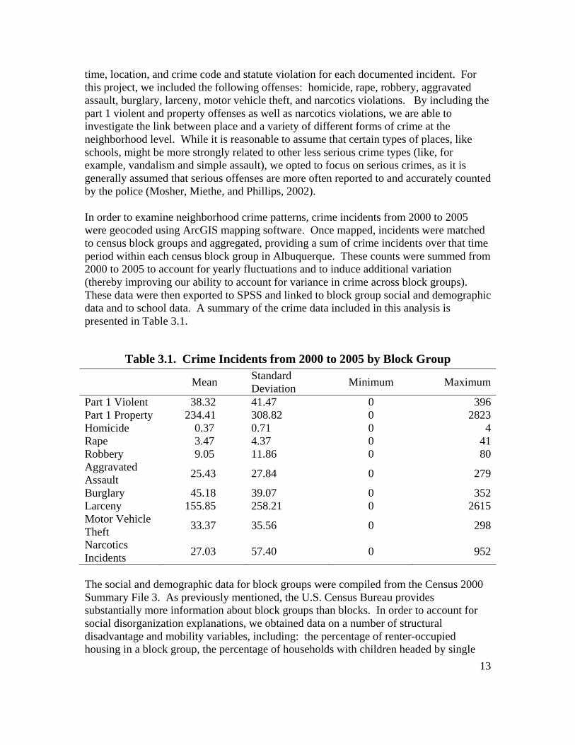
time, location, and crime code and statute violation for each documented incident. For this project, we included the following offenses: homicide, rape, robbery, aggravated assault, burglary, larceny, motor vehicle theft, and narcotics violations. By including the part 1 violent and property offenses as well as narcotics violations, we are able to investigate the link between place and a variety of different forms of crime at the neighborhood level. While it is reasonable to assume that certain types of places, like schools, might be more strongly related to other less serious crime types (like, for example, vandalism and simple assault), we opted to focus on serious crimes, as it is generally assumed that serious offenses are more often reported to and accurately counted by the police (Mosher, Miethe, and Phillips, 2002). In order to examine neighborhood crime patterns, crime incidents from 2000 to 2005 were geocoded using ArcGIS mapping software. Once mapped, incidents were matched to census block groups and aggregated, providing a sum of crime incidents over that time period within each census block group in Albuquerque. These counts were summed from 2000 to 2005 to account for yearly fluctuations and to induce additional variation (thereby improving our ability to account for variance in crime across block groups). These data were then exported to SPSS and linked to block group social and demographic data and to school data. A summary of the crime data included in this analysis is presented in Table 3.1.

Table 3.1. Crime Incidents from 2000 to 2005 by Block Group Mean Standard

Deviation Minimum Maximum

Part 1 Violent 38.32 41.47 0 396Part 1 Property 234.41 308.82 0 2823Homicide 0.37 0.71 0 4Rape 3.47 4.37 0 41Robbery 9.05 11.86 0 80Aggravated Assault 25.43 27.84 0 279

Burglary 45.18 39.07 0 352Larceny 155.85 258.21 0 2615Motor Vehicle Theft 33.37 35.56 0 298

Narcotics Incidents 27.03 57.40 0 952

The social and demographic data for block groups were compiled from the Census 2000 Summary File 3. As previously mentioned, the U.S. Census Bureau provides substantially more information about block groups than blocks. In order to account for social disorganization explanations, we obtained data on a number of structural disadvantage and mobility variables, including: the percentage of renter-occupied housing in a block group, the percentage of households with children headed by single

14

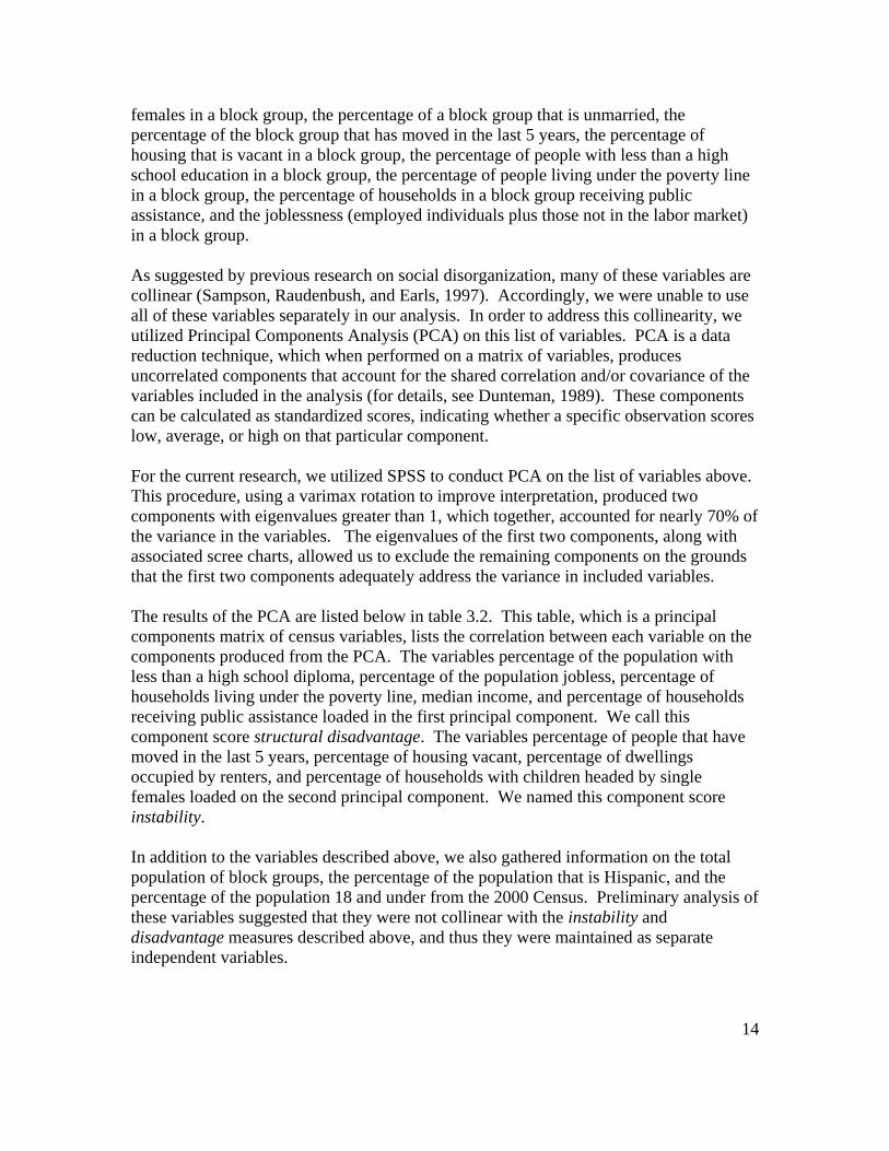
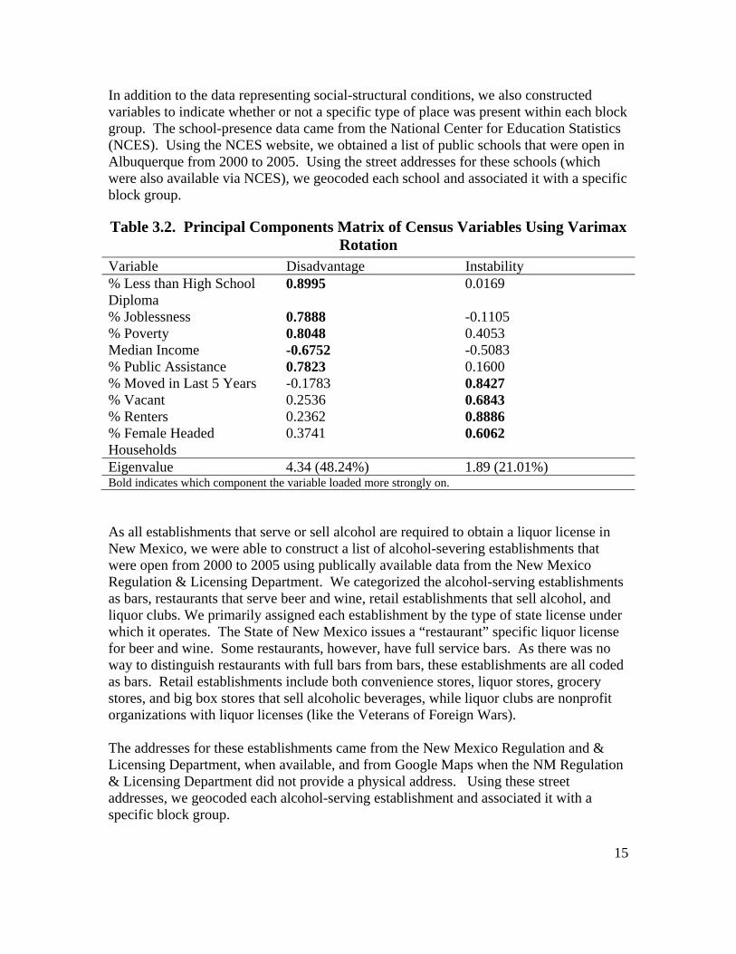
females in a block group, the percentage of a block group that is unmarried, the percentage of the block group that has moved in the last 5 years, the percentage of housing that is vacant in a block group, the percentage of people with less than a high school education in a block group, the percentage of people living under the poverty line in a block group, the percentage of households in a block group receiving public assistance, and the joblessness (employed individuals plus those not in the labor market) in a block group. As suggested by previous research on social disorganization, many of these variables are collinear (Sampson, Raudenbush, and Earls, 1997). Accordingly, we were unable to use all of these variables separately in our analysis. In order to address this collinearity, we utilized Principal Components Analysis (PCA) on this list of variables. PCA is a data reduction technique, which when performed on a matrix of variables, produces uncorrelated components that account for the shared correlation and/or covariance of the variables included in the analysis (for details, see Dunteman, 1989). These components can be calculated as standardized scores, indicating whether a specific observation scores low, average, or high on that particular component. For the current research, we utilized SPSS to conduct PCA on the list of variables above. This procedure, using a varimax rotation to improve interpretation, produced two components with eigenvalues greater than 1, which together, accounted for nearly 70% of the variance in the variables. The eigenvalues of the first two components, along with associated scree charts, allowed us to exclude the remaining components on the grounds that the first two components adequately address the variance in included variables. The results of the PCA are listed below in table 3.2. This table, which is a principal components matrix of census variables, lists the correlation between each variable on the components produced from the PCA. The variables percentage of the population with less than a high school diploma, percentage of the population jobless, percentage of households living under the poverty line, median income, and percentage of households receiving public assistance loaded in the first principal component. We call this component score structural disadvantage. The variables percentage of people that have moved in the last 5 years, percentage of housing vacant, percentage of dwellings occupied by renters, and percentage of households with children headed by single females loaded on the second principal component. We named this component score instability. In addition to the variables described above, we also gathered information on the total population of block groups, the percentage of the population that is Hispanic, and the percentage of the population 18 and under from the 2000 Census. Preliminary analysis of these variables suggested that they were not collinear with the instability and disadvantage measures described above, and thus they were maintained as separate independent variables.

15

In addition to the data representing social-structural conditions, we also constructed variables to indicate whether or not a specific type of place was present within each block group. The school-presence data came from the National Center for Education Statistics (NCES). Using the NCES website, we obtained a list of public schools that were open in Albuquerque from 2000 to 2005. Using the street addresses for these schools (which were also available via NCES), we geocoded each school and associated it with a specific block group.

Table 3.2. Principal Components Matrix of Census Variables Using Varimax Rotation

Variable Disadvantage Instability % Less than High School Diploma

0.8995 0.0169

% Joblessness 0.7888 -0.1105 % Poverty 0.8048 0.4053 Median Income -0.6752 -0.5083 % Public Assistance 0.7823 0.1600 % Moved in Last 5 Years -0.1783 0.8427 % Vacant 0.2536 0.6843 % Renters 0.2362 0.8886 % Female Headed Households

0.3741 0.6062

Eigenvalue 4.34 (48.24%) 1.89 (21.01%) Bold indicates which component the variable loaded more strongly on. As all establishments that serve or sell alcohol are required to obtain a liquor license in New Mexico, we were able to construct a list of alcohol-severing establishments that were open from 2000 to 2005 using publically available data from the New Mexico Regulation & Licensing Department. We categorized the alcohol-serving establishments as bars, restaurants that serve beer and wine, retail establishments that sell alcohol, and liquor clubs. We primarily assigned each establishment by the type of state license under which it operates. The State of New Mexico issues a “restaurant” specific liquor license for beer and wine. Some restaurants, however, have full service bars. As there was no way to distinguish restaurants with full bars from bars, these establishments are all coded as bars. Retail establishments include both convenience stores, liquor stores, grocery stores, and big box stores that sell alcoholic beverages, while liquor clubs are nonprofit organizations with liquor licenses (like the Veterans of Foreign Wars). The addresses for these establishments came from the New Mexico Regulation and & Licensing Department, when available, and from Google Maps when the NM Regulation & Licensing Department did not provide a physical address. Using these street addresses, we geocoded each alcohol-serving establishment and associated it with a specific block group.

16

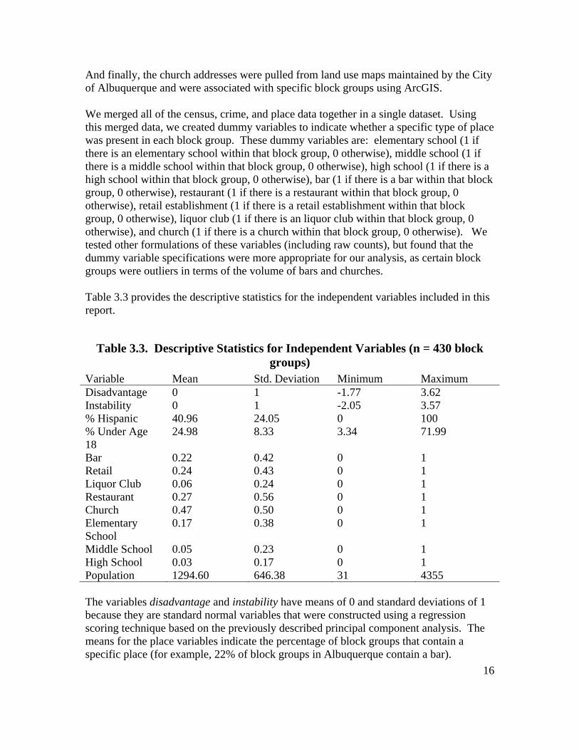
And finally, the church addresses were pulled from land use maps maintained by the City of Albuquerque and were associated with specific block groups using ArcGIS. We merged all of the census, crime, and place data together in a single dataset. Using this merged data, we created dummy variables to indicate whether a specific type of place was present in each block group. These dummy variables are: elementary school (1 if there is an elementary school within that block group, 0 otherwise), middle school (1 if there is a middle school within that block group, 0 otherwise), high school (1 if there is a high school within that block group, 0 otherwise), bar (1 if there is a bar within that block group, 0 otherwise), restaurant (1 if there is a restaurant within that block group, 0 otherwise), retail establishment (1 if there is a retail establishment within that block group, 0 otherwise), liquor club (1 if there is an liquor club within that block group, 0 otherwise), and church (1 if there is a church within that block group, 0 otherwise). We tested other formulations of these variables (including raw counts), but found that the dummy variable specifications were more appropriate for our analysis, as certain block groups were outliers in terms of the volume of bars and churches. Table 3.3 provides the descriptive statistics for the independent variables included in this report.

Table 3.3. Descriptive Statistics for Independent Variables (n = 430 block groups)

Variable Mean Std. Deviation Minimum Maximum Disadvantage 0 1 -1.77 3.62 Instability 0 1 -2.05 3.57 % Hispanic 40.96 24.05 0 100 % Under Age 18

24.98 8.33 3.34 71.99

Bar 0.22 0.42 0 1 Retail 0.24 0.43 0 1 Liquor Club 0.06 0.24 0 1 Restaurant 0.27 0.56 0 1 Church 0.47 0.50 0 1 Elementary School

0.17 0.38 0 1

Middle School 0.05 0.23 0 1 High School 0.03 0.17 0 1 Population 1294.60 646.38 31 4355 The variables disadvantage and instability have means of 0 and standard deviations of 1 because they are standard normal variables that were constructed using a regression scoring technique based on the previously described principal component analysis. The means for the place variables indicate the percentage of block groups that contain a specific place (for example, 22% of block groups in Albuquerque contain a bar).

17

Methods We utilize regression techniques to determine the relationship between place and crime at the block group level. Note, however, that because criminal incidents are discrete events and because many of the crime types covered in this analysis are heavily skewed to the right, traditional ordinary least squares regression techniques are inappropriate. Poisson regression, a variant of a generalized linear model, is typically preferred to ordinary least squares when dealing with count data (Osgood, 2000). Poisson regression models describe the relationship between a set of independent variables and the expected count of a dependent variable. The Poisson regression model, however, assumes that the mean is equal to the standard deviation. This is not the case for these data since all of the crime variables included in this analysis, with the exception of homicide, are over-dispersed (that is, they have a variance significantly greater than the mean). In these cases, it is common to utilize negative binomial regression (Osgood, 2000). Negative binomial regression possesses qualities similar to Poisson regression, while including an extra regression coefficient to account for overdispersion. Specifically, negative binomial regression maintains the same e to the b style of interpretation as Poisson regression. In the results chapter, the regression results dealing with homicide utilize Poisson regression, while the regression results dealing with all other dependent variables utilize negative binomial regression. All regression models were estimated using STATA software. Poisson and negative binomial regressions are utilized when the dependent variable is discrete. In this case, the dependent variables are crime counts. However, it is likely that block groups with more people have more crime. In order to account for this possibility, we control for population in our regression models. Instead of including population as a normal independent variable, which would suggest that population has a direct and substantively interesting relationship with crime counts, we include population as an exposure variable. The natural logarithm exposure variable is entered into the right hand side of Poisson or negative binomial regression and is given a fixed coefficient of one, which essentially changes Poisson and negative binomial regression from an analysis of crime counts to an analysis of crime rates per capita (Osgood, 2002: 27). We also addressed spatial dependency in each of the regression models presented in the results section of this paper. Spatial dependency is the idea that geographically close units are likely to be more similar to each other than to units that are geographically distant. Spatial dependency can come from multiple sources, including the artificial nature of census jurisdiction and “spillover.”1 Significant spatial dependency can lead to 1 Spatial dependency can result from census jurisdictions in that they may not accurately capture the active units of analysis. For example, suppose crime in a pair of block groups stems from a set of neighborhood processes and structures. If the block groups cut that neighborhood in half, then each of the block groups is expected to have a similar count of criminal incidents. Spatial dependency resulting from spillover suggest that geographic areas affect and are affected by neighboring areas. While conceptually distinct from the problem of artificial jurisdictions, spillover will also result in block groups that are

18

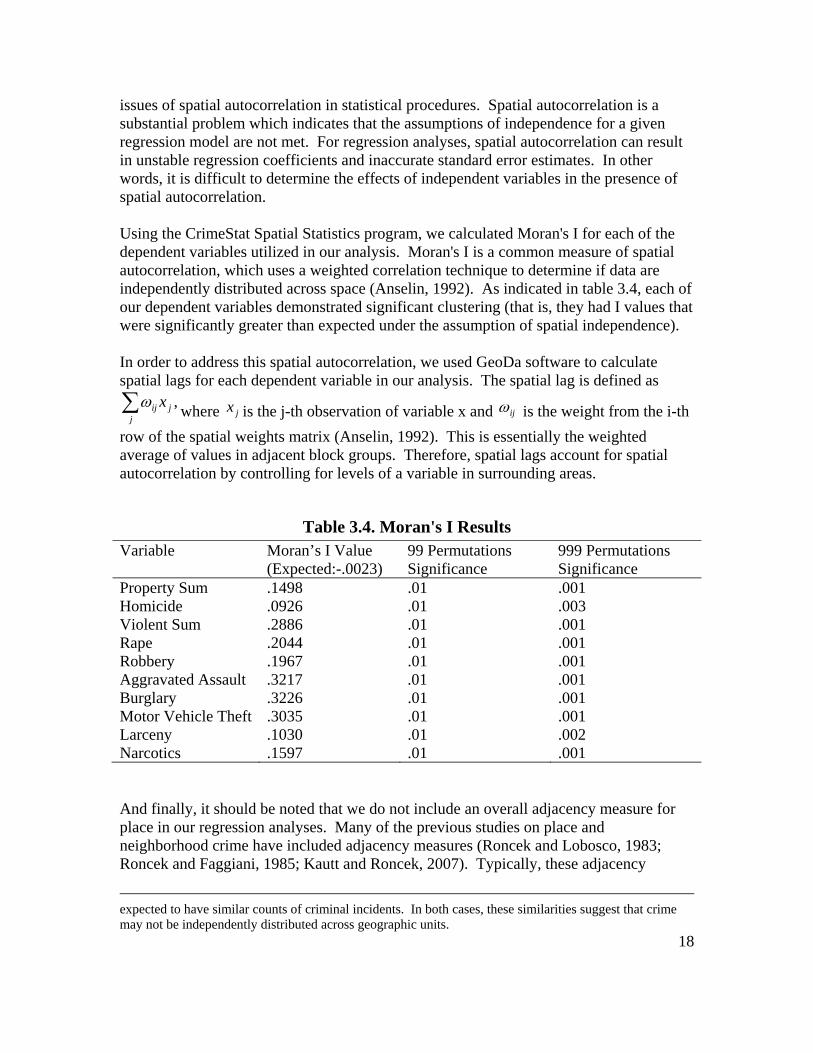
issues of spatial autocorrelation in statistical procedures. Spatial autocorrelation is a substantial problem which indicates that the assumptions of independence for a given regression model are not met. For regression analyses, spatial autocorrelation can result in unstable regression coefficients and inaccurate standard error estimates. In other words, it is difficult to determine the effects of independent variables in the presence of spatial autocorrelation. Using the CrimeStat Spatial Statistics program, we calculated Moran's I for each of the dependent variables utilized in our analysis. Moran's I is a common measure of spatial autocorrelation, which uses a weighted correlation technique to determine if data are independently distributed across space (Anselin, 1992). As indicated in table 3.4, each of our dependent variables demonstrated significant clustering (that is, they had I values that were significantly greater than expected under the assumption of spatial independence). In order to address this spatial autocorrelation, we used GeoDa software to calculate spatial lags for each dependent variable in our analysis. The spatial lag is defined as

,jj

ij x∑ω where jx is the j-th observation of variable x and ijω is the weight from the i-th row of the spatial weights matrix (Anselin, 1992). This is essentially the weighted average of values in adjacent block groups. Therefore, spatial lags account for spatial autocorrelation by controlling for levels of a variable in surrounding areas.

Table 3.4. Moran's I Results Variable Moran’s I Value

(Expected:-.0023) 99 Permutations Significance

999 Permutations Significance

Property Sum .1498 .01 .001 Homicide .0926 .01 .003 Violent Sum .2886 .01 .001 Rape .2044 .01 .001 Robbery .1967 .01 .001 Aggravated Assault .3217 .01 .001 Burglary .3226 .01 .001 Motor Vehicle Theft .3035 .01 .001 Larceny .1030 .01 .002 Narcotics .1597 .01 .001 And finally, it should be noted that we do not include an overall adjacency measure for place in our regression analyses. Many of the previous studies on place and neighborhood crime have included adjacency measures (Roncek and Lobosco, 1983; Roncek and Faggiani, 1985; Kautt and Roncek, 2007). Typically, these adjacency

expected to have similar counts of criminal incidents. In both cases, these similarities suggest that crime may not be independently distributed across geographic units.

19

measures are dummy variables that indicate whether or not an adjacent geographic unit (always the census block in previous research) contains a given place (e.g., is a block close to block that contains a school). This measure is typically intended to capture the effects of places on crime in nearby areas. We do not include any adjacency measures for two reasons. First, we are utilizing a larger unit of analysis. As block groups are made up of blocks, significant results in our analysis suggest that places influence crime in the block group, not just in the specific block in which they are located. Secondly, at this level of analysis, the vast majority of blocks are near block groups that contain a specific type of place. For example, 400 of the 432 block groups in Albuquerque are adjacent to one or more block groups that contain a school. Similarly, about 50% of block groups in Albuquerque contain a church and nearly 50% contain an alcohol-related establishment of some sort. In other words, at larger levels of aggregation, there is not enough variation to warrant the inclusion of an adjacency measure. Ultimately, this is a trade off for using the block group level of analysis. The block group allows us to control for more social and economic indicators and thus to give the social disorganization perspective a more thorough test. However, because block groups are larger and because the types of places included in our analysis are spread across Albuquerque, we are unable to test for adjacency effects and therefore can only make general conclusions about block groups and not about surrounding areas.

20

CHAPTER IV: RESULTS In order to investigate the relationship between place and crime at the block group level, we estimated a series of regression models using three dependent variables: violent crime, property crime, and narcotics incidents. The dependent variable Violent Crime is the number of the part 1 violent offenses that occurred in a given block group (that is, the sum of homicide, rape, aggravated assault, and robbery over 2000 to 2005). The dependent variable Property Crime is the number of the part 1 property offenses that occurred in a block group (that is, the sum of burglary, larceny, and motor vehicle theft). The dependent variable Narcotics is the number of drug possession and distribution arrests that occurred in a block group. The regression results for each dependent variable are presented in separate tables (Tables 4.1, 4.2, and 4.3) with five models. The five models include a control model (a regression model containing only control variables), a school model (a regression model containing control variables and dummy variables for the presence of elementary schools, middle schools, and high schools), a church model (a regression model containing control variables and the dummy variable for church presence), an alcohol model (a regression model including control variables and dummy variables for bars, retail establishments, liquor clubs, and restaurants), and a complete model (a regression model containing all of the above variables).2 All of the results presented below utilize negative binomial regression, as all of the models demonstrated significant overdispersion. We have included both pseudo R-squared values and negative log-likelihood (-2LL) values to indicate model fit. While the pseudo R-squared values are more readily interpretable, there are some technical problems with these statistics. 3 All comparisons of models are done using the log-likelihood ratio test. The test statistic for the log-likelihood ratio test is calculated as twice the negative difference of the log-likelihood values for two nested models and is assumed to have a chi-squared distribution with the degrees of freedom equal to the number of additional variables in the larger of the two nested models. If this test statistic is greater than a crucial chi-squared value with equal degrees of freedom, then the model with additional variables is said to improve the fit of the original model.

2 We also estimated a series of five regression models for each distinct crime type, in order to determine if there were important differences in the relationship between place and specific crime types. These supplementary regression models also use the negative binomial framework, except for the models utilizing homicide as the dependent variable. Homicide did not display substantial overdispersion, and thus we used Poisson regression to analyze homicide. In general these results are substantively similar to the results presented below. Tables displaying these regression results are included in Appendix A. 3 In some instances, pseudo R-squared measures have a maximum possible value that is less than 1, suggesting that these measures will be artificially lower than the traditional R-squared measure used in ordinary least squares regression (Dobson, 2002).

21

The regression coefficients in these tables are unstandardized negative binomial regression coefficients. As these coefficients are the expected change in the log of the expected count of y given a unit change in x, these coefficients are somewhat difficult to interpret in their unstandardized form. In order to facilitate interpretation, these coefficients are exponentiated prior to interpretation. This process changes the coefficients to the expected multiplicative change in the expected count of y. In other words, if the regression coefficient for variable X was 0.350 and this was exponentiated

)419.1( 350.0 =e , that would indicate that a 1-unit increase in X would correspond to a 41.9% increase in the expected count of Y.

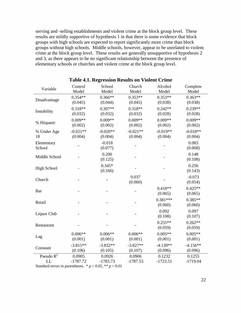
Place and Violent Crime Table 4.1 displays the regression results for violent crime. The coefficient for the spatial lag is statistically significant in all five models. This indicates that there is a significant amount of clustering of violent incidents. The control variables are all statistically significant as well. Block groups with higher levels of disadvantage and instability are expected to have significantly more violent crime than more advantaged and stable block groups. Block groups with larger Hispanic populations are also expected to report significantly more violent incidents, while block groups with larger youth populations are expected to report significantly fewer violent incidents. In terms of specific places, alcohol-related establishments have the largest statistically significant relationship with violent crime at the block group level. Block groups that contain bars, alcohol severing establishments, and restaurants that serve beer and wine are expected to report significantly more violent crime incidents than block groups without those types of places. The complete model indicates that block groups with bars are expected to report 53.0% ( 529.1425.0 =e ) more violent crime incidents than other block groups, controlling for other factors. Similarly, block groups with alcohol-selling establishments are expected to report 46.9% ( 469.1385.0 =e ) more violent crime incidents than block groups without alcohol-selling establishments, and block groups with restaurants that serve beer and wine are expected to report 30.0% ( 299.1262.0 =e ) more violent crime incidents than block groups without these types of restaurants. These results support hypotheses 4 and 5. Block groups with alcohol-serving and -selling establishments appear to have significantly more violent crime than block groups without these establishments. Furthermore, bars increase violent crime at the block group level more substantially than restaurants or liquor clubs. Schools and churches appear to be generally unrelated to violent crime at the block group level. The schools model suggests that block groups with high schools are expected to report significantly more violent crime incidents than block groups without high schools, but this relationship is not statistically significant in the complete model. This suggests that to the degree that there is a relationship between schools and violent crime at the block group level, this relationship is weaker than the relationship between alcohol-

22

serving and -selling establishments and violent crime at the block group level. These results are mildly supportive of hypothesis 1 in that there is some evidence that block groups with high schools are expected to report significantly more crime than block groups without high schools. Middle schools, however, appear to be unrelated to violent crime at the block group level. These results are generally unsupportive of hypothesis 2 and 3, as there appears to be no significant relationship between the presence of elementary schools or churches and violent crime at the block group level.

Table 4.1. Regression Results on Violent Crime

Variable Control Model

School Model

Church Model

Alcohol Model

Complete Model

Disadvantage 0.354** (0.045)

0.366** (0.044)

0.353** (0.045)

0.353** (0.038)

0.363** (0.038)

Instability 0.318** (0.032)

0.307** (0.032)

0.318** (0.032)

0.242** (0.028)

0.239** (0.028)

% Hispanic 0.009** (0.002)

0.009** (0.002)

0.009** (0.002)

0.009** (0.002)

0.009** (0.002)

% Under Age 18

-0.021** (0.004)

-0.020** (0.004)

-0.021** (0.004)

-0.019** (0.004)

-0.018** (0.004)

Elementary School - -0.018

(0.077) - - 0.083 (0.068)

Middle School - 0.200 (0.125) - - 0.148

(0.108)

High School - 0.345* (0.166) - - 0.256

(0.143)

Church - - 0.037 (0.060) - -0.073

(0.054)

Bar - - - 0.418** (0.065)

0.425** (0.065)

Retail - - - 0.381*** (0.060)

0.385** (0.060)

Liquor Club - - - 0.092 (0.108)

0.097 (0.107)

Restaurant - - - 0.255** (0.059)

0.262** (0.059)

Lag 0.006** (0.001)

0.006** (0.001)

0.006** (0.001)

0.005** (0.001)

0.005** (0.001)

Constant -3.815** (0.106)

-3.832** (0.105)

-3.827** (0.107)

-4.139** (0.096)

-4.156** (0.096)

Pseudo R2 0.0905 0.0926 0.0906 0.1232 0.1255 LL -1787.72 -1783.73 -1787.53 -1723.51 -1719.04

Standard errors in parentheses. * p < 0.05, ** p < 0.01

23

Log-likelihood ratio tests and the pseudo R-squared values confirm that alcohol-serving and -selling establishments are more important predictors of violent crime incidents than schools and churches. The pseudo R-squared value for the control model is 0.0905. This value increases to 0.0926 for the school model and 0.0906 for the church model. Conversely, the pseudo R-squared value for the alcohol model is 0.1232. Similarly, the log-likelihood test for the alcohol model ( 49.9,42.128 2

02 == χχ ) indicates that the

inclusion of places that serve and sell alcohol improves the fit of the control model at the 0.001 level of significance, while these tests suggest that schools ( 82.7,98.7 2

02 == χχ )

only improve the fit of the control model at the 0.05 level of significance, and churches ( 84.3,38.0 2

02 == χχ ) do not appear to significantly improve the fit of the control model

at any standard level of statistical significance. Similarly, the addition of schools and churches to the alcohol model does not statistically significantly improve the alcohol model’s fit ( 49.9,94.8 2

02 == χχ ).

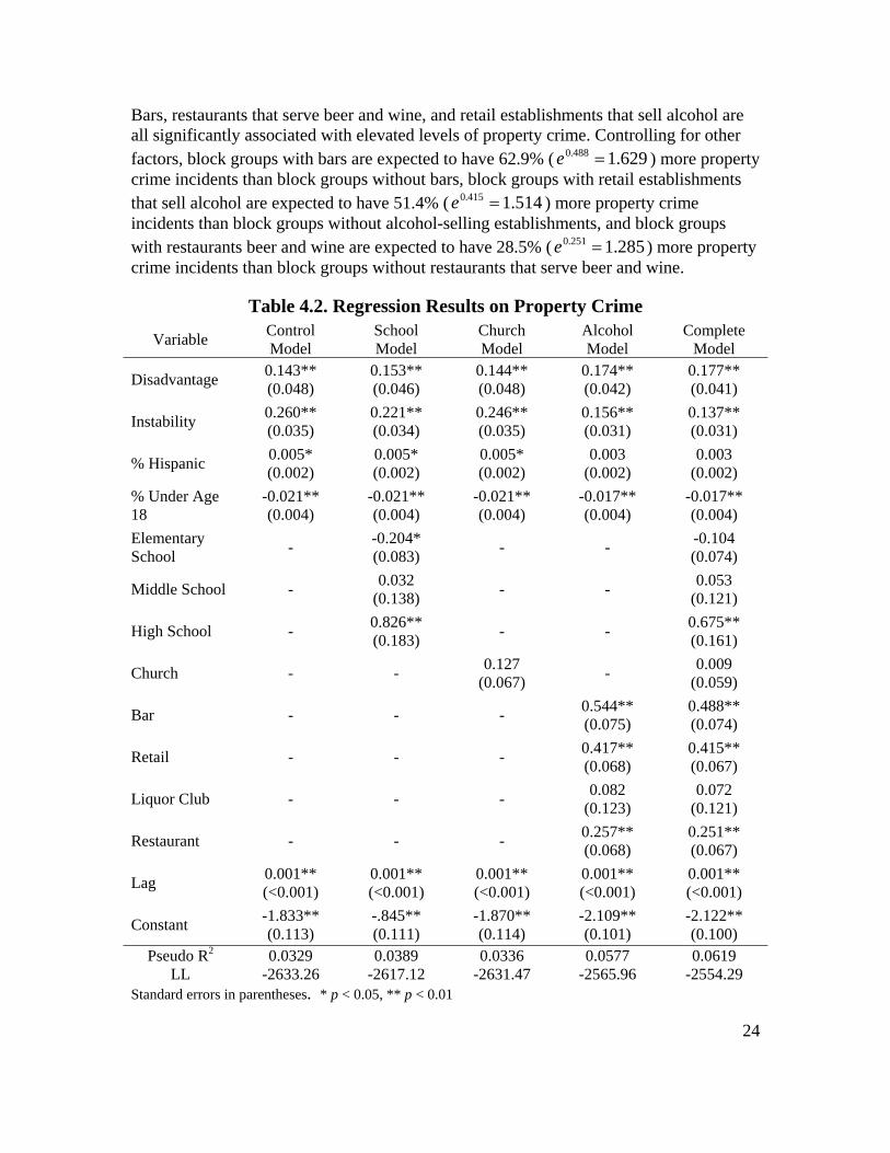
Place and Property Crime Table 4.2 displays the regression results for property crime. In terms of the control variables, many of these results are substantively similar to the results for violent crime. Block groups with higher levels of disadvantage and instability have higher property crime rates, while block groups with larger youth populations tend to have lower property crime rates. The spatial lag variable is statistically significant for this model as well, indicating that nearby block groups tend to have similar property crime rates, controlling for other factors. A key difference between the property and violent crime models is that the percentage of a block group’s population that is Hispanic is more strongly related to violent crime than to property crime. While there is evidence of a positive statistically significant relationship between percentage Hispanic and property crime, this relationship is not significant in all of the property crime models. In terms of place, there is a statistically significant relationship between schools and property crime and alcohol-serving and -selling establishments and property crime. Churches, however, are not significantly related to property crime. More specifically, block groups with high schools are expected to have 96.4% ( 964.1675.0 =e ) more property crime incidents than block groups without high schools, controlling for other factors. There is also evidence that block groups with elementary schools are expected to have significantly fewer property crimes than block groups without elementary schools, though elementary schools are not a significant predictor of property crime in the complete model. These results are generally supportive of our hypotheses regarding schools and crime, as they indicate that block groups with high schools have, controlling for other factors, more property crime, while block groups with elementary schools may, controlling for other factors, report less property crime.

24

Bars, restaurants that serve beer and wine, and retail establishments that sell alcohol are all significantly associated with elevated levels of property crime. Controlling for other factors, block groups with bars are expected to have 62.9% ( 629.1488.0 =e ) more property crime incidents than block groups without bars, block groups with retail establishments that sell alcohol are expected to have 51.4% ( 514.1415.0 =e ) more property crime incidents than block groups without alcohol-selling establishments, and block groups with restaurants beer and wine are expected to have 28.5% ( 285.1251.0 =e ) more property crime incidents than block groups without restaurants that serve beer and wine.

Table 4.2. Regression Results on Property Crime

Variable Control Model

School Model

Church Model

Alcohol Model

Complete Model

Disadvantage 0.143** (0.048)

0.153** (0.046)

0.144** (0.048)

0.174** (0.042)

0.177** (0.041)

Instability 0.260** (0.035)

0.221** (0.034)

0.246** (0.035)

0.156** (0.031)

0.137** (0.031)

% Hispanic 0.005* (0.002)

0.005* (0.002)

0.005* (0.002)

0.003 (0.002)

0.003 (0.002)

% Under Age 18

-0.021** (0.004)

-0.021** (0.004)

-0.021** (0.004)

-0.017** (0.004)

-0.017** (0.004)

Elementary School - -0.204*

(0.083) - - -0.104 (0.074)

Middle School - 0.032 (0.138) - - 0.053

(0.121)

High School - 0.826** (0.183) - - 0.675**

(0.161)

Church - - 0.127 (0.067) - 0.009

(0.059)

Bar - - - 0.544** (0.075)

0.488** (0.074)

Retail - - - 0.417** (0.068)

0.415** (0.067)

Liquor Club - - - 0.082 (0.123)

0.072 (0.121)

Restaurant - - - 0.257** (0.068)

0.251** (0.067)

Lag 0.001** (<0.001)

0.001** (<0.001)

0.001** (<0.001)

0.001** (<0.001)

0.001** (<0.001)

Constant -1.833** (0.113)

-.845** (0.111)

-1.870** (0.114)

-2.109** (0.101)

-2.122** (0.100)

Pseudo R2 0.0329 0.0389 0.0336 0.0577 0.0619 LL -2633.26 -2617.12 -2631.47 -2565.96 -2554.29

Standard errors in parentheses. * p < 0.05, ** p < 0.01

25

These results are supportive of our hypotheses regarding alcohol serving and selling establishments and crime in that block groups with alcohol-selling and -serving establishments are expected to report significantly higher counts of property crime, though this effect is larger for bars than for other types of alcohol-related establishments. Interestingly, however, the effect of high school presence on property crime is larger than the effect of bars on property crime. Log-likelihood ratio tests and the pseudo R-squared values indicate that alcohol serving and selling establishments are more important predictors of property crime incidents than schools, which in turn are more important than churches. The difference in both pseudo R-squared values and in log-likelihoods is larger for the alcohol model than it is for the schools model. This result seems contrary to the result that the regression coefficient for high schools is larger than the regression coefficient for any other type of place. This apparent difference may reflect the fact that several different types of alcohol severing and selling establishments are significantly related to crime in the complete model, while high schools are the only type of school that is consistently related to property crime.

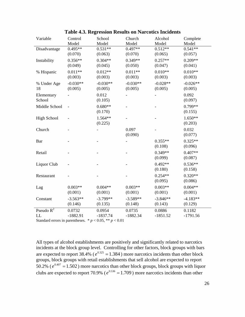
Place and Narcotics Crime Table 4.3 displays the regression results for narcotics incidents. In terms of control variables, these results are substantively very similar to the results for violent and property crime. The spatial lag variable is again statistically significant across all models, indicating that nearby block groups tend to be similar in terms of narcotics incidence rates. Block groups with higher levels of disadvantage, instability, and greater proportions of Hispanic residents report significantly more narcotics incidents than other block groups. Conversely, block groups with larger proportions of youths report significantly fewer narcotics incidents than other block groups. In terms of place, there is again no statistically significant relationship between the presence of a church and narcotics incidents at the block group level. Both schools and alcohol-serving and -selling establishments are significantly related to narcotics incidents at the block group level. Regarding schools, block groups with high schools are expected to report 420.7% ( 207.5650.1 =e ) more narcotics incidents than block groups without high schools, while block groups with middle schools are expected to report 122.3% ( 223.2799.0 =e ) more narcotics incidents than block groups without middle schools. Elementary schools are not significantly related to narcotics incidents. Block groups with high schools and middle schools have elevated rates of narcotics incidents, though the presence of a high school is a much larger risk factor than the presence of a middle school. These results are generally supportive of our hypotheses regarding the relationship between schools and neighborhood crime, though we do not observe any protective effect of elementary schools on narcotics at the block group level.

26

Table 4.3. Regression Results on Narcotics Incidents Variable Control

Model School Model

Church Model

Alcohol Model

Complete Model

Disadvantage 0.495** (0.070)

0.531** (0.063)

0.497** (0.070)

0.512** (0.065)

0.541** (0.057)

Instability 0.356** (0.049)

0.304** (0.045)

0.349** (0.050)

0.257** (0.047)

0.209** (0.041)

% Hispanic 0.011** (0.003)

0.012** (0.003)

0.011** (0.003)

0.010** (0.003)

0.010** (0.003)

% Under Age 18

-0.030** (0.005)

-0.030** (0.005)

-0.030** (0.005)

-0.028** (0.005)

-0.026** (0.005)

Elementary School

- 0.012 (0.105)

- - 0.092 (0.097)

Middle School - 0.680** (0.170)

- - 0.799** (0.155)

High School - 1.564** (0.225)

- - 1.650** (0.203)

Church - - 0.097 (0.090)

- 0.032 (0.077)

Bar - - - 0.355** (0.108)

0.325** (0.096)

Retail - - - 0.349** (0.099)

0.407** (0.087)

Liquor Club - - - 0.492** (0.180)

0.536** (0.158)

Restaurant - - - 0.254** (0.095)

0.320** (0.086)

Lag 0.003** (0.001)

0.004** (0.001)

0.003** (0.001)

0.003** (0.001)

0.004** (0.001)

Constant -3.563** (0.146)

-3.799** (0.135)

-3.589** (0.148)

-3.846** (0.143)

-4.183** (0.129)

Pseudo R2 0.0732 0.0954 0.0735 0.0886 0.1182 LL -1882.91 -1837.74 -1882.34 -1851.52 -1791.56 Standard errors in parentheses. * p < 0.05, ** p < 0.01 All types of alcohol establishments are positively and significantly related to narcotics incidents at the block group level. Controlling for other factors, block groups with bars are expected to report 38.4% ( 384.1325.0 =e ) more narcotics incidents than other block groups, block groups with retail establishments that sell alcohol are expected to report 50.2% ( 502.1407.0 =e ) more narcotics than other block groups, block groups with liquor clubs are expected to report 70.9% ( 709.1536.0 =e ) more narcotics incidents than other

27

block groups, and block groups with restaurants that serve beer and wine are expected to report 37.7% ( 377.1320.0 =e ) more narcotics incidents than other block groups. These results are highly supportive of our general hypothesis regarding alcohol establishments and crime, as block groups containing alcohol establishments are expected to report significantly more narcotics incidents than block groups without alcohol establishments. Our results, however, are not supportive of hypothesis 5 regarding the importance of bars. In terms of narcotics incidents, both retail establishments that sell alcohol and liquor clubs are a larger risk factor for narcotics incidents at the block group level than bars. Interestingly, log-likelihood ratio tests and the pseudo R-squared values indicate that schools are a more important predictor of narcotics incidents than alcohol establishments. The difference in the pseudo R-squared values and in log-likelihoods is larger between the alcohol model and control model than it is between the school and control model. Moreover, the regression coefficient for high schools is the largest of all place variables and the regression coefficient for middle schools is the second largest. While schools may have a larger effect on narcotics incidents at the block group level, alcohol establishments are still important. Each of the alcohol variables is a significant predictor of narcotics incidents at the block group level and the log-likelihood test comparing the school and complete models suggests that the inclusion of the alcohol establishment variables significantly improves the school model’s fit ( 07.11,36.92 2

02 == χχ ).

28

CHAPTER V: DISCUSSION AND CONCLUSION The results of our regression analyses indicate that alcohol establishments and certain types of schools are risk factors for crime at the block group level. Specifically, our results indicate that block groups that contain alcohol establishments and, to a lesser degree, block groups that contain high schools report more crime. It is important to note that these results hold independent of the structural conditions of block groups. By utilizing the block group level of analysis, we were able to include measures to statistically control for structural disadvantage, residential instability, and demographic factors. That there is still a strong, statistically significant relationship between different types of places and crime, even after controlling for these factors, indicates that the relationship between place and crime is not spurious by way of block group characteristics. In terms of schools, our regression results indicate that block groups with high schools are likely to report more property and narcotics crime, controlling for other factors. In fact, the regression coefficients for high schools are larger than the regression coefficients for any other types of place, suggesting that high school presence is the strongest place predictor of property and narcotics crime. Middle schools, though generally unrelated to violent and property crime in our models, are the second strongest predictor of narcotics incidents. These results support our first hypothesis, though it should be reiterated that high schools are a much more salient predictor of neighborhood crime than middle schools. These results make sense in the context of the routine activities perspective. Individuals in the high school age group are, as previously mentioned, at an increased risk to be both the victims and offenders of property crime (Hirschi and Gottfredson, 1983; Farrington, 1986; Rand and Catalano, 2007). Given that people from these age groups converge in large numbers in and around schools, it is unsurprising that areas with high schools have elevated property crime rates. Nationwide, the Centers for Disease Control and Prevention estimates that approximately 20% of teenagers admit to at least occasionally using some illegal drug (Eaton et al., 2010), so it seems sensible that drug dealers would attempt to converge with their potential clients in and around schools. From a social disorganization perspective, our results may indicate that high schools, and to a lesser degree, middle schools impede neighborhood collective efficacy processes. Unfortunately, we do not have access to the type of data necessary to explore this possibility. Future research should investigate the degree to which block groups with high schools differ from other block groups in terms of key measures of social organization (e.g., participation in local community groups and social network measures). In terms of alcohol establishments, bars, restaurants that serve beer and wine, and retail establishments that sell alcohol are significant predictors of violent, property, and

29

narcotics crime at the block group level. Liquor clubs, conversely, are only significantly related to narcotics offenses. Narcotics incidents are not associated with specific victims. This might suggest that while liquor clubs do promote the convergence of people in time and space, these clubs are not promoting the convergence of people that are likely to victimize each other. The other types of alcohol establishments are associated with elevated levels of violent, property, and drug crime. This finding clearly fits within the framework of the routine activities perspective, as each of these types of places brings together large groups of people. Bars are the largest place predictor of violent crime at the block group level and the second largest place predictor of property crime at the block group level. These findings generally support our fifth hypothesis and indicate that bars have a greater criminogenic effect than other alcohol establishments. Unfortunately, we are unable to specify exactly why bars are such a significant risk factor for crime at the block group level. It may be the case, as Roncek and Maier (1991) have previously argued, that the consumption of alcohol at bars increases both the average criminal motivation and target attractiveness of bar patrons. Alternatively, the relationship between bars and neighborhood crime may be reflective of some selection effect in that people who are likely to engage in and be the victims of crime are simply more likely to frequent bars than other people. Bars may also interfere with collective efficacy processes by impeding the formation or reducing the strength of neighborhood-level informal social controls. Local patrons may be less beholden to neighborhood-level social controls when under the influence of alcohol. Additionally, local social controls likely hold little sway over patrons from outside the neighborhood. Interestingly, retail establishments that sell alcohol are also significantly related to crime at the block group level. While the retail establishments include places that would be traditionally defined as liquor stores, the majority of places that possess this type of liquor license in Albuquerque are better viewed as big box and grocery stores. Clearly, the above arguments regarding bars and neighborhood crime do not cleanly apply to big box stores or grocery stores. It is possible that the relationship between retail establishments that sell alcohol and neighborhood crime is simply reflective of the sheer volume of people that converge in and around these locations, many of whom may come from outside the neighborhood. Future research should compare the criminogenic properties of retail establishments that serve alcohol to those that do not. Our results indicate that there is no statistically significant relationship between the presence of religious places and crime at the block group level. This result contradicts our hypothesis regarding religious places and crime at the block group level. Based on the routine activities and social disorganization traditions, we had expected religious places to have a negative relationship with block group crime, as we believed that churches might promote routine activity patterns that are not conducive to crime, while simultaneously promoting the formation of pro-social friendship networks. While we were unable to find any evidence of a protective role for churches, we believe that the potential relationship between churches and neighborhood crime deserves additional

30

study. The measure of religious places that we employed in our analysis (the presence or absence of a place of worship in a block group) may be too simplistic to evaluate the role of churches in terms of neighborhood crime. The presence of a religious place does not indicate the usage of that place within a neighborhood. Certain religious places may be busier than other churches and this level of usage may be reflective of how effective a religious place can be in terms of the promotion of social ties. Some religious places may, for example, be more heavily involved in their neighborhoods than others. Further, some religious places, especially those that serve homeless and felon populations, may in fact increase crime at the neighborhood level by promoting the convergence of these populations in time and space. Perhaps more importantly, our measure of religious places cannot distinguish between different types of religious places. Our measure simply indicates whether or not there is at least one religious place within a block group, but it does not indicate the religious affiliation of these religious places within a block group. While it is true that most of the churches in Albuquerque are Christian in nature, our measure is also unable to distinguish between different types of Christian churches. DiIolio (2009: 129), for example, notes that most theory and research on religion and crime approaches the issue from a “churched/not churched” perspective. He notes, however, that there are several types of religious organizations and suggests that these organizations may be differentially related to crime. It is important for future research on religious places and neighborhood crime to distinguish between different types of religious places and, if possible, to incorporate data on the use of these places (both in terms of frequency and types of services offered). In general, our results suggest that specific types of places are risk factors for neighborhood crime. Elementary schools are the only type of place included in our study that has a statistically significant negative relationship with property crime at the block group level. This result, however, is not as strong as the positive relationships described above (elementary schools are significant in the school model, but not in the complete model). Given that we controlled for a wide variety of other factors, this result may suggest that the presence of elementary schools may reduce property crime. Both the social disorganization and routine activities perspectives provide arguments that might explain the protective role of elementary schools. Unlike middle schools and high schools, elementary schools do not funnel large groups of people in neighborhoods that, on average, are more likely to be criminal offenders and victims. In other words, elementary school students are not likely to engage in property crime, nor are they likely to be the victims of property offenses. Further, the smaller student-to-teacher ratio and higher degree of parental involvement in elementary schools may foster both a heightened level of guardianship and the formation of positive social ties, both of which may serve to hinder property crime. Interestingly, the presence of elementary schools is not associated with lower levels of violent crime or drug crime. Controlling for other factors, there is no statistically significant relationship between elementary school presence and these types of crimes,

31

suggesting that block groups with elementary schools are no different than other block groups in terms of violent crime or drug crime. We are unable to state why elementary schools seem to protect block groups against property crime and not violent or drug crime. The routine activities perspective would suggest that elementary schools promote routine activity patterns that are discouraging to the commission of property crime and that are neither conducive nor discouraging to violent crime and drug crime. Similarly, the social disorganization perspective might argue that elementary schools produce informal social control that is effective at deterring property crime but not violent or drug crime. It may be the case, for example, that elementary schools promote a specific style of guardianship and a specific style of social control, both focused on the monitoring of elementary school students. That is, perhaps the protective role of elementary schools is directly related to the presence and visual supervision of teachers and parents. The presence of these individuals may deter would-be burglars, as it may be difficult to break into homes in these neighborhoods. On the other hand, drug crimes and the serious sort of violent crimes that we considered in our analysis may be more likely to occur behind closed doors and are thus less likely to be deterred by the presence of teachers and parents. Moreover, if elementary schools primarily promote social organization for the monitoring and protection of elementary school-aged children, it may be the case that elementary schools do not foster the types of social bonds that are likely to deter other types of crime. Future research on place and neighborhood crime should attempt to address this issue and more completely describe the processes through which specific places influence neighborhood crime. For example, it would be useful to better understand how neighborhoods with and without elementary schools vary in terms of routine activity patterns and overall social organization. If, as we speculated above, elementary schools promote a type of social control based on the supervision of public spaces, we might expect neighborhoods with elementary schools to have more active neighborhood watches and neighborhood association groups and yet not necessarily denser pro-social friendship networks. While we have advocated for a more thorough examination of how elementary schools shape neighborhood activity patterns and neighborhood organization, we believe that this approach can improve the criminological knowledge on place and crime more broadly. To date, most research on place and crime, including the current study, has simply demonstrated that there is an empirical correlation between the presence of certain types of places and neighborhood crime rates. This research, while useful, is only a first step toward understanding the relationship between place and crime. Beyond describing which types of places are, on average, positively or negative related to crime, future research, utilizing neighborhood surveys and qualitative data, should focus on describing how these places are related to crime. This knowledge may both highlight the conditional scopes of theoretical traditions and be useful in the development of place-specific crime prevention strategies.

32

These results highlight several policy implications on neighborhood crime. First, given the robust and highly significant relationship between the presence of bars and all types of crime, we believe that public policy makers should focus special attention on neighborhoods containing bars. The routine activities perspective suggests that these areas are likely to see elevated crime rates due to the fact that there is not enough capable guardianship in and around bars to counter the convergence of the large volume of would-be victims and offenders. The obvious policy implications are to either increase levels of guardianship (increased security in and around bars and increased police presence in these neighborhoods) or to decrease the number of motivated offenders and suitable victims (this may be possible, for example, by imposing capacity limitations in bars based on crime instead of fire considerations). Other target hardening strategies, like increased street lighting and the placement of security cameras may also be useful in reducing crime in and around bars. Furthermore, neighborhood associations and related watch groups may be able to provide important support for these efforts, by extending their watch and influence to both public and commercial areas. Many of these strategies may also be useful in addressing the moderately strong relationship between the presence of restaurants that serve alcohol and crime. Similarly, these results suggest that additional attention to neighborhoods with high schools, and to a lesser extent, to neighborhoods with middle schools is warranted. Many of the policy implications for neighborhoods with bars also apply to neighborhoods with schools. These neighborhoods may benefit from an increased presence of teachers, school security, and police officers in and around schools, especially during the commutes to and from schools. Neighborhood associations and watch groups near high schools may also be able to reduce the criminogenic effect of these schools by carefully scheduling watch activities before and after school in the areas surrounding the schools. These strategies would expand the scope of guardianship to include both the school grounds and the surrounding areas. We believe that it is important for future research to study specific situational crime strategies and neighborhood organizational patterns to better develop a list of which strategies and approaches are most effective at reducing the criminogenic effects of specific types of places. We conclude by noting that our research has several limitations that must be mentioned. While we believe that our results are explainable from the routine activities and social disorganization perspectives, we do not have actual measures of these processes. Further, we have focused largely on serious offenses as we do not have access to geocoded data for less serious types of crimes. It may be the case that our results would not apply to less serious violent and property offenses. Future research should investigate the relationship between place and less serious forms of crime. Despite these limitations, we feel that the current research is valuable in many ways. This research has demonstrated that alcohol establishments and schools are associated with certain types of crime at the block group level, even after controlling for a number of factors that are known to be associated with crime. Most of the previous research on

33

place and crime has been either completely descriptive (calculating the proportion of incidents that happen at specific places) or has been conducted at the block level of analysis (which precludes controlling for a wide range of social structural variables).

34

REFERENCES Alvarez-Rivera, Lorna L., Fox, Kathleen A. (2010). Institutional attachments and self-control: Understanding deviance among Hispanic adolescents. Journal of Criminal Justice 38,666-674. Anselin, L. (1992). Spatial data analysis with GIS: An introduction to application in the social sciences. Santa Barbara, CA: National Center for Geographic Information and Analysis, University of California. Block, R. and Block C.R. (1995). Space, place, and crime: Hot spots areas and hot places of liquor-related crime. In J. Eck and D. Weisburd, (Eds.), Crime and place (pp. 145–183). Monsey, NY: Criminal Justice Press. Broidy, L., Willits, D., and Denman, K. (2009). Schools and neighborhood crime (Final Report to the Justice Research Statistics Association). Albuquerque: New Mexico Statistical Analysis Center, Institute for Social Research, University of New Mexico.

Bursik, R. (1988). Social disorganization and theories of crime and delinquency: Problems and prospects. Criminology, 26, 519–552. Cohen, L. E. and Felson, M. (1979). Social change and crime rate trends: A routine activity approach. American Sociological Review, 44, 588–608. DiIolio, J. (2009). More religion, less crime? Science, felonies, and the three faith factors. Annual Review of Law and Social Science, 5, 115–133. Dobson, A. J. (2002). An introduction to generalized linear models. Florida: Chapman & Hall/CRC Press. Dunteman, G. (1989). Principal components analysis. Newbury Park, California: Sage. Eaton, D., Kann, L., Kinchen, S., Shanklin, S., Ross, J., Hawkins, J., Harris, W., Lowry, R, McManus, T., Chyen, D., Lim, C., Whittle, L., Brener, N., and Wechsler H. (2010). Youth risk behavior surveillance – United States, 2009. Surveillance Summaries, 59, 1-142. Eccles, J. S. and Harold, R. D. (1996). Family involvement in children’s and adolscents’ schooling. In J. D. A Booth (Ed.), Family-school links: How do they affect educational outcomes (pp 3–34). Hillsdale, NJ: Lawrence Erlbaum Associates. Farrington, D. (1986). Age and crime. Crime and Justice, 7, 189–250.

35

Garofalo, J., Siegel, L., and Laub, J. (1987). School-related victimizations among adolescents: An analysis of National Crime Survey (NCS) narratives. Journal of Quantitative Criminology, 3, 321–338. Hill, N. E. and Taylor, L. C. (2004). Parental school involvement and children’s academic achievement: Pragmatics and issues. Current Directions in Psychological Science, 13, 161–164. Hirschi, T., and Gottfredson, M. (1983). Age and the explanation of crime. American Journal of Sociology 89, 552-584. Ito, T. A., Miller, N., and Pollock, V. E. (1996). Alcohol and aggression: A meta-analysis on the moderating effects of inhibitory cues, triggering events, and self-focused attention. Psychological Bulletin, 120, 60–82. Johnson, Byron R., Jang, Sung Joon, De Li, Spencer, Larson, David. (2000). The ‘Invisible Institution’ and Black Youth Crime: The Church as an Agency of Local Social Control. Journal of Youth and Adolescence 29, 479-498 Kasarda, J. and Janowitz, M. (1974). Community attachment in mass society. American Sociological Review, 39, 28–39 Kautt, P. M. and Roncek, D. W. (2007). Schools as criminal “hot spots”: Primary, secondary, and beyond. Criminal Justice Review, 32, 339–357. Knudten, Richard D., Knudten, Mary S. (1971). Juvenile Delinquency, Crime, and Religion. Review of Religious Research 12,130-152 Krivo, L., and Peterson, R. (1996). Extremely disadvantaged neighborhoods and urban crime. Social Forces, 75, 619-650. Lee, M. (2006). The religious institutional base and violent crime in rural areas. Journal for the Scientific Study of Religion, 45, 309–324. Lee, M. 2008. Civic community in the hinterland: Toward a theory of rural social structure and violence. Criminology, 46, 447–478. Lee, M. (2010). Civic community, population change, and violent crime in rural communities. Journal of Research in Crime and Delinquency, 47, 118–147. Mosher, C. J., Miethe, T. D., and Phillips, D. M. (2002). The mismeasure of crime. Thousand Oaks, CA: Sage Publications.

36

Murray, R. and Swatt, M. (2010). Disaggregating the relationship between schools and crime: A spatial analysis. Crime & Deliqnuency. Available online < http://cad.sagepub.com/content/early/2010/01/05/0011128709348438>. Osgood, D. W. (2000). Poisson-based regression analysis of aggregate crime rates. Journal of Quantitative Criminology, 16, 21–43. Peterson, R., Krivo, L., and Harris, M.. (2000). Disadvantage and neighborhood violent crime: Do local institutions matter? Journal of Research in Crime and Delinquency, 37, 31–63. Rand, M. and Catalano, S. (2007). Criminal victimization, 2006. Washington, DC: U.S. Department of Justice. Roman, C.G. (2004). Schools, neighborhoods, and violence: Crime within the daily routines of youth. Lanham, MD: Lexington Books. Roncek, D.W. (1981). Dangerous places: Crime and residential environment. Social Forces, 60, 74–96. Roncek, D.W. and Bell, R. (1981). Bars, blocks, and crime. Journal of Environmental Systems, 11, 35–47. Roncek, D.W. and Faggiani, D. (1985). High schools and crime: A replication. Sociological Quarterly, 26, 491–505. Roncek, D.W. and Lobosco, A. (1983). Effect of high schools on crime in their neighborhoods. Social Science Quarterly, 64(3), 598–613. Roncek, D.W. and Maier, P.A. (1991). Bars, blocks, and crimes revisited: Linking the theory of routine activities to the empiricism of “hot spots.” Criminology, 29, 725–753. Roncek, D. W. and Pravatiner, M. A. (1989). Additional evidence that taverns enhance nearby crime. Sociology and Social Research, 73, 185–188. Rose, Dina R., Clear, Todd R. (2006). Incarceration, Social Capital, and Crime: Implications for Social Disorganization Theory. Criminology 36, 441-480 Sampson, R. J. and Groves, W. B. (1989). Community structure and crime: Testing social-disorganization theory. American Journal of Sociology, 94, 774–802. Sampson, R. J. and Wilson,W. J. (1995). Toward a theory of race, crime, and urban inequality. In J. Hagon and R. D. Peterson (Eds.), Crime and inequality (pp. 37–54). Stanford, CA: Stanford University Press.

37

Sampson, R. J., Morenoff, J. D., and Gannon-Rowley, T. (2002). Assessing “neighborhood effects”: Social processes and new directions in research. Annual Review of Sociology, 28, 443–478. Sampson, R. J., Raudenbush, S. W., and Earls, F. (1997). Neighborhoods and violent crime: A multilevel study of collective efficacy. Science, 277, 918–924. Shaw, C. and McKay, H. (1942). Juvenile delinquency and urban areas. Chicago: University of Chicago Press. Sherman, L. W., Gartin, P. R., and Buerger, M. E. (1989). Hot spots of predatory crime: Routine activities and the criminology of place. Criminology, 27(1): 27– 56. Spelman, W. (1995). Criminal careers of public places. In J. Eck and D. Weisburd (Eds.), Crime and place (pp. 115–144). Monsey, NY: Criminal Justice Press. Taylor, Robert Joseph, Thornton, Michael C., Chatters, Linda M. (1988). Black Americans’ Perceptions of the Sociohistorical Role of the Church. Journal of Black Studies 18, 123-138 Taylor, Robert Joseph, Chatters, Linda M. (1988). Church Members as a Source of Informal Social Support. Review of Religious Research 30, 193-203. Wimberly, E. (1979). Pastoral Care in the Black Church. Nashville: Adingdon.

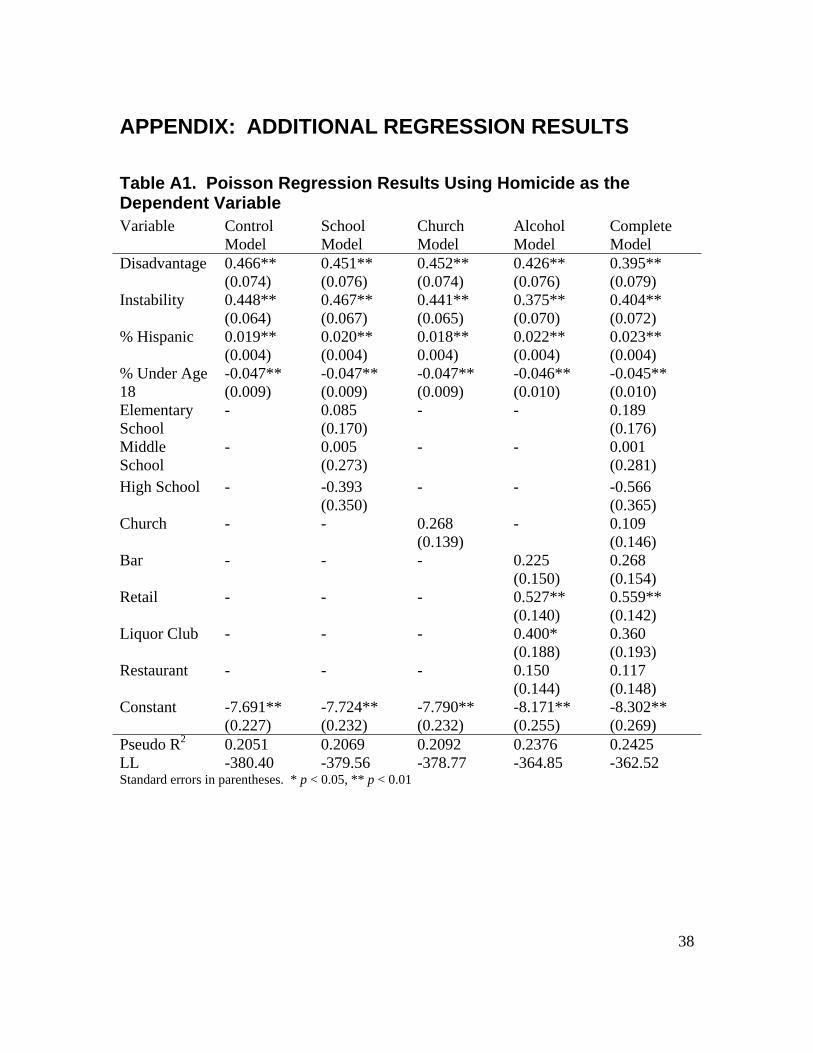
38

APPENDIX: ADDITIONAL REGRESSION RESULTS

Table A1. Poisson Regression Results Using Homicide as the Dependent Variable Variable Control

Model School Model

Church Model

Alcohol Model

Complete Model

Disadvantage 0.466** (0.074)

0.451** (0.076)

0.452** (0.074)

0.426** (0.076)

0.395** (0.079)

Instability 0.448** (0.064)

0.467** (0.067)

0.441** (0.065)

0.375** (0.070)

0.404** (0.072)

% Hispanic 0.019** (0.004)

0.020** (0.004)

0.018** 0.004)

0.022** (0.004)

0.023** (0.004)

% Under Age 18

-0.047** (0.009)

-0.047** (0.009)

-0.047** (0.009)

-0.046** (0.010)

-0.045** (0.010)

Elementary School

- 0.085 (0.170)

- - 0.189 (0.176)

Middle School

- 0.005 (0.273)

- - 0.001 (0.281)

High School - -0.393 (0.350)

- - -0.566 (0.365)

Church - - 0.268 (0.139)

- 0.109 (0.146)

Bar - - - 0.225 (0.150)

0.268 (0.154)

Retail - - - 0.527** (0.140)

0.559** (0.142)

Liquor Club - - - 0.400* (0.188)

0.360 (0.193)

Restaurant - - - 0.150 (0.144)

0.117 (0.148)

Constant -7.691** (0.227)

-7.724** (0.232)

-7.790** (0.232)

-8.171** (0.255)

-8.302** (0.269)

Pseudo R2 0.2051 0.2069 0.2092 0.2376 0.2425 LL -380.40 -379.56 -378.77 -364.85 -362.52 Standard errors in parentheses. * p < 0.05, ** p < 0.01

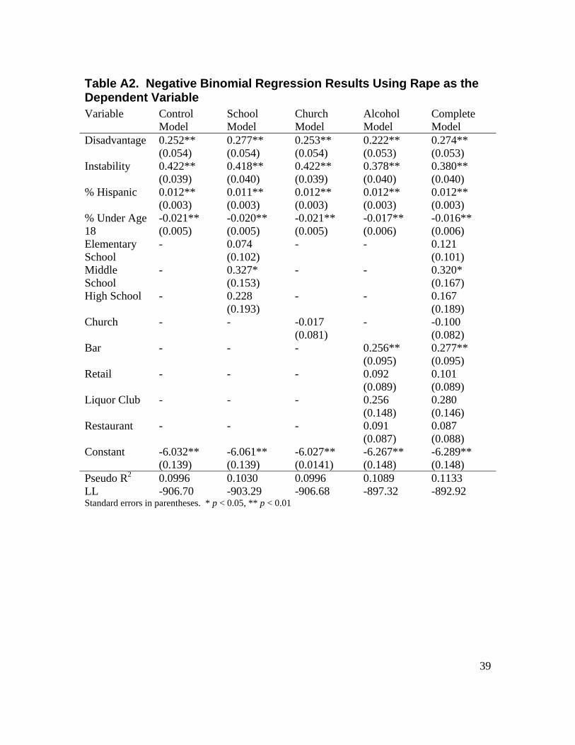
39

Table A2. Negative Binomial Regression Results Using Rape as the Dependent Variable Variable Control

Model School Model

Church Model

Alcohol Model

Complete Model

Disadvantage 0.252** (0.054)

0.277** (0.054)

0.253** (0.054)

0.222** (0.053)

0.274** (0.053)

Instability 0.422** (0.039)

0.418** (0.040)

0.422** (0.039)

0.378** (0.040)

0.380** (0.040)

% Hispanic 0.012** (0.003)

0.011** (0.003)

0.012** (0.003)

0.012** (0.003)

0.012** (0.003)

% Under Age 18

-0.021** (0.005)

-0.020** (0.005)

-0.021** (0.005)

-0.017** (0.006)

-0.016** (0.006)

Elementary School

- 0.074 (0.102)

- - 0.121 (0.101)

Middle School

- 0.327* (0.153)

- - 0.320* (0.167)

High School - 0.228 (0.193)

- - 0.167 (0.189)

Church - - -0.017 (0.081)

- -0.100 (0.082)

Bar - - - 0.256** (0.095)

0.277** (0.095)

Retail - - - 0.092 (0.089)

0.101 (0.089)

Liquor Club - - - 0.256 (0.148)

0.280 (0.146)

Restaurant - - - 0.091 (0.087)

0.087 (0.088)

Constant -6.032** (0.139)

-6.061** (0.139)

-6.027** (0.0141)

-6.267** (0.148)

-6.289** (0.148)

Pseudo R2 0.0996 0.1030 0.0996 0.1089 0.1133 LL -906.70 -903.29 -906.68 -897.32 -892.92 Standard errors in parentheses. * p < 0.05, ** p < 0.01

40

Table A3. Negative Binomial Regression Results Using Aggravated Assault as the Dependent Variable Variable Control

Model School Model

Church Model

Alcohol Model

Complete Model

Disadvantage 0.357** (0.040)

0.373** (0.040)

0.356** (0.040)

0.352** (0.035)

0.366** (0.035)

Instability 0.358** (0.029)

0.336** (0.029)

0.346** (0.029)

0.286** (0.026)

0.281** (0.026)

% Hispanic 0.011** (0.002)

0.011** (0.002)

0.011** (0.002)

0.011** (0.002)

0.011** (0.002)

% Under Age 18

-0.019** (0.004)

-0.019** (0.004)

-0.019** (0.004)

-0.016** (0.003)

-0.016** (0.003)

Elementary School

- -0.020 (0.069)

- - 0.050 (0.063)

Middle School

- 0.227* (0.111)

- - 0.196* (0.100)

High School - 0.357* (0.148)

- - 0.285* (0.133)

Church - - 0.059 (0.054)

- -0.032 (0.050)

Bar - - - 0.347** (0.060)

0.345** (0.061)

Retail - - - 0.246** (0.056)

0.247** (0.056)

Liquor Club - - - 0.160 (0.100)

0.162 (0.100)

Restaurant - - - 0.187** (0.055)

0.188** (0.056)

Lag 0.004** (0.001)

0.004** (0.001)

0.004** (0.001)

0.004** (0.001)

0.003** (0.001)

Constant -3.827** (0.094)

-3.841** (0.094)

-3.843** (0.095)

-4.082** (0.089)

-4.099** (0.089)

Pseudo R2 0.1102 0.1131 0.1105 0.1333 0.1359 LL -1780.41 -1774.45 -1779.80 -1734.16 -1728.91 Standard errors in parentheses. * p < 0.05, ** p < 0.01

41

Table A4. Negative Binomial Regression Results Using Robbery as the Dependent Variable Variable Control

Model School Model

Church Model

Alcohol Model

Complete Model

Disadvantage 0.327** (0.079)

0.340** (0.079)

0.325** (0.079)

0.388** (0.065)

0.395** (0.065)

Instability 0.276** (0.053)

0.263** (0.054)

0.274** (0.053)

0.141** (0.045)

0.139** (0.045)

% Hispanic 0.004 (0.003)

0.004 (0.003)

0.004 (0.003)

0.004 (0.003)

0.004 (0.003)

% Under Age 18

-0.024** (0.007)

-0.024** (0.007)

-0.024** (0.007)

-0.021** (0.006)

-0.021** (0.006)

Elementary School

- -0.019 (0.132)

- - 0.190 (0.108)

Middle School

- 0.232 (0.212)

- - 0.167 (0.175)

High School - 0.301) (0.281)

- - 0.138 (0.228)

Church - - 0.075 (0.100)

- -0.124 (0.086)

Bar - - - 0.709** (0.104)

0.734** (0.105)

Retail - - - 0.810** (0.095)

0.828** (0.094)

Liquor Club - - - 0.134 (0.172)

0.152 (0.171)

Restaurant - - - 0.573** (0.093)

0.585** (0.093)

Lag 0.035** (0.005)

0.036** (0.005)

0.035** (0.005)

0.026** (0.004)

0.027** (0.004)

Constant -4.750** (0.192)

-4.762** (0.192)

-4.779** (0.195)

-5.323** (0.154)

-5.351** (0.165)

Pseudo R2 0.0572 0.0581 0.0574 0.1117 0.1138 LL -1533.29 -1531.92 -1533.01 -1444.72 -1441.34 Standard errors in parentheses. * p < 0.05, ** p < 0.01

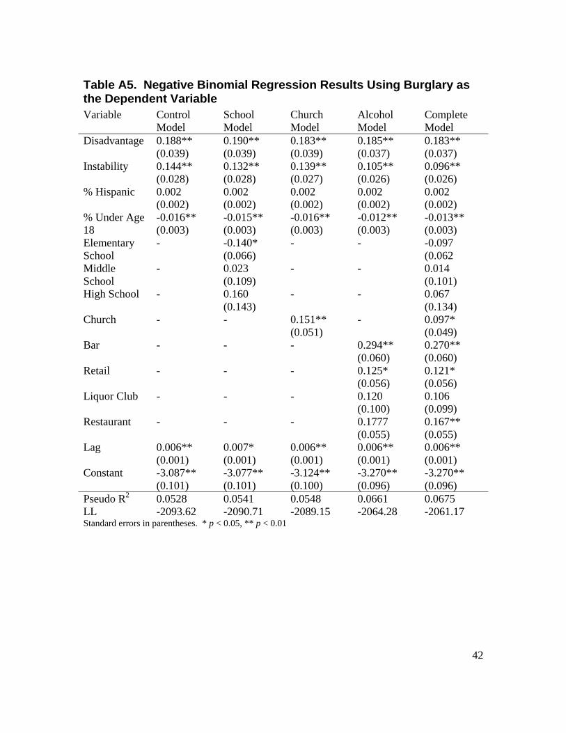
42

Table A5. Negative Binomial Regression Results Using Burglary as the Dependent Variable Variable Control

Model School Model

Church Model

Alcohol Model

Complete Model

Disadvantage 0.188** (0.039)

0.190** (0.039)

0.183** (0.039)

0.185** (0.037)

0.183** (0.037)

Instability 0.144** (0.028)

0.132** (0.028)

0.139** (0.027)

0.105** (0.026)

0.096** (0.026)

% Hispanic 0.002 (0.002)

0.002 (0.002)

0.002 (0.002)

0.002 (0.002)

0.002 (0.002)

% Under Age 18

-0.016** (0.003)

-0.015** (0.003)

-0.016** (0.003)

-0.012** (0.003)

-0.013** (0.003)

Elementary School

- -0.140* (0.066)

- - -0.097 (0.062

Middle School

- 0.023 (0.109)

- - 0.014 (0.101)

High School - 0.160 (0.143)

- - 0.067 (0.134)

Church - - 0.151** (0.051)

- 0.097* (0.049)

Bar - - - 0.294** (0.060)

0.270** (0.060)

Retail - - - 0.125* (0.056)

0.121* (0.056)

Liquor Club - - - 0.120 (0.100)

0.106 (0.099)

Restaurant - - - 0.1777 (0.055)

0.167** (0.055)

Lag 0.006** (0.001)

0.007* (0.001)

0.006** (0.001)

0.006** (0.001)

0.006** (0.001)

Constant -3.087** (0.101)

-3.077** (0.101)

-3.124** (0.100)

-3.270** (0.096)

-3.270** (0.096)

Pseudo R2 0.0528 0.0541 0.0548 0.0661 0.0675 LL -2093.62 -2090.71 -2089.15 -2064.28 -2061.17 Standard errors in parentheses. * p < 0.05, ** p < 0.01

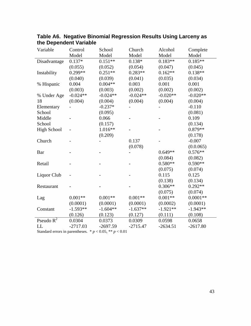
43

Table A6. Negative Binomial Regression Results Using Larceny as the Dependent Variable Variable Control

Model School Model

Church Model

Alcohol Model

Complete Model

Disadvantage 0.137* (0.055)

0.151** (0.052)

0.138* (0.054)

0.183** (0.047)

0.185** (0.045)

Instability 0.299** (0.040)

0.251** (0.039)

0.283** (0.041)

0.162** (0.035)

0.138** (0.034)

% Hispanic 0.004 (0.003)

0.004** (0.003)

0.003 (0.002)

0.001 (0.002)

0.001 (0.002)

% Under Age 18

-0.024** (0.004)

-0.024** (0.004)

-0.024** (0.004)

-0.020** (0.004)

-0.020** (0.004)

Elementary School

- -0.237* (0.095)

- - -0.110 (0.081)

Middle School

- 0.066 (0.157)

- - 0.109 (0.134)

High School - 1.016** (0.209)

- - 0.879** (0.178)

Church - - 0.137 (0.078)

- -0.007 (0.0.065)

Bar - - - 0.649** (0.084)

0.576** (0.082)

Retail - - - 0.580** (0.075)

0.590** (0.074)

Liquor Club - - - 0.115 (0.138)

0.125 (0.134)

Restaurant - - - 0.306** (0.075)

0.292** (0.074)

Lag 0.001** (0.0001)

0.001** (0.0001)

0.001** (0.0001)

0.001** (0.0002)

0.0001** (0.0001)

Constant -1.593** (0.126)

-1.604** (0.123)

-1.637** (0.127)

-1.921** (0.111)

-1.943** (0.108)

Pseudo R2 0.0304 0.0373 0.0309 0.0598 0.0658 LL -2717.03 -2697.59 -2715.47 -2634.51 -2617.80 Standard errors in parentheses. * p < 0.05, ** p < 0.01

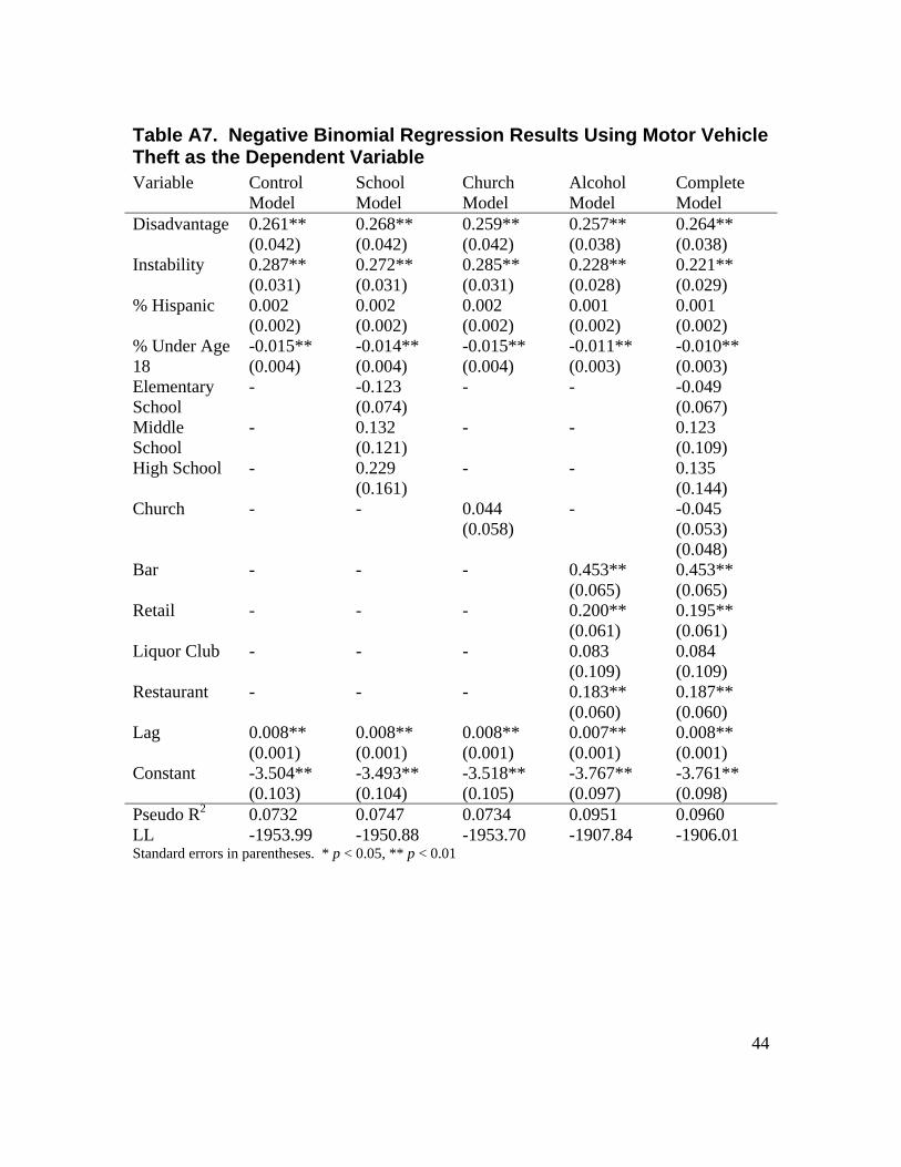
44

Table A7. Negative Binomial Regression Results Using Motor Vehicle Theft as the Dependent Variable Variable Control

Model School Model

Church Model

Alcohol Model

Complete Model

Disadvantage 0.261** (0.042)

0.268** (0.042)

0.259** (0.042)

0.257** (0.038)

0.264** (0.038)

Instability 0.287** (0.031)

0.272** (0.031)

0.285** (0.031)

0.228** (0.028)

0.221** (0.029)

% Hispanic 0.002 (0.002)

0.002 (0.002)

0.002 (0.002)

0.001 (0.002)

0.001 (0.002)

% Under Age 18

-0.015** (0.004)

-0.014** (0.004)

-0.015** (0.004)

-0.011** (0.003)

-0.010** (0.003)

Elementary School

- -0.123 (0.074)

- - -0.049 (0.067)

Middle School

- 0.132 (0.121)

- - 0.123 (0.109)

High School - 0.229 (0.161)

- - 0.135 (0.144)

Church - - 0.044 (0.058)

- -0.045 (0.053) (0.048)

Bar - - - 0.453** (0.065)

0.453** (0.065)

Retail - - - 0.200** (0.061)

0.195** (0.061)

Liquor Club - - - 0.083 (0.109)

0.084 (0.109)

Restaurant - - - 0.183** (0.060)

0.187** (0.060)

Lag 0.008** (0.001)

0.008** (0.001)

0.008** (0.001)

0.007** (0.001)

0.008** (0.001)

Constant -3.504** (0.103)

-3.493** (0.104)

-3.518** (0.105)

-3.767** (0.097)

-3.761** (0.098)

Pseudo R2 0.0732 0.0747 0.0734 0.0951 0.0960 LL -1953.99 -1950.88 -1953.70 -1907.84 -1906.01 Standard errors in parentheses. * p < 0.05, ** p < 0.01

45

Table A8. Negative Binomial Regression Results Using Narcotics Incidents as the Dependent Variable Variable Control

Model School Model

Church Model

Alcohol Model

Complete Model

Disadvantage 0.495** (0.070)

0.531** (0.063)

0.497** (0.070)

0.512** (0.065)

0.541** (0.057)

Instability 0.356** (0.049)

0.304** (0.045)

0.349** (0.050)

0.257** (0.047)

0.209** (0.041)

% Hispanic 0.011** (0.003)

0.012** (0.003)

0.011** (0.003)

0.010** (0.003)

0.010** (0.003)

% Under Age 18

-0.030** (0.005)

-0.030** (0.005)

-0.030** (0.005)

-0.028** (0.005)

-0.026** (0.005)

Elementary School

- 0.012 (0.105)

- - 0.092 (0.097)

Middle School

- 0.680** (0.170)

- - 0.799** (0.155)

High School - 1.564** (0.225)

- - 1.650** (0.203)

Church - - 0.097 (0.090)

- 0.032 (0.077)

Bar - - - 0.355** (0.108)

0.325** (0.096)

Retail - - - 0.349** (0.099)

0.407** (0.087)

Liquor Club - - - 0.492** (0.180)

0.536** (0.158)

Restaurant - - - 0.254** (0.095)

0.320** (0.086)

Lag 0.003** (0.001)

0.004** (0.001)

0.003** (0.001)

0.003** (0.001)

0.004** (0.001)

Constant -3.563** (0.146)

-3.799** (0.135)

-3.589** (0.148)

-3.846** (0.143)

-4.183** (0.129)

Pseudo R2 0.0732 0.0954 0.0735 0.0886 0.1182 LL -1882.91 -1837.74 -1882.34 -1851.52 -1791.56 Standard errors in parentheses. * p < 0.05, ** p < 0.01