Placement of Defect-Tolerant Digital Microﬂuidic Biochips ...cc.ee.ntu.edu.tw/~ywchang/Papers/jetc07-biochip.pdf · Placement of Defect-Tolerant Digital Microﬂuidic Biochips Using

13

Placement of Defect-Tolerant DigitalMicrofluidic Biochips Using theT-tree Formulation

PING-HUNG YUH, CHIA-LIN YANG, and YAO-WEN CHANG

National Taiwan University

Droplet-based microfluidic biochips have recently gained much attention and are expected to revo-lutionize the biological laboratory procedures. As biochips are adopted for the complex proceduresin molecular biology, its complexity is expected to increase due to the need of multiple and concur-rent assays on a chip. In this article, we formulate the placement problem of digital microfluidicbiochips with a tree-based topological representation, called T-tree. To the best knowledge of the au-thors, this is the first work that adopts a topological representation to solve the placement problemof digital microfluidic biochips. We also consider the defect tolerant issue to avoid to use defectivecells due to fabrication. Experimental results demonstrate that our approach is more efficient andeffective than the previous unified synthesis and placement framework.

Categories and Subject Descriptors: B.7.2 [Integrated Circuits]: Design Aids

General Terms: Algorithms, Performance, Design

Additional Key Words and Phrases: Microfluidics, biochip, placement

ACM Reference Format:Yuh, P.-H., Yang, C.-L., and Chang, Y.-W. 2007. Placement of defect-tolerant digital microflu-idic biochips using the T-tree formulation. ACM J. Emerg. Technol. Comput. Syst. 3, 3, Arti-cle 13 (November 2007), 32 pages. DOI = 10.1145/1295231.1295234 http://doi.acm.org/10.1145/1295231.1295234

This article is an extended and revised version of the paper presented at the 2006 IEEE/ACMDesign Automation Conference (DAC) C© ACM 2006.This work was partially supported by the National Science Council of Taiwan under Grant Nos. NSC95-2752-E-002-008-PAE and NSC 95-2221-E-002-374 and by the Excellent Research Projects ofNational Taiwan University, 95R0062-AE00-07.Authors’ address: P.-H. Yuh, C.-L. Yang (contact author), Department of CSIE, National TaiwanUniversity, No. 1, Sec. 4, Roosevelt Road, Taipei, Taiwan; email: {r91089, yangc}@csie.ntu.edu.tw;Y.-W. Chang, Graduate Institute of Electronics Engineering and Department of EE, NationalTaiwan University, No. 1, Sec. 4, Roosevelt Road, Taipei, Taiwan; email: [email protected] to make digital or hard copies of part or all of this work for personal or classroom use isgranted without fee provided that copies are not made or distributed for profit or direct commercialadvantage and that copies show this notice on the first page or initial screen of a display alongwith the full citation. Copyrights for components of this work owned by others than ACM must behonored. Abstracting with credit is permitted. To copy otherwise, to republish, to post on servers,to redistribute to lists, or to use any component of this work in other works requires prior specificpermission and/or a fee. Permissions may be requested from Publications Dept., ACM, Inc., 2 PennPlaza, Suite 701, New York, NY 10121-0701 USA, fax +1 (212) 869-0481, or [email protected]© 2007 ACM 1550-4832/2007/11-ART13 $5.00. DOI 10.1145/1295231.1295234 http://doi.acm.org/10.1145/1295231.1295234

ACM Journal on Emerging Technologies in Computing Systems, Vol. 3, No. 3, Article 13, Pub. date: November 2007.

13:2 • P.-H. Yuh et al.

1. INTRODUCTION

Due to the advances in the microfabrication and microelectromechanicalsystems, microfluidic technology has gained much attention recently. Thecomposite microsystems could perform conventional biological laboratory pro-cedures on a small and integrated system. As a result, microfluidic biochipsare used in several common procedures in molecular biology, such as the clinicdiagnosis and the DNA sequence analysis.

Most recently, second-generation (digital) microfluidic biochips, which arebased on the manipulation of the discrete liquid particles (the droplets), havebeen proposed [tutorgig]. Each droplet can be independently controlled by theelectrohydrodynamic forces generated by an electric field. The field can begenerated by an individually accessible electrode. Compared with the first-generation microfluidic biochips that are based on the continuous fluid flowand contain external pressure sources (e.g., micropumps), the droplets can bemoved anywhere in a 2D array to perform the desired chemical reaction and theelectrodes can be reprogrammed for different bioassays. With these two proper-ties, digital microfluidic biochips can handle large-scale and complex procedure,since the complex procedure can be built based on a set of fundamental oper-ations, such as droplet generation, mixing of multiple droplets, droplet trans-portation, droplet dilution, and droplet fission. Moreover, digital microfluidicbiochips can be reconfigured for different levels of hierarchy.

As biochips are adopted for complex procedures in molecular biology, thedesign complexity of digital microfluidic biochips is expected to increase dueto the need of multiple and concurrent assays on a biochip. The InternationalTechnology Roadmap for Semiconductors (ITRS) clearly points out that the in-tegration of electro-biological devices is one of the major challenges of systemintegration beyond 2009 [ITRS]. Besides, the increase in the density of as-says and area of digital microfluidic biochips may reduce yield. Since we needtime to ramp up the yield of biochips, it is desirable to perform a bioassayon a biochip with the existence of defects. How to incorporate the defect tol-erant issue in Computer Aided Design (CAD) support becomes an importantissue.

Figure 1 shows the schematic view of a digital microfluidic biochip basedon the principle of electrowetting on dielectric (EWOD) [Fair et al. 2003].There are three major components in a biochip: 2D microfluidic array, reser-voirs/dispensing ports, and optical detectors. The 2D microfluidic array consistsof a set of basic cells with the same architecture. The 2D microfluidic array isused for the chemical reaction of droplets and droplets transportation. With this2D array, fundamental microfluidic operations (e.g., mix, dilute, and store) canbe performed for different bioassays. The mix operation is to mix two dropletscontaining analytes and reagents. The two droplets route to the same locationand turn around some pivot points for fast mixing process. This operation canbe used for preprocessing, sample dilution, or reaction between samples andreagents. The dilution operation is to mix samples with buffers to reduce thesample concentration. The dilution ratio is controlled by a hierarchy of binarymixing phases by mixing samples (or diluted droplets) and buffers. The storage

ACM Journal on Emerging Technologies in Computing Systems, Vol. 3, No. 3, Article 13, Publ. date: November 2007.

Placement of Defect-Tolerant Digital Microfluidic Biochips • 13:3

Fig. 1. The schematic view of digital microfluidic biochips.

Fig. 2. An example of bioassay execution on digital microfluidic biochips.

operation is to temporarily preserve samples; that is, a droplet containing bio-logical sample is located at a fixed location for a period of time. Note that sincedroplets can move freely on the 2D array, these operations can be performedanywhere in this 2D array. In other words, a basic cell can perform differentoperations at different time steps. This property is referred to as the recon-figurability of biochips. Moreover, there are different implementations of theseoperations with different areas and durations. For example, a mix operation canbe performed in a 2×3 or 1×4 region with different mixing times. In this paper,we refer to this type of operations (mix, dilute) as the reconfigurable operations.The reservoirs/dispensing ports are responsible for droplets generation whilethe optical detectors are used for the detection of reaction results. In contrastto the 2D array, these devices have only one functionality. Therefore, in thispaper, we call these device as the non-reconfigurable devices. The operations(e.g., droplet dispensing/generation and detection) performed on these devicesare referred to as non-reconfigurable operations.

The bioassay is a procedure to determine the strength or activity of a bio-logical sample by comparing its effect with those standard preparations on theliving cells. Figure 2 shows the bioassay execution on a biochip. A bioassay isrepresented as a task graph, where each node represents a fundamental oper-ation and each edge represents the data dependency between two operations.Each fundamental operation (mix, dilution, etc.) occupies a certain area and


13:4 • P.-H. Yuh et al.

lasts for a period of time. There are two important characteristics of the execu-tion of a bioassay. First, due to the reconfigurability of biochips, two fundamen-tal operations may share the same area at different time steps. For example, themix operation b and the mix operation a share the same area. Second, a storageunit is required to temporarily store the intermediate result between two data-dependent fundamental operations. For example, although the mix operation ais finished at time 4, the mix operation c cannot immediately start its executionsince another input droplet of mix c is not available at that time. Therefore, astorage unit is required to store the result of the mix operation a. The above twocharacteristics complicates the placement of fundamental operations, since weneed to determine not only the physical location but also the starting time ofeach fundamental operation. Moreover, we also need to determine the numberof storages and the locations of them.

Due to the reconfigurability, the placement problem of digital microfluidicbiochips includes architectural-level synthesis (i.e., scheduling and resourcebinding) and physical placement. How to simultaneously perform architectural-level synthesis and physical placement is the most challenging issue in theplacement problem.

1.1 Related Works

Architectural-level synthesis and physical placement of digital microfluidicbiochips have been addressed in the recent literature. For the architectural-level synthesis, Ding et al. [2001] proposed an architectural-level modeling andan integer linear programming based optimization method for droplet-basedmicrofluidic biochips. Su et al. [Su and Chakrabarty 2004] used the sequencinggraph to represent the bioassay protocol and proposed an integer linear pro-gramming based formulation and two heuristics, the modified list schedulingalgorithm and the genetic algorithm, to solve this problem. Recently, Rickettset al. [2006] proposed the hybrid priority scheduling algorithm based on thegenetic algorithm. For the physical placement, Su et al. [Su and Chakrabarty2005a] proposed a simulated annealing-based algorithm for the physical place-ment problem with given scheduled operations. They also considered the faulttolerance issue by modeling the degree of faults and identifying the emptyspaces to recover operations with faulty cells. Recently, Su and Chakrabarty[2005b] presented a unified synthesis and placement flow based on parallelrecombinative simulated annealing. Their algorithm consisted of three stages:binding, scheduling, and physical placement. They used the list scheduling algo-rithm for scheduling and a greedy placement algorithm for physical placement.They also considered the defect tolerant issue for yield enhancement.

The synthesis and physical placement problem of digital microfluidicbiochips are closely related to the operations of dynamically reconfigurableFPGAs (DRFPGAs), which have received much attention recently [Bazarganet al. 2000]. The digital microfluidic biochips offers the same partial recon-figurability as the DRFPGAs. Many approaches, such as the graph-theoreticapproach [Fekete et al. 2001] and the topological representation based ap-proach [Yuh et al. 2004; Yuh et al. 2004], have been proposed. Among these



approaches, the T-tree [Yuh et al. 2004] representation is the state-of-the-artmethod for DRFPGAs.

1.2 Our Contribution

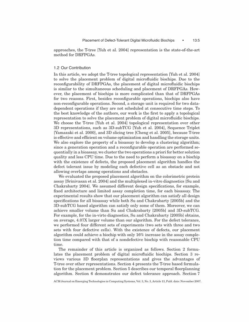
In this article, we adopt the T-tree topological representation [Yuh et al. 2004]to solve the placement problem of digital microfluidic biochips. Due to thereconfigurability of DRFPGAs, the placement of digital microfluidic biochipsis similar to the simultaneous scheduling and placement of DRFPGAs. How-ever, the placement of biochips is more complicated than that of DRFPGAsfor two reasons. First, besides reconfigurable operations, biochips also havenon-reconfigurable operations. Second, a storage unit is required for two data-dependent operations if they are not scheduled at consecutive time steps. Tothe best knowledge of the authors, our work is the first to apply a topologicalrepresentation to solve the placement problem of digital microfluidic biochips.We choose the T-tree [Yuh et al. 2004] topological representation over other3D representations, such as 3D-subTCG [Yuh et al. 2004], Sequence Triplet[Yamazaki et al. 2000], and 3D slicing tree [Cheng et al. 2005], because T-treeis effective and efficient on volume optimization and handling the storage units.We also explore the property of a bioassay to develop a clustering algorithm;since a generation operation and a reconfigurable operation are performed se-quentially in a bioassay, we cluster the two operations a priori for better solutionquality and less CPU time. Due to the need to perform a bioassay on a biochipwith the existence of defects, the proposed placement algorithm handles thedefect tolerant issue by modeling each defective cell as an obstacle and notallowing overlaps among operations and obstacles.

We evaluated the proposed placement algorithm on the colorimetric proteinassay [Srinivasan et al. 2004] and the multiplexed in-vitro diagnostics [Su andChakrabarty 2004]. We assumed different design specifications, for example,fixed architecture and limited assay completion time, for each bioassay. Theexperimental results show that our placement algorithm can satisfy all designspecifications for all bioassay while both Su and Chakrabarty [2005b] and the3D-subTCG based algorithm can satisfy only some of them. Moreover, we canachieve smaller volume than Su and Chakrabarty [2005b] and 3D-subTCG.For example, for the in-virto diagnostics, Su and Chakrabarty [2005b] obtains,on average, 4.07X larger volume than our algorithm. For the defect tolerance,we performed four different sets of experiments (two sets with three and twosets with four defective cells). With the existence of defects, our placementalgorithm could achieve a biochip with only 16% increase in the assay comple-tion time compared with that of a nondefective biochip with reasonable CPUtime.

The remainder of this article is organized as follows. Section 2 formu-lates the placement problem of digital microfluidic biochips. Section 3 re-views various 3D floorplan representations and gives the advantages ofT-tree over other representations. Section 4 presents the T-tree based formula-tion for the placement problem. Section 5 describes our temporal floorplanningalgorithm. Section 6 demonstrates our defect tolerance approach. Section 7


13:6 • P.-H. Yuh et al.

Fig. 3. Overview of the placement problem of biochips.

reports the experimental results. Finally, concluding remarks are given inSection 8.

2. PROBLEM FORMULATION

In this section, we give a formal definition about the placement problem ofdigital microfluidic biochips. Figure 3 shows the overview of the placementproblem. There are three inputs to the placement problem. The first one is thesequencing graph G = {V , E} that represents the protocol of a bioassay [Suand Chakrabarty 2004], where V = {v1, v2, . . . , vm} represents a set of m assayoperations and E = {(vi, vj ), 1 ≤ i, j ≤ m} denotes the data dependenciesbetween two assay operations; i.e., the precedence constraints. We may need atmost one storage unit for each edge in G to store the intermediate data betweentwo data-dependent operations. Throughout this paper, we use operation andtask interchangeably. The second one is the microfluidic module library thatcontains the basic modules for biochips. Each basic module is characterized byits functionality (i.e., mix, dilution, etc.) and parameters (i.e., width, height,and operation duration). The third one is the design specification, including:(1) the fixed architecture (such as 10 × 10 array) and limited assay completiontime (such as 400 seconds) and (2) the maximum number of instances for eachtype of non-reconfigurable devices; that is, the resource constraints.



Fig. 4. (a) A 3D placement. (b) Its corresponding 3D-subTCG.

The goal of our algorithm is to simultaneously perform resource binding,scheduling, and physical placement with volume optimization under the designspecification. Binding is to map an operation to a functional resource. Note thatthere may be several functional resources for a given operation. For example,for a reconfigurable operation, such as the mix operation, we can use a 2 × 2-array mixer or a 2×4-array mixer with different mixing times. However, severaloperations may map to the same functional resource for resource sharing. Forexample, we may map two detection operations to the same optical detector.After binding, the duration and dimension of each operation is determined.Scheduling is to determine the starting time of each operation under the prece-dence constraint. For a valid schedule, non-reconfigurable operations that mapto the same device cannot execute concurrently. Physical placement is to find thephysical location for each reconfigurable operation on the 2D microfluidic array.We also need to determine the locations of optical detectors. On the other hand,we can manually determine the reservoirs/dispensing ports after placement,since they do not affect the area of the biochip [Su and Chakrabarty 2005b].In this paper, we ignore the time for transporting droplets between differenttasks because the movement of droplets is very fast compared with the durationof each task [Fair et al. 2003; Srinivasan et al. 2004]. We also follow Su andChakrabarty [2005b] in using the segregation cells to wrap each reconfigurableoperation, storage unit, and optical detectors for not only providing the trans-portation path for droplets movement between different operations, but alsoisolating one operation from another to avoid unexpected cross-contamination.

3. REVIEW OF 3D FLOORPLAN REPRESENTATIONS

In this section, we briefly review popular 3D floorplan representations pro-posed in the recent literature, including 3D-subTCG [Yuh et al. 2004], SequenceTriplet (ST) [Yamazaki et al. 2000], T-tree [Yuh et al. 2004], and 3D slicingtree [Cheng et al. 2005]. Then we point out the advantages of T-tree over other3D representations.

3.1 3D-subTCG

3D-subTCG is an extension of the well-known 2D floorplan representation:Transitive Closure Graph (TCG) [Lin and Chang 2001]. 3D-subTCG uses ahorizontal transitive closure graph Ch and a vertical transitive closure graph Cv


13:8 • P.-H. Yuh et al.

t y

x

b

c

a

Fig. 5. A 3D floorplan; the corresponding Sequence Triplet is (bca, bac, abc).

to describe the geometric relations and a temporal transitive closure graph Ct

to model the temporal relations among tasks. Figure 4 shows a 3D placementand its corresponding 3D-subTCG. Each node ni in a transitive closure graphrepresents a task vi. The value associated with a node in Ch (Cv or Ct) gives thewidth (height or duration) of the corresponding task, and the edge (ni, nj ) in Ch

(Cv or Ct) represents the horizontal (vertical or temporal) relation of vi and vj .For example, in Figure 4, since task vc (va) is left to (below) vb (v f ), there existsan edge (nc, nb) ((na, n f )) in Ch (Cv). Similarly, since task va is executed beforetask vd , there exists an edge (na, nd ) in Ct .

3.2 Sequence Triplet

Sequence Triplet (ST) is a 3D representation extended from the well-knownSequence Pair representation [Murata et al. 1995]. An ST consists of threesequences (�1, �2, �3), where each sequence contains the label of all tasks.Figure 5 shows a simple 3D placement and its corresponding ST. ST defines therelations between two tasks based on the relative positions of this two tasks inthe three sequences. The relation between two tasks is defined as follows: (1) ifthe sequence of two tasks va, vb is the same (from left to right) in (�1, �2, �3), i.e.,(�1, �2, �3) = (..a..b.., ..a..b.., ..a..b..), it means that task vb is in the Y + directionof task va; (2) if (�1, �2, �3) = (..a..b.., ..a..b.., ..b..a..), it means that task vb is inthe X − direction of task va; (3) if (�1, �2, �3) = (..a..b.., ..b..a.., ..a..b..), it meansthat task vb is in the X + direction of task va; (4) if (�1, �2, �3) = (..a..b.., ..b..a..,..b..a..), it means that task vb is in the Z − direction of task va. For example,since the relative positions of tasks va and vb satisfy relation (2), va is in the X −

direction of vb.

3.3 T-tree

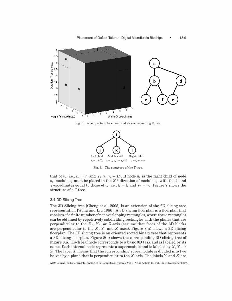
T-trees are a 3-ary tree, where each node corresponds to a unique task and hasat most three children to represent the dimensional relationship among tasks.The T-tree is designed to represent a compacted placement where each taskcannot move toward the origin. Figure 6 shows a compacted placement andits corresponding T-tree. Given a set of m tasks, let Wi, Hi, and Ti denote thewidth, height, and duration of each task, 1 ≤ i ≤ m. We use (xi, yi) ((i, y ′

i)) todenote the coordinate of the bottom-left (top-right) corner of a task vi, and ti

(t ′i ) the starting (ending) time of task vi, 1 ≤ i ≤ m. The T-tree represents the

geometric relationship between two tasks as follows. If node nj is the left childof node ni, module vj must be placed adjacent to module vi in the T+ direction,that is, t j = ti + Ti. If node nk is the middle child of node ni, module vk mustbe placed in the Y + direction of module vi, with the t-coordinate of vk equal to



Fig. 6. A compacted placement and its corresponding T-tree.

jj

ii

llkk

tj = ti + Ti tk = ti, yk >= yi+Hi tl = ti, yl = yi

Left child Right childMiddle child

Fig. 7. The structure of the T-tree.

that of vi, i.e., tk = ti and yk ≥ yi + Hi. If node nl is the right child of nodeni, module vl must be placed in the X + direction of module vi, with the t- andy-coordinates equal to those of vi, i.e., tl = ti and yl = yi. Figure 7 shows thestructure of a T-tree.

3.4 3D Slicing Tree

The 3D Slicing tree [Cheng et al. 2005] is an extension of the 2D slicing treerepresentation [Wong and Liu 1986]. A 3D slicing floorplan is a floorplan thatconsists of a finite number of nonoverlapping rectangles, where these rectanglescan be obtained by repetitively subdividing rectangles with the planes that areperpendicular to the X -, Y -, or Z -axis (assume that faces of the 3D blocksare perpendicular to the X , Y , and Z axes). Figure 8(a) shows a 3D slicingfloorplan. The 3D slicing tree is an oriented rooted binary tree that representsa 3D slicing floorplan. Figure 8(b) shows the corresponding 3D slicing tree ofFigure 8(a). Each leaf node corresponds to a basic 3D task and is labeled by itsname. Each internal node represents a supermodule and is labeled by X , Y , orZ . The label X means that the corresponding supermodule is divided into twohalves by a plane that is perpendicular to the X -axis. The labels Y and Z are


13:10 • P.-H. Yuh et al.

Fig. 8. (a) The 3D slicing structure. (b) The corresponding 3D slicing tree.

similarly defined. For example, the root of the two tasks v2 and v5 representsa supermodule. Since its label is Z , this supermodule is divided by the planethat is perpendicular to the Z -axis. Therefore, task v5 is in the Z + direction oftask v2.

3.5 Discussion

In this section, we give the advantages of the T-tree over the other represen-tations for the placement problem of digital microfluidic biochips, for which wechoose the T-tree representation to solve the problem addressed in this paper:

(1) T-tree models compacted floorplans whose modules are compacted towardthe origin, while the 3D-subTCG and ST model general floorplans and the3D slicing tree models slicing floorplans. Recall that for the placement prob-lem of digital microfluidic biochips, we need to satisfy the given fixed archi-tecture and limited assay completion time. Therefore, a feasible 3D floor-plan must be within the 3D cube defined by the fixed architecture andlimited assay completion time. Since the T-tree models a compacted floor-plan, it is more suitable for volume optimization, and thereby is more likelyto generate solutions that are within the defined 3D cube. Consequently,T-tree is more suitable for the placement problem of digital microfluidicbiochips than other 3D representations.

(2) Recall that we need a storage unit for two data-dependent operations ifthey are not scheduled at consecutive time steps. Also, the number andduration of these storage units are related to the schedule of operations.Based on the structure of T-tree, we can easily determine the number ofstorage units and their duration before packing. This process takes onlylinear time. As for 3D-subTCG and ST, we need, on average, O(m2) timeto obtain this information with m operations since each transitive closuregraph has average m(m−1)

6 edges. For the 3D slicing tree, this informationcannot be obtained before packing. Further, the number of storage unitsvaries with different schedules. We may need to delete an unused storageunit or insert a new one during simulated annealing (SA) for packing ef-ficiency. For 3D-subTCG, when deleting an unused storage unit (insertinga new storage unit), we need to delete (insert) an edge from this storageunit to all other tasks, and detect whether the properties of 3D-subTCG aresatisfied after deletion (insertion). That is, we need to detect whether the



transitive closure property is satisfied and there exists no cycles in eachtransitive closure graph. We need O(|E|) time to detect cycles and to main-tain the transitive closure property for inserting/deleting one edge, whereE is the set of edges in one transitive closure graph. For ST, we need todetermine the positions of a storage unit in (�1, �2, �3) for insertion, sincewe need to satisfy the requirement of storage units—a storage operation vs

must be performed after the finish of vi if vs stores the result of vi. This pro-cess may need O(km) time, where k is the number of storage units requiredfor insertion. For the 3D slicing tree, it is hard to guarantee that the dura-tion of one storage unit equals the time gap between two data-dependentoperations. Therefore, it is harder for a 3D slicing tree to obtain a feasiblesolution.

(3) As described in Section 1, the size (number of operations) of a bioassayis expected to increase because the design of a biochip will become morecomplicated to handle concurrent assays on a chip. Therefore, the efficiencyof handling large-scale bioassays is one important factor when evaluatingthe suitability of a 3D representation for the placement problem of biochips.It has been shown [Yuh et al. 2004] that T-tree is more efficient and effectivethan 3D-subTCG and ST for the simultaneous scheduling and placementproblem of DRFPGAs. Since the problem addressed here is closely relatedto that of the DRFPGAs, we expect the T-tree to also be more efficient andeffective than 3D-subTCG and ST.

With these reasons, we decide to choose the T-tree representation to handlethe placement problem of digital microfluidic biochips.

4. T-TREE BASED BIOCHIP PLACEMENT

In this section, we first present the challenges of solving the placement problemof biochips. Then we demonstrate that the execution of tasks on a biochip canbe modeled as the temporal floorplanning problem. Finally, we present how tomodel each type of tasks with the T-tree formulation and how to handle thedesign specification in our algorithm.

Due to the reconfigurability of both DRFPGAs and biochips, the placementof digital microfluidic biochips is similar to the simultaneous scheduling andplacement of DRFPGAs. At first glance, one may apply the techniques for DRF-PGAs to solve the placement problem of biochips. However, the placement ofbiochips is more complicated than that of DRFPGAs based on the following tworeasons.

(1) In addition to reconfigurable operations, biochips also have non-reconfigurable operations. These non-reconfigurable operations have dif-ferent characteristics from that of reconfigurable operations. For example,since droplets are generated at the reservoirs/dispensing ports which areon the boundary of the 2D microfluidic array, the generation operations donot occupy the area of the 2D microfluidic array. Another example is thedetection operations. Since the detectors are fixed after fabrication, two de-tection operations using the same detector must have the same physical


13:12 • P.-H. Yuh et al.

Fig. 9. The two placements with the same biochip area and number of reconfigurable operationsbut with different number of storage units.

location in the 2D microfluidic array. Besides, the total number of non-reconfigurable operations at any time is limited due to the limited numberof non-reconfigurable devices. As a result, we require different ways to han-dle these non-reconfigurable operations.

(2) In digital microfluidic biochips, a storage unit is required for two data-dependent operations if they are not scheduled at consecutive time steps.The existence of the storage units complicates the placement problem fortwo reasons. First, instead of only area estimation as used in Su andChakrabarty [2004], we need detail physical information of these storageunits for accurate biochip area calculation. We use Figure 9 as an exampleto illustrate this scenario. Figure 9 shows two placements with the samebiochip area (10 × 10) and the same number of reconfigurable operations(5 operations). Note that for the purpose of functional isolation and droplettransportation, we use the segregation cells to wrap each operation andstorage unit. Although these two placements have the same biochip area,they differ in the number of storage units. If no detail physical informationof the storage units is provided, we cannot obtain the exact biochip area.We may conclude that the area of Figure 9(a) is larger than that of Fig-ure 9(b), since the number of storage units of Figure 9(a) is larger than thatof Figure 9(b) if only area estimation of storage units is used.Second, the number and duration of the storage units are not determined apriori. More importantly, the number and duration of the storage units arerelated to current schedule of operations. This characteristic makes storageunits different from modules in traditional temporal floorplanning problem,where the number of modules and the volume of each module are inputs andremain unchanged during floorplanning. We use Figure 10 as an exampleto explain this characteristic. In this figure, we model each operation as a3D box. Figure 10 shows a bioassay with two data-dependent operations.For each operation and storage unit, we model it as a 3D box. As shown inFigure 10(a), since operation vb starts right after operation va finishes, we donot need a storage unit. Figure 10(b) shows its corresponding 3D placementwith two operations. Now suppose that vb starts one time unit after va



Fig. 10. Examples to show the characteristics of storage units. (a) Two tasks on a biochip. (b)The corresponding 3D floorplan of (a). (c) Two tasks with a storage unit. (d) The corresponding 3Dfloorplan of (c). Note that we have three modules in this floorplan. (e) Two tasks with a storageunit. (f) The corresponding 3D floorplan of (e). The duration of the storage unit is increased from 1to 2 time units.

finishes, as shown in Figure 10(c). In this situation, we need one storageunit to store the intermediate result between vb and va. Figure 10(d) showsits corresponding 3D placement. Note that compared with the 3D placementshown in Figure 10(b), we now have three modules corresponding to twooperations and one storage unit vs. Therefore, the number of storage unitsis related to the schedule of the data-dependent operations. Figure 10(e)shows another scenario, where vb starts two time units after va finishes.Figure 10(f) shows the corresponding 3D placement. Compared with the 3Dplacement shown in Figure 10(d), the duration of vs is increased from onetime unit to two time units. This is because the duration of vs must cover thetime difference between va and vb. As a result, the duration of storage unitsis also related to the schedule of two data-dependent operations. Anotherobservation from Figure 10 is that the starting time of vs is equal to theending time of va and the ending time of vs is the same as the startingtime of vb, as shown in Figures 10(d) and (f). We need to satisfy the aboverequirements of storage units when solving the placement problem.

Now we present our T-tree based placement formulation. Due to the recon-figurability of biochips, the execution of a set of tasks can be viewed as a 3Dfloorplan as shown in Figure 11. The X and Y dimensions give the area of a


13:14 • P.-H. Yuh et al.

Fig. 11. (a) Two operations are executed at time t1. (b) At time t2, operation 3 starts to executeat the same physical location as operation 2. (c) The 3D modeling of the execution of the threeoperations.

biochip while the T dimension represents the duration of a bioassay. Supposethat both operations v1 and v2 are executed at time t1, as shown in Figure 11(a).Figure 11(b) shows that at time t2, we can perform operation v3 at the samephysical location as operation v3 after operation v2 is finished. The execution ofthe three operations can be modeled as a set of 3D modules with their widthsand heights (X and Y dimensions) representing the physical dimensions occu-pied by the operations in a biochip and its duration (T dimension) being theexecution time required for operations, as shown in Figure 11(c). Since the ex-ecution of a set of operations can be mapped to a 3D floorplan, we can applythe temporal floorplanning techniques to solve the placement problem of digitalmicrofluidic biochips.

For each task in a sequencing graph, we create a unique node in a T-tree. Notethat there are both reconfigurable and non-reconfigurable tasks in a biochip.For reconfigurable tasks and detection tasks, since we need to perform thistype of tasks in the 2D microfluidic array, we model it as a 3D box. For non-reconfigurable tasks except the detection tasks, since the reservoirs and dis-pensing ports are outside the 2D microfluidic array as shown in Figure 1, weneed only to consider the time aspect for this type of tasks. Therefore, we modelit as a 3D line with both its width and height being zero.

In this paragraph, we describe how we model the storage units. We create anode ns for each storage unit vs. Since vs holds the intermediate data betweentwo data-dependent tasks vi and vj , vs must satisfy the storage constraint. Thestorage constraint states that the starting time of vs must be equal to the endingtime of vi and the ending time of vs must be equal to the starting time of vj .Figure 12 illustrates how to find the feasible locations for ns in a T-tree to satisfythe storage constraint. Suppose that we want to find the feasible locations forns. Recall that if nj is the left child of ni, the starting time of vj is the sameas the ending time of vi. Otherwise, the starting time of vj is the same as thestarting time of vi. Thus, based on the structure of T-tree, the starting time ofvc in Figure 12 is the same as the ending time of va, and the starting times of



Fig. 12. An example of finding the feasible locations for a storage unit in a T-tree. Suppose thattasks va and vb need a storage unit vs.

vb, vc, and vd are the same. Based on above observation, the feasible locationsof ns are the middle or the right child of nodes nb, nc, or nd , as the black boxesshown in Figure 12. After placing ns in its feasible location, we set the endingtime of vs as the starting time of vb. Note that the duration of vs is not fixed; itvaries based on the starting time of vb.

The design specification describes the fixed architecture, the limited assaycompletion time, and the resource constraints. We model the fixed architec-ture and limited assay completion time as the fixed-cube constraint. The fixed-cube constraint states that a feasible 3D floorplan must be within a 3D cube.To handle the resource constraints, we introduce the concept of the virtualprecedence constraints. If two non-reconfigurable tasks are bound to the samenon-reconfigurable resource, such as the same dispensing port, these two non-reconfigurable tasks cannot be executed at the same time. Therefore, we addan additional edge between these two tasks in the sequencing graph to satisfythe resource constraint. Note that there is no storage unit requirement in theseadditional edges.

5. THE FLOORPLANNING ALGORITHM

Our algorithm is based on the simulated annealing (SA) method [Kirkpatricket al. 1983]. We adopt SA instead of genetic algorithm (GA) as our optimizationmethod because it has been shown that SA is typically more efficient and eco-nomical than GA for the problems in electronic design automation (EDA). GAneeds to maintain a set of solutions, called the population. At each iteration, GAneeds to evaluate the fitness function for each solution in the current popula-tion. On the other hand, SA maintains only two solutions—the current solutionand the best one. At each iteration, SA needs only to evaluate the current so-lution. As a result, SA typically needs less CPU time than GA. Moreover, SAuses less memory than GA due to the smaller number of solutions maintained.

Before performing SA, we first cluster one generation operation with onereconfigurable operation to reduce the CPU time and to increase the chanceof obtaining more compact 3D floorplans. During SA, given a feasible T-tree,we perturb it to obtain another feasible T-tree through a set of predefined SAoperations. After perturbation, we perform a feasibility detection and tree re-construction process to obtain a feasible topology with respect to the precedence


13:16 • P.-H. Yuh et al.

a b

c d

e f

g

ih

j k

l m

T

operationf

Operationk

Stor-ageunit

(a)

(b)

X

Operationj

T

operationf

Operationk

(c)

X

Operationj

Generation

ReconfigurableOperation

Detection

Fig. 13. (a) A sample sequencing graph. (b) A partial floorplan with v f being scheduled long beforevk starts. (c) Another partial floorplan with v f being scheduled right before vk starts.

constraints and the storage constraints. Finally, a packing procedure that placesall operations and optical detectors is invoked to evaluate the solution quality.

5.1 Clustering of Generation and Reconfigurable Operations

In this section, we detail our clustering algorithm. The goal of the clustering al-gorithm is to obtain a more compact 3D floorplan and to reduce the CPU time byreducing unnecessary storage units. This clustering algorithm is motivated bytwo observations. First, a generation operation and a reconfigurable operationare always performed in sequence, since we need to first generate a droplet andthen to perform reactions. Second, we may improve the solution quality (e.g.,volume) and reduce the CPU time by reducing the amount of storage units re-quired via clustering. Recall that we need a storage unit for two data-dependenttasks if they are not scheduled at consecutive time steps. The duration of thisstorage unit also varies based on the starting and ending times of these twotasks. Since the storage units occupy certain volumes, the number and dura-tion of them have great effect on the total volume of a 3D floorplan. If we canminimize the volume of these storage units, we may obtain a more compact 3Dfloorplan. We use the sample sequencing graph shown in Figure 13(a) as anexample. Figure 13(b) shows a partial floorplan. For simplicity, we only showthe X and T dimensions.1 In this floorplan, since task v f finishes much earlierthan task vk starts, the storage unit vs will have a very long duration. Therefore,we may obtain a less compact 3D floorplan due to the non-overlapping require-ment among vs and other tasks. On the other hand, Figure 13(c) shows another

1For illustration purpose, in this figure, the width of the generation operation v f is not zero.



partial floorplan. In this floorplan, since v f finishes right before vk starts, we donot need a storage unit between v f and vk . By scheduling a generation opera-tion as near as its data-dependent reconfigurable operation, we can effectivelyminimize the unnecessary volume occupied by a storage unit. In this way, wehave a higher chance to obtain a 3D floorplan with smaller area.

The idea of the proposed clustering algorithm is that: given a sequencinggraph G, we randomly cluster one generation operation vg with one reconfig-urable operation vr if there exist an edge between vg and vr in G. After cluster-ing, the ending time of vg is the same as the starting time of vr . By this method,we do not need the storage unit between vg and vr . The other advantage is thatwe can reduce the number of nodes in a T-tree to speed up the packing pro-cess. However, one disadvantage is that we may potentially increase the assaycompletion time. The reason is as follows. Recall that we assign virtual prece-dence constraints among tasks that are bound to the same non-reconfigurabledevice. Suppose that there exists a virtual precedence constraint between twogeneration operations vg and vq . If we cluster vg and vr , we merge vg and vr

into a new task vl . So now we have a virtual precedence constraint between vl

and vq . This means that vq starts after vl finishes rather than after vg finishes.Therefore, the assay completion time is potentially increased due to clustering.In order not to increase the assay completion time, we do not actually clustervg and vr into a new task. In our current implementation, we add additionalrequirement on nodes ng and nr in a T-tree. We require that nr will always bethe left child of ng in a T-tree. This requirement has the same effect as clus-tering two tasks, since the ending time of vg is the same as the starting timeof vr if nr is the left child of ng . In our floorplanning algorithm, if we performSA operation on ng , we also perform the same SA operation on nr . We alsocheck if the two clustered nodes are in their correct positions in a T-tree duringfeasibility detection and tree reconstruction process, which will be presented inSection 5.5.

5.2 Perturbation

The original SA operations defined in Yuh et al. [2004] contain Move, Swap,and Rotation. For the placement of digital microfluidic biochips, we introducea new type of SA operations, called Rebind. Rebind is to bind a task to anotherfunctional resource. For a reconfigurable task, such as the mix operation, werandomly select a resource instance for this task. For example, we can changefrom a 2 × 2-array mixer to a 2 × 4-array mixer with different mixing times.For a non-reconfigurable task, we randomly change a task from one instance toanother. For example, suppose that we have two optical detectors p1 and p2 fordetection operations. For a detection operation vd that originally uses p1, wecan rebind it to p2. Note that since we add the virtual precedence constraintsamong tasks corresponding to the same non-reconfigurable resource instance,we modify these virtual precedence constraints after rebinding. For instance,when we bind vd from p1 to p2, we delete all virtual precedence constraints ofvd and add the virtual precedence constraints between all other tasks that arebound to p2 and vd .


13:18 • P.-H. Yuh et al.

We now show how to add the virtual precedence constraints between tasksthat are bound to the same non-reconfigurable device when performing theRebind SA operation. We add the virtual precedence constraints among tasksbound to the same non-reconfigurable device based on the execution level, orlv(i), of each operation vi. The intuition is that if lv(i) is larger than lv( j ),then operation vi is executed before operation vj . We add a virtual precedenceconstraint from vi to vj if lv(i) is larger than lv( j ). Given a sequencing graph G,we can recursively calculate lv(i) for each task vi in G. We first assign lv(i) = 0for all tasks vi with zero out-degree in G. For example, in Figure 13(a), lv(l ) andlv(m) are both zero. We then delete all assigned tasks and assign lv(i) = 1 for allremaining tasks with zero out-degree in G. For example, in Figure 13(a), lv( j )and lv(k) are both one. The above process repeats until all tasks are assignedits execution level.

We also enhance the original SA operations to handle the fixed-cube con-straint. We bias the Move operation based on the probability of violating thefixed-cube constraint in each dimension. Let kw (kh, kt) be the number of floor-plans whose width (height, completion time) exceeds the user-specified width(height, completion time) in the last r iterations. In this paper, we set r equal500. We bias the selection of the destination of the Move operation based on thevalues kw/r, kh/r, and kt/r. For example, a larger kw/r implies that it is moredifficult to fit the floorplans to the 3D cube in the X direction. Therefore, weshould try to place tasks along the Y or T directions to satisfy the fixed-cubeconstraint.

5.3 Placement of Optical Detectors

In this section, we describe how to place the optical detectors in our algo-rithm. After the chemical reaction among droplets, we need optical detectorsto detect the reaction results. We need to determine the locations of theseoptical detectors during floorplanning. These detectors are fixed after fabri-cation. Therefore, if two detection operations map to the same optical detec-tor, they should be placed at the same physical location. Note that the seg-regation cells are also needed for the optical detectors to avoid the opticalinterference.

Suppose that two detection operations vi and vj are bound to the same op-tical detector and we first determine the location of vi. The basic idea is thatwe simultaneously determine the locations of vi and vj . Once the locations of vi

and vj are determined, the location of the optical detector is also determined.Note that when placing the detection operations, we also warp these operationswith the segregation cells. By this method, we can guarantee that the opticaldetectors are warped with the segregation cells after floorplanning. After de-termining the location of vi, we set vj at the same location as vi. The originalpacking algorithm of T-tree maintains a list L to store all tasks whose locationsare already determined [Yuh et al. 2004]. Finally, we add vj into L to indicatethat the location of vj is already determined. Note that we need to check if vj

overlaps with any other tasks in L. If vj overlaps with some tasks, we shift bothvi and vj along the X direction to avoid the overlap.



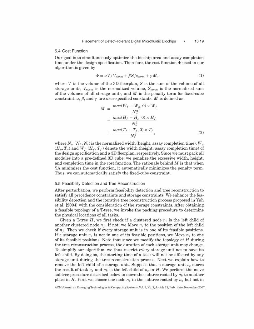
5.4 Cost Function

Our goal is to simultaneously optimize the biochip area and assay completiontime under the design specification. Therefore, the cost function � used in ouralgorithm is given by

� = αV/Vnorm + βS/snorm + γ M , (1)

where V is the volume of the 3D floorplan, S is the sum of the volume of allstorage units, Vnorm is the normalized volume, Snorm is the normalized sumof the volumes of all storage units, and M is the penalty term for fixed-cubeconstraint. α, β, and γ are user-specified constants. M is defined as

M = max(W f − Wp, 0) × W f

N 2w

+ max(Hf − Hp, 0) × Hf

N 2h

+ max(Tf − Tp, 0) × Tf

N 2t

, (2)

where Nw (Nh, Nt) is the normalized width (height, assay completion time), Wp

(Hp, Tp) and W f (Hf , Tf ) denote the width (height, assay completion time) ofthe design specification and a 3D floorplan, respectively. Since we must pack allmodules into a pre-defined 3D cube, we penalize the excessive width, height,and completion time in the cost function. The rationale behind M is that whenSA minimizes the cost function, it automatically minimizes the penalty term.Thus, we can automatically satisfy the fixed-cube constraint.

5.5 Feasibility Detection and Tree Reconstruction

After perturbation, we perform feasibility detection and tree reconstruction tosatisfy all precedence constraints and storage constraints. We enhance the fea-sibility detection and the iterative tree reconstruction process proposed in Yuhet al. [2004] with the consideration of the storage constraints. After obtaininga feasible topology of a T-tree, we invoke the packing procedure to determinethe physical locations of all tasks.

Given a T-tree H, we first check if a clustered node ni is the left child ofanother clustered node nj . If not, we Move ni to the position of the left childof nj . Then we check if every storage unit is in one of its feasible positions.If a storage unit ns is not in one of its feasible positions, we Move ns to oneof its feasible positions. Note that since we modify the topology of H duringthe tree reconstruction process, the duration of each storage unit may change.To simplify our algorithm, we thus restrict every storage unit not to have itsleft child. By doing so, the starting time of a task will not be affected by anystorage unit during the tree reconstruction process. Next we explain how toremove the left child of a storage unit. Suppose that a storage unit vs storesthe result of task va and nk is the left child of ns in H. We perform the movesubtree procedure described below to move the subtree rooted by nk to anotherplace in H. First we choose one node nz in the subtree rooted by na but not in


13:20 • P.-H. Yuh et al.

ss

kk

pp

zz

bb cc dd

(a) (b)

aa

ss

kk

pp

zz

bb cc

aa

dd

Fig. 14. The example of moving a subtree rooted by nk as the left subtree of nz . (a) A T-tree beforemoving the subtree rooted by nk . (b) A T-tree after moving the subtree rooted by nk as the leftsubtree of nz .

the subtree rooted by nk . Then we randomly move the subtree rooted by nk tothe positions of the left subtree, middle subtree, or right subtree of nz based onthe values of kw/r, kh/r, and kt/r defined in Section 5.2. For example, if kt/ris large, then we have lower probability to move the subtree rooted by nk tothe position of the left subtree of nz . Without loss of generality, assume that wemove the subtree rooted by nk to the position of the left subtree of nz . The othertwo cases can be handled similarly. First, if nz has no left child, then we cansimply move the subtree rooted by nk to the position of the left subtree of nz .Second, if nz has its left child, we need to consider two situations:

(1) nk has its left child: In this case, we first move the subtree rooted by nz ’sleft child to the position of the left subtree of nk . Then we move the subtreeoriginally rooted by nk ’s left child to the position of the left subtree of n f ,where n f is in the subtree rooted by nk with no left child.

(2) nk has no left child: In this case, we can simply move the subtree rooted bynz ’s left child to the position of the left subtree of nk .

Figure 14 gives an example if we move the subtree rooted by nk to the positionof the left subtree of nz . Figure 15 summaries the move subtree procedure.

Once all storage units are in their feasible positions and do not have theirleft child, we traverse H to obtain the starting time of each task. Next, we checkthe precedence constraints and reconstruct H if necessary based on the methodproposed in Yuh et al. [2004]. The main loop terminates when the topology ofH is not changed, which means that all precedence constraints and storageconstraints are satisfied. Then we assign the duration of each storage unit andadjust the number of storage units by deleting an unused storage unit and/orinserting a new one.

Note that we need to satisfy all precedence constraints after deleting orinserting a storage unit. It is easy to observe that inserting a new storageunit into one of its feasible positions does not affect the starting time of otheroperations. Thus, we do not violate the precedence constraints after insertion.However, deleting a storage unit with the Deletion SA operation presented



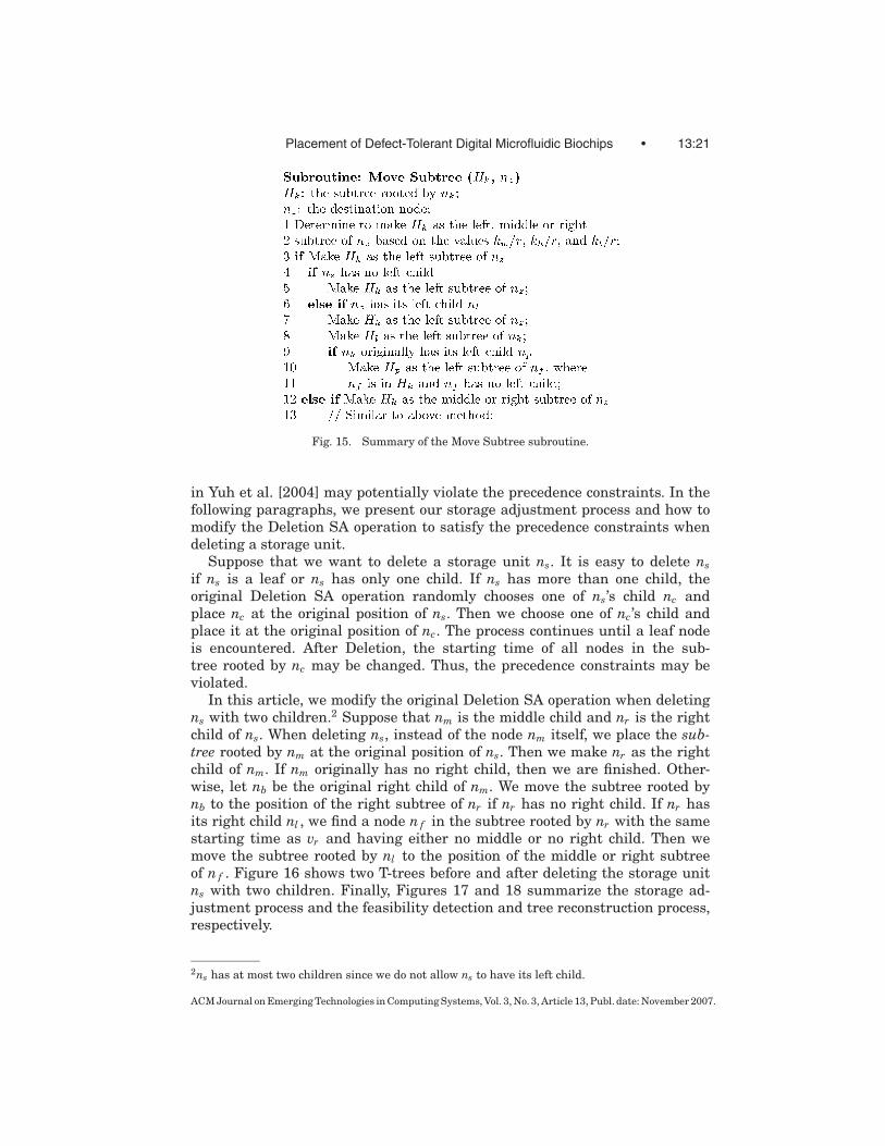
Fig. 15. Summary of the Move Subtree subroutine.

in Yuh et al. [2004] may potentially violate the precedence constraints. In thefollowing paragraphs, we present our storage adjustment process and how tomodify the Deletion SA operation to satisfy the precedence constraints whendeleting a storage unit.

Suppose that we want to delete a storage unit ns. It is easy to delete ns

if ns is a leaf or ns has only one child. If ns has more than one child, theoriginal Deletion SA operation randomly chooses one of ns’s child nc andplace nc at the original position of ns. Then we choose one of nc ’s child andplace it at the original position of nc. The process continues until a leaf nodeis encountered. After Deletion, the starting time of all nodes in the sub-tree rooted by nc may be changed. Thus, the precedence constraints may beviolated.

In this article, we modify the original Deletion SA operation when deletingns with two children.2 Suppose that nm is the middle child and nr is the rightchild of ns. When deleting ns, instead of the node nm itself, we place the sub-tree rooted by nm at the original position of ns. Then we make nr as the rightchild of nm. If nm originally has no right child, then we are finished. Other-wise, let nb be the original right child of nm. We move the subtree rooted bynb to the position of the right subtree of nr if nr has no right child. If nr hasits right child nl , we find a node n f in the subtree rooted by nr with the samestarting time as vr and having either no middle or no right child. Then wemove the subtree rooted by nl to the position of the middle or right subtreeof n f . Figure 16 shows two T-trees before and after deleting the storage unitns with two children. Finally, Figures 17 and 18 summarize the storage ad-justment process and the feasibility detection and tree reconstruction process,respectively.

2ns has at most two children since we do not allow ns to have its left child.


13:22 • P.-H. Yuh et al.

ss

mm

zz

rr

aa bb ll

mm

aa

zz

rr

ll

bb

(a) (b)

Fig. 16. The example of deleting a storage unit ns. (a) A T-tree before deleting ns (b) A T-tree afterdeleting ns.

Fig. 17. Summary of the storage adjustment process.

6. DEFECT TOLERANCE

In this section, we show how to extend the aforementioned temporal floorplan-ning algorithm to handle the defect tolerant issue. With the standard micro-fabrication techniques [Fair et al. 2003] and the synthesis result, a digital mi-crofluidic biochip can be fabricated. However, due to the underlying mixingtechnology, the microfluidic biochips have unique defects and failure mech-anism [Su et al. 2006]. The reconfigurability of the biochips can bypass the



Fig. 18. Summary of the feasibility detection and tree reconstruction process.

defective cells to tolerate the defects due to fabrication. Moreover, the non-reconfigurable device, such as the detectors, may be unavailable due to theexistence of the defects. We need to rebind the operations from an unavailabledetector to other available detectors. Note that after fabrication, the locations ofthe non-reconfigurable devices are fixed. We cannot move these detectors duringfloorplanning.

The central idea of our algorithm is that we model each defective cell as anobstacle. If a cell c located at (x, y) becomes faulty, we create an obstacle dc

located at (x, y) with its duration being the same as the assay completion time.In the packing process, we do not allow the overlap among tasks and obstacles.By this method, we can guarantee that no task will overlap with obstacle dc,and thereby avoid to place tasks on defective cells.

We now present our obstacle avoidance algorithm to avoid overlaps amongreconfigurable operations and obstacles. As mentioned above, we create an ob-stacle for each defective cell. During the packing process, we detect if a task vi

overlaps with any obstacle dc. If vi overlaps with an obstacle dc, we first calcu-late the X-span sx and Y-span sy . The X-span (Y-span) represents how far weshould shift vi along the X (Y ) direction to avoid the overlap with dc. In thispaper, we set sx (sy ) as the difference between x ′

c and xi ( y ′c and yi), where (x ′

c,y ′

c) is the up-right coordinate of dc. We shift vi along the direction that resultsin smaller movement distance. That is, if sx < sy , we shift vi in the X direction;otherwise, we shift vi in the Y direction. Figure 19 summaries our obstacleavoidance process.


13:24 • P.-H. Yuh et al.

Fig. 19. Summary of the obstacle avoidance algorithm.

Fig. 20. The sequencing graph of colorimetric protein assay [Su and Chakrabarty 2005b].

7. EXPERIMENTAL RESULTS

Our algorithm was implemented in the C++ programming language and run ona 1.066 GHz SUN Blade 1500 machine with 4 GB memory. We implemented theunified synthesis and placement algorithm proposed in Su and Chakrabarty[2005b] and the 3D-subTCG representation on the same machine. For 3D-subTCG, we used the same SA engine as T-tree. We modified the operationsof 3D-subTCG to satisfy the storage constraint at each perturbation. We alsoapplied the clustering algorithm proposed in Section 5.1 to 3D-subTCG for faircomparison. For all experiments, we set α = 1

21.5 , β = 0.521.5 , and γ = 20

21.5 . We alsoassumed that there exists one segregation cell between any two operations. Allexperimental results are the best result obtained by simulated annealing.

We evaluated our placement algorithm with two bioassays: the colorimetricprotein assay [Srinivasan et al. 2004] and the multiplexed in-vitro diagnos-tics [Su and Chakrabarty 2004]. Figure 20 shows the sequencing graph of the



… … … … … … …S11 S1q Sp1 Spq R11 R1q Rp1 Rpq

M11 M1q MpqMp1

D11 D1q DpqDp1

Generationoperation

Mixoperation

Detectionoperation

……

…

…

… …

Fig. 21. The sequencing graph of multiplexed in-virto diagnostics [Su and Chakrabarty 2004].

colorimetric protein assay while Figure 21 shows the multiplexed in-virto di-agnostics with p samples (Plasma, Serum, Urine, and Saliva) and q reagents(glucose, lactate, pyruvate, and glutamate). For the colorimetric protein as-say, we applied the same design specification (resource constraint) and usedthe same microfluidic module library as Su and Chakrabarty [2005b]. We as-sumed that there is only one reservoir/dispensing port for sample fluid, twosuch ports for buffer fluid, two ports for reagent fluid, and one port for wastefluid. We also assumed that there are at most four optical detectors integratedon the biochip [Su and Chakrabarty 2005b]. For the multiplexed in-virto diag-nostics, we used the same design specifications (resource constraint) as Su andChakrabarty [2004]. We assumed that there is one reservoir/dispensing portfor each type of samples and reagents and one optical detector for each enzy-matic assay [Su and Chakrabarty 2004]. However, since [Su and Chakrabarty2004] did not specify the width, height, and duration of each reconfigurableoperation, we generated the areas/durations of each type of the mix operationsbased on the ratio of areas/durations of each reconfigurable operation in Su andChakrabarty [2005b]. Table I shows the microfluidic module library used forthe multiplexed in-vitro diagnostics.

First, we assumed that no defective cells exist. Table II summarizes the re-sult of the colorimetric protein bioassay. Column 2 lists four different designspecifications (fixed-cube constraints). We report the resulting volume (areatimes assay completion time) and CPU time (in seconds). As shown in this ta-ble, our algorithm can meet all design specifications (fixed-cube constraints)while both [Su and Chakrabarty 2005b] and 3D-subTCG cannot. More impor-tantly, [Su and Chakrabarty 2005b] (3D-subTCG) requires, on average, 1.68X(1.61X) larger volume and 4.32X (39.96X) longer CPU time than our algorithm.Table III shows the result of the multiplexed in-vitro diagnostics. In this ex-periment, we used three examples for evaluation. Column 1 shows the num-ber of types of samples and reagents, and column 2 lists the type of samplesand reagents used in each example. For each example, we applied three dif-ferent design specifications, as listed in column 3. We also report the volumeand CPU time in this experiment. As shown in this table, our algorithm canmeet all design specifications (fixed-cube constraints) while both 3D-subTCGand Su and Chakrabarty [2005b] cannot. Su and Chakrabarty [2005b] obtainslarger volumes in all three examples (3.48X, 4.90X, and 3.84X) with longer CPUtimes (9.71X, 9.81X, and 19.19X, respectively); 3D-subTCG also obtains larger


13:26 • P.-H. Yuh et al.

Table I. The Microfluidic Module Library for the In-vitroDiagnostics

Operation Resource Duration (sec.)

Dispense on-chip 2Mix (plasma) 2 × 4-array 3

2 × 3-array 62 × 2-array 101 × 4-linear array 5

Mix (Serum) 2 × 4-array 22 × 3-array 42 × 2-array 61 × 4-linear array 3

Mix (Urine) 2 × 4-array 32 × 3-array 52 × 2-array 81 × 4-linear array 4

Mix (Saliva) 2 × 4-array 42 × 3-array 82 × 2-array 121 × 4-linear array 6

Opt (glucose) LED + Photodiode 10Opt (lactate) LED + Photodiode 8Opt (pyruvate) LED + Photodiode 12Opt (glutamate) LED + Photodiode 10Storage single cell N/A

Table II. The Experimental Result of the Colorimetric Protein Bioassay

[Su and Chakrabarty 2005b] T-treeDesign CPU CPU

Bioassay Spec. Volume Time (sec.) Volume Time (sec.)

Protein 10 × 10 × 400 10 × 10 × 349 275.05 9 × 9 × 241 78.0310 × 10 × 360 9 × 10 × 339 270.02 10 × 9 × 211 57.2711 × 11 × 320 10 × 11 × 313 266.16 10 × 10 × 221 68.32

9 × 9 × 400 (9 × 10 × 390)* 293.21 9 × 9 × 240 65.21Average 1.68 4.32 1.00 1.00

3D-subTCG T-treeDesign CPU CPU


Protein 10 × 10 × 400 10 × 10 × 239 2497.94 9 × 9 × 241 78.0310 × 10 × 360 10 × 10 × 331 2226.71 10 × 9 × 211 57.2711 × 11 × 320 11 × 11 × 272 4036.13 10 × 10 × 221 68.32

9 × 9 × 400 (11 × 9 × 398)* 1984.04 9 × 9 × 240 65.21Average 1.61 39.96 1.00 1.00

Volume = Area × Completion Time. ()*: the result cannot meet the design specification.

volumes in all three examples (2.50X, 2.05X, and 1.86X, respectively) withlonger CPU times (38.52X, 23.89X, and 41.39X, respectively). The two exper-imental results clearly show the efficiency and effectiveness of our algorithmwith different bioassays and design specifications. The results of 3D-subTCGalso support our claim in Section 3.5 that the T-tree is a more suitable 3D repre-sentation for the placement problem of biochips. Figure 23 shows the placement



Table III. The Experimental Result of the Multiplexed in-vitro Diagnostics

[Su and Chakrabarty 2005b] T-treeCPU CPU

Design Time TimeBioassay Description Spec. Volume (sec.) Volume (sec.)

in vitro S1, S2, S3, and S4 9 × 9 × 100 9 × 9 × 98 85.28 6 × 9 × 67 9.12(p = 4, are assayed with A1, 8 × 8 × 120 (10 × 9 × 117)* 107.48 6 × 4 × 98 13.22q = 4) A2, A3, and A4 7 × 7 × 140 (9 × 9 × 126)* 118.65 7 × 4 × 96 10.17Average 3.48 9.71 1.00 1.00in vitro S1, S2, and S3 are 8 × 8 × 100 8 × 8 × 98 74.43 5 × 4 × 74 7.00(p = 3, assayed with A1, 7 × 7 × 120 (7 × 9 × 112)* 84.51 6 × 4 × 62 8.28q = 4) A2, A3, and A4 6 × 6 × 140 (7 × 8 × 150)* 87.29 5 × 4 × 73 10.14Average 4.90 9.81 1.00 1.00in vitro S1, S2, and S3 are 7 × 7 × 80 7 × 7 × 79 46.16 4 × 4 × 60 3.63(p = 3, assayed with A1, 6 × 6 × 100 (6 × 8 × 93)* 52.66 4 × 4 × 61 4.78q = 3) A2, and A3 5 × 5 × 120 (5 × 8 × 120)* 58.22 4 × 4 × 64 1.72Average 3.84 19.19 1.00 1.00

3D-subTCG T-treeCPU CPU

Design Time TimeBioassay Description Spec. Volume (sec.) Volume (sec.)

in vitro S1, S2, S3, and S4 9 × 9 × 100 9 × 9 × 97 474.43 6 × 9 × 67 9.12(p = 4, are assayed with A1, 8 × 8 × 120 8 × 8 × 97 305.34 6 × 4 × 98 13.22q = 4) A2, A3, and A4 7 × 7 × 140 (6 × 9 × 135)* 411.37 7 × 4 × 196 10.17Average 2.50 38.52 1.00 1.00in vitro S1, S2, and S3 are 8 × 8 × 100 6 × 7 × 72 191.59 5 × 4 × 74 7.00(p = 3, assayed with A1, 7 × 7 × 120 6 × 7 × 86 206.16 6 × 4 × 62 8.28q = 4) A2, A3, and A4 6 × 6 × 140 6 × 6 × 69 196.75 5 × 4 × 73 10.14Average 2.05 23.89 1.00 1.00in vitro S1, S2, and S3 are 7 × 7 × 80 5 × 6 × 60 102.20 4 × 4 × 60 3.63(p = 3, assayed with A1, 6 × 6 × 100 6 × 5 × 58 166.79 4 × 4 × 61 4.78q = 3) A2, and A3 5 × 5 × 120 5 × 5 × 80 105.17 4 × 4 × 64 1.72Average 1.86 41.39 1.00 1.00

()*: the result cannot meet the design specification. (S1: Plasma, S2: Serum, S3: Urine, S4: Saliva, A1: Glucose,A2: Lactate, A3: Pyruvate, A4: Glutamate).

result of the colorimetric protein assay with the 10 × 10 × 400 design specifica-tion. For simplicity, we only show the reconfigurable and detection operations.

Now we demonstrate the effectiveness of our algorithm for handling the de-fective cells. Assume that the biochip of Figure 23 is fabricated. Similarly to Suand Chakrabarty [2005b], we assumed that one optical detector is rendereddefective due to fabrication. Therefore, the detection operations that were orig-inally mapped to the defective detector must be re-mapped to other detectors.In this experiment, we set the fixed architecture as 9 × 9 and the limit of as-say completion time as infinity. In this way, our algorithm can minimize theassay completion time while satisfying the design specification. Table IV liststhe result of defect tolerance. Column 2 lists the locations of the defective cells.We considered four different cases with different number and location of de-fective cells. We report the assay completion time (in seconds) and the CPUtime (in seconds). As shown in this table, our algorithm can obtain 16% longer


13:28 • P.-H. Yuh et al.

Fig. 22. The 3D view of the placement result of the protein bioassay with the 10×10×400 designspecification.

average assay completion time (280 vs. 241) with 42% longer average CPU time(111.46 vs. 78.03) than defect-free placement. This experimental result demon-strates that our defect-tolerance algorithm can operate a bioassay on a defectivebiochip with reasonable CPU time. Figure 23 shows the two placement resultswith three and four defective cells.

For the last experiment, we demonstrate the effect of our clustering methodproposed in Section 5.1 on the protein bioassay. Table V shows the result of theprotein bioassay with and without clustering. Columns 3 and 4 show the volumeand CPU time without clustering and columns 5 and 6 show the volume andCPU time with clustering. As shown in this table, we can observe that the T-treewith clustering achieves 27% smaller volume and 6% less CPU time comparedwith the T-tree without clustering. The reduction on volume comes from theelimination of unnecessary storage units between generation operations andreconfigurable operations. Therefore, the SA engine can obtain a more compact3D floorplan. The saving in CPU time is not as significant as the reduction onvolume, because we do not actually cluster two operations into one operation.Moreover, we need extra CPU time to ensure that a clustered node is the leftchild of another clustered node during the tree reconstruction process. Thisresult shows the effectiveness of the proposed clustering algorithm. The resultalso shows that it is important to make use of the properties of a bioassay duringfloorplanning.



Fig. 23. (a) The 3D view of the placement result with three defective cells located at (4, 2), (1. 6),(5, 8). (b) The 3D view of the placement result with four defective cells located at (0, 4), (4, 0), (2,7), (7, 5).


13:30 • P.-H. Yuh et al.

Table IV. The Defect Tolerance Result

Defective Assay Completion CPUBioassay cells Time (seconds) Time (seconds)

protein (0, 4), (2, 6), (7, 7) 261 85.37(4, 2), (1, 6), (5, 8) 281 82.45

(0, 4), (4, 0), (2, 7), (7, 5) 299 151,74(3, 0), (5, 2), (6, 3), (8, 4) 279 140.96

Average 280 111.46

Table V. The Experimental Result of the Colorimetric Protein Bioassay with and WithoutClustering. Volume = area × completion time

w/o Clustering w/ ClusteringDesign CPU CPU


Protein 10 × 10 × 400 10 × 10 × 249 59.73 9 × 9 × 241 78.0310 × 10 × 360 10 × 10 × 230 104.97 10 × 9 × 211 57.2711 × 11 × 320 11 × 11 × 262 48.27 10 × 10 × 221 68.32

9 × 9 × 400 9 × 9 × 280 72.45 9 × 9 × 240 65.21Average 1.27 1.06 1.0 1.0

8. CONCLUDING REMARKS

In this article, we have applied the temporal floorplanning technique to theplacement problem of digital microfluidic biochips. The motivation is that thephysical placement of operations can be handled by 2D floorplanning tech-niques. Moreover, previous works show that floorplanning techniques are ap-plicable to some scheduling problems, such as Xia et al. [2003] and Wuu et al.[2004]. Therefore, to simultaneously perform scheduling and physical place-ment, we model the placement problem of biochips as the temporal (3D) floor-planning problem. The advantage of this approach is that we have a high flex-ibility to optimize both the assay completion time and the biochip area (andother constraints, such as the defect tolerance requirement, as well).

To our best knowledge, our work is the first to adopt a topological representa-tion (the T-tree representation) for the placement problem of digital microfluidicbiochips. We have also proposed a clustering algorithm to cluster a generationoperation and a reconfigurable operation to obtain a smaller volume and to re-duce the CPU time. Due to the need to perform a bioassay on a biochip withthe existence of defects, the proposed placement algorithm handles the defecttolerant issue by modeling each defective cell as an obstacle and not allowingoverlaps among operations and obstacles. We have shown the efficiency and theeffectiveness of our algorithm over previous works.

Future work lies in finding more sophisticated methods for handling thestorage units as well as considering the fault tolerance issue and the design-for-defect/fault tolerance requirement during floorplanning. Another potentialresearch direction lies in mapping the placement problem of biochips to otherproblems, instead of the floorplanning one. For example, the placement problemcan be mapped to the unified high-level synthesis and physical design problem([Dougherty and Thomas 2000; Gu et al. 2005]). A bioassay is represented as



a control data flow graph. The goal is to optimize the schedule length (i.e., as-say completion time) and area with the consideration of registers allocation(i.e., the placement of storage units). The placement problem may also be map-ped to the 3D placement problem [Goplen and Sapatnekar 2003; Obenaus andSzymanski 2003]. A task is represented by a 3D cell. The placement problem ofbiochips is equivalent to the placement of 3D cells in the 3D space with a given3D cube. The challenges of this approach are how to handle the precedence con-straints and how to perform resource binding during placement, since resourcebinding changes the temporal ordering requirement among non-reconfigurableoperations and the dimension of reconfigurable operations. Quantitative analy-sis would be needed to determine the best approach (floorplanning, placement,or unified high-level synthesis and physical design) for the placement problemof biochips.

REFERENCES

BAZARGAN, K., KASTNER, R., AND SARRAFZADEH, M. 2000. Fast template placement for reconfigurablecomputing systems. IEEE Design Test Comput. 17, 68–83.

CHENG, L., DENG, L., AND WANG, M. D. F. 2005. Floorplanning for 3-d VLSI design. In Proceedingsof Asia South Pacific Design Automation Conference. 405–411.

DING, J., CHAKRABARTY, K., AND FAIR, R. B. 2001. Scheduling of microfluidic operations for reconfig-urable two-dimensional electrowetting arrays. IEEE Trans. Comput. Aid. Design Integrat. Circ.Syst. 20, 1463–1468.

DOUGHERTY, W. E. AND THOMAS, D. E. 2000. Unifying behavioral synthesis and physical design. InProceedings of Design Automation Conference. 756–761.

FAIR, R. B., SRINIVASAN, V., REN, H., PAIK, P., PAMULA, V., AND POLLACK, M. 2003. Electrowetting-based on-chip sample processing for integrated microfluidics. In In Proceedings of IEEE Interna-tional Electron Device Meeting. 32.5.1–32.5.4.

FEKETE, S. P., KOHLER, E., AND TEICH, J. 2001. Optimal fpga module placement with temporalprecedence constraints. In Proceedings of Design, Automation and Test in Europe. 658–665.

GOPLEN, B. AND SAPATNEKAR, S. 2003. Efficient thermal placement of standard cells in 3d ics usinga force directed approach. In Proceedings of International Conference on Computer Aided Design.86–89.

GU, Z. P., WANG, J., DICK, R. P., AND ZHOU, H. 2005. Incremental exploration of the combinedphysical and behavioral design space. In Proceedings of Design Automation Conference. 208–213.

ITRS. The international technoloy roadmap for semiconductors: http://public.itrs.net/.KIRKPATRICK, S., GELATT, C. D., AND VECCHI, M. P. 1983. Optimization by simulated annealing.

Science 220, 4598 (May), 671–680.LIN, J.-M. AND CHANG, Y.-W. 2001. TCG: A transitive closure graph-based representation for non-

slicing floorplans. In Proceedings of Design Automation Conference. 764–769.MURATA, H., FUJIYOSHI, K., NAKATAKE, S., AND KAJITANI, Y. 1995. Rectangle-packing-based module

placement. In Proceedings of International Conference on Computer-Aided Design. 472–479.OBENAUS, S. T. AND SZYMANSKI, T. H. 2003. Gravity: Fast placement for 3-d vlsi. ACM Trans. Design

Autom. Electr. Syst. 8, 3, 298–315.RICKETTS, A. J., IRICK, K., VIJAYKRISHNAN, N., AND IRWIN, M. J. 2006. Priority scheduling in digital

microfluidics-based biochips. In Proceedings of Design, Automation and Test in Europe. 329–334.SRINIVASAN, V., PAMULA, V., PAIK, P., AND FAIR, R. 2004. Protein stamping for maldi mass spectrom-

etry using an electrowetting-based microfluidic platform. In Proceedings of the InternationalSociety for Optical Engineering. 26–32.

SU, F. AND CHAKRABARTY, K. 2004. Architectural-level synthesis of digital microfluidics-basedbiochips. In Proceedings of International Conference on Computer-Aided Design. 223–228.

SU, F. AND CHAKRABARTY, K. 2005a. Design of fault-tolerant and dynamically-reconfigurable mi-crofluidic biochips. In Proceedings of Design, Automation and Test in Europe. 1202–1207.


13:32 • P.-H. Yuh et al.

SU, F. AND CHAKRABARTY, K. 2005b. Unified high-level synthesis and module placement for defect-tolerant microfluidic biochips. In Proceedings of Design Automation Conference. 825–830.

SU, F., CHAKRABARTY, K., AND FAIR, R. B. 2006. Micrpfluidic-based biochips: technology issues, im-plementation platforms, and design-automation challenges. IEEE Trans. Comput.-Aid. DesignIntegrat. Circ. Syst. 25, 4, 211–223.

TUTORGIG. http://www.tutorgig.com/encyclopedia.WONG, D. F. AND LIU, C. L. 1986. A new algorithm for floorplan design. In Proceedings of Design

Automation Conference. 101–107.WUU, J.-Y., CHEN, T.-C., AND CHANG, Y.-W. 2004. Soc test scheduling using the b-tree based floor-

planning technique. In Proceedings of Asia South Pacific Design Automation Conference. 1188–1191.

XIA, Y., CHRZANOWSKA-JESKE, M., WANG, B., AND JESKE, M. 2003. Using a distributed rectanglebin-packing approach for core-based soc test scheduling with power constraints. In Proceedingsof International Conference on Computer Aided Design. 100–105.

YAMAZAKI, H., SAKANUSHI, K., NAKATAKE, S., AND KAJITANI, Y. 2000. 3d-packing by meta data struc-ture and packing heuristics. IEICE Trans. Fundam. Electr. Commun. Comput. Science E83-A, 4,639–645.

YUH, P.-H., YANG, C.-L., AND CHANG, Y.-W. 2004. Temporal floorplanning using the T-tree formu-lation. In Proceedings of International Conference on Computer-Aided Design. 300–305.

YUH, P.-H., YANG, C.-L., CHANG, Y.-W., AND CHANG, H.-L. 2004. Temporal floorplanning using 3d-subTCG. In Proceedings of Asia South Pacific Design Automation Conference. 725–730.

Received November 2006; revised February 2007; accepted April 2007


Documents

Placement of Defect-Tolerant Digital Microﬂuidic Biochips ...cc.ee.ntu.edu.tw/~ywchang/Papers/jetc07-biochip.pdf · Placement of Defect-Tolerant Digital Microﬂuidic Biochips Using