Embed Size (px)
Citation preview
Planar: Parallel Lightweight Architecture-Aware Adaptive Graph Repartitioning
Angen Zheng, Alexandros Labrinidis, and Panos K. Chrysanthis
University of Pittsburgh
1
Graph Partitioning
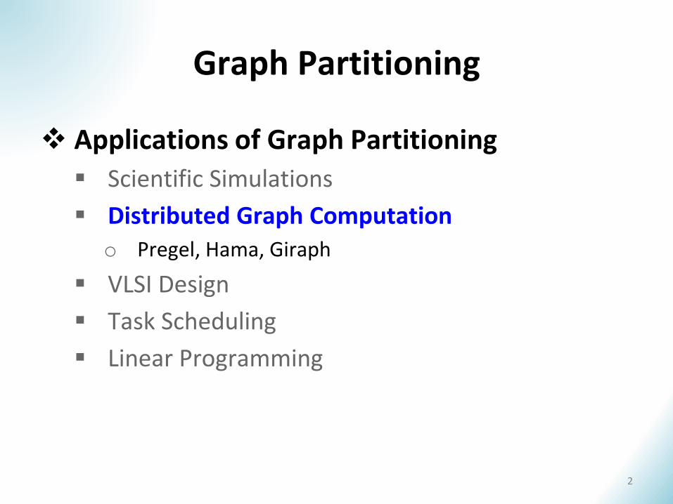
Applications of Graph Partitioning
Scientific Simulations
Distributed Graph Computationo Pregel, Hama, Giraph
VLSI Design
Task Scheduling
Linear Programming
2
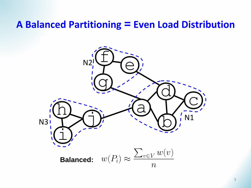
A Balanced Partitioning = Even Load Distribution
N3N1
N2
Balanced:
3
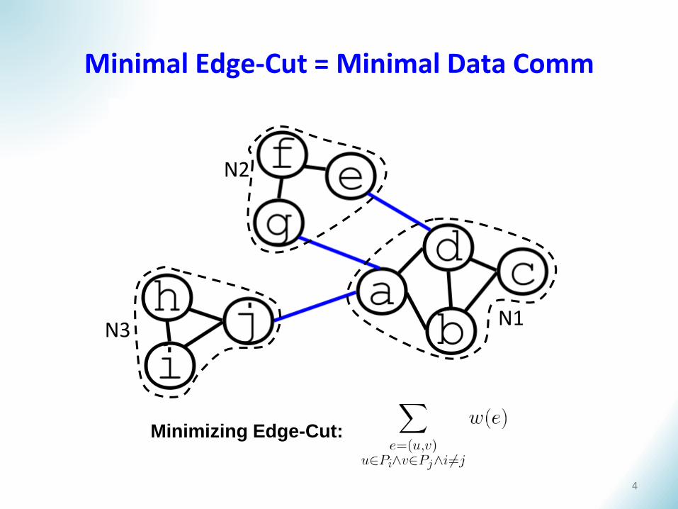
Minimal Edge-Cut = Minimal Data Comm
N3N1
N2
Minimizing Edge-Cut:
4
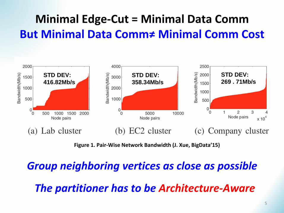
Minimal Edge-Cut = Minimal Data Comm But Minimal Data Comm≠ Minimal Comm Cost
Group neighboring vertices as close as possible
5
The partitioner has to be Architecture-Aware
Figure 1. Pair-Wise Network Bandwidth (J. Xue, BigData’15)
STD DEV:
416.82Mb/s
STD DEV:
358.34Mb/s
STD DEV:
269 . 71Mb/s
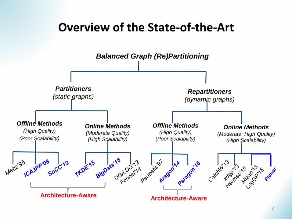
Overview of the State-of-the-Art
Balanced Graph (Re)Partitioning
Partitioners
(static graphs)Repartitioners
(dynamic graphs)
Offline Methods
(High Quality)
(Poor Scalability)
Online Methods(Moderate Quality)
(High Scalability)
Offline Methods(High Quality)
(Poor Scalability)
Online Methods(Moderate~High Quality)
(High Scalability)
Architecture-AwareArchitecture-Aware
6
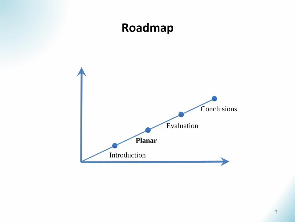
Roadmap
7
Introduction
Planar
Evaluation
Conclusions
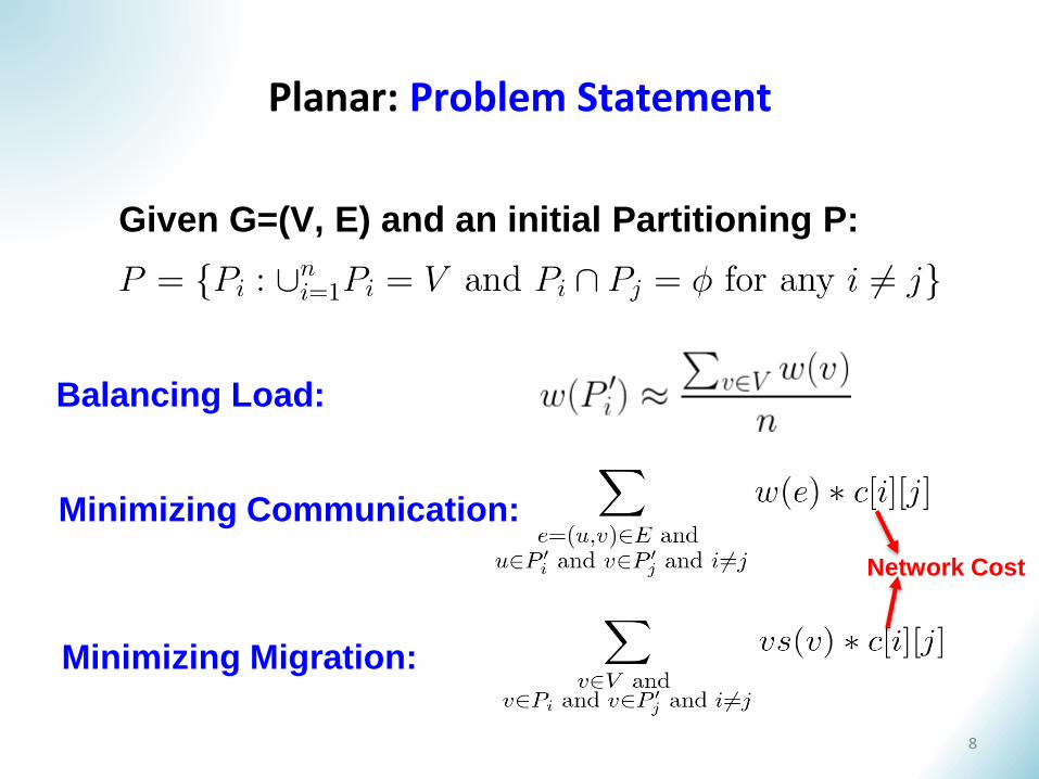
Planar: Problem Statement
Given G=(V, E) and an initial Partitioning P:
Minimizing Communication:
Balancing Load:
8
Network Cost
Minimizing Migration:
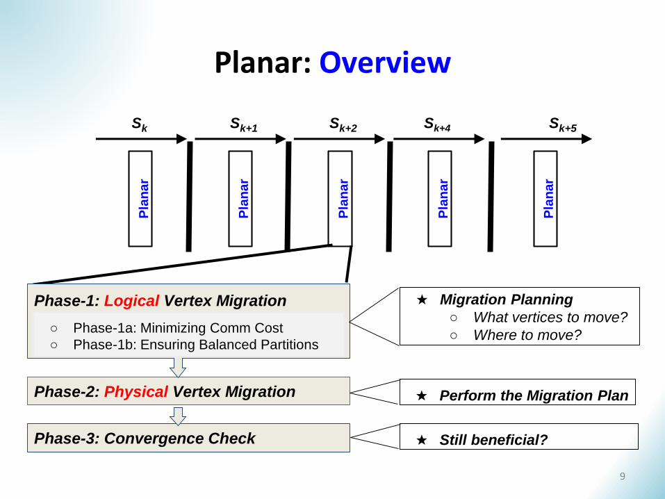
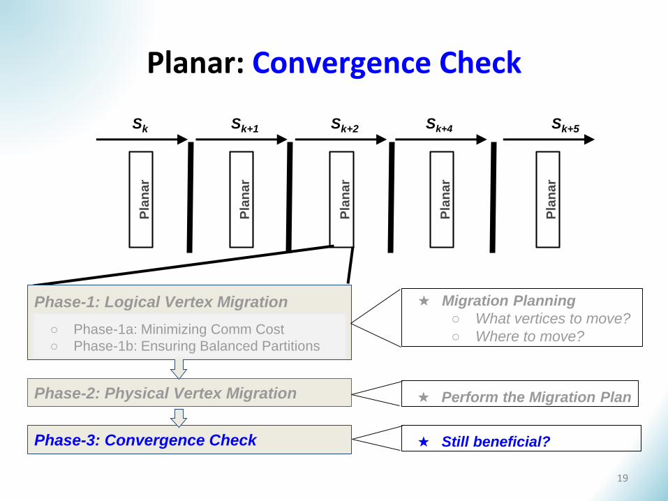
Planar: Overview
Phase-1: Logical Vertex Migration
Phase-2: Physical Vertex Migration
Phase-3: Convergence Check
★ Migration Planning
○ What vertices to move?
○ Where to move?
★ Still beneficial?
★ Perform the Migration Plan
Sk Sk+1 Sk+2 Sk+4 Sk+5
Pla
na
r
Pla
na
r
Pla
na
r
Pla
na
r
Pla
na
r
○ Phase-1a: Minimizing Comm Cost
○ Phase-1b: Ensuring Balanced Partitions
9
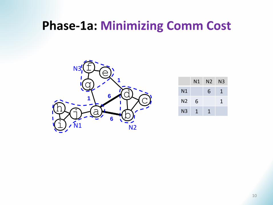
Phase-1a: Minimizing Comm Cost
N1 N2 N3
N1 6 1
N2 6 1
N3 1 1
N1 N2
N3
6
6
1
1
10
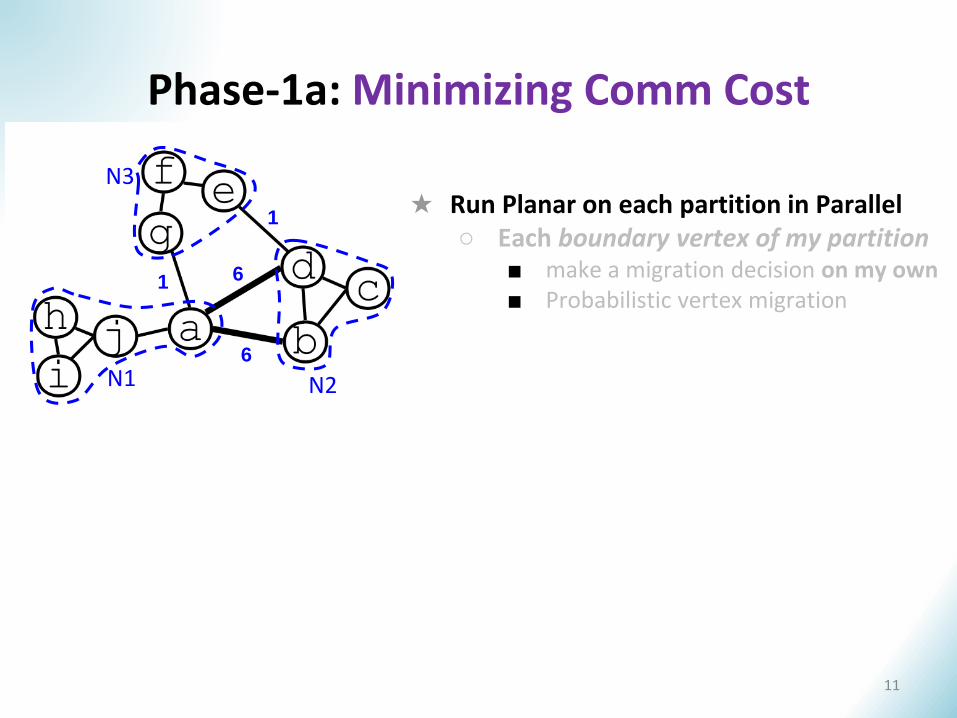
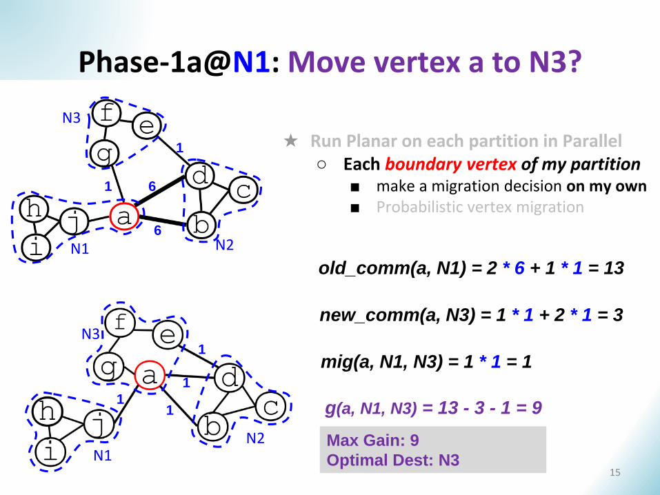
★ Run Planar on each partition in Parallel○ Each boundary vertex of my partition
■ make a migration decision on my own■ Probabilistic vertex migration
N1 N2
N3
6
6
1
1
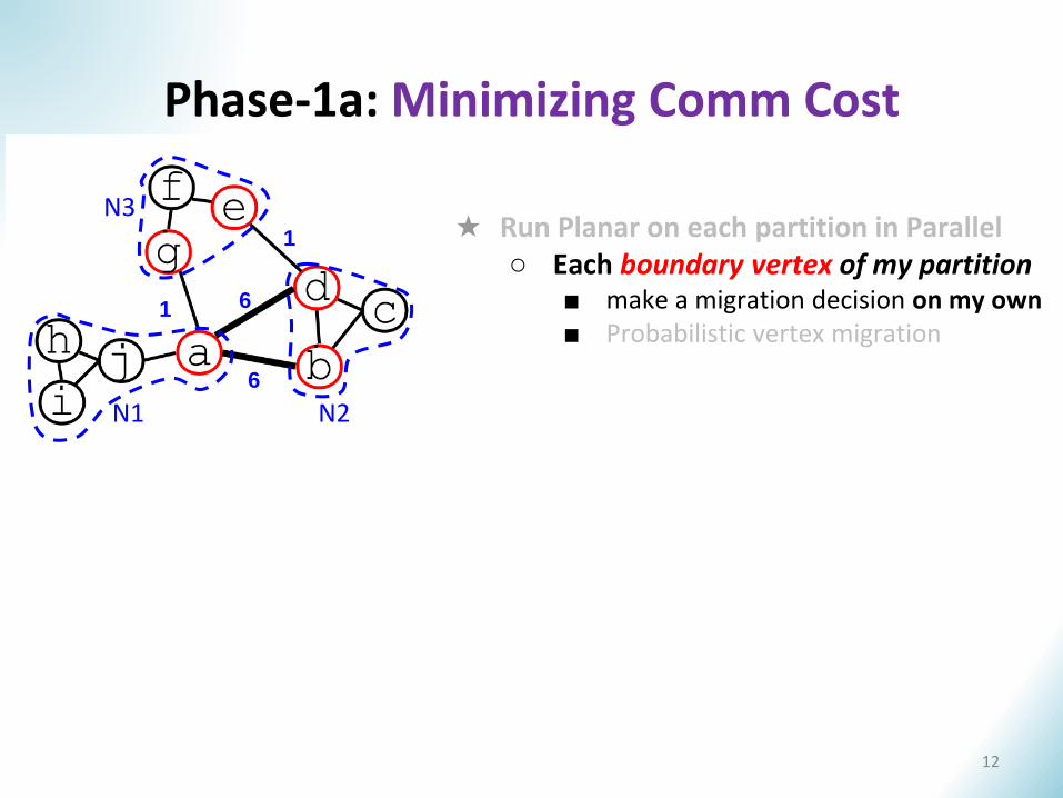
Phase-1a: Minimizing Comm Cost
11
N1 N2
N3
Phase-1a: Minimizing Comm Cost
6
6
1
1
12
★ Run Planar on each partition in Parallel○ Each boundary vertex of my partition
■ make a migration decision on my own■ Probabilistic vertex migration
N1 N2
N3
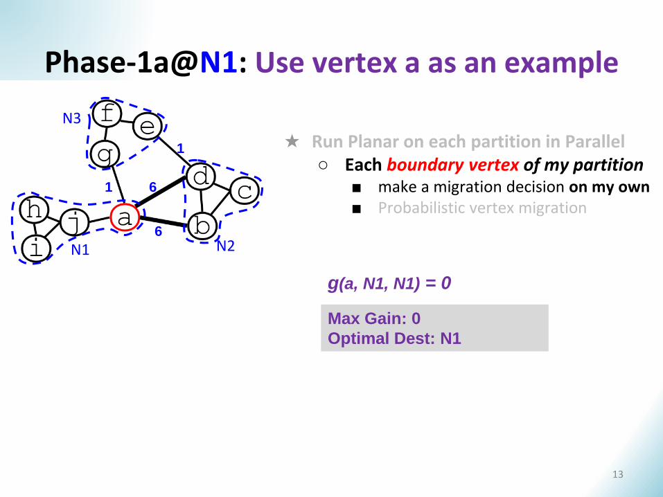
Phase-1a@N1: Use vertex a as an example
6
6
1
1
13
g(a, N1, N1) = 0
★ Run Planar on each partition in Parallel○ Each boundary vertex of my partition
■ make a migration decision on my own■ Probabilistic vertex migration
Max Gain: 0
Optimal Dest: N1
N1 N2
N3
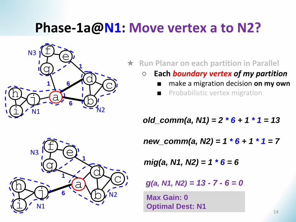
Phase-1a@N1: Move vertex a to N2?
new_comm(a, N2) = 1 * 6 + 1 * 1 = 7
g(a, N1, N2) = 13 - 7 - 6 = 0
old_comm(a, N1) = 2 * 6 + 1 * 1 = 13
mig(a, N1, N2) = 1 * 6 = 6
14
★ Run Planar on each partition in Parallel○ Each boundary vertex of my partition
■ make a migration decision on my own■ Probabilistic vertex migration
Max Gain: 0
Optimal Dest: N1
6
6
1
1
N1
N2
N3
6
1
1
N2
N3
6
6
1
N1
Phase-1a@N1: Move vertex a to N3?
15
new_comm(a, N3) = 1 * 1 + 2 * 1 = 3
old_comm(a, N1) = 2 * 6 + 1 * 1 = 13
mig(a, N1, N3) = 1 * 1 = 1
g(a, N1, N3) = 13 - 3 - 1 = 9
★ Run Planar on each partition in Parallel○ Each boundary vertex of my partition
■ make a migration decision on my own■ Probabilistic vertex migration
Max Gain: 9
Optimal Dest: N3
1
N1N2
N3
11
1
1
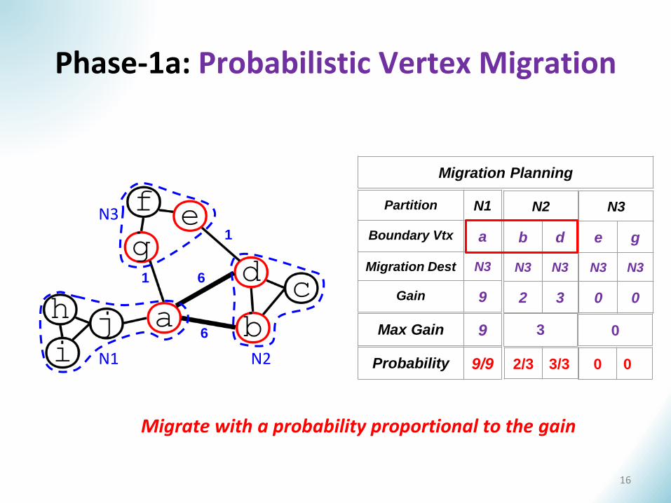
Phase-1a: Probabilistic Vertex Migration
Partition N1
Boundary Vtx a
Migration Dest N3
Gain 9
N2
b d
N3 N3
2 3
Migration Planning
Probability 9/9 2/3 3/3
Max Gain 9 3
16
N1 N2
N3
6
6
1
1
Migrate with a probability proportional to the gain
0
0 0
N3
e g
N3 N3
0 0
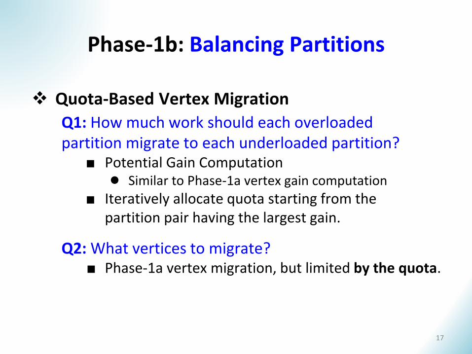
Phase-1b: Balancing Partitions
Quota-Based Vertex Migration
Q2: What vertices to migrate?■ Phase-1a vertex migration, but limited by the quota.
Q1: How much work should each overloaded partition migrate to each underloaded partition?
■ Potential Gain Computation● Similar to Phase-1a vertex gain computation
■ Iteratively allocate quota starting from the partition pair having the largest gain.
17
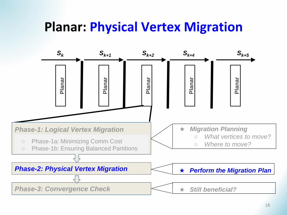
Planar: Physical Vertex Migration
Phase-1: Logical Vertex Migration
Phase-2: Physical Vertex Migration
Phase-3: Convergence Check
★ Migration Planning
○ What vertices to move?
○ Where to move?
★ Still beneficial?
★ Perform the Migration Plan
Sk Sk+1 Sk+2 Sk+4 Sk+5
Pla
na
r
Pla
na
r
Pla
na
r
Pla
na
r
Pla
na
r
○ Phase-1a: Minimizing Comm Cost
○ Phase-1b: Ensuring Balanced Partitions
18
Planar: Convergence Check
Phase-1: Logical Vertex Migration
Phase-2: Physical Vertex Migration
Phase-3: Convergence Check
★ Migration Planning
○ What vertices to move?
○ Where to move?
★ Still beneficial?
★ Perform the Migration Plan
Sk Sk+1 Sk+2 Sk+4 Sk+5
Pla
na
r
Pla
na
r
Pla
na
r
Pla
na
r
Pla
na
r
○ Phase-1a: Minimizing Comm Cost
○ Phase-1b: Ensuring Balanced Partitions
19
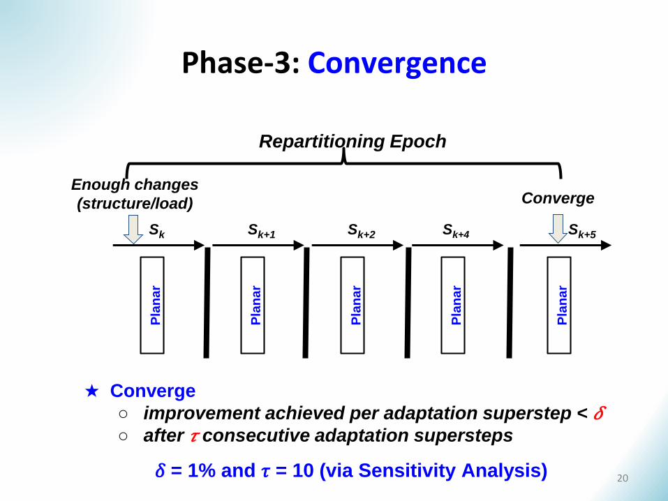
Phase-3: Convergence
Sk Sk+1 Sk+2 Sk+4 Sk+5
ConvergeEnough changes
(structure/load)
Repartitioning Epoch
★ Converge
○ improvement achieved per adaptation superstep < 𝛿○ after 𝜏 consecutive adaptation supersteps
Pla
na
r
Pla
na
r
Pla
na
r
Pla
na
r
Pla
na
r
𝛿 = 1% and 𝜏 = 10 (via Sensitivity Analysis) 20
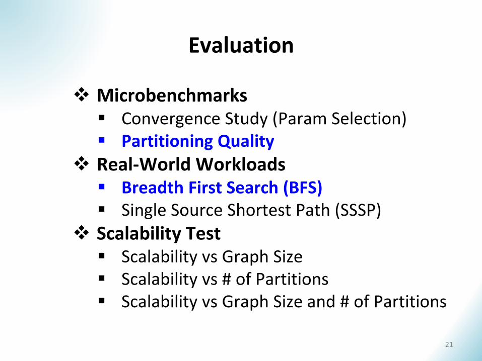
Evaluation
21
Microbenchmarks Convergence Study (Param Selection) Partitioning Quality
Real-World Workloads Breadth First Search (BFS) Single Source Shortest Path (SSSP)
Scalability Test Scalability vs Graph Size Scalability vs # of Partitions Scalability vs Graph Size and # of Partitions
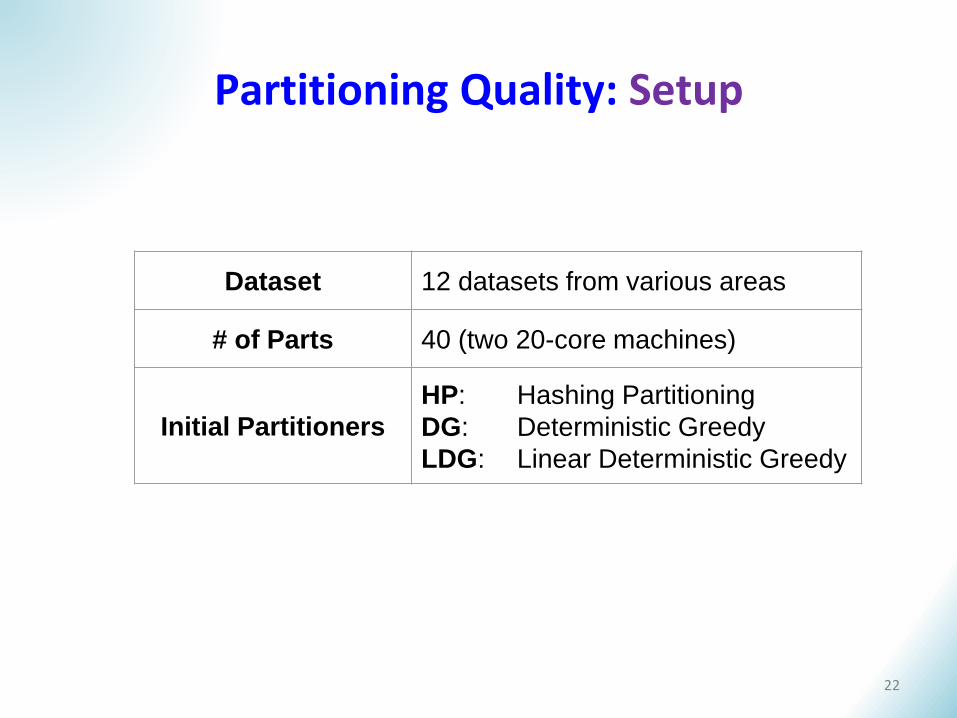
Partitioning Quality: Setup
Dataset 12 datasets from various areas
# of Parts 40 (two 20-core machines)
Initial Partitioners
HP: Hashing Partitioning
DG: Deterministic Greedy
LDG: Linear Deterministic Greedy
22
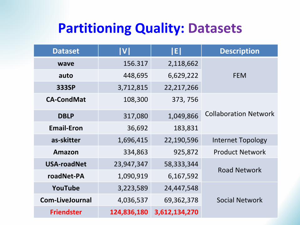
Partitioning Quality: Datasets
Dataset |V| |E| Description
wave 156.317 2,118,662
FEMauto 448,695 6,629,222
333SP 3,712,815 22,217,266
CA-CondMat 108,300 373, 756
Collaboration NetworkDBLP 317,080 1,049,866
Email-Eron 36,692 183,831
as-skitter 1,696,415 22,190,596 Internet Topology
Amazon 334,863 925,872 Product Network
USA-roadNet 23,947,347 58,333,344Road Network
roadNet-PA 1,090,919 6,167,592
YouTube 3,223,589 24,447,548
Social NetworkCom-LiveJournal 4,036,537 69,362,378
Friendster 124,836,180 3,612,134,270
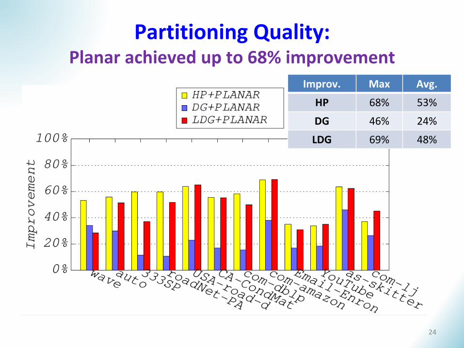
Partitioning Quality: Planar achieved up to 68% improvement
Improv. Max Avg.
HP 68% 53%
DG 46% 24%
LDG 69% 48%
24
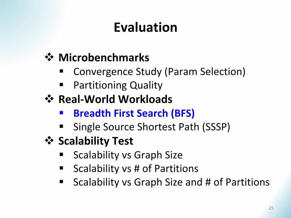
Evaluation
25
Microbenchmarks Convergence Study (Param Selection) Partitioning Quality
Real-World Workloads Breadth First Search (BFS) Single Source Shortest Path (SSSP)
Scalability Test Scalability vs Graph Size Scalability vs # of Partitions Scalability vs Graph Size and # of Partitions
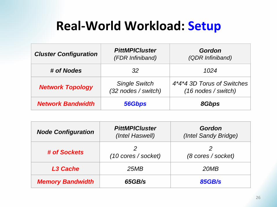
Real-World Workload: Setup
Cluster ConfigurationPittMPICluster
(FDR Infiniband)Gordon
(QDR Infiniband)
# of Nodes 32 1024
Network TopologySingle Switch
(32 nodes / switch)
4*4*4 3D Torus of Switches
(16 nodes / switch)
Network Bandwidth 56Gbps 8Gbps
Node ConfigurationPittMPICluster
(Intel Haswell)
Gordon
(Intel Sandy Bridge)
# of Sockets2
(10 cores / socket)
2
(8 cores / socket)
L3 Cache 25MB 20MB
Memory Bandwidth 65GB/s 85GB/s
26
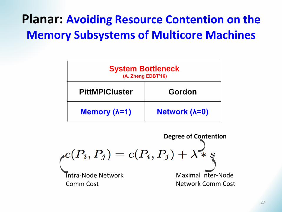
Planar: Avoiding Resource Contention on the Memory Subsystems of Multicore Machines
Intra-Node Network Comm Cost
Maximal Inter-Node Network Comm Cost
Degree of Contention
System Bottleneck(A. Zheng EDBT’16)
PittMPICluster Gordon
Memory (λ=1) Network (λ=0)
27
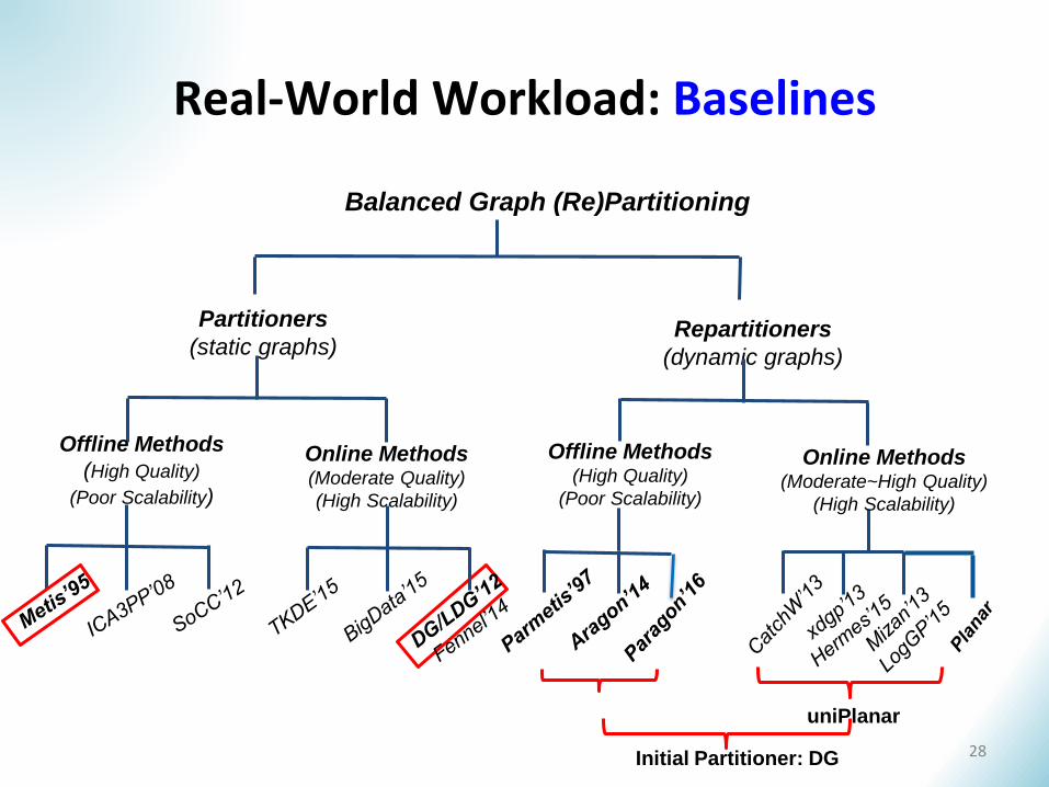
Real-World Workload: Baselines
Balanced Graph (Re)Partitioning
Partitioners
(static graphs)Repartitioners
(dynamic graphs)
Offline Methods
(High Quality)
(Poor Scalability)
Online Methods(Moderate Quality)
(High Scalability)
Offline Methods(High Quality)
(Poor Scalability)
Online Methods(Moderate~High Quality)
(High Scalability)
uniPlanar
Initial Partitioner: DG 28
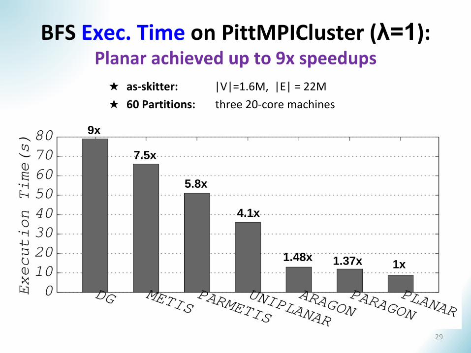
BFS Exec. Time on PittMPICluster (λ=1): Planar achieved up to 9x speedups
9x
7.5x
5.8x
4.1x
1.48x 1.37x 1x
29
★ as-skitter: |V|=1.6M, |E| = 22M
★ 60 Partitions: three 20-core machines
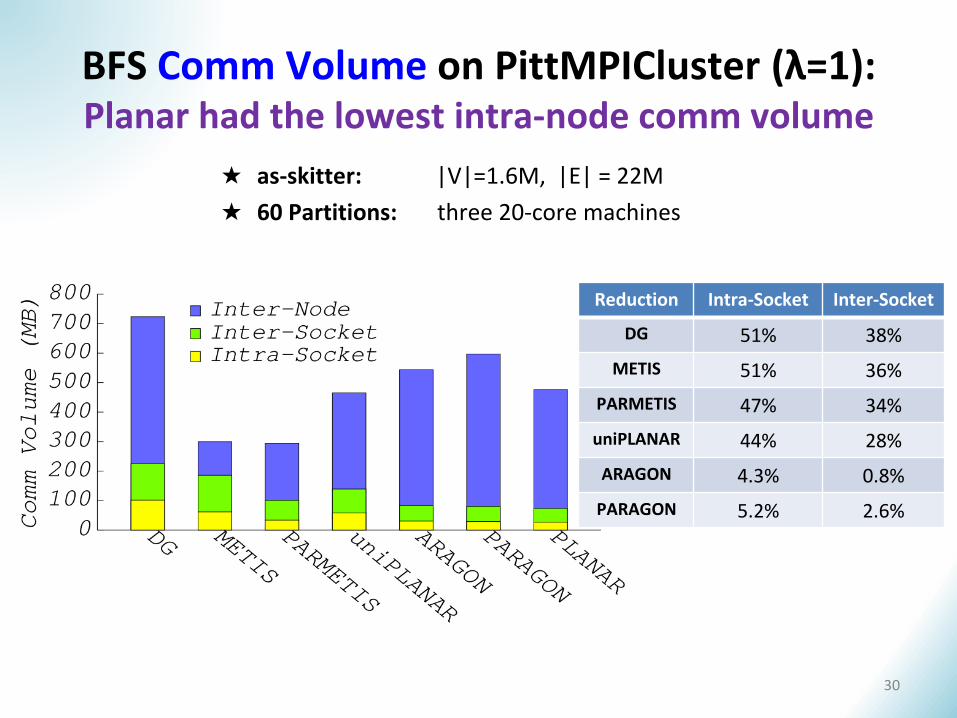
BFS Comm Volume on PittMPICluster (λ=1): Planar had the lowest intra-node comm volume
★ as-skitter: |V|=1.6M, |E| = 22M
★ 60 Partitions: three 20-core machines
Reduction Intra-Socket Inter-Socket
DG 51% 38%
METIS 51% 36%
PARMETIS 47% 34%
uniPLANAR 44% 28%
ARAGON 4.3% 0.8%
PARAGON 5.2% 2.6%
30
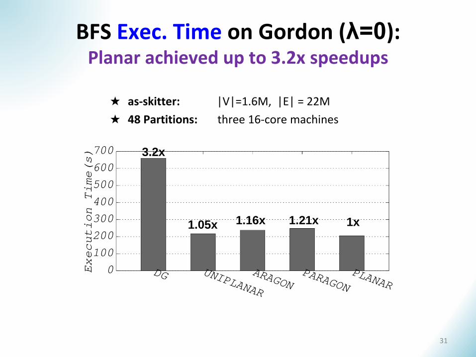
3.2x
1.05x 1.16x 1.21x
BFS Exec. Time on Gordon (λ=0):Planar achieved up to 3.2x speedups
1x
31
★ as-skitter: |V|=1.6M, |E| = 22M
★ 48 Partitions: three 16-core machines
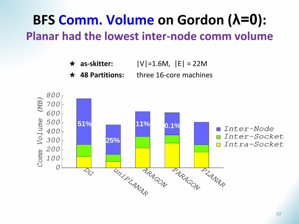
51%
25%
11% 0.1%
BFS Comm. Volume on Gordon (λ=0): Planar had the lowest inter-node comm volume
32
★ as-skitter: |V|=1.6M, |E| = 22M
★ 48 Partitions: three 16-core machines
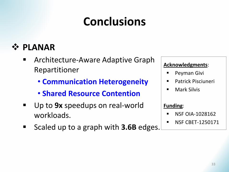
Conclusions
PLANAR
Architecture-Aware Adaptive Graph Repartitioner
• Communication Heterogeneity
• Shared Resource Contention
Up to 9x speedups on real-world workloads.
Scaled up to a graph with 3.6B edges.
Acknowledgments:
Peyman Givi
Patrick Pisciuneri
Mark Silvis
Funding:
NSF OIA-1028162
NSF CBET-1250171
33
Thank You!
Email: [email protected]: http://people.cs.pitt.edu/~anz28/ADMT: http://db.cs.pitt.edu/group/
34
Backup Slides
35
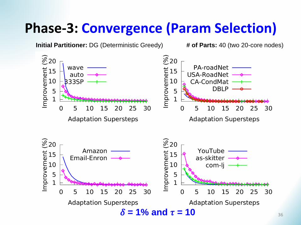
Phase-3: Convergence (Param Selection)
𝛿 = 1% and 𝜏 = 10
Initial Partitioner: DG (Deterministic Greedy) # of Parts: 40 (two 20-core nodes)
36
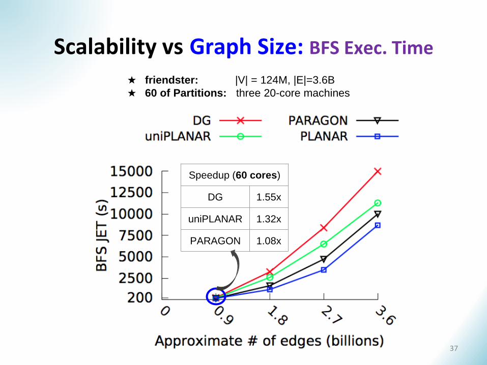
Scalability vs Graph Size: BFS Exec. Time
★ friendster: |V| = 124M, |E|=3.6B
★ 60 of Partitions: three 20-core machines
Speedup (60 cores)
DG 1.55x
uniPLANAR 1.32x
PARAGON 1.08x
37
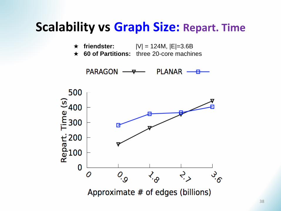
Scalability vs Graph Size: Repart. Time
38
★ friendster: |V| = 124M, |E|=3.6B
★ 60 of Partitions: three 20-core machines
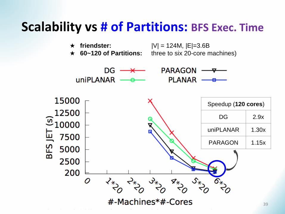
Scalability vs # of Partitions: BFS Exec. Time
Speedup (120 cores)
DG 2.9x
uniPLANAR 1.30x
PARAGON 1.15x
★ friendster: |V| = 124M, |E|=3.6B
★ 60~120 of Partitions: three to six 20-core machines)
39
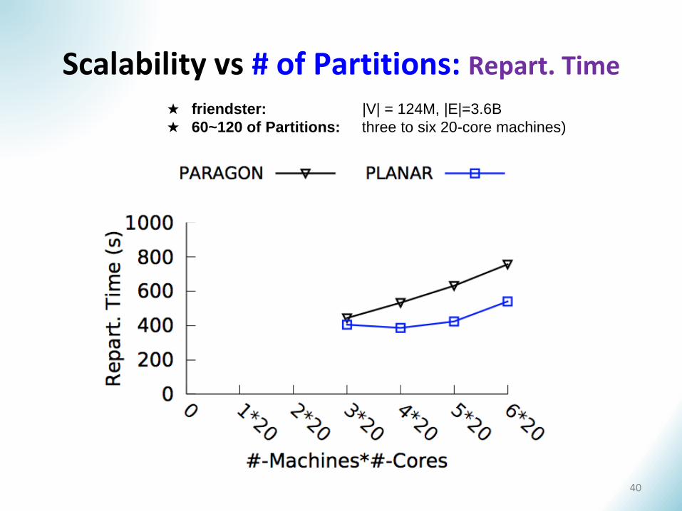
Scalability vs # of Partitions: Repart. Time
40
★ friendster: |V| = 124M, |E|=3.6B
★ 60~120 of Partitions: three to six 20-core machines)
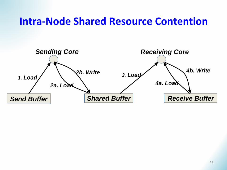
Intra-Node Shared Resource Contention
Send Buffer
Sending Core Receiving Core
Receive BufferShared Buffer
1. Load3. Load2b. Write
2a. Load 4a. Load
4b. Write
41
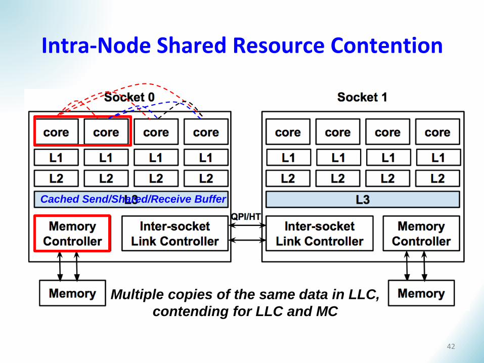
Cached Send/Shared/Receive Buffer
Intra-Node Shared Resource Contention
Multiple copies of the same data in LLC,
contending for LLC and MC
42
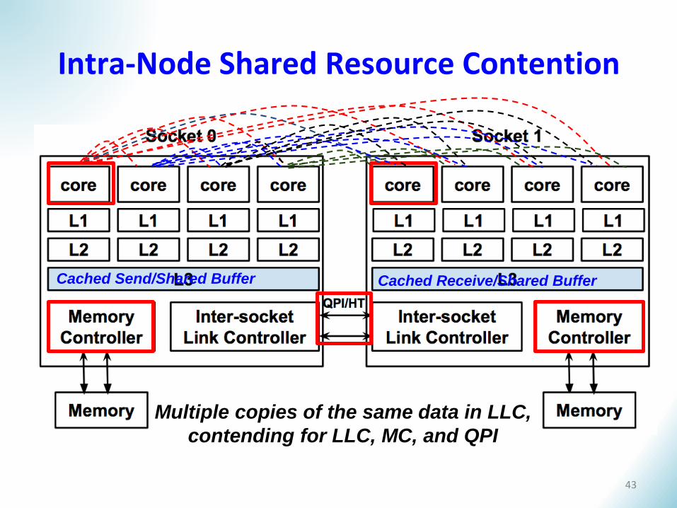
Intra-Node Shared Resource Contention
Cached Send/Shared Buffer Cached Receive/Shared Buffer
Multiple copies of the same data in LLC,
contending for LLC, MC, and QPI
43
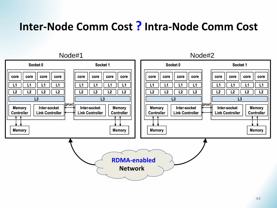
Inter-Node Comm Cost ? Intra-Node Comm Cost
Network
Node#1 Node#2
RDMA-enabled
44
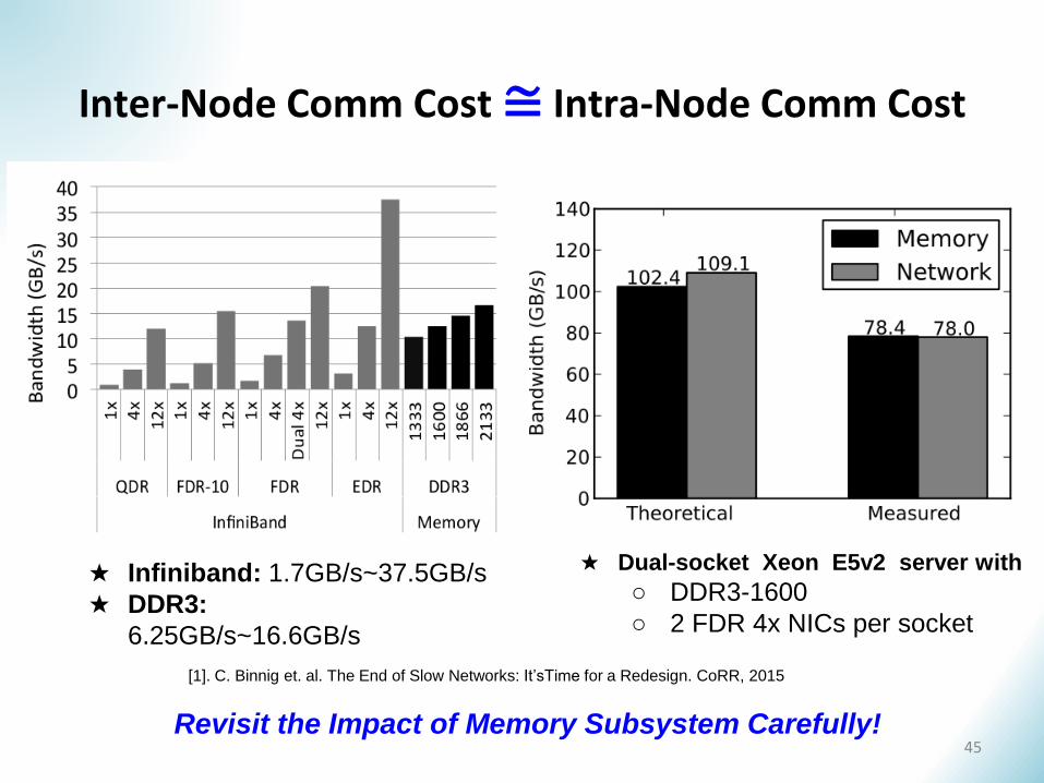
Inter-Node Comm Cost≅ Intra-Node Comm Cost
[1]. C. Binnig et. al. The End of Slow Networks: It’sTime for a Redesign. CoRR, 2015
★ Dual-socket Xeon E5v2 server with
○ DDR3-1600
○ 2 FDR 4x NICs per socket
Revisit the Impact of Memory Subsystem Carefully!
★ Infiniband: 1.7GB/s~37.5GB/s
★ DDR3:
6.25GB/s~16.6GB/s
45
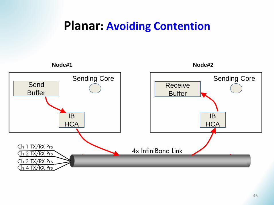
Planar: Avoiding Contention
Send
Buffer
Sending Core
Node#1
IB
HCA
Receive
Buffer
Sending Core
Node#2
IB
HCA
46

![Fabrication-aware Design with Intersecting Planar …...Y. Schwartzburg & M. Pauly / Fabrication-aware Design with Intersecting Planar Pieces Pop-up designs [Gla02,LSH10,LJGH11] aim](https://img.pdfslide.net/doc/110x75/5e46c57efdbb2f676a7c14c3/fabrication-aware-design-with-intersecting-planar-y-schwartzburg-m-pauly.jpg)
![Beyond Layers: A 3D-Aware Toolpath Algorithm for Fused …mettu/publications/Mettu_ICRA_2016... · 2016. 1. 30. · Slic3r [17] path generator, which follows the iso-planar method](https://img.pdfslide.net/doc/110x75/5fd84b744e571a267e2781bf/beyond-layers-a-3d-aware-toolpath-algorithm-for-fused-mettupublicationsmettuicra2016.jpg)
![Lightweight and Energy-Aware Wireless Mesh Routing for ...staff.ui.ac.id/system/files/users/riri/publication/paper_lukman_inteli... · Optimized Link State Routing (OLSR) [9], and](https://img.pdfslide.net/doc/110x75/5f5c9ae7b5e64a779b3eea85/lightweight-and-energy-aware-wireless-mesh-routing-for-staffuiacidsystemfilesusersriripublicationpaperlukmaninteli.jpg)