Embed Size (px)
Citation preview

Astronomy & Astrophysics manuscript no. Planck˙Constraints˙on˙primordial˙non-Gaussianity c© ESO 2013December 5, 2013
Planck 2013 results. XXIV. Constraints on primordialnon-Gaussianity
Planck Collaboration: P. A. R. Ade87, N. Aghanim60, C. Armitage-Caplan93, M. Arnaud73, M. Ashdown70,6, F. Atrio-Barandela18, J. Aumont60,C. Baccigalupi86, A. J. Banday96,9, R. B. Barreiro67, J. G. Bartlett1,68, N. Bartolo34∗, E. Battaner97, K. Benabed61,95, A. Benoıt58,
A. Benoit-Levy25,61,95, J.-P. Bernard96,9, M. Bersanelli37,51, P. Bielewicz96,9,86, J. Bobin73, J. J. Bock68,10, A. Bonaldi69, L. Bonavera67, J. R. Bond8,J. Borrill13,90, F. R. Bouchet61,95, M. Bridges70,6,64, M. Bucher1, C. Burigana50,35, R. C. Butler50, J.-F. Cardoso74,1,61, A. Catalano75,72,
A. Challinor64,70,11, A. Chamballu73,15,60, H. C. Chiang29,7, L.-Y Chiang63, P. R. Christensen82,41, S. Church92, D. L. Clements56, S. Colombi61,95,L. P. L. Colombo24,68, F. Couchot71, A. Coulais72, B. P. Crill68,83, A. Curto6,67, F. Cuttaia50, L. Danese86, R. D. Davies69, R. J. Davis69, P. de
Bernardis36, A. de Rosa50, G. de Zotti46,86, J. Delabrouille1, J.-M. Delouis61,95, F.-X. Desert54, J. M. Diego67, H. Dole60,59, S. Donzelli51,O. Dore68,10, M. Douspis60, A. Ducout61, J. Dunkley93, X. Dupac43, G. Efstathiou64, F. Elsner61,95, T. A. Enßlin78, H. K. Eriksen65, J. Fergusson11,
F. Finelli50,52, O. Forni96,9, M. Frailis48, E. Franceschi50, S. Galeotta48, K. Ganga1, M. Giard96,9, Y. Giraud-Heraud1, J. Gonzalez-Nuevo67,86,K. M. Gorski68,98, S. Gratton70,64, A. Gregorio38,48, A. Gruppuso50, F. K. Hansen65, D. Hanson79,68,8, D. Harrison64,70, A. Heavens56,S. Henrot-Versille71, C. Hernandez-Monteagudo12,78, D. Herranz67, S. R. Hildebrandt10, E. Hivon61,95, M. Hobson6, W. A. Holmes68,
A. Hornstrup16, W. Hovest78, K. M. Huffenberger27, A. H. Jaffe56, T. R. Jaffe96,9, W. C. Jones29, M. Juvela28, E. Keihanen28, R. Keskitalo22,13,T. S. Kisner77, J. Knoche78, L. Knox31, M. Kunz17,60,3, H. Kurki-Suonio28,45, F. Lacasa60, G. Lagache60, A. Lahteenmaki2,45, J.-M. Lamarre72,A. Lasenby6,70, R. J. Laureijs44, C. R. Lawrence68, J. P. Leahy69, R. Leonardi43, J. Lesgourgues94,85, A. Lewis26, M. Liguori34, P. B. Lilje65,
M. Linden-Vørnle16, M. Lopez-Caniego67, P. M. Lubin32, J. F. Macıas-Perez75, B. Maffei69, D. Maino37,51, N. Mandolesi50,5,35, A. Mangilli61,D. Marinucci40, M. Maris48, D. J. Marshall73, P. G. Martin8, E. Martınez-Gonzalez67, S. Masi36, M. Massardi49, S. Matarrese34, F. Matthai78,
P. Mazzotta39, P. R. Meinhold32, A. Melchiorri36,53, L. Mendes43, A. Mennella37,51, M. Migliaccio64,70, S. Mitra55,68, M.-A. Miville-Deschenes60,8,A. Moneti61, L. Montier96,9, G. Morgante50, D. Mortlock56, A. Moss88, D. Munshi87, J. A. Murphy81, P. Naselsky82,41, P. Natoli35,4,50,C. B. Netterfield20, H. U. Nørgaard-Nielsen16, F. Noviello69, D. Novikov56, I. Novikov82, S. Osborne92, C. A. Oxborrow16, F. Paci86,
L. Pagano36,53, F. Pajot60, D. Paoletti50,52, F. Pasian48, G. Patanchon1, H. V. Peiris25, O. Perdereau71, L. Perotto75, F. Perrotta86, F. Piacentini36,M. Piat1, E. Pierpaoli24, D. Pietrobon68, S. Plaszczynski71, E. Pointecouteau96,9, G. Polenta4,47, N. Ponthieu60,54, L. Popa62, T. Poutanen45,28,2,
G. W. Pratt73, G. Prezeau10,68, S. Prunet61,95, J.-L. Puget60, J. P. Rachen21,78, B. Racine1, R. Rebolo66,14,42, M. Reinecke78, M. Remazeilles69,60,1,C. Renault75, A. Renzi86, S. Ricciardi50, T. Riller78, I. Ristorcelli96,9, G. Rocha68,10, C. Rosset1, G. Roudier1,72,68, J. A. Rubino-Martın66,42,
B. Rusholme57, M. Sandri50, D. Santos75, G. Savini84, D. Scott23, M. D. Seiffert68,10, E. P. S. Shellard11, K. Smith29, L. D. Spencer87,J.-L. Starck73, V. Stolyarov6,70,91, R. Stompor1, R. Sudiwala87, R. Sunyaev78,89, F. Sureau73, P. Sutter61, D. Sutton64,70, A.-S. Suur-Uski28,45,J.-F. Sygnet61, J. A. Tauber44, D. Tavagnacco48,38, L. Terenzi50, L. Toffolatti19,67, M. Tomasi51, M. Tristram71, M. Tucci17,71, J. Tuovinen80,
L. Valenziano50, J. Valiviita45,28,65, B. Van Tent76, J. Varis80, P. Vielva67, F. Villa50, N. Vittorio39, L. A. Wade68, B. D. Wandelt61,95,33, M. White30,S. D. M. White78, D. Yvon15, A. Zacchei48, and A. Zonca32
(Affiliations can be found after the references)
Received xxxx, Accepted xxxxx
ABSTRACT
The Planck nominal mission cosmic microwave background (CMB) maps yield unprecedented constraints on primordial non-Gaussianity (NG).Using three optimal bispectrum estimators, separable template-fitting (KSW), binned, and modal, we obtain consistent values for the primordiallocal, equilateral, and orthogonal bispectrum amplitudes, quoting as our final result f local
NL = 2.7 ± 5.8, f equilNL = −42 ± 75, and f ortho
NL = −25 ± 39(68% CL statistical). Non-Gaussianity is detected in the data; using skew-C` statistics we find a nonzero bispectrum from residual point sources,and the Integrated-Sachs-Wolfe-lensing bispectrum at a level expected in the ΛCDM scenario. The results are based on comprehensive cross-validation of these estimators on Gaussian and non-Gaussian simulations, are stable across component separation techniques, pass an extensivesuite of tests, and are confirmed by skew-C`, wavelet bispectrum and Minkowski functional estimators. Beyond estimates of individual shapeamplitudes, we present model-independent, three-dimensional reconstructions of the Planck CMB bispectrum and thus derive constraints onearly-Universe scenarios that generate primordial NG, including general single-field models of inflation, excited initial states (non-Bunch-Daviesvacua), and directionally-dependent vector models. We provide an initial survey of scale-dependent feature and resonance models. These resultsbound both general single-field and multi-field model parameter ranges, such as the speed of sound, cs ≥ 0.02 (95% CL), in an effective fieldtheory parametrization, and the curvaton decay fraction rD ≥ 0.15 (95% CL). The Planck data significantly limit the viable parameter space of theekpyrotic/cyclic scenarios. The amplitude of the four-point function in the local model τNL < 2800 (95% CL). Taken together, these constraintsrepresent the highest precision tests to date of physical mechanisms for the origin of cosmic structure.
Key words. cosmology: cosmic background radiation – cosmology: observations – cosmology: theory – cosmology: early Universe – cosmology:inflation – methods: data analysis
∗ Corresponding author: Nicola Bartolo [email protected]
1
arX
iv:1
303.
5084
v2 [
astr
o-ph
.CO
] 3
Dec
201
3

Planck Collaboration: Planck 2013 Results. XXIV. Constraints on primordial NG
1. Introduction
This paper, one of a set associated with the 2013 release ofdata from the Planck1 mission (Planck Collaboration I 2013),describes the constraints on primordial non-Gaussianity (NG)obtained using the cosmic microwave background (CMB) mapsderived from the data acquired by Planck during its nominal op-erations period, i.e., between 12 August 2009 and 27 November2010.
Primordial NG is one of the most informative finger-prints of the origin of structure in the Universe, prob-ing physics at extremely high energy scales inaccessi-ble to laboratory experiments. Possible departures froma purely Gaussian distribution of the CMB anisotropiesprovide powerful observational access to this extremephysics (Allen et al. 1987; Salopek & Bond 1990; Falk et al.1993; Gangui et al. 1994; Verde et al. 2000; Gangui & Martin2000b; Wang & Kamionkowski 2000; Komatsu & Spergel2001; Acquaviva et al. 2003; Maldacena 2003; Babich et al.2004; for recent reviews Bartolo et al. 2004a, Liguori et al.2010, Chen 2010b, Komatsu 2010, Yadav & Wandelt 2010).A robust detection of primordial NG – or a strong constrainton it – discriminates among competing mechanisms for thegeneration of the cosmological perturbations in the earlyUniverse. Different inflationary models, firmly rooted in moderntheoretical particle physics, predict different amplitudes, shapes,and scale dependence of NG. As a result, primordial NG iscomplementary to the scalar-spectral index of curvature pertur-bations and the tensor-to-scalar amplitude ratio, distinguishingbetween inflationary models that are degenerate on the basisof their power spectra alone. Even in the simplest models ofinflation, consisting of a single slowly-rolling scalar field, asmall (but calculable) level of NG is predicted (Acquaviva et al.2003; Maldacena 2003); this is undetectable in present-qualityCMB and large-scale structure measurements. However, asdemonstrated by a large body of work in recent years, extendingthis simplest paradigm will generically lead to detectable levelsof NG in CMB anisotropies. Critically, a robust detectionof primordial NG would rule out all canonical single-fieldslow-roll models of inflation, pointing to physics beyond thesimplest “textbook” picture of inflation. Conversely, significantimprovements in the constraints on primordial NG stronglylimit extensions to the simplest paradigm, thus providingpowerful clues to the physical mechanism that generated cosmicstructure.
If the primordial fluctuations are Gaussian-distributed, thenthey are completely characterised by their two-point correlationfunction, or equivalently, their power spectrum. If they are non-Gaussian, there is additional statistical information in the higher-order correlation functions, which is not captured by the two-point correlation function. In particular, the 3-point correlationfunction, or its Fourier counterpart, the bispectrum, is impor-tant because it is the lowest-order statistic that can distinguishbetween Gaussian and non-Gaussian perturbations. One of themain goals of this paper is to constrain the amplitude and shapeof primordial NG using the angular bispectrum of the CMBanisotropies. The CMB angular bispectrum is related to the pri-
1 Planck (http://www.esa.int/Planck) is a project of theEuropean Space Agency (ESA) with instruments provided by two sci-entific consortia funded by ESA member states (in particular the leadcountries France and Italy), with contributions from NASA (USA) andtelescope reflectors provided by a collaboration between ESA and a sci-entific consortium led and funded by Denmark.
mordial bispectrum defined by
〈Φ(k1)Φ(k2)Φ(k3)〉 = (2π)3δ(3)(k1 + k2 + k3)BΦ(k1, k2, k3). (1)
Here we define the potential Φ in terms of the comoving cur-vature perturbation ζ on super-horizon scales by Φ ≡ (3/5)ζ.In matter domination, on super-horizon scales, Φ is equivalentto Bardeen’s gauge-invariant gravitational potential (Bardeen1980), and we adopt this notation for historical consistency.The bispectrum BΦ(k1, k2, k3) measures the correlation amongthree perturbation modes. Assuming translational and rotationalinvariance, it depends only on the magnitudes of the threewavevectors. In general the bispectrum can be written as
BΦ(k1, k2, k3) = fNLF(k1, k2, k3) . (2)
Here, fNL is the so-called “nonlinearity parameter”(Gangui et al. 1994; Wang & Kamionkowski 2000;Komatsu & Spergel 2001; Babich et al. 2004), a dimen-sionless parameter measuring the amplitude of NG. Thebispectrum is measured by sampling triangles in Fourier space.The dependence of the function F(k1, k2, k3) on the type oftriangle (i.e., the configuration) formed by the three wavevec-tors describes the shape of the bispectrum (Babich et al.2004), which encodes much physical information. It canalso encode the scale dependence, i.e., the running, of thebispectrum (Chen 2005c).2 Different NG shapes are linkedto distinctive physical mechanisms that can generate suchnon-Gaussian fingerprints in the early Universe. For example,the so-called “local” NG (Gangui et al. 1994; Verde et al.2000; Wang & Kamionkowski 2000; Komatsu & Spergel 2001)is characterized by a signal that is maximal for “squeezed”triangles with k1 � k2 ' k3 (or permutations; Maldacena2003) which occurs, in general, when the primordial NG isgenerated on super-horizon scales. Conversely, “equilateral”NG (Babich et al. 2004) peaks for equilateral configurationsk1 ≈ k2 ≈ k3, due to correlations between fluctuation modesthat are of comparable wavelengths, which can occur if thethree perturbation modes mostly interact when they cross thehorizon approximately at the same time. Other relevant shapesinclude the so-called “folded” (or flattened) NG (Chen et al.2007b), which is due to correlations between perturbationmodes that are enhanced for k1 + k2 ≈ k3, or the “orthogonal”NG (Senatore et al. 2010) that generates a signal with a positivepeak at the equilateral configuration and a negative peak at thefolded configuration.
We now sketch how non-Gaussian information in the ini-tial conditions is transferred to observable quantities (in thisinstance, the CMB anisotropies) in the context of inflation.Primordial perturbations in the inflaton field(s) φ(x, t) = φ0(t) +δφ(x, t) (where δφ denotes quantum fluctuations about thebackground value φ0(t)) can be characterized by the comov-ing curvature perturbation ζ, since this is conserved on super-horizon scales for adiabatic perturbations. The inflaton fluctu-ations δφ (in the flat gauge) induce a curvature perturbation3
2 Specifically, one can define the shape of the bispectrum as the de-pendence of F(k1, k2, k3)(k1k2k3)2 on the ratios of momenta, e.g., (k2/k1)and (k3/k1), once the overall scale of the triangle K = k1 + k2 + k3 isfixed. The scale dependence of the bispectrum can be characterized bythe dependence of F(k1, k2, k3)(k1k2k3)2 on the overall scale K, once theratios (k2/k1) and (k3/k1) are fixed (see, e.g., Chen 2010b).
3 For the curvature perturbation, we follow the notation and signconventions of Komatsu et al. (2011). ζ is also sometimes denotedR (see e.g., Lidsey et al. 1997, Lyth & Riotto 1999 and referencestherein), while the comoving curvature perturbation R as defined, e.g.,in Malik & Wands (2009) is such that R = −ζ.
2

Planck Collaboration: Planck 2013 Results. XXIV. Constraints on primordial NG
ζ = −(H/φ0) δφ at linear order; however, nonlinearities inducecorrections to this relation. The primordial NG in the curvatureperturbation ζ is intrinsically nonlinear, so that its contributionto the CMB anisotropies is transferred linearly at leading order.In particular, at the linear level, the curvature perturbation ζ isrelated to Bardeen’s gravitational potential Φ during the matter-dominated epoch by Φ = (3/5)ζ and ∆T/T ∼ g ζ, where g is thelinear radiation transfer function; thus, any primordial NG willbe transferred to the CMB even at linear order. For example, inthe large-angular scale limit, the linear Sachs-Wolfe effect reads∆T/T = −Φ/3 = −ζ/5. Further, any other field excited duringthe inflationary phase which develops quantum fluctuations con-tributing to the primordial curvature perturbation – whether ornot it is driving inflation – can leave its non-Gaussian imprint inthe CMB anisotropies.
Thus the bispectrum of Eq. (1) measures the fundamental(self-) interactions of the scalar field(s) involved in the infla-tionary phase and/or generating the primordial curvature per-turbation, as well as measuring nonlinear processes occurringduring or after inflation. It therefore brings insights into thefundamental physics behind inflation, possibly allowing for thefirst time a reconstruction of the inflationary Lagrangian itself.For example, in a large class of inflationary models which in-volve additional light field(s) different from the inflaton, thesuper-horizon evolution of the fluctuations in the additionalfield(s) and their transfer to the adiabatic curvature perturba-tions can generate a large primordial NG of the local type. Thisis the case for curvaton-type models (Linde & Mukhanov 1997;Lyth & Wands 2002; Lyth et al. 2003) where the late-time de-cay of a scalar field, belonging to the non-inflationary sectorof the theory, induces curvature perturbations; models wherethe curvature perturbation is generated by the local fluctua-tions of the inflaton’s coupling to matter during the reheatingphase (Kofman 2003; Dvali et al. 2004a); and multi-field modelsof inflation (see, e.g., Bartolo et al. 2002, Bernardeau & Uzan2002, Vernizzi & Wands 2006, Rigopoulos et al. 2006, 2007;Lyth & Rodriguez 2005, Byrnes & Choi 2010). Since the non-linear processes take place on super-horizon scales, the form ofNG is local in real space and thus, in Fourier space, the bis-pectrum correlates large and small Fourier modes. “Equilateral”NG (Babich et al. 2004) is a generic feature of single-field mod-els with a non-canonical kinetic term, which can also gener-ate the “orthogonal” type of NG (Senatore et al. 2010). In gen-eral, these models are characterized by higher-derivative inter-actions of the inflaton field. The correlation between the fluctu-ation modes is suppressed when one of the modes is on super-horizon scales, because the derivative terms are redshifted away,so that the correlation is maximal for three modes of compa-rable wavelengths that cross the horizon at the same time. Anexample of “folded” NG is the one generated in a class ofsingle-field models with non-Bunch-Davies vacuum (Chen et al.2007b; Holman & Tolley 2008). Indeed, these and other types ofprimordial NG can also be produced in other models, and we re-fer to Sect. 2 for more details. All these models can easily yieldprimordial NG with an amplitude much bigger than the one pre-dicted in the standard models of single-field slow-roll inflation,for which the NG amplitude turns out to be proportional to theusual slow-roll parameters fNL ∼ O(ε, η) (Acquaviva et al. 2003;Maldacena 2003).
Given that a robust detection of primordial NG wouldrepresent a breakthrough in the understanding of the physicsgoverning the Universe during its very first stages, it is crucialthat all sources of contamination are sufficiently understood tofirmly control their effects. In particular, any nonlinearity in
the post-inflationary Universe can introduce NG into perturba-tions that were initially Gaussian. Therefore, one must ensurethat a primordial origin is not ascribed to a non-primordialcontaminant; however, estimators of (primordial) NG fromCMB data will also typically be sensitive to such contaminat-ing signals. Potential non-primordial sources of NG can beclassified into four broad categories: instrumental systematiceffects (see e.g., Donzelli et al. 2009); residual foregroundsand point sources; secondary CMB anisotropies, such as theSunyaev-Zeldovich (SZ) effect (Zeldovich & Sunyaev 1969),gravitational lensing (see Lewis & Challinor 2006 for a re-view), the Integrated Sachs-Wolfe (ISW) effect (Sachs & Wolfe1967) or the Rees-Sciama effect (Rees & Sciama 1968); andeffects arising from nonlinear (second-order) perturbationsin the Boltzmann equations (due to the nonlinear natureof General Relativity and the nonlinear dynamics of thephoton-baryon fluid at recombination). Among the secondaryanisotropies, the cross-correlation of the ISW/Rees-Sciamaand lensing (Goldberg & Spergel 1999) produces the domi-nant contamination to the (local) primordial NG. The impactis mainly on the local type of primordial NG, because theISW-lensing correlation couples the large-scale gravita-tional potential fluctuations sourcing the ISW effect withthe small-scale lensing effects of the CMB, thus producinga bispectrum which peaks on the squeezed configurations,as for the local shape. Detailed analyses have shown thatthe ISW-lensing bispectrum can introduce a bias to localprimordial NG, while the bias to equilateral primordial NGis negligible (see Serra & Cooray 2008, Smith & Zaldarriaga2011, Hanson et al. 2009b, Lewis et al. 2011, Mangilli & Verde2009, Junk & Komatsu 2012, Lewis 2012, Mangilli et al. 2013).In our analysis we have carefully accounted for this effect(we report the values of the ISW-lensing bias in Sect. 5.2, anddemonstrate the detection of the effect with skew-C`s), as well asvalidating our results through an extensive suite of simulationsand null tests in order to quantify the effects of systematic effectsand diffuse and point-source foregrounds. Finally, a consistenttreatment of weak NG in the CMB must account for additionalcontributions that arise at the nonlinear (second-order) level bothin the gravitational perturbations after inflation ends, and for theevolution of the CMB anisotropies at second-order in perturba-tion theory at large and small angular scales. It has been shownthat these second-order CMB effects yield negligible contami-nation to primordial NG for Planck-quality data (Bartolo et al.2004b; Creminelli & Zaldarriaga 2004b; Bartolo et al. 2005;Boubekeur et al. 2009; Nitta et al. 2009; Senatore et al.2009; Khatri & Wandelt 2009; Bartolo & Riotto 2009;Khatri & Wandelt 2010; Bartolo et al. 2010c; Creminelli et al.2011b; Bartolo et al. 2012; Huang & Vernizzi 2013; Su et al.2012; Pettinari et al. 2013).
Previous constraints on various shapes of primordial NGcome from the WMAP-9 data (Bennett et al. 2012). For the lo-cal shape they find f local
NL = 37 ± 20 (68% CL). For equilateral-type NG, they obtain f equil
NL = 51 ± 136 (68% CL), while for theorthogonal shape f ortho
NL = −245 ± 100 (68% CL). Other analy-ses employing different estimators give compatible constraints.Limits on other shapes, such as e.g. flattened and feature models,have also been obtained (Fergusson et al. 2012).
Before concluding this section let us point out the connec-tion between the analyses presented here and in the compan-ion paper Planck Collaboration XXIII (2013) on the statisticaland isotropy properties of the CMB. Statistical anisotropy andNG are essentially two alternative descriptions of the same phe-
3

Planck Collaboration: Planck 2013 Results. XXIV. Constraints on primordial NG
nomenon on the sky (Ferreira & Magueijo 1997). Specificallyany Gaussian but statistically anisotropic model becomes, af-ter averaging over the possible (a priori unknown) orienta-tions of the anisotropy, a statistically isotropic non-Gaussianmodel. For example local NG can be generated by large-scalefield fluctuations that couple to the small-scale power. Forthe given fixed realization of large-scale modes that we see,the small-scale anisotropies look anisotropic on the sky, andit is equally valid to describe this as a Gaussian anisotropicmodel (assuming the large-scale modes are Gaussian). In thispaper we mostly focus on the non-Gaussian interpretation ofvarious physically motivated models, although it is useful tobear both perspectives in mind, in particular when consideringwhat forms of non-primordial signal might cause contamina-tion. Planck Collaboration XXIII (2013) consider a broad classof more general phenomenological forms of anisotropy, whichare complementary to the analysis presented here.
This paper is organized as follows. In Sect. 2, we presentmodels generating primordial NG that have been tested in thispaper. Section 3 summarizes the statistical estimators used toconstrain the CMB bispectrum from Planck data and the meth-ods for the reconstruction of the CMB bispectrum. Section 4summarizes the statistical estimator used to constrain the CMBtrispectrum. In Sect. 5, we discuss the non-primordial contribu-tions to the CMB bispectrum and trispectrum, including fore-ground residuals after component separation and focusing on thefNL bias induced by the ISW-lensing bispectrum. Section 6 de-scribes an extensive suite of tests performed on realistic simula-tions to validate the different estimator pipelines, and comparetheir performance. Using simulations, we also quantify the im-pact on fNL of using a variety of component-separation tech-niques. Section 7 contains our main results: we present con-straints on fNL for the local, equilateral, and orthogonal bispec-tra, and a selected set of other bispectrum shapes; we show areconstruction of the CMB bispectrum, and give limits on theCMB trispectrum. In Sect. 8 we validate these results by per-forming a series of null tests on the data to assess the robustnessof our results. We also evaluate the impact of the Planck dataprocessing on the primordial NG signal. In Sect. 9, we discussthe main implications of Planck’s constraints on primordial NGfor early Universe models. We conclude in Sect. 10. The realis-tic Planck simulations used in various steps of the analysis andvalidation tests are described in Appendix A. Appendix B con-tains a derivation of the expected scatter between fNL results onthe same map from different estimators used in the validationtests of Sect. 6, while Appendix C presents a comparison of con-straints on some selected non-standard bispectrum shapes usingdifferent foreground-cleaned maps.
2. Inflationary models for primordialnon-Gaussianity
There is a simple reason why standard single-field models ofslow-roll inflation predict a tiny level of NG, of the order of theusual slow-roll parameters fNL ∼ O(ε, η):4 in order to achieve
4 This has been shown in the pioneering research which demon-strated that perturbations produced in single-field models of slow-rollinflation are characterized by a low-amplitude NG (Salopek & Bond1990; Falk et al. 1993; Gangui et al. 1994). Later Acquaviva et al.(2003) and Maldacena (2003) obtained a complete quantitative pre-diction for the nonlinearity parameter in single-field slow-roll infla-tion models, also showing that the predicted NG is characterizedby a shape dependence which is more complex than suggested by
an accelerated period of expansion, the inflaton potential mustbe very flat, thus suppressing the inflaton (self-)interactions andany sources of nonlinearity, and leaving only its weak gravita-tional interactions as the main source of NG. This fact leads toa clear distinction between the simplest models of inflation, andscenarios where a significant amplitude of NG can be generated(e.g., Komatsu 2010), as follows. The simplest inflationary mod-els are based on a set of minimal conditions: (i) a single weakly-coupled neutral single scalar field (the inflaton, which drivesinflation and generates the curvature perturbations); (ii) with acanonical kinetic term; (iii) slowly rolling down its (featureless)potential; (iv) initially lying in a Bunch-Davies (ground) vacuumstate. In the last few years, an important theoretical realizationhas taken place: a detectable amplitude of NG with specific tri-angular configurations (corresponding broadly to well-motivatedclasses of physical models) can be generated if any one of theabove conditions is violated (Bartolo et al. 2004a; Liguori et al.2010; Chen 2010b; Komatsu 2010; Yadav & Wandelt 2010):
– “local” NG, where the signal peaks in “squeezed” triangles(k1 � k2 ' k3) (e.g., multi-field models of inflation);
– “equilateral” NG, peaking for k1 ≈ k2 ≈ k3.Examples of this class include single-field models withnon-canonical kinetic term (Chen et al. 2007b), such as k-inflation (Armendariz-Picon et al. 1999; Chen et al. 2007b)or Dirac-Born-Infield (DBI) inflation (Silverstein & Tong2004; Alishahiha et al. 2004), models characterized by moregeneral higher-derivative interactions of the inflaton field,such as ghost inflation (Arkani-Hamed et al. 2004), andmodels arising from effective field theories (Cheung et al.2008);
– “folded” (or flattened) NG. Examples of this class in-clude: single-field models with non-Bunch-Davies vac-uum (Chen et al. 2007b; Holman & Tolley 2008) and modelswith general higher-derivative interactions (Senatore et al.2010; Bartolo et al. 2010a);
– “orthogonal” NG which is generated, e.g., in single-field models of inflation with a non-canonical kineticterm (Senatore et al. 2010), or with general higher-derivativeinteractions.
All these models naturally predict values of | fNL| � 1. A de-tection of such a signal would rule out the simplest models ofsingle-field inflation, which, obeying all the conditions above,are characterized by weak gravitational interactions with | fNL| �
1.The above scheme provides a general classification of infla-
tionary models in terms of the corresponding NG shapes, whichwe adopt for the data analysis presented in this paper:
1. “general” single-field inflationary models (tested using theequilateral, orthogonal and folded shapes);
2. multi-field models of inflation (tested using the local shape).
In each class, there exist specific realizations of inflationarymodels which are characterized by the same underlying phys-ical mechanism, generating a specific NG shape. We will inves-tigate these classes of inflationary models by constraining thecorresponding NG content, focusing on amplitudes and shapes.We also perform a survey of non-standard models giving riseto alternative specific shapes of NG. Different NG shapes are
previous results expressed in terms of the simple parameterizationΦ(x) = ΦL(x) + fNLΦ2
L(x) (Gangui et al. 1994; Verde et al. 2000;Wang & Kamionkowski 2000; Komatsu & Spergel 2001), where ΦL isthe linear gravitational potential.
4

Planck Collaboration: Planck 2013 Results. XXIV. Constraints on primordial NG
observationally distinguishable if their cross-correlation is suf-ficiently low; almost all of the shapes analysed in this paperare highly orthogonal to each other (e.g., Babich et al. 2004;Fergusson & Shellard 2007).
There are exceptional cases which evade this classification:for example, some exotic non-local single-field theories of in-flation produce local NG (Barnaby & Cline 2008), while somemulti-field models can produce equilateral NG, e.g., if someparticle production mechanism is present (examples includetrapped inflation Green et al. 2009, and some models of axioninflation Barnaby & Peloso 2011; Barnaby et al. 2011, 2012b).Another example arises in a class of multi-field models wherethe second scalar field is not light, but has a mass m ≈ H, ofthe order of the Hubble rate during inflation. Then NG withan intermediate shape, interpolating between local and equi-lateral, can be produced – “quasi-single field” models of in-flation (Chen & Wang 2010a,b) – for which the NG shape issimilar to the so-called constant NG of Fergusson & Shellard(2007). Furthermore, there is the possibility of a superpositionof shapes (and/or running of NG), generated if different mech-anisms sourcing NG act simultaneously during the inflation-ary evolution. For example, in multi-field DBI inflation, equi-lateral NG is generated at horizon crossing from the higher-derivative interactions of the scalar fields, and it adds to thelocal NG arising from the super-horizon nonlinear evolution(e.g., Langlois et al. 2008a,b; Arroja et al. 2008; Renaux-Petel2009).
In the following subsections, we discuss each of these possi-bilities in turn. The reader already familiar with this backgroundmaterial may skip to Sect. 3.
2.1. General single-field models of inflation
Typically in models with a non-standard kinetic term (or moregeneral higher-derivative interactions), inflaton perturbationspropagate with an effective sound speed cs which can be smallerthan the speed of light, and this results in a contribution tothe NG amplitude fNL ∼ c−2
s in the limit cs � 1. For exam-ple, models with a non-standard kinetic term are described byan inflaton Lagrangian L = P(X, φ), where X = gµν∂µφ ∂νφ,with at most one derivative on φ, and the sound speed is c2
s =(∂P/∂X)/(∂P/∂X + 2X(∂2P/∂X2)).
In this case, two interaction terms give the dominant con-tribution to primordial NG, one of the type (δφ)3 and the otherof the type δφ(∇δφ)2, which arise from expanding the P(X, φ)Lagrangian. Each of these two interaction terms generates abispectrum with a shape similar to the equilateral type, withthe second inflaton interaction yielding a nonlinearity parameterfNL ≈ c−2
s , independent of the amplitude of the other bispectrum.Equilateral NG is usually generated by derivative interactions ofthe inflaton field; derivative terms are suppressed when one per-turbation mode is frozen on super-horizon scales during infla-tion, and the other two are still crossing the horizon, so that thecorrelation between the three perturbation modes will be sup-pressed, while it is maximal when all the three modes cross thehorizon at the same time, which happens for k1 ≈ k2 ≈ k3.
The equilateral type NG is well approximated by the tem-plate (Creminelli et al. 2006)
BequilΦ
(k1, k2, k3) = 6A2 f equilNL
×
− 1
k4−ns1 k4−ns
2
−1
k4−ns2 k4−ns
3
−1
k4−ns3 k4−ns
1
−2
(k1k2k3)2(4−ns)/3
+
1
k(4−ns)/31 k2(4−ns)/3
2 k4−ns3
+ (5 permutations)
, (3)
where PΦ(k) = A/k4−ns is the power spectrum of Bardeen’s grav-itational potential with normalization A2 and scalar spectral in-dex ns. For example, the models introduced in the string theoryframework based on the DBI action (Silverstein & Tong 2004;Alishahiha et al. 2004) can be described within the P(X, φ)-class,and they give rise to an equilateral NG with an overall amplitudef equilNL = −(35/108)c−2
s for cs � 1, which turns out typically tobe f equil
NL < −5. 5
The equilateral shape emerges also in models characterizedby more general higher-derivative interactions, such as ghost in-flation (Arkani-Hamed et al. 2004) or models within effectivefield theories of inflation (Cheung et al. 2008; Senatore et al.2010; Bartolo et al. 2010a).
Taken individually, each higher-derivative interaction of theinflaton field generically gives rise to a bispectrum with ashape which is similar – but not identical to – the equilateralform (an example is provided by the two interaction terms dis-cussed above for an inflaton with a non-standard kinetic term).Therefore it has been shown, using an effective field theory ap-proach to inflationary perturbations, that it is possible to build acombination of the corresponding similar equilateral shapes togenerate a bispectrum that is orthogonal to the equilateral one,the so-called “orthogonal” shape. This can be approximated bythe template (Senatore et al. 2010)
BorthoΦ (k1, k2, k3) = 6A2 f ortho
NL
×
− 3
k4−ns1 k4−ns
2
−3
k4−ns2 k4−ns
3
−3
k4−ns3 k4−ns
1
−8
(k1k2k3)2(4−ns)/3
+
3
k(4−ns)/31 k2(4−ns)/3
2 k4−ns3
+ (5 perm.)
. (4)
The orthogonal bispectrum can also arise as the predomi-nant shape in some inflationary realizations of Galileon infla-tion (Renaux-Petel et al. 2011).
Non-separable single-field bispectrum shapes: While mostsingle-field inflation bispectra can be well-characterized by theequilateral and orthogonal shapes, we note that these are sep-arable ansatze which only approximate the contributions fromtwo leading order terms in the cubic Lagrangian. In an effectivefield theory approach these correspond to two shapes which canbe associated directly with the inflaton field interactions π(∂iπ)2
and π3 (in the language of the effective field theory of inflationthe inflaton scalar degree of freedom π is related to the comov-ing curvature perturbation as ζ = −Hπ). They are, respectively
5 An effectively single-field model with a non-standard kinetic termand a reduced sound speed for the adiabatic perturbation modes mightalso arise in coupled multi-field systems, where the heavy fieldsare integrated out: see discussions in, e.g., Tolley & Wyman (2010);Achucarro et al. (2011); Shiu & Xu (2011).
5

Planck Collaboration: Planck 2013 Results. XXIV. Constraints on primordial NG
(Senatore et al. 2010, see also Chen et al. 2007b 6)
BEFT1Φ (k1, k2, k3) =
6A2 f EFT1NL
(k1k2k3)3
(−9/17)(k1 + k2 + k3)3 ×∑i
k6i +
∑i, j
[3k5
i k j − k4i k2
j − 3k3i k3
j
](5)
+∑i, j,l
[3k4
i k jkl − 9k3i k2
j kl − 2k2i k2
j k2l
] ,
BEFT2Φ (k1, k2, k3) =
6A2 f EFT2NL
k1k2k3
27(k1 + k2 + k3)3 . (6)
These shapes differ from equilateral in the flattened or collinearlimit. DBI inflation gives a closely related shape of particularinterest phenomenologically (Alishahiha et al. 2004),
BDBIΦ (k1, k2, k3) =
6A2 f DBINL
(k1k2k3)3
(−3/7)(k1 + k2 + k3)2 × (7)∑i
k5i +
∑i, j
[2k4
i k j − 3k3i k2
j
]+
∑i, j,l
[k3
i k jkl − 4k2i k2
j kl
] .For brevity, we have given the scale-invariant form of the shapefunctions, without the mild power spectrum running. There arealso sub-leading order terms which give rise to additional non-separable shapes, but these are expected to be much smallerwithout special fine-tuning.
2.2. Multi-field models
This class of models generally includes an additional lightscalar field (or more fields) during inflation, which can bedifferent from the inflaton, and whose fluctuations contribute tothe final primordial curvature perturbation of the gravitationalpotential. It could be the case of inflation driven by severalscalar fields – “multiple-field inflation” – or the one where theinflaton drives the accelerated expansion, while other scalarfields remain subdominant during inflation. This encompasses,for instance, a large class of multi-field models which leads tonon-Gaussian isocurvature perturbations (for earlier works, seee.g., Linde & Mukhanov 1997, Peebles 1997, Bucher & Zhu1997). More importantly, such models can also lead to cross-correlated and non-Gaussian adiabatic and isocurvature modes,where NG is first generated by large nonlinearities in somescalar (possibly non-inflatonic) sector of the theory, andthen efficiently transferred to the inflaton adiabatic sector(s)through the cross-correlation of adiabatic and isocurvatureperturbations7 (Bartolo et al. 2002; Bernardeau & Uzan2002; Vernizzi & Wands 2006; Rigopoulos et al. 2006,2007; Lyth & Rodriguez 2005; Tzavara & van Tent 2011;for a review on NG from multiple-field inflation models,see, Byrnes & Choi 2010). Another interesting possibilityis the curvaton model (Mollerach 1990; Enqvist & Sloth
6 Notice that the two shapes (5) and (6) correspond to a linear com-bination of the two shapes found in Chen et al. (2007b).
7 This may happen, for instance, if the inflaton field is coupledto the other scalar degrees of freedom, as expected on particlephysics grounds. These scalar degrees of freedom may have large self-interactions, so that their quantum fluctuations are intrinsically non-Gaussian, because, unlike the inflaton case, the self-interaction strengthin such an extra scalar sector does not suffer from the usual slow-rollconditions.
2002; Lyth & Wands 2002; Moroi & Takahashi 2001), wherea second light scalar field, subdominant during inflation,decays after inflation ends, producing the primordial den-sity perturbations which can be characterized by a high NGlevel (e.g., Lyth & Wands 2002; Lyth et al. 2003; Bartolo et al.2004d). NG in the curvature perturbation can be generatedat the end of inflation, e.g., due to the nonlinear dynamics of(p)reheating (e.g., Enqvist et al. 2005; Chambers & Rajantie2008; Barnaby & Cline 2006; see also Bond et al. 2009) or, asin modulated (p)reheating and modulated hybrid inflation, dueto local fluctuations in the decay rate/interactions of the inflatonfield (Kofman 2003; Dvali et al. 2004a,b; Bernardeau et al.2004; Zaldarriaga 2004; Lyth 2005; Salem 2005; Lyth & Riotto2006; Kolb et al. 2006; Cicoli et al. 2012). The common featureof all these models is that a large NG in the curvature pertur-bation can be produced via both a transfer of super-horizonnon-Gaussian isocurvature perturbations in the second field (notnecessarily the inflaton) to the adiabatic density perturbations,and via additional nonlinearities in the transfer mechanism.Since, typically, this process occurs on super-horizon scales,the form of NG is local in real space. Being local in realspace, the bispectrum correlates large and small scale Fouriermodes. The local bispectrum is given by (Falk et al. 1993;Gangui et al. 1994; Verde et al. 2000; Wang & Kamionkowski2000; Komatsu & Spergel 2001)
BlocalΦ (k1, k2, k3) = 2 f local
NL
[PΦ(k1)PΦ(k2) + PΦ(k1)PΦ(k3)
+ PΦ(k2)PΦ(k3)]
= 2A2 f localNL
1
k4−ns1 k4−ns
2
+ cycl.
. (8)
Most of the signal-to-noise ratio in fact peaks in the squeezedconfigurations (k1 � k2 ' k3)
BlocalΦ (k1 → 0, k2, k3)→ 4 f local
NL PΦ(k1)PΦ(k2) . (9)
The typical example of a curvature perturbation that generatesthe bispectrum of Eq. (8) is the standard local form for thegravitational potential (Hodges et al. 1990; Kofman et al. 1991;Salopek & Bond 1990; Gangui et al. 1994; Verde et al. 2000;Wang & Kamionkowski 2000; Komatsu & Spergel 2001)
Φ(x) = ΦL(x) + f localNL (Φ2
L(x) − 〈Φ2L(x)〉) , (10)
where ΦL(x) is the linear Gaussian gravitational potential andf localNL is the amplitude of a quadratic nonlinear correction (though
this is not the only possibility: e.g., the gravitational potentialproduced in multiple-field inflation models generally cannot bereduced to the Eq. (10)). For example, in the (simplest) adiabaticcurvaton models, the NG amplitude turns out to be (Bartolo et al.2004d,c) f local
NL = (5/4rD) − 5rD/6 − 5/3, for a quadratic po-tential of the curvaton field (Lyth & Wands 2002; Lyth et al.2003; Lyth & Rodriguez 2005; Malik & Lyth 2006; Sasaki et al.2006), where rD = [3ρcurvaton/(3ρcurvaton+4ρradiation)]D is the “cur-vaton decay fraction” evaluated at the epoch of the curvaton de-cay in the sudden decay approximation. Therefore, for rD � 1,a high level of NG is imprinted.
There exists a clear distinction between multi-field andsingle-field models of inflation that can be probed via a con-sistency condition (Maldacena 2003; Creminelli & Zaldarriaga2004a; Chen et al. 2007b; Chen 2010b): in the squeezed limit,single-field models predict a bispectrum
Bsingle−fieldΦ
(k1 → 0, k2, k3 = k2)→53
(1−ns)PΦ(k1)PΦ(k2) , (11)
6

Planck Collaboration: Planck 2013 Results. XXIV. Constraints on primordial NG
and thus fNL ∼ O(ns − 1) in the squeezed limit, in a model-independent sense (i.e., not only for standard single-field mod-els). This means that a significant detection of local NG (in thesqueezed limit) would rule out a very large class of single-fieldmodels of inflation (not just the simplest ones). Although basedon very general conditions, the consistency condition of Eq. (11)can be violated in some well-motivated inflationary settings (werefer the reader to Chen (2010b); Chen et al. (2013) and refer-ences therein for more details).
Quasi-single field inflation: Quasi-single field inflation has anextra field (or fields) with mass m close to the Hubble parame-ter H during inflation; these models evolve quiescently, produc-ing a calculable non-Gaussian signature (Chen & Wang 2010b).The resulting one-parameter bispectrum smoothly interpolatesbetween local and equilateral models, though in a non-trivialmanner:
BQSIΦ
(k1, k2, k3) =
√972A2 f QSI
NL
(k1k2k3)3/2
Nν[8k1k2k3/(k1 + k2 + k3)3]Nν[8/27](k1 + k2 + k3)3/2 (12)
where ν = (9/4 − m2/H2)1/2 and Nν is the Neumann functionof order ν. Quasi-single field models can also produce an es-sentially “constant” bispectrum defined by Bconst(k1, k2, k3) =6A2 f const
NL /(k1k2k3)2. The constant model is the simplest possiblenon-zero primordial shape, with all its late-time CMB structuresimply reflecting the behaviour of the transfer functions.
Alternatives to inflation: Local NG can also be generatedin some alternative scenarios to inflation, for instance incyclic/ekpyrotic models (for a review, see Lehners 2010), dueto the same basic curvaton mechanism described above. In thiscase, typical values of the nonlinearity parameter can easilyreach | f local
NL | > 10.
2.3. Non-standard models giving rise to alternative specificforms of NG
Non-Bunch-Davies vacuum and higher-derivative interactions:Another interesting bispectrum shape is the folded one, whichpeaks in flattened configurations. To facilitate data analyses,the flat shape has been usually parametrized by the tem-plate (Meerburg et al. 2009)
BflatΦ (k1, k2, k3) = 6A2 f flat
NL
×
1
k4−ns1 k4−ns
2
+1
k4−ns2 k4−ns
3
+1
k4−ns3 k4−ns
1
+3
(k1k2k3)2(4−ns)/3
−
1
k(4−ns)/31 k2(4−ns)/3
2 k4−ns3
+ (5 perm.)
. (13)
The initial quantum state of the inflaton is usually specifiedby requiring that, at asymptotically early times and short dis-tances, its fluctuations behave as in flat space. Deviations fromthis standard “Bunch-Davies” vacuum can result in interestingfeatures in the bispectrum. Models with an initial non-Bunch-Davies vacuum state (Chen et al. 2007b; Holman & Tolley2008; Meerburg et al. 2009; Ashoorioon & Shiu 2011) can gen-erate sizeable NG similar to this type. NG highly correlatedwith such a template can be produced in single-field modelsof inflation from higher-derivative interactions (Bartolo et al.2010a), and in models where a “Galilean” symmetry is im-posed (Creminelli et al. 2011a). In both cases, cubic inflaton in-teractions with two derivatives of the inflaton field arise. Single-field inflation models with a small sound speed, studied in
Senatore et al. (2010), can generate the flat shape, as a result ofa linear combination of the orthogonal and equilateral shapes. Infact, from a simple parametrization point of view, the flat shapecan be always written as Fflat(k1, k2, k3) = [Fequil(k1, k2, k3) −Fortho(k1, k2, k3)]/2 (Senatore et al. 2010). Despite this, we pro-vide constraints also on the amplitude of the flat bispectrumshape of Eq. (13).
For models with excited (i.e., non-Bunch-Davies) initialstates, the resulting NG shapes are model-dependent, but theyare usually characterized by the importance of flattened orcollinear triangles, with k3 ≈ k1 + k2 along the edges of thetetrapyd. We will denote the original flattened bispectrum shape,given in Eq. (6.2) and (6.3) of Chen et al. (2007b), by BNBD
Φ;
it is generically much more flattened than the “flat” model ofEq. (13). Although this shape was derived specifically for power-law k-inflation, it encapsulates several different shapes, with am-plitudes which can vary between different phenomenologicalmodels. These shapes are also typically oscillatory, being reg-ularized by a cutoff scale kc giving the oscillation period; thiscutoff kc ≈ (csτc)−1 is determined by the (finite) time τc in thepast when the non-Bunch-Davies component was initially ex-cited. For excited canonical single-field inflation, the two lead-ing order shapes can be described (Agullo & Parker 2011) by theansatz
BNBDiΦ =
2A2 f NBDiNL
(k1k2k3)3
{fi(k1, k2, k3) × (14)
1 − cos[(k2 + k3 − k1)/kc]k2 + k3 − k1
+ 2 perm.},
where f1(k1, k2, k3) = k21(k2
2 + k23)/2 is dominated by squeezed
configurations, f2(k1, k2, k3) = k22k2
3 has a flattened shape, and i =1, 2. Note that for all oscillatory shapes, the relevant bispectrumequation defines the normalisation of fNL. The flattened signalis most easily enhanced in the limit of small sound speed cs, forwhich a regularized ansatz is given by (Chen 2010b)
BNBD3Φ =
2A2 f NBD3NL
k1k2k3
[k1 + k2 − k3
(kc + k1 + k2 − k3)4 + 2 perm.]. (15)
Scale-dependent feature and resonant models: Oscillating bis-pectra can be generated from violation of a smooth slow-rollevolution (“feature” or “resonant” NG). These models have thedistinctive property of a strong running NG, which breaks ap-proximate scale-invariance. A sharp feature in the inflaton po-tential forces the inflaton field away from the attractor solu-tion, and causes oscillations as it relaxes back; these oscillationscan appear in the bispectrum (Wang & Kamionkowski 2000;Chen et al. 2007a, 2008), as well as the power spectrum andother correlators. An analytic form for the oscillatory bispectrumfor these feature models is (Chen et al. 2008)
BfeatΦ (k1, k2, k3) =
6A2 f featNL
(k1k2k3)2 sin[2π(k1 + k2 + k3)
3kc+ φ
], (16)
where φ is a phase factor and kc is a scale associated with thefeature, which is linked in turn to an effective multipole period-icity `c of the CMB bispectrum. Typically, these oscillations willdecay with an envelope of the form exp[−(k1 + k2 + k3)/mkc] fora model-dependent parameter m.
Closely related “resonant” bispectra can be created by pe-riodic features superimposed on a smooth inflation potential(Chen et al. 2008; Flauger & Pajer 2011); these induce smallperiodic features in the background evolution, with which the
7

Planck Collaboration: Planck 2013 Results. XXIV. Constraints on primordial NG
quantum inflaton fluctuations can resonate while still insidethe horizon. Resonant models are particularly relevant in thecontext of axion inflation models (e.g., Flauger et al. 2010;Flauger & Pajer 2011; Barnaby et al. 2012b). These mecha-nisms also create oscillatory behaviour in the bispectrum, butwith a more constant amplitude and a wavelength that becomeslogarithmically stretched. Here, the resonant oscillations formost models can be represented in the form
BresΦ (k1, k2, k3) =
6A2 f resNL
(k1k2k3)2 sin[C ln(k1 + k2 + k3) + φ
], (17)
where the constant C = 1/ ln(3kc) and φ is a phase.Finally, we note that periodic features in the inflationary po-
tential can excite the vacuum state, as well as perturbing thebackground inflation trajectory (Chen 2010a). Such models offerthe intriguing possibility of combining the flattened non-Bunch-Davies shape with periodic oscillations:
BresNBDΦ (k1, k2, k3) =
2A2 f resNBDNL
(k1k2k3)2
{exp[−k3/5
c (k2 + k3 − k1)/2k1]
× sin[kc((k2 + k3 − k1)/2k1 + ln k1) + φ] + 2 perm.}. (18)
This ansatz represents the dominant folded resonant contributionin inflationary models with non-canonical kinetic terms, whichcompetes with resonant (Eq. (17)) and equilateral (Eq. (3)) con-tributions; however, for slow-roll single-field inflation, there areadditional terms.
Directional dependence motivated by gauge fields: Additionalvariations of the bispectrum shape have been proposed for mod-els with vector fields, which can have an additional direc-tional dependence through the parameter µ12 = k1 · k2 wherek = k/k. For example, primordial magnetic fields sourcingcurvature perturbations can cause a dependence on both µ andµ2 (Shiraishi et al. 2012), and a coupling between the inflatonφ and the gauge field strength F2 can yield a µ2 dependence(Barnaby et al. 2012a; Bartolo et al. 2013). We can parameter-ize these shapes as variations on the local shape, followingShiraishi et al. (2013), as
BΦ(k1, k2, k3) =∑
L
cL[PL(µ12)PΦ(k1)PΦ(k2) + 2 perm], (19)
where PL(µ) is the Legendre polynomial with P0 = 1, P1 = µand P2 = 1
2 (3µ2 − 1). For example, for L = 1 we have the shape
BL=1Φ (k1, k2, k3) =
2A2 f L=1NL
(k1k2k3)2
k23
k21k2
2
(k21 + k2
2 − k23) + 2 perm.
.(20)
Also the recently introduced “solid inflation”model (Endlich et al. 2012) generates bispectra similar toEq. (19). Here and in the following the nonlinearity parametersf LNL are related to the cL coefficients by c0 = 2 f L=0
NL , c1 = −4 f L=1NL ,
and c2 = −16 f L=2NL . The L = 1, 2 shapes exhibit sharp variations
in the flattened limit for e.g., k1 + k2 ≈ k3, while in the squeezedlimit, L = 1 is suppressed whereas L = 2 grows like the localbispectrum shape (i.e., the L = 0 case). Whether or not theunderlying gauge field models prove robust, this directionaldependence on the wave vectors is a generic feature whichyields distinct bispectrum families, deserving closer study.
Warm inflation: In warm inflation (Berera 1995), where dissipa-tive effects are important, a non-Gaussian signal can be gener-ated (e.g., Moss & Xiong 2007) that peaks in the squeezed limit– but with a more complex shape than the local one – and ex-hibiting a low cross-correlation with the other shapes (see refer-ences in Liguori et al. 2010).
2.4. Higher-order non-Gaussianity: the trispectrum
The connected four-point functions of CMB anisotropies (or theharmonic counterpart, the so-called trispectrum) can also pro-vide crucial information about the mechanism that gave rise tothe primordial curvature perturbations (Okamoto & Hu 2002).The primordial trispectrum is usually characterised by two am-plitudes τNL and gNL: τNL is most often related to f 2
NL-type con-tributions, while gNL is the amplitude of intrinsic cubic nonlin-earities in the primordial gravitational potential (corresponding,in terms of field interactions, to a scalar-exchange and to a con-tact interaction term, respectively). They correspond to ’soft’limits of the full four-point function, with respectively the di-agonal and one side of the general wavevector trapezoid beingmuch smaller than the others. In the CMB maps they appear re-spectively approximately as a spatial variation in amplitude ofthe small-scale fluctuations, and a spatial variations in the valueof fNL correlated with the large-scale temperature. In addition topossible primordial signals that are the focus of this paper thereis also expected to be a large lensing trispectrum (of very dif-ferent shape), discussed in detail in Planck Collaboration XVII(2013).
The simplest local trispectrum is given by
〈Φ(k1)Φ(k2)Φ(k3)Φ(k4)〉 = (2π)3δ(3)(k1 + k2 + k3 + k4)
×
{259τNL
[PΦ(k1)PΦ(k2)PΦ(k13) + (11 perm.)
]+6gNL
[PΦ(k1)PΦ(k2)PΦ(k3) + (3 perm.)
] }, (21)
where ki j ≡ |ki + k j|. Previous constraints on τNL and gNLhave been derived, e.g., by Smidt et al. (2010) who obtained−7.4 × 10⁵ < gNL < 8.2 × 10⁵ and −0.6 × 10⁴ < τNL < 3.3 × 10⁴
(at 95% CL) analysing WMAP-5 data; for the same datasetsFergusson et al. (2010b) obtained −5.4 × 10⁵ < gNL < 8.6 × 10⁵
(68% CL). This kind of trispectrum typically arises in multi-fieldinflationary models where large NG arise from the conversion ofisocurvature perturbations on superhorizon scales. If the curva-ture perturbation is the standard local form, in real space one hasΦ(x) = ΦL(x) + f local
NL (Φ2L(x) − 〈Φ2
L〉) + gNLΦ3L(x). In this case,
τNL = (6 f localNL /5)2; however, in general the trispectrum ampli-
tude can be larger.The trispectrum is a complementary observable to the
CMB bispectrum as it can further distinguish different in-flationary scenarios. This is because the same interactionsthat lead to the bispectrum might be responsible also for alarge trispectrum, so that the different NG parameters canbe related to each other in a well-defined way within spe-cific models. If there is a non-zero squeezed-shape bispec-trum there must necessarily be a trispectrum, with τNL ≥
(6 f localNL /5)2 (Suyama & Yamaguchi 2008; Suyama et al. 2010;
Sugiyama et al. 2011; Sugiyama 2012; Lewis 2011; Smith et al.2011; Assassi et al. 2012; Kehagias & Riotto 2012). In the sim-plest inflationary scenarios the prediction would be τNL =(6 f local
NL /5)2, but larger values would indicate more complicateddynamics. Several inflationary scenarios have been found inwhich the bispectrum is suppressed, thus leaving the trispec-trum as the largest higher-order correlator in the data. A detec-tion of a large trispectrum and a negligible bispectrum wouldbe a smoking gun for these models. This is the case, for ex-ample, of certain curvaton and multi-field field models of in-flation (Byrnes et al. 2006; Sasaki et al. 2006; Byrnes & Choi2010), which for particular parameter choice can produce asignificant τNL and gNL and small fNL. Large trispectra are
8

Planck Collaboration: Planck 2013 Results. XXIV. Constraints on primordial NG
also possible in single-field models of inflation with higher-derivative interactions (see, e.g., Chen et al. 2009; Arroja et al.2009; Senatore & Zaldarriaga 2011; Bartolo et al. 2010b), butthese would be suppressed in the squeezed limit since theyare generated by derivative interactions at horizon-crossing, andhence only project weakly onto the local shapes. These equi-lateral trispectra arise can be well-described by some templateforms (Fergusson et al. 2010b). Naturally, higher-order correla-tions could also be considered, but are not directly studied in thispaper.
3. Statistical estimation of the CMB bispectrum
In this Section, we review the statistical techniques that we useto estimate the nonlinearity parameter fNL. We begin by fixingsome notation and describing the CMB angular bispectrum inSect. 3.1. We then introduce in Sect. 3.2 the optimal fNL bispec-trum estimator. From Sect. 3.2.1 onwards we describe in detailthe different implementations of the optimal estimator that weredeveloped and applied to Planck data.
3.1. The CMB angular bispectrum
Temperature anisotropies are represented using the a`m coeffi-cients of a spherical harmonic decomposition of the CMB map,
∆TT
(n) =∑`m
a`mY`m(n) ; (22)
we write C` = 〈|a`m|2〉 for the angular power spectrum and C` =(2` + 1)−1 ∑
m |a`m|2 for the corresponding (ideal) estimator; hats“ˆ” denote estimated quantities. The CMB angular bispectrumis the three-point correlator of the a`m:
Bm1m2m3`1`2`3
≡ 〈a`1m1 a`2m2 a`3m3〉. (23)
If the CMB sky is rotationally invariant, the angular bispectrumcan be factorized as follows:
〈a`1m1 a`2m2 a`3m3〉 = G`1`2`3m1m2m3
b`1`2`3 , (24)
where b`1`2`3 is the so called reduced bispectrum, and G`1`2`3m1m2m3 is
the Gaunt integral, defined as:
G`1`2`3m1m2m3
≡∫
Y`1m1 (n) Y`2m2 (n) Y`3m3 (n) d2 n
= h`1`2`3
(`1 `2 `3m1 m2 m3
), (25)
where h`1`2`3 is a geometrical factor,
h`1`2`3 =
√(2`1 + 1)(2`2 + 1)(2`3 + 1)
4π
(`1 `2 `30 0 0
). (26)
The Wigner-3 j symbol in parentheses enforces rotational sym-metry, and allows us to restrict attention to a tetrahedral domainof multipole triplets {`1, `2, `3}, satisfying both a triangle condi-tion and a limit given by some maximum resolution `max (thelatter being defined by the finite angular resolution of the ex-periment under study). This three-dimensional domain VT ofallowed multipoles, sometimes referred to in the following as a“tetrapyd”, is illustrated in Fig. 1 and it is explicitly defined by
Triangle condition: `1 ≤ `2 + `3 for `1 ≥ `2, `3,+perms.,Parity condition: `1 + `2 + `3 = 2n , n ∈ N , (27)Resolution: `1, `2, `3 ≤ `max , `1, `2, `3 ∈ N .
Fig. 1. Permitted observational domain of Eq. (27) for the CMB bispec-trum b`1`2`3 . Allowed multipole values (`1, `2, `3) lie inside the shaded“tetrapyd” region (tetrahedron+pyramid), satisfying both the trianglecondition and the experimental resolution ` < L≡ `max.
Here, VT is the isotropic subset of the full space of bispectra,denoted byV.
One can also define an alternative rotationally-invariant re-duced bispectrum B`1`2`3 in the following way:
B`1`2`3 ≡ h`1`2`3
∑m1m2m3
(`1 `2 `3m1 m2 m3
)Bm1m2m3`1`2`3
. (28)
Note that this B`1`2`3 is equal to h`1`2`3 times the angle-averagedbispectrum as defined in the literature. From Eqs. (24) and (25),and the fact that the sum over all mi of the Wigner-3 j symbolsquared is equal to 1, it is easy to see that B`1`2`3 is related to thereduced bispectrum by
B`1`2`3 = h2`1`2`3
b`1`2`3 . (29)
The interest in this bispectrum B`1`2`3 is that it can be estimateddirectly from maximally-filtered maps of the data:
B`1`2`3 =
∫d2 nT`1 (n)T`2 (n)T`3 (n) , (30)
where the filtered maps T`(n) are defined as:
T`(n) ≡∑
m
a`mY`m(n) . (31)
This can be seen by replacing the Bm1m2m3`1`2`3
in Eq. (28) by itsestimate a`1m1 a`2m2 a`3m3 and then using Eq. (25) to rewrite theWigner symbol in terms of a Gaunt integral, which in its turnis expressed as an integral over the product of three sphericalharmonics.
3.2. CMB bispectrum estimators
The full bispectrum for a high-resolution map cannot be eval-uated explicitly because of the sheer number of operations in-volved, O(`5
max), as well as the fact that the signal will be too
9

Planck Collaboration: Planck 2013 Results. XXIV. Constraints on primordial NG
weak to measure in individual multipoles with any significance.Instead, we essentially use a least-squares fit to compare thebispectrum of the observed CMB multipoles with a particulartheoretical bispectrum b`1`2`3 . We then extract an overall “am-plitude parameter” fNL for that specific template, after defin-ing a suitable normalization convention so that we can writeb`1`2`3 = fNLbth
`1`2`3, where bth
`1`2`3is defined as the value of the
theoretical bispectrum ansatz for fNL = 1.Optimal 3-point estimators, introduced by Heavens (1998)
(see also Gangui & Martin 2000a), are those which saturate theCramer-Rao bound. Taking into account the fact that instrumentnoise and masking can break rotational invariance, it has beenshown that the general optimal fNL estimator can be writtenas (Babich 2005; Creminelli et al. 2006; Senatore et al. 2010;Verde et al. 2013):
fNL =1N
∑`i,mi
G `1 `2 `3m1m2m3
bth`1`2`3
(32)
×[C−1`1m1,`
′1m′1
a`′1m′1 C−1`2m2,`
′2m′2
a`′2m′2 C−1`3m3,`
′3m′3
a`′3m′3
− 3 C−1`1m1,`2m2
C−1`3m3,`
′3m′3
a`′3m′3
],
where C−1 is the inverse of the covariance matrix C`1m1,`2m2 ≡
〈a`1m1 a`2m2〉 and N is a suitable normalization chosen to produceunit response to bth
`1`2`3.
In the expression of the optimal estimator above we note thepresence of two contributions, one (hereafter defined the “cubicterm” of the estimator) is cubic in the observed a`m and corre-lates the bispectrum of the data to the theoretical fitting templatebth`1`2`3
, while the other is linear in the observed a`m (hereafter,the “linear term”), which is zero on average. In the rotationally-invariant case the linear term is proportional to the monopole inthe map, which has been set to zero, so in this case the estima-tor simply reduces to the cubic term. However, when rotationalinvariance is broken by realistic experimental features such asa Galactic mask or an anisotropic noise distribution, the linearterm has an important effect on the estimator variance. In thiscase, the coupling between different ` would in fact produce aspurious increase in the error bars (coupling of Fourier modesdue to statistical anisotropy can be “misinterpreted” by the esti-mator as NG). The linear term correlates the observed a`m to thepower spectrum anisotropies and removes this effect, thus restor-ing optimality (Creminelli et al. 2006; Yadav et al. 2008, 2007).
The actual problem with Eq. (32) is that its direct imple-mentation to get an optimal fNL estimator would require mea-surement of all the bispectrum configurations from the data. Asalready mentioned at the beginning of this section, the compu-tational cost of this would scale like `5
max and be totally pro-hibitive for high-resolution CMB experiments. Even taking intoaccount the constraints imposed by isotropy, the number of mul-tipole triples {`1, `2, `3} is of the order of 109 at Planck resolu-tion, and the number of different observed bispectrum configu-rations b`1`2`3
m1m2m3 is of the order of 1015. For each of them, costlynumerical evaluation of the Wigner symbol is also required. Thisis completely out of reach of existing supercomputers. It is thennecessary to find numerical solutions that circumvent this prob-lem and in the following subsections we will show how the dif-ferent estimators used for the fNL Planck data analysis addressthis challenge. Before entering into a more accurate descriptionof these different methods, we would like however to stress againthat they are all going to be different implementations of the opti-mal fNL estimator defined by Eq. (32); therefore they are concep-tually equivalent and expected to produce fNL results that are in
very tight agreement. This will later on allow for stringent vali-dation tests based on comparing different pipelines. On the otherhand, it will soon become clear that the different approaches thatwe are going to discuss also open up a range of additional ap-plications beyond simple fNL estimation for standard bispectra.Such applications include, for example, full bispectrum recon-struction (in a suitably smoothed domain), tests of directionaldependence of fNL, and other ways to reduce the amount of data,going beyond simple single-number fNL estimation. So differentmethods will also provide a vast range of complementary infor-mation.
Another important preliminary point, to notice before dis-cussing different techniques, is that none of the estimators inthe following sections implement exactly Eq. (32), but a slightlymodified version of it. In Eq. (32) the CMB multipoles alwaysappear weighted by the inverse of the full covariance matrix.Inverse covariance filtering of CMB data at the high angularresolutions achieved by experiments like WMAP and Planck isanother very challenging numerical issue, which was fully ad-dressed only recently (Smith et al. 2009; Komatsu et al. 2011;Elsner & Wandelt 2013). For our analyses we developed two in-dependent inverse-covariance filtering pipelines. The former isbased on an extension to Planck resolution of the algorithm usedfor WMAP analysis (Smith et al. 2009; Komatsu et al. 2011); thelatter is based on the algorithm described in Elsner & Wandelt(2013). However, detailed comparisons interestingly showedthat our estimators perform equally well (i.e., they saturate theCramer-Rao bound) if we approximate the covariance matrix asdiagonal in the filtering procedure and we apply a simple diffu-sive inpainting procedure to the masked areas of the input CMBmaps. A more detailed description of our inpainting and Wienerfiltering algorithms can be found in Sect. 3.3.
In the diagonal covariance approximation, the minimumvariance estimator is obtained by making the replacement(C−1a)`m → a`m/C` in the cubic term and then including thelinear term that minimizes the variance for this class of cubicestimator (Creminelli et al. 2006). This procedure leads to thefollowing expression:
fNL =1N
∑`i,mi
G `1 `2 `3m1m2m3
bth`1`2`3×
[a`1m1
C`1
a`2m2
C`2
a`3m3
C`3
− 6C`1m1,`2m2
C`1C`2
a`3m3
C`3m3
], (33)
where the tilde denotes the modification of C` and b`1`2`3 to in-corporate instrument beam and noise effects, and indicates thatthe multipoles are obtained from a map that was masked and pre-processed through the inpainting procedure detailed in Sect. 3.3.This means that
b`1`2`3 ≡ b`1 b`2 b`3 b`1`2`3 , C` ≡ b2`C` + N` , (34)
where b` denotes the experimental beam, and N` is the noisepower spectrum. For simplicity of notation, in the following wewill drop the tilde and always assume that beam, noise and in-painting effects are properly included.
Using Eqs. (28) and (29) we can rewrite Eq. (33) in terms ofthe bispectrum B`1`2`3 :
fNL =6N
∑`1≤`2≤`3
Bth`1`2`3
(Bobs`1`2`3
− Blin`1`2`3
)V`1`2`3
. (35)
In the above expression, Bth is the theoretical template for B(with fNL = 1) and Bobs denotes the observed bispectrum (the cu-bic term), extracted from the (inpainted) data using Eq. (30). Blin
10

Planck Collaboration: Planck 2013 Results. XXIV. Constraints on primordial NG
is the linear correction, also computed using Eq. (30) by replac-ing two of the filtered temperature maps by simulated Gaussianones and averaging over a large number of them (three permuta-tions). The variance V in the inverse-variance weights is given byV`1`2`3 = g`1`2`3 h2
`1`2`3C`1C`2C`3 (remember that these should be
viewed as being the quantities with tildes, having beam and noiseeffects included) with g`1`2`3 a permutation factor (g`1`2`3 = 6when all ` are equal, g`1`2`3 = 2 when two ` are equal, andg`1`2`3 = 1 otherwise). Both Eqs. (33) and (35) will be used in thefollowing. Eq. (33) will provide the starting point for the KSW,skew-C` and modal estimators, while Eq. (35) will be the basisfor the binned and wavelets estimators.
Next, we will describe in detail the different methods, andshow how they address the numerical challenge posed by thenecessity to evaluate a huge number of bispectrum configura-tions. To summarize loosely: the KSW estimator, the skew-C`
approach and the separable modal methodology achieve mas-sive reductions in computational costs by exploiting structuralproperties of bth, e.g., separability. On the other hand, the binnedbispectrum and the wavelet approaches achieve computationalgains by data compression of Bobs.
3.2.1. The KSW estimator
To understand the rationale behind the KSW es-timator (Komatsu et al. 2005, 2003; Senatore et al.2010; Creminelli et al. 2006; Yadav et al. 2008, 2007;Yadav & Wandelt 2008; Smith & Zaldarriaga 2011), as-sume that the theoretical reduced bispectrum bth
`1`2`3can be
exactly decomposed into a separable structure, e.g., there existsome sequences of functions α(`, r), β(`, r) such that we canapproximate b`1`2`3 as
b`1`2`3 '
∫ [β(`1, r)β(`2, r)α(`3, r) + β(`1, r)β(`3, r)α(`2, r)
+β(`2, r)β(`3, r)α(`1, r)]
r2 dr , (36)
where r is a radial coordinate. This assumption is fulfilledin particular by the local shape (Komatsu & Spergel 2001;Babich et al. 2004), with α(`, r) and β(`, r) involving integrals ofproducts of spherical Bessel functions and CMB radiation trans-fer functions. Let us consider the optimal estimator of Eq. (33)and neglect for the moment the linear part. Exploiting Eq. (36)and the factorizability property of the Gaunt integral (Eq. (25)),the cubic term of the estimator can be written as:
S cub =
∫dr r2
∫d2 n A(n, r)B2(n, r) (37)
where
A(n, r) =∑`m
α(`, r) a`mY`m(n)C`
, (38)
and
B(n, r) =∑`m
β(`, r) a`mY`m(n)C`
. (39)
From the formulae above we see that the overall triple inte-gral over all the configurations `1, `2, `3 has been factorized intoa product of three separate sums over different `. This pro-duces a massive reduction in computational time, as the prob-lem now scales like `3
max instead of the original `5max . Moreover,
the bispectrum can be evaluated in terms of a cubic statisticin pixel space from Eq. (37), and the functions A(n, r), B(n, r)
are obtained from the observed a`m by means of Fast HarmonicTransforms.
It is easy to see that the linear term can be factorized in anal-ogous fashion. Again considering the local shape type of decom-position of Eq. (36), it is possible to find:
S lin =−6N
∫dr r2
∫d2 n
[2 〈A(r, n)B(r, n)〉MC ×
× B(r, n) + 〈B(r, n)B(r, n)〉MC A(r, n)], (40)
where 〈·〉MC denotes a Monte Carlo (MC) average over simula-tions accurately reproducing the properties of the actual data set(basically we are taking a MC approach to estimate the prod-uct between the theoretical bispectrum and the a`m covariancematrix appearing in the linear term expression).
The estimator can be finally expressed as a function of S cuband S lin:
fNL =S cub + S lin
N. (41)
Whenever it can be applied, the KSW approach makes the prob-lem of fNL estimation computationally feasible, even at the highangular resolution of the Planck satellite. One important caveatis that factorizability of the shape, which is the starting point ofthe method, is not a general property of theoretical bispectrumtemplates. Strictly speaking, only the local shape is manifestlyseparable. However, a large class of inflationary models can beextremely well approximated by separable equilateral and or-thogonal templates (Babich et al. 2004; Creminelli et al. 2006;Senatore et al. 2010). The specific expressions of cubic and lin-ear terms are of course template-dependent, but as long as thetemplate itself is separable their structure is analogous to the ex-ample shown in this Section, i.e., they can be written as pixelspace integrals of cubic products of suitably-filtered CMB maps(involving MC approximations of the a`m covariance for the lin-ear term). For a complete and compact summary of KSW im-plementations for local, equilateral and orthogonal bispectra seeKomatsu et al. (2009, Appendix).
3.2.2. The Skew-C` Extension
The skew-C` statistics were introduced by Munshi & Heavens(2010) to address an issue with estimators such as KSW whichreduce the map to an estimator of fNL for a given type of NG.This level of data compression, to a single number, has the dis-advantage that it does not allow verification that a NG signal isof the type which has been estimated. KSW on its own cannottell if a measurement of fNL of given type is actually caused byNG of that type, or by contamination from some other source orsources. The skew-C` statistics perform a less radical data com-pression than KSW (to a function of `), and thus retain enoughinformation to distinguish different NG signals. The desire tofind a statistic which is able to fulfil this role, but which is stilloptimal, drives one to a statistic which is closely related to KSW,and indeed reduces to it when the scale-dependent informationis not used. A further advantage of the skew-C` is that it allowsjoint estimation of the level of many types of NG simultaneously.This requires a large number of simulations for accurate estima-tion of their covariance matrix, and they are not used in this rolein this paper. However, they do play an important part in identi-fying which sources of NG are clearly detected in the data, andwhich are not.
11

Planck Collaboration: Planck 2013 Results. XXIV. Constraints on primordial NG
We define the skew-C` statistics by extending from KSW, asfollows: from Eq. (37), the numerator E can be rewritten as
E =∑`
[CA,B2
`+ 2CAB,B
`] (42)
where
CA,B2
`=
∫ ∫S 2
∑`1,`2
∑m1,m2,m
[β(`1; r)a`1m1 Y`1m1 (n)
C`1
×β(`2; r)a`2m2 Y`2m2 (n)
C`2
α(`; r)a`mY`m(n)C`
]r2d2 ndr (43)
and
CAB,B`
=
∫ ∫S 2
∑`1,`2
∑m1,m2,m
[β(`1; r)a`1m1 Y`1m1 (n)
C`1
×α(`2; r)a`2m2 Y`2,m2 (n)
C`2
β(`; r)a`mY`m(n)C`
]r2d2 ndr . (44)
The skew-C` approach allows for the full implementation of theKSW procedure, when the sum in Eq. (42) is fully evaluated;furthermore, it allows for extra degrees of flexibility, e.g., by re-stricting the sum to subsets of the multipole space, which mayhighlight specific features of the NG signal. Each form of NGconsidered has its own α, β, hence its own set of skew-C`, de-noted S ` ≡ CA,B2
`+ 2CAB,B
`, and we have chosen to illustrate
here with the local form, but as with KSW the method can beextended to other separable shapes, and some skew-C` do notinvolve integrals, such as the ISW-lensing skew statistic. Notethat in this paper we do not fit the S ` directly, but instead weestimate the NG using KSW, and then verify (or not) the natureof the NG by comparing the skew-C` with the theoretical expec-tation. No further free parameters are introduced at this stage.This procedure allows investigation of KSW detections of NGof a given type, assessing whether or not they are actually due toNG of that type.
3.2.3. Separable Modal Methodology
Primordial bispectra need not be manifestly separable (like thelocal bispectrum), or be easily approximated by separable adhoc templates (equilateral and orthogonal), so the direct KSWapproach above cannot be applied generically (nor to late-timebispectra). However, we can employ a highly-efficient gener-alization by considering a complete basis of separable modesdescribing any late-time bispectrum (see Fergusson & Shellard2007; Fergusson et al. 2010a), as applied to WMAP-7 data fora wide variety of separable and non-separable bispectrum mod-els (Fergusson et al. 2012). See also Planck Collaboration XXIII(2013) and Planck Collaboration XXV (2013). We can achievethis by expanding the signal-to-noise-weighted bispectrum as
b`1`2`3√C`1C`2C`3
=∑i, j,k
αi jkQi jk(`1, `2, `3) , (45)
where the (non-orthogonal) separable modes Qn are defined by
Qi jk(`1, `2, `3) =16
[qi(`1) q j(`2) qk(`3) + q j(`1) qi(`2) qk(`3)
+ cyclic perms in i, j, k ] . (46)
It is more efficient to label the basis as Qn, with the subscript nrepresenting an ordering of the {i, j, k} products (e.g., by distance
i2 + j2 + k2). The qi(`) are any complete basis functions up toa given resolution of interest and they can be augmented withother special functions adapted to target particular bispectra. Themodal coefficients in the bispectrum of Eq. (45) are given by theinner product of the weighted bispectrum with each mode
αn =∑
p
γ−1np
⟨b`1`2`3√
C`1C`2C`3
, Qp(`1, `2, `3)⟩
(47)
where the modal transformation matrix is
γnp = 〈Qn, Qp〉
≡∑`1,`2,`3
h2`1`2`3
Qi jk(`1, `2, `3) Qi′ j′k′ (`1, `2, `3) . (48)
In the following, the specific basis functions qi(`) we employ in-clude either weighted Legendre-like polynomials or trigonomet-ric functions. These are combined with the Sachs-Wolfe localshape and the separable ISW shape in order to obtain high cor-relations to all known bispectrum shapes (usually in excess of99%).
Substituting the separable mode expansion of Eq. (45) intothe estimator and exploiting the separability of the Gaunt integral(Eq. (25)), yields
E =1
N2
∑n↔prs
αn
∫d2 n
[M{p(n)Mr(n)Ms}(n)
− 6⟨MG{p(n)MG
r (n)⟩
Ms}(n)]. (49)
where the Mp(n) represent versions of the original CMB mapfiltered with the basis function qp (and the weights (
√C`)−1),
that is,Mp(n) =
∑`m
qp(`)a`m√
C`
Y`m(n) . (50)
The maps MGp (n) incorporate the same mask and a realistic
model of the inhomogeneous instrument noise; a large ensem-ble of these maps, calculated from Gaussian simulations, is usedin the averaged linear term in the estimator of Eq. (49), allow-ing for the subtraction of these important effects. Defining theintegral over these convolved product maps as cubic and linearterms respectively,
βncub =
∫d2 n M{p(n)Mr(n)Ms}(n) , (51)
βnlin =
∫d2 n
⟨MG{p(n)MG
r (n)⟩
Ms}(n) , (52)
the estimator reduces to a simple sum over the mode coefficients
E =1
N2
∑n
αnβn , (53)
where βQn ≡ βQ
ncub − βQn
lin. The estimator sum in Eq. (53) is nowstraightforward to evaluate because of separability, since it hasbeen reduced to a product of three sums over the observationalmaps (Eq. (49)), followed by a single 2D integral over all di-rections (Eq. (51)). The number of operations in evaluating theestimator sum is only O(`2).
For the purposes of testing a wide range inflationary mod-els, we can also define a set of primordial basis functionsQink(k1, k2, k3) = qi(k1)q j(k2)qk(k3) + perms. for wavenumberssatisfying the triangle condition (again we will order the {i, j, k}
12

Planck Collaboration: Planck 2013 Results. XXIV. Constraints on primordial NG
with n). This provides a separable expansion for an arbitraryprimordial shape function S (k1, k2, k3) = B(k1, k2, k3)/(k1k2k3)2,that is,
S (k1, k2, k3) =∑
n
αnQn(k1, k2, k3) . (54)
Using the same transfer functions as in the KSW inte-gral (37), we can efficiently project forward each separa-ble primordial mode Qn(k1, k2, k3) to a corresponding late-time solution Qn(l1l2l3) (essentially the projected CMB bispec-trum for Qn(k1, k2, k3)). By finding the inner product betweenthese projected modes Qn(`1, `2, `3) and the CMB basis func-tions Qn(`1, `2, `3), we can obtain the transformation matrix(Fergusson et al. 2010a,b)
Γnp =∑
r
γ−1np〈Qr(`1, `2, `3), Q(`1, `2, `3)〉 , (55)
which projects the primordial expansion coefficients αQn to late-time:
αn =∑
p
Γnpαp . (56)
When Γnp is calculated once we can efficiently convert any givenprimordial bispectrum B(k1, k2, k3) into its late-time CMB bis-pectrum counterpart using Eq. (45). We can use this to extendthe KSW methodology and to search for the much broader rangeof primordial models beyond local, equilateral and orthogonal,having validated on these standard shapes.
3.2.4. Binned Bispectrum
In the binned bispectrum approach (Bucher et al. 2010), thecomputational gains are achieved by data compression of the ob-served B. This is quite feasible, because like the power spectrumthe bispectrum is a rather smooth function, with features on thescale of the acoustic peaks. In this way one obtains an enormousreduction of the computational resources needed at the cost ofonly a tiny increase in variance (typically 1%).
More precisely, the following statistic is considered,
Ti(n) =∑`∈∆i
+∑m=−`
a`mY`m(n), (57)
where the ∆i are intervals (bins) of multipole values [`i, `i+1−1],for i = 0, . . . , (Nbins − 1), with `0 = `min and `Nbins = `max + 1, andthe other bin boundaries chosen in such a way as to minimize thevariance of fNL. The binned bispectrum is then obtained by usingTi instead of T` in the expression for the sample bispectrum ofEq. (30), to obtain:
Bbini1i2i3 =
∫Ti1 (n)Ti2 (n)Ti3 (n)d2 n. (58)
The linear term Blin is binned in an analogous way, and the the-oretical bispectrum template Bth and variance V are also binnedby summing them over the values of ` inside the bin. FinallyfNL is determined using the binned version of Eq. (35), i.e., byreplacing all quantities by their binned equivalent and replac-ing the sum over ` by a sum over bin indices i. An importantpoint is that the binned bispectrum estimator does not mix theobserved bispectrum and the theoretical template weights untilthe very last step of the computation of fNL (the final sum overbin indices). Thus, the (binned) bispectrum of the map is also
a direct output of the code. Moreover, one can easily study the`-dependence of the results by omitting bins from this final sum.
The full binned bispectrum allows one to explore the bis-pectral properties of maps independent of a theoretical model.Binned bispectra have been used to compare component separa-tion maps and single-frequency maps dominated by foregrounds,as presented in Sects. 3.4.2 and 7. In its simplest implementa-tion, which is used in this paper, the binned estimator uses top-hat filters in harmonic space, which makes the Gaussian noiseindependent between different bins; however, slightly overlap-ping bins could be used to provide better localization propertiesin pixel space. In this sense the binned estimator is related to thewavelet estimators, which we discuss below.
3.2.5. Wavelet fNL estimator
Wavelet methods are well-established in the CMB litera-ture and have been applied to virtually all areas of thedata analysis pipeline, including map-making and compo-nent separation, point source detection, search for anoma-lies and anisotropies, cross-correlation with large scale struc-ture and the ISW effect, and many others (see for instanceAntoine & Vandergheynst 1998, Martınez-Gonzalez et al. 2002,Cayon et al. 2003, McEwen et al. 2007a, Pietrobon et al. 2006,Starck et al. 2006, McEwen et al. 2007b, Cruz et al. 2007,Fay et al. 2008, Feeney et al. 2011, Geller & Mayeli 2009a,Geller & Mayeli 2009b, Starck et al. 2010, Scodeller et al. 2011,Fernandez-Cobos et al. 2012). These methods have the advan-tage of possessing localization properties both in real andharmonic space, allowing the effects of masked regions andanisotropic noise to be dealt with efficiently.
In terms of the current discussion, wavelets can be viewedas a way to compress the sample bispectrum vector by acareful binning scheme in the harmonic domain. See alsoPlanck Collaboration XXIII (2013). In particular, the waveletbispectrum can be rewritten as
qi jk =1
4π1
σiσ jσk
∫d2 nw(Ri, n)w(R j, n)w(Rk, n), (59)
where
w(R; b) =
∫d2 n f (n)Ψ(n, b; R) =
∑`m
a`mω`(R)Y`m(n). (60)
Here b is the position on the sky at which the wavelet coefficientis evaluated and σ is is the dispersion of the wavelet coefficientmap w(R; b) for the scale R. The filters ω`(R) can be seen asthe coefficients of the expansion into spherical harmonic of theSpherical Mexican Hat Wavelet (SMHW) filter
Ψ(x,n; R) =1√
2π
1N(R)
[1 +
(y
2
)2]2 [
2 −(y
R
)2]
e−y2/2R2
. (61)
Here N(R) = R√
1 + R2/2 + R4/4 is a normalizing constant andy = 2 tan(θ/2) represents the distance between x and n, evaluatedon the stereographic projection on the tangent plane at n; θ isthe corresponding angular distance, evaluated on the sphericalsurface.
The implementation of the linear-term correction can pro-ceed in analogy with the earlier cases. However, note that, inview of the real-space localization properties of the waveletfilters, the linear term here is smaller than for KSW and re-lated approaches, although not negligible. Moreover, it can be
13

Planck Collaboration: Planck 2013 Results. XXIV. Constraints on primordial NG
well-approximated by a term-by-term sample-mean subtrac-tion for the wavelet coefficients, which allows for a further re-duction of computational costs. Further details can be foundin Curto et al. (2011a,b, 2012); Regan et al. (2013) (see alsoLan & Marinucci 2008; Rudjord et al. 2009; Pietrobon et al.2009, 2010; Donzelli et al. 2012 for related needlet-based pro-cedures).
3.3. Wiener filtering
As discussed in Sect. 3.2, the fNL bispectrum estimator requires,in principle, inverse covariance filtering of the data to achieveoptimality (equivalent to Wiener filtering up to a trivial multipli-cation by the inverse of the signal power spectrum).
We have used the iterative method of Elsner & Wandelt(2013) for Wiener filtering simulations and data. The algorithmmakes use of a messenger field, introduced to mediate betweenthe pixel space and harmonic space representation, where noiseand signal properties can be specified most directly. Since theWiener filter is the maximum a posteriori solution, we moni-tor the χ2 of the current solution as a convergence diagnostics.We terminate the algorithm as soon as the improvement in theposterior between two consecutive steps has dropped below athreshold of ∆χ2 ≤ 10−4σχ2 , where σχ2 is the standard deviationof χ2-distributed variables with a number of degrees of freedomgiven by the number of observed pixels. Results of this methodhave been cross-validated using an independent conjugate gra-dient inversion algorithm with multi-grid preconditioning, orig-inally developed for the analysis of WMAP data in Smith et al.(2009). Applying this estimator to simulations pre-processed us-ing the above mentioned algorithms yielded optimal error barsas expected.
However, we found that optimal error bars could also beachieved for all shapes using a much simpler diffusive inpaint-ing pre-filtering procedure that can be described as follows: allmasked areas of the sky (both Galactic and point sources) arefilled in with an iterative scheme. Each pixel in the mask is filledwith the average of all surrounding pixels, and this is repeated2000 times over all masked pixels (we checked on simulationsthat convergence of all fNL estimates was achieved with 2000 it-erations). Note that the effect of this inpainting procedure, espe-cially visible for the Galactic mask, is effectively to apodize themask, reproducing small-scale structure near the edges and onlylarge-scale modes in the interior. This helps to prevent propa-gating any sharp-edge effects or lack of large-scale power in theinterior of the mask to the unmasked regions during harmonictransforms.
Any bias and/or excess variance arising from the inpaintingprocedure were assessed through MC validation (see Sect. 6) andfound to be negligible. Since the inpainting procedure is partic-ularly simple to implement, easily allows inclusion of realisticcorrelated-noise models in the simulations, and retains optimal-ity, we chose inpainting as our data filtering procedure for thefNL analysis.
3.4. CMB bispectrum reconstruction
3.4.1. Modal bispectrum reconstruction
Modal and related estimators can be used to reconstruct thefull bispectrum from the modal coefficients βi jk obtained frommap filtering with the separable basis functions Qi jk(`1, `2, `3)(Eq. (51)) (Fergusson et al. 2010a). It is easy to show that theexpectation value for βi jk (or equivalently βn) for an ensemble
of non-Gaussian maps generated with a CMB bispectrum shapegiven by αn (Eq. (47)) (with amplitude fNL) is
〈βn〉 = fNL
∑p
γnpαp , (62)
where γnp is defined in Eq. (48). Hence, we expect the best fitcoefficients for a particular αn realization to be given by the βnsthemselves (for a sufficiently large signal). Assuming that wecan extract the βn coefficients accurately from a particular ex-periment, we can directly reconstruct the CMB bispectrum usingthe expansion of Eq. (46), that is,
b`1`2`3 =√
C`1C`2C`3
∑n,p
γ−1np βp Qn(`1, `2, `3)
=√
C`1C`2C`3
∑n
βRn Rn(`1, `2, `3) , (63)
where, for convenience, we have also defined orthonormalizedbasis functions Rn(`1, `2, `3) with coefficients αR
n and βRn such that
〈Rn, Rp〉 = δnp. This method has been validated for simulatedmaps, showing the accurate recovery of CMB bispectra, and ithas been applied to the WMAP-7 data to reconstruct the full 3DCMB bispectrum (Fergusson et al. 2012).
To quantify whether or not there is a model-independentdeviation from Gaussianity, we can consider the total inte-grated bispectrum. By summing over all multipoles, we can de-fine a total integrated nonlinearity parameter FNL which, withthe orthonormal modal decomposition of Eq. (63) becomes(Fergusson et al. 2012)
F2NL =
1N2
loc
∑li
h2`1`2`3
b2`1`2`3
C`1C`2C`3
=
∑n β
Rn
2∑n α
Rn
2 , (64)
where Nloc is the normalization for the local fNL = 1 model.The expectation value 〈F2
NL〉 contains more than just the three-point correlator, with contributions from products of the two-point correlators and even higher-order contributions,
F2NL ≈
1N2
loc
6nmax +
nmax∑n=1
(F2
NLαRn
2 + 〈βRn
2〉6pt + ...) . (65)
Here F2NL is the full 6-point function over the unconnected
Gaussian part, i.e., the product of 3 C`. So, for a Gaussian in-put this recovers an average of 1 per mode. In the non-Gaussiancase the leading-order contributions after the Gaussian part arethe bispectrum squared and the product of the power spectrumand the trispectrum, which enter at the same order (for additionalexplanations see Fergusson et al. 2012).
3.4.2. Smoothed binned bispectrum reconstruction
As explained in Sect. 3.2.4, the full binned bispectrum of themaps under study is one of the products of the binned estimatorcode.
Given the relatively fine binning (about 50 bins up to ` =2000 or 2500), most of the measurement in any single bin-tripletis noise. If combinations of maps are chosen so that the CMBprimordial signal dominates, most of this noise is Gaussian, re-flecting the fact that even when 〈xyz〉 = 0, for a particular statis-tical realization, xyz is almost certainly non-zero. If our goal isto test whether there is any statistically significant signal, then itmakes sense to normalize by defining a new fieldBi1i2i3 , which isthe binned bispectrum divided by its expected standard deviation
14

Planck Collaboration: Planck 2013 Results. XXIV. Constraints on primordial NG
(computed in the standard way assuming Gaussian statistics).The distribution of Bi1i2i3 in any one bin-triplet is very nearlyGaussian as a result of the central limit theorem, and there isalmost no correlation between different bins.
We could study the significance of the extreme values at thisfine resolution, but it also makes sense to smooth in order todetect features coherent over a wider range of `. If the three-dimensional domain over which the bispectrum is defined (con-sisting of those triplets in the range [`min, `max] satisfying the tri-angle inequality and parity condition) did not have boundaries,the smoothing would be more straightforward. We smooth witha Gaussian kernel of varying width in ∆(ln `), normalized so thatthe smoothed function in each pixel would be normal-distributedif the input map were Gaussian. In this way, based on the extremevalues, it is possible to decide on whether there is a statisticallysignificant NG signal in the map in a “blind” (non-parametric)way.
4. Statistical estimation of the CMB trispectrum
4.1. The squeezed-diagonal trispectrum: τNL
The 4-point function, or equivalently the trispectrum, of theCMB, can also place interesting constraints on inflation-ary physics. There are several physically interesting “shapes”of the trispectrum (e.g., Huang & Shiu 2006; Byrnes et al.2006; Fergusson et al. 2010b; Izumi et al. 2012), in analogyto the bispectrum case. In the simplest non-Gaussian mod-els, the CMB bispectrum has larger signal-to-noise than thetrispectrum, but there are examples of technically naturalmodels in which the trispectrum has larger signal-to-noise(e.g., Senatore & Zaldarriaga 2011; Baumann & Green 2012;see also Bartolo et al. 2010b). This can happen in models inwhich the field modulating the fluctuation amplitude is onlyweakly correlated to the observed large-scale curvature pertur-bation.
Analysis of the trispectrum is more challenging than that ofthe bispectrum, due to the increased range of systematic effectsand secondary signals which can contribute. For example, grav-itational lensing of the CMB generates a many-sigma contribu-tion to the trispectrum, though it has a distinctive anisotropicshape that differs from primordial NG modulated by scalarfields. As an instrumental example, any mismatch between thetrue covariance of the observed CMB plus noise and the co-variance which is assumed in the analysis (due, for example, tomischaracterisation of the pointing, beams, or noise properties)will generally lead to biases in the estimated trispectrum. Due tothese challenges, we have deferred a full analysis of the primor-dial trispectrum to a future paper, and here focus on the simplestsqueezed shape that can provide useful constraints on primordialmodels, τNL.
τNL is most easily understood as measuring the large-scalemodulation of small-scale power. The constraints on fNL showthat such a modulation must be small if correlated with the tem-perature. However it is possible for multi-field inflation modelsto produce squeezed-shape modulations which are uncorrelatedwith the large-scale curvature perturbations. Such models can beconstrained by the trispectrum, conventionally parameterized byτNL in the squeezed-diagonal shape.
For example, consider the case where a small-scale Gaussiancurvature perturbation ζ0 is modulated by another field φ so thatthe primordial perturbation is given by
ζ(x) = ζ0(x)[1 + φ(x)], (66)
where φ(x) is a large-scale modulating field (with amplitude� 1). The large-scale modes of φ can be measured from themodulation they induce in the small-scale ζ power spectrum. Ifφ has a nearly scale-invariant spectrum, the nearly-white cos-mic variance noise on the reconstruction dominates on small-scales, so only the very largest modes can be reconstructed(Kogo & Komatsu 2006). A reconstruction of φ is going to belimited to only very large-scale variations, in which case thescale of the variation is very large compared to the width of thelast-scattering surface; i.e., in any particular direction a large-scale modulating field will modulate all small-scale perturba-tions through the last-scattering surface by approximately thesame amount. This approximation is good at the percent level,and can readily be related to the full trispectrum estimator, as dis-cussed in more detail in Pearson et al. (2012, Sect. IV); see alsoOkamoto & Hu 2002; Munshi et al. 2011; Smidt et al. 2010.
A large-scale power modulation therefore translates directlyinto a large-scale modulation of the small-scale CMB tempera-ture:
T (n) ≈ Tg(n)[1 + φ(n, r∗)] ≡ Tg(n)[1 + f (n)], (67)
where Tg are the usual small-scale Gaussian CMB temperatureanisotropies and r∗ is the radial distance to the last-scatteringsurface. We can quantify the trispectrum as a function of modu-lation scale by using the power spectrum of the modulation,
τNL(L) ≡C f
L
Cζ?L
. (68)
As is conventional, we normalize relative to Cζ?L , the power spec-
trum of the primordial curvature perturbation at the location ofthe recombination surface. The field f is directly observable,but Cζ?
L is not, since the curvature perturbation can only be con-strained very indirectly on very large scales. We shall thereforegive constraints on f , which is directly constrained by Planck,but also on τNL for comparison with the inflation literature. Notethat τNL ∼ 500 corresponds to an f = O(10−3) modulation.
A general quadratic estimator methodology for reconstruct-ing f was developed in Hanson & Lewis (2009), which webroadly follow here. The structure is essentially identical to thatfor lensing reconstruction (Planck Collaboration XVII 2013),where here instead of reconstructing a lensing potential (or de-flection angle), we are reconstructing a scalar modulation field.The quadratic maximum likelihood estimator for the large-scalemodulation field f (assuming it is small) is given by
fLM = F −1LML′M′
[fL′M′ − 〈 fL′M′〉
], (69)
where f is a quadratic function of the filtered data that can becalculated quickly in real space:
fLM =
∫d2 nY∗LM
∑`1m1
T i`1m1
Y`1m1
∑`2m2
C`2 T j`2m2
Y`2m2
. (70)
Here T i = C−1T i is an inverse-variance filtering sky map (whichaccounts for sky cuts and inhomogeneous noise), and C`2 is thelensed C`. The “mean field” f MF ≡ 〈 f 〉 can be estimated fromsimulations, along with the Fisher normalization F that is givenby the covariance of f − f MF. The i, j indices are included here,since we shall be using different sky maps with independentnoise to avoid noise biases at the level of modulation field re-construction. For low L and high `max the reconstruction noiseis very nearly constant (white, because each small patch of sky
15
Planck Collaboration: Planck 2013 Results. XXIV. Constraints on primordial NG
gives a nearly-uncorrelated but noisy estimate of the small-scalepower), and the reconstruction is very local.
In practice the inverse-variance filtering is imperfect, thenoise cannot be modelled exactly, and the normalizing Fishermatrix F`m`′m′ evaluated from simulations would be inaccu-rate. Instead we focus on f directly, which is approximately aninverse-variance weighed reconstruction of the modulation, andis manifestly very local in real space (and hence zero in the cutpart of the sky). Since the reconstruction noise, which also ap-proximately determines the normalization, is nearly white (con-stant in L), f − f MF in real space has an expectation nearly pro-portional to the underlying modulation outside the mask.
We then define an estimator of the modulation power spec-trum
C fL = kL
AL
2L + 1
∑M
| fLM − f MFLM |
2 − N(0)L
(71)
where
N(0)L =
AL
2L + 1
∑M
〈| fLM − f MFLM |
2〉0 (72)
is a noise bias for zero signal estimated from simulations. Thenormalization AL is the analytic ideal full-sky normalizationwhich is very close to a constant, and kL is a calibration fac-tor determined from with-signal simulations. On small scaleskL ∝ f −1
sky, but has some scale dependence: it increases towardskL ∝ f −2
sky at L = 0 at very low L. We shall sometimes plot
C fL ≡ k−1
L C fL, corresponding to the uncalibrated reconstruction
of the power modulation, which is very local in real space.For each value of the modulation scale L, Eq. (71) defines a
separate estimator for τNL
τNL(L) ≡C f
L
Cζ?L
. (73)
We can combine estimators from all ` by constructing
τNL,1 ≈ N−1Lmax∑
L′=Lmin
Cζ?L′ cov−1
L′LC fL, (74)
where N =∑Lmax
L′=LminCζ?
L′ cov−1L′LCζ?
L and covLL′ is the covariance ofC f
L from simulations with τNL = 0. On the full-sky the estimatorsfrom each L would be independent, but the mask introduces sig-nificant coupling between the very low multipoles and this formof the estimator allows us to account for this. In the full-skyuncorrelated approximation, with a nearly scale-invariant pri-mordial spectrum and using the whiteness of the reconstructionnoise, the estimator for τNL simplifies to (Pearson et al. 2012)
τNL ≈ N−1Lmax∑
L=Lmin
2L + 1L2(L + 1)2
C fL
Cζ?L
, (75)
where N ≡ Lmin−2 − (Lmax + 1)−2. This result does not require
many simulations to estimate the covariance accurately for inver-sion, and is typically expected to give very similar results withan error bar that is less than 10% larger. We calculate both asa cross-check, but report results for τNL because it is more ro-bust, and in our simulation results actually has slightly lowertails (though larger variance). Mean fields and the N(0)
L bias areestimated in all cases from 1000 zero-τNL simulations, and themask used retains about 70% of the sky.
If there is a nearly scale-invariant signal, so C fL ∝ Cζ
L as ex-pected in most multi-field inflation models, the contributions fallrapidly ∝ 1/L3, as expected when measuring a scale-invariantsignal that has large white reconstruction noise. The signal istherefore on very large scales, with typically half the Fisher sig-nal in the dipole modulation and 95% of the signal at L ≤ 4,justifying the squeezed approximations used. We use Lmax = 10for the estimators, which includes almost all of the signal-to-noise but avoids excessive contamination with the ‘blue’ spec-trum of lensing contributions. However, due to the small numberof modes involved, the posterior distributions of τNL can havequite broad tails corresponding to the finite probability that allthe largest-scale modulation modes just happen to be near zero.To improve constraints on large values it can help to include alarger range of L, and we consider L up to Lmax = 50, which isabout the limit of where the approximations are valid.
5. Non-primordial contributions to the CMBbispectrum and trispectrum
In this subsection we present the steps followed to account forand remove the main non-primordial contributions to CMB NG.
5.1. Foreground subtraction
Foreground emission signals in the microwave bands have astrong non-Gaussian signature. Therefore any residual emissionin the CMB data can give a spurious apparent primordialNG detection. In our analysis we considered Planck CMBforeground-cleaned maps created using several independenttechniques, as described in Planck Collaboration XII (2013):explicit parametrization and fitting of foregrounds in realspace (Commander-Ruler, C-R) (Eriksen et al. 2006, 2008);Spectral Matching of foregrounds implementing IndependentComponent Analysis (SMICA) (Delabrouille et al. 2003;Cardoso et al. 2008); Internal Linear Combination (NeedletInternal Linear Combination, (NILC) (Delabrouille et al. 2009);and Internal Template Fitting (SEVEM) (Fernandez-Cobos et al.2012). These and other techniques underwent a pre-launchtesting phase (Leach et al. 2008). Each method provides aPlanck CMB foreground-cleaned map with a confidence mask,which defines the trusted cleaned region of the sky; an estimateof the noise in the output CMB map obtained from half-ringdifference maps; and an estimate of the beam transfer functionof the processed map. The resolution reaches 5 arcminutes. Inaddition a union of all the confidence masks, denoted as U73,is provided. Channels from both the Low Frequency Instrument(LFI, Planck Collaboration II 2013) and the High FrequencyInstrument (HFI, Planck Collaboration VI 2013) of Planckare used to achieve each of the reconstructed CMB templates.The validation of CMB reconstruction through componentseparation is based on the inspection of several observables,as explained in detail in Planck Collaboration XII (2013):the two-point correlation function and derived cosmologicalparameters; indicators of NG including the fNL results pre-sented in the present paper; and cross-correlation with knownforeground templates. Based on various figures-of-merit, theforeground cleaning techniques performed comparably well(Planck Collaboration XII 2013).
In order to test foreground residuals a battery of simula-tions is required. In the simulations the foreground emission wasmodelled with the pre-launch version of the Planck Sky Model(PSM), based on observations of the emission from our own
16
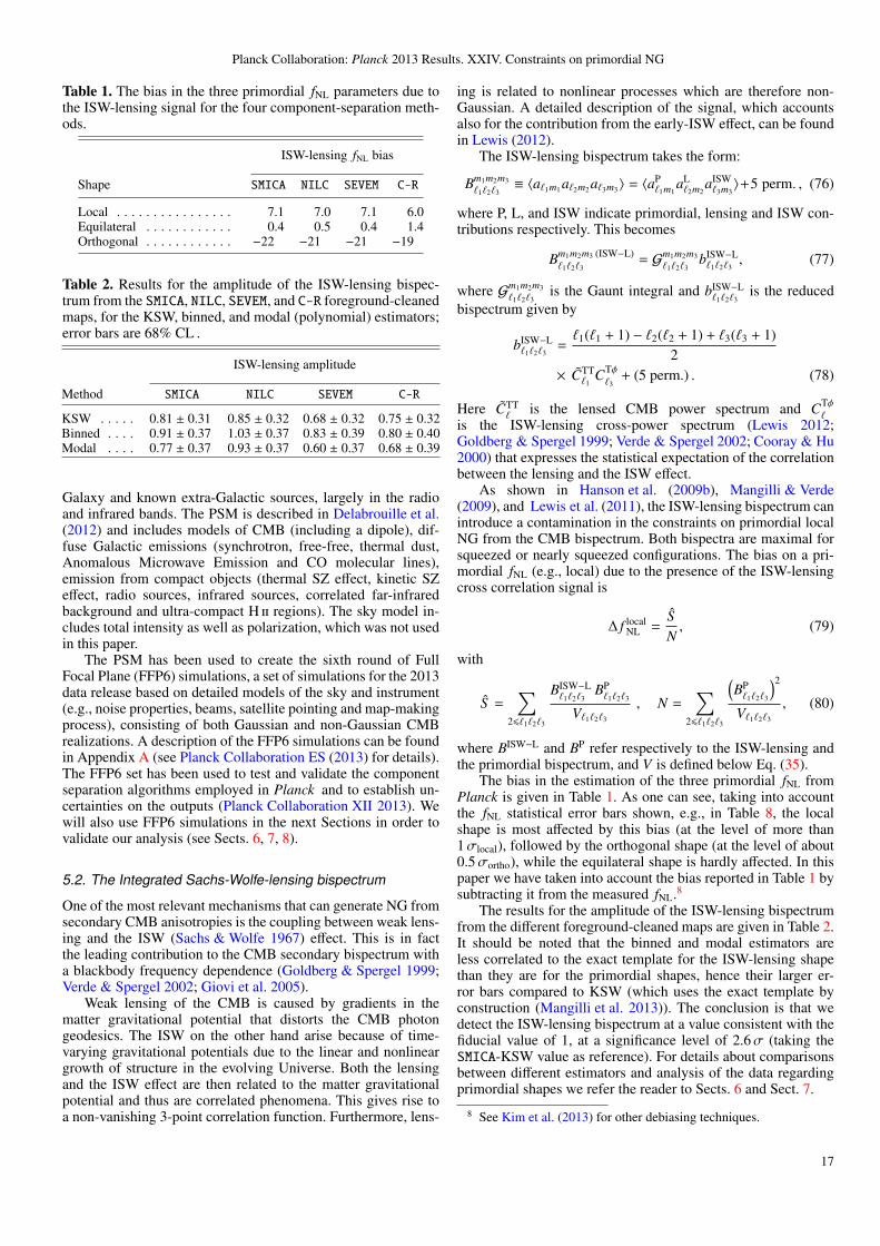
Planck Collaboration: Planck 2013 Results. XXIV. Constraints on primordial NG
Table 1. The bias in the three primordial fNL parameters due tothe ISW-lensing signal for the four component-separation meth-ods.
ISW-lensing fNL bias
Shape SMICA NILC SEVEM C-R
Local . . . . . . . . . . . . . . . . 7.1 7.0 7.1 6.0Equilateral . . . . . . . . . . . . 0.4 0.5 0.4 1.4Orthogonal . . . . . . . . . . . . −22 −21 −21 −19
Table 2. Results for the amplitude of the ISW-lensing bispec-trum from the SMICA, NILC, SEVEM, and C-R foreground-cleanedmaps, for the KSW, binned, and modal (polynomial) estimators;error bars are 68% CL .
ISW-lensing amplitude
Method SMICA NILC SEVEM C-R
KSW . . . . . 0.81 ± 0.31 0.85 ± 0.32 0.68 ± 0.32 0.75 ± 0.32Binned . . . . 0.91 ± 0.37 1.03 ± 0.37 0.83 ± 0.39 0.80 ± 0.40Modal . . . . 0.77 ± 0.37 0.93 ± 0.37 0.60 ± 0.37 0.68 ± 0.39
Galaxy and known extra-Galactic sources, largely in the radioand infrared bands. The PSM is described in Delabrouille et al.(2012) and includes models of CMB (including a dipole), dif-fuse Galactic emissions (synchrotron, free-free, thermal dust,Anomalous Microwave Emission and CO molecular lines),emission from compact objects (thermal SZ effect, kinetic SZeffect, radio sources, infrared sources, correlated far-infraredbackground and ultra-compact H ii regions). The sky model in-cludes total intensity as well as polarization, which was not usedin this paper.
The PSM has been used to create the sixth round of FullFocal Plane (FFP6) simulations, a set of simulations for the 2013data release based on detailed models of the sky and instrument(e.g., noise properties, beams, satellite pointing and map-makingprocess), consisting of both Gaussian and non-Gaussian CMBrealizations. A description of the FFP6 simulations can be foundin Appendix A (see Planck Collaboration ES (2013) for details).The FFP6 set has been used to test and validate the componentseparation algorithms employed in Planck and to establish un-certainties on the outputs (Planck Collaboration XII 2013). Wewill also use FFP6 simulations in the next Sections in order tovalidate our analysis (see Sects. 6, 7, 8).
5.2. The Integrated Sachs-Wolfe-lensing bispectrum
One of the most relevant mechanisms that can generate NG fromsecondary CMB anisotropies is the coupling between weak lens-ing and the ISW (Sachs & Wolfe 1967) effect. This is in factthe leading contribution to the CMB secondary bispectrum witha blackbody frequency dependence (Goldberg & Spergel 1999;Verde & Spergel 2002; Giovi et al. 2005).
Weak lensing of the CMB is caused by gradients in thematter gravitational potential that distorts the CMB photongeodesics. The ISW on the other hand arise because of time-varying gravitational potentials due to the linear and nonlineargrowth of structure in the evolving Universe. Both the lensingand the ISW effect are then related to the matter gravitationalpotential and thus are correlated phenomena. This gives rise toa non-vanishing 3-point correlation function. Furthermore, lens-
ing is related to nonlinear processes which are therefore non-Gaussian. A detailed description of the signal, which accountsalso for the contribution from the early-ISW effect, can be foundin Lewis (2012).
The ISW-lensing bispectrum takes the form:
Bm1m2m3`1`2`3
≡ 〈a`1m1 a`2m2 a`3m3〉 = 〈aP`1m1
aL`2m2
aISW`3m3〉+5 perm. , (76)
where P, L, and ISW indicate primordial, lensing and ISW con-tributions respectively. This becomes
Bm1m2m3 (ISW−L)`1`2`3
= Gm1m2m3`1`2`3
bISW−L`1`2`3
, (77)
where Gm1m2m3`1`2`3
is the Gaunt integral and bISW−L`1`2`3
is the reducedbispectrum given by
bISW−L`1`2`3
=`1(`1 + 1) − `2(`2 + 1) + `3(`3 + 1)
2× CTT
`1CTφ`3
+ (5 perm.) . (78)
Here CTT` is the lensed CMB power spectrum and CTφ
`is the ISW-lensing cross-power spectrum (Lewis 2012;Goldberg & Spergel 1999; Verde & Spergel 2002; Cooray & Hu2000) that expresses the statistical expectation of the correlationbetween the lensing and the ISW effect.
As shown in Hanson et al. (2009b), Mangilli & Verde(2009), and Lewis et al. (2011), the ISW-lensing bispectrum canintroduce a contamination in the constraints on primordial localNG from the CMB bispectrum. Both bispectra are maximal forsqueezed or nearly squeezed configurations. The bias on a pri-mordial fNL (e.g., local) due to the presence of the ISW-lensingcross correlation signal is
∆ f localNL =
SN, (79)
with
S =∑
26`1`2`3
BISW−L`1`2`3
BP`1`2`3
V`1`2`3
, N =∑
26`1`2`3
(BP`1`2`3
)2
V`1`2`3
, (80)
where BISW−L and BP refer respectively to the ISW-lensing andthe primordial bispectrum, and V is defined below Eq. (35).
The bias in the estimation of the three primordial fNL fromPlanck is given in Table 1. As one can see, taking into accountthe fNL statistical error bars shown, e.g., in Table 8, the localshape is most affected by this bias (at the level of more than1σlocal), followed by the orthogonal shape (at the level of about0.5σortho), while the equilateral shape is hardly affected. In thispaper we have taken into account the bias reported in Table 1 bysubtracting it from the measured fNL.8
The results for the amplitude of the ISW-lensing bispectrumfrom the different foreground-cleaned maps are given in Table 2.It should be noted that the binned and modal estimators areless correlated to the exact template for the ISW-lensing shapethan they are for the primordial shapes, hence their larger er-ror bars compared to KSW (which uses the exact template byconstruction (Mangilli et al. 2013)). The conclusion is that wedetect the ISW-lensing bispectrum at a value consistent with thefiducial value of 1, at a significance level of 2.6σ (taking theSMICA-KSW value as reference). For details about comparisonsbetween different estimators and analysis of the data regardingprimordial shapes we refer the reader to Sects. 6 and Sect. 7.
8 See Kim et al. (2013) for other debiasing techniques.
17

Planck Collaboration: Planck 2013 Results. XXIV. Constraints on primordial NG
0.00
0.04
0.08
0 500 1000 1500 2000 2500
(a)f NL ISW-L = 0.81
0.
000
0.00
2
0 500 1000 1500 2000 2500
(b)b PS = 7.7
!S
!!S
!
!
!
Fig. 2. The binned skew-C` statistics from the SMICAmap for (a)ISW-lensing and (b) Poisson point sources. Theoretical curvesare not fitted to the data shown, but are plotted with the ampli-tude (the only free parameter) determined from the KSW tech-nique. The Poisson point-source foreground is clearly detected,and the ISW-lensing skew-spectrum is evident and consistentwith the overall 2.6σ detection. bps is the Poisson point-sourceamplitude in dimensionless units of 10−29, and f ISW-L
NL is the ISW-lensing amplitude in units of that expected from the Planck best-fit cosmology. Error bars come from covariance estimates from1000 simulated maps, and the points are mildly correlated.
We show for the SMICA map in the top figure of Fig. 2the measured skew-C` spectrum (see Sect. 3.2.2) for opti-mal detection of the ISW-lensing bispectrum, along with thebest-fitting estimates of fNL from the KSW method for dif-ferent values of `. It should be noted that the skew-C` spec-trum is not a fit to the KSW data points; its shape is fullyfixed by the template under consideration, with only the over-all amplitude as a free parameter. Hence the agreement be-tween the curve and the points is good evidence that KSWis really detecting the ISW-lensing effect and not some othersource of NG. Note that point sources, at the level determinedby their own skew-spectrum, do not contribute significantlyto the ISW-lensing statistic). See Planck Collaboration XVII(2013), Planck Collaboration XIX (2013) for further informa-tion about the detection by Planck of the ISW-lensing signal.
5.3. Point-sources bispectrum
Extra-Galactic point sources at Planck frequencies are dividedinto two broad categories: radio sources with synchrotron and/orfree-free emission; and infrared galaxies with thermal emissionfrom dust heated by young stars. Radio sources are dominant atcentral CMB frequencies up to 143 GHz, and can be considered
Table 3. Results for the amplitude of the point source (Poisson)bispectrum (in dimensionless units of 10−29) from the SMICA,NILC, SEVEM, and C-R foreground-cleaned maps, for the KSW,binned, and modal (polynomial) estimators; error bars are 68%CL. Note that the KSW and binned estimators use `max = 2500,while the modal estimator has `max = 2000.
Point source bispectrum amplitude/10−29
Method SMICA NILC SEVEM C-R
KSW . . . . . . 7.7 ± 1.5 9.2 ± 1.7 7.6 ± 1.7 1.1 ± 5.1Binned . . . . 7.7 ± 1.6 8.2 ± 1.6 7.5 ± 1.7 0.9 ± 4.8Modal . . . . . 10 ± 3 11 ± 3 10 ± 3 0.5 ± 6
unclustered (Toffolatti et al. 1998; Gonzalez-Nuevo et al. 2005).Hence their bispectrum is constant and is related to their numbercounts as
bps = k3ν
∫ S c
0S 3 dn
dSdS , (81)
with S the flux density, dn/dS the number counts per steradian,S c the flux cut and kν the conversion factor from flux to relativetemperature elevation, depending on the frequency and instru-mental bandpass.
Infrared galaxies become important at higher frequencies,217GHz and above, and are highly clustered in dark matter ha-los, which enhances their bispectrum on large angular scales(Lacasa et al. 2012; Curto et al. 2013). However, in the Planckcontext it was shown by Lacasa & Aghanim (2012) that the IRbispectrum is more than 90% correlated with the Poissoniantemplate of the radio sources. So a joint estimation of fNL with aPoissonian bispectrum template will essentially account for theIR signal, and provide quasi-identical values compared to ananalysis accounting for the IR bispectrum template. Indeed, inour final optimal bispectrum constraints for primordial shapes,we will account for the potential contamination from pointsources by jointly fitting primordial and Poisson templates to thedata.
Our final measured point-source bispectrum amplitudesfrom the data are reported in Table 3. The amplitude is expressedin dimensionless units, i.e., it has been divided by the appropri-ate power of the monopole temperature T0, and has been mul-tiplied by 1029. As shown in Sect. 8.1, the Poisson template isthe only one that still evolves significantly between ` = 2000and ` = 2500. This explains the differences between the valuesof the KSW and binned (that use `max = 2500) and the modal(that uses `max = 2000) estimators. It has been shown that forthe same value of `max all three estimators agree very well.
We finally conclude from Table 3 that we detect the point-source bispectrum with high significance in the SMICA, NILC,and SEVEM cleaned maps, while it is absent from the C-R cleanedmap. The measured skew-C` spectrum of the SMICA map in thebottom figure of Fig. 2 gives further evidence that the NG fromforeground point sources is convincingly detected. The only de-gree of freedom in this plot is the amplitude, which is not set bya direct fit to the skew-C`, but rather is estimated by KSW. As aresult, the good agreement with the shape of this skew-C` spec-trum is powerful evidence that there is NG from point sources.However, this still turns out to be a negligible contaminant forprimordial fNL studies, due to the very low correlation betweenthe Poisson bispectrum and the primordial shapes.
18

Planck Collaboration: Planck 2013 Results. XXIV. Constraints on primordial NG
5.4. Non-primordial contributions to the trispectrum
The main non-instrumental source of non-primordial sig-nal is the kinematic modulation dipole due to the pecu-liar velocity of the earth, u, whose magnitude is O(10−3)(Challinor & van Leeuwen 2002; Kosowsky & Kahniashvili2011; Amendola et al. 2011). If data are used to constrainτNL using the dipole modulation (which shrinks the Fishererror by a factor of two relative to starting at L = 2), thedipole-induced signal must be subtracted, since its modulationreconstruction has signal-to-noise larger than unity at Planckresolution. Confirmation that this signal is detected with theexpected magnitude and direction is a good test of our method-ology. The dipole signal seen by Planck is studied in detailin Planck Collaboration XXVII (2013), so we only summarizethe key points here.
The local Doppler effect modulates the observed CMB tem-perature T0[1 + ∆T (n)] by 1 + n · u at leading order, so thatT (n) = T0[1 + ∆T (n)](1 + n · u). The spectrum in each directionremains a blackbody, but the relative response in the intensityIν(ν, n) at the observed Planck frequencies is however frequencydependent. The effective thermodynamic fractional temperatureanisotropy ∆Θ at each frequency for zero peculiar velocity isdefined by
Iν(ν, n) = Iν(ν)[1 +
d ln Iνd ln T
∣∣∣∣∣ν∆Θ(n)
]. (82)
With peculiar velocity the temperature T depends on the secondorder term ∆T n · u, so expanding the Planck function to secondorder then gives a change in the effective small-scale temper-ature anisotropy from both first and second order terms in theexpansion of Iν:
∆Θ(n) →[1 + n · u + T
d2Iν/dT 2
dIν/dTn · u
]∆Θ(n)
= (1 + [x coth(x/2) − 1] n · u) ∆Θ(n), (83)
where x ≡ hν/kBT0 (and we neglect small second-order non-modulation terms). Thus the anisotropies in the Planck mapshave a dipolar modulation given by 1 + bν n · u, where for the fre-quency bands we use b143 ≈ 2, b217 ≈ 3, and β ≡ |u| = 1.23×10⁻³
in the direction of CMB dipole. In addition our peculiar velocityinduces kinetic aberration, which looks at leading order exactlylike a dipole lensing convergence and only projects weakly intothe power anisotropy estimator. For constraining τNL both of theexpected kinematic signals can be included in the simulations,and hence subtracted in the mean field of the modulation recon-struction.
Secondary effects are dominated by the significant and veryblue lensing signal. However unlike for the fNL bispectrum lens-ing only overlaps with τNL at a small fraction of the error bar aslong as only low modulation multipoles L <
∼ 10 are used, wherethe τNL signal peaks (Pearson et al. 2012). We include lensing inthe simulations, so lensing is straightforwardly accounted for inour analysis by its inclusion in the N(0)
L noise bias (Eq. (72)) andmean field.
A variety of instrumental effects can also give a spuriousmodulation signal if not modelled accurately. In particular themean field due to anisotropic noise is very large (Hanson et al.2009a). On the ultra-large scales of interest for τNL, our un-derstanding of the noise is not adequate to calculate accuratelyand subtract this large signal. Instead, as for the power spec-trum estimation, we use cross-map estimators that have no noise
mean field on average. Both the noise and most other instru-mental effects such as gain variations are expected to producea signal with approximate symmetry about the ecliptic plane.Our modulation reconstruction methodology is especially use-ful here, since we can easily inspect the orientation of any sig-nal found; for example a naive treatment of the noise not usingcross-maps would give a large apparent quadrupolar modulationsignal aligned with the ecliptic, corresponding to percent-levelmisestimation of the noise mean field from inaccurate noise sim-ulation.
Beam asymmetries are included in the simulation, as de-scribed in Planck Collaboration XVII (2013), but their effectis very small, since the modulation we are reconstructing isisotropic.
Since we are reconstructing a modulation of small-scalepower, the estimator is totally insensitive to smooth large-scale foregrounds. However large-scale variation in small-scale foreground power can mimic a trispectrum modulation.We project out 857 GHz as a dust template in our inverse-variance filtering procedure, as described in Appendix A ofPlanck Collaboration XVII (2013), but do not include any otherforeground model in the trispectrum analysis. Any unmodelledforeground power variation would increase the τNL signal, so ourmodelling is sufficient to place a robust upper limit.
6. Validation Tests
The fNL results quoted in this paper have all been cross-validated using multiple bispectrum-based estimators from dif-ferent groups. Having multiple estimators was extremely usefulfor the entire analysis, for two main reasons. First, it allowedgreat improvement in the robustness of the final results. In theearly stages of the work the comparison between different in-dependent techniques helped to resolve bugs and other techni-cal issues in the various computer codes, while during the laterstages it was very useful to understand the data and find the opti-mal way of extracting information about the various bispectrumtemplates. Secondly, besides these cross-checking purposes, dif-ferent estimators provide also interesting complementary infor-mation, going beyond simple fNL estimation. For example, thebinned and modal estimators provide a reconstruction of thefull bispectrum of the data (smoothed in different domains), theskew-C` estimator allows monitoring of the contribution to fNLfrom different sources of NG, the wavelets reconstruction allowsfNL directionality tests, and so on.
In this Section we are concerned with the first point above,that is, the use of multiple bispectrum-based pipelines as a wayto improve the robustness of the results. For this purpose, a largeamount of work was dedicated to the development and analy-sis of various test maps, in order to validate the estimators. Thismeans not only checking that the various estimators recover theinput fNL within the expected errors, but also that the resultsagree on a map-by-map basis.
The Section is split into two parts. Sect. 6.1 shows results ona set of initially full-sky, noiseless, Gaussian CMB simulations,to which we add, in several steps, realistic complications, in-cluding primordial NG, anisotropic coloured noise, and a mask,showing the impact on the results at each step. In Sect. 6.2 weshow our results on a set of simulations that mimic the real dataas closely as possible (except for the presence of foregroundresiduals, which will be studied in Sect. 8.4): no primordial NG,but NG due to the ISW-lensing effect; simulated instrumentaleffects and realistic noise; and simulations passed through the
19

Planck Collaboration: Planck 2013 Results. XXIV. Constraints on primordial NG
component separation pipelines. In fact these are the FFP6 sim-ulations (see Appendix A) that are used to determine the errorbars for the final Planck results.
We present here only a small subset of the large number ofvalidation tests that were performed. For example, we also had anumber of “blind fNL challenges”, in which the different groupsreceived a simulated data set with an unknown value of inputfNL for a given shape and they had to report their estimated val-ues. In addition different noise models were tested (white vs.coloured and isotropic vs. anisotropic), leading to the conclu-sion that it is important to make the noise in the estimator cal-ibration as realistic as possible (coloured and anisotropic). Wealso tested different Galactic and point source masks, with andwithout inpainting, concluding that it is best to fill in both thepoint sources and the Galactic mask, using a sufficient numberof iterations in our diffusive procedure to entirely fill in the pointsource gaps, while at the same time only effectively apodizingthe Galactic mask (no small-scale structure in its interior). Therewere also various tests on FFP simulations of Planck data withGaussian or non-Gaussian CMB and all foregrounds, providedby the PSM (see Appendix A.4). These simulations were testedboth before and after they had passed through the componentseparation pipelines. In all comparison tests the results were con-sistent with input fNL values and differences between estimatorswere consistent with theoretical expectations.
6.1. Validation of estimators in the presence of primordialnon-Gaussianity
The aim of the first set of validation tests is threefold. First, wewant to study the level of agreement from different estimatorsin ideal conditions (i.e., full-sky noiseless data). The expectedscatter between measurements is, in this case, entirely due tothe slightly imperfect correlation between weights of estimatorsthat adopt different schemes to approximate the primordial shapetemplates. For this case the scatter can be computed analytically(see Appendix B for details). We can then verify that our resultsin ideal conditions match theoretical expectations. This is donein Sect. 6.1.1. Second, we want to make sure that the estima-tors are unbiased and correctly recover fNL in input for local,equilateral, and orthogonal shapes. This is done in Sects. 6.1.2and 6.1.3, where a superposition of local, equilateral and orthog-onal bispectra is included in the simulations and the three fNLvalues are estimated both independently and jointly. Finally wewant to understand how much the agreement between pipelinesin ideal conditions is degraded when we include a realistic cor-related noise component and a sky cut, thus requiring the intro-duction of a linear term in the estimators in order to accountfor off-diagonal covariance terms introduced by the breakingof rotational invariance. Since we want to study the impact ofadding noise and masking separately, we will first work on a setof full-sky maps with noise in Sect. 6.1.2, and then add a maskin Sect. 6.1.3.
The tests were applied to the KSW, binned and modal es-timators. These are the bispectrum pipelines used to analysePlanck data in Sect. 7. Our goal for this set of tests is not somuch to attain the tightest possible agreement between methods,as it is to address the points summarized in the above paragraph.For this reason the estimator implementations used in this spe-cific Section were slightly less accurate but faster to computethan those adopted for the final data analysis of Sect. 7. The pri-mary difference with respect to the main analysis is that a smallernumber of simulations was used to calibrate the linear term (80–100 in these tests, as against 200 or more for the full analysis).
For the modal estimator we also use a faster expansion with asmaller number of modes: 300 here versus 600 in the high ac-curacy version of the pipeline9 used in Sect. 7. Even with manyfewer modes, the modal estimator is still quite accurate: the cor-relation coefficient for the modal expansion of the local templateis 0.95, while for the equilateral and orthogonal shapes it is 0.98.
6.1.1. Ideal Gaussian simulations
As a basis for the other tests we start with the ideal case, a setof 96 simulations of a full-sky Gaussian CMB, with a Gaussianbeam with FWHM 5 arcmin and without any noise, cut off at`max = 2000 in our analyses. The independent Fisher matrix er-ror bars in that case are 4.2 for local NG, 56 for equilateral, and28 for orthogonal.
Note that this test does not make sense for all estimators, andhence results are not included for all of them. For example, forthe binned estimator the optimal binning depends on the noise.While this dependence is not very strong, the difference betweenno noise and Planck noise is sufficiently large that a completelydifferent binning would have to be used just for this test, goingagainst the purpose of this Section to validate the estimators asused for the data analysis.10
The purpose here is mostly aimed at checking consistencywith the following formula (derived in Appendix B) for the ex-pected scatter (standard deviation) between fNL results of thesame map from an exact and an approximate estimator:
σδ fNL = ∆th
√1 − r2
r. (84)
Here ∆th is the standard deviation of the exact estimator and ris the correlation coefficient that gives the correlation of the ap-proximate bispectrum template with the exact one, defined as
r ≡
∑`1≤`2≤`3
Bth`1`2`3
Bexp`1`2`3
g`1`2`3 C`1 C`2 C`3√∑`1≤`2≤`3
(Bth`1`2`3
)2
g`1`2`3 C`1 C`2 C`3
∑`1≤`2≤`3
(Bexp`1`2`3
)2
g`1`2`3 C`1 C`2 C`3
, (85)
where the label “th” denotes the initial bispectrum shape to fit tothe data, and “exp” is the approximate expanded one. Note thatthis formula has been obtained under the simplifying assump-tions of Gaussianity, full-sky coverage and homogeneous noise.For applications dealing with more realistic cases we might ex-pect the scatter to become larger, while remaining qualitativelyconsistent.
The results averaged over the whole set of maps are given inTable 4 for the KSW and modal estimators individually, as wellas for their difference. The plane wave modal expansion imple-mented here achieves about 98% correlation with the separableshapes used by KSW. According to the formula above we thenexpect a standard deviation of map-by-map differences of order
9 While most of the modal results in this paper come from the mostaccurate 600 modes pipeline, a few computationally intensive data vali-dation tests of Sect. 8 also use the fast 300 modes version; therefore theresults in this Section also provide a direct validation of the fast modalpipeline.
10 While the binning with 48 bins and `max = 2000 used in the vali-dation tests of Sects. 6.1.2 and 6.1.3 is also slightly different from thebinning used for the data analysis with 51 bins and `max = 2500, thesedifferences are very small and the binnings have very similar correlationcoefficients of 0.99 or more for local and equilateral shapes, and 0.95for orthogonal.
20

Planck Collaboration: Planck 2013 Results. XXIV. Constraints on primordial NG
Table 4. Results for fNL for the set of ideal Gaussian simulationsdescribed in Sect. 6.1.1 for the KSW and modal estimators andfor their difference, assuming all shapes to be independent.
fNL
Shape KSW Modal Modal − KSW
Local . . . . . . . . . −0.5 ± 4.1 −0.5 ± 4.1 −0.05 ± 0.63Equilateral . . . . . . 2.2 ± 48 1.3 ± 48 −0.9 ± 8.9Orthogonal . . . . . −1.1 ± 29 −1.0 ± 30 0.1 ± 6.5
0.2∆ fNL for a given shape, where ∆ fNL is the corresponding fNLerror bar. Looking at the left-hand side of Table 4, we see thatthe error bars are 4 for local NG, 50 for equilateral, and 30 fororthogonal. So we predict a standard deviation of map-by-mapdifferences of 0.8, 10 and 6 for local, equilateral, and orthogo-nal NG, respectively. As one can see from the “Modal-KSW”column, the measurements are in excellent agreement with thetheoretical expectation.
6.1.2. Non-Gaussian simulations with realistic noise
A set of 96 full-sky non-Gaussian CMB simulations was createdaccording to the process described by Fergusson et al. (2010a),with local f local
NL = 12, equilateral f equilNL = 35, and orthogonal
f orthoNL = −22. The effect of a 5 arcmin beam was added, as well
as realistic coloured and anisotropic noise according to the speci-fications of the SMICA cleaned map. The independent Fisher ma-trix error bars in that case are 5.3 for local, 63 for equilateral,and 33 for orthogonal NG, while the joint ones are respectively6.0, 64, and 37.
The results averaged over the whole set are given in Table 5for the various estimators individually, as well as for the differ-ences with respect to KSW. Compared to the previous case wenow deviate from the exact theoretical expectation for two rea-sons: we include a realistic correlated noise component; and wehave NG in the maps. The presence of NG in the input mapswill lower the agreement between estimators with respect to theGaussian case if the correlation between weights is not exactly100%. This is even more true in this specific case, where NGof three different kinds is present in the input maps and alsocross-correlation terms between different expanded shapes areinvolved (and propagated over in the joint analysis). Moreover,when noise is included the specific modal expansion used forthis test is 95% correlated to the separable KSW local shape (sothere is a 3% reduction of the correlation compared to the idealcase for the modal local shape); we thus expect a further degra-dation of the level of agreement for this specific case. Finally, inorder to correct for noise effects, a linear term has to be addedto the estimators. Since the linear term is obtained by MC aver-aging over just 80 or 96 simulations in this test (depending onthe estimator), MC errors are also adding to the measured differ-ences. Of course the MC error can be reduced by increasing thenumber of simulations in the linear term sample. We do this forthe analysis of the real data and in Sect. 6.2, but it was computa-tionally too expensive for this set of preliminary validation tests,so we decided here to just account for it in the final interpretationof the results.
As a consequence of the above, we can no longer expect themap-by-map fNL differences to follow perfectly the theoreticalexpectation, obtained in the previous Section in idealized con-ditions (full-sky, no noise, and Gaussianity). With these caveats
in mind, the agreement between different pipelines remains verygood, being about 0.3σ in most cases and about 0.5σ for themodal-KSW difference in the local case, which can be easily ex-plained by the fact that this is the set of weights with the lowestcorrelation (95%, as mentioned above). All estimators are unbi-ased and recover the correct input values.
6.1.3. Impact of the mask
To the simulations of Sect. 6.1.2 we now apply the Planckunion mask - denoted U73 - masking both the Galaxy andthe brightest point sources and leaving 73% of the sky un-masked (Planck Collaboration XII 2013). This is the same maskused to analyse Planck data in Sect. 7. The independent Fishermatrix error bars in that case (taking into account the fsky cor-rection) are 6.2 for local NG, 74 for equilateral, and 39 for or-thogonal, while the joint ones are respectively 7.1, 76, and 44.
All masked areas of the sky (both Galactic and point sources)are filled in with a simple iterative method. In this simple in-painting method each pixel in the mask is filled with the averageof all eight surrounding pixels, and this is repeated 2000 timesover all masked pixels. The filling-in helps to avoid propagatingthe effect of a sharp edge and the lack of large-scale power insidethe mask to the unmasked regions during harmonic transforms.This inpainting method is the one that was used to produce allNG results in this paper for methods that need it (KSW, binnedand modal).
The results averaged over the whole set of simulations aregiven in Table 6 for the various estimators individually, as wellas for the differences with respect to KSW. The map-by-mapresults are shown in Fig. 3.
This is the most realistic case we consider in this set of tests.Besides noise, we also include a sky cut and our usual mask in-painting procedure. All the caveats mentioned for the previouscase are still valid, and possibly emphasized by the inclusion ofmask and inpainting. In the light of this, the agreement is stillvery good, worsening a bit with respect to the “full-sky + noise”case only for the local measurement, where the mask is indeedexpected to have the biggest impact. In the joint analysis all esti-mators recover the correct input values for the local and orthog-onal cases, but all estimators find a value for equilateral NG thatis somewhat too low. It is unclear whether this is an effect ofmasking and inpainting on the equilateral measurement or just astatistical fluctuation for this set of simulations. In any case, thispotential bias is small compared to the statistical uncertainty, sothat it would not have a significant impact on the final results.
To summarize the results of this Sect. 6.1, we performed anextensive set of validation tests between different fNL estimatorsusing strongly, but not perfectly, correlated primordial NG tem-plates in their weights. The test consisted in comparing the fNLmeasured by the different estimators for different sets of simula-tions, on a map-by-map basis. We started from ideal conditions:full-sky Gaussian noiseless maps. In this case we computed atheoretical formula providing the expected standard deviation ofthe fNL differences, as a function of the correlations between theinput NG templates in the different estimators. Our results matchthis formula very well. In the other two simulation sets we addedrealistic features (noise, mask and inpainting) and we includeda linear combination of local, equilateral and orthogonal NG.First of all we verified that all the pipelines correctly recoverthe three fNL input values, hence they are unbiased. Moreover,we observed that adding such features produces an expectedslight degradation of the level of agreement between differentpipelines, that nevertheless remains very good: about 0.3–0.4σ
21
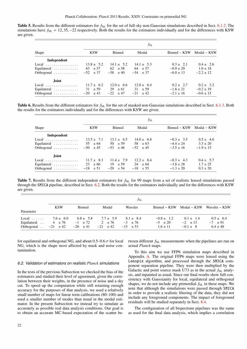
Planck Collaboration: Planck 2013 Results. XXIV. Constraints on primordial NG
Table 5. Results from the different estimators for fNL for the set of full-sky non-Gaussian simulations described in Sect. 6.1.2. Thesimulations have fNL = 12, 35,−22 respectively. Both the results for the estimators individually and for the differences with KSWare given.
fNL
Shape KSW Binned Modal Binned − KSW Modal − KSW
IndependentLocal . . . . . . . . . . . . . . . . 13.8 ± 5.2 14.1 ± 5.2 14.1 ± 5.3 0.3 ± 2.1 0.4 ± 2.6Equilateral . . . . . . . . . . . . 63 ± 57 62 ± 58 64 ± 57 −0.9 ± 20 1.0 ± 18Orthogonal . . . . . . . . . . . . −52 ± 37 −58 ± 40 −54 ± 37 −6.0 ± 13 −2.2 ± 12
JointLocal . . . . . . . . . . . . . . . . 11.7 ± 6.2 12.0 ± 6.6 12.0 ± 6.4 0.2 ± 2.7 0.2 ± 3.2Equilateral . . . . . . . . . . . . 31 ± 59 29 ± 61 31 ± 59 −1.8 ± 21 −0.2 ± 19Orthogonal . . . . . . . . . . . . −20 ± 43 −22 ± 47 −21 ± 42 −2.1 ± 16 −0.6 ± 15
Table 6. Results from the different estimators for fNL for the set of masked non-Gaussian simulations described in Sect. 6.1.3. Boththe results for the estimators individually and for the differences with KSW are given.
fNL
Shape KSW Binned Modal Binned − KSW Modal − KSW
IndependentLocal . . . . . . . . . . . . . . . . 13.5 ± 7.1 13.1 ± 6.5 14.0 ± 6.8 −0.3 ± 3.5 0.5 ± 4.6Equilateral . . . . . . . . . . . . 55 ± 64 50 ± 59 58 ± 63 −4.4 ± 24 3.3 ± 20Orthogonal . . . . . . . . . . . . −50 ± 45 −53 ± 46 −52 ± 45 −3.5 ± 16 −1.9 ± 15
JointLocal . . . . . . . . . . . . . . . . 11.7 ± 8.3 11.4 ± 7.9 12.2 ± 8.4 −0.3 ± 4.3 0.4 ± 5.7Equilateral . . . . . . . . . . . . 23 ± 66 19 ± 59 24 ± 64 −3.8 ± 28 1.7 ± 25Orthogonal . . . . . . . . . . . . −18 ± 51 −20 ± 54 −18 ± 55 −1.3 ± 20 0.3 ± 20
Table 7. Results from the different independent estimators for fNL for 99 maps from a set of realistic lensed simulations passedthrough the SMICA pipeline, described in Sect. 6.2. Both the results for the estimators individually and for the differences with KSWare given.
fNL
KSW Binned Modal Wavelet Binned − KSW Modal − KSW Wavelet − KSWParameter
Local . . . . . . 7.6 ± 6.0 6.8 ± 5.8 7.7 ± 5.9 8.1 ± 8.4 −0.8 ± 1.2 0.1 ± 1.4 0.5 ± 6.4Equilateral . . 4 ± 76 −1 ± 72 2 ± 76 −3 ± 76 −5 ± 20 −2 ± 13 −7 ± 91Orthogonal . . −21 ± 42 −20 ± 41 −21 ± 42 −15 ± 53 1.6 ± 11 −0.1 ± 8 6.4 ± 48
for equilateral and orthogonal NG, and about 0.5–0.6σ for localNG, which is the shape most affected by mask and noise con-tamination.
6.2. Validation of estimators on realistic Planck simulations
In the tests of the previous Subsection we checked the bias of theestimators and studied their level of agreement, given the corre-lation between their weights, in the presence of noise and a skycut. To speed up the computation while still retaining enoughaccuracy for the purposes of that analysis, we used a relativelysmall number of maps for linear term calibrations (80–100) andused a smaller number of modes than usual in the modal esti-mator. In the present Subsection we instead try to simulate asaccurately as possible real data analysis conditions. Our goal isto obtain an accurate MC-based expectation of the scatter be-
tween different fNL measurements when the pipelines are run onactual Planck maps.
To this aim we use FFP6 simulation maps described inAppendix A. The original FFP6 maps were lensed using theLenspix algorithm, and processed through the SMICA com-ponent separation pipeline. They were then multiplied by theGalactic and point source mask U73 as in the actual fNL analy-sis, and inpainted as usual. Since our final results show full con-sistency with Gaussianity for local, equilateral and orthogonalshapes, we do not include any primordial fNL in these maps. Wenote that although the simulations were passed through SMICAin order to provide a realistic filtering of the data, they did notinclude any foreground components. The impact of foregroundresiduals will be studied separately in Sect. 8.4.
The configuration of all bispectrum pipelines was the sameas used for the final data analysis, which implies a correlation
22

Planck Collaboration: Planck 2013 Results. XXIV. Constraints on primordial NG
20 40 60 80
Map number
−2
0−
10
01
02
03
04
0
flo
cal
NL
KSW
Binned
Modal
20 40 60 80
Map number
−1
00−
50
05
01
00
15
02
00
25
0
feq
uil
NL
KSW
Binned
Modal
20 40 60 80
Map number
−2
00−
15
0−
10
0−
50
05
01
00
for
tho
NL
KSW
Binned
Modal
Fig. 3. Map-by-map comparison of the results from the differ-ent estimators for local (top), equilateral (centre), and orthogo-nal (bottom) fNL for the set of masked non-Gaussian simulationsdescribed in Sect. 6.1.3, assuming the shapes to be independent.The horizontal solid line is the average value of all maps forKSW, and the dashed and dotted horizontal lines correspond to1σ and 2σ deviations, respectively.
of 99% or better between the weights of the KSW, binned andmodal estimators. Linear terms were calibrated using 200 sim-
20 40 60 80
Map number
−1
5−
10−
50
51
01
52
02
53
0
flo
cal
NL
KSW
Binned
Modal
Wavelet
20 40 60 80
Map number
−3
00−
20
0−
10
00
10
02
00
30
0
feq
uil
NL
KSW
Binned
Modal
Wavelet
20 40 60 80
Map number
−1
50−
10
0−
50
05
01
00
15
0
for
tho
NL
KSW
Binned
Modal
Wavelet
Fig. 4. Map-by-map comparison of the results from the differ-ent estimators for local (top), equilateral (centre), and orthogonal(bottom) fNL for 99 maps from a set of realistic lensed simula-tions passed through the SMICA pipeline, described in Sect. 6.2,assuming the shapes to be independent. The horizontal solid lineis the average value of the maps for KSW, and the dashed anddotted horizontal lines correspond to 1σ and 2σ deviations, re-spectively.
23

Planck Collaboration: Planck 2013 Results. XXIV. Constraints on primordial NG
ulations, after verifying that this number allows accurate con-vergence for all the shapes. For this test we also included thewavelet bispectrum pipeline described in Sect. 3. Although thislast estimator turns out to be about 30% suboptimal and, in itscurrent implementation, less correlated with the primordial tem-plates than the other estimators, it does provide an additionalinteresting cross-check of our results by introducing another de-composition basis. We thus used it to analyse SMICA data inSect. 7, while the other three pipelines were used on all maps.
A comparison of the measured fNL map-by-map for allshapes and estimators is shown in Fig. 4. As an overall figure ofmerit of the level of agreement achieved by different pipelineswe take as usual the standard deviation of the map-by-map fNLdifferences, σδ fNL
. Table 7 shows that the final agreement be-tween the three optimal pipelines (KSW, binned, and modal) isclose to saturating the ideal bound in Eq. (84) determined by theimperfect correlation of the weights, i.e., it varies from aboutonce to twice σδ fNL
' 0.15 ∆ fNL for an r = 0.99 correlation. Thisis very consistent with the level of agreement that we find be-tween estimators for the final results from the data, providing agood indication that no spurious NG features are present in theactual data set when compared to our simulations. It should benoted that we found a similarly good level of agreement betweenestimators for the non-primordial shapes of point sources andISW-lensing, although we chose not to present those results herein order to focus on the primordial shapes. Finally, regarding thewavelet pipeline, the lower weight correlation and suboptimalerror bars produce an expected larger scatter when compared tothe other estimators. Nonetheless, the level of agreement is stillof order 1σ, which is quite acceptable for consistency checks ofthe optimal results. Again, this MC expectation agrees with whatwe see in our results on the real data.
7. Results
For our analysis of Planck data we considered foreground-cleaned maps obtained with the four component separationmethods SMICA, NILC, SEVEM, and C-R. For each map, fNLamplitudes for the local, equilateral, and orthogonal primordialshapes have been measured using three (four for SMICA) bispec-trum estimators described in Sect. 3. The results can be foundin Sect. 7.1. These estimators, as explained earlier, basically usean expansion of the theoretical bispectrum templates in differentdomains, and truncate the expansion when a high level of corre-lation with the primordial templates is achieved. These accuratedecompositions, which are highly correlated with each other, arethen matched to the data in order to extract fNL. The differentexpansions are all different implementations of the maximum-likelihood estimator given in Eq. (32). So the final estimates areall expected to be optimal, and measure fNL from nearly identi-cal fitting templates. As discussed and tested in detail on simu-lations in Sect. 6, central fNL values from different methods areexpected to be consistent with each other within about 0.3σ fNL .It is then clear that comparing outputs from both different esti-mators and different component separation methods, as we do,allows for stringent internal consistency checks and improvedrobustness of the final fNL results.
In addition, the binned and modal techniques produce shape-independent full bispectrum reconstructions in their own differ-ent domains. These reconstructions, discussed in Sect. 7.2, com-plement the standard fNL measurements in an important way,since they allow detection of possible NG features in the three-point function of the data that do not correlate significantly withthe standard primordial shapes. This advantage is shared by the
Table 8. Results for the fNL parameters of the primordial local,equilateral, and orthogonal shapes, determined by the KSW es-timator from the SMICA foreground-cleaned map. Both indepen-dent single-shape results and results marginalized over the pointsource bispectrum and with the ISW-lensing bias subtracted arereported; error bars are 68% CL . The final reported results ofthe paper are shown in bold face.
fNL(KSW)
Shape & Method Independent ISW-lensing subtracted
SMICALocal . . . . . . . . . 9.8 ± 5.8 2.7 ± 5.8Equilateral . . . . . −37 ± 75 −42 ± 75Orthogonal . . . . . −46 ± 39 −25 ± 39
skew-C` method, also applied to the data. A detection of suchfeatures would either produce a warning that some residual spu-rious NG effects are still present in the data or provide an in-teresting hint of “non-standard” primordial NG that is not cap-tured by the local, equilateral and orthogonal shapes. Additionalconstraints for a broad range of specific models are providedin Sect. 7.3 (see also Sect. 2.3). In Sect. 7.4 we present theconstraints on local NG obtained with Minkowski Functionals.Finally, in Sect. 7.5 we present our CMB trispectrum results.
7.1. Constraints on local, equilateral and orthogonal fNL
Our goal here is to investigate the standard separable local, equi-lateral and orthogonal templates used e.g., in previous WMAPanalyses (see e.g., Bennett et al. 2012). When using the modal,binned, or wavelet estimator, these theoretical templates are ex-panded approximately (albeit very accurately) using the relevantbasis functions or bins. On the other hand, the KSW estimator byconstruction works with the exact templates and, for this reason,it is chosen as the baseline to provide the final fNL results forthe standard shapes (local, equilateral, orthogonal), see Table 8.However, both the binned and modal estimators achieve opti-mal performance and an extremely high correlation for the stan-dard templates (∼ 99%), so they are statistically equivalent toKSW, as demonstrated in the previous section. This means thatwe can achieve a remarkable level of cross-validation for ourPlanck NG results. We will be able to present consistent con-straints for the local, equilateral and orthogonal models for allfour Planck foreground-cleaned maps, using three independentoptimal estimators (refer to Table 9). Regarding component sep-aration methods, we adopt the SMICA map as the default for thefinal KSW results given its preferred status among foreground-separation techniques in Planck Collaboration XII (2013). Theother component separation maps will be used for importantcross-validation of our results and to evaluate potential sensi-tivity to foreground residuals.
All the results presented in this Section were obtained usingthe union mask U73, which leaves 73% of the sky unmasked.The mask is the union of the confidence masks of the four differ-ent component separation methods, where each confidence maskdefines the region where the corresponding CMB cleaning istrusted (see Planck Collaboration XII 2013). As will be shownin Sect. 8.2, results are robust to changes that make the masklarger, but choosing a significantly smaller mask would leavesome NG foreground contamination. For the linear term CMB
24

Planck Collaboration: Planck 2013 Results. XXIV. Constraints on primordial NG
Table 9. Results for the fNL parameters of the primordial local, equilateral, and orthogonal shapes, determined by the KSW, binnedand modal estimators from the SMICA, NILC, SEVEM, and C-R foreground-cleaned maps. Both independent single-shape results andresults marginalized over the point source bispectrum and with the ISW-lensing bias subtracted are reported; error bars are 68%CL . Final reported results of the paper are shown in bold.
fNL
Independent ISW-lensing subtractedShape KSW Binned Modal KSW Binned Modal
SMICALocal . . . . . . . . . . . . . . . . 9.8 ± 5.8 9.2 ± 5.9 8.3 ± 5.9 2.7 ± 5.8 2.2 ± 5.9 1.6 ± 6.0Equilateral . . . . . . . . . . . . −37 ± 75 −20 ± 73 −20 ± 77 −42 ± 75 −25 ± 73 −20 ± 77Orthogonal . . . . . . . . . . . . −46 ± 39 −39 ± 41 −36 ± 41 −25 ± 39 −17 ± 41 −14 ± 42
NILCLocal . . . . . . . . . . . . . . . . 11.6 ± 5.8 10.5 ± 5.8 9.4 ± 5.9 4.5 ± 5.8 3.6 ± 5.8 2.7 ± 6.0Equilateral . . . . . . . . . . . . −41 ± 76 −31 ± 73 −20 ± 76 −48 ± 76 −38 ± 73 −20 ± 78Orthogonal . . . . . . . . . . . . −74 ± 40 −62 ± 41 −60 ± 40 −53 ± 40 −41 ± 41 −37 ± 43
SEVEMLocal . . . . . . . . . . . . . . . . 10.5 ± 5.9 10.1 ± 6.2 9.4 ± 6.0 3.4 ± 5.9 3.2 ± 6.2 2.6 ± 6.0Equilateral . . . . . . . . . . . . −32 ± 76 −21 ± 73 −13 ± 77 −36 ± 76 −25 ± 73 −13 ± 78Orthogonal . . . . . . . . . . . . −34 ± 40 −30 ± 42 −24 ± 42 −14 ± 40 −9 ± 42 −2 ± 42
C-RLocal . . . . . . . . . . . . . . . . 12.4 ± 6.0 11.3 ± 5.9 10.9 ± 5.9 6.4 ± 6.0 5.5 ± 5.9 5.1 ± 5.9Equilateral . . . . . . . . . . . . −60 ± 79 −52 ± 74 −33 ± 78 −62 ± 79 −55 ± 74 −32 ± 78Orthogonal . . . . . . . . . . . . −76 ± 42 −60 ± 42 −63 ± 42 −57 ± 42 −41 ± 42 −42 ± 42
Table 10. Results for the fNL parameters of the primordial local,equilateral, and orthogonal shapes, determined by the subopti-mal wavelet estimator from the SMICA foreground-cleaned map.Both independent single-shape results and results marginalizedover the point source bispectrum and with the ISW-lensing biassubtracted are reported; error bars are 68% CL. As explained inthe text, our current wavelets pipeline performs slightly worse interms of error bars and correlation to primordial templates thanthe other bispectrum estimators, but it still provides a useful in-dependent cross-check of other techniques.
fNL(wavelets)
Shape Independent ISW-lensing subtracted
SMICALocal . . . . . . . . . 10 ± 8.5 0.9 ± 8.5Equilateral . . . . . 89 ± 84 90 ± 84Orthogonal . . . . . −73 ± 52 −45 ± 52
and noise calibration, and error bar determination, we used setsof realistic FFP6 maps that include all steps of data processing,and have realistic noise and beam properties (see Appendix A).The simulations were also lensed using the Lenspix algorithmand filtered through the component separation pipelines.
In Table 8 we show results for the combination of the KSWestimator and the SMICA map, at a resolution of `max = 2500.We present both “independent” single-shape results and “ISW-lensing subtracted” ones. The former are obtained by directlyfitting primordial templates to the data. For the latter, two ad-ditional operations have been performed. In the first place, asthe name indicates, they have been corrected by subtractingthe bias due to the correlation of the primordial bispectra tothe late-time ISW-lensing contribution (Mangilli & Verde 2009;
Junk & Komatsu 2012; Hanson et al. 2009b, see Sect. 5.2). Inaddition, a joint fit of the primordial shape with the (Poissonian)point-source bispectrum amplitude extracted from the datahas been performed on the results marked “ISW-lensing sub-tracted”.11 Since the ISW-lensing bispectrum is peaked onsqueezed configurations, its impact is well known to be largestfor the local shape. The ISW-lensing bias is also important fororthogonal measurements (there is a correlation coefficient r ∼−0.5 between the local and orthogonal CMB templates), whileit is very small in the equilateral limit. The values of the ISW-lensing bias we subtract, summarized in Table 1, are calculatedassuming the Planck best-fit cosmological model as our fidu-cial model. The same fiducial parameters were of course consis-tently used to compute the theoretical bispectrum templates andthe estimator normalization. Regarding the point source contam-ination, we detect a Poissonian bispectrum at high significancein the SMICA map, see Sect. 5.3. However, marginalizing overpoint sources has negligible impact on the final primordial fNLresults, because the Poisson bispectrum template has very smallcorrelations with all the other shapes.
In light of the discussion at the beginning of this section, wetake the numbers from the KSW SMICA analysis in Table 8 as thefinal local, equilateral and orthogonal fNL constraints for the cur-rent Planck data release. These results clearly show that no evi-dence of NG of the local, equilateral or orthogonal type is foundin the data. After ISW-lensing subtraction, all fNL for the threeprimordial shapes are consistent with 0 at 68% CL. Note thatthese numbers have been cross-checked using two completelyindependent KSW pipelines, one of which is an extension toPlanck resolution of the pipeline used for the WMAP analysis(Bennett et al. 2012).
11 More precisely, in the subtracted ISW-lensing results the equilateraland orthogonal primordial shapes are also fitted jointly, although thishas a nearly negligible impact on the final result because the two shapesare by construction nearly perfectly uncorrelated.
25

Planck Collaboration: Planck 2013 Results. XXIV. Constraints on primordial NG
-1.5
-0
.5
0.5
1.5
0 500 1000 1500 2000 2500
f NL loc = 9.8
(a)
-0
.4
0.0
0.4
0 500 1000 1500 2000 2500
(b)
f NL eq = < 37
-1
.5
-0.5
0.
5
0 500 1000 1500 2000 2500
f NL orth = < 46.
(c)
!S
!/10
!3
!
!S
!/10
!4
!
!S
!/10
!4
!
Fig. 5. Binned skew-C` statistics from the SMICA map for (a) lo-cal, (b) equilateral, and (c) orthogonal. Theoretical curves arenot fitted to the data shown, but are plotted with the amplitude(the only free parameter) determined from the KSW technique.There is no evidence for detection of primordial NG. Error barsare derived from the covariance of estimates from 1000 simu-lations. There are mild correlations between data points in allfigures, but very strong correlations at high ` in the local case,reaching correlation coefficients r > 0.99 for ` > 1750.
Unlike other methods, the KSW technique is not designedto provide a reconstruction of the full bispectrum of the data.However, the related skew-C` statistic described in Sect. 3.2.2allows, for each given shape, visualization and study of the con-tribution to the measured fNL from separate `-bins. This is a use-ful tool to study potential spurious NG contamination in the data.We show for the SMICA map in Fig. 5 the measured skew-C`
spectrum for optimal detection of primordial local, equilateraland orthogonal NG, along with the best-fitting estimates of fNLfrom the KSW method. Contrary to the case of the point sourceand ISW-lensing foregrounds (see Sect. 5), the skew-C` statisticsdo not show convincing evidence for detection of the primordialshapes, suggesting that these primordial effects are not signifi-cant sources of the NG in the map. Again, point sources con-tribute very little to this statistic; ISW-lensing contributes, butonly a small fraction of the amplitude.
As mentioned before, our analysis went beyond the sim-ple application of the KSW estimator to the SMICA map. AllfNL pipelines developed for Planck analysis were applied to allcomponent-separated maps by SMICA, NILC, SEVEM, and C-R.We found from simulations in the previous Sections that theKSW, binned, and modal pipelines saturate the Cramer-Raobound, while the wavelet estimator in its current implementa-tion provides slightly suboptimal results. Wavelets remain how-ever a useful cross-check of the other methods, also given sometechnical complementarities, e.g., they are the only approach thatdoes not require inpainting, as explained in Sect. 3. Hence we in-
clude wavelet results, but only for SMICA. The fNL results for theoptimal KSW, binned and modal bispectrum estimators, for thefour component separation methods, are summarized in Table 9,one of the main products of our analysis of Planck data. Thewavelet bispectrum analysis of SMICA is reported in Table 10.In the analysis, the KSW and binned bispectrum estimators con-sidered multipoles up to `max = 2500, while the modal estimatorwent to `max = 2000. As shown in Sect. 8.1 and Table 16, er-ror bars and central values for the three primordial shapes haveconverged at `max = 2000, so the final primordial fNL estimatesfrom the three pipelines are directly comparable.12
The binned bispectrum estimator used 51 bins, which weredetermined by optimizing the expected variance of the differ-ent fNL parameters, focusing in particular on the primordialshapes.13 The modal estimator employed a polynomial basis(nmax = 600) previously described in Fergusson et al. (2010a),but augmented with a local shape mode (approximating theSW large-angle local solution) to improve convergence in thesqueezed limit. The above choices for the binned and modalmethods produce a very high correlation (generally 99% or bet-ter) of the expanded/binned templates with the exact ones usedby the KSW estimator. The wavelet estimator is based on third-order statistics generated by the different possible combinationsof the wavelet coefficient maps of the SMHW evaluated at cer-tain angular scales. See for example Antoine & Vandergheynst(1998) and Martınez-Gonzalez et al. (2002) for detailed infor-mation about this wavelet. We considered a set of 15 scaleslogarithmically spaced between 1.3 and 956.3 arcmin and wealso included the unconvolved map. The wavelet map w(Ri; b)(Eq. (60)) for each angular scale Ri has an associated extendedmask generated from the mask U73 following the procedure de-scribed and extensively used in Curto et al. 2009b,a, 2011a,b,2012; Donzelli et al. 2012; Regan et al. 2013. The wavelet coef-ficient maps are later combined into the third-order moments qi jk(Eq. (59)), for a total 816 different statistics, and these statisticsare used to constrain fNL through a χ2 test.
The high level of agreement between results from the KSW,binned and modal fNL estimators, and from all the componentseparation pipelines, is representative of the robustness of ourresults with respect to residual foreground contamination, andis fully consistent with our preliminary MC analysis shown inSect. 6. The scatter with wavelets is a bit larger, but this wasexpected due to the suboptimality of the wavelet estimator andis also in agreement with our MC expectations from the tests.Therefore wavelets do provide another successful cross-check.
7.2. Bispectrum reconstruction
As previously explained (see Sect. 3), in addition to looking inspecific bispectrum-space directions and extracting the singlenumber fNL for given shapes, the binned and modal pipelineshave the capability to generate a smoothed (i.e., either coarse-grained in `-space, or truncated at a given expansion eigen-mode) reconstruction of the full bispectrum of the data. See alsoPlanck Collaboration XXIII (2013).
12 The lower `max for the modal pipeline is also a conservative choicein view of the large survey of “non-standard” models that will be pre-sented in Sect. 7.3
13 The boundary values of the bins are: 2, 4, 10, 18, 27, 39, 55, 75, 99,130, 170, 224, 264, 321, 335, 390, 420, 450, 518, 560, 615, 644, 670,700, 742, 800, 850, 909, 950, 979, 1005, 1050, 1110, 1150, 1200, 1230,1260, 1303, 1346, 1400, 1460, 1510, 1550, 1610, 1665, 1725, 1795,1871, 1955, 2091, 2240, and 2500 (i.e., the first bin is [2,3], the second[4,9], etc., while the last one is [2240,2500]).
26

Planck Collaboration: Planck 2013 Results. XXIV. Constraints on primordial NG
7.2.1. Modal bispectrum reconstruction
The modal pipeline was applied to the Planck temperaturemaps for the foreground-separation techniques SMICA, NILC,and SEVEM (Fergusson et al. 2010a). For this analysis we usedtwo alternative sets of hybrid basis functions in order to cross-check results and identify particular signals. First, we employedtrigonometric functions (nmax = 300) augmented with the SWlocal mode, together with the three separable modes contribut-ing to the CMB ISW-lensing signal. Secondly, we employed thesame polynomial basis (nmax = 600) with local SW mode as wasused for fNL estimation.
The modal coefficients βRn extracted from the Planck SMICA,
NILC, and SEVEM maps are shown in Fig. 9. Here we have usedthe hybrid Fourier modes with local and ISW-lensing modes.These amplitudes show remarkable consistency between the dif-ferent maps, demonstrating that the alternative foreground sepa-ration techniques do not appear to be introducing spurious NG.Note that here the βR
n coefficients are for the orthonormalizedmodes Rn (Eq. (63)) and they have a roughly constant variance,so anomalously large modes can be easily identified. It is ev-ident, for example, that among the low modes there are largesignals, which include the ISW-lensing signal and point sourcecontributions.
Using the modal expansion of Eq. (45) with Eq. (63), wehave reconstructed the full 3D Planck bispectrum. This is illus-trated in Fig. 6, where we show “tetrapyd” comparisons betweendifferent foreground cleaned maps. The tetrapyd (see Fig. 1) isthe region defined by the multipoles that obey the triangle condi-tion, with ` ≤ `max. The 3D plots show the reduced bispectrum ofthe map, divided by a Sachs-Wolfe CMB bispectrum solution fora constant primordial shape, S (k1, k2, k3) = 1. This constant pri-mordial bispectrum template normalizaton is carried out in orderto remove an ∼ `4 scaling from the starting bispectrum (it is anal-ogous to multiplication of the power spectrum by `(` + 1)). Tofacilitate the interpretation of 3D bispectrum figures, note thatsqueezed configurations lie on the edges of the tetrapyd, flat-tened on the faces and equilateral in the interior, with b``` on thediagonal. The colour levels are equally spaced with red denot-ing positive values, and blue denoting negative. Given the cor-respondence of the βR
n coefficients for SMICA, NILC, and SEVEM,the reconstructed 3D signals also appear remarkably consistent,showing similar contours out to ` . 1500. At large multipoles `approaching `max = 2000, there is increased randomness in thereconstruction due to the rise in experimental noise and someevidence for a residual point source contribution.
There are some striking features evident in the 3D bispec-trum reconstruction which appear in both Fourier and polyno-mial representations, as shown in more detail in Fig. 7. There isan apparent oscillation at low ` . 500 already seen in WMAP-7(Fergusson et al. 2012). Beyond out to ` ∼ 1200 there are furtherdistinct features (mostly “flattened” on the walls of the tetrapyd),and an oscillating ISW-lensing contribution can be discerned inthe squeezed limit. For comparison, the bispectrum reconstruc-tion for one of the lensed Gaussian simulations described in sec.6.2 is shown in Fig. 8. ISW-lensing oscillating signatures in thesqueezed limit are visible also in this case. When comparing re-sults from a single simulation to the data, it is however alwaysuseful to keep in mind that the observed tetrapyd pattern is quiterealization dependent, since full bispectrum reconstructions arenoisy. Whatever its origin, Gaussian or otherwise, Fig. 7 revealsthe CMB bispectrum of our Universe as observed by Planck.
The cumulative sum F2NL over the squared orthonormal co-
efficients βRn
2 from Eq. (64) for the Planck data is illustrated
in Fig. 10 (upper panel). The Planck bispectrum contributioncan be directly compared with Gaussian expectations averagedfrom 200 lensed Gaussian maps with simulated residual fore-grounds. It is interesting to note that the integrated bispectrumsignal fairly consistently exceeds the Gaussian mean by around2σ over much of the domain. This includes the ISW and PS con-tributions for which subtraction only has a modest effect. Alsoshown (lower panel) is the corresponding cumulative F2
NL quan-tity as a function of multipole `, for which features have visiblecounterparts at comparable ` in Fig. 7. Despite the high bispec-trum signal, this χ2-test over the orthonormal mode coefficientsβR
n is cumulatively consistent with Gaussianity for each of thethree component separation methods considered. It is howeverimportant to stress that this is a model independent integratedmeasurement of NG. Fitting the data with specific bispectrumtemplates can of course enhance the signal-to-noise ratio forgiven models, especially in light of the 1 to 2 σ excess withrespect to the Gaussian expectation, shown in the lower panel.This measurement is thus not in disagreement with detection ofa residual point source (Poisson) bispectrum in the same maps(see Table 3), or with the results shown in our feature models sur-vey of Section 7.3.3. We also note some differences in the highmode region between SEVEM and the other two methods, withthe SEVEM results being closer to the Gaussian expectation. Thisis consistent with tests on simulations and with SEVEM measur-ing a slightly lower ISW-lensing amplitude than the other meth-ods (see Table 2). On the other hand the discrepancies are wellwithin statistical bounds, as it can be seen by comparing themto the Gaussian standard deviation from simulations (red line).We thus conclude that, even accounting for these high modesdeviations, the different component separation methods displaya good level of internal consistency. It is also important to noticethat this already good level of agreement becomes even strongerin “non-blind” fNL measurements, when primordial bispectrumtemplates are fit to the data, and specific theoretically relevant re-gions of the tetrapyd are selected. This can be clearly seen fromTable 9.
7.2.2. Binned bispectrum reconstruction
As explained in Sect. 3.4.2, it is interesting to study the smoothedobserved bispectrum divided by its expected standard devia-tion, since this will indicate if there is a significant deviationfrom Gaussianity for certain regions of `-space. This quantity isshown in Figs. 11 and 12 as a function of `1 and `2, for twodifferent values (or rather, bins) of `3: the intermediate value[610,654] in Fig. 11 and the high value [1330,1374] in Fig. 12.Each figure shows the results for the SMICA, NILC, SEVEM, andC-R cleaned maps as well as for the raw 143 GHz channel map.For comparison, the result for one of the lensed Gaussian simula-tions described in Sect. 6.2 is also shown. The bispectra were ob-tained with the binned bispectrum estimator and smoothed witha Gaussian kernel as explained in Sect. 3.4.2. Very blue or redregions indicate significant NG, regions that are less red or bluejust represent expected fluctuations of a Gaussian distribution.
From Fig. 11 at an intermediate value of `3 we can concludethat there is a very good agreement between SMICA, NILC, andSEVEM for all values of `1 and `2, and with C-R up to about`1, `2 ∼ 1500. In fact, up to 1500 there is also a good agree-ment with the raw 143 GHz channel. We also see no significantnon-Gaussian features in this figure (except maybe in the C-Rand raw maps at `1, `2 > 2000). The lensed Gaussian simula-tion in the last panel looks quite Gaussian as well (as it should),but very different from the others. This is not surprising, as all
27

Planck Collaboration: Planck 2013 Results. XXIV. Constraints on primordial NG
Fig. 6. Full 3D CMB bispectrum recovered from the Planck foreground-cleaned maps, including SMICA (left), NILC (centre) andSEVEM (right), using the hybrid Fourier mode coefficients illustrated in Fig. 9, These are plotted in three-dimensions with multipolecoordinates {`1, `2, `3} on the tetrahedral domain shown in Fig. 1 out to `max = 2000. Several density contours are plotted with redpositive and blue negative. The bispectra extracted from the different foreground-separated maps appear to be almost indistinguish-able.
Fig. 7. Planck CMB bispectrum detail in the signal-dominated regime showing a comparison between full 3D reconstruction usinghybrid Fourier modes (left) and hybrid polynomials (right). Note the consistency of the main bispectrum properties which includean apparently ‘oscillatory’ central feature for low-` together with a flattened signal beyond to ` . 1400. Note also the periodic CMBISW-lensing signal in the squeezed limit along the edges of the tetrapyd.
we are seeing here are the small random fluctuations that ex-ist in any Gaussian realization, and the simulation represents ofcourse another realization than the real data. (Note that the ISW-lensing NG, while present in the simulation, is not really visiblein the particular slices shown here due to the linear scale of theaxes and the fact that the ISW-lensing NG peaks in the squeezedconfiguration.)
Figure 12 at a high value of `3, on the contrary, shows signif-icant non-Gaussian features in the raw map, but much less NGin the cleaned maps. In particular one can see the point-sourcebispectral signal at high-` approximately at equilateral config-urations in the data. This is absent in the the lensed Gaussiansimulation, which has no point sources. There is still an ex-cellent agreement between SMICA, NILC, and SEVEM. The C-Rmap shows less NG than the other three cleaned maps, which is
consistent with the absence of a detection of the Poisson pointsource bispectrum for C-R, see Table 3.
7.3. Constraints on specific targeted shapes
We have deployed the modal estimator to investigate a widerange of the inflationary models described in Sect. 2. This isthe same validated estimator for which the standard fNL re-sults have been reported in the Sect. 7, but it is augmented withthe primordial modal decomposition and projection described inSect. 3.2.3. The resulting modal-projected local, equilateral andorthogonal shapes are ∼99% correlated with those found usingdirect integration of Eq. (37) (as for the analysis above). Modalcorrelations for the other models investigated were determinedfor both the primordial shapes and the late-time projected de-
28

Planck Collaboration: Planck 2013 Results. XXIV. Constraints on primordial NG
Fig. 8. CMB bispectrum from a Gaussian simulation includinggravitational lensing. This reconstruction uses the same hybridpolynomials as for the Planck bispectrum in Fig. 7 (right), withwhich it can be compared. Note that an indication of a ISW-lensing bispectrum signal can be seen along the edges of thetetrahedron.
-10.
0 -5
.0
0.0
5.0
10.0
0 50 100 150 200 250 300
Mod
e co
effic
iein
ts
Mode number
NILC
SEVEM
SMICA
Fig. 9. Modal bispectrum coefficients βRn for the mode expansion
(Eq. (63)) obtained from Planck foreground-cleaned maps usinghybrid Fourier modes. The different component separation meth-ods, SMICA, NILC and SEVEM exhibit remarkable agreement. Thevariance from 200 simulated noise maps was nearly constant foreach of the 300 modes, with the average ±1σ variation shown inred.
compositions and were all above 90%, unless stated otherwise.This primordial modal estimator pipeline has been applied al-ready extensively to the WMAP-7 data (Fergusson et al. 2012).
7.3.1. Nonseparable single-field bispectrum shape results
Having characterised single-field inflation bispectra using com-binations of the separable equilateral and orthogonal ansatze,we note that the actual leading-order non-separable contribu-tions (Eqs. (6, 7)) exhibit significant differences in the collinear(flattened) limit. For this reason we provide constraints on DBI
0.0
1.0
2.0
3.0
0 200 400 600 800 1000 1200 1400
F NL2 s
igni
fican
ce
Multipole
NILC
SEVEM
SMICA
0.0
20.0
40
.0
60.0
80
.0
0 100 200 300 400 500 600
Rel
ativ
e F N
L2
Mode number n
NILC
SEVEM
SMICA
Fig. 10. The total integrated bispectrum F2NL defined in Eq. (64)
as a cumulative sum over orthonormal modal coefficients βRn
2
(upper panel) and over multipoles up to a given ` (lower panel).Above, the relative quantity F2
NL ≡ F2NL −FG
NL2 is plotted, where
FGNL
2 is the mean obtained from 200 CMB Gaussian maps withthe standard deviation shown as the red line. Below the squareof the bispectrum is integrated over the tetrapyd out to ` and itssignificance plotted relative to the Gaussian standard deviation(1σ red line). A hybrid polynomial basis nmax = 600 is employedin the signal-dominated region ` ≤ 1500.
inflation (Eq. (7)) and the two effective field theory shapes(Eqs. (5, 6)), as well as the ghost inflation bispectrum, whichis an exemplar of higher-order derivative theories (specificallyEq. (3.8) in Arkani-Hamed et al. 2004). Using the primordialmodal estimator, with the SMICA foreground-cleaned data, wefind:
f DBINL = 11 ± 69 (FDBI−eq
NL = 10 ± 77) ,
f EFT1NL = 8 ± 73 (FEFT1−eq
NL = 8 ± 77) ,
f EFT2NL = 19 ± 57 (FEFT2−eq
NL = 27 ± 79) ,
f GhostNL = −23 ± 88 (FGhost−eq
NL = −20 ± 75) . (86)
where we have normalized with the usual primordial fNL con-vention which is shape-dependent (i.e., the central value of theshape function is taken such that S (k, k, k) = 1). In parenthe-ses we also give a reweighted Fequil
NL constraint for easier com-parison with the equilateral constraint from the same modalestimator, i.e., we have rescaled using the Fisher variance forthe closely-related equilateral shape. Given the strong cross-correlation (above 95%) between all these models, the equi-lateral family results of (86) reveal larger differences aroundσ/3 than might be expected (and somewhat larger than ob-served previously in the WMAP data (Fergusson et al. 2012)).
29
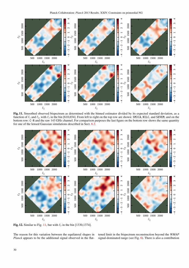
Planck Collaboration: Planck 2013 Results. XXIV. Constraints on primordial NG
500 1000 1500 2000
`1
50
01
00
01
50
02
00
0
` 2
−4−
3−
2−
10
12
34
500 1000 1500 2000
`1
50
01
00
01
50
02
00
0
` 2
−4−
3−
2−
10
12
34
500 1000 1500 2000
`1
50
01
00
01
50
02
00
0
` 2
−4−
3−
2−
10
12
34
500 1000 1500 2000
`1
50
01
00
01
50
02
00
0
` 2
−4−
3−
2−
10
12
34
500 1000 1500 2000
`1
50
01
00
01
50
02
00
0
` 2
−4−
3−
2−
10
12
34
500 1000 1500 2000
`1
50
01
00
01
50
02
00
0
` 2
−4−
3−
2−
10
12
34
Fig. 11. Smoothed observed bispectrum as determined with the binned estimator divided by its expected standard deviation, as afunction of `1 and `2, with `3 in the bin [610,654]. From left to right on the top row are shown: SMICA, NILC, and SEVEM; and on thebottom row: C-R and the raw 143 GHz channel. For comparison purposes the last figure on the bottom row shows the same quantityfor one of the lensed Gaussian simulations described in Sect. 6.2.
500 1000 1500 2000
`1
50
01
00
01
50
02
00
0
` 2
−4−
3−
2−
10
12
34
500 1000 1500 2000
`1
50
01
00
01
50
02
00
0
` 2
−4−
3−
2−
10
12
34
500 1000 1500 2000
`1
50
01
00
01
50
02
00
0
` 2
−4−
3−
2−
10
12
34
500 1000 1500 2000
`1
50
01
00
01
50
02
00
0
` 2
−4−
3−
2−
10
12
34
500 1000 1500 2000
`1
50
01
00
01
50
02
00
0
` 2
−4−
3−
2−
10
12
34
500 1000 1500 2000
`1
50
01
00
01
50
02
00
0
` 2
−4−
3−
2−
10
12
34
Fig. 12. Similar to Fig. 11, but with `3 in the bin [1330,1374].
The reason for this variation between the equilateral shapes inPlanck appears to be the additional signal observed in the flat-
tened limit in the bispectrum reconstruction beyond the WMAPsignal-dominated range (see Fig. 6). There is also a contribution
30

Planck Collaboration: Planck 2013 Results. XXIV. Constraints on primordial NG
from the small correlation difference between equilateral modelsfrom primordial modal and KSW methods. The results for thesemodels for all the SMICA, NILC and SEVEM foreground-separatedmaps are given in Appendix C (Table C.3).
7.3.2. Non-Bunch-Davies vacuum results
We have investigated the non-separable shapes arising from ex-cited initial states (non-Bunch-Davies vacuum models) whichusually peak in the flattened or collinear limit. In particular, wehave searched for the four non-separable bispectra described inEqs. (14) and (15), as well as the original flattened shape BNBD
Φ(Eq. (6.2-3) in Chen et al. 2007b). This entails choosing suit-able cut-offs kc to ensure that the signal is strongly flattened(i.e., distinct from flat in Eq. (13)), while also accurately rep-resented by the modal expansion at both early and late times(Eqs. (54, 55)). For BNBD
Φ, we adopted the same edge truncation
and mild Gaussian filter described in Fergusson et al. (2012),while for BNBD1
Φand BNBD2
Φ, which are described by Eq. (14),
we chose kc = 0.001, and in Eq. (15) we take kc = 0.01. Theshape correlations for most non-Bunch-Davies vacua were good(above 90%), except for the strongly squeezed model with os-cillations of Eq. (14) which was relatively poor (60%). Togetherwith the orthogonal (Eq. (4)), flat (Eq. (13)) and vector (Eq. (19))shapes, these non-Bunch-Davies models explore a broad rangeof flattened models, with a variety of different widths for pickingout signals around the faces of the tetrapyd (see Fig. 1).
The fNL results obtained for the non-Bunch-Davies modelsfrom the different foreground-cleaned map bispectra were con-sistent and the constraints from SMICA (for brevity) are given inTable 11. More comprehensive results from SMICA, NILC andSEVEM can be found in Table C.3 in Appendix C. Both BNBD
Φand
BNBD2Φ
(Eq. (14)) produced raw results above 2σ, in part pickingout the flattened signal observed in the bispectrum reconstruc-tion in Fig. 6. However, these flattened squeezed signals are alsocorrelated with CMB ISW-lensing and so, after subtracting thepredicted ISW bias (as well as the measured point source signal),most NBD fNL results were reduced to 1σ or less (see “CleanfNL” column in Table 11). The exception was the most flattenedmodel BNBD
Φwhich remained higher f NDB
NL = 178 ± 78, i.e., withsignals at 2.0σ, 1.8σ and 2.1σ for SMICA, NILC and SEVEM re-spectively.
We emphasise that this has to be considered just as prelimi-nary study of flattened NG in the Planck data using four exem-plar models. In order to reach a complete statistical assessmentof constraints regarding flattened models in forthcoming anal-yses, we will have to undertake a systematic search for best-fitPlanck NBD models using the parameter freedom available.
7.3.3. Scale-dependent feature and resonant model results
We have investigated whether the Planck bispectrum reconstruc-tions include oscillations expected in feature or resonant models(Eqs. (16, 17)). Although poorly correlated with scale-invariantshapes, the feature and resonant models have (at least) two freeparameters - the period kc and the phase φ - forming a modelspace which must be scanned to determine if there is any sig-nificant correlation (in the absence of any physical motivationfor restricting attention to specific periodicities). We have under-taken an initial survey of these models with the wavelength rangedefined by the native resolution of the present modal estimator(hybrid local polynomials with 600 modes), similar to the featuremodel search in WMAP data in Fergusson et al. (2012). For fea-
ture models of Eq. (16) we can obtain high correlations (above95%) for the predicted CMB bispectrum if we take kc > 0.01,that is, for an effective multipole periodicity `c > 140 featuremodels are accurately represented.
The results of a first survey of feature models in the Planckdata is shown in Table 12 for 0.01 ≤ kc ≤ 0.1 and phasesφ = 0, π/4, π/2, 3π/4 (for φ ≥ π we will identify a correlationwith the opposite sign). Again, there was good consistency be-tween the different foreground-separation methods SMICA, NILCand SEVEM showing that the results are robust to potential resid-ual foreground contamination in the data. For brevity we onlygive SMICA results here, while providing measurements fromother component separation methods in Appendix C. Featuresignals are typically largely uncorrelated with the ISW-lensingor point sources, but nevertheless we subtract these signals andgive results for the cleaned fNL. The Table 12 results show thatthere is a parameter region around 0.01 ≤ kc ≤ 0.025 for whichsignals well in excess of 2σ are possible (we undertook a broadersearch with 0.01 ≤ kc ≤ 0.1 but found only a low signal be-yond k > 0.3). It appears that some feature models are able tomatch the low-` ‘plus-minus’ and other features in the Planckbispectrum reconstruction (see Fig. 6). The best fit model haskc = 0.0185 (`c ≈ 260) and phase φ = 0 with a signal −3σ.As a further validation step of our results, we also re-analysedthe models with > 2.5σ significance using a different modal de-composition, namely an oscillating Fourier basis (nmax = 300)augmented with a local SW mode (the same used for the recon-struction plots in Sect. 7). The results from this basis are shownin Appendix C and they are fully consistent with the polynomialmeasurements presented here. The previous best-fit WMAP fea-ture model, kc = 0.014 (`c ≈ 200) and phase φ = 3π/4, attaineda 2.15σ signal with ` < 500 (Fergusson et al. 2012), but it onlyremains at this level for Planck.
We note however that the apparently high statistical signifi-cance of these results is much lower if we consider this to be ablind survey of feature models, because we are seeking severaluncorrelated models simultaneously. Following what we did forour study of impact of foregrounds in Sect. 8, we considered aset of 200 realistic lensed FFP6 simulations, processed throughthe SMICA pipeline, and including realistic foreground residuals.If we use this accurate MC sample to search for the same gridof 52 feature models as in Table 12, we find a typical maximumsignal of 2.23(±0.56)σ. Searching across all feature models (seebelow) studied here yields an expected maximum 2.37(±0.53)σ(whereas the survey for all 511 models from all paradigms in-vestigated yielded 2.55(±0.52)σ). This means that our best-fitmodel from data has a statistical significance below 1.5σ abovethe maximum signal expectation from simulations, so we con-clude that we have no significant detection of feature modelsfrom Planck data.
Feature models typically have a damping envelope repre-senting the decay of the oscillations as the inflaton returns toits background slow-roll evolution. Indeed, the feature envelopeis a characteristic of the primordial mechanism producing thefluctuations, decaying as k increases for inflation while risingfor contracting models like the ekpyrotic case (Chen 2011). Wehave made an initial survey to determine whether a decayingenvelope improves the significance of any feature models. Theenvelope employed was a Gaussian centred at kc = 0.045 witha falloff ∆k = 0.015, 0.02, 0.025, 0.03, 0.035, 0.04, 0.045 and re-sults for specific parameters are given in Table 13. The best fitmodel remains k = 0.01875 (`c = 265) with phase φ = 0 andthe significance rises to 3.23σ, together with a second modelk = 0.02 (`c = 285) φ = π/4. However the caveats about blind
31

Planck Collaboration: Planck 2013 Results. XXIV. Constraints on primordial NG
Table 11. Constraints on flattened or collinear bispectrum models (and related models) using the SMICA foreground-cleaned Planckmap. These bispectrum shapes, with equation numbers given, are described in detail in the text.
Flattened model (Eq. number) Raw fNL Clean fNL ∆ fNL σ Clean σ
Flat model (13) . . . . . . . . . . . . . . . . . . . 70 37 77 0.9 0.5Non-Bunch-Davies (NBD) . . . . . . . . . . . 178 155 78 2.2 2.0Single-field NBD1 flattened (14) . . . . . . 31 19 13 2.4 1.4Single-field NBD2 squeezed (14) . . . . . . 0.8 0.2 0.4 1.8 0.5Non-canonical NBD3 (15) . . . . . . . . . . . 13 9.6 9.7 1.3 1.0Vector model L = 1 (19) . . . . . . . . . . . . −18 −4.6 47 −0.4 −0.1Vector model L = 2 (19) . . . . . . . . . . . . 2.8 −0.4 2.9 1.0 −0.1
Table 12. Planck bispectrum estimation results for feature models compared to the SMICA foreground-cleaned maps. This pre-liminary survey on a coarse grid in the range 0.01 ≤ kc ≤ 0.025 and 0 ≤ φ < π finds specific models with significance up to99.7%.
fNL ± ∆ fNL (σ)
Wavenumber kc φ = 0 φ = π/4 φ = π/2 φ = 3π/4
0.01000 . . . . . . . . . . −110 ± 159 (−0.7) −98 ± 167 (−0.6) −17 ± 147 (−0.1) 56 ± 142 ( 0.4)0.01125 . . . . . . . . . . 434 ± 170 ( 2.6) 363 ± 185 ( 2.0) 57 ± 183 ( 0.3) −262 ± 168 (−1.6)0.01250 . . . . . . . . . . −70 ± 158 (−0.4) 130 ± 166 ( 0.8) 261 ± 167 ( 1.6) 233 ± 159 ( 1.5)0.01375 . . . . . . . . . . 35 ± 162 ( 0.2) 291 ± 145 ( 2.0) 345 ± 147 ( 2.3) 235 ± 162 ( 1.5)0.01500 . . . . . . . . . . −313 ± 144 (−2.2) −270 ± 137 (−2.0) −95 ± 145 (−0.7) 179 ± 154 ( 1.2)0.01625 . . . . . . . . . . 81 ± 126 ( 0.6) 177 ± 141 ( 1.2) 165 ± 144 ( 1.1) 51 ± 129 ( 0.4)0.01750 . . . . . . . . . . −335 ± 137 (−2.4) −104 ± 128 (−0.8) 181 ± 117 ( 1.5) 366 ± 126 ( 2.9)0.01875 . . . . . . . . . . −348 ± 118 (−3.0) −323 ± 120 (−2.7) −126 ± 119 (−1.1) 137 ± 117 ( 1.2)0.02000 . . . . . . . . . . −155 ± 110 (−1.4) −298 ± 119 (−2.5) −241 ± 113 (−2.1) −44 ± 105 (−0.4)0.02125 . . . . . . . . . . −43 ± 96 (−0.4) −186 ± 107 (−1.7) −229 ± 115 (−2.0) −125 ± 104 (−1.2)0.02250 . . . . . . . . . . 22 ± 95 ( 0.2) −115 ± 92 (−1.2) −194 ± 105 (−1.8) −148 ± 107 (−1.4)0.02375 . . . . . . . . . . 70 ± 100 ( 0.7) −56 ± 94 (−0.6) −159 ± 93 (−1.7) −164 ± 101 (−1.6)0.02500 . . . . . . . . . . 106 ± 93 ( 1.1) 6 ± 97 ( 0.1) −103 ± 98 (−1.1) −153 ± 94 (−1.6)
Table 13. Feature model results with an envelope decay function of width ∆k. Results are only presented for feature models withbetter than 95% CL result on the full domain (see Table 12).
fNL ± ∆ fNL (σ)
Wavenumber kc; phase ∆k = 0.015 ∆k = 0.03 ∆k = 0.045 Full
0.01125; φ = 0 . . . . . 765 ± 275 ( 2.8) 703 ± 241 ( 2.9) 648 ± 218 ( 3.0) 434 ± 170 ( 2.6)0.01750; φ = 0 . . . . . −661 ± 234 (−2.8) −494 ± 192 (−2.6) −425 ± 171 (−2.5) −335 ± 137 (−2.4)0.01750; φ = 3π/4 . . 399 ± 207 ( 1.9) 438 ± 183 ( 2.4) 442 ± 165 ( 2.7) 366 ± 126 ( 2.9)0.01875; φ = 0 . . . . . −562 ± 211 (−2.7) −559 ± 180 (−3.1) −515 ± 159 (−3.2) −348 ± 118 (−3.0)0.01875; φ = π/4 . . . −646 ± 240 (−2.7) −525 ± 189 (−2.8) −468 ± 164 (−2.9) −323 ± 120 (−2.7)0.02000; φ = π/4 . . . −665 ± 229 (−2.9) −593 ± 185 (−3.2) −500 ± 160 (−3.1) −298 ± 119 (−2.5)
survey statistics previously noted also do not allow a claim ofany detection in this case. A plot of the best-fit feature modelwith a decay envelope is shown in Fig. 13, for which the mainfeatures should be compared with those in Fig. 7. Non-Gaussianbispectrum signals from feature models typically produce coun-terparts in the power spectrum as will be described in Sect. 9. Animproved statistical interpretation of the results presented in thisSection will be possible when this additional investigation willbe completed.
We have also undertaken a survey of resonant models andthe non-Bunch-Davies resonant models (or enfolded resonancemodels). With the modal estimator, we can achieve high ac-curacy for the predicted bispectrum for kc > 0.001 (note thatthis has a different logarithmic dependence to feature modelsand a varying effective `c). For the resonance model shape ofEq. (18), we have not undertaken an extensive survey, except
selecting a likely range for a high signal with periodicity com-parable to the feature model, that is, with 0.25 < kc < 0.5and phases φ = 0, π/4, π/2, 3π/4, π. However, no signif-icant signal was found (all below 1σ), as can be verified inTable C.1 in Appendix C. For the enfolded resonance modelshape of Eq. (18) , we have undertaken a preliminary search inthe range 4 < kc < 12 with the same phases. Again, no signifi-cant signal emerges from the Planck data, as shown in Table C.2in Appendix C.
7.3.4. Directional dependence motivated by gauge fields
We have investigated whether there is significant NG frombispectrum shapes with non-trivial directional dependence(Eq. (19)), which are motivated by inflationary models with vec-
32

Planck Collaboration: Planck 2013 Results. XXIV. Constraints on primordial NG
Fig. 13. CMB bispectrum shown for the best-fit feature modelwith an envelope with parameters k = 0.01875, phase φ = 0 and∆k = 0.045 (see Table 13). Compare with the Planck bispectrumreconstruction, Fig. 7.
tor fields. Using the primordial modal estimator we obtained agood correlation with the L = 1 flattened-type model, but thesqueezed L = 2 model produced a relatively poor correlationof only 60%, given the complexity of the dominant squeezedlimit. Preliminary constraints on these models are given in theTable 11, showing no evidence of a significant signal.
7.3.5. Warm inflation
Warm inflation produces a related shape with a sign changein the squeezed limit. This also had a poor correlation, untilsmoothing (WarmS) was applied as described in Fergusson et al.(2012). The resulting bispectrum shows no evidence for signifi-cant correlation with Planck data (SMICA),
f WarmSNL = 4 ± 33 . (87)
The full list of constraints for SMICA, NILC and SEVEM modelscan be found for warm inflation and vector models in Table C.3in Appendix C.
7.3.6. Quasi-single-field inflation
Finally, quasi-single-field inflation has been analysed constrain-ing the bispectrum shape of Q (Eq. (12)), that depends on twoparameters, ν and f QSI
NL . In order to constrain this model we havecalculated modal coefficients for 0 ≤ ν ≤ 1.5 in steps of 0.01(so 151 models in total). These were then applied to the dataand the one with the greatest significance was selected. Resultsare shown in Fig. 26. The maximum signal occurred at ν = 1.5,f QSINL = 4.79 (0.31σ). To obtain error curves we performed a
full likelihood using 2 billion simulations following the methoddescribed in Sefusatti et al. (2012). Such a large number of sim-ulations was possible as they were generated from the modal β-covariance matrix which is calculated once from the 200 Planckrealistic CMB simulations, rather than repeatedly from the CMBsimulations themselves. The procedure is to take the 151 × 151correlation matrix for the models (this is just the normalized dot
0.
00.
20.
40.
60.
81.
0
0 500 1000 1500 2000 2500 3000
W
ℓ
WM
Fig. 14. The Wiener filter WM used to constrain f localNL with MFs.
Table 14. Validation tests with MFs: results for f localNL obtained
using the filter WM, for `max = 2000 and Nside = 2048.
Setup f localNL (MFs)
Gaussian ideal 0.2 ± 10.7Realistic noise, f local
NL = 12 12 ± 13Mask ( fsky = 0.73), realistic noise f local
NL = 12 12 ± 18
product of the modal coefficients). This is then diagonalised us-ing PCA, after which only the first 5 eigenvalues are kept as theremaining eigenvalues are < 10−10. The β-covariance matrix isprojected into the same sub-basis where it is also diagonalisedvia PCA into 5 orthonormal modes, with the two leading modesclosely correlated with local and equilateral. The procedure bywhich to produce a simulation is to generate five Gaussian ran-dom numbers and add the mean values obtained from the Planckdata, rotating them to the sub-basis where we determine the νwith the greatest significance. The result is then projected backto the original space to determine the related fNL. The two billionresults from this MC analysis are then converted into confidencecurves plotted in Fig. 26. The curve shows that there is no pre-ferred value for ν with all values allowed at 3σ. This reflects theresults obtained from data previously, where we found the leastpreferred value of ν = 0.86 had only a marginally lower signif-icance of 0.28σ (Sefusatti et al. 2012). Of course, these conclu-sions are directly related to the null results for both local andequilateral templates.
7.4. Constraints on local non-Gaussianity with MinkowskiFunctionals
In this Subsection, we present constraints on local NG ob-tained with Minkowski Functionals (MFs). MFs describe themorphological properties of the CMB field and can be used asgeneric estimators of NG (Komatsu et al. 2003; Eriksen et al.2004; De Troia et al. 2007; Hikage et al. 2008; Curto et al. 2008;Natoli et al. 2010; Hikage & Matsubara 2012; Modest et al.2013). As they are sensitive to every order of NG, theycan be used to constrain different bispectrum and trispectrumshapes (Hikage et al. 2006, 2008; Hikage & Matsubara 2012).They are therefore complementary to, and a useful valida-tion of, optimal estimators. Their precise definition and ana-lytic formulations are presented in Planck Collaboration XXIII
33

Planck Collaboration: Planck 2013 Results. XXIV. Constraints on primordial NG
−0.0
020.
000
0.00
2
−2 0 2
SMICA
(a)
−0.0
020.
000
0.00
2
−2 0 2
−0
.005
0.00
00.
005
−2 0 2
SMICA
(b)
−0
.005
0.00
00.
005
−2 0 2
−0
.04
0.00
0.04
−2 0 2
SMICA
(c)
−0
.04
0.00
0.04
−2 0 2
−0
.04
0.00
−2 0 2
SMICA
(d)
−0
.04
0.00
−2 0 2νννν
νννν
(v0
−vG 0
)/vG
,max
0(v
0−
vG 0
)/vG
,max
0
(v1
−vG 1
)/vG
,max
1(v
1−
vG 1
)/vG
,max
1
(v2
−vG 2
)/vG
,max
2(v
2−
vG 2
)/vG
,max
2
(v3
−vG 3
)/vG
,max
3(v
3−
vG 3
)/vG
,max
3
fsky = 0.73, WMfsky = 0.73, WM
fsky = 0.73, WMfsky = 0.73, WM
f localNL = 50f local
NL = 50
f localNL = 50f local
NL = 50
Fig. 15. The MFs curves for SMICA at Nside = 1024 and `max = 2000, for the four functionals vk: (a) Area, (b) Perimeter, (c)Genus, and (d) Ncluster. The curves are the difference of each normalized MF, measured from the data, to the average from GaussianPlanck realistic simulations (not lensed). The difference curves are normalized by the maximum of the Gaussian curve. To comparethe curves to the presence of primordial NG, the average difference curves for non-Gaussian simulations with f local
NL = 50 is alsorepresented (100 simulations).
Table 15. Estimates of f localNL obtained with MFs on Planck data. Foreground and secondary effects are evaluated in terms of f local
NL .Results are for SMICA at Nside = 1024 and `max = 2000.
Map f localNL Source Corresponding ∆ f local
NL
Raw map . . . . . . . . . 19.1 ± 19.3Lensing subtracted . . 8.5 ± 20.5 Lensing +10.6Lensing+PS subtracted 7.7 ± 20.3 Point sources +0.8Lensing+CIB subtracted 7.5 ± 20.5 CIB +1.0Lensing+SZ subtracted 6.0 ± 20.4 SZ +2.5All subtracted . . . . . . 4.2 ± 20.5 All +14.9
(2013). The MF technique is also used in the companion paperPlanck Collaboration XXV (2013).
We review here the properties of MFs, as a complementarytool to poly-spectrum based estimators.
First, they are defined in real space, which makes MFs ro-bust to masking effects and no linear term is needed to takeinto account the anisotropy of the data model. Second, as MFsare sensitive to every non-Gaussian feature in the maps, theycan be a useful probe of every potential bias in the bispectrummeasurement, in particular the different astrophysical contami-nations (foregrounds and secondaries).
There is a limitation to MF studies: they can be expressed interms of weighted sums of the bispectrum (and trispectrum) inharmonic space (Matsubara 2010), hence the angle-dependence
of the bispectrum is partially lost. This makes MFs subopti-mal in two ways: increasing error bars for constraints on spe-cific shapes and reducing the distinguishability of different bis-pectrum shapes. This lack of specificity can introduce biases,as MFs will partially confuse primordial and non-primordialsources of NG and can introduce degeneracies between differ-ent primordial shapes. Constraints on orthogonal and equilateralshapes are quite degenerate with MFs, we therefore chose here tofocus on the local bispectrum shape. We also leave trispectrumanalyses for future studies.
An attractive feature of MFs is their linearity for weakNG ( fNL) and weak signals (such as point sources, andGalactic residuals after masking and component separation)
34

Planck Collaboration: Planck 2013 Results. XXIV. Constraints on primordial NG
(Ducout et al. 2013). This property can be used to estimate dif-ferent known non-primordial contributions.
7.4.1. Method
We constrain f localNL using the optimized procedure described in
Ducout et al. (2013). To obtain constraints on f localNL , we apply a
specific Wiener filter on the map (WM), shown in Fig. 14. We donot use here the filter designed to enhance the information fromthe gradients of the map (WD1 =
√`(` + 1)WM), because this
filter is very sensitive to small-scale effects and may be biasedby foreground residuals.
We use maps at HEALPix resolution Nside =1024 (Gorski et al. 2005) and `max = 2000. Our resultsare based on the four normalized14 functionals vk (k = 0, 3)(respectively Area, Perimeter, Genus and Ncluster), computed onnth = 26 thresholds ν, between νmin = −3.5 and νmax = +3.5 inunits of the standard deviation of the map.
We combine all functionals into one vector y (of size n =104). We then analyse this vector in a Bayesian way to obtaina posterior for the f local
NL , and hence an estimate of this parame-ter. The principle is to compare the vector measured on the datay to the ones measured on non-Gaussian simulations with thesame systematic effects (realistic noise, effective beam) and dataprocessing (Wiener filtering) as the data, y( f local
NL ). Modelling theMFs as multivariate Gaussians we obtain the posterior distribu-tion for f local
NL with a χ2 test :
P( f localNL | y) ∝ exp
−χ2(y, f localNL )
2
(88)
with
χ2(y, f localNL ) ≡
[y − y( f local
NL )]T
C−1[y − y( f local
NL )], (89)
Since NG is weak, the covariance matrix C is computed with104 Gaussian simulations, again reproducing effective beam, re-alistic noise and filtering of the data. The dependence of the MFson f local
NL , y( f localNL ), is obtained as an average of ymeasured on 100
simulations. The simulations used here are based on the WMAP-7 best-fit power spectrum (Komatsu et al. 2011), using the pro-cedure described in Elsner & Wandelt (2009).
7.4.2. Validation tests
We report here validation of the MFs estimator on f localNL in
thoroughly realistic Planck simulations. This validation subsec-tion is analogous to Sect. 6.1 concerning bispectrum-based es-timators. The same tests (ideal Gaussian maps, full-sky non-Gaussian maps with noise and non-Gaussian maps with noiseand mask) are performed, but different non-Gaussian simula-tions are used. Non-Gaussian CMB simulations as processed inFergusson et al. (2010a) only guarantee the correctness of the 3-point correlations. Since the MFs are sensitive to higher-ordern-point functions, they were validated with physical simulations(Elsner & Wandelt 2009).
The first test consists of 100 simulations of a full-skyGaussian CMB, with a Gaussian beam with FWHM of 5 arcminand without any noise, cut off at `max = 2000, with Nside = 2048.
14 Raw MFs Vk depend on the Gaussian part of fields through a nor-malization factor Ak that is a function only of the power spectrum shape.We therefore normalize functionals vk = Vk/Ak to focus on NG; seePlanck Collaboration XXIII (2013) and references therein.
Here validation tests were made at Nside = 2048, but results (es-timate and error bars) remain the same at Nside = 1024 as wekeep the same `max. The second test includes non-Gaussian sim-ulations with f local
NL = 12 and realistic coloured and anisotropicnoise, processed through the Planck simulation pipeline and thecomponent-separation method SMICA. Finally, in the third testwe add the union mask U73 to the previous simulations, mask-ing both the Galaxy and the brightest point sources, and leaving73% of the sky unmasked. Only the inpainting of the smallestholes in the point sources part of the mask was performed. Forthese three tests, the results are presented in Table 14. We givehere the average estimate and error bar obtained on the 100 simu-lations, when we use the four functionals. The results show thatthe MF estimator is unbiased, robust, and a competitive alter-native to bispectrum-based estimators. Moreover a map-by-mapcomparison of the results obtained on f local
NL with KSW and MFsestimators showed a fair agreement between the two methods.
7.4.3. Results
For our analysis we considered a foreground-cleaned mapobtained with the component separation method SMICA atNside = 1024 and `max = 2000. As for the previous results in thisSection, we used the union mask U73, which leaves fsky = 73%of the sky after masking Galaxy and point sources. To take intoaccount some instrumental effects (asymmetry of beams, com-ponent separation processing) and known non-Gaussian contri-butions (lensing), we used realistic unlensed and lensed simula-tions (103) of Planck data (FFP6 simulations, see Appendix A).First, MFs were applied to the unlensed simulations and the re-sulting curves served to calibrate the estimator, as the Gaussianpart of the NG curves y( f local
NL )15. This estimate is referred to asthe “raw map”. Secondly, MFs were applied to the lensed sim-ulations, and the same procedure was applied, the result beingreferred as “lensing-subtracted”. We summarize the procedurein the following equation:
y( f localNL ) = yG
Planck simulations, lensed + ∆yNGfNL, NG simulations (90)
Here we assume that the MF respond linearly to lensing at firstorder and that primordial NG and lensing contributions are there-fore additive.
Additionally, we tried to characterize other non-primordialcontributions that one could expect in masked SMICA-cleanedmaps covering 73% of the sky. To this end, we used simula-tions of extragalactic foregrounds and secondary anisotropies:uncorrelated (Poissonian) point sources; clustered CIB; andSZ clusters. These component simulations reproduce accuratelythe whole Planck data processing pipeline (beam asymme-try, component separation method). Using the linearity of MFs(Ducout et al. 2013), we could introduce these effects as a simpleadditive bias on the curves following
y = yFGsubtracted + ∆yPS + ∆yCIB + ∆ySZ (91)
where ∆yPS,... is the average bias measured on 100 simulations.Note that the SZ simulation does not take into account the SZ-lensing correlation, which is expected to be negligible given theerror bars.
Results are summarized in Table 15 and MFs curves areshown in Fig. 15, without including the lensing subtraction
15 The overall effect of data processing on the f localNL constraint from
MFs was evaluated as f localNL (process.) ∼ 3.
35
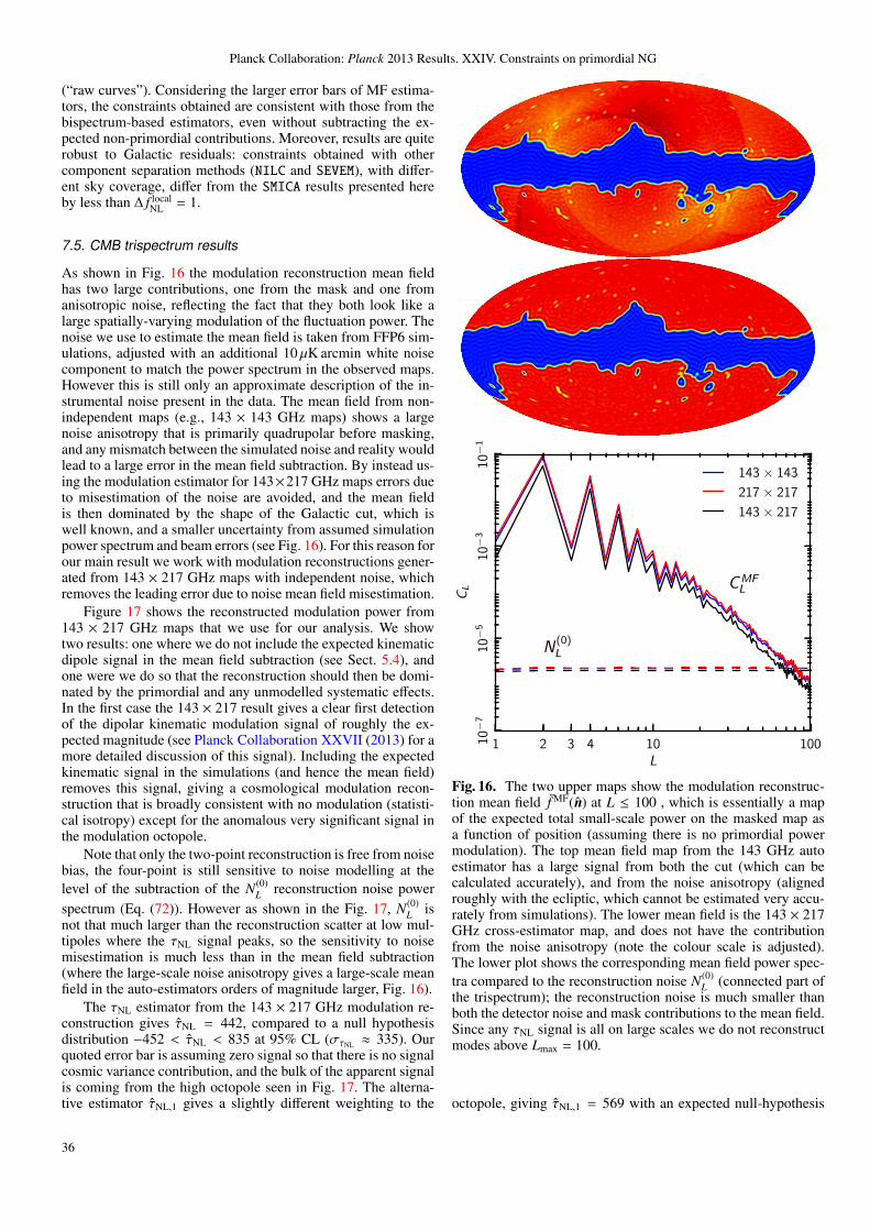
Planck Collaboration: Planck 2013 Results. XXIV. Constraints on primordial NG
(“raw curves”). Considering the larger error bars of MF estima-tors, the constraints obtained are consistent with those from thebispectrum-based estimators, even without subtracting the ex-pected non-primordial contributions. Moreover, results are quiterobust to Galactic residuals: constraints obtained with othercomponent separation methods (NILC and SEVEM), with differ-ent sky coverage, differ from the SMICA results presented hereby less than ∆ f local
NL = 1.
7.5. CMB trispectrum results
As shown in Fig. 16 the modulation reconstruction mean fieldhas two large contributions, one from the mask and one fromanisotropic noise, reflecting the fact that they both look like alarge spatially-varying modulation of the fluctuation power. Thenoise we use to estimate the mean field is taken from FFP6 sim-ulations, adjusted with an additional 10 µK arcmin white noisecomponent to match the power spectrum in the observed maps.However this is still only an approximate description of the in-strumental noise present in the data. The mean field from non-independent maps (e.g., 143 × 143 GHz maps) shows a largenoise anisotropy that is primarily quadrupolar before masking,and any mismatch between the simulated noise and reality wouldlead to a large error in the mean field subtraction. By instead us-ing the modulation estimator for 143×217 GHz maps errors dueto misestimation of the noise are avoided, and the mean fieldis then dominated by the shape of the Galactic cut, which iswell known, and a smaller uncertainty from assumed simulationpower spectrum and beam errors (see Fig. 16). For this reason forour main result we work with modulation reconstructions gener-ated from 143 × 217 GHz maps with independent noise, whichremoves the leading error due to noise mean field misestimation.
Figure 17 shows the reconstructed modulation power from143 × 217 GHz maps that we use for our analysis. We showtwo results: one where we do not include the expected kinematicdipole signal in the mean field subtraction (see Sect. 5.4), andone were we do so that the reconstruction should then be domi-nated by the primordial and any unmodelled systematic effects.In the first case the 143 × 217 result gives a clear first detectionof the dipolar kinematic modulation signal of roughly the ex-pected magnitude (see Planck Collaboration XXVII (2013) for amore detailed discussion of this signal). Including the expectedkinematic signal in the simulations (and hence the mean field)removes this signal, giving a cosmological modulation recon-struction that is broadly consistent with no modulation (statisti-cal isotropy) except for the anomalous very significant signal inthe modulation octopole.
Note that only the two-point reconstruction is free from noisebias, the four-point is still sensitive to noise modelling at thelevel of the subtraction of the N(0)
L reconstruction noise powerspectrum (Eq. (72)). However as shown in the Fig. 17, N(0)
L isnot that much larger than the reconstruction scatter at low mul-tipoles where the τNL signal peaks, so the sensitivity to noisemisestimation is much less than in the mean field subtraction(where the large-scale noise anisotropy gives a large-scale meanfield in the auto-estimators orders of magnitude larger, Fig. 16).
The τNL estimator from the 143 × 217 GHz modulation re-construction gives τNL = 442, compared to a null hypothesisdistribution −452 < τNL < 835 at 95% CL (στNL ≈ 335). Ourquoted error bar is assuming zero signal so that there is no signalcosmic variance contribution, and the bulk of the apparent signalis coming from the high octopole seen in Fig. 17. The alterna-tive estimator τNL,1 gives a slightly different weighting to the
1 2 3 4 10 100L
10�
710�
510�
310�
1
CL CMF
L
N(0)L
143⇥ 143
217⇥ 217
143⇥ 217
Fig. 16. The two upper maps show the modulation reconstruc-tion mean field f MF(n) at L ≤ 100 , which is essentially a mapof the expected total small-scale power on the masked map asa function of position (assuming there is no primordial powermodulation). The top mean field map from the 143 GHz autoestimator has a large signal from both the cut (which can becalculated accurately), and from the noise anisotropy (alignedroughly with the ecliptic, which cannot be estimated very accu-rately from simulations). The lower mean field is the 143 × 217GHz cross-estimator map, and does not have the contributionfrom the noise anisotropy (note the colour scale is adjusted).The lower plot shows the corresponding mean field power spec-tra compared to the reconstruction noise N(0)
L (connected part ofthe trispectrum); the reconstruction noise is much smaller thanboth the detector noise and mask contributions to the mean field.Since any τNL signal is all on large scales we do not reconstructmodes above Lmax = 100.
octopole, giving τNL,1 = 569 with an expected null-hypothesis
36

Planck Collaboration: Planck 2013 Results. XXIV. Constraints on primordial NG
1 2 3 4 10 100L
�0.
50.
00.
51.
01.
52.
02.
5
CL
⇥10�5
143⇥ 217 N(0)
Cf
Cf (kinematic removed)
Kinematic dipole
⌧NL = 1000
Fig. 17. Power spectrum of the power modulation reconstructedfrom 143 × 217 GHz maps. Shading shows the 68%, 95% and99% CL intervals from simulations with no modulation or kine-matic signal. The dashed lines are when the mean field simula-tions include no kinematic effects, showing a clear detection of amodulation dipole. The blue points show the expected kinematicmodulation dipole signal from simulations, along with 1σ errorbars (only first four points shown for clarity). The solid line sub-tracts the dipolar kinematic signal in the mean fields from sim-ulations including the expected signal, and represents out bestestimate of the non-kinematic signal (note this is not just a sub-traction of the power spectra since the mean field takes out thefixed dipole anisotropy in real space before calculating the re-maining modulation power). The dotted line shows the expectedsignal for τNL = 1000.
στNL ≈ 332. The surprisingly large difference between the es-timators can be explained as due to the large octopole signal,which has τNL(L = 3) ≈ 6000. However the shape of the totalsignal would not be expected from a genuine τNL signal, sinceas shown in Fig. 17 on average the latter is expected to fall offapproximately proportional to 1/L2 (i.e., a large primordial τNLwould be expected in most realisations to give large dipole andquadrupole signals that we do not see). If we estimate τNL usingLmax = 2 we obtain τNL = 165 with only a slightly larger null-hypothesis error στNL = 349, where in this case τNL,1 = 172.
Note that the distribution of τNL is quite skewed becausethe signal is dominated by the very-low multipole modulationpower spectra which have skewed χ2-like distributions due tothe large cosmic variance there (see Fig. 18; Hanson & Lewis2009; Smith & Kamionkowski 2012). The reconstruction noiseacts like nearly-uncorrelated Gaussian white noise, so each ofthe C f
L comes from a sum of squares of ∼ 2L + 1 modulation re-construction modes; the shape of the τNL distribution is consis-tent with what would come from calculating a weighted sum ofχ2-distributed random variables. If we assume that any primor-dial modulation modes giving rise to a physical τNL signal arealso Gaussian, for any given physical τNL the τNL(L) estimatorswould also have χ2 distributions. This allows us to evaluate theposterior distribution of τNL given the observed τNL, in exactlythe same way that one can do for the CMB temperature power
�500 0 500 1000 1500 2000
⌧NL
0.00
020.
0006
0.00
100.
0014
Bin
ned
prob
abili
ty
Fig. 18. Distribution of τNL estimators from Gaussian simula-tions (Lmax = 10) compared to data estimates (vertical lines).The distribution is rather skewed because the main contributionsare from L <
∼ 4 where the modulation power spectra have skewedχ2 distributions with low degrees of freedom. The red line showsthe predicted distribution for a weighted sum of τNL(L) estima-tors assuming the reconstructed modulation modes are Gaussianwith 2L + 1 modes measured per L, which fits the full simula-tions well. The black vertical lines show the data estimates fromLmax = 10, and should be compared to the green which haveLmax = 2 and hence are insensitive to the anomalous octopolesignal. The dashed lines are τNL,1, the slightly more optimal vari-ant of the estimator.
spectrum. For each L the posterior distribution P(τNL(L)|τNL(L))on the full sky would have an inverse-gamma distribution. Wefollow Hamimeche & Lewis (2008) by generalizing this to a cut-sky approximation for a range of multipoles:
− 2 ln P({τNL(L)}|{τNL(L)}) ≈∑LL′
[g(x(L))N(0)
τNL(L)
] [M−1
]LL′
[N(0)τNL
(L′)g(x(L′))]
(92)
where MLL′ is the covariance of the estimators calculated fromnull hypothesis simulations, N(0)
τNL (L) = kLN(0)L /Cζ∗
L is the estima-tor reconstruction noise,
x(L) ≡τNL(L) + N(0)
τNL (L)
τNL(L) + N(0)τNL (L)
, (93)
andg(x) ≡ sign(x − 1)
√2(x − ln(x) − 1). (94)
For uncorrelated χ2-distributed estimators this distribution re-duces to the exact distribution, a product of inverse-gamma dis-tributions. This approximation to the posterior can be used toevaluate the probability of any scale dependent τNL(L), and doesnot rely on compression into a single τNL estimator; it can there-fore fully account for the observed distribution of modulationpower between L. Here we focus on the main case of interestwhere τNL(L) is nearly-scale-invariant so that for all L we haveτNL(L) = τNL.
The resulting posterior distributions of τNL are shown inFig. 19 for a range of Lmax. These are strongly skewed, in the
37

Planck Collaboration: Planck 2013 Results. XXIV. Constraints on primordial NG
0 1000 2000 3000 4000 5000 6000⌧NL
0.00
000.
0002
0.00
040.
0006
0.00
08
P(⌧
NL)
Lmax = 2
Lmax = 3
Lmax = 6
Lmax = 10
Lmax = 20
Lmax = 50
Fig. 19. Approximate posterior distributions P(τNL|τNL(L)) for arange of Lmax. The distributions have broad tails to high valuesbecause of the small number of large-scale modulation modesthat are measured, and hence large cosmic variance. For Lmax ≥
3 the distributions are pulled away from zero by the significantoctopole modulation signal observed, and are gradually moveback towards zero as we include more modulation modes thatare inconsistent with large τNL values. As shown in Fig. 20 theoctopole has significant frequency dependence and is thereforeunlikely to be physical.
same way as the posterior from the low quadrupole in the CMBtemperature data. The high octopole is pulling the distributionsup to higher τNL values, but increasing Lmax can reduce the high-L tail because very large τNL values are inconsistent with the lowmodulation power seen at L , 3. With Lmax = 2 the posteriorpeaks near zero, but the distribution is then very broad becausethere are only about 8 modes, which therefore have large cosmicvariance. For Lmax = 50 we find τNL < 2800 at 95% CL, whichwe take as our upper limit.
Figure 20 shows the modulation reconstructions for the 143GHz and 217 GHz maps separately compared to the cross esti-mator. The picture is complicated here by the large signals fromnoise misestimation seen in the 143 × 143 and 217 × 217 esti-mators, however the fact that the octopole in 143 × 143 is lowerthan in the cross-estimator indicates that the octopole signal isvery unlikely to be mainly physical. Our measured τNL limit inpractice represents a strong upper limit on the level of primor-dial τNL that could be present, since unmodelled varying small-scale foreground or non-constant gain/calibration would alsoonly serve to increase the measured estimate compared to pri-mordial on average. The octopole signal does vary slightly withGalactic mask, though at present we cannot clearly isolate itsorigin. If more extensive analysis (for example using cross-mapestimators at the same frequency) can identify a non-physicalorigin and remove it, the quoted upper limit on τNL would be-come significantly tighter. For a more extensive discussion ofpossible foreground and systematic effect issues that can af-fect 4-point estimators see Planck Collaboration XXVII (2013);Planck Collaboration XVII (2013).
We have focussed on nearly scale invariant modulationshere. As discussed in Planck Collaboration XXIII (2013) there
0.0
0.5
1.0
1.5
CL
⇥10�5
143⇥ 143N
(0)L
C fL (kinematic removed)
⌧NL = 1000
0.0
0.5
1.0
1.5
CL
143⇥ 217
1 2 3 4 10 100L
0.0
0.5
1.0
1.5
CL
217⇥ 217
Fig. 20. Comparison of the un-normalized modulation powerC f
L with various combinations of frequencies. The middle plotshows the results used for our main τNL result, since it removesthe significant largely-quadrupolar signal from anisotropic noisemisestimation seen in the two other plots. The noticeable differ-ence in the odd octopole signal between channels indicates thatthe residual signal in 143 × 217 GHz is unlikely to be physical,but we cannot currently identify its origin.
are some potentially interesting “anomalies” in the distributionof power in the Planck data, especially the hemispherical powerasymmetry at `max ≤ 600. If these power asymmetries are phys-ical rather than statistical flukes, they must be strongly scale-dependent, and would correspond to a scale-dependent τNL-like
38

Planck Collaboration: Planck 2013 Results. XXIV. Constraints on primordial NG
Fig. 21. The dependence of the dipole modulation amplitude asa function of `max. Upper panel: the amplitude | f | of the dipole ofthe reconstructed power modulation from 143 × 217 GHz mapswith the kinematic dipole subtracted; the dashed line shows thatthe observed signal decreases with `max in the same way asthe r.m.s. value expected from simulations. Lower panel: corre-sponding confidence values for the observed dipole of the mod-ulation power spectrum C f assuming it followed a chi-squareddistribution; this shows the anomalous-looking results for `max ∼
60 and `max ∼ 600 consistent with Planck Collaboration XXVII(2013), but that on smaller scales the observed signal is consis-tent with isotropy as expected from the scale-invariant C f (L = 1)constraint using `max = 2000 shown in Fig. 17.
trispectrum. As we have shown here the dipole power asym-metry does not persist to small scales, except for the signalaligned with the CMB dipole expected from kinematic effects:from our analysis using `max = 2000 we find a primordialτNL(L = 1) consistent with Gaussian simulations, correspond-ing to a dipole modulation amplitude | f | ∼ 0.2%. To be con-sistent with a ∼ 7% modulation at `max ∼ 60 and ∼ 1% mod-ulation at `max 600, as seen in the lower-` anisotropies of bothWMAP and Planck the primordial trispectrum would have tobe strongly scale-dependent on small-scale modes, so that largersmall-scale modes are modulated more than the smallest ones(rather than just τNL = τNL(L)). Fig. 21 shows how the alloweddipole modulation amplitude drops as `max increases (similar toFig. 3 of Hanson & Lewis (2009) for WMAP, but now extend-ing to the higher `max available from Planck). This result is con-sistent with Planck Collaboration XXIII (2013), where differentestimators and analysis cuts also find no evidence of primordialdipole-like power asymmetry on small scales, but confirm thelarge-scale distribution of power seen with WMAP and also amarginally-significant smaller-amplitude ( f ∼ 1%) dipole-likemodulation at `max ∼ 600.
8. Validation of Planck results
Here we perform a set of tests to check the robustness and sta-bility of our fNL measurements. As these are validation testsof Planck results, and not internal comparisons of bispectrumpipelines (already shown to be in tight agreement in Sect. 6 and7) we will not employ all the bispectrum estimators on each test.In general we choose to use two estimators on each test, in orderto have a cross-check of the outcomes without excessive redun-dancy.
8.1. Dependence on maximum multipole number
The dependence on the maximum multipole number `max of theSMICA results (assuming independent shapes) is shown in Fig. 22(for the binned estimator) and Table 16 (for both the KSW andbinned estimators). Testing the `max dependence is easiest for thebinned estimator, where one can simply omit the highest binsin the final sum when computing fNL. It is clear that we havereached convergence both for the values of fNL and for their errorbars at `max = 2500, with the possible exception of the error barsof the diffuse point-source bispectrum. The diffuse point-sourcebispectrum template is dominated by equilateral configurationsat high `. Moreover, for all the shapes except point sources, re-sults at `max = 2000 are very close to those at `max = 2500,taking into account the size of the error bars.
It is very interesting to see that at `max ∼ 500 we find a localfNL result in very good agreement with the WMAP-9 value of39.8±19.9 (Bennett et al. 2012) (or 37.2±19.9 after ISW-lensingbias subtraction). At these low `max values we also find negativevalues for orthogonal fNL, although not as large or significant asthe WMAP-9 value (which is −245 ± 100). One can clearly seethe importance of the higher resolution of Planck both for thevalues of the different fNL parameters and for their error bars.
It is also clear that the higher resolution of Planck is abso-lutely crucial for the ISW-lensing bispectrum; this is simply un-detectable at WMAP resolution. On the other hand, the high sen-sitivity of Planck measurements also exposes us to a larger num-ber of potentially spurious effects. For example we see that thebispectrum of point sources is also detected at high significanceby Planck at `max ≥ 2000, while remaining undetectable at lowerresolutions. The presence of this bipectrum in the data could inprinciple contaminate our primordial fNL measurements. For thisreason, the presence of a large point source signal has been ac-counted for in previous Sections by always including the Poissonbispectrum in a joint fit with primordial shapes. Fortunately, itturns out that the very low correlation between the primordialtemplates and the Poisson one makes the latter a negligible con-taminant for fNL, even when the residual point source amplitudeis large.
8.2. Dependence on mask and consistency betweenfrequency channels
To test the dependence on the mask, we have analysed theSMICA maps applying four different masks. Firstly the unionmask U73 used for the final results in Sect. 7, which leaves73% of the sky unmasked. Secondly we used the confidencemask CS-SMICA89 of the SMICA technique, which leaves 89%of the sky. Next, a bigger mask constructed by multiplying theunion mask U73 with the Planck Galactic mask CG60, leadingto a mask that leaves 56% of the sky. And finally a very largemask, leaving only 32% of the sky, which is the union of themask CL31 - used for power spectrum estimation on the raw
39

Planck Collaboration: Planck 2013 Results. XXIV. Constraints on primordial NG
500 1000 1500 2000 2500
`max
−4
0−
20
02
04
0
flo
cal
NL
500 1000 1500 2000 2500
`max
−4
00−
20
00
20
04
00
feq
uil
NL
500 1000 1500 2000 2500
`max
−2
00−
10
00
10
02
00
for
tho
NL
500 1000 1500 2000 2500
`max
−1
00
10
20
30
Poi
nt
sou
rce
bis
p.
amp
l.×
102
9..
.
500 1000 1500 2000 2500
`max
−2−
10
12
34
fle
ns
NL
500 1000 1500 2000 2500
`max
−4
0−
20
02
04
06
0
flo
cal
NL
Fig. 22. Evolution of the fNL parameters (solid blue line with data points) and their uncertainties (dashed lines) for the five bispectrumtemplates as a function of the maximum multipole number `max used in the analysis. From left to right and top to bottom the figuresshow respectively local, equilateral, orthogonal, diffuse point sources (all four with the ISW-lensing bias subtracted), ISW-lensingand local again (the last two without subtracting the ISW-lensing bias). To show better the evolution of the uncertainties, they arealso plotted around the final value of fNL (solid green lines without data points). The results are for SMICA, assume all shapes to beindependent, and have been determined with the binned bispectrum estimator.
Table 16. Results for fNL (assumed independent, without any correction for the ISW-lensing bias) of the SMICA cleaned map usingdifferent values of `max, for the KSW and binned estimators.
fNL
Shape `max = 500 `max = 1000 `max = 1500 `max = 2000 `max = 2500
KSWLocal . . . . . . . . . 38 ± 18 6.4 ± 9.7 6.9 ± 6.2 9.1 ± 5.8 9.8 ± 5.8Equilateral . . . . . −119 ± 121 −45 ± 88 −41 ± 75 −40 ± 75 −37 ± 75Orthogonal . . . . . −163 ± 109 −89 ± 52 −57 ± 45 −45 ± 40 −46 ± 39Diff.ps /10−29 . . . (−1.5 ± 1.3)×104 (−7.9 ± 3.1)×102 −39 ± 18 10.0 ± 3.1 7.7 ± 1.5ISW-lensing . . . . 3.2 ± 1.2 1.00 ± 0.43 1.00 ± 0.35 0.83 ± 0.31 0.81 ± 0.31
BinnedLocal . . . . . . . . . 33 ± 18 6.6 ± 9.8 7.1 ± 6.1 8.5 ± 5.9 9.2 ± 5.9Equilateral . . . . . −95 ± 107 −55 ± 77 −47 ± 72 −22 ± 73 −20 ± 73Orthogonal . . . . . −102 ± 94 −69 ± 58 −60 ± 44 −35 ± 40 −39 ± 41Diff.ps /10−29 . . . (−1.4 ± 1.2)×104 (−8.2 ± 2.9)×102 −42 ± 17 9.9 ± 2.9 7.7 ± 1.6ISW-lensing . . . . 2.6 ± 1.6 0.57 ± 0.52 0.80 ± 0.42 0.85 ± 0.38 0.91 ± 0.37
frequency maps - with the union mask U73 (for mask detailssee Planck Collaboration XII 2013 for U73, CS-SMICA89, andCG60; Planck Collaboration XV 2013 for CL31). The results ofthis analysis are presented in Table 17 for two different esti-mators: binned and modal. The fNL are assumed independenthere. In order to correctly interpret our results and conclusions,an important point to note is that binned results have been ob-tained choosing `max = 2500, while modal results correspond to`max = 2000. Primordial shape and ISW-lensing results and er-
ror bars saturate at `max = 2000 (see Sect. 8.1), so the resultsfrom the two estimators are directly comparable in this case.The Poisson (point sources) bispectrum is however dominatedby high-` equilateral configurations and the signal for this spe-cific template still changes from ` = 2000 to ` = 2500. Thedifferences in central values and uncertainties between the twoestimators for the Poisson shape are fully consistent with the dif-ferent `max values. Direct comparisons on data and simulationsbetween these two estimators and the KSW estimator showed
40

Planck Collaboration: Planck 2013 Results. XXIV. Constraints on primordial NG
Table 17. Results for fNL (assumed independent) of the SMICA cleaned map using different masks as described in the main text(Sect. 8.2). Results are given for the binned and modal estimators. Uncertainties for the binned estimator in this table and the nextare Fisher error bars. The modal estimator uses a faster and slightly less correlated expansion of the primordial templates for thistest and the next than for other analyses (see Sect. 8.2 for more explanations). These caveats explain why the results shown in thistable for the fsky = 0.73 mask display small differences with respect to the corresponding numbers in the main results tables ofSect. 7, for both estimators. We also note that the binned estimator uses `max = 2500 and the modal estimator `max = 2000, whichhas an impact on the point source results as explained in the main text.
fNL
Shape fsky = 0.89 fsky = 0.73 fsky = 0.56 fsky = 0.32
BinnedLocal . . . . . . . . . 13.0 ± 5.4 9.2 ± 5.9 11 ± 6.8 6.1 ± 8.9Equilateral . . . . . 35 ± 66 −20 ± 73 −20 ± 83 39 ± 109Orthogonal . . . . . −18 ± 36 −39 ± 39 −45 ± 45 −5 ± 59Diff.ps /10−29 . . . 14.0 ± 1.3 7.7 ± 1.4 9.0 ± 1.7 10.3 ± 2.2ISW-lensing . . . . 0.69 ± 0.26 0.91 ± 0.29 0.84 ± 0.33 0.81 ± 0.43
ModalLocal . . . . . . . . . 12.1 ± 5.5 8.4 ± 6.0 12.3 ± 7.1 9.2 ± 8.7Equilateral . . . . . 52 ± 66 −56 ± 72 −31 ± 84 42 ± 104Orthogonal . . . . . 3.3 ± 35 −31 ± 40 −50 ± 47 −27 ± 59Diff.ps /10−29 . . . 20.6 ± 2.5 11.4 ± 2.8 10.7 ± 3.2 12.7 ± 3.9ISW-lensing . . . . 0.42 ± 0.35 0.62 ± 0.40 1.1 ± 0.45 0.80 ± 0.48
Table 18. Results for fNL (assumed independent) for the raw frequency maps at 70, 100, 143, and 217 GHz with a very large mask( fsky = 0.32) compared to the SMICA result with the union mask U73 ( fsky = 0.73), as determined by the binned (with `max = 2500)and modal (with `max = 2000) estimators. The same caveats as for the previous table (Table 17) apply here as well.
fNL
Shape SMICA 70 GHz 100 GHz 143 GHz 217 GHz
BinnedLocal . . . . . . . . . 9.2 ± 5.9 19.7 ± 26.0 −2.5 ± 13.2 10.4 ± 9.8 −4.7 ± 9.6Equilateral . . . . . −20 ± 73 159 ± 188 70 ± 132 48 ± 114 −9 ± 114Orthogonal . . . . . −39 ± 39 −78 ± 139 −106 ± 81 −101 ± 64 −84 ± 63Diff.ps /10−29 . . . 7.7 ± 1.4 (−1.4 ± 2.3)×103 −4.0 ± 64 8.7 ± 6.1 14.2 ± 3.0ISW-lensing . . . . 0.91 ± 0.29 3.5 ± 2.2 0.35 ± 0.78 0.89 ± 0.50 0.87 ± 0.48
ModalLocal . . . . . . . . . 8.4 ± 6.0 36.5 ± 27.2 −6.6 ± 13.6 6.6 ± 9.4 −6.5 ± 8.9Equilateral . . . . . −56 ± 72 74 ± 193 49 ± 123 81 ± 111 29 ± 110Orthogonal . . . . . −31 ± 40 −225 ± 119 −75 ± 80 −133 ± 62 −112 ± 61Diff.ps /10−29 . . . 11.4 ± 2.8 (-2.5 ± 2.8)×103 −45 ± 64 5.7 ± 7.0 25 ± 5.0ISW-lensing . . . . 0.62 ± 0.40 2.6 ± 2.3 0.92 ± 0.80 0.78 ± 0.60 0.85 ± 0.56
that Poisson bispectrum results match each other very well whenthe same `max is used.
Results from the modal pipeline have uncertainties deter-mined from MC simulations, while the results from the binnedpipeline (in Table 17 and the next only) are given with Fishererror bars. It is very interesting to see that even with the largefsky = 0.32 mask, the simple inpainting technique still allowsus to saturate the (Gaussian) Cramer-Rao bound, except for theISW-lensing shape where we have a significant detection of NGin a squeezed configuration (so that an error estimate assumingGaussianity is not good enough). Finally we note that only forthe tests in this and in the next paragraph we adopted a faster butslightly less accurate version of the modal estimator than the oneused to obtain the final fNL constraints in Sect. 7. In this fasterimplementation we use fewer modes in order to increase com-putational speed, and consequently we get a slight degrading ofthe level of correlation of our expanded templates with the initialprimordial shapes. Note that the changes are small: we go from
99% correlation for local, equilateral and orthogonal shapes inthe most accurate (and slower) implementation to 98% correla-tion for equilateral and orthogonal snapes, and 95% correlationfor local shape in the faster version. This of course still allows forvery stringent validation tests for all the primordial shapes, andproduces results very close to the high-accuracy pipeline, whileat the same time increasing overall speed by almost a factor 2.Both versions of the modal pipeline were separately validated onsimulations (see Sect. 6).
Besides confirming again the good level of agreement be-tween the two estimators already discussed in Sects. 6 and 7,the main conclusion we draw from this analysis is that our mea-surements for all shapes are robust to changes in sky coverage,taking into account the error bars and significance levels, at leaststarting from a certain minimal mask. The fsky = 0.89 mask isprobably a bit too small, likely leaving foreground contamina-tion around the edges of the mask, though even for this mask theresults are consistent within 1σ, except for point sources (which
41

Planck Collaboration: Planck 2013 Results. XXIV. Constraints on primordial NG
might suggest the presence of residual Galactic point source con-tamination for the small mask). The results from the fsky = 0.73and fsky = 0.56 masks are highly consistent. This conclusiondoes not really change when going down to fsky = 0.32, althoughuncertainties of course start increasing significantly for this largemask.
We also investigate if there is consistency between frequencychannels when the largest mask with fsky = 0.32 is used, and ifthese results agree with the SMICA results obtained with the com-mon mask. The results (assuming independent fNL) are givenboth for the binned and the modal estimator in Table 18. As inthe previous table, the full modal pipeline (faster but slightly lessaccurate version) has been run here, obtaining both central val-ues from data and MC error bars from simulations, while thebinned pipeline (which is slower in determining full error barsthan the modal pipeline) is used to cross-check the modal mea-surements and has error bars given by simple Fisher matrix es-timates. As one can see here and as was also checked explicitlyin many other cases, the error bars from different estimators areperfectly consistent with each other and saturate the Cramer-Raobound (except in the case of a significant non-Gaussian ISW-lensing detection).
A detailed analysis of Table 18 might actually suggest thatthe agreement between the two estimators employed for thistest, although still clearly good, is slightly degraded when com-pared to their performance on clean maps from different compo-nent separation pipelines. If we compare e.g., SMICA results inTable 17 to raw data results in Table 18, we see that in the for-mer case the discrepancy between the two estimators is at mostof order σ fNL/3, and smaller in most cases. In the latter case,however, we notice several measurements displaying differencesof order σ fNL/2 between the two pipelines, and the value of f ortho
NLat 70 GHz being 1σ away. We explain these larger differences asfollows. For SMICA runs we calibrated the estimator linear termsusing FFP6 simulations, accurately reproducing noise propertiesand correlations (see Appendix A). On the other hand, for thepresent tests on raw frequency channels we adopted a simplenoise model, based on generating uncorrelated noise multipoleswith a power spectrum as extracted from the half-ring null map,and remodulating the noise in pixel space according to the hit-count distribution. This approximation is expected to degradethe accuracy of the linear term calibration, and thus to produce aslightly lower agreement of different pipelines for shapes wherethe linear correction is most important. Those are the shapes thattake significant contributions from squeezed triangles: local andISW-lensing, and to a smaller but non-negligible extent orthog-onal, i.e., exactly the shapes for which we find slightly largerdifferences.
We conclude that no significant fluctuations are observedwhen comparing measurements from different frequency chan-nels (between themselves or with the clean and co-added SMICAmap) or from different estimators on a given channel for the pri-mordial shapes. The same is true for the ISW-lensing shape, al-though it should be noted that in particular the 70 GHz chan-nel (like WMAP) does not have sufficient resolution to mea-sure either the lensing or point source contributions. The uncer-tainties of the point source contribution vary significantly be-tween frequency channels, although results remain consistentbetween channels given the error bars (when all multipoles up to`max = 2500 are taken into account, as performed by the binnedestimator). This is due to the fact that this shape is dominated byhigh-` equilateral configurations, the signal-to-noise of whichdepends crucially on the beam and noise characteristics, whichvary from channel to channel. In the SMICA map point sources
are partially removed by foreground cleaning, explaining the sig-nificantly lower value than for 217 GHz. As explained before,differences between the binned and modal estimators regard-ing point sources are due to the different values of `max (2500for binned and 2000 for modal), which particularly affects the217 GHz channel and the SMICA cleaned map.
8.3. Null tests
To make sure there is no hidden NG in the instrumental noise,we performed a set of tests on null maps. These are noise-onlymaps obtained from differences between maps with the same skysignal. In the first place we constructed half-ring null maps, i.e.,maps constructed by taking the difference between the first andsecond halves of each pointing period, divided by 2. Secondly,we constructed a survey difference map (Survey 2 minus Survey1 divided by 2). A “survey” is defined as half a year of data,roughly the time needed to scan the full sky once; the nominalperiod of Planck data described by these papers contains twofull surveys. Finally we constructed the detector set differencemap (“detset 1” minus “detset 2” divided by 2). The four polar-ized detectors at each frequency from 100 to 353 GHz are splitinto two detector sets per frequency, in such a way that eachset can measure all polarizations and the detectors in a set arealigned in the focal plane (see Planck Collaboration VI (2013)and Planck Collaboration XII (2013) for details on the null mapsanalysed in this Section).
All these maps are analysed using the union mask U73 usedfor the final data results. However, in the case of the survey anddetector set difference maps this mask needs to be increased bythe unseen pixels. That effect only concerns a few additional pix-els for the detector set null map, but is particularly important forthe survey difference map, since a survey only approximatelycovers the full sky. The final fsky of the mask used for the surveydifference map is 64%.
The test consisted of extracting fNL from the null maps de-scribed above, using only the cubic part of the bispectrum es-timators (i.e., no linear term correction), and keeping the sameweights as for the full “signal + noise” analysis. This means thatthe weights were not optimized for noise-only maps, as our aimwas not to study the bispectrum of the noise per se but ratherto check whether the noise alone produces a three-point func-tion detectable by our estimators when they are run in the sameconfiguration as for the actual CMB data analysis. For a similarreason it would have been pointless to introduce a linear term inthis test. The purpose of the linear correction is in fact that ofdecreasing the error bars by accounting for off-diagonal covari-ance terms introduced by sky cuts and noise correlations whenoptimal weights are used, which is not the case here.
Our fNL error bars for this test are obtained by running theestimators’ cubic part on Gaussian noise simulations includingrealistic correlation properties. In the light of the above para-graph it is clear that such uncertainties have nothing to do withthe actual uncertainties from CMB data, and cannot be comparedto them.
Since SMICAwas the main component-separation method forour final analysis of data, we present in Table 19 the results ofour SMICA half-ring study using the KSW, binned and modal es-timators, i.e., all the three main pipelines used in this paper. Forthe cleaned maps we do not have survey or detector set differ-ence maps. Those are, however, available for single frequencychannels. Thus we also studied all three types of null maps forthe raw 143 GHz channel in Table 20, using the binned estimator.In both tables all fNL shapes are assumed to be independent. The
42
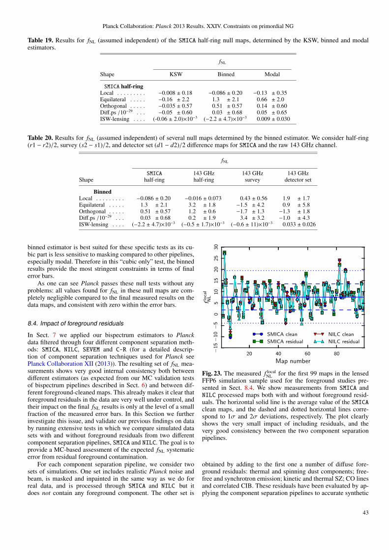
Planck Collaboration: Planck 2013 Results. XXIV. Constraints on primordial NG
Table 19. Results for fNL (assumed independent) of the SMICA half-ring null maps, determined by the KSW, binned and modalestimators.
fNL
Shape KSW Binned Modal
SMICA half-ringLocal . . . . . . . . . −0.008 ± 0.18 −0.086 ± 0.20 −0.13 ± 0.35Equilateral . . . . . −0.16 ± 2.2 1.3 ± 2.1 0.66 ± 2.0Orthogonal . . . . . −0.035 ± 0.57 0.51 ± 0.57 0.14 ± 0.60Diff.ps /10−29 . . . −0.05 ± 0.60 0.03 ± 0.68 0.05 ± 0.65ISW-lensing . . . . (-0.06 ± 2.0)×10−3 (−2.2 ± 4.7)×10−3 0.009 ± 0.030
Table 20. Results for fNL (assumed independent) of several null maps determined by the binned estimator. We consider half-ring(r1 − r2)/2, survey (s2 − s1)/2, and detector set (d1 − d2)/2 difference maps for SMICA and the raw 143 GHz channel.
fNL
SMICA 143 GHz 143 GHz 143 GHzShape half-ring half-ring survey detector set
BinnedLocal . . . . . . . . . −0.086 ± 0.20 −0.016 ± 0.073 0.43 ± 0.56 1.9 ± 1.7Equilateral . . . . . 1.3 ± 2.1 3.2 ± 1.8 −1.5 ± 4.2 0.9 ± 5.8Orthogonal . . . . . 0.51 ± 0.57 1.2 ± 0.6 −1.7 ± 1.3 −1.3 ± 1.8Diff.ps /10−29 . . . 0.03 ± 0.68 0.2 ± 1.9 3.4 ± 3.2 −1.0 ± 4.3ISW-lensing . . . . (−2.2 ± 4.7)×10−3 (−0.5 ± 1.7)×10−3 (−0.6 ± 11)×10−3 0.033 ± 0.026
binned estimator is best suited for these specific tests as its cu-bic part is less sensitive to masking compared to other pipelines,especially modal. Therefore in this “cubic only” test, the binnedresults provide the most stringent constraints in terms of finalerror bars.
As one can see Planck passes these null tests without anyproblems: all values found for fNL in these null maps are com-pletely negligible compared to the final measured results on thedata maps, and consistent with zero within the error bars.
8.4. Impact of foreground residuals
In Sect. 7 we applied our bispectrum estimators to Planckdata filtered through four different component separation meth-ods: SMICA, NILC, SEVEM and C-R (for a detailed descrip-tion of component separation techniques used for Planck seePlanck Collaboration XII (2013)). The resulting set of fNL mea-surements shows very good internal consistency both betweendifferent estimators (as expected from our MC validation testsof bispectrum pipelines described in Sect. 6) and between dif-ferent foreground-cleaned maps. This already makes it clear thatforeground residuals in the data are very well under control, andtheir impact on the final fNL results is only at the level of a smallfraction of the measured error bars. In this Section we furtherinvestigate this issue, and validate our previous findings on databy running extensive tests in which we compare simulated datasets with and without foreground residuals from two differentcomponent separation pipelines, SMICA and NILC. The goal is toprovide a MC-based assessment of the expected fNL systematicerror from residual foreground contamination.
For each component separation pipeline, we consider twosets of simulations. One set includes realistic Planck noise andbeam, is masked and inpainted in the same way as we do forreal data, and is processed through SMICA and NILC but itdoes not contain any foreground component. The other set is
20 40 60 80
Map number
−1
5−
10−
50
51
01
52
02
53
0
flo
cal
NL
SMICA clean
SMICA residual
NILC clean
NILC residual
Fig. 23. The measured f localNL for the first 99 maps in the lensed
FFP6 simulation sample used for the foreground studies pre-sented in Sect. 8.4. We show measurements from SMICA andNILC processed maps both with and without foreground resid-uals. The horizontal solid line is the average value of the SMICAclean maps, and the dashed and dotted horizontal lines corre-spond to 1σ and 2σ deviations, respectively. The plot clearlyshows the very small impact of including residuals, and thevery good consistency between the two component separationpipelines.
obtained by adding to the first one a number of diffuse fore-ground residuals: thermal and spinning dust components; free-free and synchrotron emission; kinetic and thermal SZ; CO linesand correlated CIB. These residuals have been evaluated by ap-plying the component separation pipelines to accurate synthetic
43

Planck Collaboration: Planck 2013 Results. XXIV. Constraints on primordial NG
Table 21. Summary of our fNL analysis of foreground residuals. For realistic lensed FFP6 simulations processed through the SMICAand NILC component separation pipelines, we report: the average fNL with and without foreground residuals added to the maps, thefNL standard deviation in the same two cases, and the standard deviation of the map-by-map fNL difference between the “clean” and“contaminated” sample. The impact of foreground residuals is clearly subdominant when compared to statistical error bars for allshapes. Results reported below have been obtained using the modal estimator.
fNL
SMICA SMICA NILC NILC SMICA NILCShape clean residual clean residual residual − clean residual − clean
ModalLocal . . . . . . . . . 7.7 ± 5.9 7.8 ± 5.9 7.7 ± 5.8 7.4 ± 6.0 0.04 ± 1.0 −0.27 ± 1.1Equilateral . . . . . −0.5 ± 77 −8.7 ± 79 −0.6 ± 78 −9.0 ± 79 −8.3 ± 8.2 −8.4 ± 8.3Orthogonal . . . . . −23 ± 41 −25 ± 41 −24 ± 40 −26 ± 41 −2.0 ± 4.7 −2.4 ± 4.8ISW-lensing . . . . 1.00 ± 0.38 1.01 ± 0.38 1.01 ± 0.38 1.02 ± 0.38 0.006 ± 0.052 0.013 ± 0.052
Planck datasets including foreground emission according to thePSM (Delabrouille et al. 2012), and are of course dependent onthe cleaning method adopted. The simple procedure of addingforeground residuals to the initially clean simulations is madepossible because we consider only linear component separationmethods for our analysis. Linearity is in general an importantrequirement for foreground cleaning algorithms aiming at pro-ducing maps suitable for NG analyses. All maps in both samplesare lensed using the LensPix algorithm. We analyse both setsusing different bispectrum estimators (modal, KSW, binned) forcross-validation purposes.
The presence of residual foreground components in the datacan have two main effects on the measured fNL. The first is to in-troduce a bias in the fNL measurements due to the correlation be-tween the foreground and primordial 3-point function for a givenshape. The second is to increase the error bars while leavingthe bispectrum estimator asymptotically unbiased. This is a con-sequence of accidental correlations between primordial CMBanisotropies and foreground emission. Of course these “CMB-CMB-foregrounds” bispectrum terms average to zero but theydo not cancel in the bispectrum variance 6-point function. Aninteresting point to note is that a large foreground three-pointfunction will tend to produce a negative bias in the local bispec-trum measurements. That is because foreground emission pro-duces a positive skewness of the CMB temperature distribution(“excess of photons”), and a positive skewness is in turn relatedto a negative f local
NL16. A large negative f local
NL is thus a signatureof significant foreground contamination in the map. This is in-deed what we observe if we consider raw frequency maps witha small Galactic cut, which is why our frequency-by-frequencyanalysis in Sect. 8.2 was performed using a very large mask. Formore details regarding effects of foreground contamination onprimordial NG measurements in the context of the WMAP anal-ysis see Yadav & Wandelt 2008 and Senatore et al. 2010.
In our test we built maps contaminated with foregroundresiduals by simply adding residual components to the cleanmaps. That means that the difference ( f residual
NL − f cleanNL )i for the i-th
realization in the simulated sample exactly quantifies the changein fNL due to foregrounds on that realization. In order to assessthe level of residual foreground contamination on primordial and
16 While not rigorous, this argument captures the leading effect sinceGalactic foregrounds predominantly contaminate large scales. In prin-ciple, positively skewed, small scale foreground residuals (` > 60), orthe negatively skewed SZ effect, can contribute positive bias. Our sim-ulations with foreground residuals demonstrate that these contributionsare subdominant.
ISW-lensing shapes, first of all we consider the difference be-tween average values and standard deviations of fNL measuredfrom the two map samples for each shape. As shown in Table 21we find that neither the average nor the standard deviation showsa significant change between the two datasets. That means thatforeground residuals are clearly subdominant, as they do not biasthe estimator for any shape and they do not increase the variancethrough spurious correlations with the CMB primordial signal.
We also consider the difference f residualNL − f clean
NL on a map-by-map basis and compute its standard deviation. This is used as anestimate of the expected bias on a single realization due to thepresence of residuals. As already expected from the negligiblechange in the standard deviations of the two samples, the vari-ance of the map-by-map differences is also very small: Table 21again shows that it is at most about σ fNL/6 for any given shape,where σ fNL is the fNL standard deviation for that shape. As anexample, in Fig. 23 we show the measured values of f local
NL forthe first 99 maps in both the SMICA and NILC samples, compar-ing results with and without residuals. It is evident also from thisplot that the change in central value due to including residuals isvery small. The very good agreement between the two compo-nent separation pipelines is also worth notice.
From the study shown here and from the comparison be-tween different component separation methods in Sect. 7, we canthus conclude that the combination of foreground-cleaned mapsand fsky = 0.73 sky coverage we adopt in this work provide avery robust choice for fNL studies.
8.5. Impact of HFI time-ordered information processing onNG constraints
Our validation tests are designed to determine whether instru-mental or data processing systematics could lead to a spuriousdetection of primordial NG. Our analysis protocol passes thesetests which allows us to rule out this concern with confidence.These validation tests do not exclude the possibility that the ex-tensive processing of HFI time-ordered information (TOI) couldsomehow remove non-Gaussian signals present on the sky andthus negatively impact Planck’s ability to detect them. If thiswere true it would weaken the bounds on primordial NG re-ported here. HFI TOI processing includes glitch fitting, gain driftand correction (ADC non-linearity), 4K cooler line removal,telegraph noise step correction, and TOD filtering to correctfor the bolometer time constant (Planck Collaboration VI 2013;Planck Collaboration VII 2013; Planck Collaboration X 2013).
44

Planck Collaboration: Planck 2013 Results. XXIV. Constraints on primordial NG
The following facts constitute strong evidence that HFI TOIprocessing does not remove non-Gaussian signals:
1. Planck’s 2.6σ ISW-lensing bispectrum measurement is con-sistent with expectations from the LCDM model, and hasthe right skew-C` shape. Like NG of local type, this is asqueezed bispectrum template.
2. When frequency maps are combined to maximize the CIBsignal, Planck finds a 25σ detection of the nearly squeezedCIB-lensing bispectrum, consistent with the CIB 2-pointcorrelations inferred by Planck (Planck Collaboration XXX2013).
3. Planck detects residual point sources in the SMICA maps at5σ, seen as a bispectrum of equilateral shape at high ` con-sistent with the expected skew-spectrum shape (Fig. 2) onthe angular scales where residual infrared sources and far in-frared background are expected to be the dominant contam-inants of the power spectrum according to the foregroundresiduals in FFP6 simulations of SMICA maps (Fig. E.3 inPlanck Collaboration XII 2013).
4. The trispectrum signal imprinted by Planck’s motion withrespect to the CMB rest frame is seen at a sensible level andin a plausible direction (Planck Collaboration XXVII 2013).
5. Planck detects the trispectrum signal due to lensing by largescale structure with high significance and in accordance withLCDM predictions based on the Planck parameter likeli-hood.
6. Fig. 22 shows that we reproduce the WMAP-9 local NG re-sults on those larger angular scales where the WMAP-9 dataare cosmic variance limited.
We conclude that all the forms of NG that should have been seenby Planck have been seen, in quantitative agreement with theexpected level across the entire range of angular scales probed.While it cannot be excluded with absolute certainty that someunknown aspect of HFI TOI processing could have affectedsome unknown form of NG, the presence of these non-Gaussianfeatures in the resulting maps (in addition to signals such asthe extracted map of y-distortion, and galactic and extragalac-tic foregrounds), gives us confidence in the force of the boundson primordial NG described in this paper.
9. Implications for early Universe physics
The NG analyses performed in this paper show that Planck dataare consistent with Gaussian primordial fluctuations. The stan-dard models of single-field slow-roll inflation have thereforesurvived the most stringent tests of Gaussianity performed todate. On the other hand, the NG constraints obtained on dif-ferent primordial bispectrum shapes (e.g., local, equilateral andorthogonal), after properly accounting for various contaminants,severely limit various classes of mechanisms for the generationof the primordial perturbations proposed as alternatives to thestandard models of inflation.
In the following subsections, unless explicitly stated oth-erwise, we translate limits on NG to limits on parametersof the theories by constructing a posterior assuming the fol-lowing: the sampling distribution is Gaussian (which is sup-ported by Gaussian simulations); the likelihood is approximatedby the sampling distribution but centred on the NG estimate(see Elsner & Wandelt 2009); uniform or Jeffreys’ prior (wherestated), over ranges which are physically meaningful, or as oth-erwise stated. Where two parameters are involved, the posterioris marginalized to give one-dimensional constraints on the pa-rameter of interest.
9.1. General single-field models of inflation
DBI models: The constraints on f equilNL provide constraints on
the sound speed with which the inflaton fluctuations can prop-agate during inflation. For example, for DBI models of infla-tion (Silverstein & Tong 2004; Alishahiha et al. 2004), wherethe inflaton field features a non-standard kinetic term, thepredicted value of the nonlinearity parameter is f DBI
NL =
−(35/108)(c−2s − 1) (Silverstein & Tong 2004; Alishahiha et al.
2004; Chen et al. 2007b). Although very similar to the equilat-eral shape, we have obtained constraints directly on the theo-retical (nonseparable) predicted shape (Eq. 7)). The constraintf DBINL = 11 ± 69 at 68% CL (see Eq. (86)) implies
cDBIs ≥ 0.07 95% CL . (95)
The DBI class contains two possibilities based on string con-structions. In ultraviolet (UV) DBI models, the inflaton fieldmoves under a quadratic potential from the UV side of a warpedbackground to the infrared side. It is known that this case is al-ready at odds with observations, if theoretical internal consis-tency of the model and constraints on power spectra and primor-dial NG are taken into account (Baumann & McAllister 2007;Lidsey & Huston 2007; Bean et al. 2007; Peiris et al. 2007). Ourresults strongly limit the relativistic regime of these models evenwithout applying the theoretical consistency constraints.
It is therefore interesting to look at infrared (IR) DBI mod-els (Chen 2005b,a) where the inflaton field moves from the IR tothe UV side, and the inflaton potential is V(φ) = V0 −
12βH2φ2,
with a wide range 0.1 < β < 109 allowed in principle. Inprevious work (Bean et al. 2008) a 95% CL limit of β < 3.7was obtained using WMAP. In a minimal version of IR DBI,where stringy effects are neglected and the usual field the-ory computation of the primordial curvature perturbation holds,one finds (Chen 2005c; Chen et al. 2007b) cs ' (βN/3)−1,ns − 1 = −4/N, where N is the number of e-folds; further,primordial NG of the equilateral type is generated with anamplitude f DBI
NL = −(35/108) [(β2 N2/9) − 1]. For this model,the range N ≥ 60 is compatible with Planck’s 3σ limits onns (Planck Collaboration XXII 2013). Marginalizing over 60 ≤N ≤ 90, we find
β ≤ 0.7 95% CL , (96)
dramatically restricting the allowed parameter space of thismodel.
Power-law k-inflation: These models (Armendariz-Picon et al.1999; Chen et al. 2007b) predict f equil
NL = −170/(81γ), wherens − 1 = −3γ, c2
s ' γ/8. Assuming a prior of 0 < γ < 2/3,our constraint f equil
NL = −42 ± 75 at 68% CL (see Table 9)leads to the limit γ ≥ 0.05 at 95% CL. On the other hand,Planck’s constraint on ns − 1 yields the limit 0.01 ≤ γ ≤0.02 (Planck Collaboration XXII 2013). These conflicting lim-its severely constrain this class of models.
Flat Models and higher derivative interactions: Flat NG cancharacterize inflationary models which arise from independentinteraction terms different from the (π)3 and π(∇π)2 discussedin Sect. 2 (see also Sect. 9.2). An example is given by mod-els of inflation based on a Galilean symmetry (Creminelli et al.2011a), where one of the inflaton cubic interaction terms allowedby the Galilean symmetry, M3[π(∂i∂ jπ)2/a4 − 2Hππ2 + 3H3π3],contributes to the flat bispectrum with an amplitude f flat
NL =
(35/256)(M3H)/(εM2Pl) (Creminelli et al. 2011a). Here, π is the
relevant inflaton scalar degree of freedom, ε the usual slow-roll
45

Planck Collaboration: Planck 2013 Results. XXIV. Constraints on primordial NG
parameter and a the scale factor and H the Hubble parame-ter during inflation. Our constraint f flat
NL = 37 ± 77 at 68% CL(see Table 11) leads to (M3H)/(εM2
Pl) = 270 ± 563 at 68%CL. These interaction terms are similar to those arising in gen-eral inflaton field models that include extrinsic curvature terms,e.g., parameterized in the Effective Field Theory approach asM2π(∂i jπ)2/a4 (Bartolo et al. 2010a), which contribute to a flatbispectrum with an amplitude f flat
NL = (50/108) M2/(c2s εM2
Pl). Inthis case, we obtain M2/(c2
s εM2Pl) = 80 ± 166 at 68% CL.
9.2. Implications for Effective Field Theory of Inflation
The effective field theory approach to inflation (Weinberg 2008;Cheung et al. 2008) provides a general way to scan the NG pa-rameter space of inflationary perturbations. For example, onecan expand the Lagrangian of the dynamically relevant degreesof freedom into the dominant operators satisfying some under-lying symmetries. We will focus on general single-field modelsparametrized by the following operators (up to cubic order)
S =
∫d4x√−g
−M2PlH
c2s
(π2 − c2
s(∂iπ)2
a2
)(97)
− M2PlH(1 − c−2
s )π(∂iπ)2
a2 +
(M2
PlH(1 − c−2s ) −
43
M43
)π3
]where π is the scalar degree of freedom (ζ = −Hπ). The mea-surements on f equil
NL and f orthoNL can be used to constrain the mag-
nitude of the inflaton interaction terms π(∂iπ)2 and (π)3 whichgive respectively f EFT1
NL = −(85/324)(c−2s − 1) and f EFT2
NL =
−(10/243)(c−2s − 1)
[c3 + (3/2)c2
s
](Senatore et al. 2010, see also
Chen et al. 2007b; Chen 2010b). These two operators give riseto shapes that peak in the equilateral configuration that are,nevertheless, slightly different, so that the total NG signal willbe a linear combination of the two, possibly leading also toan orthogonal shape. There are two relevant NG parameters,cs, the sound speed of the the inflaton fluctuations, and M3which characterizes the amplitude of the other operator π3.Following Senatore et al. (2010) we will focus on the dimension-less parameter c3(c−2
s − 1) = 2M43c2
s/(HM2Pl). For example, DBI
inflationary models corresponds to c3 = 3(1 − c2s )/2, while the
non-interacting model (vanishing NG) correspond to cs = 1 andM3 = 0 (or c3(c−2
s − 1) = 0).The mean values of the estimators for equilateral and orthog-
onal NG amplitudes are given in terms of cs and c3 by
f equilNL =
1 − c2s
c2s
(−0.275 + 0.0780A)
f orthoNL =
1 − c2s
c2s
(0.0159 − 0.0167A) (98)
where A = −(c2s + (2/3)c3), and the coefficients are com-
puted from the Fisher correlation matrix between the equilat-eral and orthogonal template bispectra and the theoretical bis-pectra arising from the two operators π(∇π)2 and π3. Givenour constraints on f equil
NL and f orthoNL , and the covariance matrix
C of the joint estimators, we can define a χ2 statistic given byχ2(c3, cs) = uT (c3, cs)C−1u(c3, cs), where the vector u is givenby vi(c3, cs) = f i(c3, cs) − f i
P. f iP, where i={equilateral, orthog-
onal}, are the joint estimates of the equilateral and orthogonalfNL measured by Planck and f i(c3, cs) is given by Eq. (98).Figure 24 shows the 68%, 95%, and 99.7% confidence regions
�300 �200 �100 0 100 200 300
f equilNL
�200
�100
0100
200
fort
ho
NL
Fig. 24. 68%, 95%, and 99.7% confidence regions in the param-eter space ( f equil
NL , f orthoNL ), defined by thresholding χ2 as described
in the text.
10�2 10�1 100
cs
�20000
�10000
010000
c 3(c�
2s�
1)
Fig. 25. 68%, 95%, and 99.7% confidence regions in the single-field inflation parameter space (cs, c3), obtained from Fig. 24 viathe change of variables in Eq. (98).
for f equilNL and f ortho
NL , obtained by requiring χ2 ≤ 2.28, 5.99, and11.62 respectively, as appropriate for a χ2 variable with two de-grees of freedom. The corresponding confidence regions in the(c3, cs) parameter space are shown in Fig. 25. After marginal-izing over c3 we find the following conservative bound on theinflaton sound-speed
cs ≥ 0.02 95% CL . (99)
Note that we have also looked explicitly for the non-separableshapes in Sect. 7.3.1, in particular the two effective field theoryshapes and the DBI inflation shape (see Eqs. (5, 6, 7)) .
46

Planck Collaboration: Planck 2013 Results. XXIV. Constraints on primordial NG
9.3. Multi-field models
Curvaton models: Planck NG constraints have interesting im-plications for the simplest adiabatic curvaton models. They pre-dict (Bartolo et al. 2004d,c)
f localNL =
54rD−
5rD
6−
53, (100)
for a quadratic potential of the curvaton field (Lyth & Wands2002; Lyth et al. 2003; Lyth & Rodriguez 2005; Malik & Lyth2006; Sasaki et al. 2006), where rD = [3ρcurvaton/(3ρcurvaton +4ρradiation)]D is the “curvaton decay fraction” evaluated at theepoch of the curvaton decay in the sudden decay approxima-tion. Assuming a prior 0 < rD < 1, given our constraintf localNL = 2.7 ± 5.8 at 68% CL, we obtain
rD ≥ 0.15 95% CL . (101)
In Planck Collaboration XXII (2013) a limit on rD is derivedfrom the constraints on isocurvature perturbations under the as-sumption that there is some residual isocurvature fluctuations inthe curvaton field. For this restricted case, they find rD > 0.98(95% CL), compatible with the constraint obtained here.
Quasi-single field inflation: It is beyond the scope of this pa-per to perform a general multi-field analysis employing the localNG constraints. However, we have performed a detailed anal-ysis for the quasi-single field models (see Eq. (12)). Quasi-single field (QSF) inflation models (Chen & Wang 2010b,a;Baumann & Green 2012) are a natural consequence of inflationmodel-building in string theory and supergravity (see Sect. 2.2).In addition to the inflaton field, these models have extra fieldswith masses of order the Hubble parameter, which are stabilizedby supersymmetry. A distinctive observational signature of thesemassive fields is a one-parameter family of large NG whosesqueezed limits interpolate between the local and the equilat-eral shape. Therefore, by measuring the precise momentum-dependence of the squeezed configurations in the NG, in prin-ciple, we are directly measuring the parameters of the theorynaturally determined by the fundamental principle of supersym-metry. These models produce a bispectrum (Eq. (12)) dependingon two parameters ν, f QSI
NL , with a shape that interpolates betweenthe local shape, where ν = 1.5 and the equilateral shape, whereν = 0.
Results are shown in Fig. 26 (see Sect. 7.3.6 for details ofthe analyses). The best fit value corresponds to ν = 1.5, fNL =4.79 which would imply, within this scenario, that the extra fielddifferent from the inflaton has a mass m � H. However, thefigure shows that there is no preferred value for ν with all valuesallowed at 3σ.
9.4. Non-standard inflation models
Constraints on excited initial states: Results from Sect. 7.3 con-strain a variety of models with flattened bispectra, often incombination with a non-trivial squeezed limit. The most no-table examples are bispectra produced in excited initial statemodels (non-Bunch-Davies vacua), which can be generated bystrong disturbances away from background slow-roll evolu-tion or additional trans-Planckian physics (Chen et al. 2007b;Holman & Tolley 2008; Meerburg et al. 2009; Agullo & Parker2011). The constraints we have obtained are summarized inTable 11, and cover four representative cases (see Eq. (14, 15))in the literature. We find no strong evidence for these flattenedbispectra in the Planck data after subtraction of the ISW-lensing
0
0
.3
0.
6
0.
9
1.2
1.5
f N L
ν
f N L
ν
f N L
ν
NL
ν
NL
ν
NL
ν
NL
ν
NLNL-100 −50 0 50 100
fNLQSF
νFig. 26. 68%, 95%, and 99.7% confidence intervals for ν andf QSINL for quasi-single field inflation. The best fit value of ν = 1.5,
f QSINL = 4.75 is marked with an X. The contours were calculated
using MC methods by creating 2 × 10⁹ simulations using the βcovariance matrix around this best fit model.
signal, with which all these models have some correlation. Thisis consistent with an earlier constraint on the NBD model fromWMAP (Fergusson et al. 2012). However, this investigation islimited by the present resolution of the polynomial modal es-timator (nmax = 600), so more strongly flattened models are notexcluded by this analysis.
Directional dependence motivated by fields: Directionally-dependent bispectra (Eq. (19)), motivated by inflation withgauge fields, have also been constrained (see Table 11). For ex-ample, models with a kinetic term of the vector field(s) L =−I2(φ)F2/4, where F2 is the strength of the gauge field, and I(φ)is a function of the inflaton field which, with an appropriate timedependence (see, e.g., Ratra 1992), can generate vector fieldsduring inflation. For these models the L = 0, 2 modes in thebispectrum are excited with f L
NL = XL(|g∗|/0.1) (Nk3/60), whereXL=0 = (80/3) and XL=2 = −(10/6), respectively (Barnaby et al.2012a; Bartolo et al. 2013; Shiraishi et al. 2013). Here g∗ is theamplitude of a quadrupolar anisotropy in the power spectrum(see, e.g., Ackerman et al. (2007)) and N is the number of e-folds before the end of inflation when the relevant scales exitthe horizon. These modes therefore relate the bispectrum am-plitude to the level of statistical anisotropy in the power spec-trum. Marginalizing over a prior 50 ≤ N ≤ 70 assuming uni-form priors on g∗, our constraints in Table 11 lead to the limits−0.05 < g∗ < 0.05 and −0.36 < g∗ < 0.36 from the L = 0, L = 2modes respectively (95% CL). Note, however, that in the currentanalysis only a modest correlation was possible with the shapecorresponding to the L = 2 mode. These results apply to all mod-els where curvature perturbations are sourced by a I2(φ)F2 term(see references in Shiraishi et al. 2013).
Feature models: Non-scale-invariant oscillatory bispectrumshapes can be generated by sharp or periodic features in the
47
Planck Collaboration: Planck 2013 Results. XXIV. Constraints on primordial NG
inflaton potential, with particular recent interest on axion mon-odromy models motivated by string theory (see Sect. 2.3). Wehave undertaken a survey of simple feature models (Eq. (16))which have a periodicity accessible to the polynomial modalestimator (wavenumbers K = k1 + k2 + k3 & 0.01), a two-parameter space spanned by K and a phase φ. There are inter-esting best fit models for the Planck CMB bispectrum aroundK = 0.01875, φ = 0 (that is, with a large-` bispectrum pe-riodicity around ∆` = 260), with results shown in Table 12.We note important caveats on the statistics of parameter sur-veys like this in Sect. 7.3.3; given the large numbers of featuremodels studied, we have to apply a higher threshold for statis-tical significance as shown for a survey of 200 Gaussian sim-ulations. This feature survey takes forward earlier results forthe WMAP data (Fergusson et al. 2012), with the apparent fitreflecting the signal observed in the Planck CMB reconstruc-tion (see Fig. 7). Most attention on feature models has beenmotivated by the simplest single-field case for which there arecorrelated signals predicted in the bispectrum and power spec-trum (see e.g., Chen et al. 2007a; Adshead et al. 2012). In thiscase, regions with small k ∼ 0.001 are favoured for producingan observable bispectrum17, given existing WMAP power spec-trum constraints on these models. Periodicities ∆` . 20 areanticipated (see Adshead et al. 2012) which are not accessibleto the present modal bispectrum estimator analysis, but whichare discussed in (Planck Collaboration XXII 2013). Conversely,the Planck feature model survey using the power spectrum(Planck Collaboration XXII 2013) does cover bispectrum scalesand parameters investigated in this paper. An analysis ofthe Bayesian posterior probability (Planck Collaboration XXII2013) does not appear to provide evidence favoring parametersassociated with the current best-fit bispectrum model. More de-tailed analysis using the specific bispectrum envelope for thesingle-field feature solution is being undertaken.
Resonance models: We have also investigated resonance modelsof Eq. (17) such as axion monodromy and enfolded resonancemodels of Eq. (18), in which non-Bunch-Davies vacua are ex-cited by sharp features. This limited analysis focuses on period-icities associated with the best-fit feature model and the resultsare described in Tables C.1 and C.2. No significant signal wasfound in this domain for either of these two models. However,we note that the logarithmic dependence of the bispectrum cre-ates challenges at low k, as we must ensure important featuresdo not fall below the modal resolution. This restricts the presentsurvey range, which will be extended in future. Again, we notethat most attention on these models has focused on higher `-periodicities than those accessible to the present modal estima-tor (see e.g., Flauger & Pajer 2011; Peiris et al. 2013), for thesame reason as the feature models. A resonance model surveyusing the Planck power spectrum has been undertaken and theresults can be found in Planck Collaboration XXII (2013); how-ever, this also currently excludes high frequencies that have re-ceived attention in the literature.
Warm inflation: This model, where dissipative effects are impor-tant, predicts f warm
NL = −15 ln (1 + rd/14) − 5/2 (Moss & Xiong2007) where the dissipation parameter rd = Γ/(3H) must belarge for strong dissipation. The limit from WMAP is rd ≤ 2.8 ×10⁴ (Moss & Xiong 2007). Assuming a prior 0 ≤ log10 rd ≤ 4,
17 Planck Collaboration XVI (2013) confirms an anomaly in thepower spectrum at 20 . ` . 40 first noted in WMAP, which leads to animprovement in likelihood when fitted with a feature in the inflationarypotential (Peiris et al. 2003). Unfortunately, the best-fit parameters inthis case do not lead to an observable bispectrum (Adshead et al. 2011).
our constraint f warmSNL = 4 ± 33 at 68% CL (see Sect. 7.3.5)
yields a limit on the dissipation parameter of log10 rd ≤ 2.6(95% CL), improving the previous limit by nearly two ordersof magnitude. The strongly-dissipative regime with rd & 2.5 stillremains viable; however, the Planck constraint puts the modelin a regime which can lead to an overproduction of gravitinos(see Hall & Peiris (2008) and references within).
9.5. Alternatives to inflation
Perhaps the most striking example is given by the ekpy-rotic/cyclic models (for a review, see Lehners 2010) proposedas alternative to inflationary models. Typically they predict alocal NG | f local
NL | > 10. In particular, the so-called “ekpyroticconversion” mechanism (in which isocurvature perturbationsare converted into curvature perturbations during the ekpyroticphase) yields f local
NL = −(5/12) c21, where c1 is a parameter in
the potential, requiring 10 & c1 & 20 for compatibility withpower spectrum constraints. This case was ∼ 4σ discrepant withWMAP data, and with Planck it is decisively ruled out givenour bounds f local
NL = 2.7 ± 5.8 at 68% CL (see Table 9) yield-ing c1 ≤ 4.2 at 95% CL. The predictions for the local bispec-trum from other ekpyrotic models (based on the so called “ki-netic conversion” taking place after the ekpyrotic phase) yieldf localNL = (3/2) κ3
√ε ± 5, where values −1 < κ3 < 5 and ε ∼ 100
are natural (Lehners 2010). Taking ε ∼ 100, in this case we ob-tain −0.9 < κ3 < 0.6 and −0.2 < κ3 < 1.3 at 95% CL, for theplus and minus sign in f local
NL respectively, significantly restrictingthe viable parameter space of this model.
9.6. Implications of CMB trispectrum results
The non-detection of local-type fNL by Planck raises the imme-diate question of whether there might still be a large trispec-trum. In this first analysis we have focused on the local shapeτNL. Most inflation models predict τNL ∼ O( f 2
NL) (Byrnes et al.2006; Elliston et al. 2012), and hence given our tight fNL limits,would be predicted to be very small. This is easily consistentwith our conservative upper limit τNL < 2800, and also withthe significantly smaller signals found in the modulation dipoleand quadrupole. Our upper limit also restricts the freedom ofcurvaton-like models with quadratic terms that are nearly uncor-related with the curvature perturbation, which could in principlehave fNL ∼ 0 but a large trispectrum (Byrnes & Choi 2010).
10. Conclusions
In this paper we have derived constraints on primordial NG, us-ing the CMB maps derived from the Planck nominal missiondata. Using three optimal bispectrum estimators – KSW, binned,and modal – we obtained consistent values for the primordiallocal, equilateral, and orthogonal bispectrum amplitudes, quot-ing as our final result f local
NL = 2.7 ± 5.8, f equilNL = −42 ± 75,
and f orthoNL = −25 ± 39 (68 % CL statistical). Hence there is
no evidence for primordial NG of one of these shapes. We did,however, measure the ISW-lensing bispectrum expected in theΛCDM scenario, as well as a contribution from diffuse pointsources, and these contributions are clearly seen in the form ofthe associated skew-C`. Indeed, the detection of ISW-lensingand Poisson point source skew-C` with the right shapes and atexpected levels is good evidence that the data processing is notdestroying non-gaussianity in the maps, and gives confidencethat the non-detections of primordial non-gaussianity are robust.
48

Planck Collaboration: Planck 2013 Results. XXIV. Constraints on primordial NG
These results have been confirmed by measurements using thewavelet bispectrum, and Minkowski functional estimators, anddemonstrated to be stable for the four different component sep-aration techniques SMICA, NILC, SEVEM, and C-R, showing theirrobustness against foreground residuals. They have also passedan extensive suite of tests studying the dependence on the max-imum multipole number and the mask, consistency checks be-tween frequency channels, and several null tests. In addition,we have summarized in this paper an extensive validation cam-paign for the three optimal bispectrum estimators on Gaussianand non-Gaussian simulations.
Extending our analysis beyond estimates of individualshape amplitudes, we presented model-independent, three-dimensional reconstructions of the Planck CMB bispectrum us-ing the modal and binned bispectrum estimators. These resultswere also shown to be fully consistent between the differentcomponent separation techniques even for the full bispectrum,and contained no significant NG signals of a type not capturedby our standard templates at low multipole values. At high mul-tipoles, some indications of unidentified NG signals were found,as also evidenced by the results from the skew-C` estimator.Further study will be required to ascertain whether these indi-cations are due to foreground residuals, beams, data processing,or a more interesting signal.
Using the modal decomposition, we have presented con-straints on key primordial NG scenarios, including generalsingle-field models with non-separable shapes, excited initialstates (non-Bunch-Davies vacua), and directionally-dependentvector models. We have also undertaken an initial survey ofscale-dependent feature and resonance models.
Moving beyond three-point correlations, we have obtainedlimits from the Planck data on the amplitude of the local four-point function. Our trispectrum reconstruction yielded a signalconsistent with zero except for an anomalously large octopole.Frequency dependence indicated that this was unlikely to be pri-mordial, but allowing the signal to be primordial we placed anupper limit τNL < 2800 (95% CL).
We have discussed the impact of these results on the infla-tionary model space, and derived bispectrum constraints on a se-lection of specific inflationary mechanisms, including both gen-eral single-field inflationary models (extensions to the standardsingle-field slow-roll case) and multi-field models. Our resultsled to a lower bound on the speed of sound, cs ≥ 0.02 (95%CL), in an effective field theory approach to inflationary modelswhich includes models with non-standard kinetic terms. Strongconstraints on other scenarios such as IR DBI, k-inflation, infla-tionary models involving gauge fields, and warm inflation havebeen obtained. Within the class of multi-field models, our mea-surements limit the curvaton decay fraction to rD ≥ 0.15 (95%CL). Ekpyrotic/cyclic scenarios were shown to be under pres-sure from the Planck data: we robustly ruled out the so-called“ekpyrotic conversion” mechanism, and found that the parame-ter space of the “kinetic conversion” mechanism is significantlylimited.
With these results, the paradigm of standard single-fieldslow-roll inflation has survived its most stringent tests to-date.
Acknowledgements. The development of Planck has been supported by:ESA; CNES and CNRS/INSU-IN2P3-INP (France); ASI, CNR, and INAF(Italy); NASA and DoE (USA); STFC and UKSA (UK); CSIC, MICINN,JA and RES (Spain); Tekes, AoF and CSC (Finland); DLR and MPG(Germany); CSA (Canada); DTU Space (Denmark); SER/SSO (Switzerland);RCN (Norway); SFI (Ireland); FCT/MCTES (Portugal); and PRACE (EU).A description of the Planck Collaboration and a list of its members,including the technical or scientific activities in which they have beeninvolved, can be found at http://www.sciops.esa.int/index.php?
project=planck&page=Planck_Collaboration. The primary platform foranalysis with the modal and KSW estimators was the COSMOS supercom-puter, part of the DiRAC HPC Facility supported by STFC and the UK LargeFacilities Capital Fund. We gratefully acknowledge IN2P3 Computer Center(http://cc.in2p3.fr) for providing a significant amount of the computing resourcesand services needed for the analysis with the binned bispectrum estimator. Thisresearch used resources of the National Energy Research Scientific ComputingCenter, which is supported by the Office of Science of the U.S. Department ofEnergy under Contract No. DE-AC02-05CH11231. We acknowledge the use ofresources from the Norewegian national super computing facilities NOTUR. Wealso acknowledge the IAP magique3 computer facilities as well as the curva-ton computer at the Department of Physics of the University of Illinois (Urbana,IL). We further acknowledge the computer resources and technical assistanceprovided by the Spanish Supercomputing Network nodes at Universidad deCantabria and Universidad Politecnica de Madrid as well as the support providedby the Advanced Computing and e-Science team at IFCA.
ReferencesAchucarro, A., Gong, J.-O., Hardeman, S., Palma, G. A., & Patil, S. P. 2011, J.
Cosmology Astropart. Phys., 1, 30, arXiv:1010.3693Ackerman, L., Carroll, S. M., & Wise, M. B. 2007, Phys. Rev. D, 75, 083502,
arXiv:astro-ph/0701357Acquaviva, V., Bartolo, N., Matarrese, S., & Riotto, A. 2003, Nuclear Physics B,
667, 119, arXiv:astro-ph/0209156Adshead, P., Dvorkin, C., Hu, W., & Lim, E. A. 2012, Phys. Rev. D, 85, 023531,
arXiv:1110.3050Adshead, P., Hu, W., Dvorkin, C., & Peiris, H. V. 2011, Phys. Rev. D, 84, 043519,
arXiv:1102.3435Agullo, I. & Parker, L. 2011, General Relativity and Gravitation, 43, 2541,
arXiv:1106.4240Alishahiha, M., Silverstein, E., & Tong, D. 2004, Phys. Rev. D, 70, 123505,
arXiv:hep-th/0404084Allen, T. J., Grinstein, B., & Wise, M. B. 1987, Physics Letters B, 197, 66Amendola, L., Catena, R., Masina, I., et al. 2011, J. Cosmology Astropart. Phys.,
7, 27, arXiv:1008.1183Antoine, J.-P. & Vandergheynst, P. 1998, Journal of Mathematical Physics, 39,
3987Arkani-Hamed, N., Creminelli, P., Mukohyama, S., & Zaldarriaga, M. 2004, J.
Cosmology Astropart. Phys., 4, 1, arXiv:hep-th/0312100Armendariz-Picon, C., Damour, T., & Mukhanov, V. 1999, Physics Letters B,
458, 209, arXiv:hep-th/9904075Arroja, F., Mizuno, S., & Koyama, K. 2008, J. Cosmology Astropart. Phys., 8,
15, arXiv:0806.0619Arroja, F., Mizuno, S., Koyama, K., & Tanaka, T. 2009, Phys. Rev. D, 80,
043527, arXiv:0905.3641Ashoorioon, A. & Shiu, G. 2011, J. Cosmology Astropart. Phys., 3, 25,
arXiv:1012.3392Assassi, V., Baumann, D., & Green, D. 2012, J. Cosmology Astropart. Phys., 11,
47, arXiv:1204.4207Babich, D. 2005, Phys. Rev. D, 72, 043003, arXiv:astro-ph/0503375Babich, D., Creminelli, P., & Zaldarriaga, M. 2004, J. Cosmology Astropart.
Phys., 8, 9, arXiv:astro-ph/0405356Bardeen, J. M. 1980, Phys. Rev. D, 22, 1882Barnaby, N. & Cline, J. M. 2006, Phys. Rev. D, 73, 106012, arXiv:astro-
ph/0601481Barnaby, N. & Cline, J. M. 2008, J. Cosmology Astropart. Phys., 6, 30,
arXiv:0802.3218Barnaby, N., Namba, R., & Peloso, M. 2011, J. Cosmology Astropart. Phys., 4,
9, arXiv:1102.4333Barnaby, N., Namba, R., & Peloso, M. 2012a, Phys. Rev. D, 85, 123523,
arXiv:1202.1469Barnaby, N., Pajer, E., & Peloso, M. 2012b, Phys. Rev. D, 85, 023525,
arXiv:1110.3327Barnaby, N. & Peloso, M. 2011, Physical Review Letters, 106, 181301,
arXiv:1011.1500Bartolo, N., Fasiello, M., Matarrese, S., & Riotto, A. 2010a, J. Cosmology
Astropart. Phys., 8, 8, arXiv:1004.0893Bartolo, N., Fasiello, M., Matarrese, S., & Riotto, A. 2010b, J. Cosmology
Astropart. Phys., 9, 35, arXiv:1006.5411Bartolo, N., Komatsu, E., Matarrese, S., & Riotto, A. 2004a, Phys. Rep., 402,
103, arXiv:astro-ph/0406398Bartolo, N., Matarrese, S., Peloso, M., & Ricciardone, A. 2013, Phys. Rev. D,
87, 023504, arXiv:1210.3257Bartolo, N., Matarrese, S., & Riotto, A. 2002, Phys. Rev. D, 65, 103505,
arXiv:hep-ph/0112261
49
Planck Collaboration: Planck 2013 Results. XXIV. Constraints on primordial NG
Bartolo, N., Matarrese, S., & Riotto, A. 2004b, J. Cosmology Astropart. Phys.,1, 3, arXiv:astro-ph/0309692
Bartolo, N., Matarrese, S., & Riotto, A. 2004c, Physical Review Letters, 93,231301, arXiv:astro-ph/0407505
Bartolo, N., Matarrese, S., & Riotto, A. 2004d, Phys. Rev. D, 69, 043503,arXiv:hep-ph/0309033
Bartolo, N., Matarrese, S., & Riotto, A. 2005, J. Cosmology Astropart. Phys., 8,10, arXiv:astro-ph/0506410
Bartolo, N., Matarrese, S., & Riotto, A. 2010c, Advances in Astronomy, 2010,arXiv:1001.3957
Bartolo, N., Matarrese, S., & Riotto, A. 2012, J. Cosmology Astropart. Phys., 2,17, arXiv:1109.2043
Bartolo, N. & Riotto, A. 2009, J. Cosmology Astropart. Phys., 3, 17,arXiv:0811.4584
Baumann, D. & Green, D. 2012, Phys. Rev. D, 85, 103520, arXiv:1109.0292Baumann, D. & McAllister, L. 2007, Phys. Rev. D, 75, 123508, arXiv:hep-
th/0610285Bean, R., Chen, X., Peiris, H., & Xu, J. 2008, Phys. Rev. D, 77, 023527,
arXiv:0710.1812Bean, R., Shandera, S. E., Tye, S.-H. H., & Xu, J. 2007, J. Cosmology Astropart.
Phys., 5, 4, arXiv:hep-th/0702107Bennett, C. L., Larson, D., Weiland, J. L., et al. 2012, ArXiv e-prints,
arXiv:1212.5225Berera, A. 1995, Physical Review Letters, 75, 3218, arXiv:astro-ph/9509049Bernardeau, F., Kofman, L., & Uzan, J.-P. 2004, Phys. Rev. D, 70, 083004,
arXiv:astro-ph/0403315Bernardeau, F. & Uzan, J.-P. 2002, Phys. Rev. D, 66, 103506, arXiv:hep-
ph/0207295Bond, J. R., Frolov, A. V., Huang, Z., & Kofman, L. 2009, Physical Review
Letters, 103, 071301, arXiv:0903.3407Boubekeur, L., Creminelli, P., D’Amico, G., Norena, J., & Vernizzi, F. 2009, J.
Cosmology Astropart. Phys., 8, 29, arXiv:0906.0980Bucher, M., van Tent, B., & Carvalho, C. S. 2010, MNRAS, 407, 2193,
arXiv:0911.1642Bucher, M. & Zhu, Y. 1997, Phys. Rev. D, 55, 7415, arXiv:astro-ph/9610223Byrnes, C. T. & Choi, K.-Y. 2010, Advances in Astronomy, 2010,
arXiv:1002.3110Byrnes, C. T., Sasaki, M., & Wands, D. 2006, Phys. Rev. D, 74, 123519,
arXiv:astro-ph/0611075Cardoso, J., Martin, M., Delabrouille, J., Betoule, M., & Patanchon, G. 2008,
IEEE Journal of Selected Topics in Signal Processing, 2, 735, special issueon Signal Processing for Astronomical and Space Research Applications
Cayon, L., Martınez-Gonzalez, E., Argueso, F., Banday, A. J., & Gorski, K. M.2003, MNRAS, 339, 1189, arXiv:astro-ph/0211399
Challinor, A. & van Leeuwen, F. 2002, Phys. Rev. D, 65, 103001, arXiv:astro-ph/0112457
Chambers, A. & Rajantie, A. 2008, Physical Review Letters, 100, 041302,arXiv:0710.4133
Chen, X. 2005a, Journal of High Energy Physics, 8, 45, arXiv:hep-th/0501184Chen, X. 2005b, Phys. Rev. D, 71, 063506, arXiv:hep-th/0408084Chen, X. 2005c, Phys. Rev. D, 72, 123518, arXiv:astro-ph/0507053Chen, X. 2010a, J. Cosmology Astropart. Phys., 12, 3, arXiv:1008.2485Chen, X. 2010b, Advances in Astronomy, 2010, arXiv:1002.1416Chen, X. 2011, Physics Letters B, 706, 111, arXiv:1106.1635Chen, X., Easther, R., & Lim, E. A. 2007a, J. Cosmology Astropart. Phys., 6,
23, arXiv:astro-ph/0611645Chen, X., Easther, R., & Lim, E. A. 2008, J. Cosmology Astropart. Phys., 4, 10,
arXiv:0801.3295Chen, X., Firouzjahi, H., Namjoo, M. H., & Sasaki, M. 2013, ArXiv e-prints,
arXiv:1301.5699Chen, X., Hu, B., Huang, M.-x., Shiu, G., & Wang, Y. 2009, J. Cosmology
Astropart. Phys., 8, 8, arXiv:0905.3494Chen, X., Huang, M.-x., Kachru, S., & Shiu, G. 2007b, J. Cosmology Astropart.
Phys., 1, 2, arXiv:hep-th/0605045Chen, X. & Wang, Y. 2010a, Phys. Rev. D, 81, 063511, arXiv:0909.0496Chen, X. & Wang, Y. 2010b, J. Cosmology Astropart. Phys., 4, 27,
arXiv:0911.3380Cheung, C., Fitzpatrick, A. L., Kaplan, J., Senatore, L., & Creminelli, P. 2008,
Journal of High Energy Physics, 3, 14, arXiv:0709.0293Cicoli, M., Tasinato, G., Zavala, I., Burgess, C. P., & Quevedo, F. 2012, J.
Cosmology Astropart. Phys., 5, 39, arXiv:1202.4580Cooray, A. & Hu, W. 2000, ApJ, 534, 533, arXiv:astro-ph/9910397Creminelli, P., D’Amico, G., Musso, M., Norena, J., & Trincherini, E. 2011a, J.
Cosmology Astropart. Phys., 2, 6, arXiv:1011.3004Creminelli, P., Nicolis, A., Senatore, L., Tegmark, M., & Zaldarriaga, M. 2006,
J. Cosmology Astropart. Phys., 5, 4, arXiv:astro-ph/0509029Creminelli, P., Pitrou, C., & Vernizzi, F. 2011b, J. Cosmology Astropart. Phys.,
11, 25, arXiv:1109.1822
Creminelli, P. & Zaldarriaga, M. 2004a, J. Cosmology Astropart. Phys., 10, 6,arXiv:astro-ph/0407059
Creminelli, P. & Zaldarriaga, M. 2004b, Phys. Rev. D, 70, 083532, arXiv:astro-ph/0405428
Cruz, M., Cayon, L., Martınez-Gonzalez, E., Vielva, P., & Jin, J. 2007, ApJ, 655,11, arXiv:astro-ph/0603859
Curto, A., Macias-Perez, J. F., Martınez-Gonzalez, E., et al. 2008, A&A, 486,383, arXiv:0804.0136
Curto, A., Martınez-Gonzalez, E., & Barreiro, R. B. 2009a, ApJ, 706, 399,arXiv:0902.1523
Curto, A., Martınez-Gonzalez, E., & Barreiro, R. B. 2011a, MNRAS, 412, 1038,arXiv:1007.2181
Curto, A., Martınez-Gonzalez, E., & Barreiro, R. B. 2012, MNRAS, 426, 1361,arXiv:1111.3390
Curto, A., Martınez-Gonzalez, E., Barreiro, R. B., & Hobson, M. P. 2011b,MNRAS, 417, 488, arXiv:1105.6106
Curto, A., Martınez-Gonzalez, E., Mukherjee, P., et al. 2009b, MNRAS, 393,615, arXiv:0807.0231
Curto, A., Tucci, M., Gonzalez-Nuevo, J., et al. 2013, ArXiv e-prints,arXiv:1301.1544
De Troia, G., Ade, P. A. R., Bock, J. J., et al. 2007, ApJ, 670, L73Delabrouille, J., Betoule, M., Melin, J.-B., et al. 2012, ArXiv e-prints,
arXiv:1207.3675Delabrouille, J., Cardoso, J., Le Jeune, M., et al. 2009, A&A, 493, 835,
arXiv:0807.0773Delabrouille, J., Cardoso, J.-F., & Patanchon, G. 2003, MNRAS, 346, 1089,
arXiv:astro-ph/0211504Donzelli, S., Hansen, F. K., Liguori, M., & Maino, D. 2009, ApJ, 706, 1226,
arXiv:0907.4650Donzelli, S., Hansen, F. K., Liguori, M., Marinucci, D., & Matarrese, S. 2012,
ApJ, 755, 19, arXiv:1202.1478Ducout, A., Bouchet, F. R., Colombi, S., Pogosyan, D., & Prunet, S. 2013,
MNRAS, 429, 2104, arXiv:1209.1223Dvali, G., Gruzinov, A., & Zaldarriaga, M. 2004a, Phys. Rev. D, 69, 083505,
arXiv:astro-ph/0305548Dvali, G., Gruzinov, A., & Zaldarriaga, M. 2004b, Phys. Rev. D, 69, 023505,
arXiv:astro-ph/0303591Elliston, J., Alabidi, L., Huston, I., Mulryne, D., & Tavakol, R. 2012, J.
Cosmology Astropart. Phys., 9, 1, arXiv:1203.6844Elsner, F. & Wandelt, B. D. 2009, ApJS, 184, 264, arXiv:0909.0009Elsner, F. & Wandelt, B. D. 2013, A&A, 549, A111, arXiv:1210.4931Endlich, S., Nicolis, A., & Wang, J. 2012, ArXiv e-prints, arXiv:1210.0569Enqvist, K., Jokinen, A., Mazumdar, A., Multamaki, T., & Vaihkonen, A. 2005,
Physical Review Letters, 94, 161301, arXiv:astro-ph/0411394Enqvist, K. & Sloth, M. S. 2002, Nuclear Physics B, 626, 395, arXiv:hep-
ph/0109214Eriksen, H. K., Dickinson, C., Lawrence, C. R., et al. 2006, ApJ, 641, 665,
arXiv:astro-ph/0508268Eriksen, H. K., Jewell, J. B., Dickinson, C., et al. 2008, ApJ, 676, 10,
arXiv:0709.1058Eriksen, H. K., Novikov, D. I., Lilje, P. B., Banday, A. J., & Gorski, K. M. 2004,
ApJ, 612, 64, arXiv:astro-ph/0401276Falk, T., Rangarajan, R., & Srednicki, M. 1993, ApJ, 403, L1, arXiv:astro-
ph/9208001Fay, G., Guilloux, F., Betoule, M., et al. 2008, Phys. Rev. D, 78, 083013,
arXiv:0807.1113Feeney, S. M., Johnson, M. C., Mortlock, D. J., & Peiris, H. V. 2011,
Phys. Rev. D, 84, 043507, arXiv:1012.3667Fergusson, J. R., Liguori, M., & Shellard, E. P. S. 2010a, Phys. Rev. D, 82,
023502, arXiv:0912.5516Fergusson, J. R., Liguori, M., & Shellard, E. P. S. 2012, J. Cosmology Astropart.
Phys., 12, 32, arXiv:1006.1642Fergusson, J. R., Regan, D. M., & Shellard, E. P. S. 2010b, ArXiv e-prints,
arXiv:1012.6039Fergusson, J. R. & Shellard, E. P. S. 2007, Phys. Rev. D, 76, 083523, arXiv:astro-
ph/0612713Fernandez-Cobos, R., Vielva, P., Barreiro, R. B., & Martınez-Gonzalez, E. 2012,
MNRAS, 420, 2162, arXiv:1106.2016Ferreira, P. G. & Magueijo, J. 1997, Phys. Rev. D, 56, 4578, arXiv:astro-
ph/9704052Flauger, R., McAllister, L., Pajer, E., Westphal, A., & Xu, G. 2010, J. Cosmology
Astropart. Phys., 6, 9, arXiv:0907.2916Flauger, R. & Pajer, E. 2011, J. Cosmology Astropart. Phys., 1, 17,
arXiv:1002.0833Gangui, A., Lucchin, F., Matarrese, S., & Mollerach, S. 1994, ApJ, 430, 447,
arXiv:astro-ph/9312033Gangui, A. & Martin, J. 2000a, Phys. Rev. D, 62, 103004, arXiv:astro-
ph/0001361
50

Planck Collaboration: Planck 2013 Results. XXIV. Constraints on primordial NG
Gangui, A. & Martin, J. 2000b, MNRAS, 313, 323, arXiv:astro-ph/9908009Geller, D. & Mayeli, A. 2009a, Math. Z., 262, 895Geller, D. & Mayeli, A. 2009b, Math. Z., 263, 235Giovi, F., Baccigalupi, C., & Perrotta, F. 2005, Phys. Rev. D, 71, 103009,
arXiv:astro-ph/0411702Goldberg, D. M. & Spergel, D. N. 1999, Phys. Rev. D, 59, 103002, arXiv:astro-
ph/9811251Gonzalez-Nuevo, J., Toffolatti, L., & Argueso, F. 2005, ApJ, 621, 1, arXiv:astro-
ph/0405553Gorski, K. M., Hivon, E., Banday, A. J., et al. 2005, ApJ, 622, 759, arXiv:astro-
ph/0409513Green, D., Horn, B., Senatore, L., & Silverstein, E. 2009, Phys. Rev. D, 80,
063533, arXiv:0902.1006Hall, L. M. H. & Peiris, H. V. 2008, J. Cosmology Astropart. Phys., 1, 27,
arXiv:0709.2912Hamimeche, S. & Lewis, A. 2008, Phys. Rev. D, 77, 103013, arXiv:0801.0554Hanson, D. & Lewis, A. 2009, Phys. Rev. D, 80, 063004, arXiv:0908.0963Hanson, D., Rocha, G., & Gorski, K. 2009a, MNRAS, 400, 2169,
arXiv:0907.1927Hanson, D., Smith, K. M., Challinor, A., & Liguori, M. 2009b, Phys. Rev. D, 80,
083004, arXiv:0905.4732Heavens, A. F. 1998, MNRAS, 299, 805, arXiv:astro-ph/9804222Hikage, C., Komatsu, E., & Matsubara, T. 2006, ApJ, 653, 11, arXiv:astro-
ph/0607284Hikage, C. & Matsubara, T. 2012, MNRAS, 425, 2187, arXiv:1207.1183Hikage, C., Matsubara, T., Coles, P., et al. 2008, MNRAS, 389, 1439,
arXiv:0802.3677Hodges, H. M., Blumenthal, G. R., Kofman, L. A., & Primack, J. R. 1990,
Nuclear Physics B, 335, 197Holman, R. & Tolley, A. J. 2008, J. Cosmology Astropart. Phys., 5, 1,
arXiv:0710.1302Huang, M. X. & Shiu, G. 2006, Phys. Rev. D, 74, 121301, arXiv:hep-th/0610235Huang, Z. & Vernizzi, F. 2013, Physical Review Letters, 110, 101303,
arXiv:1212.3573Izumi, K., Mizuno, S., & Koyama, K. 2012, Phys. Rev. D, 85, 023521,
arXiv:1109.3746Junk, V. & Komatsu, E. 2012, Phys. Rev. D, 85, 123524, arXiv:1204.3789Kehagias, A. & Riotto, A. 2012, ArXiv e-prints, arXiv:1205.1523Keihanen, E., Keskitalo, R., Kurki-Suonio, H., Poutanen, T., & Sirvio, A. 2010,
A&A, 510, A57+, arXiv:0907.0367Khatri, R. & Wandelt, B. D. 2009, Phys. Rev. D, 79, 023501, arXiv:0810.4370Khatri, R. & Wandelt, B. D. 2010, Phys. Rev. D, 81, 103518, arXiv:0903.0871Kim, J., Rotti, A., & Komatsu, E. 2013, ArXiv e-prints, arXiv:1302.5799Kofman, L. 2003, ArXiv Astrophysics e-prints, arXiv:astro-ph/0303614Kofman, L., Blumenthal, G. R., Hodges, H., & Primack, J. R. 1991, in
Astronomical Society of the Pacific Conference Series, Vol. 15, Large-scaleStructures and Peculiar Motions in the Universe, ed. D. W. Latham & L. A. N.da Costa, 339
Kogo, N. & Komatsu, E. 2006, Phys. Rev. D, 73, 083007, arXiv:astro-ph/0602099
Kolb, E. W., Riotto, A., & Vallinotto, A. 2006, Phys. Rev. D, 73, 023522,arXiv:astro-ph/0511198
Komatsu, E. 2010, Classical and Quantum Gravity, 27, 124010, arXiv:1003.6097Komatsu, E., Dunkley, J., Nolta, M. R., et al. 2009, ApJS, 180, 330,
arXiv:0803.0547Komatsu, E., Kogut, A., Nolta, M. R., et al. 2003, ApJS, 148, 119, arXiv:astro-
ph/0302223Komatsu, E., Smith, K. M., Dunkley, J., et al. 2011, ApJS, 192, 18,
arXiv:1001.4538Komatsu, E. & Spergel, D. N. 2001, Phys. Rev. D, 63, 063002, arXiv:astro-
ph/0005036Komatsu, E., Spergel, D. N., & Wandelt, B. D. 2005, ApJ, 634, 14, arXiv:astro-
ph/0305189Kosowsky, A. & Kahniashvili, T. 2011, Physical Review Letters, 106, 191301,
arXiv:1007.4539Lacasa, F. & Aghanim, N. 2012, ArXiv e-prints, arXiv:1211.3902Lacasa, F., Aghanim, N., Kunz, M., & Frommert, M. 2012, MNRAS, 421, 1982,
arXiv:1107.2251Lan, X. & Marinucci, D. 2008, Electronic Journal of Statistics, 2, 332,
arXiv:0802.4020Langlois, D., Renaux-Petel, S., Steer, D. A., & Tanaka, T. 2008a, Physical
Review Letters, 101, 061301, arXiv:0804.3139Langlois, D., Renaux-Petel, S., Steer, D. A., & Tanaka, T. 2008b, Phys. Rev. D,
78, 063523, arXiv:0806.0336Leach, S. M., Cardoso, J., Baccigalupi, C., et al. 2008, A&A, 491, 597,
arXiv:0805.0269Lehners, J.-L. 2010, Advances in Astronomy, 2010, arXiv:1001.3125Lewis, A. 2011, J. Cosmology Astropart. Phys., 10, 26, arXiv:1107.5431
Lewis, A. 2012, J. Cosmology Astropart. Phys., 6, 23, arXiv:1204.5018Lewis, A. & Challinor, A. 2006, Phys. Rep., 429, 1, arXiv:astro-ph/0601594Lewis, A., Challinor, A., & Hanson, D. 2011, J. Cosmology Astropart. Phys., 3,
18, arXiv:1101.2234Lidsey, J. E. & Huston, I. 2007, J. Cosmology Astropart. Phys., 7, 2,
arXiv:0705.0240Lidsey, J. E., Liddle, A. R., Kolb, E. W., et al. 1997, Reviews of Modern Physics,
69, 373, arXiv:astro-ph/9508078Liguori, M., Sefusatti, E., Fergusson, J. R., & Shellard, E. P. S. 2010, Advances
in Astronomy, 2010, arXiv:1001.4707Linde, A. & Mukhanov, V. 1997, Phys. Rev. D, 56, 535, arXiv:astro-ph/9610219Lyth, D. H. 2005, J. Cosmology Astropart. Phys., 11, 6, arXiv:astro-ph/0510443Lyth, D. H. & Riotto, A. 2006, Physical Review Letters, 97, 121301, arXiv:astro-
ph/0607326Lyth, D. H. & Rodriguez, Y. 2005, Physical Review Letters, 95, 121302,
arXiv:astro-ph/0504045Lyth, D. H., Ungarelli, C., & Wands, D. 2003, Phys. Rev. D, 67, 023503,
arXiv:astro-ph/0208055Lyth, D. H. & Wands, D. 2002, Physics Letters B, 524, 5, arXiv:hep-ph/0110002Lyth, D. H. D. H. & Riotto, A. A. 1999, Phys. Rep., 314, 1, arXiv:hep-
ph/9807278Maldacena, J. 2003, Journal of High Energy Physics, 5, 13, arXiv:astro-
ph/0210603Malik, K. A. & Lyth, D. H. 2006, J. Cosmology Astropart. Phys., 9, 8,
arXiv:astro-ph/0604387Malik, K. A. & Wands, D. 2009, Phys. Rep., 475, 1, arXiv:0809.4944Mangilli, A. & Verde, L. 2009, Phys. Rev. D, 80, 123007, arXiv:0906.2317Mangilli, A., Wandelt, B., Elsner, F., & Liguori, M. 2013, ArXiv e-prints,
arXiv:1303.1722Martınez-Gonzalez, E., Gallegos, J. E., Argueso, F., Cayon, L., & Sanz, J. L.
2002, MNRAS, 336, 22, arXiv:astro-ph/0111284Matsubara, T. 2010, Phys. Rev. D, 81, 083505, arXiv:1001.2321McEwen, J. D., Vielva, P., Hobson, M. P., Martınez-Gonzalez, E., & Lasenby,
A. N. 2007a, MNRAS, 376, 1211, arXiv:astro-ph/0605122McEwen, J. D., Vielva, P., Wiaux, Y., et al. 2007b, Journal of Fourier Analysis
and Applications, 13, 495, arXiv:0704.3158Meerburg, P. D., van der Schaar, J. P., & Stefano Corasaniti, P. 2009, J.
Cosmology Astropart. Phys., 5, 18, arXiv:0901.4044Mitra, S., Rocha, G., Gorski, K. M., et al. 2011, ApJS, 193, 5, arXiv:1005.1929Modest, H. I., Rath, C., Banday, A. J., et al. 2013, MNRAS, 428, 551,
arXiv:1209.5106Mollerach, S. 1990, Phys. Rev. D, 42, 313Moroi, T. & Takahashi, T. 2001, Physics Letters B, 522, 215, arXiv:hep-
ph/0110096Moss, I. G. & Xiong, C. 2007, J. Cosmology Astropart. Phys., 4, 7, arXiv:astro-
ph/0701302Munshi, D. & Heavens, A. 2010, MNRAS, 401, 2406, arXiv:0904.4478Munshi, D., Heavens, A., Cooray, A., et al. 2011, MNRAS, 412, 1993,
arXiv:0910.3693Natoli, P., de Troia, G., Hikage, C., et al. 2010, MNRAS, 408, 1658,
arXiv:0905.4301Nitta, D., Komatsu, E., Bartolo, N., Matarrese, S., & Riotto, A. 2009, J.
Cosmology Astropart. Phys., 5, 14, arXiv:0903.0894Okamoto, T. & Hu, W. 2002, Phys. Rev. D, 66, 063008, arXiv:astro-ph/0206155Pearson, R., Lewis, A., & Regan, D. 2012, J. Cosmology Astropart. Phys., 3, 11,
arXiv:1201.1010Peebles, P. J. E. 1997, ApJ, 483, L1Peiris, H., Baumann, D., Friedman, B., & Cooray, A. 2007, Phys. Rev. D, 76,
103517, arXiv:0706.1240Peiris, H., Easther, R., & Flauger, R. 2013, ArXiv e-prints, arXiv:1303.2616Peiris, H. V., Komatsu, E., Verde, L., et al. 2003, ApJS, 148, 213Pettinari, G. W., Fidler, C., Crittenden, R., Koyama, K., & Wands, D. 2013,
ArXiv e-prints, arXiv:1302.0832Pietrobon, D., Balbi, A., & Marinucci, D. 2006, Phys. Rev. D, 74, 043524,
arXiv:astro-ph/0606475Pietrobon, D., Cabella, P., Balbi, A., et al. 2010, MNRAS, 402, L34,
arXiv:0905.3702Pietrobon, D., Cabella, P., Balbi, A., de Gasperis, G., & Vittorio, N. 2009,
MNRAS, 396, 1682, arXiv:0812.2478Planck Collaboration ES. 2013, The Explanatory Supplement to the Planck 2013
results (ESA)Planck Collaboration I. 2013, Submitted to A&A, [arXiv:astro-ph/1303.5062]Planck Collaboration II. 2013, Submitted to A&A, [arXiv:astro-ph/1303.5063]Planck Collaboration IV. 2013, Submitted to A&A, [arXiv:astro-ph/1303.5065]Planck Collaboration VI. 2013, Submitted to A&A, [arXiv:astro-ph/1303.5067]Planck Collaboration VII. 2013, Submitted to A&A, [arXiv:astro-ph/1303.5068]Planck Collaboration VIII. 2013, Submitted to A&A, [arXiv:astro-
ph/1303.5069]
51

Planck Collaboration: Planck 2013 Results. XXIV. Constraints on primordial NG
Planck Collaboration X. 2013, Submitted to A&A, [arXiv:astro-ph/1303.5071]Planck Collaboration XII. 2013, Submitted to A&A, [arXiv:astro-ph/1303.5072]Planck Collaboration XIV. 2013, Submitted to A&A, [arXiv:astro-
ph/1303.5074]Planck Collaboration XIX. 2013, Submitted to A&A, [arXiv:astro-
ph/1303.5079]Planck Collaboration XV. 2013, Submitted to A&A, [arXiv:astro-ph/1303.5075]Planck Collaboration XVI. 2013, Submitted to A&A, [arXiv:astro-
ph/1303.5076]Planck Collaboration XVII. 2013, Submitted to A&A, [arXiv:astro-
ph/1303.5077]Planck Collaboration XXII. 2013, Submitted to A&A, [arXiv:astro-
ph/1303.5082]Planck Collaboration XXIII. 2013, Submitted to A&A, [arXiv:astro-
ph/1303.5083]Planck Collaboration XXV. 2013, Submitted to A&A, [arXiv:astro-
ph/1303.5085]Planck Collaboration XXVII. 2013, Submitted to A&A, [arXiv:astro-
ph/1303.5087]Planck Collaboration XXX. 2013, Submitted to A&A, [arXiv:astro-
ph/1309.0382]Ratra, B. 1992, ApJ, 391, L1Rees, M. J. & Sciama, D. W. 1968, Nature, 217, 511Regan, D., Mukherjee, P., & Seery, D. 2013, ArXiv e-prints, arXiv:1302.5631Reinecke, M., Dolag, K., Hell, R., Bartelmann, M., & Enßlin, T. A. 2006, A&A,
445, 373, arXiv:astro-ph/0508522Renaux-Petel, S. 2009, J. Cosmology Astropart. Phys., 10, 12, arXiv:0907.2476Renaux-Petel, S., Mizuno, S., & Koyama, K. 2011, J. Cosmology Astropart.
Phys., 11, 42, arXiv:1108.0305Rigopoulos, G. I., Shellard, E. P. S., & van Tent, B. J. W. 2006, Phys. Rev. D, 73,
083522, arXiv:astro-ph/0506704Rigopoulos, G. I., Shellard, E. P. S., & van Tent, B. J. W. 2007, Phys. Rev. D, 76,
083512, arXiv:astro-ph/0511041Rudjord, O., Hansen, F. K., Lan, X., et al. 2009, ApJ, 701, 369, arXiv:0901.3154Sachs, R. K. & Wolfe, A. M. 1967, ApJ, 147, 73Salem, M. P. 2005, Phys. Rev. D, 72, 123516, arXiv:astro-ph/0511146Salopek, D. S. & Bond, J. R. 1990, Phys. Rev. D, 42, 3936Sasaki, M., Valiviita, J., & Wands, D. 2006, Phys. Rev. D, 74, 103003,
arXiv:astro-ph/0607627Scodeller, S., Rudjord, O., Hansen, F. K., et al. 2011, ApJ, 733, 121,
arXiv:1004.5576Sefusatti, E., Fergusson, J. R., Chen, X., & Shellard, E. P. S. 2012, J. Cosmology
Astropart. Phys., 8, 33, arXiv:1204.6318Senatore, L., Smith, K. M., & Zaldarriaga, M. 2010, J. Cosmology Astropart.
Phys., 1, 28, arXiv:0905.3746Senatore, L., Tassev, S., & Zaldarriaga, M. 2009, J. Cosmology Astropart. Phys.,
9, 38, arXiv:0812.3658Senatore, L. & Zaldarriaga, M. 2011, J. Cosmology Astropart. Phys., 1, 3,
arXiv:1004.1201Serra, P. & Cooray, A. 2008, Phys. Rev. D, 77, 107305, arXiv:0801.3276Shiraishi, M., Komatsu, E., Peloso, M., & Barnaby, N. 2013, ArXiv e-prints,
arXiv:1302.3056Shiraishi, M., Nitta, D., Yokoyama, S., & Ichiki, K. 2012, J. Cosmology
Astropart. Phys., 3, 41, arXiv:1201.0376Shiu, G. & Xu, J. 2011, Phys. Rev. D, 84, 103509, arXiv:1108.0981Silverstein, E. & Tong, D. 2004, Phys. Rev. D, 70, 103505, arXiv:hep-
th/0310221Smidt, J., Amblard, A., Byrnes, C. T., et al. 2010, Phys. Rev. D, 81, 123007,
arXiv:1004.1409Smith, K. M., Loverde, M., & Zaldarriaga, M. 2011, Physical Review Letters,
107, 191301, arXiv:1108.1805Smith, K. M., Senatore, L., & Zaldarriaga, M. 2009, J. Cosmology Astropart.
Phys., 9, 6, arXiv:0901.2572Smith, K. M. & Zaldarriaga, M. 2011, MNRAS, 417, 2, arXiv:astro-ph/0612571Smith, T. L. & Kamionkowski, M. 2012, Phys. Rev. D, 86, 063009,
arXiv:1203.6654Starck, J.-L., Moudden, Y., Abrial, P., & Nguyen, M. 2006, A&A, 446, 1191,
arXiv:astro-ph/0509883Starck, J.-L., Murtagh, F., & Fadili, J. M. 2010, Sparse image and signal
processing (Cambridge: Cambridge University Press), xviii+316, wavelets,curvelets, morphological diversity
Su, S.-C., Lim, E. A., & Shellard, E. P. S. 2012, ArXiv e-prints, arXiv:1212.6968Sugiyama, N. S. 2012, J. Cosmology Astropart. Phys., 5, 32, arXiv:1201.4048Sugiyama, N. S., Komatsu, E., & Futamase, T. 2011, Physical Review Letters,
106, 251301, arXiv:1101.3636Suyama, T., Takahashi, T., Yamaguchi, M., & Yokoyama, S. 2010, J. Cosmology
Astropart. Phys., 12, 30, arXiv:1009.1979Suyama, T. & Yamaguchi, M. 2008, Phys. Rev. D, 77, 023505, arXiv:0709.2545
Toffolatti, L., Argueso Gomez, F., de Zotti, G., et al. 1998, MNRAS, 297, 117,arXiv:astro-ph/9711085
Tolley, A. J. & Wyman, M. 2010, Phys. Rev. D, 81, 043502, arXiv:0910.1853Tzavara, E. & van Tent, B. 2011, J. Cosmology Astropart. Phys., 6, 26,
arXiv:1012.6027Verde, L., Jimenez, R., Alvarez-Gaume, L., Heavens, A. F., & Matarrese, S.
2013, ArXiv e-prints, arXiv:1301.6017Verde, L. & Spergel, D. N. 2002, Phys. Rev. D, 65, 043007, arXiv:astro-
ph/0108179Verde, L., Wang, L., Heavens, A. F., & Kamionkowski, M. 2000, MNRAS, 313,
141, arXiv:astro-ph/9906301Vernizzi, F. & Wands, D. 2006, J. Cosmology Astropart. Phys., 5, 19,
arXiv:astro-ph/0603799Wang, L. & Kamionkowski, M. 2000, Phys. Rev. D, 61, 063504, arXiv:astro-
ph/9907431Weinberg, S. 2008, Phys. Rev. D, 77, 123541, arXiv:0804.4291Yadav, A. P. S., Komatsu, E., & Wandelt, B. D. 2007, ApJ, 664, 680, arXiv:astro-
ph/0701921Yadav, A. P. S., Komatsu, E., Wandelt, B. D., et al. 2008, ApJ, 678, 578,
arXiv:0711.4933Yadav, A. P. S. & Wandelt, B. D. 2008, Physical Review Letters, 100, 181301,
arXiv:0712.1148Yadav, A. P. S. & Wandelt, B. D. 2010, Advances in Astronomy, 2010,
arXiv:1006.0275Zaldarriaga, M. 2004, Phys. Rev. D, 69, 043508, arXiv:astro-ph/0306006Zeldovich, Y. B. & Sunyaev, R. A. 1969, Ap&SS, 4, 301
Appendix A: Full Focal Plane Simulations
The purpose of the Full Focal Plane (FFP) simulations is to pro-vide a complete, coherent realization of the full Planck mission(both HFI and LFI) using the best available estimates of its char-acteristics, including the satellite pointing, the individual detec-tor beams, band passes and noise properties, and the various dataflags. Each FFP data set consists of three parts: a fiducial obser-vation of an input sky (including our best estimates of all of theforeground components and a realization of the CMB sky corre-sponding to a chosen cosmology), together with separate MC re-alization sets of the CMB and noise. The maps made from thesesimulated data are used both to validate and verify the analy-sis algorithms and their implementations and to quantify uncer-tainties in and remove biases from the analysis of the real data.The FFP simulations have been used for validating map-making,component separation (for both CMB and diffuse foreground re-covery), power spectra estimation, cosmological parameter es-timation and measurements of primordial NG and lensing. Thecomplete specification of any FFP simulation consists of the def-inition of the inputs (mission characteristics and sky), the outputs(time-ordered data and maps), and the processes used to gener-ate the latter from the former. For this data release we have usedthe sixth FFP simulation suite, henceforth referred to as FFP6.
A.1. Mission Characteristics
The goal of FFP6 is to replicate the 2013 Planck datarelease (DR1) as closely as possible. The satellite point-ing incorporates the PTCOR6 wobble corrections used byHFI (Planck Collaboration VI 2013), and the focal plane ge-ometry of each instrument is provided by the correspond-ing DPC in the form of a reduced instrument model (RIMO)(Planck Collaboration II 2013 and Planck Collaboration VI2013). The overall data flags are a combination of the pointingand detector flags. For both instruments, satellite repointing ma-neuvers and planet crossings are flagged. For pairs of detectorsin the same horn, each sample flagged in one detector is flaggedin the other member of the pair.
In addition to the geometric detector offsets, the RIMOsfor both instruments provide a representation of the detector
52

Planck Collaboration: Planck 2013 Results. XXIV. Constraints on primordial NG
bandpasses. For LFI, the RIMO also provides a parameterizednoise model (white noise level, knee frequency and power lawindex) for each detector (Planck Collaboration II 2013). LFIbeams were measured from Jupiter scans, fitted using Gaussiancircular and elliptical approximations, converted into a polar-ized beam model, and smeared to account for the satellite mo-tion (Planck Collaboration IV 2013). For HFI, the noise powerspectral densities (PSDs) are averaged and smoothed versionsof the raw ring-by-ring spectra determined by the HFI pipeline.This processing produced the per detector mean noise spec-trum over the duration of the nominal mission, calibrated toconvert from pre-processed Time Ordered Information (TOI)units to thermodynamic K (Planck Collaboration VI 2013). HFIbeam maps were synthesized from the elliptical beam param-eters and Gauss-Hermite coefficients from the Mars observa-tion (Planck Collaboration VII 2013).
A.2. Input Sky
The FFP6 input sky is generated using the Planck Sky Model(PSM) (Delabrouille et al. 2012) and includes the CMB togetherwith the current best estimate foreground templates for thecosmic infrared background, CO line emission, free-free, syn-chrotron, spinning dust, thermal dust, kinetic and thermal SZ,and radio and infrared point sources. For simulation purposes,point sources are considered strong if their flux is more than 100mJy at any of 30, 100, 300 or 1000 GHz; strong point sourcesare provided in catalogs, whilst weak sources are mapped. Allmaps are provided in thermodynamic K at HEALPix resolu-tion 2048 (Gorski et al. 2005) and smoothed with a 4 arcminutebeam, while catalogues are in Jy. The CMB is generated as alensed sum of a scalar, tensor and non-Gaussian realization withparticular values of the tensor to scalar ratio (r) and NG pa-rameter ( fNL). For every detector, each foreground componentand catalogue of strong point sources also takes the appropriateband-passed from the RIMO and applies it.
A.3. FFP6 Outputs
The FFP6 simulation consists of maps of the fiducial sky to-gether with sets of MC realizations of the CMB and of thenoise, each of which is produced using a distinct processingpipeline; full details on these can be found in the ExplanatorySupplement (Planck Collaboration ES 2013).
The fiducial sky maps are made from explicit time-ordereddata sets which are generated using the Level S softwaresuite (Reinecke et al. 2006) for every detector and for everycomponent; this results in 770 time-ordered datasets occupying17TB of disk space. For every component we then make maps ofthe data at each frequency using the Madam/TOAST map-maker(Keihanen et al. 2010) for all the detectors, all of the detectorquadruplets and all of the unpolarized detector singlets, and us-ing both the full data and the two half-ring data subsets. In addi-tion we make maps of the sum of all of the components’ timestreams with simulated noise added. HFI data are mapped atHEALPix resolution 2048 and LFI data at 1024; this results in2370 maps occupying 0.4TB of disk space. We also producedhit maps, binned maps and the 3x3 block diagonal white-noisecovariance matrices and their inverses.
The CMB MC provides a set of 1000 temperature-only mapsof the full data combining all of the detectors at each fre-quency. These are made directly in the map domain by calculat-ing the effective beam at each frequency using the FEBeCoP soft-
ware (Mitra et al. 2011) and applying it to each of 1000 realiza-tions of the CMB sky drawn from the best-fit WMAP spectrumand generated using the HEALPix synfast tool (Gorski et al.2005); this results in 9,000 maps occupying 1.2TB of disk space.
The MC noise maps are generated using Madam/TOAST,which has the ability to simulate the noise time stream on thefly (bypassing the otherwise cripplingly expensive writing andreading of time-ordered data objects). For every detector combi-nation at each frequency, and for both the full data and half-ringdata subsets, we generate 1000 noise realizations; this results in222,000 maps occupying 33TB of disk space.
The bulk of the FFP simulations were performed at the USDepartment of Energy’s National Energy Research ScientificComputing Center (NERSC); the LFI noise MC for thevarious detector quadruplets were produced at the FinnishSupercomputing Center (CSC); in total the generation of FFP6required some 15 million CPU-hours and 50TB of disk space.All of the temperature data in the FFP6 simulation set are avail-able for public use at NERSC.
A.4. Validation and Exploitation
Specific tests for assessing our confidence in the claimswere conducted for all the main results in the Planck2013 release, namely CMB reconstruction through fore-ground cleaning, likelihood to cosmology, lensing andprimordial NG; these are discussed in detail in thecorresponding papers (Planck Collaboration XII 2013;Planck Collaboration XV 2013; Planck Collaboration XVI2013; Planck Collaboration XVII 2013;Planck Collaboration XXIII 2013 and this work). The validationwas conducted with the necessary accuracy for measuringsecond-order cosmological effects like in the case of primordialNG as well as lensing. In the former case, blind tests on an FFPset with a non-zero and detectable f local
NL = 20.4075 value in theCMB component were performed and the correct value (withinthe error bars) was detected after foreground cleaning. In thecase of lensing, null detection tests were conducted successfullyafter the process of foreground cleaning on maps that did notcontain this signal as input.
Residual systematics which were not taken into accountbelong to the low-` and high-` regimes for LFI and HFI,respectively. Although the latter were not translated directlyinto spurious NG effects, their effect was quantified. For LFI,sidelobe corrections have been quantified to a level whichis comparable or below 0.05% in the beam transfer functionon the range of ` between 200 and 1500, being increasinglysub-dominant with respect to noise at high `s. A number ofHFI systematic effects and their treatment in the data pro-cessing are not included in the simulations. On large angularscales, the most important effects are the Analogue DigitalCorrection (ADC) non-linearities (which principally manifestthemselves as an apparent gain drift), Zodiacal light emission,and far sidelobe pick-up of the Galaxy. On small angular scalesthe most important effects are cosmic ray hits (flagging ofthose from real data was taken into account into the FFP6processing) and the 4He-JT (4K) cooler lines. The processingsteps used to remove these effects and assessments of theresiduals are described in Planck Collaboration VI (2013);Planck Collaboration VIII (2013); Planck Collaboration X(2013); Planck Collaboration XIV (2013).
Planck will be updating its suite of simulations for the forth-coming release including polarization. The instrumental charac-teristics described above will be updated, and particular care is
53

Planck Collaboration: Planck 2013 Results. XXIV. Constraints on primordial NG
being taken regarding the ability to simulate and control the mainsystematic effects affecting the polarised signal.
Appendix B: Expected level of agreement frombispectrum estimators with correlated weights
The estimator cross-validation work presented in Sect. 6.1 wasbased on comparing results from different estimators using sets(typically 50 to 100 simulations in size) of both Gaussian andnon-Gaussian simulations. We started from idealized maps (e.g.,full-sky, noiseless, Gaussian simulations) and then went on toinclude an increasing number of realistic features at each addi-tional validation step. This allowed better testing and character-ization of the response of different pipelines and bispectrum de-compositions to various potential spurious effects in the data. Asa preliminary step, we derived a general formula describing theexpected level of agreement between estimators with differentbut strongly correlated weights, with the simplifying assumptionof full-sky measurements and homogeneous noise. This theoret-ical expectation, summarized by Eq. (84), was then used as abenchmark against which to assess the quality of the results. Theaim of this appendix is to describe in detail how we obtainedEq. (84).
Let us consider the idealized case of full-sky, noiseless CMBmeasurements (note that the following conclusions also workfor homogeneous noise, because the pure cubic fNL estimatorswithout linear term corrections are still optimal) . Under theseassumptions, the fNL estimator for a given CMB shape B`1`2`3
can be written simply as (see Sect. 3 for details):
fNL =1F
∑`1≤`2≤`3
∑m1m2m3
Bth`1`2`3
a`1m1 a`2m2 a`3m3
g`1`2`3C`1C`2C`3
, (B.1)
where Bth`1`2`3
is the angle-averaged bispectrum template for agiven theoretical shape, a`1m1 a`2m2 a`3m3 is a bispectrum estimateconstructed from the data, and F is the normalization of the es-timator, provided by the Fisher matrix number
F =∑
`1≤`2≤`3
(Bth`1`2`3
)2
g`1`2`3C`1C`2C`3
. (B.2)
As explained in Sect. 3, the different fNL estimation techniquesimplemented in this work can be seen as separate implementa-tions of the optimal estimator of Eq. (B.1). Each implementationis based on expanding the angular bispectrum as a sum of ba-sis templates defined in different domains: for example in ouranalyses we built templates out of products of wavelets at dif-ferent scales, cubic combinations of 1-dimensional polynomialsand plane waves (what we call “modal estimator” in the maintext), and `-binning of the bispectrum (what we called ”binnedestimator” in the main text). Our initial theoretical templatesin this work are the local, equilateral and orthogonal separablecases used in the KSW and skew-C` estimators. In this sensethe KSW/skew-C` estimator provides an “exact” estimate of fNLfor this choice of shapes, while the other pipelines provide anapproximate result that approaches KSW measurements as theexpansions get more accurate. The differences between resultsfrom different pipelines became smaller and smaller as the ap-proximate expanded templates converge to the starting one (e.g.,by increasing the number of `-bins or the number of waveletsand polynomial triplets). The degree of convergence can be mea-sured through the correlation coefficient r between the initial bis-pectrum and its reconstructed expanded version. The correlation
coefficient is, as usual, defined as
r ≡
∑`1≤`2≤`3
Bth`1`2`3
Bexp`1`2`3
g`1`2`3 C`1 C`2 C`3√∑`1≤`2≤`3
(Bth`1`2`3
)2
g`1`2`3 C`1 C`2 C`3
∑`1≤`2≤`3
(Bexp`1`2`3
)2
g`1`2`3 C`1 C`2 C`3
, (B.3)
where the label “th” denotes the initial bispectrum shape to fit tothe data, and “exp” is the approximate expanded one. The corre-lator between shapes naturally defines a scalar product in bispec-trum space, and in the following the operation of correlating twoshapes will be denoted by the symbol 〈 , 〉, so that the definitionabove would read r = 〈Bth, Bexp〉/
√〈Bexp, Bexp〉〈Bth, Bth〉.
Whichever basis and separation scheme we have chosen, letus call Rn(`1, `2, `3) the n-th template in the adopted bispectrumexpansion, and αn the coefficients of the expansion, so that wecan write:
Bexp`1`2`3
=
Nexp∑n=0
αnRn(`1, `2, `3) . (B.4)
From now on we will also call Rn(`1, `2, `3) the “modes” of ourexpansion, Nexp is the number of modes we are using to approxi-mate the starting template in order to obtain a correlation coeffi-cient r. We will also assume that the modes form an orthonormalbasis, that is:
〈Rn1 ,Rn2〉 = δn2n1, (B.5)
where δn2n1 is the Kronecker delta symbol. The orthogonality as-
sumption does not imply loss of generality since any startingset of modes can always be rotated and orthogonalized. We nowconsider an expansion with a number of coefficients Nth > Nexpthat perfectly reproduces the initial bispectrum (i.e., r = 1), andis characterized by the same modes and coefficients as the pre-vious one up to Nexp. So we can write
Bth`1`2`3
=
Nth∑n=0
αnRn(`1, `2, `3) . (B.6)
We now build two optimal estimators of fNL for the shape Bth:an “exact” estimator and an “approximate” one. In the exact es-timator we fit the actual Bth shape to the data and obtain the esti-mate fth, while in the approximate estimator we fit the expandedshape Bexp to obtain fexp. We want to understand by how muchthe “exact” and “approximate” fNL measurements are expectedto differ, as a function of the correlation coefficient r between theweights Bth and Bexp that appear in the two estimators.
For each mode template Rn(`1, `2, `3) we can build an opti-mal estimator (following Eq. (B.1)) in order to fit the mode tothe data and get a corresponding amplitude estimate βn. In otherwords, the observed bispectrum can then be reconstructed as inEq. (B.4), but with coefficients βn instead of αn. Due to the or-thonormality of the Rn, the β coefficients have unit variance. Itis then possible to show (Fergusson et al. 2010a) that the fNL es-timate for a given Bth with expansion parameters αn is given by
fNL =1F
∑n
αnβn . (B.7)
In the light of all the above, the exact and approximate estimatorsare:
f thNL =
1Fth
Nth∑n=0
αnβn ; (B.8)
f expNL =
1Fexp
Nexp∑n=0
αnβn . (B.9)
54

Planck Collaboration: Planck 2013 Results. XXIV. Constraints on primordial NG
Thanks to the orthonormality properties of the modes, we caneasily relate the Fisher matrix normalization F to the expansioncoefficients α:
F ≡∑
`1≤`2≤`3
B2`1`2`3
g`1`2`3C`1C`2C`3
=∑
`1≤`2≤`3
∑Nn1=0 αn1Rn1 (`1, `2, `3)
∑Nn2=0 αn2Rn2 (`1, `2, `3)
g`1`2`3C`1C`2C`3
=
N∑n1=0
αn1
N∑n2=0
αn2〈Rn1 ,Rn2〉
=
N∑n1=0
N∑n2=0
αn1αn2δn2n1
=
N∑n=0
α2n . (B.10)
In analogous fashion we can derive an expression for the correla-tion coefficient r between the two estimators we are comparing.It is easy to check that the following holds:
r2 =
∑Nexp
n=0 α2n∑Nth
n=0 α2n
, (B.11)
and using the equation just derived above we can also write r2 =Fexp/Fth, i.e., the square of the correlation coefficients betweenthe estimators equals the ratio of the normalizations.
Armed with this preliminary notation we can now calcu-late the expected scatter between the exact and approximate fNLmeasurement when we apply the two estimators to the sameset of data. In order to quantify it we will consider the variableδ fNL ≡ f th
NL − f expNL , and calculate its standard deviation. We find
σ2δ fNL≡
⟨ 1Fth
Nth∑n=0
αnβn −1
Fexp
Nexp∑n=0
αnβn
2⟩
=1
F2exp
⟨r2Nth∑n=0
αnβn −
Nexp∑n=0
αnβn
2⟩,
(B.12)
where we made use of Eq. (B.11). It is easy to show that or-thonormality of the R templates implies no correlation of theamplitudes β, i.e., 〈βpβq = δ
qp〉. A straightforward calculation
then yields:
σ2δ fNL
=1
F2exp
Nexp∑n=0
α2n − 2r2
Nexp∑n=0
α2n + r4
Nth∑n=0
α2n . (B.13)
This, together with Eqs. (B.10, B.11) finally gives:
σδ fNL = ∆th
√1 − r2
r, (B.14)
where ∆th is the standard deviation of the exact estimator. Eq.(B.14) is the starting point of our validation tests. It providesan estimate of the expected scatter between fNL estimators withcorrelated weights, as a function of the fNL error bars and ofthe correlation coefficient r. Note that this formula has been ob-tained under the simplifying assumptions of Gaussianity, full-sky coverage and homogeneous noise. For applications dealing
with more realistic cases we might expect the scatter to becomelarger than this expectation, while remaining qualitatively con-sistent.
In our tests we started from sets of simulated maps and com-pared fNL results from different pipelines and shapes on a map-by-map basis. In our validation tests the correlation levels be-tween templates in different expansions were varying betweenr ∼ 0.95 and r ∼ 0.99, depending on the estimators and theshapes under study. Using the formula above, this correspondsto an expected scatter 0.15 ∆ ≤ σ ≤ 0.3 ∆, where ∆ is the fNLstandard deviation for the shape under study.
In Sect. 6.1 we presented several applications to simulateddata sets, showing that the recovered results are fully consistentwith these expectations, and thus the different pipelines are fullyconsistent with each other.
Appendix C: Targeted Bispectrum Constraints
This Appendix provides further tables of results for primordialmodels, extending those given in Sect. 7.3, notably for reso-nance models, while it also gives additional validation checks forthe modal bispectrum estimator, beyond the extensive tests de-scribed already in the paper for the standard bispectrum shapes.In particular, using each of the SMICA NILC and SEVEM maps,we will quote results for the main paradigms for non-standardbispectrum models, including comparisons for the feature modelresults. Remarkably consistent results are again obtained usingthe different foreground-separation methodologies and using dif-ferent modal basis functions.
C.1. Additional results for resonance models and enfoldedresonance models
As described in Sect. 7.3, we have surveyed resonance mod-els (Eq. (17)) in the region of most interest for feature models,that is, with comparable periodicities to those with described inTable 12 near the best-fit feature model. The results from thisinitial survey for the SMICA component-separated map producedno significant signal, with the results Table C.1. We note thatwhile the feature and resonance models proved similar for theWMAP analysis (Fergusson et al. 2012), wavelengths are muchmore differentiated for Planck and so it can be difficult to re-solve the shortest wavelengths at low `. This is the key limitationon surveys with the present estimator and will be circumventedin future, by using specific separable templates to improve theoverall resolution. Just as local and ISW templates can be incor-porated into the analysis, so can targeted feature modes. Notethat consistent results were obtained using the NILC and SEVEMmaps, though we only show results here for feature models withan envelope (see discussion below with Table C.4).
The enfolded resonant (or non-Bunch-Davies feature) mod-els (Eq. (18)) were also surveyed for these periodicities and alsoyielded no significant signal; see Table C.2. These are interest-ing shapes which hold out the prospect of exhibiting both oscil-latory and flattened features observed in the Planck bispectrumreconstruction, see Fig. 7. Due to similar resolution restrictions,only relatively large multipole periodicities (` > 100) have beensurveyed in the present work, again searching around the peri-odicities exhibited for feature models.
55

Planck Collaboration: Planck 2013 Results. XXIV. Constraints on primordial NG
Table C.1. Results from a limited fNL survey of resonance models of Eq. (17) with 0.25 ≤ kc ≤ 0.5 using the SMICA component-separated map. These models have a large-` periodicity similar to the feature models in Table 12.
fNL ± ∆ fNL
Wavenumber kc φ = 0 φ = π/5 φ = 2π/5 φ = 3π/5 φ = 4π/5 φ = π
0.25 . . . . . . . . . . −16 ± 57 6 ± 63 19 ± 67 31 ± 69 38 ± 68 −6 ± 600.30 . . . . . . . . . . −66 ± 73 −57 ± 74 −44 ± 73 −26 ± 72 −7 ± 71 −65 ± 730.40 . . . . . . . . . . 5 ± 57 40 ± 66 55 ± 71 63 ± 73 63 ± 71 22 ± 610.45 . . . . . . . . . . 25 ± 56 34 ± 59 36 ± 62 34 ± 67 27 ± 69 30 ± 560.50 . . . . . . . . . . −2 ± 65 −13 ± 72 −16 ± 69 −16 ± 60 −14 ± 55 −7 ± 71
Table C.2. Results from a limited fNL survey of non-Bunch-Davies feature models (or enfolded resonance models) of Eq. (18) with4 ≤ kc ≤ 12, again overlapping in periodicity with the feature model survey.
fNL ± ∆ fNL (σ)
Wavenumber kc φ = 0 φ = π/4 φ = π/2 φ = 3π/4
4 . . . . . . . . . . . . . . 11 ± 146 ( 0.1) 2 ± 145 ( 0.0) −7 ± 143 ( 0.0) −15 ± 142 (−0.1)6 . . . . . . . . . . . . . . 52 ± 202 ( 0.3) 63 ± 203 ( 0.3) 72 ± 201 ( 0.4) 80 ± 197 ( 0.4)8 . . . . . . . . . . . . . . 100 ± 190 ( 0.5) 130 ± 189 ( 0.7) 158 ± 189 ( 0.8) 183 ± 190 ( 1.0)
10 . . . . . . . . . . . . . . 188 ± 241 ( 0.8) 210 ± 242 ( 0.9) 230 ± 242 ( 1.0) 248 ± 243 ( 1.0)12 . . . . . . . . . . . . . . 180 ± 307 ( 0.6) 171 ± 310 ( 0.6) 158 ± 312 ( 0.5) 142 ± 314 ( 0.5)
C.2. Comparison of fNL results from SMICA, NILC and SEVEMforeground-cleaned maps
Tables C.3 and C.4 compare bispectrum results extracted fromPlanck maps created using the three different component-separation techniques, SMICA, NILC and SEVEM. In additionto the models discussed in Sect. 7.3, we have also includedthe constant model which is defined by Bconst(k1, k2, k3) =6A2 f const
NL /(k1k2k3)2. The abbreviations EFT denotes the effectivefield theory single field shapes, NBD the non-Bunch-Davies (ex-cited initial state) models, vector models are gauge field inflationwith directional dependence, along with DBI, Ghost and Warminflation, also described previously. The expression “cleaned”refers to removal of the predicted ISW-lensing signal and themeasured point source signal, unless stated otherwise.
We note that there is good consistency between the differ-ent foreground-separation techniques for all models, whetherequilateral, flattened, or squeezed as shown in Table C.3. Forthe non-scaling case, differences for the best-fit feature modelswere below 1/3σ confirming the interesting results discussed inSect. 3.2.3, see Table C.4.
C.3. Comparison of fNL results from ISW Fourier basis withhybrid polynomials
As described in Sect. 3.2.3, the modal bispectrum estima-tor can flexibly incorporate any suitable basis functions withwhich to expand the bispectrum and separably filter CMBmaps (Fergusson et al. 2010a). For the Planck analysis, we haveevolved two sets of basis functions to fulfil three basic crite-ria: first, to provide a complete basis for the bispectrum up toa given `-resolution, secondly, to represent accurately primor-dial models of interest and, thirdly, to incorporate the CMBISW-lensing signal, which with diffuse point sources providesa significant secondary signal which must be subtracted. Thefirst basis functions are nmax = 600 polynomials (closely re-lated to Legendre polynomials) which are supplemented with theSachs-Wolfe local mode in order to represent more accurately
the squeezed limit; enhanced orthogonality is preconditioned bychoosing these from a larger set of polynomials. The second ba-sis functions are nmax = 300 Fourier modes, augmented withthe same SW local mode, together with the the separable ISW-lensing modes. Both modal expansions proved useful, provid-ing important validation and cross-checks, however, the twofoldresolution improvement from the polynomials meant that mostquantitative results employed this basis. This improved resolu-tion was particularly important in probing flattened models onthe edge of the tetrapyd.
In Fig. 7, we show a direct comparison between the modalreconstruction of the 3D bispectrum using the polynomial andFourier mode expansions. The basic features of the two recon-structions are in good agreement, confirming a central featurewhich changes sign at low ` and a flattened signal beyond asdiscussed previously in Sect. 7.2. Notably the polynomial ba-sis, with double the resolution, preserves the large-scale featuresobserved in the Fourier basis.
In Table C.5, results from both basis expansions are shownfor a variety of non-separable models. These demonstrate con-sistent results where the Fourier basis had sufficient resolution,as indicated by the ratio of the variance reflecting the Fisherratio (i.e., above 90% correlation as indicated by the results inAppendix B). Note that we independently determine the estima-tor correlation between the exact solution and primordial decom-position and then at late times with the CMB decomposition; weuse a polynomial basis as the overall benchmark here. This anal-ysis also includes several feature models (phase φ = 0) show-ing good agreement from the Fourier basis while the Fisher esti-mates remain accurate. Again, the hybrid Fourier basis degradesin accuracy towards k = 0.02 as it reaches its resolution limit,when the variance disparity rises towards 10%. With nmax = 600modes and `max = 2000, the polynomial basis retains a goodcorrelation for all primordial feature models for k > 0.01. Theaccuracy and robustness of the feature model results have beenverified using `max = 1500 for the polynomial expansion, for ex-
56

Planck Collaboration: Planck 2013 Results. XXIV. Constraints on primordial NG
Table C.3. Summary of results from the modal estimator survey of primordial models for the main non-standard bispectrum shapes.This is an extended version of Table 11, but with results from SMICA, NILC and SEVEM.
FNL FNL-Clean StDev Fisher σ σ-clean
SMICAConst (see text) 26 14 44 42 0.6 0.3EFT1 shape (5) 13 8 73 70 0.2 0.1EFT2 shape (5) 27 19 57 54 0.5 0.3DBI inflation (7) 17 11 69 67 0.2 0.2Ghost inflation (see text) −27 −24 88 87 −0.3 −0.3Flat model (13) 70 37 77 71 0.9 0.5NBD (see text) 178 155 78 76 2.2 2.0NBD1 flattened (14) 31 19 13 12 2.4 1.4NBD2 squeezed (14) 0.8 0.2 0.4 0.5 1.8 0.5NBD3 non-canonical (15) 13 9.6 9.7 9.0 1.3 1.0Vector model L = 1 (19) −18 −4.6 47 45 −0.4 −0.1Vector model L = 2 (19) 2.8 −0.4 2.9 2.8 1.0 −0.1WarmS inflation (see text) −8 1 33 33 −0.2 0.04
SEVEMConst (see text) 23 11 44 42 0.5 0.2EFT1 shape (5) 9 −1 72 71 0.1 −0.02EFT2 shape (5) 21 14 56 54 0.4 0.2DBI inflation (7) 13 7 68 67 0.2 0.1Ghost inflation −24 −21 88 88 −0.3 −0.2Flat model (13) 63 31 76 72 0.8 0.4NBD (see text) 159 137 78 76 2.0 1.8NBD1 flattened (14) 30 18 12 12 2.4 1.4NBD2 squeezed (14) 0.9 0.4 0.4 0.5 2.1 0.8NBD3 non-canonical (15) 12 9 10 9 1.2 0.9Vector model L = 1 (19) −15 −2 47 45 −0.3 −0.04Vector model L = 2 (19) 3.5 0.3 2.7 2.8 1.3 0.1WarmS inflation −11 −2 33 33 −0.3 −0.1
NILCConst (see text) 37 25 44 42 0.8 0.6EFT1 shape (5) 20 −4 72 70 0.3 −0.05EFT2 shape (5) 39 32 56 54 0.7 0.6DBI inflation (7) 26 20 69 67 0.4 0.3Ghost inflation −36 −33 88 87 −0.4 −0.4Flat model (13) 100 68 76 71 1.3 0.9NBD (see text) 189 165 78 76 2.4 2.1NBD1 flattened (14) 35 22 13 12 2.7 1.7NBD2 squeezed (14) 0.8 0.3 0.4 0.5 1.9 0.6NBD3 non-canonical (15) 17 13 9 9 1.8 1.4Vector model L = 1 (19) −41 −28 46 45 −0.9 −0.6Vector model L = 2 (19) 3.8 0.6 2.6 2.8 1.4 0.2WarmS inflation −23 −14 32 33 −0.7 −0.4
Table C.4. Cross-validation of best fit feature model results for the SMICA, NILC and SEVEM foreground-cleaned maps. Results areonly presented for feature models with better than a 2.5σ result on the full domain (see Table 12).
f nl ± ∆ fNL (σ)
Wavenumber Phase NILC SEVEM SMICA
kc = 0.01125 φ = 0 . . . . . . 458 ± 169 ( 2.7) 409 ± 169 ( 2.4) 434 ± 170 ( 2.6)kc = 0.01750 φ = 0 . . . . . . −337 ± 131 (−2.6) −328 ± 128 (−2.6) −335 ± 137 (−2.4)kc = 0.01750 φ = 3π/4 . . . 368 ± 124 ( 3.0) 348 ± 121 ( 2.9) 366 ± 126 ( 2.9)kc = 0.01875 φ = 0 . . . . . . −359 ± 118 (−3.1) −366 ± 115 (−3.2) −348 ± 118 (−3.0)kc = 0.01875 φ = π/4 . . . . −339 ± 117 (−2.9) −328 ± 115 (−2.9) −323 ± 120 (−2.7)kc = 0.02000 φ = π/4 . . . . −305 ± 118 (−2.6) −334 ± 118 (−2.8) −298 ± 119 (−2.5)
ample, obtaining 3.1σwith the SMICAmap for the best-fit model(K = 0.01875, φ = 0).
1 APC, AstroParticule et Cosmologie, Universite Paris Diderot,CNRS/IN2P3, CEA/lrfu, Observatoire de Paris, Sorbonne Paris
Cite, 10, rue Alice Domon et Leonie Duquet, 75205 Paris Cedex13, France
2 Aalto University Metsahovi Radio Observatory, Metsahovintie 114,FIN-02540 Kylmala, Finland
57

Planck Collaboration: Planck 2013 Results. XXIV. Constraints on primordial NG
Table C.5. Comparison of fNL results for the hybrid polynomial and Fourier modes for a variety of non-separable and featuremodels.
fNL ± ∆ fNL (σ)
Model Polynomial Fourier ISW
Const (see text) . . . . . . . . . 14 ± 44 ( 0.3 ) 10 ± 44 ( 0.2)EFT1 shape (5) . . . . . . . . . 8 ± 73 ( 0.1 ) 6 ± 73 ( 0.1)EFT2 shape (5) . . . . . . . . . 19 ± 57 ( 0.3 ) 13 ± 57 ( 0.2)DBI inflation (7) . . . . . . . . 12 ± 69 ( 0.2 ) −0.3 ± 70 ( 0.0)Ghost inflation (see text) . . −24 ± 88 (−0.3 ) −48 ± 89 (−0.5)Flat model (13) . . . . . . . . . 37 ± 77 ( 0.5 ) 38 ± 76 ( 0.5)NBD (see text) . . . . . . . . . 155 ± 78 ( 2.0 ) 116 ± 92 ( 1.3)NBD1 flattened (14) . . . . . 19 ± 13 ( 1.4 ) 4 ± 19 ( 0.2)NBD2 squeezed (14) . . . . . 0.25 ± 0.45 ( 0.5 ) −0.3 ± 0.5 (−0.5)NBD3 non-canonical (15) . 10 ± 10 ( 1.0 ) 4 ± 11 ( 0.3)Vector model L = 1 (19) . . −5 ± 47 (−0.1 ) −24 ± 50 (−0.5)Vector model L = 2 (19) . . −0.4 ± 2.8 (−0.1 ) −1.0 ± 3.2 (−0.3)WarmS inflation (see text) . 1 ± 33 ( 0.04) −16 ± 41 (−0.4)Feature kc = 0.015 . . . . . . . −313 ± 144 ( 2.1 ) −264 ± 161 ( 1.6)Feature kc = 0.020 . . . . . . . −155 ± 110 (−1.4 ) −167 ± 122 (−1.4)Feature kc = 0.025 . . . . . . . 106 ± 93 ( 1.1 ) 110 ± 98 ( 1.1)Feature kc = 0.030 . . . . . . . 56 ± 89 ( 0.6 ) 78 ± 96 ( 0.8)Feature kc = 0.035 . . . . . . . 22 ± 82 ( 0.3 ) 15 ± 84 ( 0.2)Feature kc = 0.040 . . . . . . . −0.9 ± 68 (−0.01) 4 ± 69 ( 0.1)Feature kc = 0.050 . . . . . . . −0.2 ± 63 ( 0.00) 15 ± 66 ( 0.2)Feature kc = 0.080 . . . . . . . 16 ± 64 ( 0.2 ) 21 ± 64 ( 0.3)
3 African Institute for Mathematical Sciences, 6-8 Melrose Road,Muizenberg, Cape Town, South Africa
4 Agenzia Spaziale Italiana Science Data Center, Via del Politecnicosnc, 00133, Roma, Italy
5 Agenzia Spaziale Italiana, Viale Liegi 26, Roma, Italy6 Astrophysics Group, Cavendish Laboratory, University of
Cambridge, J J Thomson Avenue, Cambridge CB3 0HE, U.K.7 Astrophysics & Cosmology Research Unit, School of Mathematics,
Statistics & Computer Science, University of KwaZulu-Natal,Westville Campus, Private Bag X54001, Durban 4000, SouthAfrica
8 CITA, University of Toronto, 60 St. George St., Toronto, ON M5S3H8, Canada
9 CNRS, IRAP, 9 Av. colonel Roche, BP 44346, F-31028 Toulousecedex 4, France
10 California Institute of Technology, Pasadena, California, U.S.A.11 Centre for Theoretical Cosmology, DAMTP, University of
Cambridge, Wilberforce Road, Cambridge CB3 0WA, U.K.12 Centro de Estudios de Fısica del Cosmos de Aragon (CEFCA),
Plaza San Juan, 1, planta 2, E-44001, Teruel, Spain13 Computational Cosmology Center, Lawrence Berkeley National
Laboratory, Berkeley, California, U.S.A.14 Consejo Superior de Investigaciones Cientıficas (CSIC), Madrid,
Spain15 DSM/Irfu/SPP, CEA-Saclay, F-91191 Gif-sur-Yvette Cedex,
France16 DTU Space, National Space Institute, Technical University of
Denmark, Elektrovej 327, DK-2800 Kgs. Lyngby, Denmark17 Departement de Physique Theorique, Universite de Geneve, 24,
Quai E. Ansermet,1211 Geneve 4, Switzerland18 Departamento de Fısica Fundamental, Facultad de Ciencias,
Universidad de Salamanca, 37008 Salamanca, Spain19 Departamento de Fısica, Universidad de Oviedo, Avda. Calvo
Sotelo s/n, Oviedo, Spain20 Department of Astronomy and Astrophysics, University of
Toronto, 50 Saint George Street, Toronto, Ontario, Canada21 Department of Astrophysics/IMAPP, Radboud University
Nijmegen, P.O. Box 9010, 6500 GL Nijmegen, The Netherlands22 Department of Electrical Engineering and Computer Sciences,
University of California, Berkeley, California, U.S.A.
23 Department of Physics & Astronomy, University of BritishColumbia, 6224 Agricultural Road, Vancouver, British Columbia,Canada
24 Department of Physics and Astronomy, Dana and David DornsifeCollege of Letter, Arts and Sciences, University of SouthernCalifornia, Los Angeles, CA 90089, U.S.A.
25 Department of Physics and Astronomy, University CollegeLondon, London WC1E 6BT, U.K.
26 Department of Physics and Astronomy, University of Sussex,Brighton BN1 9QH, U.K.
27 Department of Physics, Florida State University, Keen PhysicsBuilding, 77 Chieftan Way, Tallahassee, Florida, U.S.A.
28 Department of Physics, Gustaf Hallstromin katu 2a, University ofHelsinki, Helsinki, Finland
29 Department of Physics, Princeton University, Princeton, NewJersey, U.S.A.
30 Department of Physics, University of California, Berkeley,California, U.S.A.
31 Department of Physics, University of California, One ShieldsAvenue, Davis, California, U.S.A.
32 Department of Physics, University of California, Santa Barbara,California, U.S.A.
33 Department of Physics, University of Illinois atUrbana-Champaign, 1110 West Green Street, Urbana, Illinois,U.S.A.
34 Dipartimento di Fisica e Astronomia G. Galilei, Universita degliStudi di Padova, via Marzolo 8, 35131 Padova, Italy
35 Dipartimento di Fisica e Scienze della Terra, Universita di Ferrara,Via Saragat 1, 44122 Ferrara, Italy
36 Dipartimento di Fisica, Universita La Sapienza, P. le A. Moro 2,Roma, Italy
37 Dipartimento di Fisica, Universita degli Studi di Milano, ViaCeloria, 16, Milano, Italy
38 Dipartimento di Fisica, Universita degli Studi di Trieste, via A.Valerio 2, Trieste, Italy
39 Dipartimento di Fisica, Universita di Roma Tor Vergata, Via dellaRicerca Scientifica, 1, Roma, Italy
40 Dipartimento di Matematica, Universita di Roma Tor Vergata, Viadella Ricerca Scientifica, 1, Roma, Italy
58

Planck Collaboration: Planck 2013 Results. XXIV. Constraints on primordial NG
41 Discovery Center, Niels Bohr Institute, Blegdamsvej 17,Copenhagen, Denmark
42 Dpto. Astrofısica, Universidad de La Laguna (ULL), E-38206 LaLaguna, Tenerife, Spain
43 European Space Agency, ESAC, Planck Science Office, Caminobajo del Castillo, s/n, Urbanizacion Villafranca del Castillo,Villanueva de la Canada, Madrid, Spain
44 European Space Agency, ESTEC, Keplerlaan 1, 2201 AZNoordwijk, The Netherlands
45 Helsinki Institute of Physics, Gustaf Hallstromin katu 2, Universityof Helsinki, Helsinki, Finland
46 INAF - Osservatorio Astronomico di Padova, Vicolodell’Osservatorio 5, Padova, Italy
47 INAF - Osservatorio Astronomico di Roma, via di Frascati 33,Monte Porzio Catone, Italy
48 INAF - Osservatorio Astronomico di Trieste, Via G.B. Tiepolo 11,Trieste, Italy
49 INAF Istituto di Radioastronomia, Via P. Gobetti 101, 40129Bologna, Italy
50 INAF/IASF Bologna, Via Gobetti 101, Bologna, Italy51 INAF/IASF Milano, Via E. Bassini 15, Milano, Italy52 INFN, Sezione di Bologna, Via Irnerio 46, I-40126, Bologna, Italy53 INFN, Sezione di Roma 1, Universita di Roma Sapienza, Piazzale
Aldo Moro 2, 00185, Roma, Italy54 IPAG: Institut de Planetologie et d’Astrophysique de Grenoble,
Universite Joseph Fourier, Grenoble 1 / CNRS-INSU, UMR 5274,Grenoble, F-38041, France
55 IUCAA, Post Bag 4, Ganeshkhind, Pune University Campus, Pune411 007, India
56 Imperial College London, Astrophysics group, BlackettLaboratory, Prince Consort Road, London, SW7 2AZ, U.K.
57 Infrared Processing and Analysis Center, California Institute ofTechnology, Pasadena, CA 91125, U.S.A.
58 Institut Neel, CNRS, Universite Joseph Fourier Grenoble I, 25 ruedes Martyrs, Grenoble, France
59 Institut Universitaire de France, 103, bd Saint-Michel, 75005,Paris, France
60 Institut d’Astrophysique Spatiale, CNRS (UMR8617) UniversiteParis-Sud 11, Batiment 121, Orsay, France
61 Institut d’Astrophysique de Paris, CNRS (UMR7095), 98 bisBoulevard Arago, F-75014, Paris, France
62 Institute for Space Sciences, Bucharest-Magurale, Romania63 Institute of Astronomy and Astrophysics, Academia Sinica, Taipei,
Taiwan64 Institute of Astronomy, University of Cambridge, Madingley Road,
Cambridge CB3 0HA, U.K.65 Institute of Theoretical Astrophysics, University of Oslo, Blindern,
Oslo, Norway66 Instituto de Astrofısica de Canarias, C/Vıa Lactea s/n, La Laguna,
Tenerife, Spain67 Instituto de Fısica de Cantabria (CSIC-Universidad de Cantabria),
Avda. de los Castros s/n, Santander, Spain68 Jet Propulsion Laboratory, California Institute of Technology, 4800
Oak Grove Drive, Pasadena, California, U.S.A.69 Jodrell Bank Centre for Astrophysics, Alan Turing Building,
School of Physics and Astronomy, The University of Manchester,Oxford Road, Manchester, M13 9PL, U.K.
70 Kavli Institute for Cosmology Cambridge, Madingley Road,Cambridge, CB3 0HA, U.K.
71 LAL, Universite Paris-Sud, CNRS/IN2P3, Orsay, France72 LERMA, CNRS, Observatoire de Paris, 61 Avenue de
l’Observatoire, Paris, France73 Laboratoire AIM, IRFU/Service d’Astrophysique - CEA/DSM -
CNRS - Universite Paris Diderot, Bat. 709, CEA-Saclay, F-91191Gif-sur-Yvette Cedex, France
74 Laboratoire Traitement et Communication de l’Information, CNRS(UMR 5141) and Telecom ParisTech, 46 rue Barrault F-75634Paris Cedex 13, France
75 Laboratoire de Physique Subatomique et de Cosmologie,Universite Joseph Fourier Grenoble I, CNRS/IN2P3, Institut
National Polytechnique de Grenoble, 53 rue des Martyrs, 38026Grenoble cedex, France
76 Laboratoire de Physique Theorique, Universite Paris-Sud 11 &CNRS, Batiment 210, 91405 Orsay, France
77 Lawrence Berkeley National Laboratory, Berkeley, California,U.S.A.
78 Max-Planck-Institut fur Astrophysik, Karl-Schwarzschild-Str. 1,85741 Garching, Germany
79 McGill Physics, Ernest Rutherford Physics Building, McGillUniversity, 3600 rue University, Montreal, QC, H3A 2T8, Canada
80 MilliLab, VTT Technical Research Centre of Finland, Tietotie 3,Espoo, Finland
81 National University of Ireland, Department of ExperimentalPhysics, Maynooth, Co. Kildare, Ireland
82 Niels Bohr Institute, Blegdamsvej 17, Copenhagen, Denmark83 Observational Cosmology, Mail Stop 367-17, California Institute
of Technology, Pasadena, CA, 91125, U.S.A.84 Optical Science Laboratory, University College London, Gower
Street, London, U.K.85 SB-ITP-LPPC, EPFL, CH-1015, Lausanne, Switzerland86 SISSA, Astrophysics Sector, via Bonomea 265, 34136, Trieste,
Italy87 School of Physics and Astronomy, Cardiff University, Queens
Buildings, The Parade, Cardiff, CF24 3AA, U.K.88 School of Physics and Astronomy, University of Nottingham,
Nottingham NG7 2RD, U.K.89 Space Research Institute (IKI), Russian Academy of Sciences,
Profsoyuznaya Str, 84/32, Moscow, 117997, Russia90 Space Sciences Laboratory, University of California, Berkeley,
California, U.S.A.91 Special Astrophysical Observatory, Russian Academy of Sciences,
Nizhnij Arkhyz, Zelenchukskiy region, Karachai-CherkessianRepublic, 369167, Russia
92 Stanford University, Dept of Physics, Varian Physics Bldg, 382 ViaPueblo Mall, Stanford, California, U.S.A.
93 Sub-Department of Astrophysics, University of Oxford, KebleRoad, Oxford OX1 3RH, U.K.
94 Theory Division, PH-TH, CERN, CH-1211, Geneva 23,Switzerland
95 UPMC Univ Paris 06, UMR7095, 98 bis Boulevard Arago,F-75014, Paris, France
96 Universite de Toulouse, UPS-OMP, IRAP, F-31028 Toulouse cedex4, France
97 University of Granada, Departamento de Fısica Teorica y delCosmos, Facultad de Ciencias, Granada, Spain
98 Warsaw University Observatory, Aleje Ujazdowskie 4, 00-478Warszawa, Poland
59


![Constraints on primordial curvature perturbations from ... · constrained and they may produce observable secondary gravitational waves (induced GWs) [21{38]. Therefore, both PBHs](https://img.pdfslide.net/doc/110x75/5f5727272c8c2852c8219da2/constraints-on-primordial-curvature-perturbations-from-constrained-and-they.jpg)