Planetary Boundary Layer (PBL) Height Value Added … Boundary Layer (PBL) Height Value Added Product (VAP): Radiosonde Retrievals ... (or mixing layer depth)

DOE/SC-ARM/TR-132

Planetary Boundary Layer (PBL) Height Value Added Product (VAP): Radiosonde Retrievals C Sivaraman S McFarlane1 E Chapman Pacific Northwest National Laboratory M Jensen T Toto Brookhaven National Laboratory S Liu University of Maryland M Fischer Lawrence Berkeley National Laboratory August 2013 Version 1.0 1Now at the U.S. Department of Energy, Climate & Environmental Science Division

DISCLAIMER

This report was prepared as an account of work sponsored by the U.S. Government. Neither the United States nor any agency thereof, nor any of their employees, makes any warranty, express or implied, or assumes any legal liability or responsibility for the accuracy, completeness, or usefulness of any information, apparatus, product, or process disclosed, or represents that its use would not infringe privately owned rights. Reference herein to any specific commercial product, process, or service by trade name, trademark, manufacturer, or otherwise, does not necessarily constitute or imply its endorsement, recommendation, or favoring by the U.S. Government or any agency thereof. The views and opinions of authors expressed herein do not necessarily state or reflect those of the U.S. Government or any agency thereof.

DOE/SC-ARM/TR-132

Planetary Boundary Layer Height (PBL) Value Added Product (VAP): Radiosonde Retrievals C Sivaraman S McFarlane E Chapman M Jensen T Toto S Liu M Fischer

August 2013

Work supported by the U.S. Department of Energy, Office of Science, Office of Biological and Environmental Research

C Sivaraman et al., August 2013, DOE/SC-ARM-TR-132

iii

Contents

1.0 Introduction .......................................................................................................................................... 1 2.0 Input Data ............................................................................................................................................. 1 3.0 Algorithm and Methodology ................................................................................................................ 1

3.1 Pre-processing of Radiosondes .................................................................................................... 2 3.2 Determination of Boundary Layer Type ...................................................................................... 3 3.3 Liu-Liang PBL Height Method .................................................................................................... 4

3.3.1 Convective and Neutral Regimes ...................................................................................... 4 3.3.2 Stable Regimes .................................................................................................................. 4 3.3.3 Examples ........................................................................................................................... 6

3.4 Heffter PBL Height Method ......................................................................................................... 6 3.5 Bulk Richardson PBL Height Method ......................................................................................... 7 3.6 Quality Control Flags ................................................................................................................... 8

4.0 Output Data .......................................................................................................................................... 8 4.1.1 Output File for Each Sonde ............................................................................................... 9 4.1.2 Yearly PBL files .............................................................................................................. 10

5.0 Preliminary Evaluation of PBL Heights ............................................................................................. 10 6.0 References .......................................................................................................................................... 11 Appendix A ............................................................................................................................................... A.1 Appendix B ................................................................................................................................................B.1 Appendix C Figures ...................................................................................................................................C.1

Figures

1. Flow chart of PBLHeightSonde VAP process. ..................................................................................... 2 2. Example quicklook plots showing the VAP Liu and Liang (2010) method for a SBL regime

from a sonde launched at 05:30 UTC on April 1, 2004 from SGP.. ..................................................C.1 3. As in Figure 1, but for April 2, 2004. ................................................................................................C.2 4. Example quicklook plot showing the VAP Liu-Liang method for a neutral residual boundary

layer regime from a sonde launched at 23:30 UTC on April 11, 2004 from SGP. ............................C.3 5. Example quicklook plot produced for the VAP Heffter method from a radiosonde launched

at 05:30 UTC on April 10, 2004 from SGP.. .....................................................................................C.4 6. Example quicklook plot produced for the VAP bulk Richardson method for the same

radiosonde shown in Figure 5. ...........................................................................................................C.5 7. Example quicklook showing all PBL height estimates produced by the VAP for the 05:30

UTC on April 10, 2004 radiosonde at SGP. ......................................................................................C.6 8. Example time series of PBL heights from the 2010 yearly file at the SGP central facility.

The height is in meters above sea level..............................................................................................C.7


iv

9. Comparison of the VAP implementation of the Liu and Liang (2011) method against results provided by Dr. Liu for April 2004 at SGP. ......................................................................................C.8

10. Comparison of the VAP implementation of the Heffter (1980) method against results provided by Dr. Fischer for April 2004 at SGP. ................................................................................C.9

11. Comparison of PBL heights calculated using the VAP Liu-Liang and Heffter methods for April 2004 at SGP. ...........................................................................................................................C.10

12. Comparison of PBL heights calculated using the VAP Heffter and bulk Richardson (critical threshold of 0.25) methods for April 2004 at SGP. .........................................................................C.11

13. Comparison of PBL heights calculated using the VAP Liu-Liang and bulk Richardson (critical threshold of 0.25) methods for April 2004 at SGP. ............................................................C.12

Tables

1. Criteria values used for regime and PBL height estimation in the VAP Liu-Liang method. .................. 5 2. ARM site classifications used in implementing the VAP Liu-Liang method. ......................................... 5 3. Input Platform and the associated fields. ............................................................................................. A.1 4. Output variables for the daily files. .......................................................................................................B.1 5. Output variables for the yearly files. .....................................................................................................B.2


1

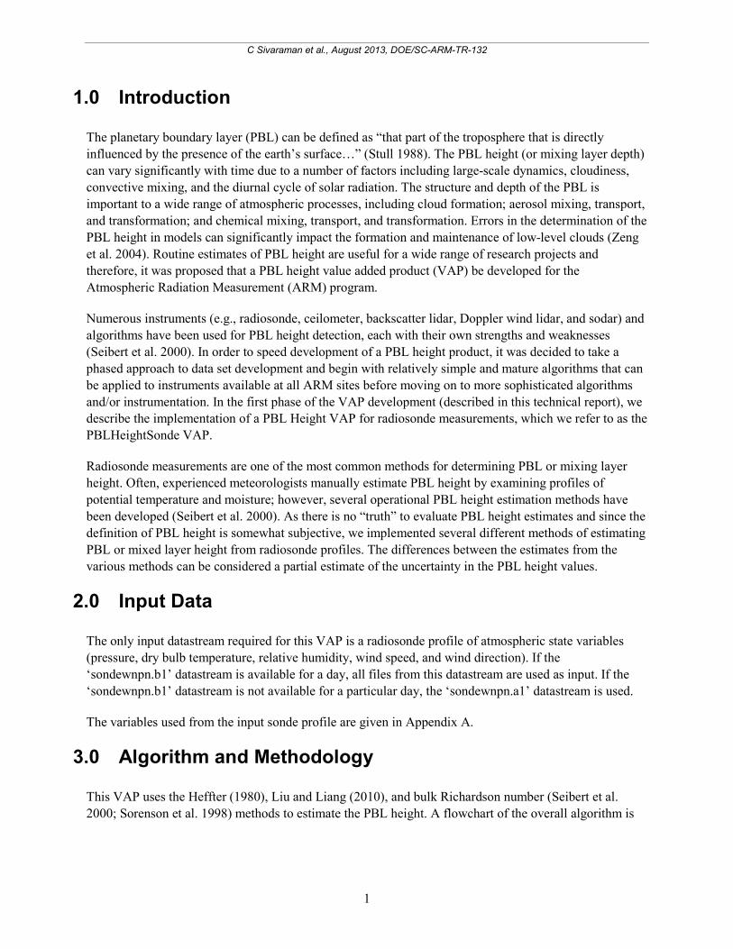
1.0 Introduction

The planetary boundary layer (PBL) can be defined as “that part of the troposphere that is directly influenced by the presence of the earth’s surface…” (Stull 1988). The PBL height (or mixing layer depth) can vary significantly with time due to a number of factors including large-scale dynamics, cloudiness, convective mixing, and the diurnal cycle of solar radiation. The structure and depth of the PBL is important to a wide range of atmospheric processes, including cloud formation; aerosol mixing, transport, and transformation; and chemical mixing, transport, and transformation. Errors in the determination of the PBL height in models can significantly impact the formation and maintenance of low-level clouds (Zeng et al. 2004). Routine estimates of PBL height are useful for a wide range of research projects and therefore, it was proposed that a PBL height value added product (VAP) be developed for the Atmospheric Radiation Measurement (ARM) program.

Numerous instruments (e.g., radiosonde, ceilometer, backscatter lidar, Doppler wind lidar, and sodar) and algorithms have been used for PBL height detection, each with their own strengths and weaknesses (Seibert et al. 2000). In order to speed development of a PBL height product, it was decided to take a phased approach to data set development and begin with relatively simple and mature algorithms that can be applied to instruments available at all ARM sites before moving on to more sophisticated algorithms and/or instrumentation. In the first phase of the VAP development (described in this technical report), we describe the implementation of a PBL Height VAP for radiosonde measurements, which we refer to as the PBLHeightSonde VAP.

Radiosonde measurements are one of the most common methods for determining PBL or mixing layer height. Often, experienced meteorologists manually estimate PBL height by examining profiles of potential temperature and moisture; however, several operational PBL height estimation methods have been developed (Seibert et al. 2000). As there is no “truth” to evaluate PBL height estimates and since the definition of PBL height is somewhat subjective, we implemented several different methods of estimating PBL or mixed layer height from radiosonde profiles. The differences between the estimates from the various methods can be considered a partial estimate of the uncertainty in the PBL height values.

2.0 Input Data

The only input datastream required for this VAP is a radiosonde profile of atmospheric state variables (pressure, dry bulb temperature, relative humidity, wind speed, and wind direction). If the ‘sondewnpn.b1’ datastream is available for a day, all files from this datastream are used as input. If the ‘sondewnpn.b1’ datastream is not available for a particular day, the ‘sondewnpn.a1’ datastream is used.

The variables used from the input sonde profile are given in Appendix A.

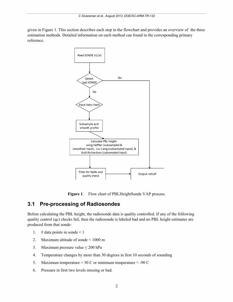
3.0 Algorithm and Methodology

This VAP uses the Heffter (1980), Liu and Liang (2010), and bulk Richardson number (Seibert et al. 2000; Sorenson et al. 1998) methods to estimate the PBL height. A flowchart of the overall algorithm is


2

given in Figure 1. This section describes each step in the flowchart and provides an overview of the three estimation methods. Detailed information on each method can found in the corresponding primary reference.

Figure 1. Flow chart of PBLHeightSonde VAP process.

3.1 Pre-processing of Radiosondes

Before calculating the PBL height, the radiosonde data is quality controlled. If any of the following quality control (qc) checks fail, then the radiosonde is labeled bad and no PBL height estimates are produced from that sonde:

1. # data points in sonde < 1

2. Maximum altitude of sonde < 1000 m

3. Maximum pressure value ≤ 200 hPa

4. Temperature changes by more than 30 degrees in first 10 seconds of sounding

5. Maximum temperature > 50 C or minimum temperature < -90 C

6. Pressure in first two levels missing or bad.


3

After the sonde passes this initial screening, individual sonde data values are checked to be sure they meet valid min/max criteria; failing values are set as missing and qc flags are set (see Section 3.6 for more detail).

Potential temperature, θ, is calculated for each sonde level following the equation:

θ = 𝑇 �𝑝0𝑝�𝑅 𝑐𝑝𝑑�

[Eq 1],

where the reference pressure, p0, is chosen to be 1000 hPa, R is the specific gas constant, and cpd is the specific heat at constant pressure (Curry and Webster 1999). For dry air, R/cpd has a value of 0.286.

To reduce the identification of spurious layers due to noisy data, the radiosonde data is subsampled at 5 mb resolution before the boundary layer height is estimated. A pressure grid is defined at 5 mb intervals from the surface pressure to the top of the radiosonde and output in the daily files with the fieldname, ‘pressure_gridded’. Starting at the surface, the sonde points within each 5 mb interval are identified and the values of pressure, height, potential temperature, wind speed, wind direction, relative humidity, and temperature from the sonde measurement closest to the bottom of the pressure interval are kept. These variables are output in the daily files with fieldnames ‘variable_ss’.

3.2 Determination of Boundary Layer Type

The PBL structure can be classified in three major regimes (Stull 1988; Liu and Lang 2010): the convective boundary layer (CBL), the stable boundary layer (SBL), and a residual layer (RL). The CBL generally occurs in the daytime, is driven by convective thermals, and has strong turbulent mixing. The SBL often forms at night, primarily due to radiative cooling of the surface or warm air advection, and produces a boundary layer that is warmer than the surface, leading to little turbulent mixing. The RL may occur during evening or morning transitions where the existence of the underlying SBL decouples the RL from the surface, but the atmospheric state of the former CBL is maintained.

Following Liu and Liang (2010), we use near-surface potential temperature gradients to identify the boundary layer regime. Residual layers are only identified if they are associated with near-neutral conditions in the surface layer, hence we refer to these as neutral residual layers (NRL). See Liu and Liang (2010) for more details of the definitions of the boundary layer regimes. To identify the regime, the difference in potential temperature (θ) between the fifth and second level of the subsampled soundings is determined and compared to a stability threshold, δs. The following criteria are used to identify the regimes:

θ5–θ2 < -δs = CBL [Eq 2]

θ5–θ2 > +δs = SBL [Eq 3]

-δs ≤ θ5–θ2 ≤ +δs = NRL. [Eq 4]

The values of the stability threshold, δs, vary for land and ocean/ice surfaces and are given in Table 1. In the VAP processing, the value of δs is specified for each site in a configuration file and reported in the output file as a global attribute. The identified regime is reported in variable ‘regime_type’ in the output


4

file, with -1 = CBL, 0 = SBL, and 1 = NRL. The classification of the surface type at each fixed site and at previous ARM Mobile Facility (AMF) deployments is given in Table 2. For future AMF sites, the classification will be made on a case-by-case basis. Currently the island sites (Nauru, Manus, Azores, and Gan) are defined as oceanic sites; further analysis is required to understand if this is appropriate or if island heating drives the PBL depth at these sites.

3.3 Liu-Liang PBL Height Method

Once the boundary layer regime has been identified, we use the criteria defined in Liu and Liang (2010) to estimate the PBL height for each regime.

3.3.1 Convective and Neutral Regimes

For the CBL and NRL regimes, the PBL height is determined as the height at “which an air parcel rising adiabatically from the surface becomes neutrally buoyant.” First, the lowest level, k, that meets the criteria:

𝜃𝑘 – 𝜃1 ≥ 𝛿𝑢 [Eq 5]

is found. In this equation, δu is the potential temperature difference that represents the minimum strength of the unstable layer; it also varies with the surface type (Table 1) and is specified in the configuration file and reported in the output file as global attribute, ‘instability_threshold’.

Once level k is determined, an upward scan is performed to find the lowest level where the potential temperature gradient with height (��𝑘) is greater than 𝜃r , the overshooting threshold of the rising parcel:

��𝑘 ≡ 𝜕𝜃𝑘𝜕𝑧

≥ ��𝑟 [Eq 6]

where ��𝑟 also varies with surface type (Table 1). This level is then considered to be the PBL height for the Liu-Liang method for CBL and NRL regimes. Consistent with Liu and Liang (2010), searches for the criteria given in Equations 5 and 6 use sonde data above 150 m above ground level (AGL) to avoid potentially noisy readings near the surface. If these criteria are not met, i.e., if meteorological conditions are such that a PBL height cannot be determined via this method, then a value of -9999 is reported for the Liu-Liang PBL height.

3.3.2 Stable Regimes

For SBL regimes, the determination of the PBL height is much more uncertain. Turbulence in the SBL can result from either buoyancy forcing or wind shear, and we search for potential layers associated with each.

First, we find the lowest level, k, at which the potential temperature gradient (��𝑘) reaches a minimum and check for the following two conditions:


5

��𝑘 − ��𝑘−1 < −40𝐾/𝑘𝑚

��𝑘+1 < ��𝑟, ��𝑘+2 < ��𝑟 [Eq. 7]

The first condition tests whether the identified level is a local peak with curvature of at least 40 K/km and the second condition tests whether there is an inversion layer in the two layers above the identified layer. If either of the conditions are met, then the height k is the PBL height based on a stability criteria.

Next, we check whether the turbulence generation in the SBL is driven by shear by searching for a low-level jet (LLJ). The nose of the LLJ is defined as the height, j, where the wind speed reaches a maximum, the maximum is at least 2 m/s stronger than the layers immediately above and below, and the wind speed below the maximum decreases monotonically toward the surface. If these criteria are met, then that height, j, is the PBL height based on a wind shear criteria.

If both the stability-derived and wind-shear-derived PBL heights are found, then the PBL height for the SBL regime is defined as the lower of the two heights. If only one height is found, then that height is identified as the PBL height. If no PBL heights are found, then a value of -9999 is reported for the Liu-Liang PBL height.

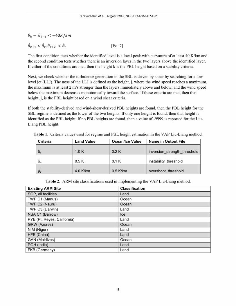
Table 1. Criteria values used for regime and PBL height estimation in the VAP Liu-Liang method.

Criteria Land Value Ocean/Ice Value Name in Output File

δs 1.0 K 0.2 K inversion_strength_threshold

δu 0.5 K 0.1 K instability_threshold

𝜃�� 4.0 K/km 0.5 K/km overshoot_threshold

Table 2. ARM site classifications used in implementing the VAP Liu-Liang method.

Existing ARM Site Classification SGP, all facilities Land TWP C1 (Manus) Ocean TWP C2 (Nauru) Ocean TWP C3 (Darwin) Land NSA C1 (Barrow) Ice PYE (Pt. Reyes, California) Land GRW (Azores) Ocean NIM (Niger) Land HFE (China) Land GAN (Maldives) Ocean PGH (India) Land FKB (Germany) Land


6

3.3.3 Examples

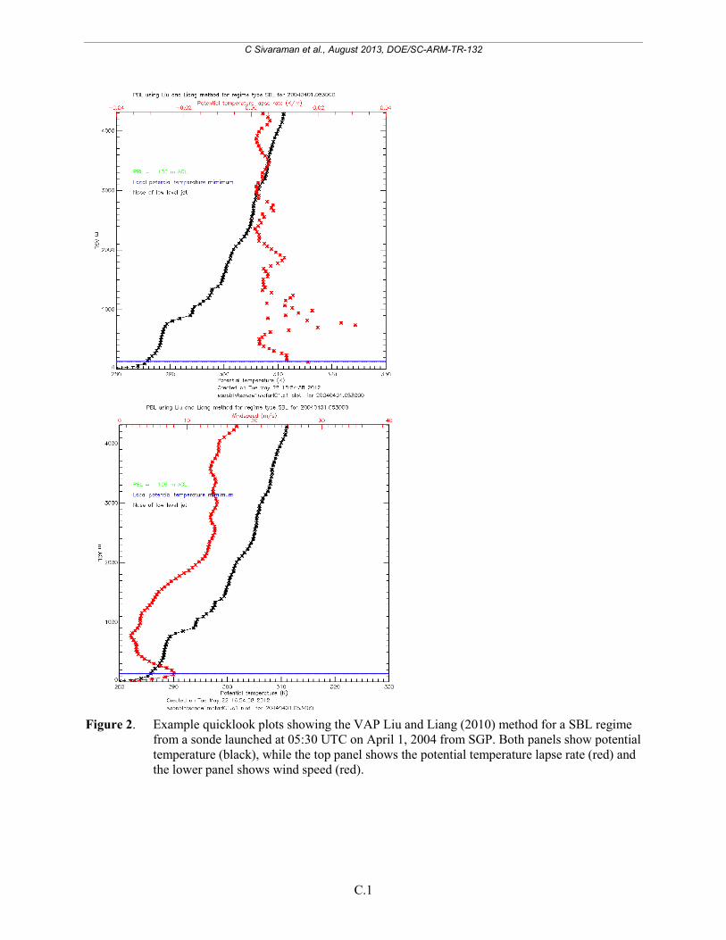
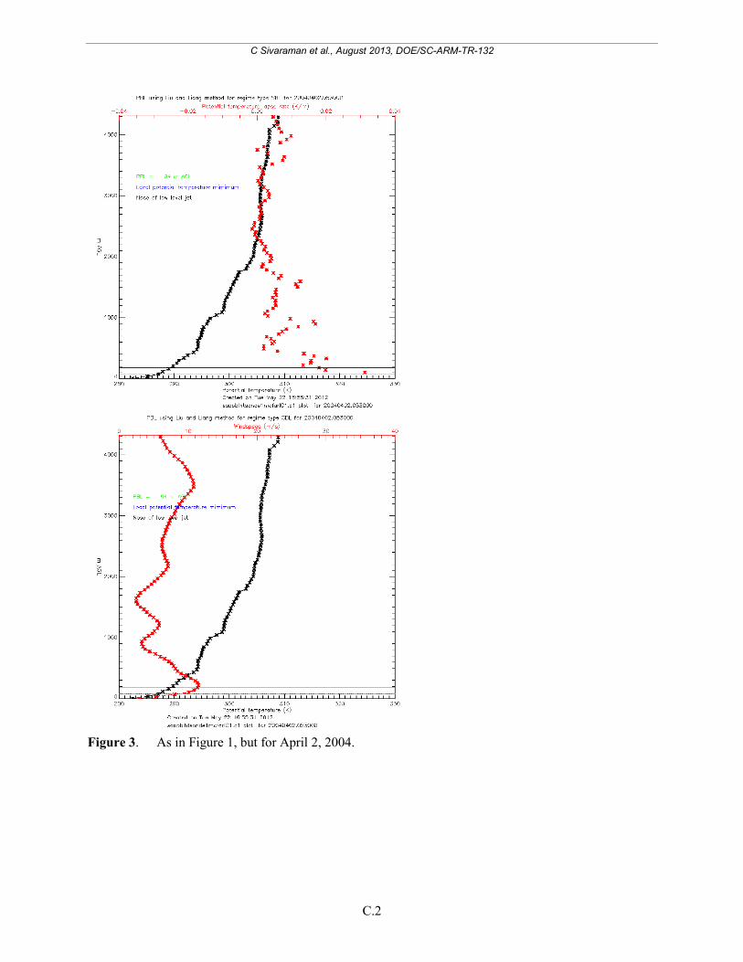
In this section we illustrate the behavior of the Liu-Liang method by showing example quicklooks produced by the VAP. Figures 2 and 3 show quicklooks for two cases classifed as SBL by the Liu-Liang method. In the top panels of each figure, the subsampled potential temperature profile (black) and potential temperature lapse rate (red) are plotted. In the bottom panels, the potential temperature (black) and windspeed (red) profiles are plotted. Additionally, the nose of the LLJ (i.e., the PBL height identified via wind shear criteria), the PBL height identified via stability criteria, and the final PBL height are indicated in each figure. The final PBL height is given in the legend, and the date/time of the sonde and the regime-type are given in the figure heading. In the first case (Figure 2), the stability height (blue line) occurred above the LLJ, so the height of the nose of the LLJ was chosen as the PBL height (green line). In the second case (Figure 3), the nose of the LLJ (black line) is above the stability height, so the stability height was chosen as the PBL height.

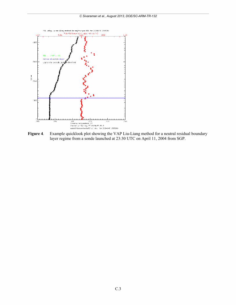
Figure 4 shows an example quicklook for a case classified as NRL by the Liu-Liang method. Here, there is only one panel as the wind speed and LLJ do not enter into the calculations. In this case, the height of the bottom of the unstable layer (blue) and the height where the potential temperature lapse rate exceeds the gradient threshold (black) are both marked, and the latter height is considered to be the PBL height (green).

3.4 Heffter PBL Height Method

The Heffter (1980) method is a well-established and widely used algorithm (e.g., Marsik et al. 1995, Delle Monache et al. 2004, and Snyder and Strawbridge 2004) that determines PBL height from potential temperature gradients using criteria related to the strength of an inversion and the potential temperature difference across the inversion.

To implement the Heffter method, we first perform a three-point moving average to further smooth the subsampled radiosonde data to 15 mb. The smoothing is designed to reduce the number of spurious layers identified because of noise or local variability in the soundings. Next, we identify up to five inversion layers, defined as contiguous heights where the potential temperature lapse rate is greater than 0.005 K/m. The base and top heights of each of these layers, along with the maximum potential temperature lapse rate in the layer, and the maximum potential temperature difference relative to the base of the inversion layer, are all saved in the output file.

We identify the PBL height (‘pbl_height_heffter’) as the lowest inversion layer in which the potential temperature difference between the base and top of the inversion is greater than 2 K. If no layer meets this criteria or if the layer that meets this criteria is > 4 km AGL, then we find the inversion layer with the largest maximum potential temperature gradient and the PBL height is set to the height at which that maximum is reached. In this case, the PBL height is flagged as indeterminate.

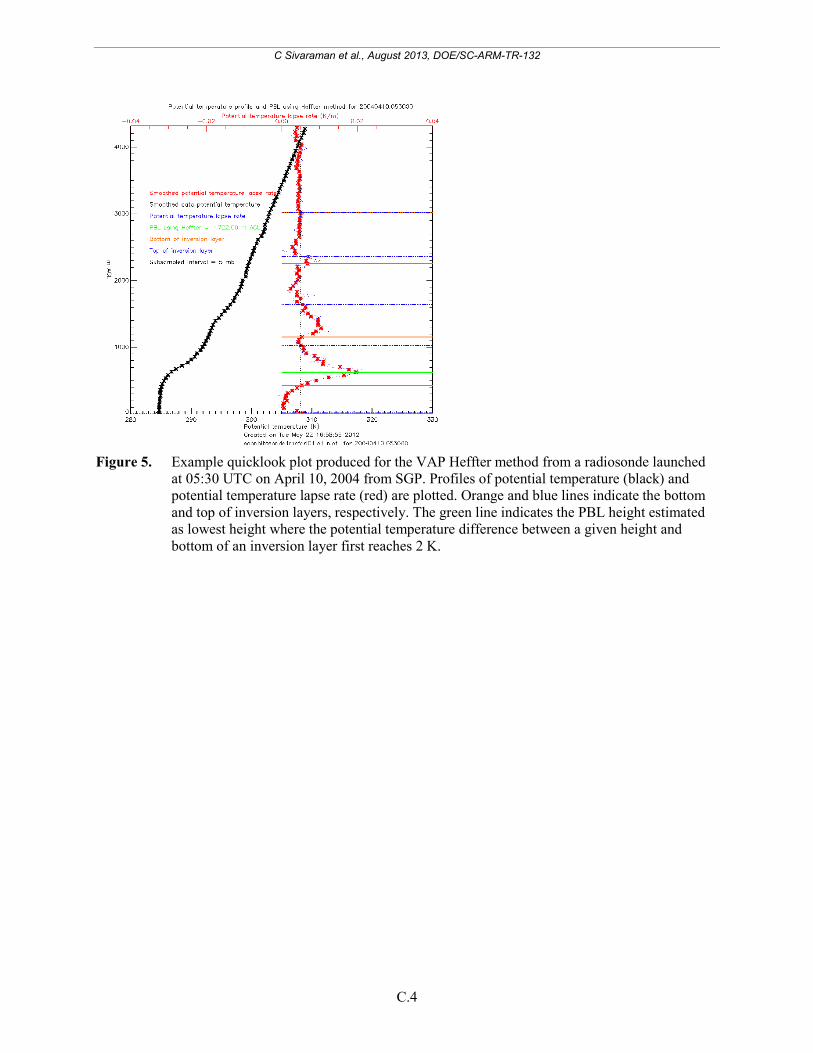
Figure 5 illustrates the Heffter method for a radiosonde launched at 05:30 UTC on April 10, 2004, at the SGP site. The plot shows profiles of potential temperature (black) and potential temperature lapse rate (red). The critical threshold for the potential temperature lapse rate (0.005 K/m) is identified by the vertical dotted black line. The bottom and top heights of each inversion layer exhibiting a lapse rategreater than this threshold are indicated by orange and blue lines, respectively. The green line


7

indicates the PBL height, which is estimated as the lowest height where the potential temperature difference between the given height and the bottom of a critical inversion layer first reaches 2 K.

3.5 Bulk Richardson PBL Height Method

The bulk Richardson number, Rib, is a dimensionless number relating vertical stability to vertical shear. It represents the ratio of thermally produced turbulence to that generated by vertical shear. Methods using Rib to estimate the PBL height assume that there is no turbulence production at the top of the SBL and therefore Ri exceeds its critical value at the top of the boundary layer (Seibert et al. 2000).

Here, following Sorenson et al. (1998), we define the bulk Richardson number at height z AGL as:

𝑅𝑖𝑏 = �𝑔𝑧𝜃𝑣0� �𝜃𝑣𝑧−𝜃𝑣0

𝑢𝑧2+ 𝑣𝑧2� [Eq 8]

where g = acceleration due to gravity; θv0 and θvz are the virtual potential temperature at the surface and height z, respectively; and uz and vz are the wind speed components at height z.

The virtual potential temperature is calculated as:

𝜃𝑣 = 𝑇𝑣 �𝑝0𝑝�𝑅 𝑐𝑝𝑑�

[Eq 9]

Tv is the virtual temperature, given by:

𝑇𝑣 = 𝑇�1 − 𝑒

𝑝(1 − 𝜀)�� [Eq 10]

where ε = 0.622 is the ratio of the molecular weight of water vapor to the molecular weight of dry air and e is the partial pressure of water vapor given by:

e = (RH/100.)*es [Eq 11],

where RH is the relative humidity (in percent) and es is the saturation vapor pressure with respect to liquid water. The saturation vapor pressure is calculated from the equation,

𝑒𝑠 = 𝑒𝑠1exp �− 𝐿𝑙𝑣𝑅𝑣�1𝑇− 1

𝑇1�� [Eq 12]

where Llv is the latent heat of vaporziation, Rv is the gas constant for water vapor, T is the temperature of the air parcel, and es1 and T1 are a reference vapor pressure and temperature, respectively. Accurate calculation of the saturation vapor pressure requires considering the variation of latent heat with temperature. Here, we approximate the saturation vapor pressure assuming the latent heat is constant and using a reference temperature T1 = 273.15 K and reference saturation vapor pressure, es1 = 6.11 hPa.

In the VAP implementation, we use the lowest value in the sonde files to represent the ‘surface’; these are typically the 2 m values from the surface meteorology measurements that are input to the sonde software before the sonde is launched. The PBL height is then chosen as the lowest height at which the value of Rib


8

reaches a critical threshold. The literature suggests several different critical thresholds of the Richardson number, based on resolution of sondes, location, etc. Due to this ambiguity, the VAP includes PBL height estimates based on two critical thresholds: 0.25 and 0.5.

In general, bulk Richardson methods are found to perform best for SBLs with low wind speeds (Siebert et al. 2000). Vogelezang and Holtslag (1996) suggest a modification that includes turbulence produced by surface friction; this modification has not been implemented in the current version of the VAP.

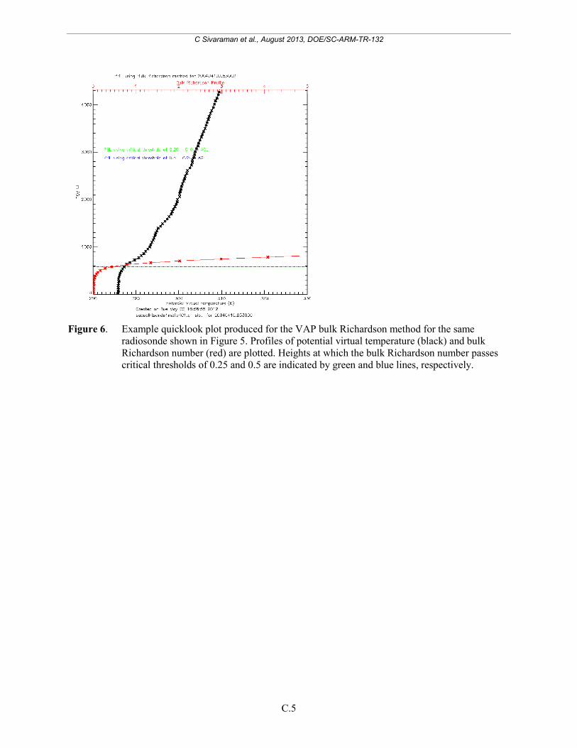
An example of the VAP quicklook for the bulk Richardson method is shown in Figure 6. The profiles of virtual potential temperature (black) and bulk Richardson number (red) are plotted and the heights at which bulk Richardson number passes critical thresholds of 0.25 and 0.5 are indicated by green and blue lines, respectively.

3.6 Quality Control Flags

As described in Section 3.1.1, the initial pre-processing of radiosonde data checks both for situations where an entire sonde data file is considered bad, in which case no PBL height calculations are performed, and situations where individual points within a sonde data file are considered bad and set as missing. In the latter case, PBL height calculations are attempted. At this time we do not fill in or interpolate over bad sonde points; however, we do check for bad or missing values in the input variables. In addition, we check to ensure measured windspeeds near the surface (altitudes < 50 m AGL) are less than 33.5 m/s, and treat the windspeed data in this region as missing if this threshold is exceeded.

Moreover, if the returned PBL height from the Liu-Liang or bulk Richardson methods is greater than 4 km AGL then we flag the PBL height as bad and set it to -9999. For the Heffter method, if the calculated PBL height is greater than 4 km AGL, then the PBL height is set to the strongest inversion layer below 4 km and the QC flag is set to indeterminate. For all methods, if meteorological conditions are such that the governing criteria (e.g., Table 1 values for the Liu-Liang method, critical potential temperature lapse rates and differences for the Heffter method, and critical thresholds for the bulk Richardson number) are not met, then we flag the PBL height as bad and set it to -9999.

4.0 Output Data

There are two processes for this VAP. One process produces the daily output file and the other process reads the daily output files and produces a yearly output file.

The daily output files are named according to the convention

SSSpblhtsonde1mcfarlFF.c1.YYYYMMDD.hhmmss,

where:

SSS = site (e.g., nsa, sgp, twp, pye, etc.)

pblht = VAP class

sonde = instrument used


9

1mcfarl = identifies that this is McFarlane’s version 1 of pblhtsonde

FF = facility (e.g., C1, M1)

YYYYMMDD = year, month, and day

hhmmss = hour, minute, second. (e.g., time of sonde launch)

The yearly output files are named:

SSSpblhtsondeyr1mcfarlFF.c1.YYYYMMDD.hhmmss,

where SSS again specifies the site and YYYYMMDD.hhmmss gives date information for the first day/time in the file.

4.1.1 Output File for Each Sonde

The first set of output files, SSSpblhtsonde1mcfarlFF.c1, consist of a separate detailed file for each sonde launch at a given site and facility and will be produced in near real-time. This file is designed to be used for case studies, applications that need near real-time data, and detailed intercomparisons with other PBL height estimates. The variables included in this file are given in Appendix B. For the detailed file, we output all of the subsampled variables used in the PBL height estimations, the regime-type, and the PBL height estimates from each of the three methods. Furthermore, because determination of the PBL height is somewhat subjective, especially in conditions where residual layers or other complications may exist, we output additional information on preliminary layers identified by the algorithms.

For the Heffter method, we output the base and top heights of up to five identified inversion layers (layers where the potential temperature lapse rate > 5 K/km), along with the maximum potential temperature lapse rate in the layer and the maximum potential temperature difference relative to the base of the inversion layer. For the Liu-Liang method, both the intermediate levels and regime-types are written to output. If the regime-type is CBL or NRL, then level 1 indicates the layer where the potential temperature criteria in Eq 5 is met. If the regime-type is SBL, then level 1 is the local potential temperature minimum. If the regime-type is CBL or NRL, the level 2 height indicates that the lapse rate exceeds the potential temperature gradient threshold. If the regime-type is SBL, the level 2 height indicates the nose of the LLJ. These preliminary layers may be useful to users when comparing to PBL height estimates from other instruments or from model output (Haeffelin et al. 2011).

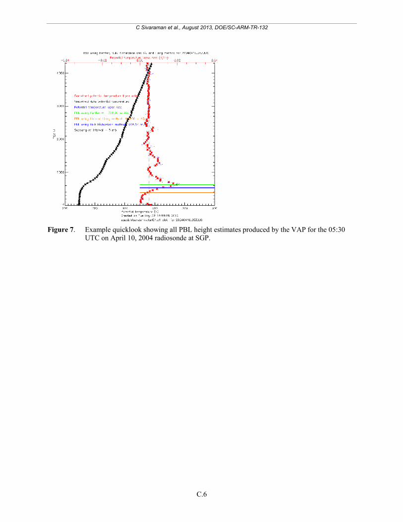
The VAP produces five quicklook plots for each sonde file. Examples of the quicklooks for the individual methods were given in the previous section (Figures 2-6). In addition, a quicklook showing the general overview for each sonde file is produced (Figure 7). The date/time of the sonde are indicated in the heading at the top of the overview plot. The potential temperature is plotted in black, with values given on the lower axis, and the potential temperature lapse rate is plotted in red with values given on the upper axis. The PBL heights from each of the methods are indicated by the horizontal lines and the values for each method are given in the legend.


10

4.1.2 Yearly PBL files

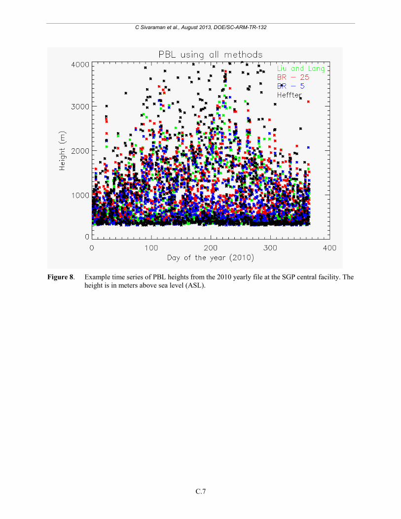
The second type of output file, SSSpblhtsondeyr1mcfarlFF.c1, is designed for the user who is interested in performing long-term analysis or model evaluation of PBL height. This file contains the time series of the PBL height estimates for all sonde launches during the year at the given site. Details of the variables included in this output file are given in Appendix B. This process runs over a year’s worth of daily files, and does not fill in gaps due to missing or failed sonde launches. Figure 8 shows a time series of output from the yearly file at SGP for the year 2010.

5.0 Preliminary Evaluation of PBL Heights

As noted in Section 1.0, the definition of PBL height is somewhat subjective and there is no “truth” to which values produced by the PBLHeightSonde VAP can be readily compared. Detailed evaluations and comparisons of PBL heights from various instrument retrievals (radiosondes, lidars, ceilometers, radar wind profilers, etc.) are planned for the future as other PBL Height VAPs are developed. In the interim, we compare two of the VAP PBL height estimates to independent estimates provided by Dr. Shuyan Liu (University of Maryland) and Dr. Marc Fischer (LBNL), and the four VAP estimates to each other.

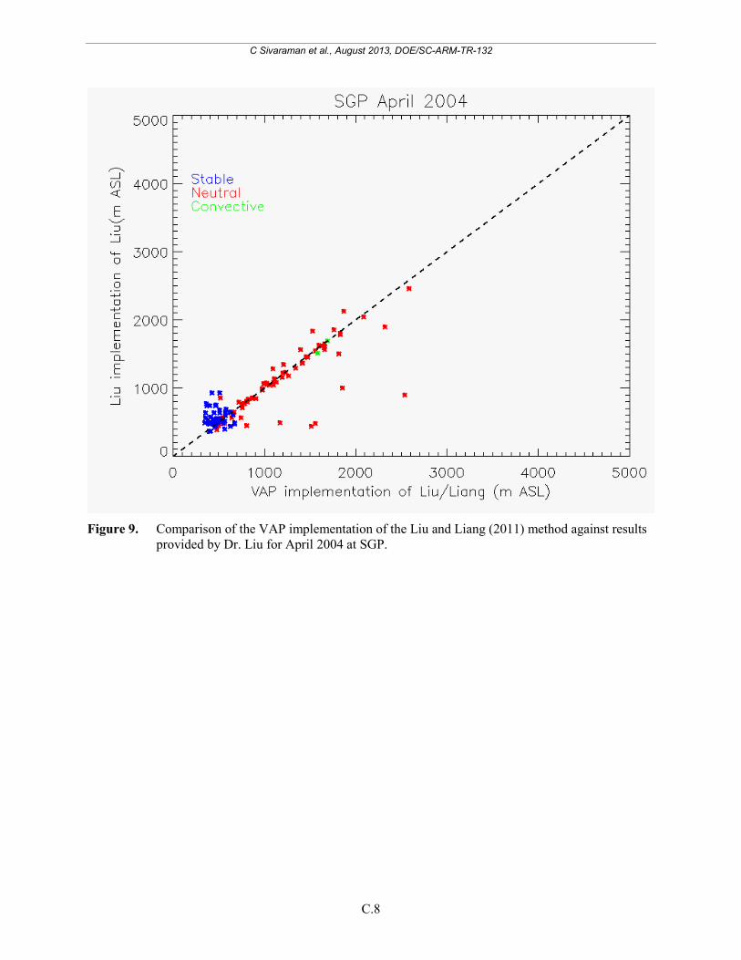
Figure 9 shows the results of the VAP implementation of the Liu and Liang (2010) method against Dr. Liu’s own implementation of the method for radisondes released during the month of April 2004 at the SGP site. The colors represent the different regime-types. In general, there is good agreement with an overall correlation coefficient of 0.86, a mean absolute difference of 137 m, and a median absolute difference of 61 m between the two sets of results. Outlying points with much larger differences do occur, mainly in the SBL regime. Initial analyses indicate differences are likely related to differences in pre-processing and subsampling treatments of the radiosonde data. Further analysis of differences between the two implementations will be conducted as part of future detailed PBL height evaluations.

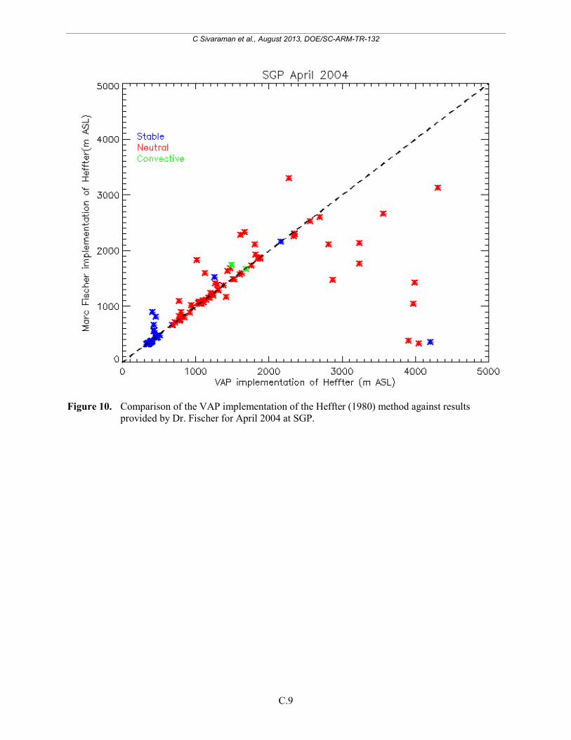
Figure 10 shows the results of the VAP implementation of the Heffter (1980) method against an independent dataset produced by Dr. Fischer, also for the month of April 2004 at the SGP site. Again there is relatively good agreement for the majority of points, with a mean absolute difference of 288 m and a median absolute difference of 29 m. The existence of outliers under both SBL and NRL regimes contributes to an overall correlation coefficient of 0.66. The most extreme outliers occur under neutral conditions (correlation coefficient of 0.44), with the VAP implementation tending to produce higher estimates of PBL height than Dr. Fischer’s implementation. Initial analysis of these cases indicate they typically occur under meteorological conditions with multiple inversion layers; the automated VAP implementation chose a higher inversion layer as the primary PBL height than did the Fischer implementation. Further analysis of these outliers will be conducted as part of future detailed PBL height evaluations.

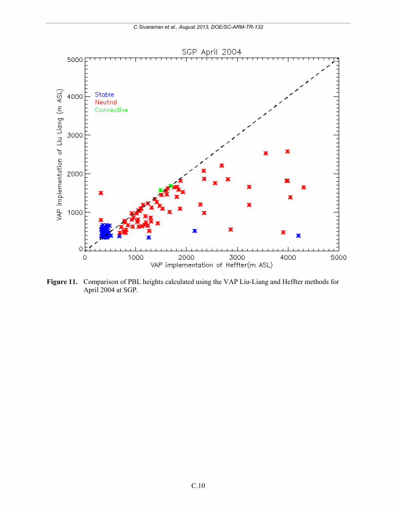
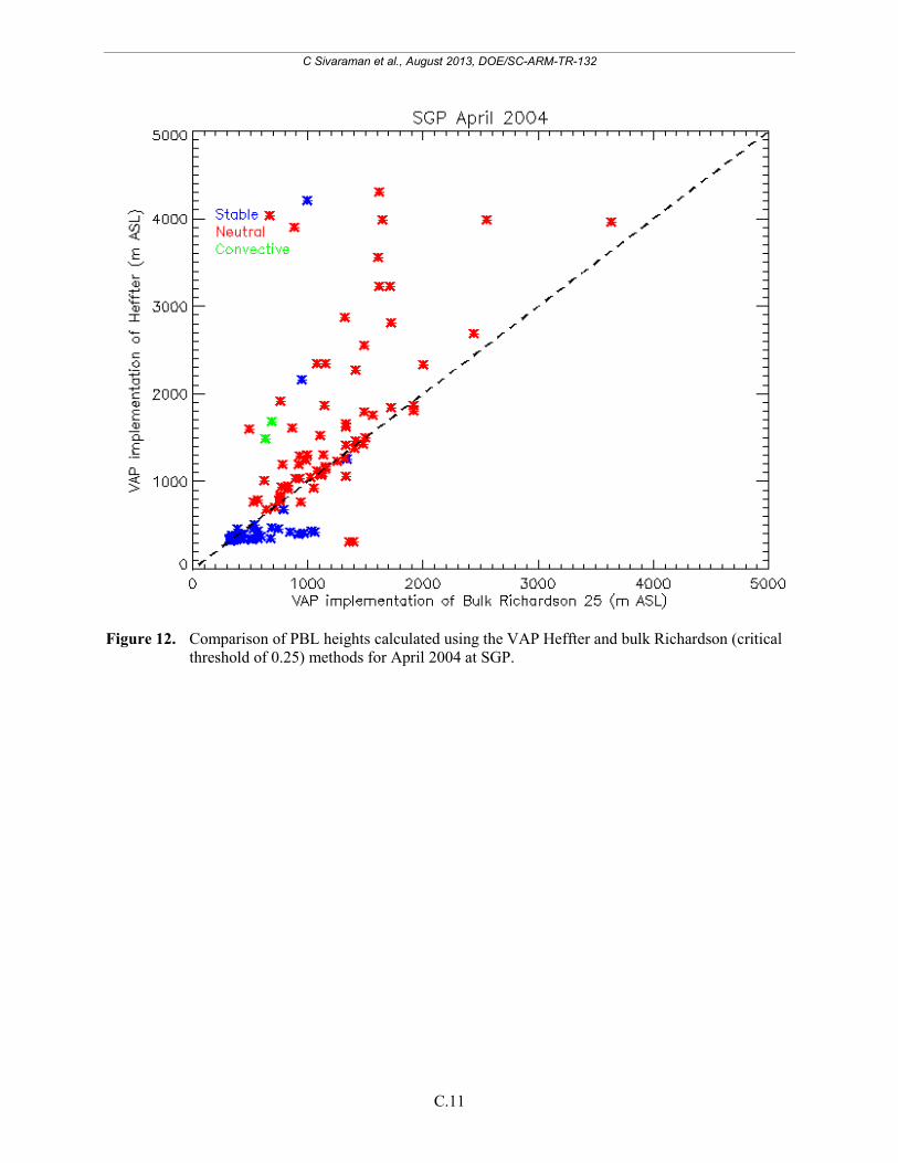
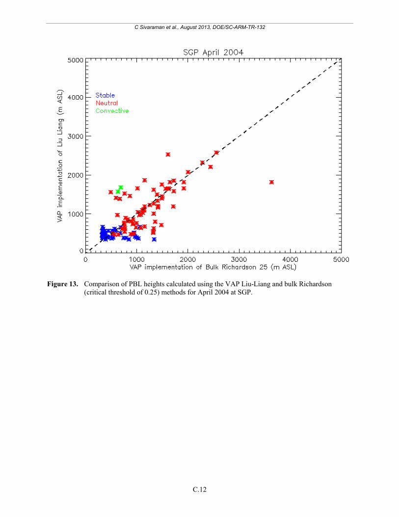
Figures 11-13 summarize the intra-VAP method comparisons, all conducted for the month of April 2004 at the SGP site. As shown in Figure 11, the VAP Heffter method tends to produce higher estimates of PBL height than does the VAP Liu-Liang method. The overall correlation coefficient between these two VAP methods is 0.69, with mean and median absolute differences of 440 m and 185 m. Outliers occur under both the SBL and NRL regimes. The VAP Heffter method also tends to produce higher PBL height estimates than the bulk Richardson method (Figure 12). The overall correlation coefficient between the VAP Heffter and bulk Richardson methods is 0.71, a value similar to the VAP Heffter and Liu-Liang


11

comparison, while mean and median absolute differences are 407 m and 124 m. As shown in Figure 13, the situation is reversed in Liu-Liang and bulk Richardson comparisons, with the bulk Richardson method (critical threshold = 0.25) tending to produce higher PBL height estimates than the VAP Liu-Liang method. The VAP Liu-Liang and bulk Richardson PBL height estimates exhibit an overall correlation coefficient of 0.74 with mean and median absolute differences of 260 m and 133 m. Raising the bulk Richardson critical threshold from 0.25 to 0.50 leads uniformly to higher PBL heights estimated via this method. The higher values do not substantially change the correlation with either the VAP Heffter or Liu-Liang PBL height estimates, raising the overall correlation coefficients only from 0.71 to 0.74 and from 0.74 to 0.76, respectively. The higher estimated PBL heights resulting from the higher bulk Richardson critical threshold lead to changes in mean and median absolute differences with the VAP Heffter estimates (394 m and 165 m, respectively) and the VAP Liu-Liang estimates (302 m and 185 m, respectively).

As other PBL Height VAPs are developed and the planned evaluations and comparisons are conducted, we are hopeful that guidance can be established on which instruments, algorithms, and methodology will produce the most reliable estimate of PBL height under a given set of meteorological conditions at a given geographical location. Until that time, users must expect differences in PBL height estimates produced by the various VAPs, and by the various algorithms within a VAP, using their judgment as to which estimate is most appropriate to employ for their specific application.

6.0 References

Delle Monache L, KD Perry, RT Cederwall, and JA Ogren. 2004. “In situ Aerosol Profiles Over the Southern Great Plains Cloud and Radiation Test Bed Site: 2. Effects of Mixing Height on Aerosol Properties.” Journal of Geophysical Research. 109:D06209. DOI:10.1029/2003JD004024.

Heffter JL. 1980. “Transport Layer Depth Calculations.” Second Joint Conference on Applications of Air Pollution Meteorology, New Orleans, Louisiana.

Liu S and XZ Liang. 2010. “Observed Diurnal Cycle Climatology of Planetary Boundary Layer Height.” Journal of Climate 23:5790–5807.

Marsik FJ, KW Fischer, TD McDonald, and PJ Samson. 1995. “Comparison of Methods for Estimating Mixing Height Used During the 1992 Atlanta Field Intensive.” Journal of Applied Meteorology 34(8):1802–1814.

Seibert P, F Beyrich, SE Gryning, S Joffre, A Rasmussen, and P Tercier. 2000. “Review and Intercomparison of Operational Methods for the Determination of the Mixing Height.” Atmospheric Environment 34(7):1001–1027.

Snyder BJ and KB Strawbridge. 2004. “Meteorological Analysis of the Pacific 2001 Air Quality Field Study.” Atmospheric Environment 38:5733–5743.

Sorensen JH, A Rasmussen, T Ellermann, and E Lyck. 1998. “Mesoscale Influence on Long-range Transport – Evidence From ETEX Modeling and Observations.” Atmospheric Environment, 32(24): 4207–4217.


12

Vogelezang DHP and AAM Holtslag. 1996. “Evolution and Model Impacts of Alternative Boundary Layer Formulations.” Boundary Layer Meteorology 81:245–269.

Zeng X, M Brunke, M Zhou, C Fairall, and N Bond. 2004. “Marine Atmospheric Boundary Layer Height Over the Eastern Pacific: Data Analysis and Model Evaluation.” Journal of Climate 17:4159–4170.


Appendix A


A.1

Table 3. Input Platform and the associated fields.

Platform Names Fields Long Name Sondewnpn.b1 Pres Pressure Rh Relative Humidity wspd Wind Speed tdry Dry Bulb Temperature dp Dewpoint Temperature Deg Wind Direction Alt altitude lat latitude lon longitude Qc_pres Quality check result on field:

Pressure Qc_rh Quality check result on field:

Relative Humidity Qc_wspd Quality check result on field:

Wind Speed Qc_dp Quality check result on field:

Dewpoint Temperature Qc_deg Quality check result on field:

Wind Direction Qc_tdry Quality check result on field:

Dry Bulb Temperature Sondewnpn.a1 Pres Pressure Rh Relative Humidity wspd Wind Direction tdry Dry Bulb Temperature dp Dewpoint Temperature Deg Wind Direction Alt altitude lat latitude lon longitude


Appendix B


B.1

Table 4. Output variables for the daily files.

Variables Long Name base_time Base time in Epoch time_offset Time offset from base time time Time offset from midnight height_ss Height above mean sea level subsampled at 5 mb resolution layer Inversion layer number for Heffter (1980) method atm_pres Atmospheric pressure air_temp Dry bulb ambient air temperature wspd Wind speed rh Relative humidity pbl_height_heffter PBL height above mean sea level calculated using the Heffter (1980) method

qc_pbl_height_heffter Quality check results on field: PBL height above mean sea level calculated using the Heffter (1980) method

pbl_regime_type_liu_liang PBL regime-type determined by Liu and Liang (2010) method qc_pbl_regime_type_liu_liang

Quality check results on field: PBL regime-type determined by Liu and Liang (2010) method

pbl_height_liu_liang PBL height above mean sea level calculated by Liu and Liang (2010) method

qc_pbl_height_liu_liang Quality check results on field: PBL height above mean sea level calculated by Liu and Liang (2010) method

pbl_height_bulk_richardson_pt25

PBL height above mean sea level calculated from bulk Richardson number using critical threshold of 0.25

qc_pbl_height_bulk_richardson_pt25

Quality check results on field: PBL height above mean sea level calculated from bulk Richardson number using critical threshold of 0.25

pbl_height_bulk_richardson_pt5

PBL height above mean sea level calculated from bulk Richardson number using critical threshold of 0.5


Quality check results on field: PBL height above mean sea level calculated from bulk Richardson number using critical threshold of 0.5

pressure_gridded Pressure grid for 5 mb subsampling

lapserate_theta_ss Potential temperature lapse rate subsampled at 5 mb resolution

lapserate_theta_smoothed Potential temperature lapse rate subsampled at 5 mb resolution and then smoothed over 15 mb via three-point moving average

atm_pres_ss Sonde-measured pressure closest to the bottom of the 5 mb subsampling interval

theta_ss Potential temperature subsampled at 5 mb resolution wspd_ss Wind speed subsampled at 5 mb resolution richardson_number Bulk Richardson number virtual_theta_ss Virtual potential temperature

bottom_inversion Height above mean sea level at bottom of inversion layer from Heffter (1980) method

top_inversion Height above mean sea level at top of inversion layer from Heffter (1980) method

lapserate_max Maximum lapse rate in inversion layer from Heffter (1980) method

delta_theta_max The maximum difference in potential temperature across inversion layers from Heffter (1980) method

level_1_liu_liang Level 1 height above mean sea level calculated by the Liu and Liang (2010) method

level_2_liu_liang Level 2 height above mean sea level calculated by the Liu and Liang (2010) method


B.2

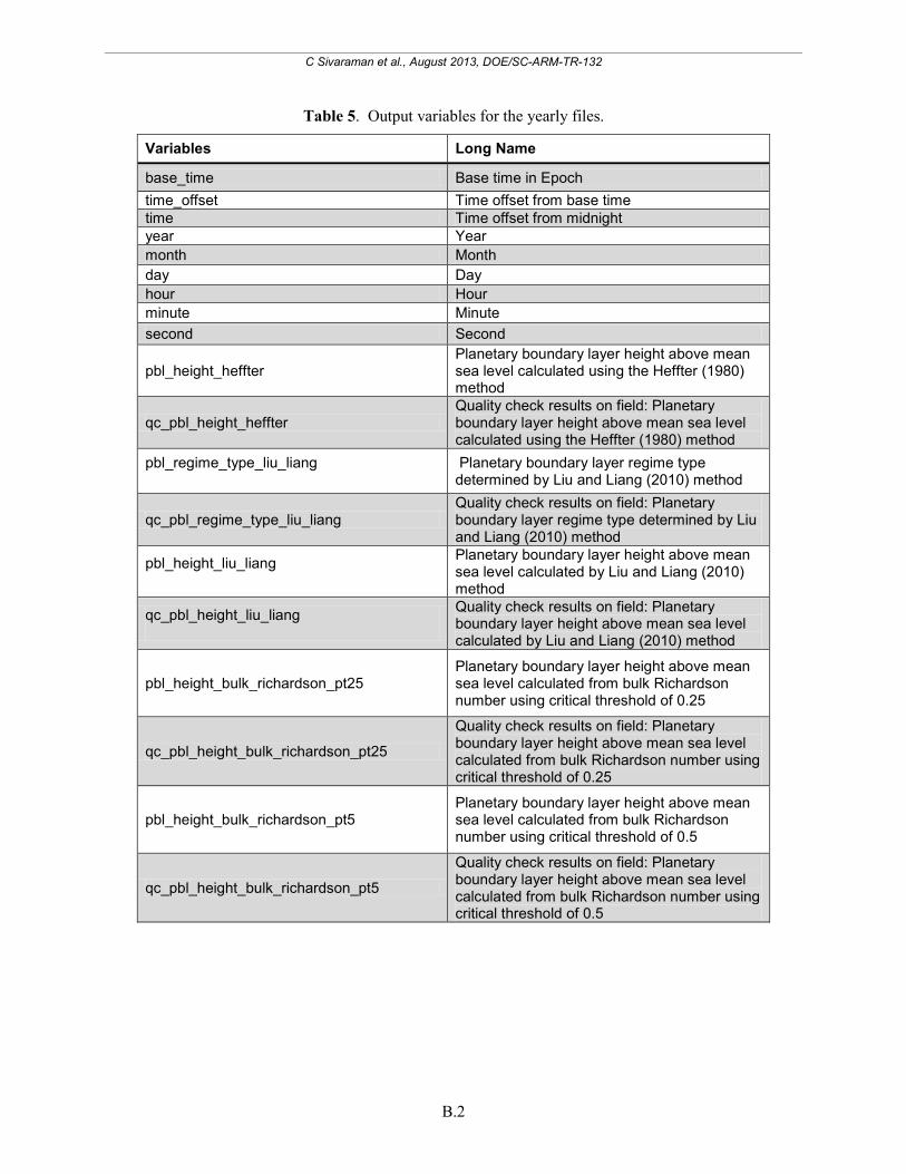
Table 5. Output variables for the yearly files.

Variables Long Name

base_time Base time in Epoch time_offset Time offset from base time time Time offset from midnight year Year month Month day Day hour Hour minute Minute second Second

pbl_height_heffter Planetary boundary layer height above mean sea level calculated using the Heffter (1980) method

qc_pbl_height_heffter Quality check results on field: Planetary boundary layer height above mean sea level calculated using the Heffter (1980) method

pbl_regime_type_liu_liang

Planetary boundary layer regime type determined by Liu and Liang (2010) method

qc_pbl_regime_type_liu_liang Quality check results on field: Planetary boundary layer regime type determined by Liu and Liang (2010) method

pbl_height_liu_liang

Planetary boundary layer height above mean sea level calculated by Liu and Liang (2010) method

qc_pbl_height_liu_liang

Quality check results on field: Planetary boundary layer height above mean sea level calculated by Liu and Liang (2010) method

pbl_height_bulk_richardson_pt25 Planetary boundary layer height above mean sea level calculated from bulk Richardson number using critical threshold of 0.25


Quality check results on field: Planetary boundary layer height above mean sea level calculated from bulk Richardson number using critical threshold of 0.25

pbl_height_bulk_richardson_pt5 Planetary boundary layer height above mean sea level calculated from bulk Richardson number using critical threshold of 0.5


Quality check results on field: Planetary boundary layer height above mean sea level calculated from bulk Richardson number using critical threshold of 0.5


Appendix C Figures


C.1

Figure 2. Example quicklook plots showing the VAP Liu and Liang (2010) method for a SBL regime

from a sonde launched at 05:30 UTC on April 1, 2004 from SGP. Both panels show potential temperature (black), while the top panel shows the potential temperature lapse rate (red) and the lower panel shows wind speed (red).


C.2

Figure 3. As in Figure 1, but for April 2, 2004.


C.3

Figure 4. Example quicklook plot showing the VAP Liu-Liang method for a neutral residual boundary

layer regime from a sonde launched at 23:30 UTC on April 11, 2004 from SGP.


C.4

Figure 5. Example quicklook plot produced for the VAP Heffter method from a radiosonde launched

at 05:30 UTC on April 10, 2004 from SGP. Profiles of potential temperature (black) and potential temperature lapse rate (red) are plotted. Orange and blue lines indicate the bottom and top of inversion layers, respectively. The green line indicates the PBL height estimated as lowest height where the potential temperature difference between a given height and bottom of an inversion layer first reaches 2 K.


C.5

Figure 6. Example quicklook plot produced for the VAP bulk Richardson method for the same

radiosonde shown in Figure 5. Profiles of potential virtual temperature (black) and bulk Richardson number (red) are plotted. Heights at which the bulk Richardson number passes critical thresholds of 0.25 and 0.5 are indicated by green and blue lines, respectively.


C.6

Figure 7. Example quicklook showing all PBL height estimates produced by the VAP for the 05:30

UTC on April 10, 2004 radiosonde at SGP.


C.7

Figure 8. Example time series of PBL heights from the 2010 yearly file at the SGP central facility. The

height is in meters above sea level (ASL).


C.8

Figure 9. Comparison of the VAP implementation of the Liu and Liang (2011) method against results

provided by Dr. Liu for April 2004 at SGP.


C.9

Figure 10. Comparison of the VAP implementation of the Heffter (1980) method against results

provided by Dr. Fischer for April 2004 at SGP.


C.10

Figure 11. Comparison of PBL heights calculated using the VAP Liu-Liang and Heffter methods for

April 2004 at SGP.


C.11

Figure 12. Comparison of PBL heights calculated using the VAP Heffter and bulk Richardson (critical

threshold of 0.25) methods for April 2004 at SGP.


C.12

Figure 13. Comparison of PBL heights calculated using the VAP Liu-Liang and bulk Richardson

(critical threshold of 0.25) methods for April 2004 at SGP.

Documents

Planetary Boundary Layer (PBL) Height Value Added … Boundary Layer (PBL) Height Value Added Product (VAP): Radiosonde Retrievals ... (or mixing layer depth)