Embed Size (px)
Citation preview
PLANNING AND ENVIRONMENTAL POLICY
RESEARCH SERIES
WORKING PAPERS
2006
Happiness, Geography and the Environment
Finbarr Brereton, J. Peter Clinch, and Susana Ferre ira
University College Dublin
PEP 06/04
Planning and Environmental Policy
University College Dublin
www.ucd.ie/pepweb
PLANNING AND ENVIRONMENTAL POLICY∗∗∗∗
RESEARCH SERIES
WORKING PAPERS
2006
Happiness, Geography and the Environment Brereton, Clinch and Ferreira
PEP 06/04 University College Dublin 1
Happiness, Geography and the Environment
Finbarr Brereton, J. Peter Clinch, and Susana Ferre ira
University College Dublin
PEP/06/04
ISSN 1649-5586
July 06
© Finbarr Brereton, J. Peter Clinch, and Susana Fer reira (2006)
PLANNING AND ENVIRONMENTAL POLICY,
UNIVERSITY COLLEGE DUBLIN,
RICHVIEW, CLONSKEAGH,
DUBLIN 14, IRELAND
Happiness, Geography and the Environment
Finbarr Brereton, J. Peter Clinch, and Susana Ferre ira1
Planning and Environmental Policy
University College Dublin
∗ Formerly: Environmental Studies Research Series (ESRS) 1 We thank Andrew Oswald, Michael Hanemann, Mirko Moro and Alan Carr for fruitful discussions. We thank Daniel McInerney and Sean Morrish for technical assistance. The usual disclaimer applies.. Financial support of the Environmental Protection Agency ERTDI program is gratefully acknowledged. The usual disclaimer applies.
Happiness, Geography and the Environment Brereton, Clinch and Ferreira
PEP 06/04 University College Dublin 2
Abstract
In recent years, economists have being using socio-economic and socio-demographic characteristics to explain self-reported individual happiness or satisfaction with life. Using Geographical Information Systems (GIS), we employ data disaggregated at the individual and local level to show that while these variables are important, consideration of amenities such as climate, environmental and urban conditions is critical when analyzing subjective well-being. Location-specific factors are shown to have a direct impact on life satisfaction. Most importantly, however, the explanatory power of our happiness function substantially increases when the spatial variables are included, highlighting the importance of the role of the spatial dimension in determining well-being. This may have potentially important implications for setting priorities for public policy as, in essence, improving well-being could be considered to be the ultimate goal of public policy.
Keywords: subjective well-being; spatial amenities; geography; environment; Geographical
Information Systems.
Correspondence to: Peter Clinch, Planning and Environmental Policy, University College Dublin, Richview, Clonskeagh, Dublin 14, Ireland. Tel: +353-1-716 2571; Fax: +353-1-716 2788; E-mail: [email protected] Citation: Brereton, F. Clinch, J.P. and Ferreira, S. (2006). “Happiness, Geography and the Environment”, Planning and Environmental Policy Research Series (PEP) Working Paper 06/04, Planning and Environmental Policy, University College Dublin.
Happiness, Geography and the Environment Brereton, Clinch and Ferreira
PEP 06/04 University College Dublin 3
I. Introduction
The economics of happiness literature developed in the early nineteen seventies with the
pioneering work of such researchers as Richard Easterlin. Easterlin and subsequent authors,
such as Daniel Kahneman, believe that individual utility, traditionally thought by economists to
be immeasurable and hence proxied by income, can be measured directly. One method is to
employ happiness data from surveys as empirical approximations of individual utility. The
specific question asked varies throughout the literature in terms of subject matter (questions
on happiness and life satisfaction are frequently employed) and range of scale (three-point to
ten-point scales have been employed in the literature). These questions elicit happiness or life
satisfaction from individuals and measures such as these have been found to have a high
scientific standard in terms of internal consistency, reliability and validity (Diener et al., 1999)2
and have been used extensively in the economics literature in recent decades (see, e.g.,
Easterlin, 1974; 1995; 2001, or Frey and Stutzer, 2000; 2002a; 2002b; 2004).
This literature has examined the role of socio-economic and socio-demographic variables on
individual well-being. Established findings within the field include that characteristics of the
individual’s themselves i.e., their socio-demographic characteristics, such as their age,
gender and marital status, influence their happiness. Similarly for micro-economic
characteristics, such as income, household tenure and employment status, with
unemployment having a profound negative influence on well-being. At the macro-economic
level, contributions have focused on the impact of national inflation (Di Tella et al., 2001) and
unemployment (Clark and Oswald, 1994) rates and also the type of governance present in the
person’s area (Frey and Stutzer, 2000). Happiness is found to be inversely related to the
inflation and unemployment rates, but to increase with the level of direct democracy.
Prior literature in the economics field has demonstrated that the area or location where an
individual lives affects quality of life. This is especially evident in the hedonic pricing literature
where there is a long tradition of constructing quality of life indices as the weighted averages
of amenities in a particular area, usually a city region (see Rosen, 1974; Roback, 1982 or
Blomquist, et al., 1988, for seminal contributions, and Chay and Greenstone, 2005, for a
recent state-of-the-art valuation exercise).3
2 Firstly, measures of life satisfaction show temporal reliability, even over a period of several years; secondly, they covary with ratings made by family and friends, with interviewer ratings and with amount of smiling in an interview; and finally, when self-reports of well-being are correlated with other methods of measurement, they show adequate convergent validity (Diener and Suh, 1999). 3 Roback (1982) found that the average person in her sample would be willing to pay $69.55 per year for an additional clear day, $78.25 per year to avoid an additional cloudy day, and $5.55 per year to avoid an increase of 1 microgram per cubic meter in particulate matter. Blomquist et al. (1988) found that the difference in compensation between the most and least desirable U.S. counties in terms of the same bundle of local amenities comprising climate, urban conditions and environmental quality was $5,146. More recently, Berger et al. (2003) have shown that one standard deviation changes in climate attributes (heating degree days), air quality and crime produce annual compensation in the Russian housing and labor markets of 7,839, 8,050 and 8,602 rubles respectively, compared to a mean monthly salary of 1,928 rubles.
Happiness, Geography and the Environment Brereton, Clinch and Ferreira
PEP 06/04 University College Dublin 4
However, it wasn’t until the 1990s that researchers began to examine this spatial aspect of
well-being in the economic psychology literature. These more recent papers found that
characteristics of people’s immediate surroundings (their locality) influenced their well-being,
but also that the wider environment had an important role to play in explaining what makes us
happy. Environmental variables such as aircraft noise (Van Praag and Baarsma, 2005), air
pollution (Welsch, 2006) and the prevailing climate (Frijters and Van Praag, 1998 and
Rehdanz and Maddison, 2005) are found to influence welfare, as are environmental attitudes
(Ferrer-i-Carbonell and Gowdy, 2007). Findings indicate that excess noise levels adversely
affect well-being, as does air pollution and the influence of climate depends on the variable in
question, indicating the potential importance of spatial factors in determining well-being.
In terms of examining the geography of well-being, previous studies were hindered by a lack
of adequately disaggregrated data (Welsch, 2006; Rehdanz and Maddison, 2002). By the
authors own admission, data constraints at the local and regional levels restricted their
analysis to aggregated data at the national level, or to focusing on a particular localised area
where richer data was available. Hence, thus far, the current literature has stopped short of
carrying out a holistic study of the spatial element of well-being, due in no small part to these
data constrains, but also to the lack of availability of appropriate tools to carry out such
analysis. For example, Rehdanz and Maddison (2005) examine the influence on well-being of
climatic conditions, but including too many of their climate variables in the model at once
leads to problems of multicollinearity as some of their climate variables did not vary at the
national level (i.e., one record per country). They state that their analysis was restricted to the
country level and that it would be interesting to see how climate would affect people’s
happiness in different regions of a country. Ferrer-i-Carbonell and Gowdy (2007) include a set
of dummy variables indicating the region where the individual lives to capture the (natural)
environment, proxying, for example, London and Manchester as polluted areas. However, in
the case of major cities in developed countries, pollution is, generally, a localised
phenomenon and categorising an entire cities population under one pollution level may
severely under or overestimate their exposure. Welsch (2006) uses life satisfaction scores to
value air pollution in European countries, but includes no within country variation in his
estimation. Due to a lack of data, Welsch’s study was concerned with countries as the cross-
sectional units and he states that “future research may address the question how regional or
local happiness profiles are affected by the corresponding environmental conditions. It is
conceivable that at a more disaggregated level the linkage between environment and
happiness is even more articulate than it is with respect to national data”. Van Praag and
Baarsma (2005) examine a localised problem and use postcodes to link their respondents to
objective noise burden, but due to issues of anonymity, this application may only be available
at city level where populations are aggregated.
Happiness, Geography and the Environment Brereton, Clinch and Ferreira
PEP 06/04 University College Dublin 5
In this paper, we explicitly endeavour to examine the importance of space in the
determination of well-being, using a more holistic approach. Firstly, we measure amenities at
the level of disaggregation at which individuals actually experience their surroundings, i.e.
local level. This is facilitated through the use of Geographical Information Systems (GIS), a
system for the visual display of spatial data. Using GIS, 1) the level of disaggregation at which
individuals are linked to their surroundings is greatly improved; 2) the vector of spatial
variables included in the happiness function is expanded to include variables with a potential
influence on well-being, but which have not been examined to date; and 3) distance
measures are introduced, as one could hypothesis that the intensity at which individuals
experience their surroundings is a function of proximity (as in the case of air pollution and
noise). The findings in the paper highlight the critical importance of the role of the spatial
dimension in determining well-being, i.e., spatial variables are found to be highly significant
with large coefficients. We also find that the impact of spatial amenities on life satisfaction is a
function of distance, with the most notable example being that of proximity to coast. This has
a large positive effect, which diminishes as one moves further from the coast. Most
importantly, the explanatory power of our happiness function substantially increases when the
spatial variables are included, resulting in three-times the variation in well-being being
explained than has been achieved in any previous cross-sectional study. This indicates that
geography and the environment have a much larger influence on well-being than previously
thought.
The paper proceeds as follows. Section 2 describes the methodology (data, GIS requirements
and the estimation strategy) used in the paper, section 3 presents the results and section 4
concludes.
II. Methodology
In this paper, we assume that the level of well-being attained by an individual i in location k
can be represented by the following indirect utility function:
(1) kikikikiu ,,,, '' εγβα +++= ax Ii ....1= , k = 1,…,K
where u denotes utility of individual i in location k, a is a vector of spatial factors, some of
which (e.g., commuting time, proximity to a coast) may vary at an individual level and x is a
vector of socio-economic and demographic characteristics (age, gender etc.) that are typically
included in the literature (see, e.g., Clark and Oswald, 1994; Di Tella et al., 2001 or Stutzer,
2004). In the micro-econometric function, the individual’s true utility is unobservable, hence
we use self-reported well-being as a proxy.
Happiness, Geography and the Environment Brereton, Clinch and Ferreira
PEP 06/04 University College Dublin 6
The well-being indicator (or proxy for individual utility) used in this paper is based on the
answers to the following question (which was preceded by a range of questions regarding
various aspects of the respondent’s life): ‘Thinking about the good and bad things in your life,
which of these answers best describes your life as a whole?’. Respondents could choose a
category on a scale of one to seven (‘As bad as can be’; ‘very bad’; ‘bad’; ‘alright’; ‘good’;
‘very good’; ‘as good as can be’).4 The use of self-reported well-being introduces
measurement error as the respondents may be unable to communicate accurately their
underlying utility level. However, as Blanchflower and Oswald (2004a) point out, it is
measurement error in the independent variables that would be more problematic in the
econometric estimation, and there is a broad consensus among previous studies that self-
reported well-being is a satisfactory empirical proxy of individual utility (see, e.g., Stutzer,
2004; Blanchflower and Oswald, 2004b; Ferrer-i-Carbonell and Frijters, 2004).
Data on well-being and on the socio-demographic and socio-economic characteristics used in
the analysis come from a survey5 of a representative sample of 1,5006 men and women, aged
18 and over and living in Ireland. The survey found a high well-being, in general, in Ireland
with an average of 5.5 on the seven-point scale. What makes this data set particularly well
suited for this paper is that it can be merged with detailed geographical information as we
know the area in which the respondent lives. This information allows us to match the survey
data spatially to a national map of Ireland using GIS (Appendix I) and hence it is possible to
combine subjective data at the individual level with a vector of spatial amenities (a).7 These
two datasets are combined at the local (electoral division8) level. However, to assess properly
the impact on individual well-being from changes in spatial amenities, ideally, one would want
to be able to match climate and environmental factors to a particular individual rather than a
particular area. At present, however, the data do not allow this and anonymity may preclude
this in any case. Descriptions of the variables and descriptive statistics are outlined in
Appendix II.
4 Some studies treat self-reported life satisfaction data and happiness data interchangeably. Veenhoven (1997) states that “the word life-satisfaction denotes the same meaning and is often used interchangeably with happiness.” Di Tella et al. (2001) report a correlation coefficient of 0.56. However, Peiro (2006) points to happiness and satisfaction as two distinct spheres of well-being. He concludes that the first would be relatively independent of economic factors while the second would be strongly dependent. 5 Urban Institute Ireland National Survey on Quality of Life (2001)
6 Due to missing observations the final sample consists of approximately (depending on the model specification) 1,467 observations. The effective response rate is 66.6 percent. The margin of error using the entire sample is ± 2.5 percent at a 95 percent confidence level. The 2000 Register of Electors was used as the sampling frame. 7 GIS works well when applied to static data, and less well when applied to time series analysis (Goodchild and Haining, 2004) and hence is well-suited to the cross-sectional data employed in this paper.
8 There are around 3440 electoral divisions in Ireland which represent the smallest enumeration area used by the Irish Central Statistics Office in the collection of Census data. These areas are relatively small, particularly in the city regions and those represented in our sample range in size from 18 hectares (in cities) to 6189 hectares (open countryside) (mean = 1767, standard deviation = 1538), with total populations ranging from 47 individuals to 8595 (mean = 2040, standard deviation = 2073).
Happiness, Geography and the Environment Brereton, Clinch and Ferreira
PEP 06/04 University College Dublin 7
The use of data collected in Ireland is interesting in its own right. In the last decade, the ‘Celtic
Tiger’ economy grew at a record rate for a developed country (this and other trends are
documented in, for example, Clinch et al., 2002). Meanwhile, the Economist Intelligence Unit
(2004) has ranked Ireland as first in its quality of life league table for 2005. Nevertheless,
there has been much concern regarding the implications of the pace of economic growth for
localized environmental quality and life satisfaction generally (EPA, 2004a). This makes
Ireland an appropriate subject for the analysis of the influence of spatial amenities on
subjective well-being. Furthermore, issues surrounding heterogeneity of preferences may not
be as problematic in a small (approximately 70,000 km2) and relatively homogenous country
like Ireland, compared to other nations. Also, by examining one country, issues of translation
and cultural bias in the well-being question should not arise.9
As elements of the vector of spatial factors, the dataset contains climate (from Collins and
Cummins, 1996), environmental (from EPA, 2005) and other spatial data (UII, 2006). Several
climate variables were considered but following the advice of a climatologist, mean annual
precipitation, January mean daily minimum air temperature, July mean daily maximum air
temperature, mean annual duration of bright sunshine and mean annual wind speed were
chosen (similar to those included in Frijters and van Praag, 1998).
As in Blomquist et al. (1988), variables capturing whether the respondent lives near the coast,
the violent crime rate and presence of waste facilities in the respondent’s area were included.
There is evidence suggesting that noise, smell and other negative externalities from waste
facilities may impact negatively on well-being or quality of life (DG Environment, 2000). Air
pollution and water quality were considered as indicators of environmental quality but regional
variation is minimal (EPA, 2004). Additionally, population density (total population divided by
total area in km2 (CSO, 2003)), traffic congestion and average commuting time in each area
were included to capture crowding and congestion effects. Also, a variable capturing voter
turnout in the Irish general election in 2002 (Kavanagh, Mills and Sinnott, 2004) is included as
an indicator for social capital (as in Putnam, 2000). Due to data constraints, traffic congestion
(number of vehicles (DELG, 2002a) divided by the total length of primary roads per local
authority10 area (NRA, 2003)) and the homicide rate (number of homicides per 100,000 of
population (Garda Siochana, 2002)) are measured at the local authority level.
9 However, the extent to which these biases are problematic is a matter of debate (Diener and Suh, 1999) 10 For governance purposes, Ireland is divided into 34 different regions called Local Authority areas. These generally equate to one body per county and one for the three major urban areas of Galway City, Limerick City and Cork City. Dublin is divided into four areas and Tipperary is divided into two local authority areas. These areas are relatively large and range in size from 2035 hectares to 746797 hectares (mean = 229060, standard deviation = 226508), with total populations ranging from 25799 individuals to 495781 (mean = 177377, standard deviation = 135990).
Happiness, Geography and the Environment Brereton, Clinch and Ferreira
PEP 06/04 University College Dublin 8
As in van Praag and Baarsma (2005), we include proximity to airports.11 However, we also
include more detailed transport data consisting of proximity to: major roads (national primary
and national secondary) (NRA, 2003); international, national and regional airports; railway
stations and seaports (UII, 2003). Access to transport routes could potentially enter the micro-
econometric function in two ways, positively through accessibility and negatively through
pollution and noise. The latter was shown to be the case by van Praag and Baarsma (2005) in
relation to airport noise in Amsterdam.
As for the socio-economic and demographic variables, the dataset includes an employment-
status variable divided into ten separate categories which follow the International Labour
Organisation (ILO) classification: employed (self-employed, full-time employed and part-time
employed), inactive (student, working on home duties, disabled, retired, those not working
and not seeking work, and those on a government training scheme) or unemployed (CSO,
2006). Unemployment is further divided into two categories of those unemployed having lost
or given up their job combined with those not working but seeking work, and those seeking
work for the first time. Additional individual characteristics contained in the dataset and
typically employed in the literature are age, gender, educational attainment (primary, lower
secondary/junior high school, upper secondary/senior high school and university degree),
marital status (single, married, cohabiting, widowed and separated/divorced), log of gross
household income,12 whether the respondent is caring for a disabled member of the family
and the number of dependent children in the household (1, 2, 3+). As an indicator of individual
health we use the number of times the respondent has visited the doctor in the past year
(never or once, two to five times and six or more times a year). We also include household
tenure (owned outright, mortgaged, renting, or in public housing).
II.I. Geographical Information Systems Methodology
GIS is a powerful computing tool that allows the visual representation of spatially referenced
data. It has advanced the technical ability to handle such data as countable numbers of
points, lines and polygons13 in two-dimensional space (Goodchild and Haining, 2004) and link
various datasets using spatial identifiers (Bond and Devine, 1991). It represents a solid base
for spatial data analysis and provides a range of techniques for analysis and visualisation of
spatial data. It provides effective decision support through its database management
capabilities, graphical user interfaces and cartographic visualisation (Wu et al., 2001).
11 All the proximity criteria are based on guidelines in Irish Government policy documents (see, DELG, 2002b). 12 Income is expressed in thousands of euro. Missing values, 23.7 percent of those interviewed, were imputed based on the respondent’s socio-demographic characteristics including age, gender, marital status, education level, area inhabited and employment status. The original income variable was divided in 10 categories, so mid-points were used (as in Stutzer, 2004). The survey was carried out when Ireland was still using the Irish Pound, so we converted to euros using the fixed rate of IR£1= €1.26974. 13 A polygon is the GIS term for any multi sided figure.
Happiness, Geography and the Environment Brereton, Clinch and Ferreira
PEP 06/04 University College Dublin 9
II.I.I. GIS in the Economics Literature
Research using GIS in the economics field has tended to be in the area of environmental
valuation through hedonic pricing and a new generation of hedonic studies is using GIS to
create larger databases and define new explicative variables in combination with spatial
econometric methods (see Bateman, Jones et al., 2002; Lake et al., 1998). These hedonic
models use a GIS programme to develop neighbourhood characteristics that are unique to
each of their included observations (i.e. house or property). GIS has enhanced the ability of
these hedonic models to explain variation in sale prices by considering both proximity to, and
extent of, environmental attributes (Paterson and Boyle, 2002).
Baranzini and Ramirez (2005) use GIS to value the impact of noise in Geneva, while
Lynch and Rasmussen (2001) use GIS to estimate the impact of crime on house prices in
Jacksonville, Florida, USA. Paterson and Boyle (2002) use GIS data to develop variables
representing the physical extent and visibility of surrounding land use in a hedonic model of a
rural/suburban residential housing market. Bastian et al. (2002) use GIS data to measure
recreational and scenic amenities associated with rural land, while Geoghegan et al. (1997)
developed GIS data for two landscape indices and incorporated them in a hedonic model for
Washington D.C, USA.
II.I.I. Creating variables using GIS
To capture accurately the influence of environmental and location specific variables on
individual well-being requires variables to be measured at a high level of disaggregation i.e. at
the level at which individuals experience their environment. Therefore they must be captured
in a manner that reflects individuals’ perceptions of the amenity or disamenity in question.
Many facets of an amenity, such as intensity, frequency, duration, variability, time of
occurrence during the day etc. (Bateman et al., 2001 p4-22) will affect how an individual
perceives the amenity. GIS allows variables to be related spatially and hence individuals can
be linked to the geographic characteristics of their surroundings. Hence, GIS could, in
principle, provide a full quantitative description of overall area quality if all relevant data
layers, for example concerning road networks and public services, were available and were
transformed in a convenient way into spatial attributes (Din et al., 2001).
However, when specific household or property GeoCodes (X, Y corrdinates) are unknown, as
in the case of the household survey data used in this paper, neighbourhood areas must be
used as the reference point when creating environmental variables. The typical method of
doing this is to use the mathematically-created centre or ‘centroid’ of the area in question14
(as was the case in Craglia et al., 2001, who study high intensity crime areas in England) and
14 A "centroid" is the mathematical term for the centre of an area, region, or polygon, calculated from points on its perimeter. In the case of irregularly shaped polygons, the centroid is derived mathematically and is weighted to approximate a "centre of gravity." These discrete X-Y locations are often used to index or reference the polygon within which they are located and sometimes attribute information is "attached," "hung," or "hooked" to the centroid location.
Happiness, Geography and the Environment Brereton, Clinch and Ferreira
PEP 06/04 University College Dublin 10
in this paper we use the centroid of the respondents’ electoral division. This introduces a
maximum measurement error equal to the greatest distance between the centroid and the
boarder of the electoral division in question which will be greatest in rural areas and smallest
in the city regions.
The GIS requirements for this paper included the collection, assimilation and pre-processing
of digital, spatial datasets, development of methods for spatio-temporal analysis and
production of summary statistics and cartographic representations. This process produced
layers of data which were ‘mapped’ into ArcView GIS. The data were entered into GIS as
points (e.g. the location of waste facilities), lines (e.g. roads), or polygons (e.g. airports) within
the categories of: meteorological; environmental; transport; and administrative boundary data
layers. Different variables were entered in different ways. Some were entered directly as the
spatial coordinates for this data were known, such as the airport co-ordinates. Others, such
as the climate layers were entered as raster maps and these were converted to polygons for
analysis purposes, as it was then possible to link individuals to characteristics of their areas.
All data were converted to Irish National Grid co-ordinates.
Once the data layers were entered into the ArcView system, variables were created to allow
statistical analysis to take place. For example, proximity to coast is measured as three
dummy variables; less than two kilometres from the coast, between two and five kilometres
and more than five kilometres. This allows us to examine if the amenity/ disamenity value of
the variables are functions of distance. We can also disaggregate between different types of
similar amenities e.g. landfill and hazardous waste sites (EPA, 2005). Using proximity tools
within ArcMap, distance ‘buffers’ were created from the centroid (as in Craglia et al., 2001) of
each specific electoral division to a specified distance. Buffer analysis allows the researcher
to take a point or line feature and generate a polygon containing all the area within a certain
distance of the feature (Bond and Devine, 1991). A tool called ‘select by location’, was then
used to identify the area where a particular environmental condition is satisfied. The variables
created were either entered as columns of 0s and 1s, i.e. where the dummy equalled 1 for a
particular electoral division if the condition was satisfied and 0 otherwise (e.g., 1 if an electoral
division was within a 50 kilometre radius of an airport and 0 otherwise) or as continuous
variables (as in the case of the climate variables). These variables were then exported to the
statistical software package STATA so econometric analysis could be carried out.
II.II. Estimation Strategy
The stated aim of this paper is to examine the influence of space and place on individual well-
being. As a first step towards capturing this influence, a micro-econometric happiness
function is specified (Model 1) in which we distinguish between two distinct geographical
areas of Ireland, i.e., between those respondents living in Dublin and those living in the rest of
the country. This split was considered appropriate in a small (approximately 70,000 km2) and
Happiness, Geography and the Environment Brereton, Clinch and Ferreira
PEP 06/04 University College Dublin 11
relatively homogenous country like Ireland where the Dublin area comprises 28 percent of the
population in only 1.3 percent of the land area, accounts for 39 percent of the national total of
Gross Value Added and, with a population of 1.122 million, is the only urban area with a
population in excess of 150,000. In Model 1, which also controls for a broad range of socio-
economic and socio-demographic characteristics of the individuals in question (age, age-
squared, gender, employment status, educational attainment, health, marital status, income
and income squared, number of dependent children and household tenure), a dummy for
Dublin might be seen as a rough summary measure of the amenities in that area. However, it
does not provide much information regarding which specific amenities are most valued by the
individuals. Therefore, in order to determine which site-specific factors are most relevant to
well-being, a subsequent model is estimated (Model 2), corresponding to the estimation of
equation (1) in Section 2, where the spatial variables equate to the amenities contained in
vector a. This model contains the spatial amenities created using GIS and other data at the
electoral division level.
Finally, because the regressions combine data at different levels of disaggregation (individual,
electoral division and local authority levels), the standard errors in all the regressions are
corrected for clustering (Moulton, 1990).
III. Results - Assessing the importance of location
III.I. Model 1
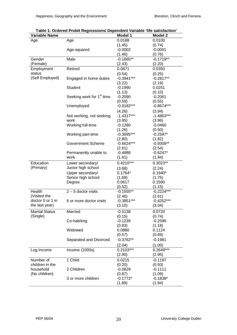
Table 1 shows the results from the estimation of our models. Following the recent literature
(e.g., Ferrer-i-Carbonell and Gowdy, 2007) and given the ordered nature of our dependent
variable, it contains results from ordered-probit regressions.15 The reference groups for the
independent variables are in parentheses.
- Table 1 about here -
The results on the socio-economic and socio-demographic characteristics in Model 1 are,
broadly speaking, in line with previous findings in the economic psychology literature. For
example, the coefficient on being unemployed is negative and significant and, everything else
being equal, reduces life satisfaction substantially (see e.g., Blanchflower and Oswald, 2004a
for similar results). Gender is significant and negative, indicating that males are less satisfied
with their lives than females. Except for the study of Alesina et al., (2004) that finds gender to
be significantly related to life satisfaction in the USA, in previous studies gender tends to
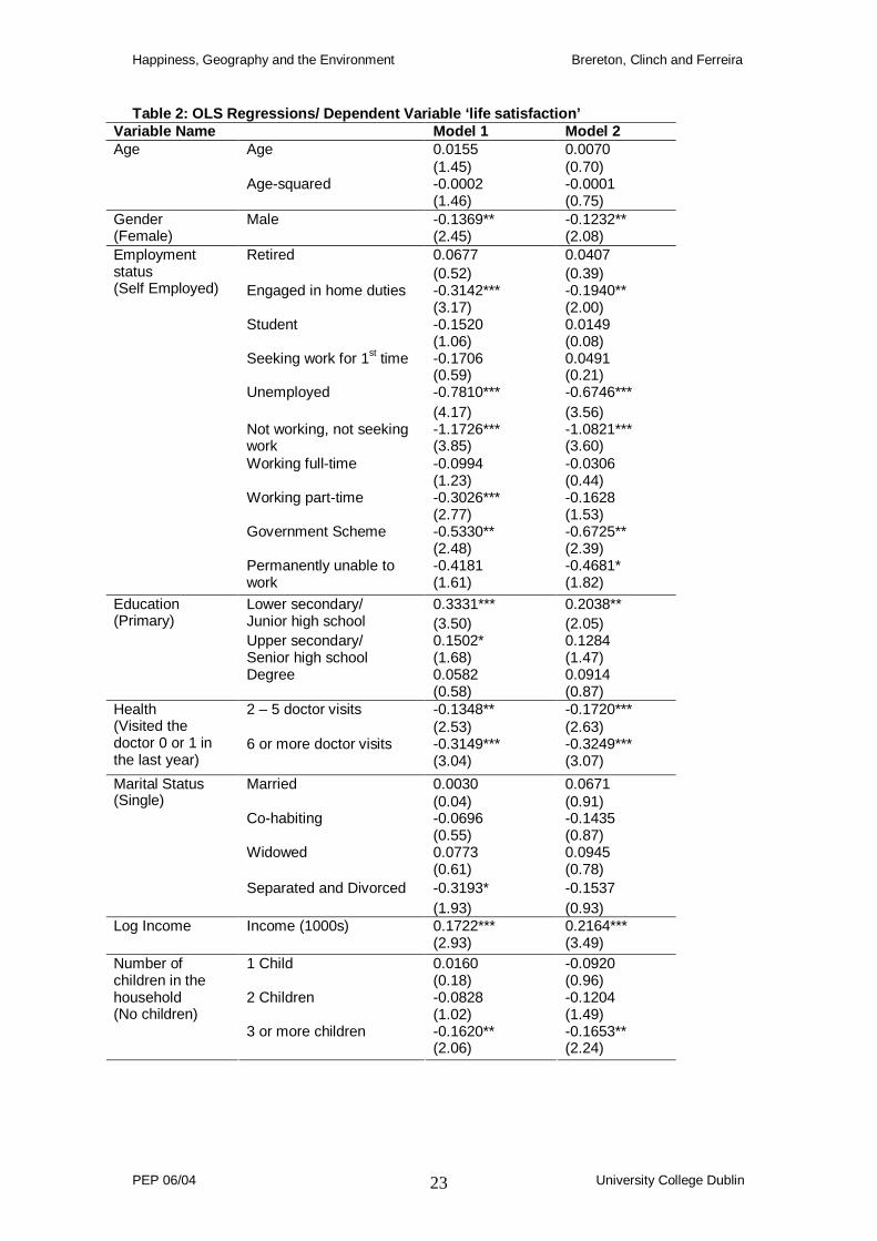
15 We also estimate OLS regressions (Table 2) and the results are comparable.
Happiness, Geography and the Environment Brereton, Clinch and Ferreira
PEP 06/04 University College Dublin 12
emerge as insignificant in life satisfaction regressions (Stutzer, 2004; Frey and Stutzer, 2000;
Di Tella et al., 2001). We find that those with lower (junior high school) or higher (senior high
school) education are more satisfied with life than those with a primary education level
(similar to Frey and Stutzer, 2000). As in Clark and Oswald (1994) and Blanchflower and
Oswald (2004b), being separated or divorced is negative and significant. However, we find no
difference between married and single respondents. Having three or more children is negative
and significant at the 5 percent level (similar to Clark and Oswald, 1994). Respondents
visiting their doctor two or more times a year are found to be less satisfied with life than those
not attending or attending only once. Living in public housing is significant and negatively
related to life satisfaction at the 1 percent level with a large coefficient. Perhaps surprisingly,
being the carer of a disabled family member emerges as positive and significant in the
regression. In line with the standard textbook prediction of utility as an increasing function of
income, our proxy for utility (life satisfaction) is an increasing function of (log) income, which
emerges significant at the 1% level. Age emerges insignificant in the regression. This is in
contrast to the international literature which, generally, finds a U-shaped association between
life satisfaction and age.
Examining the influence of location on well-being, we find the coefficient on the dummy
variable for Dublin to be highly significant and large; only the coefficients for being
unemployed and a discouraged worker are larger in magnitude (see below). Everything else
being equal, those living in all areas outside Dublin have a higher life satisfaction. This result
is similar to that in Ferrer-i-Carbonell and Gowdy (2007), who find individuals living in Inner
London to be less happy, everything else given.
Having controlled for a large number of socio-economic and socio-demographic
characteristics, a reasonable hypothesis is that factors related to the size of the settlement
and other location-specific factors may be responsible for lower life-satisfaction levels in
Dublin. For example, compared to any other area in the country, unparalleled growth rates
have resulted in the capital having a much higher population density than other areas and a
significant traffic congestion problem (DELG, 2002b). To test this hypothesis, Model 2
examines the importance of spatial amenities.
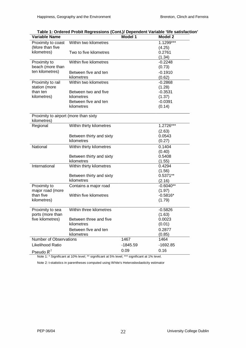
III.II. Model 2
Model 2, the results of which are reported in the fourth column of Table 1, corresponds to
Equation (1). It builds on Model 1 by including the variables with a spatial influence on well-
being. These include population density, congestion, commuting time and the climatic and
environmental variables. In this model, the dummy for Dublin loses its significance. This result
Happiness, Geography and the Environment Brereton, Clinch and Ferreira
PEP 06/04 University College Dublin 13
suggests that the spatial variables explain an important part of the difference between living in
Dublin and other regions of Ireland in terms of well-being.16
The pseudo-R 2 of Model 2, at 0.16, (adjusted-R 2 equals 0.33) exceeds all those obtained to
date in the international literature using a cross-sectional dataset. For example, Ferrer-i-
Carbonell and Gowdy (2007) in their study of subjective well-being and environmental
attitudes, obtain a pseudo-R 2 of 0.088, while Stutzer (2004), in his analysis of Swiss cantons,
obtains an R 2 of 0.11. Since we control for similar socio-economic and demographic
characteristics of the individual as in those studies, we believe this high R 2 highlights the
substantial influence of spatial amenities as determinants of well-being.17
Of the climate variables, the coefficient on mean annual precipitation is positive indicating
that, for Irish people, increased rainfall slightly increases life satisfaction. This result may,
however, be driven by a positive correlation between rain and scenic beauty.18 The most
spectacular landscapes in Ireland are found in the wettest counties in the West of Ireland.
Rehdanz and Maddison (2005) find very scarce precipitation reduces happiness, which they
hypothesize might reflect the fact that climate could have an indirect effect on happiness
through landscape effects. However, in our case the coefficient emerges insignificant at
conventional levels. Increases in the January minimum and July maximum temperatures
emerge as amenities and increase life satisfaction. Wind speed emerges negative and
significant in our regression, while surprisingly, we find that total annual sunshine is negatively
related to life satisfaction. However, it is highly likely that this result is driven by the correlation
between higher rainfall and less sunshine.
As in the hedonic literature (e.g., Blomquist et al., 1988), we find the presence of waste
facilities in an individual’s area to be a disamenity. However, the type of, and distance from,
the waste facility in question matters. The coefficient on the variable capturing if a landfill site
is in operation in the respondent’s electoral division emerges negative and significant
compared to those who live in electoral divisions more than ten kilometres away. There is
evidence suggesting that noise, smell and other negative externalities from waste facilities of
this kind may impact negatively on well-being or quality of life (DG Environment, 2000).
Proximity to a hazardous waste facility however, does not seem to have an influence in terms
of life satisfaction. It may be that individuals are less aware of the presence of these facilities
16 We also estimate Model 2 without the Dublin dummy variable and the results are almost identical (results available on request from the authors).
17 Additional R2
obtained in the literature include Blachflower and Oswald (2004b) at 0.10, Di Tella et al. (2001) at 0.17 and Blanchflower and Oswald (2004a) at 0.084. However, these papers use pooled data over a number of years and hence, may not be directly comparable. 18 A high correlation coefficient is observed between precipitation and presence of Natural Heritage Areas (0.5874), the latter being EU-designated as areas of outstanding natural beauty.
Happiness, Geography and the Environment Brereton, Clinch and Ferreira
PEP 06/04 University College Dublin 14
in their areas. The coefficient on population density is positive and significant at the 5 percent
level. This result is similar to that of Roback (1982), who finds population density to be an
amenity. Average commuting time and congestion emerge insignificant in the regression as
does the crime rate.
Proximity to coast emerges positive and significant with a large coefficient, indicating that
individuals living near the coast enjoy higher life satisfaction, other things being equal.
Additionally there is evidence that the utility value of coast is a function of distance with
respondents living two kilometres or less from the coast more satisfied with their lives,
compared to those living more than five kilometres from the coast. Those living between two
and five kilometres from the coast are also more satisfied, if insignificantly so, but the
coefficient is reduced. Interestingly, proximity to beach emerges insignificant in the
regression. It may be that, given Ireland’s climate, the amenity value of coastal areas is not a
function of the availability of a beach.
We find access to transport emerges as both an amenity and disamenity, depending on the
type of, and distance from, the amenity in question. Life satisfaction is highest for those living
between thirty and sixty kilometres from an international airport. It may be that those less than
thirty kilometres away are affected by the noise disamenity. In relation to regional airports, the
amenity value lies at less than thirty kilometres. This result is not unexpected as these are
small airports and only deal with smaller, less noisy aircraft and would have significantly fewer
arrivals and departures than do the larger airports. Close proximity to a major road (less than
five kilometres) emerges as a disamenity, again with distance decay. This may be capturing
the noise affects of this transport route. Close proximity to a seaport emerges insignificant in
the regression.
IV. Conclusion
Western governments tend to equate societal welfare with economic measures such as GDP
and GNP, prioritising macroeconomic growth in the assumption that this will bring sufficient
benefits and revenue to offset any consequent environmental or social costs. However, the
use of monetary indicators alone to measure performance runs the risk of leaving
governments in the position of having to resolve subsequent social or environmental
problems, such as inequality, past pollution or excessive carbon emissions. In this paper, we
adopt a holistic approach to the examination of the influence of geography and the
environment on happiness with an aim to informing government policy decisions. Using GIS
we are able to overcome many of the difficulties that have prevented previous researchers
addressing this issue comprehensively. This is achieved by matching individuals to their
surroundings at a higher level of disaggregration and by expanding the vector of spatial
Happiness, Geography and the Environment Brereton, Clinch and Ferreira
PEP 06/04 University College Dublin 15
variables included in the happiness function. We also use proximity measures to examine if
the influence of spatial amenities on life satisfaction is a function of distance.
The findings show that climate has a significant influence on well-being, with wind speed
negative and significant, but increases in both January minimum temperature and July
maximum temperature are positive and significant. Access to major transport routes and
proximity to coast and to waste facilities all influence well-being. However, the manner in
which they enter the happiness equation differs depending on the amenity in question.
Proximity to landfill is found to have a negative affect on well-being. Proximity to coast has a
large positive effect, but its influence is a diminishing function of distance. Additionally, the
impact of proximity to major transport routes has different effects depending on the type of,
and distance to, the amenity in question, e.g., while reasonable proximity to international
airports increases well-being, close proximity to major roads decreases it. It may be that, in
the former case, the positive effect of access outweighs the negative effect of noise, while the
opposite may be true in the latter case.
Our findings highlight the critical importance of the role of the spatial dimension in determining
well-being, i.e., spatial variables are found to be highly significant with large coefficients. In
fact, the explanatory power of our happiness function substantially increases when the spatial
variables are included, resulting in three-times the variation in well-being being explained than
has been achieved in any previous cross-sectional study. This indicates that geography and
the environment have a much larger influence on well-being than previously thought, as
important as the most critical socio-economic and socio-demographic factors, such as
unemployment and marital status. This finding has potentially important implications for
setting priorities for public policy as, in essence, improving well-being could be considered to
be the ultimate goal of public policy.
Happiness, Geography and the Environment Brereton, Clinch and Ferreira
PEP 06/04 University College Dublin 16
References Alesina, Alberto; Di Tella, Rafael and MacCulloch, Robert. “Inequality and Happiness: Are
Europeans and Americans Different?” Journal of Public Economics, 2004, 88, pp. 2009 - 2042.
Baranzini, Andrea, and Ramirez, Jose, V. “Paying for Quietness: The Impact of Noise on Geneva Rents.” Urban Studies, 2005, 42, 4, pp. 633 – 646.
Bastian, Chris, T.; McLeod, Donald, M.; Germino, Matthew, J.; Reiners, William, M. and Blasko, Benedict, J. “Environmental Amenities and Agricultural Land Values: A Hedonic Model using Geographic Information Systems data.” Ecological Economics, 2002, 40, pp. 337 – 349.
Bateman, Ian J., Jones, A.P., Lovett, I.R. and Day, B.H. “Applying Geographical Information Systems (GIS) to Environmental and Resource Economics.” Environmental and Resource Economics, 2002, 22, pp. 219 – 269.
Bateman, Ian; Day, B.; Lake, I. and Lovett, Andrew. The effect of road traffic on residential property values: a literature review and hedonic price study. Scottish Executive Transport Research Series. Edinburgh: The Stationary Office, 2001.
Berger, Mark C.; Blomquist Glenn C. and Sabirianova, Peter, Klara, “Compensating Differentials in Emerging Labour and Housing Markets: Estimates of Quality of Life in Russian Cities.” IZA Discussion Paper No. 900, October 2003.
Blanchflower, David G. and Oswald, Andrew J. “Well-being over Time in Britain and the USA.” Journal of Public Economics, 2004a, 88, pp. 1359 – 1386.
_____. “Money, Sex and Happiness: An Empirical Study.” Scandinavian Journal of Economics, 2004b, 106 (3), pp. 393 – 415.
Blomquist, Glen C.; Berger, Mark C. and Hoehn, John P. “New Estimates of Quality of Life in Urban Areas.” American Economic Review, 1988, 78 (1), pp. 89 – 107.
Bond, Derek and Devine, Paula. “The Role of Geographic Information Systems in Survey Analysis.” The Statistician, 1991, 40 (2), pp. 209 – 216.
Chay, Kenneth, Y. and Greenstone, Michael. “Does Air Quality Matter: Evidence from the Housing Market.” Journal of Political Economy, 2005, 113 (2), pp. 376 – 424.
Clark, Andrew .E. and Oswald, Andrew J. “Unhappiness and Unemployment.” Economic Journal, 1994, 104, pp. 648 – 659.
Clinch, J. Peter; Convery, Frank and Walsh, Brendan M. After the Celtic Tiger: Challenges Ahead, O’Brien Press, Dublin, 2002.
Collins, J. F. and Cummins, Thomas (eds). Agroclimatic Atlas of Ireland: Working Group on Applied Meteorology, University College Dublin, Ireland, 1996.
Craglia, Massimo; Haining, Robert and Signoretta, Paola. “Modelling High-intensity Crime Areas in English Cities.” Urban Studies, 2001, 38, 11, pp. 1921 – 1941.
CSO. Census 2002: Volume 1, Population Classified by Area. Dublin: Central Statistics Office, 2003.
_____. Quarterly National Household Survey. Dublin: Central Statistics Office, Feb 2006.
DELG. Irish Bulletin of Vehicle and Driver Statistics. Dublin: Stationary Office, Dec., 2002a.
Happiness, Geography and the Environment Brereton, Clinch and Ferreira
PEP 06/04 University College Dublin 17
_____. The National Spatial Strategy 2002-2020. Dublin: Stationary Office, Dec., 2002b.
Diener, Ed and Suh, Mark Eunkook. “National Differences in Subjective Well-being”, in Kahneman, D., Diener, E, Schwarz, N. (eds.), Well-being: The Foundations of Hedonic Psychology. Russell Sage Foundation, New York, 1999.
Diener, Ed., Suh, E. M., Lucas, Richard E. and Smith, H.L. “Subjective Well-being: Three Decades of Progress.” Psychological Bulletin, 1999, 125, pp. 276 – 302.
Din, Allan; Hoesli, Martin and Bender, Andre. “Environmental Variables and Real Estate Prices.” Urban Studies, 2001, 28, 11, pp. 1989 – 2000.
Di Tella, Raphael; MacCulloch, Robert J. and Oswald Andrew J. “Preferences over Inflation and Unemployment: Evidence from Surveys of Happiness.” American Economic Review, 2001, 91, pp. 335 – 341.
DG Environment, A Study on the Economic Valuation of Environmental Externalities from Landfill Disposal and Incineration of Waste, Final Main Report, European Commission, Brussels October 2000.
Easterlin, Richard A. “Does Economic Growth Improve the Human Lot?” in Paul A. David and Melvin W. Reder, (eds.), Nations and Households in Economic Growth: Essays in Honor of Moses Abramovitz, Academic Press, New York, 1974.
_____. “Will Raising the Incomes of All Increase the Happiness of All?” Journal of Economic Behaviour and Organisation, 1995, 27, pp. 35 – 47.
_____. “Income and Happiness: Towards a Unified Theory.” Economic Journal, 2001, 111, pp. 465 – 484.
Economist Intelligence Unit’s Quality of Life Index. London: The Economist, 2004.
EPA. Ireland’s Environment. Wexford: Environmental Protection Agency, 2004.
_____. National Waste Database. Wexford: Environmental Protection Agency, 2005.
Ferrer-i-Carbonell, Ada and Frijters, Paul. “How Important Is Methodology for the Estimates of the Determinants of Happiness?” Economic Journal, 2004, 114 (497) pp. 641 - 659.
Ferrer-i-Carbonell, Ada and Gowdy, John, M. “Environmental Degradation and Happiness?” Ecological Economics, 2007, 60 (3) pp. 509 - 516.
Frey, Bruno S. and Stutzer, Alois. “Happiness, Economy and Institutions.” Economic Journal, 2000, 110, pp. 918 – 938.
_____. Happiness and Economics. Princeton University Press, Princeton, 2002a.
_____. “What can Economists Learn from Happiness Research?” Journal of Economic Literature, 2002b, 40 (2), pp. 402 – 435.
_____. “Stress that Doesn’t Pay: The Commuting Paradox.” IZA Discussion Paper No 1278, 2004.
Frijters, Paul and Van Praag, Bernard, M. S. “The Effects of Climate on Welfare and Well-being in Russia?” Climate Change, 1998, 39, pp. 61 - 81.
Garda Siochana. Annual Report. Dublin: Garda Siochana, 2002.
Happiness, Geography and the Environment Brereton, Clinch and Ferreira
PEP 06/04 University College Dublin 18
Geoghegan, J., Wainger, L.A. and Bockstaell, N.E. “Spatial Landscape Indices in a Hedonic Framework: an Ecological Economics Analysis using GIS.” Ecological Economics, 1997, 23, pp. 251 – 264.
Goodchild, Michael, F. and Haining, Robert, P. “GIS and Spatial Data Analysis: Converging Perspectives.” Papers in Regional Science, 2004, 83, pp. 363 – 385.
Kavanagh, Adrian, Mills, Gerald and Sinnot, Richard. “The Geography of Irish Voter Turnout: A Case Study of the 2002 General Election.” Irish Geography, 2004, 37 (2), pp. 177 – 186.
Lake, I.R., Lovett, A.A, Bateman, I.J. and Langford, I.H. “Modeling Environmental Influences on Property Prices in an Urban Environment.” Computer, Environment and Urban Systems, 1998, 22 (2), pp. 121 – 136.
Luttmer, Erzo, F. P. “Neighbors as Negatives: Relative Earnings and Well-Being.” Quarterly Journal of Economics, 2004, CXX (3), pp. 963 – 1002.
Lynch, Allen, K. and Rasmussen, David, W. “Proximity, Neighbour and the Efficiency of Exclusion.” Urban Studies, 2001, 41, 2, pp. 285 – 298.
Moulton, Brent R. “An Illustration of a Pitfall in Estimating the Effects of Aggregate Variables on Micro Units”. Review of Economics and Statistics, 1990, 72 (2), pp 334 – 338.
NRA. National Route Lengths. Dublin: National Road Authority, 2003.
Oswald, Andrew J. “Happiness and Economic Performance”, Economic Journal, 1997, 107 (445), pp. 1815 – 1831.
Paterson, Robert, P. and Boyle, Kevin, J. “Out of Sight, Out of Mind? Using GIS to Incorporate Visibility in Hedonic Property Value Models.” Land Economics, 2002, 78, 3, pp. 417 – 425.
Peiro, Amado. “Happiness, Satisfaction and Socio-economic Conditions: Some International Evidence.” Journal of Socio-Economics, 2006, 35, pp. 348 – 365.
Putnam, Robert D. Bowling Alone: The Collapse and Revival of American Community, Touchstone, New York, 2000.
Rehdanz, Katrin and Maddison, David. “Climate and Happiness.” Ecological Economics, 2005, 52, pp. 111- 125.
Roback, Jennifer. “Wages, Rents and the Quality of Life.” Journal of Political Economy, 1982, 90 (6), pp. 1257 – 1278.
Rosen, Sherwin. “Hedonic Prices and Implicit Markets: Product Differentiation in Pure Competition.” Journal of Political Economy, 1974, 82, pp. 34 – 55.
Stutzer, Alois. “The Role of Income Aspirations in Individual Happiness.” Journal of Economic Behaviour and Organization, 2004, 54 (1), pp. 89 - 109.
UII. Urbis Database. Dublin: Urban Institute Ireland, 2006.
Van Praag, Bernard, M. S. and Baarsma, Barbara, E. “Using Happiness Surveys to Value Intangibles: The Case of Airport Noise.” Economic Journal, 2005, 115, pp 224 – 246.
Veenhoven, Ruut. “Advances in the Understanding of Happiness.” Revue Québécoise de Psychologie, 1997, 18 (2), pp. 29 – 74.

Happiness, Geography and the Environment Brereton, Clinch and Ferreira
PEP 06/04 University College Dublin 19
Welsch, Heinz. "Environment and Happiness: Valuation of Air Pollution Using Life Satisfaction Data." Ecological Economics, 2006, 58, pp. 801 - 813.
Wu, Yi-Hwa; Miller, Havery, J. and Hung, Ming-Chih. “A GIS-based Decision Support System for Analysis of Route Choice in Congested Urban Road Networks.” Journal of Geographical Systems, 2001, 3, pp. 3 – 24.
Happiness, Geography and the Environment Brereton, Clinch and Ferreira
PEP 06/04 University College Dublin 20
Table 1: Ordered Probit Regressions/ Dependent Vari able ‘life satisfaction’ Variable Name Model 1 Model 2
Age 0.0188 0.0100 (1.45) (0.74) Age-squared -0.0002 -0.0001
Age
(1.46) (0.76) -0.1665** -0.1719** Gender
(Female) Male
(2.43) (2.20) 0.0871 0.0350 Retired (0.54) (0.25) -0.3941*** -0.2817** Engaged in home duties (3.22) (2.19) -0.1990 0.0251 Student
(1.13) (0.10) -0.2090 -0.2061 Seeking work for 1st time (0.59) (0.55) -0.9182*** -0.8674*** Unemployed
(4.26) (3.94) -1.4317*** -1.4863*** Not working, not seeking
work (3.95) (3.96) -0.1280 -0.0460 Working full-time (1.26) (0.50) -0.3695*** -0.2597* Working part-time (2.80) (1.82) -0.6624*** -0.9309** Government Scheme (2.61) (2.54) -0.4888 -0.6247*
Employment status (Self Employed)
Permanently unable to work (1.61) (1.94)
0.4210*** 0.3023** Lower secondary/ Junior high school (3.68) (2.24)
0.1764* 0.1940* Upper secondary/ Senior high school (1.69) (1.75)
0.0617 0.1590
Education (Primary)
Degree (0.52) (1.15)
-0.1555** -0.2224*** 2 – 5 doctor visits (2.46) (2.61) -0.3851*** -0.4252***
Health (Visited the doctor 0 or 1 in the last year)
6 or more doctor visits (3.10) (3.04)
-0.0138 0.0720 Married (0.15) (0.74) -0.1239 -0.2596 Co-habiting (0.83) (1.18) 0.0880 0.1124 Widowed (0.57) (0.69) -0.3762** -0.1981
Marital Status (Single)
Separated and Divorced (2.04) (1.00) 0.2103*** 0.2649*** Log Income Income (1000s) (2.90) (2.95) 0.0215 -0.1197 1 Child (0.20) (0.93) -0.0829 -0.1111 2 Children (0.87) (1.09) -0.1772* -0.1838*
Number of children in the household (No children)
3 or more children (1.89) (1.94)

Happiness, Geography and the Environment Brereton, Clinch and Ferreira
PEP 06/04 University College Dublin 21
Table 1: Ordered Probit Regressions (cont.)/ Depend ent Variable ‘life satisfaction’ Variable Name Model 1 Model 2
Own with a mortgage -0.0194 0.0156 (0.27) (0.20) Rent privately 0.0342 -0.0033 (0.27) (0.02) Public housing -0.5125*** -0.4781***
Household tenure (Own Outright)
(4.69) (3.61) Respondent is a carer 0.3314* 0.2313 (1.70) (1.24) Dublin Dummy Variable -0.7527*** -0.4430 (11.79) (1.12) Spatial Variables No Yes
0.0005 Precipitation (1.28) -0.3815** Wind speed (2.36) 0.8082*** January minimum
temperature (3.33) 0.0806*** July maximum
temperature (3.85) -0.0011
Climate Variables
Average annual sunshine (hours) (1.22)
0.0057 Average commuting time (0.48) 0.0061* Population density
(1.92) -0.0001 Congestion
(1.17) 0.0570 Homicide rate
(0.97) 0.0160* Voter turnout
(1.84)
-0.5145* Contains a landfill (1.87) 0.4332 Within three kilometres (1.55) 0.2998 Between three and five
kilometres (0.95) -0.2359
Proximity to landfill (More than ten kilometres)
Between five and ten kilometres (1.40)
-0.4190 Contains a hazardous waste facility (0.71)
-0.1993 Within three kilometres (0.54) -0.3983 Between three and five
kilometres (1.01) -0.2888
Proximity to hazardous waste facility (More than ten kilometres)
Between five and ten kilometres (0.89)
Happiness, Geography and the Environment Brereton, Clinch and Ferreira
PEP 06/04 University College Dublin 22
Table 1: Ordered Probit Regressions (Cont.)/ Dependent Variable ‘life satisfaction’ Variable Name Model 1 Model 2
1.1299*** Within two kilometres (4.25) 0.2761
Proximity to coast (More than five kilometres) Two to five kilometres
(1.34) -0.2248 Within five kilometres (0.73) -0.1910
Proximity to beach (more than ten kilometres) Between five and ten
kilometres (0.62) -0.2868 Within two kilometres (1.28) -0.3531 Between two and five
kilometres (1.37) -0.0391
Proximity to rail station (more than ten kilometres)
Between five and ten kilometres (0.14)
Proximity to airport (more than sixty kilometres)
1.2726*** Within thirty kilometres (2.63) 0.0543
Regional
Between thirty and sixty kilometres (0.27)
0.1404 Within thirty kilometres (0.40) 0.5408
National
Between thirty and sixty kilometres (1.55)
0.4294 Within thirty kilometres (1.56) 0.5371**
International
Between thirty and sixty kilometres (2.16)
-0.6040** Contains a major road (1.97) -0.5816*
Proximity to major road (more than five kilometres)
Within five kilometres (1.79)
-0.5826 Within three kilometres (1.63) 0.0023 Between three and five
kilometres (0.01) 0.2877
Proximity to sea ports (more than five kilometres) Between five and ten
kilometres (0.85) Number of Observations 1467 1464 Likelihood Ratio -1845.59 -1692.85
Pseudo 2R 0.09 0.16 Note 1: * Significant at 10% level; ** significant at 5% level; *** significant at 1% level.
Note 2: t-statistics in parentheses computed using White’s Heteroskedasticity estimator
Happiness, Geography and the Environment Brereton, Clinch and Ferreira
PEP 06/04 University College Dublin 23
Table 2: OLS Regressions/ Dependent Variable ‘life satisfaction’ Variable Name Model 1 Model 2
Age 0.0155 0.0070 (1.45) (0.70) Age-squared -0.0002 -0.0001
Age
(1.46) (0.75) -0.1369** -0.1232** Gender
(Female) Male
(2.45) (2.08) 0.0677 0.0407 Retired (0.52) (0.39) -0.3142*** -0.1940** Engaged in home duties (3.17) (2.00) -0.1520 0.0149 Student
(1.06) (0.08) -0.1706 0.0491 Seeking work for 1st time (0.59) (0.21) -0.7810*** -0.6746*** Unemployed
(4.17) (3.56) -1.1726*** -1.0821*** Not working, not seeking
work (3.85) (3.60) -0.0994 -0.0306 Working full-time (1.23) (0.44) -0.3026*** -0.1628 Working part-time (2.77) (1.53) -0.5330** -0.6725** Government Scheme (2.48) (2.39) -0.4181 -0.4681*
Employment status (Self Employed)
Permanently unable to work (1.61) (1.82)
0.3331*** 0.2038** Lower secondary/ Junior high school (3.50) (2.05)
0.1502* 0.1284 Upper secondary/ Senior high school (1.68) (1.47)
0.0582 0.0914
Education (Primary)
Degree (0.58) (0.87)
-0.1348** -0.1720*** 2 – 5 doctor visits (2.53) (2.63) -0.3149*** -0.3249***
Health (Visited the doctor 0 or 1 in the last year)
6 or more doctor visits (3.04) (3.07)
0.0030 0.0671 Married (0.04) (0.91) -0.0696 -0.1435 Co-habiting (0.55) (0.87) 0.0773 0.0945 Widowed (0.61) (0.78) -0.3193* -0.1537
Marital Status (Single)
Separated and Divorced (1.93) (0.93) 0.1722*** 0.2164*** Log Income Income (1000s) (2.93) (3.49) 0.0160 -0.0920 1 Child (0.18) (0.96) -0.0828 -0.1204 2 Children (1.02) (1.49) -0.1620** -0.1653**
Number of children in the household (No children)
3 or more children (2.06) (2.24)
Happiness, Geography and the Environment Brereton, Clinch and Ferreira
PEP 06/04 University College Dublin 24
Table 2: OLS Regressions (Continued)/ Dependent Variable ‘life satisfaction’ Variable Name Model 1 Model 2
Own with a mortgage -0.0061 0.0149 (0.10) (0.25) Rent privately 0.0309 0.0100 (0.30) (0.08) Public housing -0.4379*** -0.3594***
Household tenure (Own Outright)
(4.81) (3.52) Respondent is a carer 0.2632* 0.2371* (1.73) (1.91) Dublin dummy variable -0.6222*** -0.2434 (11.43) (0.78) Spatial Variables No Yes
-0.0003 Precipitation (1.05) -0.2459** Wind speed (2.13) 0.5558*** January minimum
temperature (3.19) 0.0543*** July maximum
temperature (3.77) -0.0011*
Climate Variables
Average annual sunshine (hours) (1.74)
0.0034 Average commuting time (0.41) 0.0038 Population density
(1.63) -0.0001 Congestion
(1.36) 0.0501 Homicide rate
(1.06) 0.0124** Voter turnout
(2.12) -0.3736* Contains a landfill (1.90) 0.2646 Within three kilometres (1.32) 0.2564 Between three and five
kilometres (1.05) -0.1346
Proximity to landfill (More than ten kilometres)
Between five and ten kilometres (1.07)
-0.2068 Contains a hazardous waste facility (0.47)
-0.1715 Within three kilometres (0.64) -0.2998 Between three and five
kilometres (1.03) -0.1560
Proximity to hazardous waste facility (More than ten kilometres)
Between five and ten kilometres (0.66)
Happiness, Geography and the Environment Brereton, Clinch and Ferreira
PEP 06/04 University College Dublin 25
Table 2: OLS Regressions (Continued)/ Dependent Variable ‘life satisfaction’ Variable Name Model 1 Model 2
0.8351*** Within two kilometres (4.32) 0.2271
Proximity to coast (More than five kilometres) Two to five kilometres
(1.51) -0.1607 Within five kilometres (0.73) -0.0923
Proximity to beach (more than ten kilometres) Between five and ten
kilometres (0.42) -0.1705 Within two kilometres (1.07) -0.2271 Between two and five
kilometres (1.22) -0.0142
Proximity to rail station (more than ten kilometres)
Between five and ten kilometres (0.07)
Proximity to airport (more than sixty kilometres)
0.8329*** Within thirty kilometres (2.78) 0.0284
Regional
Between thirty and sixty kilometres (0.21)
0.0721 Within thirty kilometres (0.28) 0.3383
National
Between thirty and sixty kilometres (1.44)
0.2603 Within thirty kilometres (1.30) 0.3851**
International
Between thirty and sixty kilometres (2.18)
-0.3703* Contains a major road (1.83) -0.3543
Proximity to major road (more than five kilometres)
Within five kilometres (1.62) -0.3887 Within three kilometres (1.42) 0.0019 Between three and five
kilometres (0.01) 0.2054
Proximity to sea ports (more than five kilometres) Between five and ten
kilometres (0.75) Number of Observations 1467 1451
Adjusted 2R 0.21 0.33 Note 1: * Significant at 10% level; ** significant at 5% level; *** significant at 1% level.
Note 2: t-statistics in parentheses computed using White’s Heteroskedasticity estimator
Happiness, Geography and the Environment Brereton, Clinch and Ferreira
PEP 06/04 University College Dublin 26
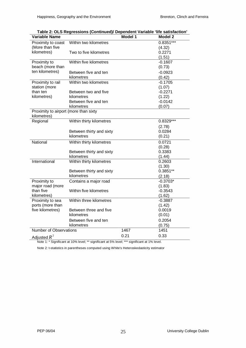
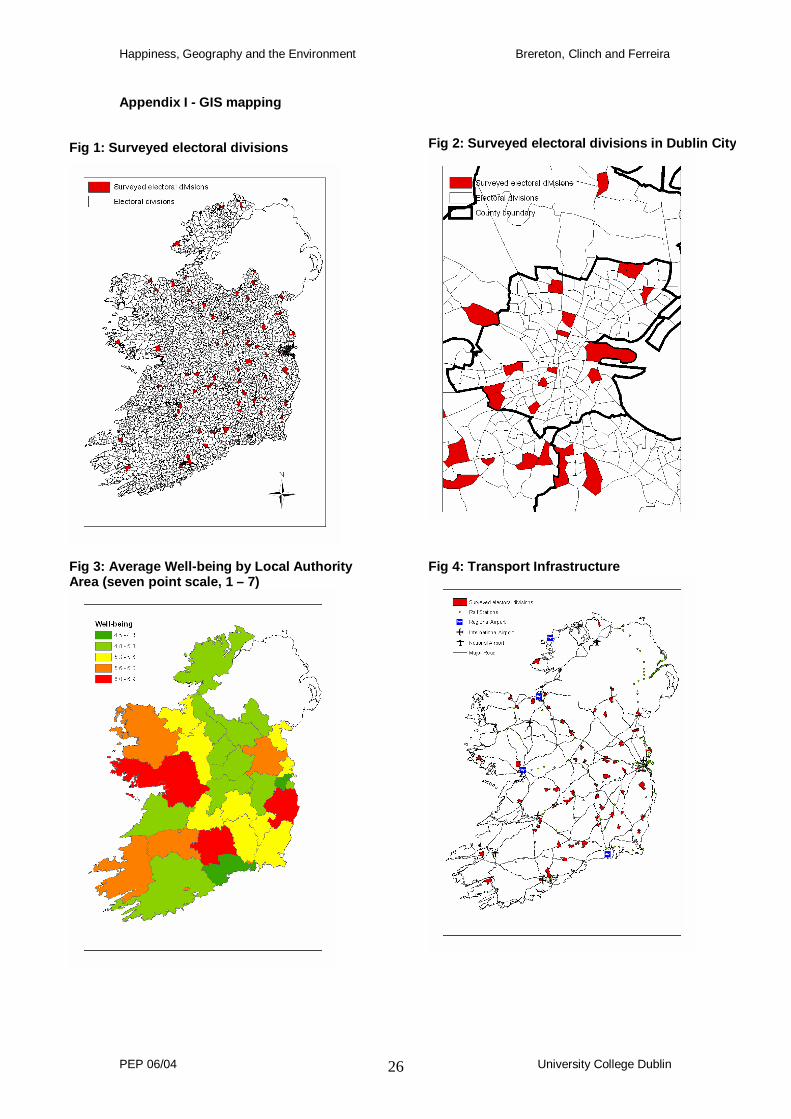
Appendix I - GIS mapping
Fig 2: Surveyed electoral divisions in Dublin City
Fig 1: Surveyed electoral divisions
Fig 3: Average Well -being by Local Authority Area (seven point scale, 1 – 7)
Fig 4: Transport Infrastructure
Happiness, Geography and the Environment Brereton, Clinch and Ferreira
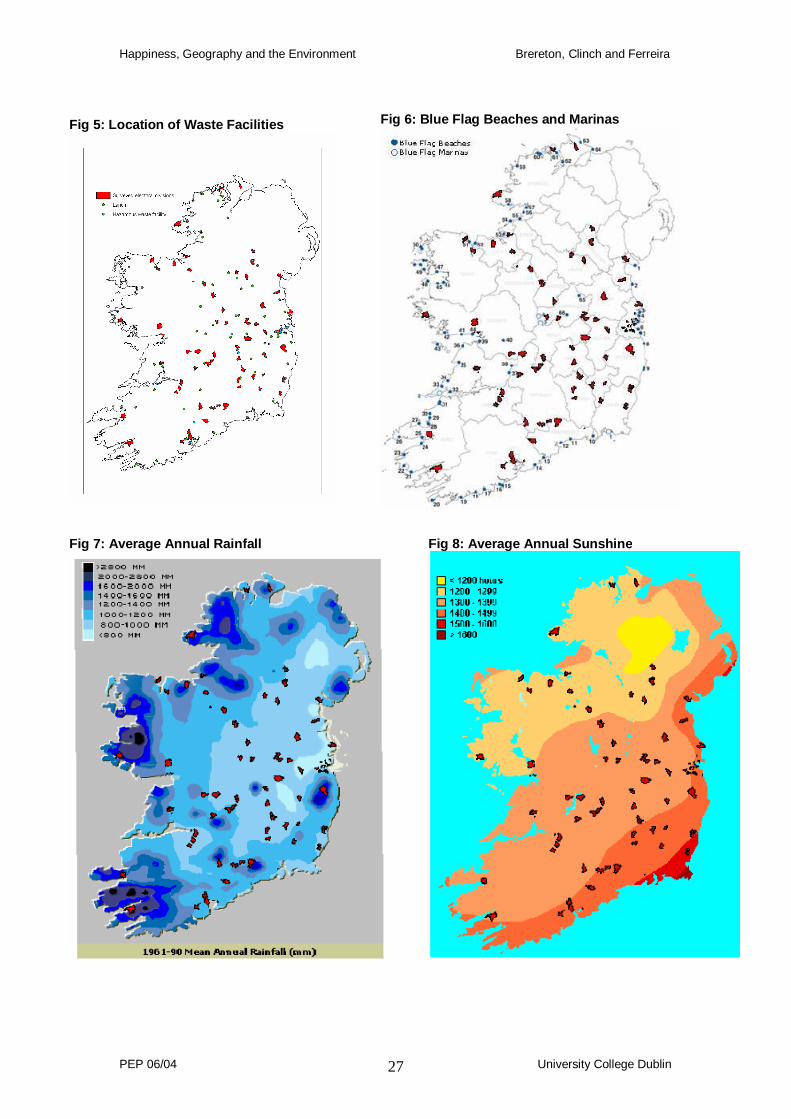
PEP 06/04 University College Dublin 27
Fig 5: Location of Waste Facilities
Fig 7: Average Annual Rainfall
Fig 8: Average Annual Sunshine
Fig 6: Blue Flag Beaches and Marinas
Happiness, Geography and the Environment Brereton, Clinch and Ferreira
PEP 06/04 University College Dublin 28
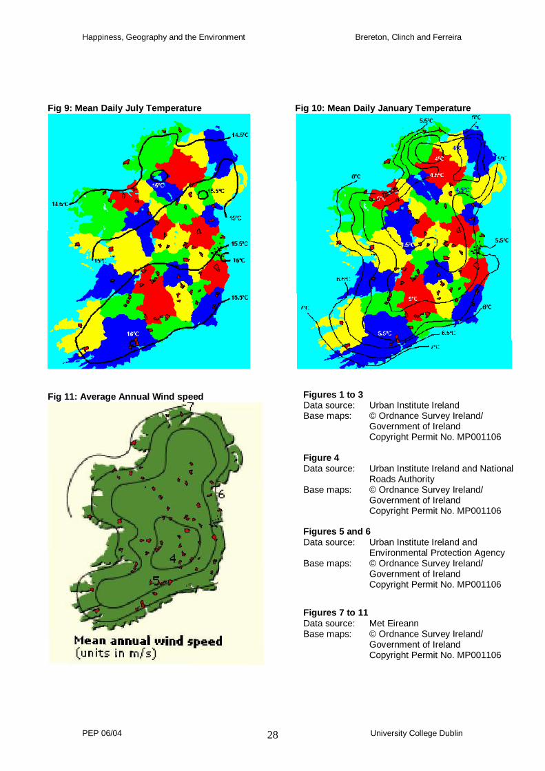
Fig 10: Mean Daily January Temperature
Fig 9: Mean Daily July Temperature
Fig 11: Average Annual Wind speed
Figures 1 to 3 Data source: Urban Institute Ireland Base maps: © Ordnance Survey Ireland/
Government of Ireland Copyright Permit No. MP001106
Figure 4 Data source: Urban Institute Ireland and National
Roads Authority Base maps: © Ordnance Survey Ireland/
Government of Ireland Copyright Permit No. MP001106
Figures 5 and 6 Data source: Urban Institute Ireland and
Environmental Protection Agency Base maps: © Ordnance Survey Ireland/
Government of Ireland Copyright Permit No. MP001106
Figures 7 to 11 Data source: Met Eireann Base maps: © Ordnance Survey Ireland/
Government of Ireland Copyright Permit No. MP001106
Happiness, Geography and the Environment Brereton, Clinch and Ferreira
PEP 06/04 University College Dublin 29
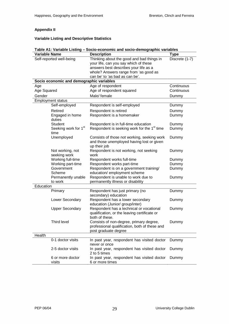
Appendix II Variable Listing and Descriptive Statistics
Table A1: Variable Listing – Socio-economic and soc io-demographic variables Variable Name Description Type Self-reported well-being
Thinking about the good and bad things in your life, can you say which of these answers best describes your life as a whole? Answers range from ‘as good as can be’ to ’as bad as can be’.
Discrete (1-7)
Socio economic and demographic variables Age Age of respondent Continuous Age Squared Age of respondent squared Continuous Gender Male/ female Dummy Employment status
Self-employed Respondent is self-employed Dummy
Retired Respondent is retired Dummy Engaged in home
duties Respondent is a homemaker Dummy
Student Respondent is in full-time education Dummy Seeking work for 1st
time Respondent is seeking work for the 1st time Dummy
Unemployed
Consists of those not working, seeking work and those unemployed having lost or given up their job
Dummy
Not working, not seeking work
Respondent is not working, not seeking work
Dummy
Working full-time Respondent works full-time Dummy Working part-time Respondent works part-time Dummy Government Scheme
Respondent is on a government training/ education/ employment scheme
Dummy
Permanently unable to work
Respondent is unable to work due to permanently illness or disability
Dummy
Education Primary Respondent has just primary (no
secondary) education Dummy
Lower Secondary Respondent has a lower secondary education (Junior/ group/inter)
Dummy
Upper Secondary Respondent has a technical or vocational qualification, or the leaving certificate or both of these.
Dummy
Third level Consists of non-degree, primary degree, professional qualification, both of these and post graduate degree
Dummy
Health 0-1 doctor visits In past year, respondent has visited doctor
never or once Dummy
2-5 doctor visits In past year, respondent has visited doctor 2 to 5 times
Dummy
6 or more doctor visits
In past year, respondent has visited doctor 6 or more times
Dummy
Happiness, Geography and the Environment Brereton, Clinch and Ferreira
PEP 06/04 University College Dublin 30
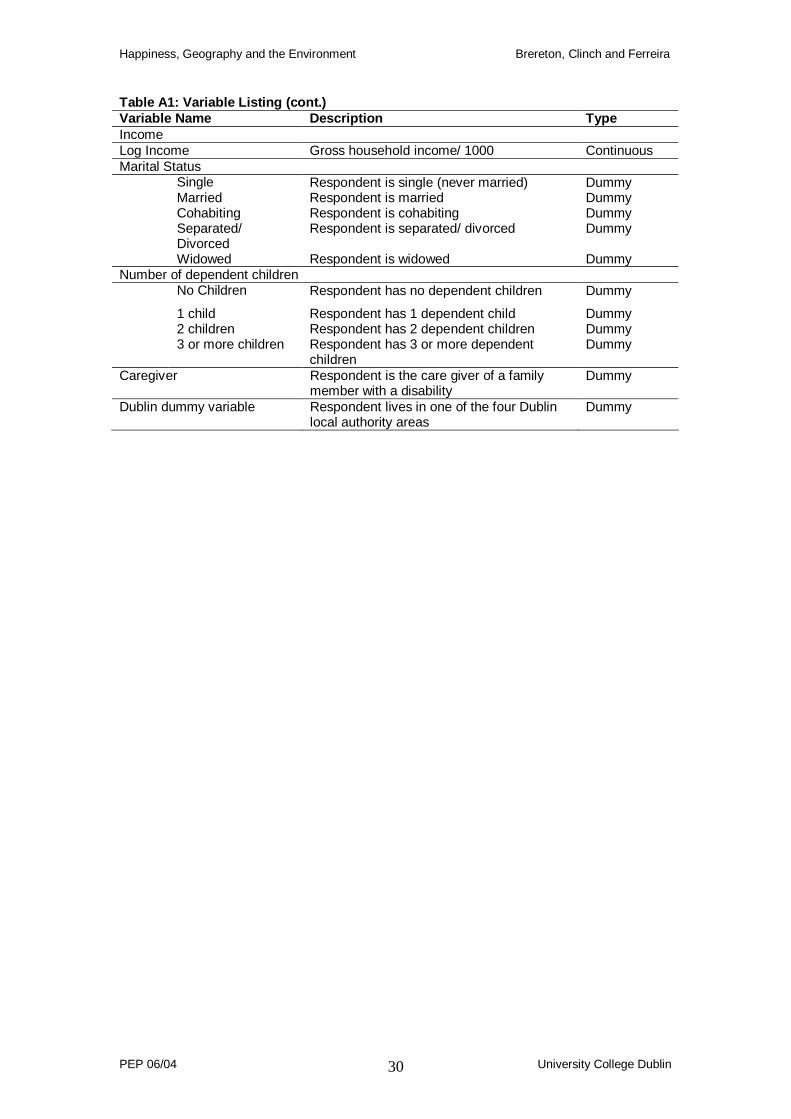
Table A1: Variable Listing (cont.) Variable Name Description Type Income Log Income Gross household income/ 1000 Continuous Marital Status
Single Respondent is single (never married) Dummy Married Respondent is married Dummy Cohabiting Respondent is cohabiting Dummy Separated/ Divorced
Respondent is separated/ divorced Dummy
Widowed Respondent is widowed Dummy Number of dependent children
No Children Respondent has no dependent children Dummy
1 child Respondent has 1 dependent child Dummy 2 children Respondent has 2 dependent children Dummy 3 or more children Respondent has 3 or more dependent
children Dummy
Caregiver Respondent is the care giver of a family member with a disability
Dummy
Dublin dummy variable
Respondent lives in one of the four Dublin local authority areas
Dummy
Happiness, Geography and the Environment Brereton, Clinch and Ferreira
PEP 06/04 University College Dublin 31
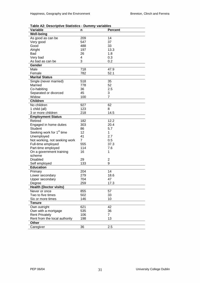
Table A2: Descriptive Statistics - Dummy variables Variable n Percent Well-being As good as can be 209 14 Very good 547 37 Good 488 33 Alright 197 13.3 Bad 26 1.8 Very bad 4 0.3 As bad as can be 3 0.2 Gender Male 718 47.9 Female 782 52.1 Marital Status Single (never married) 518 35 Married 778 52 Co-habiting 36 2.5 Separated or divorced 45 3 Widow 100 7 Children No children 927 62 1 child (all) 123 8 3 or more children 218 14.5 Employment Status Retired 182 12.2 Engaged in home duties 303 20.4 Student 86 5.7 Seeking work for 1st time 12 1 Unemployed 41 2.7 Not working, not seeking work 7 0.5 Full-time employed 555 37.3 Part-time employed 114 7.6 On a government training scheme
16 1
Disabled 29 2 Self employed 133 9 Education Primary 204 14 Lower secondary 279 18.6 Upper secondary 704 47 Degree 259 17.3 Health (Doctor visits) Never or once 855 57 Two to five times 502 33 Six or more times 146 10 Tenure Own outright 621 42 Own with a mortgage 535 36 Rent Privately 106 7 Rent from the local authority 198 13 Other Caregiver 36 2.5
Happiness, Geography and the Environment Brereton, Clinch and Ferreira
PEP 06/04 University College Dublin 32
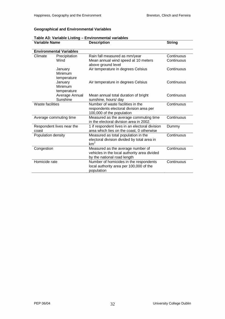
Geographical and Environmental Variables
Table A3: Variable Listing – Environmental variables Variable Name Description String
Environmental Variables Climate Precipitation Rain fall measured as mm/year Continuous Wind Mean annual wind speed at 10 meters
above ground level Continuous
January Minimum temperature
Air temperature in degrees Celsius Continuous
January Minimum temperature
Air temperature in degrees Celsius Continuous
Average Annual Sunshine
Mean annual total duration of bright sunshine, hours/ day
Continuous
Waste facilities
Number of waste facilities in the respondents electoral division area per 100,000 of the population
Continuous
Average commuting time Measured as the average commuting time in the electoral division area in 2002.
Continuous
Respondent lives near the coast
1 if respondent lives in an electoral division area which lies on the coast, 0 otherwise
Dummy
Population density Measured as total population in the electoral division divided by total area in km2
Continuous
Congestion
Measured as the average number of vehicles in the local authority area divided by the national road length
Continuous
Homicide rate
Number of homicides in the respondents local authority area per 100,000 of the population
Continuous
Happiness, Geography and the Environment Brereton, Clinch and Ferreira
PEP 06/04 University College Dublin 33
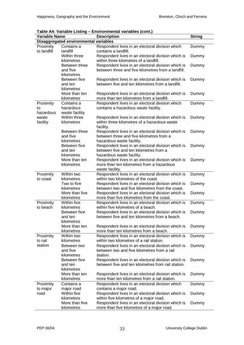
Table A4: Variable Listing – Environmental variables (cont.) Variable Name Description String Disaggregated environmental variables
Contains a landfill
Respondent lives in an electoral division which contains a landfill.
Dummy
Within three kilometres
Respondent lives in an electoral division which is within three kilometres of a landfill.
Dummy
Between three and five kilometres
Respondent lives in an electoral division which is between three and five kilometres from a landfill.
Dummy
Between five and ten kilometres
Respondent lives in an electoral division which is between five and ten kilometres from a landfill.
Dummy
Proximity to landfill
More than ten kilometres
Respondent lives in an electoral division which is more than ten kilometres from a landfill.
Dummy
Contains a hazardous waste facility
Respondent lives in an electoral division which contains a hazardous waste facility.
Dummy
Within three kilometres
Respondent lives in an electoral division which is within three kilometres of a hazardous waste facility.
Dummy
Between three and five kilometres
Respondent lives in an electoral division which is between three and five kilometres from a hazardous waste facility.
Dummy
Between five and ten kilometres
Respondent lives in an electoral division which is between five and ten kilometres from a hazardous waste facility.
Dummy
Proximity to hazardous waste facility
More than ten kilometres
Respondent lives in an electoral division which is more than ten kilometres from a hazardous waste facility.
Dummy
Within two kilometres
Respondent lives in an electoral division which is within two kilometres of the coast.
Dummy
Two to five kilometres
Respondent lives in an electoral division which is between two and five kilometres from the coast.
Dummy
Proximity to coast
More than five kilometres
Respondent lives in an electoral division which is more than five kilometres from the coast.
Dummy
Within five kilometres
Respondent lives in an electoral division which is within five kilometres of a beach.
Dummy
Between five and ten kilometres
Respondent lives in an electoral division which is between five and ten kilometres from a beach.
Dummy
Proximity to beach
More than ten kilometres
Respondent lives in an electoral division which is more than ten kilometres from a beach.
Dummy
Within two kilometres
Respondent lives in an electoral division which is within two kilometres of a rail station.
Dummy
Between two and five kilometres
Respondent lives in an electoral division which is between two and five kilometres from a rail station.
Dummy
Between five and ten kilometres
Respondent lives in an electoral division which is between five and ten kilometres from rail station.
Dummy
Proximity to rail station
More than ten kilometres
Respondent lives in an electoral division which is more than ten kilometres from a rail station.
Dummy
Contains a major road
Respondent lives in an electoral division which contains a major road.
Dummy
Within five kilometres
Respondent lives in an electoral division which is within five kilometres of a major road.
Dummy
Proximity to major road
More than five kilometres
Respondent lives in an electoral division which is more than five kilometres of a major road.
Dummy
Happiness, Geography and the Environment Brereton, Clinch and Ferreira
PEP 06/04 University College Dublin 34
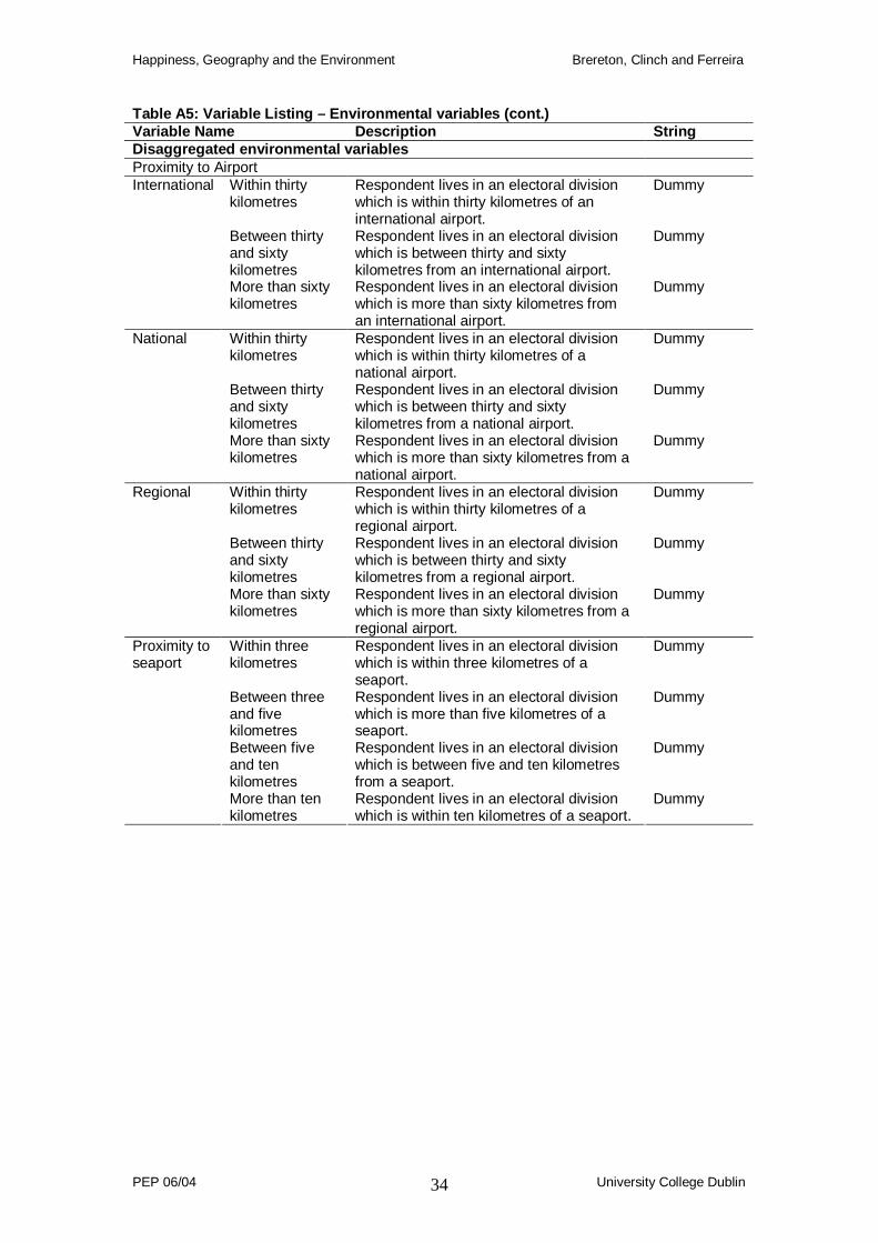
Table A5: Variable Listing – Environmental variables (cont.) Variable Name Description String Disaggregated environmental variables Proximity to Airport
Within thirty kilometres
Respondent lives in an electoral division which is within thirty kilometres of an international airport.
Dummy
Between thirty and sixty kilometres
Respondent lives in an electoral division which is between thirty and sixty kilometres from an international airport.
Dummy
International
More than sixty kilometres
Respondent lives in an electoral division which is more than sixty kilometres from an international airport.
Dummy
Within thirty kilometres
Respondent lives in an electoral division which is within thirty kilometres of a national airport.
Dummy
Between thirty and sixty kilometres
Respondent lives in an electoral division which is between thirty and sixty kilometres from a national airport.
Dummy
National
More than sixty kilometres
Respondent lives in an electoral division which is more than sixty kilometres from a national airport.
Dummy
Within thirty kilometres
Respondent lives in an electoral division which is within thirty kilometres of a regional airport.
Dummy
Between thirty and sixty kilometres
Respondent lives in an electoral division which is between thirty and sixty kilometres from a regional airport.
Dummy
Regional
More than sixty kilometres
Respondent lives in an electoral division which is more than sixty kilometres from a regional airport.
Dummy
Within three kilometres
Respondent lives in an electoral division which is within three kilometres of a seaport.
Dummy
Between three and five kilometres
Respondent lives in an electoral division which is more than five kilometres of a seaport.
Dummy
Between five and ten kilometres
Respondent lives in an electoral division which is between five and ten kilometres from a seaport.
Dummy
Proximity to seaport
More than ten kilometres
Respondent lives in an electoral division which is within ten kilometres of a seaport.
Dummy
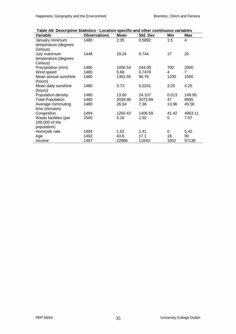
Happiness, Geography and the Environment Brereton, Clinch and Ferreira
PEP 06/04 University College Dublin 35
Table A6: Descriptive Statistics - Location-specif ic and other continuous variables Variable Observations Mean Std. Dev Min Max January minimum temperature (degrees Celsius)
1480 2.35 0.5892 1.5 4
July maximum temperature (degrees Celsius)
1448 19.24 0.744 17 20
Precipitation (mm) 1480 1000.54 244.09 700 2000 Wind speed 1480 5.68 0.7479 4 7 Mean annual sunshine (hours)
1480 1391.55 90.76 1200 1500
Mean daily sunshine (hours)
1480 3.73 0.2241 3.25 4.25
Population density 1480 13.60 24.107 0.013 149.95 Total Population 1480 2039.95 2073.69 47 8595 Average commuting time (minutes)
1480 26.54 7.36 13.96 45.56
Congestion 1494 1260.42 1406.59 41.42 4963.11 Waste facilities (per 100,000 of the population)
1500 3.19 1.92 0 7.07
Homicide rate 1494 1.52 1.41 0 5.42 Age 1492 43.6 17.1 18 90 Income 1497 22986 11643 1852 57138
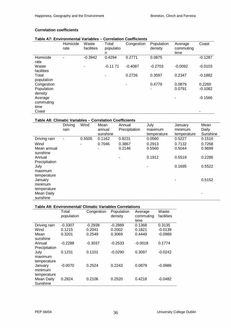
Happiness, Geography and the Environment Brereton, Clinch and Ferreira
PEP 06/04 University College Dublin 36
Correlation coefficients Table A7: Environmental Variables – Correlation Coe fficients Homicide
rate Waste facilities
Total population
Congestion Population density
Average commuting time
Coast
Homicide rate
- -0.3942 0.4294 0.2771 0.0875 -0.1287
Waste facilities
- -0.11 71 -0.4087 -0.2703 -0.0092 -0.0103
Total population
- 0.2726 0.3597 0.2347 -0.1882
Congestion - 0.4779 0.0879 0.2260 Population density
- 0.0791 -0.1082
Average commuting time
- -0.1566
Coast - Table A8: Climatic Variables – Correlation Coeffici ents Driving
rain Wind Mean
annual sunshine
Annual Precipitation
July maximum temperature
January minimum temperature
Mean Daily Sunshine
Driving rain - 0.5505 0.1162 0.8231 0.0560 0.5227 0.1516 Wind - 0.7046 0.3867 0.2913 0.7132 0.7268 Mean annual sunshine
- 0.2146 0.5560 0.5044 0.9699
Annual Precipitation
- 0.1912 0.5519 0.2286
July maximum temperature
- 0.1695 0.5522
January minimum temperature
- 0.5152
Mean Daily sunshine
-
Table A9: Environmental/ Climatic Variables Correla tions Total
population Congestion Population
density Average commuting time
Waste facilities
Driving rain -0.3307 -0.2938 -0.2889 0.1368 0.3135 Wind 0.1215 0.2041 0.2002 0.1821 -0.0139 Mean sunshine
0.3201 0.2549 0.3069 0.4449 -0.0989
Annual Precipitation
-0.2288 -0.3037 -0.2533 -0.0018 0.1774
July maximum temperature
0.1231 0.1101 -0.0290 0.3097 -0.0242
January minimum temperature
-0.0070 0.2524 0.2243 0.0879 -0.0986
Mean Daily Sunshine
0.2824 0.2106 0.2520 0.4218 -0.0482