Embed Size (px)
Citation preview
i
PLANNING AND SCHEDULING PROBLEMS IN
MANUFACTURING SYSTEMS WITH HIGH DEGREE OF
RESOURCE DEGRADATION
A Dissertation
Presented to
The Academic Faculty
by
Rakshita Agrawal
In Partial Fulfillment
of the Requirements for the Degree
Doctor of Philosophy in the
School of Chemical and Biomolecular Engineering
Georgia Institute of Technology
August, 2009

ii
PLANNING AND SCHEDULING PROBLEMS IN
MANUFACTURING SYSTEMS WITH HIGH DEGREE OF
RESOURCE DEGRADATION
Approved by:
Dr. Jay H. Lee, Advisor
School of Chemical and Biomolecular
Engineering
Georgia Institute of Technology
Dr. Hayriye Ayhan
School of Industrial and Systems
Engineering
Georgia Institute of Technology
Dr. Matthew J. Realff, Advisor
School of Chemical and Biomolecular
Engineering
Georgia Institute of Technology
Dr. Shabbir Ahmed
School of Industrial and Systems
Engineering
Georgia Institute of Technology
Dr. Dennis W. Hess
School of Chemical and Biomolecular
Engineering
Georgia Institute of Technology
Date Approved: [July 02, 2009]

iii
To my beloved grand parents and parents

iv
ACKNOWLEDGEMENTS
I wish to thank Dr. Jay Lee for his support and direction during my doctoral
studies. Many thanks to Dr. Matthew Realff for his support, vision and insight. His
methodical approach to problem solving and encouraging words always filled me with
optimism, energy and enthusiasm. I had the good fortune of working with Dr. Chad
Farschman, during two summer internships at Owens Corning. His leadership and
guidance made it a great learning experience for me.
I found a great friend and mentor in Nikolaos Pratikakis. I admire him for his
caring nature, cheerfulness and good humor. It was fun sharing the office space, ChBE
gossip and research ideas with (current and former) LIDCUS members. Thanks for help,
counsel and co-operation. I am also grateful to the student advisors at office of
international education, namely Greg Simkiss and Bryan Shealer for all help during my
stay.
I owe a large part of my little achievement to my fiancée, Raghav, who made the
bright moments last longer and provided me with strength and sanity in moments not so
cheerful. Thanks to him for being my anchor and for being so caring. I am grateful to all
the friends I made along the way, for making my stay in Atlanta so memorable. Finally,
thanks to my little brother and my parents for their undying support. I derived inspiration
from their sacrifice, encouragement from their faith, found happiness in their pride and
all my strength from their unconditional love.
v
TABLE OF CONTENTS
Page
ACKNOWLEDGEMENTS………………………………………………………………iv
LIST OF TABLES………………………………………….……………………………..x
LIST OF FIGURES………………………………………………………………………xi
SUMMARY…………………………………………………..…………………………xiv
CHAPTER
1 INTRODUCTION…………………………………………………………….. 1
1.1 Hierarchical Decision-making in Manufacturing……………………...…1
1.2 Resource Degradation and Related Decision-making………………... 3
1.3 Uncertainty and Observability……………………………………….. 5
1.4 Outlook………………………………………………………………. 7
2 OVERVIEW OF DEGRADATION MODELING AND DECISION-MAKING
UNDER UNCERTAINTY…...………………………………………………….10
2.1 Overview of Degradation Modeling, Inspection Strategies and Solution
Frameworks………………………………………………………….. 10
2.1.1 Inspection-oriented Quality Assurance Strategies……………...10
2.1.2 Diagnosis-oriented Sensor Distribution Strategies – Process
Improvement………………………………………………… 12
2.1.3 Existing Sensor Technology and Defect and Variance Propagation
Models………………………………………………………... 13
2.1.4 General Integrated Control and Optimization Framework……. 14
vi
2.1.5 Techniques for Solution……………………………………….. 15
2.2 Markov Decision Processes…………………………………………... 15
2.3 Partially Observed Markov Decision Processes……………………… 19
2.3.1 PERSEUS – an Approximate Solution Method………………...22
3 PLANNING AND SCHEDULING WITH PERISHABLE NON-STATIONARY
RESOURCES…………………………………………………………............. 25
3.1 Introduction…………………………………………………………... 25
3.2 Problem description through stone veneer supply chain…………….. 29
3.2.1 Modeling Resource Age……………………………………… 30
3.2.2 Demand Modeling…………………………………………… 31
3.2.3 Resource Replenishment Lead Time and Reorder Limit……. 32
3.3 Deterministic Problem –LP Formulation……………………………. 33
3.3.1 Deterministic Demand and Resource Life……………………. 33
3.4 Dealing with Stochastic Problems…………………………………… 37
3.4.1 Stochastic Demand Modeling…………………………………. 37
3.4.2 Modeling Stochastic Resource Life…………………………… 39
3.4.3 Solving the Stochastic Problem……………………………….. 40
3.4.4 Rolling Horizon Approach……………………………………. 42
3.5 The Decoupled Problem……………………………………………… 45
3.5.1 Resource Reorder……………………………………………… 45
3.5.2 Production Planning…………………………………………… 46
3.6 Numerical Results and Discussion…………………………………… 47
3.6.1 Parameter Values………………………………………………. 47
vii
3.6.2 Features………………………………………………………… 50
3.7 Conclusions…………………………………………………………… 57
4 AN APPROXIMATE DYNAMIC PROGRAMMING APPROACH TO
SOLVING PLANNING AND SCHEDULING PROBLEMS WITH
PERISHABLE RESOURCES………………………………………………..… 58
4.1 Inventory Planning under Inflationary or Recessionary Demand
Scenarios – an Illustration…………………………………………….. 59
4.2 Formulation of the Perishable Resource Problem as MDP………….. 65
4.2.1 MDP Formulation…………………………………………….. 65
4.2.2 A Heuristic to Obtain Resource Transition and Allocation
Decisions……………………………………………………...… 68
4.3 Solution of the MDP…………………………………………………. 71
4.3.1 Problem Size………………………………………………….. 71
4.3.2 An Approximate Dynamic Programming Algorithm…………. 73
4.3.3 Demand Modeling Revisited…………………………………. 79
4.3.4 Results and Discussion………………………………………. 83
4.4 Conclusions…………………………………………………………. 85
5 HANDLING DEFECT PROPAGATION IN SYSTEMS WITH STATIONARY
EQUIPMENT AND COSTLY JOB INSPECTION……………………………86
5.1 Introduction………………………………………………………….. 86
5.2 System Description…………………………………………………… 88
5.2.1 Modeling Machine Deterioration……………………………… 88
5.2.2 Defect Accumulation and Propagation……………………….. 90
viii
5.2.3 Objective……………………………………………………… 90
5.2.4 The Single Machine System………………………………….. 90
5.3 A Re-entrant Flow Example – Modeling and Solution…………….. 93
5.3.1 Description…………………………………………………… 93
5.3.2 Formulation as POMDP……………………………………… 96
5.3.3 Characterization of FOMDP Policy………………………… 100
5.4 A Hybrid Flow Example – Modeling and Solution………………… 102
5.4.1 System Description…………………………………………... 102
5.4.2 Formulation as POMDP……………………………………… 103
5.5 Discussion on Results and Policy…………………………………… 206
5.5.1 Performance Comparison……………………………………. 106
5.5.2 Empirical Findings and Conjecture………………………….. 109
5.5.3 Value Function Approximation………………………………..109
5.5.4 Decision-tree Analysis…………………………………………111
5.6 Conclusions………………………………………………………...…112
6 MILP BASED VALUE BACK-UPS FOR POMDPs WITH VERY LARGE OR
CONTINUOUS ACTION SPACES…………………………………………... 113
6.1 Introduction…...………………………………………………………113
6.2 Related Work………………………………………………………….114
6.3 Mathematical Programming Based Value Updates.…………………..116
6.3.1 Formulation of the Mathematical Program…… ……………….116
6.3.2 Computational Efficiency of the Mixed Integer Formulation….119
6.3.3 Implementation and Policy Determination ..…………………...121
ix
6.3.4 Problem Size v/s Computational Complexity.………………….122
6.4 Value Iteration around Post-decision Belief State…………………… .123
6.4.1 The Basic Idea………….……………………………………….123
6.4.2 Derivation of Basic Equations and Formulation of Math
Program…………………………………………………………126
6.4.3 Comparison with Value Updates around Pre-decision Belief
States……………………………….....……………………….. 129
6.5 Illustrative Examples………………………………………………… 130
6.5.1 POMDP with Continuous Actions…………………………….. 130
6.5.2 POMDP with Discrete but Large Action Space – A Network Flow
Example……………………………………………………….. 135
6.6 Conclusions………………….………………………………………...150
7 CONCLUSIONS AND CONTRIBUTIONS………………………………….. 152
7.1 Conclusions and Contributions…..…………………………….... 130
7.2 Future Work…………………………………………………….. 135
APPENDIX A: Theorem 1………………………………….……………………….. 156
APPENDIX B: Demonstration for monotone value function……………………….. 157
APPENDIX C: Demonstration for monotone policy……….……………………….. 161
REFERENCES………………………………………………………………………... 164
VITA………………………………………………………………………………….. 172
x
LIST OF TABLES
Page
Table 3.1: Parameter values for the perishable resource problem…………………….. 48
Table 3.2: Deviations from nominal demands for the Light and Dark products……… 49
Table 3.3: Problem features and their levels considered for analysis………………… 51
Table 3.4: Performance of solution approaches I,II and III for various levels of
uncertainty. Lead time in mold arrival is 3 in all the case…………………. 52
Table 4.1: Parameters and policies for the inflationary demand scenario…………..… 64
Table 4.2: Policies corresponding to approaches I and II, for the inflationary and
recessionary demand scenario……………………………………………… 64
Table 4.3: Parameter values for the perishable resource problem……………………... 72
Table 4.4: Deviations from nominal demand for the light and dark products………… 81
Table 4.5: Results from ADP and rolling horizon solution methods………………….. 84
Table 5.1: Parameter values………………………………………………………….... 107
Table 5.2: Results for the re-entrant and hybrid flow problems……………………..... 108
Table 6.1: Parameter values for the system with two-continuous actions………….…. 132
Table 6.2: Results for the problems with continuous actions……………………….… 135
Table 6.3: Parameter values for the network flow problems…………………………. 145
Table 6.4: Problem size and results for the network flow problems…………….……. 150
xi
LIST OF FIGURES
Page
Figure 2.1: Value iteration algorithm for solution of MDP……………………………. 18
Figure 3.1: Flow diagram for the bi-layer inventory control problem………………… 28
Figure 3.2: Demand patterns…………………………………………………………… 31
Figure 3.3: A seasonal demand scenario………………………………………………. 32
Figure 3.4: Time scales associated with the planning and scheduling problems considered
in this work…………………………………………………….................... 33
Figure 3.5: Deterministic initial age distribution of new resources……………………. 35
Figure 3.6: (a) Illustration of highly fluctuating stochastic demand pattern. (b)
Realizations of a highly fluctuating demand pattern……….......................... 38
Figure 3.7: (a) Seasonal demand pattern prone to uncertainty (b) Realizations of the
stochastic seasonal demand pattern………………………………………… 39
Figure 3.8: Flow diagram for the rolling horizon solution approach…………………… 44
Figure 3.9: Solution algorithm for the rolling horizon solution approach……………… 44
Figure 3.10: Flow diagram for the solution of the decoupled problem………………… 47
Figure 3.11: Results and comparison……………………………………………………. 56
Figure 4.1: (a)A demand model involving inflationary demand scenario (b) Illustration of
transition probabilities of the Markov chain.................................................. 61
Figure 4.2: (a) A demand model involving inflationary and recessionary demand
scenarios.(b) Illustration of transition probabilities of the Markov chain….. 62
Figure 4.3: Time scales of the planning and scheduling problems…………………….. 67
Figure 4.4: Heuristics……………………………………………………………………. 71
Figure 4.5: An approximate dynamic programming algorithm………………………… 78
xii
Figure 4.6: (a) number of states growing with iterations, (b) Convergence of value
function……………………………………………………………………… 80
Figure 4.7: Sample realization of switching mean (inflationary demand scenario)……. 83
Figure 5.1: (a) Serial production system with rework (b) Assembly system with scrap.. 89
Figure 5.2: Optimal policy for three-state single machine problem……………………. 93
Figure 5.3: Re-entrant flow problem…………………………………………………… 94
Figure 5.4: State transition for the re-entrant flow problem for 3 levels of machine
deterioration and L=3………………………………………………………. 98
Figure 5.5: Algorithm I for solving POMDP…………………………………….…… 101
Figure 5.6: Hybrid –flow system……………………………………………………… 103
Figure 5.7: Value function v/s linear approximation plot………………………………110
Figure 5.8: Algorithm II to solve POMDP with linear value function approximation… 111
Figure 5.9: Decision tree for the single machine problem……………………………... 112
Figure 6.1: (a) Value function calculation at a query point (b) Feasible region for the
MILP model for value update………………………………………………. 117
Figure 6.2: The MILP for determination of the maximizing action for value update….119
Figure 6.3: A schematic of pre-decision state to post-decision state and again to pre-
decision state……………………………………………………………….. 124
Figure 6.4: The MILP for determination of the maximizing action for value update for a
post-decision belief state………………………………………………….…128
Figure 6.5: Feasible region for the continuous two-action problem…………………. 132
Figure 6.6: Value function and policy comparison for two action system……………. 134
Figure 6.7: The comparison of convergence times and performance for the problem with
continuous actions…………………………………….................................. 137
Figure 6.8: A five-node network flow problem……………………………………… 139
Figure 6.9: MILP model for the value backup for network flow POMDP…………… 144
xiii
Figure 6.10: Illustration for mapping state l to l1……………………………………. 145
Figure 6.11: Cost parameter for the network flow problem with four, five and six
nodes……………………………………………………………………...... 146
Figure 6.12: Comparison between solution times of the MILP based backups and the
enumeration based backups for the network flow problem……………….. 148
Figure 6.13: Comparison between solution times of the MILP based backups and the
enumeration based backups for the network flow problem…………………149
xiv
SUMMARY
Mortality is the fundamental property of all matter. Various types of equipment
used in manufacturing industry are no exception. A machine, tool-group or piece of
equipment, jointly referred to a „resource‟ may deteriorate in many possible ways.
Depending on the form of degradation, preventive or corrective measures are employed.
The preventive measures such as machine maintenance, equipment/ process monitoring
etc. help keep the equipment functioning smoothly while corrective measures such as
replacement, repair etc. aim at minimizing disruptions in production due to resource
failure. In order to fulfill the production requirements, it is imperative that the resource
management decisions (including preventive and corrective decisions) be taken in an
optimal manner. More often than not, the resource management decisions are affected by
other production related decisions like production planning and scheduling, job
inspection, etc. The central theme of this thesis is to address the different ways in which
manufacturing resources deteriorate and develop optimization models for resource
management in conjunction with other production related decisions.
Oftentimes, specialized equipment, used in relatively large quantities on the
production floor are amenable to break frequently with use. The best example is a steel,
aluminum or plastic mold (also called a die) used for the manufacturing of a variety of
plastic goods, china, art work, machinery, electronics and building materials. After many
uses and cleaning, the mold tends to wear out, deform, or lose precision due to deposits.
Aside from a range of molds for products of different shapes and sizes, an inventory of
spare molds needs to be maintained. This repeated-use-limited-life feature is also found
in semi-conductor industry and printing industry in the form of masks and ink cartridges
respectively. Additional examples are seen in general manufacturing environments;
where expensive cutting tools, bushings, filtering equipment, spare parts etc. need
frequent replacement due to wear or clogging. This category of resources is collectively
referred to as perishable resources. In Chapter 3, the management of perishable resources
is considered together with production planning and resource allocation or production
xv
scheduling decisions. It is shown that these decisions are inter-dependent, and therefore,
call for a combined optimization problem.
This new class of problems is solved using the widely accepted framework of
hierarchical planning and scheduling using mathematical programming models. The
results of this approach are compared (on several avenues) with the solution of the
resource management problem when solved independent of production planning. A
rolling horizon methodology is employed when the parameters like product demand and
resource life have associated uncertainty.
However, when the system is plagued by high level of uncertainty, the
performance of the rolling horizon approach is often unsatisfactory. To resolve this issue,
the planning level problem is reformulated as a Markov decision process (MDP) in
Chapter 4 and solved using an approximate dynamic programming (ADP) algorithm. The
problem, in this form, resembles a popular class of problems called dynamic resource
allocation problems (Powell 2005). However, the additional decisions related to
production planning and resource procurement, introduce challenges in terms of problem
formulation and determination of state transition function. Compared with the rolling
horizon method, the ADP takes a more comprehensive view of the uncertainty, thereby,
giving improved performances in all the stochastic models that are considered.
The focus is then shifted to the more popular category of manufacturing
equipment, i.e., relatively bigger machines that are very costly to replace. The problem of
devising an optimal preventive maintenance strategy for a single machine deteriorating
randomly has been extensively studied (Monahan 1982). It is assumed that the machine
condition degrades progressively with use in a non-self-announcing manner. This implies
that the machine condition is not observed directly, but the degradation is reflected in
increased production of defective items or reduced product quality. Inspection of the
processed job, therefore, helps monitor the machine condition. But in the presence of
high inspection costs, job inspection also becomes a part of the decision-making. This
optimization problem has been successfully solved as a partially observable Markov
decision process (POMDP), owing to limited observability of the machine state.
xvi
When the aforementioned machine/resource becomes a part of the manufacturing
supply chain, it is bound to interact with other resources and possibly operate on multiple
types of jobs. These possibilities are addressed in Chapter 5, by considering two process
flow topologies: (i) re-entrant flow and (ii) a combination of re-entrant and serial flow
topology referred to as hybrid flow. Due to costly inspection, not every processed job is
tested. Consequently, the untested, potentially defective items move on to the next series
of operations, thereby getting accumulated in the system, until removed in final product
testing. The job inspection decision must now be taken to minimize this possibility in an
economically favorable manner. This quality-control aspect is the single-most interesting
addition to the optimization problem, together with the fact that, the resource
management decisions for multiple resources are inter-dependent. The combined
optimization problems for the two process flow topologies are solved as a (considerably
larger) POMDP. Recent developments in the area of POMDP solution methods
contribute greatly to the successful solution of the above problems. It is shown that the
rigorous method using POMDP formulation has a large potential for improvement over
heuristic rules.
Aside from machine maintenance, POMDPs have been successfully applied to a
variety of stochastic problems with partial information. Their applications range from
sensor allocation, robotics, network troubleshooting, moving target search etc
(Cassandra, 1998). For this reason, POMDPs have received significant attention in the
recent years (Spaan 2005; Thrun 2003; Simmons 2004). Since the exact solution methods
are limited to very small sized problems, most research efforts have been spent on
approximate solution methods. Approximate solution methods like point based methods,
seek to perform Bellman updates on a subset of the state space (called belief space in this
case). When the actions are continuous or have large number of dimensions (resulting in
very large action spaces due to combinatorial reasons), the value updates are performed
on a sampled set of actions. POMDPs with very large action spaces may also be solved
using policy graph or policy iteration methods, but such methods are prone to local
optima. In Chapter 6, an algorithm for the solution of POMDPs with high dimensional or
continuous action spaces is developed. The Bellman updates are performed using a mixed
integer linear program (MILP). MILP based Bellman updates can handle the continuous

xvii
or high dimensional actions while preserving the solution quality as opposed to the action
sampling methods. The MILP based methods also provide better scalability with problem
size. The concepts are illustrated by using a hypothetical POMDP with continuous
actions followed by a network flow example. The latter corresponds to the case of
discrete but high dimensional action space. The network flow problem also serves to
represent yet another category of resource management problems, where the nodes of the
network are prone to random contamination. This is a possibility in water, food and
computer networks. Electrical networks, on the other hand, are prone to random outages.
The network flow problem is solved using the existing enumeration based methods and
the new (MILP based) solution algorithm. A comparison of solution times and solution
quality are presented for both the examples.
In an alternative formulation, the MILP based Bellman updates are developed for
POMDP around post-decision belief states. Formulation around post-decision belief
states removes the dependence of MILP solution time on the size of the observation
space. This enables the algorithm to be applied to a wider spectrum of POMDPs.
Chapters 1 and 2 are aimed at familiarizing the reader with the basics of planning
and scheduling, resource degradation, inspection for diagnosis and quality control and
existing models and methods. By formulation of problems and development of solution
algorithms in Chapters 3 through 6, this thesis seeks to contribute an enhanced
understanding, novel problems and efficient solution methods to the existing body of
knowledge on (the general area of) resource management and related decision-making in
various process industries.
1
CHAPTER 1
INTRODUCTION
1.1 Hierarchical decision-making in manufacturing
In a typical manufacturing environment, a detailed planning process is adopted in
order to ensure the best utilization of resources and maximize a firm‟s profitability. This
is done in a hierarchical fashion due to differences in time-scales and the impact of
decisions constituting the planning process. (Anthony 1965) and later (Miller 2002)
provide details on the concept behind Hierarchical Production Planning (HPP). The
decisions are broadly classified into three categories.
Strategic planning:
At the strategic manufacturing planning level, the firm must address issues that
bear a long term impact. Such issues comprise of the total planned production capacity
levels for the next two, three, or more years; the number of facilities it plans to operate;
their locations; acquisition of manufacturing and storage capacities and procurement of
resources etc. Decisions made at the strategic production planning level place constraints
on the next level of decision making, i.e., tactical planning level.
Tactical planning:
At this level, the chief goal of the decision-maker is to obtain and use the
available resources effectively and efficiently. Typical planning activities include the
allocation of capacity to various products, planning workforce levels, logistics of
sourcing and distribution, preventive maintenance scheduling, and total quality
management. The use of existing infrastructure is maximized while staying within the
constraints of the firm‟s manufacturing and distribution infrastructure (as determined by
previous strategic decisions). As with the previous level of decision-making, the planning
decisions carried out at the tactical level impose constraints upon operational planning
and scheduling decisions as discussed further. Typical planning horizons are 12 -18
months.
2
Operational planning:
The routine decisions related to shop floor control fall under this category. At this
level, it is ensured that individual processes run efficiently and effectively. Master
production scheduling, labor scheduling, process improvement, inspection and repair,
truck load quantities, short term carrier selection etc. are a few examples of operational
planning decisions.
At the lowest level of decision-making, i.e., the operational planning and
scheduling level, most details about the individual processes are included. This leads to a
high degree of complexity although the decisions have a very short term impact. As we
move up the hierarchy, the system variables are aggregated. However, the risk associated
with the decisions and their impact rises as we go from operational to tactical level and
from tactical to strategic level. As noted in (Miller 2002) “A true HPP system is a closed
loop system which employs a “top down” planning approach complemented by “bottom
up” feedback loops. Given the emphasis of HPP systems on evaluating capacity levels
and imposing and/or communicating capacity constraints form higher levels down to
lower levels, it is imperative that strong feedback loops exist”. This is because at the
higher levels, possible infeasibilities are ignored or obscured due to aggregation. If the
information about these infeasibilities is not communicated back to the higher levels, the
firm may always function sub-optimally and may pay dearly. Together with strong
feedback loops, a judicious scheme for aggregation of information is needed to construct
the planning problems at various levels. This aspect often blurs the line between different
levels of decision-making and results in an interesting inter-play between decisions at
various levels. Particularly, in systems where there is a notable deterioration associated
with manufacturing equipment, the classification of decisions into various levels of
planning may present substantial challenges. Deterioration in manufacturing equipment is
discussed further.
3
1.2 Resource degradation and related decision-making
Although resource is a general term, it is used in this work to specifically refer to
a machine, equipment or tool group that facilitates production. In general, all
manufacturing equipment is prone to degradation with time. The features listed below
determine their impact on decisions related to manufacturing:
Type of degradation – The wear and tear associated with the usage of resource affects
its performance. The degradation is generally reflected in falling product yields in flow
type equipment, increased fraction of defective outcomes in discrete manufacturing
(termed as process drift), larger number of non-conforming batches in batch processing
etc. A complete failure or shutdown of the resource may also occur, leading to a halt in
production. Yet another form of degradation is contamination of the resource to render it
useless or even harmful for use. This is seen in network flow problems where the nodes
of the network that facilitate flow of materials or information, have finite probabilities of
contamination. Although, the nodes loosely fit the definition of a resource, it represents
an important class of degradation management problems. In general, the degradation is
caused by numerous factors including usage, age, type of operation, environmental
conditions etc.
Corrective or preventive action – In view of the above mentioned deterioration, a
preventive maintenance action needs to be taken to ensure equipment health. The
frequency of the preventive action is largely dependent on the time scales associated with
the degradation and trade-offs between the cost of maintenance and that of faulty
products. Corrective action in the form of inspection and repair is required on the faulty
outcomes. When the equipment breaks completely, it needs to be replaced or repaired.
The downtime may encourage keeping spare equipment/resources. The choice of
preventive and corrective actions is governed by industry, manufacturing process and
costs involved with maintenance, repair and replacement.
Time scales – The period of time for which the equipment goes without showing signs of
degradation is important to devise preventive and corrective actions. The time-scales
associated with degradation are typically measured as expected time to failure or time
4
until the process yield falls to x% of the best possible yield. If the time-scales are very
large, then the resource management decisions may be made independent of production
decisions. However, if the time-scales are comparable with that of production, then
resource failure or unavailability affects the production scheduling directly. In this case,
the downtime associated with resource repair or maintenance must be accounted for in
the production schedule.
Degradation dynamics – The dynamics associated with the degradation play an
important role in resource maintenance decisions. The resource may degrade in a
deterministic or stochastic manner. The variance associated with uncertain resource
lifespan may be large. This warrants a more conservative preventive maintenance plan.
Steep increases in defect fractions call for frequent product testing and resources prone to
sudden and untimely failures require the presence of spares.
Upstream and downstream processes – The resource management decisions may not
be taken independent of the rest of manufacturing supply chain. In general, the resources
at the beginning of the production sequence need to be monitored more closely. This
would avoid losses in terms of downtime during a failure and (or) propagation of faulty
jobs to downstream processes.
Possibility of detection – Direct inspection of the equipment may be performed as part
of routine check-up. When this is not possible or sufficient, inferential measurements on
product attributes are taken to monitor the performance of the equipment. In situations
where the quality is not reflected in process or control variables, installation of job-
specific inspection stations or sensor networks is required for product testing. When
equipment inspection or job inspection is costly, an inspection strategy becomes a part of
the decision-making as well.
The knowledge of above factors is central to devising an efficient resource
management plan and to establish whether resource management needs to be done in
unison with other manufacturing related decisions like production planning and quality
testing. As noted in above discussion, the resource failure rates may have associated
uncertainty. This, together with other sources of uncertainty, poses challenges in
5
modeling and solution. The other sources of uncertainty and a brief discussion on
solution methods are covered in the following section.
1.3 Uncertainty and observability
At different levels of the decision-making hierarchy, uncertainties present
themselves in various forms. The presence of uncertainty results in several possible
outcomes and future system states, often having far-reaching effects. Depending on the
level and form of the uncertainty, it becomes imperative to factor it into the decision-
making. This is because extreme realizations of uncertainty may result in great loss of
performance, operational infeasibility or both. Uncertainty in the realm of planning
problems may be classified as below:
Parametric uncertainty – When the problem parameters have randomness associated
with them, the uncertainty is external to the system. The exogenous information about the
parameters becomes available after the relevant decisions have been made. For example,
the product demand for a firm‟s products is often uncertain and a buffer stock or safety
stock is maintained to counter the effect of uncertainty. If the available stock falls short of
extremely high realizations of demand, the stock-outs lead to loss of potential revenue
and hamper the firm‟s reputation. Other examples of parametric uncertainty include
market price for products, raw materials, utilities etc., raw material quality, conversion
rates,
Decision Uncertainty – Often the outcome of a decision cannot be known with complete
certainty because of the uncertainties associated with the process. For example, a decision
is made to produce x units at a particular machine in a given time frame. However, due to
random failure, only x-y, y>0 units could be made. In a different scenario, x units are
decided to be manufactured by assuming an expected process yield of beta. This implies
that a fraction of produced units will be found non-conforming by appropriate quality
standards. However, a higher realization of beta results in lower number of conforming
units. Robot movement, production throughput, corrective or repair actions, order
quantities, sensor failure are a few more examples of decision uncertainty.
6
State uncertainty - When the elements of the state of the system are not known with
complete certainty, a probability distribution is maintained over the state. In control
applications, state uncertainty is generally attributed to measurement noise and an
estimate of the state is maintained. In planning frameworks, the presence of this type of
uncertainty is referred to as partial observability. For example, in a retail store, the
inventory of products in the store is seldom known with certainty. Partial observability of
the state is also a concern in preventive maintenance planning where the deterioration
level of equipment is not completely observed. Errors associated with measurement
sensors also leads to randomness in state estimates.
There is a fine line between the first two types of uncertainties in that they affect
the future state in similar manners and the realization of uncertainty becomes available
after an action is taken, i.e., the parameter values are realized or the effect of action
becomes known. Therefore, both the parametric and decision uncertainties can be
accounted for by similar modeling and optimization methods. However, in the case of
state uncertainty, the realization of system‟s true state may never become available.
Therefore, using the term uncertainty is a misnomer and it will be referred to as partial
observability of state for future analysis. Specialized algorithms have been developed to
solve optimization problems with partial state information.
Several techniques exist for solving general stochastic optimization problems:
Stochastic dynamic programming (Bellman 1956; Puterman 1994).
Mathematical programming methods like stochastic programming (Andrzej and
Ruszczyński, 2003) and robust optimization.
Simulation methods like simulated annealing (Kirkpatrick and Vecchi, 1983),
genetic algorithms (Schmitt 2001) or Monte Carlo (Fishman 1996) simulation.
The applicability is largely governed by problem size, problem type (discrete or
continuous states and actions) and search complexity. Most of the above methods
optimize the expected value of the objective. Robust optimization considers the worst
7
case uncertainty by using a min-max approach while certain formulations like value at
risk (var) or conditional value at risk (covar) also account for variance in the objective.
1.4 Outlook
As described in section 1.2, depending on the extent and type of resource
degradation, other manufacturing decisions need to be taken in conjunction with the
resource management decisions. For this purpose, three broad categories of resources are
considered. The first category consists of small pieces of equipment that are present in
large quantities on the production floor, and may move from one operation to the other.
In the course of manufacturing, these resources are amenable to breaking (perishable
resources), getting consumed (expendable resources) or exiting the system in some other
way. Examples of such resources includes small fixtures of machines like masks, lenses
in precision equipment manufacturing, substrates in catalysis, molds in building material
industry, ink cartridge in printing industry etc. Human resources fall in this category
when the employee turnover rates are high. This is true of industries like construction,
military, call centers and consulting. The unique feature that differentiates the above from
raw materials is that the resources can be employed multiple times before they exit the
system. Since resources belonging to this category are generally required in relatively
large quantities and the demand for them may not be well understood, an inventory is
usually maintained. The demand for resources is determined by the production
requirement and therefore, the inventory control at the product and resource levels
becomes coupled. This problem can be viewed as a nested inventory control problem and
is addressed in Chapter 3. In Chapter 3, mathematical programming models are
developed for decision-making at planning and scheduling levels in a hierarchical
fashion. Parametric uncertainty is handled by solving the planning and scheduling
problem in a moving horizon fashion.
Depending on the its form, a myopic view of the uncertainty taken by the rolling
horizon solution approach may not be very effective. For this reason, an approximate
dynamic programming (ADP) algorithm is implemented to solve the perishable resource
8
inventory control in conjunction with production decisions. The solution from ADP is
compared with that of the rolling horizon method.
The second category comprises the large machines which deteriorate gradually so
that preventive maintenance needs to be performed on the machine/ resource from time to
time. However, the degradation is prone to uncertainty and is seldom observed directly.
Inferential measurements in the form of the quality of processed job are often taken to
access the state of the machine. However, when product inspection is costly, it may not
be economically favorable to test all the processed jobs and job inspection becomes a part
of the decision-making. In a manufacturing system with multiple operations, the untested
jobs move downstream for further processing. In the event that an untested job does not
satisfy the quality requirements, this would result in propagation of defects, thereby
raising quality control issues. This feature of defect propagation is addressed in Chapter 5
by means of two process flow topologies: (i) a re-entrant flow system and (ii) a hybrid
flow system, in a discrete/batch manufacturing system. Due to lack of full information
about the system at all times, e.g., the machine state, the problem is formulated and
solved as a partially observed Markov decision process (POMDP). A comparison with
alternative solution methods and an analysis of the solution properties is presented.
Over the last decade, considerable research efforts have been spent in the area of
developing efficient algorithms to solve POMDPs. Since exact solution methods are
limited to very small problem sizes, the focus is mainly on approximate solution
methods. However, literature is relatively sparse on POMDPs with very large or
continuous state, action and observation spaces. To this end, a mixed integer linear
programming (MILP) based solution algorithm is developed in Chapter 6. In an
alternative formulation, the POMDP solution is structured around the post-decision state
variable to limit the effects of a large observation space. The methodology is
implemented on a network flow problem, which comprises the third category of
resources prone to degradation.
A network comprises of nodes and edges that facilitate the flow of material like
water, food, electricity etc. or information like computer network or supply chain
network etc. Occasionally, the nodes of the network get contaminated and the

9
contamination is amenable to spread to the downstream node. It is therefore imperative to
track down and repair the contaminated/corrupted node and divert any flows so as not to
pass through it. This problem is also formulated and solved as a POMDP using the MILP
based algorithm. The solution quality and convergence times are compared with those of
the traditional method.
10
CHAPTER 2
OVERVIEW OF DEGRADATION MODELING AND DECISION-
MAKING UNDER UNCERTAINTY
2.1 Overview of degradation modeling, inspection strategies and solution
frameworks
Degradation of manufacturing equipment/resources can manifest itself in many
different ways. For example, with age or deterioration, the equipment might increasingly
produce lower quality products, may cease to work, may corrode downstream equipment
etc. A particular type of degradation of interest is when the gradual degradation of
production equipment is reflected in increased production of off-specification products.
In this case, the detection of quality attributes of the products requires job inspection by
means of measurement sensors. Literature is replete with studies on inspection allocation
in manufacturing environments. Along with degradation management, much of the work
in the past has gone into detecting the degradation by means of correct inspection
strategy. Serial manufacturing systems have been most popular means of illustration of
the concepts. A serial manufacturing line has sequential operations and the product flow
is linear. The sensor allocation is performed with one of the two major objectives;
namely, inspection oriented quality assurance policies that are aimed at product
improvement by rework/ repair and the diagnosis- oriented sensor distribution strategies
which are focused on diagnosing the deteriorating process/equipment. The two broad
problem classes are discussed in further details.
2.1.1 Inspection-oriented quality assurance strategies
The inspection-oriented quality assurance strategies may be viewed as a
corrective measure to ensure that the faulty products do not reach the end customers.
These account for the trade-offs between the costs associated with inspection stations and
the returns obtained by the improved quality of processed jobs. Some of the early works
in this area are reported in (Raz 1986). Most of the authors that were cited, consider serial
11
manufacturing lines for inspection allocation due to ease of analysis. The literature on
inspection allocation problems, since then, is comprehensively reviewed in (Mandroli et
al, 2006). A typical serial production line has single or multiple types of jobs, all with a
predetermined sequence of operations. The allocation problem entails determining the
optimal locations of inspection stations when there is limited inspection capacity.
Inspection capability may also be limited by cost being substantial if it was to occur after
every operation. The defect level found upon inspection can be a binary or continuous
measure, and different decisions like rework repair, replace or scrap are taken depending
on the production stage and extent of defect. The intensity of inspection, e.g. selective
inspection and repeated inspection is also a decision to be considered. The inspection
may be prone to imperfections and may have type I or type II errors as explained below:
(i) the wrong rejection of a conforming unit (type I error)
(ii) the erroneous acceptance of a non-conforming unit (type II error)
The jobs may have multiple defect types as caused by different operations. The
inspection stations may or may not be able to detect all defect types caused in the past. In
the absence of the ability to detect all types of defects, the inspection is termed
specialized. A sub-set of above mentioned issues have been considered in literature,
which is briefly reported here.
Earliest work in this area was conducted by (Lindsay and Bishop, 1964) who
formulated a dynamic programming problem for basic issues related with inspection
allocation. They also proved that an extreme point solution (0% or 100 %) is optimal, if it
is assumed that all rejected items were scrapped, unless we have a constraint on final
product quality level. The extreme point solution boils down to inspecting all jobs
whenever an inspection station exists after an operation. A screening inspection program
for a multistage process can be established by considering three related decisions. These
include the location of inspection station, the level of inspection at each inspection point
and types of inspection at any stage for specialized inspection stations. This concept of
specialized inspection problem was further extended by (Rebello et al, 1995) who
presented some exact and heuristic solution methods. (Lee and Unnikrishnan, 1998)
12
extended the above mentioned decision making to multiple part types which have
different sequences of operation. They also relaxed the perfect inspection assumptions
made by the above mentioned works and included inspection errors. Shiau (2003)
assigned dynamic tolerances for inspection, by assuming a random defect generation
model, and proposed heuristics for solution of the resulting large size problem. Kakade et
al, (2004) proposed a simulated annealing approach to capture economic tradeoffs
between product yield and inspection accuracy. Gurnani et al, (1996) integrated the
inspection allocation problem with that of capacity planning and inventory levels.
Another aspect of inspection allocation is dedicated to equipment diagnosis and process
improvement. This aspect is discussed in the following section.
2.1.2 Diagnosis-oriented sensor distribution strategies – Process improvement
To facilitate process improvement or maintenance scheduling, sensor distribution
strategies must have a deeper insight into the measurements of faults and defects. The
process variables and quality variables that provide the information about machine health
are the target of this study. The decisions involved in this type of study are
(i) The workstations where to place the sensors
(ii) The physical variable to be measured at each station
(iii) Equipment maintenance decisions – service or replace the machine
Mandroli et al, (2006) reviewed existing literature on quality-fault modeling and
effectiveness of sensor systems. For optimal allocation in this case, a measure of
effectiveness is maximized, the overall cost is minimized or yield is maximized with
constraints on sensor allocation. Optimization approaches like Powell‟s direct search
(Wang and Nagarkar, 1999), sequential quadratic programming or gradient-based search
(Khan et al, 1999), exchange algorithms (Liu et al, 2005), have been used in the existing
literature. Nurani el al, (1994) developed an optimal sampling plan specifically in semi-
conductor fab using a statistical process control approach.
The sensor allocation is followed by machine/ process improvement. To this end,
Rabinowitz and Emmons, (1997) proposed a setting where defects provide full
13
information about health of the machine and machine is repaired whenever it is detected
to be malfunctioning. Expanding the work, Emmons and Rabinowitz, (2003), the authors
proposed heuristics methods for inspection task scheduling in general deteriorating
systems. Bowling et al, (2004) prescribed optimum process targets using a Markovian
approach, while Yacout and Gautreau, (2000) included partial observability in their
analysis. Yao et al, (2004); Marcus et al, (2004) considered the impact of production
constraints on preventive maintenance (PM) scheduling in manufacturing systems. They
developed a hierarchical method to obtain a time window within which PM must be
scheduled. Cassady and Kutanoglu, (2005) integrated PM scheduling and production
scheduling in an MILP framework.
2.1.3 Existing sensor technology and defect and variance propagation models
To be able to mathematically analyze the system, we need to model the defect
generation by various operating stations/ machines. The model should be able to capture
the propagation of defect in multi-stage setting and sources of variations at a particular
station. Also, for process improvement and sensor distribution, appropriate process
variables must be included in the model. Cochran and Erol, (2001) proposed analytical
methods to model process flows, and performance measures like outgoing quality level
and throughput rate. Zantek et al, (2002) established modeling techniques for correlated
stages and estimated the parameter values by least squares method. Chan and Spedding,
(2001) captured the propagation of defectives by design of experiments (DoE), response
surface plot and a neural network model. State-space models have been frequently used
to characterize the variance (Ding et al, 2000; Huang and Shi, 2004). Huang and Shi,
(2004) used a state-space model to capture the propagation of variance in serial-parallel
multistage systems. To detect the source of variance in processes, Lee and Apley, (2004)
used linear structure model to generically represent the variation patterns. Batson (2004)
described a simple probabilistic model that describes the serial effects on the processed
parts. The cost of less-than perfect quality was approximated by a quadratic loss function
called Taguchi loss function.
To determine target applications for our methods, we reviewed the status of
sensor technology in a discrete part manufacturing setting, for example, semi-conductor

14
manufacturing. Grochowski et al, (1997) summarized the current status and trends in
integrated circuit testing. Kumar et al, (2006) reviewed the various yield modeling
techniques specifically in semiconductor manufacturing. Xiong et al, (2002) successfully
applied the modeling techniques for variation prediction in automotive assembling.
2.1.4 General integrated control and optimization framework
Given all these different aspects of decision making for inspection allocation and
process improvement, there is a need to integrate them into a single decision making
framework for optimal decisions. One example of such a framework is the fab-wide
control framework developed for semiconductor manufacturing processes (Qin et al,
2006). The authors used a hierarchical framework for integrated control. In the fab-wide
framework that they proposed, at the bottom of the hierarchy lie the run-to-run controllers
which optimize the local processing steps. These run-to-run controllers are controlled by
an „island of control‟ which in turn is supervised by an overall fab-wide controller
satisfying the economic goals. A similar integrated control framework was suggested by
Tosukhowong (2006) for continuous flow process plants. Similar methodology was
adopted by Vargas-Villamil et al, (2003), where use of Model Predictive Control (MPC)
is made at the intermediate layer. Sethi and Zhang, (1994) discuss hierarchical decision
making in stochastic manufacturing systems which brings together optimal control of
parallel machine and dynamic flow shops. Very few attempts have been made at using
frameworks that are different from hierarchical control frameworks. One such work
(Heragu et al, 2002) proposes an intelligent agent based framework which is a hybrid of
the hierarchical and heterarchical frameworks. They used the concept of holonic
structures that accomplish individual as well as system wide objectives. Inman et al,
(2003) considered the intersection of quality and production system design and suggested
new research issues regarding trade-offs between productivity, flexibility and quality in
manufacturing environment.
2.1.5 Techniques for solution
Since most of the above problems are multistage, Dynamic Programming (DP)
has been widely used as a solution approach for these problems (Lindsay and Bishop,
15
1964; Gurnani et al, 1996). Bertsekas (1995); Sutton and Barto, (1998) contain
comprehensive discussion on exact and approximate solution methods of the DP
problem. Many of the above problems can be formulated as Markov Decision Processes
(MDPs) in which transition between states follows Markov property. Quantitatively, this
is a „memory-less‟ property where system state and stage-wise reward only depend on the
one step prior state and action. Occasionally, the system state information is
missing/hidden causing it to be a Partially Observable Markov Decision Process
(POMDP). Other than DP, mixed-integer programming (MIP) and non-linear
programming (NLP) formulations have been successfully used in inspection allocation
problems (Rebello et al, 1995). Several heuristic methods like simulated annealing,
genetic algorithms, random search methods and simulation are used when problem size is
big enough to inhibit usage of exact solution methods. Some of the properties that
heuristics (rules of thumb) must capture are as summarized in Lee and Unnikrishnan,
(1998):
Inspect before costly operations so that these operations will not be performed on
non-conforming items
Inspect before items that cover up/obscure non-conformities
Inspect before operations where faulty items may jam or break the machines
Since MDP and POMDP have proven to be successful frameworks for solving
problems related to inspection, maintenance and production scheduling, the two
frameworks are reviewed in greater detail.
2.2 Markov decision processes
Markov Decision Processes (MDPs) provide a framework for modeling real world
processes which have a stage-wise structure. The stage can denote a time epoch or other
quantities like location, processing step etc. At any stage, the system is recognized as
being in a state (designated as s) which is a set of attributes that aid decision-making. The
set of all possible states is called state space (designated as S). Starting in state s S, there
16
is a set of actions from which the decision-maker must choose. The set of all possible
actions is called action space (A) and an element of the action space is denoted by a.
When action a is taken in state s, and the system transitions to the next stage, it ends up in
a unique next state s′ S in the absence of any uncertainty. However for stochastic
problems, there is a set of possible next states for each state-action pair. The probability
of transition to a particular next state, in this case, is governed by a state transition
probability function T. In the process, reward r(s,a,s′) is received, which is determined by
the reward function R. The dependence of r on s′ is often suppressed by taking a
weighted average over all possible states at the next stage. At each stage, actions are
taken so that the sum of stage-wise rewards is maximized. In the presence of uncertainty,
the expected sum of rewards is maximized. When infinite stages are present, i.e.,
extremely large time horizon, the future rewards are often discounted using a discount
factor γ. When the number of stages is infinite, the problem is called an infinite horizon
MDP as opposed to finite horizon MDP for finite number of stages. In most applications,
a stage symbolizes a time epoch. Therefore, we use the term time epoch or time step
synonymously with „stage‟ for future reference.
0
0
( ) [ ( , ( )) | ]t
t t
t
V s E r s s s s (2.1)
More formally, a MDP corresponds to a tuple (S, A, T, R, γ) where S is a set of
states, A is a set of actions, T : S×A×S→[0,1] is a set of transition probabilities that
describe the dynamic behavior of the modeled environment, R: S×A×S→ R denotes a
reward model that determines the stage-wise reward when action a is taken in state s
leading to next state s′ and γ→[0,1] is the discount factor used to discount future rewards.
A γ value close to 0, places very little weight on future rewards, while γ close to 1 results
in very little discounting.
The notational convention for MDPs is adopted from Hauskretch (2000) with
small modification. For ease of illustration symbol p(.) is used to denote probability of a
quantity and r(.) is used to denote reward (generally as a function of state and action). pij
signifying transition from state s=i to s′=j is used to denote transition probabilities
17
associated with the Markov chain. Ta is used to denote the probability transition matrix
corresponding to action a. Symbols s, s′ and a are used to denote current state, next state
and action and belong to sets S,S and A respectively.
One of the fundamental properties of the MDPs is that the transition and reward
functions associated with the stage-wise transition of state are independent of the past
states and actions. Referred to as Markov property, this memory-less feature enables the
decomposition of the overall optimization problem into separate stage-wise problems.
This is accomplished by using a recursive relationship between the value of being in a
state at any stage.
The goal is to maximize the (often discounted) sum of rewards over a time
horizon which can be either finite or infinite (2.1), where t denotes the time epoch, st is
the state at time t and π: S→A, is the policy that dictates the choice of action at time t.
This is achieved by solving the Bellman equation (Bellman 1956) for finite or infinite
horizon problems (2.2). It is well-known (Puterman 1994) that for infinite horizon
problems, a stationary optimal policy of the form in (2.3) exists, where V*(s) is the
average discounted infinite horizon reward obtained when the optimal policy is followed
starting from s until infinity (Puterman 1994). This implies that the state to action
mapping, in the form of optimal policy is independent of the time epoch. The existence of
stationary optimal policy is conditioned on the properties of model elements. One of the
sufficient conditions is that there be a finite action space As corresponding to each state
s S, maximum attainable stage-wise reward is finite and discount factor γ [0,1) . For all
applications in this work, the set of conditions noted here are satisfied. The alternative
sets of sufficient conditions for existence of a stationary optimal policy for discounted
infinite horizon MDPs can be found in Puterman (1994). In (2.3), a*(s) is the optimal
action to be taken when the system is in state s, independent of time t. V*(s) is called the
optimal value function and is obtained as the solution to Bellman equations (2.2) for all s.
SsAa
ssVasspasrsV'
** )}'(),|'(),({max)( (2.2)
18
SsAa
ssVasspasrsa'
** )}'(),|'(),({maxarg)( (2.3)
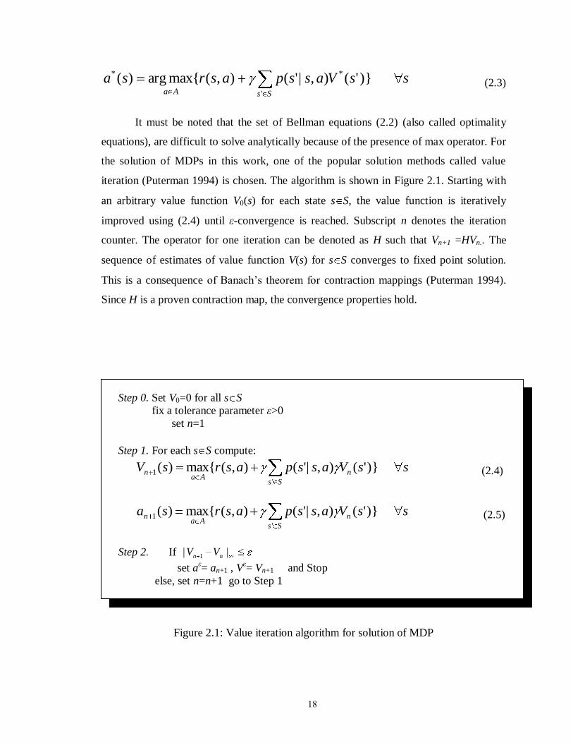
It must be noted that the set of Bellman equations (2.2) (also called optimality
equations), are difficult to solve analytically because of the presence of max operator. For
the solution of MDPs in this work, one of the popular solution methods called value
iteration (Puterman 1994) is chosen. The algorithm is shown in Figure 2.1. Starting with
an arbitrary value function V0(s) for each state s S, the value function is iteratively
improved using (2.4) until ε-convergence is reached. Subscript n denotes the iteration
counter. The operator for one iteration can be denoted as H such that Vn+1 =HVn.. The
sequence of estimates of value function V(s) for s S converges to fixed point solution.
This is a consequence of Banach‟s theorem for contraction mappings (Puterman 1994).
Since H is a proven contraction map, the convergence properties hold.
Step 0. Set V0=0 for all s S
fix a tolerance parameter ε>0
set n=1
Step 1. For each s S compute:
Ss
nAa
n ssVasspasrsV'
1 )}'(),|'(),({max)( (2.4)
Ss
nAa
n ssVasspasrsa'
1 )}'(),|'(),({max)( (2.5)
Step 2. If || 1 nn VV
set aε= an+1 , V
ε= Vn+1 and Stop
else, set n=n+1 go to Step 1
Figure 2.1: Value iteration algorithm for solution of MDP
19
Due to ease of implementation, value iteration is perhaps the most widely used
algorithm in dynamic programming. Certain other methods like policy iteration
(Bertsekas 1995), a hybrid between value iteration and policy iteration (Powell 2007) and
linear programming method for dynamic programs (De Farias and Roy 2003) are also
used depending on the problem structure. The complexity of the algorithm shown in
Figure 2.1 grows as a function of o(|S|2|A|). This is attributed to the three curses of
dimensionality noted below:
1. Equation (2.4) needs to be solved for all s belong to S, so the solution time is
directly proportional to |S|
2. The complexity of max operation depends on the size of the action space |A|
3. The calculation of expectation within the max operator depends on the number of
possible next states, i.e., |S|.
In the presence of large state and (or) action spaces, the value iteration algorithm
cannot be implemented in its exact form. Several approximation methods have been
developed to circumvent this difficulty. Some of them being, approximate dynamic
programming methods using value function approximations (Powell 2007), Q-learning,
temporal difference learning (Barto et al, 1995; Sutton and Barto, 1998), linear
programming methods using basis functions (De Farias and Roy, 2003) and dynamic
programming methods using post decisions state (Powell 2007). Details of particular
approximate solution methods used in this work are deferred until the specific
illustrations/applications for better understanding. All the above methods assume that the
system state is completely known or observed at all times. When this assumption does
not hold, the equivalent framework is called a partially observed Markov decision
process (POMDP) as discussed in the next section.
2.3 Partially observed Markov decision processes ( POMDP)
POMDP is a discrete-time stochastic control process when the states of the
environment are partially observed. Similar to the MDP, at any time, the system is in one
of the states s in the state space S. By taking an action a, the system transitions to the next
state s′ S according to known system dynamics p(s′|s,a) and accrues a reward r(s,a). The
20
next state s′ is not completely observed but an observation o may be made which is
probabilistically related to the state s′ and action a by p(o|s′,a).
More formally, it corresponds to a tuple (S, A, Θ, T, O, R) where S,A,T,R and γ
represent the same entities as described in section 2.2 on MDPs; Θ is a set of
observations, and O : S×A× Θ→[0,1] is a set of observation probabilities that describe the
relationship among observations, states and actions. The notational convention for
POMDPs is also adopted from (Hauskretch 2000) for consistency. Symbol o Θ is used
to denote an element of the observation space Θ.
When the system state s is not perfectly observed, a history of all actions and
observations (since t=0) need to be maintained. Due to the Markov property, this
information is contained in the probability distribution over all states at any time. The
probability distribution is referred to as belief state b(s) for s S. The belief states are
continuous since they contain the probability values, which are continuous numbers
between 0 and 1. Partial observability, thus converts the original problem into a fully
observable MDP (FOMDP) with continuous states. Since all the elements of a belief state
must add up to 1, the state dimension of FOMDP is one less than the size of the original
state space.
Similar to MDP, an infinite horizon POMDP has an optimal stationary policy
π* : Δ→ A which maps the belief states to optimal actions (Smallwood and Sondik,
1973). Δ :R|S|-1
(0,1) is the belief simplex containing all possible belief states. A policy π
can be characterized by a value function Vπ which is defined as the expected future
discounted reward. Vπ(b) is accrued when the system is initially in state b and policy π is
followed (2.6), where 10 is the discount rate that discounts the future rewards.
0
0
( ) [ ( , ( )) | ]t
t t
t
V b E r b b b b (2.6)
The value function corresponding to the optimal policy maximizes V(b) and satisfies the
Bellman equation (2.7) for all b.
Ss Oo
o
aAa
bVbaopsbasrbV )](),|()(),([max)( ** (2.7)
21
where, o
ab is the belief state obtained when action a is taken in state b and observation o
is made. The expression for o
ab is shown in (2.8).
),|(
)(),|'(),'|(
)'(abop
sbasspasop
sb Sso
a (2.8)
Similar to the value iteration for MDPs, the value update step for a belief point b is
shown in (2.9).
Ss Oo
o
anAa
n bVbaopsbasrbV )](),|()(),([max)(1 (2.9)
However, exact value iteration may not be performed due to the presence of
continuous states and consequently, infinite number of belief states. To alleviate this
problem, researchers have looked into ways to exploit the fact that the optimal value
function corresponding to POMDPs has a parametric form. For finite horizon problems,
the value function is piece-wise linear and convex (PWLC) (Smallwood and Sondik,
1973) and for discounted infinite horizon POMDPs, it can be approximated well with a
PWLC function (Sondik 1978).
The POMDP solution methods can be broadly classified into the following
categories (Hauskretch 2000; Spaan and Vlassis, 2005):
1. Exact solution methods:
Exact methods of solution of POMDPs were developed in 1970s and are still
being improved. Notable among these are enumeration (of all possible linear
functions) and pruning (Sondik 1978; Monahan 1982; Cassandra et al, 1997;
Zhang and Lee, 1998; Zhang and Liu, 1997). Sondik‟s one and two-pass
algorithms (Sondik 1978) and the Witness algorithm (Kaelbling et al, 1999; Littman
et al, 1995; Cassandra 1998).
However, the exact solution methods are limited to very small size problems.
(Papadimitriou and Tsitsiklis,1987) demonstrate that solving a POMDP problem
is an intrinsically hard task. Finding the optimal solution for the finite-horizon
22
problem is PSPACE-hard and finding the optimal solution for the discounted
infinite horizon criterion is even harder. The corresponding decision problem has
been shown to be undecidable (Madani et al, 1999), and thus the optimal solution
may not be computable.
2. Heuristic methods for value function approximation:
Several methods have been proposed for approximation of the value function
corresponding to the POMDP, e.g., approximation using the MDP value function
(Astrom 1965; Lovejoy 1993), approximation using MDP Q-function (Littman et
al, 1995) the fast informed bound Method (Hauskretch 2000), grid based
approximations using interpolation by convex rules or curve fitting.
3. Finite state controllers or policy graph methods (Kaelbling et al., 1999; Littman
1996; Cassandra 1998)
4. Point based methods.
Over the years, many methods have been developed that make use of the PWLC
structure of the value function to solve the POMDPs. Since, the exact solution methods
are limited to problems of very small sizes, approximate point based solution methods
like PERSEUS (Spaan and Vlassis, 2005), HSVI (Smith and Simmons, 2004), BPVI
(Pineau et al, 2003) etc. have been studied recently, which expand the scope of POMDPs
to problems of much larger sizes. PERSEUS is one of these methods, which uses the
concept of asynchronous dynamic programming and randomly updates only a subset of
belief states in one value iteration step. In this work, value updates in spirit similar to
PERSEUS are used. The algorithm is described in further detail below.
2.3.1 PERSEUS – an approximate solution method (Spaan and Vlassis, 2005)
Given the PWLC structure of the value function, the value function at the nth
iteration (Vn) is parameterized by a finite set of gradient vectors i
n , i= 1, 2, .., |Vn| (2.10).
The gradient vector that maximizes the value at a belief state b (also referred to as a
23
belief point or just point) in the infinite belief space is represented by )(b
n in (2.11).
Superscript i indicates the ith gradient vector in the set and superscript (b) indicates the
vector that maximizes Vn(b) for a particular b. During an exact value iteration step then,
the value (Vn+1(b)) and the gradient ()(
1
b
n ) corresponding to any point can be updated
using the Bellman backup operator as shown in (2.12) through (2.14).
i
nn bbVin
.max)( (2.10)
i
n
b
n bin
.maxarg)( (2.11)
b
ag
b
n gbbbackupAa
ba }{
)(
1 maxarg)( (2.12)
where,
i
oa
Ss o g
b
a gbsbasrgi
ioa
,}{ ,
maxarg)(),( (2.13)
Ss
i
n
i
oa sasspasopsg'
, )'(),|'(),'|()( (2.14)
BbbHVbVbV nnn )()()( 1 (2.15)
In PERSEUS, a subset B of belief points is obtained by taking random actions.
This belief set is fixed and chosen as the new belief space for value function updates. Due
to parameterization of the value function (2.10), an updated gradient vector for a belief
point may improve the value of many other points in the belief set. This leads to the
concept of approximate PERSEUS backups as shown in the algorithm below. Due to this
approximate update, in each value backup stage, the value of all points in the belief set
can be improved by updating the value and gradient of only a subset of points. The
resulting value function estimate will follow the condition shown in (2.15) where HVn is
the estimate, if the entire belief space were updated.
24
Perseus backup stage: Vn+1 = HperseusVn
1. Set Vn+1 = ø. Initialize to B
2. Sample a belief point b uniformly at random from B and compute α = backup(b)
3. If b.α ≥Vn(b) then add α to Vn+1, otherwise add i
nbi
in
.maxarg'}{
to Vn+1.
4. Compute = {b B: Vn+1(b) < Vn(b)}.
5. If = ø then stop, else go to 2.
PERSEUS is an elegant and fast method for solution of POMDPs with proven
convergence properties. For convergence, it is required that the initial value function is
always under-estimated everywhere. However, there are no performance guarantees with
respect to the optimal value function. This is because the method considers a randomly
selected belief set on which value iteration updates are carried out. This is done under the
assumption that the parameterization using the gradient vectors would generalize well to
the entire belief space. However, there is no indication of how good that generalization
will be, even after the convergence criterion is met. Therefore, re-sampling techniques
are used to ensure that the value function generalizes well to different parts of the belief
space.
With the basic understanding of related literature on formulation and solution of
manufacturing related problems in the face of resource degradation, a planning and
scheduling problem with non-stationary resources is presented in the following two
chapters.
25
CHAPTER 3
PLANNING AND SCHEDULING WITH PERISHABLE NON-
STATIONARY RESOURCES
3.1. Introduction
Decision-making in manufacturing occurs at multiple levels ranging from high
level planning decisions to low level shop-floor/ scheduling decisions. In the presence of
different time scales, the decisions are taken in a hierarchical fashion to overcome the
intractability of a combined large problem. Nevertheless, the controls/ decisions at
different levels of decision-making affect one another.
This chapter presents a new class of planning and scheduling problems: the
perishable resource problem where the upward flow of information (from the scheduling
level to the planning level) is more significant as compared to traditional formulation.
The term „perishable resource‟ stands for resources (machines or equipment) that can
break frequently, and whose rate of breaking is a function of their use. When large
numbers of each type of resource are present, an inventory of resources needs to be
managed by suitable reorder and allocation policies. However, the traditional methods of
inventory control may not be applied directly because the demand for new resources is
governed by the resource allocation and production decisions.
Such systems are found, for example, in the building materials, semiconductor
equipment and printing industries. The concepts developed may also be applied to a
general resource management problem where resources exit the system at time scales
comparable to that of production. A good example is workforce hiring, training and
staffing decisions in an industry with high employee turnover rates. Construction,
military, call center and consulting are a few examples of industries with high employee
turnover. We have chosen the production of culture stone/ stone veneer for illustration
purposes. The resources considered in this study have the following attributes:
26
27
Quantity – there are multiple resources simultaneously being used in the system at
a given time.
Reusability – the resources can be used multiple times before they get consumed,
break or exit the system.
Flexibility – one resource is dedicated to one job for a given production period.
However, the resources can be assigned to multiple types of jobs by incurring
transition expense in terms of cost, time or both.
Mortality – the time scales associated with the consumption/breaking of the
resources are comparable with that of production.
Due to the above mentioned characteristics, a perishable resource combines
features of a conventional piece of equipment (reusability, flexibility) and those of raw
materials (quantity, mortality). However, unlike raw material planning, the consumption
equation of the perishable resource as a function of production is complicated because of
the reusability aspect. Also, the time scales of breaking being comparable with that of
production, the inventory control problems at the product and resource levels need to be
addressed together.
Consequently, in conjunction with the resource management decisions,
production planning and scheduling decisions need to be made. In such a scenario, the
typical objectives for the decision-maker, in the order of importance, are:
Keep up with the uncertain demand for product (production planning)
Have an optimal resource re-order policy in the face of uncertain resource life, to
satisfy the production schedule (resource-reorder)
Minimize the breakage rate of the resource by optimal allocation of resource
(optimal resource allocation)
These objectives lead to a bi-layer problem, as shown in Figure 3.1, with resource
reorder and production planning as the high level decisions in monthly buckets while the
resource allocation as the low level decision in daily buckets. Inventory is maintained at
two levels in the supply chain, namely the inventory of products and that of resources. At
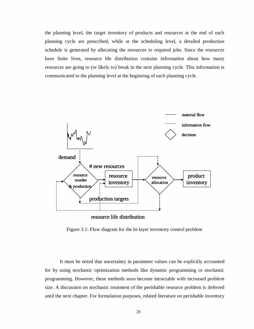
28
the planning level, the target inventory of products and resources at the end of each
planning cycle are prescribed, while at the scheduling level, a detailed production
schedule is generated by allocating the resources to required jobs. Since the resources
have finite lives, resource life distribution contains information about how many
resources are going to (or likely to) break in the next planning cycle. This information is
communicated to the planning level at the beginning of each planning cycle.
resource
reorder
& production
resource
allocation
resource
inventory
product
inventory
demand
resource life distribution
production targets
# new resources
material flow
information flow
decision
resource
reorder
& production
resource
allocation
resource
inventory
product
inventory
demand
resource life distribution
production targets
# new resources
resource
reorder
& production
resource
allocation
resource
inventory
product
inventory
demand
resource life distribution
production targets
# new resources
material flow
information flow
decision
material flow
information flow
decision
Figure 3.1: Flow diagram for the bi-layer inventory control problem
It must be noted that uncertainty in parameter values can be explicitly accounted
for by using stochastic optimization methods like dynamic programming or stochastic
programming. However, these methods soon become intractable with increased problem
size. A discussion on stochastic treatment of the perishable resource problem is deferred
until the next chapter. For formulation purposes, related literature on perishable inventory
29
problem (Haijema et al, 2004), flexible resource allocation (Harrison and Meighem,
1999) and general resource allocation problems (Powell 2007) was reviewed.
Perishable resource problem is distinguished from perishable inventory problem
or a general resource allocation problem (Powell 2007) by at least two complicating
features: (i) the demand for resources is determined by production decisions; therefore
uncertainty is governed by decisions, (ii) there is a strong correlation between the
inventories of products and resources, which need to be controlled simultaneously. For
solution methods, the existing theory on inventory control (Hopp and Spearman, 1996)
and hierarchical treatment of planning and scheduling problem (Miller 2002) was studied.
This chapter is organized as follows. For ease of understanding the formulation
and notation, the stone veneer example is presented in the next section. However, the
concepts and notation are fairly general for systems involving perishable resources. The
solution methods for scheduling and planning levels are discussed in sections 3.3, 3.4 and
3.5. Results and discussion are presented in section 3.6.
3.2. Problem description through stone veneer supply chain
Stone veneer is an artificial stone used in building facades, gardens, etc. for
decorative purposes. It is made by pouring a concrete mixture into molds and letting it
cure. These molds facilitate the production of stones of various shapes and colors. The
molds of a particular shape are painted in different colors to make a variety of nP
different color grades. A mold can only be used once a day, and the facility has limited
capacity (C) in terms of number of molds processed per day. The processing of one mold
is referred to as one „run‟. There are multiple molds in the facility at a given time and
these molds are the resources that are prone to breaking. Therefore, an inventory of molds
needs to be maintained, to satisfy the production needs. In the presence of product
demand uncertainty, stones of various color grades are also kept in store. Finally, the
transition of mold from one color grade to another may lead to further degradation and
eventually cause the mold to break more quickly. The transitions of molds from one color
grade to the other are uni-directional. For example, only transitions from molds of light
30
color grades to dark are allowed. Therefore, the more the fraction of dark molds in the
system, the more inflexible it is in terms of color grade allocation of molds.
In summary, inventory is held at two points in the system (as in Figure 3.1) and
both affect one another. When the molds of a certain color grade fall short of the demand,
the decision-maker may either perform a color grade transition of existing molds at the
expense of flexibility of allocation, or procure new molds at added cost and increased
mold inventory. This trade-off is a unique aspect of this study, coupled with the need to
keep up with product demand. The modeling details on resource age and product demand
are presented in the rest of this section along with the objectives and decisions.
3.2.1 Modeling the resource age
The resource degrades due to general usage and due to transitions from one color
grade to the other. The mold life is modeled as the number of runs it has facilitated. The
loss in transition can be represented as the number of lost runs per transition. This is
captured in the following matrix, where DM stands for degradation matrix and lr for lost
runs. Assuming all color grades of stone cause the same wear and tear on the mold, the
diagonal elements are 1 signifying no transition. A transition from grade 1 to 2 would
cause lr12 >1 number of lost runs.
For modeling purposes, it is assumed that when a new mold enters the system, it has a
finite life ζT associated with it. This implies that the mold would deliver ζT runs before
breaking. ζT can be constant, deterministic or drawn from a distribution leading to
stochastic resource ageing in the latter case.
1....
..............
....1
....1
21
221
112
PP
P
P
nn
n
n
lrlr
lrlr
lrlr
DM
31
3.2.2. Demand modeling
Demands for different types of products are often mutually or temporally
correlated. While the mutual correlation is neglected in this study, the temporal
correlation is addressed by considering the following two cases:
(i) Cyclical demand – In this situation, demand for products follows a repeating trend
as shown in Figure 3.2(a). If one demand scenario represents the set of demands
of nP products at a given time, the scenario repeats every r time periods. E.g., if
we have a single product (nP =1) and r=5, then a cyclical demand pattern can be
represented as in Figure 3.2(b), where the circles show the demand for product
and the arrows show the transition from one scenario to the other over one time
period. In section 3.4.1, this concept is extended to include random transitions
from one scenario to the other. The model is commonly known as a Markov
chain.
(a)
(b)
Figure 3.2: Demand patterns (a) cyclical demand pattern. (b) Cyclical demand pattern
over a 30 unit horizon
32
(ii) Seasonal demand – In this case, the demand for products is low, medium or high
depending on the time of the year. The demand trend is illustrated by an example
with nP =1 in Figure 3.3. Again, the stochastic elements are introduced in section
3.4.
Figure 3.3: A seasonal demand scenario
3.2.3 Resource replenishment lead time and reorder limit
It is assumed that there is a lead time associated with the delivery of new
resources. This implies that new resources are ordered during the current time period,
they will arrive after l time periods, where l is the replenishment lead time. The lead time
is treated as a deterministic parameter in all subsequent analyses. Additionally, there is an
upper limit on reorder quantities of the molds. The restriction is applied to keep the
reorder quantities from fluctuating significantly.
The plant capacity is assumed to be 20 runs per day for all subsequent analysis.
As shown in Figure 3.4, the scheduling time period consists of one day and the
scheduling time horizon h is 10 days. Alternatively, planning time period is consists of 10
days and planning is done over a horizon H of 30 time periods. Due to difference in time
scales, the decision-making is divided between the levels as outlined in section 3.1. At
the planning level, the optimal reorder quantities of the resource and the desired ending
33
inventory of products and resources at the end of each time period are determined. These
values are then communicated to the scheduling level to generate optimal production
schedule while also allocating the resources optimally. The details of formulation are
presented in the next section. To gain an insight into the trade-offs involved, the
deterministic problem is considered first.
0 10 20 40 200 400
run
Scheduling
time period
(1 day)
planning time
period (10 days)
0 10 20 40 200 400
run
Scheduling
time period
(1 day)
planning time
period (10 days)
Figure 3.4: Time scales associated with the planning and scheduling problems considered
in this work.
3.3. Deterministic problem –LP formulation
3.3.1 Deterministic demand and resource life
When the demand for products and number of runs that a resource delivers, have
no associated uncertainty, the problem can be formulated as a linear program (LP) at the
planning level. The planning LP generates optimal production and resource inventory at
the end of each planning period, while satisfying production capacity constraints. Due to
absence of uncertainty, the scheduling level can completely satisfy the inventory targets
prescribed by the solution of planning LP. It is assumed that new orders for resources can
be placed only at the beginning of each planning period and product demand is satisfied
only at the end of planning periods. The detailed formulation is presented below.
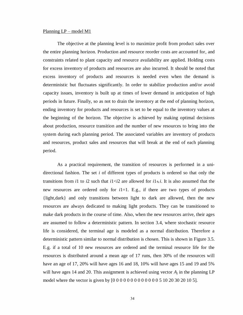
34
Planning LP – model M1
The objective at the planning level is to maximize profit from product sales over
the entire planning horizon. Production and resource reorder costs are accounted for, and
constraints related to plant capacity and resource availability are applied. Holding costs
for excess inventory of products and resources are also incurred. It should be noted that
excess inventory of products and resources is needed even when the demand is
deterministic but fluctuates significantly. In order to stabilize production and/or avoid
capacity issues, inventory is built up at times of lower demand in anticipation of high
periods in future. Finally, so as not to drain the inventory at the end of planning horizon,
ending inventory for products and resources is set to be equal to the inventory values at
the beginning of the horizon. The objective is achieved by making optimal decisions
about production, resource transition and the number of new resources to bring into the
system during each planning period. The associated variables are inventory of products
and resources, product sales and resources that will break at the end of each planning
period.
As a practical requirement, the transition of resources is performed in a uni-
directional fashion. The set i of different types of products is ordered so that only the
transitions from i1 to i2 such that i1<i2 are allowed for i1 i. It is also assumed that the
new resources are ordered only for i1=1. E.g., if there are two types of products
{light,dark} and only transitions between light to dark are allowed, then the new
resources are always dedicated to making light products. They can be transitioned to
make dark products in the course of time. Also, when the new resources arrive, their ages
are assumed to follow a deterministic pattern. In section 3.4, where stochastic resource
life is considered, the terminal age is modeled as a normal distribution. Therefore a
deterministic pattern similar to normal distribution is chosen. This is shown in Figure 3.5.
E.g. if a total of 10 new resources are ordered and the terminal resource life for the
resources is distributed around a mean age of 17 runs, then 30% of the resources will
have an age of 17, 20% will have ages 16 and 18, 10% will have ages 15 and 19 and 5%
will have ages 14 and 20. This assignment is achieved using vector Aj in the planning LP
model where the vector is given by [0 0 0 0 0 0 0 0 0 0 0 0 0 5 10 20 30 20 10 5].
35
% r
eso
urc
esage
+1
+2
+3-3
-2-1
30
20
10
% r
eso
urc
esage
+1
+2
+3-3
-2-1
30
20
10
Figure 3.5: Deterministic initial age distribution of new resources
In the planning LP (model M1), profit is given by the difference of revenue from
product sales and cost of production, resource reorder and holding inventory of products
and resources. Equations M1.1 through M1.4 represent the mass balance of products and
resources. The resources have two associated attributes; the type of product (i) they are
dedicated to making and the number of runs remaining (j). While the mass balance
equations for products are straightforward, those for the resources include the new
arrivals, the degradation of resources due to use (tjijy ,1,3 ) and the transition of resources
from one product type to another (jtiiy ,1,2 ). The degradation term
tjijy ,1,3 represents the
usage of resources during a planning period. Since the planning period has a length h and
a resource can be used only once a day, it cannot be used more than h times. Therefore,
the difference j-j1 must be less than h. It is assumed that no runs are lost in the transition
operation.
In the presence of replenishment lead time l for new resources, information about
previously placed orders that are scheduled to arrive at time t ( 01ijty ) needs to be provided
(equation M1.3). Similarly, the re-order decision variable ijty1 has an associated lag t-l as
shown in equation M1.4.Equation M1.5 represents the fact that product sales cannot
exceed demand and M1.6 through M1.7 place a limit on production in the form of plant
capacity and resource availability respectively. M1.8 assigns ages to newly arrived
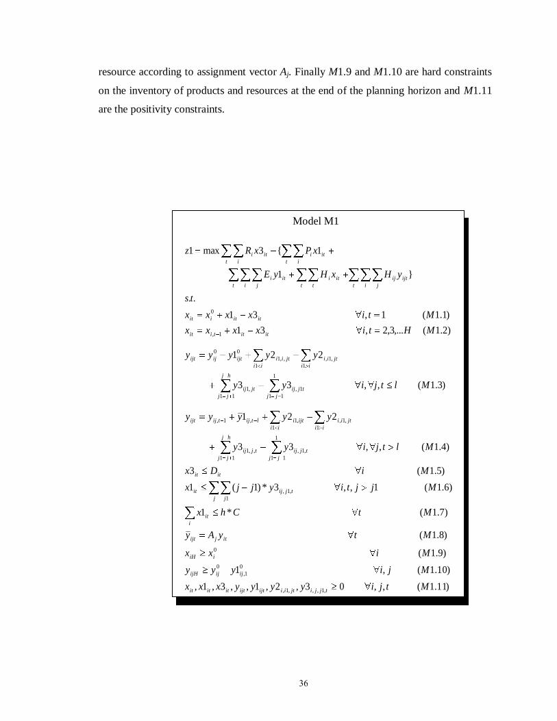
36
resource according to assignment vector Aj. Finally M1.9 and M1.10 are hard constraints
on the inventory of products and resources at the end of the planning horizon and M1.11
are the positivity constraints.
Model M1
)11.1(,,03,2,1,,3,1,
)10.1(,1
)9.1(
)8.1(
)7.1(*1
)6.1(1,,3*)1(1
)5.1(3
)4.1(,,33
221
)3.1(,,33
221
)2.1(,...3,2,31
)1.1(1,31
..
}1
1{3max1
,1,,,1,
0
1,
0
0
,1,
1
1
11
,1,
11
,,1
1
,1,
1
,1,1,
1
11
1,
11
,1
1
,1,
1
,,1
00
1,
0
Mtjiyyyyxxx
Mjiyyy
Mixx
MtyAy
MtChx
Mjjtiyjjx
MiDx
Mltjiyy
yyyyy
Mltjiyy
yyyyy
MHtixxxx
Mtixxxx
ts
yHxHyE
xPxRz
tjjijtiiijtijtititit
ijijijH
iiH
itjijt
i
it
tjij
j j
it
itit
jj
tjij
hj
jj
tjij
ii
jtii
ii
ijtiltijtijijt
jj
tjij
hj
jj
jtij
ii
jtii
ii
jtiiijtijijt
itittiit
ititiit
t i t i
ijt
j
ij
t t
itiit
j
i
t i
iti
t i
iti
37
The deterministic problem is solved for a number of cases with varying parameter
values for product demand and replenishment lead time. The different cases are
summarized in the Table 3.1. Discussion on the results is deferred until section 3.6.
3.4. Dealing with stochastic problems
In most real world situations, parameters like product demand, resource life and
resource replenishment lead time are not deterministic. The concepts and models
developed in the previous section therefore need to be modified. The replenishment lead
time of new resources is considered deterministic in this study since it is possible to
regulate the delivery of the resources by supplier management. Product demand and
resource life are modeled as stochastic parameters as shown below.
3.4.1 Stochastic demand modeling
The stochastic demand in this study is modeled as an extension to the previously
considered demand patterns in section 3.2.2.
(i) Highly fluctuating demand – On similar lines as the cyclical demand pattern, the
demand is modeled as a Markov chain shown in Figure 3.6(a). Each circle
represents a demand scenario, i.e., the set of demands for all products at a given
instant. The arrows emanating from the circle and connecting it to other circles
represent the possible scenarios at the next time period. One of the possible
scenarios is realized at the next time period depending on the probability
associated with the arrow. Starting with a unique demand scenario, the demand
can follow many trajectories with varying probabilities as shown in Figure 3.6(b).
Since it no longer follows a cyclical trend, the pattern is called highly fluctuating
demand.
(ii) Seasonal demand - Instead of considering high, low and medium levels of
demand shown in Figure 3.7(a), the demand is modeled to lie within a band
during each of the three parts of the year. The demand transitions
deterministically from a low to high, and high to medium period, but the
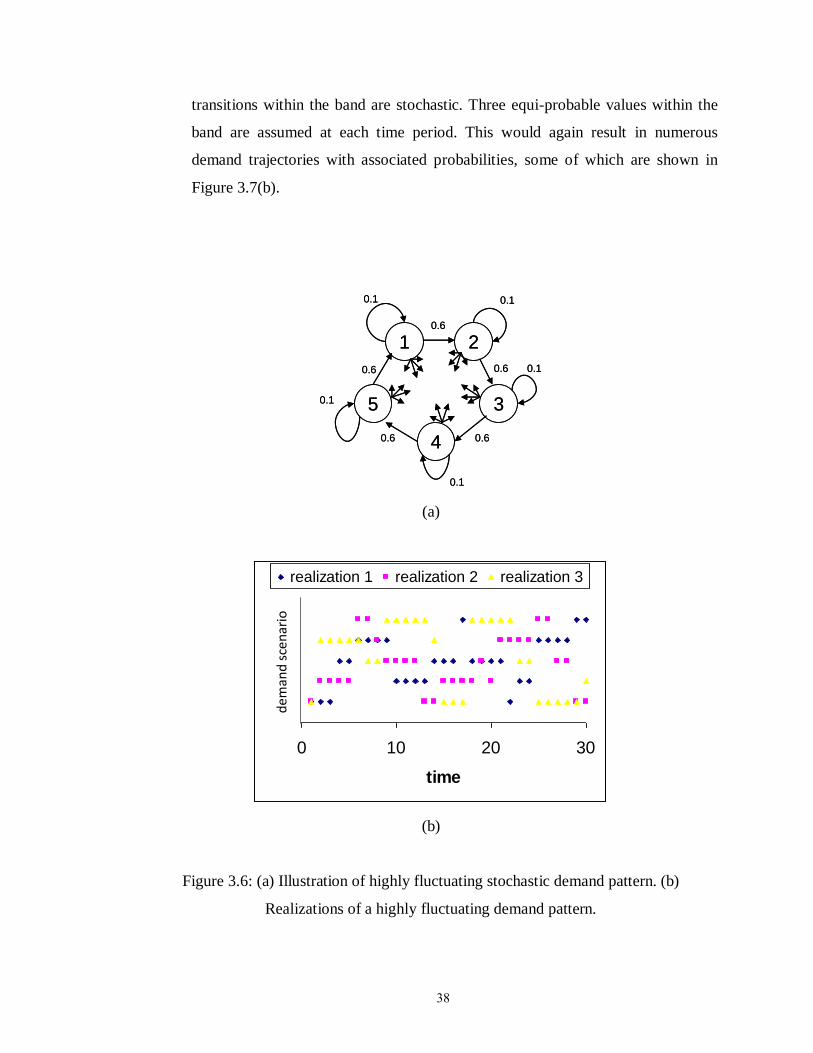
38
transitions within the band are stochastic. Three equi-probable values within the
band are assumed at each time period. This would again result in numerous
demand trajectories with associated probabilities, some of which are shown in
Figure 3.7(b).
1 2
35
4
0.1
0.6
0.6
0.6
0.6
0.6
0.1
0.1
0.1
0.1
1 2
35
4
0.1
0.6
0.6
0.6
0.6
0.6
0.1
0.1
0.1
0.1
(a)
0 10 20 30
time
dem
an
d s
cen
ari
o
realization 1 realization 2 realization 3
0 10 20 30
time
dem
an
d s
cen
ari
o
realization 1 realization 2 realization 3
(b)
Figure 3.6: (a) Illustration of highly fluctuating stochastic demand pattern. (b)
Realizations of a highly fluctuating demand pattern.
dem
and
sce
nar
io
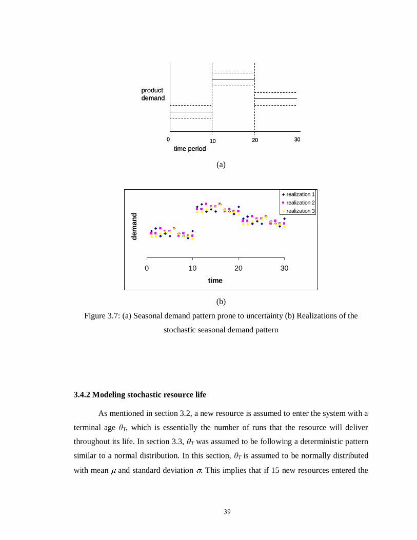
39
0 10 20 30
product
demand
time period
0 10 20 30
product
demand
time period
(a)
0 10 20 30
time
dem
an
d
realization 1
realization 2
realization 3
(b)
Figure 3.7: (a) Seasonal demand pattern prone to uncertainty (b) Realizations of the
stochastic seasonal demand pattern
3.4.2 Modeling stochastic resource life
As mentioned in section 3.2, a new resource is assumed to enter the system with a
terminal age ζT, which is essentially the number of runs that the resource will deliver
throughout its life. In section 3.3, ζT was assumed to be following a deterministic pattern
similar to a normal distribution. In this section, ζT is assumed to be normally distributed
with mean and standard deviation . This implies that if 15 new resources entered the
40
system at time t and ζT (17,2) then a possible realization of resource life distribution is
[0 0 0 0 0 0 0 0 0 0 0 0 0 0 1 3 4 4 0 2 1] and several such realizations are possible.
3.4.3 Solving the stochastic problem
In usual practice, the planning problem is solved for projected future demand for
products. The optimal ending inventory for products and resources is then generated
using the LP described in previous section. Therefore, the desired inventory at the end of
each 10 day period is known. During these 10 days, the scheduling level generates a
detailed production schedule and resource allocation schedule to meet the ending
inventory requirement at the end of the 10 day period. However, when resource durability
and product demand have associated uncertainty, the ending inventory values of products
and the resource life profile are not the same as predicted by the planning LP. The actual
inventory values and resource life distribution need to be communicated to the planning
LP at the end of each planning period. This is achieved by solving the LP in a rolling
horizon fashion as shown in Figure 3.8. At the beginning of the horizon, the LP is solved
for 30 time periods and the ending inventory targets for products and resources are
generated. The decisions about resource reorder, production etc. are implemented at the
beginning of the horizon. At the end of first time period, the age distribution of the new
resources and the actual product demand become available. The horizon is shifted by one
time period and the LP is solved again for next 30 time periods starting with the actual
values of product inventory and resource life distribution.
Moreover, the ending inventory targets prescribed by the planning level may not
be feasible at the scheduling level. E.g., if the demand for products at the end of last
planning period was substantially higher than the projected value, the system is left with
lower inventories at the beginning of the current period. Production capacity and resource
limits may not allow enough production for the scheduling level to match the ending
inventory target. Alternatively, if the resource lives are realized to be lower than
expected, then the resource availability may not be enough to produce goods up to the
prescribed inventory targets. Consequently, an optimization problem at the scheduling
41
level needs to be solved taking into account the actual starting inventory and actual
number of runs available from the resources at the beginning of each planning period.
The time horizon h for the scheduling period is 10 days (equal to one planning period)
and one scheduling time period is one day. The difference in time scales of planning and
scheduling are shown in Figure 3.4 and the scheduling LP is shown by model M2.
The scheduling LP has similar mass balance equations, capacity constraints,
resource allocation and transition variables as contained in the planning LP. The
production, inventory, transition and allocation variables in this case are designated with
a tilda (~) sign to differentiate from those at the planning level. The important differences
from the planning LP being:
(i) Resource reorder and product sales are not a part of the decision-making
(ii) Since revenue is not being generated at this level, the objective is to minimize
cost of production while meeting the ending inventory targets at the end of the
scheduling horizon (10 days) as prescribed by the planning LP. The latter is
modeled as penalty variables penalty1i, penalty2i as shown in the model. If the
system ends up with less inventory of product i, i=1,2,..nP and less number of
remaining runs to make product i, i=1,2.. nP (equations M2.7 and M2.8), a cost
proportional to the difference is added in the objective function. Weights w1 and
w2 are reasonably chosen parameters.
(iii) As per the assumptions stated in section 3.2, the resource delivers one run in one
scheduling period as shown using allocation variables y3ijt in equations M2.3 and
M2.4.
(iv) The total production in one scheduling period cannot exceed the system capacity
of C runs/day as shown by capacity constraint M2.6.
(v) The ending inventory of products ( ihx~ ) and number of runs remaining from the
resources ( ijhyj ~* ) are targeted to be more than or equal to those prescribed by
the planning LP ( 1ix , 1* ijyj ). This is accomplished by constraints M2.7 and M2.8
as described in point (ii).
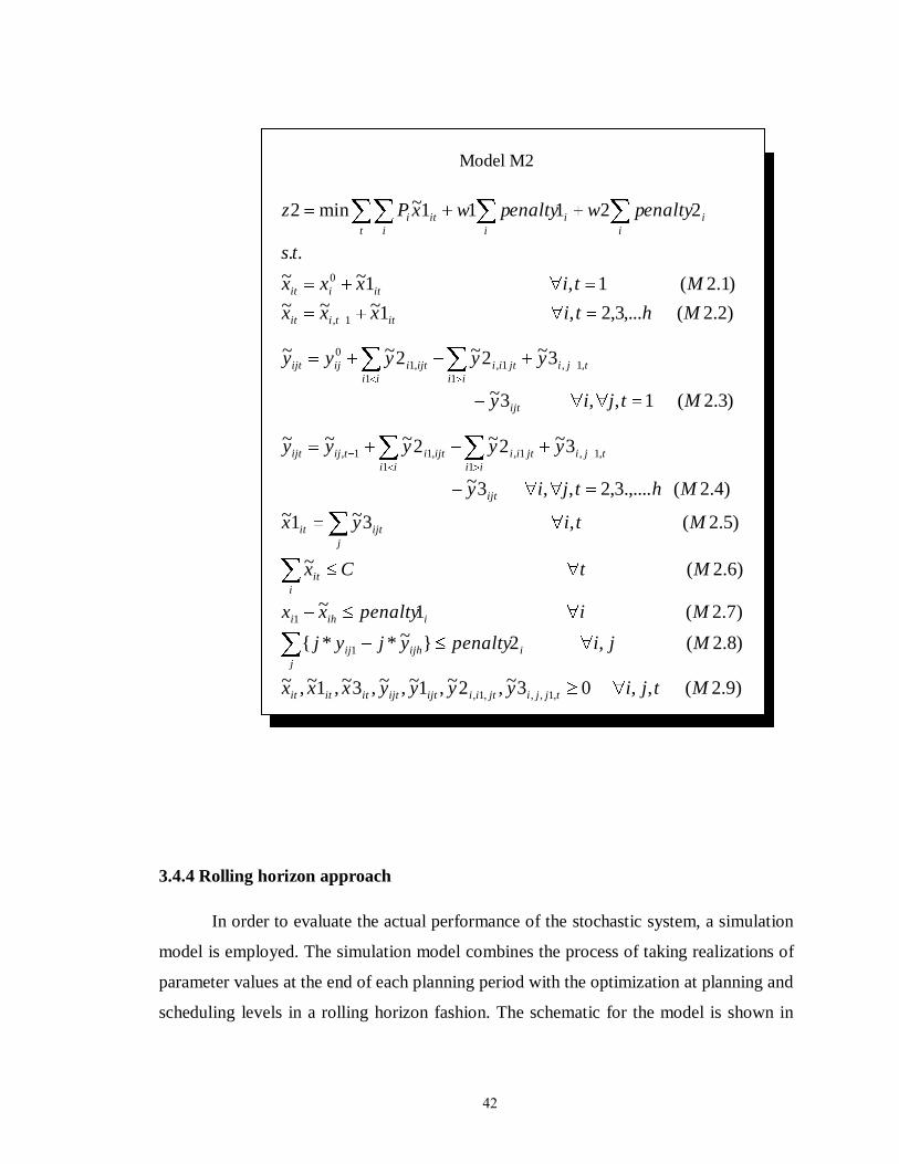
42
Model M2
)9.2(,,03~,2~,1~,~,3~,1~,~
)8.2(,2}~**{
)7.2(1~
)6.2(~
)5.2(,3~1~
)4.2(.,....3,2,,3~
3~2~2~~~
)3.2(1,,3~
3~2~2~~
)2.2(,...3,2,1~~~)1.2(1,1~~
..
22111~min2
,1,,,1,
1
1
,1,
1
1,
1
,11,
,1,
1
1,
1
,1
0
1,
0
Mtjiyyyyxxx
Mjipenaltyyjyj
Mipenaltyxx
MtCx
Mtiyx
Mhtjiy
yyyyy
Mtjiy
yyyyy
Mhtixxx
Mtixxx
ts
enaltypwenaltypwxPz
tjjijtiiijtijtititit
iijhij
j
iihi
i
it
j
ijtit
ijt
tji
ii
jtii
ii
ijtitijijt
ijt
tji
ii
jtii
ii
ijtiijijt
ittiit
itiit
i
i
i
it i
iti
3.4.4 Rolling horizon approach
In order to evaluate the actual performance of the stochastic system, a simulation
model is employed. The simulation model combines the process of taking realizations of
parameter values at the end of each planning period with the optimization at planning and
scheduling levels in a rolling horizon fashion. The schematic for the model is shown in
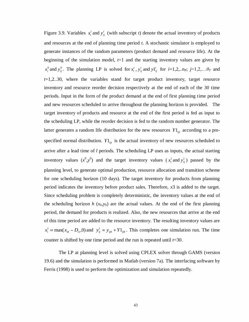
43
Figure 3.9. Variables t
ix and t
ijy (with subscript t) denote the actual inventory of products
and resources at the end of planning time period t. A stochastic simulator is employed to
generate instances of the random parameters (product demand and resource life). At the
beginning of the simulation model, t=1 and the starting inventory values are given by
0
ix and 0
ijy . The planning LP is solved for t
ix , t
ijy and t
ijy1 for i=1,2,..nP; j=1,2,…ζT and
t=1,2..30, where the variables stand for target product inventory, target resource
inventory and resource reorder decision respectively at the end of each of the 30 time
periods. Input in the form of the product demand at the end of first planning time period
and new resources scheduled to arrive throughout the planning horizon is provided. The
target inventory of products and resource at the end of the first period is fed as input to
the scheduling LP, while the reorder decision is fed to the random number generator. The
latter generates a random life distribution for the new resources ijtY1 according to a pre-
specified normal distribution. ijtY1 is the actual inventory of new resources scheduled to
arrive after a lead time of l periods. The scheduling LP uses as inputs, the actual starting
inventory values (x0,y
0) and the target inventory values ( 1
ix and 1
ijy ) passed by the
planning level, to generate optimal production, resource allocation and transition scheme
for one scheduling horizon (10 days). The target inventory for products from planning
period indicates the inventory before product sales. Therefore, x3 is added to the target.
Since scheduling problem is completely deterministic, the inventory values at the end of
the scheduling horizon h (xh,yh) are the actual values. At the end of the first planning
period, the demand for products is realized. Also, the new resources that arrive at the end
of this time period are added to the resource inventory. The resulting inventory values are
)0,max( 1
1
iihi Dxx and ijhijhij Yyy 11. This completes one simulation run. The time
counter is shifted by one time period and the run is repeated until t=30.
The LP at planning level is solved using CPLEX solver through GAMS (version
19.6) and the simulation is performed in Matlab (version 7a). The interfacing software by
Ferris (1998) is used to perform the optimization and simulation repeatedly.
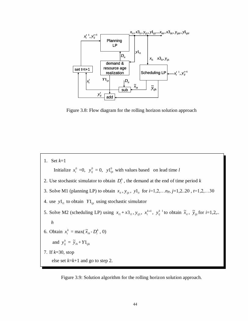
44
Planning
LP
Scheduling LP
1t
ijy,1t
ixijHijHiHiHijijii yyxxyyxx 1,,3,....1,,3, 1111
111 ,3 ijii yxx
11iy
ihx~ijhy~
demand &
resource age
realization
sub
add
itD
itD
1t
ijy,1t
ix
t
ijy
t
ix ijtY1
set t=t+1
Planning
LP
Scheduling LP
1t
ijy,1t
ixijHijHiHiHijijii yyxxyyxx 1,,3,....1,,3, 1111
111 ,3 ijii yxx
11iy
ihx~ijhy~
demand &
resource age
realization
sub
add
itD
itD
1t
ijy,1t
ix
t
ijy
t
ix ijtY1
set t=t+1
Figure 3.8: Flow diagram for the rolling horizon solution approach
1. Set k=1
Initialize 0
ix =0, 0
ijy = 0, 01ijty with values based on lead time l
2. Use stochastic simulator to obtain k
iD , the demand at the end of time period k
3. Solve M1 (planning LP) to obtain itx , ijty , ity1 for i=1,2,…nP, j=1,2..20 , t=1,2,…30
4. use 11iy to obtain ijtY1 using stochastic simulator
5. Solve M2 (scheduling LP) using 1ix + 13ix , 1ijy , 1k
ix , 1k
ijy to obtain itx~ , ijty~ for i=1,2,..
h
6. Obtain k
ix = max( ihx~ - k
iD , 0)
and k
ijy = ihy~ + ijkY1
7. If k=30, stop
else set k=k+1 and go to step 2.
Figure 3.9: Solution algorithm for the rolling horizon solution approach.

45
An important thing to note is that when the deterministic demand forecast for the
next H time periods is fed into the planning LP, a buffer needs to be maintained so that
the fluctuations in future demand are accounted for. A conservative heuristic is employed
to this end, by inclusion of a pre-determined buffer stock or safety stock ss, where ss is
treated as a parameter to be optimized. E.g. 10% extra is added to the forecast. Any
excess is automatically corrected at the next time period.
The rolling horizon approach is conventionally applied to planning and
scheduling problems for production planning independent of resource planning which is
done separately. This is shown in the next section.
3.5. The decoupled problem
In order to gauge the effectiveness of solving the coupled problem, the decoupled
problem is also solved. This implies that the resource reorder and production planning
decisions are considered independent of each other (conventional practice).
3.5.1 Resource reorder
Resource procurement, when treated independent of production planning, is a
standard inventory control problem with stochastic demand. In such a scenario, a policy
of the form (s,S) is proven optimal for given demand distributions and provides a good
approximation for the others. The parameter s is the reorder point and S is the reorder
quantity. The optimal plan is to place an order whenever the stock is equal to or falls
below s to bring the inventory to level S and do nothing otherwise. Since there is no fixed
cost associated with placing a new order in the system considered, s is very high. The
policy in this case is to always bring the stock of resources up to level S, where S is the
only parameter to be optimized. Taking note of the flexibility of the resources and the
fact that the resources deliver multiple runs, different quantities may be considered as
stock in this case. E.g.,
(i) Total number of resources at any time
(ii) Separate parameters for different types of resources (Si for i=1,2,…nP)
(iii) Total number of runs available from all the resources.
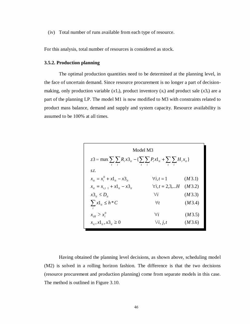
46
(iv) Total number of runs available from each type of resource.
For this analysis, total number of resources is considered as stock.
3.5.2. Production planning
The optimal production quantities need to be determined at the planning level, in
the face of uncertain demand. Since resource procurement is no longer a part of decision-
making, only production variable (x1i), product inventory (xi) and product sale (x3i) are a
part of the planning LP. The model M1 is now modified to M3 with constraints related to
product mass balance, demand and supply and system capacity. Resource availability is
assumed to be 100% at all times.
Model M3
)6.3(,,03,1,
)5.3(
)4.3(*1
)3.3(3
)2.3(,...3,2,31
)1.3(1,31
..
}1{3max3
0
1,
0
Mtjixxx
Mixx
MtChx
MiDx
MHtixxxx
Mtixxxx
ts
xHxPxRz
ititit
iiH
i
it
itit
itittiit
ititiit
t i
iti
t i
iti
t i
iti
Having obtained the planning level decisions, as shown above, scheduling model
(M2) is solved in a rolling horizon fashion. The difference is that the two decisions
(resource procurement and production planning) come from separate models in this case.
The method is outlined in Figure 3.10.
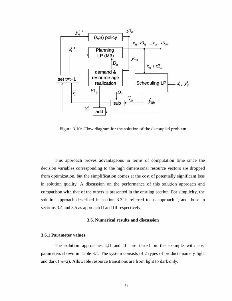
47
Planning
LP (M3)
Scheduling LP
1t
ijy
,1t
ix
iHiHii xxxx 3,,....3, 11
11 3ii xx
11iy
ihx~ijhy~
demand &
resource age
realization
sub
add
itD
itD
t
ijy,t
ix
t
ijy
t
ix ijtY1
set t=t+1
(s,S) policy
11iy
Planning
LP (M3)
Scheduling LP
1t
ijy
,1t
ix
iHiHii xxxx 3,,....3, 11
11 3ii xx
11iy
ihx~ijhy~
demand &
resource age
realization
sub
add
itD
itD
t
ijy,t
ix
t
ijy
t
ix ijtY1
set t=t+1
(s,S) policy
11iy
Figure 3.10: Flow diagram for the solution of the decoupled problem
This approach proves advantageous in terms of computation time since the
decision variables corresponding to the high dimensional resource vectors are dropped
from optimization, but the simplification comes at the cost of potentially significant loss
in solution quality. A discussion on the performance of this solution approach and
comparison with that of the others is presented in the ensuing section. For simplicity, the
solution approach described in section 3.3 is referred to as approach I, and those in
sections 3.4 and 3.5 as approach II and III respectively.
3.6. Numerical results and discussion
3.6.1 Parameter values
The solution approaches I,II and III are tested on the example with cost
parameters shown in Table 3.1. The system consists of 2 types of products namely light
and dark (nP=2). Allowable resource transitions are from light to dark only.
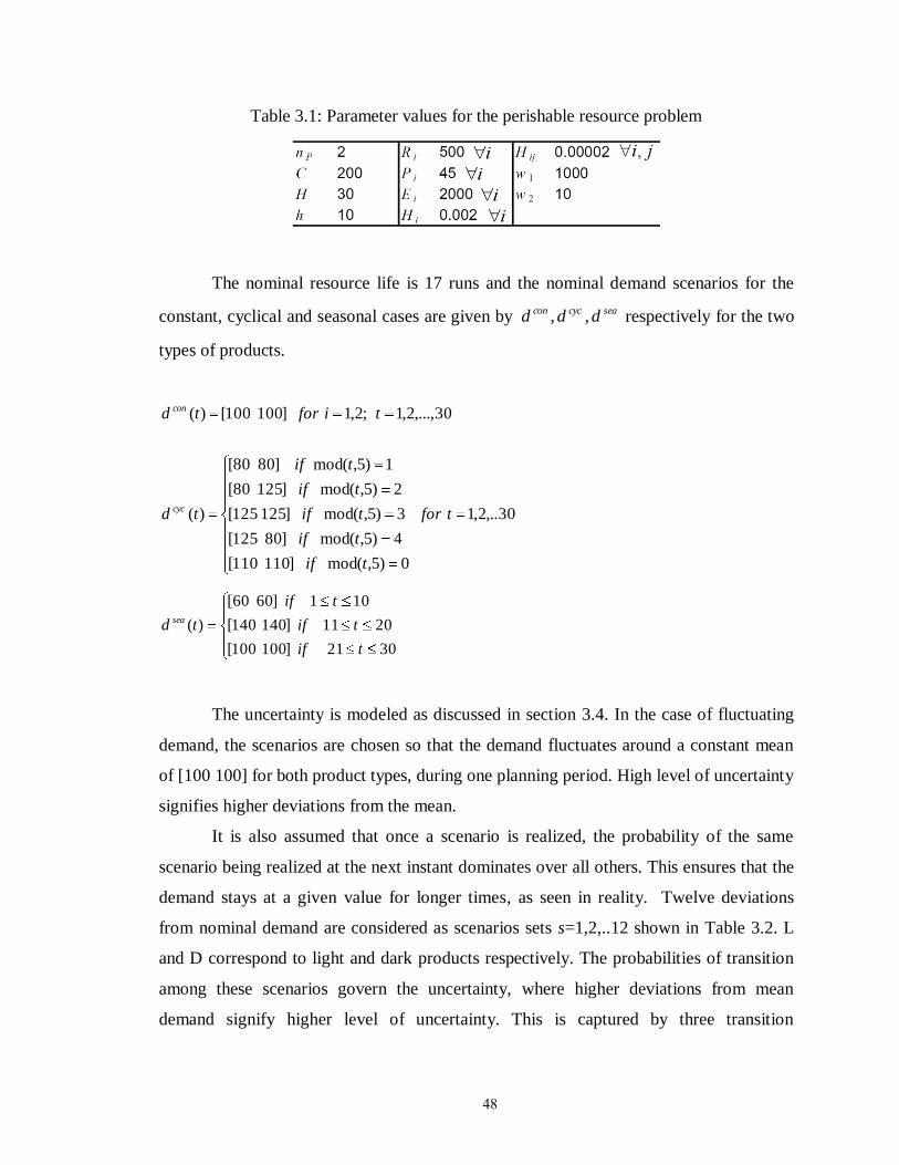
48
Table 3.1: Parameter values for the perishable resource problem
The nominal resource life is 17 runs and the nominal demand scenarios for the
constant, cyclical and seasonal cases are given by seacyccon ddd ,, respectively for the two
types of products.
30,..2,1
0)5,mod(]110110[
4)5,mod(]80125[
3)5,mod(]125125[
2)5,mod(]12580[
1)5,mod(]8080[
)(
30,...,2,1;2,1]100100[)(
tfor
tif
tif
tif
tif
tif
td
tifortd
cyc
con
3021]100100[
2011]140140[
101]6060[
)(
tif
tif
tif
td sea
The uncertainty is modeled as discussed in section 3.4. In the case of fluctuating
demand, the scenarios are chosen so that the demand fluctuates around a constant mean
of [100 100] for both product types, during one planning period. High level of uncertainty
signifies higher deviations from the mean.
It is also assumed that once a scenario is realized, the probability of the same
scenario being realized at the next instant dominates over all others. This ensures that the
demand stays at a given value for longer times, as seen in reality. Twelve deviations
from nominal demand are considered as scenarios sets s=1,2,..12 shown in Table 3.2. L
and D correspond to light and dark products respectively. The probabilities of transition
among these scenarios govern the uncertainty, where higher deviations from mean
demand signify higher level of uncertainty. This is captured by three transition
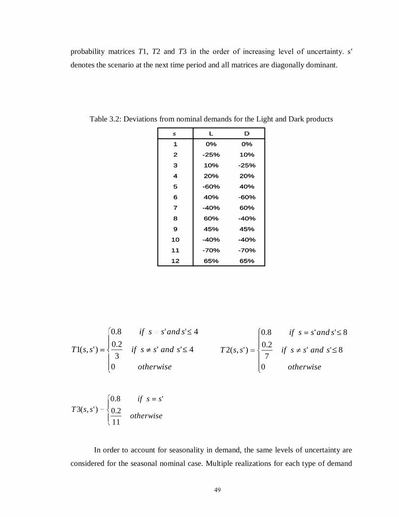
49
probability matrices T1, T2 and T3 in the order of increasing level of uncertainty. s′
denotes the scenario at the next time period and all matrices are diagonally dominant.
Table 3.2: Deviations from nominal demands for the Light and Dark products
65%65%12
-70%-70%11
-40%-40%10
45%45%9
-40%60%8
60%-40%7
-60%40%6
40%-60%5
20%20%4
-25%10%3
10%-25%2
0%0%1
DLs
65%65%12
-70%-70%11
-40%-40%10
45%45%9
-40%60%8
60%-40%7
-60%40%6
40%-60%5
20%20%4
-25%10%3
10%-25%2
0%0%1
DLs
otherwise
sandssif
sandssif
ssT
0
4''3
2.0
4''8.0
)',(1
otherwise
sandssif
sandssif
ssT
0
8''7
2.0
8''8.0
)',(2
otherwise
ssif
ssT
11
2.0
'8.0
)',(3
In order to account for seasonality in demand, the same levels of uncertainty are
considered for the seasonal nominal case. Multiple realizations for each type of demand
50
(constant and seasonal mean) and each level of uncertainty (low, medium and high) are
considered to obtain average performance. (It must be noted that there are 1230
possible
realizations, making the probability of an individual realization miniscule. Therefore
obtaining a true average is very difficult). The realizations are drawn at random and are
fixed for the different solution approaches. The comparison is mostly scenario based.
Resource life is modeled as a normal distribution with mean of 17 runs. Low, medium
and high levels of uncertainty correspond to standard deviations of 0.5, 1 and 2
respectively.
3.6.2 Features
The models and solution approaches described throughout this article are tested
along the features listed in Table 3.3, where lead time is the delay associated with
resource order arrival, safety stock is the buffer added to the demand forecast. Two types
of demands and three levels of uncertainty are considered as discussed. Various revenue
and cost heads are reported in Table 3.4 for some of the cases. Average resource
utilization defined as the ratio of total number of resources used and the total number of
resources in the system is also reported along with the total missed demand to highlight
the instances of lost opportunity. The effects of aforementioned features are examined
after some general observations outlined below:
(i) Product sales contribute highest to the overall profit. Therefore, satisfying product
demand is the chief driver for all solution approaches. The higher the missed
demand, the worse is the performance.
(ii) The optimal issuing policy is to use the oldest resources and optimal transition
policy is from oldest light resource to dark.
(iii) Different demand trajectories sum to different values of overall demand.
Therefore, profit is scaled by the overall demand as the objective value in all
analyses.
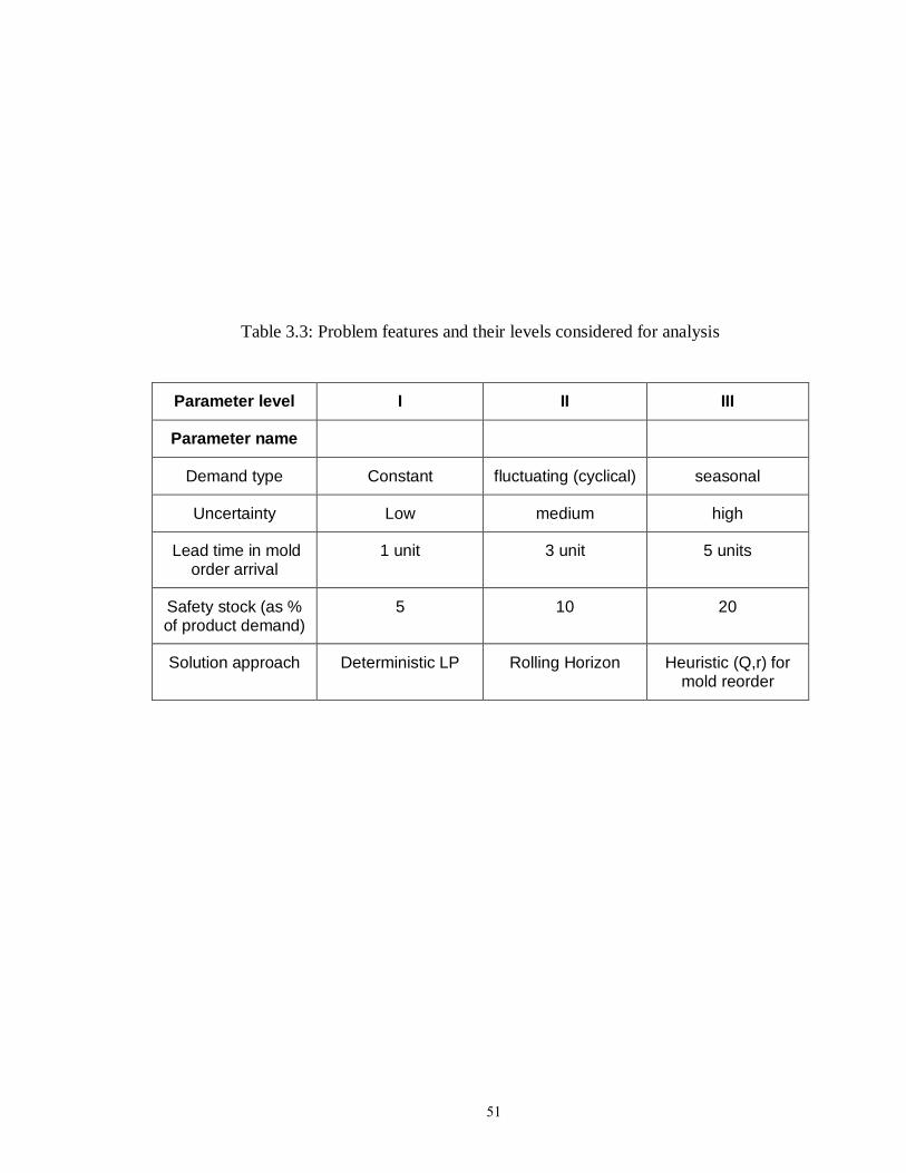
51
Table 3.3: Problem features and their levels considered for analysis
Parameter level I II III
Parameter name
Demand type Constant fluctuating (cyclical) seasonal
Uncertainty Low medium high
Lead time in mold order arrival
1 unit 3 unit 5 units
Safety stock (as % of product demand)
5 10 20
Solution approach Deterministic LP Rolling Horizon Heuristic (Q,r) for mold reorder
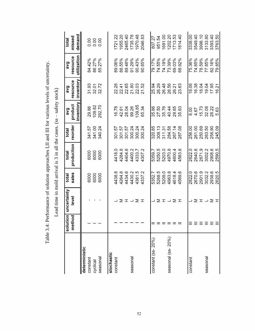
52
Tab
le 3
.4:
Per
form
ance
of
solu
tion a
ppro
aches
I,I
I an
d I
II f
or
var
ious
level
s of
unce
rtai
nty
.
Lea
d t
ime
in m
old
arr
ival
is
3 i
n a
ll t
he
case
s. (
ss –
saf
ety s
tock
)
53
The effects of different features are now discussed:
A. Effect of time varying demand
To analyze the effect of time varying demand, the deterministic demand and
resource life scenarios are studied. For three types of demand (constant, cyclical and
seasonal), substantial difference lies in the values of average product inventories as seen
in Figure 3.11(a). This is because when demand is uneven, inventory is built up
beforehand. Nominal seasonal demand has higher deviations from the constant trajectory
and therefore has higher average inventory of products. As a result, the production is
leveled, as seen by the similar average resource inventories. The other revenue and cost
heads are the same because although the demand deviates, it is known completely to the
decision-maker.
B. Effect of uncertainty
In most cases, higher uncertainty results in lower performance in terms of profit
per unit of demand for both approaches (I and II) as shown in Figure 3.11(b). This is also
reflected in increasing values of missed demand. It is seen that although the resource
reorder quantities are similar to the deterministic solution (imposed to be equal for
approach I), the average resource inventories in both cases are lower. This signifies more
resource breakage due to uncertainty in resource lives.
C. Lead time
Increase in lead time results in worse performance by both solution approaches (I
and II) as seen in Figure 3.11(c). The result is expected because the further out into the
future we look, the more uncertain demand gets.
D. Safety stock
Four values of safety stock or demand buffer are considered for approach II. In
both demand profiles, 20% safety stock is the best heuristic (Figure 3.11(d)). As safety
stock is increased further, the system keeps more inventory of products than required, and
54
one product cannibalizes the other in terms of its share of resources and production
capacity.
E. Solution approaches
A comparison of the performance of the three approaches (I,II and III) is shown in
Figure 3.11 (e) for the two types of demand (constant nominal demand and seasonal
nominal demand). The decoupled problem (approach III), is solved for several values of
S (30,35,40,45,50), where S is the maximum stock level. The best value for S is found to
be 35 and the results are reported for this value only. It is seen that decoupled problem in
all cases performs significantly worse than the LP without update and the rolling horizon
approach. As much as 50% demand is missed in certain cases when using approach III.
This confirms that treating resource procurement and production planning decisions
together is imperative. The decoupled problem would perform particularly badly when
the total resource usage varies significantly from one period to the other. The latter is
likely in most practical situations when either the product demand deviates significantly
from the mean or resource allocation causes varying number of resources to perish.
The rolling horizon approach performs 12-20% better than LP without update.
However, it is seen that the performance gap reduces with increasing level of uncertainty
which highlights the fact that rolling horizon cannot handle very high deviations from the
expected values of uncertainty. This necessitates the use of solution methods that can
explicitly account for uncertainty during optimization.
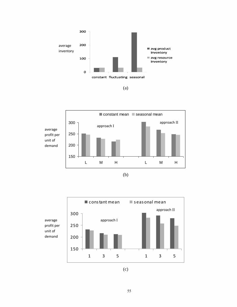
55
(a)
150
200
250
300
L M H L M H
constant mean seasonal mean
(b)
150
200
250
300
1 3 5 1 3 5
cons tant mean s eas onal mean
(c)
average
inventory
average
profit per
unit of
demand
approach I approach II
approach I
approach II
average
profit per
unit of
demand
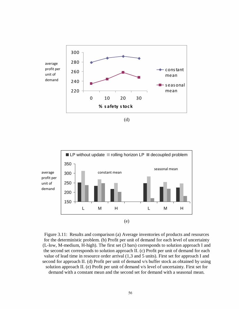
56
220
240
260
280
300
0 10 20 30
% s afety s toc k
cons tantmean
s eas onalmean
(d)
150
200
250
300
350
L M H L M H
LP without update rolling horizon LP decoupled problem
(e)
Figure 3.11: Results and comparison (a) Average inventories of products and resources
for the deterministic problem. (b) Profit per unit of demand for each level of uncertainty
(L-low, M-medium, H-high). The first set (3 bars) corresponds to solution approach I and
the second set corresponds to solution approach II. (c) Profit per unit of demand for each
value of lead time in resource order arrival (1,3 and 5 units). First set for approach I and
second for approach II. (d) Profit per unit of demand v/s buffer stock as obtained by using
solution approach II. (e) Profit per unit of demand v/s level of uncertainty. First set for
demand with a constant mean and the second set for demand with a seasonal mean.
average
profit per
unit of
demand
average
profit per
unit of
demand
constant mean seasonal mean
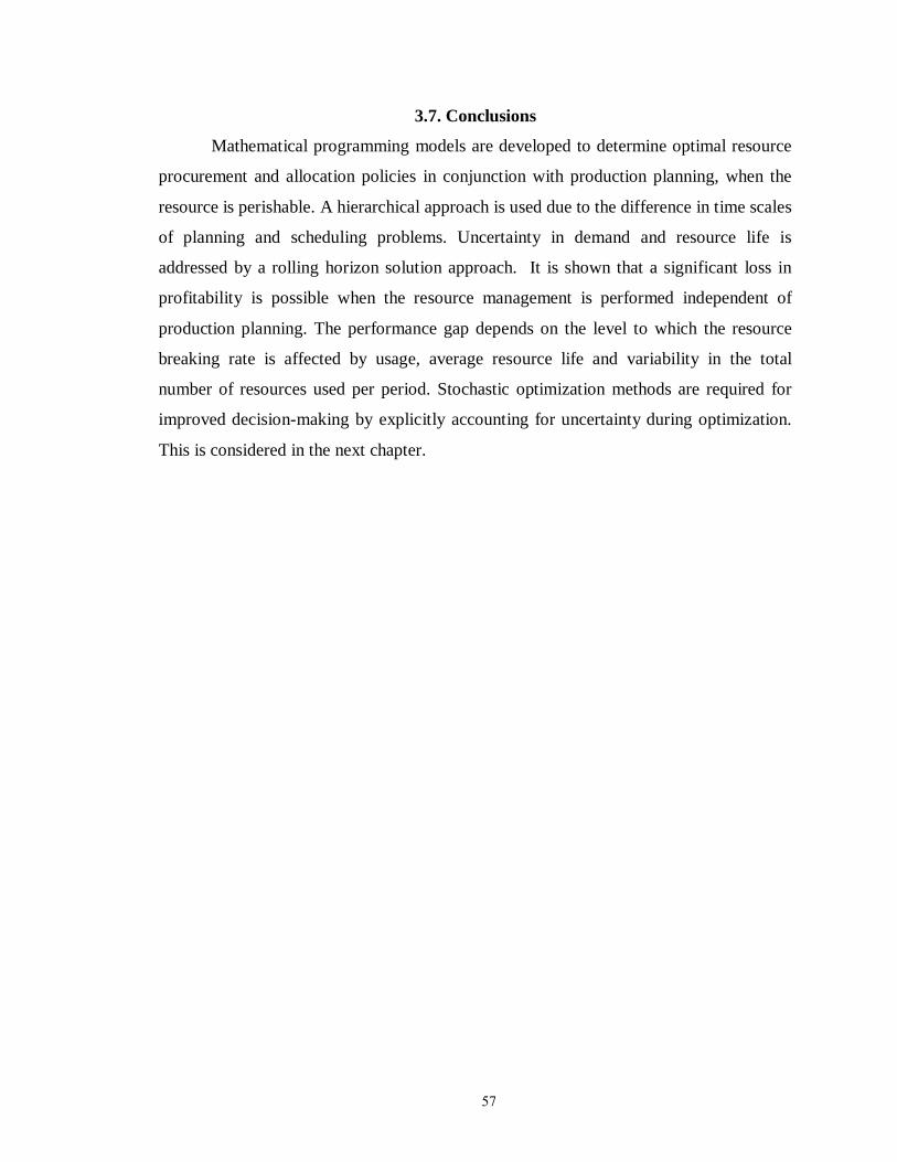
57
3.7. Conclusions
Mathematical programming models are developed to determine optimal resource
procurement and allocation policies in conjunction with production planning, when the
resource is perishable. A hierarchical approach is used due to the difference in time scales
of planning and scheduling problems. Uncertainty in demand and resource life is
addressed by a rolling horizon solution approach. It is shown that a significant loss in
profitability is possible when the resource management is performed independent of
production planning. The performance gap depends on the level to which the resource
breaking rate is affected by usage, average resource life and variability in the total
number of resources used per period. Stochastic optimization methods are required for
improved decision-making by explicitly accounting for uncertainty during optimization.
This is considered in the next chapter.
58
CHAPTER 4
AN APPROXIMATE DYNAMIC PROGRAMMING APPROACH
TO SOLVING PLANNING AND SCHEDULING PROBLEMS WITH
PERISHABLE RESOURCES
In the previous chapter, mathematical programs were developed for planning and
scheduling with perishable resources. In the presence of uncertainty in product demand
and resource life, the hierarchical framework was implemented in a rolling horizon
fashion. This enabled the presence of a feedback loop to update the knowledge of system
attributes at each time step. While solving the LP in a rolling horizon fashion, the most
probable realization of uncertainty is considered. Therefore, the performance of the
rolling horizon approach is determined greatly by the form of uncertainty. In general, the
rolling horizon approach is well suited for problems where there is little likelihood of
sudden and radical changes in the uncertain parameter. This is because the rolling horizon
approach provides a reactive mechanism, which takes corrective action once the
deviation from the most probable realization (or trajectory) is registered. In other words,
the rolling horizon approach only has a myopic view of the uncertainty. For most
applications however, the myopic view of the uncertainty does not suffice and proactive
mechanism is desired. For such problems, exclusively accounting for the uncertainty
during optimization is imperative. A particular example of problems requiring fore-sight
with respect to parametric uncertainty is, when the problem attributes are changed
permanently and drastically by decisions. In an inventory control problem, this situat ion
may arise when the product demand inflates or falls rapidly, and the firm‟s performance
during these scenarios determines its long run market share. The same is true for pricing
problems. This aspect is explained by means of an illustration in 4.1. The perishable
resource problem is then reconsidered and the planning problem is formulated as a
Markov Decision Process (MDP) in section 4.2.1. MDP is an elegant framework to solve
stochastic decision problems. Owing to the large state and action spaces, an approximate
dynamic programming (ADP) algorithm is employed and discussed in detail in section
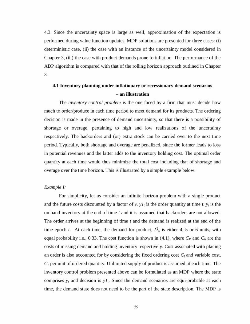
59
4.3. Since the uncertainty space is large as well, approximation of the expectation is
performed during value function updates. MDP solutions are presented for three cases: (i)
deterministic case, (ii) the case with an instance of the uncertainty model considered in
Chapter 3, (iii) the case with product demands prone to inflation. The performance of the
ADP algorithm is compared with that of the rolling horizon approach outlined in Chapter
3.
4.1 Inventory planning under inflationary or recessionary demand scenarios
– an illustration
The inventory control problem is the one faced by a firm that must decide how
much to order/produce in each time period to meet demand for its products. The ordering
decision is made in the presence of demand uncertainty, so that there is a possibility of
shortage or overage, pertaining to high and low realizations of the uncertainty
respectively. The backorders and (or) extra stock can be carried over to the next time
period. Typically, both shortage and overage are penalized, since the former leads to loss
in potential revenues and the latter adds to the inventory holding cost. The optimal order
quantity at each time would thus minimize the total cost including that of shortage and
overage over the time horizon. This is illustrated by a simple example below:
Example I:
For simplicity, let us consider an infinite horizon problem with a single product
and the future costs discounted by a factor of γ. y1t is the order quantity at time t. yt is the
on hand inventory at the end of time t and it is assumed that backorders are not allowed.
The order arrives at the beginning of time t and the demand is realized at the end of the
time epoch t. At each time, the demand for product, t, is either 4, 5 or 6 units, with
equal probability i.e., 0.33. The cost function is shown in (4.1), where CP and Ch are the
costs of missing demand and holding inventory respectively. Cost associated with placing
an order is also accounted for by considering the fixed ordering cost Cf and variable cost,
Cv per unit of ordered quantity. Unlimited supply of product is assumed at each time. The
inventory control problem presented above can be formulated as an MDP where the state
comprises yt and decision is y1t. Since the demand scenarios are equi-probable at each
time, the demand state does not need to be the part of the state description. The MDP is
60
solved using value iteration (described in section 2.4 of Chapter 2) and the optimal policy
πI is as shown in (4.2) for CP =1 Cf= 0.3 and Cv=0.2, and Ch =0.1. It is a well known
result (Hopp and Spearman, 1996), that the optimal policy is of the parametric form (s,S)
when the uncertainty has an underlying Markov chain. The parametric form of the policy
translates into placing an order whenever the inventory falls below s to bring it up to S.
tvtf
tttPttthtt
yCyC
yyDCDyyCDyE
1)01(
}0,1~
max{}0,~
1max{)~
,( 111 (4.1)
otherwise5
4if01
t
t
ty
yy (4.2)
A variation in the demand model is considered next. Example II is used to
illustrate the dependence of future demands on firm‟s performance during a temporary
surge in demand. The example is motivated by the fact that if the firm continually misses
demand, the goodwill of the firm would be affected. This might result in permanent loss
of some customers or loss of market share. Consequently, the firm may see reduced
demand when the inflation in demand subsides.
Example II:
Figure 4.1(a) shows a demand model where the product demand can be in one of
the three states ζ {1,2,4}. The first state, i.e., ζ=1 is similar to one in example I, where
demand can be 4,5 or 6 units with equal probability (designated as 5±1). This is referred
to as the nominal demand state. At each time, with finite probability, demand may
transition to an inflationary state designated by circle 2. State 2, i.e., ζ=2, represents the
case of increased demands for goods due to boom in the economy, industry growth or
other socio-economic or technology related factor. Once in state 2, the system may
transition back to nominal demand state, i.e., ζ=1 with finite probability at each time. The
demand in state ζ=2 is 10±1, where all three values are equi-probable. However, if the
overall shortage during the inflationary state exceeds a certain limit 1, the firm
permanently loses market share and the demand transitions to state ζ =4, which is lower
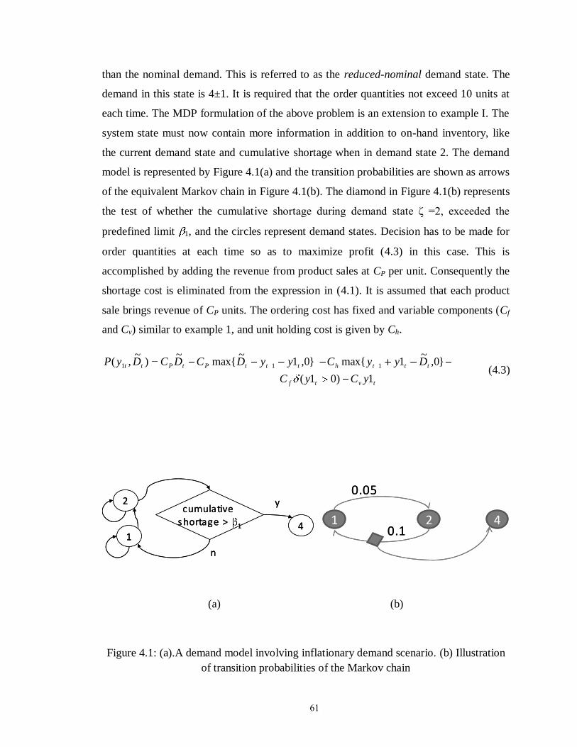
61
than the nominal demand. This is referred to as the reduced-nominal demand state. The
demand in this state is 4±1. It is required that the order quantities not exceed 10 units at
each time. The MDP formulation of the above problem is an extension to example I. The
system state must now contain more information in addition to on-hand inventory, like
the current demand state and cumulative shortage when in demand state 2. The demand
model is represented by Figure 4.1(a) and the transition probabilities are shown as arrows
of the equivalent Markov chain in Figure 4.1(b). The diamond in Figure 4.1(b) represents
the test of whether the cumulative shortage during demand state ζ =2, exceeded the
predefined limit 1, and the circles represent demand states. Decision has to be made for
order quantities at each time so as to maximize profit (4.3) in this case. This is
accomplished by adding the revenue from product sales at CP per unit. Consequently the
shortage cost is eliminated from the expression in (4.1). It is assumed that each product
sale brings revenue of CP units. The ordering cost has fixed and variable components (Cf
and Cv) similar to example 1, and unit holding cost is given by Ch.
tvtf
ttthtttPtPtt
yCyC
DyyCyyDCDCDyP
1)01(
}0,~
1max{}0,1~
max{~
)~
,( 111 (4.3)
1
2cumulative
shortage > 1 4
n
y
1
2cumulative
shortage > 1 4
n
y
1 2 4
0.05
0.11 2 4
0.05
0.1
(a) (b)
Figure 4.1: (a).A demand model involving inflationary demand scenario. (b) Illustration
of transition probabilities of the Markov chain
62
The parameter values are shown in Table 4.1(a) and the optimal policy ( II ) for
the considered parameter values is reported in Table 4.1(b). It turns out that the optimal
policy is still of the parametric form (s,S) and depends on the on-hand inventory and
demand realization but is independent of the cumulative shortage. The optimal policies
pertaining to each individual demand state ( 4,2,1,I ) are also reported. The two
policies are different for ζ =1,2,4, I being the sub-optimal policy for the problem in
example II. 4,2,1,I are obtained by using demand states ζ =1,2 and 4, individually
in example I. It must be noted that 4,2,1, ii
I would be the best possible policy obtained
if the problem in example II was solved using a rolling horizon approach.
1
2
3
cumulative shortage > 1
cumulative inventory > 2
4
n
y
y
reduced order limit
1
2
3
cumulative shortage > 1
cumulative inventory > 2
4
n
y
y
reduced order limit
(a)
1 2 3 4
0.05
0.05
0.10.11 2 3 4
0.05
0.05
0.10.1
(b)
Figure 4.2: (a) A demand model involving inflationary and recessionary demand
scenarios.(b) Illustration of transition probabilities of the Markov chain
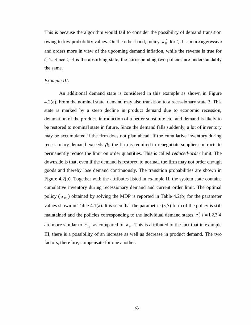
63
This is because the algorithm would fail to consider the possibility of demand transition
owing to low probability values. On the other hand, policy II for ζ=1 is more aggressive
and orders more in view of the upcoming demand inflation, while the reverse is true for
ζ=2. Since ζ=3 is the absorbing state, the corresponding two policies are understandably
the same.
Example III:
An additional demand state is considered in this example as shown in Figure
4.2(a). From the nominal state, demand may also transition to a recessionary state 3. This
state is marked by a steep decline in product demand due to economic recession,
defamation of the product, introduction of a better substitute etc. and demand is likely to
be restored to nominal state in future. Since the demand falls suddenly, a lot of inventory
may be accumulated if the firm does not plan ahead. If the cumulative inventory during
recessionary demand exceeds 2, the firm is required to renegotiate supplier contracts to
permanently reduce the limit on order quantities. This is called reduced-order limit. The
downside is that, even if the demand is restored to normal, the firm may not order enough
goods and thereby lose demand continuously. The transition probabilities are shown in
Figure 4.2(b). Together with the attributes listed in example II, the system state contains
cumulative inventory during recessionary demand and current order limit. The optimal
policy ( III ) obtained by solving the MDP is reported in Table 4.2(b) for the parameter
values shown in Table 4.1(a). It is seen that the parametric (s,S) form of the policy is still
maintained and the policies corresponding to the individual demand states 4,3,2,1ii
I
are more similar to III as compared to II . This is attributed to the fact that in example
III, there is a possibility of an increase as well as decrease in product demand. The two
factors, therefore, compensate for one another.
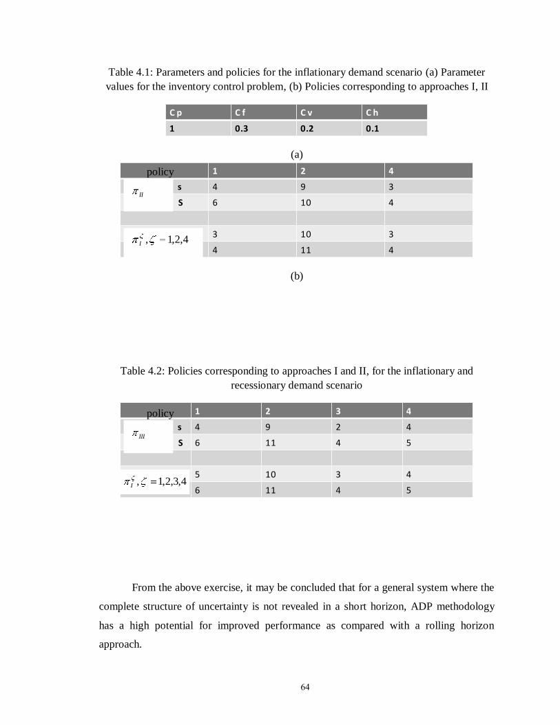
64
Table 4.1: Parameters and policies for the inflationary demand scenario (a) Parameter
values for the inventory control problem, (b) Policies corresponding to approaches I, II
C p C f C v C h
1 0.3 0.2 0.1
C p C f C v C h
1 0.3 0.2 0.1
(a)
1 2 4
C ombined s 4 9 3
-do- S 6 10 4
Independent s 3 10 3
-do- S 4 11 4
1 2 4
C ombined s 4 9 3
-do- S 6 10 4
Independent s 3 10 3
-do- S 4 11 4
(b)
Table 4.2: Policies corresponding to approaches I and II, for the inflationary and
recessionary demand scenario
1 2 3 4
C ombined s 4 9 2 4
-do- S 6 11 4 5
Independent s
5 10 3 4
-do-S
6 11 4 5
1 2 3 4
C ombined s 4 9 2 4
-do- S 6 11 4 5
Independent s
5 10 3 4
-do-S
6 11 4 5
From the above exercise, it may be concluded that for a general system where the
complete structure of uncertainty is not revealed in a short horizon, ADP methodology
has a high potential for improved performance as compared with a rolling horizon
approach.
4,2,1,I
II
III
4,3,2,1,I
policy
policy
65
For the PR problem, the planning level bears more far reaching effects and
therefore calls for rigorous treatment of uncertainty. The formulation of the planning
problem as a MDP is presented in the next section. The reader is referred to Chapter 3 for
problem details and assumptions.
4.2 Formulation of the perishable resource problem as MDP
To be able to successfully formulate the PR problem as MDP, the most important
requirement is the Markov property or the memory-less property. This implies that, the
next state and stage-wise reward must depend only on the current state and action. The
resource life is independent of past decisions and states. Also, since the demand for
products was assumed to have an underlying Markov chain in Chapter 3 and in examples
presented in section 4.1, this condition is met. Finally, for simplicity of illustration, we
opt to formulate the infinite horizon problem which pertains to a stationary optimal
policy. A discount factor γ=0.9 is used in all cases. Demand model is represented by d(ζ)
for general discussion where ζ=1,2,..nD, designates the states of the Markov chain and
d(ζ) the demand associated with that state. Specific demand models are deferred until
section 4.3.3.
4.2.1 MDP formulation
As discussed in Chapter 2, a MDP is characterized by the tuple (S,A,T,R, γ) whose
descriptions in the context of the PR problem are shown below. For consistency,
notational convention is followed from Chapter 3 as much as possible.
State
The state at time t, (st) includes four pieces of information:
(i) Product/stone inventory -xit i=1,2,…nP
(ii) Resource/mold inventory – yijt i=1,2,…nP; j=1,2,... ζT
(iii) Product demand scenario - δt, δt {1,2,..nD}
(iv) Past orders - y1i,t1 i=1, t1= t-1, t-2,…t-l
st = [xit yijt kt y1i,t1] (4.4)
66
dim(st) = nP + nP *max
T + 1 + l (4.5)
|S|= l
D
nnynyx TPP )1()()( maxmaxmax
max
(4.6)
The state description, state dimension and the size of the state space is given by
(4.4), (4.5) and (4.6) respectively. xmax and ymax are externally imposed limits to keep the
problem size finite and ensure that an unreasonable size inventory is not held in the
system. y1max is the upper limit on reorder quantities of the resource and max
T is the
maximum possible resource life.
Action
The actions/decisions are clearly defined in Chapter 3 and classified as planning and
scheduling level decisions. The three types of actions at time t are:
(i) Production quantities - x1it i=1,2,….nP
(ii) Resource reorder - y1it i=1
(iii)Resource transition and allocation - sch
tjiiy ,,1,2 i=1,2...nP; i1=1,2...nP; ; j=1,2,. ζT,
sch
tjjiy ,1,,3 i=1,2...nP; j=1,2,. ζT,,j1=1,2,..,j-1
As outlined in Chapter 3, the production and resource ordering decisions are
planning level decisions while the resource transition and allocation decisions are
determined at the scheduling level in order to best meet the production requirements.
(The time scales t and t’ for the two levels are shown again in Figure 4.3). Therefore,
only the production and resource ordering decisions are considered for the planning
problem. The resource allocation decisions are obtained by solving the scheduling
problem (thereby indicated by suffix sch), a discussion on which is deferred until section
4.3.3. Since only the light molds are ordered at any time, the resource reorder decision
contributes only a single dimension to the decision space.
at = [x1it y1it] (4.7)
dim(at)= 1Pn (4.8)
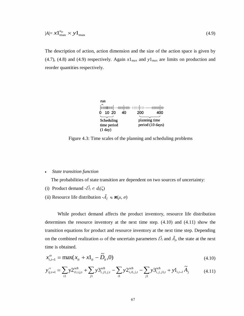
67
|A|= maxmax 11 yx Pn (4.9)
The description of action, action dimension and the size of the action space is given by
(4.7), (4.8) and (4.9) respectively. Again x1max and y1max are limits on production and
reorder quantities respectively.
0 10 20 40 200 400
run
Scheduling
time period
(1 day)
planning time
period (10 days)
0 10 20 40 200 400
run
Scheduling
time period
(1 day)
planning time
period (10 days)
Figure 4.3: Time scales of the planning and scheduling problems
State transition function
The probabilities of state transition are dependent on two sources of uncertainty:
(i) Product demand - i di(ζ)
(ii) Resource life distribution - j (μ, ζ)
While product demand affects the product inventory, resource life distribution
determines the resource inventory at the next time step. (4.10) and (4.11) show the
transition equations for product and resource inventory at the next time step. Depending
on the combined realization ω of the uncertain parameters i and j, the state at the next
time is obtained.
)0,~
1max(1, itititti Dxxx (4.10)
jlti
j
sch
tjji
i
sch
tjii
j
sch
tjji
sch
tij Ayyyyy~
1323y2 ,
1
,1,,
1
,,1,
1
,,1,
i1
tj,i1,i,1, (4.11)
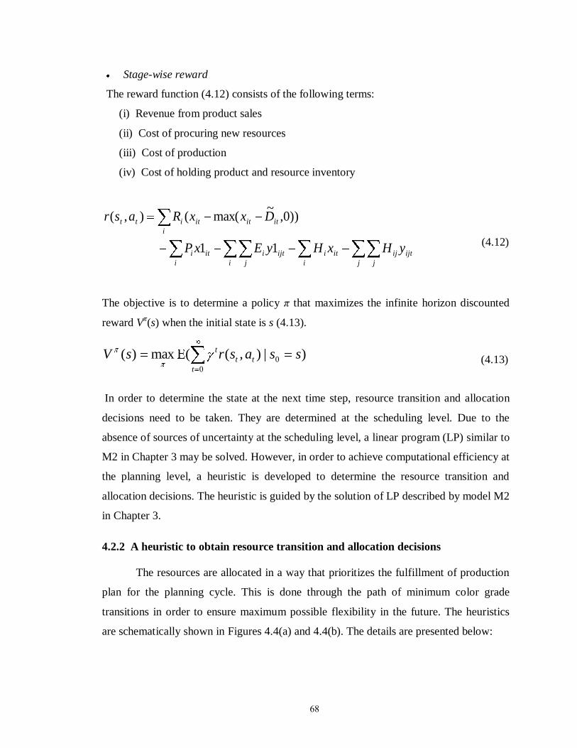
68
Stage-wise reward
The reward function (4.12) consists of the following terms:
(i) Revenue from product sales
(ii) Cost of procuring new resources
(iii) Cost of production
(iv) Cost of holding product and resource inventory
j j
ijtij
i
iti
i j
ijti
i
iti
ititit
i
itt
yHxHyExP
DxxRasr
11
))0,~
max((),(
(4.12)
The objective is to determine a policy π that maximizes the infinite horizon discounted
reward Vπ(s) when the initial state is s (4.13).
)|),((max)(0
0
t
tt
t ssasrsV (4.13)
In order to determine the state at the next time step, resource transition and allocation
decisions need to be taken. They are determined at the scheduling level. Due to the
absence of sources of uncertainty at the scheduling level, a linear program (LP) similar to
M2 in Chapter 3 may be solved. However, in order to achieve computational efficiency at
the planning level, a heuristic is developed to determine the resource transition and
allocation decisions. The heuristic is guided by the solution of LP described by model M2
in Chapter 3.
4.2.2 A heuristic to obtain resource transition and allocation decisions
The resources are allocated in a way that prioritizes the fulfillment of production
plan for the planning cycle. This is done through the path of minimum color grade
transitions in order to ensure maximum possible flexibility in the future. The heuristics
are schematically shown in Figures 4.4(a) and 4.4(b). The details are presented below:
69
The resource transition heuristic
Since it is assumed that only light resource (i=1) can be ordered, resource
transition needs to be performed for production of dark products (i=2). In order to
determine the number of possible transitions, excess light runs, excess_light are
determined at the beginning of the scheduling horizon. Since a resource can be used a
maximum of 10 times (scheduling horizon is 10 days and the resource can be used only
once a day), the number of available runs needs to be adjusted. The adjustment needs to
be made for resources with more than 10 runs remaining. Now, the shortage in dark
resources is determined in terms of number of runs, short_dark. The smaller of the two
quantities, i.e. excess_light and short_dark is scheduled for transition. While
transitioning, the oldest resources are prioritized. This ensures that maximum resource
inventory is held as light resources, imparting flexibility in the future.
The resource usage heuristic
To be able to successfully allocate the resource to production, production
quantities need to be determined at each scheduling time period. The total production
requirement in the given planning period, i.e. x1i, i=1,2 is equally divided into 10 days.
Moreover, the overall fraction of light products, i.e. ν, is maintained during each
scheduling time epoch t′. Having determined the production quantities, resources are
allocated based on newest-first rule. This is because when the resource life distribution is
very uneven, the resources with more number of runs left must be utilized early so as not
to run out of resources.
Having obtained a simple heuristic to determine the state transitions, we analyze
the size of the MDP problem and present an ADP algorithm for its solution in the next
section.
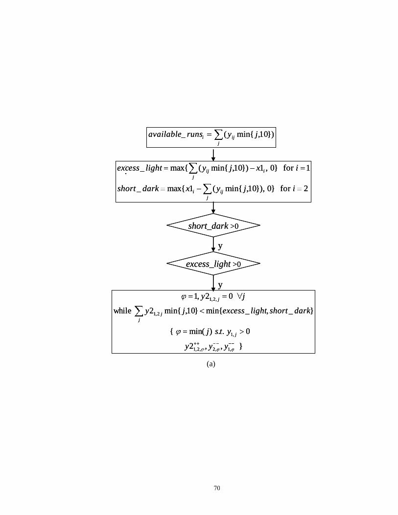
70
j
iji jyrunsavailable })10,min{(_
j
iji
j
iij
ijyxdarkshort
ixjylightexcess
2for}0}),10,min{(1max{_
1for}0,1})10,min{(max{_
short_dark >0
excess_light >0
},,2
0..)min({
}_,_min{}10,min{2while
02,1
,1,2,2,1
,1
2,1
,2,1
yyy
ytsj
darkshortlightexcessjy
jy
j
j
j
j
y
y
j
iji jyrunsavailable })10,min{(_
j
iji
j
iij
ijyxdarkshort
ixjylightexcess
2for}0}),10,min{(1max{_
1for}0,1})10,min{(max{_
short_dark >0
excess_light >0
},,2
0..)min({
}_,_min{}10,min{2while
02,1
,1,2,2,1
,1
2,1
,2,1
yyy
ytsj
darkshortlightexcessjy
jy
j
j
j
j
y
y
(a)
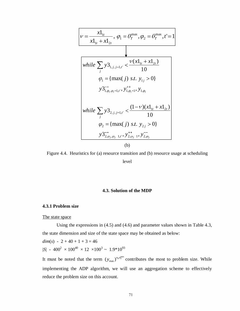
71
1',,,11
1 max
2
max
1
21
1 txx
xTT
tt
t
2222
1111
,21,2',1,,2
22
21',1,,2
,11,1',1,,1
11
21',1,,1
,,3
}0..){max(
10
)11)(1(3
,,3
}0..){max(
10
)11(3
yyy
ytsj
xxywhile
yyy
ytsj
xxywhile
t
j
tttjj
j
t
j
tttjj
j
(b)
Figure 4.4. Heuristics for (a) resource transition and (b) resource usage at scheduling
level
4.3. Solution of the MDP
4.3.1 Problem size
The state space
Using the expressions in (4.5) and (4.6) and parameter values shown in Table 4.3,
the state dimension and size of the state space may be obtained as below:
dim(s) - 2 + 40 + 1 + 3 = 46
|S| - 4002 × 100
40 × 12 ×100
3 ~ 1.9*10
93
It must be noted that the term max
)( maxTPn
y contributes the most to problem size. While
implementing the ADP algorithm, we will use an aggregation scheme to effectively
reduce the problem size on this account.
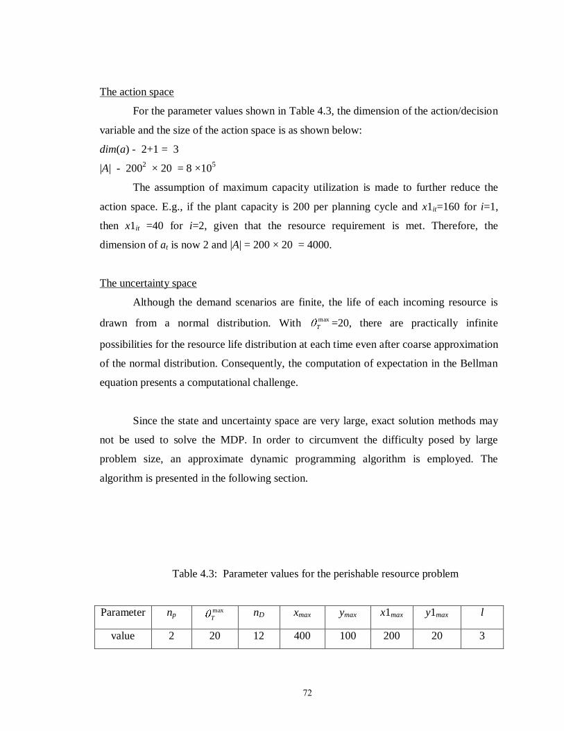
72
The action space
For the parameter values shown in Table 4.3, the dimension of the action/decision
variable and the size of the action space is as shown below:
dim(a) - 2+1 = 3
|A| - 2002 × 20 = 8 ×10
5
The assumption of maximum capacity utilization is made to further reduce the
action space. E.g., if the plant capacity is 200 per planning cycle and x1it=160 for i=1,
then x1it =40 for i=2, given that the resource requirement is met. Therefore, the
dimension of at is now 2 and |A| = 200 × 20 = 4000.
The uncertainty space
Although the demand scenarios are finite, the life of each incoming resource is
drawn from a normal distribution. With max
T =20, there are practically infinite
possibilities for the resource life distribution at each time even after coarse approximation
of the normal distribution. Consequently, the computation of expectation in the Bellman
equation presents a computational challenge.
Since the state and uncertainty space are very large, exact solution methods may
not be used to solve the MDP. In order to circumvent the difficulty posed by large
problem size, an approximate dynamic programming algorithm is employed. The
algorithm is presented in the following section.
Table 4.3: Parameter values for the perishable resource problem
Parameter np max
T nD xmax ymax x1max y1max l
value 2 20 12 400 100 200 20 3
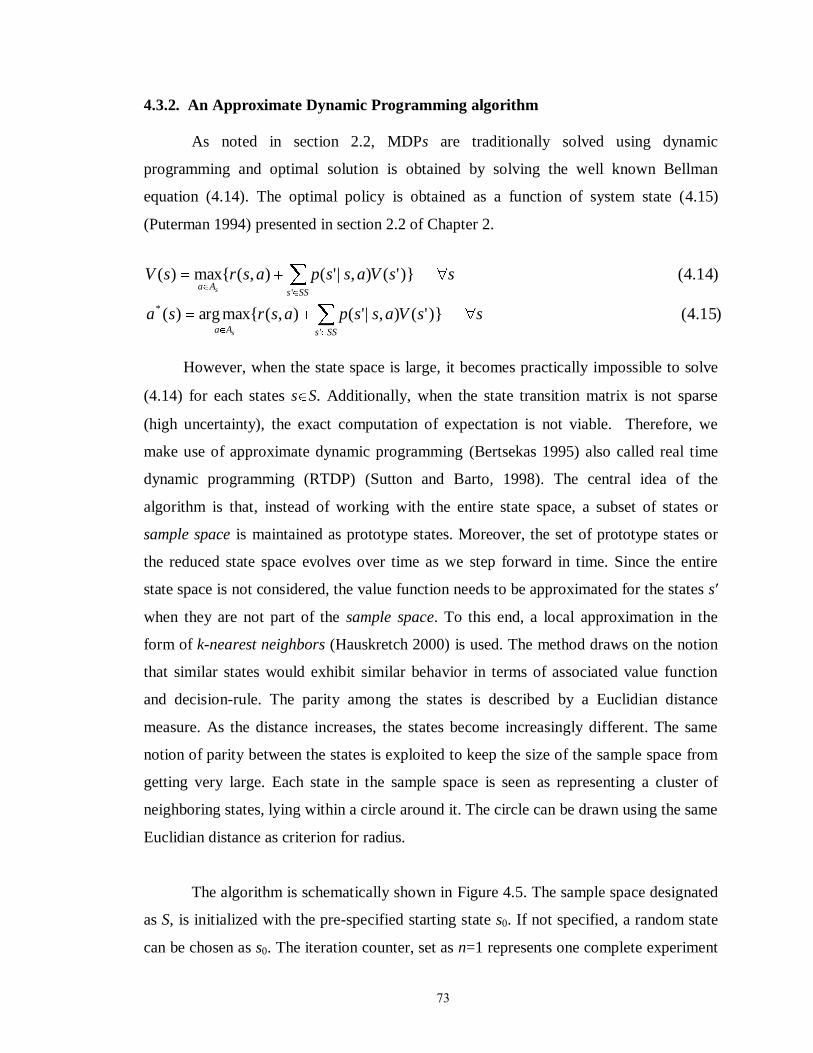
73
4.3.2. An Approximate Dynamic Programming algorithm
As noted in section 2.2, MDPs are traditionally solved using dynamic
programming and optimal solution is obtained by solving the well known Bellman
equation (4.14). The optimal policy is obtained as a function of system state (4.15)
(Puterman 1994) presented in section 2.2 of Chapter 2.
)15.4()}'(),|'(),({maxarg)(
)14.4()}'(),|'(),({max)(
'
*
'
SSsAa
SSsAa
ssVasspasrsa
ssVasspasrsV
s
s
However, when the state space is large, it becomes practically impossible to solve
(4.14) for each states s S. Additionally, when the state transition matrix is not sparse
(high uncertainty), the exact computation of expectation is not viable. Therefore, we
make use of approximate dynamic programming (Bertsekas 1995) also called real time
dynamic programming (RTDP) (Sutton and Barto, 1998). The central idea of the
algorithm is that, instead of working with the entire state space, a subset of states or
sample space is maintained as prototype states. Moreover, the set of prototype states or
the reduced state space evolves over time as we step forward in time. Since the entire
state space is not considered, the value function needs to be approximated for the states s′
when they are not part of the sample space. To this end, a local approximation in the
form of k-nearest neighbors (Hauskretch 2000) is used. The method draws on the notion
that similar states would exhibit similar behavior in terms of associated value function
and decision-rule. The parity among the states is described by a Euclidian distance
measure. As the distance increases, the states become increasingly different. The same
notion of parity between the states is exploited to keep the size of the sample space from
getting very large. Each state in the sample space is seen as representing a cluster of
neighboring states, lying within a circle around it. The circle can be drawn using the same
Euclidian distance as criterion for radius.
The algorithm is schematically shown in Figure 4.5. The sample space designated
as S, is initialized with the pre-specified starting state s0. If not specified, a random state
can be chosen as s0. The iteration counter, set as n=1 represents one complete experiment
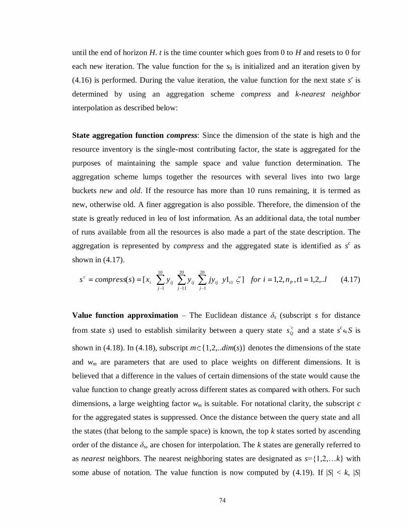
74
until the end of horizon H. t is the time counter which goes from 0 to H and resets to 0 for
each new iteration. The value function for the s0 is initialized and an iteration given by
(4.16) is performed. During the value iteration, the value function for the next state s′ is
determined by using an aggregation scheme compress and k-nearest neighbor
interpolation as described below:
State aggregation function compress: Since the dimension of the state is high and the
resource inventory is the single-most contributing factor, the state is aggregated for the
purposes of maintaining the sample space and value function determination. The
aggregation scheme lumps together the resources with several lives into two large
buckets new and old. If the resource has more than 10 runs remaining, it is termed as
new, otherwise old. A finer aggregation is also possible. Therefore, the dimension of the
state is greatly reduced in leu of lost information. As an additional data, the total number
of runs available from all the resources is also made a part of the state description. The
aggregation is represented by compress and the aggregated state is identified as sc as
shown in (4.17).
ltniforyjyyyxscompresss Pt
j
ij
j
ij
j
iji
c ,..2,11,,2,1]1[)( 1
20
1
20
11
10
1
(4.17)
Value function approximation – The Euclidean distance δs (subscript s for distance
from state s) used to establish similarity between a query state c
Qs ' and a state sc
S is
shown in (4.18). In (4.18), subscript m {1,2,..dim(s)} denotes the dimensions of the state
and wm are parameters that are used to place weights on different dimensions. It is
believed that a difference in the values of certain dimensions of the state would cause the
value function to change greatly across different states as compared with others. For such
dimensions, a large weighting factor wm is suitable. For notational clarity, the subscript c
for the aggregated states is suppressed. Once the distance between the query state and all
the states (that belong to the sample space) is known, the top k states sorted by ascending
order of the distance δs, are chosen for interpolation. The k states are generally referred to
as nearest neighbors. The nearest neighboring states are designated as s={1,2,…k} with
some abuse of notation. The value function is now computed by (4.19). If |S| < k, |S|
75
neighbors are used. Since 01
s
and 11
1
k
s s
, the interpolation is convex and the
contraction map is preserved.
21
)dim(
1
2' ))}()({(s
m
Qms msmsw (4.18)
k
s s
Q
kNN sVsV1
' )(1
)( (4.19)
While attempting to perform the value iteration, the maximization is performed
over all actions in the action space. Since dim(a) is small, a homogenous grid is used to
reduce the size of the action space. E.g., resource order can only occur in multiples of 4
and production is assumed to take place in batches of 10. Additionally, for a state-action
pair, many next states are possible owing to large uncertainty. Since exact computation of
expectation over all possible next states s′ is not possible, sampling methods are used as
described below.
Approximation of expectation: The idea of approximation of expectation is simple.
Starting from s0, for each action a A, samples of next states s′=f(s0,a,ω), ω Ω are
obtained, where Ω is a set of sampled values of uncertain parameters. ω Ω also have
probabilities associated with them. These are designated as pω and are re-normalized to
ensure convergence. The value iteration update based on sampled uncertainty is shown in
(4.20)
}),|(
),,((),|(
),({max)(ˆ1
asp
asfVasp
asrsVn
Aan
s
(4.20)
In Figure 4.5, the approximation is illustrated for only one sample realization of the
uncertainty. Higher number of samples helps convergence.
76
After the value iteration update, one or a set of maximizing actions a* are obtained. a
* is
the best action for state s0 based on the knowledge so far. However, because of the
approximation of expectation mentioned above, the value function is a biased estimate of
the mean discounted reward. Also, since all the states in the sample space are not updated
during one iteration, exploration needs to be performed to access different parts of the
original state space. This is accomplished by perturbing the action around the best known
action a*. This is described below.
Exploration v/s exploitation: The perturbation in the action is performed by using
a*+Δa
{n} instead of a
* to move forward in time. The perturbation Δa
{n} is dependent on
the iteration counter n. At the beginning of the algorithm, the value function estimates are
poor and very few states are a part of the sample space for successful interpolation and
good representation of the original state space. This is the reason why higher degree of
perturbation in action is needed. As the number of iterations increase, Δa is dampened to
be able to exploit the information obtained so far. The specific form of Δa used for the
PR problem is shown in (4.21). q represents a general quantity, e.g., production and
reorder, λ1 (0,1], λ2>0 are parameters and qmax is the maximum possible value of q. For
the perishable resource application λ1=0.4 and λ2=1.5 are used.
nqqq 2)( max1
* (4.21)
Having performed the value iteration update for the initial state s0, and obtained
the perturbed action a*+Δa
{n} , next state s1 is obtained by taking one sample realization
of the uncertainty ω1. In usual practice a sample trajectory for the experiment, i.e.,
ω1,ω2,..ωH is generated a priori. At this point, it needs to be determined whether cs1 must
be admitted to the sample space.
Conditional admittance to sample space - The next statecs1 is not admitted if it has
enough representation in the sample space, i.e. there is at least one state in the sample
space, that is similar tocs1 . The state is referred to as an alias. An alias is also determined
based on the distance criterion seen in (4.18). A neighbor is called an alias if its distance
77
from the query point is below a pre-defined threshold δmax
(4.22). Having obtained s1, the
time counter is increased and the iteration is repeated. If s1 was admitted to the sample
space in the previous iteration, its value function would be assigned by the next value
iteration. Otherwise, the aliases are used as s1 for updating the value function. A small
value of δmax
would result in a very large state space whereas a large value of δmax
would
result in poor representation of the relevant state space by the sample space. Therefore,
δmax
is an important parameter which must be chosen carefully.
}),(:{)( maxssssalias QQ (4.22)
As pointed out earlier, the value function estimate obtained after value iteration is a
biased of the true mean, a smoothing parameter αε is used.
Value function smoothing - This technique essentially determines a moving average
estimate of the value function V(sc) s
cS. Represented by (4.23), the value function
update at the nth
iteration is obtained as a convex combination of the old and new values.
The smoothing factors 10 are generally different for each state in that they
depend on the number of times the corresponding state has been visited (designated by
ε{s}
). Therefore ε{s}
needs to be stored for each state sc
S. In order to strike the balance
between exploration and exploitation, much the same way as with the action, αε must be
dampened with time as well. Expression (4.24) is used to achieve the same with λ3=20 for
the perishable resource problem.
)( 3
3 (4.24)
When the incumbent state does not belong to the state space, the aliases are used
for value function update. The iteration is repeated until either the computational limit is
reached or the value function convergence criterion is met.

78
Step 0. Set n=1, define the starting state s0,
1)(),(initialize,set),( 00000
cccc ssVsSscompresss
Step 1. Set t=0, determine a sample path ω1, ω2,.. ,ωH
Step 2. ),,(' determine, tta asfsAa
ascompresss a
c
a )'('
Step 3a. )'(determine,'if , c
a
c
a sVSsa
))(()'(else SsVKNNsV cc
a
Step 3b. )}'(),({max)( c
atAa
c
t sVasrsv
)}'(),({maxarg* c
atAa
sVasra
Step 4. ,If Ss c
t
)()()1()( c
t
c
t
c
t svsVsV (4.23)
1)()( c
t
c
t ss
)(elseif c
tsalias
)()()()1()( c
t
c
t saliasssvsVsV
)(1)()( c
tsaliassss
else
1)(),()(, c
t
c
t
c
t
c
t ssvsVStosadd
Step 5. If t<H,
VVasfsaaa ttttt ),,,( , 1
*
set t=t+1 and go to Step 6
else go to Step 1
Step 6. If n<N, set n=n+1 and go to Step 1
else Stop
Figure 4.5: An approximate dynamic programming algorithm

79
The number of states as a function of iteration count n is shown in Figure 4.6(a)
for a particular demand model (described in the next section). Selected states are added as
they are encountered during each iteration. More states are added in the initial iterations
and the number of new states to be added to the sample space dwindles as the sample
space becomes a good representation of the relevant state space. A good strategy is to
start with a high value of δ and keep reducing it until the performance for two successive
values is comparable. Really high values of δ result in very few states in the sample space
as seen in Figure 4.6(a). Also, the convergence of the value function for some of the most
visited states is shown in Figure 4.6(b). Depending on the initialization, the value
function either trends upwards or downwards and finally converges after sufficient
number of iterations.
4.3.3. Demand modeling revisited
Three different demand models are considered:
(i) Deterministic demand- The seasonal demand pattern (4.25) used in Chapter 3
(section 3.4) is used. The demand pattern (4.25) in assumed to repeat until t , while
counter τ=1,2,..30 is included in the state definition. The counter resets to 1 after τ=30.
3021]100100[
2011]140140[
101]6060[
)(
if
if
if
d sea (4.25)
While implementing the ADP algorithm shown in Figure 4.5, for the
deterministic problem, the smoothing operation (4.23) is not needed. This is because of
the absence of uncertainty leading to exact value update for every state. The action is still
perturbed to counter the effects of dicretization.
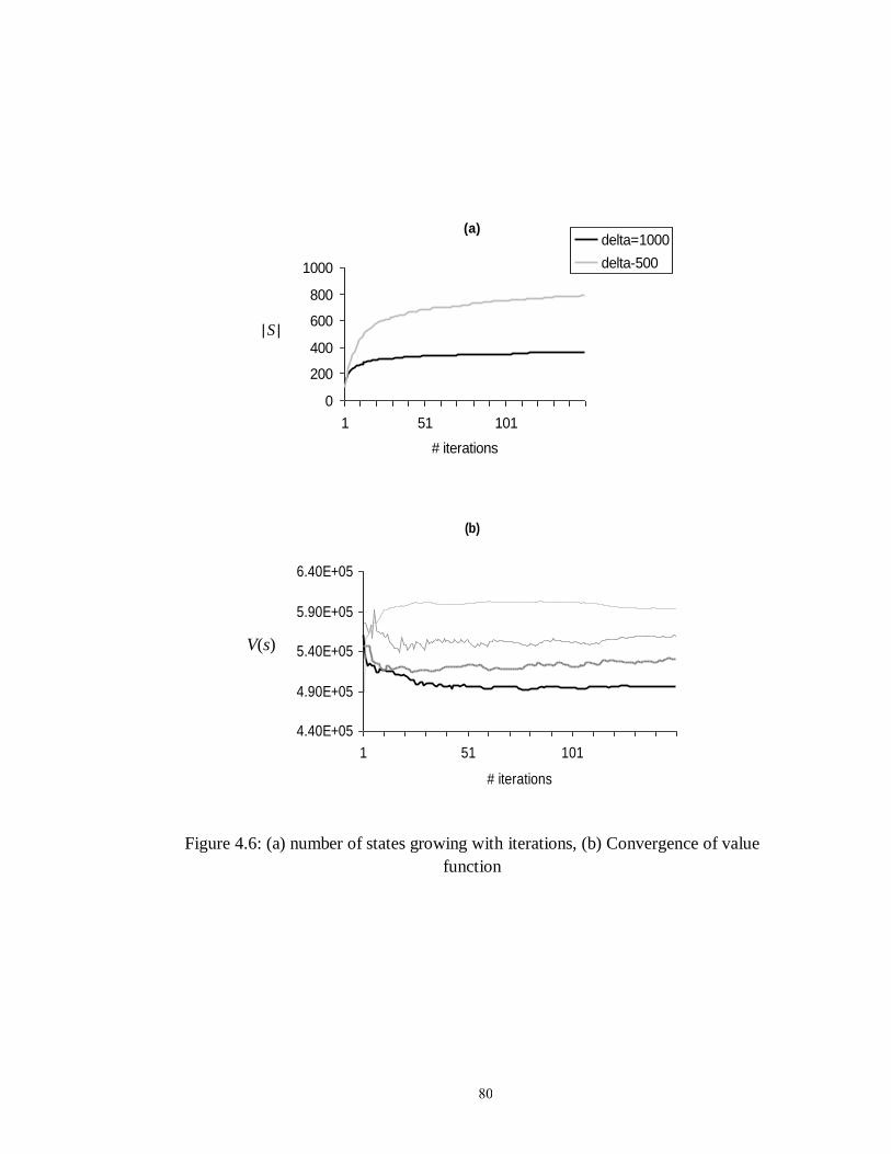
80
(a)
0
200
400
600
800
1000
1 51 101
# iterations
|S|
delta=1000
delta-500
(b)
4.40E+05
4.90E+05
5.40E+05
5.90E+05
6.40E+05
1 51 101
# iterations
V(s
)
Figure 4.6: (a) number of states growing with iterations, (b) Convergence of value
function
|S|
V(s)
81
(ii) Demand with fluctuations around a constant mean
Similar to Chapter 3, the stochasticity in demand is modeled as a Markov chain
with twelve states shown in Table 4.4. These states represent deviations from nominal
demand for the light and dark products. The transition probabilities pertaining to low,
medium and high cases of uncertainty are given by T1 (4.26), T2 (4.27) and T3 (4.28)
respectively.
otherwise
andif
andif
T
0
4''3
2.0
4''8.0
)',(1 (4.26)
otherwise
andif
andif
T
0
8''7
2.0
8''8.0
)',(2 (4.27)
otherwise
if
T
11
2.0
'8.0
)',(3 (4.28)
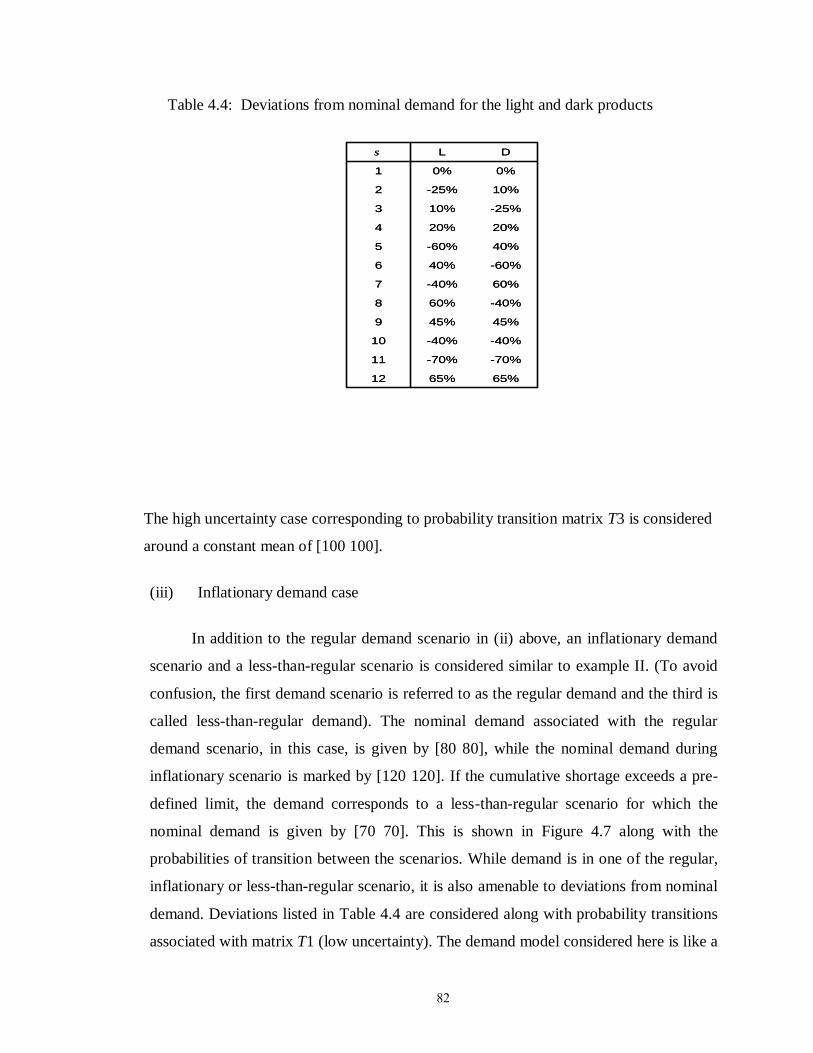
82
Table 4.4: Deviations from nominal demand for the light and dark products
65%65%12
-70%-70%11
-40%-40%10
45%45%9
-40%60%8
60%-40%7
-60%40%6
40%-60%5
20%20%4
-25%10%3
10%-25%2
0%0%1
DLs
65%65%12
-70%-70%11
-40%-40%10
45%45%9
-40%60%8
60%-40%7
-60%40%6
40%-60%5
20%20%4
-25%10%3
10%-25%2
0%0%1
DLs
The high uncertainty case corresponding to probability transition matrix T3 is considered
around a constant mean of [100 100].
(iii) Inflationary demand case
In addition to the regular demand scenario in (ii) above, an inflationary demand
scenario and a less-than-regular scenario is considered similar to example II. (To avoid
confusion, the first demand scenario is referred to as the regular demand and the third is
called less-than-regular demand). The nominal demand associated with the regular
demand scenario, in this case, is given by [80 80], while the nominal demand during
inflationary scenario is marked by [120 120]. If the cumulative shortage exceeds a pre-
defined limit, the demand corresponds to a less-than-regular scenario for which the
nominal demand is given by [70 70]. This is shown in Figure 4.7 along with the
probabilities of transition between the scenarios. While demand is in one of the regular,
inflationary or less-than-regular scenario, it is also amenable to deviations from nominal
demand. Deviations listed in Table 4.4 are considered along with probability transitions
associated with matrix T1 (low uncertainty). The demand model considered here is like a
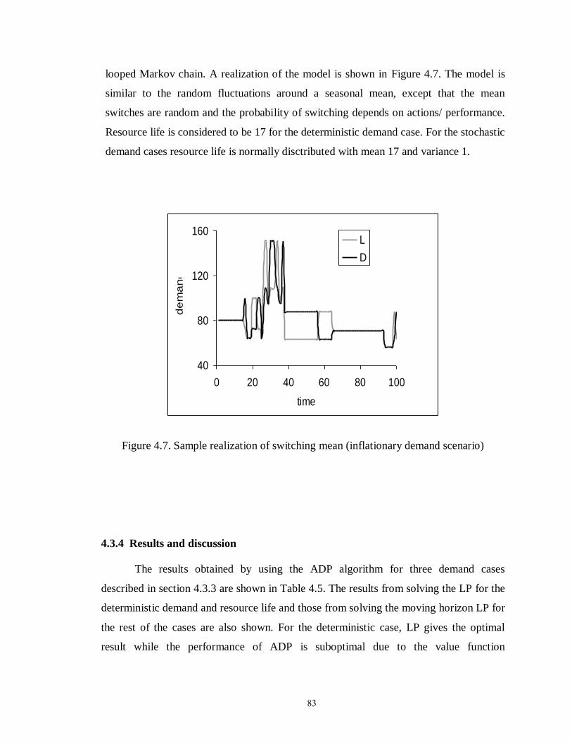
83
looped Markov chain. A realization of the model is shown in Figure 4.7. The model is
similar to the random fluctuations around a seasonal mean, except that the mean
switches are random and the probability of switching depends on actions/ performance.
Resource life is considered to be 17 for the deterministic demand case. For the stochastic
demand cases resource life is normally disctributed with mean 17 and variance 1.
40
80
120
160
0 20 40 60 80 100
time
de
ma
nd
L
D
Figure 4.7. Sample realization of switching mean (inflationary demand scenario)
4.3.4 Results and discussion
The results obtained by using the ADP algorithm for three demand cases
described in section 4.3.3 are shown in Table 4.5. The results from solving the LP for the
deterministic demand and resource life and those from solving the moving horizon LP for
the rest of the cases are also shown. For the deterministic case, LP gives the optimal
result while the performance of ADP is suboptimal due to the value function
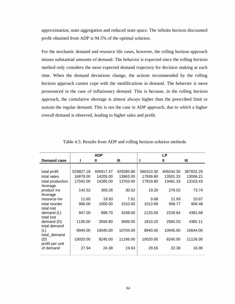
84
approximation, state aggregation and reduced state space. The infinite horizon discounted
profit obtained from ADP is 94.5% of the optimal solution.
For the stochastic demand and resource life cases, however, the rolling horizon approach
misses substantial amounts of demand. The behavior is expected since the rolling horizon
method only considers the most expected demand trajectory for decision making at each
time. When the demand deviations change, the actions recommended by the rolling
horizon approach cannot cope with the modifications in demand. The behavior is more
pronounced in the case of inflationary demand. This is because, in the rolling horizon
approach, the cumulative shortage is almost always higher than the prescribed limit to
sustain the regular demand. This is not the case in ADP approach, due to which a higher
overall demand is observed, leading to higher sales and profit.
Table 4.5: Results from ADP and rolling horizon solution methods
ADP LP
Demand case I II III I II III
total profit 529827.18 445917.47 429285.89 560310.30 409244.30 367832.29
total sales 16878.00 14205.00 13963.00 17939.80 13501.33 13006.21
total production 17042.00 14285.00 13763.00 17919.80 13481.33 13103.43 Average product inv 142.52 300.26 30.52 19.20 276.02 73.74 Average resource inv 11.65 19.93 7.91 9.68 21.93 10.67
total reorder 996.00 1006.00 1010.00 1013.99 908.77 906.48 total lost demand (L) 947.00 898.70 4208.00 2120.00 2228.64 4381.68 total lost demand (D) 1135.00 3594.80 3699.00 1810.20 2560.03 4382.11 total demand (L) 8940.00 10045.00 10704.00 8940.00 10045.00 10644.00 total_demand (D) 10020.00 8245.00 11166.00 10020.00 8245.00 11126.00 profit per unit of demand 27.94 24.38 19.63 29.55 22.38 16.90
85
4.4 Conclusions
An alternative approach to solving the planning and scheduling problems with
perishable resources is presented in this chapter. Due to absence of uncertainty at the
scheduling level, the decisions are determined by heuristics for resource transition and
allocation. These heuristics are guided by the solution of LP which was formulated in
Chapter 3. For the solution of the large sized planning problem, an approximate dynamic
programming algorithm is presented. For the deterministic problem and for the parameter
set considered, the solution obtained by the ADP algorithm is 94.5% of the optimal
solution.
Two models are considered to account for uncertainty in demand and resource
life. While resource life is drawn from a normal distribution, the demand is modeled to
randomly deviate (i) from a constant mean and (ii) from a randomly switching mean. The
probability of mean switching in case (ii) is dependent on current state and action. It is
observed that for both the stochastic demand models, the ADP algorithm produces
substantially better solutions as compared with the rolling horizon approach. This is
because the form of the uncertainty cannot be successfully captured using the rolling
horizon approach. Additionally when mean switching depends on the performance, poor
decision-making has a more far reaching effect on overall performance.
86
CHAPTER 5
HANDLING DEFECT PROPAGATION IN SYSTEMS WITH
STATIONARY EQUIPMENT AND COSTLY JOB INSPECTION
5.1 Introduction
Many manufacturing systems have large machines/ equipment that deteriorate
randomly. Examples can be seen in auto-parts manufacturing, semi-conductor
manufacturing, chemical process industry, etc. The effect of this deterioration is generally
reflected in one or a combination of the following: lower yield, higher fraction of
defective intermediates, higher operating or maintenance cost, or increased probability of
complete failure of the equipment. The random deterioration in a single machine is often
modeled as a Markov chain (Osaki 2002), where the equipment can be in one of N states
at any time. State is designated as i=1,2,…,N, with 1 being the best state and the machine
progressively degrading until it reaches an absorbing state N. The state N may
characterize a completely failed state or a state of worst possible machine performance
leading to least economically favorable production scenario. The states 1,2,…N are rarely
known to the decision-maker and the machine may end up in state N (failed), without
decision-maker‟s notice termed as „silent failures‟ in (Ivy and Polak, 2005).
To keep the machine from ending up in a failed state, an optimal maintenance
policy is needed. Typical decisions include renewal/ replacement (bring the machine back
to the state 1), repair (bring it back to a relatively newer state), machine inspection (incur
a cost to know the machine condition), or inspection of machine‟s output. The inspection
is needed because the machine condition is not directly observable and may lead to
perfect or imperfect knowledge of the condition depending on the quality of observations.
Xiong et al, (2002) present a survey on replacement and repair policies for randomly
deteriorating systems found in existing literature and industry. Typical policy structures
are block replacement, age replacement, order replacement, failure limit policy,
sequential preventive maintenance policy, and repair cost limit policy. A more rigorous
approach, introduced by Girshick (1952) is to use a Partially Observable Markov
87
Decision Process (POMDP) framework to obtain an optimal repair and inspection policy.
To this end, a survey of maintenance studies on single machine systems prone to
stochastic degradation is given in Pierskalla and Voelker, (1976); Monahan (1982).
Structural properties of the optimal value function and optimal policies are derived for
many cases.
A case of particular interest is the one where the machine deterioration is reflected
in increased production of defective jobs considered by Smallwood and Sondik (1973).
The information about the machine condition may be known only by means of costly
inspection of the machine output which relates probabilistically to the machine condition.
The problem of costly job inspection is considered by Smallwood and Sondik, (1973);
Ehrenfeld (1976); White (1979); Monahan (1980), and is referred to as the case with
„imperfect and incomplete observation‟. Due to high cost of inspection, it may not be
economically favorable to test every processed job. Such characteristics are prevalent in
jobs requiring specialized testing for quality variables like electrical properties,
radioactivity, product composition, uniformity, etc.
In most real world situations, a job undergoes a series of operations on multiple
machines. Therefore, the notion of incomplete job inspection motivates the analysis of
defect accumulation and propagation in systems with multiple operations and (or)
multiple machines. This is because the untested defective intermediates would propagate
through the system, until found defective in the final testing. Due to the possibility of
accumulation of defective intermediates, job scheduling may also be affected by machine
renewal and job inspection decisions. It should be noted that even if the inspection of all
jobs was favorable, in the presence of inspection errors of type I (Lee and Unnikrishnan,
1998), defective jobs would be reported as non-defective and allowed to propagate
through the system. Only error-free or perfect inspection is considered in this work but
the analysis can be easily extended to type I errors. The above mentioned aspects of
defect accumulation and propagation in systems with stochastically degrading machine(s)
are addressed by considering two process flow topologies:
88
(i) a re-entrant flow system characterized by a job going through the same operation
more than once
(ii) a hybrid flow system which is a combination of serial and re-entrant flow
Since the knowledge of the deterioration level of the machine(s) and the un-tested
defective jobs is not completely available, the problems are formulated as POMDP.
However, addition of scheduling decisions in the presence of partially observable states
leads to fairly large size problems even for simple real world systems. Fortunately, recent
research (Pineau et al, 2003; Smith and Simmons 2004; Spaan and Vlassis, 2005) in the
area of approximate solution methods for large POMDPs proves helpful in this regard. A
point based solution method called Perseus (Spaan and Vlassis, 2005) is used to solve the
above-mentioned problems and the experimental results are reported. Comparison with
prevailing periodic policies for maintenance and inspection are also presented.
5.2 System Description
In this work, discrete manufacturing systems with single or multiple machines are
considered. The general characteristics of the system and modeling assumptions are as
follows:
5.2.1 Modeling machine deterioration
All machines considered in subsequent problems are modeled to be deteriorating
according to an underlying Markov chain. A good state is differentiated from a bad state
by the associated probability of defect generation βs, such that βs < βs+1 for s=1,2…N-1.
Actions of machine renewal, job inspection and job scheduling are considered. The
processed job is observed to be either defective or non-defective with complete accuracy
whenever job inspection is performed. In case of multiple machine systems, the state
transition probabilities and defect probabilities corresponding to machine states are
independent from one machine to another unless otherwise mentioned.
5.2.2 Defect accumulation and propagation
It is assumed that a defective job can be scrapped or reworked (depending on the
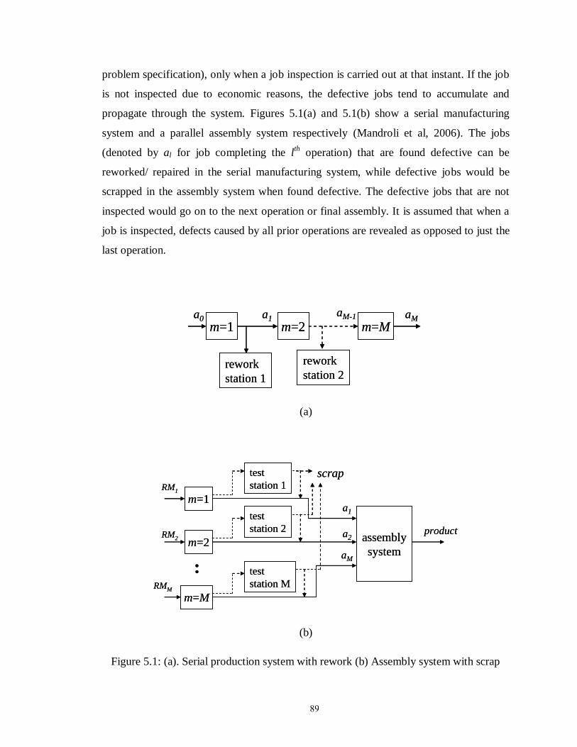
89
problem specification), only when a job inspection is carried out at that instant. If the job
is not inspected due to economic reasons, the defective jobs tend to accumulate and
propagate through the system. Figures 5.1(a) and 5.1(b) show a serial manufacturing
system and a parallel assembly system respectively (Mandroli et al, 2006). The jobs
(denoted by al for job completing the lth
operation) that are found defective can be
reworked/ repaired in the serial manufacturing system, while defective jobs would be
scrapped in the assembly system when found defective. The defective jobs that are not
inspected would go on to the next operation or final assembly. It is assumed that when a
job is inspected, defects caused by all prior operations are revealed as opposed to just the
last operation.
m=1 m=2 m=M
rework
station 1
rework
station 2
a0 a1aM-1 aM
m=1 m=2 m=M
rework
station 1
rework
station 2
a0 a1aM-1 aM
(a)
m=1
m=2
m=M
test
station 1
test
station 2
test
station M
assembly
system
scrap
a1
a2
aM
RM1
RM2
RMM
product
m=1
m=2
m=M
test
station 1
test
station 2
test
station M
assembly
system
scrap
a1
a2
aM
RM1
RM2
RMM
product
(b)
Figure 5.1: (a). Serial production system with rework (b) Assembly system with scrap
90
For the purpose of modeling, the defective jobs in the system need to be kept
track of at all time. Therefore, at any time, the system state can be fully characterized by
two pieces of information: (i) the state of all the machines (ii) the total number of
intermediates and the fraction of defective items in them. To differentiate the general
system state from machine state, the latter is referred by machine condition or
deterioration level in subsequent analysis.
5.2.3. Objective
Most studies on optimal maintenance policies for randomly deteriorating systems
minimize the finite or infinite horizon cost (Smallwood and Sondik, 1973; Osaki 2002;
Ivy and Polak, 2005). This is because the degradation of the machine is reflected in
increasing operating cost and/or increasing maintenance cost as the machine regime gets
worse. For example in (Ivy and Polak 2005), the cost of repair increases with the extent
of repair, which in turn depends on how severe is the deterioration. In this work, it is
assumed that the cost of renewal is the same for all machine regimes. Since inspection is
carried out on jobs only, inspection cost is not a function of machine regime.
Consequently, the deterioration is only reflected in the fraction of defective jobs, an
increase in which leads to lower revenue. Therefore, the infinite horizon profit is
maximized for all illustrations.
A good heuristic used in industrial applications is to employ an age
replacement/renewal policy and periodic inspection policy. In similar spirit, heuristics of
the following nature are used to establish a lower bound on the POMDP solution.
- maintain every ζm time units
- test every ζt time units
The best periodic policy also helps to obtain a sample set of belief points
representing the relevant region for carrying out PERSEUS iterations. The FOMDP
solution provides a loose and unachievable theoretical upper bound.
5.2.4. The single machine system
For a single machine prone to random degradation, the following cases have been
extensively studied:
91
Fully observable – the machine state is perfectly observable
Unobservable – no information about the machine condition is available at any time
Imperfect observation – imperfect observations e.g. information about processed job
is readily available at all times
Costly inspections – machine inspection or job inspection may be carried out at a
cost.
For all of the above cases (Derman 1963; White 1979; Monahan 1980) have proven
the existence of optimal control limit policies under certain assumptions on the system
dynamics and reward function. A particular instance is the unobservable case where the
optimal policy is to replace every m runs, where m can be infinity (Derman 1963). The
conditions for such a policy to be optimal are:
( ) ( , ) is nonincreasing in
( ) For an ordering '
( , ') ( , ) is monotonein
( ) is nondecreasing in for , {1,2,.. }N
ij
j k
i r s a s a
ii a a
r s a r s a s
iii p i a k N
In order to understand the concept of partial and incomplete observation and lay
the foundation for future illustrations, an instance of the „general repair and inspect ion
model‟ presented in (Monahan 1982) is shown as illustration I. For ease of exposition, the
transition probability matrix is considered to be an upper triangular matrix for all actions
except that of machine renewal. This requires that pij =0 for i<j and pNN = 1, making s=N
an absorbing state. The transition probabilities corresponding to the renewal action have
pi1 =1, pij=0, j 1.
Illustration I: A hypothetical machine produces one job per unit time and is prone to
deterioration according to the model described earlier in this section. Pertinent decisions
include machine renewal and job inspection, both of which are assumed to be
instantaneous and have associated costs CM and CI respectively. The machine may
transition to a different deterioration level at each time. Degradation time-scales are
therefore controlled by the probability transition matrix corresponding to the action(s) of
92
non-renewal. A reward CP is received only if the processed job is non-defective (which is
determined for all jobs during final testing before product sale).
S ={1,2,.. ,N}
A ={a1,a2,a3}: a1 - do nothing; a2 - inspect; a3 - renew
O={o1,o2,o3}: o1- no defect; o2 - defect; o3 - no observation
R(s,a,s’) = (1- s’)CP-IM(a)CM-II(a)CI
Oa2(o1|s’) = 1- s’ ; Oa2(o2|s’) = s’
Oa(o1|s’) = 1 for a a2
where, IM(a) and II(a) are binary numbers equal to 1 when the machine is renewed and
job inspection is performed respectively. The POMDP for N=3 (three levels of
deterioration) with CP = 1000, CM = 10000 and three different values of CI (parameter
sets 1,2 and 3 shown in Table 5.1), is solved using PERSEUS (as discussed in Section 2.3
of Chapter 2) and the optimal policy structure is shown in Figure 5.2 (for CI =150). It is
seen that the optimal policy has a control limit structure due to the following system
properties.
aasopasopiv
ssforasopasopiii
NsforaNspasspii
ssforasrasri
),1|(),1|()(
10),1|(),|()(
'0),|'(),|'()(
10),1(),()(
21
11
The policy can therefore be compactly represented as (5.1) for the above
parameter values. It can be shown that a general system with N-state deterioration and
above properties satisfies the monotonicity properties shown by (Monahan 1982). Those
noted above represent sufficient conditions for monotonicity results to hold. This is
demonstrated in appendices A through C.
otherwisejobinspect
bbifrenew
bifnothingdo
policy 1)1(2)3(3
4
09.0)3(
(5.1)
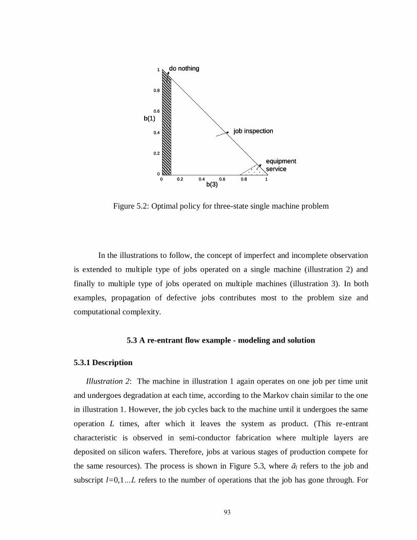
93
0 0.2 0.4 0.6 0.8 1
1
0.8
0.6
0.4
0.2
0
b(3)
b(1)
do nothing
job inspection
equipment
service
0 0.2 0.4 0.6 0.8 1
1
0.8
0.6
0.4
0.2
0
b(3)
b(1)
do nothing
job inspection
equipment
service
Figure 5.2: Optimal policy for three-state single machine problem
In the illustrations to follow, the concept of imperfect and incomplete observation
is extended to multiple type of jobs operated on a single machine (illustration 2) and
finally to multiple type of jobs operated on multiple machines (illustration 3). In both
examples, propagation of defective jobs contributes most to the problem size and
computational complexity.
5.3 A re-entrant flow example - modeling and solution
5.3.1 Description
Illustration 2: The machine in illustration 1 again operates on one job per time unit
and undergoes degradation at each time, according to the Markov chain similar to the one
in illustration 1. However, the job cycles back to the machine until it undergoes the same
operation L times, after which it leaves the system as product. (This re-entrant
characteristic is observed in semi-conductor fabrication where multiple layers are
deposited on silicon wafers. Therefore, jobs at various stages of production compete for
the same resources). The process is shown in Figure 5.3, where l refers to the job and
subscript l=0,1…L refers to the number of operations that the job has gone through. For
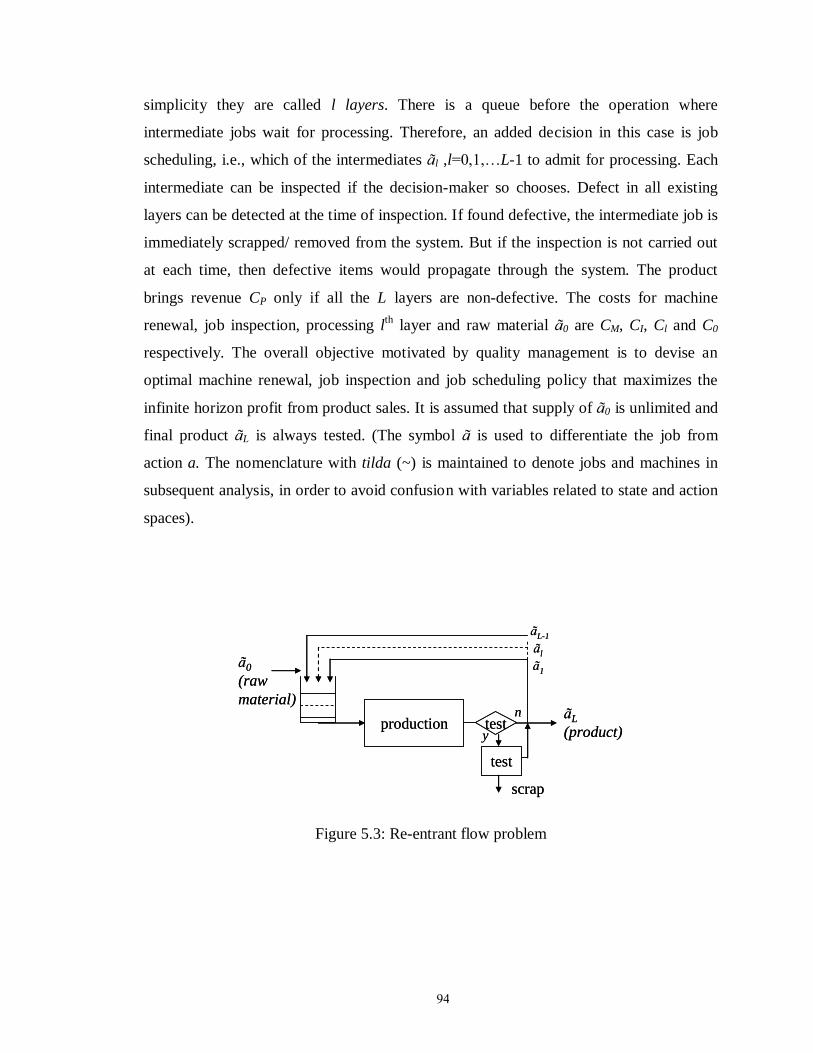
94
simplicity they are called l layers. There is a queue before the operation where
intermediate jobs wait for processing. Therefore, an added decision in this case is job
scheduling, i.e., which of the intermediates l ,l=0,1,…L-1 to admit for processing. Each
intermediate can be inspected if the decision-maker so chooses. Defect in all existing
layers can be detected at the time of inspection. If found defective, the intermediate job is
immediately scrapped/ removed from the system. But if the inspection is not carried out
at each time, then defective items would propagate through the system. The product
brings revenue CP only if all the L layers are non-defective. The costs for machine
renewal, job inspection, processing lth
layer and raw material 0 are CM, CI, Cl and C0
respectively. The overall objective motivated by quality management is to devise an
optimal machine renewal, job inspection and job scheduling policy that maximizes the
infinite horizon profit from product sales. It is assumed that supply of 0 is unlimited and
final product L is always tested. (The symbol is used to differentiate the job from
action a. The nomenclature with tilda (~) is maintained to denote jobs and machines in
subsequent analysis, in order to avoid confusion with variables related to state and action
spaces).
production
test
scrap
aL
(product)
a1
al
aL-1
a0
(raw
material)
testy
nproduction
test
scrap
aL
(product)
a1
al
aL-1
a0
(raw
material)
testy
n
Figure 5.3: Re-entrant flow problem
95
The above problem is interesting in the following ways:
i. It allows for analysis of the propagation and accumulation of defective jobs by
means of a compact system representation.
ii. For very small and very large queue sizes, the system would behave as a serial
production (Figure 5.1(a)) and assembly system (Figure 5.1(b)) respectively. For
example, when no jobs are allowed to wait in the queue, one job remains in the
system until completion. This is similar to the job going through a sequence of L
operations in a series. On the other hand, if a large number of intermediates are
waiting in the queue for processing, then it acts more like an assembly system.
iii. Job inspection now serves two purposes, i.e., it not only provides information
about the machine degradation, but also gives information about defective
intermediates so that they can be picked out of the system to save the cost of
additional operation on them.
iv. The job gathers value with each deposited layer. With better inspection and job
scheduling, it is possible to reduce the number of good layers lost on bad
products. This is because, a product is considered defective if at least one layer on
it is defective.
Similar to the previous illustration, the system is modeled as a POMDP. The
modeling details are included in the formulation and examples are presented for a three
layer product, i.e. for L=3. The problem is referred to as the re-entrant flow problem. It is
worth noticing that the state dimension and consequently, the size of the state space are
significantly larger in this case. This is because now the total number of intermediates in
the system and the fraction of defective intermediates need to be accounted for. The
action space has an added dimension of job scheduling and the state transition probability
matrix also takes into account the probability of defect propagation.
96
5.3.2 Formulation as POMDP
State
The system at any time is fully characterized by the total number of jobs, the fraction of
defective jobs and the deterioration level of the machine. Therefore,
s = [n1 n2 ...nL-1 d1 d2 ...dL-1 ]
nl {0,1,2.., }- total number of l in the queue for l=1,2..L-1
dl {0,1,2..,nl} - number of defective l in the queue for l=1,2..L-1
{1,2..,N}- discrete integer representing the deterioration level of the machine
The state space consists of all possible combinations of the above parameters. For
instance, if L=3 and if the maximum allowable number of jobs in the queue ( ) is limited
to 3 (i.e., n1 + n2 ≤3), then there are following (n1,n2) combinations: (3,0) (2,1) (1,2) (0,3)
(2,0) (1,1) (0,2) (1,0) (0,1) (0,0). For a particular value of n1 say 3, d1 can hold four
possible values from 0,1,2,3. Therefore, the total number of possible combinations for [n1
n2 d1 d2] is 35. With 3 deterioration levels for the machine, the size of the state space is
105 (35 × 3). Similarly, the size of the state space for maximum queue sizes of 4 and 5
are 210 and 378 respectively.
Action/ Decision
a = [ a1 a2 a3]
where a1 {0,1,2,..L-1} pertains to the job scheduling decision (admit 0 , 1 … L-1) ; a2
{0,1} pertains to job inspection decision (test (1) the processed job or not (0)) ;
a3 {0,1} pertains to renewal decision (renew the machine(1) or not (0)). Assuming all
final products are tested, the size of action space for L=3 is ((3 x 2)-1) x 2 = 10.
Observation
o {o1,o2,o3}
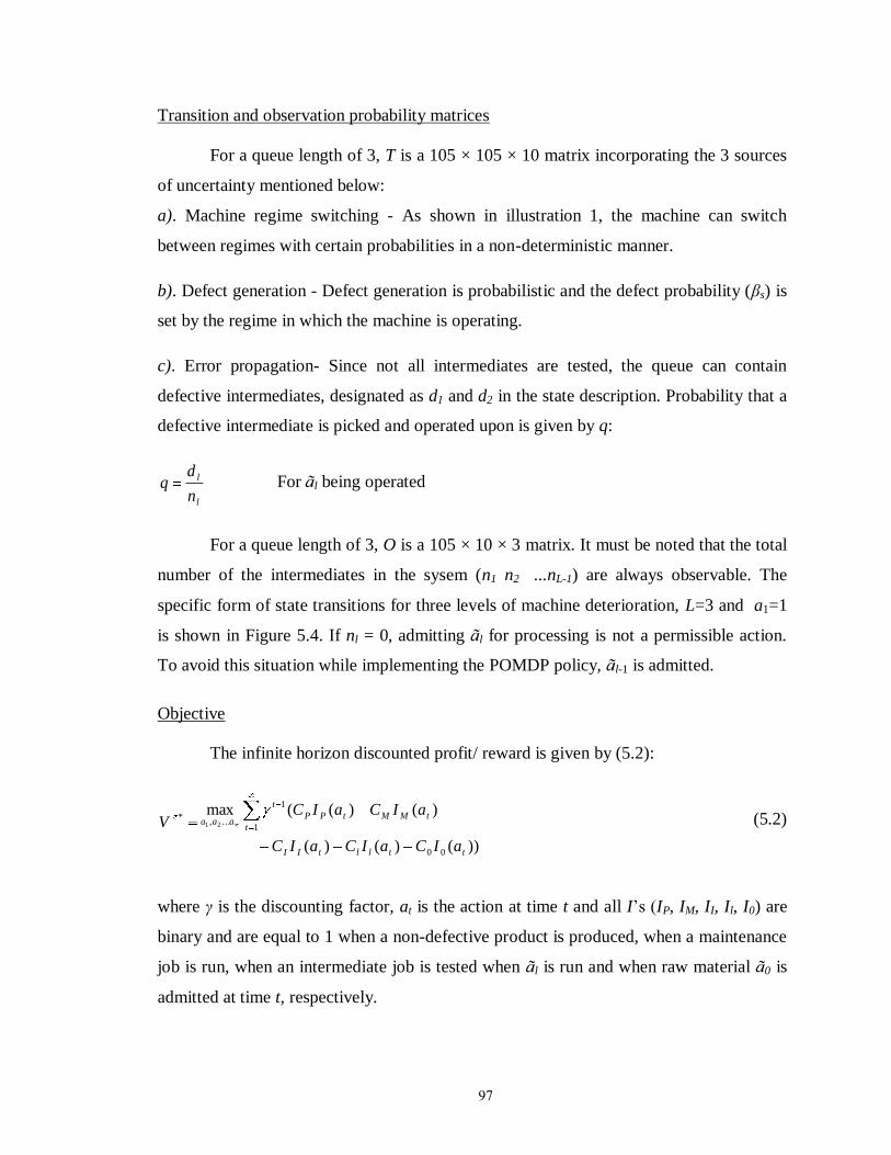
97
Transition and observation probability matrices
For a queue length of 3, T is a 105 × 105 × 10 matrix incorporating the 3 sources
of uncertainty mentioned below:
a). Machine regime switching - As shown in illustration 1, the machine can switch
between regimes with certain probabilities in a non-deterministic manner.
b). Defect generation - Defect generation is probabilistic and the defect probability (βs) is
set by the regime in which the machine is operating.
c). Error propagation- Since not all intermediates are tested, the queue can contain
defective intermediates, designated as d1 and d2 in the state description. Probability that a
defective intermediate is picked and operated upon is given by q:
l
l
n
dq For l being operated
For a queue length of 3, O is a 105 × 10 × 3 matrix. It must be noted that the total
number of the intermediates in the sysem (n1 n2 ...nL-1) are always observable. The
specific form of state transitions for three levels of machine deterioration, L=3 and a1=1
is shown in Figure 5.4. If nl = 0, admitting l for processing is not a permissible action.
To avoid this situation while implementing the POMDP policy, l-1 is admitted.
Objective
The infinite horizon discounted profit/ reward is given by (5.2):
))()()(
)()((max
00
1
1
...,*
21
ttlltII
t
tMMtPP
t
aaa
aICaICaIC
aICaICV
(5.2)
where γ is the discounting factor, at is the action at time t and all I‟s (IP, IM, II, Il, I0) are
binary and are equal to 1 when a non-defective product is produced, when a maintenance
job is run, when an intermediate job is tested when l is run and when raw material 0 is
admitted at time t, respectively.
98
′ =1
renew[n1 n2 d1 d2 ]p 1
p 2
p 3
y
n ′ =2
′ =3
′ =1
′ =1
renew[n1 n2 d1 d2 ]p 1
p 2
p 3
y
n ′ =2
′ =3
′ =1
(a)
(b)
[n1 n2 d1 d2 ′ ]
a0
a1
a2
[n1-1 n2+1 d1 d2 ′]
[n1-1 n2+1 d1 d2+1 ′]
[n1-1 n2+1 d1-1 d2 +1 ′]
[n1-1 n2+1 d1-1 d2+1 ′]
p_1
p_2
p_3
p_4
admit
[n1-1 n2+1 d1 d2 ′]
o=o1
inspect
y
n
[n1-1 n2+1 d1 d2 ′]
o=o3
[n1-1 n2 d1 d2 ′]
o=o2
inspect
y
n
[n1-1 n2+1 d1 d2+1 ′]
o=o3
[n1-1 n2 d1-1 d2 ′]
o=o1
inspect
y
n
[n1-1 n2+1 d1-1 d2+1 ′]
o=o3
[n1-1 n2 d1-1 d2 ′]
o=o2
inspect
y
n
[n1-1 n2+1 d1-1 d2+1 ′]
o=o3
[n1 n2 d1 d2 ′ ]
a0a0
a1a1
a2a2
[n1-1 n2+1 d1 d2 ′]
[n1-1 n2+1 d1 d2+1 ′]
[n1-1 n2+1 d1-1 d2 +1 ′]
[n1-1 n2+1 d1-1 d2+1 ′]
p_1
p_2
p_3
p_4
admit
[n1-1 n2+1 d1 d2 ′]
o=o1
inspect
y
n
inspect
y
n
[n1-1 n2+1 d1 d2 ′]
o=o3
[n1-1 n2 d1 d2 ′]
o=o2
inspect
y
n
inspect
y
n
[n1-1 n2+1 d1 d2+1 ′]
o=o3
[n1-1 n2 d1-1 d2 ′]
o=o1
inspect
y
n
inspect
y
n
[n1-1 n2+1 d1-1 d2+1 ′]
o=o3
[n1-1 n2 d1-1 d2 ′]
o=o2
inspect
y
n
inspect
y
n
[n1-1 n2+1 d1-1 d2+1 ′]
o=o3
(c)
Figure 5.4: State transition for the re-entrant flow problem for 3 levels of machine
deterioration and L=3 (a) Possible values of the machine condition at the next time step
( ′) given the current machine condition ( ) and the renewal decision. (b) Probabilities
associated with defect generation ( ) and propagation ( 11 nd ). (c) Possible next states
and observations depending upon job scheduling and job inspection decisions and
realization of uncertainty.
1
1
1
1
1
1
1
1
4_;)1(3_
);1(2_);1)(1(1_
n
dp
n
dp
n
dp
n
dp
99
The maximum allowable size of the queue largely governs the size of the state
space which eventually controls the size of the problem. The above problem is solved for
maximum queue lengths of 3, 4 and 5. Three different parameter sets (4, 5 and 6) shown
in Table 5.1(a) are considered.
The parameter values are reasonably chosen to represent the trade-offs among
different cost heads in a typical manufacturing environment. Since the queue length is
constrained, holding cost/ work in progress (WIP) cost is not considered. All problem
instances are solved using the algorithm shown in Figure 5.5. An initial belief sample set
is obtained by using three different policies (i) optimal policy for the FOMDP problem,
(ii) best periodic or block replacement and inspection policy, and (iii) policy to select a
random action at each time. The algorithm uses PERSEUS iterations on the fixed initial
belief set until ε convergence is achieved. A new sample is then obtained using the
current value function for POMDP and the above is repeated (this is called one sample
iteration). These sample iterations are carried out until the performance of two
subsequent sample iterations is found to be δ-close for a randomly chosen test belief set.
The results are reported in Table 5.2. Table 5.2 includes the size of the problem
for the queue sizes considered. |V| is the size of the optimal policy, i.e., the number of
gradient vectors i
n , i= 1, 2, .., |Vn|. Profit for POMDP is the average profit obtained by
starting in s=1 ([0 0 0 0 1] -no jobs in the system and best machine condition) and
following the optimal policy. Average is taken over 100 experiments in all cases.
FOMDP profit reported for starting in state s=1, acts as the theoretical upper bound and
cannot be achieved. The difference in the two values provides the extent to which the
partial observability affects the performance. For parameter set 5, the processing costs for
layers 1,2 and 3 are higher as compared to those for parameter set 4. This causes
reduction in the overall profit as compared with parameter set 4 but evidently no
difference in the optimal policy for fully observable problems. However, in the partially
observable case, the (near) optimal policy results in increase in average queue size
(number of intermediates in the queue at any time) with increase in processing cost. This
is because the system is more cautious about running an expensive intermediate when
100
machine deterioration level is high. In parameter set 6, the defect probabilities associated
with machine deterioration levels 2 and 3 are increased, which leads to further reduction
in overall profit. The general characteristics of FOMDP policies are discussed in further
details.
5.3.3 Characterization of FOMDP policy
In order to understand the system behavior, the optimal policy corresponding to
the FOMDP problem is analyzed. It is seen that the machine renewal, job inspection and
job scheduling decisions are mutually correlated and therefore a compact representation
of the policy is not possible. The general characteristics of the optimal policy are
discussed further:
1. The optimal policy is a strong function of the probability of defect generation and
that of defect propagation. The former is the determined by s, the defect
probability associated with machine deterioration level s and the latter is the
probability that the incoming job is already defective. The latter is given by dl/nl.
Also the term „expensive intermediate‟ is used to denote al with relatively large l.
2. The machine is renewed when defect generation probability is high (3 and(or) 2)
and defect propagation probability is low.
3. Job inspection is carried out when both of the above probabilities are high and
when an expensive intermediate is admitted for processing. Note that according to
problem specification, L is always tested.
4. An expensive intermediate l is admitted for processing whenever nl 0 and defect
generation and propagation probabilities are low. Otherwise, al-1 is picked for
processing.
For the cost values considered, the system tends to keep a small number of
intermediates in the system as guided by the optimal policy. This is the reason why the
optimal policy and the performance of the reentrant flow problems with varying limits on
queue sizes (3,4 and 5) are the same (please see Table 5.2). As for the structure of the
POMDP policy, trends similar to the FOMDP policy are observed. However, job
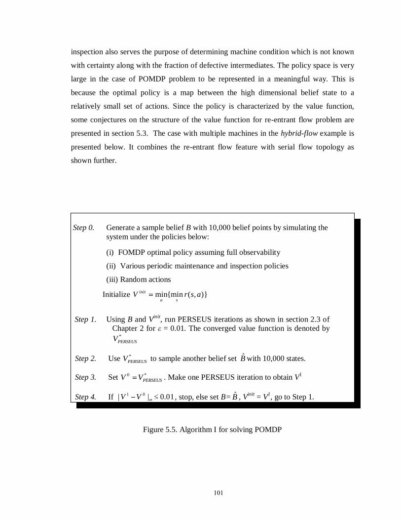
101
inspection also serves the purpose of determining machine condition which is not known
with certainty along with the fraction of defective intermediates. The policy space is very
large in the case of POMDP problem to be represented in a meaningful way. This is
because the optimal policy is a map between the high dimensional belief state to a
relatively small set of actions. Since the policy is characterized by the value function,
some conjectures on the structure of the value function for re-entrant flow problem are
presented in section 5.3. The case with multiple machines in the hybrid-flow example is
presented below. It combines the re-entrant flow feature with serial flow topology as
shown further.
Step 0. Generate a sample belief B with 10,000 belief points by simulating the
system under the policies below:
(i) FOMDP optimal policy assuming full observability
(ii) Various periodic maintenance and inspection policies
(iii) Random actions
Initialize )},(min{min asrVsa
init
Step 1. Using B and Vinit
, run PERSEUS iterations as shown in section 2.3 of
Chapter 2 for ε = 0.01. The converged value function is denoted by *
PERSEUSV
Step 2. Use *
PERSEUSV to sample another belief set B with 10,000 states.
Step 3. Set *0
PERSEUSVV . Make one PERSEUS iteration to obtain V1
Step 4. If 01.0|| 01 VV , stop, else set B= B , Vinit
= V1, go to Step 1.
Figure 5.5. Algorithm I for solving POMDP
102
5.4 A hybrid flow example – modeling and solution
5.4.1 System Description
Illustration 3: There are three machines (A,B,C) similar to the one in Illustration 1
that undergo degradation according to separate independent Markov chains and defect
probabilities. The machines are in series and the jobs have a pre-defined order of
operation as shown below:
1. Three layers at machine
2. Two layers at machine
3. One layer at machine
where layer again refers to one machine operation for simplicity. The jobs being operated
at machines , and are designated as l, l, and l respectively, where the subscript l
refers to the number of layers already deposited. The process is schematically shown in
Figure 5.6. Due to the difference in times of operation, the machines must deteriorate
after each run in this case. However, for simplicity, it is assumed that all machines can
transition to a lower deterioration level at each time unit but the result is only reflected on
the next job to be processed and not the current job. There is an inspection station after
machines and . If an intermediate is tested and found defective, it is sent to a repair
station where only the topmost layer can be repaired. It costs CR for each repair and the
repaired job is returned to the system for further processing. It takes 2 time units for an
operation at , 3 units at and 6 units at . Unlike in Illustration 2, there is no possibility
of queuing the jobs in this system. Jobs are fed sequentially, there is one job at each
machine at any time and product is obtained every 6 time units. It is assumed that
machine maintenance, job inspection and rework take negligible time. However, if a
defect is detected in the last layer of or , then repair is not required and it can be
repaired by the subsequent operation ( or resp.) without any additional cost. Reward
is received only when all the layers in the final product 1 are non-defective. The
objective is to maximize the average infinite horizon discounted profit while obtaining an
optimal renewal policy and job inspection policy for all three operations. It is assumed
that the final product is always tested.
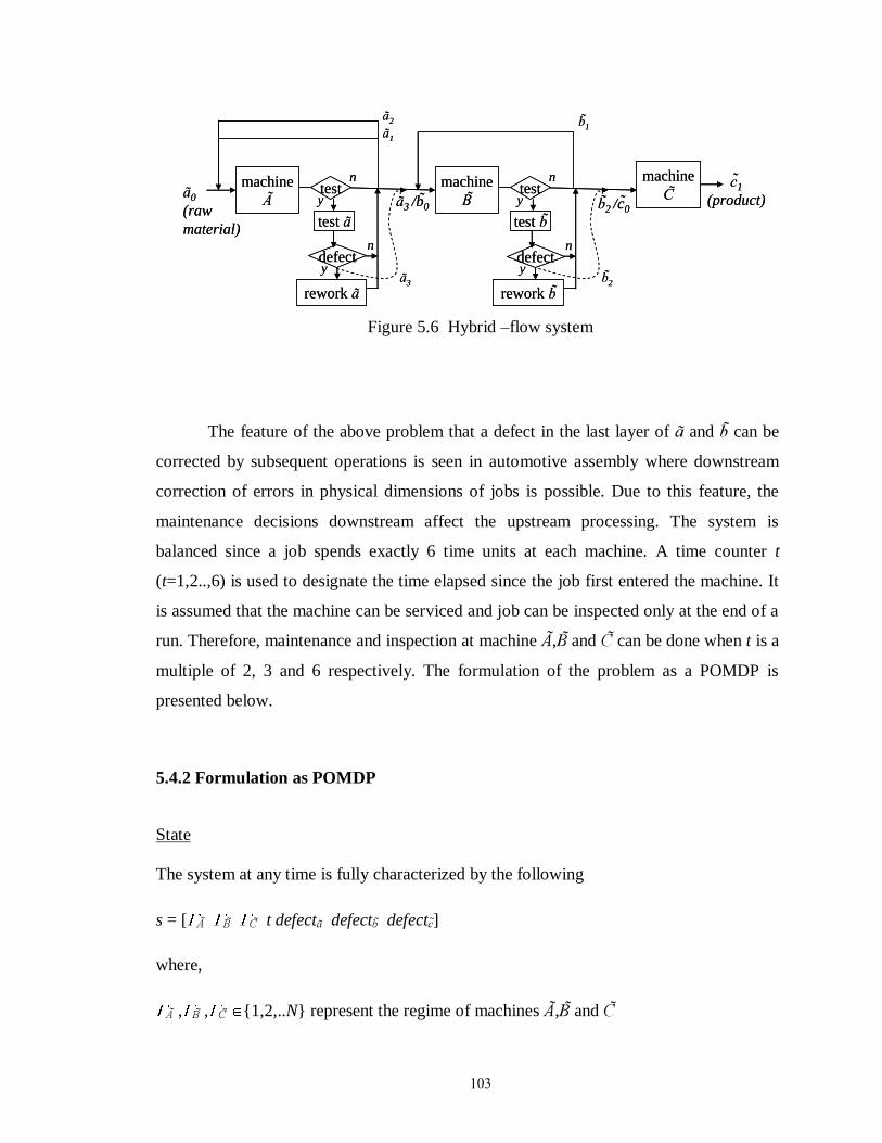
103
machine
A
test a
rework a
c1
(product)
a1
a2
a0
(raw
material)
testy
n machine
B
b1
testy
n
a3 /b 0
machine
C
defecty
n
test b
rework b
defecty
n
b2 /c 0
a3 b2
machine
A
test a
rework a
c1
(product)
a1
a2
a0
(raw
material)
testy
n machine
B
b1
testy
n
a3 /b 0
machine
C
defecty
n
test b
rework b
defecty
n
b2 /c 0
a3 b2
Figure 5.6 Hybrid –flow system
The feature of the above problem that a defect in the last layer of and can be
corrected by subsequent operations is seen in automotive assembly where downstream
correction of errors in physical dimensions of jobs is possible. Due to this feature, the
maintenance decisions downstream affect the upstream processing. The system is
balanced since a job spends exactly 6 time units at each machine. A time counter t
(t=1,2..,6) is used to designate the time elapsed since the job first entered the machine. It
is assumed that the machine can be serviced and job can be inspected only at the end of a
run. Therefore, maintenance and inspection at machine , and can be done when t is a
multiple of 2, 3 and 6 respectively. The formulation of the problem as a POMDP is
presented below.
5.4.2 Formulation as POMDP
State
The system at any time is fully characterized by the following
s = [ t defect defect defect ]
where,
, , {1,2,..N} represent the regime of machines , and
104
t1 {1,2,..,6} time elapsed until the jobs , , started getting processed at machine ,
and respectively.
defect {0,1} shows whether the jobs that are being processed have one or more
defective layer(s) (1) or not (0)
Action/ decision
a = [renew renew renew test test ]
renewi {0,1} for i = , , , pertains to whether to renew the machine i (1) or not (0)
testi {0,1} for i= , pertains to whether to test the processed job i(1) or not (0)
Observation
o = [o o o ]
where oi {o1,o2,o3} for i= ,
oi {o1,o2} for i=
This is because the final product is always tested
Transition Probability Matrix
T incorporates the following sources of uncertainty
a). Machine regime switching - As shown in illustration 1 (Figure 5.4(a)), the machines
can switch between regimes with certain probabilities in a non-deterministic manner.
b). Defect generation - Defect generation is probabilistic and the defect probability (βs) is
set by the regime in which the machines are operating.
Objective
Maximization of the infinite horizon discounted profit/ reward given by (5.3):
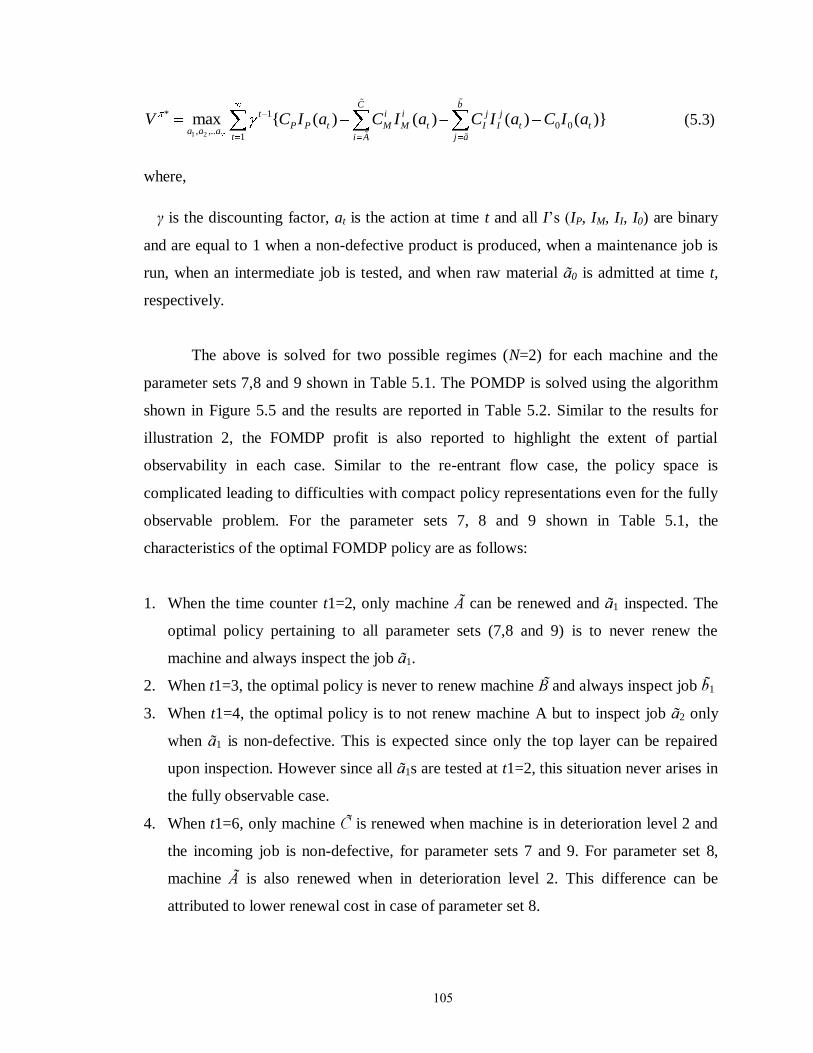
105
1 2
* 1
0 0, ,..
1
max { ( ) ( ) ( ) ( )}C b
t i i j j
P P t M M t I I t ta a a
t j ai A
V C I a C I a C I a C I a
(5.3)
where,
γ is the discounting factor, at is the action at time t and all I‟s (IP, IM, II, I0) are binary
and are equal to 1 when a non-defective product is produced, when a maintenance job is
run, when an intermediate job is tested, and when raw material 0 is admitted at time t,
respectively.
The above is solved for two possible regimes (N=2) for each machine and the
parameter sets 7,8 and 9 shown in Table 5.1. The POMDP is solved using the algorithm
shown in Figure 5.5 and the results are reported in Table 5.2. Similar to the results for
illustration 2, the FOMDP profit is also reported to highlight the extent of partial
observability in each case. Similar to the re-entrant flow case, the policy space is
complicated leading to difficulties with compact policy representations even for the fully
observable problem. For the parameter sets 7, 8 and 9 shown in Table 5.1, the
characteristics of the optimal FOMDP policy are as follows:
1. When the time counter t1=2, only machine can be renewed and 1 inspected. The
optimal policy pertaining to all parameter sets (7,8 and 9) is to never renew the
machine and always inspect the job 1.
2. When t1=3, the optimal policy is never to renew machine and always inspect job 1
3. When t1=4, the optimal policy is to not renew machine A but to inspect job 2 only
when 1 is non-defective. This is expected since only the top layer can be repaired
upon inspection. However since all 1s are tested at t1=2, this situation never arises in
the fully observable case.
4. When t1=6, only machine is renewed when machine is in deterioration level 2 and
the incoming job is non-defective, for parameter sets 7 and 9. For parameter set 8,
machine is also renewed when in deterioration level 2. This difference can be
attributed to lower renewal cost in case of parameter set 8.
106
The high dimensionality associated with the (near) optimal policy for the partially
observed hybrid flow problem prevents a compact representation. Some conjectures on
the POMDP policy together with those on the partially observed reentrant flow problem
are presented in the following section. Alternative policies are also discussed in order to
establish the goodness of the POMDP solution.
5.5 Discussion on results and policy discussion
5.5.1 Performance Comparison
In order to understand the advantages of a rigorous approach to solving this class
of problems, the following is used as a basis of comparison:
(i) FOMDP solution – The performace of the MDP, assuming that the system state is
fully observed, establishes a non-achievable upper bound to the POMDP solution and
the gap between the performances show the extent to which the partial observability
affects the system. It also helps understand the policy structure and the relevant
region of the state space in certain cases. The optimal discounted infinite horizon
reward for starting in s=1 for all illustrations and parameter sets is reported in Table
5.2. For the single machine problem, the changing inspection cost has no effect on the
solution since the state is fully observed and inspection is never carried out. (State
s=1 in all illustrations, represents the starting state with the best machine regime(s)
and no jobs in the system).
(ii) QMDP
approximation – A lower bound on the close-to-optimal solution of the POMDP
is established by using a simple function approximation scheme (Hauskretch 2000).
The optimal Q-function associated with the fully observable MDP is shown in (5.4),
where VMDP
is the optimal value function. The Q-function associated with the
partially observed problem for each belief state and action is then approximated as
shown in (5.5). The resulting performance is contained in Table 5.2. Note that the
optimal policy corresponding to the FOMDP does not contain the inspection decision
for gauging machine regime when states are fully observed. That is the reason why, at
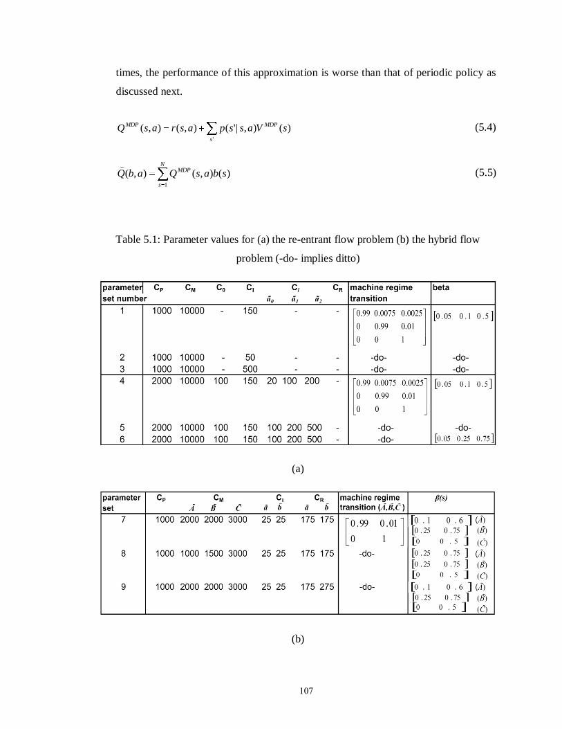
107
times, the performance of this approximation is worse than that of periodic policy as
discussed next.
'
)(),|'(),(),(s
MDPMDP sVasspasrasQ (5.4)
N
s
MDP sbasQabQ1
)(),(),(
(5.5)
Table 5.1: Parameter values for (a) the re-entrant flow problem (b) the hybrid flow
problem (-do- implies ditto)
(a)
(b)
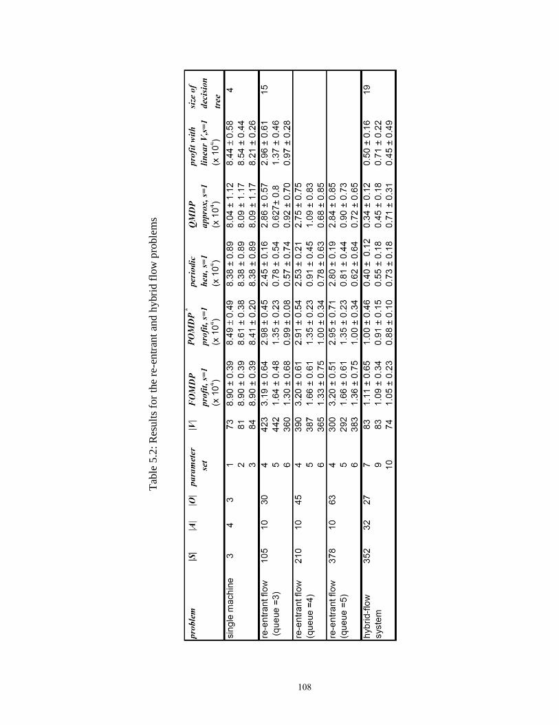
108
Tab
le 5
.2:
Res
ult
s fo
r th
e re
-entr
ant
and h
ybri
d f
low
pro
ble
ms
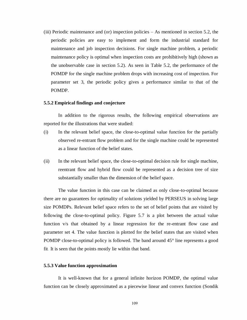
109
(iii) Periodic maintenance and (or) inspection policies – As mentioned in section 5.2, the
periodic policies are easy to implement and form the industrial standard for
maintenance and job inspection decisions. For single machine problem, a periodic
maintenance policy is optimal when inspection costs are prohibitively high (shown as
the unobservable case in section 5.2). As seen in Table 5.2, the performance of the
POMDP for the single machine problem drops with increasing cost of inspection. For
parameter set 3, the periodic policy gives a performance similar to that of the
POMDP.
5.5.2 Empirical findings and conjecture
In addition to the rigorous results, the following empirical observations are
reported for the illustrations that were studied:
(i) In the relevant belief space, the close-to-optimal value function for the partially
observed re-entrant flow problem and for the single machine could be represented
as a linear function of the belief states.
(ii) In the relevant belief space, the close-to-optimal decision rule for single machine,
reentrant flow and hybrid flow could be represented as a decision tree of size
substantially smaller than the dimension of the belief space.
The value function in this case can be claimed as only close-to-optimal because
there are no guarantees for optimality of solutions yielded by PERSEUS in solving large
size POMDPs. Relevant belief space refers to the set of belief points that are visited by
following the close-to-optimal policy. Figure 5.7 is a plot between the actual value
function v/s that obtained by a linear regression for the re-entrant flow case and
parameter set 4. The value function is plotted for the belief states that are visited when
POMDP close-to-optimal policy is followed. The band around 45° line represents a good
fit. It is seen that the points mostly lie within that band.
5.5.3 Value function approximation
It is well-known that for a general infinite horizon POMDP, the optimal value
function can be closely approximated as a piecewise linear and convex function (Sondik
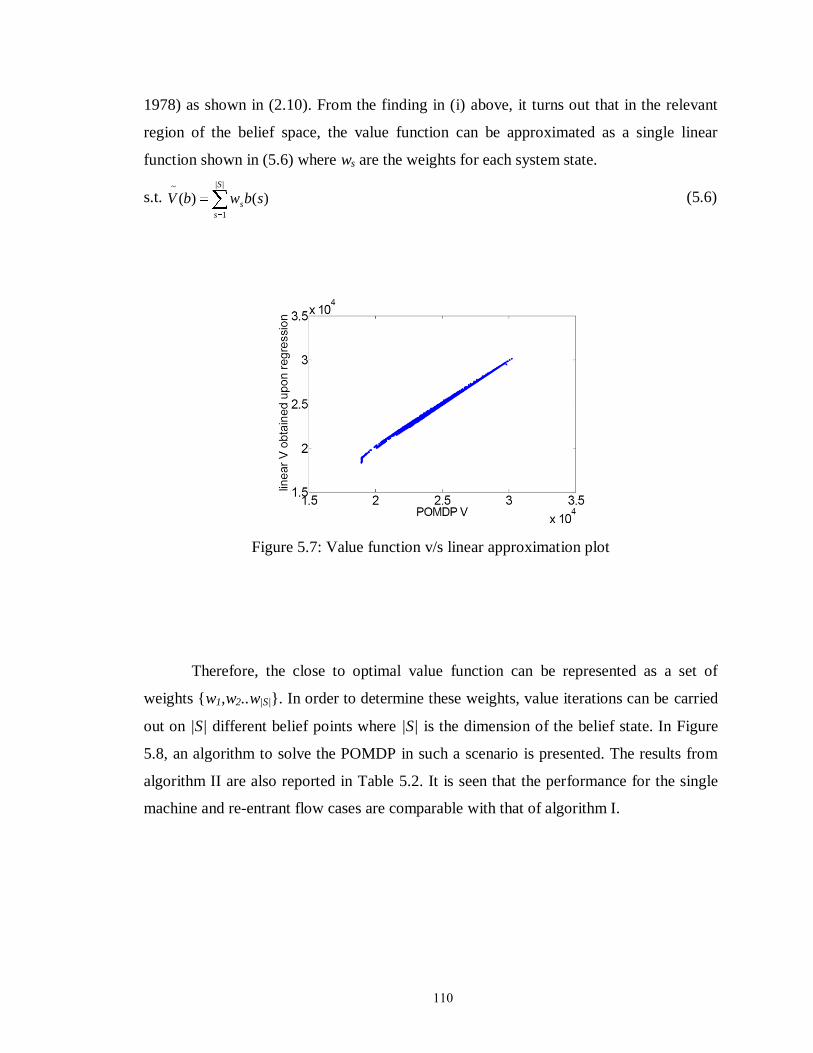
110
1978) as shown in (2.10). From the finding in (i) above, it turns out that in the relevant
region of the belief space, the value function can be approximated as a single linear
function shown in (5.6) where ws are the weights for each system state.
s.t. ||
1
~
)()(S
s
s sbwbV (5.6)
Figure 5.7: Value function v/s linear approximation plot
Therefore, the close to optimal value function can be represented as a set of
weights {w1,w2..w|S|}. In order to determine these weights, value iterations can be carried
out on |S| different belief points where |S| is the dimension of the belief state. In Figure
5.8, an algorithm to solve the POMDP in such a scenario is presented. The results from
algorithm II are also reported in Table 5.2. It is seen that the performance for the single
machine and re-entrant flow cases are comparable with that of algorithm I.
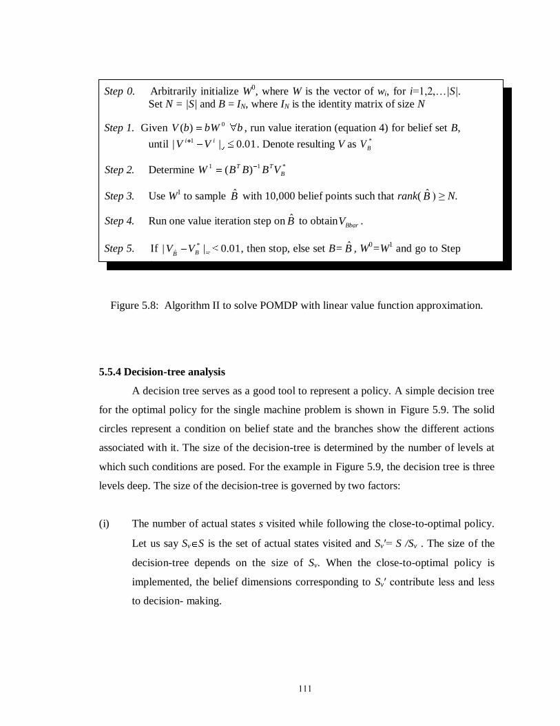
111
Step 0. Arbitrarily initialize W0, where W is the vector of wi, for i=1,2,…|S|.
Set N = |S| and B = IN, where IN is the identity matrix of size N
Step 1. Given bbWbV 0)( , run value iteration (equation 4) for belief set B,
until 01.0|| 1 ii VV . Denote resulting V as *
BV
Step 2. Determine *11 )( B
TT VBBBW
Step 3. Use W1 to sample B with 10,000 belief points such that rank( B ) ≥ N.
Step 4. Run one value iteration step on B to obtainBbarV .
Step 5. If 01.0|| *
ˆ BBVV , then stop, else set B= B , W
0=W
1 and go to Step
1.
Figure 5.8: Algorithm II to solve POMDP with linear value function approximation.
5.5.4 Decision-tree analysis
A decision tree serves as a good tool to represent a policy. A simple decision tree
for the optimal policy for the single machine problem is shown in Figure 5.9. The solid
circles represent a condition on belief state and the branches show the different actions
associated with it. The size of the decision-tree is determined by the number of levels at
which such conditions are posed. For the example in Figure 5.9, the decision tree is three
levels deep. The size of the decision-tree is governed by two factors:
(i) The number of actual states s visited while following the close-to-optimal policy.
Let us say Sv S is the set of actual states visited and Sv′= S /Sv . The size of the
decision-tree depends on the size of Sv. When the close-to-optimal policy is
implemented, the belief dimensions corresponding to Sv′ contribute less and less
to decision- making.
112
Figure 5.9: Decision tree for the single machine problem. Values of 1,2 and 3 for a
represent the decisions to „do nothing‟ , „inspect the job‟ and „service the equipment‟
respectively.
(ii) The level of similarity between actual states s – due to the similarity, a cluster of
states would correspond to the same (near)optimal action. In the region of belief
states, the states belonging to these clusters would form hyper-planes and lead to a
decision-tree of much lower dimension. The sizes of the decision-trees are also
reported in Table 5.2 and are substantially smaller than the size of Sv. This
indicates the formation of clusters of states that behave in a similar manner.
5.6 Conclusions
Judging by the research efforts in the area of partially observed degradation of
manufacturing equipment and costly inspection, the extension of the concepts to multiple
operations is important. In this work this problem is addressed for a re-entrant and a
hybrid flow topology. The significance of rigorous treatment of this class of problems is
illustrated by comparing the results with those of heuristic methods. The POMDP
formulations result in significant improvements in performance over those of best
heuristics. However, the POMDP problem grows fast with increasing problem sizes.
Therefore, characterization of the (near) optimal policies is an important direction for
future work in this area.
b(3)<0.9
b(3)<0.76
b(1)<0.1 a=1
a=2
a=3 a=2
113
CHAPTER 6
MILP BASED VALUE BACKUPS IN POMDPS WITH VERY LARGE
OR CONTINUOUS ACTION SPACES
6.1 Introduction
In the last chapter we saw that POMDPs serve as powerful tools to model
stochastic systems with partial state information. Since the exact solution methods for
POMDPs are limited to problems with very small sizes of state, action and observation
spaces, approximate solution methods have gained popularity. Notable among these are
the point based methods which consider a fixed or evolving set of prototype belief points
instead of considering the entire belief simplex. A particular point based method,
PERSEUS (Spaan and Vlassis, 2005) was used in chapter owing to the fact that it
favorably makes use of the piecewise linear and convex (PWLC) structure of the value
function to speed up convergence. In this chapter, we consider POMDPs with very large
or continuous action space. In the current form of PERSEUS and many other point based
methods, presence of continuous actions or very large action space makes it practically
impossible to compute the value backup exactly. We use a mathematical program to
circumvent this difficulty. In an alternative formulation, we develop value iteration
update equations around post decision belief state as opposed to the traditionally used
notion of (pre-decision) belief state. Depending on the size of the observation space,
latter approach reduces the computational load of the mathematical program based value
backup calculation. The requirements on the structure of the reward function and the
dependence of probabilities of state transition and observation on action are provided.
Two illustrations, one each for pre-decision and post-decision belief states are included to
analyze the efficacy of the method. Comparison with enumeration and action sampling
methods is provided in terms of solution quality and solution time.
114
6.2 Related work
Adopting the POMDP notation from Chapters 2 and 5, the value backup for a
belief point b for (infinite horizon POMDP with discount factor γ) is given by (6.1),
where ||,..2,1 n
i
n Vi is the set of gradient vectors that characterizes the value function
at nth iteration. We use infinite horizon POMDP with discounting in all illustrations.
Equivalent models can be derived for finite horizon POMDPs with little difficulty.
})(),|()(),({max)( ,
1
Oo
oa
n
SsAa
n bVabopsbasrbV (6.1)
)(),'|(),|'(
)(),'|(),|'(
)'(
'
,
sbasopassp
sbasopassp
sb
Ss Ss
Ssoa (6.2)
)(),'|(),|'(),|('
sbasopasspabopSs Ss
(6.3)
Ss
oai
ni
oa
n sbsbV'
,, )'()'(max)( (6.4)
As with fully observable Markov decision processes (FO-MDP or simply MDP),
the presence of large and continuous action spaces poses a challenge in terms of
computation of maximization over the entire action space (6.1). Additionally, in case of
the exact solution methods for POMDPs, the size of action space, i.e. |A| also affects the
number of potential gradient vectors which may comprise the value function at the next
iteration. The two aspects are summarized below:
(i) In each value iteration step and in the policy evaluation step of policy iteration
algorithm, the maximization is performed over the entire action space for all or a
subset of prototype belief points. Therefore, for every iteration, the computation time
is proportional to |A| when enumeration of all actions is used.
(ii) For exact solution methods reported by Monahan (1982); Hauskretch (2000), in order
to obtain the value function estimate during nth
iteration, a set of all possible gradient
115
vectors is generated. Linear Programming (LP) is then used to determine the useful
among these vectors. The term useful denotes the gradient vector that maximizes the
value of at least one point in the belief simplex as compared with all other gradient
vectors. The size of all possible gradient vectors at the nth iteration is |Vn||A||O|, where
|Vn| is the number of gradient vectors that characterize Vn.
It is not surprising then that, to the best of our knowledge, no current solution
method claims to compute the max operation exactly for very large or continuous action
spaces. A subset of literature that considers POMDPs with very large or continuous
action spaces is reviewed below.
Policy search methods can handle continuous action spaces. An example is
Pegasus (Ng and Jordan, 2000), which estimates the value of a policy by simulating
trajectories from the POMDP using a fixed random seed, and adapts its policy in order to
maximize this value. Pegasus can handle continuous action spaces at the cost of a sample
complexity that is polynomial in the size of the state space. Baxter and Bartlett (2001)
propose a policy gradient method that searches in the space of randomized policies, and
which can also handle continuous actions. The main disadvantages of policy search
methods are the need to choose a particular policy class and the fact that they are prone to
local optima. Thrun (2000) and Spaan and Vlassis, (2005) consider sampling techniques
to keep the active size of the action space relatively small for continuous or very large
action spaces. The method is problem dependent and may lead to loss of solution quality
in certain applications.
In the Monte Carlo POMDP (MC-POMDP) method of Thrun (2000), real-time
dynamic programming is applied on a POMDP with a continuous state and action space.
In that work, beliefs are represented by sets of samples drawn from the state space, while
Q(b,a) values are approximated by nearest-neighbor interpolation from a (growing) set of
prototype values and are updated by online exploration and the use of sampling-based
Bellman backups. In contrast with PERSEUS, the MC-POMDP method does not exploit
the piecewise linearity and convexity of the value function.
116
6.3 Mathematical programming based value updates
6.3.1 Formulation of the mathematical program
The biggest motivation for using a mathematical program to compute the value
backup for a belief point b is the fact that the value function for infinite horizon POMDP
can be approximated well by a PWLC function (Sondik 1978). The value backup
equation is shown in (6.1). Assuming that the state and observation spaces are finite and
with a little abuse of notation, the reward function ra(s) =r(s,a), state transition
probability function ta(s,s′) = T(a,s,s′) and observation probability function
opa(s′,o)=OP(s′,o) are dependent on action a as shown in (6.5) through (6.7). Here
subscript a suggests dependence on action a; s,s′ and o represent the indices of current
state, next state and observation respectively.
)7.6(,')(),'(
)6.6(',)()',(
)5.6()()(
3
2
1
osafosop
ssafsst
safsr
a
a
a
The equivalent mathematical program for (6.1) can be written as shown in (6.8)
through (6.13). )'()',( ssi i
nn is used for ease of notation.
..
})()(),'()',()()({max'
ts
ovsbosopsstsbsrOo
a
Ss Ss
a
Ss
aAa (6.8)
osbsiovSs
oa
ni
'
, )'()',(max)( (6.9)
')(),'()',(
)(),'()',(
)'(
'
, ssbosopsst
sbosopsst
sba
Ss Ss
a
a
Ss
a
oa (6.10)
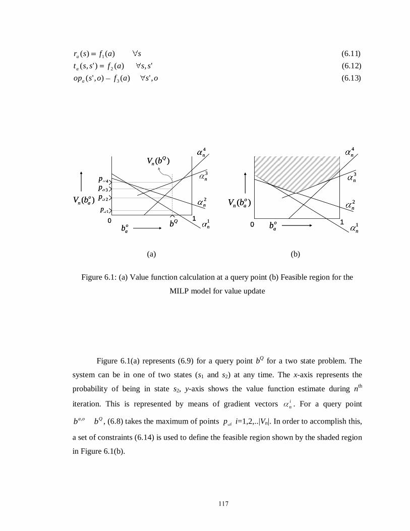
117
)13.6(,')(),'(
)12.6(',)()',(
)11.6()()(
3
2
1
osafosop
ssafsst
safsr
a
a
a
0 1o
ab
)( o
an bV
1
n
2
n
3
n
4
n
Qb
2p
1p
3p4p
)( Q
n bV
0 1o
ab
)( o
an bV
1
n
2
n
3
n
4
n
Qb
2p
1p
3p4p
)( Q
n bV
0 1o
ab
)( o
an bV
1
n
2
n
3
n
4
n
0 1o
ab
)( o
an bV
1
n
2
n
3
n
4
n
(a) (b)
Figure 6.1: (a) Value function calculation at a query point (b) Feasible region for the
MILP model for value update
Figure 6.1(a) represents (6.9) for a query point bQ for a two state problem. The
system can be in one of two states (s1 and s2) at any time. The x-axis represents the
probability of being in state s2, y-axis shows the value function estimate during nth
iteration. This is represented by means of gradient vectors i
n . For a query point
Qoa bb , , (6.8) takes the maximum of points ip i=1,2,..|Vn|. In order to accomplish this,
a set of constraints (6.14) is used to define the feasible region shown by the shaded region
in Figure 6.1(b).
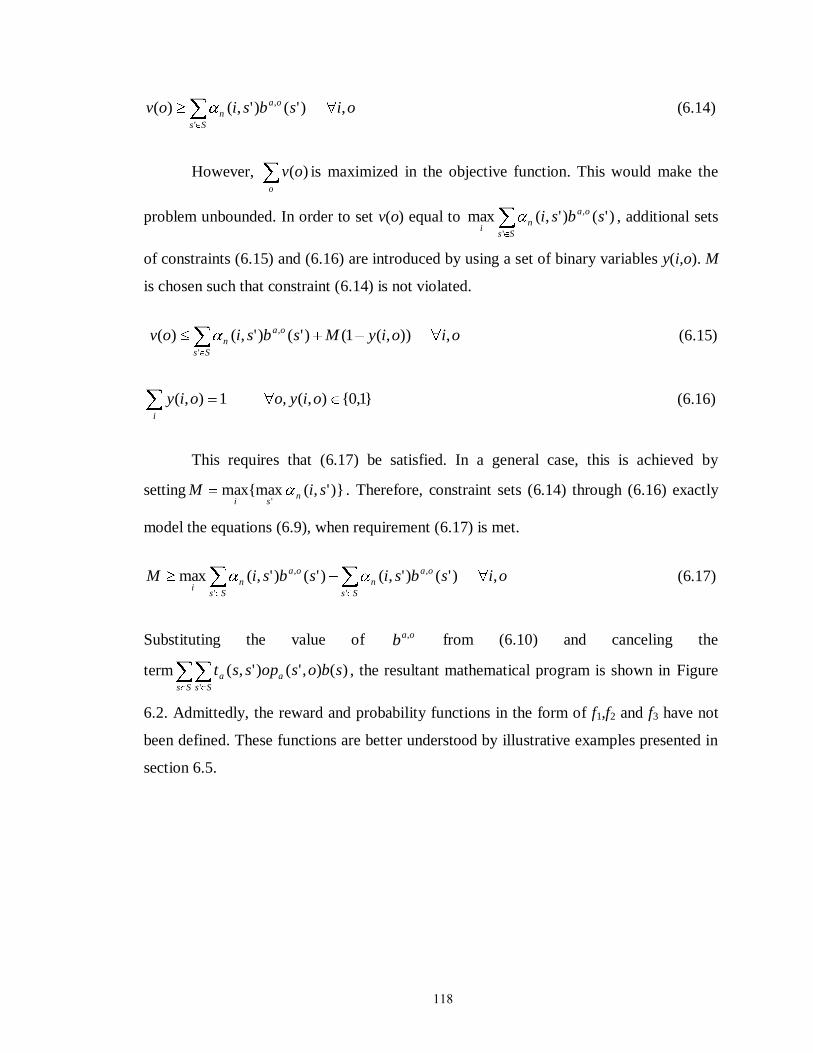
118
oisbsiovSs
oa
n ,)'()',()('
, (6.14)
However, o
ov )( is maximized in the objective function. This would make the
problem unbounded. In order to set v(o) equal to Ss
oa
ni
sbsi'
, )'()',(max , additional sets
of constraints (6.15) and (6.16) are introduced by using a set of binary variables y(i,o). M
is chosen such that constraint (6.14) is not violated.
oioiyMsbsiovSs
oa
n ,)),(1()'()',()('
, (6.15)
}1,0{),(,1),( oiyooiyi
(6.16)
This requires that (6.17) be satisfied. In a general case, this is achieved by
setting )}',(max{max'
siM nsi
. Therefore, constraint sets (6.14) through (6.16) exactly
model the equations (6.9), when requirement (6.17) is met.
oisbsisbsiMSs
oa
n
Ss
oa
ni
,)'()',()'()',(max'
,
'
, (6.17)
Substituting the value of oab , from (6.10) and canceling the
term )(),'()',('
sbosopsst a
Ss Ss
a , the resultant mathematical program is shown in Figure
6.2. Admittedly, the reward and probability functions in the form of f1,f2 and f3 have not
been defined. These functions are better understood by illustrative examples presented in
section 6.5.
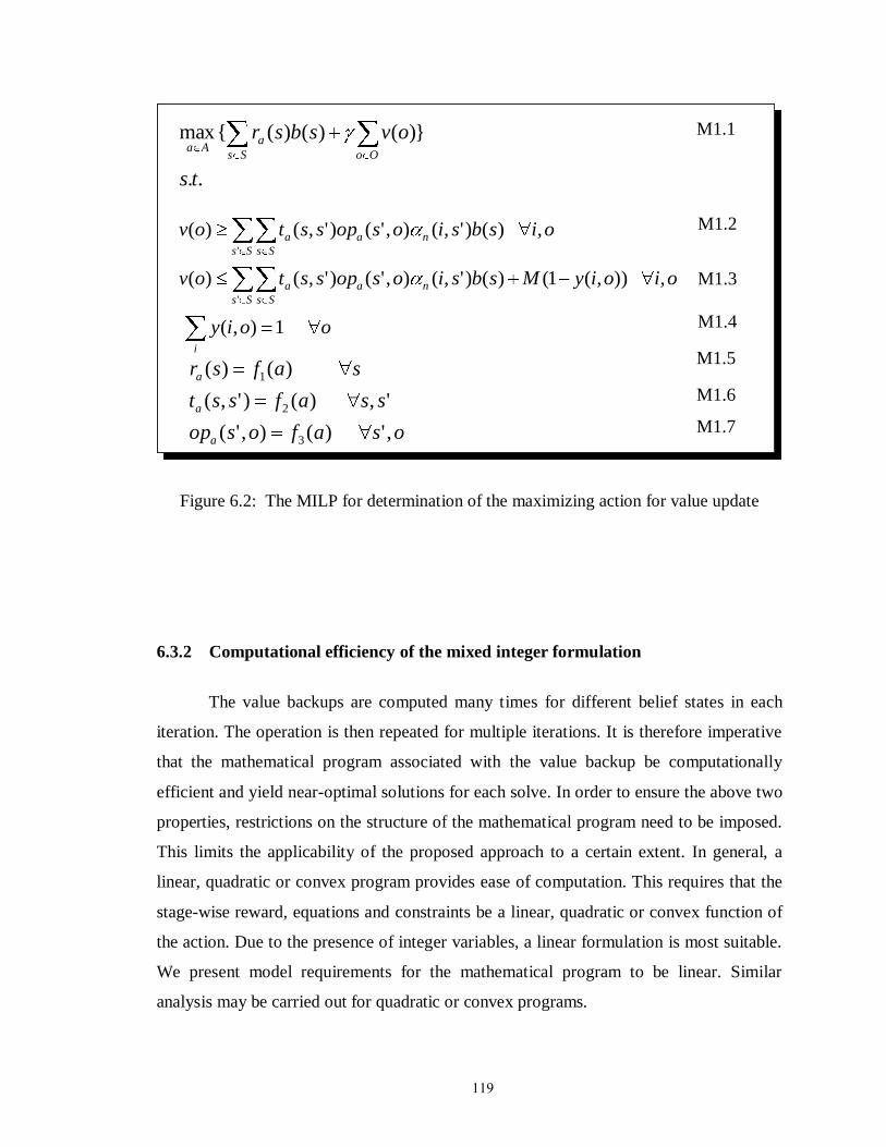
119
..
})()()({max
ts
ovsbsrOoSs
aAa
oisbsiosopsstovSs
na
Ss
a ,)()',(),'()',()('
osafosop
ssafsst
safsr
a
a
a
,')(),'(
',)()',(
)()(
3
2
1
oioiyMsbsiosopsstovSs
na
Ss
a ,)),(1()()',(),'()',()('
ooiyi
1),(
M1.1
M1.2
M1.3
M1.4
M1.5
M1.6
M1.7
..
})()()({max
ts
ovsbsrOoSs
aAa
oisbsiosopsstovSs
na
Ss
a ,)()',(),'()',()('
osafosop
ssafsst
safsr
a
a
a
,')(),'(
',)()',(
)()(
3
2
1
oioiyMsbsiosopsstovSs
na
Ss
a ,)),(1()()',(),'()',()('
ooiyi
1),(
M1.1
M1.2
M1.3
M1.4
M1.5
M1.6
M1.7
Figure 6.2: The MILP for determination of the maximizing action for value update
6.3.2 Computational efficiency of the mixed integer formulation
The value backups are computed many times for different belief states in each
iteration. The operation is then repeated for multiple iterations. It is therefore imperative
that the mathematical program associated with the value backup be computationally
efficient and yield near-optimal solutions for each solve. In order to ensure the above two
properties, restrictions on the structure of the mathematical program need to be imposed.
This limits the applicability of the proposed approach to a certain extent. In general, a
linear, quadratic or convex program provides ease of computation. This requires that the
stage-wise reward, equations and constraints be a linear, quadratic or convex function of
the action. Due to the presence of integer variables, a linear formulation is most suitable.
We present model requirements for the mathematical program to be linear. Similar
analysis may be carried out for quadratic or convex programs.
120
We first list the requirements on reward and probability functions for the model to
be linear and then provide ways to work around some of the requirements. It must be
noted that linearity of the mathematical program is required to assure (near) optimality of
the value backups and to keep the computational load to reasonable limits.
It is easy to see that linearity of the model is determined by the structure of
functions f1,f2 and f3. Due to equations M1.5 through M1.7, the following restrictions are
placed:
(i) f1 is a linear function of action a
(ii) f2 f3 is a linear function of a
Condition (ii) essentially implies that at least one of the functions (f2 and f3) may
not depend on a. This is imposed by constraints M1.2 and M1.3.
Additionally, when functions f1,f2 or f3 involve use of binary variables to represent
logical constraints, the linearity of the model may be affected. Finally, when the system
state has multiple dimensions, it may be necessary to include the entire state description
as opposed to the state indices s and s′ in order to determine stage-wise reward and
probabilities. This aspect is covered in illustration 2.
Whereas condition (i) is true of many real world systems, at the first glance,
condition (ii) appears to be overly restrictive to warrant successful application of the
method. However, a closer look reveals that many real world systems may be modeled
while satisfying condition (ii). It is generally seen that state transition probabilities
depend strongly on action choice, i.e. f2 is a function of a. Observation probabilities (if at
all) depend on discrete actions like whether a sensor measurement is taken. Alternatively,
the discrete decisions that affect observation probabilities may include which or how
many sensors are used for measurement/taking the observation. These discrete decisions
can be made a part of state description leading to observation probabilities depending
only on state s′ and observation o, but independent of action a.
121
6.3.3 Implementation and policy determination
POMDP solution algorithm
The mathematical program shown in Figure 6.2 is a general model to determine
value backup for a belief point b when the parameterized form of value function is used.
PERSEUS, described in Chapter 2 and used for solving the POMDPs in Chapter 5 is one
such algorithm. It directly uses the parametric form of the value function by maintaining
a finite set of gradient vectors αn. Gradient updates are obtained together with value
updates around a prototype belief set, B, as outlined in section 2.3 of Chapter 2. The
updated vector }{
1
b
n is admitted in Vn+1 only if it improves the value at point b as
compared with Vn. Otherwise, }{b
n is admitted. When value backups are obtained using
MILP, the gradient can be easily calculated using the maximizing action a*{b}
. It is also
possible to obtain the gradient vector directly from the MILP solve (but this is not
considered here).
Policy determination
Having obtained the estimate of optimal value function that satisfies a desired
convergence criterion ε, the ε-optimal policy can be obtained using one of the following
methods
(i) Maximizing action associated with each gradient vector – During a value backup for
belief point b, a gradient vector }{
1
b
n is obtained which has a maximizing action a*{b}
(6.18) associated with it. The corresponding maximizing vectors can be cached with
each gradient vector. The ε-optimal policy πε(b) for belief point b is then given by
(6.19)
s
i
Vi
b ssba )()(maxarg||
}*{ (6.18)
}*{)( bab (6.19)
122
However, it may be expensive to hold the entire action descriptions, for each gradient
vector, when the dimension of actions is large.
(ii) One step look ahead controller – The ε-optimal policy πεLA
(b) for a belief point b can
also be obtained in real time by running the value backup operation at each time. This
is shown in (6.20), together with (6.2) , (6.3) and (6.4).
})(),|()()({maxarg)( ,
Oo
oa
Ss
aAa
LA bVabopsbsrb (6.20)
Generally speaking, the first approach is computationally more favorable but may
have high memory requirements if the dimension of the actions is large. It can be shown
that policy LA is at least as good as in an average sense.
6.3.4 Problem size v/s computational complexity
As seen from the model in Figure 6.2, the size of the model (number of variables
and constraints) is directly proportional to |S|2, |O| and |Vn|. Dependence of |A| is implicit.
Since f1, f2 and f3 are transition functions, in the absence of logical variables they pose
little computational challenge. The size of the model is greatly affected by the number of
integer variables i.e., y(i,o) in this case. This number clearly depends on |Vn| and |O|.
While |O| comes directly from the model, the size of Vn is governed by a combination of
factors. The most important factor is the dimensionality of belief simplex. In terms of
PERSEUS, a higher dimensional simplex would require higher number of belief points
comprising the prototype belief set and |Vn| ≤ |B|. However, in practice |Vn| <<|B| (Spaan
and Vlassis, 2005). Another determinant of |Vn| is the structure of optimal policy. E.g.,
when the decision region is convex, it is possible to approximate the function
corresponding to each decision region by very few gradient vectors. In this case, |Vn|
would depend on |A|. In general however, it is difficult to predict the size of Vn from the
model. When |Vn| is very large, we propose some heuristics to pick from the existing
(potentially large) set of gradient vectors, the set which has the most potential for
representing the entire value function. The idea is to construct an active set of gradient
123
vectors Vn_active to feed into the MILP during each iteration. The size of the active set
cannot exceed a pre-defined limit δ, which is chosen to keep the computation time for
each backup within prescribed limits.
(i) Top pick approach – In this approach, the gradient vectors belonging to Vn are
arranged in decreasing order of the total number of belief points that they maximize.
When |Vn|>δ, the top fraction εδ are made a part of the action set Vn_active. In order to
avoid local optima, the remaining fraction (1-ε)δ is chosen randomly from Vn. The
parameter ε represents the classic trade-off between exploration and exploitation
during optimization. Starting with a value close to 0.5, ε may be increased gradually
with the iteration count n.
(ii) Nearest neighbor approach – This approach is based on the fact that certain gradient
vectors may only marginally improve the value at a belief point over some other
vector. For each belief state, it is possible to obtain the gradient that maximizes the
value at the point and also the gradient that gives the next best value. From the set of
maximizing gradient and the next best gradient for each belief point, it is possible to
obtain a set of gradient vectors whose maximum size |B|/2.
The gradient sampling technique is similar in spirit with action sampling methods.
While the size of action space grows exponentially with the dimension of action, |Vn|
generally grows exponentially with |S|. Efficiency of either methods (enumeration or
MILP based value backups) would be determined by the particular application.
While the above approaches to limit the size of Vn appear rather brute force, there
is a more elegant way to resolve the problem of large sized observation spaces. This is
addressed in the following section.
6.4 Value iteration around post decision belief state
6.4.1 The basic idea
For a general MDP (fully observable), the notion of post decision state applies to
problems where the effect of actions and uncertainty on state variable can be separately
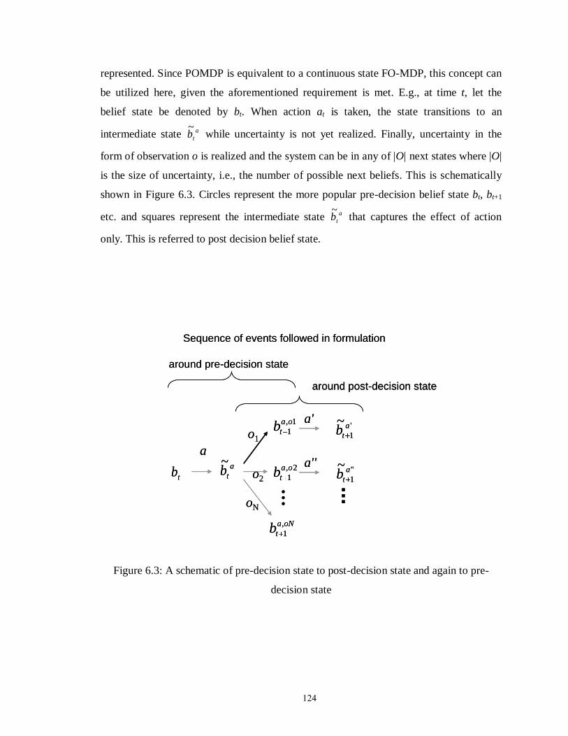
124
represented. Since POMDP is equivalent to a continuous state FO-MDP, this concept can
be utilized here, given the aforementioned requirement is met. E.g., at time t, let the
belief state be denoted by bt. When action at is taken, the state transitions to an
intermediate state a
tb~
while uncertainty is not yet realized. Finally, uncertainty in the
form of observation o is realized and the system can be in any of |O| next states where |O|
is the size of uncertainty, i.e., the number of possible next beliefs. This is schematically
shown in Figure 6.3. Circles represent the more popular pre-decision belief state bt, bt+1
etc. and squares represent the intermediate state a
tb~
that captures the effect of action
only. This is referred to post decision belief state.
a
tb~
tb
a
o1
oN
o2
1,
1
oa
tb
2,
1
oa
tb
oNa
tb ,
1
'
1
~a
tba'
''
1
~a
tba''
Sequence of events followed in formulation
around post-decision state
around pre-decision state
a
tb~
tb
a
o1
oN
o2
1,
1
oa
tb
2,
1
oa
tb
oNa
tb ,
1
'
1
~a
tba'
''
1
~a
tba''
Sequence of events followed in formulation
around post-decision state
around pre-decision state
Figure 6.3: A schematic of pre-decision state to post-decision state and again to pre-
decision state

125
In the context of POMDPs, solution using this approach is possible when the
observation probabilities do not depend on action a. As pointed out in section 6.3.2, the
actions that affect observation probabilities may be made part of the state. The transition
from regular belief state bt to a
tb~
then is simply given by tabt.
It is to be noted that although the effect of action on underlying states s S may be
prone to uncertainty, the belief state transition (tabt) is always deterministic. Having
obtained the post decision belief state, |O| (pre-decision) belief states may be obtained at
the next time step. The transition is governed by the observation probabilities
p(o|bt)=p(o| a
tb~
) for all o O. This two step transition is shown in Figure 6.3. Intuitively,
starting with a post decision state a, |O| possible next states ob oa, are obtained. For
each of the states ob oa, , a maximizing action a′ *{o}
would determine the next post
decision belief state ba′,o
. Consequently, the value iteration update takes the form shown
in (6.22) through (6.26). Va represents value function around post-decision belief state
a.
For notational ease, the dependence of action a′ and next post-decision belief state a′ on
o is suppressed in future illustrations. The details on the derivation of value iteration
equation around post-decision state can be found in (Powell 2007) for a general MDP.
In (6.22), it is to be noted that the expectation over observations is outside the
max operator. This removes the dependence of the size of the MILP on |O|. However, it
still remains to be shown that the structure of Va is PWLC. To this end we first show that
o
aopreaa bVabopbV )(),~
|()~
( (6.21)
and then use Lemma 1 to show that a positive weighted sum of convex functions is
convex. Since 0)~
|( abop , the result holds.
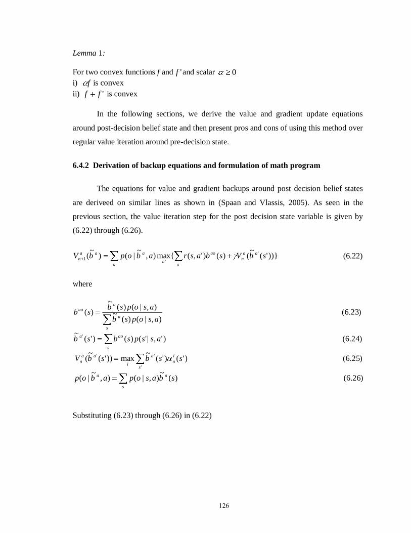
126
Lemma 1:
For two convex functions f and 'f and scalar 0
i) f is convex
ii) 'ff is convex
In the following sections, we derive the value and gradient update equations
around post-decision belief state and then present pros and cons of using this method over
regular value iteration around pre-decision state.
6.4.2 Derivation of backup equations and formulation of math program
The equations for value and gradient backups around post decision belief states
are deriveed on similar lines as shown in (Spaan and Vlassis, 2005). As seen in the
previous section, the value iteration step for the post decision state variable is given by
(6.22) through (6.26).
))}'(~
()()',({max),~
|()~
( '
'1 sbVsbasrabopbV aa
n
ao
sa
o
aaa
n (6.22)
where
s
aa
i
n
s
a
i
aa
n
s
aoa
s
a
aao
sbasopabop
ssbsbV
asspsbsb
asopsb
asopsbsb
)26.6()(~
),|(),~
|(
)25.6()'()'(~
max))'(~
(
)24.6()',|'()()'(~
)23.6(),|()(
~),|()(
~
)(
'
''
'
Substituting (6.23) through (6.26) in (6.22)
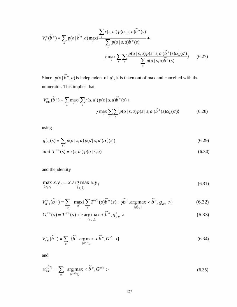
127
)27.6(})(
~),|(
)'()(~
)',|'(),|(max
)(~
),|(
)(~
),|()',(
{max),~
|()~
(
'
'
s s
s
a
i
n
a
i
s
a
a
s
ao
aaa
n
sbasop
ssbasspasop
sbasop
sbasopasr
abopbV
Since ),~
|( abop a is independent of 'a , it is taken out of max and cancelled with the
numerator. This implies that
)28.6(})'()(
~)',|'(),|(max
)(~
),|()',({max)~
(
'
'1
s s
i
n
a
i
a
soa
aa
n
ssbasspasop
sbasopasrbV
using
)30.6(),|()',()(
)29.6()'()',|'(),|()(
'
'
'
asopasrsTand
sasspasopsg
oa
s
i
n
i
oa
and the identity
jy
jy
yxxyxjj
jj
.maxarg..max}{}{
(6.31)
)32.6(},~
maxarg.~
)(~
)({max)~
( '}{
'
'1
'
i
oa
a
g
a
s
aoa
ao
aa
n gbbsbsTbVi
ioa
)33.6(,~
maxarg)()( '}{
''
'
i
oa
a
g
oaoa gbsTsGi
ioa
)34.6(},~
maxarg.~
{)~
( '
}{1
''
oaa
G
a
o
aa
n GbbbVa
oa
and
oaa
Go
b
n Gba
oa
a '
}{
}~
{
1 ,~
maxarg'
'
(6.35)
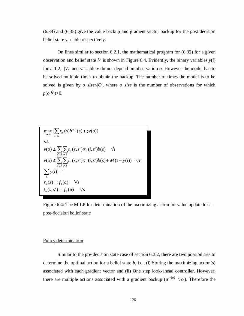
128
(6.34) and (6.35) give the value backup and gradient vector backup for the post decision
belief state variable respectively.
On lines similar to section 6.2.1, the mathematical program for (6.32) for a given
observation and belief state a is shown in Figure 6.4. Evidently, the binary variables y(i)
for i=1,2,. |Vn| and variable v do not depend on observation o. However the model has to
be solved multiple times to obtain the backup. The number of times the model is to be
solved is given by o_size≤|O|, where o_size is the number of observations for which
p(o|a)>0.
safsst
safsr
iy
iiyMsbsisstov
isbsisstov
ts
ovsbsr
a
a
i
Ss Ss
na
Ss Ss
na
Ss
oa
aAa
)()',(
)()(
1)(
))(1()()',()',()(
)()',()',()(
..
)}()()({max
2
1
'
'
,
'
Figure 6.4: The MILP for determination of the maximizing action for value update for a
post-decision belief state
Policy determination
Similar to the pre-decision state case of section 6.3.2, there are two possibilities to
determine the optimal action for a belief state b, i.e., (i) Storing the maximizing action(s)
associated with each gradient vector and (ii) One step look-ahead controller. However,
there are multiple actions associated with a gradient backup (a′*{o}
o ). Therefore the

129
action associated with each observation needs to be cached. This results in higher
memory requirement for storing the ε-optimal policy for the post-decision state, as
compared to that for the pre-decision state. For the look-ahead design on the other hand,
the MILP needs to be solved for the belief state pertaining to the current observation
only. This is computationally less expensive than the look-ahead design for solution
around pre-decision belief state.
6.4.3 Comparison with value updates around pre-decision belief states
While using MILP based value updates the two methods can be compared along
following avenues:
i) Complexity of MILP problem – While using the post formulation several smaller
MILPs are solved for one value backup as opposed to solving one large MILP for
pre-formulation. The former almost always works better if the input/output operations
between the MILP solver (e.g. CPLEX) and regular solution platform (e.g.
MATLAB) are not as time consuming as the optimization itself.
ii) Policy determination in real time – As discussed in the previous section and section
6.3.3, the formulation around pre-decision state allows for storing optimal action with
each gradient vector that characterizes the ε-optimal value function. For formulation
around post-decision belief state optimal action needs to be stored for each gradient
vector and each observation. This increases the memory requirement for the latter.
This may not be feasible in the post formulation when the observation space is very
high. However, the look-ahead design for policy determination is faster for the post-
formulation due to lower complexity of the associated MILP. Consequently, policy
determination in real time in post-formulation can be prohibitively slower.
iii) Handling very large or continuous observation spaces – While pre-formulation is
limited to small observation spaces, the MILP technique for value updates based on
post-formulation is on par with enumeration based methods. When observation space
is very large or continuous, Hoey and Poupart (2005) consider creating sets of
130
observations for which b leads to the same future belief state oab , . This effectively
makes the observation space discrete. Such manipulation of observation probabilities
is better achieved outside the confines of a mathematical program.
Aside from (ii) above, it is easy to see that the two formulations are similar in
terms of computational complexity when enumeration of action space is used for value
backups. This consideration excludes the fact that post formulation allows for parallel
processing of max operation. Having derived the necessary models and equations, the
following section is devoted to two illustrative examples. The examples are aimed at
demonstration of technique and analysis of solution times and solution quality as a
function of problem size.
6.5 Illustrative examples
The first example in this section contains continuous actions and the POMDP is
formulated around pre-decision belief state. For simplicity, the observation probabilities
are assumed independent of action in both illustrations.
6.5.1 POMDP with continuous actions
In order to illustrate the concept of using mathematical programming for value
backups, a simple problem with two states is considered first. A hypothetical equipment
can be in one of two states (s1 and s2) at any time. The system probabilistically transitions
between the two states.
Rewards R1 and R2 are received when system is in state s1 and s2 respectively and
R1>R2. This implies that s1 is more desirable state than state s2. There are two possible
actions a1 and a2 which affect the probabilities of state transition as shown below.
a1 (0,1) and a2 (0,1) are continuous and bounded. While a higher value of a1 helps the
system remain in state 1, a higher value of a2 ensures it‟s returning to state s1 from state
s2. These actions can be thought of as routine preventive and corrective actions to make
sure the equipment is in state s1, e.g. cleaning, lubrication etc. The tasks are scaled to
obtain the bounds of 0 and 1.
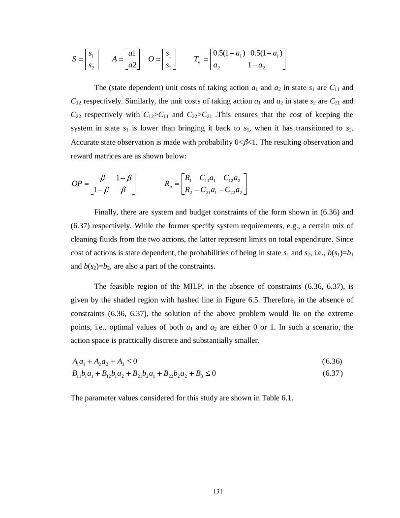
131
2
1
2
1
2
1
s
sO
a
aA
s
sS
22
11
1
)1(5.0)1(5.0
aa
aaTa
The (state dependent) unit costs of taking action a1 and a2 in state s1 are C11 and
C12 respectively. Similarly, the unit costs of taking action a1 and a2 in state s2 are C21 and
C22 respectively with C12>C11 and C22>C21 .This ensures that the cost of keeping the
system in state s1 is lower than bringing it back to s1, when it has transitioned to s2.
Accurate state observation is made with probability 0< <1. The resulting observation and
reward matrices are as shown below:
2221212
2121111
1
1
aCaCR
aCaCRROP a
Finally, there are system and budget constraints of the form shown in (6.36) and
(6.37) respectively. While the former specify system requirements, e.g., a certain mix of
cleaning fluids from the two actions, the latter represent limits on total expenditure. Since
cost of actions is state dependent, the probabilities of being in state s1 and s2, i.e., b(s1)=b1
and b(s2)=b2, are also a part of the constraints.
The feasible region of the MILP, in the absence of constraints (6.36, 6.37), is
given by the shaded region with hashed line in Figure 6.5. Therefore, in the absence of
constraints (6.36, 6.37), the solution of the above problem would lie on the extreme
points, i.e., optimal values of both a1 and a2 are either 0 or 1. In such a scenario, the
action space is practically discrete and substantially smaller.
)37.6(0
)36.6(0
32222122121121111
32211
BabBabBabBabB
AaAaA
The parameter values considered for this study are shown in Table 6.1.
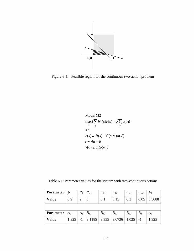
132
0,0 1
1
0,0 1
1
Figure 6.5: Feasible region for the continuous two-action problem
)()(
)'()',()()(
..
})()()({max
M2Model
otpbov
BAat
sassCsRsr
ts
ovsrsb
o
os
o
a
Table 6.1: Parameter values for the system with two-continuous actions
Parameter R1 R2 C11 C12 C21 C22 A1
Value 0.9 2 0 0.1 0.15 0.3 0.05 0.5088
Parameter A2 A3 B11 B12 B21 B22 B3 A2
Value 1.325 -1 3.1185 9.355 3.0736 1.025 -1 1.325
133
The MILP model for the value backups for above example is shown by model
M2. This pertains to value iteration around pre-decision state variable.
Optimal policy and value function
The converged value function and policy for both approaches are shown in Figure
6.6. When the probability of being in state s=1 is sufficiently high, action a1 is executed
whose value depends on the constraints and the objective value. The policy for the two
action problem is rather simple and intuitive. When the probability of being in state s=1
falls below a certain threshold (different for both approaches), action a2 is performed so
that it satisfies the constraints listed in (6.36) and (6.37). As seen in Figure 6.6, the value
function for the enumeration based solution is lower. The performance and solution times
of MILP and enumeration based methods (as a function of number of PERSEUS
iterations) are shown in Figures 6.7(a) and 6.7(d) respectively. The enumeration based
method convergences in an order of magnitude less time than the MILP based method.
However, the performance of the enumeration based method is lower than that of the
MILP solution. This is attributed to the discretization of the action space. The action
corresponding to each gradient vector is also shown in Figure 6.6. As seen, the actions
pertaining to the best solution obtained by enumeration of the value function is limited by
the size of the action space grid. For the same reason, the MILP based method appears to
be converging faster in terms of number of iterations as seen in Figure 6.7(d).
Scalability
To study how the solution time scales with the problem size and understand
whether the value gap depends on the problem size, two additional experiments are
performed: (i) a system with three possible states and three actions, (ii) a system with
four states and four actions. Similar to the two-action system above, the states are discrete
and all actions are continuous and range from 0 to 1. The probability transition matrix is a
linear function of actions and the constraints follow the same linear structure as (6.36)
and (6.37). The parameter values are shown in Table 6.1 and the results are reported in
Table 6.2. It is observed that the performance gap widens as the problem size grows. The
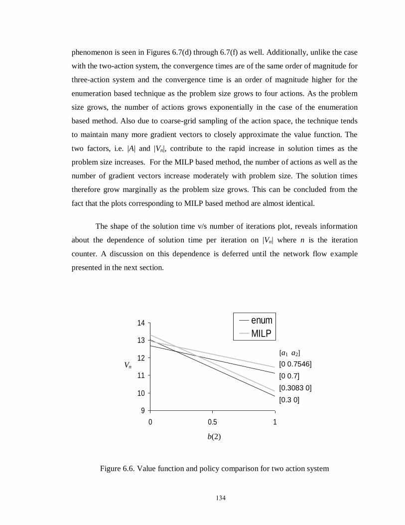
134
phenomenon is seen in Figures 6.7(d) through 6.7(f) as well. Additionally, unlike the case
with the two-action system, the convergence times are of the same order of magnitude for
three-action system and the convergence time is an order of magnitude higher for the
enumeration based technique as the problem size grows to four actions. As the problem
size grows, the number of actions grows exponentially in the case of the enumeration
based method. Also due to coarse-grid sampling of the action space, the technique tends
to maintain many more gradient vectors to closely approximate the value function. The
two factors, i.e. |A| and |Vn|, contribute to the rapid increase in solution times as the
problem size increases. For the MILP based method, the number of actions as well as the
number of gradient vectors increase moderately with problem size. The solution times
therefore grow marginally as the problem size grows. This can be concluded from the
fact that the plots corresponding to MILP based method are almost identical.
The shape of the solution time v/s number of iterations plot, reveals information
about the dependence of solution time per iteration on |Vn| where n is the iteration
counter. A discussion on this dependence is deferred until the network flow example
presented in the next section.
9
10
11
12
13
14
0 0.5 1
b(2)
Vn
enum
MILP
Figure 6.6. Value function and policy comparison for two action system
[0.3 0]
[0 0.7]
[0.3083 0]
[0 0.7546]
[a1 a2]
Vn
b(2)
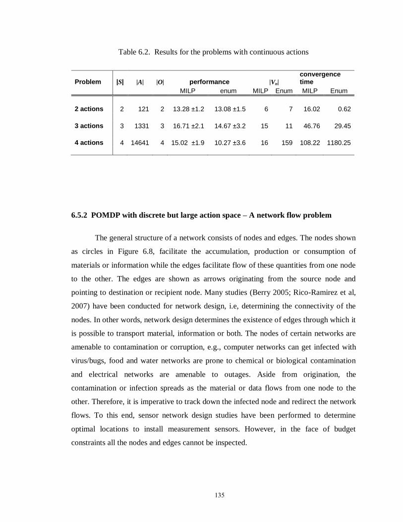
135
Table 6.2. Results for the problems with continuous actions
Problem |S| |A| |O| performance |Vn|
convergence time
MILP enum MILP Enum MILP Enum
2 actions 2 121 2 13.28 ±1.2 13.08 ±1.5 6 7 16.02 0.62
3 actions 3 1331 3 16.71 ±2.1 14.67 ±3.2 15 11 46.76 29.45
4 actions 4 14641 4 15.02 ±1.9 10.27 ±3.6 16 159 108.22 1180.25
6.5.2 POMDP with discrete but large action space – A network flow problem
The general structure of a network consists of nodes and edges. The nodes shown
as circles in Figure 6.8, facilitate the accumulation, production or consumption of
materials or information while the edges facilitate flow of these quantities from one node
to the other. The edges are shown as arrows originating from the source node and
pointing to destination or recipient node. Many studies (Berry 2005; Rico-Ramirez et al,
2007) have been conducted for network design, i.e, determining the connectivity of the
nodes. In other words, network design determines the existence of edges through which it
is possible to transport material, information or both. The nodes of certain networks are
amenable to contamination or corruption, e.g., computer networks can get infected with
virus/bugs, food and water networks are prone to chemical or biological contamination
and electrical networks are amenable to outages. Aside from origination, the
contamination or infection spreads as the material or data flows from one node to the
other. Therefore, it is imperative to track down the infected node and redirect the network
flows. To this end, sensor network design studies have been performed to determine
optimal locations to install measurement sensors. However, in the face of budget
constraints all the nodes and edges cannot be inspected.
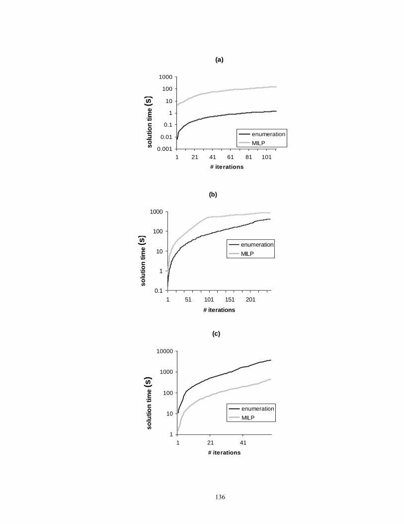
136
(a)
0.001
0.01
0.1
1
10
100
1000
1 21 41 61 81 101
# iterations
so
luti
on
tim
e
(s)
enumeration
MILP
(b)
0.1
1
10
100
1000
1 51 101 151 201
# iterations
so
luti
on
tim
e
(s)
enumeration
MILP
(c)
1
10
100
1000
10000
1 21 41
# iterations
so
luti
on
tim
e
(s)
enumeration
MILP
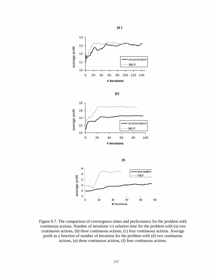
137
Figure 6.7. The comparison of convergence times and performance for the problem with
continuous actions. Number of iterations v/s solution time for the problem with (a) two
continuous actions, (b) three continuous actions, (c) four continuous actions. Average
profit as a function of number of iterations for the problem with (d) two continuous
actions, (e) three continuous actions, (f) four continuous actions.
avg profit
(d )
10
11
12
13
14
0 20 40 60 80 100 120 140
# iterations
ave
rag
e p
rofit
enumeration
MILP
(e)
10
12
14
16
18
0 20 40 60 80 100
# iterations
ave
rag
e p
rofit
enumeration
MILP
avera
ge p
rofit
avera
ge p
rofit
avera
ge p
rofit
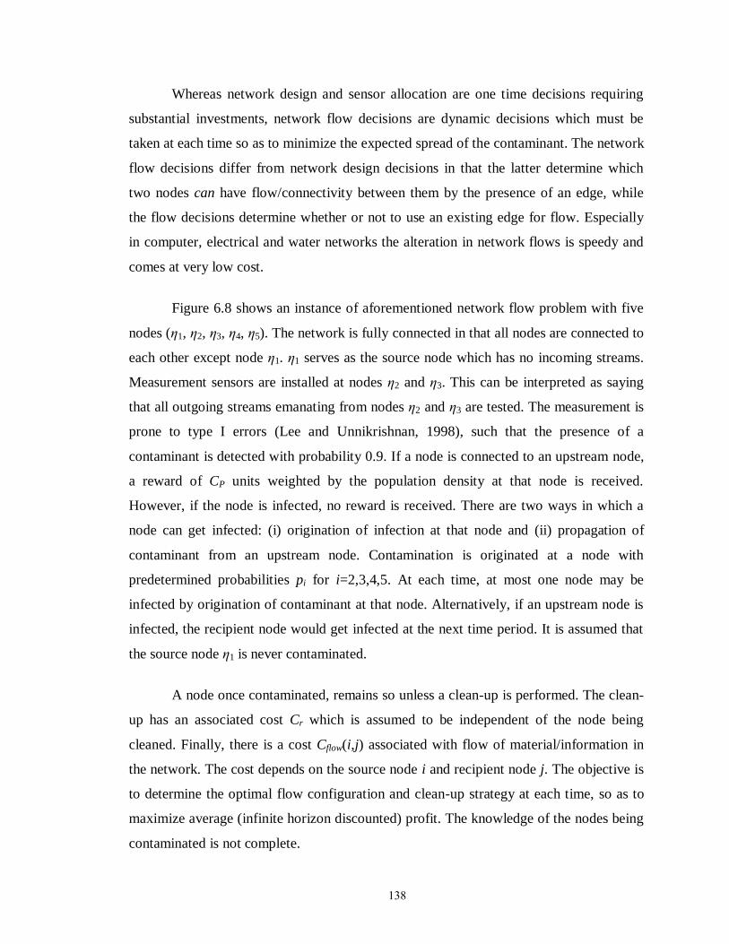
138
Whereas network design and sensor allocation are one time decisions requiring
substantial investments, network flow decisions are dynamic decisions which must be
taken at each time so as to minimize the expected spread of the contaminant. The network
flow decisions differ from network design decisions in that the latter determine which
two nodes can have flow/connectivity between them by the presence of an edge, while
the flow decisions determine whether or not to use an existing edge for flow. Especially
in computer, electrical and water networks the alteration in network flows is speedy and
comes at very low cost.
Figure 6.8 shows an instance of aforementioned network flow problem with five
nodes (ε1, ε2, ε3, ε4, ε5). The network is fully connected in that all nodes are connected to
each other except node ε1. ε1 serves as the source node which has no incoming streams.
Measurement sensors are installed at nodes ε2 and ε3. This can be interpreted as saying
that all outgoing streams emanating from nodes ε2 and ε3 are tested. The measurement is
prone to type I errors (Lee and Unnikrishnan, 1998), such that the presence of a
contaminant is detected with probability 0.9. If a node is connected to an upstream node,
a reward of CP units weighted by the population density at that node is received.
However, if the node is infected, no reward is received. There are two ways in which a
node can get infected: (i) origination of infection at that node and (ii) propagation of
contaminant from an upstream node. Contamination is originated at a node with
predetermined probabilities pi for i=2,3,4,5. At each time, at most one node may be
infected by origination of contaminant at that node. Alternatively, if an upstream node is
infected, the recipient node would get infected at the next time period. It is assumed that
the source node ε1 is never contaminated.
A node once contaminated, remains so unless a clean-up is performed. The clean-
up has an associated cost Cr which is assumed to be independent of the node being
cleaned. Finally, there is a cost Cflow(i,j) associated with flow of material/information in
the network. The cost depends on the source node i and recipient node j. The objective is
to determine the optimal flow configuration and clean-up strategy at each time, so as to
maximize average (infinite horizon discounted) profit. The knowledge of the nodes being
contaminated is not complete.
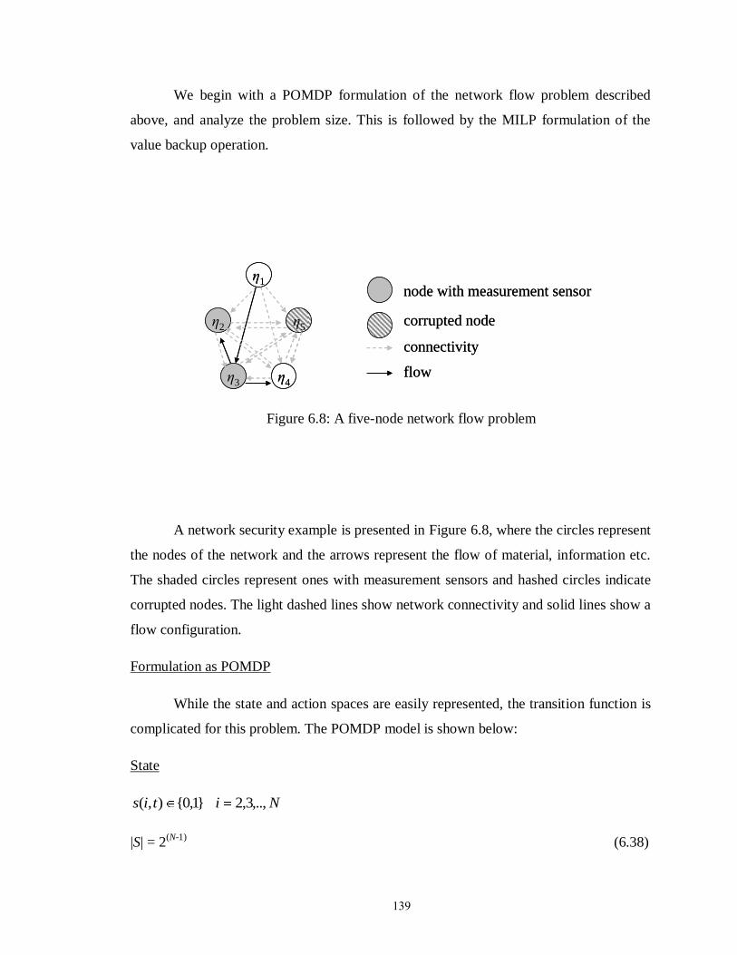
139
We begin with a POMDP formulation of the network flow problem described
above, and analyze the problem size. This is followed by the MILP formulation of the
value backup operation.
ε2
ε3 ε4
ε5
ε1node with measurement sensor
connectivity
flow
corrupted nodeε2
ε3 ε4
ε5
ε1node with measurement sensor
connectivity
flow
corrupted node
Figure 6.8: A five-node network flow problem
A network security example is presented in Figure 6.8, where the circles represent
the nodes of the network and the arrows represent the flow of material, information etc.
The shaded circles represent ones with measurement sensors and hashed circles indicate
corrupted nodes. The light dashed lines show network connectivity and solid lines show a
flow configuration.
Formulation as POMDP
While the state and action spaces are easily represented, the transition function is
complicated for this problem. The POMDP model is shown below:
State
Nitis ,..,3,2}1,0{),(
|S| = 2(N-1)
(6.38)
140
The size of state space is given by (6.38) where N is the number of nodes in the network
Action
Nitia
NjNitjia
repair
flow
,...,3,2}1.0{),(
,..,3,2;,..,2,1}1,0{),,(
The term aflow(i,i) for i=2,3,..,N is the node activation term. aflow(i,i)=1 implies that node i
is connected indicating that it has a positive inflow from some other node in the network.
aflow(1,1) is always 1.
|A| = 2N(N-1)
+2(N-1)
(6.39)
The expression for the size of the action space in (6.39) suggests a very large action space
for even small values of N. However, many actions are not feasible. E.g.
(i) A node with no inflow cannot have any outflow or accumulation
(ii) A node with positive inflow must have either accumulation or outflow
(iii) A node can be either upstream or downstream of another node but not both.
(iv) Each node must have at most one supply node.
The above constraints reduce the size of the action space considerably.
State transition function
Given the state and action at the current time, the state at the next time may be
determined by the following relations:
(i) Contamination by origination – A node i is contaminated by origination
depending on the contamination probability pi. This is shown in (6.40), where
p(t+1) is the realization of probability of origination of contamination and
δ(.)=1 if the condition within the parenthesis is met.
5,..,3,2))1(()1,( iforptptis i (6.40)
141
(ii) Contamination by propagation – If a source node k is contaminated, recipient
node i will contaminated at the next time period (6.41).
5,..,3,2;5,..,3,2),,(),()1,( kifortikatkstis flow (6.41)
(iii) Carried over contamination – If node i is contaminated and not repaired at the
current time, it will be contaminated at the next time period (6.42).
5,..,3,2}0),,(),(max{)1,( ifortiatistis repair (6.42)
The state transition matrix for contamination by origination is a static matrix
independent of current state and action. This constant matrix is designated as map1. The
transition matrices that account for points (ii) and (iii) above need to be determined for
each state action pair. The matrix that combines the effects of factors (ii) and (iii) is
designated by map2. Therefore, the post decision belief state is given by (6.43).
)',()',()()'(}{
21 ssmapssmapsbsba
Ss
a (6.43)
Observation space and observation probability matrix
itio }1,0{),(
||2|| MO (6.44)
The size of observation space is given by (6.44) where M is the set of nodes with
measurement sensors. It is assumed that all measurement sensors can sense the
presence of a contaminant 90% of the time. The observation probability matrix
reflects this fact. E.g. if the measurement sensors are installed at nodes η2 and η3, the
possible observations are:
}1,1{};1,0{};0,1{;}0,0{)},3(),,2({ toto
142
When nodes ε2 and ε3 are both contaminated, i.e., s(2,t)=s(3,t)=1, the observation
probabilities are given by:
2
2
9.0})1,1{)},3(),,2(({
9.0)9.01(})1,0{)},3(),,2(({
)9.01(9.0})0,1{)},3(),,2(({
)9.01(})0,0{)},3(),,2(({
totop
totop
totop
totop
The observation probabilities for the other states may be calculated in a similar
manner.
Profit/reward Function
The profit function at time t comprises of the following terms
(i) Reward for active non-contaminated nodes – This is given by the first term in
(6.45)
(ii) Cost of flow and repair actions – This is given by the second and third terms
in (6.45).
i
repairrepair
j i
flowflowflow
i
iPt
tiaiC
tjiajiCtistiiawCasr
),()(
),,(),(),(),,(),(
(6.45)
The value backups using enumeration are straightforward once the transition matrices
are developed for each action. The MILP for value backups, however, is more
involved. This is discussed below:
MILP based value backups
The MILP formulation must account for the following
(i) The constraints to exclude infeasible actions
(ii) The equations to develop state transition matrix map2 as a function of actions.
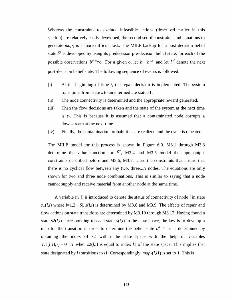
143
Whereas the constraints to exclude infeasible actions (described earlier in this
section) are relatively easily developed, the second set of constraints and equations to
generate map2 is a more difficult task. The MILP backup for a post-decision belief
state a is developed by using its predecessor pre-decision belief state, for each of the
possible observations ob oa, . For a given o, let oabb , and let a′ denote the next
post-decision belief state. The following sequence of events is followed:
(i) At the beginning of time t, the repair decision is implemented. The system
transitions from state s to an intermediate state s1.
(ii) The node connectivity is determined and the appropriate reward generated.
(iii) Then the flow decisions are taken and the state of the system at the next time
is s2. This is because it is assumed that a contaminated node corrupts a
downstream at the next time.
(iv) Finally, the contamination probabilities are realized and the cycle is repeated.
The MILP model for this process is shown in Figure 6.9. M3.1 through M3.3
determine the value function for a′, M3.4 and M3.5 model the input-output
constraints described before and M3.6, M3.7, .. are the constraints that ensure that
there is no cyclical flow between any two, three,..N nodes. The equations are only
shown for two and three node combinations. This is similar to saying that a node
cannot supply and receive material from another node at the same time.
A variable z(l,i) is introduced to denote the status of connectivity of node i in state
s1(l,i) where l=1,2,..|S|. z(l,i) is determined by M3.8 and M3.9. The effects of repair and
flow actions on state transitions are determined by M3.10 through M3.12. Having found a
state s2(l,i) corresponding to each state s(l,i) in the state space, the key is to develop a
map for the transition in order to determine the belief state ba′. This is determined by
obtaining the index of s2 within the state space with the help of variables
iill 0),1,(. when s2(l,i) is equal to index l1 of the state space. This implies that
state designated by l transitions to l1. Correspondingly, map2(l,l1) is set to 1. This is
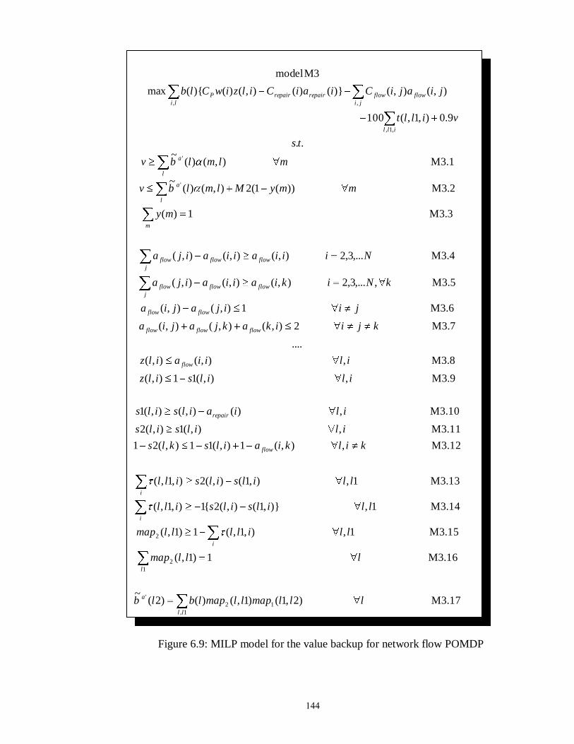
144
17.3M)2,1()1,()()2(~
16.3M1)1,(
15.3M1,),1,(1)1,(
14.3M1,)},1(),(2{1),1,(
13.3M1,),1(),(2),1,(
12.3M,),(1),(11),(21
11.3M,),(1),(2
10.3M,)(),(),(1
9.3M,),(11),(
8.3M,),(),(
....
7.3M2),(),(),(
6.3M1),(),(
5.3M,,...3,2),(),(),(
4.3M,...3,2),(),(),(
3.3M1)(
2.3M))(1(2),()(~
1.3M),()(~
..
9.0),1,(100
),(),()}()(),()(){(max
M3model
1,
12
'
1
2
2
'
'
,1,
,,
lllmapllmaplblb
lllmap
llillllmap
llilsilsill
llilsilsill
kilkiailskls
ililsils
iliailsils
ililsilz
iliiailz
kjiikakjajia
jiijajia
kNikiaiiaija
Niiiaiiaija
my
mmyMlmlbv
mlmlbv
ts
villt
jiajiCiaiCilziwClb
ll
a
l
i
i
i
flow
repair
flow
flowflowflow
flowflow
flowflow
j
flow
flowflow
j
flow
m
l
a
l
a
ill
flow
ji
flowrepair
li
repairP
Figure 6.9: MILP model for the value backup for network flow POMDP
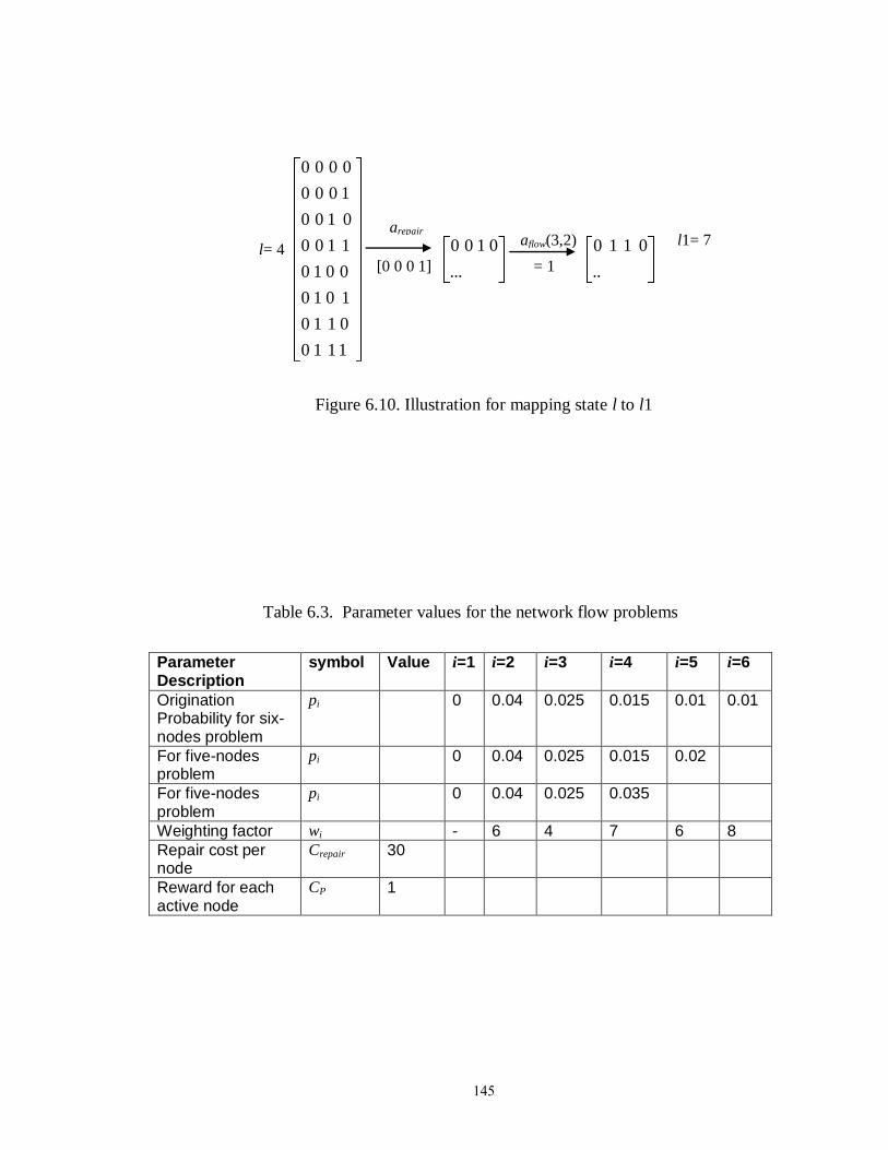
145
..
0110
...
0100
1110
0110
1010
0010
1100
0100
1000
0000
Figure 6.10. Illustration for mapping state l to l1
Table 6.3. Parameter values for the network flow problems
Parameter Description
symbol Value i=1 i=2 i=3 i=4 i=5 i=6
Origination Probability for six-nodes problem
pi 0 0.04 0.025 0.015 0.01 0.01
For five-nodes problem
pi 0 0.04 0.025 0.015 0.02
For five-nodes problem
pi 0 0.04 0.025 0.035
Weighting factor wi - 6 4 7 6 8
Repair cost per node
Crepair 30
Reward for each active node
CP 1
l= 4 l1= 7
arepair
aflow(3,2)
[0 0 0 1]
= 1
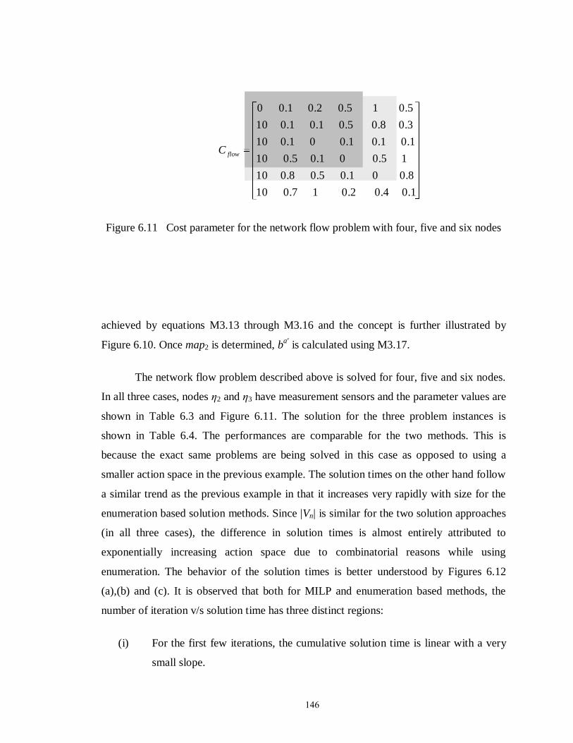
146
0.1 0.4 0.2 1 0.7 10
0.8 0 0.1 0.5 0.8 10
1 0.5 0 0.1 0.5 10
0.1 0.1 0.1 0 0.1 10
0.3 0.8 0.5 0.1 0.1 10
0.5 1 0.5 0.2 0.1 0
flowC
Figure 6.11 Cost parameter for the network flow problem with four, five and six nodes
achieved by equations M3.13 through M3.16 and the concept is further illustrated by
Figure 6.10. Once map2 is determined, ba′ is calculated using M3.17.
The network flow problem described above is solved for four, five and six nodes.
In all three cases, nodes ε2 and ε3 have measurement sensors and the parameter values are
shown in Table 6.3 and Figure 6.11. The solution for the three problem instances is
shown in Table 6.4. The performances are comparable for the two methods. This is
because the exact same problems are being solved in this case as opposed to using a
smaller action space in the previous example. The solution times on the other hand follow
a similar trend as the previous example in that it increases very rapidly with size for the
enumeration based solution methods. Since |Vn| is similar for the two solution approaches
(in all three cases), the difference in solution times is almost entirely attributed to
exponentially increasing action space due to combinatorial reasons while using
enumeration. The behavior of the solution times is better understood by Figures 6.12
(a),(b) and (c). It is observed that both for MILP and enumeration based methods, the
number of iteration v/s solution time has three distinct regions:
(i) For the first few iterations, the cumulative solution time is linear with a very
small slope.

147
(ii) After this, the solution time grows exponentially with iteration count.
(iii) Finally, it becomes linear again with a large slope.
This is because the value function is initialized with a single gradient vector and the value
function is set to the lowest possible reward. Due to this reason, a single update improves
the value function for the entire sampled belief set. Consequently, only a single gradient
vector comprises the value function for the first few iterations leading to same solution
time per iteration. Beyond this point, the size of the value function, i.e., the number of
gradient vectors during each iteration increase as the shape of the value function begins to
take form. This causes the solution time to increase per iteration, as more gradient vectors
are added. Finally, the value function converges and no new gradient vectors are added.
At this point, the solution time again becomes constant for each iteration. The time per
iteration is much higher as compared to that for the initial iterations.
Finally, the convergence of value function is depicted in Figure 6.13 (a) and (b)
for the four and five node problems respectively. The average performance is plotted as a
function of solution time. For the four node network flow problem, the value function
converges faster for the enumeration based method. But the phenomenon is reversed for
the five node problem. As seen from Table 6.4, the performance of the MILP based
method only gets better with increase problem size.
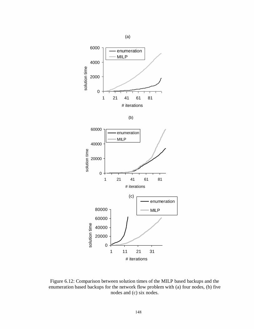
148
Figure 6.12: Comparison between solution times of the MILP based backups and the
enumeration based backups for the network flow problem with (a) four nodes, (b) five
nodes and (c) six nodes.
(a)
0
2000
4000
6000
1 21 41 61 81
# iterations
solu
tion tim
e (s
)
enumeration
MILP
(b)
0
20000
40000
60000
1 21 41 61 81
# iterations
solu
tion t
ime
(s)
enumeration
MILP
(c)
0
20000
40000
60000
80000
1 11 21 31
# iterations
so
lutio
n t
ime
(s
)
enumeration
MILP
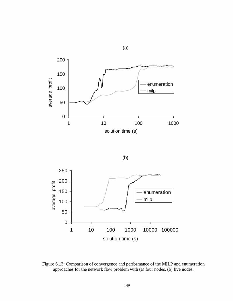
149
Figure 6.13: Comparison of convergence and performance of the MILP and enumeration
approaches for the network flow problem with (a) four nodes, (b) five nodes.
(a)
0
50
100
150
200
1 10 100 1000
solution time (s)
avera
ge p
rofit
enumeration
milp
(b)
0
50
100
150
200
250
1 10 100 1000 10000 100000
solution time (s)
ave
rag
e p
rofit
enumeration
milp
ave
rag
e p
rofit
ave
rag
e p
rofit
ave
rag
e p
rofit
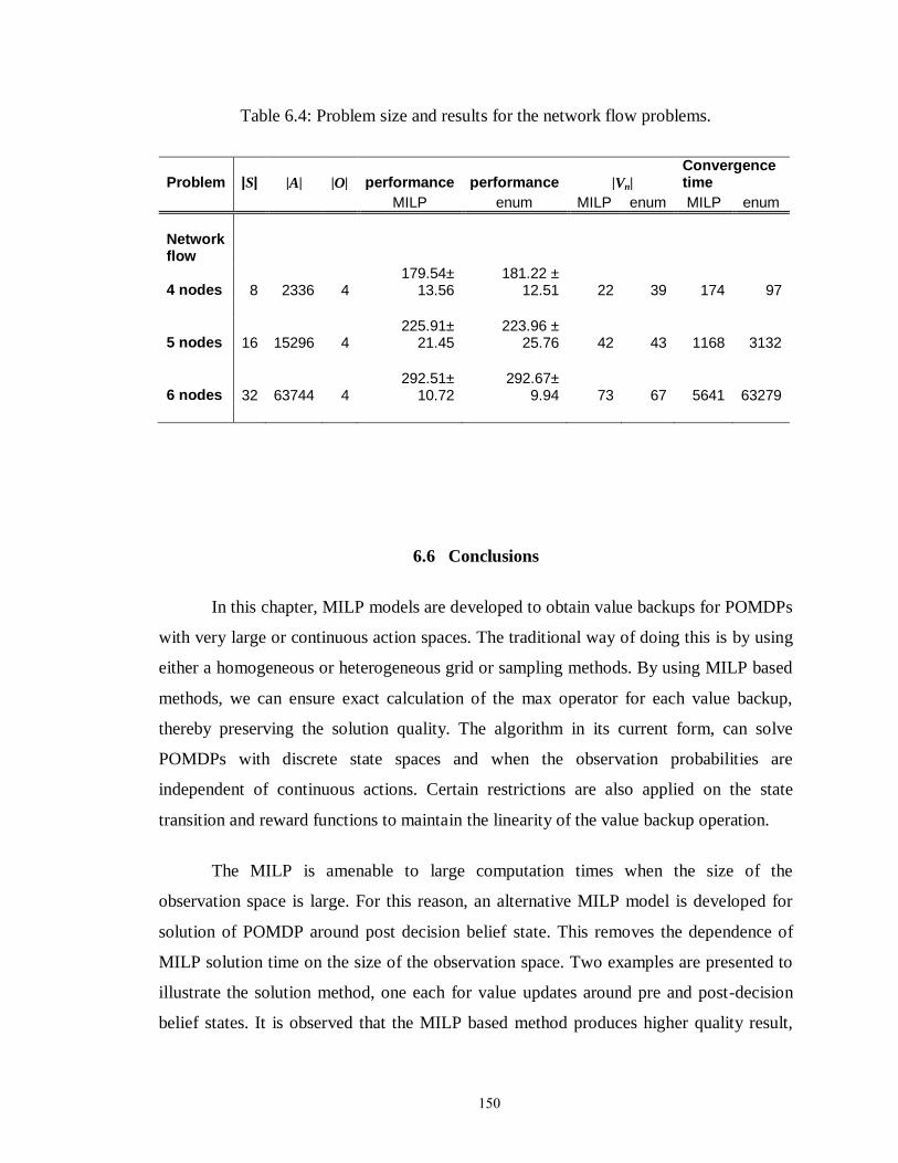
150
Table 6.4: Problem size and results for the network flow problems.
Problem |S| |A| |O|
performance
performance |Vn|
Convergence time
MILP enum MILP enum MILP enum
Network flow
4 nodes 8 2336 4 179.54±
13.56 181.22 ±
12.51 22 39 174 97
5 nodes 16 15296 4 225.91±
21.45 223.96 ±
25.76 42 43 1168 3132
6 nodes 32 63744 4 292.51±
10.72 292.67±
9.94 73 67 5641 63279
6.6 Conclusions
In this chapter, MILP models are developed to obtain value backups for POMDPs
with very large or continuous action spaces. The traditional way of doing this is by using
either a homogeneous or heterogeneous grid or sampling methods. By using MILP based
methods, we can ensure exact calculation of the max operator for each value backup,
thereby preserving the solution quality. The algorithm in its current form, can solve
POMDPs with discrete state spaces and when the observation probabilities are
independent of continuous actions. Certain restrictions are also applied on the state
transition and reward functions to maintain the linearity of the value backup operation.
The MILP is amenable to large computation times when the size of the
observation space is large. For this reason, an alternative MILP model is developed for
solution of POMDP around post decision belief state. This removes the dependence of
MILP solution time on the size of the observation space. Two examples are presented to
illustrate the solution method, one each for value updates around pre and post-decision
belief states. It is observed that the MILP based method produces higher quality result,

151
when the entire action space is not considered for enumeration based method. The
solution gap increases with problem size.
Additionally, the solution time scales linearly with problem size for the MILP
based method, while it grows exponentially in case of enumeration based methods. This
is attributed to the exponential increase in the size of action space due to combinatorial
reasons. Consequently, the MILP quickly surpasses the enumeration based methods in
terms of lower solution times and better solution quality as the problem size is increased.
This makes the MILP based solution very well suited for POMDPs with high
dimensional actions and continuous actions.
152
CHAPTER 7
CONTRIBUTIONS AND FUTURE WORK
7.1 Conclusions and Contributions
Optimal resource management is an integral part of any manufacturing
environment. This body of work is a step forward in devising better resource
management policies in conjunction with production, inspection or distribution strategies.
This is performed for three different types of resource degradation models spanning many
process industries. From an academic standpoint, this thesis seeks to make contributions
in the following areas:
Introduction of a new class of problems
In Chapters 3 and 4, a new class of problems, the inventory control of perishable
resources is considered. The study is aimed at resources that get consumed, break or exit
the system, with time scales comparable to that of production. Aside from small and
specialized manufacturing equipment, the technique can be extended to human resource
management in the form of hiring and training decisions.
The inventory of perishable resources is directly affected by two important
factors: (i) the procurement policy which adds to the inventory (ii) the production
process, whereby the resources age and break, resulting in depletion of inventory. It is
obvious then, that the production decisions directly affect the resource management
decisions. The availability of resources, on the other hand, place constraints of production
quantities. These inter-dependent decisions are considered as a part of a combined
optimization problem presented in Chapter 3. It is shown by numerical examples that the
performance is significantly better when the resource management decisions are
considered together with production planning as opposed to independent of it. The
performance gap depends on the level to which the resource breaking rate is affected by
153
usage, average resource life and variability in the total number of resources used per time
period.
When the system is plagued by high level of uncertainty, the problem is
reformulated as an MDP and solved using approximate dynamic programming (ADP) in
Chapter 4. For the deterministic problem and for the parameter set considered, the
solution obtained by the ADP algorithm is 94.5% of the optimal solution. For the
stochastic demand and resource life models, the ADP algorithm proves to be a more
flexible and widely applicable choice. This is because the ADP algorithm is capable of
taking a more comprehensive view of the uncertainty, thereby taking improved and more
informed decisions as compared to the rolling horizon methodology.
Practical extension to an existing problem
Randomly deteriorating machines with limited observability, have been
traditionally solved as partially observable Markov decision processes. In Chapter 5, this
work is extended by considering multiple machines and multiple types of jobs being
operated on the machine. The study is motivated, in part, by the recent advancements in
efficient solution of medium to large size POMDPs.
Costly inspections dissuade the decision-maker to test all the processed jobs
generating a possibility of propagation and accumulation of defective items. Therefore,
information on defective items needs to be maintained at all times. This results in a
significantly larger state space and consequently, the overall POMDP. An approximate
solution method called PERSEUS (Spaan and Vlassis, 2005) is used for the solution of
POMDPs. Structure of the optimal policy and that of the value function is studied. While
the treatment of the above problem as a POMDP is shown to offer promise in terms of
better performance over heuristic rules, the characterization of either the optimal policy
or value function or both is required, so that solutions to problems of practical scale can
be obtained. This point is discussed further in section 7.2.
Algorithmic Development
While point based algorithms for solution of POMDPs prove efficient with
discrete or small action spaces, literature on large action spaces is limited to action-
154
sampling based algorithms. Whereas, this might be a successful strategy for some
problems, it is difficult to devise sampling schemes for many applications. In Chapter 6,
we introduce the notion of obtaining Bellman updates or value backups using a mixed
integer mathematical programming (MILP) model. The MILP based backups are made
possible by the piecewise linear and convex value function and certain requirements on
reward and probability functions. The latter essentially ensure a linear model.
Recognizing that a large size observation space significantly increases the
solution time of MILP, we present an alternative formulation of POMDP around post-
decision belief state. In the latter case, dependence of MILP on the size of observation
space is removed.
The algorithmic strategy is tested on two example problems, one with continuous
actions and the other with discrete but very large action space. It is seen that the MILP
based approach quickly surpasses the enumeration based methods in terms of lower
solution times and/or better solution quality as the problem size is increased. This makes
the MILP based solution very well suited for POMDPs with high dimensional actions and
continuous actions.
7.2 Future Work
There are several avenues along which the current work can be improved or
extended. Some of these are noted below:
Macroeconomic objectives
The combined decision-making in all the problems is performed with the
objective of maximizing a measure of profit. In manufacturing environments, typical
objectives aside from maximizing profit are maximizing cycle time, maximizing
throughput or minimizing tardiness. These objectives would require other considerations,
thereby making the problem richer and more practical.
155
Characterization of optimal policy
For inventory control problems as well as maintenance problems for a single
randomly deteriorating system, the existence of parametric form of optimal policy has
been proven (given that certain conditions are met). It has been shown that for the
inventory control problem and fully observable maintenance problem, the optimal policy
has a control limit structure. For the partially observable machine maintenance problem,
the optimal policy is marginally monotone in the belief space. These findings simplify the
search for optimal policy parameters for large size problems, without having to solve the
actual optimization problem using rigorous methods.
For the extensions presented in this work, it may be possible to find simplified
instances or subclasses of problems for which characterization of optimal policy using a
parametric form can be performed. Additionally, the structure of the value function for
the (single) machine maintenance problem is shown to be marginally monotone (when
certain conditions are met). A good strategy will be to add features to the single machine
problem so that the form of the value function is preserved. Problems developed using
this bottom-up approach would enable use of faster algorithms that take advantage of the
known structure of the value function.
Improvements in MILP based updates for POMDPs
Since an MILP is solved for each value backup, it is required that the model be
computationally sound. In Chapter 6, the MILP formulation involves the big-M type
constraints which potentially slow down the computation. A stronger formulation may
result in significant improvements in MILP solution time.
Continuous state spaces
Presence of continuous actions in a POMDP is often coupled with continuous
states. The algorithm developed in Chapter 6 can only work with discrete states. In point
based algorithms, continuous states are handled using Gaussian mixtures (Spaan, 2006)
in the spirit similar to particle filters. Further research is required to determine if the
MILP based backups may be extended to POMDPs with continuous states
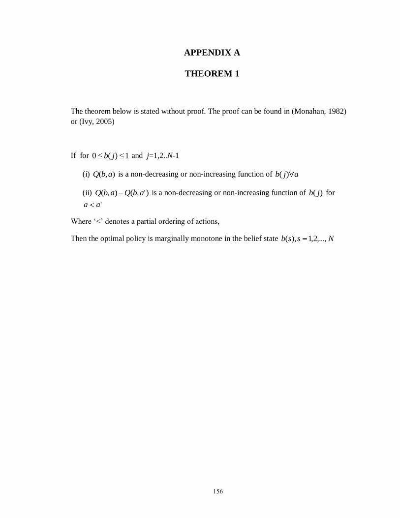
156
APPENDIX A
THEOREM 1
The theorem below is stated without proof. The proof can be found in (Monahan, 1982)
or (Ivy, 2005)
If for 1)(0 jb and j=1,2..N-1
(i) ),( abQ is a non-decreasing or non-increasing function of ajb )(
(ii) )',(),( abQabQ is a non-decreasing or non-increasing function of )( jb for
'aa
Where „<‟ denotes a partial ordering of actions,
Then the optimal policy is marginally monotone in the belief state Nssb ,...,2,1),(
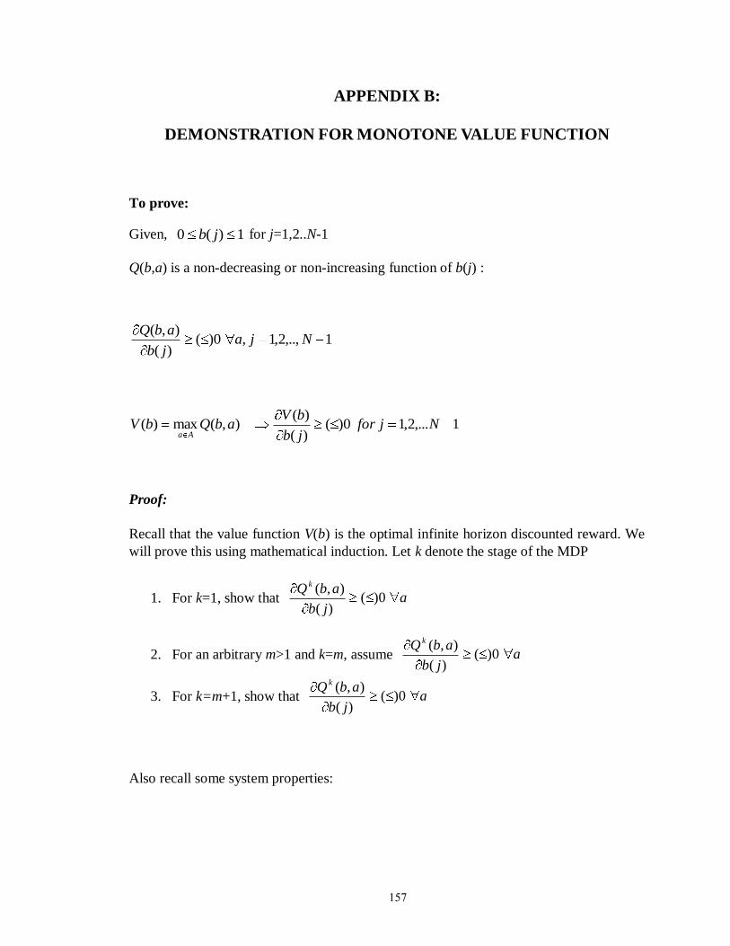
157
APPENDIX B:
DEMONSTRATION FOR MONOTONE VALUE FUNCTION
To prove:
Given, 1)(0 jb for j=1,2..N-1
Q(b,a) is a non-decreasing or non-increasing function of b(j) :
1,..,2,1,0)()(
),(Nja
jb
abQ
1,...2,10)()(
)(),(max)( Njfor
jb
bVabQbV
Aa
Proof:
Recall that the value function V(b) is the optimal infinite horizon discounted reward. We
will prove this using mathematical induction. Let k denote the stage of the MDP
1. For k=1, show that ajb
abQ k
0)()(
),(
2. For an arbitrary m>1 and k=m, assume ajb
abQ k
0)()(
),(
3. For k=m+1, show that ajb
abQ k
0)()(
),(
Also recall some system properties:
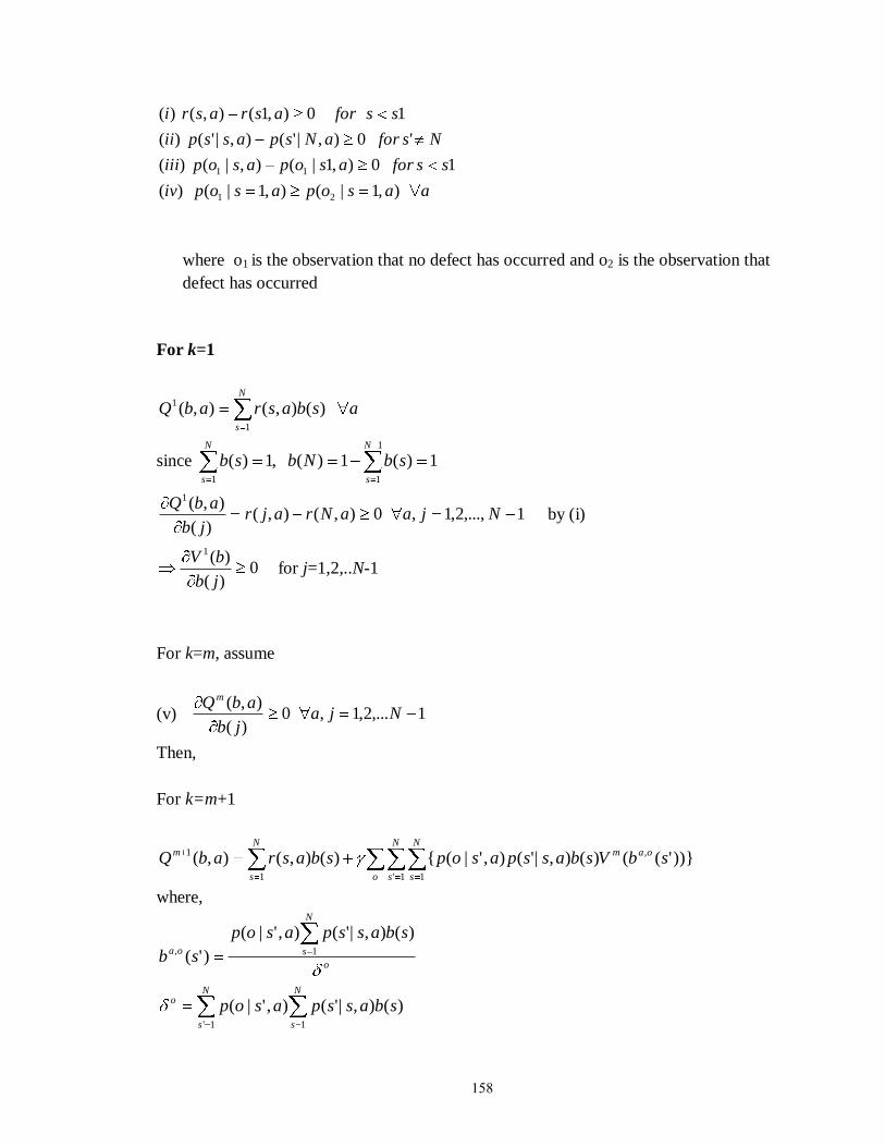
158
aasopasopiv
ssforasopasopiii
NsforaNspasspii
ssforasrasri
),1|(),1|()(
10),1|(),|()(
'0),|'(),|'()(
10),1(),()(
21
11
where o1 is the observation that no defect has occurred and o2 is the observation that
defect has occurred
For k=1
asbasrabQN
s 1
1 )(),(),(
since 1)(1)(,1)(1
11
N
s
N
s
sbNbsb
1,...,2,1,0),(),()(
),(1
NjaaNrajrjb
abQ by (i)
0)(
)(1
jb
bVfor j=1,2,..N-1
For k=m, assume
(v) 1,...2,1,0)(
),(Nja
jb
abQm
Then,
For k=m+1
o
N
s
N
s
oamN
s
m sbVsbasspasopsbasrabQ1' 1
,
1
1 ))}'(()(),|'(),'|({)(),(),(
where,
o
N
soa
sbasspasop
sb 1,
)(),|'(),'|(
)'(
N
s
N
s
o sbasspasop11'
)(),|'(),'|(
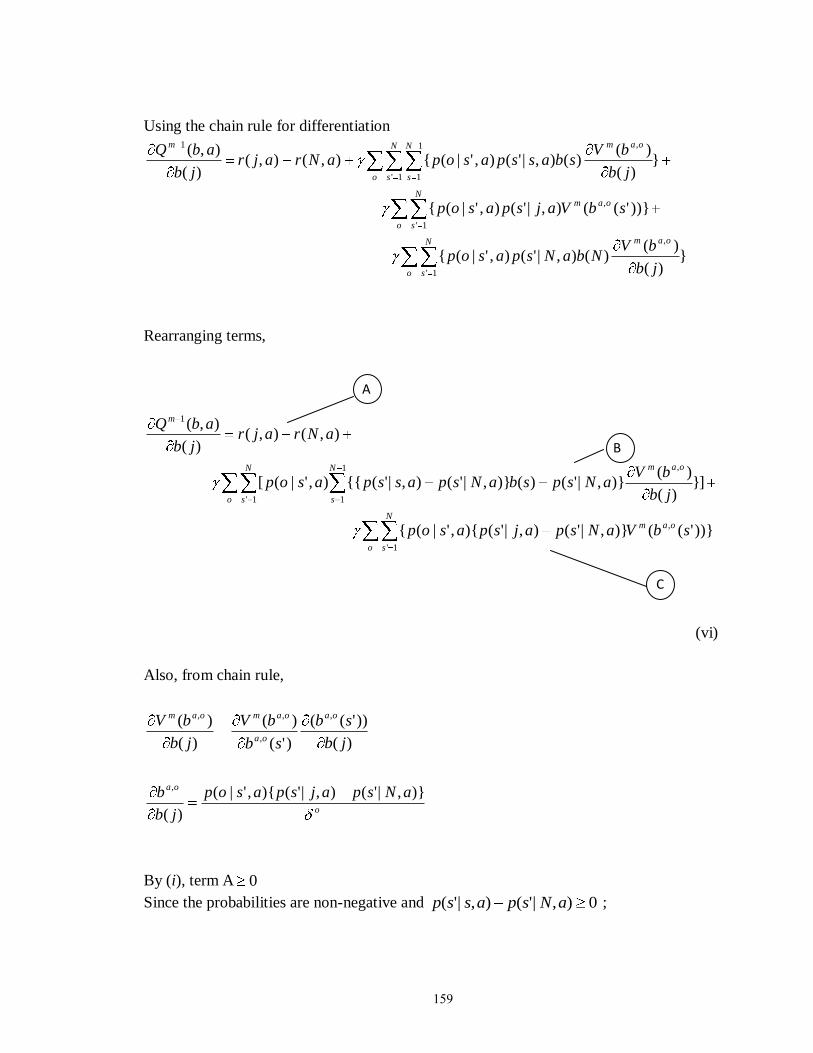
159
Using the chain rule for differentiation
o
N
s
oam
o
N
s
oam
o
N
s
N
s
oamm
jb
bVNbaNspasop
sbVajspasop
jb
bVsbasspasopaNrajr
jb
abQ
1'
,
1'
,
1'
1
1
,1
})(
)()(),|'(),'|({
))}'((),|'(),'|({
})(
)()(),|'(),'|({),(),(
)(
),(
Rearranging terms,
o
N
s
oam
o
N
s
N
s
oam
m
sbVaNspajspasop
jb
bVaNspsbaNspasspasop
aNrajrjb
abQ
1'
,
1'
1
1
,
1
))}'(()},|'(),|'(){,'|({
]})(
)()},|'()()},|'(),|'({{),'|([
),(),()(
),(
(vi)
Also, from chain rule,
)(
))'((
)'(
)(
)(
)( ,
,
,,
jb
sb
sb
bV
jb
bV oa
oa
oamoam
o
oa aNspajspasop
jb
b )},|'(),|'(){,'|(
)(
,
By (i), term A 0
Since the probabilities are non-negative and 0),|'(),|'( aNspassp ;
A
B
C
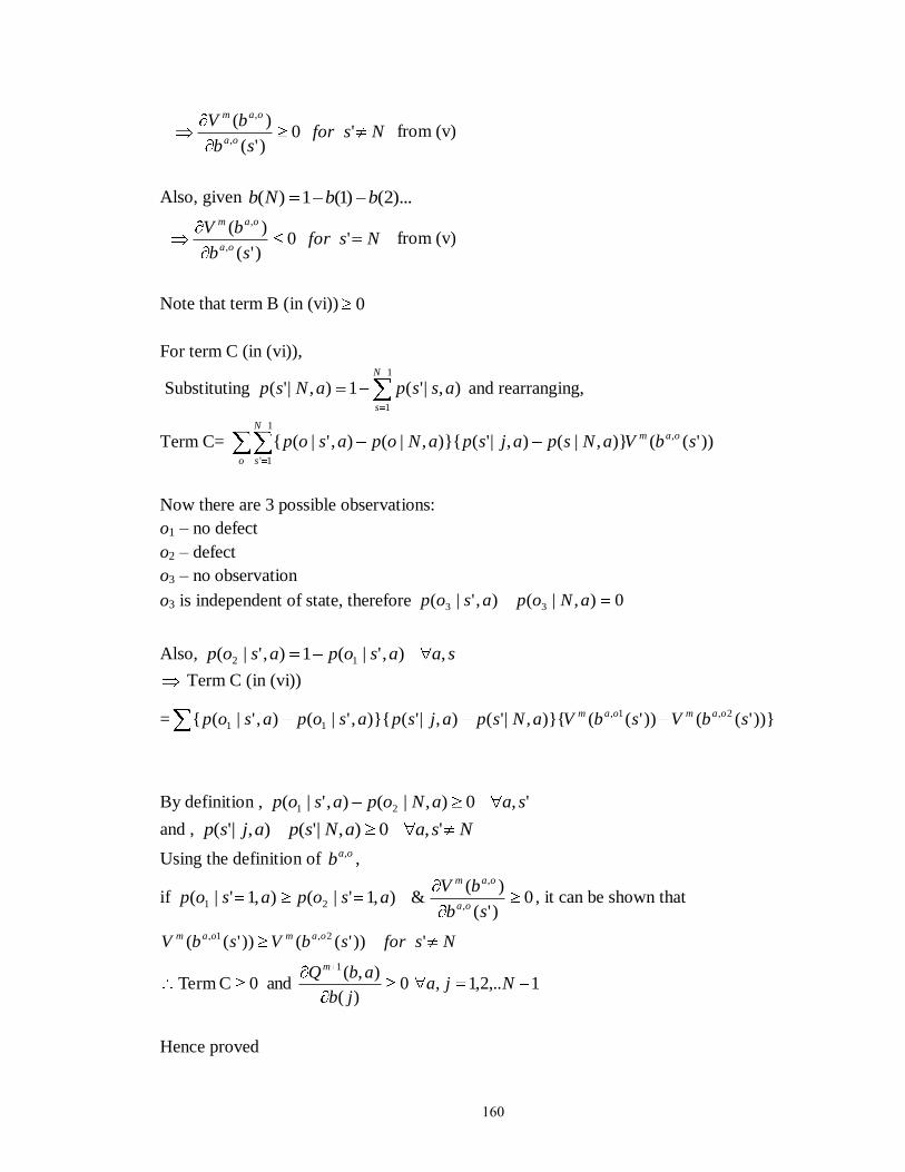
160
Nsforsb
bVoa
oam
'0)'(
)(,
,
from (v)
Also, given )...2()1(1)( bbNb
Nsforsb
bVoa
oam
'0)'(
)(,
,
from (v)
Note that term B (in (vi)) 0
For term C (in (vi)),
Substituting 1
1
),|'(1),|'(N
s
asspaNsp and rearranging,
Term C= o
N
s
oam sbVaNspajspaNopasop1
1'
, ))'(()},|(),|'()}{,|(),'|({
Now there are 3 possible observations:
o1 – no defect
o2 – defect
o3 – no observation
o3 is independent of state, therefore 0),|(),'|( 33 aNopasop
Also, saasopasop ,),'|(1),'|( 12
Term C (in (vi))
= ))}'(())'(()}{,|'(),|'()}{,'|(),'|({ 2,1,
11 sbVsbVaNspajspasopasop oamoam
By definition , ',0),|(),'|( 21 saaNopasop
and , NsaaNspajsp ',0),|'(),|'(
Using the definition of oab , ,
if 0)'(
)(&),1'|(),1'|(
,
,
21sb
bVasopasop
oa
oam
, it can be shown that
NsforsbVsbV oamoam '))'(())'(( 2,1,
1,..2,1,0)(
),(and0CTerm
1
Njajb
abQm
Hence proved
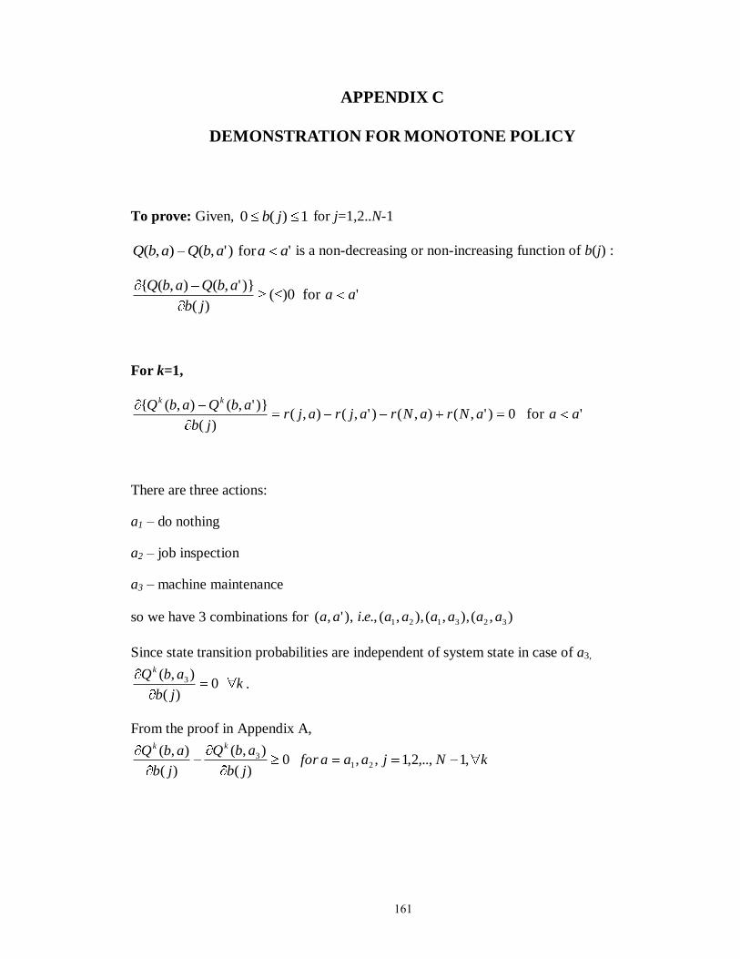
161
APPENDIX C
DEMONSTRATION FOR MONOTONE POLICY
To prove: Given, 1)(0 jb for j=1,2..N-1
'for)',(),( aaabQabQ is a non-decreasing or non-increasing function of b(j) :
'for0)()(
)}',(),({aa
jb
abQabQ
For k=1,
'for0)',(),()',(),()(
)}',(),({aaaNraNrajrajr
jb
abQabQ kk
There are three actions:
a1 – do nothing
a2 – job inspection
a3 – machine maintenance
so we have 3 combinations for ),(),,(),,(.,.),',( 323121 aaaaaaeiaa
Since state transition probabilities are independent of system state in case of a3,
kjb
abQk
0)(
),( 3 .
From the proof in Appendix A,
kNjaaaforjb
abQ
jb
abQkk
,1,..,2,1,,0)(
),(
)(
),(21
3
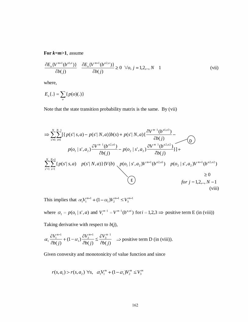
162
For k=m>1, assume
1,..,2,1,0)(
)}({
)(
)}({ ,21,11
Njojb
bVE
jb
bVE oam
o
oam
o (vii)
where,
o
o opE )})(.({{.}
Note that the state transition probability matrix is the same. By (vii)
1,..,2,1
0
)(),'|()(),'|()()}{,|'(),|'({
}])(
)(),'|(
)(
)(),'|(
)(
)(){,|'()()},|'(),|'([{
1'
1
1
2,21
22
1,21
21
2,21
22
1,21
21
3,11
1'
1
1
Njfor
bVasopbVasopbVaNspassp
jb
bVasop
jb
bVasop
jb
bVaNspsbaNspassp
N
s
N
s
oamoam
oamoam
oamN
s
N
s
(viii)
This implies that 1
3
1
21
1
11 )1( mmm VVV
where 3,2,1for)(and),'|( ,11
11 ibVVasop oiamm
i positive term E (in (viii))
Taking derivative with respect to b(j),
)()()1(
)(
1
3
1
21
1
11
jb
V
jb
V
jb
Vmmm
positive term D (in (viii)).
Given convexity and monotonicity of value function and since
mmm VVVsasrasr 3211121 )1(,),(),(
E
D

163
1,..,2,1,0)(
)}({
)(
)}({ ,2,1
Njojb
bVE
jb
bVE oam
o
oam
o
Hence proved
164
REFERENCES
Andrzej, P. and Ruszczyński, A. S. (2003), "Stochastic Programming", Elsevier.
Anthony, R. N. (1965), "Planning and control systems: A framework for analysis"
Harvard University, Boston.
Astrom, K. J. (1965), "Optimal control of Markov decision processes with incomplete
state estimation." Journal of Mathematical Analysis and Applications, 10: 174-
205.
Barto A. G., Bradtko, S. J., Singh S. P. (1995), "Learning to act using real-time dynamic
programming", Artificial Intelligence, 72: 138.
Batson, R. G. and Shishoo, S. (2004), "Algorithm for optimal loss reduction in serial
manufacturing", International Journal of Production Research 42(5).
Bellman, R. (1956), "Dynamic Programming".
Berry, J. W. (2005), "Sensor placement in municipal water networks", Journal of Water
Resources Planning and Management,131(3): 237-243.
Bertsekas, D. P. (1995), "Dynamic Programming and Optimal Control", Athena
Sceineticfic, Belmont, Massachusetts.
Bowling, S. R., Khasawnehb, M. T., Kaewkuekoolc, S. and Cho, B. R. (2004), "A
Markovian approach to determining optimum process target levels for a multi-
stage serial production system", European Journal of Operational Research,
159(3).
Cassady, C. R. and Kutanoglu, E. (2005), "Integrating preventive maintenance planning
and production scheduling for a single machine", IEEE Transactions on
Reliability, 54(2).
165
Cassandra, A. R. (1998), "Exact and Approximate Algorithms for Partially Observable
Markov Decision Processes", Brown University.
Cassandra, A. R., Littman, M. L. and Zhang, N. L. (1997), "Incremental pruning: a
simple,fast, exact algorithm for partially observable Markov decision processes"
in the Proceedings of the Thirteenth Conference on Uncertainty in Artificial
Intelligence.
Chan, K. K. and Spedding, T. A. (2001), "On-line optimization of quality in a
manufacturing system" International Journal of Production Research, 39(6).
Cochran, J. K. and Erol, R. (2001), "Performance modeling of serial production lines
with inspection/repair stations" International Journal of Production Research,
39(8).
De Farias, D. P. and Roy, B. V. (2003), "The linear programming approach to
approximate dynamic programming" Operations Research, 51(6): 850-865.
Derman, C. (1963), "Optimal replacement rules when changes of state are Markovian"
Mathematical Optimization Techniques.
Ding, Y., Ceglarek, D. and Shi, J. (2000), "Modeling and diagnosis of multistage
manufacturing processes: part I - state space model" Japan/USA symposium on
flexible automation.
Ehrenfeld, S. (1976), "On a sequential Markovian decision procedure with incomplete
information" Computers and Operations Research 3: 39-48.
Emmons, H. and Rabinowitz, G. (2003), "Inspection allocation for multistage
deteriorating production systems" IEEE Transactions 24.
Ferris, M. C. (1998), "MATLAB and GAMS: Interfacing Optimization and Visualization
Software" Mathematical Programming Technical Report.
Fishman, G. S. (1996), "Monte Carlo: Concepts, Algorithms, and Applications",
Springer.
166
Girshick, M. and Rubin, H. (1952), "A Bayes' approach to a quality control model"
Annals of Mathematics and Statistics, 23: 114-125.
Grochowski, A., Bhattacharya, D., Viswanathan, T. R. and Laker, K. (1997), "Integrated
circuit testing for quality assurance in manufacturing: history, current status, and
future trends", IEEE Transactions on Circuits and Systems II: Analog and Digital
Signal Processing, 44(8).
Gurnani, H., Drezner, Z. and Akella, R. (1996), "Theory and methodology: Capacity
planning under different inspection strategies", European Journal of Operational
Research 89(2): 302-312.
Haijema R., Val, J. V. and Dijk, N. M. (2004), "Blood Platelet Production: a multi-type
perishable inventory problem", Operations Research Proceedings.
Harrison, J. M. and Meighem V. (1999), "Multi-resource investment strategies:
operational hedging under demand uncertainty", European Journal of Operational
Research.
Hauskretch, M. (2000), "Value-function approximations for partially observable Markov
decision processes" Journal of Artificial Intelligence Research, 13: 33-94.
Heragu, S. S., Graves, R. J., Kim, B. and Onge, A. S. (2002), "Intelligent agent based
framework for manufacturing systems control" IEEE transactions on systems,
man and cybernetics, 32(5).
Hopp, W., Spearman, M. (1996), "Factory Physics: Foundations of Manufacturing
Systems" Irwin, Times mirror.
Huang, Q. and Shi, J. (2004), "Stream of variation modeling and analysis of serial-
parallel multistage manufacturing system" Journal of Manufacturing Science and
Engineering, 126.
Inman, R. R., Blumenfeld, D. E., Ningjian, H. and Li, H. (2003), "Designing production
systems for quality: research opportunities from an automotive industry
perspective" International Journal of Production Research, 41(9).
167
Pineau, J., Gordon, G., Thrun, S. (2003), "Point-based value iteration: An anytime
algorithm for POMDPs" International Jt. Conference on Artificial Intelligence
Ivy, J. S. and Pollak, S. M. (2005), "Marginally monotonic maintenance policies for a
multi-state deteriorating machine with probabilistic monitoring, and silent
failures" IEEE Transactions on Reliability, 54(3): 9.
Kaelbling, L. P., Littman, M. L., and Cassandra, A. R. (1999), "Planning and acting in
partially observable stochastic domains" Artificial Intelligence, 101: 99-134.
Kakade, V., Valenzuela, J. F. and Smith, J. S. (2004), "An optimization model for
selective inspection in serial manufacturing systems" International Journal of
Production Research, 42(18).
Khan, A., Ceglarek, D., Shi, J., Ni, J. and Woo, T. C. (1999), "Sensor optimization for
fault diagnosis in single fixture systems." in the Transactions of ASME, Journal
of Manufacturing Science and Engineering, 120: 109-117.
Kirkpatrick, S., Gelatt, C. D., Vecchi, M. P. (1983), "Optimization by simulated
annealing" Science, New Series 220(4598): 671-680.
Kumar, N., Kennedy, K., Gildersleeve, K., Abelson, R., Masterangelo, C. M. and
Montgomery, D. C. (2006), "A review of yield modeling techniques for
semiconductor manufacturing", International Journal of Production Research,
44(23).
Lee, H. Y. and Apley, D. W. (2004), "Diagnosing manufacturing variation using second
order and fourth order statistics." International Journal of Flexible Manufacturing
Systems 16.
Lee, J. and Unnikrishnan, S. (1998), "Planning quality inspection operations in multistage
manufacturing systems with inspection errors." International Journal of
Production Research, 38(1).
Lindsay, G. F. and Bishop, A. B. (1964), "Allocation of screening inspection effort-A
dynamic programming approach" Management Science, 10(2): 342-352.
168
Littman, M. L., Cassandra, A. R., and Kaelbling, L. P. (1995), "Learning policies for
partially observable environments: scaling up", Proceedings of the Twelfth
International Conference on Machine Learning.
Liu, Q., Ding, Y. and Chen, Y. (2005), "Optimal coordinate sensor placements for
estimating mean and variance components of variation sources" IIE Transactions
37: 877-889.
Lovejoy, W. S. (1993), "Suboptimal policies with bounds for parameter adaptive decision
processes" Operational Research, 41: 583-599.
Madani, O., Hanks, S., and Condon, A. (1999), "On the undecidability of probabilistic
planning and infinite-horizon partially observable Markov decision processes", in
the Proceedings of the Sixteenth National Conference on Artificial Intelligence.
Mandroli, S. S., Shrivastava, A. K. and Ding, Y. (2006), "A survey of inspection strategy
and sensor distribution studies in discrete-part manufacturing processes", IIE
Transactions, 38(4): 309-328.
Spaan, M. T. J. and Vlassis, N. (2005), "Perseus: Randomized point-based value iteration
for POMDPs", Journal of Artificial Intelligence Research, 24: 26.
Miller, T. C. (2002), "Hierarchical Operations and Supply Chain Planning" , Springer.
Monahan, G. E. (1980), "Optimal stopping in a partially observable Markov process with
costly information", Operations Research, 28: 1319-1334.
Monahan, G. E. (1982), "A survey of partially observable Markov decision processes:
theory, models and algorithms", Management Science, 28: 1.
Nurani, R. K., Akella, R., Strojwas, A. J., Wallace, R., McIntyre, M. G., Shields, J. and
Emami, I. (1994), "Development of an optimal sampling strategy for wafer
inspection" Extended Abstracts of 1994 International Symposium on
Semiconductor Manufacturing.
Osaki, S. (2002), "Stochastic Models in Reliability and Maintenance", Springer-Verlag

169
Papadimitriou, C. H. and Tsitsiklis, J. N. (1987), "The complexity of Markov decision
processes", Mathematics of Operations Research, 12: 441-450.
Pierskalla, W. P. and Voelker, J. A. (1976), "A survey of maintenance models: The
control and surveillance of deteriorating systems.", Naval Research Logistics
Quarterly, 23: 353-388.
Powell, W. B. (2007), "Approximate Dynamic Programming: Solving the Curses of
Dimensionality", Wiley-Interscience.
Puterman, M. L. (1994), "Markov Decision Processes: Discrete Stochastic Dynamic
Programming", New York, John Wiley and Sons
Qin, S. J., Cherry, G., Good, R., Wang, J. and Harrison, C.A. (2006), "Semiconductor
manufacturing process control and monitoring: a fab-wide framework", Journal of
Process Control, 16.
Rabinowitz, G. and Emmons, H. (1997), "Optimal and heuristic inspection schedules for
multistage production systems", IIE Transactions, 29(12).
Raz, T. (1986), "A survey of models for allocating inspection effort in multistage
production systems", Journal of Quality Technology, 18(4): 239-247.
Rebello, R., Agnetis, A. and Mirchandani, P. B. (1995), "Specialized inspection problems
in serial production systems" European Journal of Operational Research, 80(2).
Schmitt, L. M. (2001), "Theory of genetic algorithms" Theoretical Computer Science,
(259): 1-61.
Sethi, S. P. and Zhang, Q. (1994), "Hierarchial decision making in stochastic
manufacturing systems", Birkhauser, Boston.
Shiau, Y. R. (2003), "Inspection allocation planning for a multiple quality characteristic
advanced manufcaturing system", International Journal of Advanced
Manufacturing Technology, 21(7).
170
Smith, T. and Simmons, R. (2004), "Heuristic search value iteration for POMDPs" in the
Proceedings of Uncertainty in Artificial Intelligence.
Smallwood, R. D. and Sondik, E. J. (1973), "The optimal control of partially observable
Markov processes over a finite horizon", Operations Research, 21(5): 1071-1088.
Sondik, E. J. (1978), "The optimal control of partially observable Markov processes over
the infinite horizon: discounted costs", Operations Research, 26(2): 282-304.
Sutton, R. C. and Barto, A. G. (1998), "Reinforcement Learning: An Introduction", The
MIT Press, Cambridge.
Tosukhowong, T. (2006), "Dynamic real-time optimization and control of an integrated
plant", School of Chemical and Biomolecular Engineering, Georgia Institute of
Technology, Atlanta.
Vargas-Villamil, F. D., Rivera, D.E. and Kempf, K. G. (2003), "A hierarchical approach
to production control of re-entrant semiconductor manufacturing lines", IEEE
Transactions on Control Systems Technology, 11(4).
Rico-Ramirez, V., Frausto-Hernandez, S., Diwekar, U. M. and Hernandez-Castro, S.
(2007), "Water networks security: a two-stage mixed-integer stochastic program
for sensor placement under uncertainty", Computers & Chemical Engineering,
31(5-6): 565-573.
Wang, Y. and Nagarkar, S. (1999), "Locater and sensor placement for automated
coordinate checking fixtures", Transactions of ASME, Journal of manufacturing
science and engineering, 121: 709-719.
White, C. (1979), "Optimal control-limit strategies for a partially observed replacement
problem", International Journal of Systems Science, 10: 321-331.
Xiong, C., Rong, Y., Koganti, R. P., Zaluzec, M. J. and Wang, N. (2002), "Geometric
variation prediction in automotive assembling", Assembly Automation, 22(3):
260-269.
171
Yacout, S. and Gautreau, N. (2000), "A partially observable simulation model for quality
assurance policies", International Journal of Production Research, 38(2).
Yao, X., Fernandez-Gaucherand, E., Fu, M.C., Marcus, S. I. (2004), "Optimal preventive
maintenance scheduling in semiconductor manufacturing", IEEE Transactions on
Semiconductor Manufacturing, 17(3).
Zantek, P. F., Wright, G. P. and Plante, R. D. (2002), "Process and product improvement
in manufacturing systems with correlated stages", Management Science, 48(5).
Zhang, N. L. and Lee, S. S. (1998), "Planning with partially observable Markov decision
processes: advances in exact solution method" in the Proceedings of the
Fourteenth Conference on Uncertainty in Artificial Intelligence.
Zhang, N. L. and Liu, W. (1997), "A model approximation scheme for planning in
partially observable stochastic domains", Journal of Artificial Intelligence
Research, 7: 199-230.

172
VITA
RAKSHITA AGRAWAL
Rakshita was born in Jaipur, India in 1983. She grew up in the central state of India
(called Madhya Pradesh) and attended Indian Institute of Technology Roorkee, for a
Bachelors in Chemical Engineering in 2004. Thereafter, she moved to Atlanta and joined
Georgia Institute of Technology to pursue her doctorate in Chemical Engineering. She
also obtained a Masters degree in Industrial Engineering while at Georgia Tech. She
defended her doctoral dissertation in June, 2009. She was affiliated with the Georgia
Tech Women‟s Leadership Conference and Georgia Tech Salsa Club. When not working
on her research, she enjoys dancing, reading, outdoor sports and watching performing
arts.