Embed Size (px)
Citation preview
Working Paper for Ingram School of Engineering, Texas State University, San Marcos, TX
1
Planning Performance Based Logistics Considering Reliability and
Usage Uncertainty
Tongdan Jin1, Peng Wang2
1Ingram School of Engineering, Texas State University, San Marcos, TX 78666, USA 2Hamilton Sundstrand Power Systems, San Diego, CA 92123, USA
February 17, 2011
Abstract
Under performance based contracting, reliability optimization and service logistics are
geared to the common objective for achieving high reliability performance for repairable systems.
This paper proposes a quantitative approach to planning and contracting performance-based
logistics in the presence of reliability and usage uncertainty. We focus on the circumstances
where the customer purchased capital-intensive systems from the original equipment
manufacturer (OEM) who also provides the after-sales services. We derive an analytical model
to characterize the equipment availability by incorporating system failure rate, usage rate, spare
parts level, and the size of the installed base. This analytical insight into the equipment
availability allows us to estimate the system lifecycle cost taking into account the design,
manufacturing, and maintenance. Two types of contracting schemes are examined under the cost
minimization and the profit maximization, respectively. Numerical examples from aircraft and
semiconductor industries are used to demonstrate the applicability and the performance of the
proposed contracting program.
Key words: performance based logistics; repairable inventory; reliability optimization;
lifecycle cost analysis
Working Paper for Ingram School of Engineering, Texas State University, San Marcos, TX
2
1. Introduction
Capital-intensive systems such as aircraft and wind turbines are often designed in
modularity to facilitate the maintenance, repair, and upgrade. Upon failure the faulty part or the
line replaceable unit (LRU) is replaced with a spare unit, and the system can be quickly restored
to the production state. Downtime is often costly and even prohibitive as failures may result in
production losses, injuries of human lives, or mission failures. To sustain the equipment
availability and operational readiness, customers often purchase the after-sales services from the
original equipment manufacturer (OEM) or the supplier by signing cost-plus contracts or
warranty agreements for materials supplies. Throughout the paper, system and equipment will be
used interchangeably. Meanwhile, subsystem and LRU will be used interchangeably representing
a replaceable part of the system.
A paradigm shift is taking placing in conducting service business, especially in defense
and aerospace industries. Performance based contracting (PBC) focusing on the outcome of the
reliability performance is reshaping the conventional after-sales service model. This new
contracting method is often referred as “performance based logistics” (PBL) in defense sector, or
called as “power by the hour” in commercial airline industry. Instead of paying spare parts and
related repair costs, under a PBC agreement the customer will buy the equipment reliability
performance from the service provider (DoD 2005). Because of the complexity in technology
and services in military equipment, the after-sales maintenance and repair are usually undertaken
by the OEM. Recently, researches (Gadiesh and Gilbert 1998, Oliva and Kallenberg 2003, Wise
and Baumgartner 1999) have been published with the purpose to assist OEM in integrating
services with their core product offerings. Prior to PBL, it is not uncommon that a supplier is
constantly rewarded for poor equipment reliability due to the excessive payment of repairs made
Working Paper for Ingram School of Engineering, Texas State University, San Marcos, TX
3
by the customer. By replacing traditionally used fixed-price and cost-plus contracting methods,
PBC aims to ensure high reliability performance, and also to reduce the cost of ownership by
offering financial incentives to the service providers.
There is a limited but growing literature stream on various aspects of performance based
contracting. Recently some preliminary findings (Kim et al. 2007, 2010, Nowicki et al. 2008,
Öner et al. 2010) have been published with respect to how such contracts could be designed and
implemented, benefitting both the customer and the suppliers. For instance, in (Kim et al. 2007),
the trade-off between the cost risks and the spare parts inventory level is investigated under the
game-theoretic framework. In (Nowicki et al. 2008), various types of revenue models are
suggested to maximize the profit margin for the service supplier in a multi-item multi-echelon
repairable inventory framework. These studies use the spare parts backorders as a surrogate
measure to assess the availability of field equipment.
According to the study by Richardson and Jacopinio (2006), the development and
implementation of a PBC can be viewed as a four-step process. Step one is to identify the key
reliability performance outcomes. System readiness, mission success and assurance of the spare
parts supplying are often treated as performance outcomes. Step two is to apply reliability theory
and operations management to determine the performance measures by choosing simple,
meaningful and measurable metrics. Such metrics include, but not limit to, equipment
availability, parts failure rate, inventory fill rate, or expected spare parts backorders. In the third
step, customer should specify the reliability targets or performance criteria for the equipment.
These criteria can be determined based on the specifications initially stated in the acquisition
documents, or they can be determined based on the reliability performance of predecessor
products. Having identified appropriate performance measures and criteria, step four
Working Paper for Ingram School of Engineering, Texas State University, San Marcos, TX
4
concentrates on the design of the payment plan which is able to incentivize the supplier for
attaining the performance goal during the contractual period.
Based on the four-step PBC process, this paper aims to propose a quantitative approach
to comprehending the performance measures and a way to attain the performance goal from a
lifecycle aspect. To that end, we will define a set of performance measures comprising
equipment availability, MTBF (mean-time-to-failure), and MTTR (mean-time-to-repair) to
assess the reliability performance outcome. We will further show that equipment availability is
jointly determined by multiple performance drivers including product failure rate, spare parts
stocking level, equipment usage rate, repair turn-around time, and the size of the installed base.
This analytical insight into the reliability performance allows us to evaluate the impact of
individual drivers on the equipment availability. It differs from the performance measure (Kim et
al, 2007, Nowicki, et al. 2008, Öner et al. 2010) where the equipment availability is simply
surrogated by the probability of no spare parts backorders. In fact our study shows that spare
parts inventory is only one of performance drivers influencing the equipment availability.
Therefore, the surrogate model may lead to a sub-optimal PBL decision, especially in the settings
where equipment reliability and utilization involve substantial uncertainties. Based on the new
availability model, this paper will discuss two incentive payment programs depending on
whether the objective is to minimize the lifecycle cost or to maximize the service profit.
The remainder of the paper is organized as follows. Section 2 provides the literature
review on studies related to reliability optimization and repairable inventory models. In Section 3,
several key reliability performance measures will be defined, based on which the equipment
availability model will be further derived. Section 4 conducts the lifecycle cost analysis with
concentration on the cost correlation between the product development and the reliability. In
Working Paper for Ingram School of Engineering, Texas State University, San Marcos, TX
5
Section 5, two contracting options are discussed in the context of minimizing lifecycle cost and
maximizing service profit margins. In Section 6 numerical examples are presented to
demonstrate the applicability of the proposed method, and Section 7 concludes the paper.
Notation
A equipment or subsystem availability service horizon or contractual period in years N number of installed systems or subsystems at a customer site inherent failure rate a actual failure rate max maximum inherent failure rate min minimum inherent failure rate equipment usage rate, and 0β1 To cumulative operating time between two consecutive failures Ts cumulative standby or idle time between two consecutive failures Td equipment downtime duration S base stock level ts time for performing repair-by-replacement given the spare part is available tr turn-around time for fixing the defective item in base-depot-base pipeline O on-order spare parts, a random variable B backorders for spare parts, a random variable Q on-hand spare parts, a random variable X spare parts demand, a random variable with x=0, 1, 2, …. coefficient to characterize the design difficulty in reliability growth coefficient to characterize the production difficulty in reliability growth B1 baseline design cost with the failure rate of max B2 baseline manufacturing cost with failure rate of max B3 cost coefficient of the production-reliability model c() unit production cost with the failure rate of
D() design cost M(, β, s, n) manufacturing cost per item I(, β, s, n) inventory cost for service logistics (, β, s, n) lifecycle cost function P(, β, s, n) service profit function R(A) revenue function interest rate compounded annually K number of subsystem types in the system
Working Paper for Ingram School of Engineering, Texas State University, San Marcos, TX
6
2. Literature Review
System availability has been widely used as a performance measure to assess the
reliability performance of capital equipment. The U.S. Department of Defense (DoD 2005)
recommends the equipment availability as the key performance outcome to negotiate and
develop the contractual relationship with the service suppliers. The U.S. DoD defines availability
as “a measure of a degree to which an item is in operable state and can be committed at the start
of a mission when the mission is called for at an unknown (random) point in time.” According to
this definition, equipment availability can be interpreted as the probability of being able to
execute missions upon request at any random point of time.
In reliability theory (Elsayed 1996), availability is usually defined as the ratio of the
equipment uptime versus its overall time. In general, the overall time is equal to the sum of the
uptime and the downtime. For a repairable system having up-and-down cycles, the uptime in
each cycle is characterized by MTBF, and the downtime is equivalent to MTTR. Let A denote
the equipment availability, then we have
MTTRMTBF
MTBFA
(1)
It is worth of mentioning that equation (1) is derived assuming that the equipment uptime
is equal to the operating time. In reality, a system could also be in uptime with standby mode
ready for undertaking the workloads. Obviously system availability can be improved through the
increase of MTBF or the reduction of MTTR.
Two popular techniques are often applied to increase the MTBF: redundancy allocation
and reliability allocation (Coit et al. 2004, Marseguerra et al. 2005). Redundancy allocation is a
technique to put extra parts into the system as failure backups. The actual implementation of this
Working Paper for Ingram School of Engineering, Texas State University, San Marcos, TX
7
approach is often subject to design or resource constraints. In reliability allocation, components
or subsystems are appropriately chosen such that the overall system reliability is either
maximized or meet the design requirement. For a comprehensive review on reliability
optimization, readers are referred to Kuo and Wan (2007). Both reliability and redundancy
allocation models usually concentrate on material acquisition cost, design cost, and
manufacturing cost. Therefore, they often result in sub-optimal solution because the after-sales
services costs are ignored.
MTTR plays an important role in sustaining the maintainability and availability of
repairable systems. For a multi-echelon repairable inventory model, the value of MTTR
primarily depends on two factors: the repair turn-around time and the spare part stocking level.
The theory of repairable inventory optimization can be dated back to 1960s when Sherbrooke
(1968) derived the METRIC model to optimize the inventory resources. His contribution to the
METRIC model laid a basic foundation for others to analyze multi-echelon and multi-indentured
inventory problems. Since then a large body of literature has been published to address
repairable inventory problems with the intension to minimize service costs or to maximize spare
parts availability. These studies (Axsäter 1990, Graves 1985, Lee 1987, Wong et al. 2006)
usually concentrate on simplifying computational complexity or incorporating more realistic
assumptions, such as allowing for capacitated repair channels, lateral resupply, or time-varying
demands. For recent surveys on this topic, readers are referred to (Kennedy 2002, Muckstadt
2005).
The implementation of PBL contracting means the concentration on the inventory cost
reduction should be re-examined as service suppliers will make every effort to warrant reliability
performance to gain the financial incentives. Following this direction, Kim et al. (2007) proposed
Working Paper for Ingram School of Engineering, Texas State University, San Marcos, TX
8
a game-theoretical approach to investigate the trade-off between the service cost and the spare
parts quantity considering the risks incurred by the customer and the suppliers. Nowicki et al.
(2008) investigated different reward functions and analyzed their impacts on the supplier’s
profitability in a multi-echelon and multi-indentured inventory setting.
Regardless of the cost minimization or profit maximization, all repairable inventory
models assume that equipment availability is equivalent to the spare parts availability. Under the
PBC scheme, this surrogate model may result in a sub-optimal decision making on resource
allocation. In Section 3, we will show that product inherent failure rate, usage rate, and the size
of the installed base also have significant impacts on the equipment availability. Therefore,
during the construction of PBL contracts, these factors must be taken into account along with the
spare parts availability.
Equipment availability is jointly determined by product reliability, spare parts inventory,
usage rate, and the size of the installed base. Along with this track, some preliminary studies (Jin
and Liao 2009, Öner et al. 2010) have been carried out with the aim to minimize the inventory or
lifecycle costs of the product. In (Jin and Liao 2009) the spare parts inventory problem is
modeled and optimized in the context of reliability growth with a stochastic increment in the
fleet size. In (Öner et al. 2010), the Erlang loss model (i.e. M/G/s/s queue) is used to estimate the
stock-out probability for a single-echelon repairable inventory, based on which a trade-off
between product reliability and spare parts level is reached. Although both works made some
attempts to explore the analytical relationship between product reliability and spare parts
provisioning, they fail to derive an explicit performance measure that incorporates all key
performance drivers: part inherent failure rate, usage rate, spare parts level, repair turn-around
time, and the size of the installed base. This paper aims to derive a general equipment availability
Working Paper for Ingram School of Engineering, Texas State University, San Marcos, TX
9
estimate accommodating all these performance drivers, based on which optimal PBL contracts
will be developed.
3. Defining Reliability Performance Measures
We will develop an optimal PBL contracting program based on the generic process
suggested by Richardson and Jacopinio (2006). The process consists of four steps: 1) identifying
performance outcomes; 2) determining performance measures; 3) specifying performance
criteria; and 4) planning PBC payment method. Among these, determining performance
measures is an important step toward the successful planning and implementation of the
performance-driven agreement between the customer and the suppliers.
Fleet readiness, mission success and assurance of the spare parts supplying are often
treated as performance outcomes. These outcomes must be appropriately transformed into
measurable means so that they can be used as basic metrics to evaluate the actual reliability
performance of field equipment.
We propose a suite of performance measures comprising MTBF, MTTR, and equipment
availability to assess the reliability performance of repairable systems. In our analysis, MTBF is
defined as the actual equipment operating time accumulated between two consecutive failures.
Obviously, this metric is able to capture the inherent product failure rate by excluding any
standby or idle times. MTTR is a quantitative metric to measure how quickly a failed system can
be restored to the operable state. As will be shown later, MTTR is affected by several factors
including spare parts stocking level, repair turn-around time, and the number of working units in
the field. Equipment availability is defined as the ratio of the uptime versus the total time during
one up-and-down cycle. A distinction must be made between MTBF and uptime since the latter
Working Paper for Ingram School of Engineering, Texas State University, San Marcos, TX
10
is the sum of the operating time and standby (or idle) time. The advantage of using MTBF,
instead of uptime, will become much clear if the equipment utilization varies over the planning
horizon. These three performance measures allow the customer and service supplier to
comprehend the reliability performance at various levels ranging from fleet, system, to individual
subsystems.
3.1. MTBF and Equipment Usage Rate
MTBF has been widely used to model and analyze reliability performance in academe
and industries due to its mathematical tractability. For repairable systems, MTBF is usually
defined as the average inter-arrival time between two consecutive failures. Sometimes MTBF is
simply treated as the uptime between two consecutive failures. This approximation is applicable
to systems for which the standby time is relatively short compared to the operating time. Thanks
to the information technology, system operating time, standby time, and repair time can be easily
tracked and recorded in database systems, facilitating MTBF estimation and analysis.
Exponential distributions are often used to model the system lifetime in manufacturing
industries, software development, and military sectors. The basic assumption behind the
exponential distribution is that the product failure rate can be treated as constant throughout its
lifetime. Although this assumption may be violated in some applications, the exponential model
has been widely adopted for decades in private industries and public sectors. In fact reliability
design guidelines such as Mil-HDBK-217 and Telcordia SR-332 (2001) are established upon the
assumption that a constant failure rate is appropriate. If the system lifetime follows an
exponential distribution, the inherent failure rate, denoted as , can be estimated as
MTBF
1 (2)
Working Paper for Ingram School of Engineering, Texas State University, San Marcos, TX
11
Notice that is computed assuming the product is always in the operating state before it
fails. Hence it represents the inherent reliability performance of the system. In reality the system
state often switches between the operating mode and the standby mode before entering the
failure mode. Since failures are not expected to occur when the equipment is in a standby or idle
mode, the actual failure rate should be smaller. Let To and Ts be the equipment operating time
and standby time, respectively. Then the actual failure rate can be estimated by
so
a TT
1 (3)
Where
so
o
TT
T
(4)
Notice that ][ oo TET , representing the mean value for To, so does sT . Here β is the
system usage rate defined as the ratio between the actual operating time and the total uptime.
Obviously has a large impact on the actual failure rate. For example, when =0.5 (i.e. oT = sT ),
then a is only a half of . This can be explained intuitively: since the system spends an equal
amount of time in operating and standby modes, the actual failure rate is reduced by 50%
compared to the one which is always in the operating mode.
3.2. Estimating MTTR
Figure 1 shows a two-echelon repairable inventory model to sustain the availability and
operational readiness for n systems at customer site. We assume the supplier owns the repair
depot and the base inventory to provide spare parts services. The base inventory is often located
at the customer site to facilitate the repair-by-replacement tasks. The repair depot and the base
inventory may or may not be located in the same region. In this study, we assume the repair
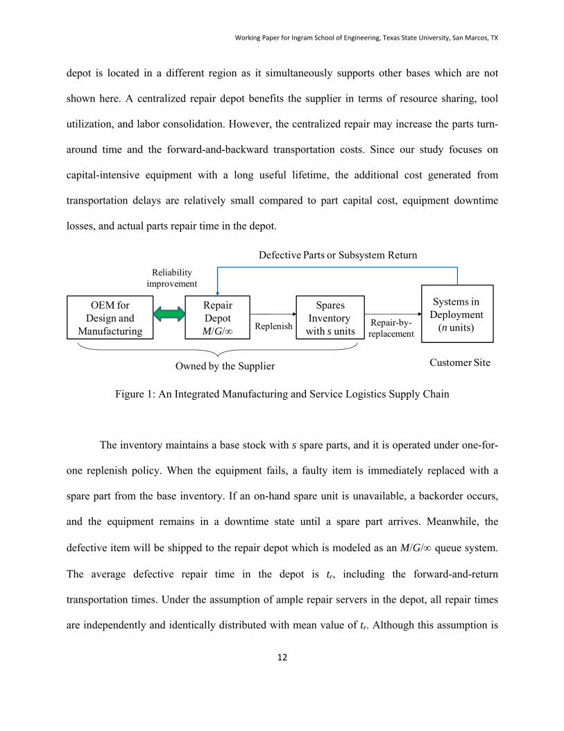
Working Paper for Ingram School of Engineering, Texas State University, San Marcos, TX
12
depot is located in a different region as it simultaneously supports other bases which are not
shown here. A centralized repair depot benefits the supplier in terms of resource sharing, tool
utilization, and labor consolidation. However, the centralized repair may increase the parts turn-
around time and the forward-and-backward transportation costs. Since our study focuses on
capital-intensive equipment with a long useful lifetime, the additional cost generated from
transportation delays are relatively small compared to part capital cost, equipment downtime
losses, and actual parts repair time in the depot.
SparesInventory
with s units
Systems inDeployment
(n units)
OEM forDesign and
ManufacturingRepair-by-replacement
RepairDepotM/G/ Replenish
Defective Parts or Subsystem Return
Reliabilityimprovement
Owned by the Supplier Customer Site
Figure 1: An Integrated Manufacturing and Service Logistics Supply Chain
The inventory maintains a base stock with s spare parts, and it is operated under one-for-
one replenish policy. When the equipment fails, a faulty item is immediately replaced with a
spare part from the base inventory. If an on-hand spare unit is unavailable, a backorder occurs,
and the equipment remains in a downtime state until a spare part arrives. Meanwhile, the
defective item will be shipped to the repair depot which is modeled as an M/G/ queue system.
The average defective repair time in the depot is tr, including the forward-and-return
transportation times. Under the assumption of ample repair servers in the depot, all repair times
are independently and identically distributed with mean value of tr. Although this assumption is
Working Paper for Ingram School of Engineering, Texas State University, San Marcos, TX
13
quite ideal, Sherbrooke (1992) shows that this is a reasonable approximation in many repairable
inventory circumstances.
Two scenarios will occur at the customer site upon the occurrence of system failures. If a
spare part is available in the local stock, the repair-by-replacement job can be performed
immediately. The average time used for performing this replacement job is denoted as ts. If an
on-hand spare item is not available, the repair-by-replacement job cannot be executed until the
arrival of the spare part. In this case, the equipment downtime, hence the MTTR, is prolonged
due to the waiting time for the spare unit. In the following, we will derive the MTTR model
taking both scenarios into consideration.
Two important random variables are on-hand inventory Q and backorder B, which have a
substantial impact on the MTTR. Assuming the supplier sets the base stocking level as s units,
then Q and s are related with each other through Q=max{0, s-O}, where O is a random variable
representing the steady-state inventory on-order. Similarly, B and s are related with each other
through B=max{0, O-s}. According to Palm’s Theorem, O can be modeled as a Poisson
distribution with mean o=natr. Notice that na is the aggregate fleet failure rate, and tr is the
average repair turn-around time for a defective unit. The assumption for a fixed fleet failure rate,
i.e. na, is in fact an approximation, because the field-repair loop with a finite installed base
means o depends on the number of actual working systems in the field. This approximation is
reasonable in our analysis because the condition o<<n usually is satisfied in practical
applications. If dT denotes the MTTR, then we have
}Pr{1)(}Pr{ sOttsOtT rssd (5)
Where
Working Paper for Ingram School of Engineering, Texas State University, San Marcos, TX
14
s
x
xo
x
esO
0 !}Pr{
0
, and o=natr (6)
Here x is the number of spare parts in demand. Equations (5) provides an analytical
insight into the interrelationship between the MTTR and the key performance drivers such as ts,
tr, s, a, and n. It allows us to control or reduce the MTTR by tuning one or several parameters
depending on the available resources. Notice that ts is the time for performing the repair-by-
replacement job given the on-hand spare part is available. In cases that ts<<tr or Pr{Os}0,
equation (5) can be further simplified as dT =trPr{O>s}, which becomes the same MTTR model
given by Kim et al. (Kim et al. 2007). Finally, equations (7) and (8) below allow us to compute
the expected values for Q and B, respectively
s
x
xo
x
exsQE
o
0 !)(][ (7)
s
x
xo
o x
esxsBE
o
0 !)(][
s
x
tnxr
r x
etnsxstn
r
0 !)(
(8)
Similar to the MTTR, both the on-hand and the backorder quantities depend on the key
performance drivers: product inherent failure rate, the base stock level, the usage rate, the repair
turn-around time, and the size of installed base.
3.3. Equipment Availability-A New Perspective
As discussed previously, equipment time can be broken down into three categories:
operating time, standby time, and down time. Let oT , sT and dT be the expected value for each of
these, then the operational availability can be defined as
Working Paper for Ingram School of Engineering, Texas State University, San Marcos, TX
15
do
o
dso
soo TT
T
TTT
TTA
/
/ (9)
Notice that is the usage rate defined in equation (4). Incorporating the usage rate into
the availability model is an important step to reach a win-win contractual agreement between the
customer and the service provider. Compared with equation (1), the model in equation (8) is a
more realistic metric to assess the equipment availability as it takes the consideration of the
usage uncertainty. OEM can make every effort to reduce the product inherent failure rate, hence
increase the operational availability, through re-designs and adoption of new materials or
technologies. The usage rate will assist OEM and the equipment users in reaching a realistic
availability goal which might be different under different utilizations such as regular trainings
and military engagements. Finally, by substituting equations (3), (5) and (6) into (9), the
availability can be expressed as
s
x
tnxr
rs
ro
x
etntt
tnsAr
0 !
)(11
1),,,,( (10)
Up to now, we have analytically developed a new availability model that draws upon two
distinct bodies of literature. We applied the classical repairable inventory theory to estimate
equipment MTTR. This metric is further evolved into a novel availability model, Ao, which has
not been previously reported in literature. The new model elegantly brings together all key
performance drivers, i.e. , s, , n, and tr, under a unified framework. By introducing this new
assessment instrument, which has always been surrogated simply by the availability of spare
parts, we have established the theoretical foundation for the operation and management of
performance based service contracts.
3.4. Fleet Readiness
Working Paper for Ingram School of Engineering, Texas State University, San Marcos, TX
16
Assuming the fleet consists of n identical systems for which their annual usage rate is
similar. Then the fleet readiness is defined as the probability that there are at least k systems
available at any random point in time. This can be expressed analytically as
n
ki
ini AAi
nkN )1(}Pr{ , for k=0, 1, …, n (11)
Where, N is a random variable representing the number of available systems, and k is a
predetermined integer value by the customer. For example, if A=0.95, n=20, and k=18, then
Pr{N18}=0.925. This implies, with probability 0.925, there are at least 18 systems in the fleet
are ready for operation at any time upon the mission request. Methodologically, the fleet
readiness is not new and it is simply a type of quantile estimate. But from the military point of
view, it is often more concerned with the probability that enough aircrafts can fly for a particular
mission, instead of the average number of mission capable aircrafts (Kang and McDonald 2010).
4. Lifecycle Cost Analysis
The new availability model in equation (10) shows that equipment availability is
determined by multiple factors: the inherent reliability , base stocking level s, defective repair
time tr, usage rate β, and the size of the installed base n. Hence, cost analysis for PBL contracting
must be approached and analyzed from the product lifecycle perspective. Besides the spare parts
inventory, cost factors associated with the design and manufacturing need to be assessed and
incorporated into the decision model when one constructs the PBC policy. Without loss of
generality, the following cost models are developed for one particular part type or LRU. The
lifecycle cost for the system can be calculated by aggregating the cost of individual part types.
4.1. Design Cost versus Reliability
Working Paper for Ingram School of Engineering, Texas State University, San Marcos, TX
17
Although it is widely agreed that the product design cost increases with the growth of
reliability, the consensus on how to describe such a relationship is still not reached in literature.
Many studies such as (Mettas 2000, Yeh and Lin 2009) show that the design cost in general
grows exponentially as reliability increases. Let D() be the design cost for the product with a
failure rate of , then the exponential design cost model can be expressed as
min
max1 exp)(
BD , for minmax (12)
Where, max and min represent the maximum and the minimum product failure rates,
respectively. Quite often, 1/max is the minimum MTBF per the customer requirement, and 1/min
is the best achievable MTBF by the OEM. Notice that B1 and are positive parameters. In
particular, B1 is the baseline design cost for the product with max, and characterizes the
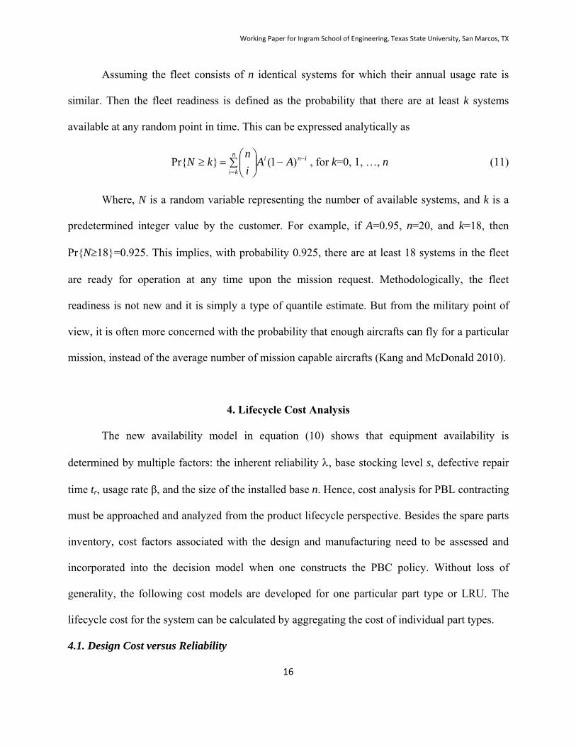
difficulties in reducing the failure rate under materials and resource constraints. Figure 2 depicts
two design-reliability cost functions for =0.02 and 0.05, respectively. Both examples show that
design cost will rapidly increase once the reliability reaches a certain level.
1.0
1.2
1.4
1.6
1.8
2.0
20000 24000 28000 32000 36000 40000
Cos
t ($)
Design Cost vs. Reliability
(10
6 ) B1=1106
=0.05
=0.02
1/
Figure 2: Product Design Cost vs. Reliability
Working Paper for Ingram School of Engineering, Texas State University, San Marcos, TX
18
4.2. Manufacturing Cost versus Reliability
Producing a highly reliable product requires adoption of new materials, improved
technology and advanced manufacturing processes. As a result, the manufacturing cost increases
with the reliability. Let c() represent the manufacturing cost per unit item, then the cost can be
estimated as
max
32
11)( BBc , for minmax (13)
Equation (13) is a modified version of the manufacturing cost model originally proposed
by Öner et al. (2010). We assume the design cycle is relatively short compared to the product
useful lifetime. Hence the learning effects can be ignored in the cost model. For production cost
models considering learning effects, readers are referred to Huang et al. (2007) and Loerch
(1999). In equation (13), B2 is the baseline unit production cost with failure rate of max.
Parameters B3 and capture the incremental cost when is further reduced relative to max. All
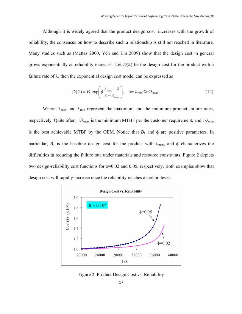
model parameters are positive numbers. Figure 3 presents three manufacturing cost models under
B2=$105 and B3=$2,000 with =0.4, 0.5, and 0.6, respectively. Given the same B2 and B3, a
higher production cost will be incurred if is larger.
Working Paper for Ingram School of Engineering, Texas State University, San Marcos, TX
19
0
100,000
200,000
300,000
400,000
500,000
600,000
20,000 25,000 30,000 35,000 40,000
Cos
t($)
Manufacturing Cost vs. Reliability
B2=1105
B3=2,000
1/
=0.6
=0.5
=0.4
Figure 3: Product Manufacturing Cost vs. Reliability
4.3. Service Logistics Cost
The service logistics expenditures consist of the inventory cost and the repair cost. The
major portion of the inventory is the investment on spare parts. The repair costs include the part
transportation fees, the labor cost, and repair facilities. Let I(, β, s, n) be the service logistics
cost incurred in the contractual period of years, then
),()(),,,( ncscnsI r (14)
Where
)1(
1)1(),(
(15)
In equation (14), the first term represents the one-time base stock capital investment, and
the second component represents the present value of total repair costs incurred during [0, ].
Notice that cr is the repair cost per defective item. It includes the costs associated with labors,
repair facility, part shipment between repair depot and the base. (, ) is the coefficient to
Working Paper for Ingram School of Engineering, Texas State University, San Marcos, TX
20
calculate the present value of annuity with the annual interest rate . Since military PBL
contracts often involve long-term service commitment, minimizing the lifecycle cost must take
into account the effects of money in time.
4.4. System Lifecycle Cost
For the supplier, the lifecycle cost consists of the product design cost, manufacturing cost,
and after-sales service logistics cost. Let π(, β, s, n) denote the lifecycle cost for n working units
deployed in the customer site. Then the lifecycle cost for the n-unit fleet is given as
),,,()()(),,,( nsIncDns (16)
5. Optimization for Performance Based Logistics
After the lifecycle cost model is derived, the next step for the customer is to develop the
contractual payment plan. Although PBL as a logistic support strategy has been used for about
ten years, there are few quantitative processes and procedures that are mature and available to
guide suppliers to achieve the performance goal through optimal resource allocation. Under the
PBC scheme, the service supplier will be rewarded monetarily if the equipment availability is
sustained above a threshold or Amin as defined by the customer. Depending on the rewarding
methods, two options can be chosen by the service provider: cost minimization or profit
maximization.
5.1. Lifecycle Cost Minimization
Cost minimization strategy is preferred if the system design is relatively new and few
reliability data are available. In that case, the customer prefers to control the after-sales service
payment bill as well as to mitigate the uncertainty in equipment availability. The supplier, on the
other hand, may choose to minimize the total lifecycle cost of the product while meeting the
Working Paper for Ingram School of Engineering, Texas State University, San Marcos, TX
21
availability criterion. The following optimization model, denoted as Problem P1, is formulated to
minimize the product lifecycle cost
Problem P1:
Min );,()()();,( sIncDs (17)
Subject to
A(, s; β)Amin (18)
minmax (19)
Problem P1 is formulated to determine the optimal and s such that the lifecycle cost of
the fleet equipment is minimized for a period of years. A(, s; β), D(), c(), and I(, s; β) are
given in equations (10) and (12)-(14), respectively. Notice that constraint (18) ensures the
availability being always higher than Amin. Equation (19) specifies the product inherent failure
rate must fall into the range between min and max.
As shown in Equation (4), β has a significant impact on the actual equipment failure rate.
It is a random variable which may vary over the planning horizon. For instance, heavier usages
are often observed for military aircraft during mission engagement period compared to regular
training seasons. In power industry, the utilization rate of power generation equipment also
varies from hour to hour, day to day, and season to season due to the demand variability. Hence
P1 actually is a stochastic programming model due to the random nature of . Stochastic
programming problems can be solved by using simulation-based approaches or converting it into
a deterministic model. Simulation approach randomly generates a usage scenario, each of which
will be solved in a deterministic fashion. The final result is obtained by taking the average of the
entire solution set. The result obtained from the simulation-based approach is quite accurate, but
Working Paper for Ingram School of Engineering, Texas State University, San Marcos, TX
22
the computational cost and time could be large as well. To solve Problem P1 in a reasonable
computational time, we transform the original problem into a deterministic model, denoted as P2,
by taking the expectation with respect to as following
Problem P2:
Min );,()()()];,([ sIncDsE (20)
Subject to
E[A(, s; β)]Amin (21)
minmax (22)
Where, =E[] is the mean value of . It is still difficult to compute E[A(, s; β)] due to
the analytical complexity in A(, s; β). To make P2 mathematically tractable, yet without
compromising the accuracy, A(, s; ) will be used as an approximation for E[A(, s; β)]. Now
the problem is to find the optimal and s such that the expected lifecycle cost is minimized
while the availability criterion is still satisfied.
5.2. Profit-centric Maximization
Since PBL incentives are now designed to reward high operational reliability and
availability of equipment, suppliers will naturally shift their concentration from purely cost
reduction to profit maximization. We are going to integrate revenue function into the service
decision-making model and to show how this will affect the resource allocation. We adopt the
linear and the exponential models originally proposed by Nowicki et al. (2008) to allocate
resources such that the supplier’s profit margin will be maximized. The linear and the
exponential revenue functions are restated as follows
Working Paper for Ingram School of Engineering, Texas State University, San Marcos, TX
23
min
minmin
0
)()(
AA
AAAAbaAR (23)
min
minmin
0
)(exp)(
AA
AAAAAR
(24)
Both (a, b) and (, ) are parameters for the linear and exponential models, respectively.
Different shapes of revenue functions can be obtained by tuning the model parameters. For
instance, a larger b or implies the supplier will reap more financial benefits as A increases.
Assuming a system is configured with K types of subsystems for i=1, 2, …, K. Each type
of subsystem might be duplicated in the system due to the functional requirement. This
duplicated configuration is quite common in repairable systems. For instance, a wind turbine has
multiple DC/AC converters of the same type. Based on equations (23) and (24), the following
profit maximization model for a fleet of systems, denoted as P3, is formulated
Problem P3:
Max
K
iiii
K
iiiii
K
iiiis sIBcmnBDARsPE
11,2
1,1 );,()()());,(()];,([ sλ (25)
Subject to
min,iimax,i for i=1,2, …., K (26)
min1
;,();,( AsAAimK
iiiis
sλ (27)
Where, );,( sλsA is defined as the system-level availability given the availability of
individual subsystems. mi is the number of subsystem type i used in the system, and K is the
number of subsystem types. The profit-centric model is formulated to determine the optimal i
and si for subsystem type i such that the profit margin for maintaining the entire fleet is
Working Paper for Ingram School of Engineering, Texas State University, San Marcos, TX
24
maximized. The objective function in equation (25) is designed to motivate the supplier to
improve the product reliability through re-design or adoption of advanced manufacturing
technology after the product shipment. Therefore costs for baseline design (i.e. B1) and
manufacturing (i.e. B2) are excluded from the objective function. Numerical example will be
provided in Section 6 to demonstrate the application of this model.
5.3. Solution Algorithms
Problems P2 and P3 belong to non-linear mixed integer programming problems. These
types of problems are in general difficult to solve because they involve the complexity of
nonlinearity and the combinatorial natures of integer programs (Gupta and Ravindran 1985).
Existing algorithms generally rely on the successive solutions of closely related non-linear
programming problems, and then the branch-and-bound technique to explore the integer solution.
Recently, genetic algorithm and heuristic methods (Coit et al. 2004, Marseguerra et al. 2005)
have shown to be effective in searching for the optimal or near optimal solution for complex
non-linear programming problems within a reasonable computation time.
Since Problem P2 only involves two variables and s, we can use the iteration method to
find the optimal solution. The detailed procedure is given as follows: starting with s=0, we let
increase from min and max by a small step and compute the objective function. Then we
increasing s=s+1 and repeat the same process. If the current cost is lower than the previous
interaction, choose the current s and as the optimal solution, otherwise a new iteration begins
by increase s=s+1. The process is repeated until s reaches a reasonable level, then we stop the
iteration. The iteration method cannot be applied to Problem P3 because the number of the
decision variables is relatively large (K>>2). Therefore, we will develop a genetic algorithm to
search the optimal values of i and si for i=1,2, …, K.
Working Paper for Ingram School of Engineering, Texas State University, San Marcos, TX
25
6. Numerical Examples
Two examples drawn from the military sector and the semiconductor industry will be
used to demonstrate the PBL contracting program discussed in this paper. The first example aims
to find the optimal resource allocation to product development and after-sales services such that
the reliability performance of aircraft’s avionics subsystems is warranted. The supplier’s
objective is to minimize the subsystem lifecycle cost by taking account of design, manufacturing,
and spare parts inventory. The second example is chosen from the semiconductor manufacturing
industry where equipment useful lifetime is relatively short due to the technological
obsolescence. As such the goal for the OEM is to maximize the service profit margin while
meeting the customer’s reliability goal.
6.1. PBL Contracting for Subsystems
In this example, the OEM is contracted to design and supply high-end avionics
subsystems to the military customers. With some slight modifications, we use the avionics cost
data originally given in (Kim et al. 2007) to construct the numerical example. Table 1 presents
the necessary information for carrying out the cost analysis based on the optimization model in
Problem P2. We assume the baseline manufacturing cost is B1=$25,000 per subsystem. The
maximum acceptable failure rate by the customer is max=1.752 faults/year, and the best
achievable failure rate by the OEM is min=0.876 faults/year. These values are selected based on
the field analysis of avionics reliability in (Moreno 1990). We further assume ts=0.1tr, meaning
the time to replace a defective subsystem is only 10% of tr when the spare part is available at the
customer site. All other parameters are self-explained.
Working Paper for Ingram School of Engineering, Texas State University, San Marcos, TX
26
Table 1: Parameters for Avionics Subsystems
Parameter Value Parameter Value
0.05 B1 ($) 500,000
0.02 B2 ($) 25,000
max (faults/year) 1.752 B3 ($) 2,000
min (faults/year) 0.876 0.6
cr ($/part) 5,000 ts (days) 0.1tr
Our purpose is to help OEM analyze various contractual scenarios and make the best
decision on and s such that the LCC (lifecycle cost) is minimized. Other variables that need to
be considered include the minimum availability threshold Amin, the fleet size n, the repair turn-
around time tr, and the usage rate β. It is worth mentioning that β usually involve large
uncertainties due to the stochastic nature of military operations and engagements. Therefore, two
usage rates, i.e. β=0.5 and 0.75, are used to calculate the anticipated LCC, and the results will be
compared in terms of spare parts provisioning levels.
Table 2: LCC Minimization for =5 years and Amin=0.95
usage rate =0.5 =0.75
fleet size n=200 n=500 n=200 n=500
repair time (days) tr=30 tr=60 tr=30 tr=60 tr=30 tr=60 tr=30 tr=60
(faults/year) 0.9505 0.9373 0.9286 0.9242 0.9329 0.9286 0.9198 0.9198
s 0 14 0 36 8 24 23 59
A 0.959 0.951 0.960 0.951 0.950 0.950 0.951 0.952
LCC ($106) 7.80 8.17 18.54 19.46 9.03 9.45 21.63 22.55
LCC/year ($106) 1.56 1.63 3.71 3.89 1.81 1.89 4.33 4.51
Working Paper for Ingram School of Engineering, Texas State University, San Marcos, TX
27
Table 2 summarizes the optimal values for and s under a 5-year service agreement. A
general conclusion is that deceases and s increases when β, n, or tr becomes larger in order to
meet Amin. It is interesting to see that spare parts are not needed when β=0.5 and tr=30 days. In
fact there is no surprise to obtain this conclusion after we re-examine the availability metric in
Equation (9). It clearly shows that a high A(, s; β) can be attained by reducing , β, or tr, instead
of increasing s. The table also shows that s is highly correlated with β and tr. For instance, when
β=0.5, n=500 and tr=60 day, at least 36 spare parts are required at the base inventory to support
the minimum availability as opposed to s=0 if tr=30 days. Finally the optimal failure rate
decreases as n becomes large.
Table 3: LCC Minimization for =15 years and Amin=0.95
usage rate =0.5 =0.75
fleet size n=200 n=500 n=200 n=500
repair time (days) tr=30 tr=60 tr=30 tr=60 tr=30 tr=60 tr=30 tr=60
(faults/year) 0.9242 0.9242 0.9110 0.9067 0.9198 0.9198 0.9023 0.9067
s 0 14 0 35 8 24 22 58
A 0.960 0.953 0.960 0.950 0.952 0.952 0.950 0.951
LCC ($106) 10.64 10.99 25.47 26.38 13.23 13.64 31.93 32.85
LCC/year ($106) 0.709 0.733 1.698 1.758 0.882 0.910 2.13 2.19
Table 3 presents the optimal values for and s under a 15-year service agreement with
Amin=0.95. Two distinctive observations can be made by comparing to Table 2. The annualize
LCC for the long-term contract is less than 50% of the cost in the 5-year contract. This is
because the design and manufacturing costs are absorbed in a longer period, making the yearly
cost distribution lower than that in a short-term contract. Another observation is that a lower is
Working Paper for Ingram School of Engineering, Texas State University, San Marcos, TX
28
more favorable to the OEM for a 15-year contract. In other words, OEM is willing to invest more
resources on design and manufacturing under a long-term PBL contract. It is also observed that
the contractual length has smaller impact on the level of the spare parts inventory.
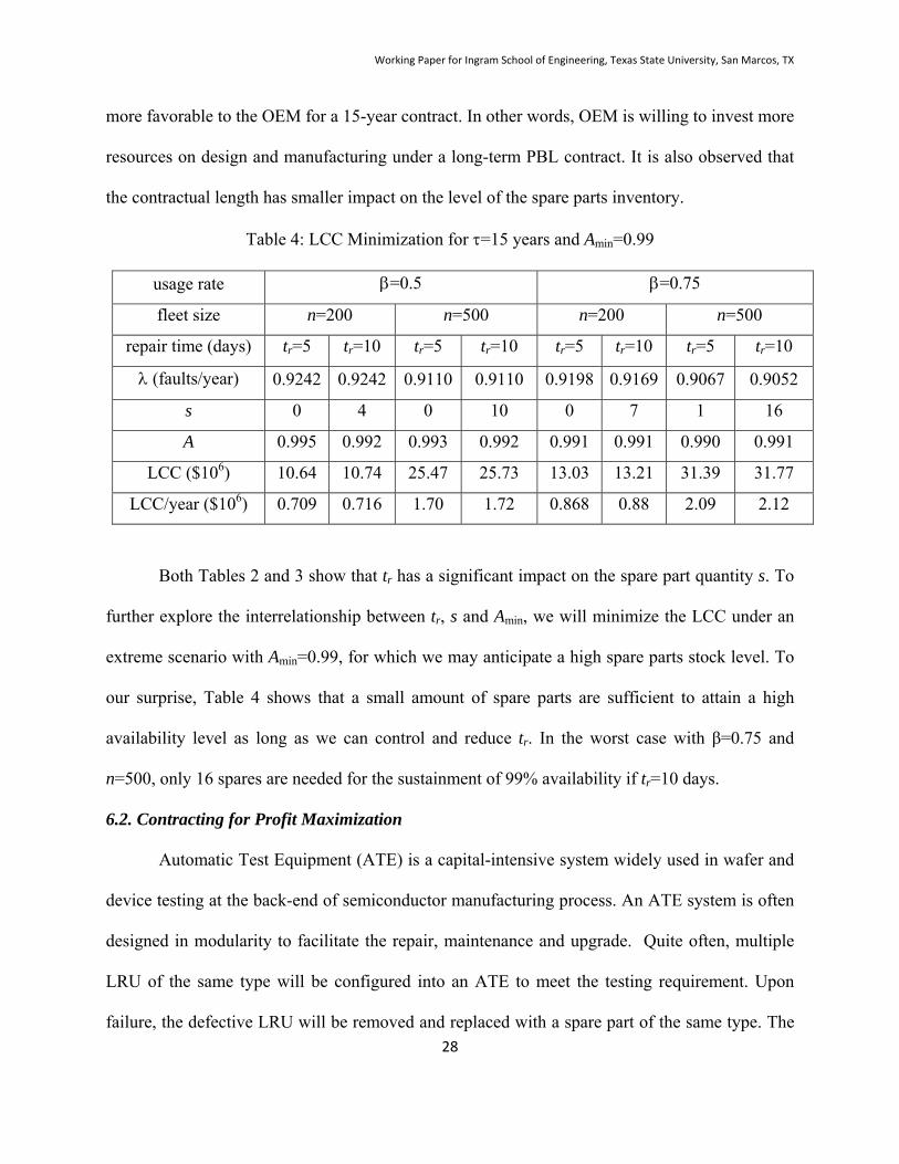
Table 4: LCC Minimization for =15 years and Amin=0.99
usage rate =0.5 =0.75
fleet size n=200 n=500 n=200 n=500
repair time (days) tr=5 tr=10 tr=5 tr=10 tr=5 tr=10 tr=5 tr=10
(faults/year) 0.9242 0.9242 0.9110 0.9110 0.9198 0.9169 0.9067 0.9052
s 0 4 0 10 0 7 1 16
A 0.995 0.992 0.993 0.992 0.991 0.991 0.990 0.991
LCC ($106) 10.64 10.74 25.47 25.73 13.03 13.21 31.39 31.77
LCC/year ($106) 0.709 0.716 1.70 1.72 0.868 0.88 2.09 2.12
Both Tables 2 and 3 show that tr has a significant impact on the spare part quantity s. To
further explore the interrelationship between tr, s and Amin, we will minimize the LCC under an
extreme scenario with Amin=0.99, for which we may anticipate a high spare parts stock level. To
our surprise, Table 4 shows that a small amount of spare parts are sufficient to attain a high
availability level as long as we can control and reduce tr. In the worst case with β=0.75 and
n=500, only 16 spares are needed for the sustainment of 99% availability if tr=10 days.
6.2. Contracting for Profit Maximization
Automatic Test Equipment (ATE) is a capital-intensive system widely used in wafer and
device testing at the back-end of semiconductor manufacturing process. An ATE system is often
designed in modularity to facilitate the repair, maintenance and upgrade. Quite often, multiple
LRU of the same type will be configured into an ATE to meet the testing requirement. Upon
failure, the defective LRU will be removed and replaced with a spare part of the same type. The
Working Paper for Ingram School of Engineering, Texas State University, San Marcos, TX
29
defective part is then sent to the depot for repair. After repair, it becomes ready-for-use and will
be sent back to the local spare pool.
PBL contracts will be investigated in terms of LRU shipping volume and unit cost in
three different categories: 1) low volume and low cost (LVLC); 2) high volume and low cost
(HVLC); and 3) low volume and high cost (LVHC). These categories represent the typical
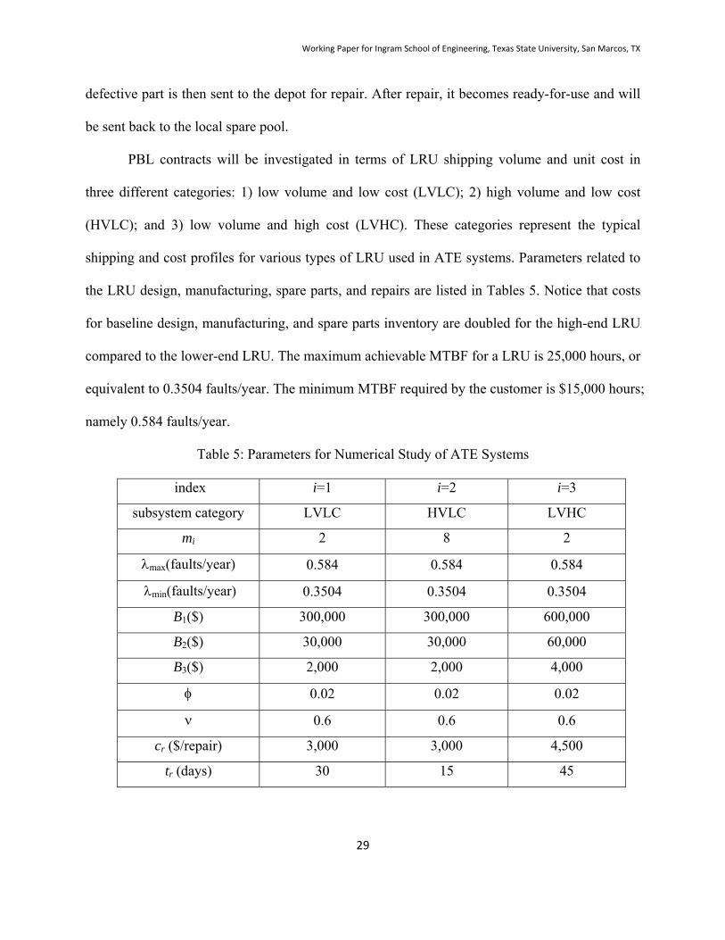
shipping and cost profiles for various types of LRU used in ATE systems. Parameters related to
the LRU design, manufacturing, spare parts, and repairs are listed in Tables 5. Notice that costs
for baseline design, manufacturing, and spare parts inventory are doubled for the high-end LRU
compared to the lower-end LRU. The maximum achievable MTBF for a LRU is 25,000 hours, or
equivalent to 0.3504 faults/year. The minimum MTBF required by the customer is $15,000 hours;
namely 0.584 faults/year.
Table 5: Parameters for Numerical Study of ATE Systems
index i=1 i=2 i=3
subsystem category LVLC HVLC LVHC
mi 2 8 2
max(faults/year) 0.584 0.584 0.584
min(faults/year) 0.3504 0.3504 0.3504
B1($) 300,000 300,000 600,000
B2($) 30,000 30,000 60,000
B3($) 2,000 2,000 4,000
0.02 0.02 0.02
0.6 0.6 0.6
cr ($/repair) 3,000 3,000 4,500
tr (days) 30 15 45
Working Paper for Ingram School of Engineering, Texas State University, San Marcos, TX
30
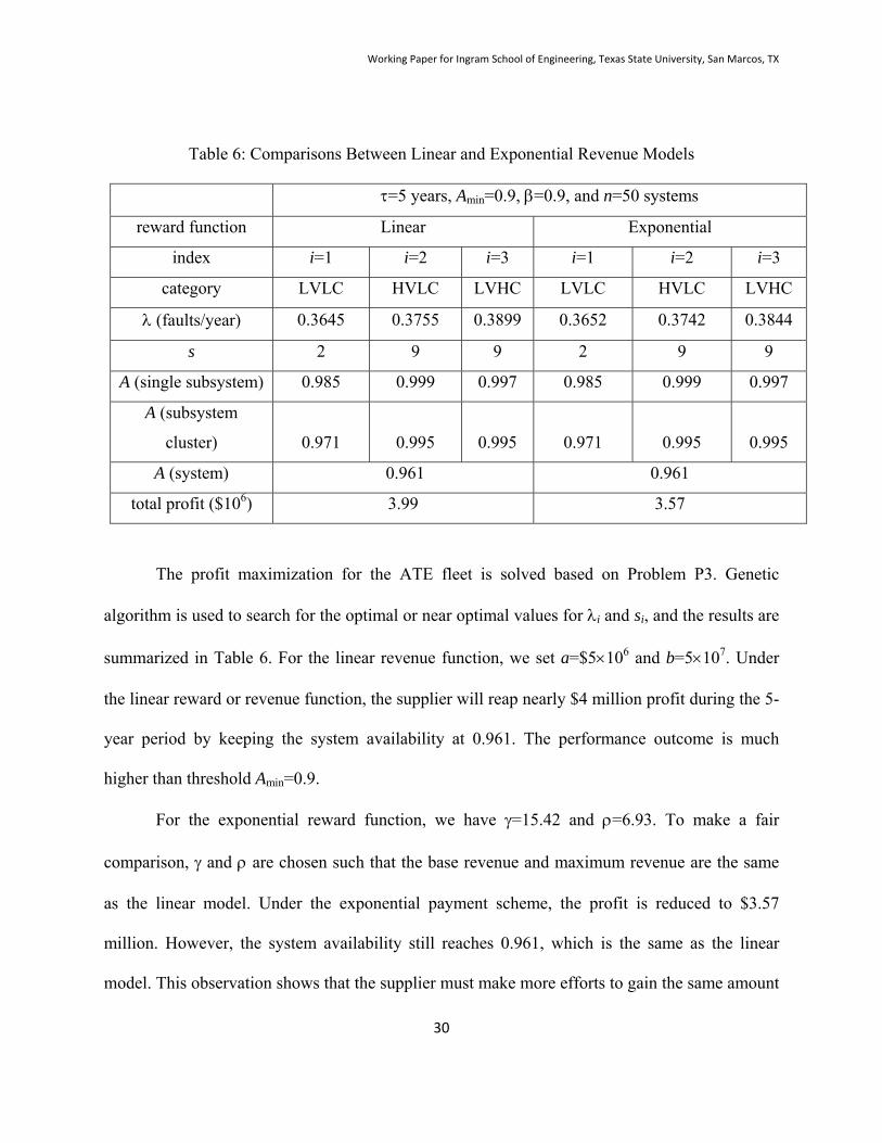
Table 6: Comparisons Between Linear and Exponential Revenue Models
=5 years, Amin=0.9, =0.9, and n=50 systems
reward function Linear Exponential
index i=1 i=2 i=3 i=1 i=2 i=3
category LVLC HVLC LVHC LVLC HVLC LVHC
(faults/year) 0.3645 0.3755 0.3899 0.3652 0.3742 0.3844
s 2 9 9 2 9 9
A (single subsystem) 0.985 0.999 0.997 0.985 0.999 0.997
A (subsystem
cluster) 0.971 0.995 0.995 0.971 0.995 0.995
A (system) 0.961 0.961
total profit ($106) 3.99 3.57
The profit maximization for the ATE fleet is solved based on Problem P3. Genetic
algorithm is used to search for the optimal or near optimal values for i and si, and the results are
summarized in Table 6. For the linear revenue function, we set a=$5106 and b=5107. Under
the linear reward or revenue function, the supplier will reap nearly $4 million profit during the 5-
year period by keeping the system availability at 0.961. The performance outcome is much
higher than threshold Amin=0.9.
For the exponential reward function, we have =15.42 and =6.93. To make a fair
comparison, and are chosen such that the base revenue and maximum revenue are the same
as the linear model. Under the exponential payment scheme, the profit is reduced to $3.57
million. However, the system availability still reaches 0.961, which is the same as the linear
model. This observation shows that the supplier must make more efforts to gain the same amount
Working Paper for Ingram School of Engineering, Texas State University, San Marcos, TX
31
of the profit under the exponential reward function. This in fact gives customer the advantage for
designing the contractual payment plan while reducing the cost ownership. The inventory
decision on both cases happened to be the same. Both HVLC and LVHC require a high stocking
level either because of high volume shipment for HVLC or the repair turn-around time is long
for LVHC.
7. Conclusion
We have proposed a general model comprehending the equipment availability in the light
of several key performance drivers including product reliability, usage uncertainty, spares parts
inventory, repair turn-around time, and the installed base. Under the PBC scheme, two
optimization models are investigated in the context of minimizing the lifecycle cost or
maximizing the service profit. Our study shows that reliability investment should be made early
in the product lifecycle in order to reduce the total cost of ownership. The second observation is
that quick repair turn-around time can significantly reduce the base stock level, hence increase
the equipment availability. The study shows that PBL contracts must be constructed to meet the
equipment availability threshold as well as the reliability goal. The latter one is often referred as
MTBF or the inherent product failure rate. Although the equipment availability could be
sustained by relying on a large spare items pool, this approach is not financially attractive to the
supplier due to the excessive inventory cost. Meanwhile the customer is also dissatisfied with the
excessive downtime failures. PBC provides lower overall sustainment costs for the equipment
users, and profit growth opportunity for the service contractors. The supplier is incentivized to
invest resources wisely across the design, manufacturing, and spare parts logistics such that the
lifecycle cost is minimized. The availability model developed for two-echelon repairable
Working Paper for Ingram School of Engineering, Texas State University, San Marcos, TX
32
inventory can be expanded and incorporate more realistic conditions such as dynamic installed
base, reliability growth planning, and lateral resupply. These are the potential areas we would
like to concentrate on in the future.
References
[1] Axsäter, S. 1990. Modelling emergency lateral transshipments in inventory systems.
Management Science. vol. 36, no. 11, pp. 1329-1338.
[2] Coit, D.W., T. Jin, N. Wattanapongsakorn. 2004. System optimization considering
component reliability estimation uncertainty: multi-criteria approach. IEEE Transactions
on Reliability, vol. 53, no.3, pp. 369-380.
[3] Elsayed, E.A.1996. Reliability Engineering, Chapter 9, Addison Wesley Longman
Publisher.
[4] Gadiesh, O., J.L. Gilbert. 1998. Profit pools: a fresh look at strategy. Harvard Business
Review, vol. 76, no. 3, pp. 139-147.
[5] Graves, S.C. 1985. A multi-echelon inventory model for a repairable item with one-for-one
replenishment. Management Science, vol. 31, no. 10, pp. 1247-1256.
[6] Gupta, O.K., A. Ravindran. 1985. Branch and bound experiments in convex nonlinear
integer programming. Management Science, vol. 31, no. 12, pp. 1533-1546.
[7] Huang, H.-Z., H.J. Liu, D.N.P. Murthy. 2007. Optimal reliability, warranty and price for
new products. IIE Transactions, vol. 39, no. 8, pp. 819-827.
[8] Kang, K., M. McDonald. 2010. Impact of logistics on readiness and life cycle cost: a
design of experiments approach, Proceedings of Winter Simulation Conference. pp. 1336-
1346.
Working Paper for Ingram School of Engineering, Texas State University, San Marcos, TX
33
[9] Kennedy, W.J., J.W. Patterson, L.D. Fredenhall. 2002. An overview of recent literature on
spare parts inventories. International Journal of Production Economics, vol. 76, no. 2, pp.
210-215.
[10] Kim, S.H., M.A. Cohen, S. Netessine. 2007. Performance contracting in after-sales service
supply chains. Management Science, vol. 53, pp. 1843-1858.
[11] Kim, S.H., M.A. Cohen, S. Netessine. 2010. Reliability or inventory? analysis of product
support contracts in the defense industry. Working Paper, Yale University.
[12] Kuo, W., R. Wan. 2007. Recent advances in optimal reliability allocation. IEEE
Transactions on Systems, Man, and Cybernetics, vol. 37, no. 2, pp. 143-156.
[13] Jin, T., H. Liao. 2009. Spare parts inventory control considering stochastic growth of an
installed base. Computers & Industrial Engineering, vol. 56, no. 1, pp. 452-460.
[14] Lee, H.L. 1987. A multi-echelon inventory model for repairable items with emergency
lateral transshipments. Management Science, vol. 33, no. 10, pp. 1302-1316.
[15] Loerch, A.G. 1999. Incorporating learning curve costs in acquisition strategy optimization.
Naval Research Logistics. vol. 46, pp. 255–271.
[16] Marseguerra, M., E. Zio, L. Podofillini. 2005. Multi-objective spare parts allocation by
means of genetic algorithms and Monte Carlo simulations. Reliability Engineering and
System Safety, vol. 87, no. 3, pp. 325-335.
[17] Mettas, A. 2000. Reliability allocation and optimization for complex systems. Proceedings
of Reliability and Maintainability Symposium, pp. 216-221.
[18] Moreno, F.J. 1999. MTBF warranty/guarantee for multiple user avionics. Proceedings of
Annual Reliability and Maintainability Symposium. pp. 113-119.
Working Paper for Ingram School of Engineering, Texas State University, San Marcos, TX
34
[19] Muckstadt, J. A. 2005. Analysis and Algorithms for Service Parts Supply Chains. Springer,
New York.
[20] Nowicki, D., U.D. Kumar, H.J. Steudel, D. Verma. 2008. Spares provisioning under
performance-based logistics contract: profit-centric approach. The Journal of the
Operational Research Society. vol. 59, no. 3, 2008, pp. 342-352.
[21] Oliva, R., R. Kallenberg. 2003. Managing the transition from products to services.
International Journal of Service Industry Management. vol. 14, no. 2, pp.160-172.
[22] Öner, K.B., G.P. Kiesmüller, G.J. van Houtum. 2010. Optimization of component
reliability in the design phase of capital goods. European Journal of Operational Research,
vol. 205, no. 3, pp. 615-624.
[23] Richardson, D., A. Jacopino. 2006. Use of r&m measures in Australian defense aerospace
performance based contracts. Proceedings of Reliability and Maintainability Symposium,
pp. 331-336.
[24] Sherbrooke, C.C. 1968. METRIC: A multi-echelon technique for recoverable item control.
Operations Research. vol. 16, no. 1, pp. 122-141.
[25] Sherbrooke, C.C. 1992. Multiechelon inventory systems with lateral supply. Naval
Research Logistics. vol. 39, pp. 29-40.
[26] Telcordia Technologies. 2001. Special Report SR-332: Reliability Prediction Procedure for
Electronic Equipment (Issue 1). Telcordia Customer Service, Piscataway, New Jersey.
[27] U.S. Department of Defense. 2005. DoD guide for achieving reliability, availability, and
maintainability. U.S. Department of Defense, Washington, D.C.,
http://www.dote.osd.mil/reports/RAMGuide.pdf.
Working Paper for Ingram School of Engineering, Texas State University, San Marcos, TX
35
[28] Wise, R., P. Baumgartner. 1999. Go downstream: the new imperative in manufacturing.
Harvard Business Review, vol. 77, no. 5, 1999, pp. 133-141.
[29] Wong, H., G.J. van Houtum, D. Cattrysse, D. van Oudheusden. 2006. Multi-item spare
parts systems with lateral transshipments and waiting time constraints. European Journal
of Operational Research, vol. 171, no. 3, pp. 1071-1093.
[30] Yeh, W.-C., C.-H. Lin. 2009. A squeeze response surface methodology for finding
symbolic network reliability functions. IEEE Transactions on Reliability, vol. 58, no. 2, pp.
374-382.