Plant functional type mapping for earth system … · Plant functional type mapping for earth system models B. Poulter1,2, P. Ciais2, E. Hodson1, H. Lischke1, ... on the concept of

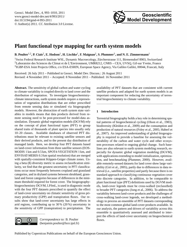
Geosci. Model Dev., 4, 993–1010, 2011www.geosci-model-dev.net/4/993/2011/doi:10.5194/gmd-4-993-2011© Author(s) 2011. CC Attribution 3.0 License.

GeoscientificModel Development

Plant functional type mapping for earth system models

B. Poulter1,2, P. Ciais2, E. Hodson1, H. Lischke1, F. Maignan2, S. Plummer3, and N. E. Zimmermann1

1Swiss Federal Research Institute WSL, Dynamic Macroecology, Zurcherstrasse 111, Birmensdorf 8903, Switzerland2Laboratoire des Sciences du Climat et de L’Environment, UMR8212, CNRS – CEA, UVSQ, Gif-sur Yvette, France3IGBP-ESA Joint Projects Office, c/o ESA-ESRIN, European Space Agency, Via Galileo Galilei, 00044, Frascati, Italy

Received: 26 July 2011 – Published in Geosci. Model Dev. Discuss.: 26 August 2011Revised: 4 November 2011 – Accepted: 8 November 2011 – Published: 16 November 2011

Abstract. The sensitivity of global carbon and water cyclingto climate variability is coupled directly to land cover and thedistribution of vegetation. To investigate biogeochemistry-climate interactions, earth system models require a represen-tation of vegetation distributions that are either prescribedfrom remote sensing data or simulated via biogeographymodels. However, the abstraction of earth system state vari-ables in models means that data products derived from re-mote sensing need to be post-processed for model-data as-similation. Dynamic global vegetation models (DGVM) relyon the concept of plant functional types (PFT) to groupshared traits of thousands of plant species into usually only10–20 classes. Available databases of observed PFT dis-tributions must be relevant to existing satellite sensors andtheir derived products, and to the present day distribution ofmanaged lands. Here, we develop four PFT datasets basedon land-cover information from three satellite sensors (EOS-MODIS 1 km and 0.5 km, SPOT4-VEGETATION 1 km, andENVISAT-MERIS 0.3 km spatial resolution) that are mergedwith spatially-consistent Koppen-Geiger climate zones. Us-ing a beta (ß) diversity metric to assess reclassification simi-larity, we find that the greatest uncertainty in PFT classifica-tions occur most frequently between cropland and grasslandcategories, and in dryland systems between shrubland, grass-land and forest categories because of differences in the mini-mum threshold required for forest cover. The biogeography-biogeochemistry DGVM, LPJmL, is used in diagnostic modewith the four PFT datasets prescribed to quantify the effectof land-cover uncertainty on climatic sensitivity of gross pri-mary productivity (GPP) and transpiration fluxes. Our re-sults show that land-cover uncertainty has large effects inarid regions, contributing up to 30 % (20 %) uncertainty inthe sensitivity of GPP (transpiration) to precipitation. The

Correspondence to:B. Poulter([email protected])

availability of PFT datasets that are consistent with currentsatellite products and adapted for earth system models is animportant component for reducing the uncertainty of terres-trial biogeochemistry to climate variability.

1 Introduction

Terrestrial biogeography holds a key role in determining spa-tial patterns of biogeochemical cycling (Olson et al., 1983),biodiversity (Kleidon et al., 2009) and the consumption andproduction of natural resources (Foley et al., 2005; Haberl etal., 2007). An improved understanding of global biogeogra-phy is required to provide a baseline for assessing the vul-nerability of the carbon and water cycle and other ecosys-tem processes related to ongoing global change. Such base-lines are also relevant to earth system modeling research, es-pecially for dynamic global vegetation modeling (DGVM),with applications extending to model initialization, optimiza-tion, and benchmarking (Plummer, 2000). However, avail-able remotely-sensed datasets for land cover show large vari-ability (Giri et al., 2005), partly due to differences in data re-trieval (i.e., satellite properties) and partly because there is nostandard approach to classifying continuous vegetation coverinto discrete categories. In addition, to be comparable toplant functional type (PFT) definitions used by DGVM mod-els, land-cover legends must be cross-walked (reclassified)to broader PFT categories (Jung et al., 2006). To address thevariability between land-cover products and the challenges ofcross-walking land-cover legends, we developed a method-ology to process an ensemble of PFT datasets correspondingto the most common global land-cover products available. Inour analysis, the pattern and drivers of variability across thisensemble is quantitatively assessed and attributed to inter-pret the effects of land-cover uncertainty on biogeochemicalfluxes.

Published by Copernicus Publications on behalf of the European Geosciences Union.

http://creativecommons.org/licenses/by/3.0/

994 B. Poulter et al.: Plant functional type mapping for earth system models

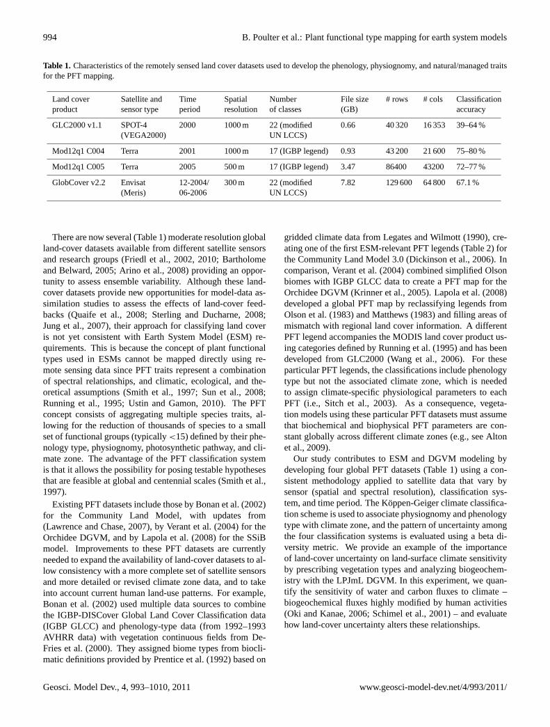
Table 1. Characteristics of the remotely sensed land cover datasets used to develop the phenology, physiognomy, and natural/managed traitsfor the PFT mapping.

Land coverproduct

Satellite andsensor type

Timeperiod

Spatialresolution

Numberof classes

File size(GB)

# rows # cols Classificationaccuracy

GLC2000 v1.1 SPOT-4(VEGA2000)

2000 1000 m 22 (modifiedUN LCCS)

0.66 40 320 16 353 39–64 %

Mod12q1 C004 Terra 2001 1000 m 17 (IGBP legend) 0.93 43 200 21 600 75–80 %

Mod12q1 C005 Terra 2005 500 m 17 (IGBP legend) 3.47 86400 43200 72–77 %

GlobCover v2.2 Envisat(Meris)

12-2004/06-2006

300 m 22 (modifiedUN LCCS)

7.82 129 600 64 800 67.1 %

There are now several (Table 1) moderate resolution globalland-cover datasets available from different satellite sensorsand research groups (Friedl et al., 2002, 2010; Bartholomeand Belward, 2005; Arino et al., 2008) providing an oppor-tunity to assess ensemble variability. Although these land-cover datasets provide new opportunities for model-data as-similation studies to assess the effects of land-cover feed-backs (Quaife et al., 2008; Sterling and Ducharne, 2008;Jung et al., 2007), their approach for classifying land coveris not yet consistent with Earth System Model (ESM) re-quirements. This is because the concept of plant functionaltypes used in ESMs cannot be mapped directly using re-mote sensing data since PFT traits represent a combinationof spectral relationships, and climatic, ecological, and the-oretical assumptions (Smith et al., 1997; Sun et al., 2008;Running et al., 1995; Ustin and Gamon, 2010). The PFTconcept consists of aggregating multiple species traits, al-lowing for the reduction of thousands of species to a smallset of functional groups (typically<15) defined by their phe-nology type, physiognomy, photosynthetic pathway, and cli-mate zone. The advantage of the PFT classification systemis that it allows the possibility for posing testable hypothesesthat are feasible at global and centennial scales (Smith et al.,1997).

Existing PFT datasets include those by Bonan et al. (2002)for the Community Land Model, with updates from(Lawrence and Chase, 2007), by Verant et al. (2004) for theOrchidee DGVM, and by Lapola et al. (2008) for the SSiBmodel. Improvements to these PFT datasets are currentlyneeded to expand the availability of land-cover datasets to al-low consistency with a more complete set of satellite sensorsand more detailed or revised climate zone data, and to takeinto account current human land-use patterns. For example,Bonan et al. (2002) used multiple data sources to combinethe IGBP-DISCover Global Land Cover Classification data(IGBP GLCC) and phenology-type data (from 1992–1993AVHRR data) with vegetation continuous fields from De-Fries et al. (2000). They assigned biome types from biocli-matic definitions provided by Prentice et al. (1992) based on

gridded climate data from Legates and Wilmott (1990), cre-ating one of the first ESM-relevant PFT legends (Table 2) forthe Community Land Model 3.0 (Dickinson et al., 2006). Incomparison, Verant et al. (2004) combined simplified Olsonbiomes with IGBP GLCC data to create a PFT map for theOrchidee DGVM (Krinner et al., 2005). Lapola et al. (2008)developed a global PFT map by reclassifying legends fromOlson et al. (1983) and Matthews (1983) and filling areas ofmismatch with regional land cover information. A differentPFT legend accompanies the MODIS land cover product us-ing categories defined by Running et al. (1995) and has beendeveloped from GLC2000 (Wang et al., 2006). For theseparticular PFT legends, the classifications include phenologytype but not the associated climate zone, which is neededto assign climate-specific physiological parameters to eachPFT (i.e., Sitch et al., 2003). As a consequence, vegeta-tion models using these particular PFT datasets must assumethat biochemical and biophysical PFT parameters are con-stant globally across different climate zones (e.g., see Altonet al., 2009).

Our study contributes to ESM and DGVM modeling bydeveloping four global PFT datasets (Table 1) using a con-sistent methodology applied to satellite data that vary bysensor (spatial and spectral resolution), classification sys-tem, and time period. The Koppen-Geiger climate classifica-tion scheme is used to associate physiognomy and phenologytype with climate zone, and the pattern of uncertainty amongthe four classification systems is evaluated using a beta di-versity metric. We provide an example of the importanceof land-cover uncertainty on land-surface climate sensitivityby prescribing vegetation types and analyzing biogeochem-istry with the LPJmL DGVM. In this experiment, we quan-tify the sensitivity of water and carbon fluxes to climate –biogeochemical fluxes highly modified by human activities(Oki and Kanae, 2006; Schimel et al., 2001) – and evaluatehow land-cover uncertainty alters these relationships.

Geosci. Model Dev., 4, 993–1010, 2011 www.geosci-model-dev.net/4/993/2011/

B. Poulter et al.: Plant functional type mapping for earth system models 995

Table 2. Plant functional types (PFT) used in the Orchidee, LPJ and CLM dynamic global vegetation models. The PFTs are defined bybiome and by phenology, followed by temperature criteria (here shown from Sitch et al., 2003) for establishment (Tmin/Tmax, in ◦C, arecalculated from twenty year annual means).

Plant Functional Type (PFT) used inLPJmL and Orchidee and CLM(PFT code in parentheses)

Biome Phenology Class(phenology codein parentheses)

Tmin Tmax

Tropical broadleaf evergreen (TrBe)Tropical

Broadleaf evergreen (BrEv) 15.5 –Tropical raingreen (TrRg) Broadleaf deciduous (BrDe) 15.5 –

Temperate needleleaf evergreen (TeNe)Temperate

Needleleaf evergreen (NeEv) −2 22.2Temperate broadleaf evergreen (TeBe) Broadleaf evergreen (BrEv) 3.0 18.8Temperate broadleaf summergreen (TeBs) Broadleaf deciduous (BrDe) −17.0 15.5

Boreal needleleaf evergreen (BoNe)Boreal

Needleleaf evergreen (NeEv) − −2Boreal needleleaf summergreen (BoNd) Needleleaf deciduous (NeDe) − −2Boreal broadleaf summergreen (BoBs) Broadleaf deciduous (BrDe) − −2

Temperate herbaceous (NatGrassC3) Temperate Grass − 15.5Tropical herbaceous (NatGrassC34) Tropical Grass 15.5−Managed grass C3 (MGrassC3) Temperate Grass − 15.5Managed grass C4 (MGrassC4) Tropical Grass 15.5−

2 Methods

2.1 Land cover and climate zone datasets

Land-cover datasets, described in Table 1, were manually re-classified to PFT specific phenology type and physiognomiccategories. The resulting categories were merged with cli-mate zones defined by the Koppen-Geiger classification sys-tem to resolve to PFT classes. The merged dataset was aggre-gated to 0.5◦ spatial resolution (corresponding to the climateand soils data used in LPJmL), representing the fractionalabundance of PFT mixtures within a grid cell. All analyseswere conducted at the global scale in Plate-Carree (WGS84)projection, area correcting grid cells during post-processingwhen necessary. The original land-cover datasets varied inspatial resolution, time period of data collection, classifica-tion approach, and accuracy and are discussed below.

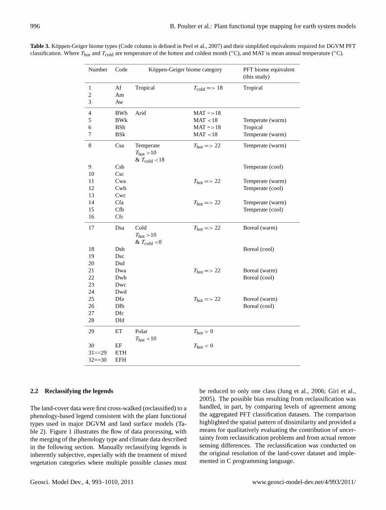
The Koppen-Geiger dataset was created by Peel etal. (2007) from over 4000 metrological stations contained inthe Global Historical Climatological Network v2.0 database.The authors calculated climate indices (i.e., seasonal means,minimums, and maximums) for the stations from precipita-tion and temperature for their entire time series (mostly, the20th century) and then interpolated to a 0.1◦ resolution grid(not accounting for elevation). These indices were classifiedinto one of 32 possible climate zones (Table 3) according tothe original Koppen-Geiger classification system (Koppen,1936).

The GLC2000 land-cover data were generated fromSPOT-VEGETATION (SPOT 4) and ATSR-2/DMSP sensorsand are available for most of the vegetated surface of theglobe (75◦ N to 56◦ S, excluding Antarctica) at 1 km resolu-

tion (Bartholome and Belward, 2005; Hugh et al., 2004). Thedata were collected between November 1999 and December2000. The GLC2000 classification (Table 4) was conductedby regional expert groups following an unsupervised clas-sification of 19 similar geographic regions using the LCCSnomenclature (22 categories for global purposes).

The GlobCover data became available in 2008 (Arino etal., 2008) and represent the highest-spatial resolution dataavailable for global extent at this time (0.3 km resolution).The classification system also follows the LCCS system(22 categories, Table 5) and the spectral data were acquiredfrom the MERIS sensor on-board the ENVISAT satellite be-tween June 2004 and December 2006. Individual pixels areclassified using unsupervised and supervised approaches onsub-global regional clusters.

Two versions of the EOS-MODIS land cover data(MOD12Q1), V004 and V005, were used in the analysis.These differ in several aspects, including temporal coverage,spatial resolution, and classification methodology, but bothuse the same 17 IGBP categories (Table 6) (Friedl et al.,2010). These land-cover classes were categorized using aglobally consistent supervised classification approach. V004is available globally at 1 km resolution from data acquired in2001 while V005 is available at 0.5 km resolution at annualresolution (starting in 2001). Both products have multiplelegends available, and here we worked with the IGBP leg-end (Table 6), the primary MODIS legend from which theother legends are derived and most relevant for reclassifyingto phenology categories (next section).

www.geosci-model-dev.net/4/993/2011/ Geosci. Model Dev., 4, 993–1010, 2011


Table 3. Koppen-Geiger biome types (Code column is defined in Peel et al., 2007) and their simplified equivalents required for DGVM PFTclassification. WhereThot andTcold are temperature of the hottest and coldest month (◦C), and MAT is mean annual temperature (◦C).

Number Code Koppen-Geiger biome category PFT biome equivalent(this study)

1 Af Tropical Tcold=> 18 Tropical2 Am3 Aw

4 BWh Arid MAT =>185 BWk MAT <18 Temperate (warm)6 BSh MAT =>18 Tropical7 BSk MAT <18 Temperate (warm)

8 Csa TemperateThot>10& Tcold<18

Thot=> 22 Temperate (warm)

9 Csb Temperate (cool)10 Csc11 Cwa Thot=> 22 Temperate (warm)12 Cwb Temperate (cool)13 Cwc14 Cfa Thot=> 22 Temperate (warm)15 Cfb Temperate (cool)16 Cfc

17 Dsa ColdThot>10& Tcold<0

Thot=> 22 Boreal (warm)

18 Dsb Boreal (cool)19 Dsc20 Dsd21 Dwa Thot=> 22 Boreal (warm)22 Dwb Boreal (cool)23 Dwc24 Dwd25 Dfa Thot=> 22 Boreal (warm)26 Dfb Boreal (cool)27 Dfc28 Dfd

29 ET PolarThot<10

Thot> 0

30 EF Thot< 031==29 ETH32==30 EFH

2.2 Reclassifying the legends

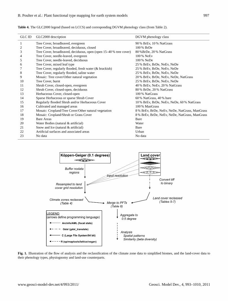
The land-cover data were first cross-walked (reclassified) to aphenology-based legend consistent with the plant functionaltypes used in major DGVM and land surface models (Ta-ble 2). Figure 1 illustrates the flow of data processing, withthe merging of the phenology type and climate data describedin the following section. Manually reclassifying legends isinherently subjective, especially with the treatment of mixedvegetation categories where multiple possible classes must

be reduced to only one class (Jung et al., 2006; Giri et al.,2005). The possible bias resulting from reclassification washandled, in part, by comparing levels of agreement amongthe aggregated PFT classification datasets. The comparisonhighlighted the spatial pattern of dissimilarity and provided ameans for qualitatively evaluating the contribution of uncer-tainty from reclassification problems and from actual remotesensing differences. The reclassification was conducted onthe original resolution of the land-cover dataset and imple-mented in C programming language.



Table 4. The GLC2000 legend (based on LCCS) and corresponding DGVM phenology class (from Table 2).

GLC ID GLC2000 description DGVM phenology class

1 Tree Cover, broadleaved, evergreen 90 % BrEv, 10 % NatGrass2 Tree Cover, broadleaved, deciduous, closed 100 % BrDe3 Tree Cover, broadleaved, deciduous, open (open 15–40 % tree cover) 80 %BrDe, 20 % NatGrass4 Tree Cover, needle-leaved, evergreen 100 % NeEv5 Tree Cover, needle-leaved, deciduous 100 % NeDe6 Tree Cover, mixed leaf type 25 % BrEv, BrDe, NeEv, NeDe7 Tree Cover, regularly flooded, fresh water (& brackish) 25 % BrEv, BrDe, NeEv, NeDe8 Tree Cover, regularly flooded, saline water 25 % BrEv, BrDe, NeEv, NeDe9 Mosaic: Tree cover/Other natural vegetation 20 % BrEv, BrDe, NeEv, NeDe, NatGrass10 Tree Cover, burnt 25 % BrEv, BrDe, NeEv, NeDe11 Shrub Cover, closed-open, evergreen 40 % BrEv, NeEv, 20 % NatGrass12 Shrub Cover, closed-open, deciduous 80 % BrDe, 20 % NatGrass13 Herbaceous Cover, closed-open 100 % NatGrass14 Sparse Herbaceous or sparse Shrub Cover 60 % NatGrass, 40 % bare15 Regularly flooded Shrub and/or Herbaceous Cover 10 % BrEv, BrDe, NeEv, NeDe, 60 % NatGrass16 Cultivated and managed areas 100 % ManGrass17 Mosaic: Cropland/Tree Cover/Other natural vegetation 8 % BrEv, BrDe, NeEv, NeDe, NatGrass, ManGrass18 Mosaic: Cropland/Shrub or Grass Cover 8 % BrEv, BrDe, NeEv, NeDe, NatGrass, ManGrass19 Bare Areas Bare20 Water Bodies (natural & artificial) Water21 Snow and Ice (natural & artificial) Bare22 Artificial surfaces and associated areas Urban23 No data No data

Fig. 1. Illustration of the flow of analysis and the reclassification of the climate zone data to simplified biomes, and the land-cover data totheir phenology types, physiognomy and land-use counterparts.



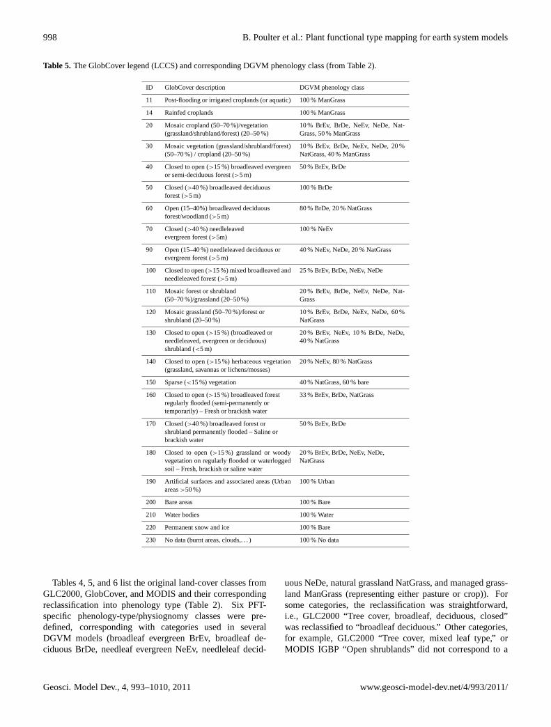
Table 5. The GlobCover legend (LCCS) and corresponding DGVM phenology class (from Table 2).

ID GlobCover description DGVM phenology class

11 Post-flooding or irrigated croplands (or aquatic) 100 % ManGrass

14 Rainfed croplands 100 % ManGrass

20 Mosaic cropland (50–70 %)/vegetation(grassland/shrubland/forest) (20–50 %)

10 % BrEv, BrDe, NeEv, NeDe, Nat-Grass, 50 % ManGrass

30 Mosaic vegetation (grassland/shrubland/forest)(50–70 %) / cropland (20–50 %)

10 % BrEv, BrDe, NeEv, NeDe, 20 %NatGrass, 40 % ManGrass

40 Closed to open (>15 %) broadleaved evergreenor semi-deciduous forest (>5 m)

50 % BrEv, BrDe

50 Closed (>40 %) broadleaved deciduousforest (>5 m)

100 % BrDe

60 Open (15–40%) broadleaved deciduousforest/woodland (>5 m)

80 % BrDe, 20 % NatGrass

70 Closed (>40 %) needleleavedevergreen forest (>5m)

100 % NeEv

90 Open (15–40 %) needleleaved deciduous orevergreen forest (>5 m)

40 % NeEv, NeDe, 20 % NatGrass

100 Closed to open (>15 %) mixed broadleaved andneedleleaved forest (>5 m)

25 % BrEv, BrDe, NeEv, NeDe

110 Mosaic forest or shrubland(50–70 %)/grassland (20–50 %)

20 % BrEv, BrDe, NeEv, NeDe, Nat-Grass

120 Mosaic grassland (50–70 %)/forest orshrubland (20–50 %)

10 % BrEv, BrDe, NeEv, NeDe, 60 %NatGrass

130 Closed to open (>15 %) (broadleaved orneedleleaved, evergreen or deciduous)shrubland (<5 m)

20 % BrEv, NeEv, 10 % BrDe, NeDe,40 % NatGrass

140 Closed to open (>15 %) herbaceous vegetation(grassland, savannas or lichens/mosses)

20 % NeEv, 80 % NatGrass

150 Sparse (<15 %) vegetation 40 % NatGrass, 60 % bare

160 Closed to open (>15 %) broadleaved forestregularly flooded (semi-permanently ortemporarily) – Fresh or brackish water

33 % BrEv, BrDe, NatGrass

170 Closed (>40 %) broadleaved forest orshrubland permanently flooded – Saline orbrackish water

50 % BrEv, BrDe

180 Closed to open (>15 %) grassland or woodyvegetation on regularly flooded or waterloggedsoil – Fresh, brackish or saline water

20 % BrEv, BrDe, NeEv, NeDe,NatGrass

190 Artificial surfaces and associated areas (Urbanareas>50 %)

100 % Urban

200 Bare areas 100 % Bare

210 Water bodies 100 % Water

220 Permanent snow and ice 100 % Bare

230 No data (burnt areas, clouds,. . . ) 100 % No data

Tables 4, 5, and 6 list the original land-cover classes fromGLC2000, GlobCover, and MODIS and their correspondingreclassification into phenology type (Table 2). Six PFT-specific phenology-type/physiognomy classes were pre-defined, corresponding with categories used in severalDGVM models (broadleaf evergreen BrEv, broadleaf de-ciduous BrDe, needleaf evergreen NeEv, needleleaf decid-

uous NeDe, natural grassland NatGrass, and managed grass-land ManGrass (representing either pasture or crop)). Forsome categories, the reclassification was straightforward,i.e., GLC2000 “Tree cover, broadleaf, deciduous, closed”was reclassified to “broadleaf deciduous.” Other categories,for example, GLC2000 “Tree cover, mixed leaf type,” orMODIS IGBP “Open shrublands” did not correspond to a



single PFT phenology/physiognomy class. In these cases, theland cover class was reclassified to one of several possiblephenology-types and physiognomy classes whose probabil-ity was assigned by assessing the supplementary data regard-ing the legend definitions or examining the spatial patternof observed land cover classes, and based on expert opinionon how the class might be composed of various phenologytypes (similar to Wang et al., 2006). In these cases, for ex-ample, a “mixed tree cover” category would yield 25 % equalprobability (using a uniform distribution for all mixed landcover categories) with the grid cell being reclassified to ei-ther BrEv, BrDe, NeEv, or NeDe. This approach resulted ina single category cell, but when the cells were aggregated tocoarser resolution (described below), the relative PFT frac-tions more realistically represented the original mixed for-est classes (for example, aggregating from 1 km mixed forestcategory to 0.5 degree resolution results in 0.5 degree frac-tions equal to 0.25 for BrEv, BrDe, NeEv, and NeDe, sum-ming to 1.0 for an aggregated cell).

2.3 Merging and aggregating phenology andclimate zones

The Koppen-Geiger dataset was first adjusted to expand itscoastal grid cell definitions to neighboring ocean grid cellsto allow a complete overlay of land cover with climate zone.The buffered Koppen-Geiger data were then downscaled tothe spatial resolution of the corresponding land-cover datasetusing a nearest neighbor resampling algorithm. The resam-pled Koppen-Geiger data were reclassified into one of threemajor biome types (following the rules described in Table 3),namely: tropical, temperate and boreal. The temperate andthe boreal biome were further subdivided into either cool(<22◦C) or warm (=>22◦C) types to distinguish betweenC3 or C4 photosynthesis in the former, and temperate needle-leaf and broadleaf trees in the latter (based on their PFTtemperature establishment thresholds in Table 2). While C4grasses can establish at cooler temperatures (i.e., the LPJmodel uses a temperature of 15◦C, Table 2), this tempera-ture threshold (22◦C) has been shown in prior studies to bea critical “crossover” temperature for C3 and C4 adaptations(Collatz et al., 1998).

Each of the 4 reclassified phenology type datasets werethen merged with the climate zones to produce the final PFTclassification at the spatial resolution of the original landcover data following the assembly rules in Table 7. Someexceptions were made to account for the full combinationof phenology and climate zone possibilities. For example,because there are few to no deciduous needleleaf PFTs ob-served in tropical and temperate ecosystems, this phenologytype was treated as tropical broadleaf raingreen (deciduous)or temperate broadleaf summergreen PFT. Natural and man-aged grasslands were split into the C3 and C4 photosyntheticpathways according to temperature thresholds that definedtropical versus temperate, and cool versus warm temperate

biomes from the Koppen-Geiger data. This approach mayunderestimate C3/C4 grass mixtures or C4 summer crops(i.e., maize) that might be planted in cooler regions (Ra-mankutty and Foley, 1998).

The PFT classifications were aggregated to a spatial reso-lution of 0.5◦ by summing the area of each PFT class withinthe corresponding 0.5◦ cell (16 classes, Table 7) and divid-ing by the grid cell area. A spatial resolution of 0.5◦ waschosen for this study because most models in the ESM com-munity use climate and other ancillary driver (e.g., soil type)data at this resolution, or greater (Zobler, 1986;New et al.,2002). The aggregation of PFT fractions can also be carriedout at finer resolution, but at smaller window sizes the es-timates of fractional PFT coverage may become more sen-sitive to the selection of probability distribution. Each ofthe four PFT fractional abundance files were filtered witha global land/water mask, which was derived from a globalsoils database (Zobler, 1986). This ensured that the terrestrialsurface area and land/ocean boundaries were equal betweendatasets.

2.4 Measuring PFT agreement

We analyzed the agreement between PFT fractional abun-dance (and re-groupings of PFTs by various traits) with abeta (ß) diversity metric (mean Euclidean distance) calcu-lated for each grid cell. Euclidean distance is a measure ofdissimilarity between groups with multiple members (Leg-endre et al., 2005) and is commonly used to summarize land-scape species diversity from multiple sampling plots (Whit-taker, 1972). In our case, the “plots” were the grid cellswhich contained the fractional PFT abundances containedfrom the different classification datasets. This analysis hadtwo objectives; the first was to assess, geographically, whereregions of high uncertainty in PFT abundance may exist, thesecond was to help evaluate the methods for the reclassifi-cation of legends, especially for the mixed vegetation cate-gories.

The beta diversity metric was calculated for each grid cellfor each of the four datasets, for the standard PFT classifica-tion, and for three re-groupings based on PFT traits. Theseregroupings were 1. Phenology type (total evergreen ver-sus total deciduous fraction), 2. Physiognomy (total woodyversus total herbaceous fraction), and 3. Management status(natural grass versus managed grass). Equation (1) presentsthe variables used for calculating the Euclidean distance,the mean of which, we consider to represent beta diversity,ß. For every grid cellc, the Euclidean distance,D wascalculated between every combination of classifications,N

(1. . . 4) composed of 10 PFTs (I = 10) and their correspond-ing fractional abundanceAfor the different classifications (j

andk).

ßc=Dc=

N∑n=1

[I∑

i=1

(Ai,j,c−Ai,k,c

)2]0.5

N(1)



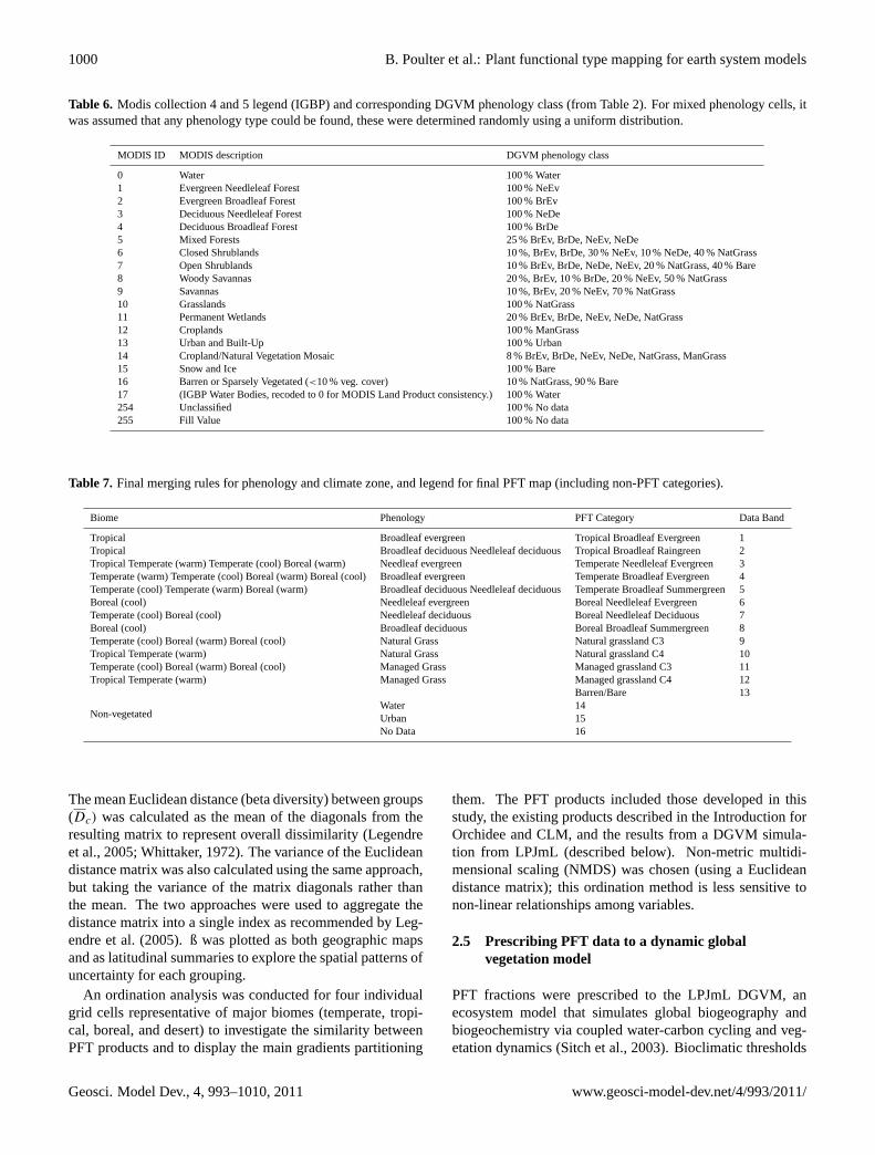
Table 6. Modis collection 4 and 5 legend (IGBP) and corresponding DGVM phenology class (from Table 2). For mixed phenology cells, itwas assumed that any phenology type could be found, these were determined randomly using a uniform distribution.

MODIS ID MODIS description DGVM phenology class

0 Water 100 % Water1 Evergreen Needleleaf Forest 100 % NeEv2 Evergreen Broadleaf Forest 100 % BrEv3 Deciduous Needleleaf Forest 100 % NeDe4 Deciduous Broadleaf Forest 100 % BrDe5 Mixed Forests 25 % BrEv, BrDe, NeEv, NeDe6 Closed Shrublands 10 %, BrEv, BrDe, 30 % NeEv, 10 % NeDe, 40 % NatGrass7 Open Shrublands 10 % BrEv, BrDe, NeDe, NeEv, 20 % NatGrass, 40 % Bare8 Woody Savannas 20 %, BrEv, 10 % BrDe, 20 % NeEv, 50 % NatGrass9 Savannas 10 %, BrEv, 20 % NeEv, 70 % NatGrass10 Grasslands 100 % NatGrass11 Permanent Wetlands 20 % BrEv, BrDe, NeEv, NeDe, NatGrass12 Croplands 100 % ManGrass13 Urban and Built-Up 100 % Urban14 Cropland/Natural Vegetation Mosaic 8 % BrEv, BrDe, NeEv, NeDe, NatGrass, ManGrass15 Snow and Ice 100 % Bare16 Barren or Sparsely Vegetated (<10 % veg. cover) 10 % NatGrass, 90 % Bare17 (IGBP Water Bodies, recoded to 0 for MODIS Land Product consistency.) 100 % Water254 Unclassified 100 % No data255 Fill Value 100 % No data

Table 7. Final merging rules for phenology and climate zone, and legend for final PFT map (including non-PFT categories).

Biome Phenology PFT Category Data Band

Tropical Broadleaf evergreen Tropical Broadleaf Evergreen 1Tropical Broadleaf deciduous Needleleaf deciduous Tropical Broadleaf Raingreen 2Tropical Temperate (warm) Temperate (cool) Boreal (warm) Needleaf evergreen Temperate Needleleaf Evergreen 3Temperate (warm) Temperate (cool) Boreal (warm) Boreal (cool) Broadleaf evergreen Temperate Broadleaf Evergreen 4Temperate (cool) Temperate (warm) Boreal (warm) Broadleaf deciduous Needleleaf deciduous Temperate Broadleaf Summergreen 5Boreal (cool) Needleleaf evergreen Boreal Needleleaf Evergreen 6Temperate (cool) Boreal (cool) Needleleaf deciduous Boreal Needleleaf Deciduous 7Boreal (cool) Broadleaf deciduous Boreal Broadleaf Summergreen 8Temperate (cool) Boreal (warm) Boreal (cool) Natural Grass Natural grassland C3 9Tropical Temperate (warm) Natural Grass Natural grassland C4 10Temperate (cool) Boreal (warm) Boreal (cool) Managed Grass Managed grassland C3 11Tropical Temperate (warm) Managed Grass Managed grassland C4 12

Non-vegetated

Barren/Bare 13Water 14Urban 15No Data 16

The mean Euclidean distance (beta diversity) between groups(Dc) was calculated as the mean of the diagonals from theresulting matrix to represent overall dissimilarity (Legendreet al., 2005; Whittaker, 1972). The variance of the Euclideandistance matrix was also calculated using the same approach,but taking the variance of the matrix diagonals rather thanthe mean. The two approaches were used to aggregate thedistance matrix into a single index as recommended by Leg-endre et al. (2005). ß was plotted as both geographic mapsand as latitudinal summaries to explore the spatial patterns ofuncertainty for each grouping.

An ordination analysis was conducted for four individualgrid cells representative of major biomes (temperate, tropi-cal, boreal, and desert) to investigate the similarity betweenPFT products and to display the main gradients partitioning

them. The PFT products included those developed in thisstudy, the existing products described in the Introduction forOrchidee and CLM, and the results from a DGVM simula-tion from LPJmL (described below). Non-metric multidi-mensional scaling (NMDS) was chosen (using a Euclideandistance matrix); this ordination method is less sensitive tonon-linear relationships among variables.

2.5 Prescribing PFT data to a dynamic globalvegetation model

PFT fractions were prescribed to the LPJmL DGVM, anecosystem model that simulates global biogeography andbiogeochemistry via coupled water-carbon cycling and veg-etation dynamics (Sitch et al., 2003). Bioclimatic thresholds



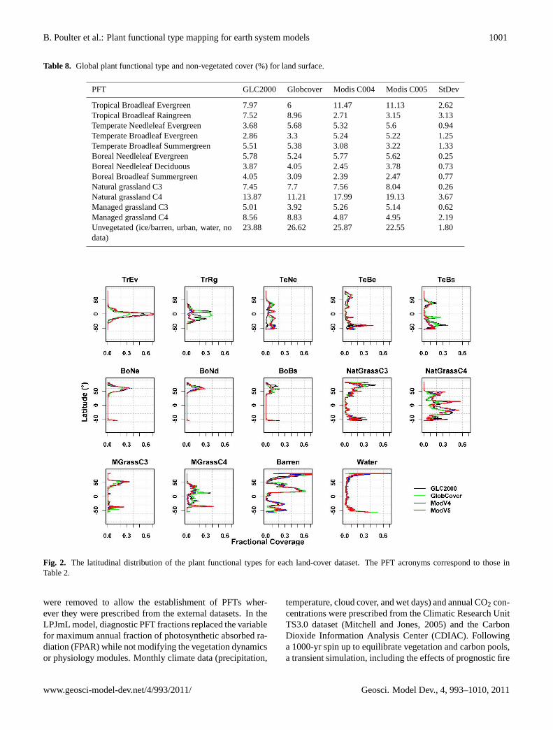
Table 8. Global plant functional type and non-vegetated cover (%) for land surface.

PFT GLC2000 Globcover Modis C004 Modis C005 StDev

Tropical Broadleaf Evergreen 7.97 6 11.47 11.13 2.62Tropical Broadleaf Raingreen 7.52 8.96 2.71 3.15 3.13Temperate Needleleaf Evergreen 3.68 5.68 5.32 5.6 0.94Temperate Broadleaf Evergreen 2.86 3.3 5.24 5.22 1.25Temperate Broadleaf Summergreen 5.51 5.38 3.08 3.22 1.33Boreal Needleleaf Evergreen 5.78 5.24 5.77 5.62 0.25Boreal Needleleaf Deciduous 3.87 4.05 2.45 3.78 0.73Boreal Broadleaf Summergreen 4.05 3.09 2.39 2.47 0.77Natural grassland C3 7.45 7.7 7.56 8.04 0.26Natural grassland C4 13.87 11.21 17.99 19.13 3.67Managed grassland C3 5.01 3.92 5.26 5.14 0.62Managed grassland C4 8.56 8.83 4.87 4.95 2.19Unvegetated (ice/barren, urban, water, nodata)

23.88 26.62 25.87 22.55 1.80

Fig. 2. The latitudinal distribution of the plant functional types for each land-cover dataset. The PFT acronyms correspond to those inTable 2.

were removed to allow the establishment of PFTs wher-ever they were prescribed from the external datasets. In theLPJmL model, diagnostic PFT fractions replaced the variablefor maximum annual fraction of photosynthetic absorbed ra-diation (FPAR) while not modifying the vegetation dynamicsor physiology modules. Monthly climate data (precipitation,

temperature, cloud cover, and wet days) and annual CO2 con-centrations were prescribed from the Climatic Research UnitTS3.0 dataset (Mitchell and Jones, 2005) and the CarbonDioxide Information Analysis Center (CDIAC). Followinga 1000-yr spin up to equilibrate vegetation and carbon pools,a transient simulation, including the effects of prognostic fire



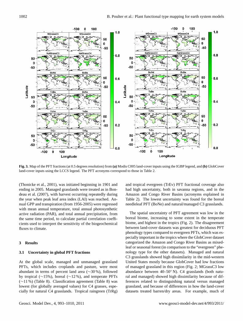
Fig. 3. Map of the PFT fractions (at 0.5 degrees resolution) from(a) Modis C005 land-cover inputs using the IGBP legend, and(b) GlobCoverland-cover inputs using the LCCS legend. The PFT acronyms correspond to those in Table 2.

(Thonicke et al., 2001), was initiated beginning in 1901 andending in 2005. Managed grasslands were treated as in Bon-deau et al. (2007), with harvest occurring repeatedly duringthe year when peak leaf area index (LAI) was reached. An-nual GPP and transpiration (from 1956-2005) were regressedwith mean annual temperature, total annual photosyntheticactive radiation (PAR), and total annual precipitation, fromthe same time period, to calculate partial correlation coeffi-cients used to interpret the sensitivity of the biogeochemicalfluxes to climate.

3 Results

3.1 Uncertainty in global PFT fractions

At the global scale, managed and unmanaged grasslandPFTs, which includes croplands and pasture, were mostabundant in terms of percent land area (∼30 %), followedby tropical (∼15%), boreal (∼12 %), and temperate PFTs(∼11 %) (Table 8). Classification agreement (Table 8) waslowest (for globally averaged values) for C4 grasses, espe-cially for natural C4 grasslands. Tropical raingreen (TrRg)

and tropical evergreen (TrEv) PFT fractional coverage alsohad high uncertainty, both in savanna regions, and in theAmazon and Congo River Basins (acronyms explained inTable 2). The lowest uncertainty was found for the borealneedleleaf PFT (BoNe) and natural/managed C3 grasslands.

The spatial uncertainty of PFT agreement was low in theboreal biome, increasing to some extent in the temperatebiome, and highest in the tropics (Fig. 2). The disagreementbetween land-cover datasets was greatest for deciduous PFTphenology types compared to evergreen PFTs, which was es-pecially important in the tropics where the GlobCover datasetcategorized the Amazon and Congo River Basins as mixed-leaf or seasonal forest (in comparison to the “evergreen” phe-nology type for the other datasets). Managed and naturalC3 grasslands showed high dissimilarity in the mid-westernUnited States mostly because GlobCover had low fractionsof managed grassland in this region (Fig. 2; MGrassC3 lowabundance between 40–50◦ N). C4 grasslands (both natu-ral and managed) showed high dissimilarity because of dif-ferences related to distinguishing natural versus managedgrassland, and because of differences in how the land-coverdatasets treated barren/dry areas. For example, much of



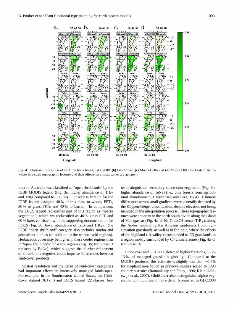
Fig. 4. Close-up illustration of PFT fractions for(a) GLC2000,(b) GlobCover,(c) Modis C004 and(d) Modis C005 for Eastern Africawhere fine-scale topographic features and their effects on climate zones are apparent.

interior Australia was classified as “open shrublands” by theIGBP MODIS legend (Fig. 3a; higher abundance of TrEvand TrRg compared to Fig. 3b). Our reclassification for theIGBP legend assigned 40 % of this class to woody PFTs,20 % to grass PFTs and 40 % to barren. In comparison,the LCCS legend reclassifies part of this region as “sparsevegetation”, which we reclassified as 40 % grass PFT and60 % bare, consistent with the supporting documentation forLCCS (Fig. 3b; lower abundance of TrEv and TrRg). TheIGBP “open shrubland” category also includes tundra andpermafrost biomes (in addition to the warmer arid regions).Herbaceous cover may be higher in these cooler regions thanin “open shrublands” of warm regions (Fig. 3b; NatGrassC3replaces by BoNe), which suggests that further refinementof shrubland categories could improve differences betweenland-cover products.

Spatial resolution and the detail of land-cover categorieshad important effects in intensively managed landscapes.For example, in the Southeastern United States, the Glob-Cover dataset (0.3 km) and LCCS legend (22 classes) bet-

ter distinguished secondary succession vegetation (Fig. 3b;higher abundance of TeNe) (i.e., pine forests from agricul-tural abandonment, Christensen and Peet, 1984). Climaticdifferences across small gradients were generally detected bythe Koppen-Geiger classification, despite elevation not beingincluded in the interpolation process. These topographic fea-tures were apparent in the north-south divide along the islandof Madagascar (Fig. 4a–d; NatGrassC4 versus TrRg), alongthe Andes, separating the Amazon rainforests from high-elevation grasslands, as well as in Ethiopia, where the effectsof the highland rift-valley corresponded to C3 grasslands ina region mostly surrounded by C4 climate zones (Fig. 4a–d;NatGrassC3).

GlobCover and GLC2000 detected higher fractions,∼12–13 %, of managed grasslands globally. Compared to theMODIS products, this estimate is slightly less than∼14 %for cropland area found in previous studies scaled to FAOcountry statistics (Ramankutty and Foley, 1998; Klein Gold-ewijk et al., 2007). GlobCover also distinguished alpine veg-etation communities in more detail (compared to GLC2000



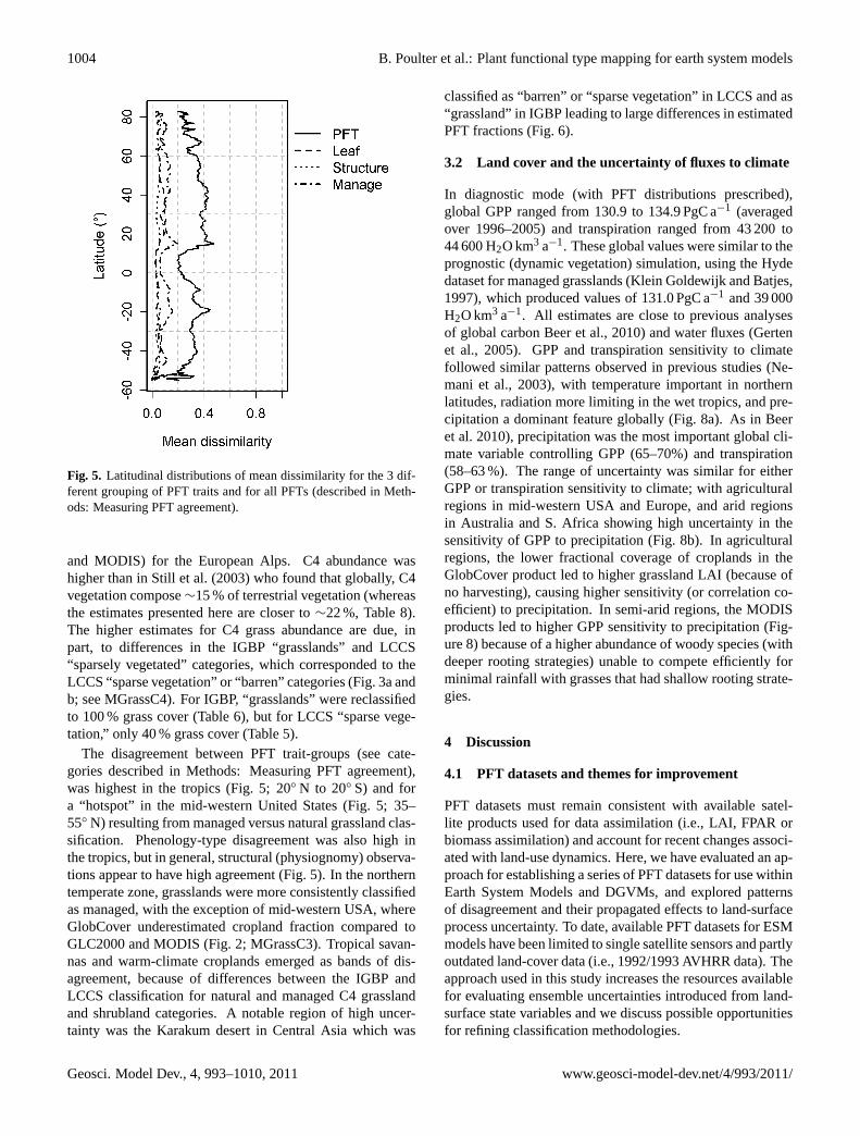
Fig. 5. Latitudinal distributions of mean dissimilarity for the 3 dif-ferent grouping of PFT traits and for all PFTs (described in Meth-ods: Measuring PFT agreement).

and MODIS) for the European Alps. C4 abundance washigher than in Still et al. (2003) who found that globally, C4vegetation compose∼15 % of terrestrial vegetation (whereasthe estimates presented here are closer to∼22 %, Table 8).The higher estimates for C4 grass abundance are due, inpart, to differences in the IGBP “grasslands” and LCCS“sparsely vegetated” categories, which corresponded to theLCCS “sparse vegetation” or “barren” categories (Fig. 3a andb; see MGrassC4). For IGBP, “grasslands” were reclassifiedto 100 % grass cover (Table 6), but for LCCS “sparse vege-tation,” only 40 % grass cover (Table 5).

The disagreement between PFT trait-groups (see cate-gories described in Methods: Measuring PFT agreement),was highest in the tropics (Fig. 5; 20◦ N to 20◦ S) and fora “hotspot” in the mid-western United States (Fig. 5; 35–55◦ N) resulting from managed versus natural grassland clas-sification. Phenology-type disagreement was also high inthe tropics, but in general, structural (physiognomy) observa-tions appear to have high agreement (Fig. 5). In the northerntemperate zone, grasslands were more consistently classifiedas managed, with the exception of mid-western USA, whereGlobCover underestimated cropland fraction compared toGLC2000 and MODIS (Fig. 2; MGrassC3). Tropical savan-nas and warm-climate croplands emerged as bands of dis-agreement, because of differences between the IGBP andLCCS classification for natural and managed C4 grasslandand shrubland categories. A notable region of high uncer-tainty was the Karakum desert in Central Asia which was

classified as “barren” or “sparse vegetation” in LCCS and as“grassland” in IGBP leading to large differences in estimatedPFT fractions (Fig. 6).

3.2 Land cover and the uncertainty of fluxes to climate

In diagnostic mode (with PFT distributions prescribed),global GPP ranged from 130.9 to 134.9 PgC a−1 (averagedover 1996–2005) and transpiration ranged from 43 200 to44 600 H2O km3 a−1. These global values were similar to theprognostic (dynamic vegetation) simulation, using the Hydedataset for managed grasslands (Klein Goldewijk and Batjes,1997), which produced values of 131.0 PgC a−1 and 39 000H2O km3 a−1. All estimates are close to previous analysesof global carbon Beer et al., 2010) and water fluxes (Gertenet al., 2005). GPP and transpiration sensitivity to climatefollowed similar patterns observed in previous studies (Ne-mani et al., 2003), with temperature important in northernlatitudes, radiation more limiting in the wet tropics, and pre-cipitation a dominant feature globally (Fig. 8a). As in Beeret al. 2010), precipitation was the most important global cli-mate variable controlling GPP (65–70%) and transpiration(58–63 %). The range of uncertainty was similar for eitherGPP or transpiration sensitivity to climate; with agriculturalregions in mid-western USA and Europe, and arid regionsin Australia and S. Africa showing high uncertainty in thesensitivity of GPP to precipitation (Fig. 8b). In agriculturalregions, the lower fractional coverage of croplands in theGlobCover product led to higher grassland LAI (because ofno harvesting), causing higher sensitivity (or correlation co-efficient) to precipitation. In semi-arid regions, the MODISproducts led to higher GPP sensitivity to precipitation (Fig-ure 8) because of a higher abundance of woody species (withdeeper rooting strategies) unable to compete efficiently forminimal rainfall with grasses that had shallow rooting strate-gies.

4 Discussion

4.1 PFT datasets and themes for improvement

PFT datasets must remain consistent with available satel-lite products used for data assimilation (i.e., LAI, FPAR orbiomass assimilation) and account for recent changes associ-ated with land-use dynamics. Here, we have evaluated an ap-proach for establishing a series of PFT datasets for use withinEarth System Models and DGVMs, and explored patternsof disagreement and their propagated effects to land-surfaceprocess uncertainty. To date, available PFT datasets for ESMmodels have been limited to single satellite sensors and partlyoutdated land-cover data (i.e., 1992/1993 AVHRR data). Theapproach used in this study increases the resources availablefor evaluating ensemble uncertainties introduced from land-surface state variables and we discuss possible opportunitiesfor refining classification methodologies.



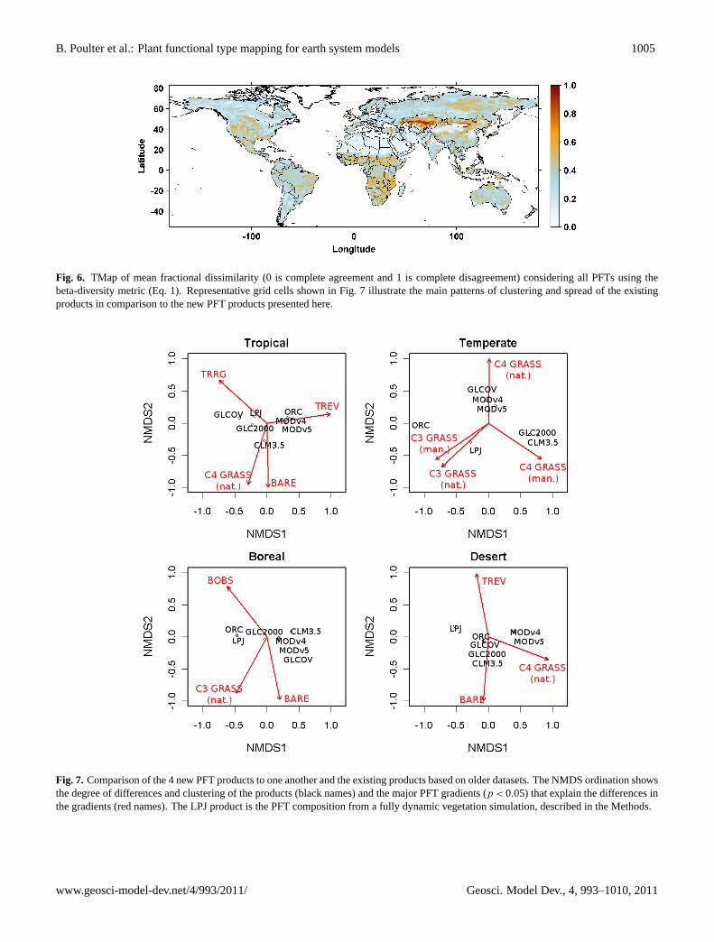
Fig. 6. TMap of mean fractional dissimilarity (0 is complete agreement and 1 is complete disagreement) considering all PFTs using thebeta-diversity metric (Eq. 1). Representative grid cells shown in Fig. 7 illustrate the main patterns of clustering and spread of the existingproducts in comparison to the new PFT products presented here.

Fig. 7. Comparison of the 4 new PFT products to one another and the existing products based on older datasets. The NMDS ordination showsthe degree of differences and clustering of the products (black names) and the major PFT gradients (p < 0.05) that explain the differences inthe gradients (red names). The LPJ product is the PFT composition from a fully dynamic vegetation simulation, described in the Methods.



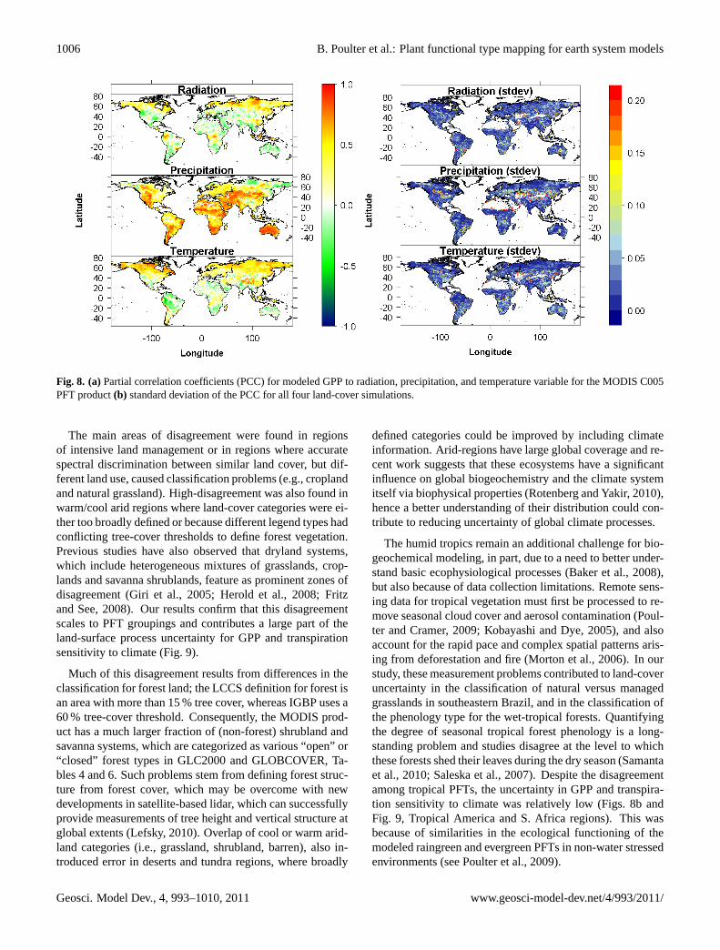
Fig. 8. (a)Partial correlation coefficients (PCC) for modeled GPP to radiation, precipitation, and temperature variable for the MODIS C005PFT product(b) standard deviation of the PCC for all four land-cover simulations.

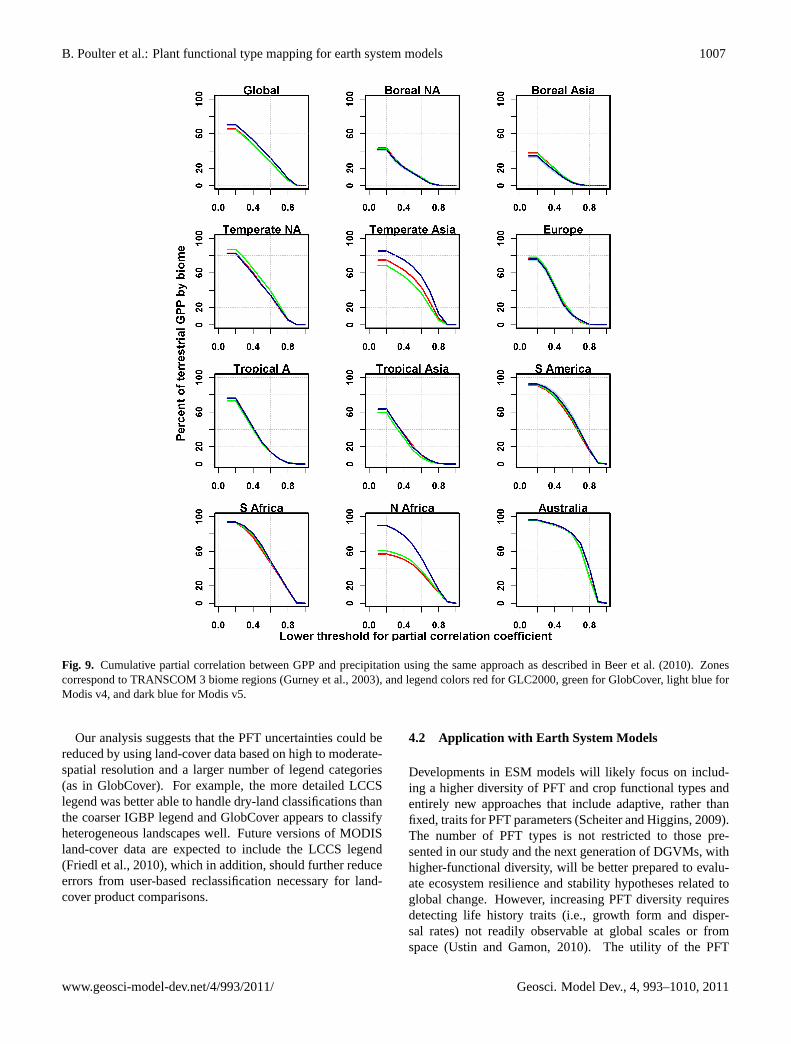
The main areas of disagreement were found in regionsof intensive land management or in regions where accuratespectral discrimination between similar land cover, but dif-ferent land use, caused classification problems (e.g., croplandand natural grassland). High-disagreement was also found inwarm/cool arid regions where land-cover categories were ei-ther too broadly defined or because different legend types hadconflicting tree-cover thresholds to define forest vegetation.Previous studies have also observed that dryland systems,which include heterogeneous mixtures of grasslands, crop-lands and savanna shrublands, feature as prominent zones ofdisagreement (Giri et al., 2005; Herold et al., 2008; Fritzand See, 2008). Our results confirm that this disagreementscales to PFT groupings and contributes a large part of theland-surface process uncertainty for GPP and transpirationsensitivity to climate (Fig. 9).

Much of this disagreement results from differences in theclassification for forest land; the LCCS definition for forest isan area with more than 15 % tree cover, whereas IGBP uses a60 % tree-cover threshold. Consequently, the MODIS prod-uct has a much larger fraction of (non-forest) shrubland andsavanna systems, which are categorized as various “open” or“closed” forest types in GLC2000 and GLOBCOVER, Ta-bles 4 and 6. Such problems stem from defining forest struc-ture from forest cover, which may be overcome with newdevelopments in satellite-based lidar, which can successfullyprovide measurements of tree height and vertical structure atglobal extents (Lefsky, 2010). Overlap of cool or warm arid-land categories (i.e., grassland, shrubland, barren), also in-troduced error in deserts and tundra regions, where broadly

defined categories could be improved by including climateinformation. Arid-regions have large global coverage and re-cent work suggests that these ecosystems have a significantinfluence on global biogeochemistry and the climate systemitself via biophysical properties (Rotenberg and Yakir, 2010),hence a better understanding of their distribution could con-tribute to reducing uncertainty of global climate processes.

The humid tropics remain an additional challenge for bio-geochemical modeling, in part, due to a need to better under-stand basic ecophysiological processes (Baker et al., 2008),but also because of data collection limitations. Remote sens-ing data for tropical vegetation must first be processed to re-move seasonal cloud cover and aerosol contamination (Poul-ter and Cramer, 2009; Kobayashi and Dye, 2005), and alsoaccount for the rapid pace and complex spatial patterns aris-ing from deforestation and fire (Morton et al., 2006). In ourstudy, these measurement problems contributed to land-coveruncertainty in the classification of natural versus managedgrasslands in southeastern Brazil, and in the classification ofthe phenology type for the wet-tropical forests. Quantifyingthe degree of seasonal tropical forest phenology is a long-standing problem and studies disagree at the level to whichthese forests shed their leaves during the dry season (Samantaet al., 2010; Saleska et al., 2007). Despite the disagreementamong tropical PFTs, the uncertainty in GPP and transpira-tion sensitivity to climate was relatively low (Figs. 8b andFig. 9, Tropical America and S. Africa regions). This wasbecause of similarities in the ecological functioning of themodeled raingreen and evergreen PFTs in non-water stressedenvironments (see Poulter et al., 2009).



Fig. 9. Cumulative partial correlation between GPP and precipitation using the same approach as described in Beer et al. (2010). Zonescorrespond to TRANSCOM 3 biome regions (Gurney et al., 2003), and legend colors red for GLC2000, green for GlobCover, light blue forModis v4, and dark blue for Modis v5.

Our analysis suggests that the PFT uncertainties could bereduced by using land-cover data based on high to moderate-spatial resolution and a larger number of legend categories(as in GlobCover). For example, the more detailed LCCSlegend was better able to handle dry-land classifications thanthe coarser IGBP legend and GlobCover appears to classifyheterogeneous landscapes well. Future versions of MODISland-cover data are expected to include the LCCS legend(Friedl et al., 2010), which in addition, should further reduceerrors from user-based reclassification necessary for land-cover product comparisons.

4.2 Application with Earth System Models

Developments in ESM models will likely focus on includ-ing a higher diversity of PFT and crop functional types andentirely new approaches that include adaptive, rather thanfixed, traits for PFT parameters (Scheiter and Higgins, 2009).The number of PFT types is not restricted to those pre-sented in our study and the next generation of DGVMs, withhigher-functional diversity, will be better prepared to evalu-ate ecosystem resilience and stability hypotheses related toglobal change. However, increasing PFT diversity requiresdetecting life history traits (i.e., growth form and disper-sal rates) not readily observable at global scales or fromspace (Ustin and Gamon, 2010). The utility of the PFT



approach for hypothesis testing and linkage to remote sens-ing will remain important. Finer resolution categories ofcrop types has been shown to be important for global bio-geochemical cycling (Bondeau et al., 2007) but crop typesor crop cover (or pasture) is not easily distinguished in theglobal land-cover datasets, highlighting the importance ofintegrated land-cover mapping approaches. Managed grass-land categories can be subdivided using regional statisticson crop use, similar to methods described by Ramankuttyet al. (1998), but many earth system models are at the earlystages of incorporating crop functional types.

By forcing LPJmL with diagnostic PFT fractions we wereable to illustrate the utility of ensembles of land-cover ap-proaches and the application of diagnostic datasets. Interest-ingly, global estimates of GPP and ET were similar, regard-less of land cover, confirming studies conducted at continen-tal scales (Jung et al., 2007). However, we show that thereare large regional differences, 20–30 %, in the sensitivity ofbiogeochemical fluxes to climate that are directly linked toland-cover uncertainty. High-PFT uncertainty did not alwayscorrespond to high biogeochemical cycling uncertainty (e.g.,wet tropics), illustrating that propagated errors may differfrom the initial condition agreement and that the choice ofevaluation metric is important. These PFT datasets have ap-plications beyond ESM modeling and can be integrated withbottom-up studies, include accounting methods for evaluat-ing carbon stocks (Kindermann et al., 2008), or as base-mapsthat can inform biodiversity-patterns related to biogeography(Loucks et al., 2008).

Acknowledgements.B. Poulter acknowledges funding from an FP7Marie Curie Incoming International Fellowship (Grant Number220546). NE Zimmermann and H Lischke acknowledge supportthrough the FP6 and FP7 projects ECOCHANGE (GOCE-CT-2007-036866) and MOTIVE (ENV-CT-2009-226544). E Hodsonacknowledges support from the MAIOLICA Project. The authorsare grateful for the development and distribution of the remotesensing datasets from European Commission’s Joint Research Cen-ter, Ispra, Italy, the European Space Agency, and Boston University.

Edited by: A. Stenke

The publication of this article is financed by CNRS-INSU.

References

Alton, P., Fisher, R. A., Los, S. O., and Williams, M.: Simulationsof global evapotranspiration using semiempirical and mechanis-tic schemes of plant hydrology, Global Biogeochem. Cy., 23,doi:10.1029/2009GB003540, 2009.

Arino, O., Bicheron, P., Achard, F., Latham, J., Witt, R., and Weber,J. L.: GLOBCOVER The most detailed portrait of Earth, ESABulletin-European Space Agency, 136, 24–31, 2008.

Baker, I. T., Prihodko, L., Denning, A. S., Goulden, M. L., Miller,S. D., and da Rocha, H. R.: Seasonal drought stress in the Ama-zon: Reconciling models and observations, J. Geophys. Res.,113,doi:10.1029/2007JG000644, 2008.

Bartholome, E. and Belward, A. S.: GLC2000: a new approach toglobal land cover mapping from Earth observation data, Int. J.Remote Sens., 26, 1959–1977, 2005.

Beer, C., Reichstein, M., Tomelleri, E., Ciais, P., Jung, M., Carval-hais, N., Rodenbeck, C., Arain, M. A., Baldocchi, D., Bonan,G., Bondeau, A., Cescatti, A., Lasslop, G., Lindroth, A., Lomas,M., Luyssaert, S., Margolis, H., Oleson, K. W., Roupsard, O.,Veenendaal, E., Viovy, N., Williams, C., Woodward, F. I., andPapale, D.: Terrestrial gross carbon dioxide uptake: Global dis-tribution and covariation with climate, Science, 329, 834–838,2010.

Bonan, G. B., Levis, S., Kergoat, L., and Oleson, K. W.: Land-scapes as patches of plant functional types: An integrating con-cept for climate and ecosystem models, Global Biogeochem. Cy.,16,doi:10.1029/2000GB001360, 2002.

Bondeau, A., Smith, P. C., Zaehle, S., Schaphoff, S., Lucht, W.,Cramer, W., Gerten, D., Lotze-Campen, H., Muller, C., Reich-stein, M., and Smith, B.: Modelling the role of agriculture forthe 20th century global carbon balance, Glob. Change Biol., 13,679–706, 2007.

Christensen, N. L. and Peet, R. K.: Convergence during secondaryforest succession, J. Ecol., 65, 25–36, 1984.

Collatz, G. J., Berry, J. A., and Clark, J. S.: Effects of climate andatmospheric CO2 partial pressure on the global distribution ofC4 grasses: Present, past, and future, Oecologia, 114, 441–454,1998.

DeFries, R., Hansen, M. C., Townshend, J. R. G., Janetos, A. C.,and Loveland, T. R.: A new global 1-km dataset of percentagetree cover derived from remote sensing, Glob. Change Biol., 6,247–254, 2000.

Dickinson, R. E., Oleson, K. W., Bonan, G. B., Hoffman, F., Thorn-ton, P. E., Vertenstein, M., Yang, Z. L., and Zeng, X.: The Com-munity Land Model and its climate statistics as a component ofthe Community Climate System Model, J. Climate, 19, 2302–2324, 2006.

Foley, J. A., Defries, R., Asner, G. P., Barford, C., Bonon, G., Car-penter, S. R., Chapin, F. S., Coe, M. T., Daily, G. C., Gibbs, H.K., Helkowski, J. H., Holloway, T., Howard, E. A., Kucharik, C.J., Monfreda, C., Patz, J. A., Prentice, I. C., Ramankutty, N., andSnyder, P. K.: Global consequences of land use, Science, 309,570–574, 2005.

Friedl, M. A., McIver, D. K., Hodges, J. C. F., Zhang, X. Y.,Muchoney, D., Strahler, A. H., Woodcock, C. E., Gopal, S.,Schneider, A., Cooper, A., Baccini, A., Gao, F., and Schaaf, C.B.: Global Land Cover Mapping from MODIS: Algorithms andEarly Results, Remote Sens. Environ., 83, 287–302, 2002.


http://dx.doi.org/10.1029/2009GB003540

http://dx.doi.org/10.1029/2007JG000644

http://dx.doi.org/10.1029/2000GB001360


Friedl, M. A., Sulla-Menashe, D., Tan, B., Schneider, A., Ra-mankutty, N., Sibley, A., and Huang, X.: MODIS Collection 5Global Land Cover: Algorithm refinements and characterizationof new datasets, Remote Sens. Environ., 114, 168–182, 2010.

Fritz, S. and See, L.: Identifying and quantifying uncertainty andspatial disagreement in the comparison of Global Land Coverfor different applications, Global Change Biol., 14, 1057–1075,2008.

Gerten, D., Hoff, H., Bondeau, A., Lucht, W., Smith, P., and Zaehle,S.: Contemporary “green” water flows: Simulations with a dy-namic global vegetation and water balance model, Phys. Chem.Earth, 30, 334–338, 2005.

Giri, C., Zhu, Z., and Reed, B.: A comparative analysis of theGlobal Land Cover 2000 and MODIS land cover data sets, Re-mote Sens. Environ., 94, 123–132, 2005.

Gurney, K. R., Law, R. M., Denning, A. S., Rayner, P., Baker, D.,Bousquet, P., Bruhwiler, L., Chen, Y. H., Ciais, P., Fan, S., Fung,I. Y., Gloor, M., Heimann, M., Higuchi, K., John, J., Kowal-czyk, E., Maki, T., Maksyutov, S., Peylin, P., Prather, M., Pak,B., Sarmiento, J., Taguchi, S., Takahashi, T., and Yuen, C. W.:TransCom 3 CO2 inversion intercomparison: 1. Annual meancontrol results and sensitivity to transport and prior flux informa-tion, Tellus, 55B, 555–579, 2003.

Haberl, H., Erb, K. H., Krausmann, F., Gaube, V., Bondeau, A.,Plutzar, C., Gingrich, S., Lucht, W., and Fischer-Kowalski, M.:Quantifying and mapping the human appropriation of net pri-mary production in earth’s terrestrial ecosystems, P. NationalAcademy of Science, 104, 12942–12947, 2007.

Herold, M., Mayaux, P., Woodcock, C. E., Baccini, A., and Schmul-lius, C.: Some challenges in global land cover mapping: An as-sessment of agreement and accuracy in existing 1 km datasets,Remote Sens. Environ., 112, 2538–2556, 2008.

Hugh, E. D., Belward, A., De Miranda, E. E., Di Bella, C. M.,Gond, V., Huber, O., Jones, S., Sgrenzaroli, M., and Fritz, S.:A land cover map of South America, Glob. Change Biol., 10,731–744, 2004.

Jung, M., Henkel, K., Herold, M., and Churkina, G.: Exploitingsynergies of global land cover products for carbon cycle model-ing, Remote Sens. Environ., 101, 534–553, 2006.

Jung, M., Vetter, M., Herold, M., Churkina, G., Reichstein, M., Za-ehle, S., Ciais, P., Viovy, N., Bondeau, A., Chen, Y., Trusilova,K., Feser, F., and Heimann, M.: Uncertainties of modeling grossprimary productivity over Europe: A systematic study on the ef-fects of using different drivers and terrestrial biosphere models,Glob. Biogeochem. Cy., 21,doi:10.1029/2006GB002915, 2007.

Kindermann, G., McCallum, I., Fritz, S., and Obersteiner, M.: AGlobal Forest Growing Stock, Biomass and Carbon Map Basedon FAO Statistics, Silva Fennica, 42, 387–396, 2008.

Kleidon, A., Adams, J., Pavlick, R., and Reu, B.: Simulated geo-graphic variations of plant species richness, evenness and abun-dance using climatic constraints on plant functional diversity, En-viron. Res. Lett., 4, 014007,doi:10.1088/1748-9326/4/1/014007,2009.

Klein Goldewijk, K. and Batjes, J. J.: A hundred year (1890–1990)database for integrated environmental assessments (HYDE, ver-sion 1.1), Bilthoven, the Netherlands, 1997.

Klein Goldewijk, K., van Drecht, G., and Bouwman, A. F.: Map-ping contemporary global cropland and grassland distributionson a 5 x 5 minute resolution, J. Land Use Sci., 2, 167–190, 2007.

Kobayashi, H. and Dye, D. G.: Atmospheric conditions for mon-itoring the long-term vegetation dynamics in the Amazon usingnormalized difference vegetation index, Remote Sens. Environ.,97, 519–525, 2005.

Koppen, W.: Das geographisca System der Klimate, in: Handbuchder Klimatologie, edited by: Koppen, W., and Geiger, G., 1. C.Gebr, Borntraeger, 1–44, 1936.

Krinner, G., Viovy, N., de Noblet-Ducoudre, N., Ogee, J., Polcher,J., Friedlingstein, P., Ciais, P., Sitch, S., and Prentice, I. C.:A dynamic global vegetation model for studies of the cou-pled atmosphere-biosphere system, Glob. Biogeochem. Cy., 19,GB1015, doi:1010.1029/2003GB002199, 2005.

Lapola, D. M., Oyama, M. D., Nobre, C. A., and Sampaio, G.:A new world natural vegetation map for global change studies,Annals of the Brazilian Academy of Science, 80, 397–408, 2008.

Lawrence, P. J. and Chase, T. N.: Representing a MODIS Consis-tent Land Surface in the Community Land Model (CLM 3.0):Part 1 Generating MODIS Consistent Land Surface Parameters,J. Geophys. Res., 112,doi:10.1029/2006JG000168, 2007.

Lefsky, M. A.: A global forest canopy height map from theModerate Resolution Imaging Spectroradiometer and the Geo-science Laser Altimeter System, Geophys. Res. Lett., 37,doi:10.1029/2010GL043622, 2010.

Legates, D. R. and Wilmott, C. J.: Mean seasonal and spatial vari-ability in global surface air temperature, Theor. Appl. Climatol.,41, 11–21, 1990.

Legendre, P., Borcard, D., and Peres-Neto, P. R.: Analyzing betadiversity: Partitioning the spatial variation of community com-position data, Ecol. Monogr., 75, 435–450, 2005.

Loucks, C. J., Ricketts, T. H., Naidoo, R., Lamoreux, J. F., andHoekstra, J. M.: Explaining the global pattern of protected areacoverage: relative importance of vertebrate biodiversity, humanactivities and agricultural suitability, J. Biogeogr., 35, 1337–1348, 2008.

Matthews, E.: Global vegetation and land use: New high-resolutiondata bases for climate studies, J. Clim. Appl. Meteorol., 22, 474–487, 1983.

Mitchell, C. D. and Jones, P.: An improved method of constructinga database of monthly climate observations and associated high-resolution grids, Int. J. Climatol., 25, 693–712, 2005.

Morton, D. C., DeFries, R. S., Shimabukuro, Y. E., Anderson, L. O.,Arai, E., del Bon Espirito-Santo, F., Freitas, R., and Morisette, J.T.: Cropland expansion changes deforestation dynamics in thesouthern Brazilian Amazon, P. National Academy of Science,103, 14637–14641 2006.

Nemani, R. R., Keeling, C. D., Hashimoto, H., Jolly, W. M., Piper,S. C., Tucker, C. J., Myneni, R. B., and Running, S.: Climate-Driven Increases in Global Terrestrial Net Primary Productionfrom 1982 to 1999, Science, 300, 1560–1563, 2003.

New, M., Lister, D., Hulme, M., and Makin, I.: A high-resolutiondata set of surface climate over global land areas, Clim. Res., 21,1-25, 2002.

Oki, T. and Kanae, S.: Global hydrological cycles and world waterresources, Science, 313, 1068–1072, 2006.

Olson, J., Watts, J. A., and Allison, L. J.: Carbon in Live Vegetationof Major World Ecosystems, ORNL-5862, Oak Ridge NationalLaboratory, Oak Ridge, Tennessee, 164 pp., 1983.

Peel, M. C., Finlayson, B. L., and McMahon, T. A.: Updatedworld map of the Kppen-Geiger climate classification, Hydrol.


http://dx.doi.org/10.1029/2006GB002915

http://dx.doi.org/10.1088/1748-9326/4/1/014007

http://dx.doi.org/10.1029/2006JG000168

http://dx.doi.org/10.1029/2010GL043622


Earth Syst. Sci., 11, 1633–1644,doi:10.5194/hess-11-1633-2007, 2007.

Plummer, S.: Perspectives on combining ecological process modelsand remotely sensed data, Ecol. Model., 129, 169–186, 2000.

Poulter, B. and Cramer, W.: Satellite remote sensing of tropicalforest canopies and their seasonal dynamics, Int. J. Remote Sens.,30, 6575–6590, 2009.

Poulter, B., Heyder, U., and Cramer, W.: Modelling the sensitivityof the seasonal cycle of GPP to dynamic LAI and soil depths intropical rainforests, Ecosystems, 12, 517–533, 2009.

Prentice, I. C., Cramer, W., Harrison, S. P., Leemans, R., Monserud,R. A., and Soloman, A. M.: A global biome model based onplant physiology and dominance, soil properties and climate, J.Biogeogr., 19, 117–134, 1992.

Quaife, T., Quegan, S., Disney, M., Lewis, P., Lomas, M. R., andWoodward, F. I.: Impact of land cover uncertainties on esti-mates of biospheric carbon fluxes, Glob. Biogeochem.l Cy., 22,doi:10.1029/2007GB003097, 2008.

Ramankutty, N. and Foley, J. A.: Characterizing patterns of globalland use: An analysis of global croplands data, Glob. Bio-geochem. Cy., 12, 667–685, 1998.

Rotenberg, E. and Yakir, D.: Contribution of semi-arid forests tothe climate system, Science, 327, 451–454, 2010.

Running, S., Loveland, T. R., Pierce, L. L., Nemani, R. R., andHunt, E. R.: A remote sensing based vegetation classificationlogic for global land cover analysis, Remote Sens. Environ., 51,39–48, 1995.

Saleska, S. R., Didan, K., Huete, A. R., and da Rocha, H. R.: Ama-zon forests green-up during 2005 drought, Science, 318, 612,2007.

Samanta, A., Ganguly, S., Hashimoto, H., Devadiga, S., Vermote, E.F., Knyazikhin, Y., Nemani, R. R., and Myneni, R. B.: Amazonforests did not green-up during the 2005 drought, Geophys. Res.Lett., 37, doi:10.1029/2009GL042154 2010.

Scheiter, S. and Higgins, S. I.: Impacts of climate change on thevegetation of Africa: an adaptive dynamic vegetation modellingapproach, Glob. Change Biol., 15, 2224–2246, 2009.

Schimel, D. S., House, J. I., Hibbard, K., Bousquet, P., Ciais, P.,Peylin, P., Braswell, B., Apps, M. J., Baker, D., Bondeau, A.,Canadell, J. G., Churkina, G., Cramer, W., Denning, A. S., Field,C. B., Friedlingstein, P., Goodale, C., Heimann, M., Houghton,R. A., Melillo, J. M., Moore III, B., Murdiyarso, D., Noble, I.P., S.W., Prentice, I. C., Raupach, M., Rayner, P., Scholes, R.J., Steffen, W., and Wirth, C.: Recent patterns and mechanismsof carbon exchange by terrestrial ecosystems, Nature, 414, 169–172, 2001.

Sitch, S., Smith, B., Prentice, I. C., Arneth, A., Bondeau, A.,Cramer, W., Kaplan, J. O., Levis, S., Lucht, W., Sykes, M. T.,Thonicke, K., and Venevsky, S.: Evaluation of ecosystem dy-namics, plant geography and terrestrial carbon cycling in the LPJdynamic global vegetation model, Glob. Change Biol., 9, 161–185, 2003.

Smith, T. M., Shugart, H. H., and Woodward, F. I.: Plant functionaltypes: their relevance to ecosystem properties and global change,Cambridge University Press, New York, 369 pp., 1997.

Sterling, S. and Ducharne, A.: Comprehensive data set of globalland cover change for land surface model applications, Glob.Biogeochem. Cy., 22,doi:10.1029/2007GB002959, 2008.

Still, C. J., Berry, J. A., Collatz, G. J., and DeFries, R.: Globaldistribution of C3 and C4 vegetation: Carbon cycle implications,Glob. Biogeochem. Cy., 17,doi:10.1029/2001GB001807, 2003.

Sun, W., Liang, S., Xu, G., Fang, H., and Dickinson, R. E.: Map-ping plant functional types from MODIS data using multisourceevidential reasoning, Remote Sens. Environ., 112, 1010–1024,2008.

Thonicke, K., Venevsky, S., Sitch, S., and Cramer, W.: The roleof fire disturbance for global vegetation dynamics: coupling fireinto a Dynamic Global Vegetation Model, Global Ecol. Bio-geogr., 10, 661–677, 2001.

Ustin, S. L. and Gamon, J. A.: Remote sensing of plant functionaltypes, New Phytologist, 186, 795–816, 2010.

Verant, S., Laval, K., Polcher, J., and De Castro, M.: Sensitivity ofthe continental hydrological cycle to the spatial resolution overthe Iberian Peninsula, J. Hydrometeorol., 5, 267–285, 2004.

Wang, A., Price, D. T., and Arora, V. K.: Estimating changes inglobal vegetation cover (1850-2100) for use in climate mod-els, Global Biogeochem. Cy., 20,doi:10.1029/2005GB002514,2006.

Whittaker, R. H.: Evolution and measurement of species diversity,Taxon, 21, 213–251, 1972.

Zobler, L.: A world soil file for global climate modeling, NASATechnical Memorandum, 32 pp., 1986.


http://dx.doi.org/10.5194/hess-11-1633-2007

http://dx.doi.org/10.5194/hess-11-1633-2007

http://dx.doi.org/10.1029/2007GB003097

http://dx.doi.org/10.1029/2007GB002959

http://dx.doi.org/10.1029/2001GB001807

http://dx.doi.org/10.1029/2005GB002514

Documents

Plant functional type mapping for earth system … · Plant functional type mapping for earth system models B. Poulter1,2, P. Ciais2, E. Hodson1, H. Lischke1, ... on the concept of