Playing Vivaldi in Hyperbolic Space

Cristian Lumezanu and Neil SpringUniversity of Maryland

{lume,nspring}@cs.umd.edu

Abstract

Internet coordinate systems have emerged as an efficient method to estimate the latencybetween pairs of nodes without any communication between them. They avoid the cost ofexplicit measurements by placing each node in a finite coordinate space and estimating thelatency between two nodes as the distance between their positions in the space. In this paper,we adapt the Vivaldi algorithm to use the Hyperbolic space for embedding. Researchers havefound promise in Hyperbolic space due to its mathematical elegance and its ability to modelthe structure of the Internet. We attempt to combine the elegance of the Hyperbolic space withthe practical, decentralized Vivaldi algorithm.

We evaluate both Euclidean and Hyperbolic Vivaldi on three sets of real-world latencies.Contrary to what we expected, we find that the performance of the two versions of Vivaldivaries with each data set. Furthermore, we show that the Hyperbolic coordinates have thetendency to underestimate large latencies (> 100 ms) but behave better when estimating shortdistances. Finally, we propose two distributed heuristics that help nodes decide whether tochoose Euclidean or Hyperbolic coordinates when estimating distances to their peers. Thisis the first comparison of Euclidean and Hyperbolic embeddings using the same distributedsolver and using a data set with more than 200 nodes.

1 IntroductionInternet coordinate systems estimate the latency between pairs of nodes without any communi-cation between them. They associate each node to a position in a finite coordinate space; thelatency between two nodes is then estimated as the distance between their positions in the space[10, 12, 20, 7, 9, 15, 2, 3]. Coordinate systems support wide-area applications and protocols thatallow the choice of communication peers based on the latency metric. For example, in the construc-tion of structured overlay networks [17, 14, 13], nodes usually select the closest peers to optimizequeries and responses. In file-sharing applications [5] or content distribution networks [4], it ismore efficient to download the required content from the server with the lowest latency [?].

Existing coordinate systems have three important components to their designs: space selec-tion, probing, and positioning. Space selection involves how to calculate the distances betweenpoints, whether the space is Euclidean, how many dimensions it has, etc. Probing is the process of

1

measuring latency to a few peers, or chosen landmarks. Positioning is the optimization process ofusing probe results to assign a location to every node in the space. These components determinewhether the system is accurate, scalable, and adaptive.

We separate these components so that we can reassemble a system that uses Hyperbolic spaceand the Vivaldi algorithm for probing and positioning. Vivaldi is distributed and adaptive, runningwithout global state and accommodating the dynamics of the network. Our choice for embeddingspace is based on the works of Shavitt and Tankel [16], Lua et al. [8], Subramanian et al. [19],and Tauro et al. [21]. Shavitt and Tankel use a centralized simulation-based algorithm to embednodes into a Hyperbolic space. They present good accuracy results later confirmed by the studyperformed by Lua et al.[8]. The Hyperbolic space, in which the distance between two nodes iscomputed along a curved line bent towards the origin, seems better fit for the jellyfish structure ofthe Internet (a core in the middle with many tendrils) [21].

We evaluate both Euclidean and Hyperbolic Vivaldi on three sets of latency measurements,two from King [6] between DNS servers and the third between PlanetLab nodes. Contrary towhat we expected, we find that the performance of the two versions of Vivaldi varies with eachdata set. We show that the PlanetLab data set behaves much worse in Hyperbolic space than inEuclidean space, while for one of the King data sets the Hyperbolic embedding is more accurate.Furthermore, our results show that Hyperbolic coordinates underestimate large latencies (> 100ms) but are more accurate in estimating distances between closer nodes. This is the first comparisonbetween Euclidean and Hyperbolic embeddings in a distributed setting and using a data set withmore than 200 nodes.

The rest of the paper is organized as follows. Section 2 gives a short overview on Hyper-bolic spaces and describes the changes we made to the Vivaldi algorithm. Section 3 presents theexperimental results. We conclude in Section 4.

2 Approach

2.1 Vivaldi algorithmWe use the same positioning algorithm as Dabek et al. [3]. We briefly and informally describe thealgorithm in this subsection.

Vivaldi simulates a physical system of springs where each spring corresponds to a pair ofnodes. The rest length of a spring emulates the real distance between two nodes while the actuallength is the distance computed by the embedding. The energy of each spring is proportional to itsdisplacement (the difference between the rest length and the current length). The algorithm runsiteratively at each node and simulates the progress of the springs toward a state with minimumenergy. At every step, each node will be pushed to a new position that minimizes the displacementof the springs it is connected to. Two factors affect the position of a node after each step ofthe algorithm: the magnitude (M ) and the direction (D) of the movement. The magnitude ofthe movement is proportional to the displacement of the associated springs and the direction ofmovement is given by the opposite of the gradient of the energy function with respect to the positionof the node. After computing the magnitude and the direction of movement the following rule

2

updates the coordinates of a node:x = x + δ ×M ×D

where δ is the timestep between two consecutive updates.We consider an n-dimensional coordinate space. The energy of a spring between nodes x =

(x1, x2, . . . , xn) and y = (y1, y2, . . . , yn) is:

Exy =1

2k(rttxy − d(x, y))2

where rttxy − d(x, y) is the displacement of the spring1 and k is the elasticity constant.

2.2 Euclidean VivaldiDabek et al. [3] use Euclidean distance:

d(x, y) =

√n∑

i=1

(xi − yi)2

After computing the gradient of the energy function, they obtain the following expressions for themagnitude and direction of movement:

D = u(x− y)

M =rttxy − d(x, y)√

n∑i=1

(xi − yi)2

where u is a unit vector.

2.3 Hyperbolic VivaldiWe now consider that the nodes and the conceptual springs lie instead in a Hyperbolic space.

It is hard for an observer in the three-dimensional Euclidean world to visualize and imagine theHyperbolic world [1]. To better analyze and understand it, different Euclidean models or maps ofthe Hyperbolic space have been constructed. As an analogy, people create maps that project pointsfrom the Earth sphere to a plane, which yields the familiar Mercator projection among others.Unfortunately, each model of the Hyperbolic geometry depicts a warped version of the Hyperbolicspace, just as a two-dimensional map represents the Earth in a distorted way.

To describe the Hyperbolic space, all we need to know is the amount of distortion introducedby the model used to embed the space. The distortion is determined by two parameters: curvatureand metric. Curvature is a characteristic of the space and represents the amount by which an objectin the space deviates from being flat. Euclidean spaces have curvature 0 because all lines areflat and Hyperbolic spaces have negative curvature. The metric is a characteristic of the modelused to embed the space and represents the distance function between two points in the model.

1We use subscripts to differentiate between a measured value (rttxy) and a computed value (d(x, y))

3

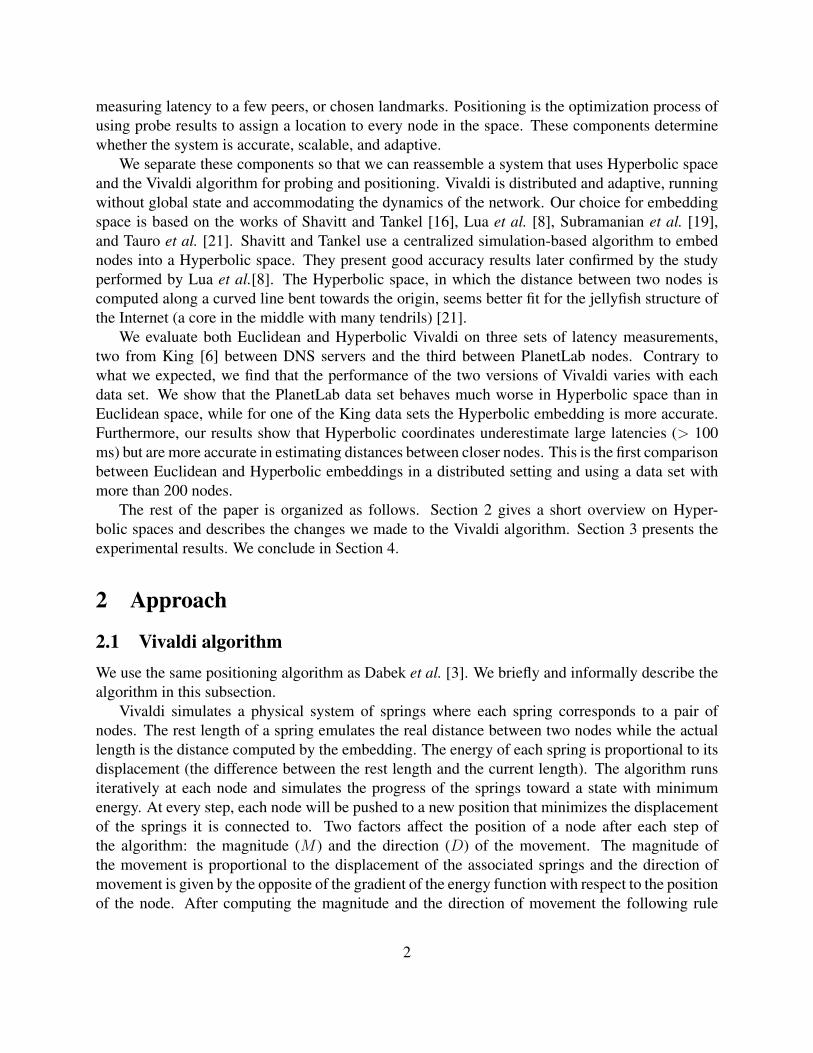
Figure 1: Hyperboloid with two sheets; the points in the Hyperbolic space are represented usingonly the upper sheet.

Knowing the curvature of a Hyperbolic space and the metric of its model we can determine thedistance between any two points in the space as well as the curved line along which the distance iscomputed.

The spring placed between the points will move along this curved line under a force propor-tional to the difference between the real distance and the Hyperbolic distance.

There are several equivalent models of the Hyperbolic world. We choose the hyperboloidmodel, in which all points lie on the upper sheet of a hyperboloid, due to the simplicity of itsmetric. Figure 1 presents a hyperboloid with two sheets. Although the model stretches to infinity,it is cut for observation. The distance between two points on the hyperboloid is computed along aline formed by the intersection of the hyperboloid with the plane determined by the two points andthe origin of the space.

The distance between points x=(x1, x2, . . . , xn) and y = (y1, y2, . . . , yn) in a n-dimensionalHyperbolic space of curvature k is:

d(x, y)=arccosh

(√(1+

n∑i=1

x2i )(1 +

n∑i=1

y2i )−

n∑i=1

xiyi

)×k

This formula is derived from the distance between two points on the unit hyperboloid (the arccoshpart) multiplied by the curvature of the Hyperbolic space (k).

The magnitude and direction of movement in the new space are computed using the gradientof the energy function.

D = u

(√1 +

∑ni=1 yi√

1 +∑n

i=1 xi

x− y

)

M =rttxy − d(x, y)√cosh2 d(x, y)− 1

3 ResultsIn this section, we compare the performance of Vivaldi in Euclidean and Hyperbolic spaces usingthree sets of real-world latencies. First, we present the data sets and the setup of the experiments.

4

0

0.5

1

1.5

2

2.5

3

0 200 400 600 800 1000

perc

ent o

f tot

al n

umbe

r of p

airs

RTT (ms)

PlanetLab192 (avg RTT = 192ms)King1740 (avg RTT = 180ms)King2500 (avg RTT = 78ms)

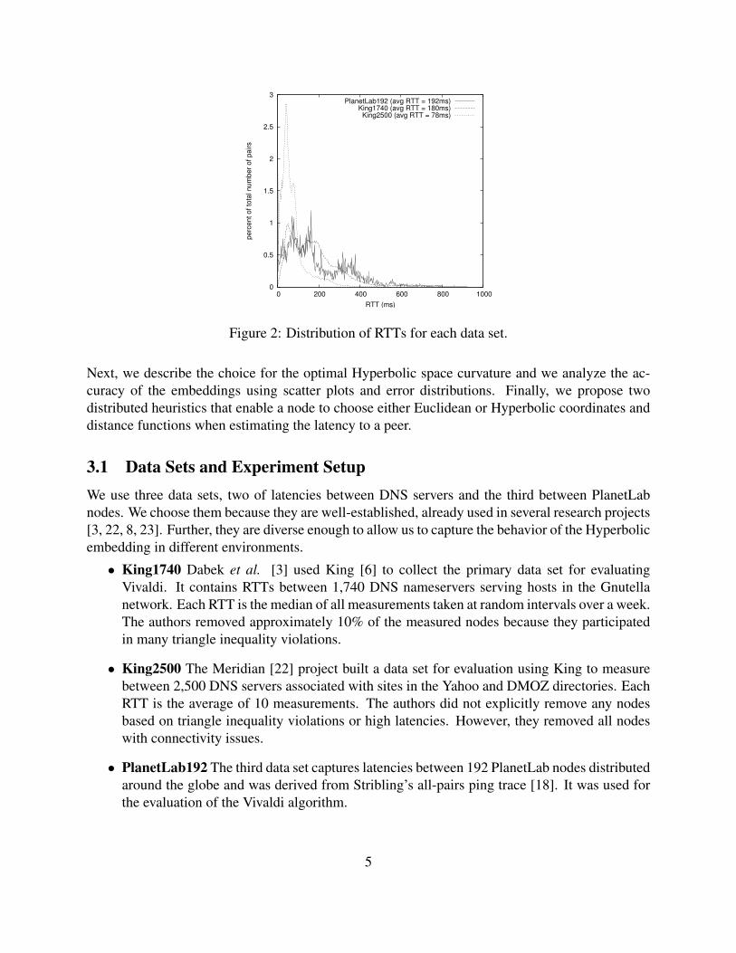
Figure 2: Distribution of RTTs for each data set.

Next, we describe the choice for the optimal Hyperbolic space curvature and we analyze the ac-curacy of the embeddings using scatter plots and error distributions. Finally, we propose twodistributed heuristics that enable a node to choose either Euclidean or Hyperbolic coordinates anddistance functions when estimating the latency to a peer.

3.1 Data Sets and Experiment SetupWe use three data sets, two of latencies between DNS servers and the third between PlanetLabnodes. We choose them because they are well-established, already used in several research projects[3, 22, 8, 23]. Further, they are diverse enough to allow us to capture the behavior of the Hyperbolicembedding in different environments.

• King1740 Dabek et al. [3] used King [6] to collect the primary data set for evaluatingVivaldi. It contains RTTs between 1,740 DNS nameservers serving hosts in the Gnutellanetwork. Each RTT is the median of all measurements taken at random intervals over a week.The authors removed approximately 10% of the measured nodes because they participatedin many triangle inequality violations.

• King2500 The Meridian [22] project built a data set for evaluation using King to measurebetween 2,500 DNS servers associated with sites in the Yahoo and DMOZ directories. EachRTT is the average of 10 measurements. The authors did not explicitly remove any nodesbased on triangle inequality violations or high latencies. However, they removed all nodeswith connectivity issues.

• PlanetLab192 The third data set captures latencies between 192 PlanetLab nodes distributedaround the globe and was derived from Stribling’s all-pairs ping trace [18]. It was used forthe evaluation of the Vivaldi algorithm.

5

We omit the details of the measurements that lead to the three data sets. The average round-triptimes are 180 ms, 74 ms and 190 ms, while the number of triples that violate the triangle inequalityamounts to 4%, 8%, and 5% of the triples in each data set. Figure 2 shows the distribution of RTTs;we plot the percentage of pairs for each round-trip time in the range from 1 to 1000 ms.

We use the MIT p2psim [11] packet-level network simulator. We modified the Vivaldi code toallow nodes to have two sets of coordinates: Euclidean and Hyperbolic. The Euclidean coordinatesare two-dimensional with a height vector, while the Hyperbolic coordinates have three dimensions.In this way, we ensure that a node has the same number of degrees of freedom in both spaces. Asthe algorithm runs, both coordinates are updated, allowing nodes to position themselves simul-taneously in Euclidean and Hyperbolic spaces. We fix the number of neighbors of each node to32: half are selected as the closest peers in network latency and the rest are selected at random.Similarly to the original Vivaldi algorithm, we use an adaptive timestep to help nodes find theirposition faster. We initialize both sets of coordinates for a node to the origin of the correspondingspace. We stop the algorithm after 10 seconds and collect the coordinates.

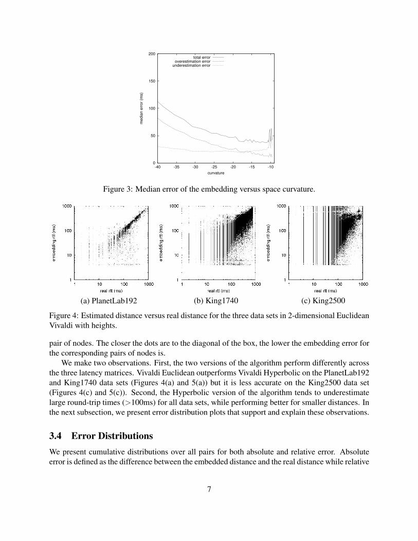
3.2 Curvature of the SpaceWe want to select the Hyperbolic space curvature that produces the lowest embedding error. Weshow how curvature affects the accuracy of the embedding of the PlanetLab192 data set in Figure 3.The horizontal axis represents the value of the curvature and the vertical axis is the median errorof the embedding. This is computed after the system has run for 10 seconds and represents theabsolute value of the difference between the embedding distance and the real distance. Longerruns than 10 seconds did not improve the median error significantly. Figure 3 indicates that thehigher the curvature of the embedding space, the lower the median error. To better analyze thisrelationship, we separate overestimation error from underestimation error. The overestimationerror is the median error of all the pairs for which the embedding distance is greater than thereal distance, while the underestimation error is the median error of the pairs whose real distanceis underestimated. The overestimation error decreases with the curvature of the space, while theunderestimation error is lowest around curvature -17 and grows gradually in both directions startingfrom this value. The plot also indicates that any curvature in the range -20 to -11 will produce alow embedding error. We choose the curvature for the embedding of the PlanetLab192 data setto be -14. Based on similar results, we set the curvatures for the King1740 and King2500 datasets to be -16 and -7. We believe that the King2500 requires a smaller absolute value for thecurvature because, on the average, it contains smaller latencies that need to be modeled. We usedifferent curvatures for the three data sets because we want to obtain the best possible Hyperbolicembeddings.

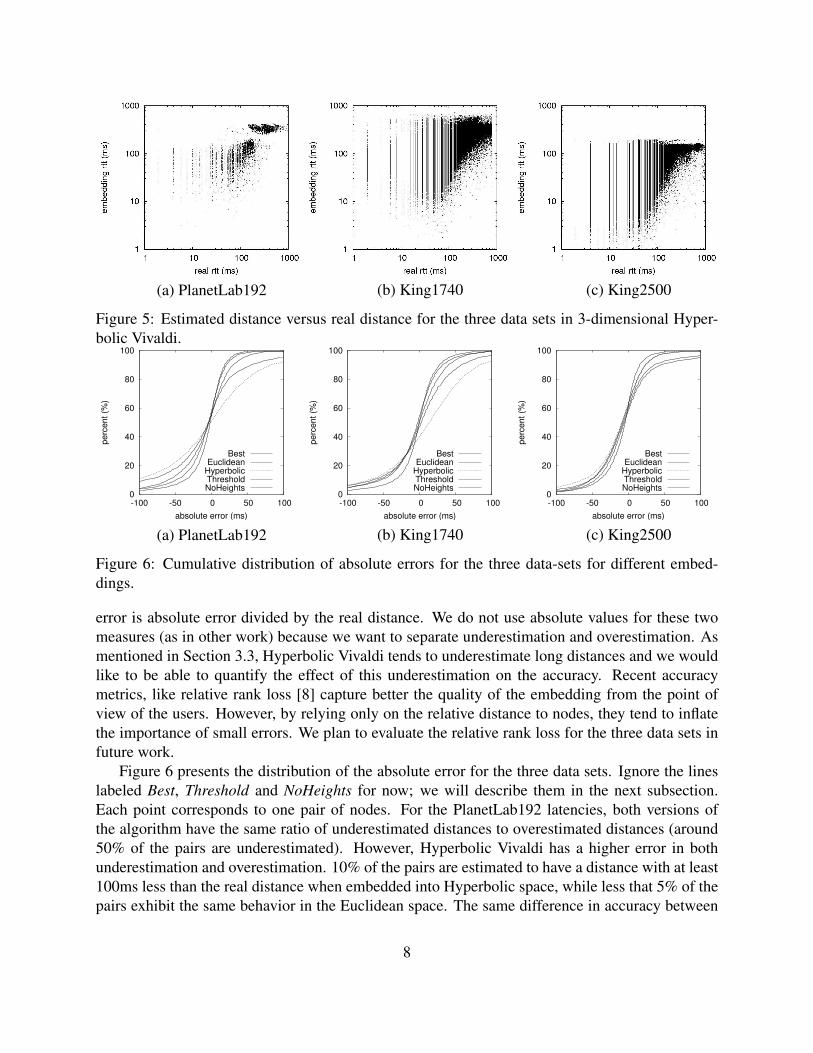
3.3 Latency estimationWe evaluate the accuracy of Vivaldi in Euclidean and Hyperbolic spaces by capturing the rela-tionship between the real and the estimated distances using scatter plots. Figures 4 and 5 presentscatter plots in which the horizontal axis is the measured round-trip time and the vertical axis cor-responds to the estimated distances. The axes have a logarithmic scale and each dot represents a

6

0

50

100

150

200

-40 -35 -30 -25 -20 -15 -10

med

ian

erro

r (m

s)

curvature

total erroroverestimation error

underestimation error

Figure 3: Median error of the embedding versus space curvature.

(a) PlanetLab192 (b) King1740 (c) King2500

Figure 4: Estimated distance versus real distance for the three data sets in 2-dimensional EuclideanVivaldi with heights.

pair of nodes. The closer the dots are to the diagonal of the box, the lower the embedding error forthe corresponding pairs of nodes is.

We make two observations. First, the two versions of the algorithm perform differently acrossthe three latency matrices. Vivaldi Euclidean outperforms Vivaldi Hyperbolic on the PlanetLab192and King1740 data sets (Figures 4(a) and 5(a)) but it is less accurate on the King2500 data set(Figures 4(c) and 5(c)). Second, the Hyperbolic version of the algorithm tends to underestimatelarge round-trip times (>100ms) for all data sets, while performing better for smaller distances. Inthe next subsection, we present error distribution plots that support and explain these observations.

3.4 Error DistributionsWe present cumulative distributions over all pairs for both absolute and relative error. Absoluteerror is defined as the difference between the embedded distance and the real distance while relative

7

(a) PlanetLab192 (b) King1740 (c) King2500

Figure 5: Estimated distance versus real distance for the three data sets in 3-dimensional Hyper-bolic Vivaldi.

0

20

40

60

80

100

-100 -50 0 50 100

perc

ent (

%)

absolute error (ms)

BestEuclidean

HyperbolicThresholdNoHeights

0

20

40

60

80

100

-100 -50 0 50 100

perc

ent (

%)

absolute error (ms)

BestEuclidean

HyperbolicThresholdNoHeights

0

20

40

60

80

100

-100 -50 0 50 100

perc

ent (

%)

absolute error (ms)

BestEuclidean

HyperbolicThresholdNoHeights

(a) PlanetLab192 (b) King1740 (c) King2500

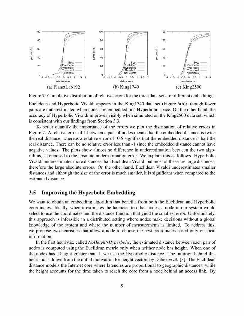
Figure 6: Cumulative distribution of absolute errors for the three data-sets for different embed-dings.

error is absolute error divided by the real distance. We do not use absolute values for these twomeasures (as in other work) because we want to separate underestimation and overestimation. Asmentioned in Section 3.3, Hyperbolic Vivaldi tends to underestimate long distances and we wouldlike to be able to quantify the effect of this underestimation on the accuracy. Recent accuracymetrics, like relative rank loss [8] capture better the quality of the embedding from the point ofview of the users. However, by relying only on the relative distance to nodes, they tend to inflatethe importance of small errors. We plan to evaluate the relative rank loss for the three data sets infuture work.

Figure 6 presents the distribution of the absolute error for the three data sets. Ignore the lineslabeled Best, Threshold and NoHeights for now; we will describe them in the next subsection.Each point corresponds to one pair of nodes. For the PlanetLab192 latencies, both versions ofthe algorithm have the same ratio of underestimated distances to overestimated distances (around50% of the pairs are underestimated). However, Hyperbolic Vivaldi has a higher error in bothunderestimation and overestimation. 10% of the pairs are estimated to have a distance with at least100ms less than the real distance when embedded into Hyperbolic space, while less that 5% of thepairs exhibit the same behavior in the Euclidean space. The same difference in accuracy between

8

0

20

40

60

80

100

-2 -1.5 -1 -0.5 0 0.5 1 1.5 2

perc

ent (

%)

relative error

BestEuclidean

HyperbolicThresholdNoHeights

0

20

40

60

80

100

-2 -1.5 -1 -0.5 0 0.5 1 1.5 2

perc

ent (

%)

relative error

BestEuclidean

HyperbolicThresholdNoHeights

0

20

40

60

80

100

-2 -1.5 -1 -0.5 0 0.5 1 1.5 2

perc

ent (

%)

relative error

BestEuclidean

HyperbolicThresholdNoHeights

(a) PlanetLab192 (b) King1740 (c) King2500

Figure 7: Cumulative distribution of relative errors for the three data-sets for different embeddings.

Euclidean and Hyperbolic Vivaldi appears in the King1740 data set (Figure 6(b)), though fewerpairs are underestimated when nodes are embedded in a Hyperbolic space. On the other hand, theaccuracy of Hyperbolic Vivaldi improves visibly when simulated on the King2500 data set, whichis consistent with our findings from Section 3.3.

To better quantify the importance of the errors we plot the distribution of relative errors inFigure 7. A relative error of 1 between a pair of nodes means that the embedded distance is twicethe real distance, whereas a relative error of -0.5 signifies that the embedded distance is half thereal distance. There can be no relative error less than -1 since the embedded distance cannot havenegative values. The plots show almost no difference in underestimation between the two algo-rithms, as opposed to the absolute underestimation error. We explain this as follows. HyperbolicVivaldi underestimates more distances than Euclidean Vivaldi but most of these are large distances,therefore the large absolute errors. On the other hand, Euclidean Vivaldi underestimates smallerdistances and although the size of the error is much smaller, it is significant when compared to theestimated distance.

3.5 Improving the Hyperbolic EmbeddingWe want to obtain an embedding algorithm that benefits from both the Euclidean and Hyperboliccoordinates. Ideally, when it estimates the latencies to other nodes, a node in our system wouldselect to use the coordinates and the distance function that yield the smallest error. Unfortunately,this approach is infeasible in a distributed setting where nodes make decisions without a globalknowledge of the system and where the number of measurements is limited. To address this,we propose two heuristics that allow a node to choose the best coordinates based only on localinformation.

In the first heuristic, called NoHeightsHyperbolic, the estimated distance between each pair ofnodes is computed using the Euclidean metric only when neither node has height. When one ofthe nodes has a height greater than 1, we use the Hyperbolic distance. The intuition behind thisheuristic is drawn from the initial motivation for height vectors by Dabek et al. [3]. The Euclideandistance models the Internet core where latencies are proportional to geographic distances, whilethe height accounts for the time taken to reach the core from a node behind an access link. By

9

using Hyperbolic distance estimation whenever a node has height, we offer an alternative to theVivaldi’s height model.

The second heuristic, ThresholdHyperbolic is partly based on the observations made in Sec-tion 3.3. Since Hyperbolic space seems to underestimate larger latencies, we choose Euclideandistance estimation for every pair whose Hyperbolic distance is computed to be more than a cer-tain threshold. In the experiments we used a threshold value of 100ms.

The absolute and relative error distributions of the embeddings using the two heuristics arelabeled NoHeights and Threshold in Figures 6 and 7. We denote by Best the embedding in which,for every pair, the distance with the smallest estimation error is chosen. The ThresholdHyperbolicembedding improves the accuracy of the pure Hyperbolic embedding and, as expected, eliminatesalmost completely the difference in underestimation when compared to the Euclidean embedding.It proves to be a more general alternative than Euclidean Vivaldi due to the good accuracy itachieves for all the data sets.

4 Conclusions and Future WorkWe have successfully adapted the Vivaldi algorithm so that nodes position themselves in a Hy-perbolic space. We compared the performance of Euclidean and Hyperbolic embeddings usingthree different data sets, two derived from the King measurement tool, the other composed oflatency measurements between PlanetLab nodes. Our results show the that accuracy of the twoversions of Vivaldi varies with each data set and that the Hyperbolic coordinates have the tendencyto underestimate large latencies. Based on these observations, we present a distributed heuris-tic, ThresholdHyperbolic, that uses both Euclidean and Hyperbolic coordinates and achieves goodaccuracy for all data sets.

In the future, we plan to extend our comparison to include the BBS Hyperbolic [16], a cen-tralized simulation-based network coordinate system that also uses Hyperbolic embedding. Inparticular, we are interested in evaluating how, if at all, the performance of the Hyperbolic em-bedding is influenced by a distributed deployment. We also intend to understand more completelythe behavior of Hyperbolic Vivaldi and of the two heuristics by evaluating their accuracy based onhow the embedding modifies the relative distance among nodes [8].

AcknowledgmentsWe thank Eng Keong Lua for our discussions and for his comments on an initial draft of this paper.

References[1] E. A. Abbott. Flatland: A Romance of Many Dimensions. publisher unknown, 1880.

[2] M. Costa, M. Castro, A. Rowstron, and P. Key. PIC: Practical Internet coordinates for distanceestimation. In ICDCS, 2004.

10

[3] F. Dabek, R. Cox, F. Kaashoek, and R. Morris. Vivaldi: a decentralized network coordinatesystem. In SIGCOMM, 2004.

[4] M. J. Freedman, E. Freudenthal, and D. Mazieres. Democratizing content publication withCoral. In NSDI, 2004.

[5] Gnutella. http://www.gnutella.com.

[6] K. Gummadi, S. Saroiu, and S. Gribble. King: Estimating latency between arbitrary Internetend hosts. In IMW, 2002.

[7] H. Lim, J. C. Hou, and C.-H. Choi. Constructing internet coordinate system based on delaymeasurement. In IMC, 2003.

[8] E. K. Lua, T. Griffin, M. Pias, H. Zheng, and J. Crowcroft. On the accuracy of the embeddingsfor Internet coordinate systems. In IMC, 2005.

[9] Y. Mao and L. K. Saul. Modeling distances in large-scale networks by matrix factorization.In IMC, 2004.

[10] T. S. E. Ng and H. Zhang. Predicting Internet network distance with coordinates-based ap-proaches. In INFOCOM, 2002.

[11] P2PSim. http://pdos.csail.mit.edu/p2psim.

[12] M. Pias, J. Crowcroft, S. Wilbur, T. Harris, and S. Bhatti. Lighthouses for scalable distributedlocation. In IPTPS, 2003.

[13] S. Ratnasamy, P. Francis, M. Handley, R. Karp, and S. Schenker. A scalable content-addressable network. In SIGCOMM, pages 161–172, 2001.

[14] A. Rowstron and P. Druschel. Pastry: Scalable, distributed object location and routing forlarge-scale peer-to-peer systems. In Proceedings of IFIP/ACM International Conference onDistributed Systems, 2001.

[15] Y. Shavitt and T. Tankel. Big-bang simulation for embedding network distances in euclideanspace. In INFOCOM, 2003.

[16] Y. Shavitt and T. Tankel. On the curvature of the Internet and its usage for overlay construc-tion and distance estimation. In INFOCOM, 2004.

[17] I. Stoica, R. Morris, D. Karger, M. F. Kaashoek, and H. Balakrishnan. Chord: A scalablepeer-to-peer lookup service for Internet applications. In SIGCOMM, 2001.

[18] J. Stribling. Planetlab all pairs ping. http://www.pdos.lcs.mit.edu/∼strib/pl app/.

[19] L. Subramanian, S. Agarwal, J. Rexford, and R. H. Katz. Characterizing the internet hierarchyfrom multiple vantage points. In Proceedings of INFOCOM, 2002.

11

[20] L. Tang and M. Crovella. Virtual landmarks for the internet. In IMC, 2003.

[21] S. Tauro, C. Palmer, G. Siganos, and M. Faloutsos. A simple conceptual model for the internettopology. In Global Internet, 2001.

[22] B. Wong, A. Slivkins, and E. G. Sirer. Meridian: A lightweight network location servicewithout virtual coordinates. In ACM SIGCOMM, 2005.

[23] R. Zhang, Y. C. Hu, Z. Lin, and S. Fahmy. A hierarchical approach to internet distanceprediction. In IEEE ICDCS, 2006.

12