Please turn off cell phones, pagers, etc.The lecture will begin shortly.

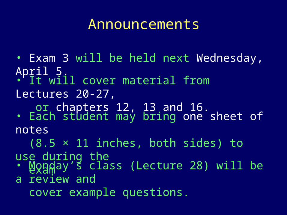
Announcements

• Exam 3 will be held next Wednesday, April 5.• It will cover material from Lectures 20-27, or chapters 12, 13 and 16.

• Monday’s class (Lecture 28) will be a review and cover example questions.

• Each student may bring one sheet of notes (8.5 × 11 inches, both sides) to use during the exam

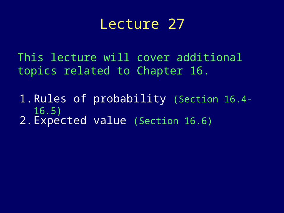
Lecture 27

This lecture will cover additional topics related to Chapter 16.

1. Rules of probability (Section 16.4-16.5)

2. Expected value (Section 16.6)

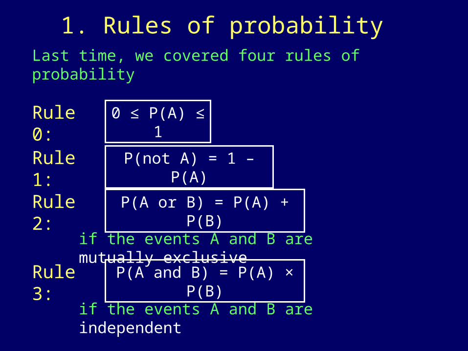
1. Rules of probabilityLast time, we covered four rules of probability

Rule 0: 0 ≤ P(A) ≤ 1

Rule 1: P(not A) = 1 – P(A)

Rule 2: P(A or B) = P(A) + P(B)

if the events A and B are mutually exclusive

Rule 3: P(A and B) = P(A) × P(B)

if the events A and B are independent

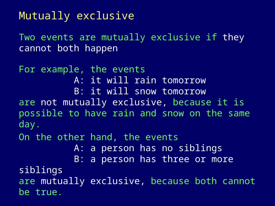
Mutually exclusive

Two events are mutually exclusive if they cannot both happen

For example, the eventsA: it will rain tomorrowB: it will snow tomorrow

are not mutually exclusive, because it is possible to have rain and snow on the same day.

On the other hand, the eventsA: a person has no siblingsB: a person has three or more siblings

are mutually exclusive, because both cannot be true.

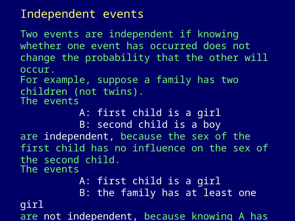
Independent events

Two events are independent if knowing whether one event has occurred does not change the probability that the other will occur.

The eventsA: first child is a girlB: second child is a boy

are independent, because the sex of the first child has no influence on the sex of the second child.

The eventsA: first child is a girlB: the family has at least one girl

are not independent, because knowing A has occurred increases the probability of B.

For example, suppose a family has two children (not twins).

Comments

• If two events are mutually exclusive, they cannot be independent.• If two events are independent, they cannot be mutually exclusive.

• Don’t fall prey to the gambler’s fallacy.

The gambler’s fallacy arises when a person erroneously believes that independent events influence each other.For example, the person may believe that he’s “due” to win the lottery soon, because he hasn’t won in a long time.

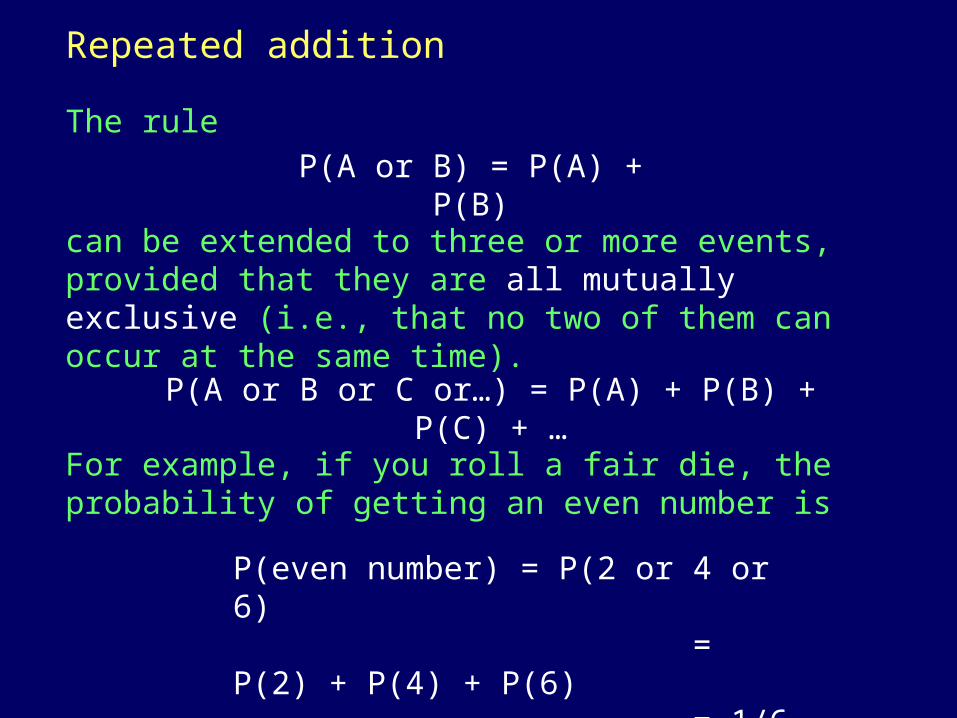
Repeated addition

The rule

can be extended to three or more events, provided that they are all mutually exclusive (i.e., that no two of them can occur at the same time).

P(A or B) = P(A) + P(B)

P(A or B or C or…) = P(A) + P(B) + P(C) + …

For example, if you roll a fair die, the probability of getting an even number is

P(even number) = P(2 or 4 or 6) = P(2) + P(4) + P(6) = 1/6 + 1/6 + 1/6 = 1/2

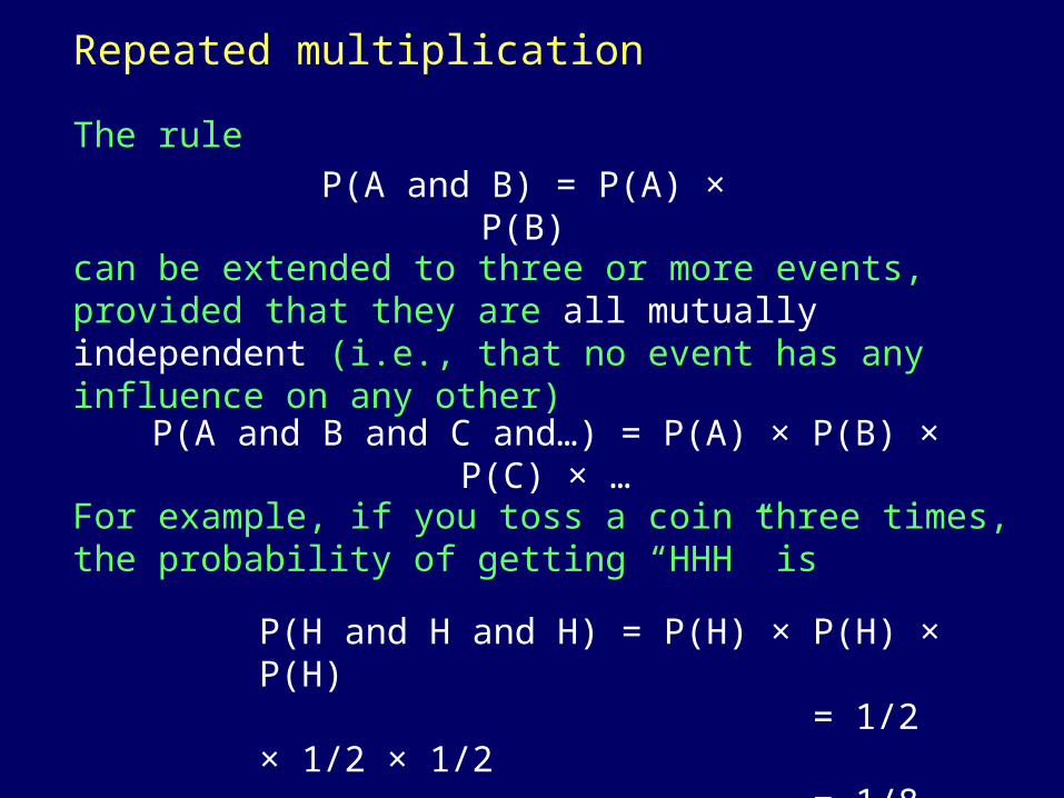
Repeated multiplication

The rule

can be extended to three or more events, provided that they are all mutually independent (i.e., that no event has any influence on any other)

P(A and B) = P(A) × P(B)

P(A and B and C and…) = P(A) × P(B) × P(C) × …

For example, if you toss a coin three times, the probability of getting “HHH” is

P(H and H and H) = P(H) × P(H) × P(H) = 1/2 × 1/2 × 1/2 = 1/8

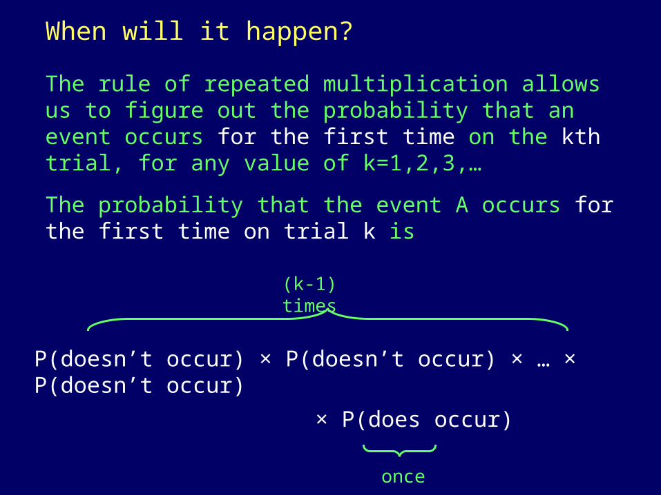
When will it happen?

The rule of repeated multiplication allows us to figure out the probability that an event occurs for the first time on the kth trial, for any value of k=1,2,3,…

The probability that the event A occurs for the first time on trial k is

P(doesn’t occur) × P(doesn’t occur) × … × P(doesn’t occur)

× P(does occur)

(k-1) times

once

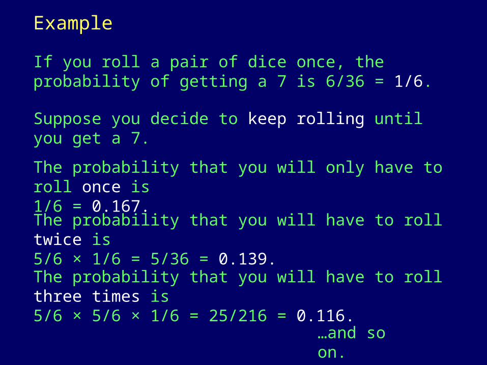
Example

If you roll a pair of dice once, the probability of getting a 7 is 6/36 = 1/6.

Suppose you decide to keep rolling until you get a 7.

The probability that you will only have to roll once is1/6 = 0.167.The probability that you will have to roll twice is5/6 × 1/6 = 5/36 = 0.139.

The probability that you will have to roll three times is5/6 × 5/6 × 1/6 = 25/216 = 0.116.

…and so on.

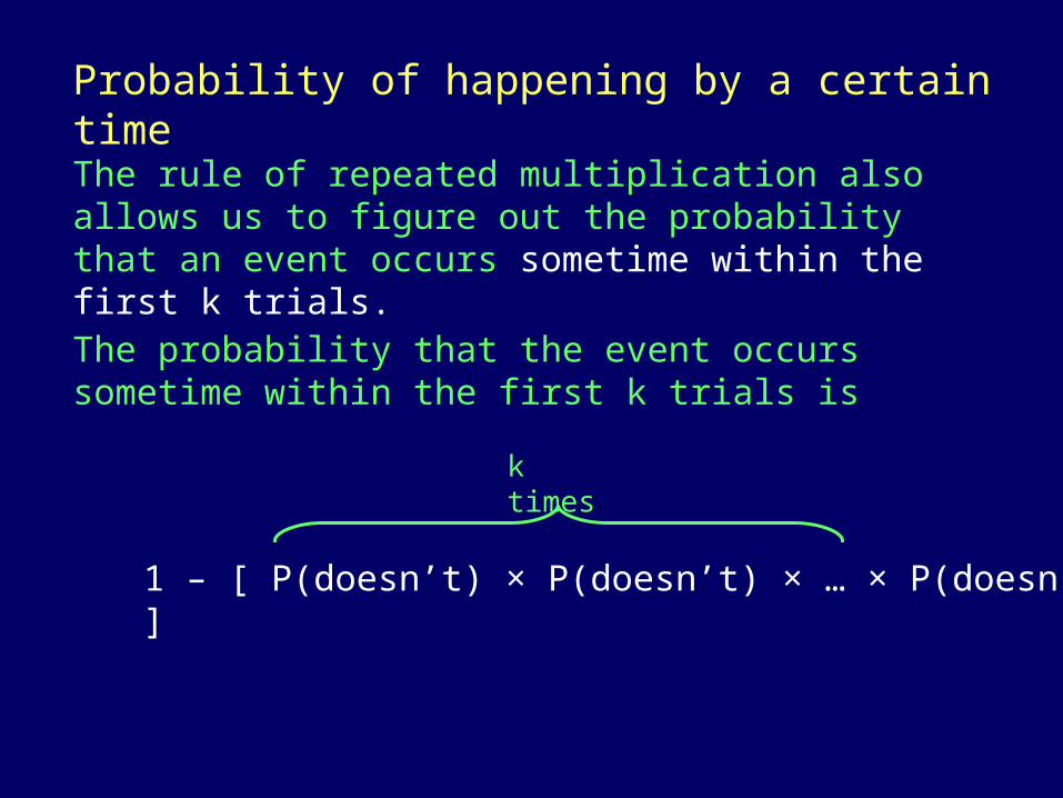
Probability of happening by a certain time

The rule of repeated multiplication also allows us to figure out the probability that an event occurs sometime within the first k trials.

The probability that the event occurs sometime within the first k trials is

1 – [ P(doesn’t) × P(doesn’t) × … × P(doesn’t) ]

k times

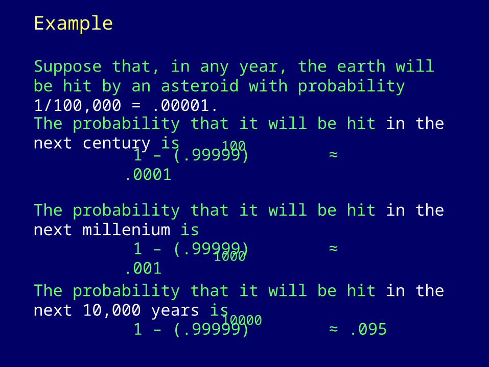
Example

Suppose that, in any year, the earth will be hit by an asteroid with probability 1/100,000 = .00001.

The probability that it will be hit in the next century is

1 – (.99999) ≈ .0001 100

The probability that it will be hit in the next millenium is

1 – (.99999) ≈ .001 1000

The probability that it will be hit in the next 10,000 years is

1 – (.99999) ≈ .095 10000

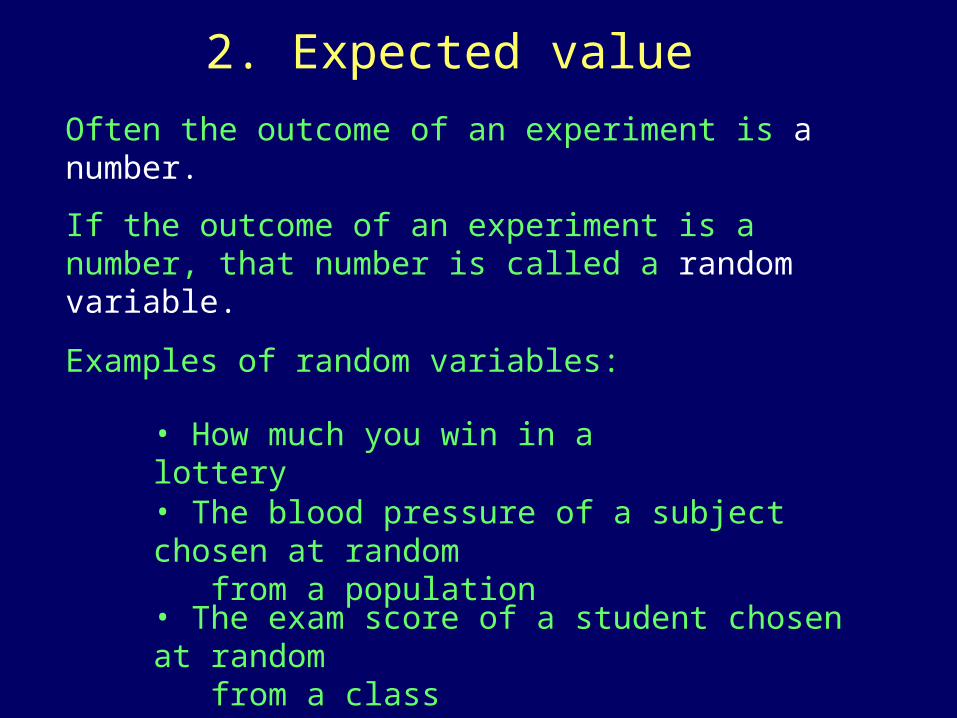
2. Expected value

Often the outcome of an experiment is a number.

If the outcome of an experiment is a number, that number is called a random variable.

Examples of random variables:

• How much you win in a lottery• The blood pressure of a subject chosen at random from a population• The exam score of a student chosen at random from a class

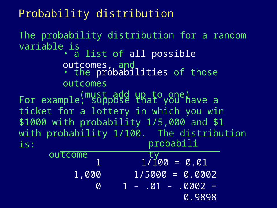
Probability distribution

The probability distribution for a random variable is

1,000 1/5000 = 0.00021 1/100 = 0.01

0 1 – .01 – .0002 = 0.9898

outcome

probability

• a list of all possible outcomes, and

• the probabilities of those outcomes (must add up to one)

For example, suppose that you have a ticket for a lottery in which you win $1000 with probability 1/5,000 and $1 with probability 1/100. The distribution is:

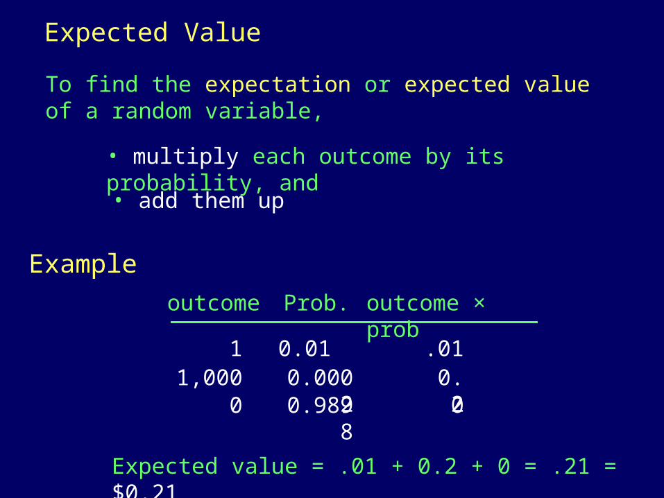
Expected Value

To find the expectation or expected value of a random variable,

• multiply each outcome by its probability, and• add them up

1,000 0.0002

1 0.01

0 0.9898

outcome Prob.

Expected value = .01 + 0.2 + 0 = .21 = $0.21

0.2.01

0

outcome × prob

Example

Interpretation of Expected Value

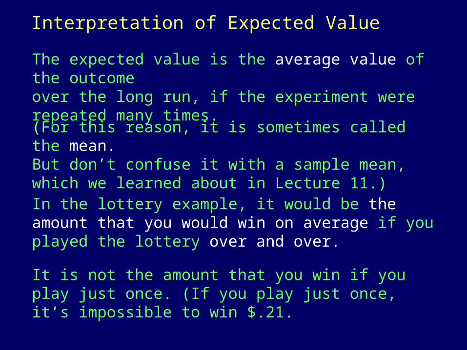
The expected value is the average value of the outcomeover the long run, if the experiment were repeated many times.(For this reason, it is sometimes called the mean.But don’t confuse it with a sample mean, which we learned about in Lecture 11.)

In the lottery example, it would be the amount that you would win on average if you played the lottery over and over.

It is not the amount that you win if you play just once. (If you play just once, it’s impossible to win $.21.

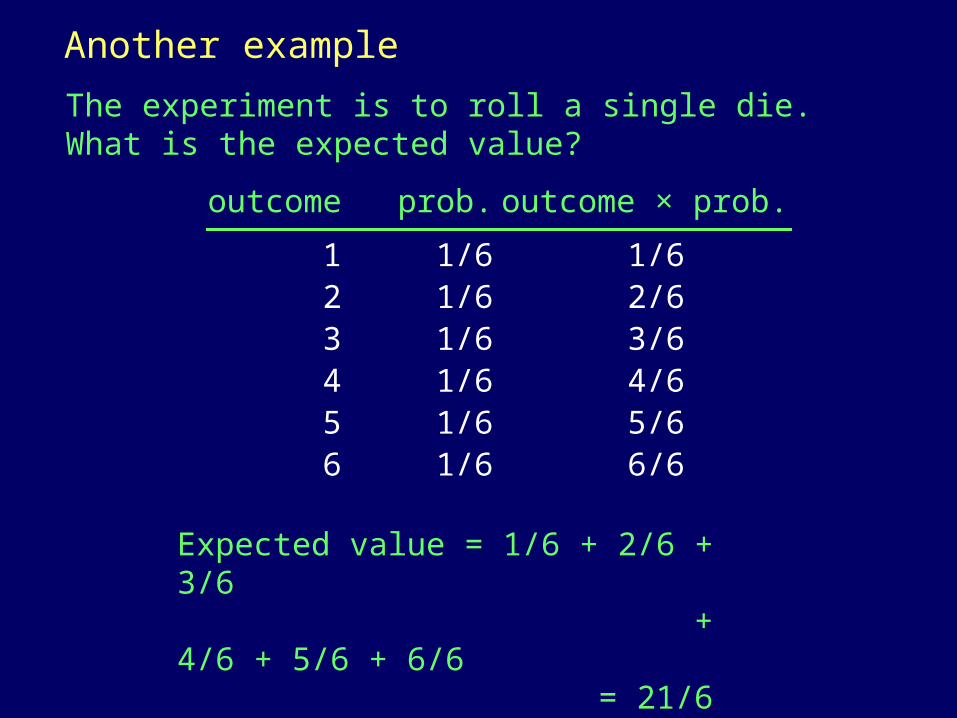
Another example

The experiment is to roll a single die. What is the expected value?

12

outcome

3456

1/61/6

prob.

1/61/61/61/6

1/62/63/64/65/66/6

Expected value = 1/6 + 2/6 + 3/6 + 4/6 + 5/6 + 6/6 = 21/6 = 3.5

outcome × prob.