Plenary Data Analysis SessionPSI Conference Bristol 2006

John MatthewsSchool of Mathematics and StatisticsUniversity of Newcastle upon Tyne

Five Period Crossover volunteer study

Active treatments, A to F – six doses of a new compound

Two control treatments, c1, c2, namely

a positive control S - a standard treatment already on the market

a negative control P - a placebo with zero dose of the active compound

Alternating study, two cohorts, each of 10 volunteers

A to F are increasing doses dj in g

Exact doses not taken into account in analysis but doses must escalate

Contrasts dj - ci of equal and primary interest: i = 1,2 and j = 1,…,6

A B C D E F

10 30 60 150 250 400

Within each period, data (FEV1) collected at baseline and at six times post administration

Main interest is in response at 12 hours

One volunteer withdrew after three periods (missed P and F), otherwise data complete

Substantial washout – no carryover, ?period effect?

Quick and thoughtless analysis

Fixed subjects effects Period effect No period to period baseline

ANOVA table

Df Sum Sq Mean Sq F value Pr(>F) factor(subject) 19 50.672 2.667 115.4127 <2.e-16 factor(period) 4 0.120 0.030 1.2969 0.28017 factor(Rx) 7 0.467 0.067 2.8880 0.01067 *

Residuals 67 1.548 0.023

No strong evidence of period effect Some treatment effect – largely because

of difference between +ve and –ve controls

Mean effects

DoseMean Difference (l) from

negative control(baseline as covariate)

SE P

10 -0.087 -0.077 0.069 0.062 0.21 0.22

30 -0.052 -0.045 0.070 0.063 0.46 0.48

60 -0.039 -0.009 0.067 0.061 0.57 0.88

150 -0.046 -0.034 0.068 0.061 0.50 0.58

250 -0.029 -0.029 0.070 0.063 0.68 0.65

400 -0.043 -0.058 0.074 0.067 0.56 0.39

S 0.125 0.158 0.049 0.044 0.013 0.0008

Design

V’rs Cohort 1 V’rs Cohort 2

1,2 P A S C E 11,12 P B S D F

3,4 S A C E P 13,14 S B D F P

5,6 A C P E S 15, 16 B D P F S

7,8 A P C S E 17, 18 B P D S F

9.10 A S C P E 19,20 B S D P F

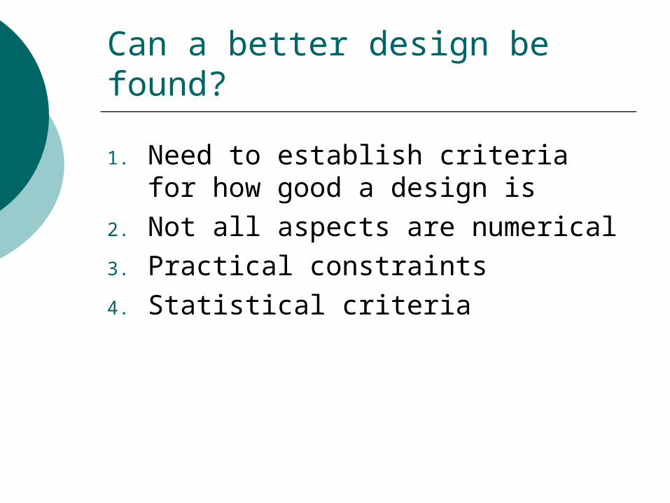
Can a better design be found?

1. Need to establish criteria for how good a design is

2. Not all aspects are numerical3. Practical constraints4. Statistical criteria

Practical constraints

Doses must escalate Don’t start too high Dose increments should not be too

large Two cohorts - cohort 2 investigated

while cohort 1 rests. Study to finish in 3/12

Statistical criteria

Model can be written as

Hence

where

NuisPeriodVolun.Rx ]||[)(E

XXXXy

RxPeriodVolun.Rx ])}|([{)ˆ(Inf XXXIXC T

TT AAAAA )()(

Variance of contrasts

Want to consider variance of estimate of This might be thought to be C-1 but C is

singular Therefore use g-inverse C-

C- is not unique but If A is a c t matrix of contrasts of interest

then dispersion of contrasts, AC-A, is well defined

(need rank(C)=7=t-1 if all contrasts to be estimable)

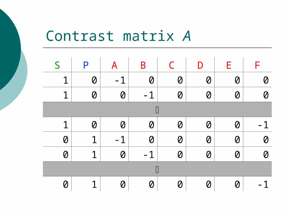
Contrast matrix A

S P A B C D E F

1 0 -1 0 0 0 0 0

1 0 0 -1 0 0 0 0

1 0 0 0 0 0 0 -1

0 1 -1 0 0 0 0 0

0 1 0 -1 0 0 0 0

0 1 0 0 0 0 0 -1

Statistical Criterion

If all else is equal, we prefer a design with lower mean variance for a contrast of interest, i.e. minimise

trace(AC-A)

Might want to minimise max{(AC-A)ii} but this is not pursued here

Practical improvements to design

Split doses into {A,C,E} and {B,D,F} to permit alternating design

Also ensures that dose increments are not large

Given doses must escalate there is little room for use of different designs

Flexibility about when controls given Once these are chosen, sequences are

defined

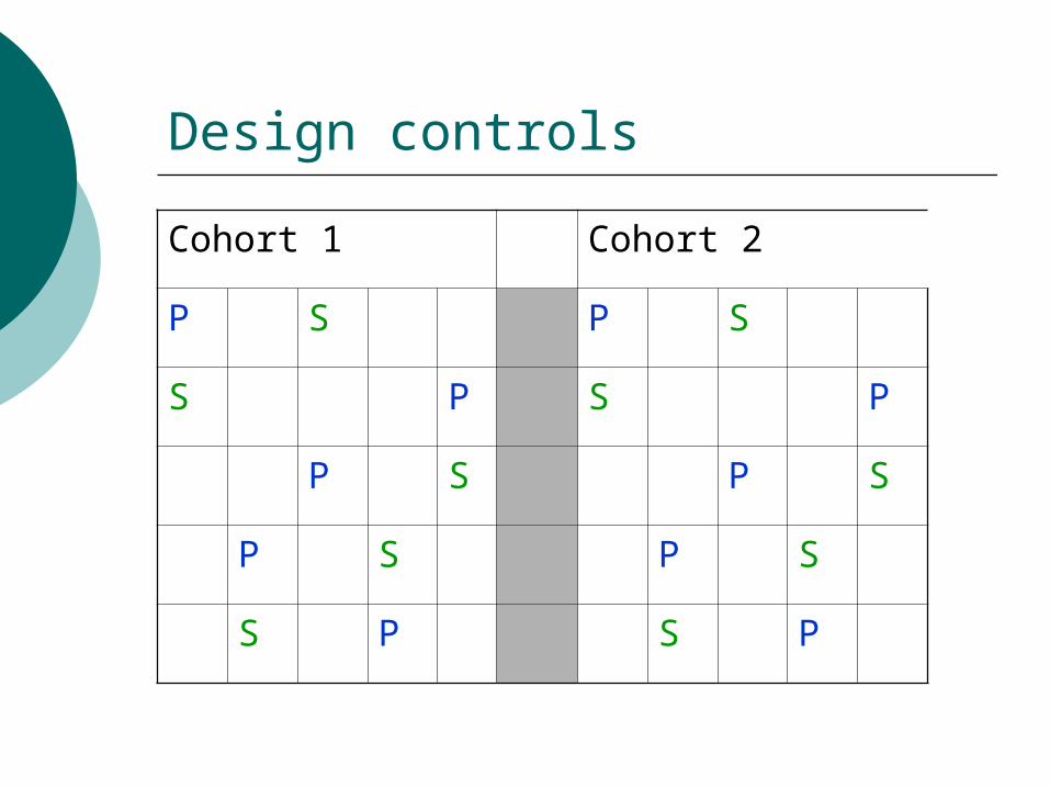
Design controls

Cohort 1 Cohort 2

P S P S

S P S P

P S P S

P S P S

S P S P

Control disposition

Same pattern in two cohorts P before S in 12 volunteers trace(AC-A)=2.429 There are 5C2 = 10 different

unordered pairs of places in a sequence

Allowing for order there are twenty possible sequences for each cohort

Possible control sequences

P S

P S

P S

P S

P S

P S

P S

P S

P S

P S

Type ‘PS’ sequences

Further 10 sequences with S preceding P, type ‘SP’ sequences

Fill in gaps with either {A,C,E} or {B,D,F}

Allocate {A,C,E} to 10 sequences and {B,D,F} to remainder – allows alternation and close to balance on volunteers

Allocation method 1

P S

P S

P S

P S

P S

P S

P S

P S

P S

P S

40 possible sequences

10 with {A,C,E} in sequences shown

10 with {A,C,E} and Type ‘SP’ sequences

20 as above but with {B,D,F} not {A,C,E}

Choose random 20 from these 40. Perhaps search for a ‘good’ set

Method 1

For original designtrace(AC-A)=2.429

Method 1 ensures no particular degree of balance Optimal row-column designs are uniform on

periods and subjects, i.e. each treatment appears equally often on each volunteer and in each period

Cannot achieve this but can we get ‘close’? If we achieve a certain balance on volunteers,

‘closeness’ can be measured by treatment by period incidence matrix

Example of a Treatment Period Incidence Matrix

P S A B C D E F

4 4 a a 0 0 0 0

4 4 b b c c 0 0

4 4 d d e e f f

4 4 0 0 c c b b

4 4 0 0 0 0 a a

Treatment Period Incidence Matrix for original design

P S A B C D E F

4 4 6 6 0 0 0 0

4 4 4 4 2 2 0 0

4 4 0 0 6 6 0 0

4 4 0 0 2 2 4 4

4 4 0 0 0 0 6 6

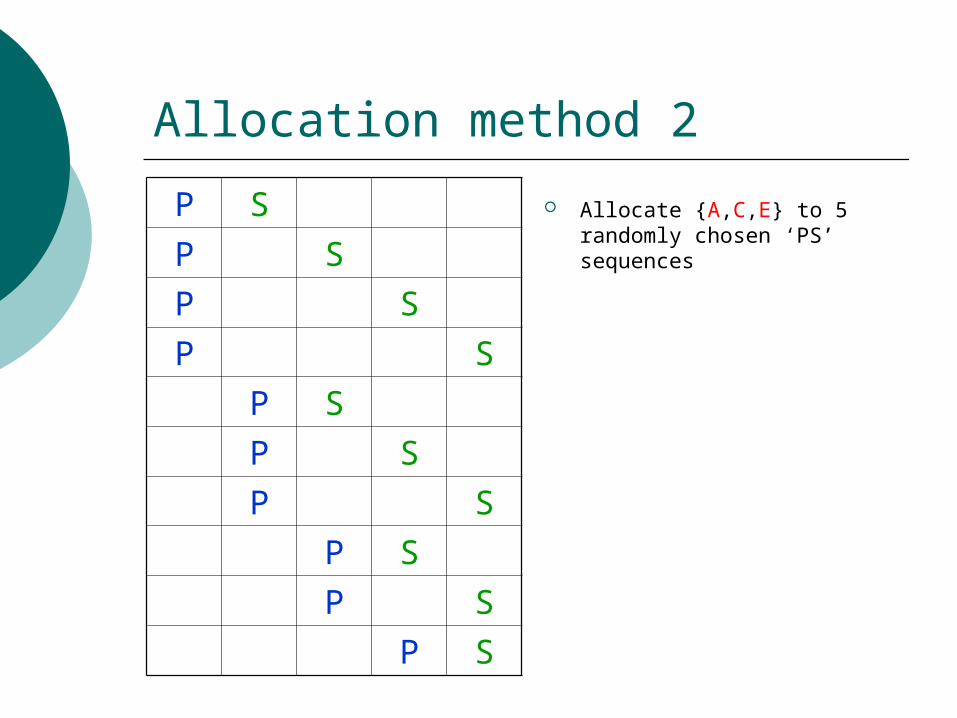
Allocation method 2

P S

P S

P S

P S

P S

P S

P S

P S

P S

P S

Allocate {A,C,E} to 5 randomly chosen ‘PS’ sequences

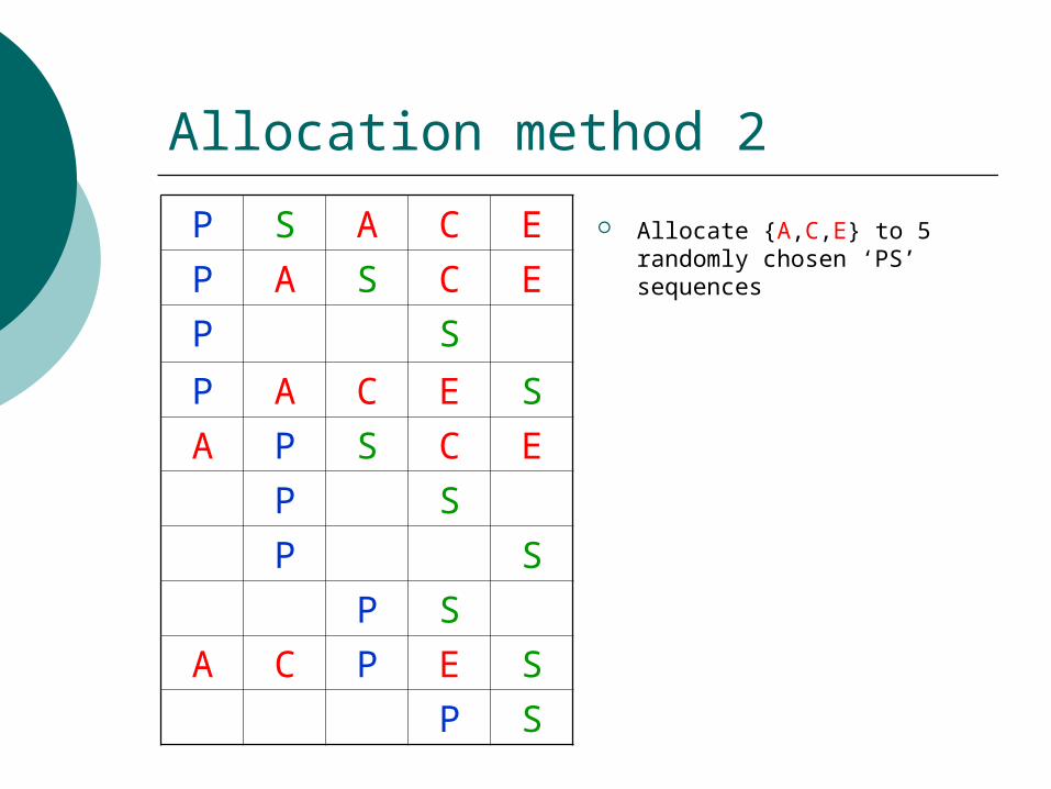
Allocation method 2

P S A C E

P A S C E

P S

P A C E S

A P S C E

P S

P S

P S

A C P E S

P S

Allocate {A,C,E} to 5 randomly chosen ‘PS’ sequences

Allocation method 2

P S A C E

P A S C E

P S

P A C E S

A P S C E

P S

P S

P S

A C P E S

P S

Allocate {A,C,E} to 5 randomly chosen ‘PS’ sequences

Allocate {B,D,F} other 5 ‘PS’ sequences

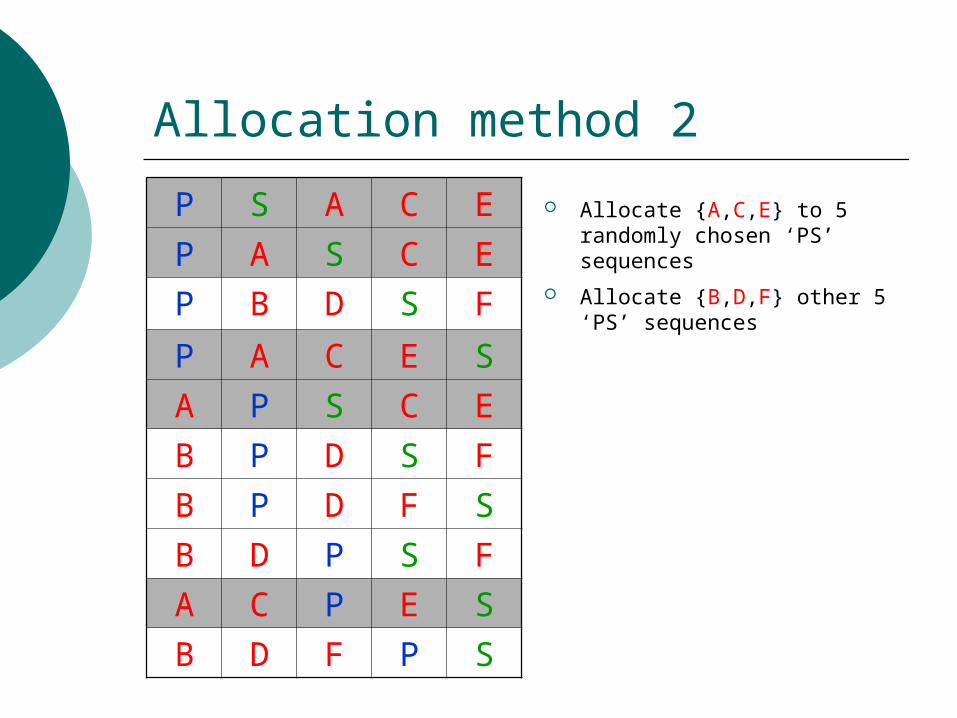
Allocation method 2

P S A C E

P A S C E

P B D S F

P A C E S

A P S C E

B P D S F

B P D F S

B D P S F

A C P E S

B D F P S

Allocate {A,C,E} to 5 randomly chosen ‘PS’ sequences

Allocate {B,D,F} other 5 ‘PS’ sequences

Allocation method 2

P S A C E

P A S C E

P B D S F

P A C E S

A P S C E

B P D S F

B P D F S

B D P S F

A C P E S

B D F P S

Allocate {A,C,E} to 5 randomly chosen ‘PS’ sequences

Allocate {B,D,F} other 5 ‘PS’ sequences

This gives full replication of ‘PS’ sequences

Allocate {A,C,E} to the 5 ‘SP’ sequences analogous to the ‘PS’ sequences just allocated to {B,D,F}

Allocate {B,D,F} to remaining ‘SP’ sequences

Gives balance over periods of two sets of doses

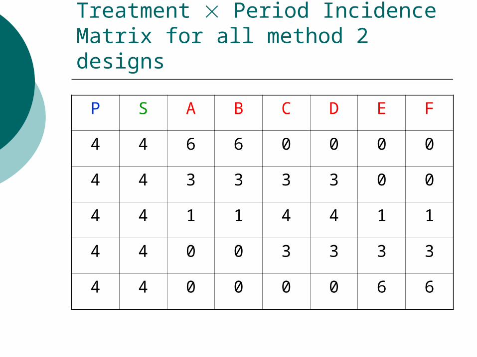
Treatment Period Incidence Matrix for all method 2 designs

P S A B C D E F

4 4 6 6 0 0 0 0

4 4 3 3 3 3 0 0

4 4 1 1 4 4 1 1

4 4 0 0 3 3 3 3

4 4 0 0 0 0 6 6

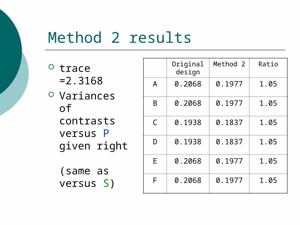
Method 2 results

trace =2.3168

Variances of contrasts versus P given right

(same as versus S)

Original design

Method 2 Ratio

A 0.2068 0.1977 1.05

B 0.2068 0.1977 1.05

C 0.1938 0.1837 1.05

D 0.1938 0.1837 1.05

E 0.2068 0.1977 1.05

F 0.2068 0.1977 1.05

Further method

Method 2 imposes balance but does not allow duplication of sequences

May be merit in allowing this

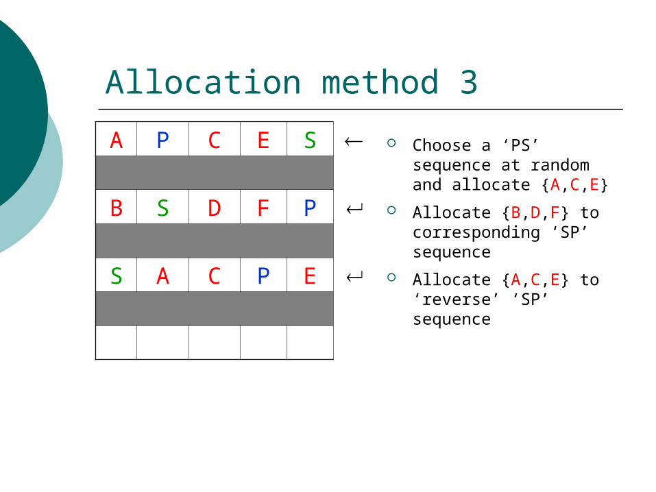
Allocation method 3

A P C E S Choose a ‘PS’ sequence at random and allocate {A,C,E}

Allocation method 3

A P C E S

B S D F P

Choose a ‘PS’ sequence at random and allocate {A,C,E}

Allocate {B,D,F} to corresponding ‘SP’ sequence

Allocation method 3

A P C E S

B S D F P

S A C P E

Choose a ‘PS’ sequence at random and allocate {A,C,E}

Allocate {B,D,F} to corresponding ‘SP’ sequence

Allocate {A,C,E} to ‘reverse’ ‘SP’ sequence

Allocation method 3

A P C E S

B S D F P

S A C P E

P B D S F

Choose a ‘PS’ sequence at random and allocate {A,C,E}

Allocate {B,D,F} to corresponding ‘SP’ sequence

Allocate {A,C,E} ‘reverse’ ‘SP’ sequence

and {B,D,F} to the analogous ‘PS’ sequence

Allocation method 3

A P C E S

B S D F P

S A C P E

P B D S F

Choose a ‘PS’ sequence at random and allocate {A,C,E}

Allocate {B,D,F} to corresponding ‘SP’ sequence

Allocate {A,C,E} ‘reverse’ ‘SP’ sequence

and {B,D,F} to the analogous ‘PS’ sequence

This allocates 4 volunteers – repeat a further 4 times, sampling with replacement at first step

Allocation method 3: chosen design

A C E P S 3

P A C S E 1

A C P E S 1

plus other sequences as in

method 3

trace =2.262

Treatment Period Incidence Matrix for method 3 design

P S A B C D E F

5 5 5 5 0 0 0 0

4 4 2 2 4 4 0 0

2 2 3 3 2 2 3 3

4 4 0 0 4 4 2 2

5 5 0 0 0 0 5 5

Method 3 results

trace =2.262 Variances of

contrasts versus P given right

(same as versus S)

Original design

Method 3 Ratio

A 0.2068 0.1885 1.10

B 0.2068 0.1885 1.10

C 0.1938 0.1883 1.03

D 0.1938 0.1883 1.03

E 0.2068 0.1885 1.10

F 0.2068 0.1885 1.10

Conclusions

Little room for manoeuvre in design of dose-escalating studies

Positioning of controls is about limit Nevertheless worth doing – proposed

change equivalent to 10% reduction in variance at no cost

Work to be done to extend existing work on comparison with multiple controls to allow for other constraints