P.Lewis (1) Gomez-Dans, J.(1), Kaminski, T.(2); Settle, J.(3), Quaife, T.(3), Gobron, N.(4), Styles, J.

(5), Berger, M. (6)

Data Assimilation of Sentinel-2 Observations: Preliminary results from EO-LDAS and Outlook

(1) UCL and NCEO, (2) FastOpt, (3) University of Reading and NCEO (4) European Commission, DG Joint Research Centre (5) Assimila Ltd., (6) ESA ESRIN, Science

Strategy, Coordination and Planning Office (EOP-SA),

+FSU Jena (field data)

EO-LDAS

• ESA STSE project

• prototype Earth Observation Data Assimilation System

• Software soon to be released: python package

• gain experience with using DA with EO data

• Variational system

• Includes interface to the canopy Radiative Transfer model: semi-discrete (Gobron et al.)• + soil & leaf spectral

• with associated adjoint code

The remote sensing problem

• Context here: vegetation canopies

• Infer vegetation properties from radiometry

• E.g. LAI, chlorophyll, water

• Test/drive models e.g. biogeochem. for C flux, crop models etc.

• Historically

• Vegetation indices

• Data transforms to maximise sensitivity to target variable (e.g. LAI)

• Empirical or model-based relationships

• Model ‘inversion’

• RT model predictions of measurements y as function of state x

• LUT/ANN mapping of inverse function

Issues with inversion

• Poor or no treatment of uncertainty

• Problem mostly ill-conditioned

• Not enough information to solve for all terms

• E.g. RT model state:

• Assume some terms ‘known’

• Better to specify knowledge as explicit constraint

• With associated uncertainty

LAI Leaf inclination distribution

Leaf chlorophyll

Leaf water Leaf dry matter

Soil brightness

Soil water

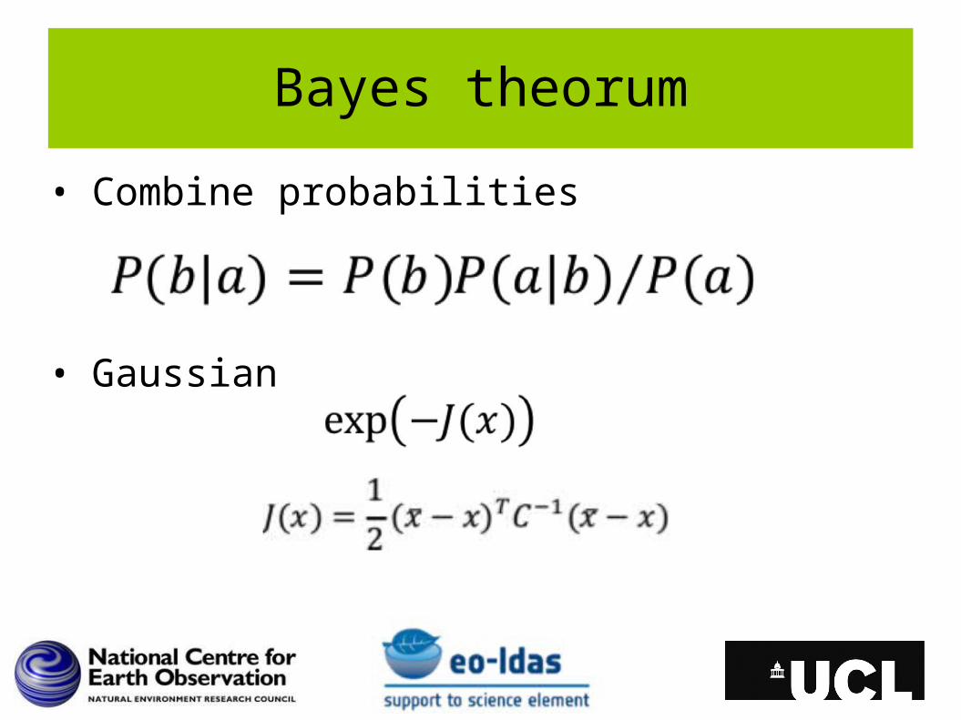
Bayes theorum

• Combine probabilities

• Gaussian

Combine prior and observation

Optimal (ML) estimate for x at max(exp(j))

So min(J)

Recognise J as ‘cost fn’

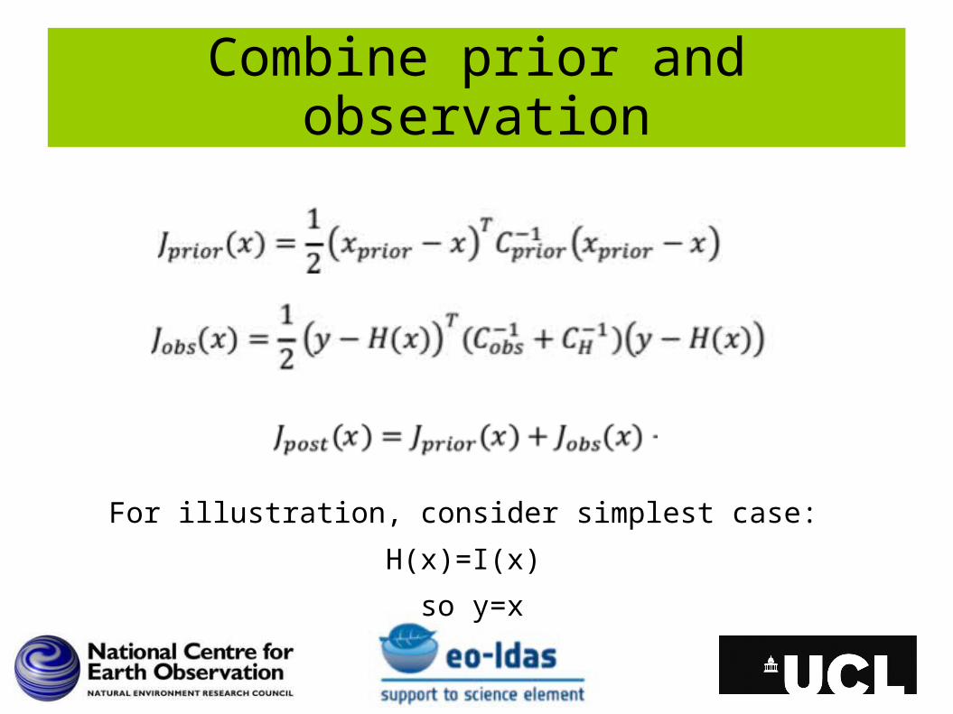
Combine prior and observation

For illustration, consider simplest case:

H(x)=I(x)

so y=x

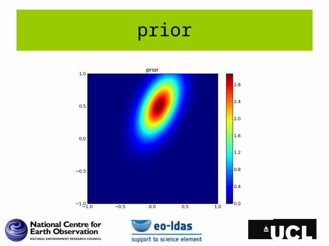
prior

observation

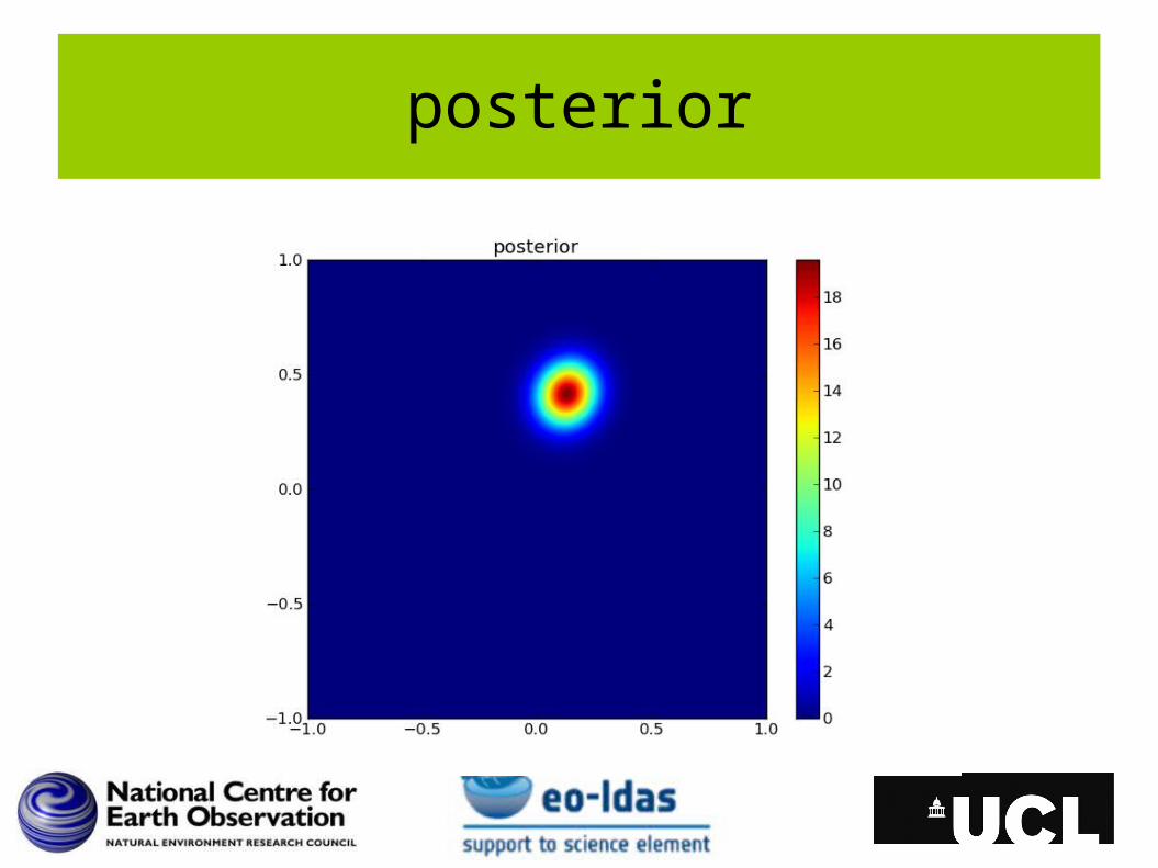
posterior

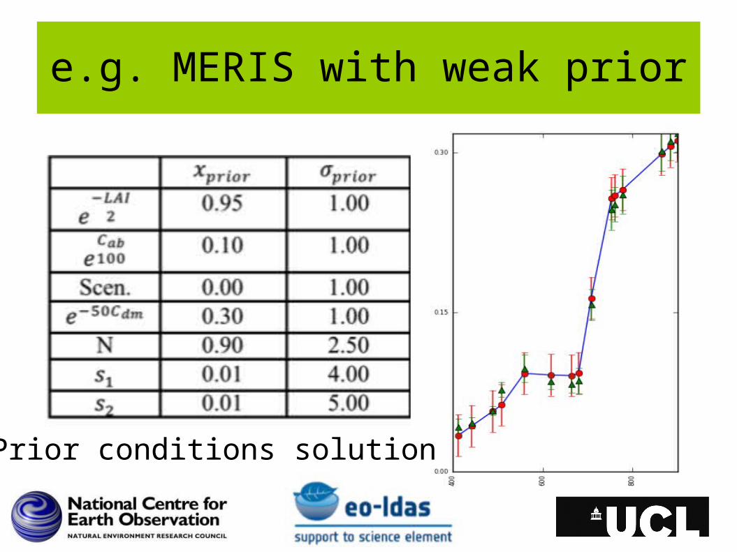
e.g. MERIS with weak prior

Prior conditions solution

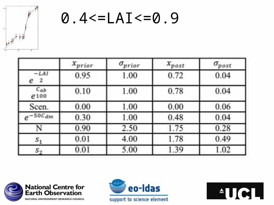
0.4<=LAI<=0.9

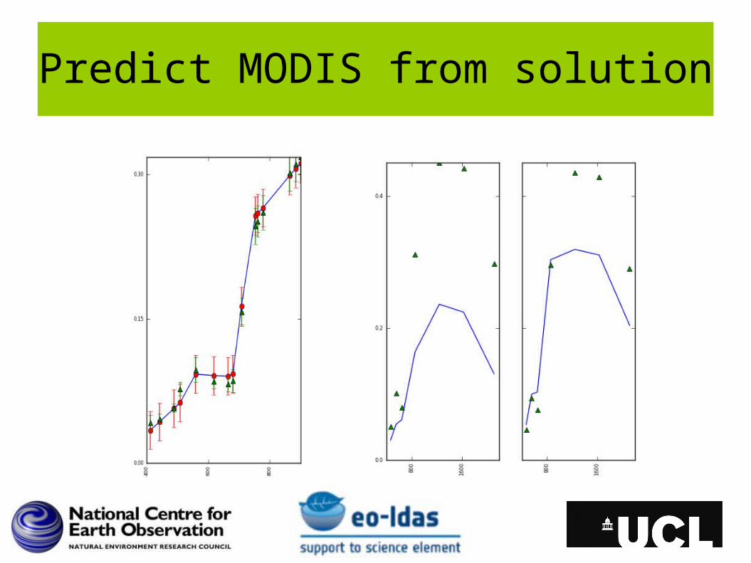
Predict MODIS from solution

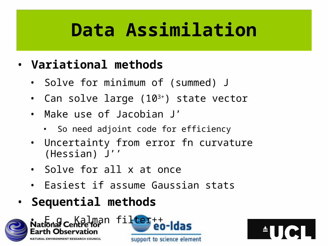
Data Assimilation

• Variational methods

• Solve for minimum of (summed) J

• Can solve large (103+) state vector

• Make use of Jacobian J’

• So need adjoint code for efficiency

• Uncertainty from error fn curvature (Hessian) J’’

• Solve for all x at once

• Easiest if assume Gaussian stats

• Sequential methods

• E.g. Kalman filter++

Elements of a DA system

• State vector x

• Observations y

• Prior constraint

• Process model Q(x)

• Obs constraint with y=H(x)

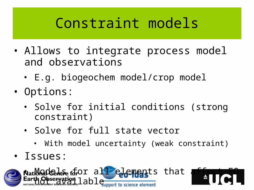
Constraint models

• Allows to integrate process model and observations

• E.g. biogeochem model/crop model

• Options:

• Solve for initial conditions (strong constraint)

• Solve for full state vector• With model uncertainty (weak constraint)

• Issues:

• Models for all elements that affect EO not available

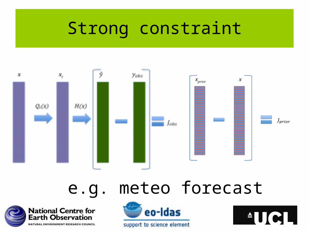
Strong constraint

e.g. meteo forecast

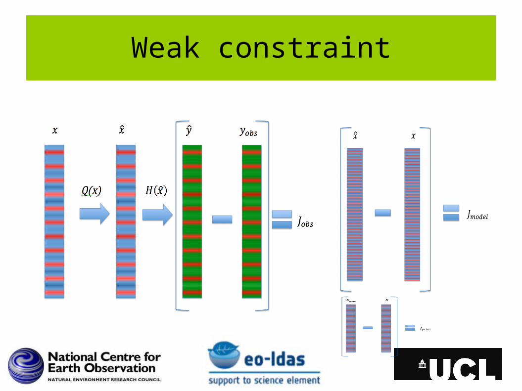
Weak constraint

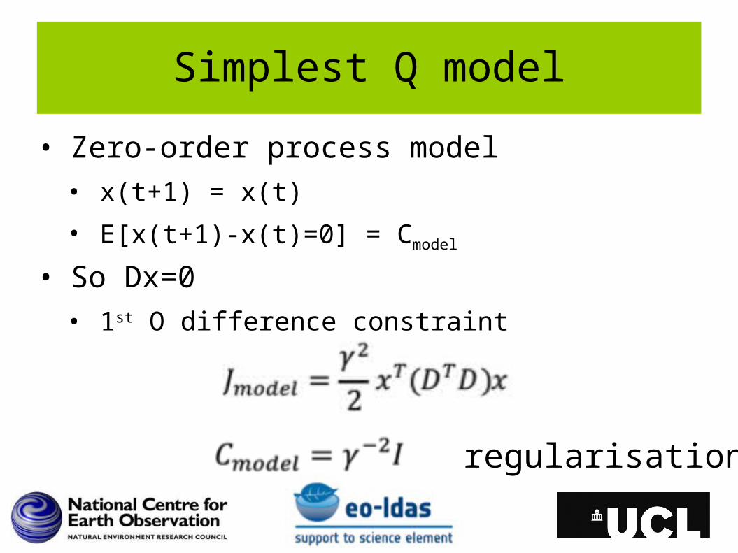
Simplest Q model

• Zero-order process model

• x(t+1) = x(t)

• E[x(t+1)-x(t)=0] = Cmodel

• So Dx=0

• 1st O difference constraint

regularisation

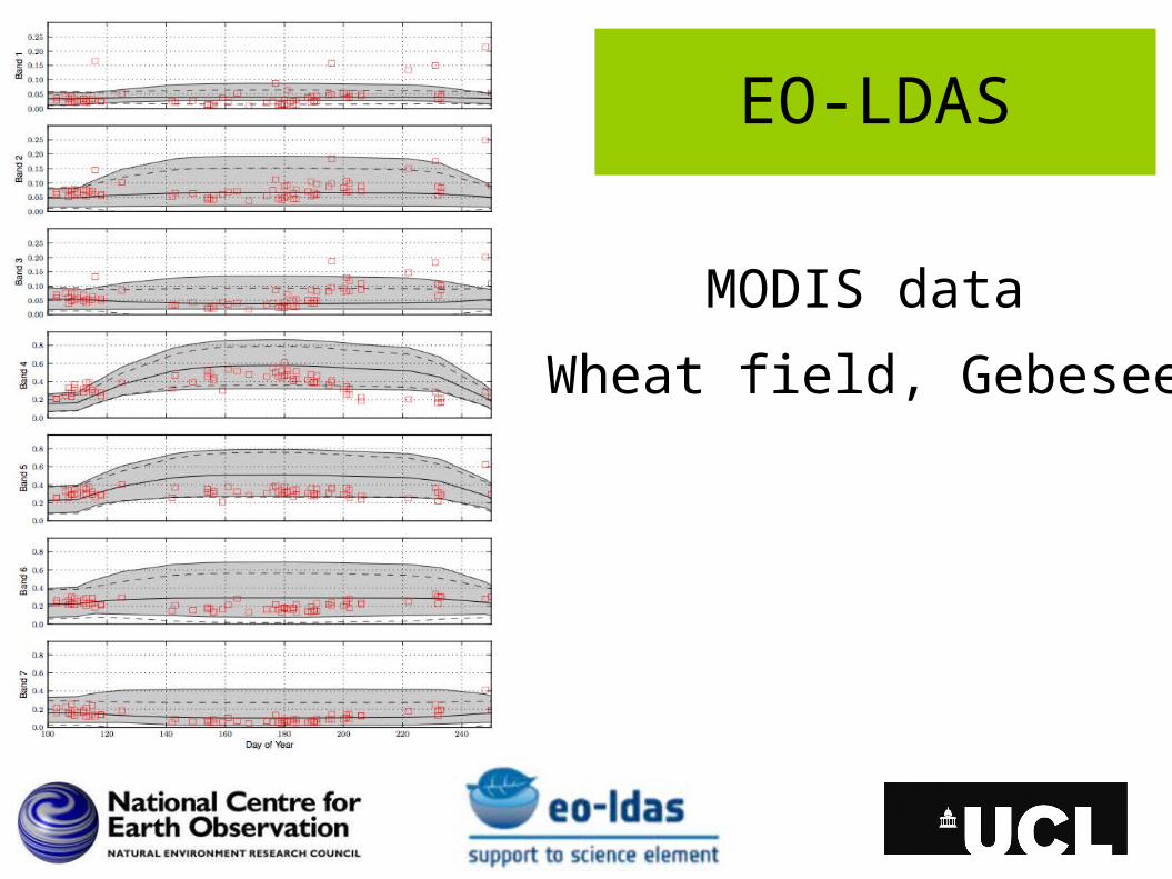
EO-LDAS

MODIS data

Wheat field, Gebesee

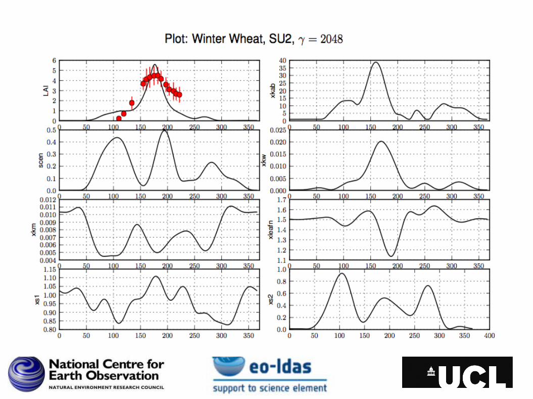
MODIS results

• Slight over-smoothed

• But viable LAI

• But demonstrate ability to solve for all (8 here) vegetation state parameters

• For each day of year = 8x365 ~= 3000

• Using only simple regularisation model

• 2nd difference here

Sentinel-2 MSI

• Synthetic experiment

• See Lewis et al. (2012) RSE

• 2 scenarios

• Full (5 day) coverage

• Cloudy (50%) coverage

• Assume temporal trajectories

• Green lines in plots

• Solve for vegetation state

• For each sample day (loose prior only)

• With prior + D1 & D2 regularisation models

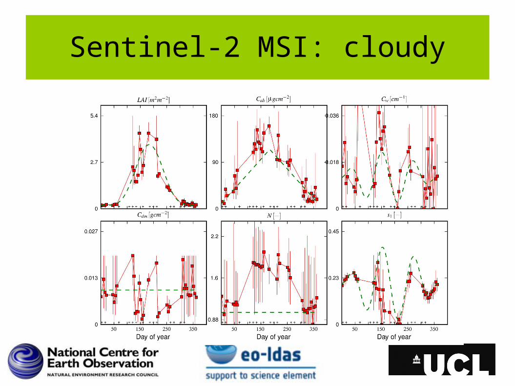
Sentinel-2 MSI: cloudy

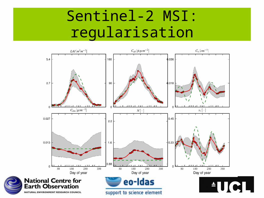
Sentinel-2 MSI: regularisation

Sentinel-2 MSI

• Viable results for MSI with prior

• But quite large uncertainties

• DA with regularisation model

• Reduce uncertainty by ~2 on average

• Solve for all days

• Speed bottleneck for full RT model

• Replace by GP emulation models

• Same for process models?

Outlook

• DA framework appropriate way to estimate vegetation state from EO

• Priors express certainty in expectations

• Rather than simply assuming terms constant

• Regularisation methods allow estimation of full state vector

• If no other process model available

• Or if purpose is to test process model

• Framework can integrate any process models

• E.g. biogeochem models for C flux estimation

• E.g. crop growth

• Framework can be applied to space as well as time

• Route for multi-scale sensor integration

EO-LDAS

• Project website

http://www.assimila.eu/eoldas/

• Software tutorial

http://www2.geog.ucl.ac.uk/~plewis/eoldas

• Software release soon

• New ESA DA project

• Integrate SVAT/vegetation dynamics models

• More observation operators:

• Passive microwave

Thank you