PLoS Comput Biol 2014 Serkh - Schedules of Light Exposure to Correct Circadian Misalignment

7/18/2019 PLoS Comput Biol 2014 Serkh - Schedules of Light Exposure to Correct Circadian Misalignment

http://slidepdf.com/reader/full/plos-comput-biol-2014-serkh-schedules-of-light-exposure-to-correct-circadian 1/14

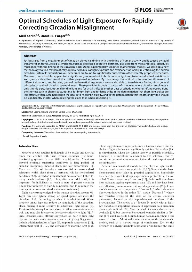
Optimal Schedules of Light Exposure for RapidlyCorrecting Circadian Misalignment

Kirill Serkh1,2, Daniel B. Forger2,3*

1 Department of Applied Mathematics, Graduate School of Arts & Sciences, Yale University, New Haven, Connecticut, United States of America, 2 Department of

Mathematics, University of Michigan, Ann Arbor, Michigan, United States of America, 3 Computational Medicine and Bioinformatics, University of Michigan, Ann Arbor,

Michigan, United States of America

Abstract

Jet lag arises from a misalignment of circadian biological timing with the timing of human activity, and is caused by rapidtransmeridian travel. Jet lag’s symptoms, such as depressed cognitive alertness, also arise from work and social schedulesmisaligned with the timing of the circadian clock. Using experimentally validated mathematical models, we develop a newmethodology to find mathematically optimal schedules of light exposure and avoidance for rapidly re-entraining the humancircadian system. In simulations, our schedules are found to significantly outperform other recently proposed schedules.Moreover, our schedules appear to be significantly more robust to both noise in light and to inter-individual variations inendogenous circadian period than other proposed schedules. By comparing the optimal schedules for thousands of different situations, and by using general mathematical arguments, we are also able to translate our findings into generalprinciples of optimal circadian re-entrainment. These principles include: 1) a class of schedules where circadian amplitude isonly slightly perturbed, optimal for dim light and for small shifts 2) another class of schedules where shifting occurs alongthe shortest path in phase-space, optimal for bright light and for large shifts 3) the determination that short light pulses are

less effective than sustained light if the goal is to re-entrain quickly, and 4) the determination that length of daytime shouldbe significantly shorter when delaying the clock than when advancing it.

doi:10.1371/journal.pcbi.1003523

Editor: Olaf Sporns, Indiana University, United States of America

Received September 23, 2013; Accepted January 29, 2014; Published

Copyright: 2014 Serkh, Forger. This is an open-access article distributed under the terms of the Creative Commons Attribution License, which permitsunrestricted use, distribution, and reproduction in any medium, provided the original author and source are credited.

Funding: This work was supported by AFOSR grant FA9550-11-1-0165 and internal funds from the University of Michigan. The funders had no role in studydesign, data collection and analysis, decision to publish, or preparation of the manuscript.

Competing Interests: The authors have declared that no competing interests exist.

* E-mail: [email protected].

Introduction

Modern society requires individuals to be awake and alert at

times that conflict with their internal circadian ( ,24-hour)

timekeeping systems. In year 2012 over 60 million Americans

traveled overseas, subjecting themselves to long periods of

circadian mistiming, impaired sleep, and low performance [1].

Over one fifth of American workers follow non-standard

schedules, which place them at increased risk for sleep-related

accidents [2,3]. Circadian misalignment has also been linked to

many health problems [4,5]. Thus, after a schedule shift, it is

important for individuals to reach a state of proper circadian

timing (entrainment) as quickly as possible, and to minimize the

time spent between entrained states (re-entrainment).

Light is the strongest signal to the human circadian system [6].

Light can slow (phase delay), or speed (phase advance) the

circadian clock, depending on when it is administered. When

properly timed, light can reduce the amplitude of the circadian

clock, making it more sensitive to subsequent light signals [7].

Previous light history has been shown to affect re-entrainment as

well, and may also increase or decrease sensitivity to light [8]. A

large literature exists offering suggestions on how to time light

exposure to quicken re-entrainment and avoid jet lag. Suggestions

include additional pulses of light [9], amplitude suppression [10],

intermittent light [11,12], and avoidance of morning light [13].

These suggestions are important, since it has been shown that the

choice of light schedule can significantly quicken [14] or slow [15]

re-entrainment. Given the infinite variety of possible schedules,

however, it is unrealistic to attempt to find schedules that re-

entrain in the minimum amount of time through experimental

methods alone.

Accurate mathematical models for the effect of light on the

human circadian system are available [16,17]. Several studies have

demonstrated their value in practical applications. Specifically

they have been used to design experimental protocols i.e. the so-

called ‘‘forced desynchony’’ protocol [18]; their predictions have

been validated against experimental data [19]; and they have been

used effectively in numerous real-world applications [20]. These

models contain two components: ‘‘Process L,’’ which simulates

phototransduction in the retina [21], and a ‘‘Process P,’’ whose

two variables represent the state of the central circadian

pacemaker, located in the suprachiasmatic nucleus of the

hypothalamus. The choice of a ‘‘Process P’’ model with at least

two variables is important, because it represents both circadian

phase and amplitude [22]. More detailed biochemical models are

available [23], but these can be reduced to models similar to [16]

and [17], and have yet to be fit to human data, making them a less

attractive choice. Additionally, many features of the biochemical

models, such as a narrow range of entrainment [24] or the

presence of a sharp threshold separating orthodromic (the same

PLOS Computational Biology | www.ploscompbiol.org 1 April 2014 | Volume 10 | Issue 4 | e1003523

April 10, 2014

Citation: Serkh K, Forger DB (2014) Optimal Schedules of Light Exposure for Rapidly Correcting Circadian Misalignment. PLoS Comput Biol 10(4): e1003523.

http://creativecommons.org/licenses/by/4.0/

http://crossmark.crossref.org/dialog/?doi=10.1371/journal.pcbi.1003523&domain=pdf

http://creativecommons.org/licenses/by/4.0/



direction as the schedule shift) and antidromic (the opposite

direction) re-entrainment [25], are captured by models of this

type. The process of re-entrainment involves multiple oscillators

(i.e. in tissues of the body [26] and in regions of the SCN [27]), the

dynamics of which are not captured by a single-oscillator model.

Multiple-oscillator models are available i.e. [28], however while

such models are very promising for studying re-entrainment, they

too have not yet been fit to human PRC data and are far less

widely used than [16] and [17]. This makes them less attractive, at

least until their parameters are fit to human data.

Mathematical models can, in theory, be analyzed to determine

optimal schedules, or schedules which outperform all others [29].

In practice, however, this analysis is quite difficult. For this reason,previous studies have used mathematical simplifications, which

unfortunately severely restrict the types of schedules considered.

These prior studies have light exposures of a fixed intensity and

duration [9], ignore the dynamics of phototransduction [30,31],

optimize each time-point separately [30,32,33], rather than

considering how to optimize the whole schedule together,

minimize light levels, rather than minimizing time to entrainment

[34,35], and consider only schedules where circadian amplitude is

relatively unperturbed [9]. The problem with these prior studies is

that such simplifications have been shown to yield suboptimal

schedules, which can result in nearly double the amount of time

needed to re-entrain when compared with optimal schedules [31].

Here we describe a mathematically robust method, which uses

existing mathematical models [16,17], without any simplifying

assumptions, to produce schedules that are locally optimal. Theseschedules are proven to outperform any other schedules which are

not locally optimal. (A detailed statement of these methods is

provided in supplemental text S1) We also show how these

schedules and this methodology can be applied to the more subtle

problem of partial re-entrainment (See Designing Schedules for

Partial Re-entrainment in supplemental text S1). Our method is

fast, accurate, and broadly applicable to a wide variety of problems

of biological oscillation. It avoids the difficulties encountered in

prior studies by accomplishing the following: 1) It requires as a

constraint that the final phase be exactly entrained, but allows,

using a penalty, other variables (including circadian amplitude) to

deviate from their average values within experimentally observed

ranges. 2) It solves some equations forward in time and other

equations backwards in time. 3) It recognizes that the best light

schedules are bang-bang (terms which are bold/underlined are

defined in the glossary, supplemental text S2), and consist of

periods of either darkness or maximum light levels, and 4) It uses

the slam shift as a starting point for the optimization. This last

part of our methodology is not an assumption, but a property of

optimal schedules. We justify this usage in the Methods section.Using this approach, we determined over 1,000 schedules that

optimally re-entrain, without the limits on the length of schedules

imposed by prior studies. Moreover, while previous work often

assumed that the light available for shifting was 10,000 lux or

higher, we considered many light levels, including those found

indoors.

Results

Each optimal schedule for complete re-entrainment gives the

pattern of light and dark (LD) which will entrain the existing

model [16] in the minimum time (See supplemental text S1). Each

optimal schedule for partial re-entrainment gives the LD pattern

which will place CBTmin at the start of the SD region in the

minimum time (See Designing Schedules for Partial Re-entrain-ment in supplemental text S1). Optimal schedules for partial re-

entrainment can be derived from those for complete re-entrain-

ment. Both types of schedules consist of only two light levels—one

as dim as possible and the other as bright as possible. This is not an

assumption, rather, we demonstrate that light should always be at

its minimum or maximum level if the goal is to entrain quickly.

Moreover, each 24-hour phase of the schedule consists of one day

phase and one night phase. Thus to shift optimally, a traveler

needs only to change the timing of his or her dawn and dusk. This

is both practical and somewhat surprising, since we find these

optimal schedules to outperform many others, including schedules

which are extremely difficult to follow (i.e. those with continuously

fluctuating light levels, or with multiple light/dark phases i.e. an

LDLD cycle). It is also encouraging that the optimality of long

light exposures agrees with previous studies, which have asserted

that while brief pulses of light may be much more effective per

photon of light, continuous light still provides the most drive to the

circadian system [21].

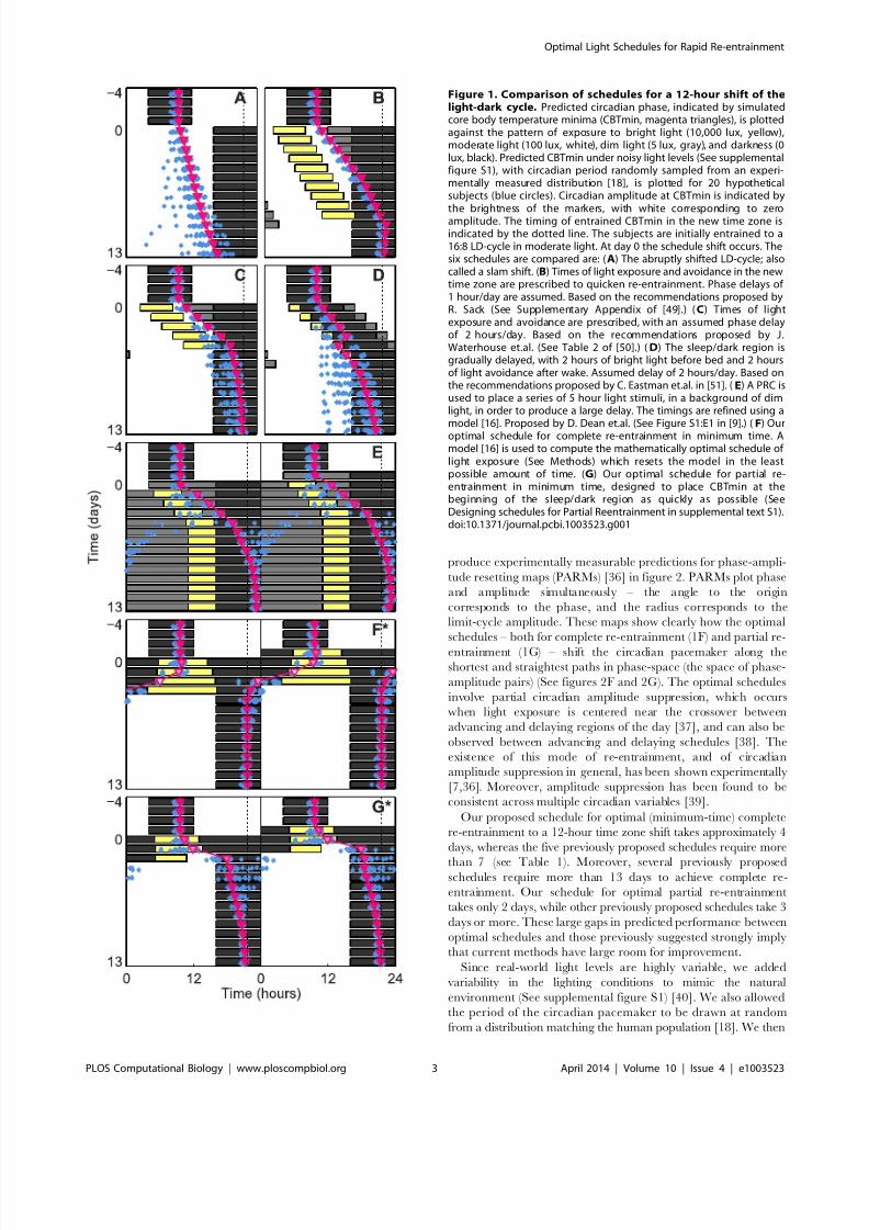
In figure 1, we compare our optimal schedules (1F and 1G) to

five other previously proposed schedules (1A–1E) for re-entrain-

ment to a 12-hour time-zone shift (1A). We present all seven

schedules as actograms, where each new line represents a

subsequent day. Black indicates darkness. Gray indicates dim

light (5 lux). White indicates low room light (100 lux). Yellow

indicates bright light (10,000 lux). In the original time zone, days

24 to 21 show a light-dark schedule of 16 hours of 100 lux light

and 8 hours of darkness (LD 16:8). At time 0 of day 0, we assume a

transition occurs. A magenta triangle shows the predicted timing

of the core body temperature minimum (CBTmin), a key circadianmarker that, when entrained, occurs slightly after the midpoint of

the dark episode. The brightness of the triangle’s face represents

the strength of the timekeeping signal, or the circadianamplitude, with white corresponding to zero amplitude. A blue

dot also shows the predicted timing of CBTmin, except under

conditions approximating real-world variations in light-levels and

inter-individual differences, the details of which are explained in

the sequel. The blue dots predict the CBTmin of twenty

hypothetical subjects, rather than one.

To study the effects of these schedules, we also plot the process

of re-entrainment in terms of both phase and amplitude. Thus, we

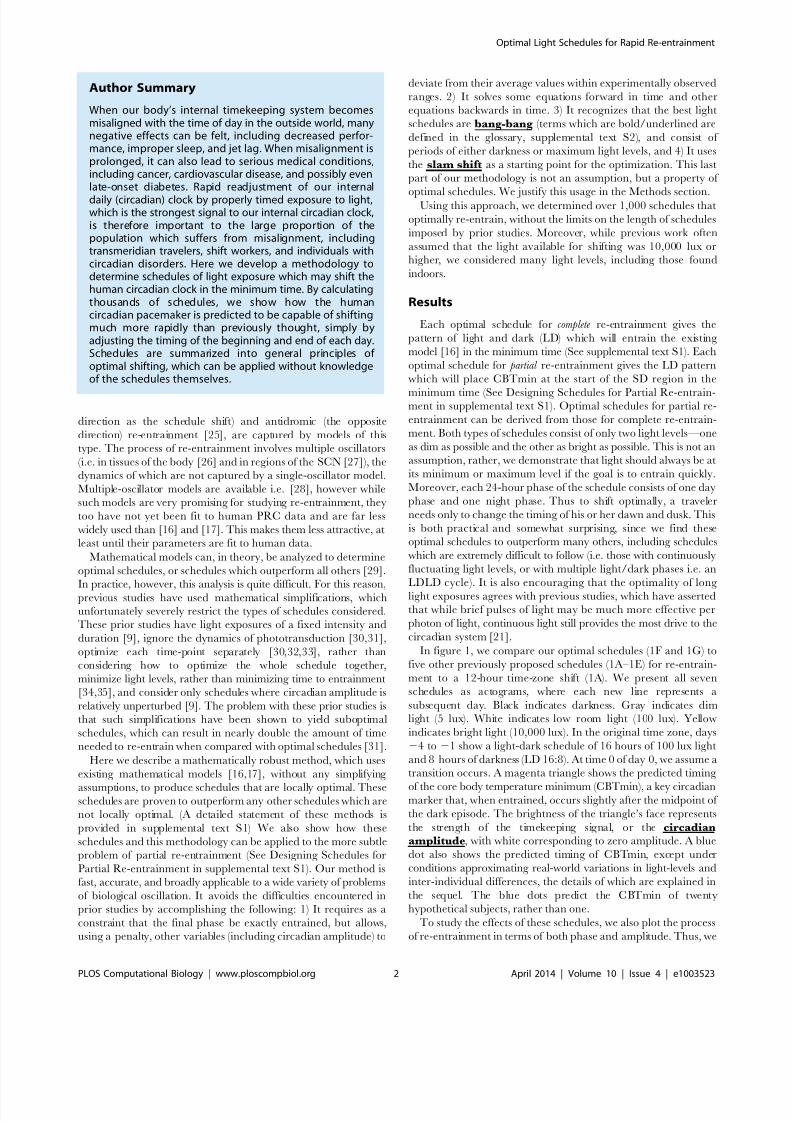
Author Summary

When our body’s internal timekeeping system becomesmisaligned with the time of day in the outside world, manynegative effects can be felt, including decreased perfor-mance, improper sleep, and jet lag. When misalignment isprolonged, it can also lead to serious medical conditions,including cancer, cardiovascular disease, and possibly evenlate-onset diabetes. Rapid readjustment of our internal

daily (circadian) clock by properly timed exposure to light,which is the strongest signal to our internal circadian clock,is therefore important to the large proportion of thepopulation which suffers from misalignment, includingtransmeridian travelers, shift workers, and individuals withcircadian disorders. Here we develop a methodology todetermine schedules of light exposure which may shift thehuman circadian clock in the minimum time. By calculatingthousands of schedules, we show how the humancircadian pacemaker is predicted to be capable of shiftingmuch more rapidly than previously thought, simply byadjusting the timing of the beginning and end of each day.Schedules are summarized into general principles of optimal shifting, which can be applied without knowledgeof the schedules themselves.

Optimal Light Schedules for Rapid Re-entrainment




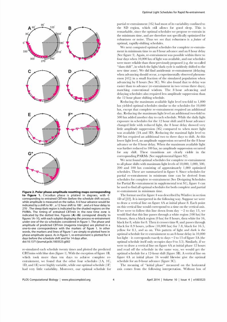
produce experimentally measurable predictions for phase-ampli-

tude resetting maps (PARMs) [36] in figure 2. PARMs plot phase

and amplitude simultaneously – the angle to the origin

corresponds to the phase, and the radius corresponds to the

limit-cycle amplitude. These maps show clearly how the optimal

schedules – both for complete re-entrainment (1F) and partial re-

entrainment (1G) – shift the circadian pacemaker along the

shortest and straightest paths in phase-space (the space of phase-

amplitude pairs) (See figures 2F and 2G). The optimal schedules

involve partial circadian amplitude suppression, which occurs

when light exposure is centered near the crossover between

advancing and delaying regions of the day [37], and can also be

observed between advancing and delaying schedules [38]. The

existence of this mode of re-entrainment, and of circadian

amplitude suppression in general, has been shown experimentally

[7,36]. Moreover, amplitude suppression has been found to be

consistent across multiple circadian variables [39].

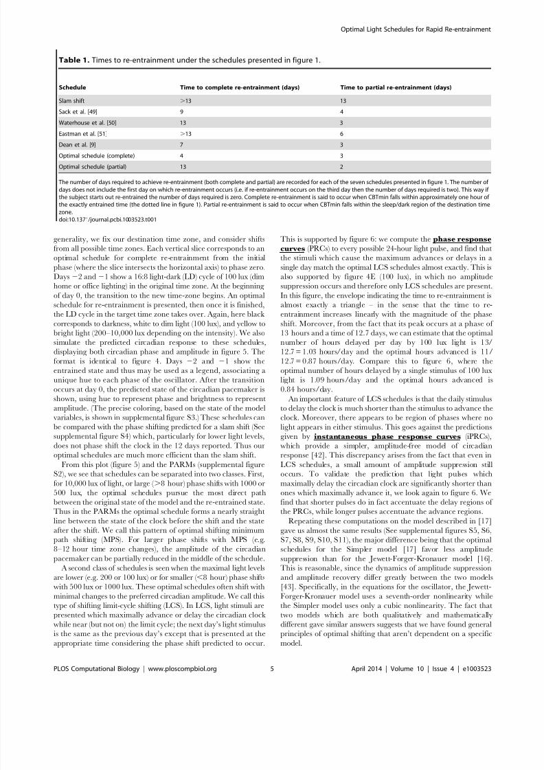
Our proposed schedule for optimal (minimum-time) complete

re-entrainment to a 12-hour time zone shift takes approximately 4

days, whereas the five previously proposed schedules require more

than 7 (see Table 1). Moreover, several previously proposedschedules require more than 13 days to achieve complete re-

entrainment. Our schedule for optimal partial re-entrainment

takes only 2 days, while other previously proposed schedules take 3

days or more. These large gaps in predicted performance between

optimal schedules and those previously suggested strongly imply

that current methods have large room for improvement.

Since real-world light levels are highly variable, we added

variability in the lighting conditions to mimic the natural

environment (See supplemental figure S1) [40]. We also allowed

the period of the circadian pacemaker to be drawn at random

from a distribution matching the human population [18]. We then

Figure 1. Comparison of schedules for a 12-hour shift of thelight-dark cycle. Predicted circadian phase, indicated by simulatedcore body temperature minima (CBTmin, magenta triangles), is plottedagainst the pattern of exposure to bright light (10,000 lux, yellow),moderate light (100 lux, white), dim light (5 lux, gray), and darkness (0lux, black). Predicted CBTmin under noisy light levels (See supplementalfigure S1), with circadian period randomly sampled from an experi-mentally measured distribution [18], is plotted for 20 hypotheticalsubjects (blue circles). Circadian amplitude at CBTmin is indicated bythe brightness of the markers, with white corresponding to zeroamplitude. The timing of entrained CBTmin in the new time zone isindicated by the dotted line. The subjects are initially entrained to a16:8 LD-cycle in moderate light. At day 0 the schedule shift occurs. Thesix schedules are compared are: (A) The abruptly shifted LD-cycle; alsocalled a slam shift. (B) Times of light exposure and avoidance in the newtime zone are prescribed to quicken re-entrainment. Phase delays of 1 hour/day are assumed. Based on the recommendations proposed byR. Sack (See Supplementary Appendix of [49].) (C) Times of lightexposure and avoidance are prescribed, with an assumed phase delayof 2 hours/day. Based on the recommendations proposed by J.Waterhouse et.al. (See Table 2 of [50].) (D) The sleep/dark region isgradually delayed, with 2 hours of bright light before bed and 2 hoursof light avoidance after wake. Assumed delay of 2 hours/day. Based onthe recommendations proposed by C. Eastman et.al. in [51]. (E) A PRC isused to place a series of 5 hour light stimuli, in a background of dimlight, in order to produce a large delay. The timings are refined using amodel [16]. Proposed by D. Dean et.al. (See Figure S1:E1 in [9].) (F) Ouroptimal schedule for complete re-entrainment in minimum time. Amodel [16] is used to compute the mathematically optimal schedule of light exposure (See Methods) which resets the model in the leastpossible amount of time. (G) Our optimal schedule for partial re-entrainment in minimum time, designed to place CBTmin at thebeginning of the sleep/dark region as quickly as possible (SeeDesigning schedules for Partial Reentrainment in supplemental text S1).doi:10.1371/journal.pcbi.1003523.g001





re-simulated each schedule twenty times and plotted the predicted

CBTmins with blue dots (figure 1). With the exception of figure 1B,

which took more than ten days to achieve complete re-

entrainment, we found that the other four schedules (1A, 1C,

1D, and 1E) were highly variable, while our optimal schedule (1F)

had very little variability. Moreover, our optimal schedule for

partial re-entrainment (1G) had most of its variability confined to

the SD region, which still allows for good sleep. This is

remarkable, since the optimal schedules we propose re-entrain in

the minimum time, and are therefore not specifically optimized for

robustness or noise. Thus we see that robustness is a feature of

optimal, rapidly-shifting schedules.

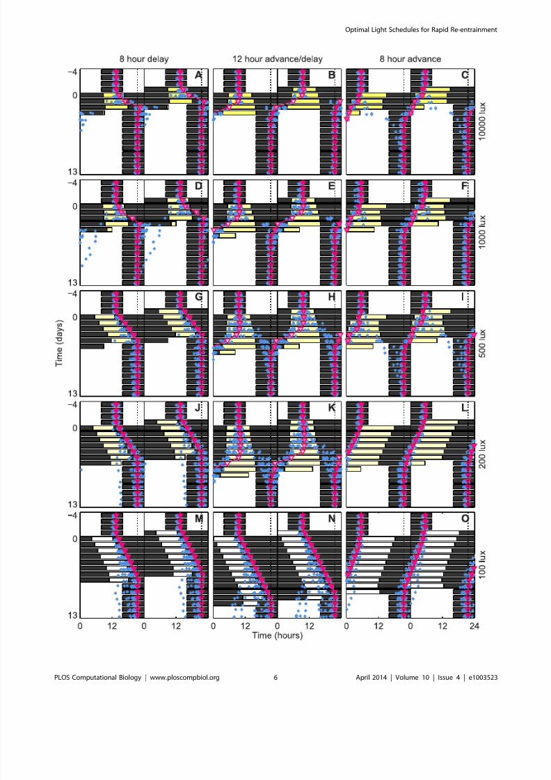
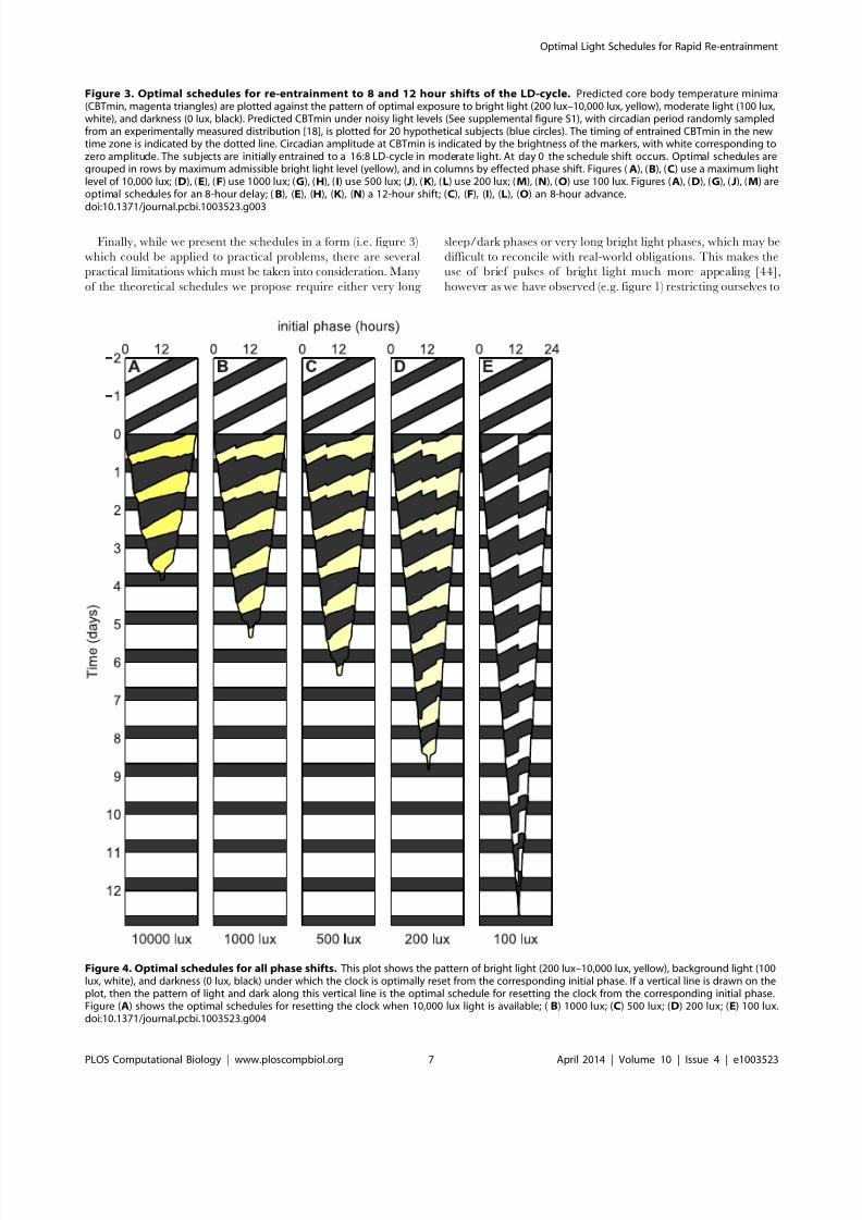
We next computed optimal schedules for complete re-entrain-

ment in minimum time to an 8 hour advance and an 8 hour delay

(See figure 3). Again, re-entrainment was possible within three tofour days when 10,000 lux of light was available, and our schedules

were more reliable than those previously proposed (e.g. the so-called

‘‘slam shift’’, in which the light/dark cycle is suddenly shifted to the

new time zone). We did find antidromic re-entrainment (delaying

when advancing should occur, a experimentally observed phenom-

enon [41]) in a small fraction of the simulated population when

advancing by 8 hours (See 3C). We also found that to delay was

easier than to advance (re-entrainment in two versus three days),

matching conventional wisdom. The 8 hour advancing and

delaying schedules also required less amplitude suppression than

the 12 hour phase shifting schedule.

Reducing the maximum available light level ten-fold to 1,000

lux yielded optimal schedules similar to the schedules for 10,000

lux, except that complete re-entrainment required an additional

day. Reducing the maximum light level an additional two-fold to500 lux added another day to each schedule. While the daily light

exposure in schedules for the 12 hour shift and 8 hour advance

changed little with reduced light, the 8 hour delay showed very

little amplitude suppression (3G) compared to when more light

was available (3A and 3D). Reducing the maximal light level to

200 lux required an additional two to three days to shift. At this

lower light level, no amplitude suppression occurred for the 8 hour

advance or the 8 hour delay. When the maximum available light

was further reduced to 100 lux, no amplitude suppression occurred

for any shift. These transitions are clearly visible in the

corresponding PARMs (See supplemental figure S2).

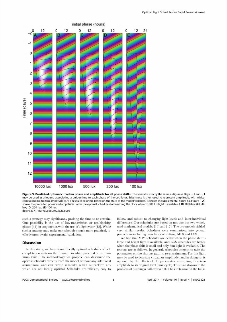
We next found optimal schedules for complete re-entrainment

to all phase shifts with maximum light levels of 10,000, 1,000, 500,

200 and 100 lux consisting of approximately 1,000 optimizedschedules. These are summarized in figure 4. Since schedules for

partial re-entrainment in minimum time can be derived from

schedules for complete re-entrainment (See Designing Schedules

for Partial Re-entrainment in supplemental text S1), figure 4 can

be used to find all optimal schedules for both complete and partial

re-entrainment in minimum time.

The format used in figure 4 was described by Winfree in section

1D of [22]. It is interpreted in the following way. Suppose we were

to draw a vertical line on figure 4A at initial phase 8. Each point

on this vertical line would correspond to a time on the vertical axis.

If we were to follow this line down from day 22 to day 13, we

would find that this line passes through a white region (100 lux) for

8 hours, then a black region (0 lux) for 8 hours, then white for 16,

black for 8, white for 8. Then it crosses time 0, and passes through

black for 8.9 hours, yellow (10,000 lux) for 7.8, black for 16.5, yellow for 8.1, and so on. This pattern of light and dark is the

optimal schedule for re-entrainment to an 8-hour delay in 10,000

lux light – it corresponds exactly to days 22 to 13 of figure 3A (the

optimal schedule itself only occupies days 0 to 3.5). Similarly, if we

were to draw a vertical line on figure 4A at initial phase 12 hours

and read off the schedule in the same way, we would get the

optimal schedule for a 12-hour shift (figure 3B). A vertical line on

figure 4A at initial phase 16 would likewise give the optimal

schedule for an 8-hour advance (figure 3C).

The meaning of ‘‘initial phase’’ measured on the horizontal

axis comes from the following interpretation. Without loss of

Figure 2. Polar phase-amplitude resetting maps correspondingto figure 1. Circadian phase is plotted in degrees, with 0ucorresponding to entrained CBTmin (before the schedule shift occurs),while amplitude is measured on the radius. A 6 hour advance would beindicated by a shift to 90u, a 12 hour shift to 180u, and a 6 hour delay to270u. The sleep/dark region is indicated by the shaded regions on thePARMs. The timing of entrained CBTmin in the new time zone isindicated by the dotted line. Figures (A)–(G) correspond directly tofigures 1A–1G, with each subplot displaying the process re-entrainmentunder one of the six schedules considered in figure 1. The phase and

amplitude of predicted CBTmin (magenta triangles) are plotted in aone-to-one correspondence with the markers of figure 1. In otherwords, the markers and lines of figure 1 are simply re-plotted here inphase-amplitude space. As in figure 1, re-entrainment is plotted for 4days before the schedule shift and for 14 days after.doi:10.1371/journal.pcbi.1003523.g002





generality, we fix our destination time zone, and consider shifts

from all possible time zones. Each vertical slice corresponds to an

optimal schedule for complete re-entrainment from the initial

phase (where the slice intersects the horizontal axis) to phase zero.Days 22 and 21 show a 16:8 light-dark (LD) cycle of 100 lux (dim

home or office lighting) in the original time zone. At the beginning

of day 0, the transition to the new time-zone begins. An optimal

schedule for re-entrainment is presented, then once it is finished,

the LD cycle in the target time zone takes over. Again, here black

corresponds to darkness, white to dim light (100 lux), and yellow to

bright light (200–10,000 lux depending on the intensity). We also

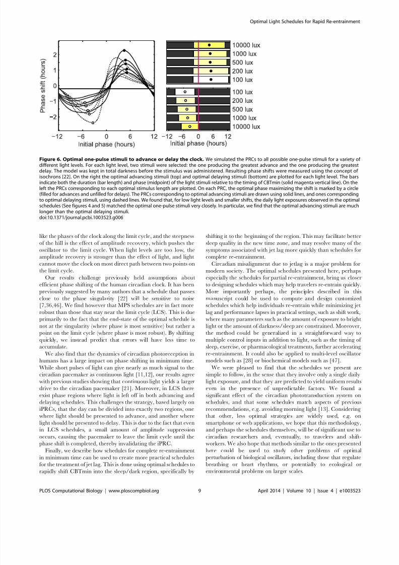
simulate the predicted circadian response to these schedules,

displaying both circadian phase and amplitude in figure 5. The

format is identical to figure 4. Days 22 and 21 show the

entrained state and thus may be used as a legend, associating a

unique hue to each phase of the oscillator. After the transition

occurs at day 0, the predicted state of the circadian pacemaker is

shown, using hue to represent phase and brightness to represent

amplitude. (The precise coloring, based on the state of the model

variables, is shown in supplemental figure S3.) These schedules can

be compared with the phase shifting predicted for a slam shift (See

supplemental figure S4) which, particularly for lower light levels,

does not phase shift the clock in the 12 days reported. Thus our

optimal schedules are much more efficient than the slam shift.

From this plot (figure 5) and the PARMs (supplemental figure

S2), we see that schedules can be separated into two classes. First,

for 10,000 lux of light, or large ( .8 hour) phase shifts with 1000 or

500 lux, the optimal schedules pursue the most direct path

between the original state of the model and the re-entrained state.

Thus in the PARMs the optimal schedule forms a nearly straight

line between the state of the clock before the shift and the state

after the shift. We call this pattern of optimal shifting minimum

path shifting (MPS). For larger phase shifts with MPS (e.g.8–12 hour time zone changes), the amplitude of the circadian

pacemaker can be partially reduced in the middle of the schedule.

A second class of schedules is seen when the maximal light levels

are lower (e.g. 200 or 100 lux) or for smaller ( ,8 hour) phase shifts

with 500 lux or 1000 lux. These optimal schedules often shift with

minimal changes to the preferred circadian amplitude. We call this

type of shifting limit-cycle shifting (LCS). In LCS, light stimuli are

presented which maximally advance or delay the circadian clock

while near (but not on) the limit cycle; the next day’s light stimulus

is the same as the previous day’s except that is presented at the

appropriate time considering the phase shift predicted to occur.

This is supported by figure 6: we compute the phase response

curves (PRCs) to every possible 24-hour light pulse, and find that

the stimuli which cause the maximum advances or delays in a

single day match the optimal LCS schedules almost exactly. This isalso supported by figure 4E (100 lux), in which no amplitude

suppression occurs and therefore only LCS schedules are present.

In this figure, the envelope indicating the time to re-entrainment is

almost exactly a triangle – in the sense that the time to re-

entrainment increases linearly with the magnitude of the phase

shift. Moreover, from the fact that its peak occurs at a phase of

13 hours and a time of 12.7 days, we can estimate that the optimal

number of hours delayed per day by 100 lux light is 13/

12.7 = 1.03 hours/day and the optimal hours advanced is 11/

12.7 = 0.87 hours/day. Compare this to figure 6, where the

optimal number of hours delayed by a single stimulus of 100 lux

light is 1.09 hours/day and the optimal hours advanced is

0.84 hours/day.

An important feature of LCS schedules is that the daily stimulus

to delay the clock is much shorter than the stimulus to advance the

clock. Moreover, there appears to be region of phases where no

light appears in either stimulus. This goes against the predictions

given by instantaneous phase response curves (iPRCs),

which provide a simpler, amplitude-free model of circadian

response [42]. This discrepancy arises from the fact that even in

LCS schedules, a small amount of amplitude suppression still

occurs. To validate the prediction that light pulses which

maximally delay the circadian clock are significantly shorter than

ones which maximally advance it, we look again to figure 6. We

find that shorter pulses do in fact accentuate the delay regions of

the PRCs, while longer pulses accentuate the advance regions.

Repeating these computations on the model described in [17]

gave us almost the same results (See supplemental figures S5, S6,

S7, S8, S9, S10, S11), the major difference being that the optimalschedules for the Simpler model [17] favor less amplitude

suppression than for the Jewett-Forger-Kronauer model [16].

This is reasonable, since the dynamics of amplitude suppression

and amplitude recovery differ greatly between the two models

[43]. Specifically, in the equations for the oscillator, the Jewett-

Forger-Kronauer model uses a seventh-order nonlinearity while

the Simpler model uses only a cubic nonlinearity. The fact that

two models which are both qualitatively and mathematically

different gave similar answers suggests that we have found general

principles of optimal shifting that aren’t dependent on a specific

model.

Table 1. Times to re-entrainment under the schedules presented in figure 1.

Schedule Time to complete re-entrainment (days) Time to partial re-entrainment (days)

Slam shift .13 13

Sack et al. [49] 9 4

Waterhouse et al. [50] 13 3

Eastman et al. [51] .13 6Dean et al. [9] 7 3

Optimal schedule (complete) 4 3

Optimal schedule (partial) 13 2

The number of days required to achieve re-entrainment (both complete and partial) are recorded for each of the seven schedules presented in figure 1. The number of days does not include the first day on which re-entrainment occurs (i.e. if re-entrainment occurs on the third day then the number of days required is two). This way if the subject starts out re-entrained the number of days required is zero. Complete re-entrainment is said to occur when CBTmin falls within approximately one hour of the exactly entrained time (the dotted line in figure 1). Partial re-entrainment is said to occur when CBTmin falls within the sleep/dark region of the destination timezone.doi:10.1371/journal.pcbi.1003523.t001









Finally, while we present the schedules in a form (i.e. figure 3)

which could be applied to practical problems, there are several

practical limitations which must be taken into consideration. Many

of the theoretical schedules we propose require either very long

sleep/dark phases or very long bright light phases, which may be

difficult to reconcile with real-world obligations. This makes the

use of brief pulses of bright light much more appealing [44],

however as we have observed (e.g. figure 1) restricting ourselves to

Figure 3. Optimal schedules for re-entrainment to 8 and 12 hour shifts of the LD-cycle. Predicted core body temperature minima(CBTmin, magenta triangles) are plotted against the pattern of optimal exposure to bright light (200 lux–10,000 lux, yellow), moderate light (100 lux,white), and darkness (0 lux, black). Predicted CBTmin under noisy light levels (See supplemental figure S1), with circadian period randomly sampledfrom an experimentally measured distribution [18], is plotted for 20 hypothetical subjects (blue circles). The timing of entrained CBTmin in the newtime zone is indicated by the dotted line. Circadian amplitude at CBTmin is indicated by the brightness of the markers, with white corresponding tozero amplitude. The subjects are initially entrained to a 16:8 LD-cycle in moderate light. At day 0 the schedule shift occurs. Optimal schedules aregrouped in rows by maximum admissible bright light level (yellow), and in columns by effected phase shift. Figures (A), (B), (C) use a maximum lightlevel of 10,000 lux; (D), (E), (F) use 1000 lux; (G), (H), (I) use 500 lux; (J), (K), (L) use 200 lux; (M), (N), (O) use 100 lux. Figures (A), (D), (G), (J), (M) areoptimal schedules for an 8-hour delay; (B), (E), (H), (K), (N) a 12-hour shift; (C), (F), (I), (L), (O) an 8-hour advance.doi:10.1371/journal.pcbi.1003523.g003

Figure 4. Optimal schedules for all phase shifts. This plot shows the pattern of bright light (200 lux–10,000 lux, yellow), background light (100lux, white), and darkness (0 lux, black) under which the clock is optimally reset from the corresponding initial phase. If a vertical line is drawn on theplot, then the pattern of light and dark along this vertical line is the optimal schedule for resetting the clock from the corresponding initial phase.Figure (A) shows the optimal schedules for resetting the clock when 10,000 lux light is available; ( B) 1000 lux; (C) 500 lux; (D) 200 lux; (E) 100 lux.doi:10.1371/journal.pcbi.1003523.g004





such a strategy may significantly prolong the time to re-entrain.

One possibility is the use of low-transmission or red-blocking

glasses [44] in conjunction with the use of a light visor [45]. Whilesuch a strategy may make our schedules much more practical, its

effectiveness awaits experimental validation.

Discussion

In this study, we have found locally optimal schedules which

completely re-entrain the human circadian pacemaker in mini-

mum time. The methodology we propose can determine the

optimal schedules directly from the model, without any additional

assumptions, and can create schedules which outperform any

which are not locally optimal. Schedules are efficient, easy to

follow, and robust to changing light levels and inter-individual

differences. Our schedules are based on not one but two widely

used mathematical models: [16] and [17]. The two models yielded very similar results. Schedules were summarized into general

predictions including two classes of shifting, MPS and LCS.

We find that MPS schedules are better when the phase shift is

large and bright light is available, and LCS schedules are better

when the phase shift is small and only dim light is available. The

reasons are as follows. In general, schedules attempt to take the

pacemaker on the shortest path to re-entrainment. For this light

may be used to decrease circadian amplitude, and in doing so, is

opposed by the effects of the pacemaker attempting to return

amplitude to its original level (limit cycle). This is analogous to the

problem of pushing a ball over a hill. The circle around the hill is

Figure 5. Predicted optimal circadian phase and amplitude for all phase shifts. The format is exactly the same as figure 4. Days 22 and 21may be used as a legend associating a unique hue to each phase of the oscillator. Brightness is then used to represent amplitude, with whitecorresponding to zero amplitude [37]. The exact coloring, based on the state of the model variables, is shown in supplemental figure S3. Figure ( A)shows the predicted phase and amplitude under the optimal schedules for resetting the clock when 10,000 lux light is available; ( B) 1000 lux; (C) 500lux; (D) 200 lux; (E) 100 lux.doi:10.1371/journal.pcbi.1003523.g005





like the phases of the clock along the limit cycle, and the steepness

of the hill is the effect of amplitude recovery, which pushes the

oscillator to the limit cycle. When light levels are too low, the

amplitude recovery is stronger than the effect of light, and light

cannot move the clock on most direct path between two points on

the limit cycle.

Our results challenge previously held assumptions about

efficient phase shifting of the human circadian clock. It has been

previously suggested by many authors that a schedule that passes

close to the phase singularity [22] will be sensitive to noise[7,36,46]. We find however that MPS schedules are in fact more

robust than those that stay near the limit cycle (LCS). This is due

primarily to the fact that the end-state of the optimal schedule is

not at the singularity (where phase is most sensitive) but rather a

point on the limit cycle (where phase is most robust). By shifting

quickly, we instead predict that errors will have less time to

accumulate.

We also find that the dynamics of circadian photoreception in

humans has a large impact on phase shifting in minimum time.

While short pulses of light can give nearly as much signal to the

circadian pacemaker as continuous light [11,12], our results agree

with previous studies showing that continuous light yields a larger

drive to the circadian pacemaker [21]. Moreover, in LCS there

exist phase regions where light is left off in both advancing anddelaying schedules. This challenges the strategy, based largely on

iPRCs, that the day can be divided into exactly two regions, one

where light should be presented to advance, and another where

light should be presented to delay. This is due to the fact that even

in LCS schedules, a small amount of amplitude suppression

occurs, causing the pacemaker to leave the limit cycle until the

phase shift is completed, thereby invalidating the iPRC.

Finally, we describe how schedules for complete re-entrainment

in minimum time can be used to create more practical schedules

for the treatment of jet lag. This is done using optimal schedules to

rapidly shift CBTmin into the sleep/dark region, specifically by

shifting it to the beginning of the region. This may facilitate better

sleep quality in the new time zone, and may resolve many of the

symptoms associated with jet lag more quickly than schedules for

complete re-entrainment.

Circadian misalignment due to jetlag is a major problem for

modern society. The optimal schedules presented here, perhaps

especially the schedules for partial re-entrainment, bring us closer

to designing schedules which may help travelers re-entrain quickly.

More importantly perhaps, the principles described in this

manuscript could be used to compute and design customizedschedules which help individuals re-entrain while minimizing jet

lag and performance lapses in practical settings, such as shift work,

where many parameters such as the amount of exposure to bright

light or the amount of darkness/sleep are constrained. Moreover,

the method could be generalized in a straightforward way to

multiple control inputs in addition to light, such as the timing of

sleep, exercise, or pharmacological treatments, further accelerating

re-entrainment. It could also be applied to multi-level oscillator

models such as [28] or biochemical models such as [47].

We were pleased to find that the schedules we present are

simple to follow, in the sense that they involve only a single daily

light exposure, and that they are predicted to yield uniform results

even in the presence of unpredictable factors. We found a

significant effect of the circadian phototransduction system onschedules, and that some schedules match aspects of previous

recommendations, e.g. avoiding morning light [13]. Considering

that other, less optimal strategies are widely used, e.g. on

smartphone or web applications, we hope that this methodology,

and perhaps the schedules themselves, will be of significant use to

circadian researchers and, eventually, to travelers and shift-

workers. We also hope that methods similar to the ones presented

here could be used to study other problems of optimal

perturbation of biological oscillators, including those that regulate

breathing or heart rhythms, or potentially to ecological or

environmental problems on larger scales.

Figure 6. Optimal one-pulse stimuli to advance or delay the clock. We simulated the PRCs to all possible one-pulse stimuli for a variety of different light levels. For each light level, two stimuli were selected: the one producing the greatest advance and the one producing the greatestdelay. The model was kept in total darkness before the stimulus was administered. Resulting phase shifts were measured using the concept of isochrons [22]. On the right the optimal advancing stimuli (top) and optimal delaying stimuli (bottom) are plotted for each light level. The barsindicate both the duration (bar length) and phase (midpoint) of the light stimuli relative to the timing of CBTmin (solid magenta vertical line). On theleft the PRCs corresponding to each optimal stimulus length are plotted. On each PRC, the optimal phase maximizing the shift is marked by a circle(filled for advances and unfilled for delays). The PRCs corresponding to optimal advancing stimuli are drawn using solid lines, and ones correspondingto optimal delaying stimuli, using dashed lines. We found that, for low light levels and smaller shifts, the daily light exposures observed in the optimalschedules (See figures 4 and 5) matched the optimal one-pulse stimuli very closely. In particular, we find that the optimal advancing stimuli are muchlonger than the optimal delaying stimuli.doi:10.1371/journal.pcbi.1003523.g006





Methods

Our methodology to compute optimal schedules consists of twomajor contributions. First, we define the re-entrainment problem

in terms of optimal control theory. This includes computing the

isochrons of the model. Second, we compute the optimal

solution using a novel numerical algorithm based on a method

originally used to optimize robotic manipulators. These steps are

covered in great detail in supplemental text S1 – we summarize

them briefly as follows.

The models we use [16,17] comprise a system of ordinary

differential equations. These equations should relate the state of

the model, which we call x~(x1,x2, . . . ,xn), to the time t and a

control (e.g. light) which we call u – we should be able to write

them in this form:

dx1

dt ~ f 1(x,u,t)

dx2

dt ~ f 2(x,u,t)

.

.

.

dxn

dt ~ f n(x,u,t)

We formulate an ‘‘optimal control’’ problem by defining two

functions of x and t: the ‘‘constraint’’ y(x,t) which must equal 0 at

the final time t f , and represents the conditions we would like our

solution to satisfy, and the ‘‘cost’’ Q(x,t), which represents the

quantity we would like to minimize at the final time t f .

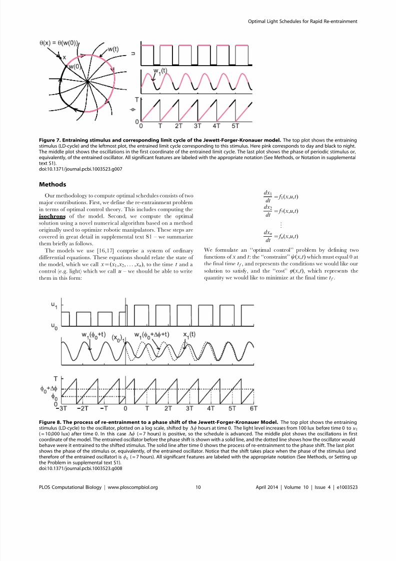
Figure 7. Entraining stimulus and corresponding limit cycle of the Jewett-Forger-Kronauer model. The top plot shows the entrainingstimulus (LD-cycle) and the leftmost plot, the entrained limit cycle corresponding to this stimulus. Here pink corresponds to day and black to night.The middle plot shows the oscillations in the first coordinate of the entrained limit cycle. The last plot shows the phase of periodic stimulus or,equivalently, of the entrained oscillator. All significant features are labeled with the appropriate notation (See Methods, or Notation in supplementaltext S1).doi:10.1371/journal.pcbi.1003523.g007

Figure 8. The process of re-entrainment to a phase shift of the Jewett-Forger-Kronauer Model. The top plot shows the entrainingstimulus (LD-cycle) to the oscillator, plotted on a log scale, shifted by Dw hours at time 0. The light level increases from 100 lux before time 0 to u1

( = 10,000 lux) after time 0. In this case Dw ( = 7 hours) is positive, so the schedule is advanced. The middle plot shows the oscillations in firstcoordinate of the model. The entrained oscillator before the phase shift is shown with a solid line, and the dotted line shows how the oscillator wouldbehave were it entrained to the shifted stimulus. The solid line after time 0 shows the process of re-entrainment to the phase shift. The last plotshows the phase of the stimulus or, equivalently, of the entrained oscillator. Notice that the shift takes place when the phase of the stimulus (andtherefore of the entrained oscillator) is w0 ( = 7 hours). All significant features are labeled with the appropriate notation (See Methods, or Setting upthe Problem in supplemental text S1).doi:10.1371/journal.pcbi.1003523.g008





The constraint is defined as follows. Unlike previous works, we

explicitly compute the isochrons of the model in the form of a

function h(x), which gives the model’s phase for any state x . We

also compute the entrained (or forced) limit-cycle w(w), which

gives the state of the entrained model as a function of the phase w,

which is defined as the remainder of time t divided by 24 hours

(see figure 7). We use w(w) and w(t) interchangeably where the

meaning is clear. Beginning our optimization at phase w0 and state

x0~

w(w0), to achieve a phase shift of D

w hours we require that att f the final phase is equal to the re-entrained phase, or that

h(x(t f ))~h(w(w0zDwzt f )) (See figure 8). Therefore, we set

y(x,t)~h(x){h(w(w0zDwzt)). This guarantees that the final

phase is exactly entrained, which has heretofore not been done.

The cost is defined in the following way. Since we would like to

minimize time t, a natural cost function would be Q(x,t)~t.

However, we would also like to control how much circadian

amplitude is recovered, as more amplitude recovery is desirable. If

we compute amplitude with the function A(x), then this can be

accomplished with the penalty ½A(x){A(w(w0zDwzt))2, which

we add to the cost with the coefficient C : Q(x,t)~

tzC ½A(x){A(w(w0zDwzt))2. This novel approach allows us

to control how much amplitude is recovered by adjusting the size

of C .

Once we have an optimal control problem to solve, we compute

its solution using a numerical algorithm. We use a novel

modification of a numerical method called the Switch Time

Optimization method [48]. This method assumes that the control

is ‘‘bang-bang,’’ meaning that it switches between the minimum

and maximum levels. In fact, we show that such a control is

optimal (See supplemental text S1). The algorithm works

by computing so-called ‘‘sensitivity functions’’ lT y (t)~

dy(x(t f ),t f )=dx(t) and lT J (t)~dQ(x(t f ),t f )=dx(t), which relate

changes in the state of the model at time t to the final constraint

and final cost respectively. At each step, the algorithm takes the

previous set of switching times, and using these sensitivity functions

computes a set of small changes which, when added to these

switching times, will decrease the cost function while keeping the

constraint satisfied. The critical modification allowing thisalgorithm to work on the problem of minimum time re-

entrainment is step 4 of the method, which precisely controls thestep size. This novel contribution to the method significantly

improves its rate of convergence – without it the original algorithm

in [48] fails. The final algorithm is given below:

Step 1 Guess nominal terminal time t f and switching times t1,t2, . . . ,tq on½0,t f .

Step 2 Determine the trajectory x(t) by integrating the system equations forward from x0 using these switching times.

Step 3 Determine the sensitivity functions lJ (t) and ly(t) by integrating backwards

_llT J ~{lT

J L f Lx

(x(t),u(t),t) with lT J (t f )~ LQ

Lx

t f

,

and

_llT

y~{lT y

L f

Lx(x(t),u(t),t) with lT

y (t f )~Ly

Lx

t f

:

Step 4 Let Du j be the jump in the control at time t j , with positive sign for a

jump ‘‘down’’ and negative for a jump ‘‘up.’’ Choose some small Et f w0 and,

denoting the fastest timescale of the problem by tsw0, set

Eu~ts=max j

1

Du j

lT J

L f

Lu

t j

:

Step 5 Determine the optimal perturbations for decreasing Q(x(t f ),t f )

dtJ j ~{

Eu

Du j

lT J

L f Lu

t j

and dtJ f ~{Et f

LQLtzlT

J f

t f

,

and for increasing y(x(t f ),t f )

dty

j ~Eu

Du j

lT y

L f

Lu

t j

and dty

f ~Et f

Ly

LtzlT

y f

t f

:

Step 6 Determine the effect of these perturbations on y(x(t f ),t f )

d yJ ~

Ly

LtzlT

y f

t f

dtJ f zX

q

j ~1

lT y

L f

Lu

t j

Du j dtJ j ,

and

d yy~

Ly

LtzlT

y f

t f

dty

f z

Xq

j ~1

lT y

L f

Lu

t j

Du j dty

j :

Step 7 Choose some small Eyw0 and set

n~{Eyy(x(t f ),t f ){d yJ

d yy :

Step 8 Record the optimal increments dtJ J

j ~dtJ j zndt

y j for j ~1, . . . ,q

and dtJ J

f ~dtJ f zndt

y f . Then update the solution with t j /t j zdt

J J j for

j ~1, . . . ,q and t f /t f zdtJ J

f .

When this algorithm converges – in the sense that the guess can

no longer be improved – we find that the solution satisfies a set of

local optimality conditions called Pontryagin’s Minimum Principle

(see supplemental text S1). Hence this algorithm takes any initial

guess for the control and improves it until it is locally optimal.

Supporting Information

Figure S1 Example of noisy light levels. ( A ) shows the light

schedule for re-entraining to a 12-hour shift in minimum time (Seefigure 1F). ( B ) shows this same light schedule, but with noise

imitating experimentally observed variations in light intensity [40].

The random noise was produced as follows. Every 10 minutes a

number was sampled from a standard normal distribution. These

numbers were then linearly interpolated to get a function of time.

The schedule was then transformed to a log scale and the noise

was added. The result is normally distributed noise added on a log

scale, with a standard deviation of one order of magnitude.

(EPS)

Figure S2 Polar phase-amplitude resetting maps corre-sponding to figure 3. Circadian phase is plotted in degrees,





with 0u corresponding to entrained CBTmin (before the schedule

shift occurs), while amplitude is measured on the radius. A 6 hour

advance would be indicated by a shift to 90u, a 12 hour shift to

180u, and a 6 hour delay to 270u. The sleep/dark region is

indicated by the shaded regions on the PARMs. The timing of

entrained CBTmin in the new time zone is indicated by the dotted

line. Figures ( A )–( O ) correspond directly to figures 3A–3O, with

each subplot displaying the process re-entrainment under one of

the 15 schedules considered in figure 3. The phase and amplitudeof predicted CBTmin (magenta triangles) are plotted in a one-to-

one correspondence with the markers of figure 3. In other words,

the markers and lines of figure 3 are simply re-plotted here in

phase-amplitude space. As in figure 3, re-entrainment is plotted for

4 days before the schedule shift and for 14 days after.

(EPS)

Figure S3 Isochrons and limit cycle of the Jewett-Forger-Kronauer Model. The limit cycle and isochrons (curves

of constant phase) of the model [16] are plotted in 2-dimensional

phase space [22]. The horizontal axis corresponds to the variable

x in the model; the vertical to xc. The color indicates phase by its

hue and amplitude by its brightness, with white representing zero

amplitude [37]. Isochrons were computed using backwards

integration [42]. The white regions at ( 21,1) and (1,21) couldnot be computed because trajectories diverged too rapidly.

(TIF)

Figure S4 Predicted circadian phase and amplitudeunder the slam shift. Days 22 and 21 correspond to a 16:8

LD-cycle of 100 lux. At day 0 the schedule shift occurs. The

brightness of light in the shifted LD-cycle (time .0) varies from

100 lux to 10,000 lux according to the labels on the subplots.

Predictions were made using the Jewett-Forger-Kronauer model

[16]. Days 22 and 21 may be used as a legend associating a

unique hue to each phase of the oscillator. Brightness is then used

to represent amplitude, with white corresponding to zero

amplitude [37]. The exact coloring, based on the state of the

model variables, is shown in supplemental figure S3. Figure ( A )

shows the predicted phase and amplitude under the slam shift with10,000 lux light in the new time zone; ( B ) 1000 lux; ( C ) 500 lux;

( D ) 200 lux; ( E ) 100 lux.

(TIF)

Figure S5 Optimal schedules for re-entrainment to 8and 12 hour shifts of the LD-cycle (Simpler model).

Predicted core body temperature minima (CBTmin, magenta

triangles) are plotted against the pattern of optimal exposure to

bright light (200 lux–10,000 lux, yellow), moderate light (100 lux,

white), and darkness (0 lux, black). Predicted CBTmin under noisy

light levels (See supplemental figure S1), with circadian period

randomly sampled from an experimentally measured distribution

[18], is plotted for 20 hypothetical subjects (blue circles). The

timing of entrained CBTmin in the new time zone is indicated by

the dotted line. Circadian amplitude at CBTmin is indicated bythe brightness of the markers, with white corresponding to zero

amplitude. The subjects are initially entrained to a 16:8 LD-cycle

in moderate light. At day 0 the schedule shift occurs. Optimal

schedules are grouped in rows by maximum admissible bright light

level (yellow), and in columns by effected phase shift. Figures ( A ),( B ), ( C ) use a maximum light level of 10,000 lux; ( D ), ( E ), ( F ) use

1000 lux; ( G ), ( H ), ( I ) use 500 lux; ( J ), ( K ), ( L ) use 200 lux; ( M ), ( N ),

( O ) use 100 lux. Figures ( A ), ( D ), ( G ), ( J ), ( M ) are optimal schedules

for an 8-hour delay; ( B ), ( E ), ( H ), ( K ), ( N ) a 12-hour shift; ( C ), ( F ),

( I ), ( L ), ( O ) an 8-hour advance.

(EPS)

Figure S6 Polar phase-amplitude resetting maps corre-sponding to supplemental figure S5 (Simpler model).Circadian phase is plotted in degrees, with 0u corresponding to

entrained CBTmin (before the schedule shift occurs), while

amplitude is measured on the radius. A 6 hour advance would

be indicated by a shift to 90u, a 12 hour shift to 180u, and a 6 hour

delay to 270u. The sleep/dark region is indicated by the shaded

regions on the PARMs. The timing of entrained CBTmin in the

new time zone is indicated by the dotted line. Figures ( A )–( O )correspond directly to figures S5A–S5O, with each subplot

displaying the process re-entrainment under one of the 15

schedules considered in figure S5. The phase and amplitude of

predicted CBTmin (magenta triangles) are plotted in a one-to-

one correspondence with the markers of figure S5. In other

words, the markers and lines of figure S5 are simply re-plotted

here in phase-amplitude space. As in figure S5, re-entrainment

is plotted for 4 days before the schedule shift and for 14 days

after.

(EPS)

Figure S7 Optimal schedules for all phase shifts(Simpler model). This plot shows the pattern of bright light

(200 lux–10,000 lux, yellow), background light (100 lux, white),

and darkness (0 lux, black) under which the clock is optimally resetfrom the corresponding initial phase. If a vertical line is drawn on

the plot, then the pattern of light and dark along this vertical line is

the optimal schedule for resetting the clock from the correspond-

ing initial phase. Figure ( A ) shows the optimal schedules for

resetting the clock when 10,000 lux light is available; ( B ) 1000 lux;

( C ) 500 lux; ( D ) 200 lux; ( E ) 100 lux.

(EPS)

Figure S8 Predicted optimal circadian phase andamplitude for all phase shifts (Simpler model). The

format is exactly the same as figure S7. Days 22 and 21 may be

used as a legend associating a unique hue to each phase of the

oscillator. Brightness is then used to represent amplitude, with

white corresponding to zero amplitude [37]. The exact coloring,

based on the state of the model variables, is shown in supplementalfigure S9. Figure ( A ) shows the predicted phase and amplitude

under the optimal schedules for resetting the clock when 10,000

lux light is available; ( B ) 1000 lux; ( C ) 500 lux; ( D ) 200 lux; ( E ) 100

lux.

(TIF)

Figure S9 Isochrons and limit cycle of the Simplermodel. The limit cycle and isochrons (curves of constant phase) of

the model [17] are plotted in 2-dimensional phase space [22]. The

horizontal axis corresponds to the variable x in the model; the

vertical to xc. The color indicates phase by its hue and amplitude

by its brightness, with white representing zero amplitude [37].

Isochrons were computed using backwards integration [42]. The

white regions at ( 21,21) and (1,1) could not be computed because

trajectories diverged too rapidly.(TIF)

Figure S10 Predicted circadian phase and amplitudeunder the slam shift (Simpler model). Days 22 and 21

correspond to a 16:8 LD-cycle of 100 lux. At day 0 the schedule

shift occurs. The brightness of light in the shifted LD-cycle (time

.0) varies from 100 lux to 10,000 lux according to the labels on

the subplots. Predictions were made using the Simpler model [17].

Days 22 and 21 may be used as a legend associating a unique

hue to each phase of the oscillator. Brightness is then used to

represent amplitude, with white corresponding to zero amplitude

[37]. The exact coloring, based on the state of the model variables,





is shown in supplemental figure S9. This format for displaying the

process of re-entrainment is used in section of 1D of [22].(TIF)

Figure S11 Optimal one-pulse stimuli to advance ordelay the clock (Simpler model). We simulated the PRCs to

all possible one-pulse stimuli for a variety of different light levels.

For each light level, two stimuli were selected: the one producing

the greatest advance and the one producing the greatest delay.

The model was kept in total darkness before the stimulus wasadministered. Resulting phase shifts were measured using the

concept of isochrons [22]. On the right the optimal advancing

stimuli (top) and optimal delaying stimuli (bottom) are plotted for

each light level. The bars indicate both the duration (bar length)

and phase (midpoint) of the light stimuli relative to the timing of

CBTmin (solid magenta vertical line). On the left the PRCscorresponding to each optimal stimulus length are plotted. On

each PRC, the optimal phase maximizing the shift is marked by a

circle (filled for advances and unfilled for delays). The PRCs

corresponding to optimal advancing stimuli are drawn using solid

lines, and ones corresponding to optimal delaying stimuli, using

dashed lines. We found that, for low light levels and smaller shifts,

the daily light exposures observed in the optimal schedules (See

figures S7 and S8) matched the optimal one-pulse stimuli very

closely. In particular, we find that the optimal advancing stimuli

are much longer than the optimal delaying stimuli.

(EPS)

Figure S12 Optimal trajectories corresponding tofigure 3. The optimal trajectories are plotted in phase space.

The horizontal axis corresponds to the variable x in the model; the

vertical to xc. The limit cycle is shown by the dotted line and the

trajectory of the model is shown by the solid line. The isochron

representing entrained circadian phase at the terminal time is

shown by the thick solid line. The times when the light switches on

are marked by the bright purple circles; times when it switches off

are marked by the dark purple xs (the control is bang-bang). The

time when the optimal schedule begins is marked by a small black

circle on the limit cycle. The figures ( A )–( O ) correspond directly

to figures 3A–3O, with each subplot displaying the processre-entrainment under one of the 15 schedules considered in

figure 3.

(EPS)

Figure S13 Optimal controls and Hamiltonians corre-sponding to figure 3. The optimal control I (equivalently a for

the purposes of schedule design) is plotted in black against the

quantity LH =Lu, shown by a red curve. For the control to be

optimal it is necessary that at each time t, the control u (i.e. a )minimizes H (x(t),u,t) (See condition (2) in PMP2 in supplemental

text S1). Since u appears linearly in H , we see that LH =Lu gives

the coefficient of u in H (x(t),u,t). Thus when LH =Luw0 the

control must take its minimum value and when LH =Luv0 the

control must take its maximum value. This is precisely what we see

in all the plots on the right. Thus the condition is satisfied. The

figures ( A )–( O ) correspond directly to figures 3A–3O, with each

subplot displaying the optimal schedule and Hamiltonian

derivative for one of the 15 schedules.

(EPS)

Figure S14 Optimal trajectories corresponding to figure

S5 (Simpler model). The optimal trajectories are plotted in

phase space. The horizontal axis corresponds to the variable x in

the model; the vertical to xc. The limit cycle is shown by the dottedline and the trajectory of the model is shown by the solid line. The

isochron representing entrained circadian phase at the terminal

time is shown by the thick solid line. The times when the light

switches on are marked by the bright purple circles; times when it

switches off are marked by the dark purple xs (the control is bang-

bang). The time when the optimal schedule begins is marked by a

small black circle on the limit cycle. The figures ( A )–( O )

correspond directly to figures S5A–S5O, with each subplot

displaying the process re-entrainment under one of the 15

schedules considered in figure S5.

(EPS)

Figure S15 Optimal controls and Hamiltonians corre-sponding to supplemental figure S5 (Simpler model).

The optimal control I (equivalently a for the purposes of schedule

design) is plotted in black against the quantity LH =Lu, shown by a

red curve. For the control to be optimal it is necessary that at each

time t, the control u (i.e. a ) minimizes H (x(t),u,t) (See condition

(2) in PMP2 in supplemental text S1). Since u appears linearly in

H , we see that LH =Lu gives the coefficient of u in H (x(t),u,t).

Thus when LH =Luw0 the control must take its minimum value

and when LH =Luv0 the control must take its maximum value.

This is precisely what we see in all the plots on the right. Thus the

condition is satisfied. The figures ( A )–( O ) correspond directly to

figures S5A–S5O, with each subplot displaying the optimal

schedule and Hamiltonian derivative for one of the 15 schedules.

(EPS)

Text S1 Detailed methods. A detailed description of the

methods is provided.

(DOC)

Text S2 Glossary. A glossary of terms is provided.

(DOC)

Acknowledgments

We thank Willard Larkin for a careful reading of this manuscript.

Author Contributions

Conceived and designed the experiments: KS DBF. Performed the

experiments: KS DBF. Analyzed the data: KS DBF. Contributed

reagents/materials/analysis tools: KS DBF. Wrote the paper: KS DBF.

References

1. (2012) U.S. Citizen Traffic to Overseas Regions, Canada & Mexico 2012. ITAOffice of Travel & Tourism Industries.

2. Presser HB, Ward BW (2011) Nonstandard work schedules over the life course: a

first look. Monthly Labor Review: 3–16.

3. Barger LK, Lockley SW, Rajaratnam SMW, Landrigan CP (2009) Neurobe-

havioral, health, and safety consequences associated with shift work in safety-sensitive professions. Current neurology and neuroscience reports 9: 155–

164.

4. Knutsson A (2003) Health disorders of shift workers. Occupational Medicine 53:

103–108.

5. Rajaratnam SMW, Arendt J (2001) Health in a 24-h society. The Lancet 358:

999–1005.

6. Czeisler CA, Allan JS, Strogatz SH, Ronda JM, Sanchez R, et al. (1986) Brightlight resets the human circadian pacemaker independent of the timing of the

sleep-wake cycle. Science 233: 667–671.

7. Jewett ME, Kronauer RE, Czeisler CA (1991) Light-induced suppression of

endogenous circadian amplitude in humans. Nature 350: 59–62.

8. Hebert M, Martin SK, Lee C, Eastman CI (2002) The effects of prior lighthistory on the suppression of melatonin by light in humans. Journal of Pineal

Research 33: 198–203.

9. Dean DA, Forger DB, Klerman EB (2009) Taking the Lag out of Jet Lag

Through Model-Based Schedule Design. PLoS computational biology 5:

e1000418.

10. Winfree AT (1991) Resetting the human clock. Nature 350: 18.





11. Rimmer DW, Boivin DB, Shanahan TL, Kronauer RE, Duffy JF, et al. (2000)Dynamic resetting of the human circadian pacemaker by intermittent brightlight. American Journal of Physiology-Regulatory, Integrative and ComparativePhysiology 279: R1574–R1579.

12. Gronfier C, Wright Jr KP, Kronauer RE, Jewett ME, Czeisler CA (2004)Efficacy of a single sequence of intermittent bright light pulses for delaying circadian phase in humans. American Journal of Physiology-Endocrinology andMetabolism 287: E174–E181.

13. Daan S, Lewy AJ, others (1984) Scheduled exposure to daylight: a potentialstrategy to reduce ‘‘jet lag’’ following transmeridian flight. Psychopharmacologybulletin 20: 566.

14. Boivin DB, James FO (2002) Circadian adaptation to night-shift work by judicious light and darkness exposure. Journal of Biological Rhythms 17: 556– 567.

15. Mitchell PJ, Hoese EK, Liu L, Fogg LF, Eastman CI (1997) Conflicting brightlight exposure during night shifts impedes circadian adaptation. Journal of biological rhythms 12: 5–15.

16. Jewett ME, Forger DB, Kronauer RE (1999) Revised limit cycle oscillator modelof human circadian pacemaker. Journal of Biological Rhythms 14: 493–499.

17. Forger DB, Jewett ME, Kronauer RE (1999) A Simpler Model of the HumanCircadian Pacemaker. Journal of Biological Rhythms 14: 533–538.

18. Czeisler CA, Duffy JF, Shanahan TL, Brown EN, Mitchell JF, et al. (1999)Stability, precision, and near-24-hour period of the human circadian pacemaker.Science 284: 2177–2181.

19. Van Dongen HPA (2004) Comparison of Mathematical Model Predictions toExperimental Data of Fatigue and Performance. Aviation, Space, andEnvironmental Medicine 75: A15–A36.

20. Dean DA, Fletcher A, Hursh SR, Klerman EB (2007) Developing mathematicalmodels of neurobehavioral performance for the ‘‘Real World’’. Journal of Biological Rhythms 22: 246–258.

21. Kronauer RE, Forger DB, Jewett ME (1999) Quantifying human circadianpacemaker response to brief, extended, and repeated light stimuli over thephototopic range. Journal of biological rhythms 14: 501.

22. Winfree AT (2001) The geometry of biological time: Springer Verlag.23. Kim JK, Forger DB (2012) A mechanism for robust circadian timekeeping via

stoichiometric balance. Molecular systems biology 8: 630.24. Erzberger A, Hampp G, Granada A, Albrecht U, Herzel H (2013) Genetic

redundancy strengthens the circadian clock leading to a narrow entrainmentrange. Journal of The Royal Society Interface 10: 20130221.

25. Leloup J-C, Goldbeter A (2013) Critical phase shifts slow down circadian clock recovery: Implications for jet lag. Journal of theoretical biology 333:47–57.

26. Yamazaki S, Numano R, Abe M, Hida A, Takahashi R-i, et al. (2000) Resetting Central and Peripheral Circadian Oscillators in Transgenic Rats. Science 288:682–685.

27. Nagano M, Adachi A, Nakahama K-i, Nakamura T, Tamada M, et al. (2003) An Abrupt Shift in the Day/Night Cycle Causes Desynchrony in theMammalian Circadian Center. The Journal of Neuroscience 23: 6141–6151.

28. Gander PH, Kronauer RE, Graeber RC (1985) Phase shifting two coupledcircadian pacemakers: implications for jet lag. American Journal of Physiology249: R704.

29. Gundel A, Spencer MB (1992) A mathematical model of the human circadiansystem and its application to jet lag. Chronobiology International 9: 148–159.

30. Bagheri N, Stelling J, Doyle FJ (2008) Circadian phase resetting via single andmultiple control targets. PLoS computational biology 4: e1000104.

31. Zhang J, Wen JT, Julius A (2012) Optimal circadian rhythm control with lightinput for rapid entrainment and improved vigilance. Decision and Control(CDC), 2012 IEEE 51st Annual Conference on: 3007–3012.

32. Van Dongen HPA, Mott CG, Huang JK, Mollicone DJ, McKenzie FD, et al.(2007) Optimization of biomathematical model predictions for cognitiveperformance impairment in individuals: accounting for unknown traits anduncertain states in homeostatic and circadian processes. Sleep 30: 1129.

33. Zhang J, Bierman A, Wen JT, Julius A, Figueiro M (2010) Circadian systemmodeling and phase control. Decision and Control (CDC), 2010 49th IEEEConference on: 6058–6063.

34. Forger DB, Paydarfar D (2004) Starting, stopping, and resetting biological

oscillators: in search of optimum perturbations. Journal of theoretical biology230: 521–532.35. Harada T, Tanaka HA, Hankins MJ, Kiss IZ (2010) Optimal waveform for the

entrainment of a weakly forced oscillator. Physical review letters 105: 88301.36. Jewett ME, Kronauer RE, Czeisler CA (1994) Phase-amplitude resetting of the

human circadian pacemaker via bright light: a further analysis. Journal of biological rhythms 9: 295–314.

37. Winfree AT (1987) Timing of Biological Clocks. W H Freeman & Co.38. Gundel A, Wegmann HM (1989) Transition between advance and delay

responses to eastbound transmeridian flights. Chronobiology international 6:147–156.

39. Dijk DJ, Duffy JF, Silva EJ, Shanahan TL, Boivin DB, et al. (2012) AmplitudeReduction and Phase Shifts of Melatonin, Cortisol and Other CircadianRhythms after a Gradual Advance of Sleep and Light Exposure in Humans.PloS one 7: e30037.

40. Jardim ACN, Pawley MDM, Cheeseman JF, Guesgen MJ, Steele CT, et al.(2011) Validating the Use of Wrist-Level Light Monitoring for In-HospitalCircadian Studies. Chronobiology International: 1–7.

41. Takahashi T, Sasaki M, Itoh H, Yamadera W, Ozone M, et al. (2001) Re-entrainment of the circadian rhythms of plasma melatonin in an 11-h eastwardbound flight. Psychiatry and clinical neurosciences 55: 275–276.

42. Izhikevich EM (2010) Dynamical Systems in Neuroscience: The Geometry of Excitability and Bursting (Computational Neuroscience): The MIT Press.

43. Indic P, Forger DB, Hilaire MAS, Dean DA, Brown EN, et al. (2005)Comparison of amplitude recovery dynamics of two limit cycle oscillator modelsof the human circadian pacemaker. Chronobiology international 22: 613–629.

44. Revell VL, Eastman CI (2005) How to trick mother nature into letting you flyaround or stay up all night. Journal of biological rhythms 20: 353–365.

45. Boulos Z, Macchi MM, Sturchler MP, Stewart KT, Brainard GC, et al. (2002)Light visor treatment for jet lag after westward travel across six time zones.

Aviation, space, and environmental medicine 73: 953–963.46. Khalsa S, Jewett M, Klerman E, Duffy J, Rimmer D, et al. (1997) Type 0

resetting of the human circadian pacemaker to consecutive bright light pulsesagainst a background of very dim light. Sleep Res 26: 722.

47. Forger DB, Peskin CS (2003) A detailed predictive model of the mammaliancircadian clock. Proceedings of the National Academy of Sciences 100: 14806.

48. Meier EB, Bryson AE (1990) Efficient algorithm for time-optimal control of atwo-link manipulator. Journal of Guidance, Control, and Dynamics 13: 859– 866.

49. Sack RL (2010) Jet lag. New England Journal of Medicine 362: 440–447.50. Waterhouse J, Reilly T, Atkinson G (1997) Jet-lag. The Lancet 350: 1611–1616.51. Eastman CI, Burgess HJ (2009) How to travel the world without jet lag. Sleep

medicine clinics 4: 241.


PLOS Computational Biology | www ploscompbiol org 14 April 2014 | Volume 10 | Issue 4 | e1003523

Documents

PLoS Comput Biol 2014 Serkh - Schedules of Light Exposure to Correct Circadian Misalignment