Embed Size (px)
Citation preview
Pneumatic Testing, Mathematical Modeling and Flux Monitoring to AssessModeling and Flux Monitoring to Assess
and Optimize the Performance and Establish Termination Criteria for Sub-Establish Termination Criteria for Sub-
Slab Depressurization Systems
Todd McAlary, David Bertrand, Paul Nicholson, Sharon Wadley, Danielle Rowlands, Gordon Thrupp and Robert Ettinger
Geosyntec Consultants, Inc.
Presented at:USEPA Workshop on Vapor Intrusion
AEHS Soil and Sediment Conference San Diego CAAEHS Soil and Sediment Conference, San Diego, CAMarch 2011
Optimization ConsiderationsOptimization Considerations
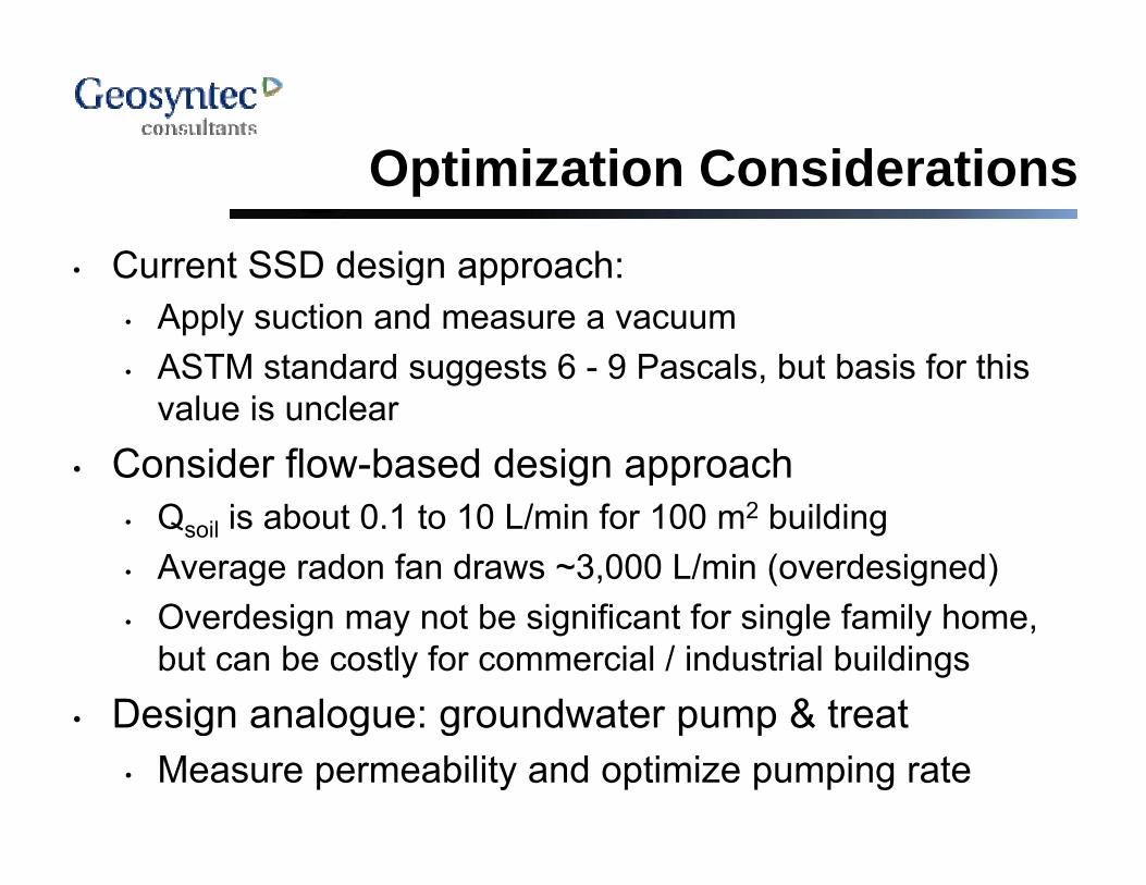
• Current SSD design approach:Current SSD design approach:• Apply suction and measure a vacuum• ASTM standard suggests 6 - 9 Pascals, but basis for this
value is unclear• Consider flow-based design approach
• Qsoil is about 0.1 to 10 L/min for 100 m2 building• Average radon fan draws ~3,000 L/min (overdesigned)
O d i t b i ifi t f i l f il h• Overdesign may not be significant for single family home, but can be costly for commercial / industrial buildings
• Design analogue: groundwater pump & treat• Design analogue: groundwater pump & treat• Measure permeability and optimize pumping rate
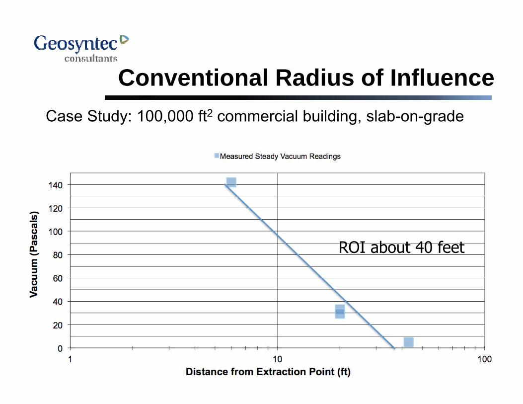
Conventional Radius of InfluenceConventional Radius of InfluenceCase Study: 100,000 ft2 commercial building, slab-on-grade
ROI about 40 feet
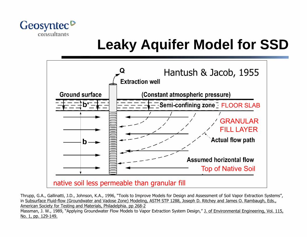
Leaky Aquifer Model for SSDLeaky Aquifer Model for SSD
Hantush & Jacob 1955
FLOOR SLAB
Hantush & Jacob, 1955
FLOOR SLAB
GRANULARFILL LAYER
Top of Native Soil
native soil less permeable than granular fill
Thrupp, G.A., Gallinatti, J.D., Johnson, K.A., 1996, “Tools to Improve Models for Design and Assessment of Soil Vapor Extraction Systems”, in Subsurface Fluid-flow (Groundwater and Vadose Zone) Modeling, ASTM STP 1288, Joseph D. Ritchey and James O. Rambaugh, Eds., American Society for Testing and Materials, Philadelphia. pp 268-2Massman, J. W., 1989, “Applying Groundwater Flow Models to Vapor Extraction System Design,” J. of Environmental Engineering, Vol. 115, No. 1, pp. 129-149.
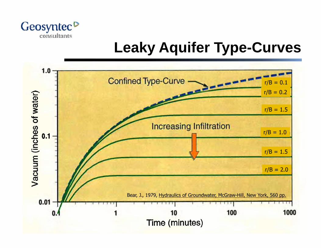
Leaky Aquifer Type CurvesLeaky Aquifer Type-Curves
r/B = 0.1
r/B = 0.2
r/B 1 5r/B = 1.5
r/B = 1.0
r/B = 1.5
r/B = 2.0
Bear, J., 1979, Hydraulics of Groundwater, McGraw-Hill, New York, 560 pp.
r/B 2.0
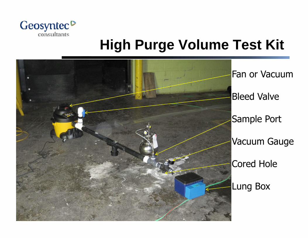
High Purge Volume Test KitHigh Purge Volume Test Kit
Fan or VacuumFan or Vacuum
Bleed Valve
Sample Port
Vacuum Gauge
Cored HoleCored Hole
Lung Box
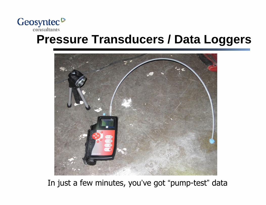
Pressure Transducers / Data LoggersPressure Transducers / Data Loggers
In just a few minutes, you’ve got “pump-test” data
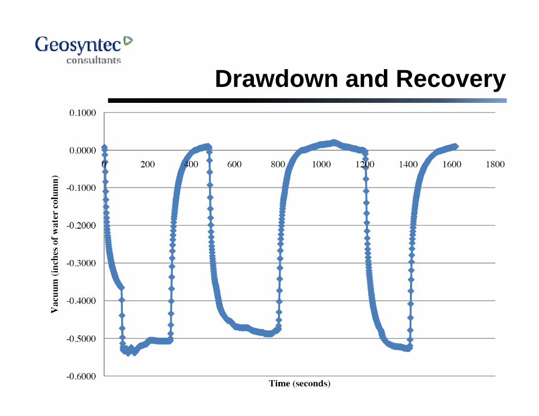
Drawdown and RecoveryDrawdown and Recovery
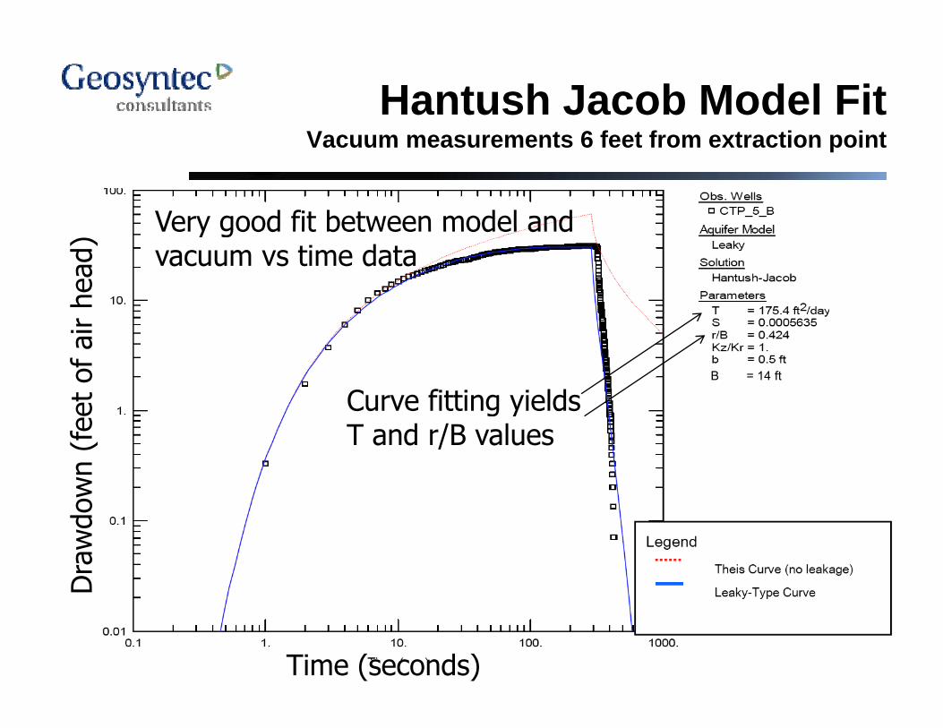
Hantush Jacob Model FitV t 6 f t f t ti i tVacuum measurements 6 feet from extraction point
Very good fit between model and
r he
ad) Very good fit between model and
vacuum vs time data
et o
f ai
r
Curve fitting yieldsB = 14 ft
own
(fee
Curve fitting yields T and r/B values
Dra
wdo
Time (seconds)
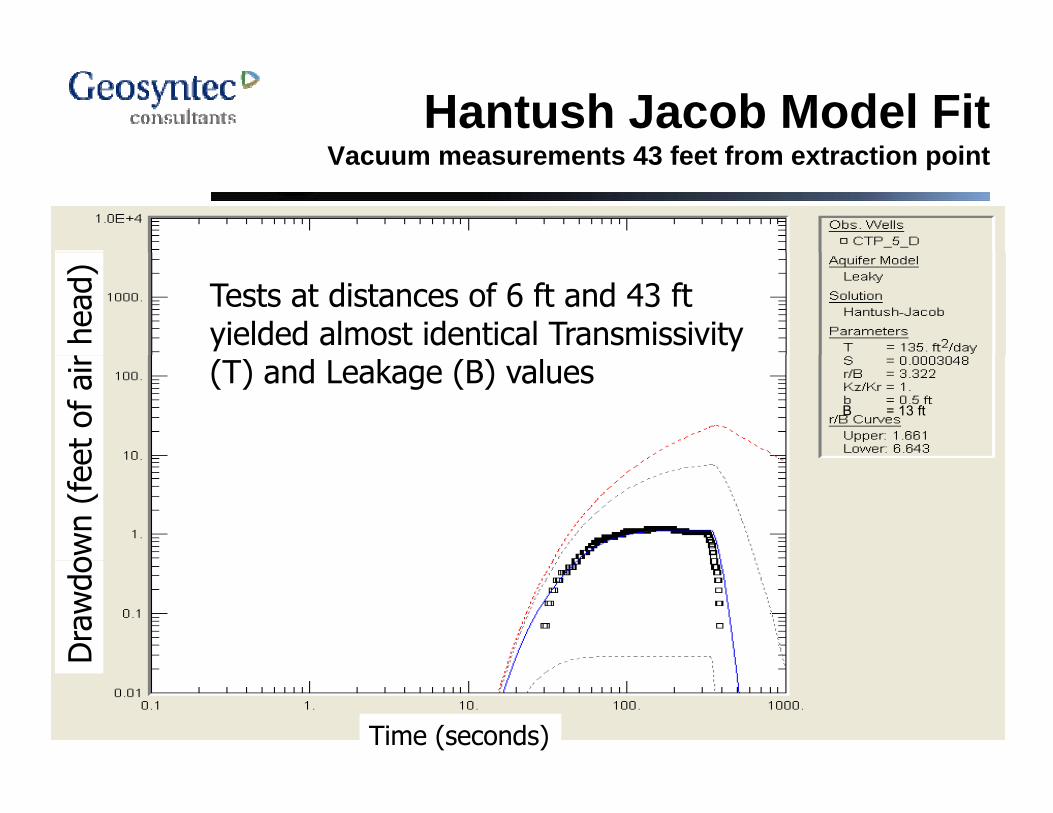
Hantush Jacob Model FitV t 43 f t f t ti i tVacuum measurements 43 feet from extraction point
r he
ad)
Tests at distances of 6 ft and 43 ft yielded almost identical Transmissivity
et o
f ai
r (T) and Leakage (B) values B = 13 ft
own
(fee
Dra
wdo
Time (seconds)
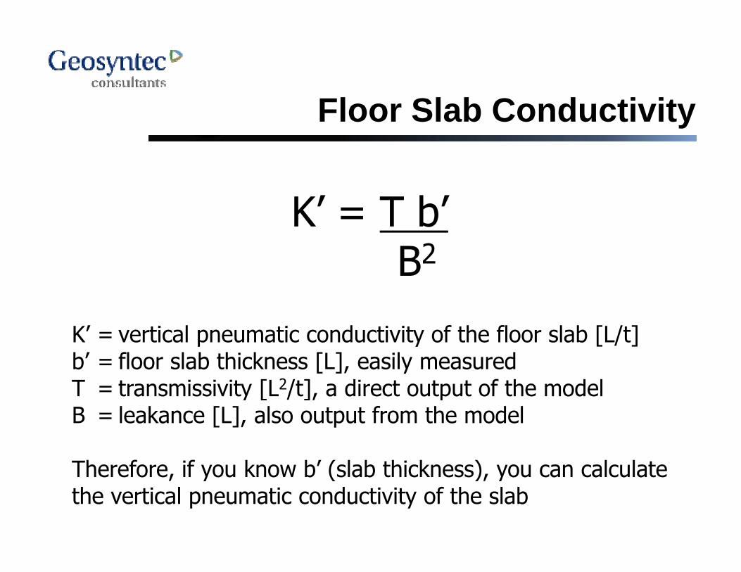
Floor Slab ConductivityFloor Slab Conductivity
K’ = T b’B2B2
K’ = vertical pneumatic conductivity of the floor slab [L/t]b’ = floor slab thickness [L], easily measuredT = transmissivity [L2/t], a direct output of the modelT transmissivity [L /t], a direct output of the modelB = leakance [L], also output from the model
Therefore if you know b’ (slab thickness) you can calculateTherefore, if you know b (slab thickness), you can calculate the vertical pneumatic conductivity of the slab
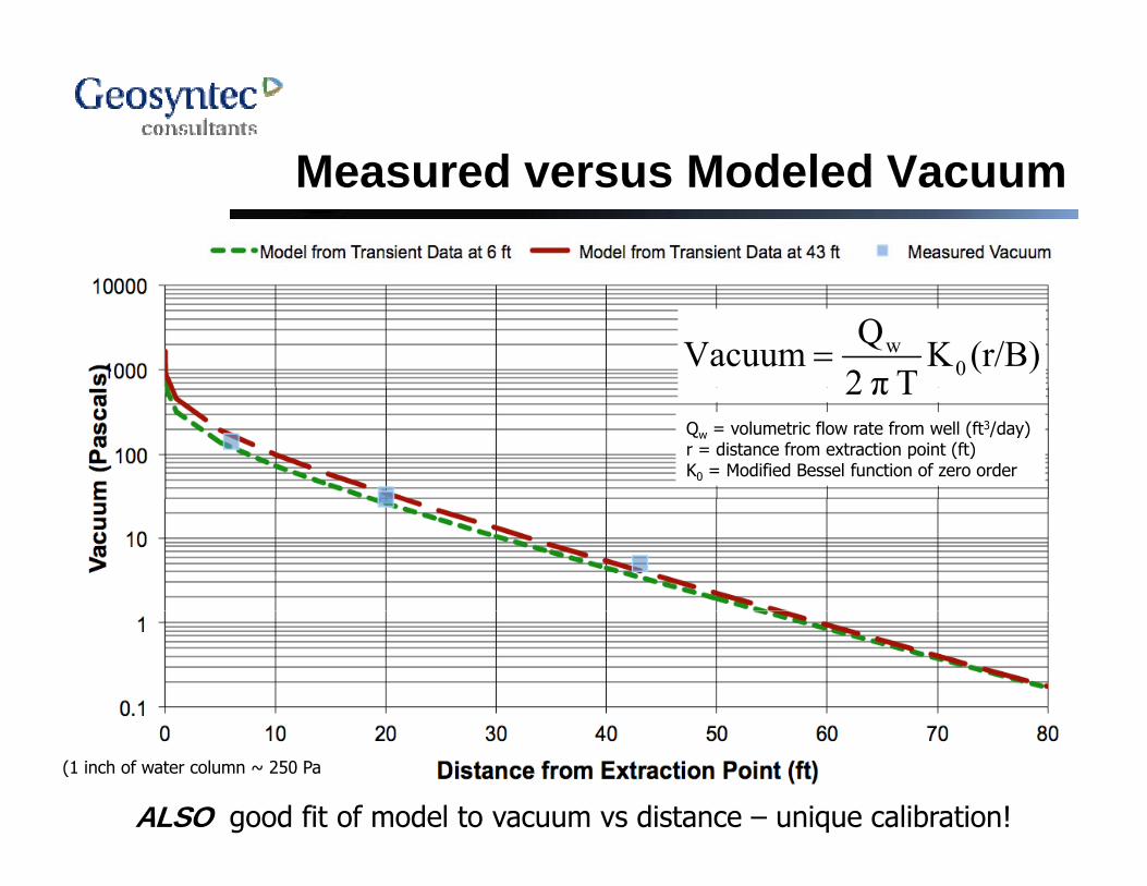
Measured versus Modeled VacuumMeasured versus Modeled Vacuum
(r/B)KTπ2
QVacuum 0wTπ2
Qw = volumetric flow rate from well (ft3/day)r = distance from extraction point (ft)K0 = Modified Bessel function of zero order
ALSO good fit of model to vacuum vs distance – unique calibration!
(1 inch of water column ~ 250 Pa
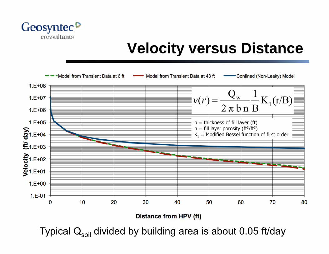
Velocity versus DistanceVelocity versus Distance
(r/B)KB1
nbπ2Q)( 1
wrvBnbπ2
b = thickness of fill layer (ft)n = fill layer porosity (ft3/ft3)K1 = Modified Bessel function of first order
Typical Qsoil divided by building area is about 0.05 ft/day
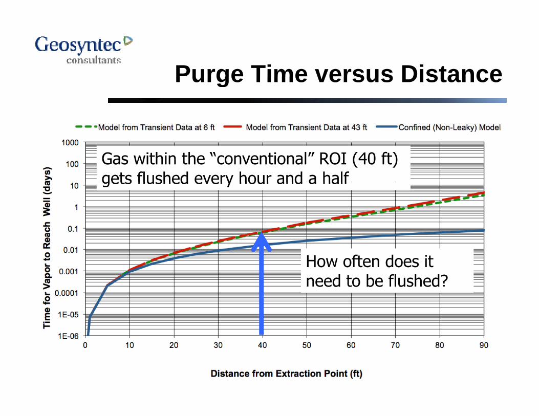
Purge Time versus DistancePurge Time versus Distance
Gas within the “conventional” ROI (40 ft) gets flushed every hour and a halfgets flushed every hour and a half
How often does it need to be flushed?eed to be us ed
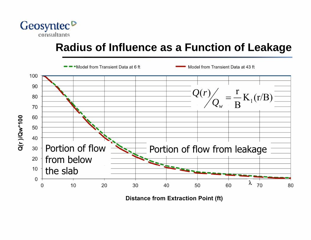
R di f I fl F ti f L kRadius of Influence as a Function of Leakage
(r/B)KBr)(
1QrQ
BwQ
Portion of flow from leakagePortion of flow from below the slab
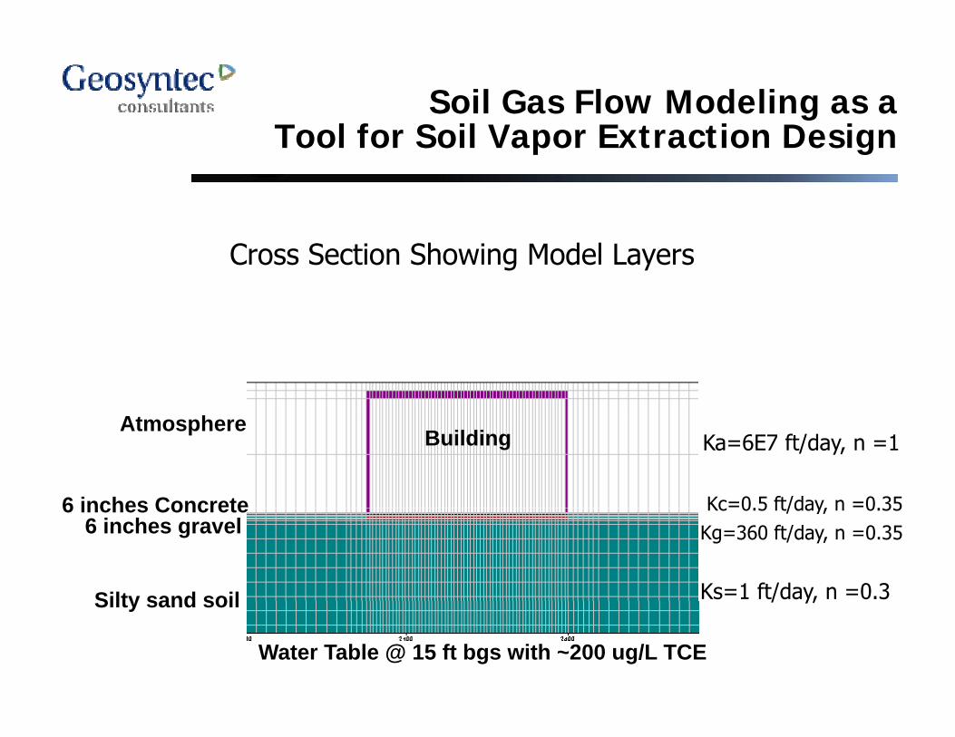
Soil Gas Flow Modeling as a Tool for Soil Vapor Extraction DesignTool for Soil Vapor Extraction Design
Cross Section Showing Model Layers
Atmosphere Building Ka=6E7 ft/day, n =1
Kc=0.5 ft/day, n =0.356 inches Concrete
Ks=1 ft/day, n =0.3
Kg=360 ft/day, n =0.35
Silty sand soil
6 inches gravelKc 0.5 ft/day, n 0.356 inches Concrete
Water Table @ 15 ft bgs with ~200 ug/L TCE
/ y,Silty sand soil
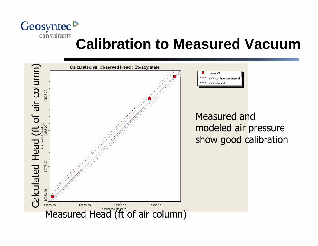
Calibration to Measured VacuumCalibration to Measured Vacuumm
n)ai
r co
lum
Measured and modeled air pressure show good calibration
(ft
of a
show good calibration
ed H
ead
alcu
late
Ca
Measured Head (ft of air column)
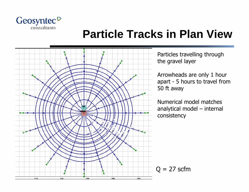
Particle Tracks in Plan ViewParticle Tracks in Plan ViewParticles travelling through th l lthe gravel layer
Arrowheads are only 1 hour apart - 5 hours to travel from p50 ft away
Numerical model matches analytical model internalanalytical model – internal consistency
Q = 27 scfm
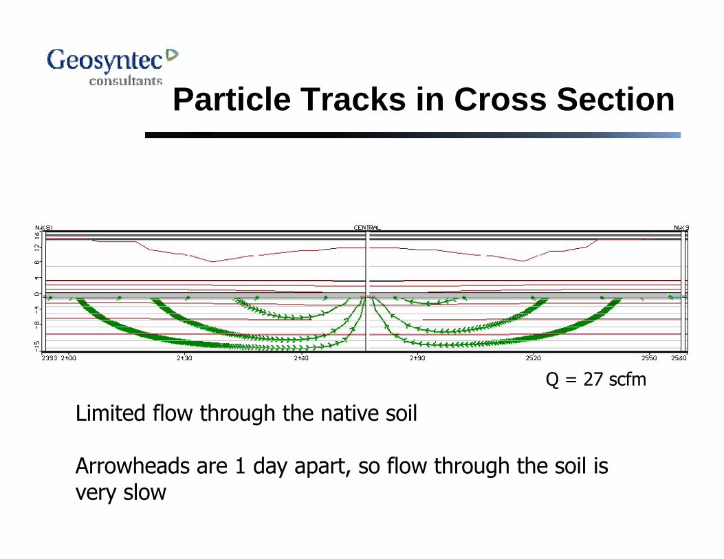
Particle Tracks in Cross SectionParticle Tracks in Cross Section
Q = 27 scfm
Limited flow through the native soil
Q 27 scfm
Arrowheads are 1 day apart, so flow through the soil is very slow
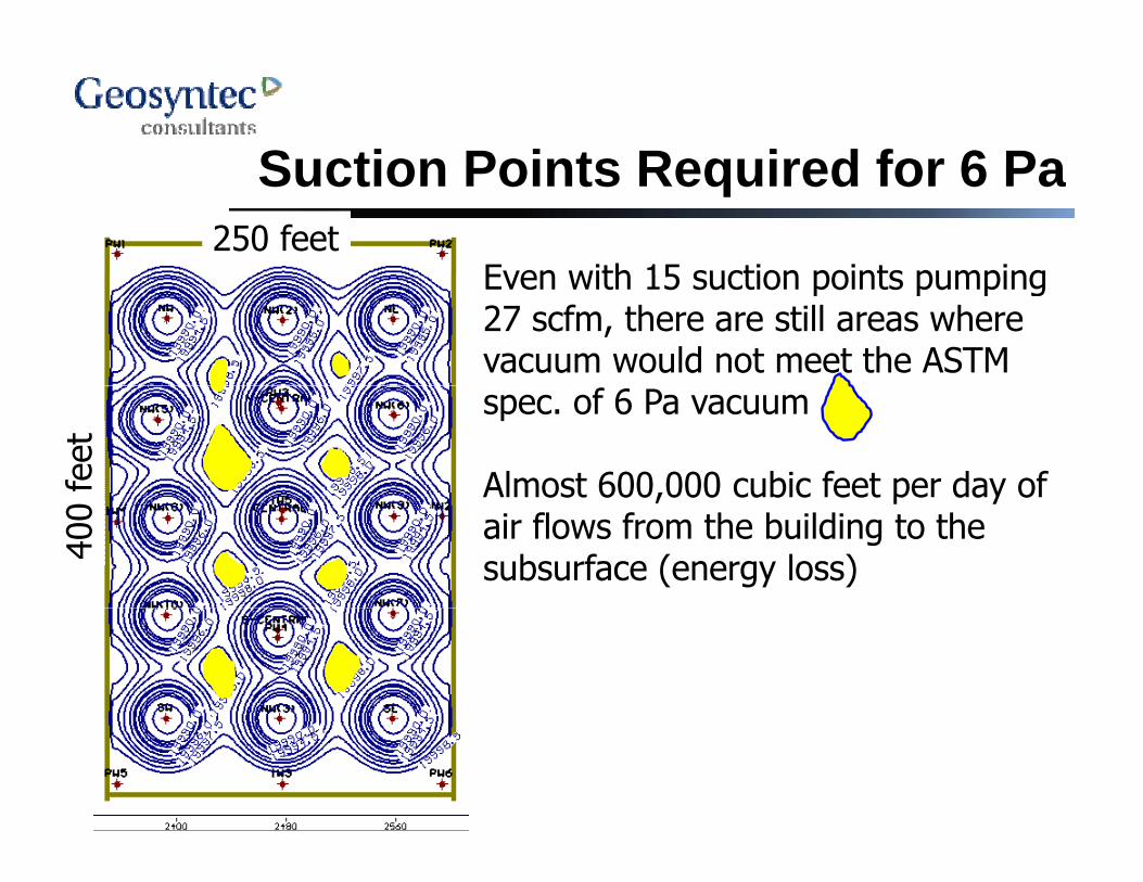
Suction Points Required for 6 PaSuction Points Required for 6 Pa
Even with 15 suction points pumping250 feet
Even with 15 suction points pumping 27 scfm, there are still areas where vacuum would not meet the ASTM spec. of 6 Pa vacuum
Almost 600,000 cubic feet per day offeet
Almost 600,000 cubic feet per day of air flows from the building to the subsurface (energy loss)40
0
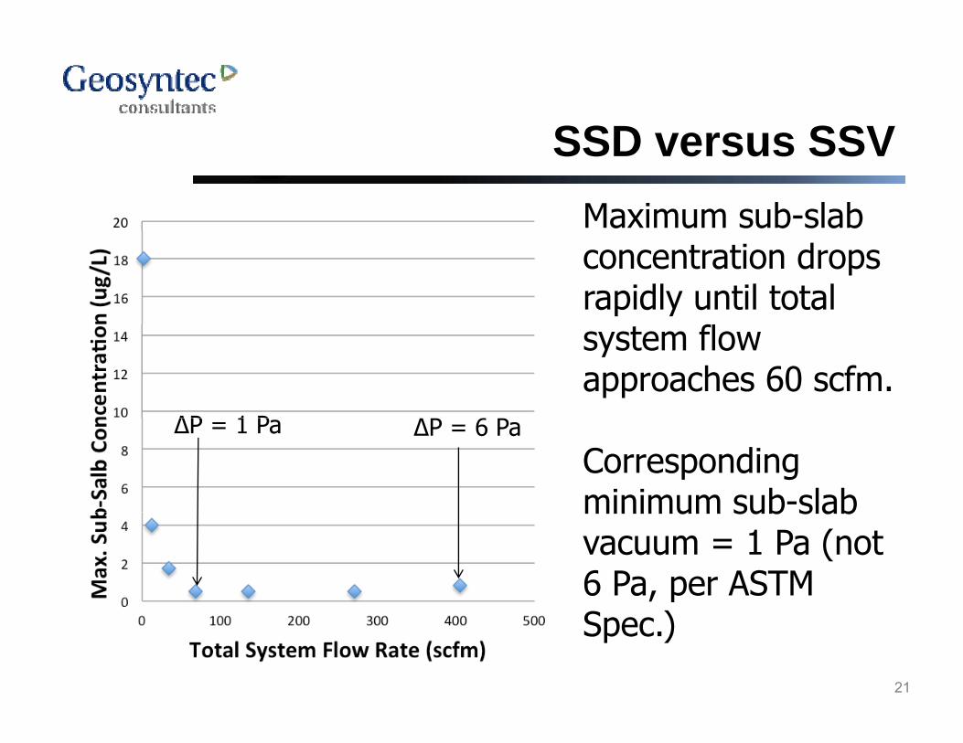
SSD versus SSVSSD versus SSVMaximum sub-slab concentration drops rapidly until total
flsystem flow approaches 60 scfm.
ΔP 1 P ΔP 6 PCorresponding minimum sub-slab
ΔP = 1 Pa ΔP = 6 Pa
minimum sub slab vacuum = 1 Pa (not 6 Pa, per ASTM
21
Spec.)
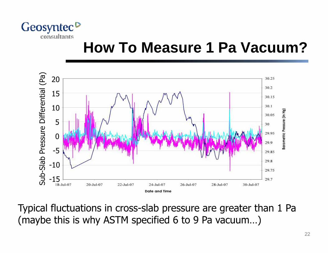
How To Measure 1 Pa Vacuum?How To Measure 1 Pa Vacuum?
20Pa)
10
15
20
eren
tial (
P
5
0
0 ssur
e D
iffe
-5
-10
b-Sl
ab P
res
-15 Sub
Typical fluctuations in cross slab pressure are greater than 1 Pa
22
Typical fluctuations in cross-slab pressure are greater than 1 Pa (maybe this is why ASTM specified 6 to 9 Pa vacuum…)
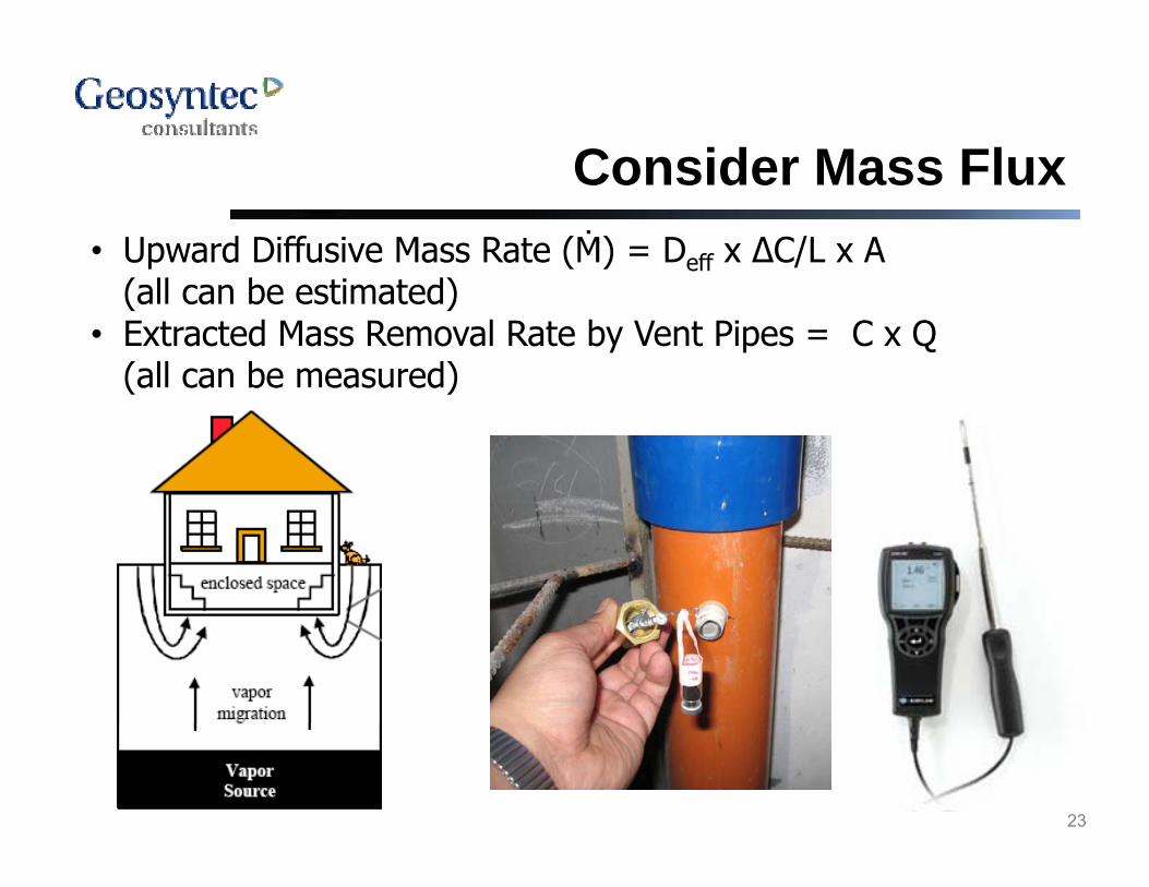
Consider Mass FluxConsider Mass Flux• Upward Diffusive Mass Rate (Ṁ) = Deff x ΔC/L x A
(all can be estimated)• Extracted Mass Removal Rate by Vent Pipes = C x Q
(all can be measured)(a ca be easu ed)
23
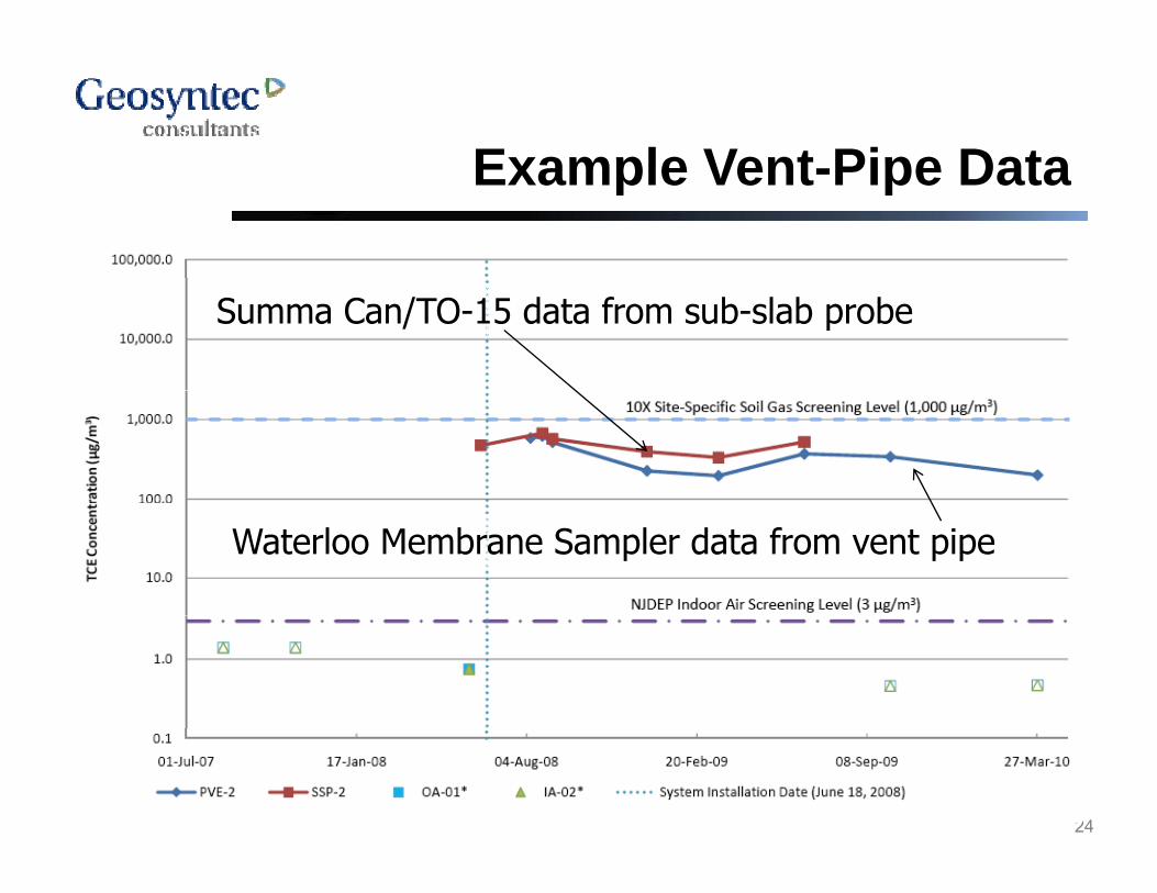
Example Vent Pipe DataExample Vent-Pipe Data
Summa Can/TO-15 data from sub-slab probe
Waterloo Membrane Sampler data from vent pipe
24
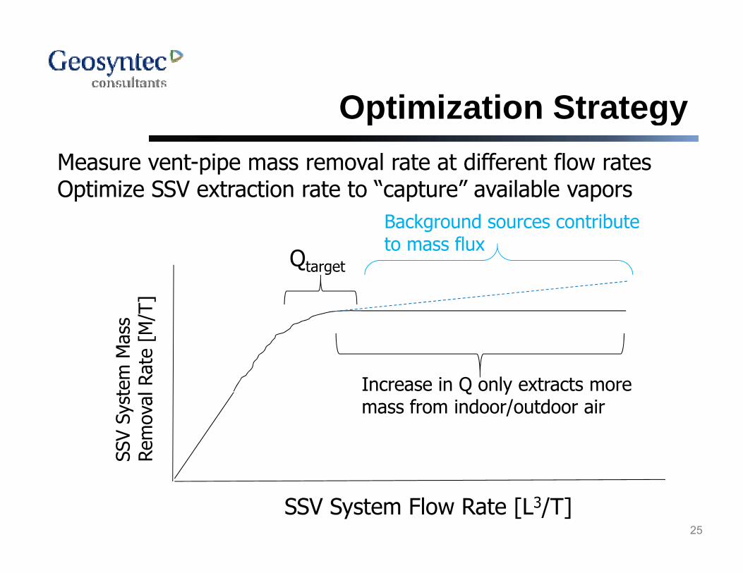
Optimization StrategyOptimization StrategyMeasure vent-pipe mass removal rate at different flow ratesOptimize SSV extraction rate to “capture” available vapors
Q
Background sources contribute to mass flux
s M/T
]
Qtargetto mass flux
tem
Mas
sl R
ate
[M
Increase in Q only extracts more
SSV
Syst
Rem
ova mass from indoor/outdoor air
25
SSV System Flow Rate [L3/T]
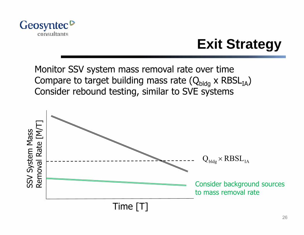
Exit StrategyExit StrategyMonitor SSV system mass removal rate over timeyCompare to target building mass rate (Qbldg x RBSLIA)Consider rebound testing, similar to SVE systems
s M/T
]st
em M
asal
Rat
e [M
IAbldg RBSLQ
SSV
Sys
Rem
ova IAbldgQ
Consider background sources to mass removal rate
26
Time [T]
to mass removal rate
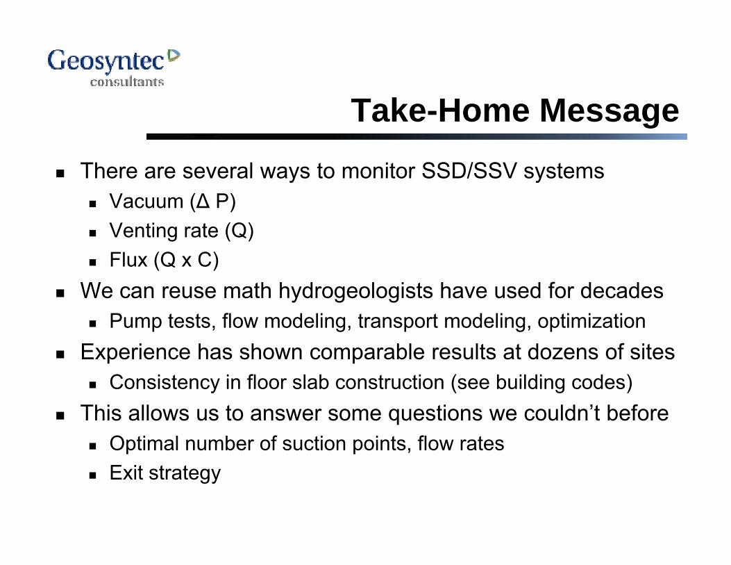
Take Home Message There are several ways to monitor SSD/SSV systems
Take-Home Message There are several ways to monitor SSD/SSV systems
Vacuum (Δ P) Venting rate (Q) Flux (Q x C)
We can reuse math hydrogeologists have used for decadesPump tests flow modeling transport modeling optimization Pump tests, flow modeling, transport modeling, optimization
Experience has shown comparable results at dozens of sites Consistency in floor slab construction (see building codes)y ( g )
This allows us to answer some questions we couldn’t before Optimal number of suction points, flow rates Exit strategy