POINT CLOUD STORAGE AND ACCESS ON A GLOBAL SCALE - DTIC

POINT CLOUD STORAGE AND ACCESS ON A GLOBAL SCALE

JANUARY 2015

INTERIM TECHNICAL REPORT

APPROVED FOR PUBLIC RELEASE; DISTRIBUTION UNLIMITED

STINFO COPY

AIR FORCE RESEARCH LABORATORY INFORMATION DIRECTORATE

AFRL-RI-RS-TR-2015-020

UNITED STATES AIR FORCE ROME, NY 13441 AIR FORCE MATERIEL COMMAND

NOTICE AND SIGNATURE PAGE

Using Government drawings, specifications, or other data included in this document for any purpose other than Government procurement does not in any way obligate the U.S. Government. The fact that the Government formulated or supplied the drawings, specifications, or other data does not license the holder or any other person or corporation; or convey any rights or permission to manufacture, use, or sell any patented invention that may relate to them.

This report was cleared for public release by the 88th ABW, Wright-Patterson AFB Public Affairs Office and is available to the general public, including foreign nationals. Copies may be obtained from the Defense Technical Information Center (DTIC) (http://www.dtic.mil).

AFRL-RI-RS-TR-2015-020 HAS BEEN REVIEWED AND IS APPROVED FOR PUBLICATION IN ACCORDANCE WITH ASSIGNED DISTRIBUTION STATEMENT.

FOR THE DIRECTOR:

/ S / JULIE BRICHACEK Chief, Information Systems Division

/ S / ASHER D. SINCLAIRChief, Resilient Synchronized Systems BranchInformation Systems Division Information Directorate

This report is published in the interest of scientific and technical information exchange, and its publication does not constitute the Government’s approval or disapproval of its ideas or findings.

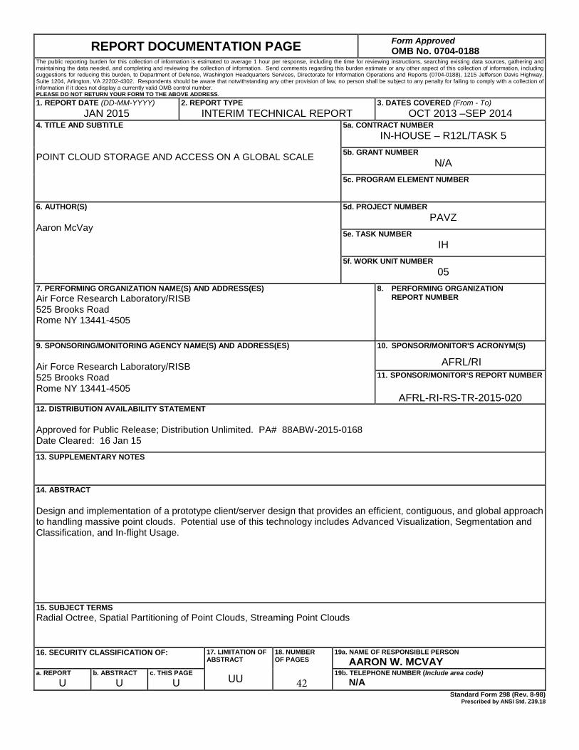
REPORT DOCUMENTATION PAGE Form Approved OMB No. 0704-0188

The public reporting burden for this collection of information is estimated to average 1 hour per response, including the time for reviewing instructions, searching existing data sources, gathering and maintaining the data needed, and completing and reviewing the collection of information. Send comments regarding this burden estimate or any other aspect of this collection of information, including suggestions for reducing this burden, to Department of Defense, Washington Headquarters Services, Directorate for Information Operations and Reports (0704-0188), 1215 Jefferson Davis Highway, Suite 1204, Arlington, VA 22202-4302. Respondents should be aware that notwithstanding any other provision of law, no person shall be subject to any penalty for failing to comply with a collection of information if it does not display a currently valid OMB control number. PLEASE DO NOT RETURN YOUR FORM TO THE ABOVE ADDRESS. 1. REPORT DATE (DD-MM-YYYY)

JAN 2015 2. REPORT TYPE

INTERIM TECHNICAL REPORT 3. DATES COVERED (From - To)

OCT 2013 –SEP 2014 4. TITLE AND SUBTITLE

POINT CLOUD STORAGE AND ACCESS ON A GLOBAL SCALE

5a. CONTRACT NUMBER IN-HOUSE – R12L/TASK 5

5b. GRANT NUMBER N/A

5c. PROGRAM ELEMENT NUMBER

6. AUTHOR(S)

Aaron McVay

5d. PROJECT NUMBER PAVZ

5e. TASK NUMBER IH

5f. WORK UNIT NUMBER 05

7. PERFORMING ORGANIZATION NAME(S) AND ADDRESS(ES)Air Force Research Laboratory/RISB 525 Brooks Road Rome NY 13441-4505

8. PERFORMING ORGANIZATIONREPORT NUMBER

9. SPONSORING/MONITORING AGENCY NAME(S) AND ADDRESS(ES)

Air Force Research Laboratory/RISB 525 Brooks Road Rome NY 13441-4505

10. SPONSOR/MONITOR'S ACRONYM(S)

AFRL/RI 11. SPONSOR/MONITOR’S REPORT NUMBER

AFRL-RI-RS-TR-2015-020 12. DISTRIBUTION AVAILABILITY STATEMENT

Approved for Public Release; Distribution Unlimited. PA# 88ABW-2015-0168 Date Cleared: 16 Jan 15 13. SUPPLEMENTARY NOTES

14. ABSTRACT

Design and implementation of a prototype client/server design that provides an efficient, contiguous, and global approach to handling massive point clouds. Potential use of this technology includes Advanced Visualization, Segmentation and Classification, and In-flight Usage.

15. SUBJECT TERMSRadial Octree, Spatial Partitioning of Point Clouds, Streaming Point Clouds

16. SECURITY CLASSIFICATION OF: 17. LIMITATION OF ABSTRACT

UU

18. NUMBEROF PAGES

19a. NAME OF RESPONSIBLE PERSON AARON W. MCVAY

a. REPORTU

b. ABSTRACTU

c. THIS PAGEU

19b. TELEPHONE NUMBER (Include area code) N/A

Standard Form 298 (Rev. 8-98) Prescribed by ANSI Std. Z39.18

42

Table of Contents

1.0 Summary ........................................................................................................................................... 1

2.0 Introduction ...................................................................................................................................... 2

3.0 Methods, Assumptions, and Procedures .......................................................................................... 5

3.1. Open Source Software .................................................................................................................. 5

3.2. Coordinate System(s) .................................................................................................................... 5

3.3. Data Storage / Spatial Acceleration .............................................................................................. 6

3.4. Data Ingestion ............................................................................................................................. 10

3.5. Data Access by Geometry ........................................................................................................... 14

3.5.1. 2D Polygon .......................................................................................................................... 15

3.5.2. 3D Frustum .......................................................................................................................... 17

3.6. Streaming Client(s) / Server ........................................................................................................ 20

3.6.1. Easy Socket (C++/JAVA) Messages ...................................................................................... 21

3.6.2. Point Server Prototype ........................................................................................................ 21

3.6.3. JView World Client .............................................................................................................. 23

3.6.4. JDAR Client .......................................................................................................................... 25

3.6.5. WebGL Client (VISRIDER Task #6) ....................................................................................... 26

3.7. Performance Characteristics ....................................................................................................... 27

3.7.1. Ingestion .............................................................................................................................. 27

3.7.2. Access .................................................................................................................................. 28

4.0 Results and Discussion .................................................................................................................... 31

5.0 Conclusions ..................................................................................................................................... 33

6.0 References ...................................................................................................................................... 34

List of Symbols, Abbreviations, and Acronyms ........................................................................................... 35

i

List of Figures

Figure 1 - UTM Zone 18 (NGA, 2013) ............................................................................................................ 2 Figure 2 - WGS84 EC Coordinate System (NOAA, 2007) ............................................................................... 2 Figure 3 - 2008 Democratic National Convention (DNC) LiDAR Coverage Map for Denver, CO .................. 3 Figure 4 - Quick Terrain Modeler Displaying Denver DNC Dataset of Denver Airport (Applied Imagery, 2013) ............................................................................................................................................................. 4 Figure 5- Cylindrical (Flat Earth) Representation of Globe Partitioned by 2D Quadtree in Latitude and Longitude ...................................................................................................................................................... 7 Figure 6 - Spherical (Round Earth / WGS84) Representation of Globe Partitioned by 2D Quadtree in Latitude and Longitude ................................................................................................................................. 7 Figure 7 - 2D Geographic Partitioning with a Quadtree ............................................................................... 8 Figure 8 - Globe Partitioned by 3D Octree in WGS84 ECEF .......................................................................... 9 Figure 9 - High Level Pseudo code for Data Ingestion ................................................................................ 12 Figure 10 - Single Top Level (0) Node Contents .......................................................................................... 13 Figure 11 - Top Level (0) Node Divided into 3 Children .............................................................................. 13 Figure 12 – Example Octree Representation of Sandia Mountains East of Albuquerque, NM .................. 14 Figure 13 – Ideal Leaf Node 2D Polygon Intersection Test ......................................................................... 16 Figure 14 - 2D Polygon and Edge Cells (left), Pruned Results (bottom right), Non-pruned Results (upper right) ............................................................................................................................................................ 17 Figure 15 - 3D Frustum................................................................................................................................ 18 Figure 16 - Cells that Overlap Frustum ....................................................................................................... 18 Figure 17- 3D Frustum of Denver Airport (Not-Pruned) ............................................................................. 19 Figure 18 - 3D Frustum of Denver Airport (Pruned) ................................................................................... 20 Figure 19 - JView World with DARPA URGENT Point Cloud Data for a Sub Region of Ottawa, Canada ..... 23 Figure 20 - JView World with Point Data for Sub Region of Beale, AFB ..................................................... 24 Figure 21 – JDAR Toolkit Displaying LiDAR Data for Beale, AFB Showing KC-135s Parked on Northern Tarmac ........................................................................................................................................................ 25 Figure 22 – Chrome Web Browser (WebGL) with DARPA URGENT Point Data for Sub Region of Ottawa, Canada ........................................................................................................................................................ 26 Figure 23 - 3D Frustum Request as Seen on Computer Screen .................................................................. 29 Figure 24 - 3D Frustum Request after Zoom Out (Not-Pruned) ................................................................. 30 Figure 25 - Point Cloud Colored by Imagery of Sandia Mountains East of Albuquerque, NM ................... 32

ii

List of Tables

Table 1 - Global Octree Resolution by Level ............................................................................................... 11 Table 2 - Point Cloud Server Configure State Messages ............................................................................. 21 Table 3 - Point Cloud Server Queries .......................................................................................................... 22 Table 4 - Performance Test(s) System Configuration ................................................................................. 27 Table 5 – Summary of Ingestion Performance Statistics ............................................................................ 27 Table 6 - Estimated Time to Ingest 1 Trillion Points ................................................................................... 27 Table 7 - 2D Polygon Query Client/Server Performance Statistics (Not-Pruned) ....................................... 28 Table 8 - 2D Polygon Query Client/Server Performance Statistics (Pruned) .............................................. 28 Table 9 - 3D Frustum Query Client/Server Performance Statistics (Not-Pruned) ...................................... 30

iii

1.0 Summary

Point Cloud data is a collection of sampled points representing the three dimensional (X, Y, Z) surface coordinates of an object typically generated by a scanning device or computer simulation. Light Detection and Ranging (LiDAR) systems are one example of geospatial point cloud generation using a range finding LASER to perform high resolution target mapping from aircraft or other vehicles.

Modern LiDAR sensors generate Terabytes of point cloud data resulting in datasets too large for the current state of the art commercial software to Process, Exploit, Disseminate (PED), and visualize. LiDAR PED efforts can take weeks to months requiring complex and labor intensive processing to create data products that have been altered from their original raw forms through sampling or interpolation; resulting in a loss of potentially critical information.

The primary limitations of typical commercial LiDAR software applications are: 1) suitability only to small geographic regions, 2) inability to process data that isn’t stored locally, and 3) constrained by the amount of available RAM in the system. A service based approach needed to be developed to allow applications to utilize a streaming metaphor in order to access these massive datasets on a global scale. This approach eliminates the requirement for workstations to store Terabytes of data and permits sharing of intermediate products and visualizations.

The goal of this effort was an initial design and implementation of a prototype client/server design that provides an efficient, contiguous, and global approach to handling massive point clouds. Potential use of this technology includes Advanced Visualization, Object Segmentation, Classification, and Inflight Usage.

Technologies developed in this effort include:

• Development of an advanced data structure for storage and access of point cloud data on aglobal scale that utilizes the WGS84 Earth Centered Earth Fixed coordinate systems which is notlimited to small geographic regions

• Development of an initial set of prototypes demonstrating streaming point cloud data tomultiple categories of clients.

APPROVED FOR PUBLIC RELEASE; DISTRIBUTION UNLIMITED 1

2.0 Introduction

Modern LiDAR sensors generate Terabytes of point cloud data resulting in datasets too large for the current state of the art commercial software to Process, Exploit, Disseminate (PED), and visualize. LiDAR PED efforts can take weeks to months requiring complex and labor intensive processing to create data products that have been altered from their original raw forms through sampling or interpolation; resulting in a loss of potentially critical information.

The primary limitations of typical commercial LiDAR software applications are: 1) suitability only to small geographic regions, 2) inability to process data that isn’t stored locally, and 3) constrained by the amount of available RAM in the system. A service based approach needed to be developed to allow applications to utilize a streaming metaphor in order to access these massive datasets on a global scale. This approach eliminates the requirement for workstations to store terabytes of data and permits sharing of intermediate products and visualizations.

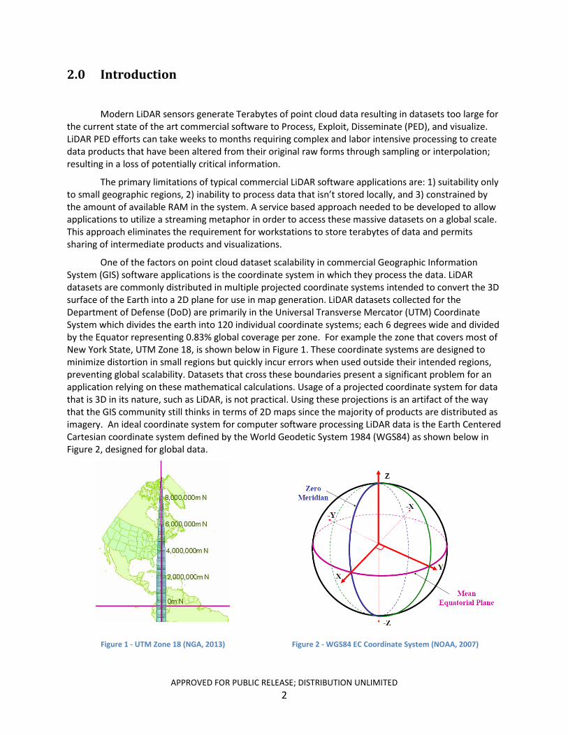
One of the factors on point cloud dataset scalability in commercial Geographic Information System (GIS) software applications is the coordinate system in which they process the data. LiDAR datasets are commonly distributed in multiple projected coordinate systems intended to convert the 3D surface of the Earth into a 2D plane for use in map generation. LiDAR datasets collected for the Department of Defense (DoD) are primarily in the Universal Transverse Mercator (UTM) Coordinate System which divides the earth into 120 individual coordinate systems; each 6 degrees wide and divided by the Equator representing 0.83% global coverage per zone. For example the zone that covers most of New York State, UTM Zone 18, is shown below in Figure 1. These coordinate systems are designed to minimize distortion in small regions but quickly incur errors when used outside their intended regions, preventing global scalability. Datasets that cross these boundaries present a significant problem for an application relying on these mathematical calculations. Usage of a projected coordinate system for data that is 3D in its nature, such as LiDAR, is not practical. Using these projections is an artifact of the way that the GIS community still thinks in terms of 2D maps since the majority of products are distributed as imagery. An ideal coordinate system for computer software processing LiDAR data is the Earth Centered Cartesian coordinate system defined by the World Geodetic System 1984 (WGS84) as shown below in Figure 2, designed for global data.

Figure 1 - UTM Zone 18 (NGA, 2013) Figure 2 - WGS84 EC Coordinate System (NOAA, 2007)


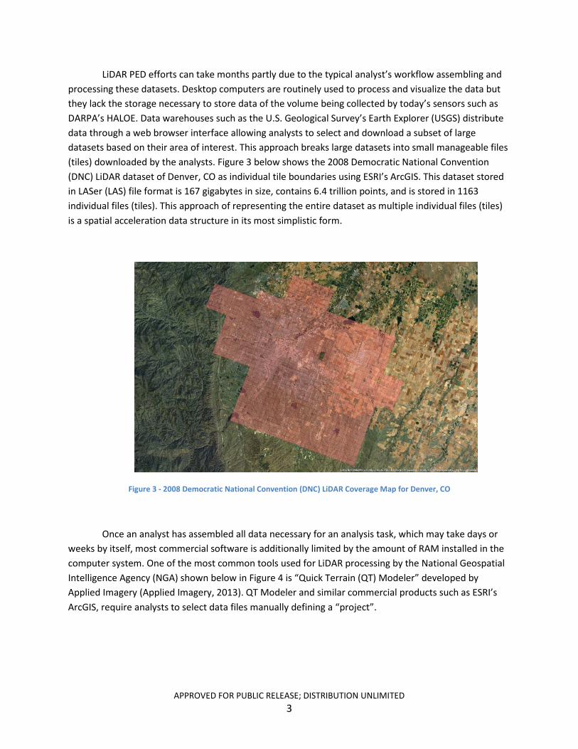
LiDAR PED efforts can take months partly due to the typical analyst’s workflow assembling and processing these datasets. Desktop computers are routinely used to process and visualize the data but they lack the storage necessary to store data of the volume being collected by today’s sensors such as DARPA’s HALOE. Data warehouses such as the U.S. Geological Survey’s Earth Explorer (USGS) distribute data through a web browser interface allowing analysts to select and download a subset of large datasets based on their area of interest. This approach breaks large datasets into small manageable files (tiles) downloaded by the analysts. Figure 3 below shows the 2008 Democratic National Convention (DNC) LiDAR dataset of Denver, CO as individual tile boundaries using ESRI’s ArcGIS. This dataset stored in LASer (LAS) file format is 167 gigabytes in size, contains 6.4 trillion points, and is stored in 1163 individual files (tiles). This approach of representing the entire dataset as multiple individual files (tiles) is a spatial acceleration data structure in its most simplistic form.

Figure 3 - 2008 Democratic National Convention (DNC) LiDAR Coverage Map for Denver, CO

Once an analyst has assembled all data necessary for an analysis task, which may take days or weeks by itself, most commercial software is additionally limited by the amount of RAM installed in the computer system. One of the most common tools used for LiDAR processing by the National Geospatial Intelligence Agency (NGA) shown below in Figure 4 is “Quick Terrain (QT) Modeler” developed by Applied Imagery (Applied Imagery, 2013). QT Modeler and similar commercial products such as ESRI’s ArcGIS, require analysts to select data files manually defining a “project”.


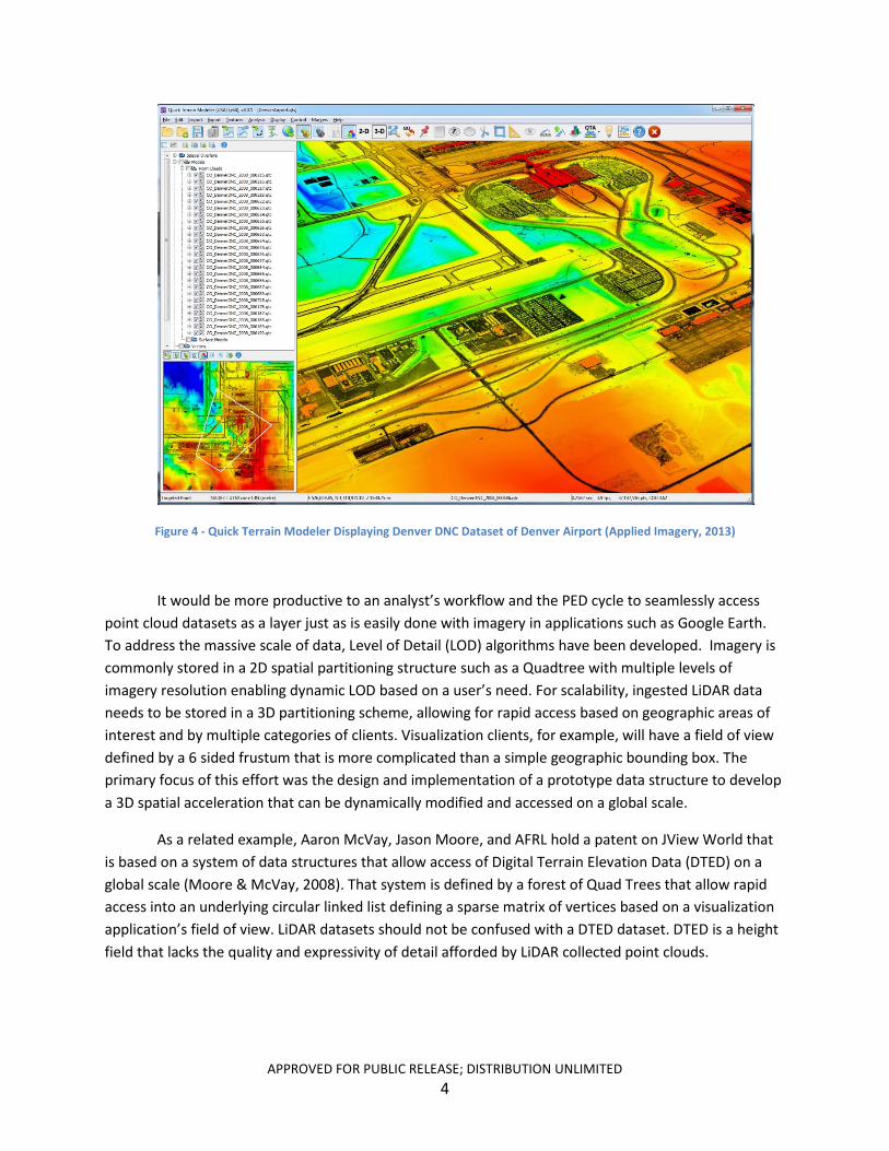
Figure 4 - Quick Terrain Modeler Displaying Denver DNC Dataset of Denver Airport (Applied Imagery, 2013)

It would be more productive to an analyst’s workflow and the PED cycle to seamlessly access point cloud datasets as a layer just as is easily done with imagery in applications such as Google Earth. To address the massive scale of data, Level of Detail (LOD) algorithms have been developed. Imagery is commonly stored in a 2D spatial partitioning structure such as a Quadtree with multiple levels of imagery resolution enabling dynamic LOD based on a user’s need. For scalability, ingested LiDAR data needs to be stored in a 3D partitioning scheme, allowing for rapid access based on geographic areas of interest and by multiple categories of clients. Visualization clients, for example, will have a field of view defined by a 6 sided frustum that is more complicated than a simple geographic bounding box. The primary focus of this effort was the design and implementation of a prototype data structure to develop a 3D spatial acceleration that can be dynamically modified and accessed on a global scale.

As a related example, Aaron McVay, Jason Moore, and AFRL hold a patent on JView World that is based on a system of data structures that allow access of Digital Terrain Elevation Data (DTED) on a global scale (Moore & McVay, 2008). That system is defined by a forest of Quad Trees that allow rapid access into an underlying circular linked list defining a sparse matrix of vertices based on a visualization application’s field of view. LiDAR datasets should not be confused with a DTED dataset. DTED is a height field that lacks the quality and expressivity of detail afforded by LiDAR collected point clouds.


3.0 Methods, Assumptions, and Procedures

3.1. Open Source Software

The bulk of LiDAR data distributed today is in projected coordinate systems using the LASer (LAS) File Format defined by The American Society for Photogrammetry and Remote Sensing (ASPRS, 2013). Due to the potential size of these files they are frequently compressed into the LAZ format. The goal of this project was not to develop file parsers, or to implement coordinate system conversion algorithms and as such, well know open source software libraries were used for these tasks.

Initially, the following libraries were used to parse, decompress, and re-project point cloud datasets using the C++ programming language under various flavors of the Linux operating system;

• libLAS – ASPRS LiDAR data translation toolset http://www.liblas.org/• LASZip – lossless LiDAR compression Library http://www.laszip.org/• PROJ.4 – Cartographic Projections Library http://trac.osgeo.org/proj

LibLAS was developed by multiple organizations including the U.S Army Cold Regions Research and Engineer Laboratory (CRREL), but as of the writing of this report, development and maintenance of libLAS had declining support. CRREL is actively expanding and supporting the Point Data Abstraction Library (PDAL) as the next generation replacement of the libLAS library.

• PDAL – Point Data Abstraction Library http://www.pointcloud.org/

In addition to parsing LAS/LAZ files PDAL contains a workflow pipeline that includes projection, filtering, and spatial partitioning. For this reason near the completion of this effort libLAS was replaced with PDAL for data parsing.

3.2. Coordinate System(s)

One of the factors on point cloud dataset scalability in commercial GIS software applications is the coordinate system in which they process the data. Point Cloud datasets are commonly distributed in multiple projected coordinate systems intended to translate the 3D surface of the Earth onto a 2D plane for use in map generation. LiDAR datasets collected for the Department of Defense (DOD) primarily store their horizontal coordinates in the Universal Transverse Mercator (UTM) System using the NAD83 horizontal datum, and EGM96 or WGS84 for the vertical datum as shown above in Figure 1. Local governments more often use one of the State Plane Coordinate Systems; Texas for example is divided into 5 such coordinate systems. These projected coordinate systems are designed to minimize distortion in small regions but quickly incur errors when used outside their intended regions, preventing global scalability.


Any system design intended to access point cloud datasets spanning large geographic distances should use a coordinate system that is continuous across the entire globe. Storing data in “Geodetic” Latitude/Longitude/Altitude (LLA) coordinates provides a single global coordinate system, but LLA has 3 regions where the coordinate system has discontinuities, specifically at the poles and in the middle of the Pacific Ocean at 180E/180W. Performing analysis in LLA coordinates if your calculation crosses any of these 3 regions creates a challenge; additionally altitude is not in the same units as the horizontal component (Feet or Meters versus degrees).

An ideal coordinate system for computer software processing LiDAR data is the Earth Centered Earth Fixed (ECEF) Cartesian coordinate system defined by the World Geodetic System 1984 (WGS84) as shown above in Figure 2, which is designed for global data. The obvious advantage to ECEF is it’s a continuous Euclidian coordinate system covering the entire globe allowing for mathematical calculations without regions where discontinuities exist. The major disadvantage to this system is the coordinates are not intuitively human interpretable. Due to the size of these point cloud datasets being potentially in the trillions, the ability for a human to manually interpret individual point values does not present a compelling design consideration. It is a trivial set of computations for a computer to re-project a subset of points in a volume that is practical for human inspection.

3.3. Data Storage / Spatial Acceleration

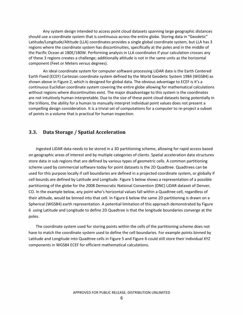
Ingested LiDAR data needs to be stored in a 3D partitioning scheme, allowing for rapid access based on geographic areas of interest and by multiple categories of clients. Spatial acceleration data structures store data in sub regions that are defined by various types of geometric cells. A common partitioning scheme used by commercial software today for point datasets is the 2D Quadtree. Quadtrees can be used for this purpose locally if cell boundaries are defined in a projected coordinate system, or globally if cell bounds are defined by Latitude and Longitude. Figure 5 below shows a representation of a possible partitioning of the globe for the 2008 Democratic National Convention (DNC) LiDAR dataset of Denver, CO. In the example below, any point who’s horizontal values fall within a Quadtree cell, regardless of their altitude, would be binned into that cell. In Figure 6 below the same 2D partitioning is drawn on a Spherical (WGS84) earth representation. A potential limitation of this approach demonstrated by Figure 6 using Latitude and Longitude to define 2D Quadtree is that the longitude boundaries converge at the poles.

The coordinate system used for storing points within the cells of the partitioning scheme does not have to match the coordinate system used to define the cell boundaries. For example points binned by Latitude and Longitude into Quadtree cells in Figure 5 and Figure 6 could still store their individual XYZ components in WGS84 ECEF for efficient mathematical calculations.


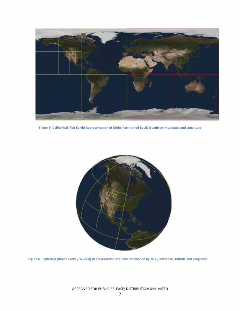
Figure 5- Cylindrical (Flat Earth) Representation of Globe Partitioned by 2D Quadtree in Latitude and Longitude

Figure 6 - Spherical (Round Earth / WGS84) Representation of Globe Partitioned by 2D Quadtree in Latitude and Longitude


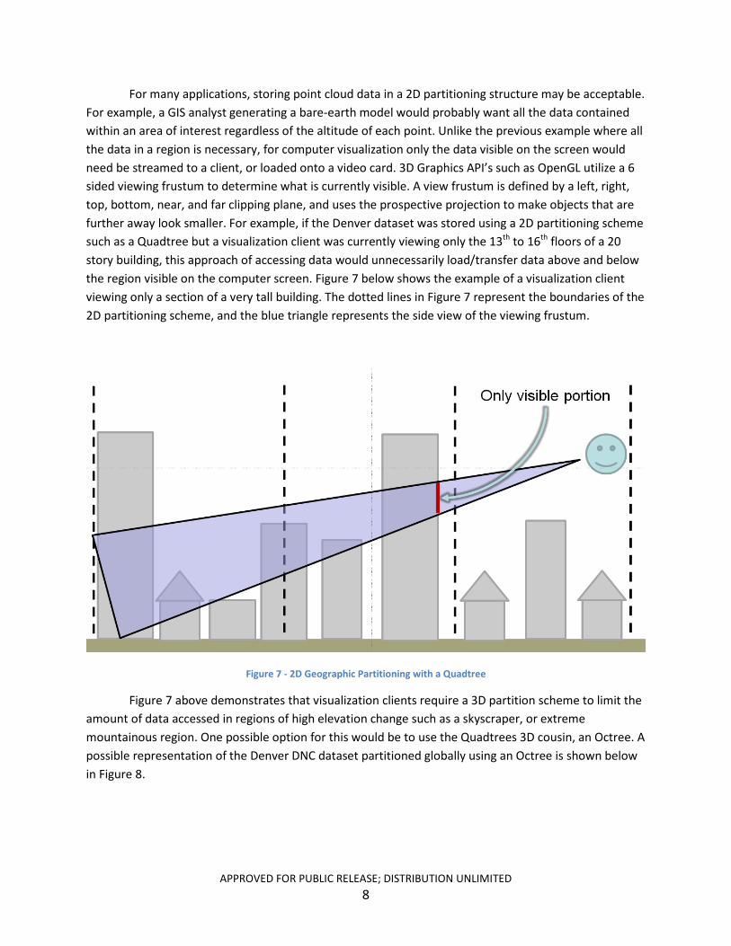
For many applications, storing point cloud data in a 2D partitioning structure may be acceptable. For example, a GIS analyst generating a bare-earth model would probably want all the data contained within an area of interest regardless of the altitude of each point. Unlike the previous example where all the data in a region is necessary, for computer visualization only the data visible on the screen would need be streamed to a client, or loaded onto a video card. 3D Graphics API’s such as OpenGL utilize a 6 sided viewing frustum to determine what is currently visible. A view frustum is defined by a left, right, top, bottom, near, and far clipping plane, and uses the prospective projection to make objects that are further away look smaller. For example, if the Denver dataset was stored using a 2D partitioning scheme such as a Quadtree but a visualization client was currently viewing only the 13th to 16th floors of a 20 story building, this approach of accessing data would unnecessarily load/transfer data above and below the region visible on the computer screen. Figure 7 below shows the example of a visualization client viewing only a section of a very tall building. The dotted lines in Figure 7 represent the boundaries of the 2D partitioning scheme, and the blue triangle represents the side view of the viewing frustum.

Figure 7 - 2D Geographic Partitioning with a Quadtree

Figure 7 above demonstrates that visualization clients require a 3D partition scheme to limit the amount of data accessed in regions of high elevation change such as a skyscraper, or extreme mountainous region. One possible option for this would be to use the Quadtrees 3D cousin, an Octree. A possible representation of the Denver DNC dataset partitioned globally using an Octree is shown below in Figure 8.


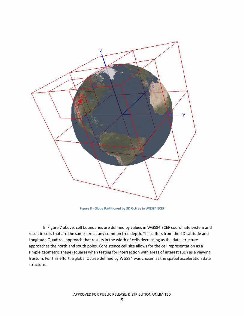
Figure 8 - Globe Partitioned by 3D Octree in WGS84 ECEF

In Figure 7 above, cell boundaries are defined by values in WGS84 ECEF coordinate system and result in cells that are the same size at any common tree depth. This differs from the 2D Latitude and Longitude Quadtree approach that results in the width of cells decreasing as the data structure approaches the north and south poles. Consistence cell size allows for the cell representation as a simple geometric shape (square) when testing for intersection with areas of interest such as a viewing frustum. For this effort, a global Octree defined by WGS84 was chosen as the spatial acceleration data structure.


3.4. Data Ingestion

The intended use of the spatial acceleration structure for this effort was not to partition down to the point level, but rather to create rapidly accessible sub-clouds of manageable size. Each cell in the global Octree is a sub-cloud, or bucket of points. The bucket size was implemented as a configuration setting allowing bucket size to be determined by individual use case.

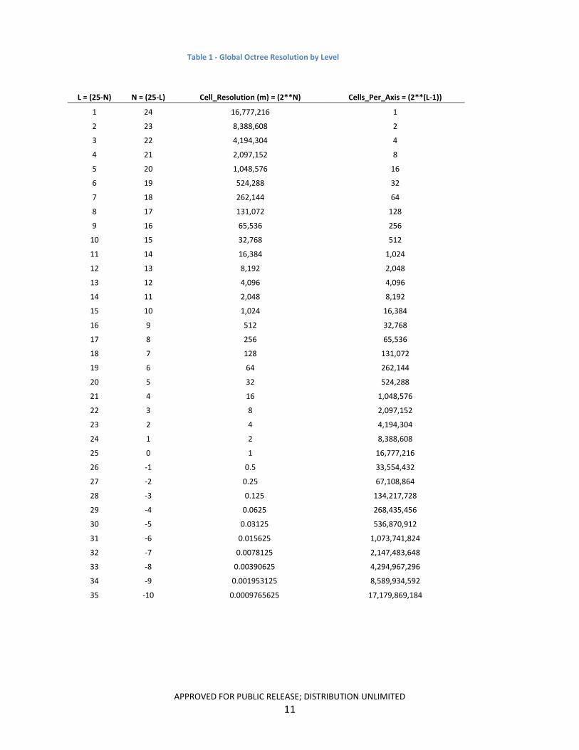
The typical usage of an Octree, or other spatial acceleration structure, is to define its extents based on the extents of the data, then subdivide those extents as the tree divides into children. For this application, it was decided to define any generated Octree based on maximal global extents, regardless of the data extents. The only requirement is that one level of the Octree snapped to exactly 1 meter square cells in WGS84 ECEF. To conserve memory this approach doesn’t create branches that do not contain data, resulting in a sparse tree. There are two clear advantages to this approach; 1) common potential structure simplifies the process of pulling data from different trees, 2) snapping some level to exactly 1 meter makes it possible to define a closed form solution for cell resolution. Level 1 was defined as the top most node and Level 25 as 1 square meter. The number of levels was determined in reverse by calculation of how many levels up from 1 square meter would define a cell dimension large enough to encompass the entire globe. Table 1 below shows the Octree by level and the equations used to calculate cell resolution.

For datasets that have high point density over small geographic extents, this approach will result in trees that may have a root node that is many levels deeper than level 1. The root node is defined as the first node in a tree that has more than 1 branch. In testing this was determined not to be a significant performance hindrance as the traversal to the root node only occurs once for any individual query.

Level 35 was selected as the maximum depth of the Octree for this effort and any inserted points that would result in a division deeper than level 35 are discarded. This depth limitation supports storage of data with sub-millimeter resolution and prevents the possibility of infinite division in the event of a single point being repeated millions of times. The DARPA URGENT dataset for example contains a region where the scanning device must have stopped moving. This resulted in scanning a single patch of ground for an extended period of time causing this prototype to divide infinitely at that location until the server exhausted its RAM. This limitation may need to be addressed in the future, but effectively when this happens, no new information is added to the system and therefore this solution is currently acceptable.


L = (25-N) N = (25-L) Cell_Resolution (m) = (2**N) Cells_Per_Axis = (2**(L-1))

1 24 16,777,216 1

2 23 8,388,608 2

3 22 4,194,304 4

4 21 2,097,152 8

5 20 1,048,576 16

6 19 524,288 32

7 18 262,144 64

8 17 131,072 128

9 16 65,536 256

10 15 32,768 512

11 14 16,384 1,024

12 13 8,192 2,048

13 12 4,096 4,096

14 11 2,048 8,192

15 10 1,024 16,384

16 9 512 32,768

17 8 256 65,536

18 7 128 131,072

19 6 64 262,144

20 5 32 524,288

21 4 16 1,048,576

22 3 8 2,097,152

23 2 4 4,194,304

24 1 2 8,388,608

25 0 1 16,777,216

26 -1 0.5 33,554,432

27 -2 0.25 67,108,864

28 -3 0.125 134,217,728

29 -4 0.0625 268,435,456

30 -5 0.03125 536,870,912

31 -6 0.015625 1,073,741,824

32 -7 0.0078125 2,147,483,648

33 -8 0.00390625 4,294,967,296

34 -9 0.001953125 8,589,934,592

35 -10 0.0009765625 17,179,869,184

Table 1 - Global Octree Resolution by Level


LiDAR point clouds in the LAS and LAZ format from multiple sources such as the USGS Denver DNC shown above in Figure 3 were used as test datasets. Initially, the ASPR’s libLAS toolkit was used to parse these files where only a subset of available per point parameters useful for this “proof of concept” where parsed from the input files. Any transitioned expansion of this effort should parse all parameters, or provide user configuration of discarded/saved parameters. For this effort the following parameters were parsed;

• X (original coordinate system X, for example UTM easting)• Y (original coordinate system Y, for example UTM northing)• Z (original coordinate system Z, generally altitude in some vertical datum such as NAVD88)• Intensity (strength of the return signal unique to LiDAR)• GPS Time

LiDAR datasets are commonly distributed in multiple coordinate systems with the Z parameter representing altitude. After ingestion each input point is re-projected from its input coordinate system into WGS84 Geodetic (Longitude/Latitude/Altitude) coordinates. These Geodetic values are appended to the list of parameters and are re-projected into WGS84 Geocentric (ECEF X,Y,Z), replacing the original input. Figure 9 below shows the high level pseudo code for the data ingestion process.

Initialize Octree Bucket size For each LAS/LAZ file

For each point with the file Parse file with libLAS (later PDAL)

Re-project point with Proj.4 from Input Coordinate System -> Geodetic (Lon,Lat,Alt) Append Lon,Lat,Alt to point parameters Re-project point with Proj.4 from Geodetic (Lon,Lat,Alt) -> Geocentric (X,Y,Z)

Insert point into Octree

Figure 9 - High Level Pseudo code for Data Ingestion

The ingestion process results in each point containing the following parameters;

• X (WGS84 ECEF) in meters• Y (WGS84 ECEF) in meters• Z (WGS84 ECEF) in meters• Intensity (strength of the return signal unique to LiDAR)• GPS Time in seconds• WGS84 Longitude in radians• WGS84 Latitude in radians• WGS84 Altitude (height above ellipsoid) in meters


Internally, Proj.4 always converts input values from their original coordinate system into geodetic, then to the requested output coordinate system. Since Proj.4 has a two part re-projection internally, breaking this step into 2 individual parts did not induce significant delay and allowed for the addition of geodetic values to the available per point parameters at nearly no cost.

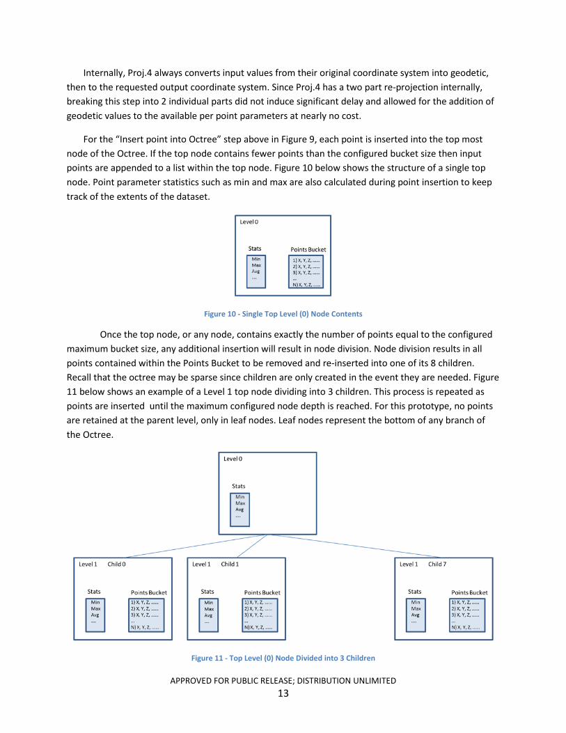
For the “Insert point into Octree” step above in Figure 9, each point is inserted into the top most node of the Octree. If the top node contains fewer points than the configured bucket size then input points are appended to a list within the top node. Figure 10 below shows the structure of a single top node. Point parameter statistics such as min and max are also calculated during point insertion to keep track of the extents of the dataset.

Figure 10 - Single Top Level (0) Node Contents

Once the top node, or any node, contains exactly the number of points equal to the configured maximum bucket size, any additional insertion will result in node division. Node division results in all points contained within the Points Bucket to be removed and re-inserted into one of its 8 children. Recall that the octree may be sparse since children are only created in the event they are needed. Figure 11 below shows an example of a Level 1 top node dividing into 3 children. This process is repeated as points are inserted until the maximum configured node depth is reached. For this prototype, no points are retained at the parent level, only in leaf nodes. Leaf nodes represent the bottom of any branch of the Octree.

Figure 11 - Top Level (0) Node Divided into 3 Children


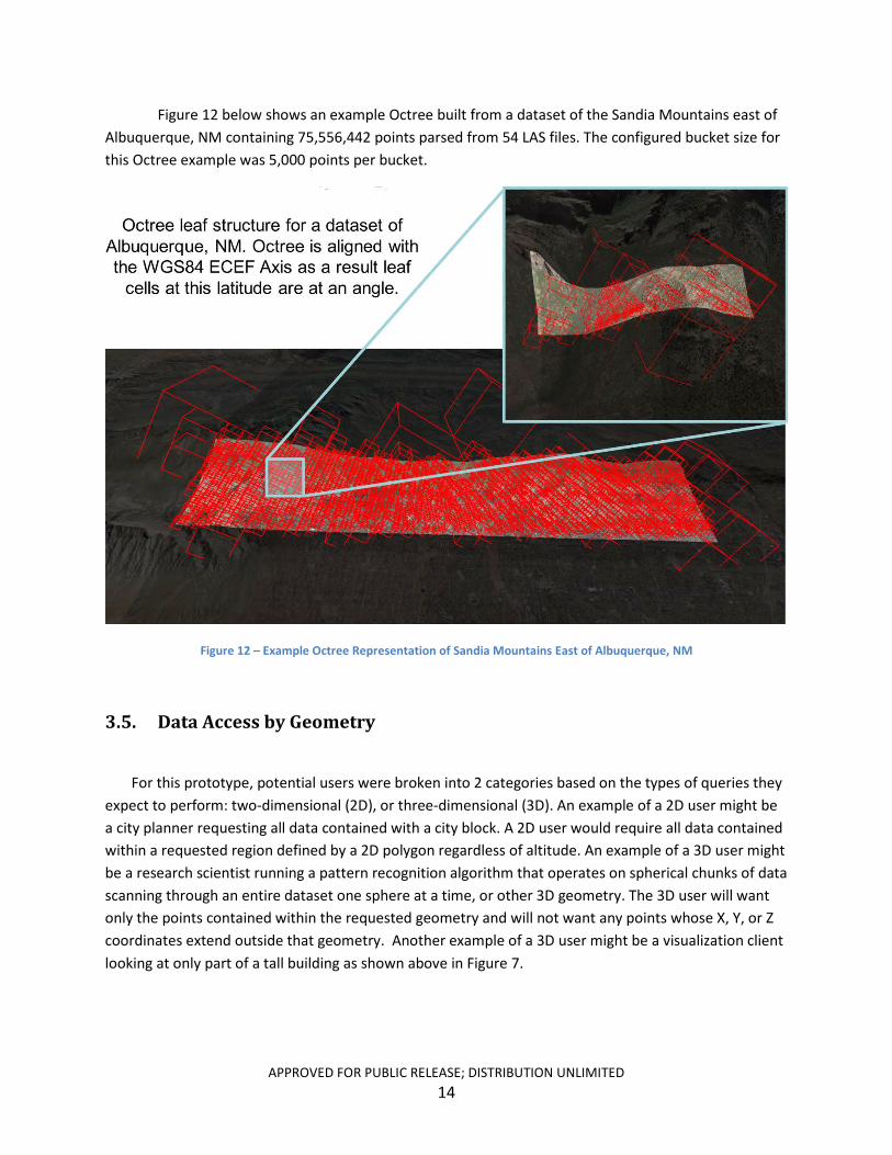
Figure 12 below shows an example Octree built from a dataset of the Sandia Mountains east of Albuquerque, NM containing 75,556,442 points parsed from 54 LAS files. The configured bucket size for this Octree example was 5,000 points per bucket.

Figure 12 – Example Octree Representation of Sandia Mountains East of Albuquerque, NM

3.5. Data Access by Geometry

For this prototype, potential users were broken into 2 categories based on the types of queries they expect to perform: two-dimensional (2D), or three-dimensional (3D). An example of a 2D user might be a city planner requesting all data contained with a city block. A 2D user would require all data contained within a requested region defined by a 2D polygon regardless of altitude. An example of a 3D user might be a research scientist running a pattern recognition algorithm that operates on spherical chunks of data scanning through an entire dataset one sphere at a time, or other 3D geometry. The 3D user will want only the points contained within the requested geometry and will not want any points whose X, Y, or Z coordinates extend outside that geometry. Another example of a 3D user might be a visualization client looking at only part of a tall building as shown above in Figure 7.


3.5.1. 2D Polygon

In order to support access by potential 2D users, a method was added to the Octree data structure that returns all points contained within a simple polygon as defined by a list of vertices in WGS84 geodetic (longitude, latitude) coordinates. As part of the ingestion phase, statistics are calculated during point insertion that include the Octree node (cell) and 2D extents in longitude and latitude. Extents are calculated for both parents and leaf nodes. Treating each node’s 2D extents as a bounding box enables comparison of a requested polygon region to each node through a bounding-box-intersects-polygon test. In reality, a polygon intersects polygon test was implemented since a bounding box is just a very simple polygon. This approach leaves the option later to replace each node’s bounding extent, or bounding box with a hull that more tightly represents the node’s data. Any nodes whose contents are only partially contained within a requested polygon require an additional point in polygon test be performed to prune out any contents that fall outside the requested polygon.

The Computational Geometry Algorithms Library (CGAL) Open Source Project was used for the polygon intersects polygon, and point in polygon tests.

• CGAL – Computational Geometry Algorithms Library http://www.cgal.org/

The polygon intersects polygon test in CGAL returned simply a binary result of true or false, but an ideal test would return a ternary result; 1) does not intersect, 2) partially intersects, 3) completely intersects. Such a ternary test would allow for the ideal example of how to test for polygon intersection shown below in Figure 13. This test would initially be on parents, and would only traverse parents that either partially or completely intersected request polygon.


Figure 13 – Ideal Leaf Node 2D Polygon Intersection Test

Since CGAL did not appear to contain any such ternary version of polygon intersects polygon, the “Fully Contained” branch shown above in Figure 13 was left out of the prototype implementation resulting in a point in polygon being tested on every point within leaf nodes that intersected the request polygon. A “prune” Boolean option was added that if set to false, skips the point in polygon test and simply returns all points as if passing nodes were “Fully Contained”. In many use cases, not pruning these edge points in order to speed up performance may be acceptable. It was possible to determine which nodes were edge nodes for a specific “pruned” request by checking the number of returned points compared to the number of points contained within a point bucket. Figure 14 below shows a triangular request polygon along with its edge nodes (left), and the points which would be returned if those edges are pruned (bottom right), or not pruned (top right).


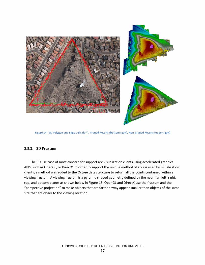
Figure 14 - 2D Polygon and Edge Cells (left), Pruned Results (bottom right), Non-pruned Results (upper right)

3.5.2. 3D Frustum

The 3D use case of most concern for support are visualization clients using accelerated graphics API’s such as OpenGL, or DirectX. In order to support the unique method of access used by visualization clients, a method was added to the Octree data structure to return all the points contained within a viewing frustum. A viewing frustum is a pyramid shaped geometry defined by the near, far, left, right, top, and bottom planes as shown below in Figure 15. OpenGL and DirectX use the frustum and the “perspective projection” to make objects that are farther away appear smaller than objects of the same size that are closer to the viewing location.


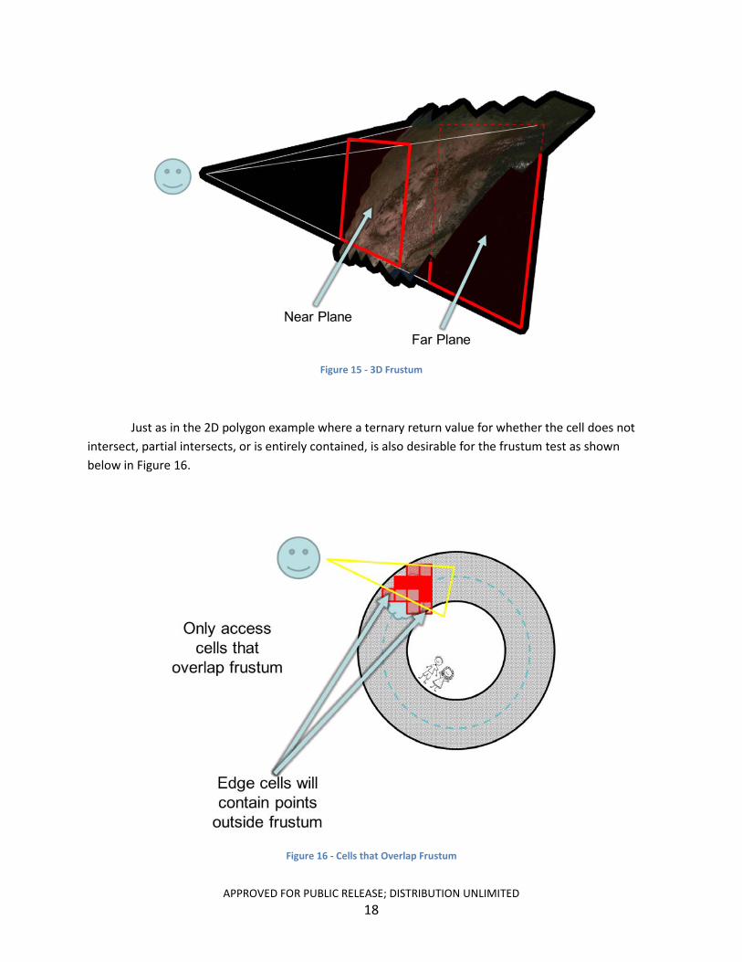
Figure 15 - 3D Frustum

Just as in the 2D polygon example where a ternary return value for whether the cell does not intersect, partial intersects, or is entirely contained, is also desirable for the frustum test as shown below in Figure 16.

Figure 16 - Cells that Overlap Frustum


The ternary intersection test is not only useful for optimizing the pruning of points outside the viewing area, but knowing that a parent is fully contained within the request eliminates the need to further test its children. If a parent is fully contained, then all its children are therefore fully contained as well.

The JView API developed by AFRL is a collection of Java classes that simplify the process of 3D graphics utilizing OpenGL. JView contains a frustum intersects box method that has the desired ternary set of return values. Each node (cell) in the Octree is a perfect box with a closed form solution to calculate the cell resolution as defined above in Table 1. This method from the JView API was ported from JAVA to C++ and implemented in this task’s prototype.

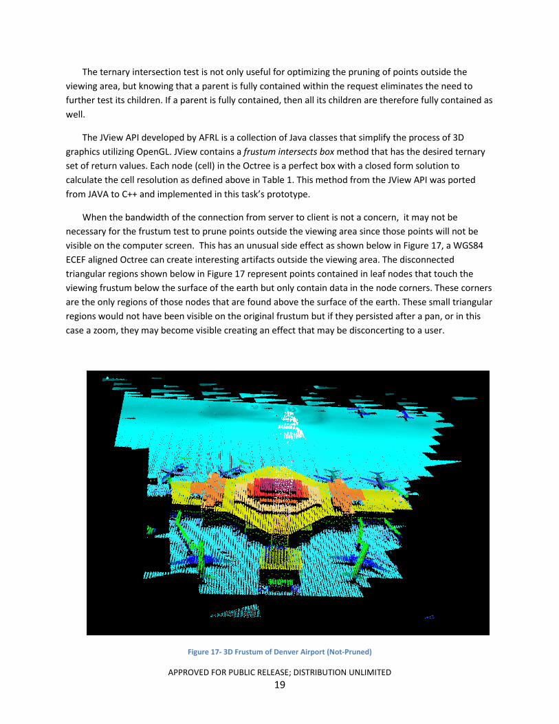
When the bandwidth of the connection from server to client is not a concern, it may not be necessary for the frustum test to prune points outside the viewing area since those points will not be visible on the computer screen. This has an unusual side effect as shown below in Figure 17, a WGS84 ECEF aligned Octree can create interesting artifacts outside the viewing area. The disconnected triangular regions shown below in Figure 17 represent points contained in leaf nodes that touch the viewing frustum below the surface of the earth but only contain data in the node corners. These corners are the only regions of those nodes that are found above the surface of the earth. These small triangular regions would not have been visible on the original frustum but if they persisted after a pan, or in this case a zoom, they may become visible creating an effect that may be disconcerting to a user.

Figure 17- 3D Frustum of Denver Airport (Not-Pruned)


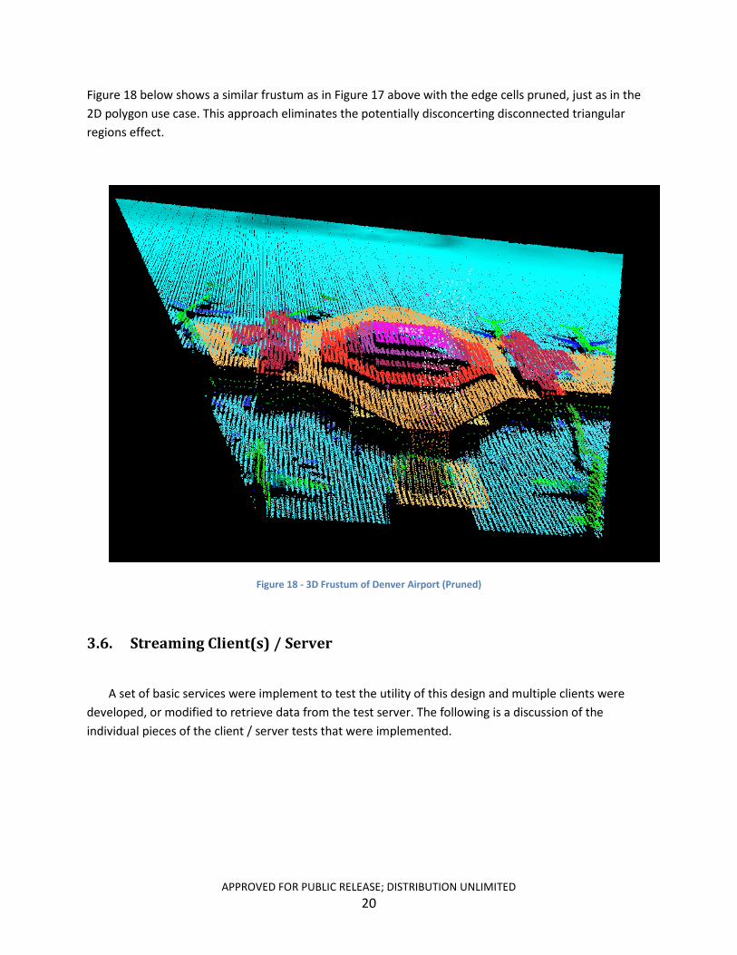
Figure 18 below shows a similar frustum as in Figure 17 above with the edge cells pruned, just as in the 2D polygon use case. This approach eliminates the potentially disconcerting disconnected triangular regions effect.

Figure 18 - 3D Frustum of Denver Airport (Pruned)

3.6. Streaming Client(s) / Server

A set of basic services were implement to test the utility of this design and multiple clients were developed, or modified to retrieve data from the test server. The following is a discussion of the individual pieces of the client / server tests that were implemented.


3.6.1. Easy Socket (C++/JAVA) Messages

The goal of this effort was not to develop, or test communication protocols but rather to research the techniques necessary to rapidly access data based on a 3D partitioning strategy and develop the necessary geometric queries to enable a variety of clients to pull points from a server. Additionally, security was not a concern as this effort would only be run on a trusted network. A simple TCP/IP API in both JAVA, and C++ was developed which creates TCP/IP sockets between a client/host and passes strings, ints, long, and doubles from one machine to another. This API, “EasySocket” was used to develop an initial server, pass client requests, and receive data. The EasySocket API will not be discussed in detail as the only aspect of it relevant to this research is the nature of the messages being passed.

3.6.2. Point Server Prototype

An initial server prototype was developed that accepts configuration settings for bucket size, input data files, input coordinate systems, and port to accept connections on using the following operations;

1. Parse Input Files -> Re-project to ECEF2. Build RAM based Octree (not persisted to disk for this prototype)3. Open TCP/IP port and listen for connections4. Respond to incoming geometric queries, or state changes

The server was put into a state by each client instructing the server as to how many points to transfer per TCP/IP packet, and which parameters (X, Y, Z, Altitude, …) would be included with each point. Modification of the packet size not only impacts performance, but breaking a request up into packets also gives the opportunity to view sub portions of a large request. For example, if a packet size of 5,000 points was selected, and 1,000,000 points would be returned, then a total of 200 packets will be delivered. Table 2 below shows the message options that define state configuration of the prototype server.

Send (String, …) Meaning

SET_PACKETSIZE Int Set Number of Points Send Per Packet

SET_HEADER String 1st Point Parameter Name String 2nd Point Parameter Name …. SET_HEADER_END

Table 2 - Point Cloud Server Configure State Messages


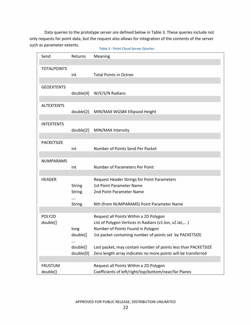
Data queries to the prototype server are defined below in Table 3. These queries include not only requests for point data, but the request also allows for integration of the contents of the server such as parameter extents.

Send Returns Meaning

TOTALPOINTS int Total Points in Octree

GEOEXTENTS double[4] W/E/S/N Radians

ALTEXTENTS double[2] MIN/MAX WGS84 Ellipsoid Height

INTEXTENTS double[2] MIN/MAX Intensity

PACKETSIZE int Number of Points Send Per Packet

NUMPARAMS int Number of Parameters Per Point

HEADER Request Header Strings for Point Parameters String 1st Point Parameter Name String 2nd Point Parameter Name …. String Nth (from NUMPARAMS) Point Parameter Name

POLY2D Request all Points Within a 2D Polygon double[] List of Polygon Vertices in Radians (v1.lon, v2.lat,… )

long Number of Points Found in Polygon double[] 1st packet containing number of points set by PACKETSIZE …. double[] Last packet, may contain number of points less than PACKETSIZE double[0] Zero length array indicates no more points will be transferred

FRUSTUM Request all Points Within a 2D Polygon double[] Coefficients of left/right/top/bottom/near/far Planes

Table 3 - Point Cloud Server Queries


3.6.3. JView World Client

Multiple clients were either modified, or developed, to simulate potential use cases of the server. JView World is a component of AFRL’s JView API that adds a 3D globe with elevation data and imagery to any Java application. JView also includes a generic point rendering object that is suitable to drawing points in the scene up to several millions points. JView by default does not include a Level of Detail (LOD) for its point rendering, ultimately limiting its scalability. A test application was created that allows a user to pan and zoom to a specific location and manually trigger a query to the server requesting all data within the current viewing frustum. JView World can provide the user the current coefficients needed to define the 6 mathematical planes representing the bounds of the frustums near, far, right, left, top and bottom. Figure 17 and Figure 18 above show the results of a frustum based query made through JView World. In Figure 17 and Figure 18 the underlying 3D globe is not drawn allowing for a unobstructed view of the point data.

JView World includes an extendable ability to page various data sources in and out of the viewing frustum based on what is currently visible in the scene using 2D bounding regions defined by longitude and latitude. Utilizing this 2D capability, a second test was developed that performs 2D polygon based queries. This approach also allows for basic panning and zooming. Figure 19 below shows the results of using JView to draw DARPA’s URGENT datasets for a portion of the city of Ottawa, Canada.

Figure 19 - JView World with DARPA URGENT Point Cloud Data for a Sub Region of Ottawa, Canada


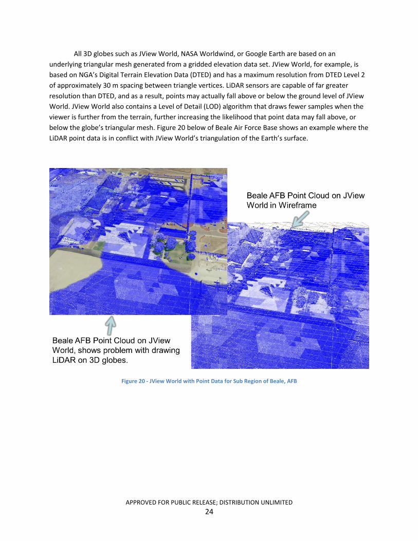
All 3D globes such as JView World, NASA Worldwind, or Google Earth are based on an underlying triangular mesh generated from a gridded elevation data set. JView World, for example, is based on NGA’s Digital Terrain Elevation Data (DTED) and has a maximum resolution from DTED Level 2 of approximately 30 m spacing between triangle vertices. LiDAR sensors are capable of far greater resolution than DTED, and as a result, points may actually fall above or below the ground level of JView World. JView World also contains a Level of Detail (LOD) algorithm that draws fewer samples when the viewer is further from the terrain, further increasing the likelihood that point data may fall above, or below the globe’s triangular mesh. Figure 20 below of Beale Air Force Base shows an example where the LiDAR point data is in conflict with JView World’s triangulation of the Earth’s surface.

Figure 20 - JView World with Point Data for Sub Region of Beale, AFB


3.6.4. JDAR Client

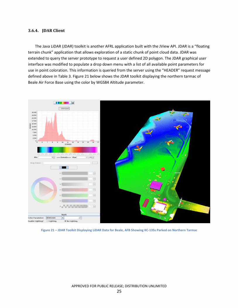
The Java LiDAR (JDAR) toolkit is another AFRL application built with the JView API. JDAR is a “floating terrain chunk” application that allows exploration of a static chunk of point cloud data. JDAR was extended to query the server prototype to request a user defined 2D polygon. The JDAR graphical user interface was modified to populate a drop down menu with a list of all available point parameters for use in point coloration. This information is queried from the server using the “HEADER” request message defined above in Table 3. Figure 21 below shows the JDAR toolkit displaying the northern tarmac of Beale Air Force Base using the color by WGS84 Altitude parameter.

Figure 21 – JDAR Toolkit Displaying LiDAR Data for Beale, AFB Showing KC-135s Parked on Northern Tarmac


3.6.5. WebGL Client (VISRIDER Task #6)

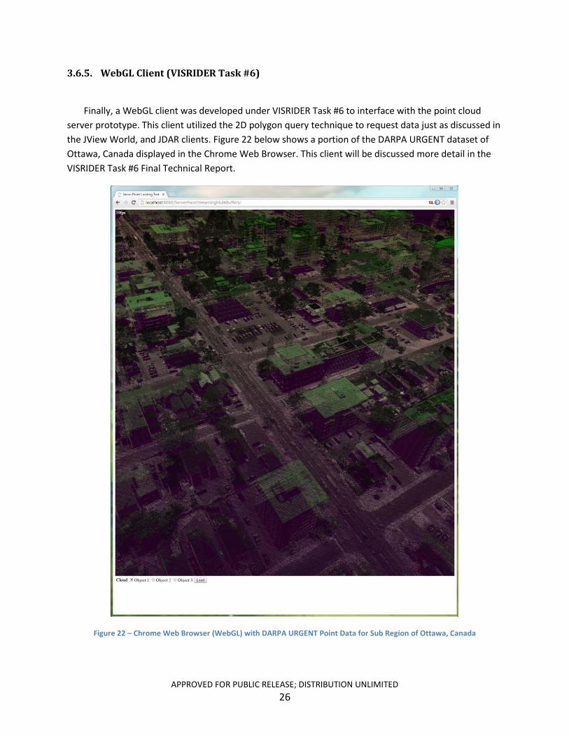
Finally, a WebGL client was developed under VISRIDER Task #6 to interface with the point cloud server prototype. This client utilized the 2D polygon query technique to request data just as discussed in the JView World, and JDAR clients. Figure 22 below shows a portion of the DARPA URGENT dataset of Ottawa, Canada displayed in the Chrome Web Browser. This client will be discussed more detail in the VISRIDER Task #6 Final Technical Report.

Figure 22 – Chrome Web Browser (WebGL) with DARPA URGENT Point Data for Sub Region of Ottawa, Canada


3.7. Performance Characteristics

For data contained within this section performance characteristics were generated using 2 identical systems with the following specifications.

OS Debian GNU/Linux 7.6 (wheezy) CPU GPU

Duel Intel ® Xeon® Eight-Core E5-2650 @ 2.0 GHz NVidia K5000

RAM 128 GB HD Speed 7200 RPM SATA

Development Language C++ / gcc (Debian 4.7.2-5) 4.7.2

Table 4 - Performance Test(s) System Configuration

3.7.1. Ingestion

Multiple datasets were ingested as part of the performance testing phase of this effort. Results are presented for a specific dataset downloaded from the UGSG Earth Explorer Website for Albuquerque, NM collected in 2010. Table 5 shows the ingestion performance statics for this dataset.

LAS File Count 54 Size on Disk

Coordinate System / Datum(s) Number of Points

Maximum Bucket Size Total Time for all Operations

6 G UTM Zone 13 NAD83 / NAVD88 75,556,442 pts 1000 pts 69.651 s

Time to parse all files 5.88 s (8.44% of total time) Time to re-project into ECEF

Time to Insert into Octree Avg Time for all Operations per Point

43.542 s (62.51% of total time) 20.229 s (29.04% of total time) .0009218 ms

Size of Octree In RAM 7.7 G

Table 5 – Summary of Ingestion Performance Statistics

Using the per point parse and re-project time from Table 5 and assuming that performance would be constant Table 6 below shows and estimate of the amount of time it would take to ingest 1 Trillion Points.

Parse Time Re-project

Insert into Octree Time

.9 days 6.67 days 3.1 days

Total Time for all Operations 10.67 days

Table 6 - Estimated Time to Ingest 1 Trillion Points


3.7.2. Access

3.7.2.1. 2D Polygon

C++ and Java unit tests were implemented that query for data bounded by the triangular polygon shown above in Figure 14 from the test dataset. These unit tests were executed for both the not-pruned example shown in the upper right of Figure 14, and the pruned shown in the bottom right. The performance of the client and server for the C++ unit test for the “not-pruned” polygon are shown below in Table 7, and the results of the “pruned” polygon test is shown in Table 8.

Points Identified Per Point Parameters

262,104 pts 7 doubles

Server Packet Size 5,000 pts / packets = 35,000 doubles / packet

Time to identify points .436 s Time to serve points 1.182 s

Time to receive points 1.817 s

Table 7 - 2D Polygon Query Client/Server Performance Statistics (Not-Pruned)






Table 8 - 2D Polygon Query Client/Server Performance Statistics (Pruned)

Table 7 and Table 8 show the results of an individual execution of each test, and do not represent an average over a series of runs. Further testing still needs to be performed on a stand-alone network averaging multiple runs with diverse sets of data. The client and server were networked over a Gigabit network with a varying about of traffic causing inconsistent results for transfer rates, but the time to identify points remained relatively constant over multiple runs. Identification of points within the data structure took almost twice as long in the pruned polygon request as it did in the non-pruned test. The reason for the increased point identification time in the pruned request is the requirement to


perform a point in polygon test on all points within Octree cells that partially intersect the request polygon.

3.7.2.2. 3D Frustum

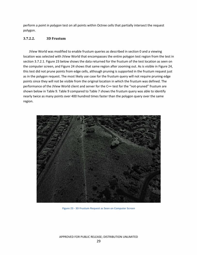
JView World was modified to enable frustum queries as described in section 0 and a viewing location was selected with JView World that encompasses the entire polygon test region from the test in section 3.7.2.1. Figure 23 below shows the data returned for the frustum of the test location as seen on the computer screen, and Figure 24 shows that same region after zooming out. As is visible in Figure 24, this test did not prune points from edge cells, although pruning is supported in the frustum request just as in the polygon request. The most likely use case for the frustum query will not require pruning edge points since they will not be visible from the original location in which the frustum was defined. The performance of the JView World client and server for the C++ test for the “not-pruned” frustum are shown below in Table 9. Table 9 compared to Table 7 shows the frustum query was able to identify nearly twice as many points over 400 hundred times faster than the polygon query over the same region.

Figure 23 - 3D Frustum Request as Seen on Computer Screen


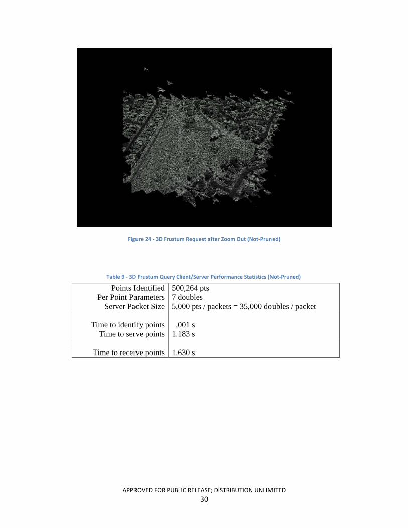
Figure 24 - 3D Frustum Request after Zoom Out (Not-Pruned)






Table 9 - 3D Frustum Query Client/Server Performance Statistics (Not-Pruned)


4.0 Results and Discussion

The prototype developed for this effort utilized a globally defined Octree data structure utilizing the WGS84 Earth Centered Earth Fixed (ECEF) Coordinate System. As shown above in Figure 5 re-projection of data distributed in projected coordinate systems, such as the State Plane Coordinate System (SPC) or Universal Transverse Mercator (UTM), into ECEF during data ingestion often takes twice as long as parsing the data from disk and building the Octree. Due to the amount of time required for re-projection, this operation represents the largest bottleneck for processing this data during ingest. This prototype preformed all the re-projections utilizing a single core (thread) but signification performance improvement could easily be achieve through parallelization of this portion of the process. An even better approach would be to stop distributing these datasets in projected coordinate systems in the first place. LiDAR collection platforms geo-locate these datasets based on GPS coordinates that are based on ECEF. There is no compelling reason to convert the datasets into projected coordinates for distribution other than keeping with the legacy of the GIS community being most comfortable in SPC and UTM.

The performance test of a 3D frustum query versus 2D polygon was able to identify nearly twice as many points over 400 hundred times faster than the polygon query over a similar region. There are two reasons for this; the first being the mathematical operations for testing intersection of a cube within a frustum is much simpler than polygon intersects polygon; the second reason is the frustum test ported from JView contained a ternary condition indicating that the cube either: did not intersect, partially intersected, or is entirely contained within the frustum. The 3rd condition, entirely contained within frustum, provides an optimization for the frustum test that allows all tests to be skipped on children of parents that are entirely contained within a frustum. CGAL’s polygon intersects polygon test was used for the 2D case and contained only the standard Boolean, does or does not, intersect. Future versions of this approach should incorporate a ternary condition for polygon intersects polygon, enabling the algorithmic approach shown above in Figure 13. This optimization would even further increase performance in the case of pruned polygons as it would completely eliminate the need to perform a point in polygon test on nodes that are completely contained within the polygon. It is believed that with this optimization the polygon query performance would be more comparable to the frustum query performance.

This effort focused on data structure performance characteristics and streaming techniques but did not explore the Level of Detail (LOD) possibilities that using an Octree for spatial acceleration could enable. An obvious option would be to leave a subset of the data at each level of the tree that could be provided as a lower level representation, and then increase the data density as requested by streaming in children until the bottom of the tree is reached. Additional research is necessary to determine what data should be left behind in parent nodes to achieve desirable LOD effects. Common approaches include simply skipping, or randomly selecting points for level of detail, but other efforts have shown these approaches have varying results which depend heavily on the dataset characteristics.


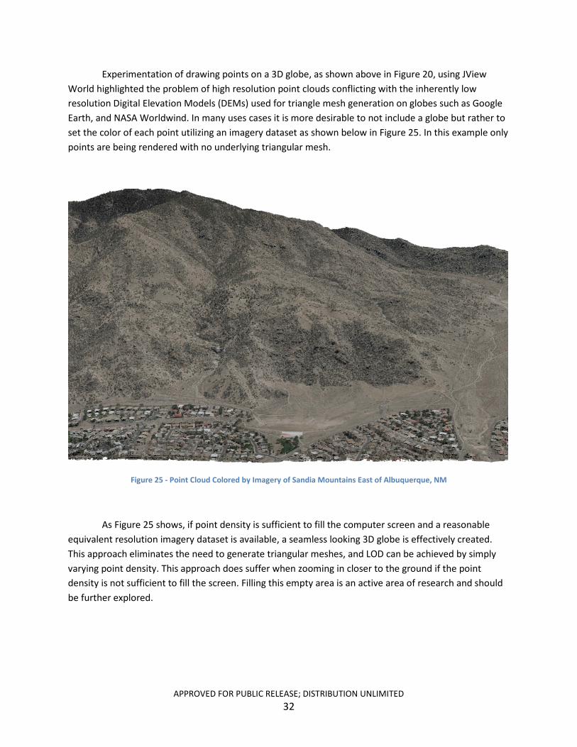
Experimentation of drawing points on a 3D globe, as shown above in Figure 20, using JView World highlighted the problem of high resolution point clouds conflicting with the inherently low resolution Digital Elevation Models (DEMs) used for triangle mesh generation on globes such as Google Earth, and NASA Worldwind. In many uses cases it is more desirable to not include a globe but rather to set the color of each point utilizing an imagery dataset as shown below in Figure 25. In this example only points are being rendered with no underlying triangular mesh.

Figure 25 - Point Cloud Colored by Imagery of Sandia Mountains East of Albuquerque, NM

As Figure 25 shows, if point density is sufficient to fill the computer screen and a reasonable equivalent resolution imagery dataset is available, a seamless looking 3D globe is effectively created. This approach eliminates the need to generate triangular meshes, and LOD can be achieved by simply varying point density. This approach does suffer when zooming in closer to the ground if the point density is not sufficient to fill the screen. Filling this empty area is an active area of research and should be further explored.


5.0 Conclusions

The primary focus of this effort was the design and implementation of a prototype data structure for 3D spatial acceleration that can be dynamically modified and accessed on a global scale. The prototype developed for this effort utilized a globally defined Octree data structure utilizing the WGS84 Earth Centered Earth Fixed (ECEF) Coordinate System. Integration of this prototype with existing applications such as JView World, and JDAR demonstrated this design approach was an efficient, contiguous, and global approach to handling massive point clouds.

Usage of a projected coordinate system for data that is 3D in its nature, such as LiDAR, is not practical and is an artifact of the way the GIS community still thinks in terms of 2D maps where the majority of products are imagery. The ideal coordinate system for computer software processing LiDAR data is the Earth Centered Cartesian coordinate system defined by the World Geodetic System of 1984 (WGS84). This effort demonstrated the usage of point clouds in the ECEF coordinate system along with examples and performance metrics of how to:1) access data with traditional 2D polygon based queries, and 2)apply 3D frustum based queries suitable for use with modern 3D graphics API’s such as OpenGL.

Future research that builds on this effort should include: 1) Advanced Level of Detail (LOD) approaches that calculate how to create lower resolution subsets of data at parent levels, 2) Various methods of persisting the Octree on disk and 3) additional techniques that parallelize the operations used during data ingestion.


6.0 References

Applied Imagery. (2013). Quick Terrain Modeler. Retrieved Dec 2, 2013, from http://appliedimagery.com/

ASPRS. (2013, July 15). LAS Specification. Retrieved Aug 30, 2013, from http://www.asprs.org/a/society/committees/standards/LAS_1_4_r13.pdf

Moore, J., & McVay, A. (2008, Jul). Out-of-Core Digital Terrain Elevation Data (DTED) Visualization. Retrieved Oct 30, 2013, from DTIC Online: http://www.dtic.mil/dtic/

NGA. (2013, Apr). nga (U) Universal Transverse Mercator (UTM) (UNCLASSIFIED). Retrieved Aug 30, 2013, from http://earth-info.nga.mil/GandG/coordsys/grids/utm.html

NOAA. (2007). Datums, Heights and Geodesy. Retrieved Aug 30, 2013, from http://www.ngs.noaa.gov/GEOID/PRESENTATIONS/2007_02_24_CCPS/Roman_A_PLSC2007notes.pdf

(1990). In H. Samet, The Design and Analysis of Spatial Data Structures. Boston, MA, USA: Addison-Wesley Longman Publishing Co., Inc.

(1990). In H. Samet, Applications of Spatial Data Structures: Computer Graphics, Image Processing, and GIS. Reading, MA, USA: Addison-Wesley.

USGS. (n.d.). Earth Explorer. Retrieved from http://earthexplorer.usgs.gov/


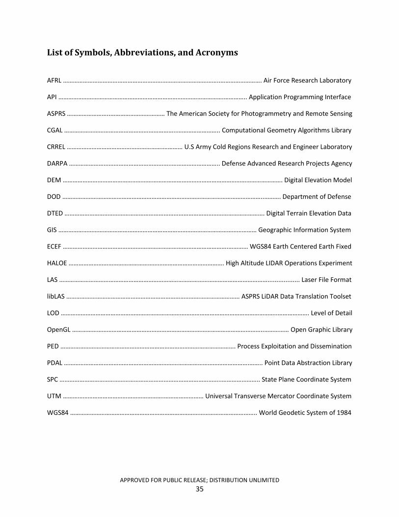
List of Symbols, Abbreviations, and Acronyms

AFRL …………………………………………………………………………………..……………………. Air Force Research Laboratory

API ……………………………………………………………………………………….………….. Application Programming Interface

ASPRS ……………………..…………………………… The American Society for Photogrammetry and Remote Sensing

CGAL …………………………………………………………..…………………….. Computational Geometry Algorithms Library

CRREL ………………………………………………….………… U.S Army Cold Regions Research and Engineer Laboratory

DARPA ……………………………………………………..……………………….. Defense Advanced Research Projects Agency

DEM ……………………………………………………………………………………………………………………. Digital Elevation Model

DOD …………………………………………………………………………………………………………..………. Department of Defense

DTED …………………………………………………………………………………………………………. Digital Terrain Elevation Data

GIS ………………………………………………………………………………………………………… Geographic Information System

ECEF ……………………………………………………………………………………….………… WGS84 Earth Centered Earth Fixed

HALOE …………………………………………………………………………………. High Altitude LIDAR Operations Experiment

LAS ……………………………………………………………………………………………………………….................. Laser File Format

libLAS …………………………………………………………………………………………… ASPRS LiDAR Data Translation Toolset

LOD …………………………………………………………………………………………………………………..………………. Level of Detail

OpenGL ……………………………………………………………………………………………………..…………… Open Graphic Library

PED ……………………………………………………………………………………………. Process Exploitation and Dissemination

PDAL ………………………………………………………………………………………………….…….. Point Data Abstraction Library

SPC ……………………………………………………………………………………..………………….. State Plane Coordinate System

UTM …………………………………………………….…………………… Universal Transverse Mercator Coordinate System

WGS84 ………………………………………………………………………………………………….. World Geodetic System of 1984


Documents

POINT CLOUD STORAGE AND ACCESS ON A GLOBAL SCALE - DTIC