Embed Size (px)
Citation preview
Point-to-Point Shortest Path Algorithms
with Preprocessing
Andrew V. Goldberg
Microsoft Research – Silicon Valley
www.research.microsoft.com/∼goldberg/
Joint work with
Chris Harrelson, Haim Kaplan, and Retato Werneck

Einstein Quote
Everything should be made as simple as possible, but not simpler
SOFSEM 07 1
Shortest Path Problem
Variants
• Non-negative and arbitrary arc lengths.
• Point to point, single source, all pairs.
• Directed and undirected.
Here we study
• Point to point, non-negative length, directed problem.
• Allow preprocessing with limited (linear) space.
Many applications, both directly and as a subroutine.
SOFSEM 07 2
Shortest Path Problem
Input: Directed graph G = (V, A), non-negative length function
ℓ : A → R+, source s ∈ V , terminal t ∈ V .
Preprocessing: Limited space to store results.
Query: Find a shortest path from s to t.
Interested in exact algorithms that search a subgraph.
Related work: reach-based routing [Gutman 04], hierarchi-
cal decomposition [Schultz, Wagner & Weihe 02], [Sanders &
Schultes 05, 06], geometric pruning [Wagner & Willhalm 03], arc
flags [Lauther 04], [Kohler, Mohring & Schilling 05], [Mohring
et al. 06].
SOFSEM 07 3
Motivating Application
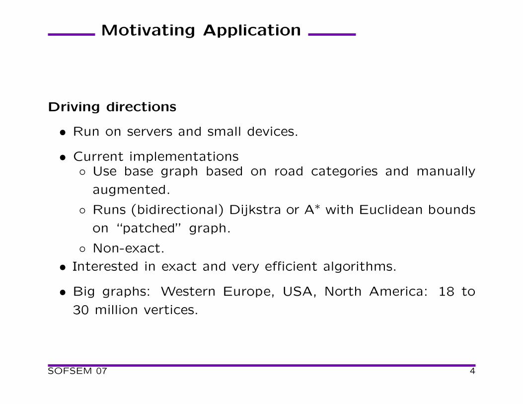
Driving directions
• Run on servers and small devices.
• Current implementations◦ Use base graph based on road categories and manually
augmented.
◦ Runs (bidirectional) Dijkstra or A∗ with Euclidean bounds
on “patched” graph.
◦ Non-exact.
• Interested in exact and very efficient algorithms.
• Big graphs: Western Europe, USA, North America: 18 to
30 million vertices.
SOFSEM 07 4
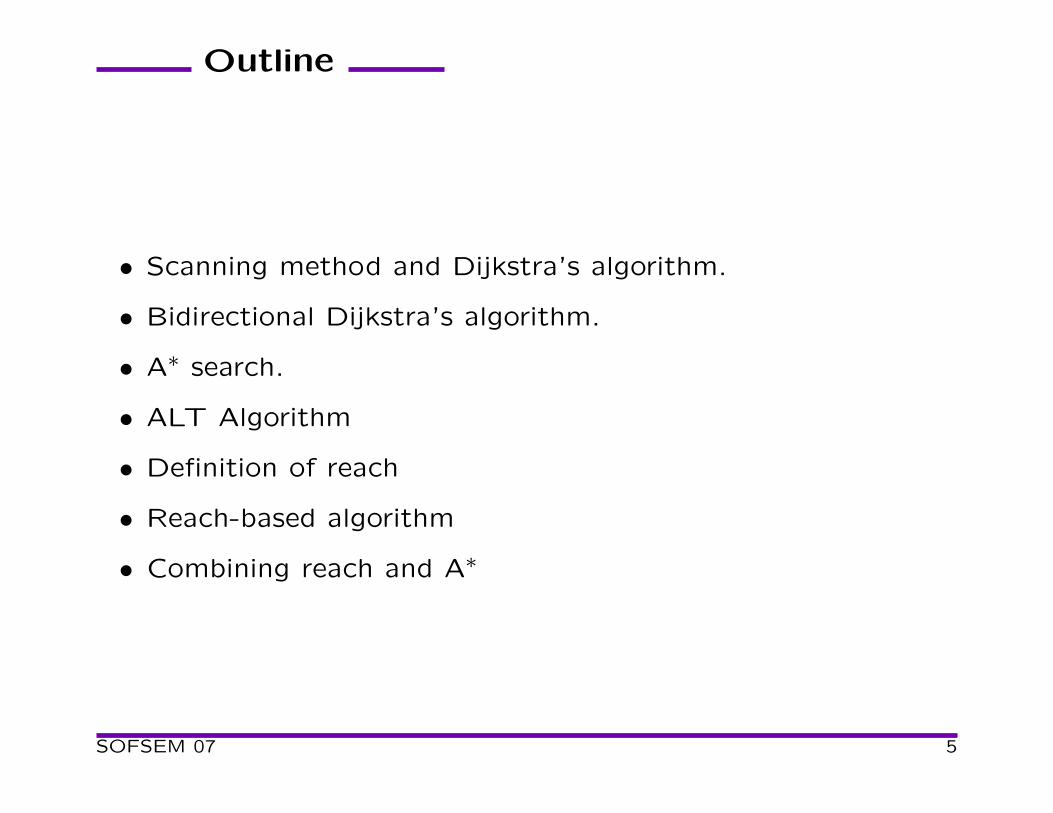
Outline
• Scanning method and Dijkstra’s algorithm.
• Bidirectional Dijkstra’s algorithm.
• A∗ search.
• ALT Algorithm
• Definition of reach
• Reach-based algorithm
• Combining reach and A∗
SOFSEM 07 5
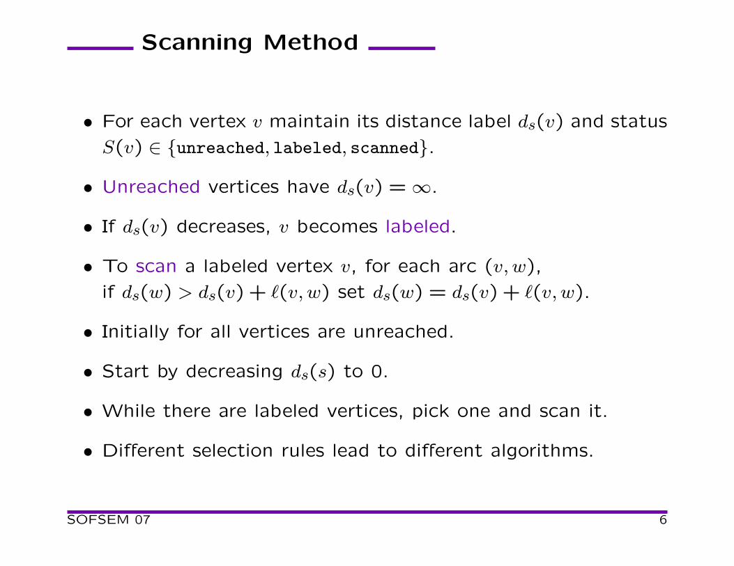
Scanning Method
• For each vertex v maintain its distance label ds(v) and status
S(v) ∈ {unreached, labeled, scanned}.
• Unreached vertices have ds(v) = ∞.
• If ds(v) decreases, v becomes labeled.
• To scan a labeled vertex v, for each arc (v, w),
if ds(w) > ds(v) + ℓ(v, w) set ds(w) = ds(v) + ℓ(v, w).
• Initially for all vertices are unreached.
• Start by decreasing ds(s) to 0.
• While there are labeled vertices, pick one and scan it.
• Different selection rules lead to different algorithms.
SOFSEM 07 6
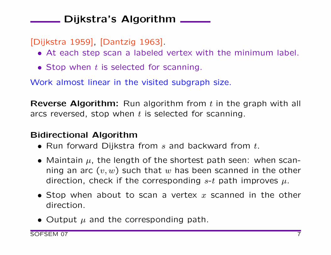
Dijkstra’s Algorithm
[Dijkstra 1959], [Dantzig 1963].
• At each step scan a labeled vertex with the minimum label.
• Stop when t is selected for scanning.
Work almost linear in the visited subgraph size.
Reverse Algorithm: Run algorithm from t in the graph with all
arcs reversed, stop when t is selected for scanning.
Bidirectional Algorithm
• Run forward Dijkstra from s and backward from t.
• Maintain µ, the length of the shortest path seen: when scan-
ning an arc (v, w) such that w has been scanned in the other
direction, check if the corresponding s-t path improves µ.
• Stop when about to scan a vertex x scanned in the other
direction.
• Output µ and the corresponding path.
SOFSEM 07 7
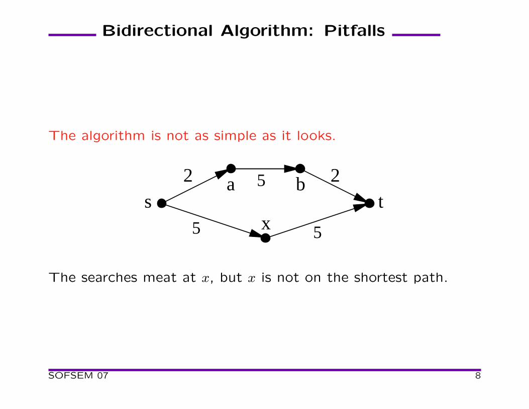
Bidirectional Algorithm: Pitfalls
The algorithm is not as simple as it looks.
5x
2 2s t
ba 5
5
The searches meat at x, but x is not on the shortest path.
SOFSEM 07 8
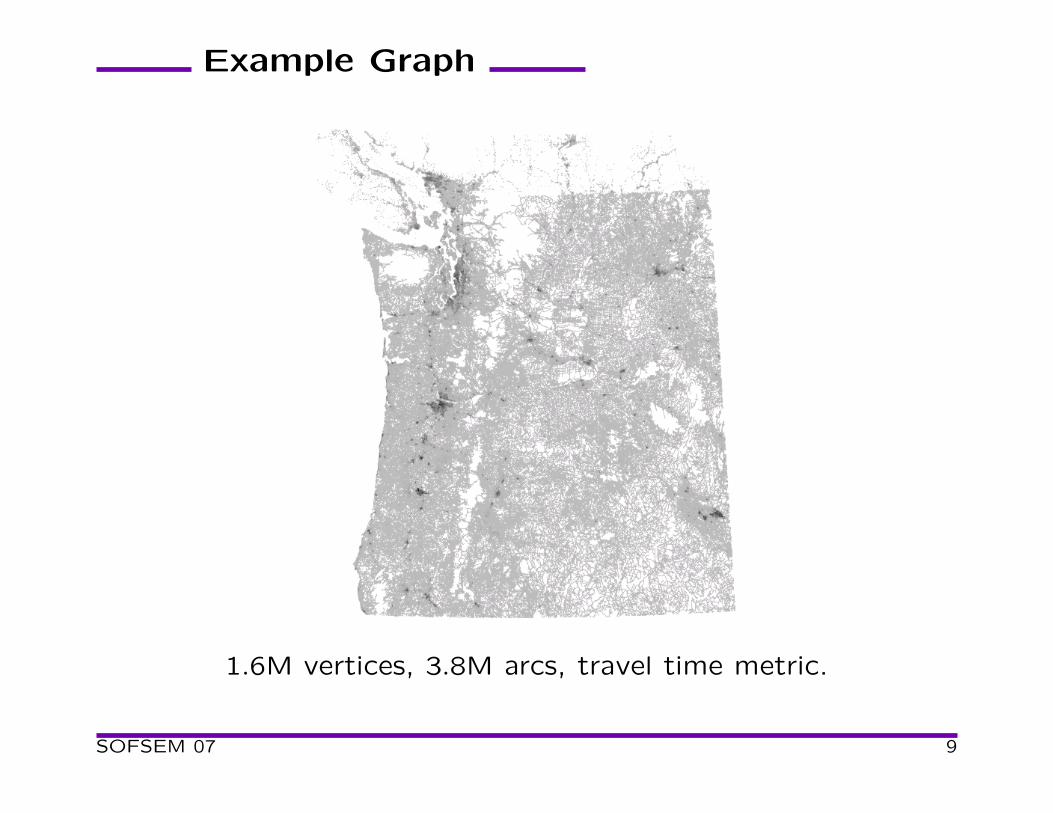
Example Graph
1.6M vertices, 3.8M arcs, travel time metric.
SOFSEM 07 9
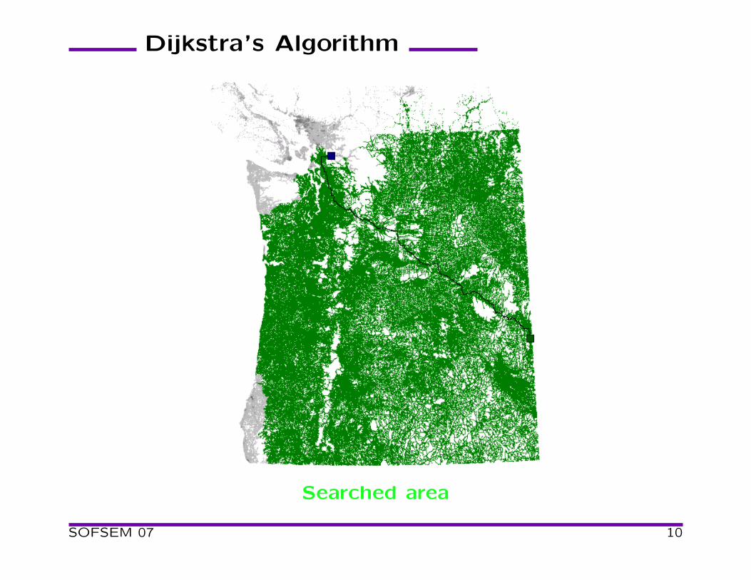
Dijkstra’s Algorithm
Searched area
SOFSEM 07 10
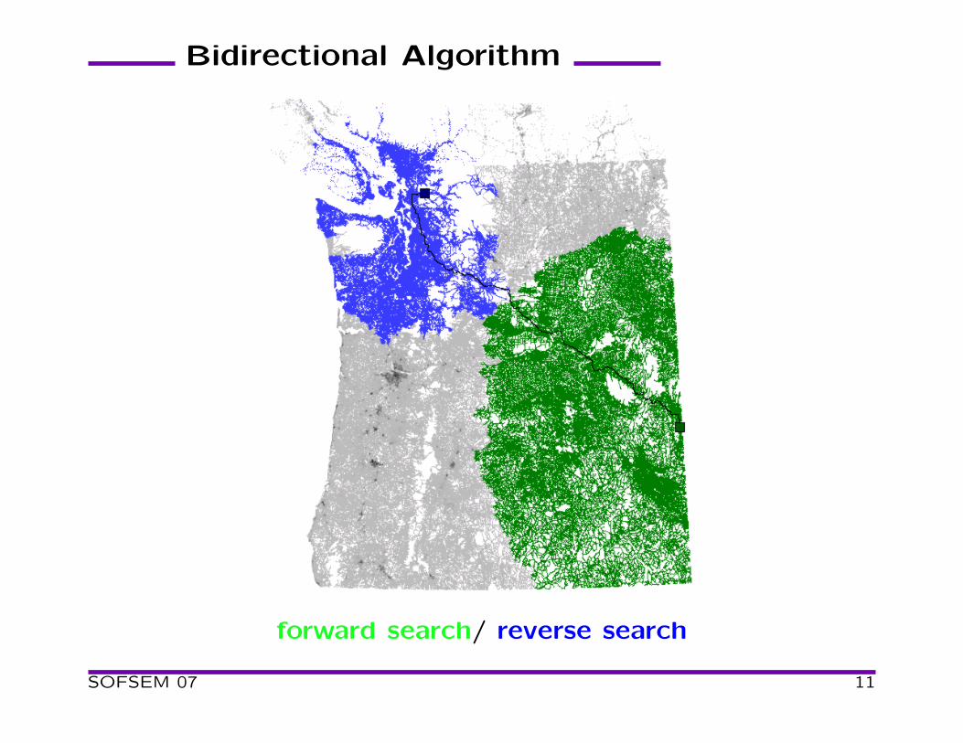
Bidirectional Algorithm
forward search/ reverse search
SOFSEM 07 11
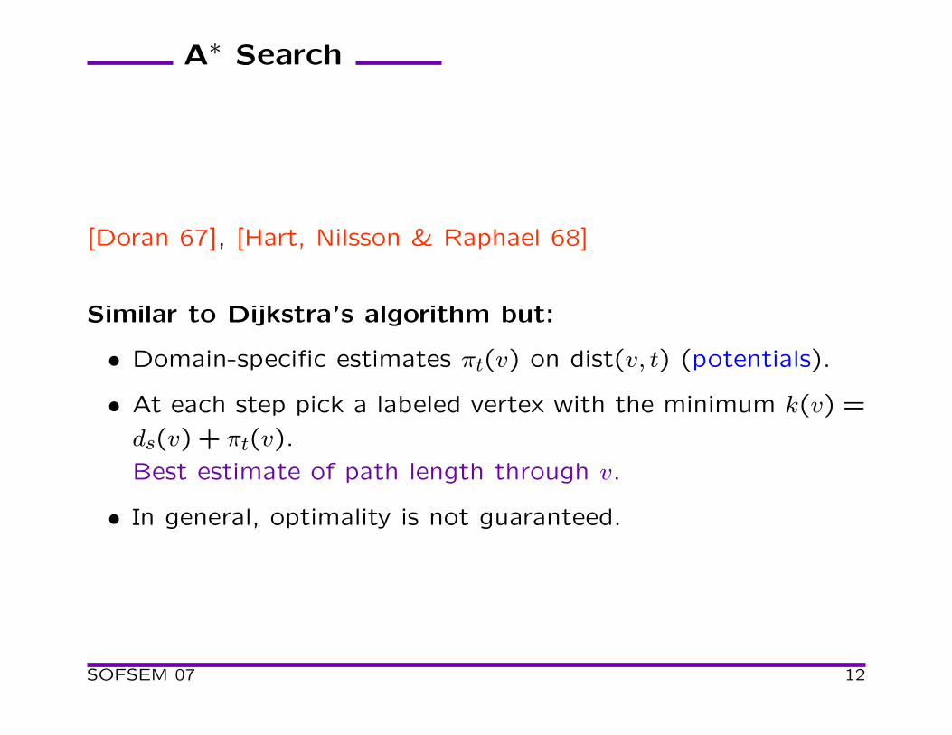
A∗ Search
[Doran 67], [Hart, Nilsson & Raphael 68]
Similar to Dijkstra’s algorithm but:
• Domain-specific estimates πt(v) on dist(v, t) (potentials).
• At each step pick a labeled vertex with the minimum k(v) =
ds(v) + πt(v).
Best estimate of path length through v.
• In general, optimality is not guaranteed.
SOFSEM 07 12
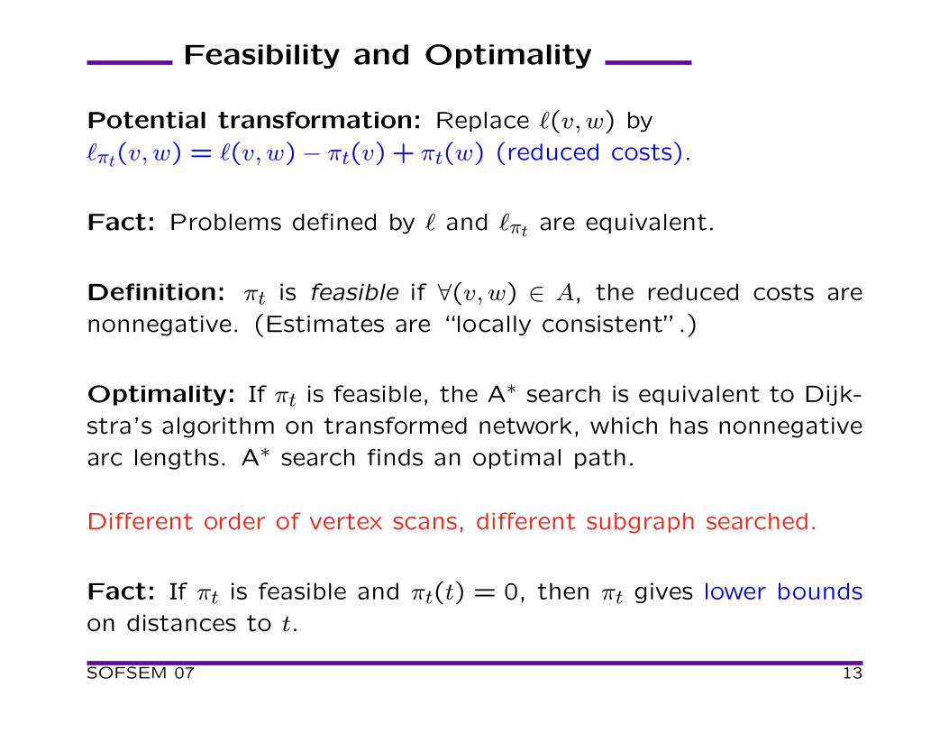
Feasibility and Optimality
Potential transformation: Replace ℓ(v, w) by
ℓπt(v, w) = ℓ(v, w) − πt(v) + πt(w) (reduced costs).
Fact: Problems defined by ℓ and ℓπt are equivalent.
Definition: πt is feasible if ∀(v, w) ∈ A, the reduced costs are
nonnegative. (Estimates are “locally consistent”.)
Optimality: If πt is feasible, the A∗ search is equivalent to Dijk-
stra’s algorithm on transformed network, which has nonnegative
arc lengths. A∗ search finds an optimal path.
Different order of vertex scans, different subgraph searched.
Fact: If πt is feasible and πt(t) = 0, then πt gives lower bounds
on distances to t.
SOFSEM 07 13
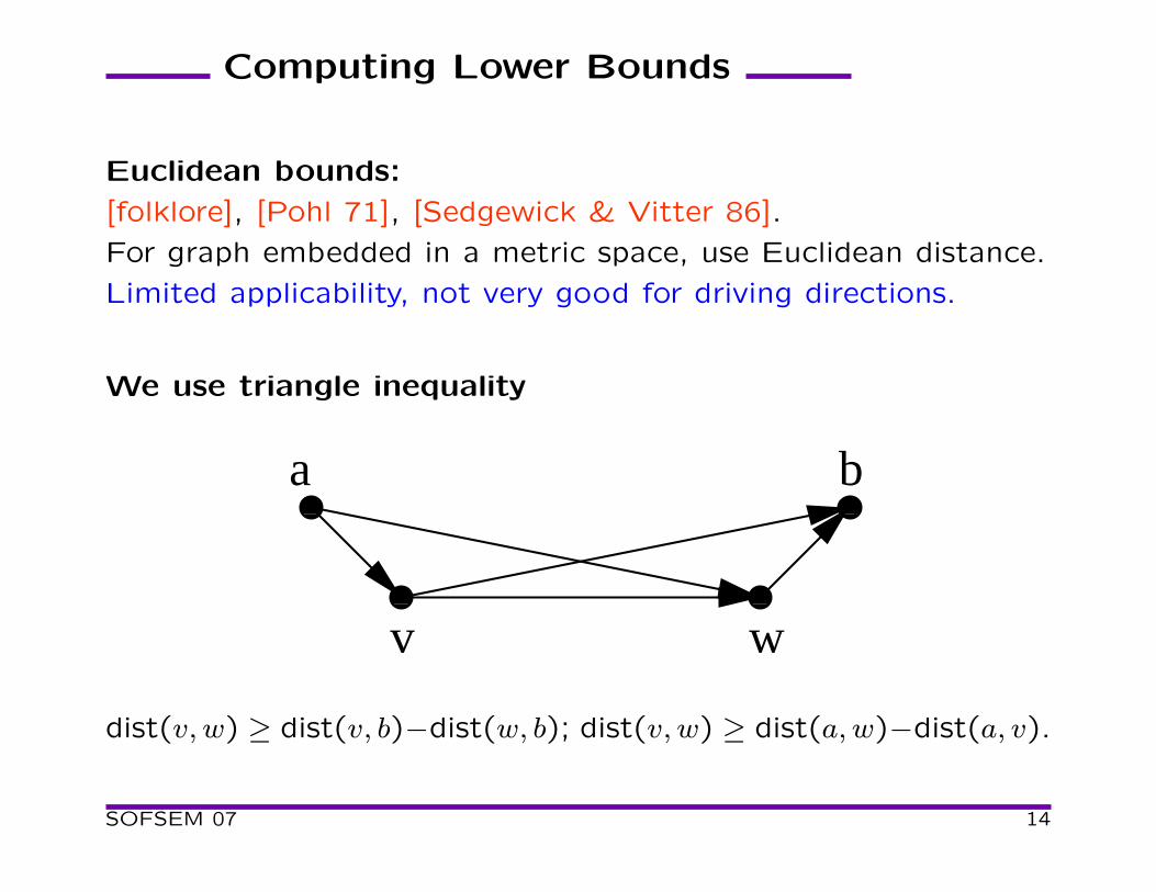
Computing Lower Bounds
Euclidean bounds:
[folklore], [Pohl 71], [Sedgewick & Vitter 86].
For graph embedded in a metric space, use Euclidean distance.
Limited applicability, not very good for driving directions.
We use triangle inequality
����
����
����
����
������������������
������������������
������������������������������������������������������������������������������
������������������������������������������������������������������������������
������������������
������������������
������������������������������������������������������������������������������
������������������������������������������������������������������������������
v w
a b
dist(v, w) ≥ dist(v, b)−dist(w, b); dist(v, w) ≥ dist(a, w)−dist(a, v).
SOFSEM 07 14
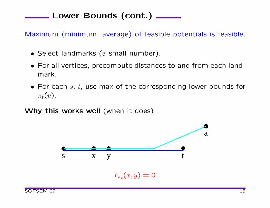
Lower Bounds (cont.)
Maximum (minimum, average) of feasible potentials is feasible.
• Select landmarks (a small number).
• For all vertices, precompute distances to and from each land-
mark.
• For each s, t, use max of the corresponding lower bounds for
πt(v).
Why this works well (when it does)
s t
a
x y
ℓπt(x, y) = 0
SOFSEM 07 15
Bidirectional Lower-bounding
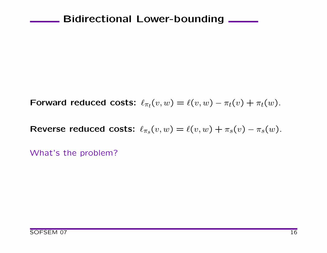
Forward reduced costs: ℓπt(v, w) = ℓ(v, w) − πt(v) + πt(w).
Reverse reduced costs: ℓπs(v, w) = ℓ(v, w) + πs(v) − πs(w).
What’s the problem?
SOFSEM 07 16
Bidirectional Lower-bounding
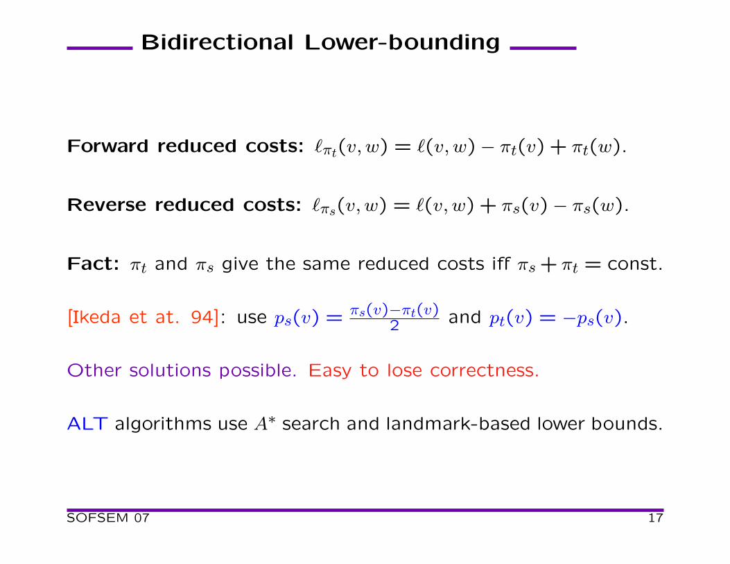
Forward reduced costs: ℓπt(v, w) = ℓ(v, w) − πt(v) + πt(w).
Reverse reduced costs: ℓπs(v, w) = ℓ(v, w) + πs(v) − πs(w).
Fact: πt and πs give the same reduced costs iff πs + πt = const.
[Ikeda et at. 94]: use ps(v) = πs(v)−πt(v)2 and pt(v) = −ps(v).
Other solutions possible. Easy to lose correctness.
ALT algorithms use A∗ search and landmark-based lower bounds.
SOFSEM 07 17
Landmark Selection
Preprocessing
• Random selection is fast.
• Many heuristics find better landmarks.
• Local search can find a good subset of candidate landmarks.
• We use a heuristic with local search.
Preprocessing/query trade-off.
Query
• For a specific s, t pair, only some landmarks are useful.
• Use only active landmarks that give best bounds on dist(s, t).
• If needed, dynamically add active landmarks (good for the
search frontier).
• Only three active landmarks on the average.
Allows using many landmarks with small time overhead.
SOFSEM 07 18
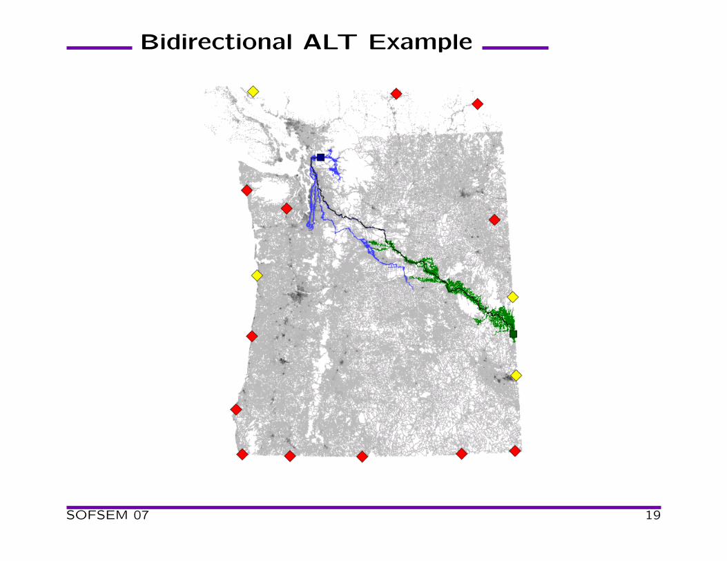
Bidirectional ALT Example
SOFSEM 07 19
Experimental Results
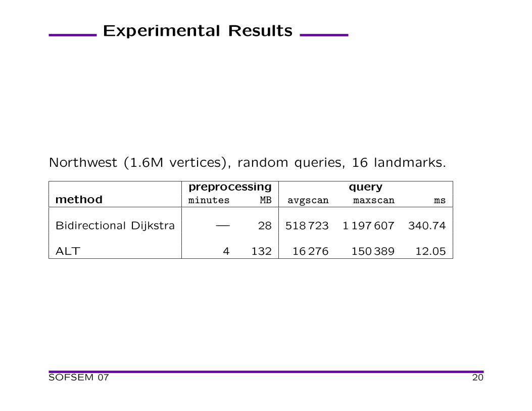
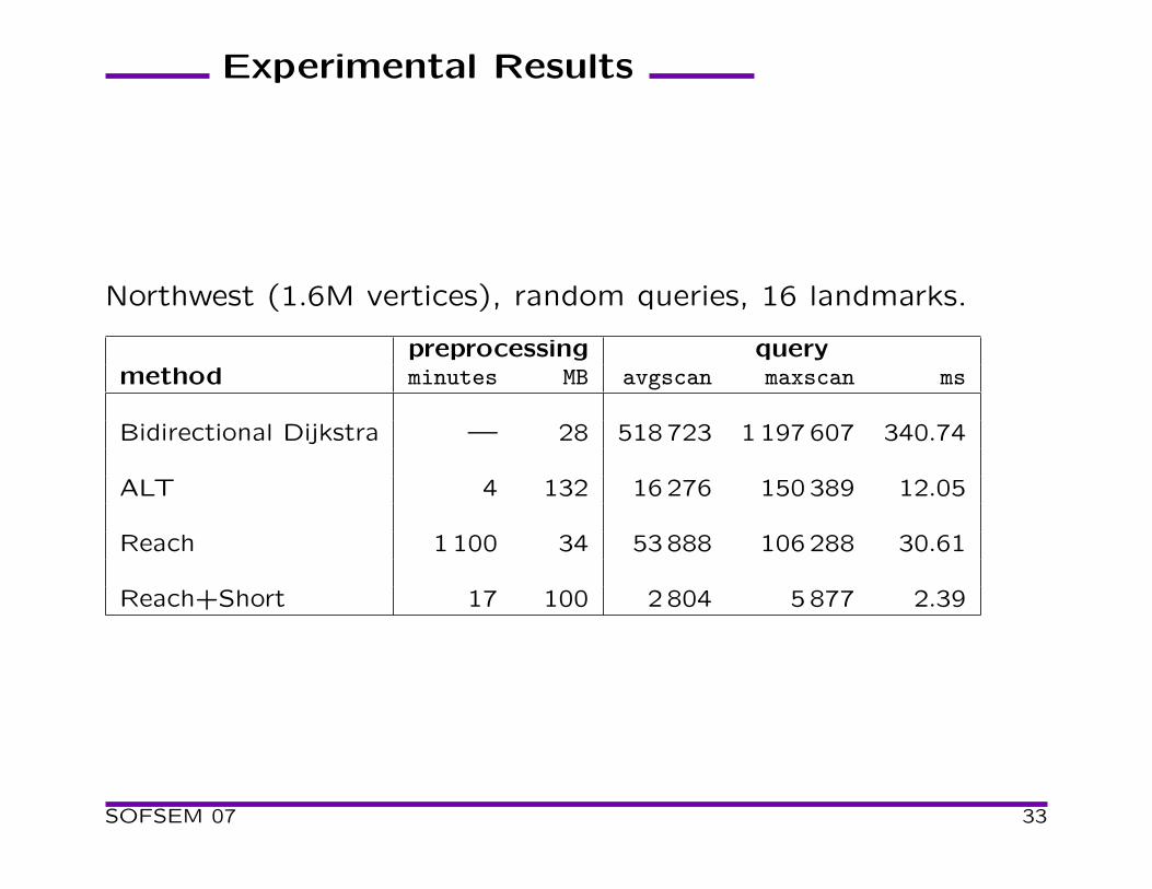
Northwest (1.6M vertices), random queries, 16 landmarks.
preprocessing querymethod minutes MB avgscan maxscan ms
Bidirectional Dijkstra — 28 518723 1197607 340.74
ALT 4 132 16276 150389 12.05
SOFSEM 07 20
Reaches
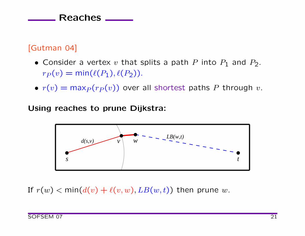
[Gutman 04]
• Consider a vertex v that splits a path P into P1 and P2.
rP (v) = min(ℓ(P1), ℓ(P2)).
• r(v) = maxP (rP (v)) over all shortest paths P through v.
Using reaches to prune Dijkstra:
LB(w,t)d(s,v) wv
ts
If r(w) < min(d(v) + ℓ(v, w), LB(w, t)) then prune w.
SOFSEM 07 21
Obtaining Lower Bounds
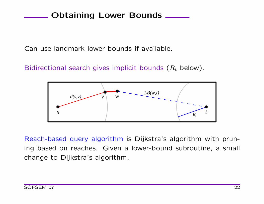
Can use landmark lower bounds if available.
Bidirectional search gives implicit bounds (Rt below).
Rt
LB(w,t)d(s,v) wv
ts
Reach-based query algorithm is Dijkstra’s algorithm with prun-
ing based on reaches. Given a lower-bound subroutine, a small
change to Dijkstra’s algorithm.
SOFSEM 07 22
Computing Reaches
• A natural exact computation uses all-pairs shortest paths.
• Overnight for 0.3M vertex graph, years for 30M vertex graph.
• Have a heuristic improvement, but it is not fast enough.
• Can use reach upper bounds for query search pruning.
Iterative Approximation Algorithm: [Gutman 04]
• Use partial shortest path trees of depth O(ǫ) to bound reaches
of vertices v with r(v) < ǫ.
• Delete vertices with bounded reaches, add penalties.
• Increase ǫ and repeat.
Query time does not increase much; preprocessing faster but still
not fast enough.
SOFSEM 07 23
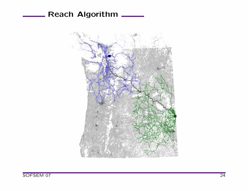
Reach Algorithm
SOFSEM 07 24
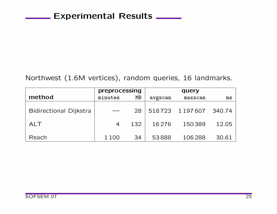
Experimental Results
Northwest (1.6M vertices), random queries, 16 landmarks.
preprocessing querymethod minutes MB avgscan maxscan ms
Bidirectional Dijkstra — 28 518723 1197607 340.74
ALT 4 132 16276 150389 12.05
Reach 1100 34 53888 106288 30.61
SOFSEM 07 25
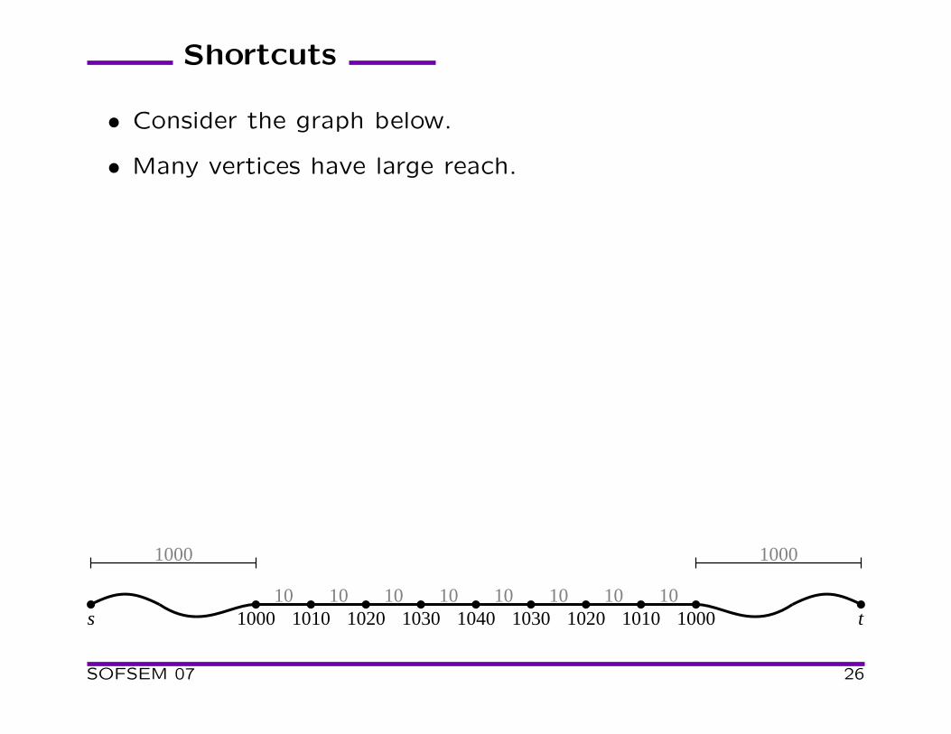
Shortcuts
• Consider the graph below.
• Many vertices have large reach.
10001000
1010101010101010100010101020103010401030102010101000 ts
SOFSEM 07 26

Shortcuts
• Consider the graph below.
• Many vertices have large reach.
• Add a shortcut arc, break ties by the number of hops.
10001000
1010101010101010
80
ts
SOFSEM 07 27
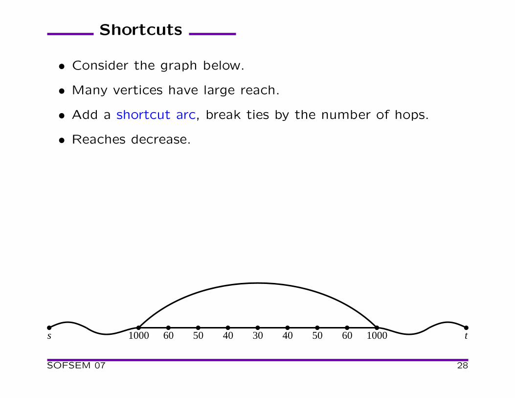
Shortcuts
• Consider the graph below.
• Many vertices have large reach.
• Add a shortcut arc, break ties by the number of hops.
• Reaches decrease.
1000605040304050601000 ts
SOFSEM 07 28
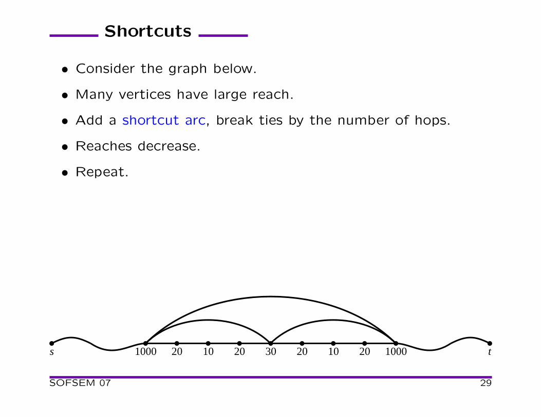
Shortcuts
• Consider the graph below.
• Many vertices have large reach.
• Add a shortcut arc, break ties by the number of hops.
• Reaches decrease.
• Repeat.
1000201020302010201000 ts
SOFSEM 07 29
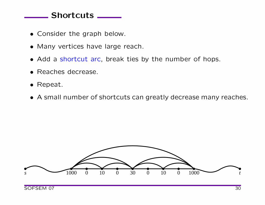
Shortcuts
• Consider the graph below.
• Many vertices have large reach.
• Add a shortcut arc, break ties by the number of hops.
• Reaches decrease.
• Repeat.
• A small number of shortcuts can greatly decrease many reaches.
100001003001001000 ts
SOFSEM 07 30
Shortcuts
[Sanders & Schultes 05].
• During preprocessing we shortcut degree 2 vertices every
time ǫ is updated.
• Shortcuts greatly speed up preprocessing.
• Shortcuts speed up queries.
• Shortcuts require more space (extra arcs, auxiliary info.)
SOFSEM 07 31
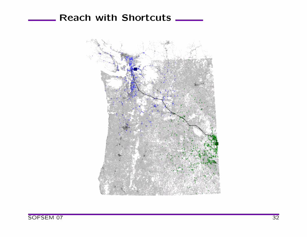
Reach with Shortcuts
SOFSEM 07 32
Experimental Results
Northwest (1.6M vertices), random queries, 16 landmarks.
preprocessing querymethod minutes MB avgscan maxscan ms
Bidirectional Dijkstra — 28 518723 1197607 340.74
ALT 4 132 16276 150389 12.05
Reach 1100 34 53888 106288 30.61
Reach+Short 17 100 2804 5877 2.39
SOFSEM 07 33
Reaches and ALT
• ALT computes transformed and original distances.
• ALT can be combined with reach pruning.
• Careful: Implicit lower bounds do not work, but landmark
lower bounds do.
• Shortcuts do not affect landmark distances and bounds.
SOFSEM 07 34
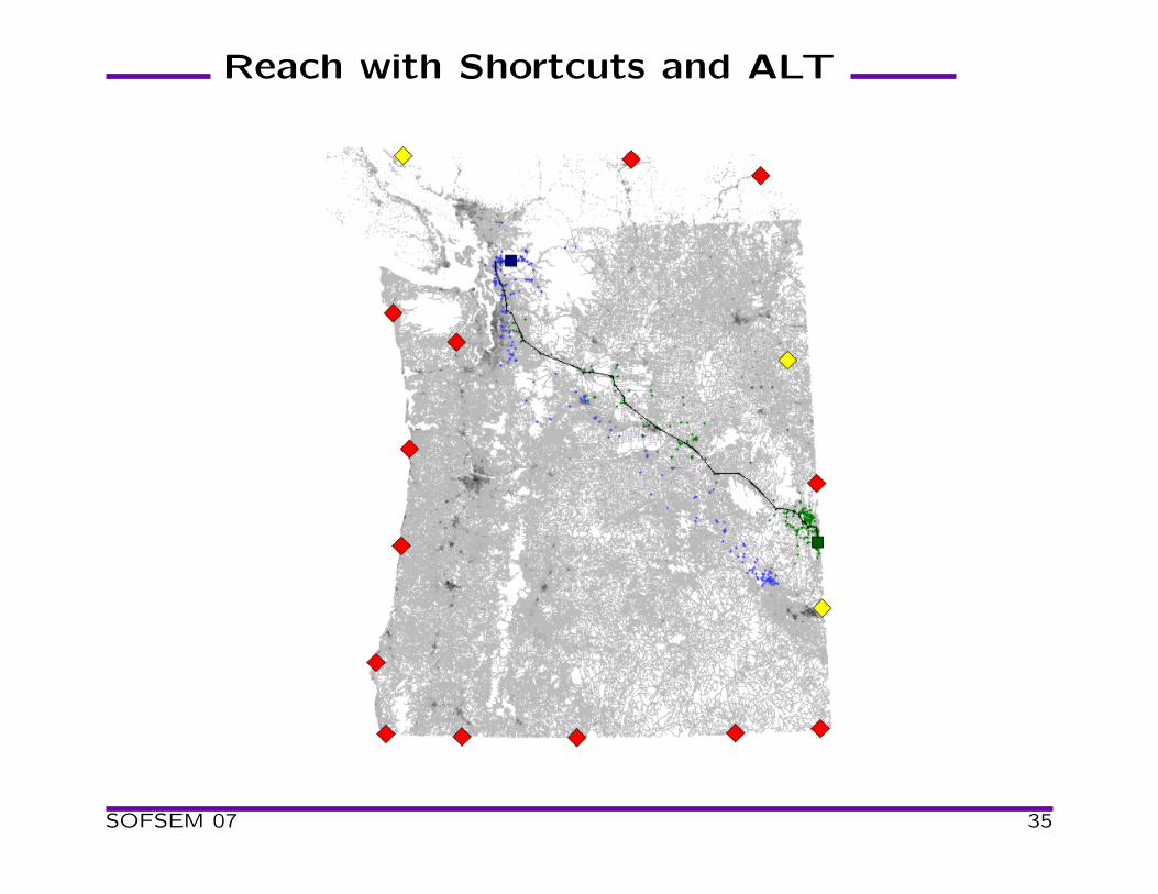
Reach with Shortcuts and ALT
SOFSEM 07 35
Experimental Results
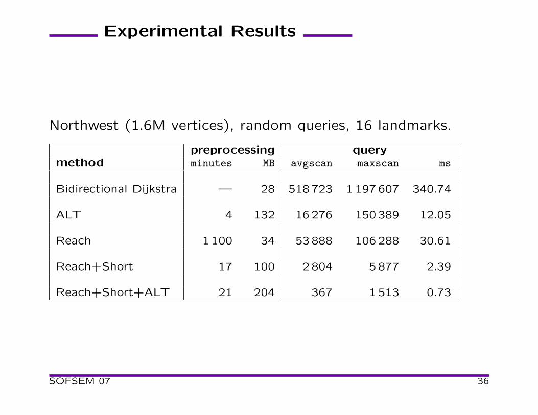
Northwest (1.6M vertices), random queries, 16 landmarks.
preprocessing querymethod minutes MB avgscan maxscan ms
Bidirectional Dijkstra — 28 518723 1197607 340.74
ALT 4 132 16276 150389 12.05
Reach 1100 34 53888 106288 30.61
Reach+Short 17 100 2804 5877 2.39
Reach+Short+ALT 21 204 367 1513 0.73
SOFSEM 07 36
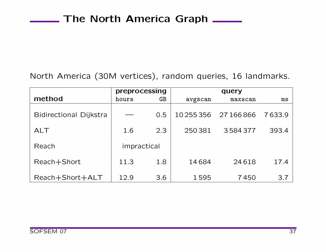
The North America Graph
North America (30M vertices), random queries, 16 landmarks.
preprocessing querymethod hours GB avgscan maxscan ms
Bidirectional Dijkstra — 0.5 10255356 27166866 7633.9
ALT 1.6 2.3 250381 3584377 393.4
Reach impractical
Reach+Short 11.3 1.8 14684 24618 17.4
Reach+Short+ALT 12.9 3.6 1595 7450 3.7
SOFSEM 07 37
Recent Improvements
• Better shortcuts [Sanders & Schultes 06]: replace small de-
gree vertices by cliques. For constant degree bound, O(n)
arcs are added.
• Improved locality (sort by reach).
• For RE, factor of 3− 12 improvement for preprocessing and
factor of 2 − 4 for query times.
SOFSEM 07 38
Recent Improvements (cont.)
Reach-aware landmarks:
• Store landmark distances only for high-reach vertices (e.g.,
5%).
• For low-reach vertices, use the closest high-reach vertex to
compute lower bounds.
• Can use freed space for more landmarks, improve both space
and time.
Practical even on the North America graph (30M vertices):
• ≈ 1ms. query time on a server.
• ≈ 6sec. query time on a Pocket PC with 4GB flash card.
• Better for local queries.
SOFSEM 07 39
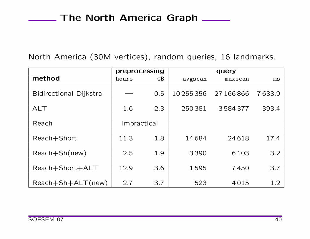
The North America Graph
North America (30M vertices), random queries, 16 landmarks.
preprocessing querymethod hours GB avgscan maxscan ms
Bidirectional Dijkstra — 0.5 10255356 27166866 7633.9
ALT 1.6 2.3 250381 3584377 393.4
Reach impractical
Reach+Short 11.3 1.8 14684 24618 17.4
Reach+Sh(new) 2.5 1.9 3390 6103 3.2
Reach+Short+ALT 12.9 3.6 1595 7450 3.7
Reach+Sh+ALT(new) 2.7 3.7 523 4015 1.2
SOFSEM 07 40
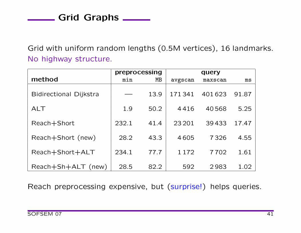
Grid Graphs
Grid with uniform random lengths (0.5M vertices), 16 landmarks.
No highway structure.
preprocessing querymethod min MB avgscan maxscan ms
Bidirectional Dijkstra — 13.9 171341 401623 91.87
ALT 1.9 50.2 4416 40568 5.25
Reach+Short 232.1 41.4 23201 39433 17.47
Reach+Short (new) 28.2 43.3 4605 7326 4.55
Reach+Short+ALT 234.1 77.7 1172 7702 1.61
Reach+Sh+ALT (new) 28.5 82.2 592 2983 1.02
Reach preprocessing expensive, but (surprise!) helps queries.
SOFSEM 07 41
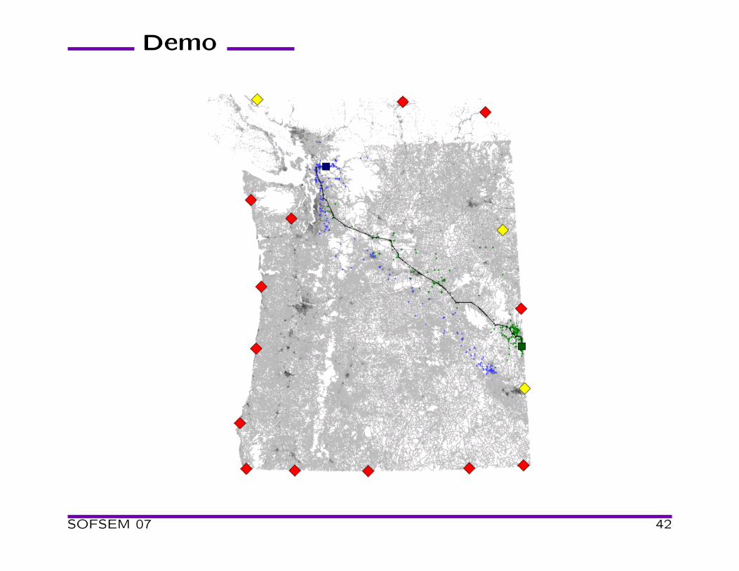
Demo
SOFSEM 07 42
Concluding Remarks
• Recent progress [Bast et. al 06], improvements with Sanders
and Schultes.
• Preprocessing heuristics work well on road networks.
• How to select good shortcuts? (Road networks/grids.)
• For which classes of graphs do these techniques work?
• Need theoretical analysis for interesting graph classes.
• Interesting problems related to reach, e.g.◦ Is exact reach as hard as all-pairs shortest paths?
◦ Constant-ratio upper bounds on reaches in O(m) time.
• Dynamic graphs.
SOFSEM 07 43
![Reach for A : Shortest Path Algorithms with Preprocessing · The bidirectional algorithm [5, 13, 38] alternates between running the forward and reverse versions of Dijkstra’s algorithm,](https://img.pdfslide.net/doc/110x75/5e63ac3a68f8d538d9099551/reach-for-a-shortest-path-algorithms-with-preprocessing-the-bidirectional-algorithm.jpg)