POISSON GEOMETRY AND REPRESENTATIONS OF PI 4 …

POISSON GEOMETRY AND REPRESENTATIONS

OF PI 4-DIMENSIONAL SKLYANIN ALGEBRAS

CHELSEA WALTON, XINGTING WANG, AND MILEN YAKIMOV

Abstract. Take S to be a 4-dimensional Sklyanin (elliptic) algebra that is module-

finite over its center Z; thus, S is PI. Our first result is the construction of a Poisson

Z-order structure on S such that the induced Poisson bracket on Z is non-vanishing.

We also provide the explicit Jacobian structure of this bracket, leading to a description

of the symplectic core decomposition of the maximal spectrum Y of Z. We then classify

the irreducible representations of S by combining (1) the geometry of the Poisson order

structures, with (2) algebro-geometric methods for the elliptic curve attached to S, along

with (3) representation-theoretic methods using line and fat point modules of S. Along

the way, we improve results of Smith and Tate obtaining a description the singular locus

of Y for such S. The classification results for irreducible representations are in turn

used to determine the zero sets of the discriminants ideals of these algebras S.

Contents

1. Introduction 2

1.1. Overview of Sklyanin algebras and results in the paper 2

1.2. Poisson orders, classification of symplectic cores and Azumaya loci 3

1.3. On irreducible representations of PI 4-dimensional Sklyanin algebras 5

2. Preliminary results on 4-dimensional Sklyanin algebras S 7

2.1. Noncommutative geometry of S 7

2.2. Center of S 10

2.3. Symmetries of S and of their centers 11

3. Singular loci of the maximal spectra of the centers of the PI 4-dimensional

Sklyanin algebras S 15

3.1. For PIdeg(S) odd 18

3.2. For PIdeg(S) even 22

4. Background material on Poisson orders and specialization 25

4.1. Poisson orders and specialization 25

4.2. Symplectic cores and the Brown-Gordon theorem 27

5. A specialization setting for 4-dimensional Sklyanin algebras 27

6. Poisson orders on PI 4-dimensional Sklyanin algebras S 30

6.1. Construction of Poisson orders 30

6.2. Derivations of PI S 32

6.3. Proof of Theorem 6.10, nontriviality of Poisson order structure on S 35

2010 Mathematics Subject Classification. 14A22, 16G99, 17B63, 81S10.Key words and phrases. 4-dimensional Sklyanin algebra, Poisson order, Azumaya locus, singular locus,

irreducible representation.Walton and Yakimov are partially supported by respective NSF grants #1663775 and #1601862. Wang

is partially supported by an AMS-Simons travel grant.

1

2 CHELSEA WALTON, XINGTING WANG, AND MILEN YAKIMOV

7. The Jacobian structure of Poisson orders on PI 4-dimensional Sklyanin

algebras 36

8. On the representation theory of PI 4-dimensional Sklyanin algebras S 38

8.1. Irreducible representations of PI S of maximum dimension 39

8.2. Irreducible representations of PI S of intermediate dimension 42

8.3. Discriminant ideals of the PI 4-dimensional Sklyanin algebras 47

References 48

Index of Notation 51

1. Introduction

1.1. Overview of Sklyanin algebras and results in the paper. Sklyanin algebras

are quadratic algebras that play a major role in the Artin-Schelter-Tate-van den Bergh’s

classification of noncommutative projective spaces [2, 3, 4, 5] and the Feigin-Odeskii’s

investigation of elliptic algebras [23, 24]. These directions were motivated by Sklyanin’s

work [35] on quantum integrable systems, in which he introduced the algebras now known

as 4-dimensional Sklyanin algebras and studied their representations with applications to

the quantum inverse problem method in quantum and statistical mechanics. Since then,

n-dimensional versions of Sklyanin’s algebras were introduced for n ≥ 3 and have arisen

in numerous areas including: deformation-quantization, non-commutative geometry, and

quantum groups and R-matrices; see, for instance, the reviews [8, 30, 41] and the refer-

ences within.

In terms of their representation theory, Sklyanin algebras fall into one of two classes–

those that are module-finite over their center so that they satisfy a polynomial identity

(or, are PI), or otherwise.

(A) In the generic (non-PI) case, a Sklyanin algebra is infinite-module over its center.

Its representation theory can be viewed in parallel with the representations of quantum

groups at non-roots of unity and Lie algebras over fields of characteristic 0. Sklyanin

algebras are more complicated than the other two classes because they do not have PBW

bases in the usual sense and thus one cannot use the classical methods of standard modules

(for instance Verma modules in the case of the categories O). However, Artin-Schelter-

Tate-van den Bergh have developed powerful projective algebro-geometric methods that

can be applied to analyze the representations of these algebras via algebraic geometry of

elliptic curves. Such methods were further developed in works of Levasseur-Smith [29],

Smith-Staniszkis [38], and Staniszkis [42] to achieve results on the noncommutative pro-

jective algebraic geometry of irreducible representations of generic 4-dimensional Sklyanin

algebras.

(B) Representations of PI Sklyanin algebras can be viewed in parallel with represen-

tations of quantum groups at roots of unity and modular representations of Lie algebras.

This case is substantially harder than setting (A). In this paper we unify the algebro-

geometric methods for Sklyanin algebras with Poisson geometric methods for quantum

groups at roots of unity, to

(1) construct nontrivial structures of Poisson orders on all PI 4-dimensional Sklyanin

algebras, and

(2) explicitly classify their irreducible representations and describe their dimensions.

POISSON GEOMETRY AND REPRESENTATIONS OF SKLYANIN ALGEBRAS 3

Smith [36] has obtained a number of important results in the direction (2) by exclusively

using algebro-geometric methods. Pertaining to direction (1), De Concini-Kac-Procesi

[19, 20] pioneered the applications of Poisson geometry in representation theory of PI

algebras, for the cases of quantized universal enveloping algebras and quantum function

algebras at roots of unity. This approach was axiomatized by Brown-Gordon [13] in the

theory of Poisson orders and was applied to other families of algebras with PBW bases,

such as the symplectic reflection algebras. A Poisson order is an algebra A which is

module-finite over its center Z, and such that Z admits a Poisson structure for which

all Hamiltonian derivations of Z can be extended to derivations of A. The punchline

of the construction is that Brown and Gordon used the latter extension to construct an

isomorphism A/(mA) ∼= A/(nA) for m, n ∈ maxSpec(Z) in the same symplectic core,

[13, 19, 20]. This provides general Poisson geometric tools to organize the irreducible

representations of A into families that behave in similar ways (e.g., that have the same

dimension).

We use previous algebro-geometric results on the PI 4-dimensional Sklyanin algebras

S, [2, 3, 4, 5, 37, 39, 40], to prove that every such algebra has a nontrivial structure of

Poisson order. We classify the symplectic cores of Z(S) and obtain from it a concrete

description of the Azumaya locus of S. We then link the developed Poisson geometry

back to the algebro-geometric approach to the representation theory of S, [27, 29, 36],

to classify the irreducible representations of S and to describe their dimensions. See

Sections 1.2 and 1.3 for more details.

Poisson structures on commutative algebras which arise as semiclassical limits of elliptic

algebras were studied by Odesskiı-Feıgin [23], Pym-Schedler [31], and others. The novelty

in our work is the noncommutative extension of Poisson algebras to Poisson orders for all

PI 4-dimensional Sklyanin algebras S, which is the key feature that is needed to approach

the representation theory of S.

In our previous work [43] we have obtained similar results for the PI 3-dimensional

Sklyanin algebras. The 4-dimensional case turns out to be substantially more challenging,

and requires new approaches at various steps. We indicate those throughout the paper.

On the other hand, we develop methods that can be applied in far greater generality than

4-dimensional Sklyanin algebras, for instance, connected N-graded algebras T containing

a regular sequence of central elements Ω1, . . . ,Ωm such that T/(TΩ1 + · · · + TΩm) is

isomorphic to a twisted homogeneous coordinate ring of an elliptic curve; such results are

highlighted throughout our work.

We use the solution of the classification problem (2) for irreducible representations of

the algebras S to fully determine the zero sets of all of their discriminant ideals. This

will likely have further applications in relation to recent work of Bell-Zhang [7], Ceken-

Palmieri-Wang-Zhang [16], and Brown-Yakimov [15].

1.2. Poisson orders, classification of symplectic cores and Azumaya loci. We

work over an algebraically closed base field k of characteristic 0. The projective algebro-

geometric data attached to a 4-dimensional Sklyanin algebra S are: an elliptic curve E

in P3, an invertible sheaf L on E and an automorphism of σ of E given by a translation

of a point τ ∈ E. See Section 2.1 for details.

One nice fact we have is that S is module-finite over its center if and only if the

automorphism σ attached to S has finite order. In this case S is PI and the PI degree


of S (which is a sharp upper bound on the dimension of irreducible representations of S)

is equal to |σ|; see Proposition 2.12. So, consider the following standing hypothesis and

notation used throughout this work.

Hypothesis 1.1. [S, Z, n, s] Let S be a 4-dimensional Sklyanin algebra, and (with the

exception of Sections 2 and 5) assume that S is module-finite over its center Z so that S

is PI. For the geometric data (E,L, σ) attached to S mentioned above, let n denote |σ|,which is equal to the PI degree of S when |σ| is finite. Also, let s := n/(n, 2).

In this work, we do not consider the cases when n divides 4, as done typically in works

on 4-dimensional Sklyanin algebras [29, 38, 42]. (See, e.g., [42, proof of Lemma 2.1].)

Smith and Tate [39] proved that the center Z(S) of every PI 4-dimensional Sklyanin

algebra S is generated by four elements z0, . . . , z3 of degree n and two elements g1, g2 of

degree 2, subject to two relations F1 and F2 of degree 2n. Set

Y := maxSpec(Z(S)) and Yγ1,γ2 := Y ∩ V(g1 − γ1, g2 − γ2), for γ1, γ2 ∈ k.

Denote by Y sing the singular locus of Y . Further, (Yγ1,γ2)sing denotes the singular locus

of the subvariety Yγ1,γ2 and

(Y sing)γ1,γ2 := Y sing ∩ Yγ1,γ2 .

Here, Y sing =⋃γ1,γ2∈k(Y sing)γ1,γ2 , which is contained in but not necessarily equal to⋃

γ1,γ2∈k(Yγ1,γ2)sing.

Our first main result constructs a nontrivial Poisson order on S, classifies the sym-

plectic cores of its center Z(S) = k[z0, z1, z2, z3, g1, g2]/(F1, F2), and fully determines the

Azumaya locus of S.

Theorem 1.2. [Theorems 7.5 and 8.1, Corollary 7.7, Proposition 8.8] For all 4-dimensional

Sklyanin algebras S satisfying Hypothesis 1.1 the following hold:

(1) S admits a nontrivial structure of Poisson order for which

(a) the induced Poisson structure on the center Z(S) is of Jacobian form in the

sense of (7.4) in terms of two potentials taken to be F1 and F2, while

(b) g1, g2 lie in the Poisson center of Z(S).

(2) The corresponding symplectic core stratification of the Poisson variety Y are

(a) 2-dimensional cores: (Yγ1,γ2)smooth := Yγ1,γ2 \ (Yγ1,γ2)sing for γ1, γ2 ∈ k;

(b) 0-dimensional cores: points in Y symp0 :=

⋃γ1,γ2∈k(Yγ1,γ2)sing; these are the

points on which the Poisson bracket on Y in part (1) vanishes.

(3) Y sing ⊆ Y symp0 , sometimes with strict containment, and they both have codimen-

sion ≥ 2 in Y ;

(4) The Azumaya locus of S coincides with the smooth locus Y \ Y sing in Y .

The above result can be thought as a generalization of the previous work done for

PI 3-dimensional Sklyanin algebras. There are a number of complications that arise in

the 4-dimensional case compared to the 3-dimensional one. The first one is that in the

4-dimensional case we have Y sing ( Y symp0 when the order n of σ is odd; in other words

the set of symplectic points Y symp0 of the Poisson variety Y is larger than its singular

locus. Indeed in that case Y symp0 is the union of Y sing plus four nodal curves meeting at

the origin; this is proved in Theorem 3.13.


See Figure 1 in Section 3 for an illustration of the n is odd case, where Y sing ( Y symp0

as discussed above. On the other hand, Figure 2 in Section 3 illustrates the n even case,

when Y sing and Y symp0 coincide.

As mentioned in Section 1.1, the proof of the existence of nontrivial Poisson order

structure on S relies on the previous algebro-geometric results for S and a method of

higher order specialization developed in [43]. The precise (Jacobian) form of the Poisson

structure on Z(S) is derived from the property that g1, g2 are in the Poisson center of

Z(S) and from Stafford’s result [40] that S is a maximal order.

The proof of Theorem 1.2(4) faces a second major difficulty compared to the 3-

dimensional case. In the latter case, the symplectic cores of Z(S) of maximal dimension

have codimension 1 which was used to show that all of them are in the Azumaya locus of

S by incorporating the automorphism group of S. This strategy fails in the 4-dimensional

case since the leaves have codimension 2 while the automorphism group of S is still 1-

dimensional. Our strategy for the proof of part (4) is to take a much more roundabout

route. Firstly, we consider the factors

S[κ1:κ2] := S/(κ1g1 − κ2g2)S, for [κ1 : κ2] ∈ P1k

which all turn out to be Noetherian PI domains of the same PI degree as S. We show that

the maximal spectra of their centers are canonically isomorphic to Poisson subvarieties

of Y with the property that the symplectic leaves in them of maximal dimension have

codimension 1 in Y . Now, by applying Brown and Gordon’s Poisson order result [13]

(as discussed in Section 4.2) to the symplectic core stratification of the centers of the

algebras S[κ1:κ2] and using the density of their Azumaya loci, we conclude that all the

points in the 2-dimensional cores (Yγ1,γ2)smooth lie in the Azumaya locus of S. Then the

coincidence of the Azumaya and smooth locus of S follows from a general result of Brown

and Goodearl [11] since the non-Azumaya locus of S contained in Y symp0 has codimension

≥ 2 in Y . Thus, Poisson geometry was employed primarily to establish the codimension

≥ 2 fact, for which there are no other known methods.

The novelty of the 4-dimensional Sklyanin algebras of odd PI degree is that their

Azumaya loci intersects nontrivially the varieties of symplectic points Y symp0 of Y .

1.3. On irreducible representations of PI 4-dimensional Sklyanin algebras. For

y ∈ Y , denote by my the corresponding maximal ideal of Z(S). It follows from Theorem

1.2 that

• For y ∈ Y \Y sing, S/myS ∼= Mn(k), and thus, up to isomorphism, there is pre-

cisely one irreducible representation of S with central annihilator my and this

representation has dimension n.

Recall that n denotes the order of the automorphism σ of the elliptic curve attached to

S; it equals the PI degree of S. It is a simple fact that

• For y = 0, S/myS is a local algebra, and thus, up to isomorphism, S has precisely

one irreducible representation with central annihilator m0 and this representation

is the trivial representation of dimension 1.

To achieve results on irreducible representations of intermediate dimension, we first

use the explicit structure of the center Z(S) and its link with the geometry of the elliptic

curve E to describe the singular locus Y sing of S.


Theorem 1.3. [Theorems 3.13, 3.16] Let S be a 4-dimensional Sklyanin algebra satisfying

Hypothesis 1.1. Denote by E2 the subgroup of 2-torsion points of E.

(1) If n is odd, then the singular locus of Y is the union of 2(n − 1) nodal curves

C(ω + kτ),

Y sing =⋃ω∈E2

0≤k≤n−2

C(ω + kτ),

defined in Lemma 3.12, which only meet at the origin, as depicted in Figure 1.

(2) If n = 2s is even, then Y sing is the union of two explicitly defined subvarieties

Y sing1 and Y sing

2 in Theorem 3.16, which only meet at the origin, as depicted in

Figure 2. When k = C, they contain the nodal curves

C(ω + kτ) for ω ∈ E2, 0 ≤ k ≤ s− 1

described in Notation 8.27.

The proof of Theorem 1.3 relies on the geometry of line modules and fat point modules

of S, extending results of [29, 39].

Next, we fully classify the irreducible representations of S of intermediate dimension

and describe their dimensions. Along the way, using the action of Heisenberg group H4 of

order 64 on S, we determine the exact form of the Smith-Tate defining relations F1 and F2

of the center Z(S) when n is even, which is of independent interest (see Proposition 2.23

below).

Theorem 1.4. [Theorems 8.29, 8.30] Let S be a complex 4-dimensional Sklyanin algebra

satisfying Hypothesis 1.1. Denote by Irrd S the isomorphism classes of all d-dimensional

irreducible representations of S. Recall the notation above.

(1) If PIdeg(S) = n is odd, then we have the following maps via central annihilators.

Irrn S1:1 // // Y smooth = (Y \ Y sing)

Irrk+1 S t Irrn−1−k S2:1 // // (C(ω + kτ) = C(ω + (n− 2− k)τ)) \ 0, 0 ≤ k ≤ n− 2

Irr1 S1:1 // // 0

(2) If PIdeg(S) = n = 2s is even, then we have the following maps via central anni-hilators.

Irrn S1:1 // // Y smooth = (Y \ Y sing)

Irrs S2:1 // // Y sing \

⋃ω∈E2,0≤k≤s−2 C(ω + kτ)

Irrk+1 St Irrs−1−k S4:1 // // (C(ω + kτ) = C(ω + sτ + (s− 2− k)τ)) \ 0, 0 ≤ k ≤ s− 2;

Irr1 S1:1 // // 0

Over complex numbers k = C, Sklyanin constructed in [35] for each ω ∈ E2 and

k ∈ N∪0, a representation V (ω+ kτ) over S in a certain (k+ 1)-dimensional subspace

of theta functions of order 2k; see [38, Section 3] for details. These representations were

proved later by Smith and Staniszkis to be irreducible whenever k < s [38, Theorem 3.6].

Our next result shows that every irreducible representation of S of intermediate dimension


< s is a scalar twist of V (ω+kτ)λ for some λ ∈ k such that V (ω+kτ)λ equals V (ω+kτ)

as vector spaces and si ·λ v = λisiv for any homogeneous element si in S of degree i and

v ∈ V (ω + kτ)λ.

Theorem 1.5. [Theorems 8.29, 8.30] Let S be a complex 4-dimensional Sklyanin alge-

bra satisfying Hypothesis 1.1. Then S has irreducible representations of each dimension

1, 2, 3, . . . , n (= s) if n is odd, and of each dimension 1, 2, 3, . . . , n2 (= s), n if n is even.

Moreover, the nontrivial irreducible representations of intermediate dimension < s are

given by scalar twists of V (ω + kτ) for all ω ∈ E2 and 0 ≤ k ≤ s− 2.

To prove Theorems 1.4 and 1.5, we use the classification of fat points of S by Smith

in [36], a number of other representation-theoretic results of Levasseur, Le Bruyn, Smith

and Staniszkis [27, 29, 36, 38], and part (4) of Theorem 1.2 that the non-Azumaya part of

Z(S) is Y sing. In particular, we apply the deep connections between fat point modules,

C× × PGLd-stabilizers of irreducible representations, and C∗-families of irreducible rep-

resentations of a graded algebra within the framework of the noncommutative projective

algebraic geometry of S.

Finally, Theorem 8.31 in Section 8.3 contains the aforementioned results on the de-

scription of the zero sets of the discriminant ideals of the algebras S.

Remark 1.6. Note that Theorem 1.4 makes precise the representation-theoretic con-

nection between the PI 4-dimensional Sklyanin algebras and the quantized enveloping

algebra Uq(SU(2)) at q a root of unity, as introduced initially in the physics literature.

Namely, the main result of Roche-Arnaudon [33] is that when q is a root of unity of order

m, then Uq(SU(2)) has d-dimensional irreducible representations for all 1 ≤ d ≤ m when

m is odd, and has d-dimensional irreducible representations for all 1 ≤ d ≤ m2 and d = m

when m is even. They also show that Uq(SU(2)) arises as a ‘trigonometric limit’ of a

4-dimensional Sklyanin algebra S. Connections between S and Uq(SU(2)) (or rather,

Uq(sl2)) are also discussed in work of Smith and Stafford [37, Section 1].

Acknowledgements. The authors thank S. Paul Smith for generously making available

his 1993 work [36] via private communication and for also making it available for public

use recently on the ArXiv e-print service.

2. Preliminary results on 4-dimensional Sklyanin algebras S

We provide in this section background material on (the noncommutative projective

algebraic geometry of) 4-dimensional Sklyanin algebras. This includes a discussion of

various ring-theoretic and homological properties of these algebras, which were established

by Smith-Stafford [37]. We also provide a detailed analysis of the center and symmetries

of 4-dimensional Sklyanin algebras, which will play a key role in the rest of the paper. This

analysis extends results of Smith-Tate [39], Smith-Staniszkis [38], and Chirvasitu-Smith

[17].

In this section, we do not assume that the 4-dimensional Sklyanin algebras S are PI.

2.1. Noncommutative geometry of S. Here, we recall the definition and properties

of the 4-dimensional Sklyanin algebras and the corresponding twisted homogeneous co-

ordinate rings.


Definition 2.1. [S, S(α, β, γ), xi] [37] Take α, β, γ ∈ k so that

α+ β + γ + αβγ = 0 [⇔ (1 + α)(1 + β)(1 + γ) = (1− α)(1− β)(1− γ)],(2.2)

(α, β, γ) 6∈ (−1, 1, γ), (α,−1, 1), (1, β,−1).(2.3)

Then the (regular) 4-dimensional Sklyanin algebra S := S(α, β, γ) are k-algebras gener-

ated by noncommuting variables x0, x1, x2, x3 of degree one, subject to the following

relations

x0x1 − x1x0 = α(x2x3 + x3x2), x0x1 + x1x0 = x2x3 − x3x2,

x0x2 − x2x0 = β(x3x1 + x1x3), x0x2 + x2x0 = x3x1 − x1x3,

x0x3 − x3x0 = γ(x1x2 + x2x1), x0x3 + x3x0 = x1x2 − x2x1.

These algebras come equipped with geometric data that is used to establish many of

their nice ring-theoretic, homological, and representation-theoretic properties. To start,

take a N-graded algebra A = A0 ⊕ A1 ⊕ A2 ⊕ · · · with A0 = k, and recall that an

A-point module is a cyclic, graded left A-module with Hilbert series (1 − t)−1. These

modules play the role of points in noncommutative projective algebraic geometry and

the parameterization of A-point modules is referred to as the point scheme of A. See [8,

Chapter I, Section 3] for more details.

Definition-Lemma 2.4. [E, E, φ1, φ2, vi, ei, σ, τ ] [37, Section 2] The point scheme of

the 4-dimensional Sklyanin algebra S = S(α, β, γ) is given by the union E of an elliptic

curve E := V (φ1, φ2) ⊆ P3[v0:v1:v2:v3], where

φ1 = v20 + v2

1 + v22 + v2

3 and φ2 = 1−γ1+α v2

1 + 1+γ1−β v

22 + v2

3,

with the four points

e0 := [1 : 0 : 0 : 0], e1 := [0 : 1 : 0 : 0], e2 := [0 : 0 : 1 : 0], e3 := [0 : 0 : 0 : 1].

The automorphism σ = σαβγ of E attached to S fixes each of the four points ei and on

E it is defined on a dense open subset by

(2.5) σ :

v0

v1

v2

v3

7→−2αβγv1v2v3 − v0(−v2

0 + βγv21 + αγv2

2 + αβv23)

2αv0v2v3 + v1(v20 − βγv2

1 + αγv22 + αβv2

3)

2βv0v1v3 + v2(v20 + βγv2

1 − αγv22 + αβv2

3)

2γv0v1v2 + v3(v20 + βγv2

1 + αγv22 − αβv2

3)

·The automorphism σ of E is given by translation by a point of E; call this point τ . The

triple (E, OP3(1)|E , σ) is referred to as the geometric data of S.

Using this data, we consider a noncommutative coordinate ring of E; its generators

are sections of the invertible sheaf OP3(1)|E and its multiplication depends on the auto-

morphism σ. The general construction is given as follows.

Definition 2.6. [Li] [6] Given a projective scheme X, an invertible sheaf L on X, and an

automorphism σ of X, the twisted homogeneous coordinate ring attached to this geometric

data is a graded k-algebra

B(X,L, σ) =⊕

i≥0Bi, where Bi := H0(X,Li)

with L0 = OX , L1 = L, and Li = L⊗Lσ ⊗ · · · ⊗Lσi−1for i ≥ 2. The multiplication map

Bi ⊗Bj → Bi+j is defined by bi ⊗ bj 7→ bibσij using Li ⊗ Lσ

i

j = Li+j .


Notation 2.7. [B, L] Let B denote the twisted homogeneous coordinate ring attached

to the geometric data (E,L, σ) from Definition-Lemma 2.4, where L := OP3(1)|E .

It is often useful to employ the following embedding of B in a skew-Laurent extension

of the function field of E.

Lemma 2.8. [2] Given (E,L, σ) from Definition-Lemma 2.4, extend σ to an automor-

phism of the field k(E) of rational functions on E by νσ(p) = ν(σ−1p) for ν ∈ k(E) and

p ∈ E. For any nonzero section w of L, that is, any degree 1 element of B, take D to be

the divisor of zeros of w, and let V denote H0(E,OE(D)) ⊂ k(E).

Then, the vector space isomorphism νw 7→ νt for ν ∈ V extends to an embedding of B

in k(E)[t±1;σ]. Here, tν = νσt for ν ∈ k(E).

Now the first step in obtaining nice properties of 4-dimensional Sklyanin algebras is to

use the result below.

Lemma 2.9. [g1, g2] [37, Lemma 3.3, Corollary 3.9, Theorem 5.4] The degree 1 spaces of

S and of B are equal and there is a surjective map from S to B, whose kernel is generated

by the two central degree 2 elements below

(2.10) g1 := −x20 + x2

1 + x22 + x2

3 and g2 := x21 + 1+α

1−β x22 + 1−α

1+γ x23

Moreover, g1, g2 is a central regular sequence in S.

Many good ring-theoretic and homological properties of S are obtained by lifting such

properties from the factor B, some of which are listed in the following result.

Proposition 2.11. [37, Theorem 5.5] [28, Corollary 6.7] The 4-dimensional Sklyanin

algebras are Noetherian domains of global dimension 4, they satisfy the Artin-Schelter

Gorenstein condition, along with the Auslander-regular and Cohen-Macaulay conditions,

and they have Hilbert series (1− t)−4.

The representation theory of both S and B depend on the geometric data (E,L, σ),

as illustrated by the following result.

Proposition 2.12. [n] Both of the algebras S and B = B(E,L, σ) ∼= S/(Sg1 + Sg2) are

module-finite over their center if and only if the automorphism σ has finite order. In

this case, both S and B satisfy a polynomial identity (i.e., are PI) and are of PI degree

n := |σ| <∞.

Proof. Suppose that the automorphism σ has finite order. Since L is ample and σ-ample,

the algebra B is module-finite over its center by [39, Corollary 2.3]. Moreover, so is S by

[39, Theorem 3.7(c)].

On the other hand, suppose that the automorphism σ has infinite order. Now the

center of S is the polynomial ring k[g1, g2] by [29, Proposition 6.12]. By comparing the

Hilbert series of S to that of k[g1, g2], we get S cannot be module-finite over its center

k[g1, g2].

To verify the last statement, note that B has PI degree n since it has a localization

isomorphic to k(E)[t±1;σ] (see Lemma 2.9) which in turn also has PI degree n. We will

also see later in Corollary 8.16 that all nontrivial irreducible representations of B have

dimension n, which provides another proof that B has PI degree n.

Finally, we see that the PI degree of S is also n as follows. First, PIdeg(S) ≥ PIdeg(B)

since B is a homomorphic image of S, and recall that PIdeg(B) = n from above. So,


it suffices to show that PIdeg(S) ≤ n. Take the central element defined in [36, (4-2)],

which is denoted by g later in Notation 3.9. (It is denoted by “c” in [36].) Let M be an

irreducible representation of S that is g-torsionfree. By [12, Theorem III.1.7], we know

the Azumaya locus of S is dense in maxSpec(Z). So we only need to show dimM ≤ n.

Recall s = n/(n, 2) and note that M is the quotient of a g-torsionfree fat point module F

of multiplicity s > 1 by [38, Lemma 4.1] and [36, Theorem 7.7(c)]. Fat point modules will

be discussed in detail in Section 8.2; they serve as representatives of the simple objects

of the quotient category S-qgr which is the category of graded S-modules modulo those

that are bounded above (Mn = 0 for all n 0). Now if n is odd, then F and its shift F [1]

are equivalent in S-qgr by [36, Corollary 8.7]. So, dim(M) ≤ mult(F ) = s = n by [36,

discussion after Proposition 3.19]. On the other hand, if n is even, then F and F [2] are

equivalent in S-qgr by [36, Proposition 5.4], and hence, dim(M) ≤ 2 mult(F ) = 2s = n

by [36, discussion after Proposition 3.19]. Thus, dim(M) ≤ n, as desired.

Remark 2.13. The claim that the PIdeg(S) = n first appeared in [36, Theorem 8.8(2)]

but the stronger statement that the ring S[c−1] in [36, Theorem 8.8(1)] is Azumaya (which

is used to prove [36, Theorem 8.8(2)]) is incorrect; there, “c” is our “g” in Notation 3.9.

We establish later in Theorem 8.1 and Theorem 3.16 that the Azumaya locus of S is

equal to the smooth locus of Y := maxSpec(Z(S)), and in the case when n is even, the

singular locus of Y does not lie in the hypersurface V(g). That is, there exist g-torsionfree

irreducible representations of S of dimension < n when n is even.

2.2. Center of S. As mentioned in the proof of Proposition 2.12, the center of a 4-

dimensional Sklyanin algebra S is equal to k[g1, g2] when n := |σ|=PIdeg(S) is infinite.

On the other hand, one expects that both S and B have a large center when the PI degree

of S is finite. We record here several results of Smith-Tate [39] pertaining to the center

Z of S when PIdeg(S) = n <∞.

Lemma 2.14. [E′′] [39, Corollary 2.8] Given the geometric data (E,L, σ) from Definition-

Lemma 2.4, suppose that |σ| =: n < ∞. Take E′′ := E/〈σ〉 so that E → E′′ is a cyclic

etale cover of degree n. Recall Lemma 2.8 and let D′′ be the image of D on E′′ and let

V ′′ denote H0(E′′,OE′′(D′′)).Then, the center of B is the intersection of B with k(E′′)[t±n], which is equal to

k[V ′′tn], and this is also a twisted homogeneous coordinate ring of E′′ for an embedding

of E′′ ⊆ P3.

Central elements of B lift to central elements of S as described below. We will identify

S1∼= B1 via the canonical projection mentioned in Lemma 2.9.

Definition 2.15. [s] [39] Take |σ| =: n <∞ and let s be the value n/(n, 2). A section of

B1 := H0(E,L) is called good if its divisor of zeros is invariant under σs and consists of

distinct points whose orbits under the group 〈σ〉 do not intersect. A good basis of B1 is

a basis that consists of good elements so that the s-th powers of these elements generate

Bn if n is odd or generate (B〈σ2〉)n/2 if n is even.

Notation 2.16. [ρ] Take |σ| =: n < ∞. As mentioned at [39, top of page 31], σs fixes

the class [L] in PicE. So the automorphism σs of E induces an automorphism of B1 via

the identification Lσs ∼= L. This automorphism of B will be denoted by ρ.


By [39, Lemma 3.4 and its proof], there is a unique lifting of ρ to a graded automor-

phism of S and ρ2 is the identity. Further, the elements x2i and the central elements g1

and g2 are all ρ-invariant.

Lemma 2.17. [39, proof of Lemma 3.4, page 46] When |σ| =: n <∞, we can take as a

good basis of B1 the set of generators x0, x1, x2, x3 of S where each xi is a ρ-eigenvector.

If n is odd, then ρ is the identity. If n is even, then ρ = σn/2 of order 2 and each

ρ-eigenspace of B1 is two-dimensional eigenspace with one having eigenvalue 1 and the

other having eigenvalue −1.

Proposition 2.18. [Z, zi, Fi, ui, Φi, ì, hi, fi, E′] [39, Theorems 3.7, 4.6, 4.9, 4.10].

The center Z of S, of PI degree n <∞, is given as follows.

(1) The center Z is generated by four algebraically independent elements z0, z1, z2, z3

of degree n along with g1, g2 in (2.10), subject to two relations F1, F2 of degree

2n. In fact, there is a choice of generators zi of the form

zi = xni +∑

1≤j<n/2 cijxn−2ji

where x0, x1, x2, x3 is any good basis of B1 and cij ∈ k[g1, g2]2j.

(2) If n is even, then there exist elements u0, u1, u2, u3 of degree n/2 that generate

the center of the Veronese subalgebra B(n/2) of B, so that zi = u2i .

(3) If n is odd, then for i = 1, 2,

Fi = Φi(z0, z1, z2, z3) + hi(g1, g2),

where Φ1,Φ2 are the quadratic homogeneous defining polynomials of the elliptic

curve

E′′ = E/〈σ〉 ⊂ P3 = P(H0(E′′,L′′)∗)

with L′′ the descent of Ln to E′′, and where h1, h2 are homogeneous degree s forms

in variables g1, g2 having no common factor.

(4) If n is even, then for i = 1, 2,

Fi = Φi(z0, z1, z2, z3) + ì(z0, z1, z2, z3)hi(g1, g2) + hi(g1, g2)2, and

fi(u0, u1, u2, u3) + hi(g1, g2) = 0 in Z(S(2)).

Here, E′′ = E/〈σ〉 = V(Φ1,Φ2), `1, `2 are linear forms and f1, f2 are linearly

independent quadratic forms in the variables ui defining the elliptic curve

E′ := E/〈σ2〉 ⊂ P3 = P(H0(E′,L′)∗),

where L′ is the descent of Ls to E′, and h1, h2 are homogeneous degree s forms

in variables g1, g2 having no common factor.

We will use the defining relations of the center Z of PI Sklyanin algebras S mentioned

above more extensively in Section 3 to figure out the singular locus of maxSpec(Z).

2.3. Symmetries of S and of their centers. Now we turn our attention to symmetries

of 4-dimensional Sklyanin algebras S and of their respective centers Z. Recall that we

do not assume that S satisfies a polynomial identity in this section.


Proposition 2.19. [H4, ε1, ε2, ε, a, b, c, ξ] [38, Section 2] [17, Section 2.7] The group

of graded automorphisms of S contains the Heisenberg group H4 of order 64 which is

presented as

H4 = 〈ε1, ε2, ε : ε41 = ε42 = ε4 = 1, εε1 = ε1ε, εε2 = ε2ε, ε1ε2 = εε2ε1〉.

Here, ε scales the generators of S by −i and

ε1 : (x0, x1, x2, x3) 7→ (b12 c

12 ξ−1 x1, b

−12 c−12 ξ x0, b

12 c−12 ξ x3, −b

−12 c

12 ξ−1 x2),

ε2 : (x0, x1, x2, x3) 7→ (a12 c

12 ξ−1 x2, −a

12 c−12 ξ−1 x3, a

−12 c−12 ξ x0, a

−12 c

12 ξ x1)

for a2 = α, b2 = β, c2 = γ, i :=√−1 = e

πi2 , and ξ = e

3πi4 . In particular, ε2 scales the

generators of S by −1 and

ε21 : (x0, x1, x2, x3) 7→ (x0, x1,−x2,−x3)

ε22 : (x0, x1, x2, x3) 7→ (x0,−x1, x2,−x3).

The following consequences hold mostly by direct computation. First, consider the

following notation.

Notation 2.20. [E2, ω] Let E2 be the set of the (four) 2-torsion points of E, and let a

point of E2 be denoted by ω.

Corollary 2.21. [N4] Let N4 be the subgroup of H4 generated by ε2, ε21, ε22, which is

normal and is isomorphic to Z2 × Z2 × Z2. We have the statements below.

(1) The element ε has four 1-dimensional eigenspaces each with eigenvalue −i.(2) The element ε21 has two 2-dimensional eigenspaces 〈x0, x1〉 and 〈x2, x3〉 with eigen-

value 1 and −1, respectively; the element ε22 has two 2-dimensional eigenspaces

〈x0, x2〉 and 〈x1, x3〉 with eigenvalue 1 and −1, respectively; and the element ε21ε22

has two 2-dimensional eigenspaces 〈x0, x3〉 and 〈x1, x2〉 with eigenvalue 1 and −1,

respectively.

(3) The element ρ is an element of the quotient group N4/〈ε2〉.(4) The subspace kg1 + kg2 ⊂ Z(S)2 is a 2-dimensional irreducible representation of

H4. In the basis g1, g2, the H4-action is given by ε 7→ diag(−1,−1), and

ε1 7→i

bc

(1 1

−1− βγ −1

), ε2 7→

i

ac

(1 1+α

1−β−1− γ −1

);

this implies that the subgroup N4 fixes g1, g2.

(5) The group of graded automorphisms of B contains H4.

(6) The subspace kz0 + kz1 + kz2 + kz3 ⊂ Z(S)n is a 4-dimensional representation of

H4. In the basis z0, z1, z2, z3, the H4-action is given by

ε1 7→

0 b−

n2 c−

n2 ξn 0 0

bn2 c

n2 ξ−n 0 0 0

0 0 0 (−1)nb−n2 c

n2 ξ−n

0 0 bn2 c−

n2 ξn 0

,

ε2 7→

0 0 a−

n2 c−

n2 ξn 0

0 0 0 a−n2 c

n2 ξn

an2 c

n2 ξ−n 0 0 0

0 (−1)nan2 c−

n2 ξ−n 0 0

,


and ε 7→ diag((−i)n, (−i)n, (−i)n, (−i)n); this implies that N4 fixes z0, z1, z2, z3

when n is even.

Proof. The first statement about N4 is clear.

(1) and (2) are clear.

(3) By Lemma 2.17, we only treat the case when n := |σ| is even. Here, ρ = σn/2 is given

by translation by a point ω of E of order 2. We aim to pick off the graded automorphism

of S1 = B1 to which ρ corresponds. To do this, first identify the generators xi of S with

the coordinates vi of E. Then, take k = C and write E as C/(Z + ZΛ) for some Λ ∈ Cwith Im(Λ)> 0 as in [37, Sections 2.9-2.13]. Now ρ corresponds to a translation by a

nontrivial 2-torsion point ω of C/(Z + ZΛ), that is

ω ∈

12 ,

Λ2 ,

1+Λ2

.

Using the notation of [37], note that

j : C/(Z + ZΛ)→ E, z 7→ [g11(z) : g00(z) : g01(z) : g10(z)]

is an isomorphism where

gpq(z) = θpq(2z)θpq(ω)γpq

are holomorphic functions on C so that the theta functions satisfy the conditions

θpq(z + 1) = (−1)pθpq(z) and θpq(z + Λ) = exp(−πiΛ− 2πiz − πiq)θpq(z)

for p, q = 0, 1, and γ00 = γ11 = i, γ01 = γ10 = 1. In particular, ρ(j(z)) = j(z + ω).

Now take ω = 12 . Then,

gpq(z + 12) = θpq(2z + 1)θpq(

12)γpq = (−1)pθpq(2z)θpq(

12)γpq = (−1)pgpq(z).

Therefore, we get that

ρ([g11(z) : g00(z) : g01(z) : g10(z)]) = [−g11(z) : g00(z) : g01(z) : −g10(z)]

which is realized as the coset of ε21ε22 in N4/〈ε2〉 by Proposition 2.19.

For ω = Λ2 , we have that

gpq(z + Λ2 ) = θpq(2z + Λ)θpq(

Λ2 )γpq = exp(−4πiz)exp(−πiΛ)exp(−πiq)gpq(z).

So,

ρ([g11(z) : g00(z) : g01(z) : g10(z)]) = [−g11(z) : g00(z) : −g01(z) : g10(z)]

which is realized as the coset of ε22 in N4/〈ε2〉 by Proposition 2.19.

For ω = 1+Λ2 , we have that

gpq(z+1+Λ

2 ) = θpq(2z+1+Λ)θpq(1+Λ

2 )γpq = (−1)pexp(−4πiz)exp(−πiΛ)exp(−πiq)gpq(z).

So, ρ is realized as the coset of ε21 in N4/〈ε2〉 by Proposition 2.19.

Finally, collect all of the structure constants to define the automorphism ρ = σn/2 in

Aut(S1) in an algebraically closed field k′ over Q. Then a standard base change argument

shows that ρ is realized as the graded automorphisms ±ε21ε22, ±ε22, ±ε21 of the k′-algebra

S and of the k-algebra S, respectively, for ω = 12 ,

Λ2 ,

1+Λ2 .

(4) This is a direct calculation using (2.10), (2.2), and Proposition 2.19.

(5) This follows from part (4) and Lemma 2.9.

(6) By part (5) and Proposition 2.18(1), we can consider the action of H4 on xn0 , xn1 ,

xn2 , xn3 . Now this part follows from Proposition 2.19.


Note that the subgroup 〈ε21, ε22〉 plays a crucial role in constructing Chirvasitu-Smith’s

exotic elliptic algebras of dimension 4 [17]; see also the work of Davies [18] where these

algebras appeared independently. On the other hand, similarly to Corollary 2.21(4), the

space kg1 ⊕ kg2 was realized as a representation of H4 in work of Kevin DeLaet [21] in

the case when S is generic.

Notation 2.22. [ρ1, ρ2, ρ3] Recall from the proof of Corollary 2.21(3) that if n = |σ| is

even, then ρ is identified with a nontrivial element of N4/〈ε2〉 via an identification with

12 ,

Λ2 ,

1+Λ2 , the set of nontrivial 2-torsion points ω of C/(Z + ZΛ) ∼= E.

We take ρ1 (respectively, ρ2, ρ3) to be the automorphism ρ ∈ Aut(E) corresponding

to ω = 12 (respectively, ω = Λ

2 , 1+Λ2 ), which in turn is identified with the coset of ε21ε

22

(respectively, of ε22, ε21) in N4/〈ε2〉.

Proposition 2.23. [ai] Let n <∞ be even and recall s = n/2. Retain the notation above

and recall the notation in Proposition 2.18, namely:

Z(S) = k[z0, z1, z2, z3, g1, g2]/(F1, F2), with deg(zi) = n, deg(gi) = 2, deg(Fi) = 2n,

and for i = 1, 2,

Fi = Φi(z0, z1, z2, z3) + ì(z0, z1, z2, z3)hi(g1, g2) + hi(g1, g2)2.

We obtain the precise description of both Φi and ai := −ì/2 as given below. Here,

λ, µ ∈ k and µ 6= 0.

(1) If ρ = ρ1, then

Φ1 = a21 − z0z3, Φ2 = a2

2 − z1z2, with

a1 = λ(z0 + asbsξ3nz3) + µ(z1 + asb−sξnz2)

a2 = µ(b−sc−nξ2nz0 + asc−nξ3nz3) + λ(bsz1 + asξ3nz2).

(2) If ρ = ρ2, then 4|n and

Φ1 = a21 − z0z2, Φ2 = a2

2 − z1z3, with

a1 = λ(z0 + ascsξnz2) + µ(z1 + asc−sξnz3)

a2 = µ(b−nc−sξnz0 + asb−nz2) + λ(csξnz1 + asz3).

(3) If ρ = ρ3, then 4|n and

Φ1 = a21 − z0z1, Φ2 = a2

2 − z2z3, with

a1 = λ(z0 + bscsξnz1) + µ(z2 + bsc−sξnz3)

a2 = µ(a−nc−sz0 + a−nbsξnz1) + λ(csz2 + bsξnz3).

Proof. We only show the details for the case (1) and the remaining cases can be verified

in a similar fashion. We follow the proof in [39, Theorem 4.10] to get the forms of Φ1

and Φ2; namely, ρ1 has eigenspaces 〈x0, x3〉 and 〈x1, x2〉 by Corollary 2.21(2). Using

Corollary 2.21(6), observe that

ε1(z0z3) = cnξ−2nz1z2, ε2(z0z3) = cnz1z2, ε1ε2(z0z3) = ξ2nz0z3,

ε1(z1z2) = c−nξ2nz0z3, ε2(z1z2) = c−nz0z3, ε1ε2(z1z2) = ξ−2nz1z2.


Working in B via Proposition 2.18(3,4) and Corollary 2.21(5), we can take a21 = z0z3 and

a22 = z1z2, so

z0z3 = a21 = cnξ−2nε1(a2)2 = cnε2(a2)2 = ξ−2nε1ε2(a1)2,

z1z2 = a22 = c−nξ2nε1(a1)2 = c−nε2(a1)2 = ξ2nε1ε2(a2)2.

If ai = ηi0z0 + ηi1z1 + ηi2z2 + ηi3z3 for ηij ∈ k, for i = 1, 2, then by comparing coefficients

of zk in the equations above we get a1 and a2 as claimed. For instance,

η10 = ±η13a−sb−sξn, η11 = ±η12a

−sbsξ−n, η12 = ±η11asb−sξn, η13 = ±η10a

sbsξ−n,

η10 = ±η21b−s, η11 = ±η20b

scnξ−2n, η12 = ±η23b−scnξ−2n, η13 = ±η22b

s,

amongst other conditions on ηij that imply that the ±s are unnecessary.

Finally, we need to show that µ 6= 0 in each case. Suppose µ = 0, then Φ1 = a21 − z0z3

becomes a quadratic equation in terms of z0, z3. Since k is algebraically closed, V(Φ1) is

an union of two planes, one of which contains E′′ since E′′ is irreducible and E′′ ⊂ V(Φ1).

But E′′ is not contained in a hyperplane, so we have a contradiction.

Now the result below follows immediately from Corollary 2.21(6) and Proposition 2.23.

Corollary 2.24. When n is even, the vector spaces ka1 + ka2 and kh1 + kh2 admit

the structure of a 2-dimensional irreducible representation of H4 both via the following

actions.

(1) If ρ = ρ1, then ε acts by (−1)s and the action of ε1 and ε2 are given by

ε1 7→(

0 c−sξn

csξ−n 0

)and ε2 7→

(0 c−s

cs 0

).


ε1 7→(

0 b−s

bs 0

)and ε2 7→

(1 0

0 1

).


ε1 7→(

1 0

0 1

)and ε2 7→

(0 a−sξ−n

asξn 0

).

3. Singular loci of the maximal spectra of the centers of the PI

4-dimensional Sklyanin algebras S

As in Hypothesis 1.1, let S be a 4-dimensional Sklyanin algebra that satisfies a poly-

nomial identity (i.e., is PI) of PI degree n. Recall that n = |σ|, where σ ∈ Aut(E) and

(E, OP3(1)|E , σ) is the projective algebro-geometric data attached to S. The purpose

of this section is to provide a detailed description of maxSpec of the center Z := Z(S),

and this study depends on the parity of n. The main results are given in Theorems 3.13

and 3.16 below for the cases when n is odd and even, respectively.

Let us set some notation that will be used throughout this section and establish a

couple of preliminary results.


Notation 3.1. [Y , Y sing, Yγ1,γ2 , (Yγ1,γ2)sing, (Y sing)γ1,γ2 , Y symp0 ] Let Y denote the affine

variety maxSpec(Z(S)), let Y sing denote the singular locus of Y , and let

Yγ1,γ2 := Y ∩ V(g1 − γ1, g2 − γ2), for γ1, γ2 ∈ k.

We denote by (Yγ1,γ2)sing the singular locus of the subvariety Yγ1,γ2 and denote

(Y sing)γ1,γ2 := Y sing ∩ Yγ1,γ2 .

Note that Y sing =⋃γ1,γ2∈k(Y sing)γ1,γ2 . On the other hand, denote

Y symp0 :=

⋃γ1,γ2∈k

(Yγ1,γ2)sing.

This will be the variety of symplectic points of the Poisson bracket on Y that we construct

in Sections 6 and 7 (i.e., where the Poisson structure vanishes, or equivalently the variety

of 0-dimensional symplectic cores of the Poisson structure), see Remark 7.6 for more

details. We will also have that (Yγ1,γ2)sing ⊇ (Y sing)γ1,γ2 , so Y symp0 ⊇ Y sing, but these

containments could be strict (see, Theorem 3.13(3)).

Before proceeding with the study of Y sing, we recall some results about line modules of

S from Levasseur-Smith [29]. A line module of S is a graded cyclic module of S of Hilbert

series (1− t)−2; such modules are in correspondence with secant lines of the elliptic curve

E of the point scheme of S [29, Theorem 4.5].

Notation 3.2. [M(p, q), `p,q, Ω(z)] For each z ∈ E, let

M(p, q) | p, q ∈ E, p+ q = z

denote the family of line modules of S corresponding to the secant line `p,q to E at z. All

such line modules have a common central annihilator of degree 2 by [29, Corollary 6.6].

Denote the central degree 2 annihilator of M(p, q), with p+ q = z ∈ E, by

Ω(z) ∈ kg1 + kg2.

By [29, Corollary 6.9], the only equalities among these annihilators are

Ω(z) = Ω(−z − 2τ), for z ∈ E.(3.3)

Recall that τ is the point in E such that the automorphism σ ∈ Aut(E) is given by

σ(p) = p+ τ for any p ∈ E.

Now we recall some facts on the geometry of line modules from both [29] and [39].

Notation 3.4. [E, P, z, ri] Let E denote E′′ = E/〈σ〉 when n is odd, or denote

E′ = E/〈σ2〉 when n is even. Likewise, take P to be P(H0(E′′,L′′)∗) when n is odd,

or P(H0(E′,L′)∗) when n is even. Take z to be the image of the point z ∈ E in E.

Recall that s = n/(n, 2). By Proposition 2.18, the subalgebra k[u0, u1, u2, u3, g1, g2] of

S is subject to degree 2s relations

ri := fi(u0, u1, u2, u3) + hi(g1, g2),

for i = 1, 2, where f1, f2 are linearly independent quadratic forms in u0, u1, u2, u3 defining

the elliptic curve E ⊂ P. (We get that ui = zi, ri = Fi, and fi = Φi in Proposition 2.18(3),

when n is odd.)

By [39, Theorems 3.7 and 4.9], the center of the Veronese subalgebra S(n/s) of S is

(3.5) Z(S(n/s)) = k[u0, u1, u2, u3](n)[g1, g2], subject to relations r1, r2.


Notation 3.6. [Q(z), E2, ωi, ei] For z ∈ E, let

Q(z) =⋃`p,q | p, q ∈ E, p+ q = ±z

denote the quadric in P containing E. By [29, Section 3] and [39, paragraph before

Theorem 5.9], we know Q(z) is singular if and only if z ∈ E2, where E2 is the 2-torsion

subgroup of E, and each singular quadric has rank 3 and has only one singular point.

Label the four 2-torsion points on E as E2 = ωi0≤i≤3. For each corresponding

singular quadric Q(ωi), denote its unique singularity by ei. We choose representatives for

all ei0≤i≤3 as points in the affine space maxSpec(k[u0, u1, u2, u3, g1, g2]) as

e0 = (1, 0, 0, 0, 0, 0), e1 = (0, 1, 0, 0, 0, 0), e2 = (0, 0, 1, 0, 0, 0), e3 = (0, 0, 0, 1, 0, 0),(3.7)

which correspond to the four points ei0≤i≤3 in the point scheme of S in Definition-

Lemma 2.4.

This brings us to the first preliminary result, from Smith-Tate [39].

Lemma 3.8. [π, fz, hz] [39, Lemma 5.7] There is a morphism

π : E → P(kr1 + kr2)

such that π(z) = fz +hz, where fz ∈ k[u0, u1, u3, u4]2s vanishes on the quadric Q(z), and

hz ∈ k[g1, g2]2s is a nonzero scalar multiple of∏z∈E, preimage of z

Ω(z) =s−1∏i=0

Ω(z + i(n/s)τ).

The morphism π is of degree 2 and π(p) = π(q) if and only if p = ±q, for p, q ∈ E.

Finally, we highlight two central elements of S that will play a key role in the description

of Y sing in Theorems 3.13 and 3.16 below.

Notation 3.9. [g, G] Consider the elements of k[g1, g2]:

g :=∏ω∈E2,

0≤k≤s−2

Ω(ω + kτ) and G :=∏ω∈E2

hω = g∏ω∈E2

Ω(ω + (s− 1)τ),

which are both central in S of degree 8(s− 1) and 8s, respectively (since deg(gi) = 2).

Lemma 3.10. Retain the notation of Lemma 3.8. Let p, q ∈ E such that p 6= ±q. Then,

the following sets are the same in Proj(k[g1, g2]):

(a) The zero locus V(g) of g;

(b) The ramification locus of the map Proj(k[g1, g2])→ Proj(k[hp, hq]) induced by the

natural embedding k[hp, hq] → k[g1, g2];

(c) The zero locus of the determinant of the Jacobian matrix∂(hp,hq)∂(g1,g2) .

Proof. By Lemma 3.8 and (3.5), we know π(p) and π(q) can be realized as two defining

relations of Z(S(n/s)). Note that the ramification locus in (b) and the zero locus in (c) do

not depend on the choice of hp and hq as long as they are linearly independent, namely

as long as p 6= ±q.(a)⇔(b) follows from [39, Lemma 5.8(c)] and the definition of g in Notation 3.9.

(b)⇔(c) This is a standard algebro-geometric fact; see [34, Section 6.3].


3.1. For PIdeg(S) odd. We assume that the PI degree n of S is odd in this section, so

that n = s and ui = zi for all 0 ≤ i ≤ 3. Fix any p, q ∈ E = E/〈σ〉 with p 6= ±q, and

recall by Notation 3.4, (3.5), and Lemma 3.8 that

Y := maxSpec(Z(S)) = V(π(p), π(q)).

We first establish that Y is smooth outside of the variety V(G); see Notation 3.9.

Lemma 3.11. The subvariety Yγ1,γ2 of Y is smooth of dimension 2 if (γ1, γ2) 6∈ V(G).

Proof. The defining ideal of Yγ1,γ2 ⊆ A4(z0,z1,z2,z3) is generated by elements fp + hp(γ1, γ2)

and fq+hq(γ1, γ2) in k[z0, z1, z2, z3]. Recall that Yγ1,γ2 is nonsingular at a point P ∈ Yγ1,γ2if the rank of the Jacobian matrix J evaluated at P is 4− dim(Yγ1,γ2); here,

J =

∂fp∂z0

∂fp∂z1

∂fp∂z2

∂fp∂z3

∂fq∂z0

∂fq∂z1

∂fq∂z2

∂fq∂z3

.Moreover, Yγ1,γ2 is singular at a point P if the rank of J evaluated at P is less than

4− dim(Yγ1,γ2). Hence it suffices to show that J evaluated at any P ∈ Yγ1,γ2 has rank 2

if (γ1, γ2) 6∈ V(G).

Suppose that the rank of J evaluated at some point P ∈ Yγ1,γ2 is less than 2. We will

then show that the pair (γ1, γ2) lies in V(G). We can choose p, q ∈ E so that hp and hqhave no common factors (see Lemma 3.8 and (3.3)). Hence V(hp, hq) = (0, 0).

Suppose that P = (0, 0, 0, 0), then fp(0, 0, 0, 0) + hp(γ1, γ2) = hp(γ1, γ2) = 0 and

fq(0, 0, 0, 0) + hq(γ1, γ2) = hq(γ1, γ2) = 0. So, (γ1, γ2) ∈ V(hp, hq). Hence, (γ1, γ2) =

(0, 0) ∈ V(G), and we are done.

Next, take P 6= (0, 0, 0, 0) and we will show that P is the singularity of the following

quadric containing E defined by

f := hq(γ1, γ2)fp − hp(γ1, γ2)fq = 0.

Consider P = (P, γ1, γ2) ∈ Y . We only need to check that ∂f∂zi

(P ) = 0 for all 0 ≤ i ≤ 3.

We have that:∂f∂zi

(P ) =(hq(γ1, γ2)

∂fp∂zi− hp(γ1, γ2)

∂fq∂zi

)(P )

=(hq

∂fp∂zi− hp

∂fq∂zi

)(P )

=(−fq

∂fp∂zi

+ fp∂fq∂zi

)(P )

= 2(−∑

0≤j≤3 zj∂fq∂zj

∂fp∂zi

+∑

0≤j≤3 zj∂fp∂zj

∂fq∂zi

)(P )

= 2∑

0≤j≤3 zj

(∂fp∂zj

∂fq∂zi− ∂fq

∂zj

∂fp∂zi

)(P )

= 0.

We use the identity fp = 2∑

0≤j≤3 zj∂fp∂zj

since fp is homogenous of degree two, and the

similar identity for fq. Also the last equality above comes from the Jacobian matrix J

has rank ≤ 1 at P . Therefore we can set P = λek for some λ ∈ k×, where ek is the

singularity of the corresponding quadric Q(ωk) containing E according to Notation 3.6.

Since P ∈ Y , we then get by Lemma 3.8 that

0 = π(ωk)(P ) = (fωk + hωk)(P ) = fωk(P ) + hωk(γ1, γ2)

= λ2fωk(ek) + hωk(γ1, γ2) = hωk(γ1, γ2).


By Notation 3.9, we conclude that (γ1, γ2) ∈ V(hωk) ⊂ V(G), as desired.

Next, we show that the union of singular loci of the subvarieties Yγ1,γ2 for certain points

(γ1, γ2) ∈ V(G) is equal to a nodal curve, denoted by C(ω + kτ) below.

Lemma 3.12. [C(ω + kτ)] For any ω ∈ E2 and 0 ≤ k ≤ n − 1, there exists a nonzero

point pω,k ∈ V(Ω(ω + kτ)) ∩ V(z0, z1, z2, z3) such that⋃(γ1,γ2)∈V(Ω(ω+kτ))

(Yγ1,γ2)sing = tneω + t2pω,k | t ∈ k =: C(ω + kτ),

where ω ∈ E2 is the image of ω under the isogeny E E = E/〈σ〉, and eω is the

singularity of the quadric Q(ω). Moreover, we can take pω,k = pω,n−2−k with the second

index modulo n.

Proof. We can choose the generators of the defining ideal of Y = V(π(p), π(q)), where

p = ω ∈ E2 and q generic, so that π(p) = fω + hω with hω =∏n−1k=0 Ω(ω + kτ), and

π(q) = fq + hq. Let P ∈ (Yγ1,γ2)sing and take P = (P, γ1, γ2) ∈ Y . Since (γ1, γ2) is in

V(Ω(ω + kτ)) ⊂ V(hω), we have that

0 = π(ω)(P ) = fω(P ) + hω(γ1, γ2) = fω(P ).

By a similar argument in Lemma 3.11, one can further show that P is the singularity of

the quadric Q(ω) = V(fω) containing E. Hence P = λeω for some λ ∈ k. Pick some

nonzero point pω,k ∈ V(Ω(ω+kτ))∩V(z0, z1, z2, z3). Since q ∈ E is generic, by a possible

rescaling of pω,k, we can assume that fq(eω) = −hq(pω,k) 6= 0. Then P is contained in

the following subset of Y :

αeω + βpω,k |α, β ∈ k ∩ Y = αeω + βpω,k |α, β ∈ k ∩ V(fq + hq)

= αeω + βpω,k |α2fq(eω) + βnhq(pω,k) = 0= tneω + t2pω,k | t ∈ k.

Therefore, we have obtained that⋃

(γ1,γ2)∈V(Ω(ω+kτ))(Yγ1,γ2)sing ⊂ tneω + t2pω,k | t ∈ k.Conversely, take P = tneω and P = tneω + t2pω,k for any t ∈ k. It is straight-forward

to check that P ∈ (Yγ1,γ2)sing with (γ1, γ2) = t2pω,k since the the first row of the Jacobian

matrix vanishes at P : ∂fω∂z0∂fω∂z1

∂fω∂z2

∂fω∂z3

∂fq∂z0

∂fq∂z1

∂fq∂z2

∂fq∂z3

.Finally, we can set pω,k = pω,n−2−k since Ω(ω+kτ) = Ω(ω+(n−2−k)τ) by (3.3).

Now we show that Y sing ⊂ V(g) and we can use the lemma above to get a detailed

description of Y sing.

Theorem 3.13. For n odd, we have

Y sing = Y sing ∩ V(g) =⋃ω∈E2

0≤k≤n−2

C(ω + kτ),

where C(ω + kτ) is the nodal curvetneω + t2pωk | t ∈ k

defined in Lemma 3.12. As a

consequence, Y sing is a union of 2(n − 1) nodal curves in V(g) meeting at the origin as

depicted in Figure 1.


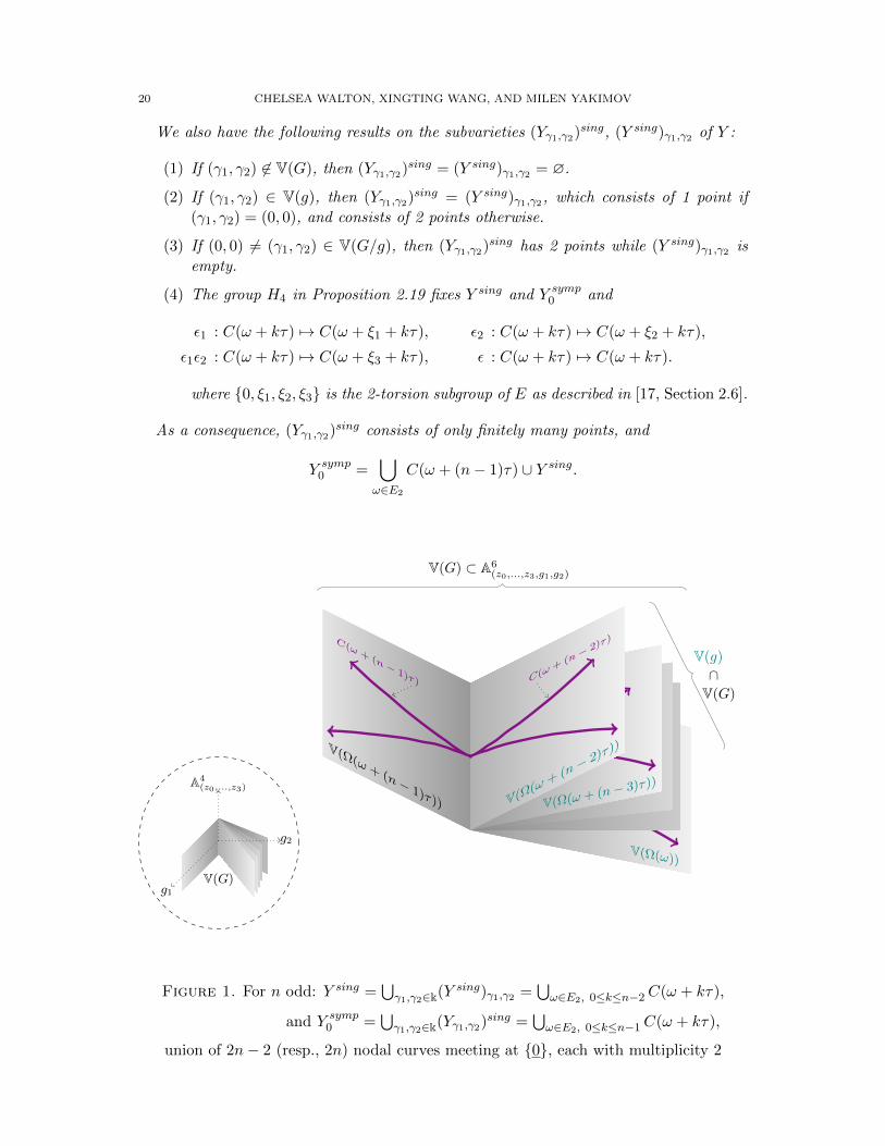
We also have the following results on the subvarieties (Yγ1,γ2)sing, (Y sing)γ1,γ2 of Y :

(1) If (γ1, γ2) 6∈ V(G), then (Yγ1,γ2)sing = (Y sing)γ1,γ2 = ∅.

(2) If (γ1, γ2) ∈ V(g), then (Yγ1,γ2)sing = (Y sing)γ1,γ2, which consists of 1 point if

(γ1, γ2) = (0, 0), and consists of 2 points otherwise.

(3) If (0, 0) 6= (γ1, γ2) ∈ V(G/g), then (Yγ1,γ2)sing has 2 points while (Y sing)γ1,γ2 is

empty.

(4) The group H4 in Proposition 2.19 fixes Y sing and Y symp0 and

ε1 : C(ω + kτ) 7→ C(ω + ξ1 + kτ), ε2 : C(ω + kτ) 7→ C(ω + ξ2 + kτ),

ε1ε2 : C(ω + kτ) 7→ C(ω + ξ3 + kτ), ε : C(ω + kτ) 7→ C(ω + kτ).

where 0, ξ1, ξ2, ξ3 is the 2-torsion subgroup of E as described in [17, Section 2.6].

As a consequence, (Yγ1,γ2)sing consists of only finitely many points, and

Y symp0 =

⋃ω∈E2

C(ω + (n− 1)τ) ∪ Y sing.

V(Ω(ω +(n−

1)τ))

C(ω+

(n−1)τ)

V(Ω(ω))

V(G) ⊂ A6(z0,...,z3,g1,g2)

V(g)

∩V(G)

V(Ω(ω + (n− 3)τ))

V(Ω(ω

+(n

− 2)τ))

C(ω+

(n− 2)

τ)

V(G)g1

g2

A4(z0,...,z3)

Figure 1. For n odd: Y sing =⋃γ1,γ2∈k(Y sing)γ1,γ2 =

⋃ω∈E2, 0≤k≤n−2C(ω + kτ),

and Y symp0 =

⋃γ1,γ2∈k(Yγ1,γ2)sing =

⋃ω∈E2, 0≤k≤n−1C(ω + kτ),

union of 2n− 2 (resp., 2n) nodal curves meeting at 0, each with multiplicity 2


Proof of Theorem 3.13. The Jacobian matrix of Y = V(π(p), π(q)) is∂fp∂z0

∂fp∂z1

∂fp∂z2

∂fp∂z3

∂hp∂g1

∂hp∂g2

∂fq∂z0

∂fq∂z1

∂fq∂z2

∂fq∂z3

∂hq∂g1

∂hq∂g2

.It is clear that if it has rank ≤ 1 at some point P = (P, γ1, γ2) ∈ Y , then the Jacobian

matrix of Yγ1,γ2 , which is one of its 2× 4 minors containing all the partial derivatives of

zi, also has rank ≤ 1 at P . So

(3.14) (Y sing)γ1,γ2 ⊆ (Yγ1,γ2)sing.

Now if P ∈ Y sing then each 2 × 2 minors of the matrix above vanishes at P . In

particular, we have that

det

∂hp∂g1

∂hp∂g2

∂hq∂g1

∂hq∂g2

(P ) = det

(∂(hp, hq)

∂(g1, g2)

)(γ1, γ2) = 0.

Hence Y sing ⊂ V(g) by Lemma 3.10 and

Y sing =⋃

(γ1,γ2)∈V(g)

(Y sing)γ1,γ2 ⊆⋃

(γ1,γ2)∈V(g)

(Yγ1,γ2)sing =⋃ω∈E2

0≤k≤n−2

C(ω + kτ)

by Lemma 3.12.

Conversely, we verify that C(ω + kτ) ⊂ Y sing for all ω ∈ E2 and 0 ≤ k ≤ n − 2 as

follows. Let π(ω) and π(q) be the two defining relations of Y with q ∈ E generic. It

suffices to show that the first row of the Jacobian matrix of Y above vanishes, i.e., we

want to show that[∂fω∂z0

, ∂fω∂z1, ∂fω∂z2

, ∂fω∂z3, ∂hω∂g1

, ∂hω∂g2

](tneω + t2pω,k)

= t2n[∂fω∂z0

(eω), ∂fω∂z1(eω), ∂fω∂z2

(eω), ∂fω∂z3(eω), 0, 0

]+ t2n

[0, 0, 0, 0, ∂hω∂g1

(pωk),∂hω∂g2

(pωk)]

vanishes. Since eω is the singularity of Q(ω), the first summand vanishes. Note that

when 0 ≤ k ≤ n− 2 we have pω,k ∈ Ω(ω + kτ) = Ω(ω + (n− 2− k)τ) is a multiple root

of hω =∏n−1k=0 Ω(ω + kτ). So, the second summand vanishes as well. Thus, the first part

of the result holds.

(1) This follows from Lemma 3.11.

(2) Suppose (γ1, γ2) ∈ V(g). By Lemma 3.12 and the beginning of the result, we have

that

(Y sing)γ1,γ2 = (Yγ1,γ2)sing = C(ω + kτ) ∩ V(g1 − γ1, g2 − γ2)

for some (γ1, γ2) ∈ V(Ω(ω + kτ)) with 0 ≤ k ≤ n − 2. If (γ1, γ2) = (0, 0), then

(Y sing)γ1,γ2 = (Yγ1,γ2)sing = (0, 0, 0, 0). If (γ1, γ2) 6= (0, 0), then since n is odd there

are two choices of t satisfying the defining equation of C(ω + kτ) yielding two different

points in (Y sing)γ1,γ2 = (Yγ1,γ2)sing.

(3) The argument for (Yγ1,γ2)sing is similar as in (2) noting that⋃(γ1,γ2)∈V(Ω(ω+(n−1)τ))

(Yγ1,γ2)sing = tneω + t2pω,n−1 | t ∈ k

for any ω ∈ E2 by Lemma 3.12.


For (Y sing)γ1,γ2 , recall from Notation 3.9 that G/g =∏ω∈E2

Ω(ω + (n − 1)τ). Since

g =∏ω∈E2,0≤k≤n−2 Ω(ω + kτ), we can see that G/g and g as polynomials in k[g1, g2]

have no common factors by using the only non-trivial identity (3.3) between these central

annihilators Ω(ω + kτ). By the argument in the beginning of the proof of this theorem,

we know Y sing ⊆ V(g). This implies that

(Y sing)γ1,γ2 = Y sing ∩ V(g1 − γ1, g2 − γ2) ⊂ V(g) ∩ V(g1 − γ1, g2 − γ2).

By the assumption on (γ1, γ2), we get V(g) ∩ V(g1 − γ1, g2 − γ2) = ∅ as gcd(G/g, g) = 1

in k[g1, g2]. Therefore, we have (Y sing)γ1,γ2 = ∅ if (0, 0) 6= (γ1, γ2) ∈ V(G/g).

(4) By Corollary 2.21(4) the group H4 ⊂ Autgr(S) fixes Y sing and Y symp0 . By [17,

Corollary 2.10], we know εi(Ω(ω+kτ)) = Ω(ω+ξi+kτ) for i = 1, 2. Note that C(ω+kτ) ⊂V(Ω(ω+kτ)). So we have εi(C(ω+kτ)) and C(ω+ξi+kτ) are included in V(Ω(ω+ξi+kτ)).

By Lemma 3.12, V(Ω(ω + ξi + kτ)) ∩ Y symp0 contains only one nodal curve, namely

tneω+ξi + t2pω+ξi,k | t ∈ k. So all three nodal curves are the same. Finally, ε is just a

rescaling of the variables of S. So it will fix all the nodal curves C(ω + kτ). This proves

part (4).

Finally, we have

Y symp0 = Y symp

0 ∩ V(G)

= (Y symp0 ∩ V(G/g)) ∪ (Y symp

0 ∩ V(g))

=⋃ω∈E2

C(ω + (n− 1)τ) ∪ Y sing.

So, the result follows.

3.2. For PIdeg(S) even. We now assume in this part that the PI degree n of S is even;

here, s = n/2 and ui = z2i with deg ui = s for all 0 ≤ i ≤ 3. Recall that the center of the

Veronese subalgebra S(2) is

Z(S(2)) = k[u0, u1, u2, u3](n)[g1, g2]

subject to two defining relations π(p) = fp + hp and π(q) = fq + hq, where the points

p, q ∈ E = E/〈σ2〉 satisfy p 6= ±q. Note that fp and fq are two linearly independent

quadrics in terms of u0, u1, u2, u3 defining the elliptic curve E ⊂ P. The center Z of S

isomorphic to k[z0, z1, z2, z3, g1, g2] subject to two defining relations F1, F2 of degree 2n.

Moreover, we can write the two defining relations of Z as

F1 = (a1 − h1)2 − zizj , F2 = (a2 − h2)2 − zkzl, i, j, k, l = 0, 1, 2, 3,

where h1, h2 ∈ k[g1, g2]n have no common factors and a1, a2 are linear forms in terms of

z0, z1, z2, z3 given in Proposition 2.23.

Lemma 3.15. For each pair (γ1, γ2) ∈ k2, we have that (Yγ1,γ2)sing ⊂ V(z0z1z2z3).

Proof. By way of contradiction, suppose there exists a point

P = (P, γ1, γ2) ∈ (Yγ1,γ2)sing \ V(z0z1z2z3)

for some γ1, γ2 ∈ k. Let mP

be the maximal ideal of Z(S) corresponding to P . Then by the

Lying Over Theorem (for the integral extension Z(S) ⊂ Z(S(2))), there exists a maximal

ideal n of Z(S(2)) so that n ∩ Z(S) = mP

. Moreover, V(n) is a point Q = (Q, γ1, γ2) of

maxSpec(Z(S(2))).


Using the fact that zi = u2i for all 0 ≤ i ≤ 3, we get Q 6∈ V(u0u1u2u3) since P is not in

V(z0z1z2z3). In particular, we have Q 6= 0. Moreover, since P ∈ (Yγ1,γ2)sing, we have that

Q is a singular point of maxSpec(Z(S(2)))∩V(g1 − γ1, g2 − γ2) via the Implicit Function

Theorem. Note that the defining relations of Z(S(2)) are of the same form as the defining

relations of Z(S) in the case when n is odd, we obtain by the argument in the proof of

Lemma 3.11 that the point Q is the singular point of some quadric containing E, namely

ek for some k = 0, . . . , 3. This contradicts Q 6∈ V(u0u1u2u3); see (3.7).

Theorem 3.16. [Y sing1 , Y sing

2 ] Take n even and recall the notation of Proposition 2.23.

Then, we obtain that the singular locus Y sing of Y = V(F1, F2) ⊂ A6(z0,z1,z2,z3,g1,g2) is the

union of subvarieties Y sing1 and Y sing

2 of Y defined by

(i) Y sing1 = V(a1 − h1, z0, z3) ∩ Y and Y sing

2 = V(a2 − h2, z1, z2) ∩ Y , when ρ = ρ1,

(ii) Y sing1 = V(a1 − h1, z0, z2) ∩ Y and Y sing

2 = V(a2 − h2, z1, z3) ∩ Y , when ρ = ρ2,

(iii) Y sing1 = V(a1 − h1, z0, z1) ∩ Y and Y sing

2 = V(a2 − h2, z2, z3) ∩ Y , when ρ = ρ3.

Moreover, we have Y sing1 ∩ Y sing

2 = 0.We also have the following results on the subvarieties (Yγ1,γ2)sing, (Y sing)γ1,γ2 of Y :

(1) The varieties Y sing1 and Y sing

2 from Theorem 3.16 are

permuted by

ε1 and ε2,

ε1 and ε1ε2,

ε2 and ε1ε2,

and fixed by

ε1ε2, when ρ = ρ1,

ε2, when ρ = ρ2,

ε1, when ρ = ρ3.

where εi are the group actions in Proposition 2.19.

(2) (Y sing)γ1,γ2 has 4 points generically (counting multiplicity), and 1 point if and

only if (γ1, γ2) = (0, 0).

(3) (Yγ1,γ2)sing = (Y sing)γ1,γ2 = (Y1)singγ1,γ2 ∪ (Y2)singγ1,γ2, where

(Yi)singγ1,γ2 := Y sing

i ∩ V(g1 − γ1, g2 − γ2)

for i = 1, 2.


g1

g2

• At (γ1, γ2) = (0, 0)

••

••

At (γ1, γ2) 6= (0, 0)

A2(z1,z2,γ1,γ2)

Y sing1

A2(z0,z3,γ1,γ2)

Y sing2 ••

••

At (γ′1, γ′2) 6= (γ1, γ2)

A2(z1,z2,γ′1,γ

′2)

Y sing1

A2(z0,z3,γ′1,γ

′2)

Y sing2

.

Figure 2. For n even with ρ = ρ1: Y sing = Y symp0 , union of surfaces Y sing

1 and Y sing2

Proof of Theorem 3.16. We will only treat the case for ρ = ρ1, and other cases are similar.

We use the presentation of Z in Proposition 2.23, where we can write the two defining

relations of Y as

F1 = (a1 − h1)2 − z0z3, F2 = (a2 − h2)2 − z1z2.

Moreover, we can assume that h1, h2 ∈ k[g1, g2]n have no common factors and

a1 = λ(z0 + asbsξ3nz3) + µ(z1 + asb−sξnz2)

a2 = µ(b−sc−nξ2nz0 + asc−nξ3nz3) + λ(bsz1 + asξ3nz2),

where λ, µ ∈ k with µ 6= 0 by Proposition 2.23.

Next, it is clear that (Y sing)γ1,γ2 ⊆ (Yγ1,γ2)sing ⊂ V(z0z1z2z3) using Lemma 3.15 for

the latter. We now show that Y sing is contained in the union of Y sing1 and Y sing

2 . Take

a point P = (P, γ1, γ2) ∈ (Y sing)γ1,γ2 , where P = (p0, . . . , p3). Then without loss of

generality, we can take p0 = 0 and hence a1 − h1 = 0 at P in Y sing. Now, let

A := a2 − h2

and consider the following Jacobian matrix (it has rank ≤ 1 at P )

∂(F1, F2)

∂(z0, . . . , z3, g1, g2)

∣∣∣a1=h1

=

[−z3 0 0 −z0 0 0

2A∂a2∂z0

2A∂a2∂z1− z2 2A∂a2

∂z2− z1 2A∂a2

∂z3−2A∂h2

∂g1−2A∂h2

∂g2

]

Recall that p0 = 0. Now if p3 = 0, then P is contained in Y sing1 . On the other hand,

suppose p3 6= 0. Then the determinant of the first two columns of the matrix above,

evaluated at P and set equal to 0, implies that

p2 = 2A∂a2

∂z1(P ).


Likewise, using the first and third columns, and also the first and fourth columns, respec-

tively, we get

p1 = 2A∂a2

∂z2(P ) and 2A

∂a2

∂z3(P ) = 0.

Since ∂a2∂z36= 0, we have that A = 0 and thus p1 = p2 = 0. Therefore, P ∈ Y sing

2 .

Conversely, it is straight-forward to check that Y sing1 and Y sing

2 are contained in Y sing.

So, Y sing = Y sing1 ∪ Y sing

2 .

Finally, let P = (p0, p1, p2, p3, γ1, γ2) ∈ Y sing1 ∩ Y sing

2 . Then we have pk = 0 for all k

(by Lemma 3.15) and (γ1, γ2) ∈ V(h1, h2). Since h1, h2 have no common factors, we get

γ1 = γ2 = 0 and P = 0, as desired.

(1) follows from Corollary 2.24.

(2) First, assume that (γ1, γ2) = (0, 0). Then (Y sing)0,0 ⊆ (Y0,0)sing, where Y0,0 =

k[z0, z1, z2, z3]/(Φ1,Φ2) is the affine cone of the smooth elliptic curve E′′ = E/〈σ〉 (see

Lemma 2.14). So we get (Y sing)0,0 = (Y0,0)sing = 0.Now suppose (γ1, γ2) 6= (0, 0) and ρ = ρ1. By the beginning of the statement, we have

Y sing1 = V(a1 − h1, z0, z3, (a2 − h2)2 − z1z2). So (Y sing

1 )γ1,γ2 is the intersection points

of a line a1 = h1 with a conic (a2 − h2)2 = z1z2 in the affine space A2(z1,z2,g1=γ1,g2=γ2),

which has two points (counting multiplicity). The same argument applies to (Y sing2 )γ1,γ2

as well. Since Y sing1 ∩ Y sing

2 = 0 by the beginning of the statement, we get that

(Y sing)γ1,γ2 = (Y sing1 )γ1,γ2 ∪ (Y sing

2 )γ1,γ2 has 4 points generically.

The argument for ρ = ρ2, ρ3 follows similarly.

(3) Recall that (Yγ1,γ2)sing ⊂ V(z0z1z2z3) by Lemma 3.15. Then, without loss of

generality take ρ = ρ1, and take z0 = 0 so that a1 = h1(γ), and consider the Jacobian

matrix of Yγ1,γ2

∂(F1(z, γ), F2(z, γ))

∂(z0, z1, z2, z3)

∣∣∣z0=0,a1=h1

=

[−z3 0 0 0

2A∂a2∂z0

2A∂a2∂z1− z2 2A∂a2

∂z2− z1 2A∂a2

∂z3

]where A = a2−h2(γ). With this matrix, we can show (Yγ1,γ2)sing ⊆ (Y1)singγ1,γ2 ∪ (Y2)singγ1,γ2 .

Moreover, we can conclude that

(Y1)singγ1,γ2 ∪ (Y2)singγ1,γ2 = (Y sing)γ1,γ2 ⊆ (Yγ1,γ2)sing ⊆ (Y1)singγ1,γ2 ∪ (Y2)singγ1,γ2 .

This proves the result.

4. Background material on Poisson orders and specialization

We discuss briefly in this section background material on Poisson orders, including the

process of specialization mentioned in the introduction, as well as material on symplectic

cores. More details can be found in [43, Sections 2.1 and 2.2] and the references therein.

4.1. Poisson orders and specialization. Here we collect some definitions and facts

about Poisson orders and describe an extension of the specialization technique for ob-

taining such structures. The following definition is due to Brown and Gordon [13].

Definition 4.1. [Der(A/C), ∂, ∂z] Let A be a k-algebra which is module-finite over a

central subalgebra C. Denote by Der(A/C) the algebra of k-derivations of A that preserve

C.


The algebra A is called a Poisson C-order if there exists a k-linear map

∂ : C → Der(A/C)

such that the induced bracket ., . on C given by

(4.2) z, z′ := ∂z(z′), z, z′ ∈ C

makes C a Poisson algebra. The triple (A,C, ∂ : C → Der(A/C)) will be also called a

Poisson order in places where the role of ∂ needs to be emphasized.

As discussed in [13, Section 2.2], specializations of families of algebras give rise to

Poisson orders. In our previous work [43] we generalized this construction to obtain

Poisson orders from higher degree terms in the derivation ∂; this is reviewed as follows.

Definition 4.3. Let R be an algebra over k and ~ be a central element of R which

is regular, i.e., not a zero-divisor of R. We refer to the k-algebra R0 := R/~R as the

specialization of R at ~ ∈ Z(R).

Notation 4.4. [θ, ι, N ] Retain the notation of Definition 4.3. Let [-, -] denote the com-

mutator of elements of R. Let θ : R R0 be the canonical projection; so, ker θ = ~R.

Fix a linear map ι : Z(R0) → R such that θ ι = idZ(R0). Let N ∈ Z+ be such that

(4.5) [ι(z), y] ∈ ~NR for all z ∈ Z(R0), y ∈ R.Note that (4.5) holds for N = 1: take y ∈ θ−1(y) for y ∈ R0 and we get θ([ι(z), y]) =

[z, y] = 0; further, ker θ = ~R.

Definition 4.6. Retain the notation above. For y ∈ R0 and z ∈ Z(R0), the special

derivation of level N is defined (in fact, well-defined) as

(4.7) ∂z(y) := θ

([ι(z), y]

~N

), where y ∈ θ−1(y).

The next result states that ∂z is indeed a derivation, and thus specializations yield

Poisson orders.

Proposition 4.8. [43, Proposition 2.7 and Corollary 2.8] Let R be a k-algebra and ~ ∈Z(R) be a regular element. Assume that ι : R0 := R/(~R) → R is a linear section of the

specialization map θ : R R0 such that (4.5) holds for some N ∈ Z+. Assume that R0

is module-finite over Z(R0).

(1) If, for all z ∈ Z(R0), ∂z is a special derivation of level N , then

(R0, Z(R0), ∂ : Z(R0)→ Der(R0/Z(R0)))

is a Poisson order and the map ∂ is a homomorphism of Lie algebras.

(2) If C ⊂ Z(R0) is a Poisson subalgebra of Z(R0) with respect to the Poisson struc-

ture (4.2) and R0 is module-finite over C, then R0 is a Poisson C-order via the

restriction of ∂ to C.

(3) If, in addition to (2), the restricted section ι : C → R is an algebra homomor-

phism, then

∂zz′(y) = z∂z′(y) + z′∂z(y) for z, z′ ∈ C, y ∈ R0.

We coined such a construction with the following terminology.

Definition 4.9. [43, Definition 2.9] The Poisson order produced in Proposition 4.8 is a

Poisson order of level N when the level of the special derivation needs to be emphasized.


4.2. Symplectic cores and the Brown-Gordon theorem. Poisson orders can be used

to establish isomorphisms for different central quotients of a PI algebra via the result of

Brown and Gordon [13] provided below. The result relies on the notion of symplectic

core, introduced in [13]. We recall some terminology from [13, Section 3.2].

Definition 4.10. [P(I)] Let (C, ., .) be an affine Poisson algebra over a field k of

characteristic 0. For every ideal I of C, there exists a unique maximal Poisson ideal

contained in I, to be denoted by P(I). If I is prime, then P(I) is Poisson prime, [25,

Lemma 6.2].

(1) We refer to P(I) above as the Poisson core of I.

(2) We say that two maximal ideals m, n ∈ maxSpecC of an affine Poisson algebra

(C, ., .) are equivalent if P(m) = P(n).

(3) The equivalence class of m ∈ maxSpecC is referred to as the symplectic core of

m. The corresponding partition of maxSpecC is called symplectic core partition.

One main benefit of using the symplectic core partition is the powerful result below.

Theorem 4.11. [13, Theorem 4.2] Assume that k = C and that A is a Poisson C-order

which is an affine C-algebra. If m, n ∈ maxSpecC are in the same symplectic core, then

there is an isomorphism between the corresponding finite-dimensional C-algebras

A/(mA) ∼= A/(nA).

5. A specialization setting for 4-dimensional Sklyanin algebras

The goal of this section is to produce a setting so that the PI 4-dimensional Sklyanin

algebras arise as Poisson orders via specialization; see Section 4.1. The section also sets

up some of the notation regarding Poisson orders that we will use throughout this work.

Recall that S := S(α, β, γ) is a 4-dimensional Sklyanin algebra and we do not nec-

essarily need that S is module-finite over its center Z. In any case, recall that B (∼=S/(Sg1 + Sg2)) is the corresponding twisted homogeneous coordinate ring.

The reader may wish to view Figure 3 at this point for a preview of the setting that

we will construct for S. Our objective is to produce a degree 0 deformation S~ of S

using a formal parameter ~. The specialization map for S will be realized via a canonical

projection θS : S~ → S given by ~ 7→ 0. Moreover, S~ will have the structure of a

k[[~]]-algebra.

Notation 5.1. [~, α, β, γ] To begin, we fix a formal parameter ~ and let

α := α+ α1~ + α2~2 + · · · , β := β + β1~ + β2~2 + · · · , γ := γ + γ1~ + γ2~2 + · · · ,

in k[[~]] satisfying α+ β + γ + αβγ = 0 (a version of (2.2)).

It is clear that a version of (2.3) holds for the formal parameters α, β, γ as well.

Definition 5.2. [S~, S~] Denote by S~ the 4-dimensional Sklyanin algebra over k((~))

with parameters (α, β, γ). Define the formal Sklyanin algebra to be the k[[~]]-subalgebra

S~ of S~ generated by x0, x1, x2, x3, that is,

S~ := k[[~]]〈x0, x1, x2, x3〉 ⊂ S~.


It is important to point out that S~ is a graded k[[~]]-algebra with the grading inherited

from S~ such that deg(~) = 0 and deg(xi) = 1 for 0 ≤ i ≤ 3. Recall by Lemma 2.9 we

obtain the following result.

Lemma 5.3. [g1, g2] The elements

g1 = −x20 + x2

1 + x22 + x2

3 and g2 = x21 + (1 + α)(1− β)−1x2

2 + (1− α)(1 + γ)−1x23

form a central regular sequence in S~.

Lemma 5.4. The following statements hold for the formal Sklyanin algebra S~.

(1) S~ ∼= k((~))⊗k[[~]] S~.

(2) At each degree d of S~, we get that (S~)d is a free k[~]]-module of rank(d+3

3

).

(3) The elements g1, g2 belong to the center of S~.

(4) There is a natural surjection from S~ S via ~ 7→ 0 with kernel equal to ~S~.

Proof. (1) This is clear from the definitions of S~ and S~.

(2) Since S~ is a domain, each graded piece (S~)d ⊂ (S~)d is a finitely generated

torsion-free module over k[[~]]. Because k[[~]] is a PID, this implies that (S~)d is a free

k[[~]]-module. By (1), (S~)d has rank equal to dim(S~)d, which in turn is equal to(d+3

3

)for S~ has Hilbert series 1/(1− t)4.

(3) It is easy to check that g1, g2 ∈ Z(S~) ∩ S~ ⊂ Z(S~).

(4) It suffices to show that S~/~S~ ∼= S. Clearly there is a surjection S S~/~S~.

Moreover, it is an isomorphism since on each degree dimSd = dim(S~)d/~(S~)d =(d+3

3

)by (2). The kernel part follows directly.

Notation 5.5. [θS ] Denote by θS the corresponding specialization map for the formal

Sklyanin algebra S~, namely

θS : S~ → S given by ~ 7→ 0.

So, the first column in Figure 3 below is established and we now turn our attention to

the second column of that figure.

Definition 5.6. [E~, L~, σ~, B~, B~] Denote by E~ the elliptic curve over k((~)), by L~ =

OP3(1)|E~ the invertible sheaf over E~, and by σ~ the automorphism of E~ corresponding

to S~ as in Definition-Lemma 2.4 with (α, β, γ) replaced by (α, β, γ) from Notation 5.1.

Let

B~ := B(E~,L~, σ~)

be the corresponding twisted homogeneous coordinate ring. Its k[[~]]-subalgebra

B~ := k[[~]]〈x0, x1, x2, x3〉 ⊂ B~,

generated by x0, x1, x2, x3, will be called formal twisted homogeneous coordinate ring.

Lemma 5.7. [ψ~] The canonical projection S~ B~ induces a surjection ψ~ : S~ B~,

whose kernel is generated by g1, g2. As a consequence, the composition S~θS S B

factors through the map ψ~.


Proof. Note that ψ~ is the composition S~ → S~ B~, whose image is B~ by definition.

So it remains to show

ker(ψ~) = (g1S~ + g2S~) ∩ S~ = g1S~ + g2S~.

For simplicity, we write M := g1S~ and N := g1S~ ∩ S~. It is clear that M ⊆ N , which

are both graded ideals in S~. By Lemma 5.4(1), we have M ⊗k[[~]] k((~)) = N . Hence,

as finitely generated free modules over k[[~]], we get that rank(Md) = rank(Nd) in each

degree d. So (N/M)d is a torsion module over k[[~]]. Then for any r ∈ Nd, there exists

an integer m such that ~mr = yg1 for some y ∈ (S~)d−2. Since ~ - g1, we get that ~d | yand r ∈ Md. This implies Md = Nd for every d, and M = N . By a similar argument,

we can then conclude that (g1S~ + g2S~) ∩ S~ = g1S~ + g2S~ where the left-hand side is

equal to ker(ψ~). Finally, the factorization through ψ~ is straight-forward.

Definition 5.8. [θB] Let θB : B~ B be the map induced by Lemma 5.7, which we call

the specialization map for the formal twisted homogeneous coordinate ring B~.

Now we complete the verification of Figure 3 as follows.

Definition 5.9. [w, L~, v′0, v′1, v′2, v′3, R~] Fix a nonzero section w ∈ H0(E,L), which is

also realized as an element of H0(E~,L~) via the vector space isomorphism H0(E~,L~) ∼=k((~)) ⊗k H

0(E,L). Denote by L~ the k[[~]]-subalgebra of the function field k((~))(E~)

generated by v′0 := v0/w, v′1 := v1/w, v′2 := v2/w and v′3 = v3/w satisfying the dehomog-

enized relations:

φ1(v′0, v′1, v′2, v′3) = v′20 + v′21 + v′22 + v′23 = 0

φ2(v′0, v′1, v′2, v′3) = (1− γ)(1 + α)−1v′21 + (1 + γ)(1− β)−1v′22 + v′23 = 0.

We call R~ := (L~)(~) the integral form of the field k((~))(E~).

Note that the quotient field of L~ is Q(L~) ∼= k((~))(E~). Using (2.5) with replacing

(α, β, γ) by (α, β, γ), one sees that the automorphism σ~ ∈ Aut(k((~))(E~)

)restricts to

an automorphism of R~, given by

σ~(v′i) = σ~(vi/w) =σ~(vi)/w

2

σ~(w)/w2, for all 0 ≤ i ≤ 3.

Let D and D~ be the divisors of zeros of w for E and E~, respectively. In view of

Lemma 2.8, we have the following commutative diagram.

(B~)1 = H0(E~,L~)∼= // H0(E~,O(D~))t

// k((~))(E~)[t±1;σ~]

(B~)1 = k[[~]]⊗k H0(E,L)

∼= //?

OO

~ 7→0

k[[~]]⊗k H0(E,O(D~))t

//?

OO

~ 7→0

R~[t±1;σ~]?

OO

~ 7→0

B1 = H0(E,L)∼= // H0(E,O(D))t

// k(E)[t±1;σ]

Moreover, we have the canonical embeddings

(5.10) B~ → R~[t±1;σ~] → k((~))(E~)[t±1;σ~].

The ring R~[t±1;σ~] is a graded localization of B~ by an Ore set which does not intersect

the kernel ker θB = ~B~. Therefore, the following map is well-defined.


Definition 5.11. [θR] Let θR : R~[t±1;σ~] k(E)[t±1, σ] be defined by

θR(v′i) = v′i, for all 0 ≤ i ≤ 3, θR(t) = t, θR(~) = 0,

which is the extension of θB via localization. We also denote by θR its restriction to the

specialization map R~ k(E). These maps are referred to as the specialization maps for

the integral form of the formal twisted homogeneous coordinate B.

The commutativity of the cells in Figure 3 between the second and third column follows

directly from the definitions of the maps within this part of the diagram and from the

previous commutative diagram.

S~ = S(α, β, γ)mod(g1,g2) // // B~ = B(E~,L~, σ~)

gr. quot. ring // k((~))(E~)[ t±1;σ~]

S~ = k[[~]]〈x0, x1, x2, x3〉mod(g1,g2) // //

?

OO

θS

B~ = k[[~]]〈x0, x1, x2, x3〉 //

?

OO

θB

R~[ t±1;σ~]?

OO

θR

S = S(α, β, γ)

mod(g1,g2) // // B = B(E,L, σ) gr. quot. ring // k(E)[ t±1;σ]

Z (S)mod(g1,g2) // //

?

OO

Z(B)?

OO

gr. quot. ring // k(E)σ[ t±n;σ]?

OO

Figure 3. Specialization setting for Sklyanin algebras:

integral forms, Poisson orders, and centers are respectively in the last three rows.

6. Poisson orders on PI 4-dimensional Sklyanin algebras S

This section establishes a construction of Poisson orders on PI 4-dimensional Sklyanin

algebras with the property that the induced Poisson structure on its center is nontrivial.

Recall that S is a PI 4-dimensional Sklyanin algebra of PI degree n = |σ| corresponding

to the parameters α, β, γ ∈ k satisfying (2.2) and (2.3). Let the scalars αi, βi, γi defining

α, β, γ in Notation 5.1, for i ≥ 1, be such that

(6.1) α+ β + γ + αβγ = 0 and |σ~| =∞.

Such scalars exist because (α, β, γ) ∈ A3 | |σαβγ | = n is a closed subset of the surface

V(α+ β + γ + αβγ) ⊂ A3.

6.1. Construction of Poisson orders. Throughout the section we will identify the first

graded pieces S1 of S and B1 of B with each other through vector space isomorphism

(Lemma 2.9). In particular, x0, x1, x2, x3 is a good basis of B1 as in Lemma 2.17.

Notation 6.2. [xi, zi] Denote by xi the preimage of xi under the specialization map

θS : S~ S which is given by the same linear combinations of the standard generators


of S~ as is xi given in terms of the standard generators of S. Moreover, set

zi := xni +∑

1≤j<n/2 cij gj xn−2ji ∈ S~, 0 ≤ i ≤ 3

for the polynomials cij ∈ k[g1, g2]2j from Proposition 2.18(1).

Definition 6.3. Consider the terminology below.

(1) A degree 0 section ι : Z → S~ of the map θS : S~ S will be called good if

(i) ι(zi)− zi ∈ g1k[xi, g1, g2, ~] + g2k[xi, g1, g2, ~], and

(ii) ι(g1) = g1 and ι(g2) = g2.

(2) A specialization map θS : S~ → S will be called a good specialization of S of

level N if there exists a good section ι : Z → S~ such that

(6.4) [ι(z), y] ∈ ~NS~ for all z ∈ Z, y ∈ S~.

Given any section ι : Z → S~ of θS ,

[ι(z), y] ∈ ~S~ for all z ∈ Z, y ∈ S~.

Therefore, N ≥ 1. Next, we prove that for a given PI 4-dimensional Sklyanin algebra S,

the levels N of good specializations for S are bounded from above.

Lemma 6.5. Let S be a PI Sklyanin algebra corresponding to the parameters α, β, γ ∈ ksatisfying (2.2) and (2.3) and there exist formal parameters α, β, γ satisfying (6.1).

Then, the set of levels N for good sections of θS has an upper bound.

Proof. Consider the algebras L~ and R~ := (L~)(~) from Definition 5.9 for w = x0,

identified as the preimage of v′0 under θB. Since the condition (6.1) is satisfied, the

automorphism σ~ of R~ has infinite order. This gives

(6.6) Rσn~~ ( R~.

On the other hand, ~ ∈ R~ is a regular element, from which one gets

(6.7)⋂l∈Z+

~lR~ = 0.

Combining (6.6) and (6.7), we obtain that there exists a positive integer M such that

(6.8) rσn~ − r /∈ ~MR~ for some r ∈ R~.

Denote by Mmin the least such positive integer, and by rmin ∈ R~ an element satisfy-

ing (6.8) for this integer Mmin. Although, it will not play a role in the proof, we note

that Mmin ≥ 2 because rσn~ − r ∈ ~R~ for all r ∈ R~.

In the remainder of the proof, we will show that

N < Mmin

which gives the stated upper bound for levels of good sections. Let ι : Z → S~ be one

such good section of θS , with respect to which the specialization map θS has level N .

Recall the map ψ~ : S~ B~ from Lemma 5.7. Then, the condition (6.4) implies that

[ψ~ι(z), y] ∈ ~NB~, ∀ z ∈ Z, y ∈ B~.

From (5.10) we have B~ → R~[t±1;σ~] with respect to which R~[t±1;σ~] is a localization

of B~. Hence,

(6.9) [ψ~ι(z), y] ∈ ~NR~[t±1;σ~], ∀ z ∈ Z, y ∈ R~[t±1;σ~].


Proposition 2.18, combined with the facts that kerψ~ = g1S~ + g2S~ (from Lemma 5.7)

and that ι is a good section, leads to ψ~ι(z1) = tn ∈ R~[t±1;σ~]. By applying (6.9) to

z = z1 and y = rmin ∈ R~, we obtain that

[tn, rmin] = (rσn~min − rmin)tn ∈ ~NR~[t±1;σh] for all r ∈ R~.

Since t is a unit of R~[t±1;σh],

rσn~min − rmin ∈ ~NR~.

The last equation implies that N < Mmin because rσn~min − rmin /∈ ~MminR~.

The main theorem of this section establishes the structure of Poisson order on each PI

4-dimensional Sklyanin algebra S for which the Poisson structure on the center of S is

nontrivial.

Theorem 6.10. Let S be a PI 4-dimensional Sklyanin algebra satisfying (2.2)–(2.3) as

above. Each Poisson order (S,Z, ∂ : Z → Der(S/Z)) of level N , coming from a good

specialization of maximum level N , has the property that the induced Poisson structure

on Z is non-zero.

One interesting direction for further investigation is as follows.

Question 6.11. Given PI 4-dimensional Sklyanin algebra S as used in Theorem 6.10,

what is the maximal level N of a good specialization for S?

One approach to this question is to determine the minimal positive integer Mmin from

the proof of Lemma 6.5 which is explicitly defined in (6.8) and then to use the upper

bound N ≤Mmin.

6.2. Derivations of PI S. We classify a certain type of derivations of S which will play

a role in the proof of Theorem 6.10. This description will be obtained in three stages

where similar types of derivations of the algebras in Notation 6.12 are classified.

In fact, the techniques below can be generalized easily to obtain similar results for PI

algebras T where some factor of T by a regular central sequence is the twisted homoge-

neous coordinate ring of an elliptic curve; see Theorem 6.19.

Notation 6.12. [S′, ψ, ψ1, ψ2] For S a PI 4-dimensional Sklyanin algebra of PI degree

n < ∞ with center Z := Z(S). Recall B = S/(g1S + g2S) and denote S′ := S/(g1S).

Moreover, denote the canonical projections

ψ1 : S → S′, ψ2 : S′ → B, and ψ := ψ2ψ1 : S → B.

So,

kerψ1 = g1S, kerψ2 = g2S′, and kerψ = g1S + g2S.

Lemma 6.13. In the notation above, we have

ψ1(Z) = Z(S′) and ψ2(Z(S′)) = Z(B).

Proof. Since ψ(Z) = Z(B),

ψ2(Z(S′)) = Z(B).

The map ψ1 is surjective, thus

(6.14) ψ1(Z) ⊆ Z(S′).


Both sides of the inclusion are N-graded algebras with

ψ1(Z) =⊕

k∈N ψ1(Zk), Z(S′) =⊕

k∈N Z(S′)k.

To prove that (6.14) is an equality, one needs to prove that

(6.15) ψ1(Zk) = Z(S′)k,

which we show by induction on k.

The equality is obvious for k = 0. Let k be a positive integer. Assume that (6.15)

holds for indices less than k. It follows from the equality ψ(Z) = Z(B) that for each

z′ ∈ Z(S′)k, there exists z ∈ Zk such that

z′ − ψ1(z) ∈ kerψ2 = g2S′.

Write z′ − ψ1(z) = g2u′ for some u′ ∈ S′k−2. The assumptions on z and z′ imply that

g2u′ ∈ Z(S′)k. Therefore, u′ ∈ Z(S′)k−2 because g2 is a regular central element of S′ of

degree 2. It follows from the induction assumption that u′ = ψ1(u) for some u ∈ Zk−2.

Finally, using that g2 ∈ Z2, we obtain

z + g2u ∈ Z(S)k and z′ = ψ1(z + g2u) ∈ ψ1(Zk),

which completes the induction and the proof of the lemma.

Notation 6.16. [adr] As usual, for an algebra R and r ∈ R, adr will denote the inner

derivation of R given by adr(r′) := [r, r′] = rr′ − r′r.

Proposition 6.17. [x, δ] Assume that S is a PI 4-dimensional Sklyanin algebra of PI

degree n = |σ| <∞. Let x ∈ S1∼= B1 be a good element.

(1) If δ ∈ DerB is such that

(i) δ|Z(B) = 0, (ii) δ(x) = 0, (iii) deg δ = l with l ≤ n,

then

δ =

0, if l ≤ 0 or l = n

λ adxl , if 0 < l < n.

for some λ ∈ k.

(2) If δ ∈ DerS′ is such that

(i) δ|Z(S′) = 0, (ii) δ(x) = 0, (iii) deg δ = l with l ≤ n,

then δ = adp′ for some p′ ∈ k[x, g2]l such that degx p′ < n.

(3) If δ ∈ DerS is such that

(i) δ|Z = 0, (ii) δ(x) = 0, (iii) deg δ = l with l ≤ n,

then δ = adp for some p ∈ k[x, g1, g2]l such that degx p < n.

Proof. (1) For l < n, the statement of this part of the proposition (even without the

assumption that δ|Z(B) = 0) was proved by Smith and Tate in [39, Theorem 3.3]. Suppose

that l = n. Recall that the graded quotient ring of B is identified with k(E)[t±1;σ] by

sending x 7→ t. The derivation δ ∈ Der(B) can be extended to a derivation of k(E)[t;σ],

to be denoted by the same symbol. The conditions (i)–(ii) give that

δ(t) = 0 and δ(k(E)σ) = 0.

Choose y ∈ k(E) and let q(t) ∈ k(E)σ be its minimal polynomial over k(E)σ. Since the

extension k(E)/k(E)σ is separable, q′(y) 6= 0. The assumption that deg δ = n implies


that δ(y) ∈ k(E)xn commutes with y. Therefore 0 = δ(q(y)) = δ(y)q′(y) and, hence,

δ(y) = 0. We have that δ(k(E)) = 0 and δ(t) = 0, so δ = 0.

(2) Since δ(g2) = 0, ψδ : S′ → B descends to a derivation of B, which will be denoted

by the same symbol.

We prove part (2) by induction on l. If l ≤ 0, then ψ2δ is a homogeneous derivation of

B such that

ψ2δ|Z(B) = 0, ψ2δ(x) = 0, and degψ2δ ≤ 0

because ψ2(Z(S′)) = Z(B) (see Lemma 2.14). Part (1) implies that ψ2δ = 0. Thus,

δ(S′1) ⊆ kerψ2 = g2S′ ⊆ S′≥2. On the other hand, it follows from deg δ ≤ 0 that

δ(S′1) ⊆ S′≤1.

This implies that δ(S′1) = 0 and, consequently that δ = 0 because S′ is generated in

degree 1.

Let 1 ≤ l ≤ n. Assume by way of induction that the statement of part (2) holds for

derivations of degree less than l. Let δ be a derivation of S′ of degree l ∈ [1, n] such that

δ|Z(S′) = 0 and δ(x) = 0. As explained earlier, ψ2δ : S′ → B descends to a derivation of

B which satisfies

ψ2δ|Z(B) = 0, ψ2δ(x) = 0, and degψ2δ = l ∈ [1, n]

because ψ2(Z(S′)) = Z(B). It follows from part (1) that

ψ2δ = λ adxl

for some λ ∈ k such that λ = 0 if l = n. Therefore,

im(δ − λ adxl) ⊆ S′g2.

Using that g2 is a regular element of S′, we define

δ− := 1g2

(δ − λ adxl) ∈ Der(S′).

The assumptions on δ imply at once that

δ−|Z(S′) = 0, δ−(x) = 0, and deg δ− = l − 2.

By the inductive assumption there exists h′ ∈ k[x, g2]l−2 such that δ− = adh′ , and

degx h′ < n. Therefore,

δ = adp′ for p′ := g2h′ + λxl ∈ k[x, g2]l.

Since λ = 0 if l = n, we have degx p′ < n. This completes the proof of part (2).

Part (3) is derived from part (2) in the same fashion as (2) is derived from (1) making

use of the fact that g1 is a regular element of S.

Now the techniques above yield the general statements about derivations of certain PI

algebras as follows.

Notation 6.18. [T , Ωk, T[k], ψk] Let T be a connected N-graded algebra, and Ω1, . . . ,Ωm

a regular central sequence of elements of T of positive degree. Let

T [k] := T/(Ω1T + · · ·+ ΩkT )

for all 1 ≤ k ≤ m so that T [0] := T . Note that T [k] ∼= T [k−1]/(ΩkT[k−1]) and let

ψk : T [k−1] T [k] be the canonical projection.


Observe that if T [k] is module-finite over its center, then so is T [i] for all i < k by [39,

Lemma 3.6].

Theorem 6.19. Retain the notation above. Then the following statements hold.

(1) ψk(Z(T [k−1])) = Z(T [k]) for all 1 ≤ k ≤ m.

(2) Suppose that T [m] is isomorphic to BT := B(ET ,LT , σT ), a twisted homogeneous

coordinate ring of an elliptic curve ET ⊂ Pd with LT = OPd(1)|ET and σT in

Aut(ET ) given by translation. Assume, further, that BT is module-finite over its

center so that |σT | <∞. Let xT be a good element of BT of degree 1.

If δ is a derivation of T [k] such that

(i) δ|Z(T [k]) = 0, (ii) δ(xT ) = 0, (iii) deg δ = l with l ≤ |σT |,

then δ = adp for some p ∈ k[xT ,Ωk+1, . . . ,Ωm]l such that degxT p < |σT |.

6.3. Proof of Theorem 6.10, nontriviality of Poisson order structure on S. Let

ι : Z → S~ be a good section of maximal level N . Let ∂ : Z → Der(S/Z) be the

corresponding Poisson order. We need to prove that the induced Poisson structure on

Z is nontrivial. By way of contradiction, assume that this is not the case. Then, for

0 ≤ i ≤ 3, we have

(i) ∂zi |Z = 0, (ii) ∂zi(xi) = 0, (iii) deg ∂zi = n.

Property (i) is a restatement of the vanishing of the Poisson structure. Property (ii)

follows from the definition of good section, and more precisely the condition in Defini-

tion 6.3(1.i) and Notation 6.2. Namely, we have [ι(zi), xi] = 0 and thus,

∂zi(xi) = θ([ι(zi), xi]/~N ) = 0.

The third condition is a consequence of the fact that ι(zi) ∈ (S~)n. It follows from

Proposition 6.17(3) that there exist polynomials pi for 0 ≤ i ≤ 3

(6.20) pi(xi, g1, g2) ∈ k[xi, g1, g2]n and degxi pi(xi, g1, g2) < n

such that ∂zi = adpi(xi,g1,g2). We modify the section ι : Z → S~ to form a new good

section ι∨ : Z → S~ by first setting

ι∨(g1) := g1, ι∨(g2) := g2 and ι∨(zi) := ι(zi)− ~Npi(xi, g1, g2)

for 0 ≤ i ≤ 3. Then we choose a k-basis of Z of the form

B := gm11 gm2

2 zl00 zl11 z

l22 z

l33 | (m1,m2, l0, l1, l2, l3) ∈ L

for some L ⊂ N6 and complete the definition of ι∨ by setting

(6.21) ι∨(gm1

1 gm22 zl00 z

l11 z

l22 z

l33

)= ι∨(g1)m1ι∨(g2)m2ι∨(z0)l0ι∨(z1)l1ι∨(z2)l2ι∨(z3)l3

for all (m1,m2, l0, l1, l2, l3) ∈ L.

The two properties of the polynomials pi in (6.20) imply that ι∨ : Z → S~ is a good

section of θS . Furthermore, we have that

(6.22) [ι∨(zi), y] ∈ ~N+1S~, ∀ 0 ≤ i ≤ 3, y ∈ S~.


This follows from the equalities

[ι∨(zi), y] = ~N(

[ι(zi), y]

~N+ [pi(xi, g1, g2), y]

),

θS

([ι(zi), y]

~N+ [pi(xi, g1, g2), y]

)= ∂zi(θ(y))− ∂zi(θ(y)) = 0

and the fact that ker θS = ~S~, proved in Lemma 5.4(4).

Combining (6.21) and (6.22), we obtain that

[ι∨(z), y] ∈ ~N+1S~, ∀z ∈ B, 0 ≤ i ≤ 3, y ∈ S~.

This is a contradiction, since N equals the maximum level of a good section of the

projection θS : S~ → S. The contradiction implies that the induced Poisson structure on

Z from the Poisson order ∂ is nontrivial.

7. The Jacobian structure of Poisson orders on PI 4-dimensional Sklyanin

algebras

The goal of this part is to describe the Jacobian structure of the (nontrivial) Poisson

bracket on the center of the PI 4-dimensional Sklyanin algebras that arise as a Poisson

order via good specialization of maximal level. We begin this section with a straight-

forward result about PI algebras that are Poisson orders via specialization.

Proposition 7.1. Recall Notation 6.18. For a formal parameter ~, suppose that there

exists an k[[~]]-algebra T~ which is an k[[~]]-torsionfree degree 0 deformation of T so that

T~/(~T~) ∼= T . Take θT : T~ T , the canonical projection, and let Ωk ∈ Z(T~) be a lift

of Ωk ∈ Z(T ) via θT for all 1 ≤ k ≤ m.

Then, for every specialization of T of level N equipped with a section ι : Z(T ) → T~with ι(Ωk) = Ωk for all 1 ≤ k ≤ m, we have that ∂Ωk = 0 for the corresponding Poisson

order on T . In particular, Ω1, . . . ,Ωm are in the Poisson center of Z(T ).

Proof. For y ∈ T and y ∈ θ−1T (y), we get that ∂Ωk(y) = θT

([Ωk, y]/~N

), which is equal

to 0. Therefore, ∂Ωk = 0, and the second statement holds by the definition of a Poisson

order.

Applying this to the PI 4-dimensional Sklyanin algebras S, we have the statement

below.

Corollary 7.2. The central elements g1, g2 lie in the Poisson center of Z = Z(S) when

S arises as a Poisson Z-order of level N via specialization.

Proof. Apply Proposition 7.1 by taking T = S, T~ = S~, Ω1, . . . ,Ωm = g1, g2 and by

using Lemma 5.4(3).

Next, we have a general result pertaining to the Poisson structure of the PI algebras

T from above.

Proposition 7.3. [J(F )k,l] Recall Notation 6.18 and we abuse some notation utilized

above as follows. Suppose that T is module-finite over its center with Z(T ) generated

by algebraically independent homogeneous elements z1, . . . , zd, along with homogenous

elements Ω1, . . . ,Ωm, subject to d− 2 homogeneous relations F1, . . . , Fd−2.


Suppose that Y := V(F1, . . . , Fd−2) ⊂ Ad+m is an irreducible affine variety and define

the Jacobian matrix to be

J(F )k,l := (−1)k+ldet

(∂(F1, F2, . . . , Fd−3, Fd−2)

∂(z1, . . . , zk, . . . , zl, . . . , zd)

), for k < l

and J(F )l,k = −J(F )k,l. Moreover, suppose that Z(T ) = k[Y ] admits a (homogeneous)

Poisson structure of degree 0 so that

(i) Ω1, . . . ,Ωm are in the Poisson center,

(ii) J(F )k,l 6= 0 for some 1 ≤ k, l ≤ d,

(iii)⋂

1≤k,l≤d k[Y ][(J(F )k,l)−1] = k[Y ], where the intersection is taken over J(F )k,l 6= 0.

Then, the Poisson bracket on Z(T ) is determined by Jacobian matrices above as follows:

(7.4) zk, zl = ηJ(F )k,l, for all 1 ≤ k, l ≤ d, and for some η ∈ k[Y ].

If, further, η has degree 0, then η ∈ k[Y ]0 = k.

Proof. By condition (i) we have that

zk, Fi =

d∑l=1

zk, zl∂Fi/∂zl +

m∑l=1

zk,Ωl∂Fi/∂Ωl =

d∑l=1

zk, zl∂Fi/∂zl = 0.

Now consider the vector space of all (d− 1)-tuples over the base field k(Y ), which is the

fraction field of the domain k[Y ] by assumption. Note that the vector

V = (zk, z1, . . . , zk, zk, . . . , zk, zd)

is perpendicular to vectors (∂Fi/∂z1, . . . , ∂Fi/∂zk, . . . , ∂Fi/∂zd) for all 1 ≤ i ≤ d− 2. By

condition (ii) and Cramer’s rule, we know V has to be proportional to the vector

(J(F )k,1, . . . , J(F )k,k−1, J(F )k,k+1, . . . , J(F )k,d) .

So we can write

zk, zl = ηklJ(F )k,l, for some ηkl ∈ k(Y ).

By construction, we get ηkl = ηkl′ and ηkl = ηlk. Hence, ηkl = η ∈ k(Y ) for all 1 ≤ k, l ≤ d.

Finally, the condition (iii) implies that η ∈ k[Y ].

Now we arrive at the result below.

Corollary 7.5. Recall the notation of Section 2 and set 0, 1, 2, 3 = i, j, k, l with

i < j and k < l. Then, the Poisson structure of the center Z of S obtained via good

specialization is given by

zk, zl = (−1)k+lηdet (J(F1, F2)i,j)

=

(−1)k+lηdet

(∂Φp∂zq

)p=1,2; q=i,j

, for |σ| =: n is odd

(−1)k+lηdet(∂Φp∂zq

+ hp∂`p∂zq

)p=1,2; q=i,j

, for |σ| =: n is even

for some η ∈ k×, with g1, g2 in the Poisson center of the Poisson algebra Z.

Recall that one says that a Poisson structure on an affine variety vanishes at a point

y ∈ Y if the maximal ideal my of y is a Poisson ideal of k[Y ].


Remark 7.6. Note that Y symp0 from Notation 3.1 is the affine variety(⋂2-subset I of [0, 1, 2, 3] V(J(F1, F2))I

)∩ Y

which is precisely the subvariety of Y = maxSpec(Z(S)) consisting of points on which

the Poisson bracket of Corollary 7.5 vanishes.

Proof of Corollary 7.5. We apply Proposition 7.3 for T = S module-finite over its center

Z. In this case, Ω1, . . . ,Ωm = g1, g2 and Y = V(F1, F2) ⊂ A6 from Proposition 2.18.

The affine variety Y is irreducible because S is a domain (see Proposition 2.11). First,

the degree of η is 0 since the degree of det(J(F1, F2)i,j) is 2n, which is equal to the degree

of zk, zl. Moreover, Theorem 6.10 yields the nontriviality of the Poisson structure on

Z(S) via good specialization. So it suffices to verify conditions (i)-(iii) in Proposition 7.3.

First, Corollary 7.2 yields condition (i). Next, for condition (ii), note that

Y symp0 ∩ V(g1 − γ1, g2 − γ2) = (Yγ1,γ2)sing.

It follows from Theorem 3.13 (n odd) and Theorem 3.16 (n even) such that (Yγ1,γ2)sing

only contains finitely many points in each slice Yγ1,γ2 . Then, J(F1, F2)I can not vanish

for all 2-subsets I of [0, 1, 2, 3].

Finally, condition (iii) of Proposition 7.3 depends on the singular locus on each slice

Yγ1,γ2 as follows. We employ work of Stafford [40] to understand the structures of Y

and its coordinate ring Z; namely, S is a maximal order, so Z is integrally closed

and Y is a normal affine variety. So to get condition (iii), it remains to show that

Y symp0 =

⋃γ1,γ2∈k(Yγ1,γ2)sing has codimension ≥ 2 in Y due to [22, discussion after proof

of Corollary 11.4]. Indeed, we have that Y symp0 is a union of 2n nodal curves for n odd by

Lemma 3.12 and Theorem 3.13 (see Figure 1); thus Y symp0 has codimension ≥ 2 in Y . For

n even, condition (iii) of Proposition 7.3 follows from Theorem 3.16 since Y symp0 = Y sing

is a union of two rational surfaces Y sing1 and Y sing

2 , which have codimension ≥ 2 in Y .

The following result directly follows from the proof of Corollary 7.5, which will be

useful in Section 7 for determining the Azumaya locus of S.

Corollary 7.7. Let Y = maxSpec(Z(S)) be the Poisson variety with the Poisson bracket

given in Corollary 7.5. Then, for (γ1, γ2) ∈ k2, we have that Y symp0 ∩Yγ1,γ2 = (Yγ1,γ2)sing,

which consists of finitely many points, and that Y symp0 has codimension ≥ 2 in Y .

8. On the representation theory of PI 4-dimensional Sklyanin algebras S

The goal of this section is to use the algebro- and Poisson-geometric results presented in

the previous sections to study the irreducible representations of PI 4-dimensional Sklyanin

algebras S of PI degree n < ∞. Recall that such representations are finite-dimensional

and their maximum dimension is equal to n [11, Proposition 3.1]. Moreover, the isomor-

phism classes of irreducible representations (or, simple modules) of S are parametrized

by their central annihilators. We refer the reader to Brown-Goodearl’s text [12, Chap-

ter III] for details. In summary, there exists a finite-to-1 map on isomorphism classes

of simple S-modules [M ] to the vanishing of annS(M) ∩ Z(S) in maxSpec(Z(S)) =: Y .

The Azumaya locus of S consists of maximal ideals m ∈ Y that annihilate irreducible

representations of maximum dimension (= n). To study the representation theory of S

geometrically, it is advantageous to have that the Azumaya locus of S and the smooth

part of Y coincide– this is established in Section 8.1. In Section 8.2 we will then use


the singular locus of Y to investigate the irreducible representations of S of intermediate

dimension. In Section 8.3 we apply these representation theoretic results to describe the

zero sets of the discriminant ideals of the PI 4-dimensional Sklyanin algebras.

8.1. Irreducible representations of PI S of maximum dimension. We will verify

the following result, with the proof presented at the end of this section.

Theorem 8.1. The Azumaya locus of each PI 4-dimensional Sklyanin algebra S is the

smooth part of Y = maxSpec(Z(S)).

Notation 8.2. [[κ1 : κ2], S[κ1:κ2], g′, ψ′, ψ′′] For [κ1 : κ2] ∈ P1, consider the factors

S[κ1:κ2] := S/(κ1g1 − κ2g2)S.

Set

g′ :=

g1, κ2 6= 0

g2, otherwise.

The images of g1, g2, g′ in S[κ1:κ2] will be denoted by the same symbols. Denote the

projections

ψ′ : S S[κ1:κ2] and ψ′′ : S[κ1:κ2] S/(g1S + g2S) ∼= B.

Note that the kernel of ψ′ is g′S[κ1:κ2]. Moreover, the composition ψ′′ψ′ equals the

projection ψ : S B from Notation 6.12 because g1S + g2S = g′S + (κ1g1 − κ2g2)S.

Our first preliminary result is given below.

Proposition 8.3. For every [κ1 : κ2] ∈ P1, the factor S[κ1:κ2] of S is a PI domain of PI

degree n = |σ| and its center is given by Z(S[κ1:κ2]) = ψ′(Z(S)).

Proof. First, S[κ1:κ2] is a domain by [29, Proposition 6.2]. Since the algebra S[κ1:κ2] is a

homomorphic image of S, we obtain that the PI degree of S[κ1:κ2] is less or equal to n.

From the isomorphism S[κ1:κ2]/(g′S[κ1:κ2]) ∼= B, we obtain that the PI degree of S[κ1:κ2]

is greater or equal than that of B which equals n by Proposition 2.12. Thus, S[κ1:κ2] is a

PI domain of PI degree n. The result on the center of Sκ1:κ2] follows from a proof similar

to that of Lemma 6.13.

We turn our attention to maxSpec of the center of S[κ1:κ2] next.

Notation 8.4. [Y[κ1:κ2]] Denote by Y[κ1:κ2] the subvariety Y ∩V(κ1g1−κ2g2) of Y , which

is the disjoint union of subvarieties Yγ1,γ2 | γ1, γ2 ∈ k, κ1γ1 − κ2γ2 = 0 of Y .

It also follows from Proposition 8.3 that

(8.5) Y[κ1:κ2]∼= maxSpec(Z(S[κ1:κ2])).

Corollary 8.6. The varieties Y[κ1:κ2] and Yγ1,γ2 are irreducible for all [κ1 : κ2] ∈ P1 and

γ1, γ2 ∈ k.

Proof. The first fact follows from the isomorphism (8.5) and the fact that S[κ1:κ2] is a

domain (see Proposition 8.3). The set

Y ∗[κ1:κ2] := Y[κ1:κ2]\V(g′) = Y[κ1:κ2]\V(g1, g2)

is dense in Y[κ1:κ2]. Thus, it is irreducible too. The N-grading of S gives rise to a k×-action

on Y that preserves Y[κ1:κ2]. It is easy to see that

Y ∗[κ1:κ2]∼= k× × Yγ1,γ2


for γ1, γ2 ∈ k such that κ1γ1 − κ2γ2 = 0. This implies that the varieties Yγ1,γ2 are

irreducible for all γ1, γ2 ∈ k.

Next, we study the symplectic cores of Y in terms of the varieties Yγ1,γ2 . Recall the

notation from Section 4 and consider the following notation.

Notation 8.7. [my] For y ∈ Y , denote by my the corresponding maximal ideal of Z(S).

Proposition 8.8. Consider a Poisson structure on the algebra Z coming from a Poisson

Z-order on S of level N via a good specialization, as in Theorem 6.10.

(1) For all γ1, γ2 ∈ k, Yγ1,γ2 is a Poisson subvariety of Y = maxSpec(Z).

(2) The symplectic cores of Y are

(a) The points in (Yγ1,γ2)sing for γ1, γ2 ∈ k (0-dimensional symplectic cores);

(b) The sets Yγ1,γ2\(Yγ1,γ2)sing for γ1, γ2 ∈ k (2-dimensional symplectic cores).

Proof. (1) The ideal (g1 − γ1, g2 − γ2) is a Poisson ideal of Z for all γ1, γ2 ∈ k because g1

and g2 are in the Poisson center of Z(S) by Corollary 7.2. This implies that Yγ1,γ2 is a

Poisson subvariety of Y .

(2) It follows from Corollary 7.7 that for y ∈ Y the ideal my is Poisson if and only if

y ∈ (Yγ1,γ2)sing for some γ1, γ2 ∈ k.

Let y ∈ Yγ1,γ2\(Yγ1,γ2)sing for some γ1, γ2 ∈ k. It remains to show that the symplectic

core containing y is all of Yγ1,γ2\(Yγ1,γ2)sing, i.e., that

(8.9) V(P(my)) = Yγ1,γ2 for such y.

Now [25, Lemma 6.2] implies that the Poisson core P(my) is a Poisson prime ideal of

Z(S). We have

y ( V(P(my)) ⊆ Yγ1,γ2The second inclusion follows from part (1) and the first inclusion follows from the fact

that my is not a Poisson ideal for y /∈ (Yγ1,γ2)sing. On the one hand, V(P(my)) is an

irreducible Poisson subvariety of Yγ1,γ2 , and on the other hand Yγ1,γ2\(Yγ1,γ2)sing is a

smooth irreducible symplectic variety. This implies that

V(P(my))\(Yγ1,γ2)sing = Yγ1,γ2\(Yγ1,γ2)sing

because a smooth irreducible symplectic variety has no nonempty Poisson subvarieties.

Since (Yγ1,γ2)sing consists of finitely many points (see Corollary 7.7) and V(P(my)) is

an irreducible variety properly containing y, we obtain that V(P(my)) 6⊂ (Yγ1,γ2)sing.

Therefore, V(P(my)) = Yγ1,γ2 for the element y ∈ Yγ1,γ2\(Yγ1,γ2)sing fixed above. So, (8.9)

holds as desired.

The dimensions of the symplectic cores follow from Corollary 7.7 and Lemma 3.11.

Before giving a complete description of the Azumaya locus of S, we prove that it

is sufficiently big in the sense that its complement in Y is of codimension ≥ 2; see

Corollary 8.15 below.

Proposition 8.10. The Azumaya locus of S contains the union of

Yγ1,γ2\(Yγ1,γ2)sing

for γ1, γ2 ∈ k.


We first prove the proposition for k = C using Poisson geometry and then extend it to

arbitrary algebraically closed base fields k of characteristic 0.

Proof of Proposition 8.10 for k = C. Consider first a pair (γ1, γ2) ∈ C2\(0, 0). Fix

[κ1 : κ2] ∈ P1 such that κ1γ1 − κ2γ2 = 0.

For y ∈ Y[κ1:κ2], denote by my the corresponding maximal ideal of Z(S[κ1:κ2]). It follows

from Proposition 8.3 that

(8.11) S/myS ∼= S[κ1:κ2]/myS[κ1:κ2] for y ∈ Y[κ1:κ2].

Proposition 8.8 implies that the set

Y ∗∗[κ1:κ2] :=⊔Yγ′1,γ′2\(Yγ′1,γ′2)sing | (γ′1, γ′2) ∈ C2\(0, 0) = C× · (Yγ1,γ2\(Yγ1,γ2)sing)

is a single C×-orbit of symplectic cores of Y[κ1:κ2]∼= maxSpec(Z(S[κ1:κ2])). By the Brown–

Gordon theorem, Theorem 4.11, we obtain that

(8.12) S[κ1:κ2]/myS[κ1:κ2]∼= S[κ1:κ2]/my′S[κ1:κ2]

for all y, y′ ∈ Y ∗∗[κ1:κ2]. The Azumaya locus of S[κ1:κ2] and Y ∗∗[κ1:κ2] are both dense subsets of

the irreducible variety Y[κ1:κ2]. Hence, Y ∗∗[κ1:κ2] intersects nontrivially the Azumaya locus of

S[κ1:κ2]. Since the PI degree of S[κ1:κ2] equals n by Proposition 8.3, it follows from (8.12)

that S[κ1:κ2]/myS[κ1:κ2]∼= Mn(C) for all y ∈ Yγ1,γ2\(Yγ1,γ2)sing. Finally, (8.11) implies

that the Azumaya locus of S contains Yγ1,γ2\(Yγ1,γ2)sing for (γ1, γ2) ∈ C2\(0, 0).

Next, let (γ1, γ2) = (0, 0). It follows from Proposition 2.18 that Y0,0∼= maxSpec(Z(B)).

For y ∈ Y0,0, denote by my the corresponding maximal ideal of Z(B). Applying Proposi-

tion 2.18 gives that

(8.13) S/myS ∼= B/myB for y ∈ Y0,0.

The set Y0,0\(Y0,0)sing is a single symplectic core of Y0,0 and thus

B/myB ∼= B/my′B for y, y′ ∈ Y0,0\(Y0,0)sing.

On the other hand, Y0,0\(Y0,0)sing is a dense subset of the irreducible variety Y0,0; hence,

Y0,0\(Y0,0)sing intersects the Azumaya locus of B nontrivially. Since the PI degree of B

equals n by Proposition 2.12, B/myB ∼= Mn(C) for y ∈ Y0,0\(Y0,0)sing. By (8.13),

S/myS ∼= Mn(C) for y ∈ Y0,0\(Y0,0)sing

Therefore, the Azumaya locus of S contains Y0,0\(Y0,0)sing.

Proof of Proposition 8.10 for k. Fix y ∈ Yγ1,γ2\(Yγ1,γ2)sing for some γ1, γ2 ∈ k. Denote by

k′ the algebraically closed subfield of k generated by the coordinates of y and α, β, γ ∈ k.

In particular, γ1, γ2 ∈ k′. Choose a field embedding k′ → C.

Let Sk = S, Sk′ , and SC be the corresponding Sklyanin algebras over k, k′, and C,

respectively. Let Yk = Y , Yk′ , and YC be the max-spectra of their centers, respectively.

Denote by my,k = my, mk′,y and mC,y, the maximal ideals of Z(Sk), Z(Sk′), and Z(SC),

corresponding to y considered as a point on Yk = Y , Yk′ , and YC, respectively. We have

(8.14) (Sk′/mk′,ySk′)⊗k′ k ∼= Sk/mk,ySk and (Sk′/mk′,ySk′)⊗k′ C ∼= SC/mC,ySC.

Since y ∈ Yγ1,γ2\(Yγ1,γ2)sing, we get that y /∈ (Yk′,γ1,γ2)sing. So, y /∈ (YC,γ1,γ2)sing.

Applying the proposition for k = C established above, we obtain that

SC/mC,ySC ∼= Mn(C)


since all three algebras Sk = S, Sk′ , and SC have PI degree n. Now it follows from (8.14)

that Sk′/mk′,ySk′ ∼= Mn(k′) because k′ is algebraically closed. Applying (8.14) again

gives S/myS = Sk/mk,ySk ∼= Mn(k), which completes the proof of the proposition for the

field k.

Now it follows from Proposition 8.10 and Corollary 7.7 that:

Corollary 8.15. The complement of the Azumaya locus A of S in Y is of codimension

≥ 2, that is, Ap is Azumaya over Zp for all height 1 primes p of Z.

Finally, the proof of the main result of this section is brief, due to the work above.

Proof of Theorem 8.1. This holds by applying a result of Brown-Goodearl [11, Theo-

rem 3.8]; namely, the hypotheses of that result follow from Proposition 2.11 and Corol-

lary 8.15. Alternatively, we can apply the improvement of the theorem obtained by

Brown-MacLeod [14, Theorem 3.13].

Now the consequence of Theorem 8.1 below follows from Theorem 3.13(2) and Theo-

rem 3.16(2); namely, the slice Y0,0 = Y ∩ V(g1, g2) has singular locus 0.

Corollary 8.16. All nontrivial irreducible representations of the twisted homogeneous

coordinate ring B of PI degree n have dimension n.

8.2. Irreducible representations of PI S of intermediate dimension. Throughout

this subsection, we work over complex numbers k = C (as mentioned in Remark 8.19).

The goal of this part is to use the geometry of fat points of S to classify irreducible

representations of S of intermediate dimension. Recall that fat points of S are simple

objects in the quotient category S-qgr. A fat point over S can be represented by a

1-critical graded S-module (called fat point module) of Hilbert series d(1 − t)−1 with

multiplicity d ≥ 1. In particular, when a fat point has multiplicity 1, we usually call it a

point which is represented by a point module of S. We employ work of Smith [36] on the

geometry of fat points of S to achieve our goal.

Theorem 8.17. [M(p), F (ω + kτ)] [36] All fat points of S have been classified and they

come in one of 3-parametric families:

(1) for each p ∈ E, there is a point module M(p),

(2) for any ω ∈ E2 and 0 ≤ k ≤ s−1, there is a fat point module denoted by F (ω+kτ)

of multiplicity k + 1;

(3) all other fat point modules over S have multiplicity s = n/(n, 2).

In particular, the fat point F (ω + kτ) lies on all the secant lines `pq of E such that

p+ q = ω + kτ ; namely, there exists a short exact sequence of graded S-modules

0 −→M(p− (k + 1)τ, q − (k + 1)τ)[−k − 1] −→M(p, q) −→ F (ω + kτ) −→ 0.(8.18)

Note that when k = 0, the four point modules F (ω) correspond to the four points

ei0≤i≤3 in the point scheme of S.

Next, we recall some facts about the relationship between fat points and irreducible

representations of S.


Remark 8.19. [V (ω + kτ)] Constructed originally by Sklyanin in [35] for each ω ∈ E2

and k ∈ N ∪ 0, there exists a representation V (ω + kτ) over S in a certain (k + 1)-

dimensional subspace of theta functions of order 2k. (We require k = C here.) These

representations were proved later by Smith and Staniszkis to be irreducible whenever

k < s [38, Theorem 3.6]. According to [36, Proposition 3.3 and Section 6], all fat point

modules F (ω + kτ) of S of multiplicity < s arise as

F (ω + kτ) =⊕

i≥0 V (ω + kτ)ti,(8.20)

where the graded S-action on the right side is given by si · vjtj = (sivj)ti+j for all si ∈ Si

and vj ∈ V (ω + kτ). Here, the multiplicity of F (ω + kτ) is equal to the dimension of

V (ω + kτ) which is equal to k + 1.

Question 8.21. We can extend (8.20) for k = s − 1, where F (ω + (s − 1)τ) is a fat

point module of multiplicity s. This yields 4 irreducible representations V (ω + (s− 1)τ)

of dimension s for ω ∈ E2. What are the forms of the other irreducible representations

of S of dimension s?

Moreover, we have the following fact. Recall that S is assumed to be module-finite

over its center, so all of its irreducible representations are finite-dimensional.

Lemma 8.22. [38, Lemma 4.1][36, Sectiosn 3.3 and 5] Every irreducible representation

V of S is the quotient of some fat point module F of S. Here, dimk(V ) ≥ mult(F ).

Moreover, if F is isomorphic to a shift F [e] for some e ≥ 1, then dimk(V ) ≤ e ·mult(F ).

Notation 8.23. [V λ] Let Modd(S) be the variety of all d-dimensional representations of

S. The algebraic group PGLd(k)× k× acts on Modd(S) via

((T, λ).ϕV )(a) := λiTϕV (a)T−1

for any V ∈ Modd(S) with corresponding map ϕV : S → End(V ) and a ∈ Si. For any

V ∈ Modd(S) and λ ∈ k×, we define the twisted representation

V λ := (1, λ).V.

It is important to point out that V ∼= V λ if and only if there is some T ∈ PGLd(k) such

that (T, λ).V = V .

Proposition 8.24. Let F be a fat point module over S of multiplicity d, and V be a

nontrivial simple quotient of F . Then we have

(1) dimV = de, where e is the period of F such that F ∼= F [e] and F 6∼= F [i] for

1 ≤ i ≤ e− 1 in S-qgr;

(2) the stabilizer of V in PGLde(k) × k× is conjugate to the subgroup generated by

(gζ , ζ) with gζ = diag(1, . . . , 1︸︷︷︸d

, ζ, . . . , ζ︸︷︷︸d

, . . . , ζe−1, . . . , ζe−1︸︷︷︸d

) and ζ is a primitive

e-th root of unity;

(3) all nontrivial simple quotients of F are in the form of V λ, for some irreducible

representation V of S and for some λ ∈ k×.

Proof. Part (1) follows from [27, Proposition 6 and its proof]. Part (2) comes from [9,

Lemma 4]. Part (3) holds by the proof of [36, Theorem 3.13].


We now turn our attention to the relationship between fat points and Azumaya locus of

S, and for this we need some results from noncommutative projective algebraic geometry;

see [1] [39, Section 5] for further details. Let

R := Proj(Z(S)).

We consider the sheaf S of OR-algebras defined by S(R(z)) = S[z−1]0 for any non-zero

homogeneous element z ∈ Z(S). Denote by Z the central Proj of S, which satisfies

Z(R(z)) = Z(S[z−1]0) for any non-zero homogeneous element z ∈ Z(S). Consider the

commutative scheme Spec(Z) defined in [26, Chapter II, Exercise 5.17], and we get by

[39, Theorem 5.2] that it is isomorphic to Proj(Z(S(n/s))). Now fat point modules of S

have support in Spec(Z); indeed, a fat point module F of S gives rise to a sheaf F of

S-modules such that F(R(z)) = F [z−1]0.

We get that there is a quotient morphism

(8.25) Spec(Z) R

induced by the embedding Z(S) → Z(S(n/s)) via zi = u(n/s)i and gj = gj . We obtain that

the support of a fat point module F in R is the image of the support of the corresponding

sheaf of S-modules F in Spec(Z) via (8.25).

Now with (3.3) and a result in [39], we obtain the following results on the fat point

modules of S of multiplicity < s.

Proposition 8.26. [39, Theorem 5.11] When 0 ≤ k ≤ s− 1, the support of the fat point

modules F (ω+ kτ) and F (ω′+ k′τ) coincide in Spec(Z) if ω+ kτ = −ω′− k′τ − 2τ .

Notation 8.27. [C(ω + kτ)] Recall that for any ω ∈ E2 and 0 ≤ k ≤ s − 1, the simple

module V (ω+kτ) constructed by Sklyanin gives a non-zero point (p0, p1, p2, p3, γ1, γ2) in

Y via its support, or rather central annihilator, in Z(S). Consider the parametric curve

C(ω + kτ) :=

(tnp0, tnp1, t

np2, tp3, t

2γ1, t2γ2) | t ∈ k

.

Since scaling of the parameter t in C(ω + kτ) respects the degree of the variables, the

curve C(ω + kτ) represents a single point in R = Proj(Z(S)).

Lemma 8.28. The parametric curve C(ω+kτ) ⊂ Y is the support of F (ω+kτ) in R. As

a consequence, C(ω+ kτ) = C(ω′ + k′τ) if ω+ kτ = −ω′ − k′τ − 2τ . Moreover, there is a

(n/s)-to-1 correspondence between the isomorphism classes of nontrivial simple quotients

of F (ω + kτ) and the points of C(ω + kτ).

Proof. By Proposition 2.18, Z(S) = k[z0, z1, z2, z3, g1, g2]/(F1, F2) is a graded algebra

with deg(zi) = n and deg(gj) = 2. Hence any scaling of a point (p0, p1, p2, p3, γ1, γ2) ∈ Ywith respect to the grading still belongs to Y . So C(ω + kτ) ⊂ Y . Now let I be

the smallest graded ideal in Z(S) containing C(ω + kτ). By (8.20), one can check that

I = AnnZ(S)(F (ω+kτ)). So C(ω+kτ) represents the support of F (ω+kτ) inR via (8.25).

From the definition of F (ω + kτ) in (8.20), we know V (ω + kτ) is a simple quotient

of F (ω + kτ). By Proposition 8.24(3), all the nontrivial simple quotients of F (ω +

kτ) are given by twisted modules V (ω + kτ)λ for some λ ∈ k×. Moreover, it is clear

that F (ω + kτ) ∼= F (ω + kτ)[1] in S-qgr. So F (ω + kτ) has period 1. (See, also [36,

proof of Corollary 8.7 and Proposition 8.1(c)]). As a consequence, PGLk+1(k)× k× acts

freely on the simple quotients of F (ω + kτ) by Proposition 8.24(2). So V (ω + kτ) 6∼=V (ω + kτ)λ for any λ ∈ k×. Let (p0, p1, p2, p3, γ1, γ2) ∈ Y be the point corresponding


to V (ω + kτ). One can check that the point corresponding to V (ω + kτ)λ is given by

(λnp0, λnp1, λ

np2, λnp3, λ

2γ1, λ2γ2). So V (ω+kτ)λ and V (ω+kτ)λ

′share the same central

annihilator if and only if λ = λ′ if n is odd and λ = ±λ′ if n is even. This establishes the

(n/s)-to-1 correspondence.

Finally, C(ω + kτ) = C(ω′ + k′τ) if ω + kτ = −ω′ − k′τ − 2τ by Proposition 8.26 since

they represent the same point in R.

This brings us to the main results of this section, first for n odd.

Theorem 8.29. When the PI degree n of S is odd, we have the following statements.

(1) The curve C(ω+kτ) is equal to the curve C(ω+kτ) from Lemma 3.12, for ω ∈ E2

and 0 ≤ k ≤ n− 2. Thus, Y sing =⋃ω∈E2, 0≤k≤n−2 C(ω + kτ).

(2) If 0 6= y ∈ Y sing and 0 ≤ k ≤ n− 2, then there are exactly 2 irreducible represen-

tations of S with central annihilator my. They are simple quotients of F (ω + kτ)

of dimension k + 1 and of F (ω + (n − 2 − k)τ) of dimension n − 1 − k, when

y ∈ C(ω+kτ)\0. Moreover, the origin 0 ∈ Y corresponds uniquely to the trivial

module of S.

(3) If y ∈ Y smooth, then there is exactly 1 irreducible representation of S of dimension

n with central annihilator my, which is a simple quotient of either the point module

M(p) for some p ∈ E or some fat point module of multiplicity n.

(4) S has irreducible representations of each dimension 1, 2, 3, . . . , n, where the non-

trivial irreducible representations of intermediate dimension k + 1, for 0 ≤ k ≤n− 2, are given by V (ω + kτ)λ for ω ∈ E2 and λ ∈ k×.

Proof. (1) It suffices to show for all ω ∈ E2 and 0 ≤ k ≤ n− 2 that the curves C(ω + kτ)

and C(ω+kτ) share a nonzero common point. Indeed, since the curves are parametrized

in the same way, sharing a nonzero point implies that the two sets are equal to each other.

Now let 0 6= y ∈ C(ω + kτ) correspond to a nontrivial simple quotient V (ω + kτ) of a

fat point module F (ω + kτ) of intermediate multiplicity. Since dimV (ω + kτ) = k + 1,

which is < n by Remark 8.19, the point y lies in the non-Azumaya locus and hence

the singular locus of S by Theorem 8.1. Then (8.18) and Lemma 3.12 implies that

y ∈ Y sing ∩ V(Ω(ω + kτ)) = C(ω + kτ).

(2) Let 0 6= y ∈ C(ω + kτ) = C(ω + (n − 2 − k)τ) ⊂ Y sing by Lemma 8.28 for some

ω ∈ E2 and 0 ≤ k ≤ n − 2. Then there are 2 nontrivial irreducible representations V1

and V2 of S with central annihilator my such that V1 is a simple quotient of F (ω + kτ)

and V2 is a simple quotient of F (ω + (n − 2 − k)τ). It is clear that V1 6∼= V2 since n

is odd and dimV1 = dimV (ω + kτ) = k + 1 and dimV2 = dimV (ω + (n − 2 − k)) =

n − 1 − k by Remark 8.19. Now if Vi1≤i≤t is a complete set of all non-isomorphic

irreducible representations over S central annihilator my, then applying a result of Braun

[10, Proposition 4] yields

PIdeg(S) = n ≥∑

1≤i≤tdimVi ≥ dimV1 + dimV2 = (k + 1) + (n− 1− k) = n.

This implies that t = 2, as desired.

The statement for the correspondence between the trivial module and the origin of Y

is clear.

(3) This can be proved similarly to (2), again using Theorem 8.1.


(4) This follows from (2), (3) and by Remark 8.19.

For n even case, the picture for irreducible representations of S of intermediate dimen-

sion versus singular locus of Y is somewhat elusive due to the fact that we do not know

how the varieties Y sing1 and Y sing

2 in Theorem 3.16 compare to the curves C(ω+kτ). But

we have the following result.

Theorem 8.30. Suppose that the PI degree n = 2s of S is even. Then the following

statements hold.

(1) If 0 6= y ∈ C(ω + kτ) for some ω ∈ E2 and 0 ≤ k ≤ s− 2, then there are exactly

4 irreducible representations of S with central annihilator my, two of which are

simple quotients of F (ω + kτ) of dimension k + 1 and the other two are simple

quotients of F (ω + sτ + (s− k − 2)τ) of dimension s− 1− k.

(2) If 0 6= y ∈ C(ω + (s − 1)τ) for some ω ∈ E2, then there are exactly 2 irreducible

representations of S of dimension s with central annihilator my, which are simple

quotients of F (ω + (s− 1)τ).

(3) If 0 6= y ∈ Y sing \⋃ω∈E2,0≤k≤s−1 C(ω + kτ), then there are exactly 2 irreducible

representations of S of dimension s with central annihilator my, which are simple

quotients of a fat point module of multiplicity s.

(4) If y ∈ Y smooth, then there is exactly 1 irreducible representation of S of dimension

n with central annihilator my, which is a simple quotient of a generic fat point

module of multiplicity s.

(5) S has irreducible representations of each dimension 1, 2, 3, . . . , s and n, where

the nontrivial irreducible representations of intermediate dimension k + 1, for

0 ≤ k ≤ s− 2, are given by V (ω + kτ)λ for ω ∈ E2 and λ ∈ k×.

Proof. (1) Let 0 6= y ∈ C(ω + kτ) = C(ω + sτ + (s − k − 2)τ). Then there are two

non-isomorphic irreducible representations V and W , with central annihilator my, which

are simple quotients of F (ω + kτ) and F (ω + sτ + (s− k − 2)τ), respectively. Moreover,

by Lemma 8.28 there exists another simple quotient V −1 (respectively, W−1) of F (ω +

kτ) (respectively, of F (ω + sτ + (s − k − 2)τ)) which also corresponds to y and is not

isomorphic to V (respectively, to W ). So we have in total four non-isomorphic simple

modules V ±1,W±1 corresponding to the same point y. Now applying Braun’s result [10,

Proposition 4] to get that these are the only four irreducible representations with central

annihilator my.

(2), (3) and (4) can be proved similarly to part (1).

(5) Let V be a nontrivial irreducible representation over S, which is a simple quotient

of some fat point F by Lemma 8.22. If F = M(p) for some p ∈ E, then V is a module

over the twisted homogeneous coordinate ring B and dimV = n by [29, Lemma 5.8(c)]

and Proposition 8.24(3). Suppose F = F (ω+ kτ). Then dimV = dimV (ω+ kτ) = k+ 1

by Remark 8.19. Finally, if V is a simple quotient of a fat point of multiplicity s. Then by

Proposition 8.24(1), we have dimV = es, where e is the period of F . By [11, Proposition

3.1(a)], we know dimV ≤ PIdeg(S) = n. So we have e = 1, 2. Now our result follows

from Proposition 8.24(3).


8.3. Discriminant ideals of the PI 4-dimensional Sklyanin algebras. Discrimi-

nant ideals of PI algebras play an important role in the study of maximal orders [32],

the automorphism and isomorphism problems for families of algebras [16], the Zariski

cancellation problem [7], and the description of dimensions of irreducible representations

[15].

Let A be an algebra and C ⊆ Z(A) be a central subalgebra. A trace map on A is a

nonzero map tr : A→ C which is cyclic (tr(xy) = tr(yx) for x, y ∈ A) and C-linear. For a

positive integer `, the `-th discriminant ideal D`(A/C) and the `-th modified discriminant

ideal MD`(A/C) of A over C are the ideals of C with generating sets

det([tr(yiyj)]ì,j=1) | y1, . . . , y` ∈ A and

det([tr(yiy′j)]

ì,j=1) | y1, y

′1, . . . , y`, y

′` ∈ A.

Every maximal order A in a central simple algebra admits the reduced trace map

tr : A → Z(A), see [32, Section 9]. Stafford [40] proved that the PI 4-dimensional

Sklyanin algebras S are maximal orders in central simple algebras.

The next theorem describes the zero sets of the discriminant ideals of a PI Sklyanin

algebra S of PI degree n. Denote the quadric function

q(k) := (k2 + (s− k)2)n/s

keeping in mind that s = n if n is odd, and s = n/2 if n is even.

Theorem 8.31. Let S be a PI 4-dimensional Sklyanin algebra of PI degree n with reduced

trace map tr : S → Z. For all positive integers `, the zero sets of the `-th discriminant

and `-th modified discriminant ideals of S over its center coincide,

V(D`(S/Z(S)), tr) = V(MD`(S/Z(S)), tr);

denote this set by V` ⊂ Y := maxSpec(Z). For the top discriminant ideal of S, we have

Vn2 = Y sing.

For the lower level discriminant ideals of S and base field k = C, the following hold:

(1) If n is odd, then

V` =

Y sing, ` ∈

[q (n− 1) + 1, n2

]⋃k∈[0,n−2],q(k+1)<`C(ω + kτ), ` ∈

[q(bn2 c) + 1, q (n− 1)

]0, ` ∈

[2, q(bn2 c)

]∅, ` = 1.

(2) If n is even, then

V` =

Y sing, ` ∈

[2s2 + 1, n2

]⋃k∈[0,s−2],q(k+1)<` C(ω + kτ), ` ∈

[q(b s2c)

+ 1, 2s2]

0, ` ∈[2, q

(b s2c)]

∅, ` = 1.

Proof. Let A be a maximal order in a central simple algebra over a field of characteristic 0

with reduced trace map tr : A→ Z(A). For m ∈ maxSpec(Z), denote by Irrm(A) the set


of isomorphism classes of irreducible representations of A with central annihilator m, and

set

d(m) :=∑

V ∈Irrm(A)

(dimk V )2.

By [15, Main Theorem (a),(e)] and Theorem 8.1, we have that Vn2 = Y sing, and for all

` ∈ Z that

(8.32) V` =m ∈ maxSpecZ(A) | d(m) < `

.

Theorems 8.29 and 8.30 imply that for the PI 4-dimensional Sklyanin algebra S, the

square-dimension function d : maxSpec(Z)→ Z is given by

d(my) =

n2, y ∈ Y smooth

q(k + 1), y ∈ C(ω + kτ)\0, k ∈ [0, n− 2]

1, y = 0

for n odd, and by

d(my) =

n2, y ∈ Y smooth

q(0) = 2s2, y ∈ Y sing\(⋃

k∈[0,s−2] C(ω + kτ))

q(k + 1), y ∈ C(ω + kτ)\0, k ∈ [0, s− 2]

1, y = 0

for n even. The statement of the theorem follows by combining the formulas for d(my)

with (8.32). Namely for n odd, the smallest value of d(my) for y ∈ C(ω + kτ)\0, with

0 ≤ k ≤ n − 2, is q(bn2 c) and the largest value for such d(my) is q(n − 1). Moreover, for

n even, the smallest value of d(my) for y ∈ C(ω + kτ)\0, with 0 ≤ k ≤ s− 2, is q(b s2c)and the largest value for such d(my) is q(s− 1); note that q(0) > q(s− 1).

References

[1] M. Artin. Geometry of quantum planes. In Azumaya algebras, actions, and modules (Bloomington,

IN, 1990), volume 124 of Contemp. Math., pages 1–15. Amer. Math. Soc., Providence, RI, 1992.

[2] M. Artin, W. Schelter, and J. Tate. The centers of 3-dimensional Sklyanin algebras. In Barsotti

Symposium in Algebraic Geometry (Abano Terme, 1991), volume 15 of Perspect. Math., pages 1–10.

Academic Press, San Diego, CA, 1994.

[3] M. Artin and W. F. Schelter. Graded algebras of global dimension 3. Adv. Math., 66(2):171–216,

1987.

[4] M. Artin, J. Tate, and M. Van den Bergh. Some algebras associated to automorphisms of elliptic

curves. In The Grothendieck Festschrift, Vol. I, volume 86 of Progr. Math., pages 33–85. Birkhauser

Boston, Boston, MA, 1990.

[5] M. Artin, J. Tate, and M. Van den Bergh. Modules over regular algebras of dimension 3. Invent.

Math., 106(2):335–388, 1991.

[6] M. Artin and M. Van den Bergh. Twisted homogeneous coordinate rings. J. Algebra, 133(2):249–271,

1990.

[7] J. Bell and J. J. Zhang. Zariski cancellation problem for noncommutative algebras. Selecta Math.

(N.S.), 23(3):1709–1737, 2017.

[8] G. Bellamy, D. Rogalski, T. Schedler, J. T. Stafford, and M. Wemyss. Noncommutative algebraic

geometry, volume 64 of Mathematical Sciences Research Institute Publications. Cambridge University

Press, New York, 2016. Lecture notes based on courses given at the Summer Graduate School at the

Mathematical Sciences Research Institute (MSRI) held in Berkeley, CA, June 2012.

[9] R. Bocklandt and S. Symens. The local structure of graded representations. Comm. Algebra,

34(12):4401–4426, 2006.


[10] A. Braun. An additivity principle for p.i. rings. J. Algebra, 96(2):433–441, 1985.

[11] K. A. Brown and K. R. Goodearl. Homological aspects of Noetherian PI Hopf algebras of irreducible

modules and maximal dimension. J. Algebra, 198(1):240–265, 1997.

[12] K. A. Brown and K. R. Goodearl. Lectures on algebraic quantum groups. Advanced Courses in

Mathematics. CRM Barcelona. Birkhauser Verlag, Basel, 2002.

[13] K. A. Brown and I. Gordon. Poisson orders, symplectic reflection algebras and representation theory.

J. Reine Angew. Math., 559:193–216, 2003.

[14] K. A. Brown and M. J. MacLeod. The Cohen Macaulay property for noncommutative rings. Preprint,

2016. Available at https://arxiv.org/abs/1607.00921v1.

[15] K. A. Brown and M. T. Yakimov. Azumaya loci and discriminant ideals of PI algebras. Preprint,

2017. Available at http://arxiv.org/abs/1702.04305v4.

[16] S. Ceken, J. H. Palmieri, Y.-H. Wang, and J. J. Zhang. The discriminant controls automorphism

groups of noncommutative algebras. Adv. Math., 269:551–584, 2015.

[17] A. Chirvasitu and S. P. Smith. Exotic elliptic algebras of dimension 4. Adv. Math., 309:558–623,

2017. With an appendix by Derek Tomlin.

[18] A. Davies. Cocycle twists of 4-dimensional Sklyanin algebras. J. Algebra, 457:323–360, 2016.

[19] C. De Concini, V. G. Kac, and C. Procesi. Quantum coadjoint action. J. Amer. Math. Soc., 5(1):151–

189, 1992.

[20] C. De Concini and C. Procesi. Quantum Schubert cells and representations at roots of 1. In Algebraic

groups and Lie groups, volume 9 of Austral. Math. Soc. Lect. Ser., pages 127–160. Cambridge Univ.

Press, Cambridge, 1997.

[21] K. De Laet. On the center of 3-dimensional and 4-dimensional Sklyanin algebras. Preprint, 2016.

Available at https://arxiv.org/abs/1612.06158v1.

[22] D. Eisenbud. Commutative algebra with a view toward algebraic geometry, volume 150 of Graduate

Texts in Mathematics. Springer-Verlag, New York, 1995. With a view toward algebraic geometry.

[23] B. L. Feigin and A. V. Odesskii. Sklyanin’s elliptic algebras. Funktsional. Anal. i Prilozhen., 23(3):45–

54, 96, 1989.

[24] B. L. Feigin and A. V. Odesskii. Vector bundles on an elliptic curve and Sklyanin algebras. In Topics

in quantum groups and finite-type invariants, volume 185 of Amer. Math. Soc. Transl. Ser. 2, pages

65–84. Amer. Math. Soc., Providence, RI, 1998.

[25] K. R. Goodearl. Semiclassical limits of quantized coordinate rings. In Advances in ring theory, Trends

Math., pages 165–204. Birkhauser/Springer Basel AG, Basel, 2010.

[26] R. Hartshorne. Algebraic geometry. Springer-Verlag, New York-Heidelberg, 1977. Graduate Texts in

Mathematics, No. 52.

[27] L. Le Bruyn. Central singularities of quantum spaces. J. Algebra, 177(1):142–153, 1995.

[28] T. Levasseur. Some properties of noncommutative regular graded rings. Glasgow Math. J., 34(3):277–

300, 1992.

[29] T. Levasseur and S. P. Smith. Modules over the 4-dimensional Sklyanin algebra. Bull. Soc. Math.

France, 121(1):35–90, 1993.

[30] A. Odesskiı. Introduction to the theory of elliptic algebras. Preprint, 2003. Available at

https://data.math.au.dk/conferences/FMOA05/ellect.pdf.

[31] B. Pym and T. Schedler. Holonomic Poisson manifolds and deformations of elliptic algebras. Preprint,

2017. Available at https://arxiv.org/abs/1707.06035v1.

[32] I. Reiner. Maximal orders, volume 28 of London Mathematical Society Monographs. New Series. The

Clarendon Press, Oxford University Press, Oxford, 2003. Corrected reprint of the 1975 original, With

a foreword by M. J. Taylor.

[33] P. Roche and D. Arnaudon. Irreducible representations of the quantum analogue of SU(2). Lett.

Math. Phys., 17(4):295–300, 1989.

[34] I. R. Shafarevich. Basic algebraic geometry. 1. Springer-Verlag, Berlin, second edition, 1994. Varieties

in projective space, Translated from the 1988 Russian edition and with notes by Miles Reid.

[35] E. K. Sklyanin. Some algebraic structures connected with the Yang-Baxter equation. Representations

of a quantum algebra. Funktsional. Anal. i Prilozhen., 17(4):34–48, 1983.

[36] S. P. Smith. Simple modules over the 4-dimensional Sklyanin algebras at points of finite order.

Preprint, 2018 (updated from 1993 preprint). Available at http://arxiv.org/abs/1802.06023v1.


[37] S. P. Smith and J. T. Stafford. Regularity of the four-dimensional Sklyanin algebra. Compositio

Math., 83(3):259–289, 1992.

[38] S. P. Smith and J. M. Staniszkis. Irreducible representations of the 4-dimensional Sklyanin algebra

at points of infinite order. J. Algebra, 160(1):57–86, 1993.

[39] S. P. Smith and J. Tate. The center of the 3-dimensional and 4-dimensional Sklyanin algebras. K-

Theory, 8(1):19–63, 1994.

[40] J. T. Stafford. Auslander-regular algebras and maximal orders. J. London Math. Soc. (2), 50(2):276–

292, 1994.

[41] J. T. Stafford and M. van den Bergh. Noncommutative curves and noncommutative surfaces. Bull.

Amer. Math. Soc. (N.S.), 38(2):171–216, 2001.

[42] J. M. Staniszkis. The 4-dimensional Sklyanin algebra. J. Algebra, 167(1):104–115, 1994.

[43] C. Walton, X. Wang, and M. Yakimov. The Poisson geometry of 3-dimensional Sklyanin algebras.

Preprint, 2017. Available at http://arxiv.org/abs/1704.04975v2.

Index of Notation

a, 12

a1, a2, 14

adr, 33

α, 8

α, 27

B, 9

B~, B~, 28

b, 12

β, 8

β, 27

C(ω + kτ), 19

C(ω + kτ), 44

c, 12

δ, 33

Der(A/C), 25

E, E, 8

E′, 11

E′′, 10

E, 16

E2, 12

E2, 17

E~, 28

e0, e1, e2, e3, 8

ei, 17

ε, ε1, ε2, 12

F1, F2, 11

F (ω + kτ), 42

f1, f2, 11

fz, 17

G, 17

g, 17

g′, 39

g1, g2, 9

g1, g2, 28

γ, 8

γ, 27

H4, 12

~, 27

h1, h2, 11

hz, 17

ι, 26

J(F )k,l, 37

[κ1 : κ2], 39

L~, 29

L, 9

L~, 28

Li, 8

`1, `2, 11

`p,q, 16

Λ, 13

M(p), 42

M(p, q), 16

my, 5, 40

N , 26

N4, 12

n, 4, 9

Ωk, 34

Ω(z), 16

ω, 12

ωi, 17

P, 16

P(I), 27

∂, ∂z, 26

Φ1,Φ2, 11

φ1, φ2, 8

π, 17

ψ,ψ1, ψ2, 32

ψk, 34

ψ′, ψ′′, 39

ψ~, 28

Q(z), 17

R~, 29

ri, 16

ρ, 10

ρ1, ρ2, ρ3, 14

S, 4, 8

S′, 32

S(α, β, γ), 8

S~, S~, 27

S[κ1:κ2], 5, 39

s, 10

σ, 8

σ~, 28

T , 34

T [k], 34

τ , 8

θ, 26

θB, 29

θR, 30

θS , 28

u0, . . . , u3, 11

V (ω + kτ), 6, 43

v0, . . . , v3, 8

v′0, . . . , v′3, 29

w, 29

x, 33

x0, . . . , x3, 8

x0, . . . , x3, 30

ξ, 12

Y , 4, 16

Y symp0 , 4, 16

Y sing, 4, 16

Yγ1,γ2 , 4, 16

(Yγ1,γ2)sing, 4, 16

(Y sing)γ1,γ2 , 4, 16

Y[κ1:κ2], 39

Z, 4, 11

z0, . . . , z3, 11

z0, . . . , z3, 31

z, 16

51

52 INDEX

Department of Mathematics, Temple University, Philadelphia, PA 19122, USA

E-mail address: [email protected]

Department of Mathematics, Temple University, Philadelphia, PA 19122, USA


Department of Mathematics, Louisiana State University, Baton Rouge, LA 70803, USA


Documents

POISSON GEOMETRY AND REPRESENTATIONS OF PI 4 …